1

A separation principle for linear switching systemsand parametrization of all stabilizing controllers

Franco Blanchini Stefano Miani Fouad Mesquine

Abstract—In this paper, we investigate the problem of design-ing a switching compensator for a plant switching amongst a(finite) family of given configurations (Ai ,Bi ,Ci). We assume thatswitching is uncontrolled, namely governed by some arbitraryswitching rule, and that the controller has the information of thecurrent configuration i.

As a first result, we provide necessary and sufficient conditionsfor the existence of a switching compensator such that the closed–loop plant is stable under arbitrary switching. These conditionsare based on a separation principle, precisely, the switching stabi-lizing control can be achieved by separately designing an observerand an estimated state (dynamic) compensator. These conditionsare associated with (non–quadratic) Lyapunov functions. In thequadratic framework, similar conditions can be given in terms ofLMIs which provide a switching controller which has the sameorder of the plant.

As a second result, we furnish a characterization of all thestabilizing switching compensators for such switching plants. Weshow that, if the necessary and sufficient conditions are satisfiedthen, given any arbitrary family of compensatorsKi(s), each onestabilizing the corresponding LTI plant (Ai ,Bi ,Ci) for fixed i,there exist suitable realizations for each of these compensatorswhich assure stability under arbitrary switching.

Index terms– Switching systems, Youla-Kuceraparametrization, separation principle, Lyapunov functions.

I. I NTRODUCTION

Systems including both logic and continuous variables, theso called hybrid systems, are currently considered a mainstream topic as it can be seen from the considerable number ofcontributions (see for instance [1], [2], [3], [4]). In particular,the so called switching systems, are relevant in many applica-tions and are intensively considered in control theory for twobasic reasons.

First, switching is a phenomenon that naturally occurs inseveral plants that can change suddenly their configurationandan efficient control design must take into account this fact.Basically, determining a single compensator which stabilizesa switching plant can be regarded as a robust design problemand faced with existing techniques [5], [6]. The most efficienttechniques are perhaps those based on the Lyapunov approach[7], [8], [9]. In particular, those based on quadratic functionshave been successful because of the development of efficienttools based on LMIs [10]. An interesting case is that in whichthe compensator is informed on–line (not in the design stage)

Universita degli Studi di Udine, Dipartimento di Matematica e Informatica,33100 Udine, Italy, e-mail:blanchini@uniud.it

Universita degli Studi di Udine, Dipartimento di IngegneriaElettrica Elettronica e Informatica, 33100 Udine, Italy, e-mail:miani.stefano@uniud.it

Cadi Ayad University, Faculte des Sciences, Departementde Physique,LAEPT, B.P. 2390, Marrakech 40000, Morocco,mesquine@ucam.ac.ma;

of the plant configuration. This is basically a gain–schedulingproblem [11], for which Lyapunov theory has been revealedsuccessful [12], [13], [14], [15].

The second reason of the intense investigation of switchingsystems is that, even in the case of a single plant, considerableadvantages in terms of performances can be achieved by prop-erly switching among compensators. In this case, switchingis not imposed by nature, but artificially introduced by thedesigner. The consequent benefit is well established and indeedswitching techniques have been involved in adaptive schemes[16], [17], [18], supervisory control [19], [20], reset design[21] and robust synthesis [22].

In dealing with switching compensators, a fundamentalissue is how to guarantee stability. In a recent paper [23]the following essential result has been proved. Given a singlelinear plant and a family of linear stabilizing compensators,there always exist (possibly non–minimal) realizations for allof them which assure global stability under arbitrary switching.This result is based on a proper formulation of the problembased on the Youla–Kucera parametrization [24], [25] of allstabilizing compensators. The key idea is to show that onecan solve the problem, basically, by switching among Youla–Kucera parameters. A key point is that the realization ofthe Youla–Kucera parameters cannot be arbitrary, but suitablyconstructed.

The main idea of the present paper is to consider at thesame time both the mentioned aspects: controlling a switchinglinear plant by means of a switching linear controller. Weassume that plant switching is arbitrary while the compen-sator commutations are commanded by the plant. Our basicquestion is the following: given a switching plant, underwhich conditions there exists a switching compensator whichstabilizes the plant under arbitrary switching? This issuewaspointed out as an open problem in [23]. Under the assumptionthat the instantaneous exact knowledge of the current plantconfiguration is available on–line to the compensator, withoutdelay, we provide the following main results.

• Necessary and sufficient stabilizability conditions aregiven. These are supported by polyhedral Lyapunovfunctions and are based on a separation principle. Thecontroller is derived by designing an (extended) observerand a (dynamic) state feedback, although we cannotprovide bounds for the compensator order.

• The mentioned conditions are constructive, but computa-tionally demanding. If we strengthen our requirements toquadratic stabilizability, then the necessary and sufficientconditions are expressed in terms of LMIs. We show thatthe compensator may have the same order of the plant.

2

• Once the necessary and sufficient conditions are assured,we can parametrize the set of all linear switching stabi-lizing (or quadratically stabilizing) compensators for theswitching plant.

The results have several implications as well as applications.For instance, the complete parametrization is given in aform which is suitable for optimal design, since the closed–loop map is shown to be an affine function of the Youla–Kucera parameter, the natural extension of the standard lineartime–invariant theory. We will consider not only the purestabilizability property, but the contractive design, preciselythe goal of assuring a certain “speed of convergence”. We willinvestigate on what we call the paradox of the “zero transferfunctions compensator”. Given a system (which satisfies theassumptions) which is (Hurwitz/Schur) stable in any fixedconfiguration, but may be destabilized by switching, we canassure switching stability by means of a compensator with the(surprising) property of having zero transfer function foreachfixed configuration. The explanation of this paradox is quiteintriguing. Precisely the switching compensatorrealized by theproposed technique1 is such thatits observable and reachablesubsystems interact only during switching. We propose a“switching manager” control as an application of this paradox.

The paper is organized as follows. After the formulation ofthe problem in Sections II, the main results are all stated inSection III without proofs, which are given later in SectionIV. These proofs are essentially based on previous results onnon–quadratic Lyapunov functions (see [26] [27], [28] [29]and [9] for a survey), on generalized observers [30], [31]and duality properties between observer and state feedbackdesign [15]. Numerical details for the computation of non–quadratic Lyapunov functions are reported in the appendix.In the quadratic stabilization case the results are based onstandard LMI techniques [10]. The parametrization of allstabilizing compensators is achieved by generalizing ideasdescribed in [5] (see also [6]). The implications are describedin section V and we propose an illustrating example in SectionVI. We finally discuss the results in section VII.

II. D EFINITIONS AND PROBLEM STATEMENT

Consider the time–varying system

δx(t) = Aix(t)+Biu(t)y(t) = Cix(t)

(1)

where x(t) ∈ IRn, u(t) ∈ IRm, y(t) ∈ IRp. δ represents thederivative in the continuous–time case and the one–step shiftoperatorδx(t) = x(t +1) in the discrete–time case. We assumethat the plant matrices can switch arbitrarily, precisely that

i = i(t) ∈ I = 1,2, . . . , r

and that for eachi the plant(Ai , Bi , Ci) is stabilizable. For thesimple notations, we have dropped the timet from the indexi with the understanding that(Ai ,Bi ,Ci) = (Ai(t),Bi(t),Ci(t)).For this system, we consider the class of linear switching

1obviously the property is not true for arbitrary realizations

controllers (see Fig. 1)

δz(t) = Fiz(t)+Giy(t)u(t) = Hiz(t)+Kiy(t)

(2)

where, again, i = i(t) ∈ I , and (Fi ,Gi ,Hi ,Ki) =(Fi(t),Gi(t),Hi(t),Ki(t)). The following assumptions will

i iA B

KGF Hii i

Ci

i

u yi

Figure 1. The switching control

be considered.Assumption 1:Non–Zenoness. The number of switching

instants is finite on every finite interval (although it may bearbitrarily large in the continuous–time case, i.e. we assumezero dwell time). This assumption is implicit in the discrete–time case.

Assumption 2:Zero delay. There is no delay in the com-munication between the plant and the controller, which, at timet, knows the currenty(t) and configurationi(t).Assumption 1 is not an essential restriction and avoids well–posedness issues, we will comment on it later on. Conversely,Assumption 2, may be a restriction in practice, but fairlyacceptable in most plants.

The closed–loop system matrix achieved from (1) and (2)becomes

Acli =

[Ai +BiKiCi BiHi

GiCi Fi

]

(3)

For this system (or any arbitrary switching system) we adoptthese definitions.

Definition 2.1: The system governed by matricesAcli , i(t)∈

I is Hurwitz (Schur) stableif, for any fixed value i, itseigenvalues have negative real parts (respectively modulus lessthan one).

Definition 2.2: The system governed by the family of ma-trices Acl

i is switching stableif it is asymptotically stable forany switching signali(t) ∈ I .In the sequel, when we will talk about “stability”, we willalways refer to “switching stability”.

Definition 2.3: The system governed by the matricesAcli ,

i(t) ∈ I is quadratically stableif these matrices share acommon quadratic Lyapunov function.It is well established that the three definitions are not equiv-alent, precisely quadratic stability implies switching stabilitywhich implies Hurwitz stability [8] (we remind that we as-sumed zero dwell time). In a Lyapunov framework, switchingstability is equivalent to the existence of a Lyapunov functionwhich is a polyhedral norm (see [27], [28], [29] and [26]). Wewill use this fact later.

The next two problems are addressed in this paper.

3

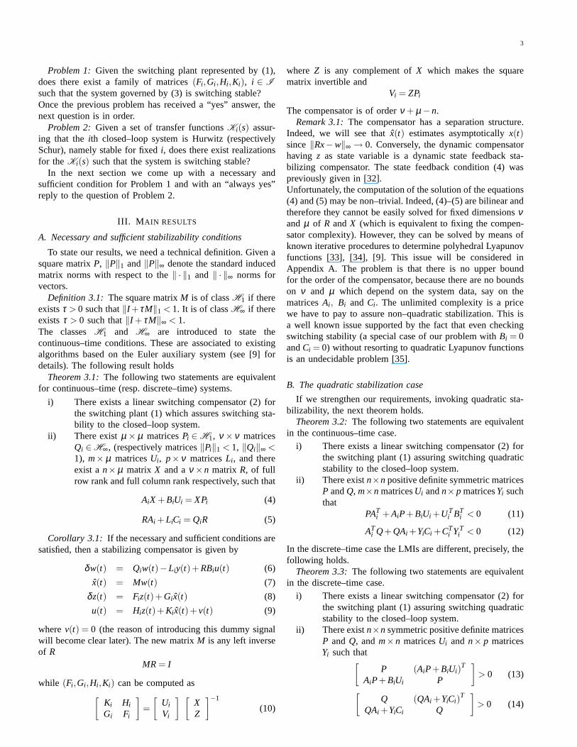
Problem 1: Given the switching plant represented by (1),does there exist a family of matrices(Fi ,Gi ,Hi ,Ki), i ∈ I

such that the system governed by (3) is switching stable?Once the previous problem has received a “yes” answer, thenext question is in order.

Problem 2: Given a set of transfer functionsKi(s) assur-ing that theith closed–loop system is Hurwitz (respectivelySchur), namely stable for fixedi, does there exist realizationsfor the Ki(s) such that the system is switching stable?

In the next section we come up with a necessary andsufficient condition for Problem 1 and with an “always yes”reply to the question of Problem 2.

III. M AIN RESULTS

A. Necessary and sufficient stabilizability conditions

To state our results, we need a technical definition. Given asquare matrixP, ‖P‖1 and‖P‖∞ denote the standard inducedmatrix norms with respect to the‖ · ‖1 and ‖ · ‖∞ norms forvectors.

Definition 3.1: The square matrixM is of classH1 if thereexistsτ > 0 such that‖I +τM‖1 < 1. It is of classH∞ if thereexistsτ > 0 such that‖I + τM‖∞ < 1.The classesH1 and H∞ are introduced to state thecontinuous–time conditions. These are associated to existingalgorithms based on the Euler auxiliary system (see [9] fordetails). The following result holds

Theorem 3.1:The following two statements are equivalentfor continuous–time (resp. discrete–time) systems.

i) There exists a linear switching compensator (2) forthe switching plant (1) which assures switching sta-bility to the closed–loop system.

ii) There existµ × µ matricesPi ∈ H1, ν ×ν matricesQi ∈ H∞, (respectively matrices‖Pi‖1 < 1, ‖Qi‖∞ <1), m× µ matricesUi , p× ν matricesLi , and thereexist an×µ matrix X and aν ×n matrix R, of fullrow rank and full column rank respectively, such that

AiX +BiUi = XPi (4)

RAi +LiCi = QiR (5)

Corollary 3.1: If the necessary and sufficient conditions aresatisfied, then a stabilizing compensator is given by

δw(t) = Qiw(t)−Liy(t)+RBiu(t) (6)

x(t) = Mw(t) (7)

δz(t) = Fiz(t)+Gi x(t) (8)

u(t) = Hiz(t)+Ki x(t)+v(t) (9)

wherev(t) = 0 (the reason of introducing this dummy signalwill become clear later). The new matrixM is any left inverseof R

MR= I

while (Fi ,Gi ,Hi ,Ki) can be computed as[

Ki Hi

Gi Fi

]

=

[Ui

Vi

] [XZ

]−1

(10)

where Z is any complement ofX which makes the squarematrix invertible and

Vi = ZPi

The compensator is of orderν + µ −n.Remark 3.1:The compensator has a separation structure.

Indeed, we will see that ˆx(t) estimates asymptoticallyx(t)since‖Rx−w‖∞ → 0. Conversely, the dynamic compensatorhaving z as state variable is a dynamic state feedback sta-bilizing compensator. The state feedback condition (4) waspreviously given in [32].Unfortunately, the computation of the solution of the equations(4) and (5) may be non–trivial. Indeed, (4)–(5) are bilinearandtherefore they cannot be easily solved for fixed dimensionsνandµ of R andX (which is equivalent to fixing the compen-sator complexity). However, they can be solved by means ofknown iterative procedures to determine polyhedral Lyapunovfunctions [33], [34], [9]. This issue will be considered inAppendix A. The problem is that there is no upper boundfor the order of the compensator, because there are no boundson ν and µ which depend on the system data, say on thematricesAi , Bi and Ci . The unlimited complexity is a pricewe have to pay to assure non–quadratic stabilization. This isa well known issue supported by the fact that even checkingswitching stability (a special case of our problem withBi = 0andCi = 0) without resorting to quadratic Lyapunov functionsis an undecidable problem [35].

B. The quadratic stabilization case

If we strengthen our requirements, invoking quadratic sta-bilizability, the next theorem holds.

Theorem 3.2:The following two statements are equivalentin the continuous–time case.

i) There exists a linear switching compensator (2) forthe switching plant (1) assuring switching quadraticstability to the closed–loop system.

ii) There existn×n positive definite symmetric matricesP andQ, m×n matricesUi andn× p matricesYi suchthat

PATi +AiP+BiUi +UT

i BTi < 0 (11)

ATi Q+QAi +YiCi +CT

i YTi < 0 (12)

In the discrete–time case the LMIs are different, precisely, thefollowing holds.

Theorem 3.3:The following two statements are equivalentin the discrete–time case.

i) There exists a linear switching compensator (2) forthe switching plant (1) assuring switching quadraticstability to the closed–loop system.

ii) There existn×n symmetric positive definite matricesP and Q, andm×n matricesUi and n× p matricesYi such that

[

P (AiP+BiUi)T

AiP+BiUi P

]

> 0 (13)

[

Q (QAi +YiCi)T

QAi +YiCi Q

]

> 0 (14)

4

Corollary 3.2: If the necessary and sufficient conditions aresatisfied, then a stabilizing compensator is given by

δ x(t) = (Ai +LiCi +BiJi)x(t)−Liy(t)+Biv(t)u(t) = Ji x(t)+v(t)

(15)

with v(t) = 0 (again this signal will be used later), and where

Ji = UiP−1 and Li = Q−1Yi

whereP andQ are the symmetric matrices defined in (11) and(12) (or by (13) and (14) in the discrete–time case).

Remark 3.2:This compensator has also an observer–basedstructure. It is of ordern, and thus of fixed complexity. Thisshows that, for switching systems, quadratic stabilizability isequivalent to quadratic stabilizability by means of a compen-sator of the same order of the plant.Note that (11)–(12) and (13)–(14) are LMIs, thus easilysolvable. We stress that this kind of conditions are knownin the LMI literature for both state feedback and observerdesign [12], [13], [36]. They have been proposed for instancefor LPV systems [12] (see also [10]). In [12] when the LMIsare stated (Th. 4.3) it is assumed thatB and C are certainmatrices. This is a critical assumption in the LPV case but notan issue in the switching case. The conditions based on LMIsand quadratic functions lead to efficient algorithms but they areconservative. Indeed, there are switching stable systems whichdo not admit quadratic Lyapunov functions. Less conservativeresults can be achieved if one considers synthesis results basedon parameter–dependent Lyapunov functions [14], [37], [38].

C. The set of all stabilizing compensators

In this section, we consider the problem of parametrizingall the switching compensators which can be associated withaswitching plant. An efficient parametrization setup is achievedby means of an observer–based pre-compensator and an inputinjection [5] (see also [6]). We adapt such a structure (whichcan be derived if the provided stabilizability conditions aresatisfied) to switching plants. Once the pre-compensator isdetermined, the free parameter is a proper stable transferfunction which must be properly realized, in agreement withthe results presented in [23] for the case of a single plant.

Henceforth, we will always assume stabilizability conditions(quadratic stabilizability) are satisfied. The main resultof thissubsection is simply stated as follows.

Theorem 3.4:Assume that the necessary and sufficient con-ditions for switching stabilizability of Theorem 3.1 (switchingquadratic stabilizability of Theorem 3.2 or Theorem 3.3)are satisfied. Then, given any arbitrary family of transferfunctions Ki(s), i = 1, . . . , r each stabilizing thei-th plant,there exists a switching compensator of the form (2) such thatHi(sI−Fi)

−1Gi + Ki = Ki(s) and such that the closed–loopsystem is switching stable (switching quadratically stable).The realization of such compensatorKi(s) is illustrated in Fig.2. More precisely, consider the observer–based compensator(6)-(9) or (15) and, instead of assumingv≡ 0, take

v(s) = Ti(s)(y(s)−y(s))

ui

i

i

i

u y

xi

i

ii

Ci

o

B C

F H

T

A

RBL M i

G K+

+

+

+−

+

ν

stab

Q

i

i iOBSERVER

PLANT

ESTIM. STATE FEEDBACK

Figure 2. The observer–based compensator structure

wherey(t) = Ci x(t) is the estimated output, namely

u(s) = ustab(s)+v(s) = ustab(s)+Ti(s)(Ci x(s)−y(s)) (16)

In other words,ustab is derived by means of the feedback(6)–(9) (or (15)), andTi(s) is a stable transfer function (theYoula–Kucera parameter [24], [25]). Note that the structure inFig. 2 is valid for both types of observer–based compensators(indeed, (6)–(7) parametrize all types of observers for fixed i[31], [30]) including (15) as special case withQi = Ai +LiCi ,R= I andM = I .

The transfer functionTi(s) can be selected in such a waythat the resulting compensator transfer function is the desiredoneKi(s)2. The only problem withTi(s) is its implementation,which cannot be arbitrary. In this case it is sufficient to exploitthe idea of [23] and realizeTi(s) as

Ti(s) = Hi(T)

(

sI−F(T)i

)−1G(T)

i +K(T)i

in such a way that the familyF (T)i is switching stable. This

results in switching stability and transfer function matchingfor any i. The procedure for control synthesis is the following

Procedure 3.1:Given Ki(s) i = 1, . . . , r each stabilizing(Ai ,Bi ,Ci) perform the following operations.

1) Check if the switching plant(Ai ,Bi ,Ci) satisfies thenecessary and sufficient conditions and, synthesize anystabilizing control of the form (6)–(9) (or (15)).

2) Select the free stable parameterTi(s) in such a way thatthe ith compensator has transfer functionKi(s). This isalways possible according to Lemma 10.2 in [5].

3) Select a Hurwitz (Schur) realization for eachTi(s). Makeall these realizations of the same order, possibly addingdummy non reachable and non–observable asymptoti-cally stable dynamics:

Ti(s) = H(T)i

(

sI− F(T)i

)−1G(T)

i + K(T)i

2in the case of a standard observer (15) this result is well established [5],but it will require some attention to deal with extended observers (6)–(9)

5

4) Find a realization (F (T)i ,G(T)

i ,H(T)i ,K(T)

i ) for Ti(s)which is switching–stable as follows. Take the previousrealizations(F (T)

i ,G(T)i ,H(T)

i , K(T)i ) and apply a transfor-

mation to each of them in such a way that all the statematricesF(T)

i share‖ · ‖22, the square of the Euclidean

norm, as a Lyapunov function. This can be done bysolving the Lyapunov equations

F (T)T

i Πi + ΠiF(T)i = −I

(positive definite solutionΠi exist sinceF (T)i is stable

by construction). In the discrete–time, use the analogousLyapunov equations. Denote byΩi the positive squareroot of Πi , say such thatΠi = Ω2

i . Apply the transfor-mation [23] (an alternative is to use proper reset maps)

F (T)i = ΩiF

(T)i Ω−1

i , G(T)i = ΩiG

(T)i ,

H(T)i = H(T)

i Ω−1i , K(T)

i = K(T)i

5) Realize the compensator as in Fig. 2.

The next corollary formalizes the fact that, if we are seekinga single compensator transfer function for all plants, ourparametrization works as well.

Corollary 3.3: Assume that the stabilizability conditionsare satisfied. Then a single compensatorC(s) stabilizes theplant (under switching) if and only if it can be representedas in Fig. 2 with a properTi (suitably realized). Moreover,if there existsC(s) such that all the closed–loop systems areHurwitz (Schur) stable, then there exist proper realizations forC(s) such that the overall system is switching stable.

Remark 3.3:Clearly, we have no guarantee that a singlerealization of a compensator which assures Hurwitz (Schur)stability preserves stability also under switching. This propertybecomes true under suitable and, in general, different realiza-tions of such a compensator.

IV. PROOFS OF THE RESULTS

To prove the results we need several preliminaries. The firstlemma is a key point.

Lemma 4.1:The following statements are equivalent forcontinuous–time (discrete–time) systems.

• The system

δx(t) = Aix(t), i = 1, . . . , r

is (switching) stable.• There exist a full row rank matrixX and r matricesPi ∈

H1 (‖Pi‖1 < 1 in the discrete–time case) such that

AiX = XPi

(equivalently, the norm‖x‖X,1.= min‖p‖1 : x = X p is

a polyhedral Lyapunov function)• There exist a full column rank matrixR and r matrices

Qi ∈H∞ (‖Qi‖∞ < 1, in the discrete–time case) such that

RAi = QiR

(equivalently, the norm‖x‖R,∞.= ‖Rx‖∞ is a polyhedral

Lyapunov function).

Proof: The Lemma is nothing else that a re–statement ofwell–known results due to [27], [28] and to [29], [26]. Indeed,the stability of the switching system is equivalent to the robuststability of the corresponding LPV system (see [27], Th. 5 or[26] Part I, Th. 1)

δx(t) =

[r

∑i=1

Aiwi(t)

]

x(t),r

∑i=1

wi(t) = 1, wi(t) ≥ 0.

Precisely, the first equation is eq. (8) in [29] Part III, Thesecond equation is its dual. As far as the discrete–timeequations are concerned, the first is given in [26] (see PartII, Theorem 1), the second (the dual) can be derived by thedual systemδx = AT

i x which is switching stable if and onlyif δx = Aix is such ([26], Part I, Th. 3). Duality between thetwo equations has been also investigated in [15].

Remark 4.1:As a special case of the lemma withX = I orR= I , a switching system governed by the matricesPi ∈H1 orQi ∈ H∞ (resp.‖Pi‖1 < 1 or ‖Qi‖∞ < 1, in the discrete–timecase) is stable, because it admits‖ ·‖1 or ‖ ·‖∞ as a Lyapunovfunction. Note that in general we know thatX has at least asmany columns as rows and thatR has at least as many rowsas columns, but no upper bound can be established.

A. Proof of Theorem 3.1 and Corollary 3.1

Proof: i) ⇒ ii) (or iii) for discrete time systems).Assume that (1) is stabilized by (2). Then, in view of Lemma4.1, the following set of equations

Acli X =

[Ai +BiKiCi BiHi

GiCi Fi

] [X1

X2

]

=

[X1

X2

]

Pi (17)

hold for i = 1, . . . , r, with Pi ∈ H1 (or ‖Pi‖1 < 1, in thediscrete–time case). Here the full row rank matrixX has beenpartitioned according to the partition ofAcl

i . If we take theupper–left block we have

AiX1 +BiKiCiX1 +BiHiX2 = AiX1 +BiUi = X1Pi

with Ui = KiCiX1 + HiX2. SinceX is full row rank, so isX1.This proves equation (4). The dual equation (5) can be provedexactly in the same way starting from

[R1 R2] Acli = Qi [R1 R2] (18)

with Qi ∈ H∞ (‖Qi‖∞ < 1, in the discrete–time case).ii) (or iii) for discrete time systems) ⇒ i). To prove the

sufficiency, the first step is to show that, if (5) holds, thenthe first two equations (6)–(7) of the proposed compensatorrepresent an extended observer [31], [30] for the system3.Multiply the plant state equation byR and subtract (6)

δ (Rx(t)−w(t)) =

= RAix(t)+RBiu(t)−Qiw(t)+Liy(t)−RBiu(t)

= RAix(t)−Qiw(t)+LiCix(t) = Qi(Rx(t)−w(t))

3this was shown in [15] in the LPV context, withB andC constant matrices,and it is reported here for completeness

6

Since Qi ∈ H∞ (or ‖Qi‖∞ < 1) the corresponding system isstable (see Remark 4.1) and therefore‖Rx(t)−w(t)‖→ 0 and,in view of (7),

M[Rx(t)−w(t)] = x(t)− x(t) → 0

As a second step, we show that if (4) holds, then the equations(8)–(9) represent a stabilizing state feedback compensator(if we replace ˆx(t) by x(t)). Indeed, the closed–loop matrixsatisfies the equation

[Ai +BiKi BiHi

Gi Fi

] [XZ

]

=

[XZ

]

Pi

as it can be immediately verified from (10). Since, by con-struction,[XT ZT ]T is invertible, in view of Lemma 4.1, thestate feedback is stabilizing.

To prove closed–loop switching stability, consider the newvariable

e(t) = w(t)−Rx(t), so that ˆx(t)−x(t) = Me(t) (19)

Assuming x(t), z(t) and e(t) as state variables, we get thefollowing overall closed–loop matrix

Ai +BiKi BiHi BiKiMGi Fi GiM0 0 Qi

(20)

The corresponding block–triangular switching system is stableif and only if its diagonal blocks are switching stable ([29],Part I). The first diagonal block (which comes from the “statefeedback”) has been just proved to be switching stable. The“error system” governed byQi is also stable (see Remark 4.1)so the proof is completed.

B. Proof of Theorem 3.2

We give a formal proof of Theorem 3.2 in the continuous–time case only. The proof of Theorem 3.3, the discrete–timeversion, is similar.

Proof: i) ⇒ ii) If (1) is quadratically stabilized by (2),then by definition there exists a symmetric positive definitematrix P such that

(Acl

i

)P + P

(Acl

i

)T< 0. After a proper

partition, we write[

Ai +BiKiCi BiHi

GiCi Fi

] [P11 P12

PT12 P22

]

+[

P11 P12

PT12 P22

][Ai +BiKiCi BiHi

GiCi Fi

]T

< 0

If we take the left upper block of the previous expression,denoting byUi

.= KiCiP11+HiPT

12, we have

(Ai +BiKiCi)P11+(BiHi)PT12+P11(Ai +BiKiCi)

T+P12(BiHi)

T = AiP11+P11ATi +BiUi +UT

i Bi < 0

which is eq. (11). The dual equation (12) is derived exactlyin the same way.

ii) ⇒ i). Assume that (11) and (12) hold and take the lineargainsJi =UiP−1 andLi = Q−1Yi . Consider now the observer–based feedback compensator (15) and consider the variables

x1(t) = x(t) andx2(t) = x(t)−x(t) to achieve the closed–loopsystem matrix

[Ai +BiJi BiJi

0 Ai +LiCi

]

Both diagonal blocks are quadratically stable with Lyapunovmatrices given byP andQ, respectively, since

P(Ai +BiJi)T +(Ai +BiJi)P = PAT

i +UTi BT

i +AiP+BiUi < 0(Ai +LiCi)

TQ+Q(Ai +LiCi) = ATi Q+CT

i YTi +QAi +YiCi < 0

It is then trivial to prove that this system is quadraticallystablesince, by the previous inequalities,

[P 00 θQ−1

][Ai +BiJi BiJi

0 Ai +LiCi

]T

+[

Ai +BiJi BiJi

0 Ai +LiCi

][P 00 θQ−1

]

< 0

provided thatθ > 0 is large enough.

C. Proof of Theorem 3.4

The proof of this result is quite technical in the generalcase and much simpler in the quadratic stability frameworksince it involves tools which are available on most (ad-vanced) books. Therefore, we first consider the quadratic case.Let us first recall the following fundamental lemma, whichgives an observer based interpretation of the Youla–Kuceraparametrization of all stabilizing compensators.

Lemma 4.2:[5] Given a stabilizable plant(A,B,C), the setof all stabilizing linear compensators is given by

δ x(t) = (A+LC+BJ)x(t)−Ly(t)+Bv(t)u(t) = Jx(t)+v(t)o(t) = C(x(t)−x(t))v(s) = T(s)o(s)

(21)

whereA+BJ and A+LC are Hurwitz (Schur) andT(s) is asuitable stable transfer function.

Proof: (Theorem 3.4, the quadratic stability case).The proof of Theorem 3.4 under the quadratic stabilizabilityconditions of Theorem 3.2 is easy. Indeed the structure of thecompensator (15) is exactly that prescribed in Lemma 4.2.Therefore there exists a properTi(s) such that thei-th transferfunction is anyKi(s) which makes thei-th plant Hurwitz. Theonly remaining point is the determination of proper switchingstable realizations for the familyTi(s). In view of [23], suchrealizations can be determined according to Procedure 3.1,Step 4. Intuitively, if we take such a realization, then “Ti(s)sees no feedback” sinceo(t) → 0 no matter whatv(t) does,therefore the overall system remains switching stable. We willcome back on this issue later to provide a formal proof.

The next lemma shows how the parametrization of [5],based on a Luenberger observer, can be extended if we adopta generalized observer, as defined in [31], [30].

Lemma 4.3:Given a stabilizable plant(A,B,C), assumethat there exist a Hurwitz (Schur) matrixQ, a matrix L, afull column rank matrixR, a full row rank matrixM such that

RA+LC = QR, MR= I (22)

7

and matricesF, G, H, K such that

u(s) =[H(sI−F)−1G+K

]x(s)

is a stabilizing state feedback compensator. Then

δw(t) = Qw(t)−Ly(t)+RBu(t) (23)

x(t) = Mw(t) (24)

δz(t) = Fz(t)+Gx(t) (25)

u(t) = Hz(t)+Kx(t)+v(t) (26)

o(t) = C(x(t)−x(t)) (27)

v(s) = T(s)o(s) (28)

parametrize all the stabilizing compensators for(A,B,C).Proof: The fact that any compensator of the form (23)–

(28) is stabilizing is not proved here, since it will be provedin the more general (switching) case later. Thus we prove nowthat any givenK (s) which stabilizes(A,B,C) can be writtenas in (23)–(28).

Augment equation (22) as follows

[R S

][

A Φ0 Aη

]

+L[

C 0]= Q

[R S

](29)

whereS is a complement ofR (i.e. [R S] is invertible) and[

ΦAη

]

=[

R S]−1

QS

We need the following:Claim 4.1: Matrix S can be taken in such a way thatAη is

Hurwitz (Schur). The proof is given in Appendix B.Therefore, assume thatAη is stable. Consider the followingtransformation4

w =[

R S]

[ϕη

]

or

[ϕη

]

=[

R S]−1

w

for (23) and (24) so as to achieve[

δ ϕδ η

]

=[

R S]−1

Q[

R S][

ϕη

]

−[

R S]−1

Ly+[

R S]−1

RBu

namely[

δ ϕδ η

]

=

[A+ L1C Φ

L2C Aη

][ϕη

]

−

[L1

L2

]

y+

[B0

]

u (30)

x = ϕ +MSη (31)

where [L1

L2

]

=[

R S]−1

L

Now we apply the transformation to (25) and (26) to achieve(we use the dummy substitutionζ = z)

δ ζ = F ζ +Gϕ +GMSη (32)

u = Hζ +Kϕ +KMSη +v (33)

4we are putting “hats” on these variables because they will beshown to beestimators

The equations (30)–(33) represent an observer–based stabiliz-ing compensator for the fictitiously extended plant

δϕδηδζ

=

A Φ 00 Aη 00 0 Aζ

︸ ︷︷ ︸

Aaug

ϕηζ

+

B 00 00 I

︸ ︷︷ ︸

Baug

[uσ

]

(34)

y =[

C 0 0]

︸ ︷︷ ︸

Caug

ϕηζ

(35)

where Aζ is an arbitrary stable matrix andσ a fictitiousinput. Let us now observe that theη and ζ dynamics are,respectively, unreachable and unobservable. Note also that inno way σ can stabilize/destabilize the system. It is apparentthat K (s) stabilizes the original plant if and only if

[K (s)

0

]

(36)

stabilizes (34)–(35). Since, by construction, (34)–(35) is sta-bilizable (the original(A,B,C) system is such, and the addedunreachable/unobservable dynamics are asymptotically stable),the set of all stabilizing compensators, according to Lemma4.2 applied to the extended plant, is given by

δ ϕδ ηδ ζ

=

A Φ 00 Aη 00 0 Aζ

ϕηζ

+

B 00 00 I

[K KMS HG GMS F−Aζ

]

︸ ︷︷ ︸

Jaug

ϕηζ

+

L1

L2

0

︸ ︷︷ ︸

Laug

[C 0 0]

ϕηζ

−

L1

L2

0

y+

B 00 00 I

[vρ

]

(37)

[uσ

]

=

[K KMS HG GMS F−Aζ

]

ϕηζ

+

[vρ

]

(38)

[vρ

]

=

[T(s)T(s)

]

o(s) =

[T(s)T(s)

]

[y−y] (39)

therefore the compensator (36) can be written in this form.The proof is now concluded if one notices that (37)–(39) isexactly of the form (30)–(33) (if one disregards the fictitiousinput σ ).

We are now in the position of proving Theorem 3.4.Proof: (Theorem 3.4, switching stability)Consider the

compensator equations (6)–(9) with the input injection (16).Denote byz(T) the state of any switching stable realization forthe (stable) transfer functionsTi(s)

δz(T)(t) = F (T)i z(T)(t)+G(T)

i o(t), (40)

v(t) = H(T)i z(T)(t)+K(T)

i o(t) (41)

and consider the state variablesx(t), z(T), z(t), and e(t) =w(t)− Rx(t). Without restriction, we assume thatall theserealizations have the same dimension, a condition which can

8

be possibly met by adding stable redundant dynamics. Then,bearing in mind thatMR= I , that from (19) ˆx−x = Me andthat from (27)o = CMe, we have that

δx = Aix+Biu = Aix+BiKi x+BiHiz+Biv =

= Aix+BiKix+BiKiMe+BiHiz+Bi(K(T)i o+H(T)

i z(T))

= (Ai +BiKi)x+Bi(Ki +K(T)i Ci)Me+BiHiz+BiH

(T)i z(T)

and thatδz= Fiz+Gi x = Fiz+Gix+GiMe

Since δe = Qie, we can cast the closed–loop system in theform δxcl = Acl

i xcl with xcl = [xT zT z(T)TeT ]T and

Acli =

Ai +BiKi BiHi BiH(T)i Bi(Ki +K(T)

i Ci)MGi Fi 0 GiM

0 0 F (T)i G(T)

i CiM0 0 0 Qi

This matrix is in an upper block–triangular form and then thesystem is stable if and only if the diagonal blocks are such([26], Part 1, Th. 1). The stability of the first block has beenproved in Subsection IV-A (see eq. (17)). The second block isstable because we took a switching stable realization for theYoula–Kucera parameters (F(T)

i is switching stable) and thesubsystem governed byQi is switching stable (see Remark4.1). Thus the proposed construction produces a switchingstabilizing compensator for any switching stable realization(40) (41) ofTi(s).

The proof is now over in view of Lemma 4.3. Indeedfor fixed i ∈ I , equations (23)–(28) represent any stabilizingcompensator for thei-th plant, with proper functionsTi(s).

We conclude the section pointing out that, since we even-tually come up with a Lyapunov function, a generalization ofAssumption 1 is possible, because as long as we can definegeneralized solution we could show that the correspondingLyapunov derivative is negative almost everywhere.

V. I MPLICATIONS OF THE RESULTS

A. Switching systems and optimization

Consider the problem of optimizing a set of plants

δx(t) = Aix(t) +Biu(t) +Bωi ω(t)

y(t) = Cix(t) +Dy,ωi ω(t)

ξ (t) = Eix(t) +Dξ ,ui u(t) +Dξ ,ω

i ω(t)(42)

according to some criteria. Hereω(t) and ξ (t) representany disturbance–input and performance–output relevant tothe problem. Assume that a family of compensatorsKi(s)(optimal for fixed i) is designed. Then, in view of Theorem3.4, we can combine them together according to the followingproposition.

Proposition 5.1: If the switching system satisfies the nec-essary and sufficient conditions, then there exists a switchingcompensator(Fi,Gi ,Hi ,Ki) which

• achieves optimality for any fixed configurationi;• assures stability under switching.

Once we have computed the observer–based pre–compensator(see Fig. 3) thei-th input output map is of the form

ξ (s) = [Mξ ,ωi (s)+Mξ ,v

i (s)Ti(s)Mo,ωi (s)]ω(s)

whereMξ ,ωi (s), Mξ ,v

i (s) andMo,ωi (s) are theω–to–ξ , v–to–ξ

andω–to–o transfer functions for thei-th configuration. This

u

iT

x

Ci

o

PLANT

FEEDBACKSTATE

OBSERVER

SWITCHING

SWITCHING

ω ξ

u y

estimatedstate

+

ν+

+

−

stab

Figure 3. The optimization setup

is an important feature, since it allows for the well–knownWiener-Hopf design [25] for theith transfer function (whichis affine with respect toTi ). Stability is eventually assured bythe realization (40)–(41).

As a final remark we stress an essential difference from theprevious (inspiring) work [23]. Roughly, Hespanha and Morseidea is to show that, for a single plant you may constructasinglepre–compensator and freely “switch among the Youla–Kucera parametersTi(s)”. In brief a singleM instead ofMi issufficient for a single plant. Here we extend the idea, but wecannot rely, in general, on a single pre–compensator.

B. Contractive design

In practice, stability may be a goal which is not sufficientand one might require the overall switching system to satisfycertain performance requirements in terms of convergencespeed. For a single plant this boils down to assigning thepoles. The natural question is whether we can enforce aconvergence speedeven under switching. We consider forbrevity the discrete–time case only. Assume that we wish toassure a speed of convergenceλ , 0≤ λ < 1 to the system,namely

‖x(t)‖ ≤ γ‖x(0)‖ λ t

Then we can work with the modified system

δx(t) = Aiλ x(t)+Biu(t)

y(t) = Cix(t)(43)

For this switching system to admit a solution, the necessaryand sufficient conditions (4) and (5) must hold

AiX +Bi(λUi) = X(λPi) (44)

9

RAi +(λLi)Ci = (λQi)R (45)

If the above are satisfied, it is possible to setλUi = Ui , λLi = Li

and, most importantly,

Pi = λPi , and Qi = λQi

It is immediate to see that, since‖Qi‖∞ < 1 and‖Pi‖1 < 1, then‖Qi‖∞ < λ and‖Pi‖1 < λ . These new matrices are responsiblefor the convergence speed of the overall switching system(even under switching) and this assures a speed of convergenceλ with the pre–compensator (6)–(9). It is not difficult to seethat, given any choice ofTi(z) with all the poles in the openλ–disk, it is possible to find proper realizations which areλ–switching stable5 and thus the overall realization of thecompensator+Youla–Kucera parameter assures a globalλ–convergence. Working with the modified system is basicallyequivalent to fixλ in the procedure to determine the polyhedralfunction, reported in Appendix A.

C. The zero transfer functions paradox

Assume that we are given a plant composed by a (finite)family of switching systems which are Hurwitz (Schur), butnot switching stable. According to Theorem 3.4, if this plantis switching stabilizable, then we can apply a switchingcompensator such that the system is switching stable, but,at the same time, for any fixedi the compensator transferfunction isKi(s) ≡ 0. A potential application of this propertyis what we call the switching manager (Fig. 4), a device whichleaves the plant uncontrolled as long as it remains on a fixedconfiguration (for instance because optimal compensators arealready applied for eachi) and produces a control action onlyunder switching.

u yi

SWITCHING

MANAGER

(for fixed i)

OPTIMAL PLANTS

Figure 4. The switching manager: a switching stabilizing control having 0transfer function for eachi

Let (Ai ,Bi ,Ci) be a continuous–time switching plant. Forthe simple exposition, let us assume quadratic stabilizability(the property holds also in the general case). LetJi and Li

be the linear gains obtained as in Corollary 3.2. A switchingstabilizing observer–based compensator is the following:

˙x = Ai x+Li(Ci x−y)+Biuu = Ji x+vz = ΩiAiΩ−1

i z+ ΩiLi(Ci x−y)v = −JiΩ−1

i z

(46)

5i.e. the associated switching system assures a convergencespeedλ

whereΩi is the transformation previously introduced (chosenin such a way thatΩiAiΩ−1

i is switching stable and admitszTz as a common Lyapunov function). Let us write it as[

˙xz

]

=

[Ai +BiJi +LiCi −BiJiΩ−1

iΩiLiCi ΩiAiΩ−1

i

][xz

]

+

[−Li

−ΩiLi

]

y

u =[

Ji −JiΩ−1i

][

xz

]

It is immediate to see that (for any choice ofΩi) the transferfunction from y to u is zero. Indeed, consider the followingchange of variables

[q1

q2

]

=

[x

x−Ω−1i z

]

,

[xz

]

=

[q1

Ωi (q1−q2)

]

to get[

q1

q2

]

=

[Ai +LiCi BiJi

0 Ai +BiJi

][q1

q2

]

+

[−Li

0

]

y

u =[

0 Ji][

q1

q2

]

This compensator has 0–transfer function, for fixedi, as it canbe verified by direct calculation (the system Markov parame-ters are all 0). However, to better explain the phenomenon, welet the reader notice that the two componentsq1 andq2 of thevectorq are unobservable and unreachable respectively. Froma geometric point of view, the reachable subspace is includedin the q1–subspace and thus in the unobservable subspace.Since the transformation depends oni, this property is clearlytrue for fixedi only and we will see the consequences soon.

To check the overall stability consider the state vectorcomposed byx, e = x− x and z. The resulting equationsbecome

xez

=

Ai +BiJi BiJi −BiJiΩ−1i

0 Ai +LiCi 00 ΩiLiCi ΩiAiΩ−1

i

xez

y =[

Ci 0 0]

xez

Given its upper block–triangular structure, the state matrix isswitching stable.

As a simple example, consider the system with two vertices

x =

[0 1

−2+ γ −0.01

]

x+

[01

]

u

y =[

1 0]x

(47)

whereγ ∈ −1, 1. Denote byA1 and A2 the values of thestate matrix forγ = −1 and 1, respectively. Although eachAi

is Hurwitz, the time-varying system governed by the switchrule γ(t) = sign[x1(t)x2(t)] (xi represents the state component)is unstable (see [8] for details). The phase portrait of the freeevolution with the adopted switching rule andx(0) = [0 1]T

is reported in Fig. 5 (top). By means of the next observer andstate feedback gains

L1 = L2 =

[−10

0

]

, J1 = J2 =[

0 −10]

10

switching stability is assured. A switching regulator can berealized in such a way that its transfer function is zero foreachi which is given by (46) with

Ω1 =

[14.142 0.00750.0075 8.165

]

, and Ω2 =

[10.001 0.02450.025 10.00

]

The state–space evolution of the closed–loop system is re-ported in Fig. 5 (bottom). Finally, the control input evolution

−8 −6 −4 −2 0 2 4 6 8

−4

−2

0

2

4

6

8

x1

x 2

−1 −0.5 0 0.5 1 1.5

−1

−0.5

0

0.5

1

x1

x 2

Figure 5. The unstable state–space evolution of system (47)with switchingrule γ(t) = sign[x1(t)x2(t)] (top) and the corresponding evolution with theswitching manager (bottom)

(which becomes active only under switching) is reported inFig. 6.

0 50 100 150 200 250 300 350 400−3

−2

−1

0

1

2

3

4

5

t

u

Figure 6. The input evolution of system (47) in closed–loop

Although the fact that switching stability for stabilizableHurwitz plants can be achieved with a compensator such thatKi(s) ≡ 0, is a consequence of Theorem 3.4, we would liketo give a simple explanation for this paradox. The proposedtechnique produces a compensator realization which is non–minimal. In fact, for fixed i, the realization reachable and

observable subspaces have trivial intersection. The situationis different under switching since the actual “reachable” and“observable” subspace are “larger” than those of the singlerealizations (see [39], Section 4, for details). The “separation”between the reachable and observable subsystems is not trueanymore and the interaction (possible under switching) impliesthat the input–output map is non–zero. This allows for astabilizing feedback action.

VI. EXAMPLE

We present a very simple (academic) example to show thatinstability problems due to switching can arise in very simplecases. Consider the system in Figure 7 where a fluid flowsthrough two–tanks. The state values are the reservoir levels

sensor 2sensor 1

actuator 1 actuator 2

Figure 7. The two–tank system

(with respect to their nominal values—the dashed lines). Theflow between the two reservoirs is proportional to the differ-ence of their levels. We assume that both flow control and levelmeasurement can switch arbitrarily from the form the first tank(actuator 1 –sensor 1) to the second tank (actuator 2 –sensor2). We assume that, if uncontrolled, the incoming and outgoingflows are constant and equal to the nominal values. For thissystem the state matrix remains clearly unchanged while theinput and output matrices can switch. We derive the next modelwith two vertices (including input and measurements noises)

x(t) =

[−1 1

1 −1

]

x(t)+Biu(t)+wx(t)

y(t) = Cix(t)+wy(t)

where the ones inA are achieved by time–normalization andwhere the input and output (normalized) matrices are

B1 =

[10

]

, B2 =

[0−1

]

C1 =[

0 1], C2 =

[1 0

]

We computed the optimal LQ and Kalman gainsJ(opt)i and

L(opt)i minimizing, respectively the cost

∫ ∞

0

(

1000x21(t)+10000x2

2(t)+1

10000u2(t)

)

dt

and the estimated state error covariance when the processnoise wx and output noisewy (Gaussian white noises withzero mean) have covariance matrices

Qwx =

[1/10 0

0 1/10

]

Qwy =1

1000

11

To enforce a certain convergence rate to the overall LQGcontroller, we shifted to the right the poles of the originalsystem by a valueα = 2 (say, we solved the LQ and Kalmanequations when the state matrix isA+ 2I ). The resultingoptimal compensatorsKi(s) are

q =(

A+BiJ(opt)i +L(opt)

i Ci

)

q−L(opt)i y

u = J(opt)i q

, i = 1,2

withJ(opt)

1 =[−3167.59 −13655.68

]

J(opt)2 =

[20491.14 10003.05

]

and

L(opt)1 =

[−27.64−13.50

]

L(opt)2 =

[−13.50−27.64

]

Unfortunately we have the followingClaim 6.1: If the controller are implemented directly, we

achieve the following closed–loop matrices

Acl1 =

−3168.59 −13682.32 0 27.64361 −14.5014 0 13.5014

−3167.59 −13655.69 −1 10 0 1 −1

Acl2 =

−14.5015 1 13.5015 0−20517.78 −10004.04 27.6436 0

0 0 −1 1−20491.14 −10003.05 1 −1

and the resulting system is switching unstable.The reader can easily verify the claim by computingthe exponential matrices and checking that the productexp[Acl

1 T]exp[Acl2 T] for T = 0.1 is not Schur. Therefore, the

continuous–time system diverges if we activate the two sys-tems alternatively in sampling periods of lengthT = 0.1.

However, the above switching system passes the switchingstabilizability test (even quadratic)6 and then we can computeany compensator for each subsystem and then realize itaccording to the proposed results. We computed the stabilizingswitching controllers guaranteeing a convergence rateα = 2.As a first step, we solved the two equations (4) and (5) forthe shifted systems and we derived the stabilizing controllers

Kstab

1 :

wuo

=

−2 14.4 0 −1−10 −24 20 5

60 −14.4 0 112

35 −1 0

wyv

Kstab

2 :

wuo

=

−2 −14.4 0 −110 −24 20 − 5

60 14.4 0 1− 1

235 −1 0

wyv

As a second step, we computed the Youla–Kucera parametersTi(s) (and we derived a switching stable realization of the two)in such a way that the lower linear fractional transformation[5] of the switching stabilizing controllers andTi(s), depictedin Fig. 8, results in the desired controllersKi(s). The state–

6we used the efficient code by M. Grant and S. Boyd. CVX: Matlabsoftware for disciplined convex programming [web page and software].http://www.stanford.edu/ boyd/cvx, October 2007

K11

stabK

12

stab

K21

stabK

22

stab

T(s)i

u(t)

o(t)v(t)

y(t)

Figure 8. Linear fractional transformation

space realizations of the (switching stabilizing) regulatorsK1

andK2 are reported Table I. Fig. 9 depicts the time evolutionof the system state and the switching signal.

0 0.5 1 1.5 2 2.5 3 3.5 4 4.5 5−3

−2.5

−2

−1.5

−1

−0.5

0

0.5

1

1.5

2

t

x2(t)

x1(t)

Figure 9. The state components and switching signal (top) evolutions

VII. D ISCUSSION AND CONCLUSIONS

In this paper, we have given necessary and sufficient sta-bilizability conditions for the existence of a stabilizingandquadratically stabilizing switching linear compensatorsfor aswitching plant. We have seen that if these conditions aresatisfied, no matter how we associate a family of compensatorswith a family of plants, then there exist realizations for whichthe closed–loop system is switching stable. We have shownhow to derive these realizations. In this way we extended theresults in [23], where switching compensators are applied toa single linear plant. The results have several implicationssuch as the “paradox of the zero transfer functions”, withits application to the switching manager, the optimal Wiener–Hopf synthesis and the contractive design. The general stabi-lizability conditions suffer of the well known problem of thecomplexity of the required algorithms and of the complexityof the compensator. Conversely, if we resort to the quadraticstabilizability, efficient LMI algorithms are involved andthecompensator has a complexity which is fixed a–priori.

The results are suitable for several extensions and we believethat there are several interesting issues to be investigated.

In the formulation of the problem we assumed that switch-ing is uncontrolled and that the compensator switches ac-cordingly, with full information and no delay. It would be

12

K1 :

[qu

]

=

−2 14.4 40355 9368.1 385.55 −10.812 0−10 −24 −33629 −7806.8 −321.29 9 20

−3.825 −4.59 −3000.1 −700.17 −28.78 0.77 7.651.9684 2.3621 −700.61 −169.96 −5.7987 0.094382 −3.93690.23811 0.28573 −31.484 −9.823 −2.9053 0.13585 −0.47621−0.01011 −0.012132 1.0243 0.2528 0.14111 −12.101 0.02022

0 −14.399 −40355 −9368.1 −385.55 10.812 0

[qy

]

K2 :

[qu

]

=

−2 −14.4 −32338 100043 433.14 −21.812 010 −24 −26948 83370 360.95 −18.176 20

3.4642 −4.157 −947.27 2922.4 13.162 −0.68434 6.9283−1.6446 1.9735 2922.5 −9058.6 −38.815 1.8882 −3.28920.24837 −0.29804 12.43 −41.824 −2.6076 0.25012 0.49673

−0.0099683 0.011962 −0.73804 2.2786 0.25167 −12.096 −0.0199370 14.4 32338 −100043 −433.14 21.812 0

[qy

]

Table ITHE STABILIZING COMPENSATOR REALIZATIONS

interesting to investigate the case of delayed informationorthe case in which the controller has to identify the currentsystem configuration. For the latter problem the observer–based structure of the proposed compensator seems to bepromising [40], [36]. In this work we have not consideredthe case in which the plant is switched, namely the discretevariable is a control signal (see for instance [39]). However,we believe that the presented results could be successfullyapplied to the switched case in the sense that the scheme canbe used to enforce stability jointly with another scheme whichcontrols switching to optimize performances. Another issuenot currently investigated is whether the current results canbe extended to LPV systems rather than switching systems.We conjecture that as long asB and C are constant andknown matrices, results along these line can be established.Finally we would like to point out that we have seen howto optimize the performances in each configuration whileassuring switching stability. The overall optimality problemis a non–trivial problem left to future investigation. The ideasproposed in the recent work [41] seem to be promising in thissense.

REFERENCES

[1] P. Antsaklis and A. Nerode, “Special issue on hybrid control systems,”IEEE Trans. Automat. Control, vol. 43, no. 4, 1988.

[2] R. A. Decarlo, M. S. Branicky, S. Pettersson, and B. Lennartson,“Perspectives and results on the stability and stabilizability of hybridsystems,”Proceedings of the IEEE, vol. 88, no. 7, pp. 1069–1082, 2000.

[3] D. Liberzon and A. S. Morse, “Basic problems in stabilityand designof switched systems,”IEEE Contr. Syst. Mag., vol. 19, no. 5, pp. 59–70,1999.

[4] T. I. Seidman, “Switching systems, i: general theory,” MD:UMBC, Baltimore, Tech. Rep., 1986. [Online]. Available:citeseer.ist.psu.edu/19046.html

[5] K. Zhou, J. Doyle, and K. Glower,Robust and Optimal Control.Englewood Cliff, NJ: Prentice-Hall, 1996.

[6] R. Sanchez-Pena and M. Sznaier,Robust systems, Theory and Applica-tions. New York: Wiley, 1998.

[7] M. S. Branicky, “Multiple Lyapunov functions and other analysis toolsfor switched and hybrid systems,”IEEE Trans. Automat. Control,vol. 43, no. 4, pp. 475–482, 1998.

[8] D. Liberzon,Switching in System and Control, ser. Systems and Control:Foundations & Applications. Boston: Birkhauser, 2003.

[9] F. Blanchini and S. Miani,Set–theoretic method in control, ser. Systemsand Control: Foundations and Applications. Boston: Birkhauser, 2003.

[10] S. Boyd, L. El Ghaoui, E. Feron, and V. Balakrishnan,Linear MatrixInequalities in System and Control Theory. SIAM, 2004.

[11] J. S. Shamma, “Linearization and gain scheduling,” inThe ControlHandbook, W. Levine, Ed. CRC Press, 1996, pp. 388–396.

[12] G. Becker and A. Packard, “Robust performance of linearparametri-cally varying systems using parametrically-dependent linear feedback,”Systems & Control Letters, vol. 23, pp. 205–215, 1994.

[13] P. Apkarian and P. Gahinet, “A convex characterizationof gain–scheduledH∞ controllers,”IEEE Trans. Automat. Control, vol. 40, no. 5,1995.

[14] E. Feron, P. Apkarian, and P. Gahinet, “Analysis and synthesis of robustcontrol systems via parameter-dependent Lyapunov functions,” IEEETrans. Automat. Control, vol. 41, no. 7, pp. 1041–1046, 1996.

[15] F. Blanchini and S. Miani, “Stabilization of LPV systems: state feedback,state estimation and duality,”SIAM J. Control Optim., vol. 42, no. 1,pp. 76–97, 2003.

[16] B. Barmish and M. Fu, “Adaptive stabilization of linearsystems viaswitching control,” IEEE Trans. Automat. Control, vol. 31, no. 12, pp.1097–1103, 1986.

[17] M. Chang and E. J. Davison, “Adaptive switching controlof lti mimosystems using a family of controllers approach,”Automatica J. IFAC,vol. 35, no. 3, pp. 453–465, 1999.

[18] J. Hespanha, D. Liberzon, and A. S. Morse, “Overcoming the limitationsof adaptive control by means of logic-based switching,”Systems &Control Letters, vol. 49, no. 1, pp. 49–65, 2003.

[19] A. S. Morse, “Supervisory control of families of linearset-point con-trollers. I: Exact matching,”IEEE Trans. Automat. Control, vol. 41,no. 10, pp. 1413–1431, 1996.

[20] ——, “Supervisory control of families of linear set-point controllers. II:Robustness,”IEEE Trans. Automat. Control, vol. 42, no. 11, pp. 1500–1515, 1997.

[21] O. Beker, C. V. Hollot, and Y. Chait, “Plant with integrator: an exampleof reset control overcoming limitations of linear feedback,” IEEE Trans.Automat. Control, vol. 46, no. 11, pp. 1797–1799, 2001.

[22] A. V. Savkin, E. Skafidas, and R. Evans, “Robust output feedbackstabilizability via controller switching,”Automatica J. IFAC, vol. 35,no. 1, pp. 69–74, 1999.

[23] J. Hespanha and A. S. Morse, “Switching between stabilizing con-trollers,” Automatica J. IFAC, vol. 38, no. 11, pp. 1905–1917, 2002.

[24] V. Kucera, Analysis and design of discrete linear control systems.Englewood Cliffs, NJ: Prentice Hall International, 1991.

[25] D. Youla, H. Jabr, and J. Bongiorno, J., “Modern Wiener-Hopf designof optimal controllers, ii. the multivariable case,”IEEE Trans. Automat.Control, vol. 21, no. 3, pp. 319–338, 1976.

[26] N. E. Barabanov, “Lyapunov indicator of discrete inclusion. part I-II-III,” Automat. Remote Control, vol. 49, pp. I: 152–157, II: 283–287, III:558–566, 1988.

[27] R. K. Brayton and C. H. Tong, “Stability of dynamical systems: aconstructive approach,”IEEE Trans. Circuits and Systems, vol. 26, no. 4,pp. 224–234, April 1979.

[28] ——, “Constructive stability and asymptotic stabilityof dynamical

13

systems,”IEEE Trans. Circuits and Systems, vol. 27, no. 11, pp. 1121–1130, November 1980.

[29] A. P. Molchanov and E. S. Pyatnitskii, “Lyapunov functions that definenecessary and sufficient conditions for absolute stabilityof nonlin-ear nonstationary control systems. I-II-III,”Automat. Remote Control,vol. 47, pp. I:344–354, II: 443–451, III:620–630, 1986.

[30] C. Tsui, “A new design approach to unknown input observers,” IEEETrans. Automat. Control, vol. 41, pp. 464–468, 1996.

[31] D. Luenberger, “An introduction to observers,”IEEE Trans. Automat.Control, vol. 16, no. 6, pp. 596–602, 1971.

[32] F. Blanchini, S. Miani, and C. Savorgnan, “Stability results for linearparameter varying and switching systems,”Automatica J. IFAC, vol. 43,no. 10, pp. 1817–1823, 2007.

[33] F. Blanchini, “Ultimate boundedness control for discrete-time uncertainsystem via set-induced Lyapunov functions,”IEEE Trans. Automat.Control, vol. 39, no. 2, pp. 428–433, 1994.

[34] E. De Santis, M. D. Di Benedetto, and L. Berardi, “Computation ofmaximal safe sets for switching system,”IEEE Trans. Automat. Control,vol. 49, no. 2, pp. 184–195, 2004.

[35] V. D. Blondel and J. N. Tsitsiklis, “Complexity of stability and con-trollability of elementary hybrid systems,”Automatica J. IFAC, vol. 35,no. 3, pp. 479–489, 1999.

[36] A. Alessandri, M. Baglietto, and G. Battistelli, “Luenberger observersfor switching discrete-time linear systems,”Internat. J. Control, vol. 80,no. 12, pp. 1931–1943, 2007.

[37] J. Daafouz and J. Bernussou, “Parameter dependent Lyapunov functionsfor discrete– time systems with time varying parametric uncertainties,”Systems & Control Letters, vol. 43, pp. 355–359, 2001.

[38] J. De Oliveira, M.C.and Geromel and J. Bernussou, “Extendedh2 andh∞ norm characterizations and controller parameterizationsfor discrete–time system,”Internat. J. Control, vol. 75, no. 9, pp. 666–679, 2002.

[39] Z. Sun and S. Ge,Switched Linear Systems Control and Design, ser.Communications and Control Engineering. London: Springer-Verlag,2005.

[40] A. Balluchi, L. Benvenuti, M. Di Benedetto, and A. Sangiovanni-Vincentelli, “Design of observers for hybrid systems,” inLecture Notesin Computer Science. Springer, 2002, pp. 59–80.

[41] P. Voulgaris and J. Shengxiang, “Onl∞ performance optimization ofswitching systems,” in46th IEEE Conf. Decision and Control, NewOrleans, 2007, pp. 5011–5016.

[42] F. Blanchini, “Non-quadratic Lyapunov function for robust control,”Automatica J. IFAC, vol. 31, no. 3, pp. 451–461, 1995.

APPENDIX ASOLUTION OF (4) AND (5)

Equation (4) can be solved as follows in the discrete–timecase.

Procedure A.1:Iterative solution of (4) for the determi-nation of X, Ui and Pi .

1) Fix a positiveλ < 1, and ε > 0. Set k = 0. Fix anyarbitrary symmetric polytopeS = S

(0) including theorigin in its interior.

2) Consider the plane representationS (k) = x : Φkx≤ 1,and consider the polyhedral sets

R(k)i = (x,u) : Φk(Aix+Biu) ≤ λ 1

3) Consider the projection of these sets, i.e. the sets of allx for which there existsu such that(x,u) ∈ R

(k)i , and

determine their plane representation

P(k)i = x : ∃u : Φk(Aix+Biu) ≤ 1 = x : Φkx≤ 1

4) Determine the intersection

P(k) =

⋂

i

P(k)i

It is easy to see that this set has this property: for allx ∈ P(k) and any giveni there existsui(x) such thatAix+Biui(x) ∈ S (k)

5) Let

S(k+1) = P

(k)⋂

S

(necessarilyS (k+1) ⊆ S (k)).6) If S (k) ⊆ (λ +ε)S (k+1) then stop iterating, the derived

set X = S (k) is λ + ε contractive: go to step 8.Otherwise, setk = k+1 and go to step 2.

7) If S (k+1) ⊂ intS (k) (the interior of S (k)) then stopiterating, since the requiredλ is too stringent. Augmentλ (or/andε and go to step 2.

8) Compute matrixX as the vertex representation ofX

namelyX is the matrix whose columns are eithervk or−vk, the vertices ofS (k). The order of the compensatoris ν = number of columns ofX.

9) For eachi and for each columnx j of X determine thevectorui, j such that

ξi, j = Aix j +Biui, j ∈ (λ + ε)X

(such au exists becauseX is λ +ε contractive). MatrixUi is formed by

Ui = [ ui,1 ui,2 . . . ui,ν ]

10) Determine a vectorπi, j : ξi, j = Xπi, j , with ‖πi, j‖1 ≤ λ +ε. Matrix Pi is formed by

Pi = [ πi,1 πi,2 . . . πi,ν ]

By construction‖Pi‖1 ≤ λ + ε.

It is known that if the system admits aλ–contractive setthen this procedure converge in a finite number of steps [33]for any ε > 0 thus we can tune the convergence requirementsby selectingλ < 1.

As far as equation (5) (in discrete–time) is concerned, thisisthe dual of equation (4) [15] and therefore we can solve it bymeans of the same procedure just described after transposition

ATi RT +CT

i LTi = QT

i RT

Note that‖Qi‖1 = ‖QTi ‖∞. Note also that the number of rows

of the resultingR will be equal toµ .As far as the continuous–time is concerned, we can just use

the Euler Auxiliary System (EAS)

x(t +1) = [I + τAi]x(t)+ τBiu(t), y(t) = Cix(t)

and computeX, Ui and Pi for the EAS. The procedure mustbe applied withτ “small enough” (see [9] for details). Notethat if we solve the problem for the EAS with‖P1‖1 ≤ λ wehave that (4) becomes

AiX +BiUi

τ= X

Pi − Iτ

= XPi

wherePi is in the classH1. The dual procedure assures aQi

of the classH∞. Finally we claim that assuring a convergenceλ to the EAS‖x(t)‖≤ γλ t‖x(0)‖ implies a convergenceβ > 0to the continuous–time system, precisely‖x(t)‖ ≤ γeβ t

‖x(0)‖[42]. The reader is referred to [9] for a deeper discussion.

14

APPENDIX BPROOF OF THECLAIM 4.1

Proof: Fix any arbitraryS with [R S] invertible and letΓ .

= [R S]. From (29) we get the equivalent equation

Γ−1[R S

][

A Φ0 Aη

]

+ Γ−1L[

C 0]

= Γ−1QΓΓ−1[R S

]

whereS, Φ andAη are to be found, and we write it as[

I Σ1

0 Σ2

][A Φ0 Aη

]

+

[L1

L2

][

C 0]

=

[Q11 Q12

Q21 Q22

]

Γ−1[R S

]

where Σ1 and Σ2, which uniquely parametrizeS, have nowto be decided. SinceQ is a stable matrix, necessarily thepair (Q22,Q21), intended as a state–input matrices of thesecond subsystem, is stabilizable. Then there existsK such thatQ22+Q21Kis Hurwitz (Schur). Then the modified equation hassolution with

Aη.= Q22+ Q21K, Σ1 = K, Σ2 = I ,

andΦ = −Σ1Aη + Q11Σ1 + Q12Σ2

Finally the requiredS is derived as

[R S

]= Γ

[I Σ1

0 Σ2

]

= Γ[

I K0 I

]

thus it is invertible.

Franco Blanchini was born in Legnano (MI) on 29 Decem-ber 1959. He is Full Professor at the Engineering Faculty of theUniversity of Udine where he teaches Dynamic System Theoryand Automatic Control. He is a member of the Department ofMathematics and Computer Science of the same universityand he is Director of the System Dynamics Laboratory. Hehas been Associate Editor of Automatica from 1996 to 2006.He was member of the Program Committee of the 36th, 38th,40th and 42th IEEE Conferences on Decision and Control. Hewas Chairman of the 2002 IFAC workshop on Robust Control,Cascais, Portugal. He has been Program Vice-Chairman forthe conference Joint CDC-ECC, Seville, Spain, December2005. He was Program Vice-Chairman for Tutorial Sessionsfor the 2008 IEEE Conference on Decision and Control,Cancun, Mexico. He is the recipient of 2001 ASME Oil &Gas Application Committee Best Paper Award as a co-authorof the article “Experimental evaluation of a High–Gain Controlfor Compressor Surge Instability”. He is the recipient of the2002 IFAC prize survey paper award as author of the article”Set Invariance in Control–a survey”, Automatica, November,1999. He was recipient of the award Automatica Certificate ofOutstanding Service.

Stefano Miani was born in Parma, Italy, in 1967. Hereceived the electrical engineering Laurea degree summa cumlaude from the University of Padova in 1993 and the Ph.D.degree in control engineering from the same university in

1996. From 1996 to 1997, he was Lecturer at the Universityof Udine and in 1997 he joined the Department of Electronicsand Computer Science (DEI), University of Padova as anAssistant Professor. Since November 1998, he has been withthe Department of Electrical, Mechanical and ManagementEngineering (DIEGM) at the University of Udine, Italy, wherehe currently holds an Associate Professor position. His re-search interests include the areas of constrained control,l∞disturbance attenuation problems, gain scheduling control anduncertain and production-distribution systems via set-valuedtechniques.

Fouad Mesquinewas born in Larache, Morocco in 1965.He received the Ph.D. and Master’s degree from Cadi AyyadUniversity Marrakech, Morocco in 1997 and 1992, respec-tively both in Automatic Control. From 1992 to 1997, he wasan Associate Professor at the Faculty of Sciences, Marrakech,Morocco. He is currently Professor Member of the physicsdepartment of the Faculty of Sciences, Marrakech, Morocco.His main research interests are: Constrained Control, RobustControl, Time Delay Systems Control, Pole Assignment inComplex plane Regions Techniques, LMI’s and Control ofSwitching Systems.