A&A 578, A126 (2015)DOI: 10.1051/0004-6361/201322791c© ESO 2015

Astronomy&

Astrophysics

Calibrating and stabilizing spectropolarimeters with chargeshuffling and daytime sky measurements

D. Harrington1,2,3, J. R. Kuhn4, and R. Nevin5

1 Kiepenheuer-Institut für Sonnenphysik, Schöneckstr. 6, 79104 Freiburg, Germanye-mail: h@ifa.hawaii.edu

2 Institute for Astronomy, University of Hawaii, 2680 Woodlawn Drive, Honolulu, HI 96822, USA3 Applied Research Labs, University of Hawaii, 2800 Woodlawn Drive, Honolulu, HI 96822, USA4 Institute for Astronomy Maui, University of Hawaii, 34 Ohia Ku St., Pukalani, HI 96768, USA5 Department of Astrophysical and Planetary Sciences, University of Colorado, Boulder, CO 80309, USA

Received 3 October 2013 / Accepted 17 March 2015

ABSTRACT

Well-calibrated spectropolarimetry studies at resolutions of R > 10 000 with signal-to-noise ratios (S/Ns) better than 0.01% acrossindividual line profiles, are becoming common with larger aperture telescopes. Spectropolarimetric studies require high S/N obser-vations and are often limited by instrument systematic errors. As an example, fiber-fed spectropolarimeters combined with advancedline-combination algorithms can reach statistical error limits of 0.001% in measurements of spectral line profiles referenced to thecontinuum. Calibration of such observations is often required both for cross-talk and for continuum polarization. This is not straight-forward since telescope cross-talk errors are rarely less than ∼1%. In solar instruments like the Daniel K. Inouye Solar Telescope(DKIST), much more stringent calibration is required and the telescope optical design contains substantial intrinsic polarization ar-tifacts. This paper describes some generally useful techniques we have applied to the HiVIS spectropolarimeter at the 3.7 m AEOSTelescope on Haleakala. HiVIS now yields accurate polarized spectral line profiles that are shot-noise limited to 0.01% S/N levelsat our full spectral resolution of 10 000 at spectral sampling of ∼100 000. We show line profiles with absolute spectropolarimetriccalibration for cross-talk and continuum polarization in a system with polarization cross-talk levels of essentially 100%. In these datathe continuum polarization can be recovered to one percent accuracy because of synchronized charge-shuffling model now workingwith our CCD detector. These techniques can be applied to other spectropolarimeters on other telescopes for both night and daytimeapplications such as DKIST, TMT, and ELT which have folded non-axially symmetric foci.

Key words. instrumentation: polarimeters – instrumentation: detectors – techniques: polarimetric – techniques: spectroscopic –methods: observational

1. Introduction

Polarimetry and spectropolarimetry generally require highsignal-to-noise ratio (S/N) observations from intrinsically imper-fect telescopes and instruments. The fundamentally differentialnature of polarimetric measurements is an advantage for min-imizing systematic instrumental noise. Nevertheless, achievingphoton-noise limited accuracy is often dependent on mitigatingsubtle instrument systematics. These errors fall into two cate-gories: I) calibration uncertainty; and II) measurement instabil-ity. We describe here a strategy for minimizing both of these un-certainties using new technologies and algorithms in the contextof stellar spectropolarimetry.

Measured optical polarization is sensitive to the local geom-etry of the radiating or scattering source and allows otherwiseoptically unresolved features of the source to be inferred usingforward modeling approaches. We have been investigating po-larimetric signatures in individual spectral lines of young starsthat show Stokes QU features with amplitudes of about 0.01%(Harrington et al. 2010; Harrington & Kuhn 2009b, 2008). Suchtiny polarized spectral features can contain basic informationabout, for example, the geometry of the circumstellar environ-ment (Kuhn et al. 2011, 2007).

This problem of measuring small polarized features in astro-nomical objects is not at all unique to stellar spectropolarimetryand has a long heritage beginning in solar magnetic field mea-surements. Most measurement techniques that deliver such highprecision usually follow a multi-step process. Some type of mod-ulation occurs where polarization signals are optically convertedto intensity variations. To de-modulate these variations, severalindependent exposures are somehow differenced to remove somesystematic errors. These differential measurements then have tobe calibrated to ultimately derive an absolute polarization of theinput signal. Several calibration techniques are usually requiredto fully recover the input polarization state of the source fromthe polarizing influence of the modulators, telescope and detec-tors. One important calibration need is to correct the scramblingof the input polarization state from the observed output polariza-tion state (called cross-talk), that is caused by the telescope anddetectors. At a lower level telescopes also often create or destroythe degree of polarization of the input light. This induced po-larization and depolarization, must also be calibrated. Differentmodulation strategies, beam differencing techniques and techni-cal considerations drive instruments to very different approachesdepending on the science goals and practical limitations. Forsome specific information on typical modulation schemes and

Article published by EDP Sciences A126, page 1 of 20

A&A 578, A126 (2015)

efficiencies, see Keller & Snik (2009), Tomczyk et al. (2010),de Wijn et al. (2011), astronomical measurement techniques andspecific stellar applications, see Snik & Keller (2013).

Calibrating night-time spectropolarimetry generally requiresdata from both known polarized and unpolarized sources. Othertechniques make assumptions about for example, the polarizedspectral symmetry of the source; or partial knowledge about thepolarizing properties of the telescope and instrument. For exam-ple, solar observations can be calibrated to a high level of ac-curacy using observations of sources with a fundamental wave-length polarization symmetry (Kuhn et al. 1994). In all casesthe full Stokes spectra must be measured in order to achievethe most precise absolute polarization calibration. Under certainlimitations and assumptions, the number of measurements canbe reduced for efficiency reasons. For example, instruments withrelatively low cross talk can neglect to record some parts of theStokes vector if they are deemed unnecessary or inefficient.

Minimizing Type II (“stability”) polarization uncertainty re-lies mostly on fixing instrument, telescope, and atmospherevariability during the modulation process where differencingintensity measurements is necessary to derive the full-Stokespolarized spectra. Techniques like dual beam analyzers, fast-modulation, beam swapping modulation, or other instrumentstabilizing schemes decrease this noise in spectropolarimeter+telescope measurements. Where many photons are needed, ob-taining efficient calibrations is especially important. The majorlimitations are often observing duty-cycle, instrumental drifts,waste of precious night time to calibrate, or an inability to cali-brate at all. We demonstrate here a new instrument using a com-bination of techniques that helps minimize several of these er-ror sources at a highly non-optimal polarimetric telescope fo-cus. With these techniques we can deliver both stability andhigh differential accuracy with reasonable absolute polarizationcalibration without rebuilding the telescope to be optimized forpolarimetry.

1.1. Spectropolarimetric instruments, errors,and suppression techniques

Large aperture telescopes are tasked for various performance re-quirements. For example, some are optimized to deliver accuratecontinuum polarization, low cross-talk, or high spectral resolu-tion and sensitivity. On short timescales telescope jitter, track-ing errors and atmospheric seeing can change the footprint ofa beam on the telescope and spectrograph optics and can mod-ulate the detected intensity to create spurious polarization. Onlong timescales optical coatings oxidize (van Harten et al. 2009)making calibrations unstable in time. As non-equatorial tele-scopes track a target, mirrors rotate with respect to the field tochange the properties of the optical system. Scattered light andinstrument instabilities in a spectrograph can cause drifts. Theelectronic properties of the detector pixels, readout amplifiersand signal processing algorithms imprint flat-fielding errors, biasdrifts and other non-linearities into the data. Complex opticalpaths, such as coudé foci, involve fold mirrors at oblique anglesthat induce strong polarization effects.

Many of these errors can be overcome by using calibrationtechniques or by designing special-purpose instruments. Formalpolarimetric error budgets applied over wide ranges of sciencecases are typically not implemented but formalisms to do so arebecoming more common (Keller & Snik 2009; de Juan Ovelaret al. 2011, 2012). Dual-beam polarimeters record two orthogo-nally analyzed beams in a single exposure and double the instru-ment efficiency. Most instruments use beam-exchange or other

modulation techniques to difference subsequent exposures andremove many effects caused by detector electronics, flat-fieldingand optics behind the analyzer.

In almost all dual-beam night-time spectropolarimeters, sev-eral independent exposures are required to make a full-Stokesmeasurement. The timescale for these exposures (and polari-metric modulation) is often many minutes. For instance, thereare several existing and planned fiber-fed instruments likeESPaDOnS, HARPSpol, BOES, PEPSI that are designed to de-liver spectral resolutions above 50 000 and large one-shot wave-length coverage by using cross-dispersion (Semel et al. 1993;Donati et al. 1997, 1999; Piskunov et al. 2011; Manset & Donati2003; Snik et al. 2011, 2008; Kim et al. 2007; Strassmeier et al.2008). These instruments are not designed to measure contin-uum polarization but fairly reasonable measurement precision ispossible under a range of circumstances1 (Pereyra et al. 2015).However, these instruments do not have spatial resolution dueto the fiber-feed. In addition, absolute calibration can be lim-ited by cross-talk systematic errors in up-stream optics even atCassegrain focus. For ESPaDOnS, several years of observationsrevealed time-dependent cross-talk errors from its atmosphericdispersion compensator and collimating lens. These effects lim-ited absolute calibrations to the >3% level in the initial few yearsof data. Improved optics and testing reduced the cross-talk to be-low the 1% design thresholds, but it is still present as the majorcalibration limitation (Barrick et al. 2010; Barrick & Benedict2010; Pereyra et al. 2015)

Other night-time slit-fed instruments have different perfor-mance capabilities and correspondingly different stability issuessuch as FORS on the VLT (Bagnulo et al. 2012; Seifert et al.2000; Bagnulo et al. 2002, 2009; Patat & Romaniello 2006).Cassegrain instruments such as LRISp on Keck, ISIS on theWilliam Herschel Telescope are examples of variable-gravityspectropolarimeters which are designed to deliver relatively sta-ble continuum polarization, imaging capabilities and more mod-est resolutions but they can be subject to mechanical flexureor environment “drifts” unless designed and stabilized properly(Goodrich & Cohen 2003; Goodrich et al. 1995; Leone 2007;Bjorkman & Meade 2005; Lomax et al. 2012; Nordsieck et al.2001; Nordsieck & Harris 1996; Eversberg et al. 1998).

Its often true that cross-talk errors are strong and time-dependent in instruments where polarimetry was not a drivingrequirement. Many large night-time telescope projects (such asthe TMT, GMT, or ELT) do not allow access to Cassegrainor Gregorian foci for traditional polarimetric instruments withlow cross-talk. Some of the most accurate single line spec-tropolarimetric measurements ever obtained have been realizedby off-axis telescopes (Lin et al. 2004). The great advantagesfor dynamic range and scattered light stability of such tele-scopes outweighs the fractional percent polarization inducedby the asymmetric primary optics. For instance, the Daniel KInouye Solar Telescope (DKIST) will make good use of severalhigh-resolution spectropolarimeters operating at the 10−4 pre-cision levels. This system relies on several precise calibrationtechniques that impart stringent requirements on the telescopeMueller Matrix (Keil et al. 2011; Keller 2003; Nelson et al. 2010;de Wijn et al. 2012; Socas-Navarro et al. 2005). As projects growin scope and complexity, real error analysis and tradeoff studiesare becoming essential as exemplified by the VLT and E-ELTcodes under development (de Juan Ovelar et al. 2011, 2012).Even axially symmetric telescope beams require calibration of

1 http://www.cfht.hawaii.edu/Instruments/Spectroscopy/Espadons/ContiPolar/

A126, page 2 of 20

D. Harrington et al.: Calibrating and stabilizing spectropolarimeters

instrumental polarization from the instrument optics and non-uniformities in coatings (Hough et al. 2006; Bailey et al. 2010,2008; Wiktorowicz & Matthews 2008)

In the solar community, several instruments have includedvery fast polarimetric modulation to overcome many of thesecommon instrument issues to achieve 0.001% differential pre-cision polarimetry. Modulators include liquid crystals (LCs),piezo-elastic modulators (PEMs), rapidly rotating componentsand other techniques (Gandorfer 1999; Elmore et al. 1992;Skumanich et al. 1997; Gandorfer et al. 2004; Lin et al. 2004).Modulation can be chromatically balanced, tuned or optimizedfor various observing cases (Povel 1995; Gisler et al. 2003;Tomczyk et al. 2010; de Wijn et al. 2010, 2011; Snik et al.2009; López Ariste & Semel 2011; Nagaraju et al. 2007). Atmodulation rates faster than 1kHz most instrument effects andeven atmospheric seeing fluctuations can be suppressed (Kelleret al. 1994; Stenflo 2007; Hough et al. 2006; Hanaoka 2004;Rodenhuis et al. 2012; Xu et al. 2006). Night-time modulationfrequencies are usually much slower and fixed at the exposuretime so that detector read noise does not dominate.

Other strategies to calibrate, stabilize and optimize spec-tropolarimeters with varying degrees of cross-talk have beendescribed (cf. Elmore et al. 2010; Snik 2006; Tinbergen 2007;Socas-Navarro et al. 2011; del Toro Iniesta & Collados 2000;Tinbergen 2007; Witzel et al. 2011; Bagnulo et al. 2009, 2012;Giro et al. 2003; Witzel et al. 2011; Maund 2008). Some usespectral modulation or other techniques to accomplish instru-ment stabilization (Snik et al. 2009). Other polarimeter designs,such as the VLT X-Shooter have controlled chromatic propertiesand use special techniques to calibrate (Snik et al. 2012).

In night-time spectropolarimeters, magnetic field studies ofstars are pushing precision limits by co-adding many linesinto a single pseudospectral line that yields effective S/Nsabove 100 000. Large surveys such as MIMES2 and othersuse ESPaDOnS and NARVAL fiber-fed spectropolarimeters atspectral resolutions greater than 60 000 are examples (Wadeet al. 2010, 2012; Grunhut et al. 2012). These programs com-bine many individual spectral lines over many spectral ordersto derive a single representative pseudo line profile (Donatiet al. 1997; Kochukhov et al. 2010; Sennhauser et al. 2009;Kochukhov & Sudnik 2013; Petit et al. 2011).

In other night-time science applications, single-line studiesat more modest resolutions of 3000 to 10 000 are sufficient butrequire similarly high S/Ns across individual lines. For instance,Herbig Ae/Be stars and other emission-line stars show polar-ization signatures at the 0.1% level and below. However, indi-vidual lines have varying profiles and line-combination tech-niques don’t apply and sufficient S/Ns are required to see in-dividual line profiles (Harrington & Kuhn 2009b,a, 2008, 2007,2011). Herbig Ae/Be and T-Tauri polarized line profiles can bequite large and variable when observed with effective resolu-tions of even 3000 (Vink et al. 2005a,b, 2002). Absolute con-tinuum polarization is a particularly important measurement forBe star and some other emission-line studies because interpret-ing the polarizing mechanisms depends on knowing polarizationdirection to distinguish models for the source region (Bjorkman2006a,b; Bjorkman et al. 2000a,b; Brown & McLean 1977;Carciofi et al. 2009; Harries & Howarth 1997, 1996; Ignace2000; Ignace et al. 1999; Oudmaijer & Drew 1999; Oudmaijeret al. 2005; Quirrenbach et al. 1997). Wolf-Rayet stars canbe similarly probed (Harries et al. 2000; Vink 2010). Its impor-tant to note that there are a large number of interesting stellar

2 http://www4.cadc-ccda.hia-iha.nrc-cnrc.gc.ca/MiMeS/

problems where spectropolarimetric resolutions as low as 3000are sufficient to learn about the source region.

We upgraded AEOS HiVIS spectropolarimeter to minimizeseveral sources of instrumental instabilities to achieve high S/Nsand reasonable calibration accuracies by using liquid crystalmodulation and charge-shuffling detectors. HiVIS has a spec-tral sampling of 4.5 pm to 5.5 pm per pixel corresponding toa 1-pixel sampling of R ∼ 150 000. For this campaign we usea wide slit delivering a spectral resolution of 12 000 which isover-sampled by a factor of about 9 when charge shuffling.S/Ns across the Hα line profile of 0.01% are now achievablein this mode on fairly bright stars in a single night while de-livering accurate continuum polarization with a stable polariza-tion cross-talk calibration. We have implemented faster modu-lation techniques combined with electronic charge-shuffling toachieve this instrument stability. We have also improved cali-bration techniques using the daytime sky, demodulation tech-niques and other polarimetric optics in order to achieve reason-able continuum polarization stability and absolute polarizationcalibration.

We show here that night-time long-slit spectropolarimetricobservations can be calibrated for cross-talk to an absolute po-larization reference frame to roughly ∼1% levels in the presenceof 100% cross-talk. The polarization calibration changes withwavelength are generally smooth functions that can be measuredat much lower spectral resolution. When calibrating spectral lineprofile measurements with 0.01% S/N limits, these absolute cal-ibrations can be treated simply as constants. Other technologieswe use allow us to stabilize the stellar continuum polarization toa 0.1% calibration level. These combined techniques allow us todeliver both high differential precision across line profiles whilemaintaining good absolute polarization calibration even in thepresence of several difficult instrumental challenges.

1.2. HiVIS and the charge-shuffling spectropolarimeter

We have been upgrading the High Resolution Visible andInfrared Spectrograph (HiVIS) on the 3.67 m AdvancedElectro-Optical System (AEOS) telescope on Haleakala, Maui(Harrington et al. 2010, 2006, 2011; Harrington & Kuhn 2008;Harrington 2008; Thornton et al. 2003). HiVIS is a long-slitspectrograph built for spectral resolutions of 10 000 to 50 000in the AEOS coudé room. HiVIS is a cross-dispersed echellespectrograph designed to deliver complete wavelength coveragewith high order overlap across 15−20 spectral orders on a 4k by4k focal plane mosaic. An optical layout of the spectrograph andpolarimeter can be found in Harrington et al. (2006), Thorntonet al. (2003) and Harrington (2008). Figure 1 shows a schematiclayout of the telescope and spectropolarimeter. There are 8 op-tical elements before the beam is delivered to the coudé room.The primary and secondary mirror create a converging f/200beam after the secondary mirror reflection. This beam is deliv-ered to the coudé room by 5 fold mirrors at 45◦ reflection angles.There is also a selectable window of either BK7 or Infrasil be-tween the last two fold mirrors. After entering the coudé room,there are 8 more reflections before the slit and the polarimeter inthis HiVIS charge-shuffling configuration. These optics accom-plish collimation, tip/tilt steering at a pupil image and basic opti-cal packaging. With this complex optical layout, our instrumentcauses linear-to-circular cross talk of 100% at some telescopepointings and wavelengths. At the entrance to the coudé roomwe have a calibration unit with arc, and flat field lamps. Thereis also a polarization calibration unit consisting of an achromatic

A126, page 3 of 20

A&A 578, A126 (2015)

Azimuth:Azimuth:

Elevation:Elevation:

Arc & Flat Lamps, Large Polarizers

Polarimeter

Full StokesInjection UnitPupil SteeringPupil Steering

Mirror Mirror

PrimaryPrimary

SecondarySecondary

SpectrographSpectrograph

AEOSAEOS

Relay OpticsRelay Optics

EchelleEchelle

Charge-Shuffling DetectorCharge-Shuffling Detector

CrossCrossDisperserDisperser

GuiderGuiderDichroicDichroic

WindowWindow

SlitSlit

Fig. 1. Schematic layout for the AEOS and HiVIS optical pathway when in the charge-shuffling configuration. The telescope optics are shown inblue. There are 5 flat fold mirrors that bring the beam in to the coudé room. The elevation and azimuth axes are labeled to show the optical changesduring telescope tracking. The HiVIS optical relay which feeds both visible and infrared spectrographs and accomplishes tip/tilt correction isshown in green. The spectrograph optics are shown in red. All optical surfaces are shown. Polarization and calibration components are shownin black. The HiVIS modulator and analyzer are behind the spectrograph slit. All optics in blue and green contribute to telescope polarizationcross-talk. The full-Stokes injection unit in front of the HiVIS spectrograph slit is for polarization calibration of the modulators and spectrograph.Additional calibration optics shown in black between the AEOS telescope (blue) and relay optics (green) are mounted at the entrance of the coudéroom. These provide flat fielding, wavelength and polarization calibration light sources. See text for details.

quarter wave plate and a wire grid polarizer under computer con-trolled rotation. The AEOS telescope has the largest telescopepolarization we have experienced and is a challenging system tocalibrate.

We describe here the charge shuffling and liquid-crystalmodulator improvements and the calibration algorithms we usefor obtaining accurate full-stokes spectropolarimetry of stellarand circumstellar, visible and near-IR sources. These techniquesyield continuum polarization stable to <0.1% accuracy across allspectral orders.

1.3. HiVIS polarimeter upgrades

In order to accomplish liquid crystal modulation and syn-chronous charge shuffling two tasks had to be accomplished:

1. enable clocking of photoelectrons under software controlduring an exposure.

2. synchronize charge clocking with liquid crystal modulationstate control.

This allows us to record the 4 spectra (2 modulation states ina dual-beam optical path) in one exposure. The detector controlelectronics were upgraded using the STARGRASP hardware andsoftware package. This package was developed for orthogonaltransfer applications (Tonry et al. 1997; Burke et al. 2007; Onakaet al. 2008). This new controller package will move accumulat-ing photoelectrons an arbitrary number of pixels and arbitrarynumber of times using software commands during an exposureand before detector readout. The charge packet accumulating in

each pixel of a CCD column can be clocked both towards andaway from the shift register with simple command-line tools.The typical row transfer time depends on several settings but isless than 10 μs for our devices. Since the focal plane of cross-dispersed echelle instruments naturally have separated spatialand spectral directions to the focal plane illumination pattern,this clocking is set to be along the spatial direction of the slitimage which is also the readout direction.

Normal CCD’s typically do not allow charge transfer intwo orthogonal directions but our controller firmware can clockcharge away and towards the shift register. By synchronizingthese shifts with changes in modulator states, adjacent pixelscan be uses as storage buffers without adding detector readoutnoise. If the order separation is large, the charge can be electron-ically smeared in the spatial direction to effectively increase thefull-well capacity during the exposure. This allows much moreefficient use of the pixels in the CCDs.

Meadowlark nematic liquid crystal modulators (LCs) wereinstalled and a basic polarization calibration analysis was re-ported in Harrington et al. (2010). The HiVIS control softwarewas updated to include synchronous command of the modula-tors and the charge shuffling on the focal plane mosaic. TheSTARGRASP package uses ethernet communications over a lo-cal gigabit network to synchronize external devices with thecharge shifting. The timing jitter is less than 10 ms for ourethernet commands. The LCs have a nominal switching timeof 40 ms. Thus timing jitter between the charge shuffling andthe liquid crystal switching will be small and will typically beaveraged over many switching cycles.

A126, page 4 of 20

D. Harrington et al.: Calibrating and stabilizing spectropolarimeters

The last optical requirement was to substantially reduce theslit height with a dekker so the 4 recorded beams were opticallyseparated by our Savart plate analyzer. A dekker width of 30 spa-tial pixels or less must be used with our Savart plate to ensureoptical order separation. The Savart plate displacement is be-tween 53 and 55 pixels thus we charge shuffle by 27 pixels inthe default operating modes.

1.4. HiVIS spectrograph and new observing modes

With the new 4k by 4k mosaic focal plane, we can continuouslycover a wavelength range >220 nm typically in the 550 nm to950 nm range with good overlap between spectral orders. Theorder overlap is usually between 10% and 40% depending onthe order and cross-disperser settings. The optical design de-livers a two-pixel per 0.35′′ monochromatic slit image for thehighest spectral resolution (R ∼ 50 000) settings. This requiresspectral sampling in the range of 4 pm to 6 pm per spectralpixel. For charge shuffling at high S/Ns, we adapted the dekkarto use the 1.5′′ slit for this campaign with a spectral resolutionof R = 12 000. We strongly over-sample in the spectral direc-tion with sampling of roughly 4.3 pm at Hα. This allows usto efficiently observe bright targets to high S/Ns without satu-ration while minimizing several kinds of instrument instabilityerrors. Note ESPaDOnS spectra have quite similar spectral sam-pling to HiVIS. ESPaDOnS samples at 2 points per monochro-matic slit image for R = 68 000 and we sample at 2 points perR = 50 000 monochromatic slit image. Since the HiVIS slits areselectable with a filter wheel and our typical science cases donot require high spectral resolution, we used a wide slit for highthroughput at R = 12 000 while maintaining the same spectralsampling.

The modulator mechanical package is flexible and can beconfigured for liquid crystals or rotating achromatic retardersin a few minutes. Additionally, the HiVIS control software hasthree main observing modes. The first is standard dual-beam po-larimetry which only records one modulation state in two beams.The second mode is the liquid crystal modulated charge shufflingtechnique where four independent spectra are recorded, two foreach modulation state. The third is called smear-mode where theaccumulating charge packet is slowly shuffled back and forthduring an exposure to more evenly distribute the charge in allavailable spatial pixels. This smear mode is used in bright starcampaigns to effectively increase the saturation limit and reducereadout overheads by more fully using the available full wellcapacity of all available spatial pixels. Figure 2 shows small re-gions of an image for each observing mode on the left and thecorresponding spatial profile on the right.

There are several advantages gained by using these observ-ing modes for high S/N observations. Typically bright targetssaturate the detector and require exposure times substantiallyshorter than the readout time. By implementing charge shufflingwe double the time spent integrating for a fixed readout time andsubstantially increase observing efficiency.

In the case of long-slit instruments, the delivered spatialprofile typically takes on the shape of the atmospheric seeingcombined with any beam jitter and tracking errors. This profileis normally strongly peaked and Gaussian-like in shape wherethe core saturates leaving many underexposed spatial pixels. Bycharge shuffling, this accumulating charge can be more evenlydistributed across the focal plane. Beam location changes in-duced by the guiding and tracking system errors also causechanges in calibration and systematic uncertainties in several

parameters. By doing a full dual-beam modulation sequencewithin a single exposure, many of these effects are mitigated.The liquid crystals are easily tuned via software commands tohave different modulation schemes.

The calibration of the liquid crystals is easily accomplishedwith our polarization calibration unit shown in Fig. 1 and out-lined in Harrington et al. (2010). Additionally, we installed anew dichroic on our slit-viewing guider camera. This allowedfaster and higher quality tip/tilt correction using a pupil steer-ing mirror at 1 Hz rates for targets brighter than V = 8 undernominal conditions.

1.5. Liquid crystal modulation rates

To determine the optimum liquid crystal modulation rate, the de-polarizing effect caused by the nominal 5% to 95% liquid crystalretardance switching time of 40 ms speed was tested. Figure 4shows a few select modulation matrix elements derived as func-tions of the switching time when using our polarization calibra-tion unit at the HiVIS slit. As expected, Fig. 4 shows a generalreduction in modulation matrix element amplitudes at switchingtimes faster than 500 ms (or a 2 Hz modulation frequency). Asthe liquid crystals are driven faster, they spend a proportionallylonger time switching than resting, causing a depolarization ofthe input signal. For our typical use case, modulation of 2 Hz orslower is selected. Under these conditions the number of cyclesis typically low (e.g. 120 shuffles for a 60 s exposure).

We have extended calibrations done with LoVIS to the newHiVIS charge-shuffled liquid crystal modulated configuration.As a standard non-precision tuning, we set our liquid crystalvoltages to those derived in the laboratory for nominal Hα mod-ulation using a Stokes definition scheme where each exposuremeasures a single Stokes parameter quv. With the polarizationcalibration unit, we inject six pure ±quv Stokes parameters wecan derive two redundant sets of demodulation matrices. Withthis information, we also can extract the chromatic effects ofthe calibration quarter wave plate as well as the stability of thesystem.

The derived liquid crystal modulation matrices are quite sta-ble over the course of a night. Each night we observe, we collecttwo complete modulation matrices derived using the + and − in-put states. Experiments done many times show that independentsets of calibration observations can be used to demodulate othersets of observations to within the shot noise of <0.001 in anyindividual Stokes parameter. When a demodulation is done us-ing the same input state, say + Stokes inputs demodulating mea-surements of + Stokes inputs, the residuals are always shot-noiselimited. When demodulation is done using opposite input states,the dominant effect is the chromatism in the calibration quarterwave retarder. This effect is removed when using the daytimesky calibrations to calibrate the cross-talk in the demodulatedspectra.

1.6. Polarimeter summary

With these optical improvements, we performed several tests todemonstrate the performance of this new hardware. In summary,the liquid crystals achieve>95% modulation efficiency at speedsof 1 Hz or slower and the calibrations are stable over several-day timescales. The scattered light, bias stability and calibra-tion data all give consistent results. In a series of 400 exposures,we were able to demonstrate the repeatability of the polarization

A126, page 5 of 20

A&A 578, A126 (2015)

Fig. 2. Examples of data delivered by the different modes available to HiVIS users. Each row shows a different observing mode. The left columnshows a small portion of a single exposure with the wavelength direction as generally horizontal and the spatial direction as vertical. The normaldual-beam polarimetric mode is shown in the top row. Two orthogonally polarized orders are imaged on the CCD. The corresponding spatialprofiles are computed as a spectral average in the spatial direction across an order. The spatial profile is shown on the top right. Two beams areseen with a FHWM of roughly 10 pixels. The Savart plate analyzer separates the two orthogonally polarized beams by roughly 54 pixels alignedwith the spatial direction of the spectral orders. The dekker is set to a slit length less than half this displacement in the spatial direction. Theliquid-crystal charge-shuffled mode is shown in the middle row. The two distinct liquid crystal modulation settings are inter-woven in 4 beamsrecorded in a single exposure. We use a charge-shuffling distance of 27 spatial pixels, half of the Savart plate beam displacement. Two beams arestored for one modulation state in non-illuminated buffer pixels while the photoelectrons are accumulated for the second liquid crystal modulationstate. Four beams are recorded using two illuminated spectral regions and adjacent non-illuminated buffer regions. The smear-mode is shown inthe bottom row. The accumulating charge packet from both orthogonally polarized beams is slowly shuffled to near-by non-illuminated rows asthe exposure progresses. This effectively increases the full-well capacity of the image and increases the saturation limit of the detector.

calibrations down to the 0.01% S/N limit at full spectral res-olution across the spectrum in the presence of molecular bandfeatures. Figure 3 shows polarization calibrations where a setof 200 images was used to calibrate another 200 independentStokes q exposures. The results are stable with a S/N greater than10 000 at full spectral sampling and resolution. Figure 3 showsthe intensity spectrum across a single spectral order along withthe corresponding residual error between the two independent

200-image calibration sets. There is a strong blaze function andsome spectral absorption features from the lamp and atmosphereseen. Even with these intensity variations, spectral smoothingdoes not reveal underlying systematic effects that limits the in-strument. All spectral orders show only statistical noise whenspectrally binned by factors up to 128. The corresponding cal-ibrations obey a

√N behavior down to 0.001% levels. As an

example in Fig. 3, the red line shows a simple boxcar smoothing

A126, page 6 of 20

D. Harrington et al.: Calibrating and stabilizing spectropolarimeters

Fig. 3. Flat field lamp intensity spectrum (blue) and polarization er-rors (black and red) for a single spectral order. We show the data at ournominal 12 000 spectral resolution and R = 100 000 spectral sampling.The right-hand y axis shows the intensity spectrum in detected countsper exposure. The intensity spectrum in blue shows a strong blaze func-tion intensity variation across the order along with the typical CCD mo-saic gaps and pedestal offsets. The two CCDs in the mosaic each havetwo amplifiers with slightly varying gains and biases. The intensity wasleft uncalibrated to illustrate these CCD effects. Spectral features fromthe lamp and atmosphere are seen in the middle of the spectrum. Theleft-hand y axis shows the polarization spectrum multiplied by 10 000.Amplifier and CCD gaps are not visible in the polarization spectrum.The computed polarization is dominated by shot noise below the 0.01%level at full spectral sampling. The rms of the polarization spectrum issubstantially decreased by averaging adjacent spectral pixels, as seen inthe red curve. This averaging shows that photon statistics are the domi-nant noise source. See text for details.

and a corresponding reduction in statistical noise of the spec-tra. Liquid crystal instabilities, calibration inaccuracies or otherdetector-based effects do not appear. We conclude that our coudéinstrument does not have substantial systematic errors that limitthe calibration accuracy. Our instrumental artifacts are below0.01% levels at full spectral sampling across the full spectralrange for internal calibration sources.

2. Calibrations: stellar standards

Observations of unpolarized and polarized standard stars areused to derive instrument calibration stability and precision lim-its. With the ability to record 4 modulated beams in a single ex-posure with 1 Hz modulation rates, we can reduce the continuumpolarization errors caused by instrument instabilities and atmo-spheric changes on timescales of seconds to minutes.

HiVIS observations of unpolarized standard stars withoutguiding or charge shuffling have shown the derived continuumpolarization to have high variance of up to 5%. Several un-polarized standard star lists are available in these referencesGehrels (1974), Fossati et al. (2007), Gil-Hutton & Benavidez(2003). There is dependence on telescope focus and sensitiv-ity to strong wind-induced telescope pointing jitter. We findthe origin of this continuum polarization variance comes fromchanges in throughput between both polarized beams producedby the Savart plate analyzer. Instabilities in the telescope point-ing, guiding and tracking when combined with intra-order con-tamination between independent modulated beams induce time-dependent continuum changes. In this configuration there is amostly static spectrograph calibration function in addition to theinduced polarization. As an example, Fig. 5 shows repeated ob-servations of the unpolarized standard star HR2943 recorded

Fig. 4. Modulation matrix elements as the LCVR and charge-shufflingsystem is driven at different shuffling speeds. The Meadowlark LCVRshave a nominal switching time of 20−50 ms depending on the tempera-ture, wavelength and retardance change commanded. As the modulationspeed is increased the liquid crystals spend a larger fraction of the in-tegration time in intermediate states while switching retardance, thusreducing the efficiency of the polarization modulation. We nominallyuse a switching time of 1 s or slower to achieve high polarization mod-ulation efficiency with HiVIS.

Fig. 5. Computed polarization spectra for repeated measurements of theunpolarized standard star HR2943. Slit-guiding and charge-shufflingwas disabled to demonstrate the typical effects introduced by atmo-spheric transmission variation (clouds), telescope jitter, guiding errorsand other instrumental errors on the continuum polarization. The inten-sity spectrum in the bottom row shows all 19 extracted spectral ordersand the associated blaze functions. Each quv continuum polarizationmeasurement shows substantial variation of over 2%. There are twocomponents to the quv spectra: the spectrograph calibration functionand the telescope induced polarization. See text for details.

without using tip/tilt slit-guiding or charge-shuffling (Gehrels1974). We performed the typical Stokes definition modulationscheme for beam-swapping used by most night-time spectropo-larimeters. This consists of 6 exposures with the modulatorstuned such that two modulation states are dedicated to measur-ing a single Stokes parameter. Figure 5 shows quv in the topthree panels. The corresponding detected count levels are shownin the bottom panel. There are substantial spurious variationsin quv without any systematic temporal trends.

A126, page 7 of 20

A&A 578, A126 (2015)

Fig. 6. Computed Stokes u continuum polarization for the unpolarizedstandard star HD 38393 observed January 10th 2013. Spectral averag-ing by a factor of 80x for high S/N has been applied. At this spectralbinning there are 50 spectral points per spectral order. Each spectral or-der is shown in a different color for this wavelength range. The differentcolors nearly overlap but with 0.1% offsets. The intra-order and inter-order variation is a stable function representing the ∼0.5% variationacross each spectral order. The telescope induced polarization causesthe curves to change slowly with time and with wavelength. The totaltime elapsed during this data set was 92 min (09:59z to 11:31z). Thestatistical noise limits are smaller than 0.05% per pixel at this spectralbinning.

When HiVIS charge-shuffling is enabled, a complete po-larimetric data set consists of 3 exposures and 6 modulationstates delivering 12 intensity modulated spectra. When record-ing two modulations states in a single exposure with the newguiding system enabled, stable continuum and spectrograph cal-ibration measurements are obtained. Figure 7 shows a sequenceof 10 Stokes u polarization measurements obtained over 1.5 h.We observed the unpolarized standard star HD 38393 with 4 Hzmodulation and nominal Hα Stokes definition liquid crystal volt-ages (Gehrels 1974). The standard data reduction scripts wereused to compute the polarization. The data in Fig. 6 have beenspectrally binned by a factor of 50 to reduce the statistical (shot)noise limits below 0.05%. A consistent ∼0.5% variation remainsacross individual spectral orders that comes most likely frombeam throughput variations and intra-order beam contamina-tion. This variation we call the spectrograph calibration function.Each color shows a different spectral order. There are disconti-nuities at orders boundaries from changes in optical transmissionacross a spectral order. However, these discontinuities are nowstable and can be calibrated. The computed continuum polariza-tion includes any differential instrumental throughput variations,since the continuum polarization is calculated using a simplenormalized double-difference:

q =QI=

12

(a − ba + b

− c − dc + d

)· (1)

This normalized double difference method is quite common andcan easily be compared with other difference and ratio methods(Harrington & Kuhn 2008; Bagnulo et al. 2009, 2012; Patat &Romaniello 2006; Elmore et al. 1992). With 4 Hz modulationand a single-exposure per polarization spectrum, stable varia-tions with time are seen. Figure 7 shows the residual temporalchanges for the 10 Stokes u measurements of HD 38393. The

Fig. 7. Residual Stokes u temporal variation for the 10 sequentialHD 38393 observations from Fig. 6 observed January 10th 2013. Eachspectral order is a different color. The variation with time is a smoothfunction and all spectral orders overlap for all exposures. See text fordetails.

average u spectrum has been subtracted from each individual umeasurement. Each color shows a different spectral order andthere is continuity across order edges. The intra-order variationwas effectively constant and has been removed. Smooth wave-length dependent changes of <0.3% per hour over the 1.5 h pe-riod are expected as the telescope tracks the star. This contrastswith the erratic 5% variation seen in Fig. 5 without charge shuf-fling or guiding.

We measured the continuum polarization stabilization as afunction of modulation speed. The dichroic-assisted tip-tilt guid-ing at 0.1 Hz was enabled. A single exposure was used to mea-sure the continuum polarization spectrum. In order to isolate theoptical stability of the system, the liquid crystal modulators wereset to a constant voltage so that all artifacts are caused entirelyby optical instabilities with minimal impact from real polariza-tion changes induced by tracking the star. The target was ob-served for 8 to 12 exposures at a single modulation frequencyand the root-mean-square (rms) continuum polarization varia-tion was computed. This rms was measured at modulation fre-quencies of 1/60, 1/15, 1, and 4 Hz with a constant 120 s ex-posure time. The spurious instrumental continuum polarizationvariation is 1−4% when doing normal exposure-time-limited ob-servations. With modulations at 1-min scales (1//60 Hz) and the4 charge-shuffled beams recorded in a single exposure, the con-tinuum stabilizes to the 0.1% level. When modulation rates areincreased to the 1 Hz range, continuum polarizations were stableto the 0.03% level.

The optimal modulation speed is a trade off betweenminimizing spurious effects of optical instabilities and othersources of instrumental error. As the modulation speed increases,the system spends a larger fraction of the integration time in theprocess of switching states. This reduces the amplitude of thedetected polarization signal. A key conclusion is that modula-tions speeds faster than 1 Hz show degraded polarization ampli-tudes. Additionally, for longer exposures there are more shufflesper exposure. Errors caused by the detector including hot pixels,charge traps and charge transfer inefficiency increase.

A126, page 8 of 20

D. Harrington et al.: Calibrating and stabilizing spectropolarimeters

Fig. 8. Average quv continuum polarization calculation for the unpolar-ized standard star HD 38393 observed January 10th 2013. The quv spec-tra are shown over the entire HiVIS wavelength range. The dominantfactor is the typical spectrograph calibration in the charge shuffling con-figuration. There were 10 complete measurements recorded at 4 Hzmodulation rates recorded and then averaged. Certain spectral ordersare shown in color for direct comparison with Figs. 7 and 6. See text fordetails.

2.1. Polarized standard stars

The distribution of polarized standard star reference targetsis quite uneven and highly clustered at specific locations onthe sky. It is often not the case that a polarized standardand an unpolarized standard are available at the same tele-scope pointing as your science targets in the same season.Spectropolarimetric standards are nearly non-existent and inter-polation from Serkowski-law fit parameters is subject to errors.

We observed a polarized standard star, HD 30657 with aknown linear continuum polarization of 3.72% in an R filter todemonstrate the calibration process (Whittet et al. 1992). Theunpolarized standard star with the closest telescope pointing dur-ing our allocated observing time was HD 38393. Unfortunately,the HD 38393 unpolarized standard star observations were notrecorded at an identical telescope pointing to our polarized stan-dard HD 30657. The unpolarized standard star spectra do nothave any intrinsic polarization and hence record only the tele-scope induce polarization and spectrograph calibrations. The un-polarized standard star observations measure the I to quv termsof the Mueller matrix. These terms are nominally stable in timeand can be subtracted. However, the telescope pointing was notidentical for the unpolarized and polarized standard star mea-surements. Thus, the subtracted induced polarization will sufferfrom a small unknown offset.

The typical change in telescope induced polarization withpointing changes was shown in Fig. 6 and is fairly small. Asshown in Fig. 7 the u continuum polarization changes by roughly0.2% over roughly one hour of tracking. The average quv spectrafor the HD 38393 unpolarized standard star are shown in Fig. 8.The spectrum is dominated by u polarization and spectrographintra-order variations.

We simply subtract the HD 38393 unpolarized standard starcalibration measurements shown in Fig. 8 from observations ofthe polarized standard star HD 30675 taken on the same nightat a nearby telescope pointing. This allows us to remove the Ito quv artifacts within the uncertainty of the different telescope

Fig. 9. Continuum polarization for a polarized standard star HD 30657observed on January 10th 2013. In Whittet et al. 1992 this star is quotedto have an R-band linear polarization of 3.72%. Stokes q is shown inred, u in green, v in blue and the total degree of polarization in black.The colored symbols show the spectrum rebinned to 20 points per spec-tral order to highlight noise levels and any order edge mismatches. Thesolid colored lines show the spectra plotted with one point per spectralorder. The telescope induced polarization and associated continuum er-rors have been removed from this measurement using an unpolarizedstandard star observed at a nearby pointing. Observations were recordedfrom 11:48 to 12:46. The telescope pointing varied from elevation, az-imuth of (35, 291) to (22, 294). Two sets were recorded with 300 shuf-fles per exposure and a 1 Hz modulation frequency. This corresponds to300 s per beam, four beams per exposure with a total of three exposures.

pointings. The resulting quv spectra from HD 30675 are thussmooth functions of wavelength calibrated for I to quv effects.

Figure 9 shows these calibrated measurements as the coloredsymbols with red as q, green as u and blue as v. The degree ofpolarization (p) is also shown as the black symbols. The pointshave been spectrally binned by a factor of 50 to decrease thestatistical noise on this V = 7.6 star. There is strong cross-talkfrom this linearly polarized standard star as the v spectrum is anearly constant 2% with substantial changes with wavelength.

The degree of polarization (black symbols) measured forHD 30675 in Fig. 9 closely matches the 3.72% R-band polariza-tion of Whittet et al. (1992). As the polarized and unpolarizedstar observations were not taken at the same telescope point-ing, there is uncertainty in the telescope induced polarization.There is little variation across spectral orders seen in Fig. 9.The predominant effects seen in continuum polarization is shotnoise and the telescope induced cross-talk. With these newly-stabilized continuum polarization measurements, we can nowassess our telescope calibrations with much higher accuracy.

2.2. Standard star summary

We have measured polarized and unpolarized standard starsat resolutions of 12 000 and spectral sampling of 100 000 todemonstrate calibration of the spectropolarimeter and proof ofthe data analysis algorithms. The calibrations were spectrallyaveraged to 50 points per spectral order for an effective 1-pointsampling of R ∼ 1250. The calibrations are smooth functions ofwavelength and show well resolved smooth variation across indi-vidual spectral orders. We have demonstrated stable continuumpolarization calibrations at these spectral samplings. Modulation

A126, page 9 of 20

A&A 578, A126 (2015)

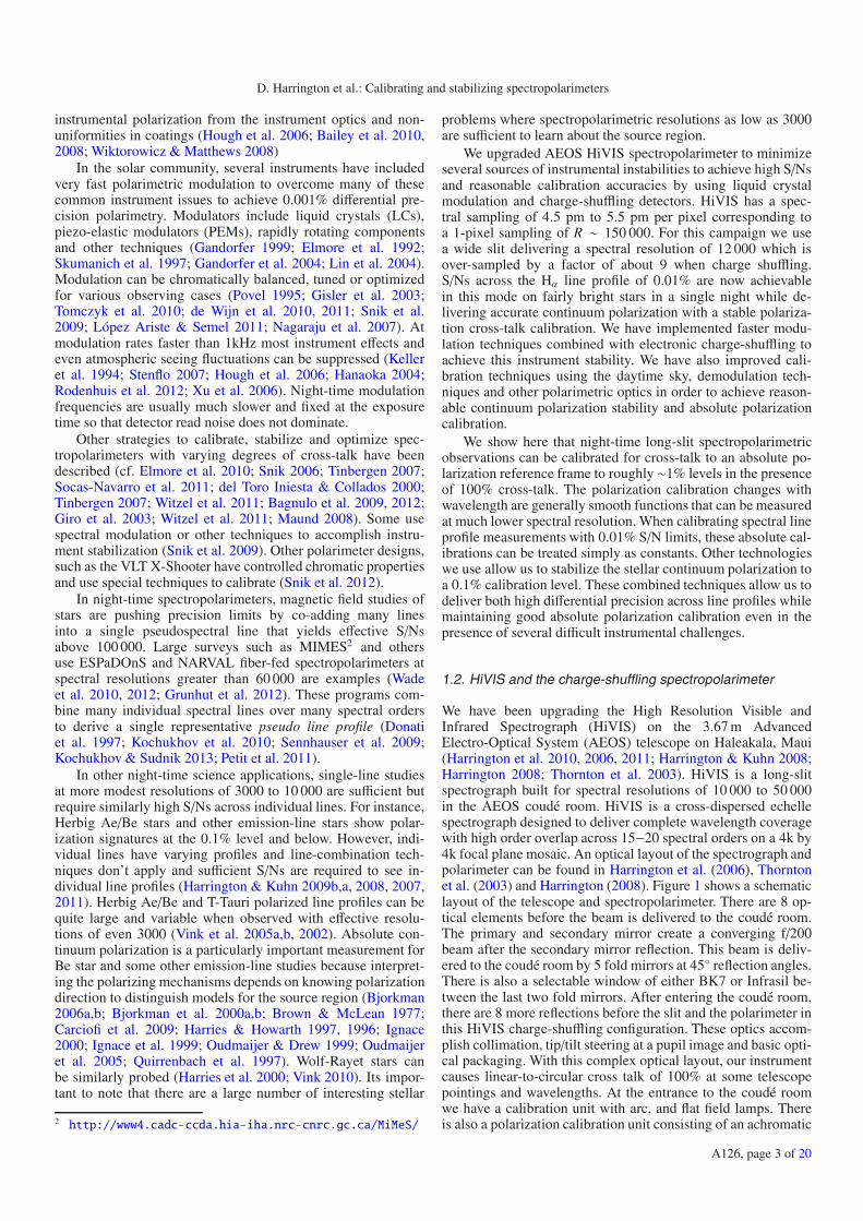
Fig. 10. Demodulated daytime sky polarization spectra on May 5th2012. The telescope pointing was azimuth 360 and elevation 90. Datawas taken at two different times (2.62 and 4.86 h UT). Each measure-ment has two independent demodulation calibrations applied with thetwo calibration unit demodulation matrices. The curves largely over-lap showing minimal chromatic effects from the polarization calibrationunit. Spectral averaging by a factor of 32 was applied to 125 data pointsper spectral order to achieve high S/N. The consistency of the data in-side each spectral order as well as agreement in regions of spectral orderoverlap is seen in the smooth spectral variation of the quv spectra.

at speeds of 1 Hz give stable measurements of both polarizedand unpolarized standard stars below 0.1% precision levels whenspectrally binned to high S/Ns. This system substantially re-duces the types of instrumental effects when comparing multiplelines across the spectrum. We find that relatively slow modula-tion rates combined with accurate guiding are sufficient to stabi-lize the optical path of the instrument and remove effects frompointing jitter.

3. Calibrations: daytime sky validation

Measuring absolute polarization with HiVIS requires a full-Stokes polarization calibration process to account for all the tele-scope and instrument induced cross-talk. In coudé path instru-ments and complex systems, this absolute calibration is oftenthe most unstable and difficult. The daytime sky is a very bright,highly polarized and easily modeled calibration source. It pro-vides linear polarization at any telescope pointing, has similarsurface brightness to bright stellar targets and does not wastenight time observing. We have developed techniques to observethe daytime sky polarization on our low resolution spectrograph,LoVIS in order to derive polarization calibrations for the tele-scope and instrument (Harrington et al. 2011). In Harringtonet al. (2010) we presented initial calibrations of the HiVIS liq-uid crystal polarimeter. Here we have successfully applied thisdaytime sky techniques to HiVIS and the liquid crystal de-modulation algorithms to our new charge shuffling instrument.Simple procedures can project these measurements to all tele-scope pointings and calibrate science observations.

In order to derive the polarization calibrations and the systemMuller matrix, full-Stokes observations must be obtained of thedaytime sky polarization spectra over a span of typically a fewhours. To obtain demodulation matrices, observations of calibra-tion lamps taken with our polarization calibration injection unitare also recorded and processed. This unit consists of a rotatingwire grid polarizer and a rotating achromatic quarter wave plate.

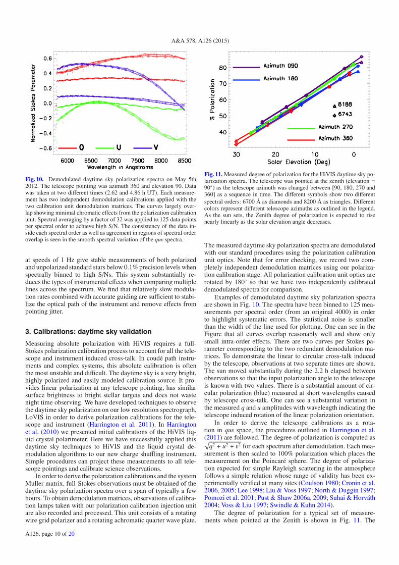
Fig. 11. Measured degree of polarization for the HiVIS daytime sky po-larization spectra. The telescope was pointed at the zenith (elevation =90◦) as the telescope azimuth was changed between [90, 180, 270 and360] as a sequence in time. The different symbols show two differentspectral orders: 6700 Å as diamonds and 8200 Å as triangles. Differentcolors represent different telescope azimuths as outlined in the legend.As the sun sets, the Zenith degree of polarization is expected to risenearly linearly as the solar elevation angle decreases.

The measured daytime sky polarization spectra are demodulatedwith our standard procedures using the polarization calibrationunit optics. Note that for error checking, we record two com-pletely independent demodulation matrices using our polariza-tion calibration stage. All polarization calibration unit optics arerotated by 180◦ so that we have two independently calibrateddemodulated spectra for comparison.

Examples of demodulated daytime sky polarization spectraare shown in Fig. 10. The spectra have been binned to 125 mea-surements per spectral order (from an original 4000) in orderto highlight systematic errors. The statistical noise is smallerthan the width of the line used for plotting. One can see in theFigure that all curves overlap reasonably well and show onlysmall intra-order effects. There are two curves per Stokes pa-rameter corresponding to the two redundant demodulation ma-trices. To demonstrate the linear to circular cross-talk inducedby the telescope, observations at two separate times are shown.The sun moved substantially during the 2.2 h elapsed betweenobservations so that the input polarization angle to the telescopeis known with two values. There is a substantial amount of cir-cular polarization (blue) measured at short wavelengths causedby telescope cross-talk. One can see a substantial variation inthe measured q and u amplitudes with wavelength indicating thetelescope induced rotation of the linear polarization orientation.

In order to derive the telescope calibrations as a rota-tion in quv space, the procedures outlined in Harrington et al.(2011) are followed. The degree of polarization is computed as√

q2 + u2 + v2 for each spectrum after demodulation. Each mea-surement is then scaled to 100% polarization which places themeasurement on the Poincaré sphere. The degree of polariza-tion expected for simple Rayleigh scattering in the atmospherefollows a simple relation whose range of validity has been ex-perimentally verified at many sites (Coulson 1980; Cronin et al.2006, 2005; Lee 1998; Liu & Voss 1997; North & Duggin 1997;Pomozi et al. 2001; Pust & Shaw 2006a, 2009; Suhai & Horváth2004; Voss & Liu 1997; Swindle & Kuhn 2014).

The degree of polarization for a typical set of measure-ments when pointed at the Zenith is shown in Fig. 11. The

A126, page 10 of 20

D. Harrington et al.: Calibrating and stabilizing spectropolarimeters

linearly increasing trend in degree of polarization is expected asthe scattering angle (sun-zenith-telescope) increases. The slightdifference in polarization between East (090) and North (360)azimuths reflects telescope depolarization as well as errors indemodulation. The measurements in Fig. 11 are consistent withthat Rayleigh sky model and a very high (85%) maximum de-gree of polarization. These values are typical and are similar toall-sky polarization measurements of Haleakala, Mauna-Loa ob-servatory, and other sites (Dahlberg et al. 2011, 2009; Swindle& Kuhn 2014). The high measured degree of polarization showsthat HiVIS with the liquid crystals and charge-shuffling onAEOS has little depolarization, certainly less than 5%. As withLoVIS and our other observing modes, observations of a wire-grid polarizer covering the calibration sources at the coudé roomentrance show polarization detected above 98% and high instru-ment detection efficiency.

3.1. Stability and accuracy of calibrations

Our daytime sky calibration technique only requires a mini-mum of two observations to derive a Mueller matrix estimate(Harrington et al. 2011). Additional observations provide redun-dant information that can be used to test systematic errors andimprove accuracy. Independent calibrations can be derived usingdata sub-sets to assess calibration systematic errors. A largedataset of daytime sky observations was recorded with HiVISusing charge-shuffling between April and June 2012 for verifi-cation. Calibrations were recorded at cardinal pointings (North,East, South and West azimuths) at elevations of 90◦, 70◦ and 55◦.We collected 4 to 9 measurements at many telescope pointingsand repeated observations over multiple epochs. For our statisti-cal analysis, we chose data sets with the telescope pointed at thezenith for the cardinal azimuths recorded on April 21st, 22nd andMay 10th 2012. For each observation date, an independent sys-tem Mueller matrix was computed following (Harrington et al.2011).

Since this calibration method effectively applies rotations onthe Poincaré sphere, we found it instructive to show the rota-tional error between the calibrated observations and the theoreti-cal daytime sky polarization. First we compute the demodulated,fully polarized observations. We then apply our three separatesystem Mueller-matrices to calibrate all the sky measurements.This gives us three sets of data calibrated using three indepen-dent system calibrations. The residual angular distance on thePoincaré sphere between these calibrated observations and thetheoretical Rayleigh sky polarization is computed for each wave-length and telescope pointing.

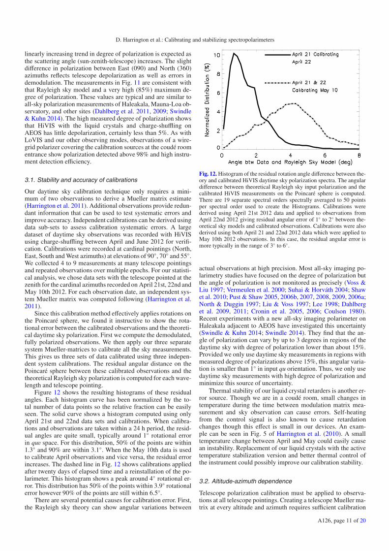
Figure 12 shows the resulting histograms of these residualangles. Each histogram curve has been normalized by the to-tal number of data points so the relative fraction can be easilyseen. The solid curve shows a histogram computed using onlyApril 21st and 22nd data sets and calibrations. When calibra-tions and observations are taken within a 24 h period, the resid-ual angles are quite small, typically around 1◦ rotational errorin quv space. For this distribution, 50% of the points are within1.3◦ and 90% are within 3.1◦. When the May 10th data is usedto calibrate April observations and vice versa, the residual errorincreases. The dashed line in Fig. 12 shows calibrations appliedafter twenty days of elapsed time and a reinstallation of the po-larimeter. This histogram shows a peak around 4◦ rotational er-ror. This distribution has 50% of the points within 3.9◦ rotationalerror however 90% of the points are still within 6.5◦.

There are several potential causes for calibration error. First,the Rayleigh sky theory can show angular variations between

Fig. 12. Histogram of the residual rotation angle difference between the-ory and calibrated HiVIS daytime sky polarization spectra. The angulardifference between theoretical Rayleigh sky input polarization and thecalibrated HiVIS measurements on the Poincaré sphere is computed.There are 19 separate spectral orders spectrally averaged to 50 pointsper spectral order used to create the Histograms. Calibrations werederived using April 21st 2012 data and applied to observations fromApril 22nd 2012 giving residual angular error of 1◦ to 2◦ between the-oretical sky models and calibrated observations. Calibrations were alsoderived using both April 21 and 22nd 2012 data which were applied toMay 10th 2012 observations. In this case, the residual angular error ismore typically in the range of 3◦ to 6◦.

actual observations at high precision. Most all-sky imaging po-larimetry studies have focused on the degree of polarization butthe angle of polarization is not monitored as precisely (Voss &Liu 1997; Vermeulen et al. 2000; Suhai & Horváth 2004; Shawet al. 2010; Pust & Shaw 2005, 2006b, 2007, 2008, 2009, 2006a;North & Duggin 1997; Liu & Voss 1997; Lee 1998; Dahlberget al. 2009, 2011; Cronin et al. 2005, 2006; Coulson 1980).Recent experiments with a new all-sky imaging polarimeter onHaleakala adjacent to AEOS have investigated this uncertainty(Swindle & Kuhn 2014; Swindle 2014). They find that the an-gle of polarization can vary by up to 3 degrees in regions of thedaytime sky with degree of polarization lower than about 15%.Provided we only use daytime sky measurements in regions withmeasured degree of polarizations above 15%, this angular varia-tion is smaller than 1◦ in input qu orientation. Thus, we only usedaytime sky measurements with high degree of polarization andminimize this source of uncertainty.

Thermal stability of our liquid crystal retarders is another er-ror source. Though we are in a coudé room, small changes intemperature during the time between modulation matrix mea-surement and sky observation can cause errors. Self-heatingfrom the control signal is also known to cause retardationchanges though this effect is small in our devices. An exam-ple can be seen in Fig. 5 of Harrington et al. (2010). A smalltemperature change between April and May could easily causean instability. Replacement of our liquid crystals with the activetemperature stabilization version and better thermal control ofthe instrument could possibly improve our calibration stability.

3.2. Altitude-azimuth dependence

Telescope polarization calibration must be applied to observa-tions at all telescope pointings. Creating a telescope Mueller ma-trix at every altitude and azimuth requires sufficient calibration

A126, page 11 of 20

A&A 578, A126 (2015)

Fig. 13. Six Mueller matrix estimates derived via our least-squaresmethod using all data from our 2013 to 2014 calibration efforts. Eachcolored point represents an altitude-azimuth telescope pointing wherewe have quality data for estimating the telescope Mueller matrix. TheQQ and QU terms are on top. The UQ and UU terms are in the middle.The QV and UV terms are on the bottom. Note the bottom row repre-sents linear to circular polarization cross-talk and the amplitudes are at100% for many pointings.

data to accurately characterize the behavior of the telescopeMueller matrix. An observing campaign was performed duringwinter of 2013 and summer of 2014 to make a densely coveredset of calibrations with HiVIS and charge shuffling. Daytime skypolarization observations were obtained in October, Novemberand December of 2013 as well as in May of 2014. We recordedmany redundant exposures at azimuths of [030, 060, 090, 120,150, 180, 210, 270, 330, 360]. The corresponding elevationswere: [10, 20, 25, 35, 50, 60, 75, 89]. Recent upgrades to theAEOS telescope now allow observations all day. Previously, ourtelescope pointing elevation limit was above 55◦ and the sun hadto be below elevations of 45◦.

The procedure outlined in Harrington et al. (2011) allowsone to estimate Mueller matrix elements from Rayleigh skyobservations. We scale all HiVIS daytime sky observations to100% degree of polarization before we calculate the cross-talkterms of the Mueller matrix. Measurements are put on to thePoincaré sphere before deriving the best-fit rotation matrices asthis results in constructing a physically realistic Mueller matrix.This procedure models telescope as a simple rotation incomingquv polarization to some other quv basis set. As an example ofthe altitude-azimuth behavior, we show the Mueller matrix esti-mates for spectral order 3 in Fig. 13.

For AEOS, the functional dependence with altitude and az-imuth follows simple trigonometric functions and can be fit witha few independent parameters. The dominant polarization cross-talk is caused by rotation of the fold mirrors along the altitudeand azimuthal axes. With simple functional coefficients, we canre-compute the azimuthal dependence at an arbitrary telescopepointing. Figure 17 shows the result of this interpolation. Thecross-talk elements of the telescope Mueller matrix are shownfor all altitudes and azimuths. This process allows individualMueller matrix elements to be obtained at the pointing of theastronomical target. After interpolation, the user can derive the

Fig. 14. Cumulative error distribution functions when fitting rotationmatrix functions of azimuth and elevation to the individual mueller ma-trix elements. The distribution is based on the difference between thebest-fit rotation matrix and each individual least-squares based Muellermatrix estimate at every measured azimuth and elevation. Each colorcorresponds to one of the six Mueller matrix estimates computed usingour daytime sky method. The 68% confidence interval falls betweenerrors of 0.04 for some elements and 0.10 for other elements.

best-fit rotation matrix using the standard Euler-angle procedureoutlined in Harrington et al. (2011). This ensures physicalityof the telescope Mueller matrix and reduces errors in Muellermatrix term estimation. By representing the telescope Muellermatrix as a rotation matrix, we ensure physicality of the trans-formation and we do not amplify certain kinds of systematicnoise (Kostinski et al. 1993; Takakura & Stoll 2009; Givens &Kostinski 1993).

To quantify the errors, we derive the cumulative distributionfunction for the difference between the six independent Muellermatrix estimates and the corresponding best-fit rotation matri-ces after applying the altitude-azimuth interpolation. Figure 14shows each Mueller matrix estimate in a different color. Thetrigonometric function fitting results in an uncertainty of lessthan 0.1 between the estimates and the rotation matrix fits.

One of the major sources of calibration uncertainty in thepresent approach is the stability of the liquid crystals in tem-perature and time. The individual measurements can calibratedand differenced from the theoretical daytime sky polarization todemonstrate the demodulation and cross-talk calibration errors.Figure 15 shows the difference between the theoretical Rayleighsky polarization spectra and demodulated calibrated HiVIS mea-surements. In this Figure, April 21st 2012 data was used toderive Euler angles. This data was then polarization calibratedand subtracted from the theoretical Rayleigh sky polarization.The residual errors are typically less than 0.05 in any individ-ual Stokes parameter. These residual errors were used to derivea rotational measure of absolute calibration accuracy and are thebasis for the histograms of the angle between the measured cali-brated Stokes vector and the theoretical daytime sky Stokes vec-tor shown above in Fig. 12.

We find that the likely cause of the ripples seen at smallwavelength scales within individual spectral orders is causedby slight changes in liquid crystal properties. In Fig. 3 ofHarrington et al. (2010), we showed a transmission function us-ing a very small beam footprint using a Varian spectrophotome-ter. This Varian is effectively a lab-calibrated commercial scan-ning monochrometer. This instrument also showed small-scaleripples in the overall transmission function that were highly de-pendent on placement of the liquid crystal. Similar ripples were

A126, page 12 of 20

D. Harrington et al.: Calibrating and stabilizing spectropolarimeters

Fig. 15. Difference between the demodulated and calibrated Stokes parameters and the predicted Rayleigh sky polarization spectra forApril 21st 2012. Each panel shows observations calibrated at a different telescope azimuth. There are 4 to 5 independent observations at eachtelescope pointing. Different colors represent residual Stokes parameters for individual observations computed as data minus model. The residualsare always below 0.1 across the wavelength range. Note – only a single calibration point per spectral order has been applied and the data is shownbinned to 50 spectral samples per order. Note that these residual Stokes parameters give rise to the few degree rotational error between a measuredStokes vector and a model Stokes vector projected on the Poincar’e sphere as shown above in Fig. 12.

seen in Fig. 5 of Harrington et al. (2010) when the temper-ature of the device was changed. Liquid crystal stability willlikely be a limitation of our system. We note that the calibra-tions applied here only use one telescope Mueller matrix elementper spectral order. Potentially performing calibrations with moredata at higher spectral sampling could improve the calibrationprocedures.

The wavelength dependence of the telescope Mueller matrixis very slow. Figure 16 shows the six Mueller matrix estimatesafter being fit to simple trigonometric functions of altitude andazimuth. The top panel shows the 6225 Å spectral order whilethe bottom panel shows the 8601 Å spectral order. The linearpolarization terms are dominated by the transformation betweenan altitude-azimuth based frame and a Zenith frame. The circularpolarization terms are quite strong at 6225 Å but tend towardszero at 8601 Å. Given this gradual wavelength dependence, wefind that one calibration per spectral order is sufficient for thisdemonstration.

3.3. Example calibration of ε Aurigae

Epsilon Aurigae is a very bright target with a known strong andvariable Hα polarization signature (Harrington & Kuhn 2009a;Kemp et al. 1986, 1985; Cole & Stencel 2011; Hall & Henson2010; Henson et al. 2012; Burdette & Henson 2012; Stencel2013). We have a long and detailed set of ε Aur observationstaken with ESPaDOnS at CFHT for comparison. We have neverdetected any circular polarization in Hα in the 2006 to 2012time frame. As an example of this stars Hα line profile, we com-piled 42 independent measurements in to blocks where the targetshows substantially different polarization and intensity line pro-files. Figure 18 shows the observations broken in to 9 main ob-serving blocks covering summer and winter observing seasonsover the 6 years. We followed our recipe for post-processing ofthe Libre-Esprit reduced ESPaDONs spectra outlined in the ap-pendix of Harrington et al. (2009). Essentially our process com-bines the reduced spectra from individual spectral orders and av-erages pixels to a more uniform spectral sampling. In the caseof Fig. 18 the effective spectral sampling is at about 35 pm per

pixel for a 1-point sampling of R ∼ 170 000 data. For the pur-poses of this calibration we note that the polarized Hα profileshave amplitudes of 0.5% up to 1% while Stokes v signatures areundetectable to within the S/N thresholds. The effective S/Ns inboth the ESPaDOnS data sets is over 1000 per pixel and the rele-vant spectral features are very broad. Our HiVIS charge-shuffledspectra are sampled at ∼44 pm per pixel at Hα and we highlyover-sample the delivered optical resolution of 12 000 to achievehigh S/Ns efficiently on bright targets.

During October 23, 2013, a large set of observations wererecorded on the star ε Aurigae while performing our daytimesky calibration mapping procedures. We collected 30 individualpolarization measurements over the course of one night. Over theobservations, azimuths ranged from 055◦ through transit to 330◦.Elevations were between 34◦ and 67◦. Each full-Stokes ε Aurobservation set was reduced and demodulated using the standardobserving sequence with our polarization calibration unit. TheS/N for each individual quv measurement was between 650 and900 for all 30 independent quvmeasurements.

There were 4 separate clusters of data recorded at telescopepointings of (051, 35), (045, 52), (011, 67) and (333, 64). Thereare 5, 10, 5 and 10 consecutive exposures in each of the associ-ated observing blocks. Figure 19 shows the quv spectra averagedduring these 4 observing blocks. The ESPaDOnS spectra showthat the Hα signature is always contained entirely in linear po-larization qu. However, since the linear to circular cross-talk is100% at some telescope pointings for HiVIS, our uncalibrateddata shows this Hα signature largely in Stokes v. Some changescan be seen in the details of the quv profiles, showing the chang-ing cross-talk as the telescope tracks the star.

Using the telescope Mueller matrix element estimates, thebest-fit rotation-matrix was computed for the telescope pointingat each ε Aurigae data set following our procedures (Harringtonet al. 2011). The telescope Mueller matrix maps of Fig. 17 can beinterpolated to the telescope pointing of every individual obser-vation. Figure 20 shows the telescope Mueller matrix estimatesfor every individual observation of ε Aurigae. The 4 observingblocks can be seen as clusters of points with similar Muellermatrix elements. For example, the far right side of Fig. 20 shows

A126, page 13 of 20

A&A 578, A126 (2015)

Fig. 16. Six Mueller matrix estimates trigonometry function fitting forall altitudes and azimuths. The QQ and QU terms are on top. The UQand UU terms are in the middle. The QV and UV terms are on thebottom. The top graphic shows spectral order at 6225 Å. The bottomgraphic shows spectral order at 8601 Å with much reduced circular po-larization cross-talk (low QV and UV values). The sinusoidal variationin the linear polarization terms represent the transformation between thealtitude-azimuth frame and a Zenith based polarization frame.

a cluster of 5 observations while ε Aurigae was rising at (az-imuth, elevation) of (051, 35). The telescope pointing changeduring this time was largely elevation. On the far left side ofFig. 20, a sequence of 10 observations is seen near an (az-imuth,elevation) of (333, 64) while the predominant telescopepointing change was in azimuth.

These telescope Mueller matrix calibrations were applied toeach ε Aurigae data set. Figure 21 shows the average demodu-lated and calibrated data sets for the 4 major observing blocks.The top three panels show Stokes q, u and v respectively. Thebottom panel shows the continuum-normalized intensity profilefor Hα. The uncalibrated measurements showed the observedsignature was dominantly Stokes v with substantial q and u.

After applying the telescope calibrations, the Hα line profile sig-nature is almost entirely contained in Stokes q and u.

There are several sources of error in these demonstrationcalibrations that can easily be improved. First, we have onlyused one calibration per spectral order which gives some mildwavelength dependent residual errors across a spectral order.Secondly, the daytime sky observations were recorded over a6 month time frame. This leads to several degrees rotational er-rors as seen in the histogram of Fig. 12. Note that a Stokes pa-rameter error of 0.05 corresponds to a 3◦ misalignment whilea 0.2 error corresponds to an 11◦ misalignment. Since we onlyapply one calibration per spectral order, for an effective reduc-tion in wavelength sampling by a factor of 4000, we get resid-ual errors wavelength from the liquid crystal ripples and generalwavelength dependent behavior as seen in Fig. 15. The third er-ror comes from interpolating the best-fit rotation matrix to thetelescope pointings of every individual observation. The cumu-lative distribution functions of Fig. 14 show that the Mueller ma-trix element fitting process gives 1σ errors at element values ofroughly 0.04 to 0.10 for a 68% error level. This corresponds toadditional rotational error levels of 2◦ to 6◦.

The calibrated quv behavior for ε Aurigae is shown inFig. 22. To show the quv behavior at high signal to shot-noise ra-tios, we combined all individual calibrated spectra and then aver-aged 4 pixels in the spectral direction. The S/N of these averagespectra is between 5700 and 7700 as estimated from the standarddeviation of the noise of the continuum adjacent to the Hα line.After the 4-pixel averaging, we sample our R ∼ 12 000 spectraat an effective sampling of 34 000 for 3 points per resolution el-ement. The residual Stokes v signature in Fig. 21 is expected isan amplitude of 0.14% while the qu amplitude is at 0.50%. Thiscorresponds to a misalignment of 15.6◦. As shown in Fig. 12,we expect leakage of this magnitude considering all the instru-ment changes in the long time span between calibrations andobservations.

4. Conclusions

We have demonstrated here general techniques that overcomeboth calibration-type uncertainties (I) and measurement stabil-ity issues (II). S/Ns above 0.01% were achieved at full spectralresolution using calibration sources. On-sky calibrated observa-tions of ε Aurigae achieved S/Ns of 5000 to 7600 at R = 34 000sampling. Using our new daytime sky calibration technique, wehave independently calibrated the polarization response of theinstrument and telescope as functions of altitude and azimuthin a system with 100% cross talk. In this altitude-azimuth tele-scope the polarization cross-talk calibration has a simple func-tional form on-sky and can be done easily on a routine basis toassure calibration stability. The cross-talk calibration was testedon a stellar target ε Aurigae with good results. Several sources ofcalibration algorithm uncertainty have been identified and futureimprovements are expected.

The quality of our cross-talk calibration method was shownto be better than 4% in an individual Stokes parameter if cali-brations are taken within a day of the observations at the sametelescope pointing. This corresponds to a 2◦ Poincare-sphere ro-tational uncertainty of the polarization orientation. Calibrationstaken even a month after observations still provide 5◦ rota-tional accuracy which corresponds to about 10% of an individ-ual Stokes parameter. Our assumptions of a weakly depolariz-ing our telescope and instrument are reasonable given the degreeof polarization measured for polarized standard stars as well as

A126, page 14 of 20

D. Harrington et al.: Calibrating and stabilizing spectropolarimeters

Fig. 17. Altitude-azimuth map of the system Mueller matrix cross-talk elements for the 6560 Å spectral order. The best fit rotation matrix was fitto the Mueller matrix estimates elements following our standard procedure. The Mueller matrix element az-el maps are all linearly scaled fromblack at −1 to white at +1. Each element is plotted from the horizon to the Zenith for the full 360◦ azimuth range.

Fig. 18. ε Aurigae Hα line profiles observed with ESPaDOnS between2006 and 2012. This star has shown strong variable qu profiles butStokes vwas always zero within the statistical noise. See text for details.

for the high measured daytime sky degree of polarization maxi-mum (δmax).

We were able to measure both polarized standard stars andunpolarized standard stars with smooth reproducible continuumpolarization at the 0.1% level even in the presence of a >2%inter-order artifact. We applied firmware and software upgradesto accomplish charge shuffling with a CCD that was not origi-nally designed for this purpose. Many of our instrument stability

Fig. 19. Average quv data sets in 4 main telescope pointing blocks forε Aurigae observed with HiVIS on October 23rd 2013. No telescopeMueller matrix calibration has been applied. The input signal is qu asshown by ESPaDOnS observations but the detected HiVIS signatureis much larger in v due to the telescope cross-talk. The 4 independentquv spectra show some spectral variation due to changes in the telescopecross-talk as the optics change with time. See text for details.

issues (Type II) were overcome while improving our measure-ment efficiency. This new combination of charge shuffling, liq-uid crystal modulation and daytime sky calibration can delivercalibrated, high precision observations for use in a variety of

A126, page 15 of 20

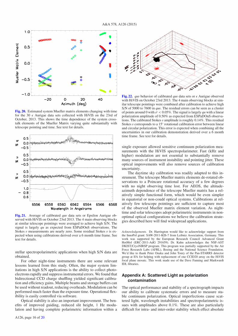
A&A 578, A126 (2015)

Fig. 20. Estimated system Mueller matrix elements changing with timefor the 30 ε Aurigae data sets collected with HiVIS on the 23rd ofOctober, 2013. This shows the time dependence of the system cross-talk elements of the Mueller Matrix varying quite substantially withtelescope pointing and time. See text for details.

Fig. 21. Average of calibrated quv data sets or Epsilon Aurigae ob-served with HiVIS on October 23rd 2013. The 4 main observing blocksat similar telescope pointings were averaged to achieve high S/N. Thesignal is largely qu as expected from ESPaDOnS observations. TheStokes v measurements are nearly zero. Some residual Stokes v is ex-pected when using calibrations derived over a 6 month time frame. Seetext for details.

stellar spectropolarimetric applications when high S/N data areobtained.

For other night-time instruments there are some relevantlessons learned from this study. Often, the major system lim-itations in high S/N applications is the ability to collect photo-electrons rapidly and suppress instrumental errors. We found thatbidirectional CCD charge shuffling yielded significant calibra-tion and efficiency gains. Multiple beams and storage buffers canbe used without readout, reducing overheads. Modulation can beperformed much faster than the exposure time. Operational flex-ibility is easily controlled via software.

Optical stability is also an important improvement. The ben-efits of improved guiding, reduced slit height, 1 Hz modu-lation and having complete polarimetric information within a

Fig. 22. quv behavior of calibrated quv data sets or ε Aurigae observedwith HiVIS on October 23rd 2013. The 4 main observing blocks at sim-ilar telescope pointings were combined after calibration to achieve highS/N of 5000 to 7600 in quv. The residual errors can be seen as a clusterof points around 0 withσ < 0.05%. The signal is largely qu with a linearpolarization amplitude of 0.50% as expected from ESPaDOnS observa-tions. The calibrated Stokes v amplitude is roughly 0.14%. This residualStokes v corresponds to a 15◦ rotational calibration error between linearand circular polarization. This error is expected when combining all theuncertainties in our calibration demonstration derived over a 6 monthtime frame. See text for details.

single exposure allowed sensitive continuum polarization mea-surements with the HiVIS spectropolarimeter. Fast (kHz andhigher) modulation are not essential to substantially removemany sources of instrument instability and pointing jitter. Theseoptical improvements will also remove sources of calibrationuncertainty.

The daytime sky calibration was readily adapted to this in-strument. The telescope Mueller matrix elements de-rotated ob-servations to a Poincare rotational accuracy of a few degreeswith no night observing time lost. For AEOS, the altitude-azimuth dependence of the telescope Mueller matrix has a rel-atively simple functional form, which would be even simplerin equatorial or non-coudé optical systems. Calibrations at rel-atively few telescope pointings are sufficient to capture mostof the observed Mueller matrix element variation. As night-time and solar telescopes adopt polarimetric instruments in non-optimal optical configurations we believe the calibration strate-gies described here will find widespread applications.

Acknowledgements. Dr. Harrington would like to acknowledge support fromthe InnoPol grant: SAW-2011-KIS-7 from Leibniz Association, Germany. Thiswork was supported by the European Research Council Advanced GrantHotMol (ERC-2011-AdG 291659). Dr. Kuhn acknowledges the NSF-ASTDKIST/CryoNIRSP program. This program was partially supported by the AirForce Research Labs (AFRL), Boeing and the National Science Foundation.We’d like to thank Peter Onaka and John Tonry of the Pan-STARRS detectorgroup at IfA for helping with replacement of one CCID20 array on the HiVISfocal plane mosaic. This work made use of the Dave Fanning and MarkwardtIDL libraries.

Appendix A: Scattered Light as polarizationcontamination

The optical performance and stability of a spectrograph impactsour ability to calibrate systematic errors and to measure sta-ble continuum polarization. Optical imperfections cause scat-tered light, wavelength instabilities and spectropolarimetric is-sues with amplitudes above 0.1%. These are also particularlydifficult for intra- and inter-order stability which effect absolute

A126, page 16 of 20

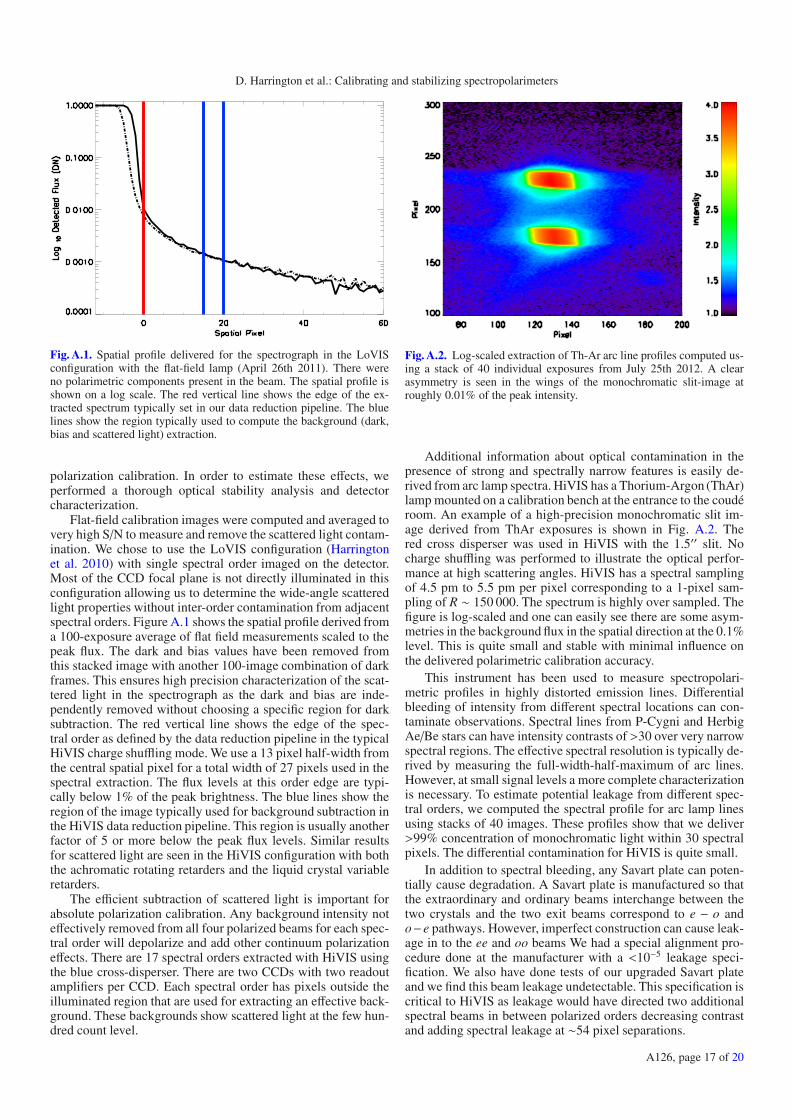
D. Harrington et al.: Calibrating and stabilizing spectropolarimeters

Fig. A.1. Spatial profile delivered for the spectrograph in the LoVISconfiguration with the flat-field lamp (April 26th 2011). There wereno polarimetric components present in the beam. The spatial profile isshown on a log scale. The red vertical line shows the edge of the ex-tracted spectrum typically set in our data reduction pipeline. The bluelines show the region typically used to compute the background (dark,bias and scattered light) extraction.

polarization calibration. In order to estimate these effects, weperformed a thorough optical stability analysis and detectorcharacterization.

Flat-field calibration images were computed and averaged tovery high S/N to measure and remove the scattered light contam-ination. We chose to use the LoVIS configuration (Harringtonet al. 2010) with single spectral order imaged on the detector.Most of the CCD focal plane is not directly illuminated in thisconfiguration allowing us to determine the wide-angle scatteredlight properties without inter-order contamination from adjacentspectral orders. Figure A.1 shows the spatial profile derived froma 100-exposure average of flat field measurements scaled to thepeak flux. The dark and bias values have been removed fromthis stacked image with another 100-image combination of darkframes. This ensures high precision characterization of the scat-tered light in the spectrograph as the dark and bias are inde-pendently removed without choosing a specific region for darksubtraction. The red vertical line shows the edge of the spec-tral order as defined by the data reduction pipeline in the typicalHiVIS charge shuffling mode. We use a 13 pixel half-width fromthe central spatial pixel for a total width of 27 pixels used in thespectral extraction. The flux levels at this order edge are typi-cally below 1% of the peak brightness. The blue lines show theregion of the image typically used for background subtraction inthe HiVIS data reduction pipeline. This region is usually anotherfactor of 5 or more below the peak flux levels. Similar resultsfor scattered light are seen in the HiVIS configuration with boththe achromatic rotating retarders and the liquid crystal variableretarders.

The efficient subtraction of scattered light is important forabsolute polarization calibration. Any background intensity noteffectively removed from all four polarized beams for each spec-tral order will depolarize and add other continuum polarizationeffects. There are 17 spectral orders extracted with HiVIS usingthe blue cross-disperser. There are two CCDs with two readoutamplifiers per CCD. Each spectral order has pixels outside theilluminated region that are used for extracting an effective back-ground. These backgrounds show scattered light at the few hun-dred count level.

Fig. A.2. Log-scaled extraction of Th-Ar arc line profiles computed us-ing a stack of 40 individual exposures from July 25th 2012. A clearasymmetry is seen in the wings of the monochromatic slit-image atroughly 0.01% of the peak intensity.

Additional information about optical contamination in thepresence of strong and spectrally narrow features is easily de-rived from arc lamp spectra. HiVIS has a Thorium-Argon (ThAr)lamp mounted on a calibration bench at the entrance to the coudéroom. An example of a high-precision monochromatic slit im-age derived from ThAr exposures is shown in Fig. A.2. Thered cross disperser was used in HiVIS with the 1.5′′ slit. Nocharge shuffling was performed to illustrate the optical perfor-mance at high scattering angles. HiVIS has a spectral samplingof 4.5 pm to 5.5 pm per pixel corresponding to a 1-pixel sam-pling of R ∼ 150 000. The spectrum is highly over sampled. Thefigure is log-scaled and one can easily see there are some asym-metries in the background flux in the spatial direction at the 0.1%level. This is quite small and stable with minimal influence onthe delivered polarimetric calibration accuracy.

This instrument has been used to measure spectropolari-metric profiles in highly distorted emission lines. Differentialbleeding of intensity from different spectral locations can con-taminate observations. Spectral lines from P-Cygni and HerbigAe/Be stars can have intensity contrasts of >30 over very narrowspectral regions. The effective spectral resolution is typically de-rived by measuring the full-width-half-maximum of arc lines.However, at small signal levels a more complete characterizationis necessary. To estimate potential leakage from different spec-tral orders, we computed the spectral profile for arc lamp linesusing stacks of 40 images. These profiles show that we deliver>99% concentration of monochromatic light within 30 spectralpixels. The differential contamination for HiVIS is quite small.

In addition to spectral bleeding, any Savart plate can poten-tially cause degradation. A Savart plate is manufactured so thatthe extraordinary and ordinary beams interchange between thetwo crystals and the two exit beams correspond to e − o ando−e pathways. However, imperfect construction can cause leak-age in to the ee and oo beams We had a special alignment pro-cedure done at the manufacturer with a <10−5 leakage speci-fication. We also have done tests of our upgraded Savart plateand we find this beam leakage undetectable. This specification iscritical to HiVIS as leakage would have directed two additionalspectral beams in between polarized orders decreasing contrastand adding spectral leakage at ∼54 pixel separations.

A126, page 17 of 20

A&A 578, A126 (2015)

Fig. A.3. Computed spatial profile for the spectral order 10 with a widedekker setting. This wide dekker exaggerates the intra-order contam-ination. There were no modulators in the beam. Charge shuffling of27 pixels was done with polarization calibration unit polarizer in place.Beams a and b represent one set of orthogonally polarized spectra.Beams c and d represent another set of orthogonally polarized spectra.The asymmetry in intra-order contamination is easily seen where in-tense d and b beams strongly influence c but not a. In double-differencedpolarization calculations, this leads to spurious continuum polarizationeffects.

The spatial width of the extracted spectra combined with theslit dekker width and any optical imperfections will cause intra-order contamination between modulated beams. This will cre-ate a systematic continuum polarization error when doing chargeshuffling. The light that bleeds from one modulation state withpolarization (a − b/a + b) in to the other modulation state withpolarization (c − d/c + d) asymmetrically will cause continuumvariations. As an illustration of this effect, Fig. A.3 shows thefour beams for the 10th spectral order for HiVIS on May 25th2010. In order to exaggerate the typical continuum effects, theslit dekker was set wider than nominal. The modulators (liquidcrystals and rotating retarders) were removed to ensure that scat-tered light was the dominant error.

One can see in Fig. A.3 that the asymmetric bleeding of onebeam in to the other will cause different computed intensitieseven though no modulation or optical movement was present.The incomplete separation of beams lead to a systematic de-crease in the detected degree of polarization for each of theHiVIS orders as well as an increase in the systematic error acrosseach individual order. The b and d beams had similar intensityand similar bleeding so these spectra were influenced little. Thec spectra was much more substantially influenced because ofit’s low intensity (300 counts) and the proximity to the brightb spectrum. The uneven disruption of the a and c spectra causeda much more substantial error in the (c − d)/(c + d) polarizationmeasurement.

In typical double difference calculations, the two methods donot give the same continuum polarization. The two methods inthis nomenclature are:

qab−cd =QI=

12

(a − ba + b

− c − dc + d

)(A.1)

and

qac−bd =QI=

12

(a − ca + c

− b − db + d

)· (A.2)

Fig. A.4. Derived Stokes q continuum polarization with HiVIS usingthe polarization calibration unit and only the Savart plate analyzer. Nomodulators were present in the optical beam. The asymmetry betweenthe (a-b) beams and (c-d) beams can be readily traced to the inter-beamcontamination when strongly polarized signals are present.

Without asymmetries in the optics, detector and modulation,these two equations should give identical results. In Harrington& Kuhn (2008) this is exactly what we find for HiVIS with onlytwo well separated beams. The qab calculation does a normalizedratio with spectra recorded simultaneously in time. The qac cal-culation is a normalized ratio with spectra recorded on the samepixel for gain independence but with temporal changes betweenbeams possible. If these four beams are not well separated andstable in time and completely unpolarized at the analyzer, con-tinuum polarization errors will be present. As a demonstration,Fig. A.4 shows the computed polarization for this May 2010 ex-periment with the flat field calibration lamps. Since the mod-ulators were removed and no optical motion occurred betweenmodulation states, the derived Stokes q polarization should benearly 100% and identical between the ab and cd calculations.Figure A.4 shows that the ab spectra have a very different con-tamination than the cd spectra across individual spectral ordersat the 0.5% level.

These asymmetries combined with typical optical instabili-ties (pointing, guiding, seeing, etc.) conspire to add systematiccontinuum variations across spectral orders that are difficult tocalibrate. This is a major limitation when stabilizing the contin-uum polarization of a slit spectropolarimeter.

ReferencesBagnulo, S., Szeifert, T., Wade, G. A., Landstreet, J. D., & Mathys, G. 2002,

A&A, 389, 191Bagnulo, S., Landolfi, M., Landstreet, J. D., et al. 2009, PASP, 121, 993Bagnulo, S., Landstreet, J. D., Fossati, L., & Kochukhov, O. 2012, A&A, 538,

A129Bailey, J., Ulanowski, Z., Lucas, P. W., et al. 2008, MNRAS, 386, 1016Bailey, J., Lucas, P. W., & Hough, J. H. 2010, MNRAS, 405, 2570Barrick, G., & Benedict, T. 2010, in SPIE Astronomical Telescopes and

Instrumentation: Observational Frontiers of Astronomy for the New Decade,ed. I. S. McLean, S. K. Ramsay, & H. Takami (SPIE), 773548

Barrick, G., Benedict, T., & Sabin, D. 2010, in SPIE Astronomical Telescopesand Instrumentation: Observational Frontiers of Astronomy for the NewDecade, eds. I. S. McLean, S. K. Ramsay, & H. Takami (SPIE), 77354

Bjorkman, J. E. 2006a, in Stars with the B[e] Phenomenon, ASP Conf. Ser., 355,231

Bjorkman, K. S. 2006b, in Stars with the B[e] Phenomenon, ASP Conf. Ser.,355, 247

A126, page 18 of 20

D. Harrington et al.: Calibrating and stabilizing spectropolarimeters

Bjorkman, K. S., & Meade, M. R. 2005, Astronomical Polarimetry: CurrentStatus and Future Directions ASP Conf. Ser., 343, 406

Bjorkman, K. S., Bjorkman, J. E., & Wood, K. 2000a, The Be Phenomenon inEarly-Type Stars, 214, 603

Bjorkman, K. S., Meade, M. R., & Babler, B. L. 2000b, The Be Phenomenon inEarly-Type Stars, 214, 48

Brown, J. C., & McLean, I. S. 1977, A&A, 57, 141Burdette, J. A., & Henson, G. D. 2012, J. Southeastern Association for Research

in Astronomy, 5, 51Burke, B. E., Tonry, J. L., Cooper, M. J., et al. 2007, Sensors, 6501, 6Carciofi, A. C., Okazaki, A. T., Le Bouquin, J.-B., et al. 2009, A&A, 504, 915Cole, G. M., & Stencel, R. E. 2011, The Society for Astronomical Sciences 30th

Annual Symposium on Telescope Science, Held May 24–26, 30, 103Coulson, K. L. 1980, Appl. Opt., 19, 3469Cronin, T. W., Warrant, E. J., & Greiner, B. 2005, Polarization Science and

Remote Sensing II, 5888, 204Cronin, T. W., Warrant, E. J., & Greiner, B. 2006, Appl. Opt. IP, 45, 5582Dahlberg, A. R., Pust, N. J., & Shaw, J. A. 2009, in SPIE, 7461, 6Dahlberg, A. R., Pust, N. J., & Shaw, J. A. 2011, Opt. Exp., 19, 16008de Juan Ovelar, M., Snik, F., & Keller, C. U. 2011, Proc. SPIE, 8160, 81600de Juan Ovelar, M., Diamantopoulou, S., Roelfsema, R., et al. 2012, in Modeling,

Systems Engineering and Project Management for Astronomy, Proc. SPIE,8449, 844912

de Wijn, A. G., Tomczyk, S., Casini, R., & Nelson, P. G. 2010, Proc. SPIE, 7735,77354

de Wijn, A. G., Tomczyk, S., Casini, R., & Nelson, P. G. 2011, in SolarPolarization, eds. J. R. Kuhn, D. M. Harrington, H. Lin, et al., Proc. ASP,437, 413

de Wijn, A. G., Casini, R., Nelson, P. G., & Huang, P. 2012, Proc. SPIE, 8446,84466

del Toro Iniesta, J. C., & Collados, M. 2000, App. Opt., 39, 1637Donati, J.-F., Semel, M., Carter, B. D., Rees, D. E., & Collier Cameron, A. 1997,

MNRAS, 291, 658Donati, J.-F., Catala, C., Wade, G. A., et al. 1999, A&A, 134, 149Elmore, D. F., Lites, B. W., Tomczyk, S., et al. 1992, in Polarization analysis

and measurement, Proceedings of the Meeting, High Altitude Observatory,Boulder, CO, 22

Elmore, D. F., Lin, H., Socas Navarro, H., & Jaeggli, S. A. 2010, in SPIE, 7735,147

Eversberg, T., Moffat, A. F. J., Debruyne, M., et al. 1998, PASP, 110, 1356Fossati, L., Bagnulo, S., Mason, E., & Landi Degl’Innocenti, E. 2007, The Future

of Photometric, ASP Conf. Ser., 364, 503Gandorfer, A. M. 1999, Opt. Eng., 38, 1402Gandorfer, A. M., Steiner, H. P. P. P., Aebersold, F., et al. 2004, A&A, 422, 703Gehrels, T. 1974, in Planets, Stars and Nebulae Studied with Photopolarimetry

(Tucson: University of Arizona Press)Gil-Hutton, R., & Benavidez, P. 2003, MNRAS, 345, 97Giro, E., Bonoli, C., Leone, F., et al. 2003, Proc. SPIE, 4843, 456Gisler, D., Feller, A., & Gandorfer, A. M. 2003, Proc. SPIE, 4843, 45Givens, C. R., & Kostinski, A. B. 1993, J. Mod. Opt., 40, 471Goodrich, R., & Cohen, M. 2003, Proc. SPIE, 4843, 146Goodrich, R. W., Cohen, M. H., & Putney, A. 1995, ASP, 107, 179Grunhut, J. H., Wade, G. A., & Collaboration, M. 2012, in Stellar Polarimetry:

from Birth to Death, AIP Conf. Proc., 67Hall, S. W., & Henson, G. D. 2010, J. Southeastern Association for Research in

Astronomy, 4, 2Hanaoka, Y. 2004, Sol. Phys., 222, 265Harries, T. J., & Howarth, I. D. 1996, A&A, 119, 61Harries, T. J., & Howarth, I. D. 1997, A&A, 121, 15Harries, T. J., Babler, B. L., & Fox, G. K. 2000, A&A, 361, 273Harrington, D., Koenigsberger, G., Moreno, E., & Kuhn, J. 2009, ApJ, 704,

813Harrington, D. M. 2008, Proquest Dissertations And Theses, Section 0085, 261Harrington, D. M., & Kuhn, J. R. 2007, ApJ, 667, L89Harrington, D. M., & Kuhn, J. R. 2008, PASP, 120, 89Harrington, D. M., & Kuhn, J. R. 2009a, ApJ, 180, 138Harrington, D. M., & Kuhn, J. R. 2009b, ApJ, 695, 238Harrington, D. M., & Kuhn, J. R. 2011, Solar Polarization 6, Proc. Conf. held in

Maui, 437, 257Harrington, D. M., Kuhn, J. R., & Whitman, K. 2006, PASP, 118, 845Harrington, D. M., Kuhn, J. R., Sennhauser, C., Messersmith, E. J., & Thornton,

R. J. 2010, PASP, 122, 420Harrington, D. M., Kuhn, J. R., & Hall, S. 2011, PASP, 123, 799Henson, G. D., Burdette, J., & Gray, S. 2012, in Stellar Polarimetry: from Birth

to Death, AIP Conf. Proc., 140Hough, J. H., Lucas, P. W., Bailey, J. A., et al. 2006, PASP, 118, 1302Ignace, R. 2000, A&A, 363, 1106Ignace, R., Cassinelli, J. P., & Nordsieck, K. H. 1999, ApJ, 520, 335

Keil, S. L., Rimmele, T. R., Wagner, J., Elmore, D., & Team, A. 2011, SolarPolarization 6, Proc. Conf. held in Maui, 437, 319

Keller, C. U. 2003, Current Theoretical Models and Future High ResolutionSolar Observations: Preparing for ATST, 286, 31

Keller, C. U., & Snik, F. 2009, in Solar Polarization 5: In Honor of Jan Stenflo,ASP Conf. Ser., 405, 371

Keller, C. U., Povel, H.-P., & Stenflo, J. O. 1994, Proc. SPIE, 2265, 222Kemp, J. C., Henson, G. D., Kraus, D. J., & Beardsley, I. S. 1985, NASA Conf.

Publ., 2384, 33Kemp, J. C., Henson, G. D., Kraus, D. J., et al. 1986, ApJ, 300, L11Kim, K.-M., Han, I., Valyavin, G. G., et al. 2007, PASP, 119, 1052Kochukhov, O., & Sudnik, N. 2013, A&A, 554, A93Kochukhov, O., Makaganiuk, V., & Piskunov, N. 2010, A&A, 524, A5Kostinski, A. B., Givens, C. R., & Kwiatkowski, J. M. 1993, Appl. Opt., 32,

1646Kuhn, J. R., Balasubramaniam, K. S., Kopp, G., et al. 1994, Sol. Phys., 153, 143Kuhn, J. R., Berdyugina, S. V., Fluri, D. M., Harrington, D. M., & Stenflo, J. O.

2007, ApJ, 668, L63Kuhn, J. R., Geiss, B., & Harrington, D. M. 2011, Solar Polarization 6, Proc.

Conf. held in Maui, 437, 245Lee, R. L. 1998, Appl. Opt. LP, 37, 1465Leone, F. 2007, MNRAS, 382, 1690Lin, H., Kuhn, J. R., & Coulter, R. 2004, ApJ, 613, L177Liu, Y. & Voss, K. 1997, Appl. Opt. LP, 36, 8753Lomax, J. R., Hoffman, J. L., Elias, II, N. M., Bastien, F. A., & Holenstein, B. D.

2012, ApJ, 750, 59López Ariste, A., & Semel, M. 2011, Solar Polarization 6, Proc. Conf. held in

Maui, 437, 403Manset, N., & Donati, J.-F. 2003, in Polarimetry in Astronomy, ed. S. Fineschi,

SPIE Proc., 425Maund, J. R. 2008, A&A, 481, 913Nagaraju, K., Ramesh, K. B., Sankarasubramanian, K., & Rangarajan, K. E.

2007, BASI, 35, 307Nelson, P. G., Casini, R., de Wijn, A. G., & Knoelker, M. 2010, Ground-based

and Airborne Instrumentation for Astronomy III, ed. McLean, 7735, 271Nordsieck, K. H., & Harris, W. 1996, in Polarimetry of the interstellar medium,

eds. W. G. Roberge, & D. C. B. Whittet, ASP Conf. Ser., 97, 100Nordsieck, K. H., Wisniewski, J., Babler, B. L., et al. 2001, P Cygni 2000: 400

Years of Progress, 233, 261North, J. A., & Duggin, M. J. 1997, Appl. Opt. LP, 36, 723Onaka, P., Tonry, J. L., Isani, S., et al. 2008, Ground-based and Airborne

Instrumentation for Astronomy II. Edited by McLean, 7014, 12Oudmaijer, R. D., & Drew, J. E. 1999, MNRAS, 305, 166Oudmaijer, R. D., Drew, J. E., & Vink, J. S. 2005, MNRAS, 364, 725Patat, F., & Romaniello, M. 2006, PASP, 118, 146Pereyra, A., Rodrigues, C. V., & Martioli, E. 2015, A&A, 573, A133Petit, P., Lignières, F., Aurière, M., et al. 2011, A&A, 532, L13Piskunov, N., Snik, F., Dolgopolov, A., et al. 2011, The Messenger, 143, 7Pomozi, I., Horváth, G., & Wehner, R. 2001, J. Exp. Biol., 204, 2933Povel, H.-P. 1995, Opt. Eng., 34, 1870Pust, N. J., & Shaw, J. A. 2005, Polarization Science and Remote Sensing II,

eds. J. A. Shaw, & J. S. Tyo, 5888, 295Pust, N., & Shaw, J. A. 2006a, Polarization: Measurement, 6240, 6Pust, N. J., & Shaw, J. A. 2006b, Appl. Opt. IP, 45, 5470Pust, N. J., & Shaw, J. A. 2007, Polarization Science and Remote Sensing III,

eds. J. A. Shaw, & J. S. Tyo, 6682, 3Pust, N. J., & Shaw, J. A. 2008, App. Opt , 47, 190Pust, N. J., & Shaw, J. A. 2009, Polarization Science and Remote Sensing IV,

eds. J. A. Shaw, & J. S. Tyo, 7461, 10Quirrenbach, A., Bjorkman, K. S., Bjorkman, J. E., et al. 1997, ApJ, 479,

477Rodenhuis, M., Canovas, H., Jeffers, S. V., et al. 2012, in Proc. SPIE, eds. I. S.

McLean, S. K. Ramsay, & H. Takami, 84469Seifert, W., Appenzeller, I., Fuertig, W., et al. 2000, Proc. SPIE, 4008, 96Semel, M., Donati, J.-F., & Rees, D. E. 1993, A&A, 278, 231Sennhauser, C., Berdyugina, S. V., & Fluri, D. M. 2009, A&A, 507, 1711Shaw, J. A., Pust, N. J., Staal, B., Johnson, J., & Dahlberg, A. R. 2010,

Polarization: Measurement, 7672, 9Skumanich, A., Lites, B. W., Martinez Pillet, V., & Seagraves, P. 1997, ApJ, 110,

357Snik, F. 2006, in Proc. SPIE, 6269, 182Snik, F., & Keller, C. U. 2013, Planets, 175Snik, F., Jeffers, S., Keller, C., et al. 2008, in Proc. SPIE, 7014, 22Snik, F., Karalidi, T., & Keller, C. 2009, App. Opt., 48, 1337Snik, F., Kochukhov, O., Piskunov, N., et al. 2011, Solar Polarization 6.

Proceedings of a conference held in Maui, 437, 237Snik, F., van Harten, G., Navarro, R., et al. 2012, in Proc. SPIE, eds. I. S.

McLean, S. K. Ramsay, & H. Takami, 844625

A126, page 19 of 20

A&A 578, A126 (2015)

Socas-Navarro, H., Elmore, D. F., Keller, C. U., et al. 2005, Sol. Phys., 5901, 52Socas-Navarro, H., Elmore, D., Asensio Ramos, A., & Harrington, D. M. 2011,

A&A, 531, A2Stencel, R. E. 2013, Central European Astrophysical Bulletin, 37, 85Stenflo, J. O. 2007, Mem. Soc. Astron. It., 78, 181Strassmeier, K. G., Woche, M., Ilyin, I., et al. 2008, in Proc. SPIE, 7014, 21Suhai, B., & Horváth, G. 2004, Opt. Soc. Am. J., 21, 1669Swindle, R. 2014, Ph.D. Thesis, University of HawaiiSwindle, R., & Kuhn, J. R. 2014, PASJ, submittedTakakura, Y., & Stoll, M.-P. 2009, App. Opt., 48, 1073Thornton, R. J., Kuhn, J. R., Hodapp, K.-W., et al. 2003, in Proc. SPIE, 4841,

1115Tinbergen, J. 2007, PASP, 119, 1371Tomczyk, S., Casini, R., de Wijn, A. G., & Nelson, P. G. 2010, Appl. Opt., 49,

3580Tonry, J., Burke, B. E., & Schechter, P. L. 1997, PASP, 109, 1154van Harten, G., Snik, F., & Keller, C. U. 2009, PASP, 121, 377

Vermeulen, A., Devaux, C., & Herman, M. 2000, Appl. Opt. LP, 39, 6207Vink, J. 2010, The Messenger, 140, 46Vink, J. S., Drew, J. E., Harries, T. J., & Oudmaijer, R. D. 2002, MNRAS, 337,

356Vink, J. S., Drew, J. E., Harries, T. J., Oudmaijer, R. D., & Unruh, Y. 2005a,

MNRAS, 359, 1049Vink, J. S., Harries, T. J., & Drew, J. E. 2005b, A&A, 430, 213Voss, K. J., & Liu, Y. 1997, Appl. Opt. LP, 36, 6083Wade, G. A., Alecian, E., Bohlender, D. A., et al. 2010, Proc. IAU, 6, 118Wade, G. A., Grunhut, J. H., & Collaboration, M. 2012, in Circumstellar

Dynamics at High Resolution (San Francisco: ASP), Proc. JointESP/Brazilian Workshop held at Foz do Iguacu, 464, 405

Whittet, D. C. B., Martin, P. G., Hough, J. H., et al. 1992, ApJ, 386, 562Wiktorowicz, S. J., & Matthews, K. 2008, PASP, 120, 1282Witzel, G., Eckart, A., Buchholz, R. M., et al. 2011, A&A, 525, A130Xu, C., Qu, Z., Zhang, X., Jin, C., & Yan, X. 2006, Appl. Opt. IP, 45,

8428

A126, page 20 of 20