Calibrating aggregate travel demand models with traffic counts: Estimators and statistical...

Calibrating aggregate travel demand models with trafficcounts: Estimators and statistical performance

ENNIO CASCETTA 1 & FRANCESCO RUSSO2

1

Department of Transportation Engineering, University of Napoli, Via Claudio 21, Napoli,Italia; 2 Department of Informatics, Mathematics, Electronics and Transport, University ofReggio Calabria, Via E. Cuzzocrea 48, Reggio Calabria, Italia

Key words: estimation, demand modelling, traffic counts

Abstract. Traffic counts on network links constitute an information source on travel demandwhich is easy to collect, cheap and repeatable. Many models proposed in recent years dealwith the use of traffic counts to estimate Origin/Destination (O/D) trip matrices under differentassumptions on the type of “a-priori” information available on the demand (surveys, outdatedestimates, models, etc.) and the type of network and assignment mapping (see Cascetta & Nguyen1988). Less attention has been paid to the possibility of using traffic counts to estimate theparameters of demand models. In this case most of the proposed methods are relative to particulardemand model structures (e.g. gravity-type) and the statistical analysis of estimator perfor-mance is not thoroughly carried out. In this paper a general statistical framework definingMaximum Likelihood, Non Linear Generalized Least Squares (NGLS) and Bayes estimators ofaggregated demand model parameters combining counts-based information with other sources(sample or a priori estimates) is proposed first, thus extending and generalizing previous workby the authors (Cascetta & Russo 1992). Subsequently a solution algorithm of the projected-gradient type is proposed for the NGLS estimator given its convenient theoretical andcomputational properties. The algorithm is based on a combination of analytical/numericalderivates in order to make the estimator applicable to general demand models. Statistical per-formances of the proposed estimators are evaluated on a small test network through a MonteCarlo method by repeatedly sampling “starting estimates” of the (known) parameters of a gen-eration/distribution/modal split/assignment system of models. Tests were carried out assumingdifferent levels of “quality” of starting estimates and numbers of available counts. Finally theNGLS estimator was applied to the calibration of the described model system on the networkof a real medium-size Italian town using real counts with very satisfactory results in terms ofboth parameter values and counted flows reproduction.

1. Introduction

Demand models are a fundamental tool for most problems in the planningand management of transport systems. Travel demand is usually expressedby Origin-Destination (O/D) matrices, whose elements represent the numberof users (possibly belonging to a segment defined by socio-economic char-acteristics such as income level and travel purpose) travelling from each originto each destination in a defined time period by each mode of transport.

PORT ART. NO. R5 PIPS. NO. 128990

Transportation 24: 271–293, 1997 1997 Kluwer Academic Publishers. Printed in the Netherlands.

Travel demand can be estimated and forecasted by applying a system ofmathematical models relating demand flows with their relevant characteris-tics to level of service, socio-economic and land-use attributes through anumber of unknown parameters. These parameters are usually estimated onthe basis of expensive, time consuming ad hoc surveys carried out in thestudy area; furthermore the resulting estimates can be biased, e.g. due tosuch phenomena as under-reporting of trips.

Sometimes, in practical applications, models calibrated in arbitrarilyassumed “similar” conditions are transferred with their parameters to the studyarea.

In both cases, ad hoc calibrated or transferred models, it is current practiceto “adjust” the parameters to fit some network-based measures, typically screenline counts, by using rather crude heuristics, lacking in statistical or compu-tational efficiency.

In the past few years considerable attention has been paid to the effectiveuse of traffic counts in complementing other information sources to estimateor update O/D matrices. A statistical framework and a review of differentestimators can be found in Cascetta and Nguyen (1988), and numerical analysisof relative statistical performances in Di Gangi (1989).

The problem of integrating traffic counts in the formal process of specifi-cation/calibration of demand models, has received comparatively less attention(Cascetta 1986; Willumsen 1981; Hogberg 1976; Willumsen & Tamin, 1989).On the other hand, the practical implications deriving from the use of trafficcounts in the specification/calibration process are relevant from two pointsof view. On a strictly economic level, the cost of obtaining information (counts)is extremely low especially when obtained with automatic counters which allowalso easy repetitions. As for the information content, counts should allow tobetter capture aggregate aspects of the demand such as level and spatialstructure. Demand surveys are generally more expansive both in economic andorganizational terms even though they have a richer information content.This analysis suggests that the integration of the two data sources should allowto obtain more efficient estimates of demand model parameters. RecentlyCascetta and Russo (1992) analysed a Generalized Least Squares (GLS) esti-mator of model parameters using traffic counts.

In this paper a general statistical framework for the problem of effectivelycombining traffic counts with other information sources (e.g. old values, adhoc surveys) for estimating parameters of pre-specified aggregated traveldemand models is proposed. This paper differs from the previous work inseveral aspects. First, by placing emphasis on ML and Bayes estimators, itprovides a greater variety of estimators and new insight into the parameterestimation problem. Secondly, by performing a large number of numericalexperiments with different input data, it presents a sensitivity analysis of

272


statistical performances of the model with respect to various combinationsof input data. Notation and statement of the problem are proposed in section2. Maximum Likelihood, Generalized Least Squares and Bayesian estima-tors are proposed in section 3.

Finally in the last section computational aspects and statistical performances,for a wide range of model parameters, are analysed using numerical tests ona small network and real data on a medium-size Italian town.

2. Notation and statement of the problem

The average number of trips going from centroid r to centroid s with a givenperiod of time is denoted by trs. While trs elements are traditionally orderedin an O/D matrix, in the following, with no loss of generality, cells of thismatrix will be assumed ordered along the column vector t. Let pk denote theactual proportion of trip demand trs travelling on path k connecting centroidsr and s. Path proportions pk are generally functions of path generalized travelcosts ordered in the vector C.

Assignment models produce approximations (estimates) of path proportionspk based on assumptions concerning the trip maker’s route choice behaviourand congestion levels. Different assignment models have been proposed inthe literature depending on the assumptions made on users’ choice behav-iour (deterministic or stochastic, pre-trip or en-route, etc.) and on the levelof network congestion (proportional, equilibrium, etc.). For a review of themost commonly used models, Sheffi (1985) and Cascetta (1990) can be referredto.

In general, assignment models express path proportions as a function ofthe generalised travel costs of paths connecting the same O/D pair. For sto-chastic assignment models (SUE or Stochastic User Equilibrium and SNL orStochastic Network Loading) path fractions can be uniquely computed if pathcosts are known while this is not the case for deterministic assignment models.

In the following p*k will denote the assignment model’s predicted pathproportions. The flow F*k on path k predicted by the assignment model incorrespondence with the “true” demand vector can then be expressed as:

F*k = trsp*k k

∈ Irs

where k is a path belonging to the set Irs of all paths connecting O/D pair rs.The above formula can be expressed in vectorial notation as:

F* = P*t (2.1)

where P* denotes the matrix of modelled path-choice proportions, each row

273


corresponding to a specific path and each column to an O/D pair.1 It is wellknown that in a within day static framework the flow on each network linkis a linear combination of the elements of the path-flow vector with a coef-ficient equal to 1 if path k traverses the link, and 0 otherwise, or:

f* = AF* (2.2)

where f* is the vector of link flows resulting from the assignment of the“true”, unknown demand vector and A is the link-path incidence matrix.

Equations (2.1) and (2.2) can be combined obtaining the predicted link flowf*:

f* = H*t (2.3)

where the matrix H* (product of matrices A and P*), is often referred to as theassignment matrix. Although the above assignment matrix was in generaldeveloped for road networks, it can be shown (Cascetta & Nguyen 1988;Cantarella 1996) that Eq. (2.3) also holds for transit networks where groupsof paths (or hyper-paths) can be considered as users’ choice alternatives.

In the following it will be assumed that vector f may include flows onlinks belonging to different modal networks and that the incidence matrix, pathchoice fractions and modal O/D flows are consistently defined. A particu-larly simple case is the use of a vector f derived from a single mode.

Let f̂ denote the vector of flow measurements on a set m of links. Due toerrors in traffic counts, random variation in travel demand and route choicesover time, inherent errors in the network and assignment models, it isreasonable to assume that traffic counts f̂ 1, 1 ∈ m, are observations of randomvariables. Furthermore, let us assume that the value predicted by assignmentmodel f*1 represents f̂ 1’s mean value. This can be expressed as:

f̂ = H*t + ε, E(ε) = 0 E(εε′) = W (2.4)

assuming that the distribution of random errors ε has a zero mean and avariance-covariance matrix W.

The assignment matrix H* of Eq. (2.4) will be obtained from the globalone defined by Eq. (2.3) by extracting the m rows corresponding to the countedlinks.

Let us assume that a demand function (model) explicitly relating the mul-timodal O/D matrix to exogenous variables via a k-dimensional parameter

274


1 In the following, the star (*) symbol will be associated to variables derived from the demandmodel, and the “hat” (ˆ) symbol to those derived from counts and other non-model sources.

vector β is correctly specified. Typically, explanatory variables of explicitdemand functions are relative to traffic zones and corresponding models aredefined as aggregated. The assumed demand model can be seen as a vecto-rial function t(β) transforming the parameter space Ek into the O/D pairsspace En.

Obviously the elements of the true O/D vector do not conform exactlywith those predicted by the model even if we introduce the “true” vector β.This is because mobility is intrinsically a stochastic phenomenon and the modelgive, at the best, its mean value.

The above discussion can be summarized by posing:

t = t(β) + τ (2.5)

where τ is a random vector of unknown discrepancies between “true” demandvector t and the values given by the model, with zero mean and variance-covari-ance matrix T.

Finally, we assume that other information sources on parameters of demandmodels β are available; these may include “ad hoc” sample survey estimates,outdated estimates or values calibrated in other areas of similar characteris-tics. In the first case information on β can be assumed as “experimental” orsample based while in the second case it represents the analyst’s “a priori”beliefs which, more correctly, may be seen as parameters of an “a priori”probability density function.

The problem addressed in this paper is to find estimators of parameters βeffectively combining the information contained in the flow measured onnetwork links with all other available information on β.

3. Formulations of the estimation problem

In this section the problem of estimating or updating the parameters vectorβ will be formulated as a set of optimization problems with objective func-tions depending on the statistical inference techniques adopted. Within theclassical inference approach, the maximum likelihood (ML) and the general-ized least-squares (GLS) methods for deriving objective functions will beexamined and contrasted with the Bayesian method.

In this way it is possible to formulate a general statistical framework fromwhich a family of estimators can be generated, which can be easily imple-mented in practical applications. Our attention will subsequently be focusedon a particular estimator, the Nonlinear Generalized Least Squares (NGLS).This choice is based on theoretical and practical considerations.

275


3.1. ML estimators

ML estimators are obtained by maximizing the likelihood of observing theexperimental data conditional on the true parameters β.

The data consist of a set of traffic counts f̂ , and a set of survey results.The latter can be used directly as observations of a vector j of mobility choicesj(i) made (or stated) by each user i, or indirectly as the basis on which avector β̂ of parameters is estimated by one of the many available statisticaltechniques. In the first case vector j has a dimension equal to the numberof sample observations while in the second vector β has a dimension of kcomponents.

The two sets of data (counts and surveys) can be usually considered to bestatistically independent, so the likelihood of observing both sets, can beexpressed as:

L( f̂ , β̂|β) = L( f̂ |β) ∗ L(β̂|β) (3.1)

or

L( f̂ , j |β) = L( f̂ |β) ∗ L( j |β). (3.2)

The Maximum Likelihood (ML) estimators of the parameter vector β maythen be obtained by maximizing expression (3.1) or (3.2) or, more conveniently,their natural logarithms. For “indirect” estimation the ML estimator becomes:

βML1 = arg max [ln L(β̂|β) + ln L( f̂ |β)] (3.3)β ∈ S

while for direct estimation it is as follows:

βML2 = arg max [ln L( j |β) + ln L( f̂ |β)] (3.4)β ∈ S

where S is the set of feasible β values. Unless explicitly specified, S will simplybe the set of non-negative β, obtained by changing the sign of disutilityvariables such as travel time or cost in the demand model. The computationof βML1 or βML2 will depend, first of all, on the probability distribution assumedfor the parameters’ vector, or for the user choice observations, and for trafficcounts.

If errors in traffic counts are assumed to have a joint Multi Variate Normal(MVN) distribution with zero mean and an arbitrary variance-covariance matrixW (Maher 1983; Cascetta 1984; Cascetta & Nguyen 1988), it follows that:

276


ln L( f̂ |β) = ln[exp – 1/2[ f̂ – H*t(β)]′ W –1[ f̂ – H*t(β)]] + const.

= –1/2[ f̂ – H*t(β)]′ W –1[ f̂ – H*t(β)] + const.(3.5)

The possibility that flows assume negative values using MVN is negli-gible compared with usual values of counts and their variances, thus excludingthe need of a truncated normal distribution.

Alternatively, counts can be assumed to be Poisson variates (Cascetta &Nguyen 1988; Van Zuylen & Branston 1982), with means f*1 = h*1t(β), whereh*1 is the 1-th row vector of matrix H*, and a different closed form expres-sion for L( f̂ |β) is obtained:

If values β̂ in expression (3.1) are obtained through an ML estimator, thenthey are asymptotically normally distributed around the “true” vector β withdispersion matrix DML, which for large samples can be approximated by thenegative inverse of the Hessian calculated on point β̂ (Judge et al. 1988). Inthis case,

ln L(β̂|β) = ln[exp – 1/2(β – β̂)′ D–1ML(β – β̂) + const.

= –1/2(β – β̂)′ D–1ML(β – β̂) + const.

(3.7)

In the direct estimation problem, the set of interviews carried out to cali-brate a demand model can be directly used together with traffic counts. Ifpi[ j(i)|β] is the probability that each user i chooses the selected alternativej(i) computed through the adopted model with a parameter vector β, and users’choices are assumed to be independent, the estimate βML of the parametersvector is obtained by maximizing the joint probability function or itslogarithm:

Explication of (3.8) depends on the analytical form of the adopted demandmodel. It is well known that the most tractable forms belong to the multi-nomial Logit family, linear in parameters and extended over all “dimensions”included in the model excluding path choices (taken care of by the assign-ment model through matrix P).

To summarise, the objective functions in optimization problems (3.3) and(3.4) are the sum of Eqs. (3.7) and (3.5) or (3.6) in the indirect estimationproblem, and of Eqs. (3.8) and (3.5) or (3.6) in the direct estimation problem.

277


∑1 = 1, m

ln L( f̂ |β) = [ f̂ 1 ln (h*1t(β)) – h*1t(β)] (3.6)

∑1 = 1, n

ln L( j|β) = ln pi[ j(i)|β] (3.8)

Finally, it is to be noted that ML estimators have the properties of exis-tence and uniqueness, assuming continuity and double differentiability, theyare asymptotically consistent, efficient, and normally distributed, with meanβ and dispersion matrix WML, defined as:

For large samples, this dispersion matrix can be approximated by the negativeinverse of the Hessian of ln L(β̂, f̂ |β) or of ln L( j, f̂ |β), evaluated respec-tively at βML1 or at βML2.

3.2. NGLS estimator

In the Nonlinear Generalized Least Squares (NGLS) approach no distributionalassumptions on the sets of data are needed. Let β̂ denote the survey esti-mates of β obtained through traditional estimators, typically MaximumLikelihood ones. Consider the following stochastic system of equations in β:

β̂ = β + δf̂ = H*t(β) + ε

(3.9)

in which δ is the sampling error of β̂ with a variance-covariance matrix DML,and ε is the traffic count error with dispersion matrix W introduced earlier. TheNonlinear Generalized Least Squares (NGLS) estimator βNGLS of vector βmay then be obtained by solving:

βNGLS = arg min (β̂ – β)D–1ML(β̂ – β) + ( f̂ – H*t(β))W –1( f̂ – H*t(β)) (3.10)

β ∈ S

S being the feasibility set of β values.

Statistical properties of Nonlinear GLS estimators are only asymptotic; itcan be shown that they are consistent and asymptotically normally distrib-uted. Furthermore, an approximate expression for the dispersion matrix ofthe NGLS estimator can be obtained (Cascetta 1986), showing that the useof information combined in traffic flows reduces the variances of model para-meter estimates. In fact the dispersion matrix of βNGLS is the difference betweenthe dispersion matrix DML of the starting estimate β and a positive definitematrix; furthermore, it can be shown that the variance of each component ofβNGLS is lower than that of the analogous component of β̂.

278


)]–1[E(WML = –∂2 ln L(β̂[or j], f̂ |β

∂β′ ∂β

3.3. The Bayesian approach

In the Bayesian inference framework, a priori information on the parametersof demand models β is expressed as an a priori probability function g(β).The parameters of g(β), generally its expected vector, are a function of the apriori estimates β̂i which may be outdated estimates or estimates from otherareas, reflecting the analyst’s expectation in the absence of any other infor-mation.

On the other hand, traffic counts represent an additional information sourceabout β with a conditional probability L( f |β) given by Eqs (3.5) or (3.6).The Bayes theorem allows these two sources of information to be combined,thus providing the posterior probability function h(β|f ) (i.e., the expectedprobability of β conditioned by the traffic count f̂ ):

h(β| f̂ ) ∝ L( f̂ |β) g(β). (3.11)

In theory, the above posterior probability function allows a confidence regionfor β to be obtained, in practice, due to computational complexity, point esti-mators are usually obtained by maximizing the (logarithm of) posteriorprobability density function:

βB = arg max ln h(β| f̂ ). (3.12)β ∈ S

The Maximum Posterior Distribution (MPD) estimator is equivalent tosubstituting the model for the expected value, when the latter requires complexnumerical integration.

If a multivariate normal prior distribution, with mean β̂ and dispersionmatrix DB (Cascetta 1986) is adopted, the a priori probability density functionbecomes:

g(β) ∝ exp (–1/2(β – β̂)′ DB–1(β – β̂))

yielding:

ln g(β) = –1/2(β – β̂)′ DB–1(β – β̂) + const. (3.13)

If a multivariate normal distribution is assumed for the traffic counts, thenthe likelihood function L( f̂ |β) is given by Eq. (3.5), and the Bayesian estimator(3.12) is obtained by maximizing the sum of (3.13) and (3.5).

It can be noted that the Nonlinear GLS and Bayes estimators under the aboveassumptions are formally similar even though their statistical interpretation

279


is quite different. In fact in the NGLS estimator β̂ represents a sample-basedestimates of the unknown vector β and D its dispersion matrix, while for theBayes estimator β̂ represents analysts’ “a priori” estimates and D measureshis/her confidence in them.

So far it has been assumed that the experimental information on β is givenuniquely by the set of traffic counts f̂ . If interviews carried out to calibratea demand model are also available, they can be used simultaneously with trafficcounts either directly or indirectly giving the following posterior probabilitydensity functions:

h(β| f̂ , j) = L( f̂ |β) L( j|β) g(β)

so that

βB = arg max [ln L( f̂ |β) + ln L( j|β) + ln g(β)] (3.12)β ∈ S

where L( j|β) is given by Eq. (3.8). In this respect Bayesian estimators canbe seen as the most general one.

3.4. Concluding comments

In the previous paragraphs we have defined a general framework used togenerate various estimators which combine different data sources (traffic countsand survey results) and different assumptions for error distributions. Com-prehensive exploration of all the suggested estimators is beyond the scopeof this paper. In the following section, numerical and statistical analyses willbe proposed for the NGLS estimator given its theoretical and computationalproperties.

From the theoretical point of view the NGLS estimator is “robust” in thesense that it has a great capacity to produce estimates that are insensitive tomodel mis-specification and that are good under a wide variety of possibledata-generating processes, allowing in every case the variance of the β̂ com-ponents to be reduced.

Besides, the algorithmic procedure developed can easily be extended todifferent cases (particular cases of ML and Bayes Estimators). In the followingsections, our attention will therefore turn to the NGLS estimator which presentsreasonable computational complexity.

280


4. Computational aspects and statistical performance of the NGLS 4. estimator

In this section the NGLS estimator of the parameters vector β, which seemsto possess desirable “robustness” properties, has been further investigated. Aproposed solution algorithm combining numerical and analytical derivativesis discussed.

Sections 4.2 to 4.4 report an analysis of statistical performances of the NGLSestimator on a highly idealised test network with two trip purposes, and afour-stage system of demand models. The assumed supply model is hypoth-esized with three modes; the multimodal network has five zones, 36 road,36 pedestrian and 48 transit links. The traffic counts “observed” are obtainedby sampling from simulated real flows. In particular, different values of thevariances of a priori parameter estimates and of the assignment errors weretested to evaluate the relative impacts on the estimator performance. Finallyin section 4.5 the NGLS estimator was applied to the real, though coarselymodelled, transportation system of a medium-sized Italian town. The demandmodel system had a four-stage structure with two travel purposes and threemodes.

4.1. Solution algorithm

A simplified version of the NGLS estimator can be obtained by ignoring thecovariance terms in matrices D and W in the objective function (3.10). Inthis case, the optimization problem can be rewritten as:

To solve this problem the gradient projection algorithm of Rosen with linearconstraints (Shetty & Bazaraa 1980) was adopted.

The calculation of partial derivations of the objective function Z(β) inEq. (4.1), was obtained analytically, except for the part concerning the demandvector t(β), whose gradient is calculated numerically by the finite differencesmethod, using the forward difference with increment 0.01. In this way thealgorithm was made independent of the particular specification adopted for thedemand model. The partial derivatives of Z(β) can be expressed as:

281


[ ]∑i

∑rs∑

1minβ ∈ S

β* = arg Z(β) =(βi – β̂i)

2

Var (δi)+

Var (ε1)

[ f̂ 1 – h1rs trs(β)]2

(4.1)

∂Z∂βi

= 2 + 2(βi – β̂i)Var (δi)

∑1 = 1, m

∑rs

∑rs

Var (ε1)

h1rs trs(β) – f̂ 1]h1rs

∂trs(β)∂β1

4.2. Test demand model and network

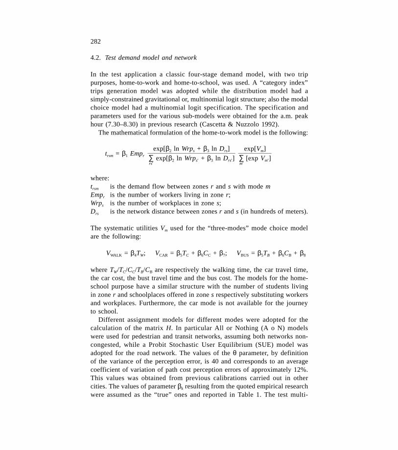
In the test application a classic four-stage demand model, with two trippurposes, home-to-work and home-to-school, was used. A “category index”trips generation model was adopted while the distribution model had asimply-constrained gravitational or, multinomial logit structure; also the modalchoice model had a multinomial logit specification. The specification andparameters used for the various sub-models were obtained for the a.m. peakhour (7.30–8.30) in previous research (Cascetta & Nuzzolo 1992).

The mathematical formulation of the home-to-work model is the following:

where:trsm is the demand flow between zones r and s with mode mEmpr is the number of workers living in zone r;Wrps is the number of workplaces in zone s;Drs is the network distance between zones r and s (in hundreds of meters).

The systematic utilities Vm used for the “three-modes” mode choice modelare the following:

VWALK = β4TW; VCAR = β5TC + β6CC + β7; VBUS = β5TB + β6CB + β8

where TW/TC/CC/TB/CB are respectively the walking time, the car travel time,the car cost, the bust travel time and the bus cost. The models for the home-school purpose have a similar structure with the number of students livingin zone r and schoolplaces offered in zone s respectively substituting workersand workplaces. Furthermore, the car mode is not available for the journeyto school.

Different assignment models for different modes were adopted for thecalculation of the matrix H. In particular All or Nothing (A o N) modelswere used for pedestrian and transit networks, assuming both networks non-congested, while a Probit Stochastic User Equilibrium (SUE) model wasadopted for the road network. The values of the θ parameter, by definitionof the variance of the perception error, is 40 and corresponds to an averagecoefficient of variation of path cost perception errors of approximately 12%.This values was obtained from previous calibrations carried out in othercities. The values of parameter βk resulting from the quoted empirical researchwere assumed as the “true” ones and reported in Table 1. The test multi-

282


trsm = β1 Empr

exp[β2 ln Wrps + β3 ln Drs]

exp[β2 ln Wrps′ + β3 ln Drs′]∑rs′

∑m′

exp[Vm]

[exp Vm′]

modal network has 5 zones (centroids); road and pedestrian networks both havethe same topology with 11 nodes and 36 links. Congestion of the road networkwas simulated through separable cost functions with constant running timesand intersection delays obtained through a simplified Webster formula witha linear extension beyond a flow/capacity ratio of 0.95. The transit networkhas 18 nodes and 48 links with a structure corresponding to two circularlines. The test network is shown in Figure 1. “True” traffic flows were obtainedby assigning to the modal networks the demand obtained through the above-described demand models with “true” parameters.

283


Fig. 1. The test network.

284


Tab

le 1

a.

Res

ults

and

sta

tist

ical

per

form

ance

in

the

test

net

wor

k.

CV

B0.

40.

20.

40.

2C

VF

0.01

0.01

0.4

0.4

Mod

el

Pur

pose

A

ttri

bute

βtrue

β 1*M

SE

%(β

k)β 1*

MS

E%

(βk)

β 1*M

SE

%(β

k)β 1*

MS

E%

(βk)

Gen

er.

H-W

Wor

kers

0.46

0.45

100.

00.

4610

0.0

0.48

72.7

0.45

53.6

Gen

er.

H-S

CS

tude

nts

0.86

0.86

099.

90.

8610

0.0

0.88

66.6

0.88

83.5

Dis

trib

.H

-WD

ista

nces

0.70

0.71

099.

10.

7009

9.6

0.76

44.3

0.71

08.7

Dis

trib

.H

-WW

ork

pl.

1.02

1.03

099.

91.

0309

9.9

0.95

57.9

1.02

33.4

Dis

trib

.H

-SC

Dis

tanc

es0.

930.

8509

7.1

0.92

098.

21.

0365

.50.

9721

.7D

istr

ib.

H-S

CS

choo

l pl

.0.

350.

3609

9.9

0.35

099.

70.

3849

.50.

3509

.3M

od.

ch.

H-W

Wal

king

T.

1.19

1.26

087.

51.

1809

8.3

1.17

80.8

1.26

45.9

Mod

. ch

.H

-WC

ar/B

us T

.0.

540.

4101

2.4

0.52

017.

70.

5303

.90.

5004

.7M

od.

ch.

H-W

Car

/Bus

C.

1.80

1.89

027.

91.

8600

7.9

1.65

00.9

1.87

07.1

Mod

. ch

.H

-W

Car

spe

cif.

2.56

3.06

066.

92.

5407

7.6

2.34

62.4

2.42

51.6

Mod

. ch

.H

-W

Bus

spe

cif.

2.29

2.93

028.

02.

3006

2.2

2.08

18.1

2.30

42.2

Mod

. ch

. H

-SC

Wal

king

T.

2.18

2.55

089.

92.

1709

4.5

2.20

59.3

2.19

72.2

Mod

. ch

.H

-SC

Bus

Tim

e0.

390.

0202

9.6

0.41

035.

70.

4100

.30.

4102

.3M

od.

ch.

H-S

C

Bus

Cos

t1.

582.

3405

9.6

1.56

079.

01.

6739

.91.

5923

.3M

od.

ch.

H-S

C

Bus

spe

cif

1.53

0.96

007.

41.

4700

4.2

1.48

06.0

1.60

06.1

4.3. The evaluation method

Evaluation of the statistical performances of the NGLS estimators (4.1) wascarried out through a Monte-Carlo method by sampling “errors” for initialestimates of the parameters β̂i and for counted flows f̂ 1. In particular, initialestimates β̂i of the parameters were generated by sampling from a normalvariate with a mean equal to the “true” value βtrue and a variance equal to(CVB βtrue)2 where CVB is the variation coefficient assumed for initial estimateerrors. Similarly, counted flows f̂ 1 were generated by sampling from normalvariates with a mean equal to f1 and a coefficient of variation CVF. Bydesigning the simulation test with these characteristics, errors ε and δ wereobtained consistently with the approximation of zero covariance terms in Dand W, the assumption of unbiased errors in β̂ and in f̂ is also respected.

Although the convexity of the objective function (4.1) was not provedanalytically, numerical analyses showed that for the assumed model struc-ture the objective function is strictly convex (Russo & Iannò 1991). Suchanalyses were carried out on several average-sized cities, using the same modelstructure.

In Figure 2 some “sections” of the objective function corresponding toone variable parameter are presented, while keeping all the others fixed tothe “true” values. The diagrams show the correctness of the convexity assump-tion; they also show that for some parameters the objective function is rather“flat” around the optimal values, while for others the slope is rather promi-nent. It can be noted that the incremental ratio of the objective functioncalculated between one extreme of the constant width interval and the middlepoint is about 300 for the generation while about 0.8 for the car/bus costparameter in modal choice.

The “corrected” estimates β* were obtained by imposing only sign constraintson the parameter (e.g. negative costs).

The statistics reported are relative to average values obtained over a set

285


Table 1b. Statistical performances in the test network. Trial set N = 20, links = 40.

CVB 0.4 0.2 0.4 0.2CVF 0.01 0.01 0.4 0.4

Mean MSE%(tn) 099.83 099.97 98.25 95.23Best MSE%(tn) 100 100 99.49 99.04Worst MSE%(tn) 099.04 099.91 96.98 76.04

Mean MSE%( f ) 099.92 099.99 99.27 98.22Best MSE%( f ) 100 100 99.91 99.68Worst MSE%( f ) 099.87 099.98 94.72 89.72

of N trials with the same pair of CVB and CVF values. The following statisticswere defined:

N = total number of trials of a set with the same pair of CVB and CVFvalues

βt = βtrue = vector of true parameters

β̂nin ; β* n = initial and optimal vector of parameters at trial n

286


Fig. 2. Section of the objective function.

OBJnin = value of the objective function in the initial point of trial n

OBJnop = value of the objective function in the optimal point of trial n

RE(OBJn) = [OBJnin – OBJn

op]/OBJnin proportional reduction of the

function in trial n

The Mean Square Error (MSE) statistic was used as an indicator for theestimator’s efficiency (Judge et al. 1988):

MSE(β̂i) = {var(β̂i) + [bias(β̂i)]2}

The following MSE statistics were computed:

MSE%(βk) = [MSE(β̂kin) – MSE(β* k)]/MSE(β̂k

in) proportional reduction of the Mean Square Error in parameter k

In addition to the measure of the deviation of the parameters from the “true”ones, deviations of the demand vector estimated with β* , t(β*) and of theresulting flow vector f = Ht(β*) from true values were computed by usingefficiency indicators similar to those adopted for the parameters. The indica-tors computed for link flows use three vectors: a) flow vector for counted linksflows; b) flow vector for unmeasured links; c) total flow vector.

4.4. Analysis of the results

In numerical tests different levels of error variances were assumed both forflow measurement errors (CVF from 0.01 to 1) and for initial parameterestimates (CVB from 0.20 to 0.60). Two groups of tests were performed withdifferent N; in all cases 40 links were counted corresponding to 30% of all

287


β̂min : β̂in

m, k = β̂inn, k

1N

N

∑n = 1

β* n, kβ* m : β* m, k =1N

N

∑n = 1

mean vector of initial parameters after N trials

mean vector of the optimal parameters afterN trials

1N

N

∑n = 1

1N

N

∑n = 1

MSE(β̂kin) =

MSE(β* k) =

(β̂inn, k – βt

k)2

(β* n, k – βtk)

2

mean square error of initial estimatesof parameter βk

mean square error of final estimatesof parameter βk

network links. The first group was carried out with 20 trials and was aimedat analysing the level of estimates improvements; the second group was per-formed with four trials and aimed at studying the trade-off between computingtime and error reduction.

The “corrected” estimates of parameters are generally very satisfactory.Numerical details of the first group, reported in Table 1a, show the verysmall level of final error for the parameters of generation and distributionmodels.

Modal choice parameters show less satisfactory results. In particular someparameters for home-to-school (H-SC) trips remain with significant MSEvalues, though reduced with respect to initial estimates. Such a result maybe explained by considering that the choice represented by this model is almostconstrained because the students have only two alternative modes (walk-bus),and given the average distance of trips even values of the parameters whichslightly differ from the true ones can reproduce closely the true values oflink flows.

Correction levels for generation and distribution parameters, though veryhigh in all cases, seem to be higher for “work” models than for “school”ones. In general, it can be observed that percentage error reduction (MSE%)is higher for lower measurement and assignment error of counts (CVF) whileno clear indications emerge with respect to starting estimates errors (CVB).

Indicators for the demand vector obtained with the optimal parametersrelative to each trial were also computed. Such indicators give a direct measureof the demand reproduction capability which is one of the main targets ofany demand modelling exercise.

The results reported in Table 1b, show that the percentage reduction of MSEis close to 100% also in the worst case. Obviously, error reductions for demandare smaller for higher counted flow errors (CVF). This result is confirmedby the indicators providing the average of the error reduction in modelleddemand values, after 20 trials of 95% with a worst reduction of 76% (CVB= 0.2; CVF = 0.4) and a best reduction of practically always 100%.

Corresponding indicators for link flows give the same picture, as expected,given the direct derivation of flows from the demand vector by means of theassignment matrix. For all links in all trials, reductions in the initial errorexceeding 90% were obtained.

A second set of four-trial tests was performed in order to analyse the trade-off between computation time and “quality” of estimates.

In general, it was observed (see Table 2) that CVF and CVB exert oppositeinfluences on the two most direct indicators, computation time and averageerror reduction in the parameters. Increasing CVF values, and hence deviationsbetween measured and “true” flows, cause a decrease in the final precisionwhile the calculation time is significantly reduced. On the other hand, an

288


289


Tab

le 2

. I

nflu

ence

of

CV

F a

nd C

VB

on

tim

e an

d re

duct

ion

erro

r. T

rial

set

N=

4,

link

s =

40.

CV

FC

VB

Tim

e co

mpu

tati

on (

h)M

MS

E%

(f)

0.01

0.2

9.96

099.

990.

49.

1610

0.0

0.6

2.11

099.

63

0.2

0.2

2.13

099.

810.

43.

0009

9.72

0.6

3.00

099.

87

0.4

0.2

0.68

098.

220.

41.

6309

9.27

0.6

2.07

096.

11

10.

20.

2308

1.27

0.4

0.93

086.

730.

61.

0309

8.68

increase in CVB produces, with high CVF, an improvement in the parame-ters’ percentage correction, but at the expense of computation time.

Finally trials with the same combinations of CVF and CVB were performedby a 50% reduction in the number of the arcs with measured flow (20) insteadof (40). With respect to the corresponding trials, a substantial reduction incalculation time, was observed: the minimum CPU time (2′) was needed forlarge CVF values (0.4), the maximum CPU time (38′) was needed for smallCVB (0.2) and CVF (0.01) values; high average error reduction (95%) inflow was confirmed. Table 2 also reports the CPU time using a very smallPC with CPU 40286/1MB RAM.

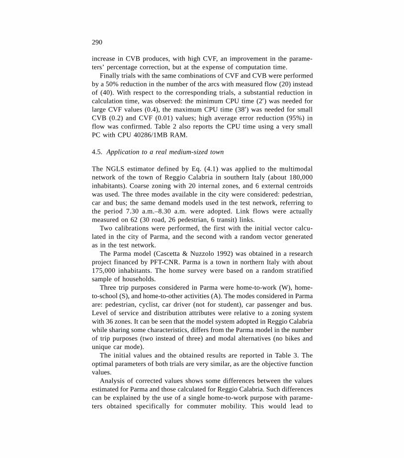
4.5. Application to a real medium-sized town

The NGLS estimator defined by Eq. (4.1) was applied to the multimodalnetwork of the town of Reggio Calabria in southern Italy (about 180,000inhabitants). Coarse zoning with 20 internal zones, and 6 external centroidswas used. The three modes available in the city were considered: pedestrian,car and bus; the same demand models used in the test network, referring tothe period 7.30 a.m.–8.30 a.m. were adopted. Link flows were actuallymeasured on 62 (30 road, 26 pedestrian, 6 transit) links.

Two calibrations were performed, the first with the initial vector calcu-lated in the city of Parma, and the second with a random vector generatedas in the test network.

The Parma model (Cascetta & Nuzzolo 1992) was obtained in a researchproject financed by PFT-CNR. Parma is a town in northern Italy with about175,000 inhabitants. The home survey were based on a random stratifiedsample of households.

Three trip purposes considered in Parma were home-to-work (W), home-to-school (S), and home-to-other activities (A). The modes considered in Parmaare: pedestrian, cyclist, car driver (not for student), car passenger and bus.Level of service and distribution attributes were relative to a zoning systemwith 36 zones. It can be seen that the model system adopted in Reggio Calabriawhile sharing some characteristics, differs from the Parma model in the numberof trip purposes (two instead of three) and modal alternatives (no bikes andunique car mode).

The initial values and the obtained results are reported in Table 3. Theoptimal parameters of both trials are very similar, as are the objective functionvalues.

Analysis of corrected values shows some differences between the valuesestimated for Parma and those calculated for Reggio Calabria. Such differencescan be explained by the use of a single home-to-work purpose with parame-ters obtained specifically for commuter mobility. This would lead to

290


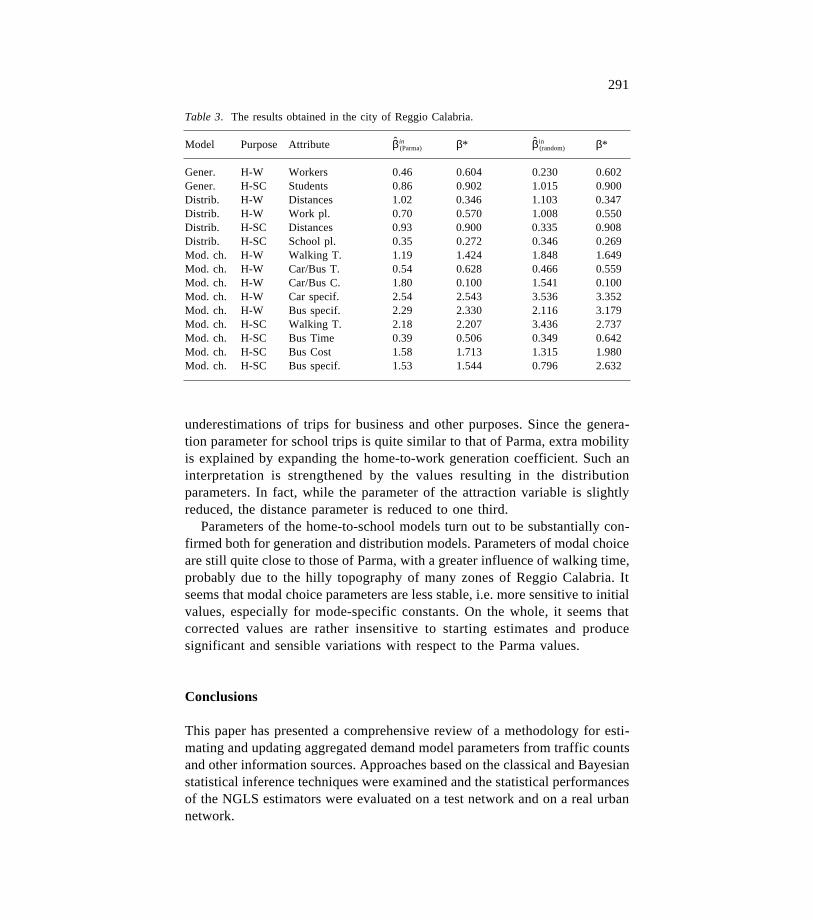
underestimations of trips for business and other purposes. Since the genera-tion parameter for school trips is quite similar to that of Parma, extra mobilityis explained by expanding the home-to-work generation coefficient. Such aninterpretation is strengthened by the values resulting in the distributionparameters. In fact, while the parameter of the attraction variable is slightlyreduced, the distance parameter is reduced to one third.

Parameters of the home-to-school models turn out to be substantially con-firmed both for generation and distribution models. Parameters of modal choiceare still quite close to those of Parma, with a greater influence of walking time,probably due to the hilly topography of many zones of Reggio Calabria. Itseems that modal choice parameters are less stable, i.e. more sensitive to initialvalues, especially for mode-specific constants. On the whole, it seems thatcorrected values are rather insensitive to starting estimates and producesignificant and sensible variations with respect to the Parma values.

Conclusions

This paper has presented a comprehensive review of a methodology for esti-mating and updating aggregated demand model parameters from traffic countsand other information sources. Approaches based on the classical and Bayesianstatistical inference techniques were examined and the statistical performancesof the NGLS estimators were evaluated on a test network and on a real urbannetwork.

291


Table 3. The results obtained in the city of Reggio Calabria.

Model Purpose Attribute β̂in(Parma) β* β̂in

(random) β*

Gener. H-W Workers 0.46 0.604 0.230 0.602Gener. H-SC Students 0.86 0.902 1.015 0.900Distrib. H-W Distances 1.02 0.346 1.103 0.347Distrib. H-W Work pl. 0.70 0.570 1.008 0.550Distrib. H-SC Distances 0.93 0.900 0.335 0.908Distrib. H-SC School pl. 0.35 0.272 0.346 0.269Mod. ch. H-W Walking T. 1.19 1.424 1.848 1.649Mod. ch. H-W Car/Bus T. 0.54 0.628 0.466 0.559Mod. ch. H-W Car/Bus C. 1.80 0.100 1.541 0.100Mod. ch. H-W Car specif. 2.54 2.543 3.536 3.352Mod. ch. H-W Bus specif. 2.29 2.330 2.116 3.179Mod. ch. H-SC Walking T. 2.18 2.207 3.436 2.737Mod. ch. H-SC Bus Time 0.39 0.506 0.349 0.642Mod. ch. H-SC Bus Cost 1.58 1.713 1.315 1.980Mod. ch. H-SC Bus specif. 1.53 1.544 0.796 2.632

The results are in general satisfactory, showing the capability of the proposedestimator to reduce significantly errors in initial estimates. This is particu-larly true for generation and distribution models, while the objective functionis more stable with respect to changes in mode choice parameters. In anycase, modal O/D demand matrices and link flows obtained using correctedparameters virtually coincide with the “true” ones. The application of theestimator to a real network showed its capability to “adapt” to a model mis-specification, modifying generation and distribution parameters to take intoaccount business and other trip purposes initially non-included in the modelbut significant in the real case.

References

Cantarella GE (1996) A General Fixed Point Approach to Multi-mode Multi-user EquilibriumAssignment with Elastic Demand. Internal report. Department of Transportation EngineeringUniversity of Naples.

Cascetta E (1984) Estimation of trip matrices from traffic counts and survey data: A general-ized least squares estimator. Transportation Research 18B: 289–299.

Cascetta E (1986) A Class of Travel Demand Estimators Using Traffic Flows. Publication n.375 CRT Université de Montreal.

Cascetta E (1990) Metodi quantitativi per la pianificazione dei sistemi di trasporto. Padova:Cedam.

Cascetta E & Nguyen S (1988) A unified framework for estimating or updating origin-destina-tion matrices from traffic counts. Transportation Research 22B: 437–455.

Cascetta E & Nuzzolo A (1992) Un modello di equilibrio domanda/offerta per la simulazionedei sistemi di trasporto nelle aree urbane di medie dimensioni. In: Bianco L & Labella A (eds)Strumenti quantitativi per l’analisi dei sistemi di trasporto. Milano: Angeli.

Cascetta E & Russo F (1992) Calibrating travel demand models from traffic counts: statisticalperformances and computational aspect. In: Selected Proceedings of the Sixth WorldConference on Transport Research. Lyon.

Di Gangi M (1989) Una valutazione delle prestazioni statistiche degli estimatori delle matriciO/D che combinano i risultati di indagini e/o modelli con i conteggi di flussi di traffico.Ricerca operativa n. 51: 23–59.

Domencich TA & Mc Fadden D (1975) Urban Travel Demand: A Behavioural Analysis. NewYork: Elsevier.

Judge G, Griffiths W, Lutkepohl H & Lee T (1988) Introduction to the Theory and Practiceof Econometrics. New York: Wyley (2nd Ed.).

Judge G, Griffiths W, Lutkepohl H & Lee T (1988) The Theory and Practice of Econometrics.New York: Wyley.

Hogberg P (1976) Estimation of parameters in models for traffic prediction: a non-linear regres-sion approach. Transportation Research 10B: 263–265.

Lupi M (1989) Conseguenze dell’aleatorietà della matrice di assegnazione sulla stima delladomanda di trasporto mediante conteggi di traffico. Ricerca Operativa n. 51: 61–87.

Maher MJ (1983) Inferences on trip matrices from observations on link volumes: a Bayesianstatistical approach. Transportation Research 17B: 435–447.

Nguyen S. Estimating origin-destination matrices from observed flows. In: Florian M (ed)Transportation Planning Models (pp 363–380). Amsterdam: Elsevier Science Publishers.

292


Nguyen S & Pallottino S (1985) Assegnamento dei passeggeri ad un sistema di Linee Urbane:Determinazione degli Ipercammini Minimi. Ricerca Operativa 38: 29–78.

Russo F & Ianno D (1991) Prestazioni statistiche degli estimatori dei parametri di modelli didomanda con i conteggi di flussi. Quaderno n. 2 della Facoltà di Ingegneria di Reggio Calabria.

Sheffi Y (1985) Urban Transportation Networks. Englewood Cliff: Prentice Hall.Shetty CM & Bazaraa MS (1979) Nonlinear Programming Theory and Algorithms. New York:

Wiley.Spiess H (1983) A Maximum Likelihood Model for Estimating Origin Destination Matrices.

Publication n. 293, CRT Universite de Montreal.Van Zuylen JH & Branston DM (1982) Consistent link flow estimation from counts.

Transportation Research 16B: 473–476.Willumsen LG (1981) Simplified transport models based on traffic count. Transportation 10:

257–278.Willumsen LG & Tamin OZ (1989) Transport demand model estimation from traffic counts.

Transportation 16: 3–26.

293


Calibrating aggregate travel demand models with traffic counts: Estimators and statistical...

Documents

Transcript of Calibrating aggregate travel demand models with traffic counts: Estimators and statistical...