The stabilizing effects of price flexibility in contract-based models

STEVE AMBLER LOUIS PHANEUF

University of Quebec at Montreal

Montreal, Canada

The Stabilizing Efiects of Price Flexibility in Contract-Based Models*

This paper shows that the destabilizing effects of price flexibility due to the increased sensitivity of contract wages to labor market tightness depend on the assumption of a restriction on the information available to wagesetters who are negotiating contract renewals. If these agents are put on the same footing as investors and the monetary authorities by being given access to current information, then increased price flexibility can reduce the magnitude of economic fluctuations in the face of demand shocks. Contrary to other recent papers, this result is derived com- pletely within a staggered contracts framework.

1. Introduction The stabilizing powers of price flexibility have been the object

of a vivid debate. Building on models of the staggered contracts variety, recent papers have offered conflicting views on this matter.

Driskill and Sheffrin (1986) extend Taylor’s (1979, 1980) contract model to include real interest rate effects, and they find that increased price flexibility (in the sense of an increased sensitivity of wages to excess demand in the labor market) can lower the variance of output. De Long and Summers (198613) find that the un- ambiguous stabilizing virtues of price flexibility in Driskill and Shef- frin (1986) h’ g m e on the assumption that only wage shocks can have persistent effects. This is implausible.

De Long and Summers (1986b) address the issue of the stabilizing effects of price flexibility in a model with a richer menu of impulses with long and lasting effects. They find that if demand shocks have persistent effects, then increased price flexibility can actually lead to greater output variability. Their result derives from the Mundell effect: a positive demand shock produces an antici- pated inflation that lowers ex ante real interest rates and leads demand to increase even more. As price flexibility increases, the Mundell effect is strengthened.

*The authors would like to thank (without implicating) Matthew Canzoneri, Stephen King, John Taylor, and an anonymous referee for helpful comments.

Journal of Macroeconomics, Spring 1989, Vol. 11, No. 2, pp. 233-246 233 Copyright 0 1989 by Louisiana State University Press 0164-0704/89/$1.50

Steve Ambler and Louis Phaneuf

We demonstrate that this result depends on the imposition of an arbitrary constraint on the information set available to wagesetters who are negotiating contract renewals. ’ Aside from a backward- looking relative wage effect, the contract decision is affected in the De Long and Summers model only by future expected variables with expectations dated period t - 1, while at the same time the ex ante real interest rate relevant for the determination of aggregate demand is conditioned on an information set dated period t.

There is no theoretical justification for allowing wagesetters whose contracts are up for renegotiation to have access to a limited information set relative to the one that is available to investors and policymakers. Making new wage contracts responsive to the current economic environment guarantees persistent effects of all shocks as in De Long and Summers.2 However, unlike in De Long and Sum- mers, this simultaneous feedback makes current as well as future prices responsive to demand shocks. This weakens the Mundell effect, and price flexibility once again becomes stabilizing for a wide range of parameter values.

This result holds despite the fact that the entire labor force signs multiperiod labor contracts that fix the nominal wage for the duration of the contract (with a fraction of the labor force renego- tiating each period), and despite the existence of a fixed markup pricing rule for firms. Other recent papers (Cantor 1987; Canzoneri and Rogers 1987; Howitt 1986; King 1988) also find circumstances in which price flexibility is stabilizing, but all of the papers except Howitt (1986) use models in which at least part of the labor force have their wages determined in a spot market (King,’ Cantor), or in which contracts are negotiated according to an expected market- clearing rule with both the possibility of wage indexation on current price level changes3 and flexible prices in the goods market (Can- zoneri and Rogers).4 In contrast to these other papers, this paper

‘This problem is not specific to De Long and Summers (198613) but to staggered contracts models in general.

‘Driskill and She&n (1986) consider a variation of their model in which current wage contracts respond to current labor market conditions, but they do not seek to provide underpinnings for their assumption and they consider only wage shocks as a source of business cvcle fluctuations.

3Given the empirical unimportance of wage indexation, at least in the American economy, we consider this route to be an unsatisfactory way of restoring the stabilizing effects of price flexibility.

4Howitt (1986) uses a model in which wages respond to unemployment with a lag in order to obtain similar results to De Long and Summers (1986b). However, he notes (without demonstrating formally) that

234

Stabilizing Effects of Price Flexibility

establishes that price flexibility can be stabilizing while remaining entirely within the staggered contracts framework.

The second section describes the modified version of the overlapping contracts model. Section 3 presents the results of numerical simulations indicating that price flexibility is generally stabilizing and that a forward-looking bias in the wage-setting process makes price flexibility even more strongly stabilizing. Section 4 contains con- cluding remarks.

2. The Model The model can be described by the following equations:

y, = m, - p, + y i, (LM curve) , (1)

yt = -0~ [it - (QQ+I - Al + 72, (1s curve) , (2)

7tt = t.~ 7~~~~ + E, (demand shock process) , (3)

m, = pit (money supply rule) , (4)

p, = 0.5 (w, + wt-J (price level definition) , (5)

wt = P b-1 + m) + (1 - P)@w~+I + gEtyt+d

+ qt (wage-setting equation) ; (6)

where all variables except interest rates are measured in logarithms, and where

y = real output, m = the nominal money stock, p = the aggregate price level,

The results depend heavily on the assumption that the effect on wages of an increase in employment works with a one-period delay. Without this delay the multiplier process resulting from Keynes’ expectations effect would not arise, because an increase in demand would have an immediate effect on wages, which would start to go away in the following period. Thus it would give rise to the expectation of deflation, not inflation, an expectation that would dampen the impact on employment rather than amplify it.

235


w = the contract wage, i = the nominal interest rate,

q = a serially uncorrelated shock to the current contract wage, rr = a serially correlated demand shift term, and E = a serially uncorrelated innovation in the demand shift pro-

cess.

The aggregate demand sector (Equations [l] through [4]) of the model is standard. Following Driskill and Sheffrin (1986) and De Long and Summers (1986b), we allow aggregate demand to be sensitive to real interest rates, in contrast to Taylor’s (1979, 1980) original staggered-contracts model in which demand is determined by a quantity theory equation.

Equations (5) and (6) constitute the wage and price determination sector of the model. It is assumed for simplicity that there are two equal groups of workers, each of which negotiates a two- period contract so that wage negotiations reopen for one of the two groups each period. Equation (5) states that prices are determined as a fixed markup over wage costs.

Equation (6) describes the wage determination process in the economy. Wages are &ected by the emulation of the other group’s current wage and expected future wage, and by current and expected labor market tightness. The formulation is standard in the staggered contracts literature except for two crucial modifications. First, the contract wage is now sensitive to the economic conditions observed during the period that negotiations take place as well as to future economic conditions expected to prevail over the course of the contract. This has the immediate implication that expectations are now dated period t so that wagesetters who are negotiating new contracts are on the same footing as investors and policymakers when forming expectations. 5

This amendment to the wage equation gives a more realistic representation of the way the wage negotiation process actually works. In a discrete time model, the current contract wage is an aggregate of many individual wage contracts that are signed over the course of the period in the same way that ilow variables, such as con-

5The possibility of a feedback of this type has been recognized by Taylor (1980, 5; 1981, 74). However, it is only recently that it has been implemented in the staggered wage models of Carlozzi and Taylor (1985) and Driskill and Sheffrin (1986) without an analysis of its implications for the persistence of aggregate demand shocks on output fluctuations.

236


sumption, are an aggregate of flows throughout the period. If current consumption depends to some extent on the current economic environment, then so will the current wage contract.

The second modification to the wage equation, (6), is the introduction of the p parameter, which indicates the relative importance attached by contracting parties to the use of known information (past and current) in making contracts. The terms associated with (1 - p) represent the relative importance attached to expected future developments.

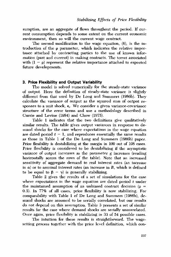
3. Price Flexibility and Output Variability The model is solved numerically for the steady-state variance

of output. Here the definition of steady-state variance is slightly different from that used by De Long and Summers (1986b). They calculate the variance of output as the squared sum of output re- sponses to a unit shock, E,. We consider a given variance-covariance structure of the error terms and use a methodology described in Currie and Levine (1984) and Chow (1975).

Table 1 indicates that the two definitions give qualitatively similar results. The table gives output variances in response to demand shocks for the case where expectations in the wage equation are dated period t - 1, and reproduces essentially the same results as those in Table 1 of the De Long and Summers (1986b) paper. Price flexibility is destabilizing at the margin in 100 out of 108 cases. Price flexibility is considered to be destabilizing if the asymptotic variance of output increases as the parameter g increases (reading horizontally across the rows of the table). Note that an increased sensitivity of aggregate demand to real interest rates (an increase in CX) or to nominal interest rates (an increase in B, which is defined to be equal to p - y) is generally stabilizing.

Table 2 gives the results of a set of simulations for the case where expectations in the wage equation are dated period t under the maintained assumption of an unbiased contract decision (p = 0.5). In 77% of all cases, price flexibility is now stabilizing. For comparability with Table 1 of De Long and Summers (1986b), demand shocks are assumed to be serially correlated, but our results do not depend on this assumption. Table 3 presents a set of similar results for the case where demand shocks are serially uncorrelated. Once again, price flexibility is stabilizing in 33 of 54 possible cases.

The intuition for these results is straightforward. The wagesetting process together with the price level definition, which con-

237

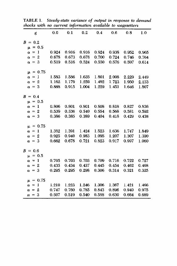
TABLE 1. Steady-state variance of output in response to demand shocks with no current information available to wagesetters

g 0.0 0.1 0.2 0.4 0.6 0.8 1.0

B = 0.2 p = 0.5 a=1 0.924 0.916 0.916 0.924 0.938 0.952 0.965 a=2 0.678 0.673 0.678 0.700 0.724 0.746 0.764 a=3 0.519 0.516 0.524 0.550 0.576 0.597 0.614

/J, = 0.75 a=1 1.583 1.586 1.635 1.801 2.008 2.229 2.449 a=2 1.162 1.179 1.259 1.482 1.723 1.950 2.153 a=3 0.888 0.915 1.004 1.229 1.451 1.646 1.807

B = 0.4 /J, = 0.5 a=1 0.806 0.801 0.801 0.808 0.818 0.827 0.836 a=2 0.539 0.536 0.540 0.554 0.568 0.581 0.592 a=3 0.386 0.385 0.389 0.404 0.418 0.429 0.438

p = 0.75 a=1 1.382 1.391 1.424 1.523 1.636 1.747 1.849 a=2 0.925 0.940 0.983 1.095 1.207 1.307 1.390 a=3 0.662 0.678 0.721 0.823 0.917 0.997 1.060

B = 0.6 p = 0.5 a=1 0.705 0.703 0.703 0.709 0.716 0.722 0.727 a=2 0.435 0.434 0.437 0.445 0.454 0.462 0.468 a=3 0.295 0.295 0.298 0.306 0.314 0.321 0.325

p = 0.75 a=1 1.210 1.223 1.246 1.306 1.367 1.421 1.466 a=2 0.747 0.760 0.785 0.843 0.896 0.940 0.975 a=3 0.507 0.519 0.540 0.588 0.630 0.664 0.689

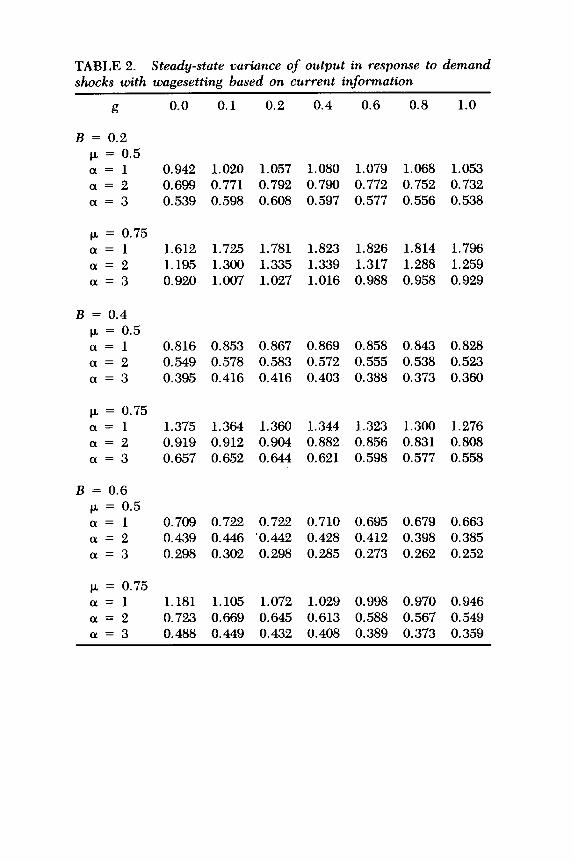
TABLE 2. Steady-state variance of output in response to demand shocks with wagesetting based on current information

g 0.0 0.1 0.2 0.4 0.6 0.8 1.0

B = 0.2 f.k = 0.5 a=1 0.942 1.020 1.057 1.080 1.079 1.068 1.053 a=2 0.699 0.771 0.792 0.790 0.772 0.752 0.732 a=3 0.539 0.598 0.608 0.597 0.577 0.556 0.538

p = 0.75 a=1 1.612 1.725 1.781 1.823 1.826 1.814 1.796 a=2 1.195 1.300 1.335 1.339 1.317 1.288 1.259 a=3 0.920 1.007 1.027 1.016 0.988 0.958 0.929

B = 0.4 p = 0.5 a=1 0.816 0.853 0.867 0.869 0.858 0.843 0.828 a=2 0.549 0.578 0.583 0.572 0.555 0.538 0.523 a=3 0.395 0.416 0.416 0.403 0.388 0.373 0.360

p, = 0.75 a=1 1.375 1.364 1.360 1.344 1.323 1.300 1.276 a=2 0.919 0.912 0.904 0.882 0.856 0.831 0.808 a=3 0.657 0.652 0.644 0.621 0.598 0.577 0.558

B = 0.6 p = 0.5 a=1 0.709 0.722 0.722 0.710 0.695 0.679 0.663 a=2 0.439 0.446 '0.442 0.428 0.412 0.398 0.385 a=3 0.298 0.302 0.298 0.285 0.273 0.262 0.252

p = 0.75 a=1 1.181 1.105 1.072 1.029 0.998 0.970 0.946 a=2 0.723 0.669 0.645 0.613 0.588 0.567 0.549 a=3 0.488 0.449 0.432 0.408 0.389 0.373 0.359


TABLE 3. Steady-state variance of output in response to demand shocks with wagesetting based on current information and uncorrelated demand shocks

g

B = 0.2 p=o a=1 a=2 a=3

B = 0.4 p=o Cl=1 (Y=2 01=3

B = 0.6 p=o a=1 a=2 cX=3

0.0 0.1 0.2 0.4 0.6 0.8 1.0

0.698 0.722 0.736 0.746 0.746 0.742 0.735 0.515 0.538 0.547 0.547 0.539 0.529 0.518 0.395 0.415 0.420 0.415 0.405 0.394 0.384

0.608 0.623 0.631 0.636 0.634 0.628 0.621 0.408 0.421 0.425 0.423 0.416 0.408 0.399 0.293 0.303 0.305 0.301 0.293 0.285 0.278

0.531 0.541 0.545 0.546 0.542 0.536 0.529 0.328 0.336 0.337 0.334 0.328 0.321 0.314 0.223 0.228 0.229 0.225 0.219 0.213 0.208

stitutes the supply side of the overlapping contracts model, can be solved to yield the following aggregate price line:6

pt = oagyt + 0.5(1 - P)&Y,,l + 0.5(1 + Phi

+ 0.5(1 - (l)E,W,,l . (7)

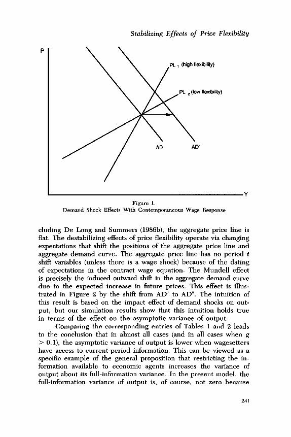
As the price flexibility parameter, g, increases, the price line becomes steeper. The other equations of the model can be used to derive an aggregate demand curve. For a given demand shock, which shifts the aggregate demand curve horizontally, the impact effect on output is weaker the steeper the aggregate price line is. This effect is illustrated in Figure 1, with the aggregate demand curve shifting horizontally from AD to AD’.

In most of the literature on staggered contract models, in-

%ince expectations of future variables are not solved, the position of the price line should be interpreted as being conditional on given expectations.

240


pi , (high flexibility)

Figure 1. Demand Shock Effects With Contemporaneous Wage Response

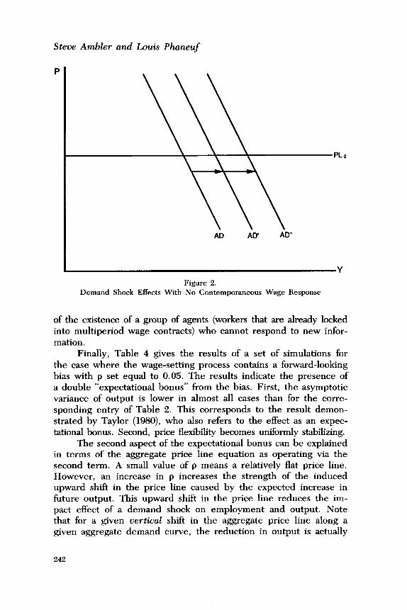
eluding De Long and Summers (1986b), the aggregate price line is flat. The destabilizing effects of price flexibility operate via changing expectations that shift the positions of the aggregate price line and aggregate demand curve. The aggregate price line has no period t shift variables (unless there is a wage shock) because of the dating of expectations in the contract wage equation. The Mundell effect is precisely the induced outward shift in the aggregate demand curve due to the expected increase in future prices. This effect is illustrated in Figure 2 by the shift from AD’ to AD”. The intuition of this result is based on the impact effect of demand shocks on output, but our simulation results show that this intuition holds true in terms of the effect on the asymptotic variance of output.

Comparing the corresponding entries of Tables 1 and 2 leads to the conclusion that in almost all cases (and in all cases when g > 0. l), the asymptotic variance of output is lower when wagesetters have access to current-period information. This can be viewed as a specific example of the general proposition that restricting the information available to economic agents increases the variance of output about its full-information variance. In the present model, the full-information variance of output is, of course, not zero because

241


PLO

AD AD’ AD”

Figure 2. Demand Shock Effects With No Contemporaneous Wage Response

of the existence of a group of agents (workers that are already locked into multiperiod wage contracts) who cannot respond to new information.

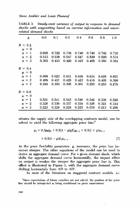
Finally, Table 4 gives the results of a set of simulations for the case where the wage-setting process contains a forward-looking bias with p set equal to 0.05. The results indicate the presence of a double “expectational bonus” from the bias. First, the asymptotic variance of output is lower in almost all cases than for the corresponding entry of Table 2. This corresponds to the result demon- strated by Taylor (1980), who also refers to the effect as an expectational bonus. Second, price flexibility becomes uniformly stabilizing.

The second aspect of the expectational bonus can be explained in terms of the aggregate price line equation as operating via the second term. A small value of p means a relatively flat price line. However, an increase in p increases the strength of the induced upward shift in the price line caused by the expected increase in future output. This upward shift in the price line reduces the impact effect of a demand shock on employment and output. Note that for a given vertical shift in the aggregate price line along a given aggregate demand curve, the reduction in output is actually

242

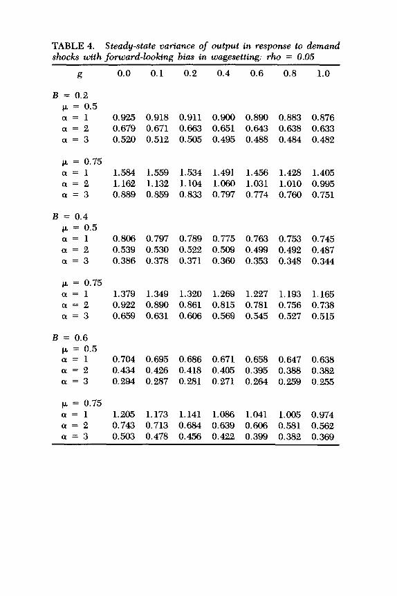
TABLE 4. Steady-state variance of output in response to demand shocks with forward-looking bias in wagesetting: r-ho = 0.05

g 0.0 0.1 0.2 0.4 0.6 0.8 1.0

B = 0.2 p, = 0.5 a=1 0.925 0.918 0.911 0.900 0.890 0.883 0.876 a=2 0.679 0.671 0.663 0.651 0.643 0.638 0.633 a=3 0.520 0.512 0.505 0.495 0.488 0.484 0.482

k = 0.75 a=1 1.584 1.559 1.534 1.491 1.456 1.428 1.405 a=2 1.162 1.132 1.104 1.060 1.031 1.010 0.995 a=3 0.889 0.859 0.833 0.797 0.774 0.760 0.751

B = 0.4 p = 0.5 a=1 0.806 0.797 0.789 0.775 0.763 0.753 0.745 a=2 0.539 0.530 0.522 0.509 0.499 0.492 0.487 a=3 0.386 0.378 0.371 0.360 0.353 0.348 0.344

k = 0.75 a=1 1.379 1.349 1.320 1.269 1.227 1.193 1.165 a=2 0.922 0.890 0.861 0.815 0.781 0.756 0.738 a=3 0.659 0.631 0.606 0.569 0.545 0.527 0.515

B = 0.6 c* = 0.5 a=1 0.704 0.695 0.686 0.671 0.658 0.647 0.638 a=2 0.434 0.426 0.418 0.405 0.395 0.388 0.382 a=3 0.294 0.287 0.281 0.271 0.264 0.259 0,255

p, = 0.75 a=1 1.205 1.173 1.141 1.086 1.041 1.005 0,974 a=2 0.743 0.713 0.684 0.639 0.606 0.581 0.562 a=3 0.503 0.478 0.456 0.422 0.399 0.382 0.369


greater if the price line is flat than if it is steep. Increasing the size of the vertical shift also has more of a stabilizing effect.

In the version of the model without access to current-period information by wagesetters, there is still an expectational bonus that reduces the variance of output in response to wage shocks. How- ever, since the price line is horizontal and contains no period t shift variables, both aspects of the expectational bonus are inoperative in response to serially uncorrelated demand shocks. Demand shocks affect aggregate demand and hence output in the period in which they occur, but they have no persistence. The asymptotic variance of output depends on none of the structural parameters that enter the price line equation.7

The above results leave the stylized fact of the increasing de- gree of nominal rigidity in the U.S. economy over the past century combined with an apparent decrease in the magnitude of output fluctuations (compare De Long and Summers 1986a, 198613; King 1988) still to be explained. Ambler and Phaneuf (1987) demonstrate, using a model similar to the one in the present paper, that when monetary policy partially accommodates price level changes (which many would also contend to have been a stylized fact of monetary policy in the U.S. and other economies), an inverse trade-off between price level and output variability (Taylor’s [1979, 19801 so- called second-order Phillips curve) disappears when demand shocks dominate. An inappropriate response of monetary policy to demand shocks, combined with a contemporaneous response of wages and prices to labor market conditions, is capable of explaining the observed stylized facts of the American business cycle.

4. Conclusions This paper demonstrates that the positive relationship be-

tween price flexibility and the cyclical variability of output in Keynesian models depends on a restriction being placed on the information available to wagesetters. If it is realistic to allow wagesetters to use the same information set as investors when they ne- gotiate contract renewals, then price flexibility generally becomes more stabilizing even if the entire labor force binds its hands by signing multiperiod contracts that fix the nominal wage for the du-

‘When demand shocks are serially correlated, the possibility of an expectational

bonus once again reappears.

244


ration of the contract. It is clear that this conclusion continues to hold for the scenarios considered by De Long and Summers (198613) for which price flexibility can be stabilizing, such as when supply shocks dominate or when aggregate demand is determined by Tobin’s q.

Received: January 1988 Final version: June 1988

References Ambler, S., and L. Phaneuf. “Accommodation and Fluctuations.”

Working paper, University of Quebec at Montreal, Canada, March 1987.

Cantor, R. “Increased Price Flexibility and Aggregate Output Sta- bility: A Note.” Working paper, University of California at Los Angeles, January 1987.

Canzoneri, M.B., and C.A. Rogers. “Is Increased Prjce Flexibility Stabilizing? Comment.” Working paper, Georgetown University, Washington, D.C., May 1987.

Carlozzi, N., and J.B. Taylor. “International Capital Mobility and the Coordination of Monetary Rules.” Exchange Rate Manage- ment Under Uncertainty, edited by J. Bhandari, 186-211. Cam- bridge, MA: MIT Press, 1985.

Chow, G.C. Analysis and Control of Dynamic Economic Systems. New York, NY: John Wiley, 1975.

Currie, D., and P. Levine. “Stochastic Macroeconomic Policy Sim- ulations for a Small Open Economy.” Mathematical Methods in Economics, edited by F. van der Ploeg, 217-48. New York, NY: John Wiley, 1984.

De Long, B., and L. Summers. “The Changing Cyclical Variability of Economic Activity in the United States.” The American Busi- ness Cycle: Continuity and Change, edited by R. J. Gordon. Chi- cago, IL: University of Chicago Press, 1986a.

-. “Is Increased Price Flexibility Stabilizing?” American Eco- nomic Review 76 (December 1986b): 1031-44.

Driskill, R., and S. ShefIi-in. “Is Price Flexibility Destabilizing?” American Economic Review 76 (September 1986): 802-7.

Howitt, P. “Wage Flexibility and Employment.” Eastern Journal of Economics 12 (July-September 1986): 237-42.

King, S.R. “Is Increased Price Flexibility Stabilizing: A Comment.” American Economic Review 78 (March 1988): 267-72.

245


Taylor, J.B. “Staggered Wage Setting in a Macro Model.” American Economic Review 69 (May 1979): 198-13.

-. “Aggregate Dynamics and Staggered Contracts.” Journal of Political Economy 88 (February 1980): l-23.

-. “On the Relation Between the Variability of Inflation and the Average Inflation Rate.” In The Costs and Consequences of Inflation, edited by K. Brunner and A.H. Meltzer, 57-86. Car- negie Rochester Conference Series on Public Policy, 15. Am- sterdam: North-Holland, 1981.

246

The stabilizing effects of price flexibility in contract-based models

Documents

Transcript of The stabilizing effects of price flexibility in contract-based models