Parametrization and Effectiveness of Moving Target Defense ...
205
Parametrization and Effectiveness of Moving Target Defense Security Protections within Industrial Control Systems By Adrian R Chavez B.S. University of New Mexico 2004 M.S. University of Colorado at Boulder 2005 Dissertation Submitted in partial satisfaction of the requirements for the degree of Doctor of Philosophy in COMPUTER SCIENCE in the Office of Graduate Studies of the University of California Davis Approved: Dr. Sean Peisert, Chair Dr. Matthew Bishop Dr. Karl Levitt Committee in Charge 2017 -i-
-
Upload
khangminh22 -
Category
Documents
-
view
1 -
download
0
Transcript of Parametrization and Effectiveness of Moving Target Defense ...

Parametrization and Effectiveness of Moving Target Defense SecurityProtections within Industrial Control Systems
By
Adrian R ChavezB.S. University of New Mexico 2004
M.S. University of Colorado at Boulder 2005
Dissertation
Submitted in partial satisfaction of the requirements for the degree of
Doctor of Philosophy
in
COMPUTER SCIENCE
in the
Office of Graduate Studies
of the
University of California
Davis
Approved:
Dr. Sean Peisert, Chair
Dr. Matthew Bishop
Dr. Karl Levitt
Committee in Charge
2017
-i-

Copyright c© 2017 by
Adrian R Chavez
All rights reserved.

To Natasha Garcia, Penelope Chavez, Miles Chavez and all of my family.
-ii-

Contents
List of Figures . . . . . . . . . . . . . . . . . . . . . . . . . . . . . . . . . . . . vii
Abstract . . . . . . . . . . . . . . . . . . . . . . . . . . . . . . . . . . . . . . . xvi
Acknowledgments . . . . . . . . . . . . . . . . . . . . . . . . . . . . . . . . . . xvii
1 Introduction 1
1.1 Challenges . . . . . . . . . . . . . . . . . . . . . . . . . . . . . . . . . . . 3
1.2 Contributions . . . . . . . . . . . . . . . . . . . . . . . . . . . . . . . . . 4
1.2.1 MTD within Critical Infrastructure . . . . . . . . . . . . . . . . . 5
1.2.2 Operational System Impacts . . . . . . . . . . . . . . . . . . . . . 7
1.2.3 Adversary Workload Impacts . . . . . . . . . . . . . . . . . . . . 8
1.3 Organization . . . . . . . . . . . . . . . . . . . . . . . . . . . . . . . . . 9
2 Background 10
2.1 Moving Target Defense Techniques . . . . . . . . . . . . . . . . . . . . . 13
2.2 MTD Categories . . . . . . . . . . . . . . . . . . . . . . . . . . . . . . . 14
2.2.1 Dynamic Platforms . . . . . . . . . . . . . . . . . . . . . . . . . . 14
2.2.2 Dynamic Runtime Environments . . . . . . . . . . . . . . . . . . 15
2.2.3 Dynamic Networks . . . . . . . . . . . . . . . . . . . . . . . . . . 16
2.2.4 Dynamic Data . . . . . . . . . . . . . . . . . . . . . . . . . . . . . 17
2.2.5 Dynamic Software . . . . . . . . . . . . . . . . . . . . . . . . . . 18
2.3 Research Goals . . . . . . . . . . . . . . . . . . . . . . . . . . . . . . . . 21
3 MTD Applications and Scenarios 25
3.1 Industrial Control Systems . . . . . . . . . . . . . . . . . . . . . . . . . . 26
3.1.1 Use Case . . . . . . . . . . . . . . . . . . . . . . . . . . . . . . . . 27
3.1.2 Constraints . . . . . . . . . . . . . . . . . . . . . . . . . . . . . . 29
3.1.3 Requirements . . . . . . . . . . . . . . . . . . . . . . . . . . . . . 30
3.2 Information Technology Systems . . . . . . . . . . . . . . . . . . . . . . . 31
3.2.1 Use Case . . . . . . . . . . . . . . . . . . . . . . . . . . . . . . . . 33
-iii-

3.2.2 Constraints . . . . . . . . . . . . . . . . . . . . . . . . . . . . . . 33
3.2.3 Requirements . . . . . . . . . . . . . . . . . . . . . . . . . . . . . 34
3.3 Cloud Computing Systems . . . . . . . . . . . . . . . . . . . . . . . . . . 35
3.3.1 Use Case . . . . . . . . . . . . . . . . . . . . . . . . . . . . . . . . 36
3.3.2 Constraints . . . . . . . . . . . . . . . . . . . . . . . . . . . . . . 37
3.3.3 Requirements . . . . . . . . . . . . . . . . . . . . . . . . . . . . . 38
4 Threat Model 40
4.1 Operational Impacts . . . . . . . . . . . . . . . . . . . . . . . . . . . . . 43
4.2 Adversarial Models . . . . . . . . . . . . . . . . . . . . . . . . . . . . . . 44
5 Implementation Details 45
5.1 IP Randomization . . . . . . . . . . . . . . . . . . . . . . . . . . . . . . . 46
5.2 Port Randomization . . . . . . . . . . . . . . . . . . . . . . . . . . . . . 50
5.3 Path Randomization . . . . . . . . . . . . . . . . . . . . . . . . . . . . . 52
6 Fault Tolerance Theory 56
6.1 Crash Tolerant Algorithms . . . . . . . . . . . . . . . . . . . . . . . . . . 57
6.1.1 Two-phase Commit . . . . . . . . . . . . . . . . . . . . . . . . . . 59
6.1.2 Three-phase Commit . . . . . . . . . . . . . . . . . . . . . . . . . 61
6.1.3 Replication - Paxos . . . . . . . . . . . . . . . . . . . . . . . . . . 64
6.2 Byzantine Fault Tolerant Algorithms . . . . . . . . . . . . . . . . . . . . 67
6.3 Adversarial Models . . . . . . . . . . . . . . . . . . . . . . . . . . . . . . 69
6.4 Operational Impacts . . . . . . . . . . . . . . . . . . . . . . . . . . . . . 71
7 Overview of Experimental Setups 73
8 Simulation Environments 77
8.1 Adversary Guessing Strategies . . . . . . . . . . . . . . . . . . . . . . . . 78
8.1.1 Serial Guessing . . . . . . . . . . . . . . . . . . . . . . . . . . . . 78
8.1.2 Random Start, Serial Guessing . . . . . . . . . . . . . . . . . . . 82
8.1.3 Random Guessing with Repetition . . . . . . . . . . . . . . . . . 83
-iv-

8.1.4 Random Guessing without Repetition . . . . . . . . . . . . . . . . 85
8.2 Summary . . . . . . . . . . . . . . . . . . . . . . . . . . . . . . . . . . . 86
9 Virtualization Environments 88
9.1 Application Port Randomization Overhead Cost . . . . . . . . . . . . . . 90
9.2 IP Randomization Overhead Costs . . . . . . . . . . . . . . . . . . . . . 91
9.3 Path Randomization Overhead Cost . . . . . . . . . . . . . . . . . . . . . 98
9.4 Port, IP and Path randomization . . . . . . . . . . . . . . . . . . . . . . 100
9.5 Summary . . . . . . . . . . . . . . . . . . . . . . . . . . . . . . . . . . . 102
10 Representative Environments 104
10.1 DETERLab Testbed . . . . . . . . . . . . . . . . . . . . . . . . . . . . . 104
10.1.1 Software Defined Networking . . . . . . . . . . . . . . . . . . . . 108
10.1.2 Threat Model . . . . . . . . . . . . . . . . . . . . . . . . . . . . . 109
10.1.3 Adversary Evaluation . . . . . . . . . . . . . . . . . . . . . . . . . 110
10.1.4 Results . . . . . . . . . . . . . . . . . . . . . . . . . . . . . . . . . 113
10.1.5 Analysis . . . . . . . . . . . . . . . . . . . . . . . . . . . . . . . . 115
10.1.6 Binomial Distribution . . . . . . . . . . . . . . . . . . . . . . . . 115
10.1.7 Hypergeometric Distribution . . . . . . . . . . . . . . . . . . . . . 117
10.2 Virtual Power Plant . . . . . . . . . . . . . . . . . . . . . . . . . . . . . 122
10.2.1 Metrics . . . . . . . . . . . . . . . . . . . . . . . . . . . . . . . . 125
10.2.2 IPv4 . . . . . . . . . . . . . . . . . . . . . . . . . . . . . . . . . . 126
10.2.3 Operational Impacts . . . . . . . . . . . . . . . . . . . . . . . . . 126
10.2.4 Fault Tolerance . . . . . . . . . . . . . . . . . . . . . . . . . . . . 134
10.2.5 IPv6 . . . . . . . . . . . . . . . . . . . . . . . . . . . . . . . . . . 151
10.2.6 Individual Adversaries . . . . . . . . . . . . . . . . . . . . . . . . 152
10.2.7 Distributed Adversaries . . . . . . . . . . . . . . . . . . . . . . . 155
10.2.8 Side Channel Attacks . . . . . . . . . . . . . . . . . . . . . . . . . 158
11 Conclusions 161
11.1 Limitations and Lessons Learned . . . . . . . . . . . . . . . . . . . . . . 161
-v-

11.2 Future Work . . . . . . . . . . . . . . . . . . . . . . . . . . . . . . . . . . 164
11.3 Summary . . . . . . . . . . . . . . . . . . . . . . . . . . . . . . . . . . . 166
-vi-

List of Figures
3.1 An example power grid that shows the high level components from gen-
eration of power to transmission to distribution and finally to delivery at
a residential home. . . . . . . . . . . . . . . . . . . . . . . . . . . . . . . 27
3.2 An example enterprise network with the core layer supporting the back-
bone of the network, the distribution layer supporting communications
within the enterprise, and the access layer connecting end users and
servers. The diagram here shows two departments (A and B) with access
to web, email, and human resources servers. These networks also typically
have an Internet connection through a demilitarized zone to protect the
network with firewall, proxy and security services from external threats. 32
3.3 An example of several users accessing cloud computing resources such as
IaaS, SaaS, and PaaS services. . . . . . . . . . . . . . . . . . . . . . . . 35
5.1 The sequence of events that cause packets to be dropped when random-
izing source and destination IP addresses within an SDN setting. . . . . 49
5.2 The sequence of events to correct dropped packets from occurring when
randomizing source and destination IP addresses within an SDN setting. 51
5.3 An example of two hosts communicating through random paths taken as
shown in the red circled text in the command prompt window. The first
path taken is h1→s1→s2→s3→s4→h2, while the next random path taken
is h1→s1→s4→h2 . . . . . . . . . . . . . . . . . . . . . . . . . . . . . . 55
6.1 The two-phase commit protocol between a coordinator system and a clus-
ter of SDN controllers. The goal is to detect and withstand faults within
the SDN controllers and to synchronize internal state information when
transactions are executed on all controllers. . . . . . . . . . . . . . . . . 60
-vii-

6.2 The three-phase commit protocol between a coordinator system and a
cluster of SDN controllers. The goal is to detect and withstand faults
within the SDN controllers and to synchronize internal state information
when transactions are executed on all controllers. An additional state,
pre-prepare, is added to reduce the amount of time blocking when the
coordinator is waiting on controller responses. . . . . . . . . . . . . . . . 63
8.1 The probability of correctly discovering a randomly-selected 16-bit port
number using different guessing strategies given a limited number of probes. 79
8.2 The average number of attempts expected before correctly discovering a
randomly-selected 16-bit port number using different guessing strategies
where the adversary is given a limited number of probes. . . . . . . . . . 80
8.3 The average amount of time needed before correctly discovering a randomly-
selected 16-bit port number using different guessing strategies where the
adversary is given a limited number of probes. . . . . . . . . . . . . . . . 81
9.1 A diagram of an example network where host A wishes to communicate
with host B. The OpenDaylight controller inserts flows within the overlay
network so that packets have randomized source and destination IP ad-
dresses, randomized port numbers, and take random paths (shown as the
red and green lines through overlay network) through the network. . . . 89
9.2 The RTT measured across 10,000 pings with port randomization disabled
and enabled. . . . . . . . . . . . . . . . . . . . . . . . . . . . . . . . . . 90
9.3 The bandwidth measured across a 10,000 second (∼2.77 hours) period of
time when application port number randomization is disabled and enabled. 91
9.4 The RTT measured across 10,000 pings when IP randomization is disabled
and enabled. . . . . . . . . . . . . . . . . . . . . . . . . . . . . . . . . . 92
9.5 The average bandwidth measured over a 10,000 second (∼2.77 hours)
period when IP randomization is disabled and enabled. . . . . . . . . . . 93
-viii-

9.6 The average throughput measured over a 10,000 second (∼2.77 hours)
period of time when IP randomization is disabled and enabled. . . . . . 94
9.7 The average bandwidth measured over a 10,000 second (∼2.77 hours)
period when IP randomization is disabled and enabled. . . . . . . . . . . 95
9.8 The probability of correctly discovering a randomly-selected 24-bit num-
ber (a CIDR class A IP Address) using different guessing strategies given
a limited number of probes. . . . . . . . . . . . . . . . . . . . . . . . . . 96
9.9 The expected number of attempts to randomly find a 24-bit number (a
CIDR class A IP Address) using different guessing strategies given a lim-
ited number of probes. . . . . . . . . . . . . . . . . . . . . . . . . . . . . 98
9.10 Performance metrics of a normal network without randomization tech-
niques introduced, with the three randomization algorithms implemented
independently, and finally with all three algorithms combined and applied. 99
9.11 Performance metrics when transferring 1 MB files within the Tor network
over a three-month period of time. . . . . . . . . . . . . . . . . . . . . . 102
10.1 An experiment allocated within the DETERLab testbed consisting of 16
adversarial nodes labeled nodeE1-nodeE16 and 4 operational nodes la-
beled nodeA-nodeD. . . . . . . . . . . . . . . . . . . . . . . . . . . . . . 107
10.2 The solid lines represent the number of attempted spoofed packets that
need to be injected into the network with varying frequencies of re-randomizing
IP addresses. As the randomization frequencies increase in time, the num-
ber of required attempted adversary spoofed packets before a successful
packet is injected decreases. The dashed lines represent the theoretical
expectation results of the binomial distribution, which match the exper-
imented data closely. Each of the curves represents the total number of
adversaries, varying from 1 adversary to 65,536 adversaries. The frequency
intervals vary from 0.5 seconds to a static configuration. We performed
10,000 trials with an adversary that was capable of injecting 310 packets
per second in the test environment provided. . . . . . . . . . . . . . . . 116
-ix-
10.3 The hypergeometric distribution is followed when the adversary randomly
spoofs the source and destination IP addresses until a success occurs with-
out repeating previous failed attempts. The results captured experimen-
tally match those of the expectation curve when varying the number of
adversaries and the frequencies at which the defender re-randomizes the
network IP addresses. . . . . . . . . . . . . . . . . . . . . . . . . . . . . 118
10.4 The hypergeometric distribution is followed when the adversary serially
spoofs the source and destination IP addresses (starting at IP addresses
X.Y.Z.0-X.Y.Z.255, where X, Y and Z are 8 bit octets of an IP address)
until success. The results captured experimentally match those of the
expectation curve when varying the number of adversaries and the fre-
quencies at which the defender re-randomizes the network IP addresses. 120
10.5 The hypergeometric distribution is similarly followed when the adversary
serially spoofs the source and destination IP addresses (starting at IP
addresses X.Y.Z.[random mod 256]-X.Y.Z.[random mod 256-1], where X,
Y and Z are 8 bit octets of an IP address and random mod 256 is a
randomly-chosen number between 0 and 255 through the modulo oper-
ator) until success. The results captured experimentally match those of
the expectation curve when varying the number of adversaries and the
frequencies at which the defender re-randomizes the network IP addresses. 121
10.6 A representative ICS environment that combines both virtual and physical
environments to model a power plant using ICS-based systems and protocols. 123
10.7 The latency impacts of varying the frequencies of randomization from a
static configuration to randomizing once every second. As the random-
ization frequencies increase in time, the latency measurements decrease. 127
-x-

10.8 The TCP retransmits we captured when varying the frequencies of ran-
domization from a static configuration to randomizing once every second.
As the randomization frequencies increase in time, the number of retrans-
mits also increased. A total of 500,037 packets were transmitted in each
of the tests over a 10 minute interval. The resulting percentage of re-
transmits were ∼ 6.84%, ∼ 1.01%, ∼ 0.36%, ∼ 0.03%, ∼ 1.30% when
randomizing every 1 second, 20 seconds, 60 seconds, 10,000 seconds, and
a static configuration, respectively. . . . . . . . . . . . . . . . . . . . . . 129
10.9 We captured latency measurements when sending traffic between two
hosts using two traditional switches forwarding traffic in the middle. La-
tency measurements were also captured when two Open vSwitch instances
replaced the traditional switches with varying randomization frequencies
of IP addresses. . . . . . . . . . . . . . . . . . . . . . . . . . . . . . . . . 130
10.10 Latency measurements captured when sending traffic between two hosts
with two traditional switches forwarding traffic in the middle. Latency
measurements were also captured when one Open vSwitch instance and
one physical HP-2920 switch replaced a traditional switch with varying
randomization frequencies of IP addresses. . . . . . . . . . . . . . . . . . 131
10.11 Latency metrics we captured within the VPP environment over a 1,000
second interval of time. We captured these results to measure a baseline
for the VPP environment. . . . . . . . . . . . . . . . . . . . . . . . . . . 135
10.12 Latency metrics captured within the VPP environment over a 1,000 sec-
ond interval of time. The results show the effects of applying an SDN
framework combined with the IP randomization MTD technique. . . . . 136
10.13 Latency metrics captured within the VPP environment over a 1,000 sec-
ond interval of time. The results show the effects of applying the SDN
framework combined with the IP randomization MTD technique and the
Paxos crash tolerant algorithm. . . . . . . . . . . . . . . . . . . . . . . . 137
-xi-

10.14 Latency metrics captured within the VPP environment over a 1,000 sec-
ond interval of time. The results show the effects of applying the SDN
framework combined with both the IP randomization MTD technique and
the Byzantine fault tolerant algorithms. . . . . . . . . . . . . . . . . . . 139
10.15 Throughput measurements using traditional switches with 10 Mbit/sec
links configured through the iperf3 tool over a 1,000 second period. . . 140
10.16 Throughput measurements using Open vSwitch instances that only for-
ward traffic based on incoming physical ports, with 10 Mbit/sec links
configured through the iperf3 tool over a 1,000 second period. . . . . . 141
10.17 Throughput measurements using Open vSwitches that randomize source
and destination IP addresses before forwarding traffic. Network links were
configured to operate at 10 Mbits/sec through the iperf3 tool over a 1,000
second period. . . . . . . . . . . . . . . . . . . . . . . . . . . . . . . . . 142
10.18 Throughput measurements using Open vSwitch instances that random-
ize source and destination IP addresses were collected before forwarding
traffic with 10 Mbit/sec links configured through the iperf3 tool over a
1,000 second period. A cluster of two controllers is configured with the
Raft consensus algorithm [1] where the leader controller fails every 250
seconds. . . . . . . . . . . . . . . . . . . . . . . . . . . . . . . . . . . . . 143
10.19 Throughput measurements using Open vSwitch instances that randomize
source and destination IP addresses before forwarding traffic, with 10
Mbit/sec links configured through the iperf3 tool over a 1,000 second
period. A cluster of three controllers is configured with the Raft consensus
algorithm where the leader controller fails every 250 seconds. . . . . . . 144
10.20 Throughput measurements using Open vSwitch instances that randomize
source and destination IP addresses before forwarding traffic, with 10
Mbit/sec links configured through the iperf3 tool over a 1,000 second
period. A four controller cluster is configured with the Raft consensus
algorithm where the leader controller fails every 250 seconds. . . . . . . 145
-xii-

10.21 Throughput measurements using Open vSwitch instances that random-
ize source and destination IP addresses before forwarding traffic, with 10
Mbit/sec links configured through the iperf3 tool over a 1,000 second
period. A 5 controller cluster is configured with the Raft consensus algo-
rithm where the leader controller fails every 250 seconds. . . . . . . . . . 146
10.22 CPU impacts on the SDN controller when deploying Byzantine fault toler-
ant algorithms with IP randomization enabled, crash tolerant algorithms
with IP randomization enabled, no fault tolerant algorithms with IP ran-
domization enabled, and a baseline with no fault tolerant algorithms and
IP randomization disabled. . . . . . . . . . . . . . . . . . . . . . . . . . 148
10.23 CPU impacts on the SDN controller when deploying Byzantine fault toler-
ant algorithms with IP randomization enabled, crash tolerant algorithms
with IP randomization enabled, no fault tolerant algorithms with IP ran-
domization enabled, and a baseline with no fault tolerant algorithms and
IP randomization disabled. . . . . . . . . . . . . . . . . . . . . . . . . . 150
10.24 The solid lines represent the number of attempted spoofed packets that
need to be injected into the network with varying randomization frequen-
cies. As the randomization frequencies increase in time, the number of
spoofed packets attempted by the adversary decreases. The dashed lines
represent the theoretical expectation curve of the binomial distribution,
which match the experimented data closely. Each of the curves repre-
sent the total number of adversaries, varying from 1 adversary to 8,192
adversaries. The frequency intervals varied from 0.5 seconds to not ran-
domizing at all (a static configuration). We performed 10,000 trials in the
VPP environment with an adversary that was capable of submitting 310
injected packets per second. . . . . . . . . . . . . . . . . . . . . . . . . . 153
-xiii-

10.25 The hypergeometric distribution is followed when the strategy of the ad-
versary is to randomly spoof the source and destination IPv6 addresses
until a success is observed without ever repeating previous failed attempts.
The results captured experimentally match those of the expectation curve
when the number of adversaries and the frequencies at which the defender
re-randomizes the network IPv6 addresses are varied. . . . . . . . . . . . 154
10.26 The hypergeometric distribution is followed when the strategy of the ad-
versary is to serially spoof the source and destination IPv6 addresses
(starting at IPv6 addresses A.B.C.D.E.F.G.0000-T.U.V.W.X.Y.Z.FFFF,
where A, B, C, D, E, F, G, T, U, V, W, X, Y, and Z are 16 bit values
of an IPv6 address) until success. The results captured experimentally
match those of the expectation curve when varying the number of adver-
saries and the frequencies at which the defender re-randomizes the IPv6
addresses. . . . . . . . . . . . . . . . . . . . . . . . . . . . . . . . . . . . 156
10.27 The hypergeometric distribution is similarly followed when the adversary
follows the strategy of serially spoofing source and destination IPv6 ad-
dresses (starting at IPv6 addresses A.B.C.D.E.F.G.0000-T.U.V.W.X.Y.Z.FFFF,
where A, B, C, D, E, F, G, T, U, V, W, X, Y, and Z are 16 bit values
of an IPv6 address) until success. The results captured experimentally
match those of the expectation curve when varying the number of adver-
saries and the frequencies at which the defender re-randomizes the network
IPv6 addresses. . . . . . . . . . . . . . . . . . . . . . . . . . . . . . . . . 157
10.28 The RTT times over a 100 second interval have spikes in latency every
∼2 seconds since these are the periods of time where IP randomization
occurs. The adversary can then understand the amount of time available
to setup an exploit until the next randomized interval occurs. . . . . . . 159
-xiv-

10.29 The RTT times over a 100 second interval have spikes in latency every
∼20 seconds since these are the periods of time where IP randomization
occurs. The adversary can then understand the amount of time available
to setup an exploit until the next randomized interval occurs. . . . . . . 159
-xv-
Abstract
Parametrization and Effectiveness of Moving Target Defense Security
Protections within Industrial Control Systems
Critical infrastructure systems continue to foster predictable communication patterns and
static configurations over extended periods of time. The static nature of these systems ease
the process of gathering reconnaissance information that can be used to design, develop
and launch attacks by adversaries. In this research effort, the early phases of an attack
vector will be disrupted by randomizing port numbers, IP addresses, and communication
paths dynamically through the use of overlay networks. These protective measures con-
vert static systems into “moving targets,” adding an additional layer of defense. Moving
Target Defense (MTD) is an active area of research that periodically changes the attack
surface of a system to create uncertainty and increase the workload for an adversary. To
assess the effectiveness of MTD strategies within a critical infrastructure environment,
performance metrics have been captured to quantify the impacts introduced to the opera-
tional network and to the adversary. The MTD strategies have been designed to be crash
tolerant and Byzantine fault tolerant to improve their resilience in an operational setting.
Optimizing the parameters of network based MTD techniques, such as the frequencies of
reconfiguration, while minimizing the impact to the operational network is the focus of
this research.
-xvi-

Acknowledgments
I am forever grateful for the generous amounts of support and encouragement that I re-
ceived from my family, friends, and colleagues throughout my life. Because of them, what
originally seemed to be an impossible dream has turned into a reality. I am lucky to
have had the great pleasure and opportunity to work with an elite group of Professors,
students, and coworkers throughout my time as a Ph.D. student over the past five years. I
am thankful for my advisor, Professor Sean Peisert, who has provided significant amounts
of time, guidance, and expertise towards helping me shape the ideas and concepts that
were developed as part of this research. I am also thankful for my dissertation commit-
tee members, Professor Karl Levitt and Professor Matthew Bishop, who also provided
invaluable computer security insights and feedback from the moment I entered the Ph.D.
program up to this moment now. I would also like to thank my qualifying exam commit-
tee, Professor Chen-Nee Chuah and Professor Felix Wu, for taking the time to review my
proposed research ideas and for providing the constructive feedback that was needed to
further strengthen this research. I am also very grateful for Bernadette Montano, Janet
Neff, Kristy Sibert, Janet Neff, and Jessica Stoller who all played a major role in making
my educational goals possible through their tireless coordination and support while I was
a remote student. I am also very grateful for the many friends I made while on campus
and the outstanding group of students I had the opportunity to work with in the UC
Davis Computer Security Lab.
Several exceptional individuals also believed in me to enter a Ph.D. program and I am
forever thankful for the time they took to write the strong letters of recommendations
that allowed me to be accepted into The University of California Davis. I consider each of
these individuals as mentors, role models, and friends that I hold in the highest regards.
These individuals include Carol Hawk, Bob Hutchinson, David White, James Peery, Pro-
fessor Jared Saia, and Professor John Black. These individuals have provided me with
opportunities I never imagined. Carol Hawk has supported my research at Sandia Na-
tional Laboratories for several years and she is responsible for the highlight of my career
-xvii-

in receiving a Presidential Early Career Award for Scientists and Engineers (PECASE)
award. Bob Hutchinson provided me with my first opportunities at Sandia National
Laboratories by first hiring me into the Center for Cyber Defenders program and then
hiring me on as a full time staff member into the One Year On Campus (OYOC) Mas-
ter’s degree program. David White and James Peery played a major role in allowing
me to be accepted into Sandia’s University Part Time (UPT) program which funded my
degree program. Professor Jared Saia and Professor John Black are former Computer
Science Professors of mine who piqued my interests in computer security and algorithms
that also wrote letters of recommendation for me to be accepted into this degree program.
I am also forever grateful for the Sandia National Laboratories UPT program which
funded my educational degree program and supported my educational goals over several
years. I would like to specifically thank Bernadette Montano, Han Lin, and the UPT
committee members who accepted my application into the program and sponsored my
research in the UPT program. I am also thankful for the entire Sandia management team,
including Shawn Taylor and Kim Denton-Hill, who have supported me throughout my
time in the UPT program.
I am also grateful for all of my newly made friends in Davis as well as my longtime friends
in Albuquerque for you encouragement throughout this program. Specifically, thank you
to all of the welcoming families we were lucky enough to meet at the Davis Parent Nursery
School and at Pioneer Elementary School. This group includes Luciana Rowland, Chris
Rowland, Sophia Rowland, Isabel Rowland, Dave Storms, Mary Storms, Steve Nyholm,
Melissa Nyholm, Xiechel Nyholm, Ray Chang, Lynn Chang, and Zoey Chang. Thank you
also to Jonathan Saiz and Tony Lopoez for your continued friendship and encouragement.
My family has also played a major role in helping me achieve my educational goals.
Thank you to Lorina Rowe for your continued encouragement, support, and time that
you took to raise three successful children all as a single mother. Thank you to John
-xviii-

Rowe for your support, encouragement, and time visiting us in Davis. A special thank
you goes to grandma Leonella Montoya who is the best grandma anyone could ever ask for
and who has always taken an interest in my goals throughout my life. I am also thankful
for Anthony Garcia and Debbie Garcia who have supported and welcomed me into their
family. Thank you to my immediate family members Ray Chavez, Courtney Chavez,
Vicki Garcia, Albert Garcia, Geneva Harrison, Jeremy Harrison, and Jonathan Garcia
who have encouraged me to continue with my educational goals, maintained contact over
the past two years, and visited us while we were in Davis. A very special thank you goes
to all of the nephews and nieces in the family from oldest to youngest: Noah Harrison,
Cora Garcia, Liam Harrison, Oliver Garcia, Cedro Garcia, and Camden Chavez. Thank
you also to the rest of my extended family and friends for your continued support.
Finally, I am forever grateful to both Natasha Chavez and Penelope Chavez for going
on this long journey with me. I cannot put into words how much I appreciated everything
you have helped me with while I was preparing for exams, teaching assistant duties, ex-
perimentation, and the writing of this dissertation. If it were not for your encouragement
and support, completion of this degree program would not have been possible. Thank
you Natasha for encouraging me to take on challenges that I never even considered to be
a remote possibility. Penelope, you are the best thing that has ever happened to us and
you are such a smart, kind, and creative person that continues to inspire me. You are
going to be an amazing big sister to Miles Chavez and the sky truly is the limit for you!
Thank you both for all of the sacrifices you have made to support my goals and for your
patience. You two are my happiness and life!
-xix-

Chapter 1
Introduction
Historically, control systems have primarily depended upon their isolation [2] from the
Internet and from traditional Information Technology (IT) networks as a means of main-
taining secure operation in the face of potential remote attacks over computer networks.
However, these networks are incrementally being upgraded [3] and are becoming more
interconnected with external networks so they can be effectively managed and configured
remotely. Examples of control systems include the electric power grid, smart grid net-
works, micro grid networks, oil and natural gas refineries, water pipelines, and nuclear
power plants. Given that these systems are becoming increasingly connected, computer
security is an essential requirement as compromises can result in consequences that trans-
late into physical actions [4] and significant economic impacts [5] that threaten public
health and safety [6]. Moreover, because the potential consequences are so great and
these systems are remotely accessible due to increased interconnectivity, they become
attractive targets for adversaries to exploit via computer networks. Several examples
of attacks on such systems that have received a significant amount of attention include
the Stuxnet attack [7], the U.S.-Canadian blackout of 2003 [8], the Ukraine blackout in
2015 [9], and attacks that target the control system data [10] itself. Improving the com-
puter security of electrical power grids is the focus of our research.
1

The power grid is responsible for providing electricity to society, including homes, busi-
nesses, and a variety of mission critical systems such as hospitals, power plants, oil &
gas refineries, water pipelines, financial systems and government institutions. The “smart
grid” acts as an advanced power grid with upgrades that provide power distribution sys-
tems and consumers with improved reliability, efficiency, and resiliency [11]. Some of the
upgrades include automated energy load balancing, real-time energy usage tracking and
control, real-time monitoring of grid-wide power conditions, distributed energy resources,
advanced end devices with two-way communications and improved processing capabilities.
Advanced end devices, which are being integrated into smart grids, include Programmable
Logic Controller (PLCs), Remote Telemetry Units (RTUs), Intelligent Electronic Devices
(IEDs), and smart meters that are capable of controlling and performing physical actions
such as opening and closing valves, monitoring remote real-time energy loads, monitoring
local events such as voltage readings, and providing two-way communications for moni-
toring and billing, respectively. These new devices replace legacy devices that have been
in place for decades that were not originally designed with security in mind since they
were previously closed systems without external network connectivity. Although these
new devices aid efficiency, they may create more avenues for attack from external sources.
Finally, control systems are often statically configured [12] over long periods of time
and have predictable communication patterns [13]. After installation, control systems are
often not replaced for decades. The static nature combined with remote accessibility of
these systems creates an environment in which an adversary is well positioned to plan,
craft, test and launch new attacks. Given that the power grid is actively being developed
and advanced, the opportunity to incorporate novel security protections directly into the
design phase of these systems is available and necessary. Of particular interest are defenses
that can better avoid both damage and loss of availability, as previously documented in
the power grid [6], to create a more resilient system during a remote attack over computer
networks.
2

1.1 Challenges
One of the main challenges of our research is to ensure that the computer security pro-
tections themselves not only improve the security of the overall system, but also do not
impede the operational system from functioning as expected. A security solution that is
usable and practical within an IT environment may not necessarily be practical within an
Industrial Control System (ICS) environment. ICS systems often have real-time require-
ments depending on the application and if a newly introduced security solution does not
meet those same requirements, then it is not usable in this setting.
Another challenge is to identify useful metrics that can quantify the effectiveness of the
Moving Target Defense (MTD) techniques from the perspective of both the adversary and
the defender of the system. The goal of the adversary is to exploit the system before the
MTD defense moves in time. The goal of the defender is to move frequently enough to
evade an adversary but not too frequently so that the system performance is negatively
impacted. Finding the correct balance so that the adversary cannot exploit the system
while throttling the MTD strategy so it does not prevent the system from maintaining a
normal operating state.
Gaining access to a representative ICS environment is another challenge when devel-
oping new security protections for ICS systems. Modeling and simulation tools can be
effective, but gaining a true understanding of the consequences and effects of deploying a
new security protection in practice requires validation with a representative ICS environ-
ment. Several factors, such as network load, processor load, and memory load are difficult
to accurately project within a simulated environment. The harsh working conditions of
ICS systems (such as the wide temperature ranges) are one element to consider when
deploying new technologies within these environments.
3
1.2 Contributions
The goals of our research are to develop and combine several MTD techniques that in-
crease the adversarial workload while minimizing the operational network impacts. When
new computer security defenses are introduced into a system, there is often a trade-off
between usability and security of the operational network. It is expected that the oper-
ational network will maintain high availability and responsiveness while also protecting
against a new set of adversaries after applying such defenses. Quantifying and measuring
the associated costs to both the adversary and the defender of the system when deploying
MTD techniques are contributions of our research. The domain of focus for our research
resides within critical infrastructure systems; effective MTD strategies for these distinct
environments will be identified. Additionally, the parameters of each MTD strategy when
deployed within a simulated environment, virtualized environment, and a representative
critical infrastructure environment are evaluated against a variety of adversaries.
Some of the goals of an adversary include gaining unauthorized access to the system,
causing the system to operate outside of what was originally intended, introducing uncer-
tainty to the operator, and exfiltrating information – all within a certain time bound. The
time bound is an added complexity to the adversary so that they can complete their goal
before detection by the defender of the network. Also of note is that the adversary may
even attack the computer security protection itself directly or indirectly. To cover this
case, the critical infrastructure environment itself is evaluated for security threats after
being modified so that it can harness the new protection. The first set of metrics captured
are those focused on the increased workload added to the adversary. Examples of these
increased costs imposed on an adversary when applying new computer security defenses
include reducing the value of an adversary’s knowledge about the system, for example,
by changing key parameters so that an adversary’s insights are out of date; delayed or
eliminated potential of exploitation, increased risk of detection, and increased uncertainty
about system operations.
4

The goal of the defender is to maximize the effectiveness of each MTD strategy, pro-
tecting against an adversary while minimizing the operational impact to the system. The
second set of metrics captured are the costs that are associated with the defender of
the system when deploying new security protections. These costs include delayed system
performance, delayed network performance, equipment costs, training costs, and labor
costs to interoperate with the existing infrastructure. For MTD techniques specifically,
the frequency at which the MTD technique changes elements of the system is evaluated
and compared against scenarios with one or more adversaries attempting to defeat those
protections. Additionally, the resiliency of the MTD protection itself is also evaluated
when an adversary targets the newly introduced security protection.
Another contribution of our research comes from the adversaries that are considered
to be a part of the threat model under consideration. Several types of adversaries with
different capabilities and strategies to defeat the defenses introduced are evaluated. Sin-
gleton adversaries as well as multiple, distributed adversaries are analyzed against each
MTD deployed individually and in combination with one another. Additionally, it is also
important that the introduced security solution does not become a target itself. The
threat model is expanded so that the security protection itself is considered as part of
the attack space. It is shown that precautions are taken from the defender so that the
security protection itself does not become a liability to the ICS system. As a result, a
robust security solution can be applied so that it is resistant and resilient to several classes
of adversaries who have an understanding of the ICS system as well as the protections
applied.
1.2.1 MTD within Critical Infrastructure
Critical infrastructure systems bring in a distinctive set of constraints and requirements
when compared against traditional IT based systems. Critical infrastructure systems are
often time sensitive to the point of having stringent real-time constraints in the case
of cyber-physical systems [14]. It is therefore important for any new computer security
protections introduced to also meet these time requirements so they do not negatively
5

affect the operational network. Additionally, the most important requirements for these
systems is often high availability and integrity due to the nature of the systems that they
control (the electrical power grid, water pipelines, oil & natural gas refineries, hospitals,
residential and commercial buildings, etc.). Any loss of availability can result in signifi-
cant consequences not only in terms of economics, but also in terms of public health and
safety. Similarly, compromising the integrity of these systems, such as sending maliciously
modified commands, can result in similar consequences. Also of note, is that critical in-
frastructure systems are composed of legacy and modern systems that must interoperate
with one another without affecting availability and security. New security solutions must
take this into account so that they can scale without the requirement of upgrading every
device within the system.
Another goal of our research is to determine if MTD based approaches can successfully be
deployed within critical infrastructure environments in practice while satisfying the dis-
tinct time constraints and requirements of these environments. Since the time constraints
vary from one system to another, the stricter time requirement used for teleprotection
systems are used here (12-20ms) [15]. For Supervisory Control And Data Acquisition
(SCADA) communications, those requirements can, in some cases, be relaxed to 2-15
seconds or more. The computer security solutions presented here have the goal of falling
under 10 ms of additional latency.
Additionally, the MTD techniques that we developed were tested and evaluated within a
simulated environment, a virtualized environment, and also within a representative envi-
ronment containing industrial grade equipment. We have designed each environment to
harness and measure the effectiveness of each of the new security protections applied.
6

1.2.2 Operational System Impacts
Given the strict time constraints of critical infrastructure systems, it is imperative to en-
sure that the security solution itself does not negatively impact the ICS network. Some
of the metrics we measured include latency, bandwidth, throughput, dropped packets and
number of retransmitted packets. Because ICS systems can be time sensitive, it is impor-
tant to ensure there are no dropped packets, minimal (if any) latency is introduced, and
a minimal (if any) number of retransmits required to maintain connectivity in order to
satisfy the real-time constraints that these systems require. Each of these metrics support
the high availability requirements.
Additionally, the ability of security solutions to interoperate with the existing infras-
tructure is critical. Intrusion Detection Systems (IDS), Intrusion Prevention Systems
(IPS), firewalls and even security operations personnel are examples of components that
need to interoperate with and be trained on the new security solution introduced. The
interface to the security protection must interoperate with each of these systems to aid
an operator who may potentially be actively defending their ICS network or basing their
decisions on the feedback received from the security protection. These requirements of the
security protection support the high availability and high integrity needs of ICS systems.
The goal of our research is to quantitatively measure the MTD techniques developed within
the context of an ICS environment. Determining measurable limits of overhead that an
ICS system can support (if any) to harness such security protections is a necessary first
step to understand the feasibility of introducing these technologies. These limits serve as
parameters that can be used as part of the MTD technique to ensure that the specified
limit is not exceeded. One example of a parameter bounded by the environment that our
research investigates, is the balance of how frequently a MTD approach should reconfig-
ures the system so that the ICS environment maintains the required response time needed
to operate correctly. The faster the MTD technique moves, the higher the overhead that
is required from the underlying environment.
7

1.2.3 Adversary Workload Impacts
An additional goal of our research is to quantitatively determine the effectiveness of the
MTD techniques deployed. MTD is an active area of research that seeks to thwart attacks
by invalidating knowledge that an adversary must possess to mount an effective attack
against a vulnerable target [16]. A MTD approaches are designed to continuously modify
and reconfigure system parameters with the goals of evading, confusing, and detecting
an adversary. We evaluated the amount of work required by an adversary to defeat the
applied MTD protections. A number of adversary strategies in attacking the defense were
analyzed. The time it takes for an adversary to accomplish their goal is then passed as an
input into the MTD technique to ensure that it is moving faster than the adversary. We
considered both individual adversaries as well as multiple distributed adversaries when
evaluating each of the MTD techniques.
We also investigates side-channel information that can be gathered from an adversary
to understand the frequency at which the MTD technique moves. This information can
aid an adversary in understanding how fast they must craft and execute their attack. We
have identified solutions that can mitigate these side-channel threats. One such mitigation
would be to re-randomize the network at random intervals. This solution would protect
against adversaries that are able to infer how frequently the MTD technique re-randomize
configurations by passively observing network traffic.
Finally, adversaries who have the goal of launching an attack against the security pro-
tection itself are also considered. There are documented cases [17, 18] where a security
protection itself becomes the point of entry for an adversary. Software that is designed to
protect a system should similarly be scrutinized for security flaws in the same way that
any application being integrated into a system would be. We have demonstrated that
the MTD techniques developed can be combined with crash tolerant and Byzantine fault
tolerant algorithms to become more resilient against adversaries attacking the system as
well as the data of the system.
8

1.3 Organization
The remainder of the dissertation is organized as follows: Chapter 2 summarizes back-
ground material and related MTD work; Chapter 3 covers the applications where MTD
techniques can be effective within ICS environments; Chapter 4 covers the threat model
of what, specifically, our MTD defenses do and do not protect against; Chapter 5 de-
scribes the MTD techniques developed for our research; Chapter 6 describes the theory
related to the crash tolerant and Byzantine fault tolerant algorithms implemented within
our research; Chapter 7 describes the experimentation testbeds, network topologies and
configurations used for our research; Chapter 8 discusses our simulated results based on
a variety of adversaries probing the network that are applying different attack strategies;
Chapter 9 outlines our results from the virtualized environment developed; Chapter 10
describes the results obtained from the representative ICS environment that was used
when applying each of the MTD techniques developed; and finally Chapter 11 describes
the limitations of each of the MTD techniques deployed, the lessons learned along the
way that can be used to build upon our research, the future directions and the potential
future environments that the research results presented here can be applied towards, and
a summary along with concluding remarks of our research.
9

Chapter 2
Background
Artificial diversity is an active area of research with the goal of defending computer sys-
tems from remote attacks over computer networks. Artificial diversity within computer
systems was initially inspired by the the ability of the human bodies natural immune sys-
tem to defend against viruses through diversity [19]. Introducing artificial diversity into
the Internet Protocol (IP) layer has been demonstrated to work within a software-defined
network (SDN) environment [20]. Flows, based on incoming port, outgoing port, incom-
ing media access control (MAC) and outgoing MAC, are introduced into software-defined
switches from a controller system. The flows contain matching rules for each packet and
are specified within the flow parameters. If a match is made within a packet, then the flow
action is to rewrite source and destination IP addresses to random values. The packets
are rewritten dynamically while they are in flight traversing each of the software-defined
switches. Although applying artificial diversity towards SDN has been demonstrated, the
effectiveness of such approaches has not been quantitatively measured. Furthermore, to
our knowledge, the approach has not been deployed within an ICS setting, which differs
substantially from traditional IT based systems.
It has also been demonstrated that IP randomization can be implemented through the Dy-
namic Host Configuration Protocol (DHCP) service that is responsible for automatically
assigning IP addresses to hosts within the network [21]. Minor configuration modifications
to the DHCP service can be made to specify the duration of each host’s IP lease expiration
10

time to effectively change IP addresses at user defined randomization intervals. However,
this approach only considers long-lived TCP connections, otherwise disruptions in service
will occur as the TCP connection will need to be re-established. Service interruptions
within an ICS setting is not an option due to their high availability requirements. Also
of note is that IP randomization approaches by themselves have been demonstrated to
be defeated through traffic analysis where endpoints of the communication stream can
be learned by a passive adversary observing and correlating traffic to individual end-
points [22]. An additional concern when leveraging SDN as a solution, is that the SDN
controller of the network can be viewed as a single point of failure [23]. The same can be
said, at a smaller scale, for each of the SDN switches that are providing access to a subset
of the users on the network. Increasing the resiliency of the SDN network and eliminating
the single points of failure is one of the focus areas of our research.
Anonymization of network traffic is an active area of research with several implementations
available in both the commercial and open source communities. MTD and anonymization
are related in that they both have the goal of protecting attributes of a system from being
discovered or understood. One of the early pioneering groups of anonymous communica-
tions describes the idea of onion routing [24] which is widely used today. This approach
depends on the use of an overlay network made up of onion routers. The onion routers
are responsible for cryptographically removing each layer of a packet, one at a time, to
determine the next hop routing information to eventually forward each packet to their
final destinations. The weaknesses of this solution are that side channel attacks exist
and have been demonstrated to be susceptible to timing attacks [25], packet counting at-
tacks [26], and intersection attacks [27] that can reveal the source and destination nodes
of a communication stream.
The Onion Router (Tor) is one of the most popularly and widely used implementations of
onion routing with over 2.25 million users [28]. Tor is able to hide servers, hide services,
operate over the Transmission Control Protocol (TCP), anonymize web-browsing sessions,
11

and is compatible with Socket Secure (SOCKS) based applications for secure communi-
cations between onion routers. However, it has been shown empirically with the aid of
NetFlow data that Tor traffic can be de-anonymized with accuracy rates of 81.4% [29].
The results are achieved by correlating traffic between entry and exit points within the Tor
network to determine the endpoints in communication with one another. Furthermore,
Tor has an overhead associated with the requirement to encrypt traffic at each of the onion
routers; this overhead would need to be limited within an ICS environment to meet the
real-time constraints required of these systems. Similarly, garlic routing [30] combines and
anonymizes multiple messages in a single packet but is also susceptible to the same attacks
Overlay networks have similar goals as Tor with the goal of reducing the overhead as-
sociated with a Tor network. It has been shown that overlay networks can be used to
mitigate Distributed Denial of Service (DDoS) attacks [31]. The overlay networks reroute
traffic through a series of hops that change over time to prevent traffic analysis. In order
for users to connect to the secure overlay network, they must first know and communicate
with the secure overlay access points within the network. The required knowledge of the
overlay systems prevents external adversaries from attacking end hosts on the network
directly. This design can be improved by relaxing the requirement of hiding the secure
overlay access points within the network from the adversary. If an adversary is able to
obtain the locations of the overlay access points, then the security of this implementation
breaks down and is no longer effective.
Steganography is typically used to hide and covertly communicate information between
multiple parties within a network. The methods described in current literature [32] include
the use of IP version 4 (IPv4) header fields and reordering IPsec packets to transmit infor-
mation covertly. Although the focus of the steganography research is not on anonymizing
endpoints, it can be used to pass control information to aid in anonymizing network traffic.
The described approach would have to be refined to increase the amount of information
(log2(n) bits can be communicated through n packets) that can be covertly communicated
12

if significant information is desired to be exchanged. Steganography techniques have the
potential to facilitate covert communication channels for MTD techniques to operate cor-
rectly but have not been applied in this fashion.
Transparently anonymizing IP based network traffic is a promising solution that lever-
ages Virtual Private Networks (VPNs) and the Tor [33] service. The Tor service hides
the user’s true IP address by making use of a Virtual Anonymous Network (VAN) while
the VPN provides the anonymous IP addresses. The challenge of this solution is the
requirement that every host must possess client software and have a VPN cryptographic
key installed. In practice, it would be infeasible for this approach to scale widely, espe-
cially within ICS environments where systems cannot afford any downtime to install and
maintain the VPN client software and cryptographic keys at each of the end devices. To
reduce the burden on larger scale networks, it may be more effective to integrate this
approach into the network level, as opposed to at every end device, using an SDN based
approach. The goal of the research presented here is to provide a similar service within
an ICS system with the ability to scale to a large number of devices without significant
interruptions in communications.
2.1 Moving Target Defense Techniques
MTD is an active area of research that seeks to thwart attacks by invalidating knowledge
that an adversary must possess to mount an effective attack against a vulnerable tar-
get [16]. For each MTD defense deployed, there is an associated delay imposed on both
the adversary and on the defender of the operational system. A goal of our research is
to quantitatively analyze the delays introduced by each additional MTD technique ap-
plied individually and in combination of one another within an ICS environment. Our
analysis will aid in optimally assigning the appropriate MTD techniques to enhance the
overall security of a system by minimizing the operational impacts while maximizing the
adversarial workload to a system. We have quantitatively captured the delays associated
with IP, port and path randomization from the perspectives of both a defender and an
13

adversary. Our results that were measured have focused on both network based and host
based MTD strategies. Our research evaluates each of the MTD defenses placed at various
levels of a system and aggregates the total delays placed on an adversary. Analysis of
such MTD defenses across an entire system is used to determine the effectiveness of such
approaches holistically.
2.2 MTD Categories
The MTD strategies evaluated as part of our research include IP randomization, port
randomization, communicate path randomization, and application library randomization.
Because power systems are statically configured and often do not change over long pe-
riods of time, those environments are ideal for introducing and evaluating MTD based
protections. The goal of our research is to increase the adversarial workload and level of
uncertainty during the reconnaissance phases of an attack. Since it remains an open prob-
lem to completely stop a determined, well-funded, patient, and sophisticated adversary,
increasing the delay and likelihood of detection can be an effective means of computer se-
curity. The are a variety of MTD approaches that can be categorizing according to where
the defense is meant to be applied including at the application level, the physical level, or
the data level of a system. Five high level MTD categories have been described as part
of a MTD survey [34], which include dynamic platforms, dynamic runtime environments,
dynamic networks, dynamic data, and dynamic software. These categories are described
in the sections that follow within the context of a critical infrastructure environment.
2.2.1 Dynamic Platforms
PLCs, RTUs, and IEDs vary widely from one site to another within an ICS environment.
There are a number of vendors that produce these end devices with different processor,
memory and communications capabilities. These devices are responsible for measuring
readings from the field (such as power usage within a power grid context) and taking
physical actions on a system (such as opening or closing breakers in a power grid). Many
of these end devices are several decades old and they must all be configured to work
together. If an adversary has the ability to exploit and control these types of end devices,
14
they would have the ability to control physical actions remotely through an attack over
computer networks. At the physical layer, several MTD strategies exist to increase the
difficulty of an adversary’s workload to successfully exploit a system. One strategy rotates
the physical devices that are activated within a system [35, 36, 37]. For this strategy to
work, the physical devices and software may vary widely, but the only requirement is that
they must be capable of taking in the same input and successfully produce the same output
as the other devices. If there are variations, in the output, then the alerts can be generated
to take an appropriate action. These approaches increase the difficulty from an adversary’s
perspective because the adversary would be required to simultaneously exploit many
devices based on the same input instead of exploiting just a single device. The difficulty
for the defender comes in the form of having additional devices that must be administered
and managed while also ensuring the security of the monitoring agents does not become
an additional target itself. Strategies such as n-variant [38] MTD techniques run several
implementations of a particular algorithm with the same input where variations of outputs
would be detected by a monitoring agent. Others [39] have shown firmware diversity in
smart meters can limit the effectiveness of single attacks that are able to exploit a large
number of devices with a single exploit. Customized exploits would have to be designed
specifically for each individual device. We have captured quantitative measurements of
the delays introduced to an adversary and a defender to measure the effectiveness of these
approaches.
2.2.2 Dynamic Runtime Environments
Instruction Set Randomization [40] and Address Space Layout Randomization [41] are
MTD techniques that modify the execution environment of an application over time.
The effectiveness of such techniques has been measured in traditional enterprise networks
but has not yet been measured on devices found within ICS based environments where
real-time responses are a major requirement. The impact upon the real-time response re-
quirement has been measured along with the adversaries increased workload when ISR [42]
and ASLR [41, 43] are enabled.
15

We provide a quantitative evaluation of an open source implementation of the Modbus
protocol, libmodbus, when a cluster of SDN controllers are running. We also evaluate the
impacts imposed on both the defender and adversary while taking into account the maxi-
mum amount of delay these systems can tolerate. The same analysis was then performed
within a representative environment using an embedded Linux based PLC, a “SoftPLC’,’
that executes ladder logic code. Finally, we analyzed the tradeoff between security and
availability within the representative ICS environment developed. While evaluating these
tradeoffs, we also must satisfy the requirement that the cluster of SDN controllers that
are communicating with one another do not negatively affect the operational network by
saturating the network links.
2.2.3 Dynamic Networks
The opening paragraphs of this chapter describe many of the network randomization re-
search efforts that have been performed. This subsection focuses on our research related
to dynamic networks since the prior work has been described. Our research builds upon
these results and is focused on introducing diversity into network parameters such as IP
addresses, application port numbers, and the paths that packets traverse in a network.
Our research analyzes the resilience of network MTD techniques against several adver-
saries with different capabilities. We have evaluated distributed adversaries to better
understand the adversarial workloads when several adversaries are working together to
defeat each MTD approach. We have also evaluated the resiliency of each MTD approach
when distributing the SDN controller within the network as part of the defense. The
SDN controller is distributed so that there is no longer a single point of failure within
the SDN network. We then analyze and assess the feasibility of the MTD approaches
given the adversarial and defensive capabilities. To evaluate each MTD technique in a
representative environment, we interoperated our MTD solution with a Hewlett-Packard
Enterprise (HP) SDN-capable switch as well as with a Schweitzer Engineering Laboratory
(SEL)-2740 SDN capable switch to gain an understanding of the tradeoffs observed within
a representative ICS environment.
16

Our research also has the goal of finding the exact point at which the benefit of each
MTD strategy to the defender is maximized and the adversarial workload is maximized.
While we were performing our analysis, we also take into account that we are targeting
ICS systems which have strict real-time and high availability constraints. Finally, we have
evaluated the MTD parameters used, such as rates of randomization and the location of
the MTD techniques themselves (at the network level or the end device level), to find the
balance between security and usability to ensure that the solution does not hinder the
operational network. The contribution of our research is to generalize and apply various
MTD techniques to a wide variety of environments to assess their effectiveness.
2.2.4 Dynamic Data
Randomizing the data within a program is another technique used to protect data stored
within memory from being tampered with or exfiltrated [44]. Compiler techniques to
xor memory contents with unique keys per data structure [45], randomizing APIs for an
application, and SQL string randomization [46] help protect against code injection type
attacks. These techniques have been demonstrated on web servers and have shown vary-
ing levels of impacts to the operational systems. The benefits are that adversaries can be
detected if the data being randomized is accessed improperly when the system is being
probed or an attack is being launched in the case of SQL string randomization.
The same techniques can be applied and measured within a control system environment
to assess the feasibility of applying such techniques and meeting the real-time constraints.
For example, a historian server typically maintains a database of logs within an ICS en-
vironment. This server is a prime location to apply SQL string randomization towards
database accesses. Data randomization can be performed on the data stored within the
registers of a SoftPLC. To measure the effectiveness of this technique, metrics of the
response times to find the delays introduced can be captured. After gathering these mea-
surements, an evaluation of the delays introduced can be performed to ensure that they
are within the acceptable limits of an ICS environment. These are a few examples of
where data randomization can be applied within an ICS setting.
17

2.2.5 Dynamic Software
Introducing diversity into software implementations helps eliminate targeted attacks on
specific versions of software that may be widely distributed and deployed. In the case of a
widely deployed software package, compromising a single instance would then compromise
the larger population of deployed instances. To introduce diversity and help prevent code
injection attacks in networks, the network can be mapped to a graph coloring problem [47]
where no two adjacent nodes share the same color or software implementations. This type
of deployment helps prevent worms from spreading and rapidly infecting other systems in
a network using a single payload. These techniques should also be considered as a defen-
sive mechanism within an ICS environment. However, metrics and measurements need to
be gathered and evaluated using software that is deployed and found within operational
ICS environments.
At the instruction level, metamorphic code is another strategy that has primarily been
utilized by adversaries to evade anti-virus detection [48]. The code is structured so that
it can modify itself continuously in time and maintain the same semantic behavior while
mutating the underlying instructions of the code. The idea is similar to a quine [49] where
a program is capable of reproducing itself as output. Metamorphic code reproduced se-
mantically equivalent functionality but with an entirely new and different implementation
with each replication. There are many techniques to develop metamorphic code generat-
ing engines which are outlined in the ensuing sections, but they are typically not used as
a defensive strategy.
When software remains static, it becomes a dependable target that can be analyzed,
tested and targeted over long periods of time by an adversary. Introducing diversity at
the instruction level helps eliminate code injection attacks, buffer overflows, and limits
the effectiveness of malware to a specific version of software in time. Once the code self-
modifies itself, the malware may no longer be effective, depending on the self-modification
performed. Several techniques [50] exist to use self-modifying code as a defensive mech-
18

anism such as inserting dead code, switching stack directions, substituting in equiva-
lent but different instructions, inlining code fragments, randomizing register allocation
schemes, performing function factoring, introducing conditional jump chaining, enabling
anti-debugging and implementing function parameter reordering.
2.2.5.1 Dead Code
Dead code refers to function calls to code fragments that do not contribute to the overall
goal of an algorithm is a useful strategy to deter an adversary. Dead code fragments have
the goal of causing frustration, confusion, and generally wasting the time of an adversary
in analyzing complex code that is not of importance to the overall algorithm. However,
techniques do exist to dynamically detect dead code [51] fragments, so this strategy should
be deployed with care. Also, if the size of a program is of importance, it may be beneficial
to take into account the available space on the system so that the code does not overly
cause an excess amount of bloat and exceed space limitations.
Dead code can help protect against an adversary who is statically analyzing and re-
verse engineering a software implementation. In this case of a MTD protection, when the
dead code is included, the goal is to cause the adversary to spend a significant amount
of time analyzing code that is not useful to the overall software suite. This technique
serves as a deterrence and a decoy to protect the important software. Dead code is often
used as an obfuscation technique of software to make it more difficult for an adversary to
understand [52].
Although this technique may be effective against certain types of adversaries performing
static code analysis, the security is based on the assumed limited analytical and intelli-
gence capabilities placed on an adversary. This assumption is not valid when considering
nation state adversaries who have a wide array of resources in terms of finances, staff
and intelligence available. The technique also breaks down and fails when dynamic code
analysis is performed to recognize that the dead code does not provide any contributions
to the overall functionality of the software under consideration.
19

2.2.5.2 Stack Directions
The direction that the stack grows can be chosen to grow either at increasing memory
addresses or decreasing memory addresses [53]. Buffer overflow attacks must take into
account this direction to effectively overflow the return address so that the adversary can
execute their own arbitrary code. One strategy to eliminate such an attack is to run a
program that dynamically selects the direction of the stack on each run or executes in
parallel the two different stacks growing in opposite directions. The two programs would
then be overseen by a monitor to ensure that there are no deviations in results between
the two programs. It is possible that an attack can still succeed in both cases at the same
time, but only in very specialized cases where the original code is written in such a way
that the overflow works on different variables simultaneously in both directions that the
stack grows; This is, however, unlikely to occur on the majority of code that is of practical
interest to an adversary.
This technique must consider possible space limitations of the system and the overhead to
detect deviations between the two versions of software. If both versions are running on the
same system, then the processor utilization may also be a concern for other applications
running on the system. If the implementations are run on separate systems, then the
network overhead to communicate the results of each run must also not negatively impact
the system in question. An additional area of importance is the security of the monitoring
agent to validate that a possible attack is in progress. Many security protections often
become a target [17] for adversaries and also need to be taken into consideration.
2.2.5.3 Equivalent Instruction Substitution
Many techniques exist to introduce diversity into a program by substituting equivalent
instructions [54]. The goal of substituting equivalent instructions for multiple instances
of a program is to maintain functionality while modifying the implementation of the un-
derlying software. The benefit is that the difficulty of identifying functionally equivalent
software implementations from one another is increased from the adversaries’ perspective.
This increases the difficulty placed on an adversary who is attempting to develop a scal-
20

able malware solution designed to compromise a large number of systems using a single
exploit. The tradeoff is typically in the increased performance of the variants of equivalent
instructions. In many cases, compiler optimizers will automatically reduce high level pro-
gramming modifications to the same optimized assembly instructions using dependency
graphs [55]. To disable compiler optimizations, compiler flags must be enabled to main-
tain the intended diversity within the binary executable. The impact on the defender
and operational network of applying this approach needs to be measured within an ICS
environment so that the feasibility of applying this approach to other environments can
be quantitatively measured and evaluated.
2.3 Research Goals
The goals of our research are to address several of the research gaps identified in the above
literature review. Specifically, our research will develop MTD based techniques, measure
MTD techniques for their effectiveness, capture operational metrics of MTD based tech-
niques, develop a scalable SDN based solution tailored towards ICS, and combine several
MTD techniques into a single solution. We will also provide quantitative evaluations of
the effectiveness of each MTD approach based on the parameters that are specific to each
MTD technique.
We have performed a quantitative evaluation of several MTD techniques effectiveness
within an operational setting, coexisting with the same protocols and devices typically
found within a smart grid environment. The same MTD techniques are also evaluated in
other environments beyond the smart grid. Initially the impacts to both the adversary and
defender are measured within a virtualized environment, then in a laboratory testbed, and
finally within an operational microgrid environment. The microgrid environment results
are performed to verify and validate the results obtained from the virtual and laboratory
environments. We then perform an evaluation on the tradeoffs between the operational
network impacts introduced by the MTD techniques and the increased adversarial work-
load incurred from the MTD technique applied. Finally, the optimal combination of the
21

parameters applied towards each MTD technique is evaluated, individually and in combi-
nation, by minimizing the operational impacts and maximizing the adversarial workloads
required to defeat each defense.
Another area of research we investigate is the rate at which each MTD technique must
reconfigure itself in order to successfully evade an adversary. Simulation based studies
on the effectiveness of MTD strategies have been performed [56], but operational exper-
imentation is needed to determine the frequencies of movement needed by each MTD
approach. If the adversary is able to move more quickly than the defender and continue
to make progress towards exploiting a system until they eventually succeed, then the
effectiveness of the MTD technique would be the delay introduced to the adversary. A
certain amount of delay may be the primary goal of the defender, which would make this
approach feasible. On the other hand, if the goal of the defender is to prevent the ad-
versary from successfully attacking a system, independent of time delays, then the MTD
technique would be considered ineffective. We evaluate and measure the frequencies of
randomization for each MTD based approach to be effective in protecting against a vari-
ety of adversaries.
For each of the MTD technologies developed as part of our research, we evaluate their
effectiveness within a virtualized environment and within a representative environment
of a control system in order to verify and validate the MTD techniques in theory and in
practice. Although every environment is different and will yield a distinct set of results,
without a representative ICS test environment and associated results, it is difficult to
anticipate all variables that could materialize within an operational network.
Another goal of our research is to generalize the measurements that quantitatively deter-
mine the effectiveness of each MTD technique so that they can be applied more broadly
towards a variety of environments outside of ICS. The effectiveness of each MTD defense
will change and be dependent upon the environments that they operate within. “Internet
22

of Things (IoT)” describes environments where a large number of physical items commu-
nicate with one another, machine-to-machine communications and person-to-computer
communications, that will continue to be extended to other physical “things” [57, 58, 59].
For example, path randomization may be more limited in an ICS environment versus an
IoT environment as the real-time constraints may not necessarily be a primary driver in
an IoT environment. We parameterize the adversaries’ capabilities, the delays introduced
to both adversary and defender, and the environment of operation as part of the contri-
butions of our research. Many MTD techniques lack quantitative measurements [60] that
capture the effectiveness of such techniques outside of specific ad-hoc scenarios. Further-
more, the precise period in time at which to diversify is also an important unexplored area
of research that needs to be taken into consideration. For example, it may not be bene-
ficial to continuously load the operational system by constantly re-randomizing different
parameters when the system is idle and not under attack or any sort of threat. Our results
for port randomization show that randomization periods should be based on a combina-
tion of the number of probes and the time units since the previous randomization period
occurred instead of solely based on time units alone. Our research also combines and
measures several MTD techniques categorized by type [34] to find the adversary-defender
tradeoffs that elevate the overall system security. In the chapters that follow, each type
of MTD technique and the work to be performed is described.
Combining the techniques mentioned above to create an MTD solution that provides
full anonymity is needed for time critical systems. ICSs fit this need and currently have
no single solution existing to counter the reconnaissance phase of an attack. Some of the
areas that need to be addressed from the prior work identified in this chapter are reducing
the overhead costs of multiple layers of encryption, evaluating MTD techniques within an
ICS environment, developing metrics on the effectiveness of MTD strategies, the ability
to easily scale up to a large number of nodes, reducing the number of single points of
failure, and relaxing the requirement to hide nodes participating in the anonymous ser-
vice. Addressing these areas of research will provide insights into when and where MTD
23

techniques can be effectively deployed. Additionally, taking into consideration that ICSs
are composed of both legacy and modern devices is an area of research that is needed.
Many of the legacy (and some modern) devices may not be capable of implementing IP
randomization, port randomization, and overlay networks at the end systems directly. A
few of the reasons for this are that many of the devices found within an ICS environment
contain proprietary software, proprietary firmware, or are legacy devices without the com-
putational resources available to implement new security features. To resolve these issues,
we have researched and developed a transparent solution to the end devices that merges
the above capabilities in an ICS environment, external to the end devices.
24

Chapter 3
MTD Applications and Scenarios
MTD strategies can benefit a broad range of environments that span enterprise IT sys-
tems that are widely connected and ICS networks which are completely isolated from
the Internet. Each environment has different requirements and constraints for which the
MTD approaches and parameters must be specifically configured in order for the strategy
to be feasible in a practical setting. Some of the MTD parameters that can be adjusted in-
clude the frequency of movement, the amount of entropy supplied to the MTD technique
when performing IP randomization, the maximum number of hops between endpoints
tolerable when performing path randomization, the size of a binary when performing ap-
plication randomization, and the number of SDN controllers available as part of a cluster
to support crash tolerant and Byzantine fault tolerant algorithms. The requirements and
constraints of these systems include meeting strict performance measurements (latency,
bandwidth, and throughput constraints), satisfying the North American Electric Reliabil-
ity Corporation (NERC) Critical Infrastructure Protection (CIP) Standards [61], the In-
ternational Organization for Standardization (ISO)/International Electrotechnical Com-
mission (IEC) 27000 series of Information Security Management Systems standards [62],
and conformance to the National Institute of Standards and Technology (NIST) Cyber-
security Framework [63].
25

Each environment has their own unique set of requirements and constraints that must
be met in an operational setting. Because MTD approaches can be applied broadly
across a number of environments, a few examples of use cases will be discussed in this
chapter. Each of these environments will serve as motivating examples for the types of
scenarios where MTD strategies are effective techniques for providing additional layers
of defense. The examples will also document the parameters of the MTD strategies that
can be adjusted to meet the requirements and constraints of the target environment. The
focus of our research is on ICS environments, but the approaches can be applied similarly
to the other environments. In this chapter we discuss what some of those applications
might look like before narrowing our focus on ICSs in Chapter 4 and beyond.
3.1 Industrial Control Systems
Examples of systems that are categorized as ICS include the electrical power grid, oil &
natural gas refineries, and nuclear power plants. The primary requirement for many of
these systems is to maintain high availability and integrity [2]. In the electrical power
grid, the high availability requirement comes from the criticality of the types of systems
that depend on the power grid to operate (hospitals, governments, educational institu-
tions, commercial & residential buildings, etc.). Figure 3.1 shows an example power grid
and the components found at various layers of the network. These systems involve a num-
ber of utilities communicating with one another and the distribution of power across a
geographically disperse area of customers. A study was performed with the goal of quan-
tifying the economic costs associated with service interruptions to the U.S. power grid
and are estimated to be approximately $79 million annually [64]. From the 2003 blackout
in New York [65], the estimated direct costs were between $4 billion and $20 billion [66]
while there were also in excess of 90 deaths [67]. Though these interruptions were not due
to remote attacks over computer networks, such attacks are capable of causing similar
disruptions, the need for computer security within an ICS setting is clear as the impacts
and consequences of downtime can be dire.
26

Figure 3.1: An example power grid that shows the high level components from generationof power to transmission to distribution and finally to delivery at a residential home.
3.1.1 Use Case
Because ICS systems operate with both legacy and modern devices, there is a mixture
of serial and IP communications. Typical protocols deployed within ICS networks in-
clude Modbus [68], Distributed Network Protocol (DNP3) [69]. and Process Field Net
(PROFINET) [70]. These protocols are widely used within ICS environments and many,
such as Modbus, were not designed with security in mind since these protocols were orig-
inally intended for serial communications, and only later expanded, with Modbus TCP,
to function over IP networks. Still the expectation was that such IP networks would be
controlled and isolated. Modbus is a protocol that can be used to read and write memory
values to ICS end devices, such as PLCs or industrial computers that can either sense
readings from equipment or perform physical actions based on digital inputs received.
Some of the physical actions include opening or closing a valve within a water pipeline,
opening or closing breakers within a power system, or shutting down a power plant.
Given that ICS systems are becoming more interconnected to business networks for ease
of maintenance and management, remote attacks over computer networks become a real
possibility since the business networks are connected to the Internet. However, as demon-
strated by Stuxnet [7], a network connection to the Internet is not a requirement to exploit
a system, and the attack against Home Depot [71] shows how vulnerable operational tech-
27

nology can be exploited to penetrate additional systems. In a scenario where the Modbus
protocol is configured to read and write memory values from and to, respectively, a PLC
that controls a physical process, an adversary could launch a man-in-the-middle (MITM)
attack [72] to spoof values read/written to the PLC’s memory. Since legacy PLCs are
fundamentally different from the systems we are accustomed to working with (in terms
of the memory and processing resources available) and that they were designed with the
understanding that they would be used only within closed system environments, integrity
and authentication checks were typically not built-into these systems. As ICS environ-
ments have evolved, PLCs and other end devices are becoming more connected externally.
As a result, end devices that do not have integrity and authentication checks built-in are
susceptible to adversaries eavesdropping on communications and/or maliciously modify-
ing those communications via MITM attacks. To mitigate such an attack, a defender
could deploy a number of strategies to protect against this threat.
If the adversary has direct access to the network and has the ability to observe or modify
traffic, spoofed packets can be injected or replayed into the network. The goal of the
adversary in this scenario would be to maliciously write incorrect values into a PLC’s
memory space to cause an unintended physical action to take place within the system.
One defense that could protect against an attack where the adversary crafts and injects
packets into the network could be to deploy a MTD strategy that randomizes application
port numbers in the communication channel (the Modbus standard port number is 502).
Continuously changing this value in time would require the adversary to constantly track
and learn the new random mappings that are active. Another defense that can be deployed
would be to configure a secure communication channel between the endpoints to prevent
the adversary from maliciously observing and spoofing traffic. This solution would require
the adversary to compromise the underlying encryption algorithm or a cryptographic key.
28

The optimal solution that a defender should select depends on the capabilities of the
end devices as well as the amount of delay that can be tolerated by the network. If the
end devices are capable of supporting some of the more well-established modern encryp-
tion algorithms, such as the Advanced Encryption Standard with at least a 128 bit key
length (AES-128) [73], then that is the ideal solution. However, the end devices may either
not be capable of supporting AES or they may not be able to afford the computationally
expensive tasks, in terms of central processing unit (CPU) utilization [74], to support an
encrypted channel. The amount of CPU available depends on the current load of the
system. The other option is to deploy a gateway system that is capable of serving as a
proxy to harness the necessary security protections [75, 76, 77, 78]. The MTD approach
described above follows the gateway solution and is capable of minimally delaying the
network communications while adding on an additional layer of defense into the network.
The parameters of the MTD can then be adjusted to meet the criteria required by the
ICS system to maintain a high availability system while avoiding the computationally
expensive price of encrypting all communication channels.
3.1.2 Constraints
One of the major challenges for new technologies to be deployed within ICS environments
is the fact that legacy and embedded devices occupy a large portion of these systems.
Some of the devices found are decades old and do not have the processing or memory re-
sources available to harness modern security technologies. This can be attributed to the
fact that many of these systems were developed starting from the 1880’s to the 1930’s [79]
and many legacy devices are still in place today. Another constraint is that, even if the
devices are modern and capable of harnessing new security technologies, the software and
specialized hardware are often both closed and proprietary [2]. The proprietary nature
creates a challenge for security researchers to understand, integrate, and test new secu-
rity protections directly into the end devices themselves. In this scenario, an additional
gateway system is typically introduced to proxy the end devices with the new security
technologies enabled. This proxy creates an additional hop that packets must traverse
which affects latency.
29

Another challenge is the diverse set of equipment that can be found within ICS envi-
ronments. These devices, from multiple vendors, must interoperate with one another
which is a challenge of its own. Adding computer security protections into each of these
devices directly in a vendor neutral way requires agreement and collaboration between a
number of competing parties. This is a challenge that is outside of the technical scope
of work and can often times be the most difficult piece of the puzzle. These constraints
cannot be ignored as new security technologies must be retrofitted into the existing en-
vironment with competing vendors working together, as completely replacing all of the
equipment is not a valid option.
3.1.3 Requirements
ICS systems have several requirements, regulations, and standards that must be met. Per-
haps the most important requirements for ICS environments are to minimize the amount
of delay introduced into a system and to ensure the integrity of the commands commu-
nicated within these environments. Latency is one of the primary metrics used and is
typically constrained to 50 milliseconds and in some cases can be in the nanosecond [80]
scale. Any delays on the operational network can result in instability of the power sys-
tem [81]; therefore new security protections must meet the strict time requirements to
be relevant and feasible within these systems. Integrity is also a key requirement as
data integrity attacks could manipulate sensors, control signals, or mislead an operator
into making a wrong decision [10]. Also, interoperability requirements, as mentioned in
the preceding subsection, must be met. The International Electrotechnical Commission
61850 (IEC-61850) [82] standard has outlined a general guide to achieve interoperability.
To maximize the benefit of new security features introduced into an ICS system, these
requirements and standards need to be met.
30

3.2 Information Technology Systems
Enterprise networks and business networks are often categorized as IT systems. IT sys-
tems, like ICS systems, also have a mixture of legacy and modern devices. However, in
comparison to ICS systems, most computing systems in enterprise environments are com-
paratively modern. Even with potentially 5 or 10 year-old versions of Windows or Linux
running, these systems generally communicate over IP based networks through Ethernet,
fiber, or wireless connections [83]. IT systems are also not necessarily isolated from the
Internet and may be more widely accessible in comparison to an ICS environment. An
example enterprise network can be a network with two departments that each have access
to a variety of network services. Each department would also have external access to
the Internet through a demilitarized zone is shown in Figure 3.2. Modern security pro-
tections are also available in these networks since they generally have enough CPU and
memory resources to implement and execute security features. Given that these networks
are widely accessible, there are benefits to both the defenders and the adversaries of these
systems.
The defenders of these systems can receive alerts, perform analysis on suspicious ac-
tivity, and actively defend against ongoing threats while inside or outside of the office.
The defenders also have access to a wide range of tools that can assist in automating the
detection and response of threats within networks. IT systems also have a larger commu-
nity of IT system administrators who are similarly tasked with defending their systems.
This community is quite a bit larger than that of ICS security specialists because IT sys-
tems are more widespread and accessible to the general public. IT security administrators
can also communicate and federate their tools to correlate events, share observed threats
and mitigations, while also having access to the latest security tools [84]. Although the
IT system administrators can be perceived to have a strong advantage in securing their
networks over that of ICS system administrators, they also have the challenge of facing
well-resourced adversaries..
31

Figure 3.2: An example enterprise network with the core layer supporting the backboneof the network, the distribution layer supporting communications within the enterprise,and the access layer connecting end users and servers. The diagram here shows twodepartments (A and B) with access to web, email, and human resources servers. Thesenetworks also typically have an Internet connection through a demilitarized zone to protectthe network with firewall, proxy and security services from external threats.
The adversaries also have a large community of capable, determined, and motivated
individuals to accomplish their goals in exploiting IT based systems. Botnets [85], or
compromised systems that are under the control of an adversary, can be purchased in
large amounts (in the tens of thousands) to assist an adversary in launching a distributed
denial of service (DDoS) attack [86]. Newly discovered zero-day exploits [87] can even be
purchased on the black market for more immediate use. Another advantage that favors
the adversary is the ability to acquire the software and equipment deployed within IT
systems so that they can perform offline analysis and exploitation. Once the adversary is
confident in their testing, they can then launch the actual attack against the operational
system with a high level of confidence for success.
32
3.2.1 Use Case
Since IT systems are widely connected, potential adversaries may already have access
to the IT system that they are attempting to exploit. In an enterprise setting, one sce-
nario could be focused on an adversary who has the goal of gaining knowledge about
the underlying network to plan and launch an attack. The reconnaissance phase of an
attack is the first step in the so-called “cyber kill chain” [? ]. Disrupting this process and
adding MTD techniques to randomize IPv4 addresses is one possible mitigation strategy
deployed by a defender of the IT system. In this scenario, the goal of the defender would
be to re-randomize IP addresses every instance in which an adversary has discovered an
IP address on the network in order to invalidate that adversary’s knowledge.
Another use case is in a similar but upgraded environment where IPv6 addresses are
configured. The MTD strategy of randomizing IPv6 addresses buys the defender 96 ad-
ditional bits of entropy since IPv4 addresses are limited to 32 bits and IPv6 addresses
contain 128 bits. In an IPv4 setting, an adversary can brute force the entire IP space
and find the random mappings, depending on how frequently the defender re-randomizes
IP addresses and the specs of the adversary systems. Additionally, distributing the ad-
versary can defeat an IPv4 randomization scheme by brute force more quickly, however
the distributed attack can also be noticeably observed and potentially detected by a de-
fender. The goal of MTD applied towards IPv6 addresses is to increase the difficulty for
an adversary since these addresses contain 128 bits. Even in a distributed case, a brute
force attack would be unlikely to succeed as the adversary would be extremely noisy.
3.2.2 Constraints
The operational constraints a defender faces within an IT enterprise system includes
maintaining high Quality of Service (QoS) standards [88], protecting sensitive/proprietary
hardware and/or software within the network, and enforcing the properties of confidential-
ity, integrity and availability within the active network services along with their associated
communications. The defender can accomplish each of these goals by deploying a number
of off-the-shelf or open source security tools. Economics is another constraint for enter-
33

prise IT defenders who must purchase and maintain an additional set of tools to protect
their network. It is often a difficult task to quantify the return on investment [89] for
computer security protections which makes for a challenge when attempting to convince
decision makers to include any new security protection.
From the perspective of the adversary, one of the main constraints is to limit the amount
of noise introduced into the IT system so that they can go by undetected. The goal of
the adversary is to launch an attack with the highest probability of success which may
require extended periods of persistence within the network. If the adversary is detected,
then they may be forced to completely change their approach all together. Once the ad-
versary achieves success, they may or may not desire persistence within the environment
depending on their goals. The adversary is well positioned since they have continuous
access to many IT systems and they also have a wealth of resources available to plan,
launch, and execute an attack within an enterprise environment.
3.2.3 Requirements
One of the requirements of the defender is to install, support, and maintain any new
security tools introduced into the network. The tools installed should elevate the level of
security and not hinder the job of the security operation center staff. The defender must
also understand how the tools work individually and the implications, if any, of using
the tools in combination with other possibly already deployed tools. The security tools
themselves should not introduce any new vulnerabilities when integrated. It is important
for the security tool to be effective and not become a target. One last requirement is
that the defender must ensure that the new security tools do not violate any of the QoS
parameters configured. Any negative impacts on the network itself can create losses of
revenue and productivity within an enterprise IT environment.
34

3.3 Cloud Computing Systems
Cloud computing environments provide several cost-effective services that are available
on-demand from a pool of configurable computing resources, typically managed by a
third party, for consumers to reserve and access at any time [90]. Examples of the ser-
vices provided include Software as a Service (SaaS), Platform as a Service (PaaS), and
Infrastructure as a Service (IaaS). An example network topology of several users access
cloud computing resources is shown in Figure 3.3. There are a number of cloud providers
available including public providers, private providers, community providers, and several
hybrid combinations of providers.
Figure 3.3: An example of several users accessing cloud computing resources such as IaaS,SaaS, and PaaS services.
35

Cloud providers currently available to consumers include Google Cloud Platform (GCP),
Amazon EC2, Microsoft Azure, and The IBM Cloud to name a few. Each provider offers
different services and can vary in functionality, price and usability. Some of the services
cloud providers offer include storage, backup, computation, and software services. Each
of the cloud environments are flexible and scalable so that users can dynamically expand
and/or discontinue service as needed.
There are also several open source cloud implementations that users can deploy to stand
up and evaluate their own private cloud. When a private cloud is configured, certain
guarantees can be provided, such as the location of the servers, the verification of the
users who have access to the cloud environment, and full control of the operations of the
cloud environment. These guarantees are not necessarily true within a public cloud envi-
ronment. OpenStack is one example of such an implementation. These open source cloud
services provide the user with more control and the flexibility to inspect and modify the
implementation details as needed. However, this may come at a higher cost if the entire
source code must be evaluated and assessed for security vulnerabilities before deployment.
Although control is obtained with the physical devices, the source code used to deploy
the private cloud may have embedded vulnerabilities making the system accessible exter-
nally. Furthermore, a security assessment is highly dependent on the team and scope of
the assessment being performed so all vulnerabilities are not guaranteed to be identified.
Consumers have many options when it comes to selecting a cloud provider, each with
their own advantages and disadvantages.
3.3.1 Use Case
Cloud computing services can be a cost-effective solution for consumers to establish a
robust infrastructure of resources that includes backup services, large amounts of stor-
age, and the latest computing resources found on the market today. It is important to
note that there are several security concerns that consumers must consider before making
use of cloud services. One potential issue is that the resources made available within a
cloud environment may be shared between many users. Several researchers or competing
36

companies may be coexisting on the same physical system. If these resources are not
clearly separated and protected, there is the possibility that proprietary information can
be exfiltrated or compromised. Multi-tenant systems will also suffer from having high
loads in terms of processing, memory, and network metrics.
An adversary with the ability to bypass security protections that are designed to pre-
vent lateral movements on a system [91] can potentially compromise applications on the
target system. For example, an adversary aware of the applications running on each
physical system that is managed by a separate customer on a cloud provider’s environ-
ment can target and attempt to make a lateral movement. Additionally, an adversary can
perform offline analysis of the target applications with the goal of finding an exploitable
vulnerability that can be launched on the operational system.
A defender can protect against this scenario by introducing automated, artificial diversity
into the application binaries. There are many opportunities to introduce diversity into the
compilation process of an application such as randomizing the instruction set [92], ran-
domizing register allocation schemes, or substituting different but equivalent sequences of
instructions when possible [93]. Another approach is to randomize the layout of function
locations in memory. In the scenario where an adversary is targeting a specific application
binary, the adversary will need to target each unique binary separately. The approach
would also reduce the success rates even when offline analysis is performed since each
binary will be unique. In the event of a return-oriented program (ROP) [94] based attack,
an adversary depends on function locations to be successful. Randomizing the function
locations within memory would provide a layer of defense against ROP based attacks that
the adversary would have to first bypass in order to initiate an attack.
3.3.2 Constraints
Cloud environments have the ability to support a wide range of scenarios that each have
their own unique sets of constraints. Cloud providers may limit the QoS available to a
consumer based on the consumer’s needs and budget. The consumer would then have
37

their selected constraints to satisfy, such as storage or memory constraints for example.
The services desired by the consumer may also require specialized hardware or software
that may or may not be possible to integrate into the cloud provider’s environment. An-
other constraint to the defender would be the lack of control over the other users sharing
or competing for the same resources; this may be an automated process or determined by
the cloud provider but is largely outside the control of the consumer.
An adversary would similarly have the same set of constraints as the defender in a cloud
environment. When evaluating a computer and network security defense strategies, how-
ever, the adversary is typically given more power to evaluate the effectiveness of the
defense under several worst case scenarios. The adversary is typically believed to have
a larger budget and a larger number of resources available to accomplish their goal of
exploiting a system. As previously mentioned in the IT and ICS environments, the adver-
sary may have the constraint of needing to be stealthy, particularly in cases where they
would like to remain persistent for an extended period of time.
3.3.3 Requirements
The requirements of the cloud environment often depend upon the needs of the consumer.
For example, it may be desired that the computational resources provided by the cloud
provider reside in a certain geographic location or region. This is an example of a request
that could come from government entities that would like to make use of a cloud environ-
ment. The cloud provider has the ability to support such requests in many cases. The
U.S. standard used to support cloud environments suitable for government entities is the
Federal Risk and Authorization Management Program (FedRAMP) [95]. It is ultimately
up to the consumer to decide what the requirements of the provider must be. It may
also be required that the cloud services be offered privately to a consumer, with no other
parties sharing those resources. These types of requirements must be enforced by the
cloud provider and the consumer must, in some cases, trust that the cloud provider is
appropriately implementing these requirements.
38

The requirements of the adversary are first to gain a presence on the cloud provider’s
environment. Depending on the adversary’s goal, the next step for the adversary is to
pivot and exploit another system within the environment. The adversary would ideally
be stealthy in their attack so that the user and/or the provider would not detect their
presence. In general, the adversary must operate within the bounds of the cloud provider,
as may be defined by the defender, during their attempts to launch an attack.
39
Chapter 4
Threat Model
When evaluating the new computer security protections for their effectiveness, a threat
model must first be established to define the adversaries’ capabilities and the assumptions
placed on the computer security protection. Additionally, the threat model describes the
types of adversary capabilities that the security protections do not protect against. The
focus of our research is on ICS based systems, including the network devices and the end
devices in those environments. The threat model as a whole makes it clear when a par-
ticular protection is and is not an appropriate solution for a given environment or use case.
The network devices we examine in the work presented in this dissertation are comprised
of SDN capable switches and non-SDN capable switches. SDN capable switches provide
administrators with an interface to dynamically program switching decisions and develop
custom switching algorithms directly into the switch. The programmer can interact with
a switch directly or through a controller system that also communicates with all of the
SDN-based switches configured in the network. Traditional switches do not have the ca-
pability to be reprogrammed and are often times proprietary without a user Application
Programming Interface (API) available. Traditional switches are also distributed in na-
ture whereas SDN devices are managed through a centralized controller system that has
a complete understanding of the network topology.
40

The MTD strategies we examine for our research are those that introduce randomization
into IP addresses, port numbers, inter-communicating network paths between systems,
and the combination of the three techniques joined together. When IP addresses, port
numbers and communication paths are randomized and deployed as defensive strategies,
the threat model includes adversaries with the following capabilities:
• network access to the traditional network switches (non-SDN capable switches)
• access to the Switched Port Analyzer (SPAN) ports of all network switches outside
of the edge switches
• ability to observe network traffic traversing traditional network switches (non-SDN
capable switches)
• ability to collect network traffic traversing traditional network switches (non-SDN
capable switches)
• ability to correlate end points within a network when in possession of packet captures
• ability to tap into network communication links outside of the edge switches con-
nected to the end hosts
• ability to launch Denial of Service (DoS) attacks
• ability to launch Distributed DoS (DDoS) attacks
• access to the SDN controller(s)
In summary, the threat model defined for our research considers adversaries with access
to network traffic, either just captured or also removed, injected, or modified in real-time
from the interior switches of the network. Additionally, we assumed that the adversary
will attempt to correlate all endpoints given the packet traces captured. Another as-
sumption is that there may be several adversaries collaborating and attacking the system
together at the same time or separately. For the DoS and DDoS attacks mentioned above,
we have captured metrics to provide the thresholds on how to detect those types of attacks
41

given the number of probes observed within the network. Since the controllers aggregate
all randomized information, we have developed Byzantine fault tolerant algorithms to
protect these systems flows from being tampered with since all of the data is available
for replication and consensus agreement. However, although adversaries with access to
the controller would not be able to modify any one controller individually, the adversary
would have the ability to understand the random mappings since the controller(s) aggre-
gate all of the network flows installed within the network.
Also of importance are the adversaries that this threat model, as applied towards IP,
port and path randomization, does not protect against. This threat model does not
consider adversaries that are in possession of any of the following capabilities:
• access to the end devices behind the network switches
• access to the edge switches that are directly connected to the end hosts
• administrative access to the SDN capable switches
Adversaries with any of the above listed capabilities would have access beyond the point
at which the MTD techniques protect against. Adversaries with access to the end devices
would have access to the underlying information being randomized as well as the systems
that are in direct communication. Adversaries with access to the edge switches would be
able to observe and identify the end hosts whose information is being randomized. An
adversary with administrative access to the SDN switches would be able to learn all flows
installed on those switches which contain the information that is being randomized, in
particular, the flows to randomize network paths and IP addresses on the edge switches.
It should be noted that when path randomization is enabled, the number of SDN capable
switches should be increased as much as possible. As the number of SDN capable switches
grow, so does the number of possible paths within the randomized pool, making it more
difficult to correlate end points within a network given the additional entropy introduced.
The number of hops should be considered the source of entropy for this strategy, so as
controller or switches themselves are not compromised, as the number of hops available
42
increases, so does the difficulty level for an adversary to correlate endpoints in the network.
Finally, an additional area of interest to our research is the amount of information that
can be gained from side channel attacks on the proposed MTD techniques. Specifically,
of interest to our research is the information that can be gained from an adversary who
obtains knowledge about the parameters of the MTD techniques and what advantages
that provides them. One example of a side-channel attack is an adversary learning the
frequencies at which the MTD strategies move based on network latency measurements.
In such a scenario, our research focuses on investigating possible mitigations to defend
against such side-channel based attacks.
The threat model and security protections developed do not protect against every possible
adversary, but do add an additional layer of defense. There are adversaries who may be
able to attack the random number generators for the MTD techniques. There are also a
variety of other side channel attacks that may be available to extract information about
the computer security defense. For the purposes of our research, the threat model is used
as a basis so that the effectiveness of the MTD technique can be quantitatively measured
based on the criteria outlined in this section.
4.1 Operational Impacts
Each of the MTD techniques introduce additional layers of defense against an adversary
who has the goal of gaining reconnaissance information from a network. Without these
defenses, network access alone would be enough for an adversary to learn the IP addresses,
port numbers and communication patterns by passively observing the network packets
traversing the network. After observing this information passively, the adversary can
then plan, research and launch attacks against the IP addresses or services at a later
time. One of the goals of our research is to introduce delays into the reconnaissance phase
of an attack and measure those delays to determine the effectiveness of each technique.
Ideally, the delays will be a significant enough amount of time to detect or deter an
43

adversary from launching a successful attack. The real-time constraints and requirements
of ICS environments are also taken into account and those impacts on the operational
network are measured. The tradeoff between security and usability as well as finding a
balance between maximizing the adversarial workload while minimizing the impact to
both the defender and to the operational network is the focus of our research. Some of
the operational metrics measured and captured include latency, throughput, bandwidth,
network utilization, CPU utilization, and memory utilization.
4.2 Adversarial Models
We have assessed the MTD strategies developed using a variety of adversaries to measure
the effectiveness of each technique. A single adversary is introduced into the network
that follows the threat model outlined above. The techniques for each of the adversaries
follow the strategies for randomized port numbers found in RFC 6056 [96]. These strate-
gies are chosen since they are already established as a standard applied to select random
port numbers and serve as a baseline measurement for the effectiveness of each MTD
approach. Side channel attacks are also taken into account to evaluate each of the MTD
techniques. One of the side channel attacks evaluated is the information gained from
observing network latency between a pair of end devices. In this case, an adversary can
potentially learn and understand how frequently a defender is moving with their deployed
MTD strategy. With this knowledge, the adversary would have the necessary informa-
tion on how quickly their attack must be crafted and delivered to successfully exploit the
system.
The same set of tests and evaluations are performed against distributed adversaries. The
goal is to simulate what a defender can expect in the event that a DDoS is carried out by
a number of adversaries simultaneously. The information gained from the different types
of adversaries evaluated are then taken into account to improve and build upon the MTD
techniques developed. The improvements on each of the MTD techniques developed are
also bounded by environmental constraints and requirements.
44

Chapter 5
Implementation Details
We implemented and evaluated three MTD techniques to quantify their effectiveness, both
individually and in combination of one another. IP modification has the goal of creating
uncertainty and increasing the difficulty for an adversary to discover and track the systems
existing within a computer network. IP randomization is implemented using an SDN
based approach with the flow rules installed at each switch controlling the randomization
intervals. Port modification has the goal of hiding the services offered by a system. Port
randomization is implemented as a standalone solution that is placed at each individual
end point within the network. Path modification supports both of the previous two goals
and also has a third goal of preventing an adversary from learning the end points of a
network by observing traffic and performing analysis to correlate the end systems that
are actively communicating with one another. Path randomization has been implemented
in an SDN based approach with the flow rules controlling the next hop switches in the
network. Each technique provides its own sets of benefits and are described in more detail
in the sections that follow.
45

5.1 IP Randomization
The first MTD defense we developed focuses on randomizing IP addresses at user config-
urable frequencies to evade adversarial discovery. The randomization algorithms reside
at the network layer, transparent to the end devices themselves, for both usability and
scalability purposes. Improved usability comes from the fact that the randomization al-
gorithms are managed at the network level and do not need to be deployed at every
end device. The algorithms are built into the SDN framework which consists of several
SDN-capable switches and a management controller system. The management burden is
reduced since the network security personnel would only have to maintain the network
layer devices as opposed to all of the end devices of the network (which typically outnum-
ber the network layer devices by far). The SDN architecture provides a scalable solution
where any new end device introduced into the network will automatically have the IP
randomization MTD defense activated and enabled, without the end user necessarily hav-
ing knowledge that the MTD defense deployed. Additionally, there are typically far fewer
end devices than there are network based devices within a network.
An SDN based approach is also used so that routing and switching logic can be customized
to control the frequency at which source and destination IP addresses are randomized.
The customized logic can also account for the periods of time when a packet is traversing
the network and new randomized source and destination IP addresses are installed on each
of the switches in the network. The random IP address mappings are programmed by flow
rules that are managed by a centralized controller. Each flow rule has a “match” speci-
fication and an “action” to perform depending on if the match criteria is satisfied. The
flow rules for this implementation match a packet based on a combination of the source
IP address, the destination IP address, and the incoming physical port of the switch that
the packet was received on. If the incoming physical port and source IP address that the
packet was received on corresponds to a host that is directly connected to the switch,
then the action taken within the flow rule is to rewrite the source and destination IP
addresses with a set of random source and destination IP addresses. Otherwise if the
46

host is not directly connected to the switch (but rather to an interior switch interface),
the packet is forwarded to the next hop switch. The next hop switch is specified within
the flow rules that matched the randomized source and destination IP addresses for that
particular MTD reconfiguration interval. The random mappings are communicated to
the controller via a Python wrapper script that updates the mappings based on the user
configurable randomization intervals desired.
Once the packet reaches the edge switch that is directly connected to the destination
host, the original source and destination IP addresses are restored within the packet back
to the original source and destination IP addresses. The result of this approach is that
an adversary passively observing traffic, on an interior non-SDN capable network switch,
will no longer automatically learn the true IP addresses of the end hosts simply by ob-
serving network traffic passively; in this scenario, the adversary would instead observe a
pair of pseudorandom IP addresses traversing the network. The pseudorandom IP ad-
dresses that are managed by the controller are continuously changing at user configurable
time intervals and the random mappings are generated using a pseudorandom number
generator. For this implementation, the entire 32-bit IP address is randomized since we
are analyzing a flat network that contains only layer 2 switches. If routers are included
in the topology, a quick solution to deploy this MTD technique would be to only modify
the host bits of the IP address. This solution would allow layer 3 devices to appropriately
route packets without having to modify the underlying routing protocols within those
devices. A similar approach could have also randomized MAC addresses or even set all
MAC addresses to the same value since the match criteria of the SDN flow rule does not
depend on MAC addresses. Manipulation of MAC addresses was not performed in this
research but can easily be adapted to do so. We have developed a prototype that has been
tested on topologies of over 300 end devices operating within a virtualized environment
using mininet [97].
47

The algorithms to randomize the IP addresses had to be slightly modified in practice
to work correctly and avoid packet losses. The OpenDaylight controller [98] is an open
source model-driven SDN controller which communicates to SDN capable devices through
the OpenFlow protocol. The OpenFlow protocol [99] is a standardized interface with an
internal table that manages communications between controllers and the flow rules of
how to switch packets. OpenFlow version 1.3 supports axillary connections to the con-
troller(s), functions to control the rates of packets through meters per flow, and cookies
can be added as identifiers to each flow rule to help add, update, and delete flow rules
as desired. Most vendors developing SDN capable switches support the OpenFlow 1.3
protocol.
During our experimentation, it was observed that when using the OpenDaylight im-
plementation packets would occasionally be dropped. The dropped packets occured in
scenarios where new flow rules were installed slightly before a packet arrived at the last
hop SDN switch, which is the switch that is responsible for delivering the packet to the
final destination system. This scenario is shown in Figures 5.1(a) - (f). The hardtimeout
parameter within the OpenFlow protocol is used to configure the time period in which a
flow rule is active. The cause for the dropped packets is that the SDN switches are not
perfectly synchronized in time with each other when new packets flow rules are installed
at each of the switches. These minor variations in flow rule installation time cause the
flow rules to expire at slightly different times through the hardtimeout value specified.
The small window of time where two switches may not have a consistent view of the
network, in terms of the active flow rules installed, needed to be addressed and corrected
for the solution to be usable in practice.
To correct this issue, new flow rules are initialized and installed on each of the SDN-
capable switches by the controller. The old flow rules are configured to overlap with the
new flow rules at a user configurable period of time, 3 seconds in this case. When new flow
48

(a) Two hosts would like to communicate overan SDN network.
(b) The controller installs Flow Rule 1 on SDNswitches A and B to randomize IP addressesbetween Host 1 and Host 2.
(c) After a period of time, new randomizedsource and destination IP addresses are gen-erated to send to each of the SDN switches Aand B labeled as Flow Rule 2. At the sametime Host 1 sends a packet to Host 2.
(d) The new flow rule is installed on the SDNSwitch A but has not reached the SDN SwitchB due to network congestion. The packet fromHost 1 is matched with Flow Rule 2 installedat SDN Switch A
(e) The source and destination IP addresses arerewritten according to Flow Rule 2 and are for-warded to SDN switch 2. Flow Rule 2 has stillnot yet reached SDN Switch B.
(f) The packet is received on SDN Switch B andsince Flow Rule 2 has still not yet reached SDNSwitch B, there is no match with Flow Rule 1which is the only rule installed.
(g) The packet is dropped since Flow Rule 2has not yet reached SDN Switch B. Flow Rule2 is now installed on SDN Switch B, but it istoo late.
Figure 5.1: The sequence of events that cause packets to be dropped when randomizingsource and destination IP addresses within an SDN setting.
49

rules are installed at each of the SDN-capable switches, they are installed with a lower
priority field, within the OpenFlow protocol, than the existing flow rule installed. After
the controller sends the new flow rules to be installed at each of the switches, the con-
troller receives an acknowledgment from each switch that the new flow rule was accepted
and installed. The new flow rules, however, are not actively matched at this point since
they have a lower priority than the previous flow rules installed. The next step is to swap
the flow priorities of the old and new flow rules that are installed at each of the switches.
Finally, the old flow rules will eventually expire before the new flow rules at specific time
periods that depend on the user configurable setting of the overlap window. The process
of SDN flow rule installation to prevent packets from being dropped is shown in Figure
5.2(a) - (l). This solution allows old flow rules to deliver packets to the destination device
without worrying about the slight variations in timing when the flow rules are installed
and expired. The priority field is used to determine when flow rules become active in
matching packets to randomized source and destination IP addresses.
5.2 Port Randomization
The second MTD defense developed randomizes the application port numbers of services
running on each of the end devices within the network. Port randomization was imple-
mented using the iptables packet filtering tool, a tool that is typically used to configure
and enforce firewall policies on a system. The iptables tool has several rule chains, each of
which are triggered at different points within the network stack when evaluating packets
that are sent and received. The rule chain used to randomize port numbers is the same
rule chain that manages firewall rules for network address translation (NAT) [100] based
networks. The NAT rule chain evaluates packets just before and just after they exit and
enter the network interface card, respectively. If a match is made within the iptables rule,
then the specified actions are performed on the packet. The actions for port randomiza-
tion involve rewriting the source and destination port numbers, based on a pseudorandom
number generator that is seeded based on time, to random values.
50

(a) Two hosts would like to communicate overan SDN network.
(b) The controller installs Flow Rule 1 with pri-ority 99 on SDN switches A and B.
(c) Immediately after Flow Rule 1 is installed,Flow Rule 1 is updated to have priority 100.
(d) Flow Rule 1 is updated on both SDN SwitchA and SDN Switch B to have a priority of 100
(e) After a given period of time, the controllerpushes out Flow Rule 2 with priority 99 andnew randomized source and destination IP ad-dresses. Host 1 sends a packet to Host 2.
(f) The packet is received on SDN Switch A andmatched on Flow Rule 1 since it has a higherpriority. Flow Rule 2 has reached SDN SwitchA but not SDN Switch B.
(g) Flow Rule 2 with priority 99 is installedon only SDN Switch A so far. The packet isforwarded to SDN Switch B.
(h) SDN Switch B receives and matches thepacket against Flow Rule 1 since Flow Rule 2has not been received.
(i) Flow Rule 2 is installed on SDN Switch Aand B with priority 99.
(j) The SDN Controller immediately updatesthe priority of Flow Rule 2 to 100.
(k) The SDN Controller updates the priority ofFlow Rule 1 to 99. Flow Rule 2 takes priority.
(l) Flow Rule 1 is updated to priority 99 andFlow Rule 2 has priority 100.
Figure 5.2: The sequence of events to correct dropped packets from occurring whenrandomizing source and destination IP addresses within an SDN setting.
51

Each host in the network is initiated with the same agent software installed which are all
synchronized in time with an Network Time Protocol (NTP) server so that they can gen-
erate the same pseudorandom port mappings. Alternative methods exist to synchronize
end hosts within the network, but the approach to synchronize on time was chosen to
conceptually evaluate host based MTD solutions. The frequency of creating new random
mappings is user configurable and, in this case, has been chosen to regenerate new map-
pings every one second. An effect of applying this MTD strategy is that an adversary can
no longer automatically learn the services running on a network by passively observing
network traffic alone. To defeat this defense, adversaries would be required to have the
ability to perform deep packet inspection to identify the protocol and service offered by
the end devices within the configured randomization interval. This does not completely
eliminate any threats, but does add an additional layer of defense to delay an adversary or
alert an operator if previous port mappings that have expired are actively being scanned
by an adversary.
5.3 Path Randomization
The third technique developed randomizes the communication paths that packets take
within a network. This approach utilizes SDN-capable switches to install flow rules that
specify pseudorandom paths into each of the SDN-capable switches. The flow rules are
installed into each of the network devices and are replaced with new random mappings at
user configurable time periods. The pseudorandom paths are generated by the controller
which has complete knowledge of the network topology. The controller first generates all
possible paths between all possible pairs of systems when the network is being initialized.
After initialization is complete, a randomly-selected path is chosen by the controller and
the flow rules associated to that path are installed at each of the SDN switches to appro-
priately route traffic at user configurable periods. The effectiveness of this technique is
based on the amount of entropy available within the network (i.e. the number of possible
paths within the network in this case). To achieve a high level of entropy, the number
52

of SDN-capable switches should be increased so that there are more options of paths
that are available within the network. The greater the entropy, the greater the workload
placed on an adversary who has the goal of correlating and identifying ingress and egress
communication patterns in the network.
Without the addition of path randomization, traffic analysis is a concern for each of the
approaches described thus far. A passive adversary observing traffic may still be able to
determine the end points in communication by analyzing each of the network communica-
tion streams. We have developed two proof-of-concepts, one using a POX controller and
another using an OpenDaylight controller, that periodically randomize communication
paths using a SDN network. POX [101] is a controller written in the Python program-
ming language which supports the OpenFlow version 1.0 protocol. OpenFlow version 1.0
is very useful for modifying packets through flow rules as is needed to randomize IP ad-
dresses and paths within the network. However, later in our work when we discuss fault
tolerant algorithms, the requirement for the SDN switches to communicate with multiple
controllers is necessary, which OpenFlow version 1.0 does not support.
The algorithm to randomized communication paths assumes that the SDN controller
has a priori knowledge of the network topology and that the systems wishing to commu-
nicate are part of a connected graph [102]. If the assumptions are valid, then all possible
paths between each pair of systems within the network are enumerated and stored within
a hash table stored at the controllers for quick path lookups. To determine the communi-
cation paths, the controller selects a random path between two endpoints and installs the
appropriate flow rules at each of the intermediate switches to enforce that packets will
traverse the random communication path currently selected. The high level algorithm is
shown below.
53

// Generate every non-looping network path between each pair of systems
// within the network
GenertePaths() {
// convert the topology into a graph
$g = CreateGraph()
// global hash table of paths from each pair of systems
$pathhash = {}{}
// enumerate and store each path between each pair of systems
for $host1 in g:
for $host2 in g:
$paths = FindAllPaths($g, $host1, $host2, [])
for $path in $paths:
$pathshash[$host1][$host2].append($path)
}
// When the packet is received at each switch, install the flow rule that
// corresponds to the random path currently selected (which changes
// in time)
PacketIn($packet) {
InstallRandomPathFlow($pathshash[$packet.src][$packet.dst])
SendPacket($packet)
}
The FindAllPaths function uses the breadth-first-search algorithm and maintains a stack
to enumerate all possible paths within the network. This cost is incurred on only the first
time that the POX controller is started. During runtime, a user would pass in a parameter
to specify the time intervals when the paths of network flow rules should be re-randomized.
A user may also specify a maximum number of hops to help satisfy the constraints of the
54

allowable delay in the network. As an example, an ongoing session is shown in Figure
5.3 where packets from one host, h1, sent to another host, h2, originally take the path
h1→s1→s2→s3→s4→h2. The network topology, in this example, consists of two hosts,
h1 and h2, along with four switches between the two hosts. The hosts are connected in
a mesh network and the path randomization algorithms select a random path every 1
second interval of time. After a given period of time supplied by the user passes, the new
path taken is re-randomized to h1→s1→s4→h2.
Figure 5.3: An example of two hosts communicating through random paths taken asshown in the red circled text in the command prompt window. The first path taken ish1→s1→s2→s3→s4→h2, while the next random path taken is h1→s1→s4→h2
55

Chapter 6
Fault Tolerance Theory
ICS systems must withstand faults and be resilient against attacks to survive a computer
security incident. Many of the MTD techniques described thus far depend upon a central-
ized system for coordination and management. An example where a centralized system
is needed is when an SDN based solution is deployed, such as the IP randomization pro-
tection that was described earlier. Because the IP randomization scheme depends upon
SDN, the controller of the SDN system can be viewed as a single point of failure. In the
event that an adversary is able to compromise the controller, the IP randomization flows
would no longer be pushed out to each of the SDN capable switches within the network.
To compensate for this scenario, fault tolerant algorithms can be deployed to achieve a
more resilient controller that can withstand system failures or compromises.
The goal when introducing fault tolerant algorithms is to replicate and distribute the
controller so that there is no longer a single point of failure. Coordination and agreement
between the controllers is necessary to maintain a consistent view of the network and
to achieve a consensus agreement between the distributed controllers. Distributing the
controller increases the workload of the adversary and would require them to compro-
mise several controllers simultaneously instead of an individual controller by itself. The
consensus algorithms help protect against adversaries who have compromised a controller
with the goal of maliciously corrupting the data or information communicated between
the cluster of controllers.
56

Several approaches exist that can enable systems to mask against crashes or failures
of controllers within the cluster of controllers [103]. These approaches are referred to,
synonymously, as either crash tolerant or fault tolerant algorithms [104] within this dis-
sertation. Crash tolerant algorithms can detect system failures within the cluster of
controllers by maintaining heartbeat communications. As soon as one of the controllers
does not respond to a heartbeat communication for a given amount of time, it can be pre-
sumed that a controller has crashed. Additional algorithms exist that focus on protecting
the data and information communicated from individual controllers within the cluster
against arbitrary (including malicious) failures, and not just crashes or disrupted links.
These algorithms are referred to as Byzantine fault tolerant algorithms [105]. Byzantine
algorithms have the goal of detecting malicious controllers that have the goal of corrupting
the other controllers within the cluster. Each of these algorithms help to protect against
different types of adversaries who have different goals when attempting to compromise a
system.
6.1 Crash Tolerant Algorithms
Crash tolerant algorithms are capable of detecting individual failures within a cluster
of systems. The number of systems within the cluster dictates the number of failures
or crashes that can be tolerated within the network. After a threshold limit number of
failures is exceeded, the crash tolerant algorithm restricts the cluster from continuing to
function and process inputs received from clients. In our research, the client system is the
IP randomization wrapper software that communicates the flows that will be installed at
each of the SDN capable switches to the controller system. In an SDN setting, the cluster
of systems that is required for the crash tolerant algorithms to operate correctly are the
distributed SDN controllers that are installed within the network.
57

A crash in the cluster can be caused by an unintentional event by a legitimate user
or can intentionally be caused by a malicious actor. A crash, for the purposes of this
discussion, is considered to be a system within the cluster that is no longer responding to
network communications or that has been taken offline or is otherwise no longer reach-
able on the network. Invalid inputs, corrupted information, or abnormal behavior is not
considered to be a crash as the crash tolerant algorithms do not protect against these
types of failures. One of the main goals of the crash tolerant algorithms is to ensure that
there are a minimum number of systems within the cluster that are able to respond and
serve accurate requests from a group of clients. As a result, resiliency is improved since
crashes of individual controllers would no longer prevent the SDN switches from receiving
flow updates. A crashed controller would instead fail over to other controllers that are
correctly operating within the cluster.
The crash tolerant algorithms are desirable in scenarios where availability is a primary re-
quirement. ICS systems are ideal candidates for crash tolerant algorithms to be deployed
as limiting or eliminating downtime, unintentionally or intentionally caused, is a necessity.
In an ICS scenario, it is also a requirement that the crash tolerant algorithms do not limit
or negatively impact the operational network in any way. We measured and analyzed the
impacts and effects of the crash tolerant algorithms to quantify the operational impacts.
In order for the crash tolerant algorithms to operate correctly, several algorithms have
been developed to ensure consistency amongst the cluster of systems. Each of the sys-
tems in the cluster must ensure that they all have the same state information regarding
the systems that are operational and those that have crashed. The algorithms must also
tolerate crashes before, during, and after other failures occur within the cluster. This is
a challenge that the two-phase and three-phase commit protocols, described in the fol-
lowing sections, seek to address. Consistency and consensus amongst the systems within
the cluster are the major challenges when developing crash tolerant systems. As stated
earlier, the crash tolerant algorithms do not protect against compromised controllers that
58

attempt to communicate false or corrupted information to the other controllers within
the cluster.
6.1.1 Two-phase Commit
The two-phase commit protocol is designed to coordinate agreement between multiple
systems within a cluster to withstand potential system failures at any moment [106]. The
goal of the two-phase commit protocol is to make transactions atomic between systems
within the cluster so that all of the systems are synchronized with one another, even in
the event of network delays or potential system crashes. The clients that communicate
over the SDN network depend on the consistency of the controllers within the cluster
when their packets are traversing the network. The dependency exists because each of
the SDN switches could potentially be communicating with any of the controllers within
the cluster to receive and install the randomized flows. As part of the two-phase commit
protocol, a separate system called the “coordinator” communicates with each of the con-
trollers within the cluster when communicating state information regarding the status of
each of the controllers.
There are two states that the coordinator system and two states that the controllers
within the cluster must advance through before a transaction can successfully be com-
pleted. The two states that the coordinator advances through are prepare and commit.
The two states that the controllers in the cluster advance through are prepared and done.
These states mark different points in the process of achieving a consensus agreement be-
tween the cluster of controllers. These states are divided into two separate phases within
the two-phase commit protocol. The two-phase commit protocol is shown in Figure 6.1.
The first phase of the protocol is for the coordinator system to send a prepare mes-
sage to each of the controllers within the cluster. The prepare message notifies all of the
controllers within the cluster to prepare for a new transaction to begin. In this phase,
the controllers in the cluster save enough state so that they can rollback to the previous
state in the event that a failure occurs midway through the transaction. Any changes that
59

Figure 6.1: The two-phase commit protocol between a coordinator system and a cluster ofSDN controllers. The goal is to detect and withstand faults within the SDN controllers andto synchronize internal state information when transactions are executed on all controllers.
occur on individual controllers within the cluster are typically saved to persistent storage
locations such as a log file, in the event that a rollback is required. The individual con-
trollers within the cluster then reply back to the coordinator that either they are or they
are not prepared to begin the transaction. The coordinator then accepts the responses
from each of the systems within the cluster.
The second phase of the protocol depends on the responses received by the coordina-
tor system. If the majority of the controllers within the cluster are prepared, then the
coordinator sends a commit message to each of the controllers within the cluster. If the
majority of the controllers within the cluster are not prepared, then the coordinator sends
an abort message to each of the controllers within the cluster. In either case, the coordina-
tor will log the commit or abort message to each of the controllers. The controllers within
the cluster then will act accordingly by either committing or aborting depending on the
result received from the coordinator. The controllers finally will send a done message to
the coordinator to acknowledge the commit message. These steps cover the commit and
done states of the coordinator as well as the states maintained within the controllers that
are in the cluster.
60

In the event of a failure in any of the states for each of the phases, the goal is for the
transaction to be aborted. In the case of an aborted transaction, all of the controllers in
the cluster will rollback to their previous states. There are problems that exist within
the two-phase commit protocol that cause delays in agreement. One problem that causes
delays in the protocol is the requirement that the coordinator and all of the controllers
within the cluster be up and responsive in order to successfully advance through states.
If the coordinator is not up and running, then there is no way to know if the controllers in
the cluster voted to commit or abort the transaction. This scenario occurs when the co-
ordinator fails before logging the outcome of the votes received from all of the controllers
in the cluster. If any of the controllers in the cluster crash midway through the protocol,
then the coordinator, like the controllers in the cluster, must all wait until a timeout
period expires or until the controllers are repaired so that the coordinator can make a
decision to either commit or abort the transaction. These problems can be overcome by
modifying the algorithms to a three-phase commit protocol.
6.1.2 Three-phase Commit
The three-phase commit protocol [107] solves some of the issues that were identified in
the two-phase commit protocol. Many of the issues are solved by adding another phase
before the commit phase of the protocol. The new phase added is called the pre-prepare
phase and eliminates the time of uncertainty for all participants waiting to receive the
result of the votes from the coordinator. The time of uncertainty is the time between
the controllers sending the prepare message and the controller waiting for the commit or
abort message to be received by the coordinator. The pre-prepare phase helps reduce the
blocking period while waiting for either the responses from the controllers in the cluster
or for the coordinator to be repaired. The coordinator first sends a pre-prepare message
to each of the controllers in the cluster. After the pre-prepare message is received by each
of the controllers in the cluster, the controllers will respond with a “yes” message back to
the coordinator. If the “yes” responses are not received from the controllers, those non-
responsive controllers are ignored going forward in the remaining phases of the protocol
61

as well as the transaction that may potentially be executed on each of the controllers. A
timeout parameter is configured to ensure that the algorithm does not block when a new
coordinator is needed or when awaiting a “yes” response from a controller in the cluster.
The remainder of the protocol is the same as that of the two-phase protocol. The coordi-
nator sends a prepare message to all controllers in the cluster that responded with a “yes”
message. The controllers in the cluster respond with a prepared or abort message. The
coordinator then sends the commit message to each of the systems in the cluster that a
prepared message was received. The controllers in the cluster wait for the commit message
and, when received, acknowledge the commit message with a done message. The coor-
dinator receives all done messages, or times-out waiting for individual requests, and logs
the results. Finally, all controllers in the cluster that received a commit message will go
forward with the transaction. If a commit message is not received after the timeout value
expires, then the transaction is aborted. The full protocol diagram is shown in Figure 6.2.
A problem with both two-phase and three-phase commit protocols is that any communi-
cation error can cause a system in the cluster to block in execution. This is the equivalent
of a DoS attack on the communication link. A DoS attack has the same effect in that
service is denied either through saturating a link, exhausting system resources, causing a
system to go into a state where the system becomes non-responsive, causing packets to be
dropped. or even physically removing a link. A DDoS using the same DoS strategy multi-
ple times against several systems in the cluster would also cause a block in execution, but
within a larger subset of the controllers in the cluster. A DDoS is the equivalent of sev-
eral coordinated adversaries working together to simultaneously attack a system to deny
service. Both DoS and DDoS attacks are challenging problems that every communication
protocol cannot fully prevent [108] when an adversary has access to the communication
channel, but it is noted here for completeness.
62

Figure 6.2: The three-phase commit protocol between a coordinator system and a clusterof SDN controllers. The goal is to detect and withstand faults within the SDN controllersand to synchronize internal state information when transactions are executed on all con-trollers. An additional state, pre-prepare, is added to reduce the amount of time blockingwhen the coordinator is waiting on controller responses.
There are a number of optimizations that can be made to both protocols to reduce block-
ing and the amount of required communications for the protocols to operate correctly.
In read-only transactions, phase one of the protocol is only required before sending the
read-only data to the client. One of the messages communicated in the protocol can also
be eliminated after an abort message is received from the coordinator. The controllers in
this case do not need to respond with a done message since the protocol will reset and
start over. The controllers in the cluster that fail and do not receive the abort message
would timeout and request the response from the coordinator, which would have flushed
all knowledge of the results and would subsequently send an abort message to the con-
trollers. The coordinator state can also be transferred between systems in the cluster if
the coordinator happens to fail in the three-phase commit protocol. The coordinator has
an election protocol that can be chosen to be the same as the two- or three-phase com-
63

mit protocols. An additional optimization is when the controllers in the cluster timeout
waiting for the outcome to either commit or abort from the coordinator. The controllers
in the cluster can communicate with other controllers in the cluster and abort or commit
depending on the outcomes they have received from the coordinator. If no outcome was
received from the coordinator or the other controllers in the cluster, then there will be
a blocking period until the timeout is reached. This optimization is called the Cooper-
ative Termination Protocol (CTP). Each optimization can be applied to improve both
availability and efficiency of the controllers in the cluster as well as the coordinator.
6.1.3 Replication - Paxos
The Paxos algorithm is a practical agreement protocol that relaxes some of the require-
ments of the two- and three-phase commit protocols [109]. Paxos tolerates controller
failures, network failures, and network delays within the cluster. Paxos is a widely used
protocol in academia and industry to establish agreement amongst a cluster of systems.
Some examples of Paxos deployments include Yahoo’s Zookeeper [110] service for coor-
dinating processes of distributed applications, Google’s Chubby service [111] which is a
distributed locking mechanism to store small files, and The University of Washington’s
Scatter application [112] which is a distributed key-value storage system.
Some of the properties of the Paxos algorithm are safety, consistency in data, and fault
tolerance amongst the controllers in the cluster. Safety is the property that ensures that
once an agreement is reached, then all controllers in the cluster have agreed on the same
value and that value was proposed by one of the controllers in the cluster. This property
maintains consistency between all controller data within the cluster. Fault tolerance is
the property that allows the algorithm to continue to progress and reach an agreement if
more than half of the controllers in the cluster are still available. The two-phase commit
protocol described earlier could not handle failures from controllers in the cluster midway
through the protocol and would block all other controllers in the cluster from progress-
ing through the algorithm. Finally, the Paxos algorithm is not necessarily guaranteed to
converge upon a value that is agreed upon by all controllers in the cluster. However, in
64

a practical setting this is considered a rare event and agreement will be achieved in most
cases.
Paxos is similar to the two-phase commit protocol but with the potential to have mul-
tiple coordinators at the same time. When a transaction is desired to be processed, the
coordinator first performs the computation to execute the transaction and then sends the
resulting value to all other controllers in the cluster. The other controllers perform the
same computation and check the resulting value sent by the coordinator. The coordinator
then communicates the agreed upon value if a majority agreement is achieved, or other-
wise tries again until there is a convergence on an agreed upon value. As noted earlier,
any of the controllers in the cluster can become the coordinator at any time and can send
values to the rest of the cluster at the same time. When there are multiple coordinators,
there is an order assigned to each coordinator and the values that are sent to the cluster.
The order defines the sequence in which the other controllers in the cluster perform their
computations.
One other difference from the two- and three-phase commit protocols is that the Paxos
algorithm has the ability to run in separate partitioned segments of a network. This
does not cause any issues since the Paxos algorithms only require a majority vote on a
given value produced by a computation that is part of a transaction. Since there can-
not be more than one majority in all partitions combined, there is no ambiguity when
the network is partitioned. In the two- and three-phase commit protocol, there could be
conflicting votes in each partition which would prevent the algorithm from deciding to
abort or commit when the network is partitioned evenly in half and the results are merged.
For the Paxos algorithm to work correctly, the controllers in the cluster must maintain
state variables to track transaction numbers and values that are in the process of being
agreed upon. The variables tracked include the highest transaction number observed,
the highest transaction number accepted with the corresponding value accepted, and the
65

current transaction number being communicated to the other controllers in the cluster.
In the first phase of the algorithm, one of the controllers in the cluster decides to become
the coordinator through the two- or three-phase commit protocol. The coordinator then
chooses a transaction number higher than the highest transaction number observed so far.
This transaction number is then communicated to the other controllers in the cluster. The
other controllers in the cluster will either accept or reject the transaction based on if the
transaction number is the highest transaction number observed so far. If other controllers
accept the transaction, then their internal variable that tracks the highest transaction
number will be updated accordingly and that controller will not accept any future trans-
action numbers that are lower than the one just received.
If the coordinator receives a majority accept from the other controllers in the cluster,
then the leader calculates and sets the value corresponding to the highest transaction
number that was previously sent to the other controllers. If a majority accept is not
received by the coordinator, an abort message is sent and the Paxos algorithm is de-
layed and then restarted. The second phase of the algorithm begins with the coordinator
sending the computed value to the other controllers that are a part of the cluster. The
other controllers again verify that the transaction number matches the highest transac-
tion number observed so far. If it does not match, then the controllers will send an abort
message back to the coordinator. If the transaction number does match, then the highest
transaction number observed is updated as is the highest transaction number accepted
with the associated value computed for that transaction number. The controllers then
send an accept message to the coordinator.
If the coordinator receives a majority of accepts, then the coordinator sends an accept
back to all of the controllers in the cluster along with the value that was agreed upon.
This extra accept message is sent to update the value and transaction numbers agreed
upon for the controllers that were not part of the majority accept votes. If there is not a
majority of accepts received from the coordinator, then the Paxos algorithms delay and
66

restart again. At this point the protocol concludes communications and repeats the same
process for the next transaction received.
In the event of a failure of a coordinator, another coordinator from the cluster of con-
trollers will be elected and will take over the coordinator role. This is managed by ensuring
that there is an order enforced on the transactions that occur within the network. The
order enforced provides the controllers in the cluster the knowledge of the state variables
that are being tracked by the coordinator. As a result, increased resiliency is added to
the algorithm that the two-phase commit protocol could not handle.
Although Paxos is a great solution in many applications, it has some limitations. One im-
portant limitation is that it cannot handle controllers that intentionally or unintentionally
report incorrect information during the replication of the value that is being agreed upon
in the cluster. This scenario could arise in the event of an adversary who has compromised
one of the controllers in the cluster and who is attempting to infect other controllers in
the cluster with incorrect information. Another limitation is that the algorithm may not
terminate in rare cases. One scenario when this can happen is when multiple coordinators
have race conditions. The race conditions are caused by different values associated with
different transaction numbers that are being proposed for acceptance before an accept
condition is reached by any of the individual transactions. These limitations must be
acknowledged due to the high availability requirements of ICS systems.
6.2 Byzantine Fault Tolerant Algorithms
A Byzantine failure includes classes of attacks where a controller does not necessarily lose
service, but the information being produced becomes untrustworthy due to a malicious
actor [113]. The main goal of a Byzantine fault tolerant algorithm is to tolerate Byzantine
failures from a limited number of the systems, f , and provide reliable results that can
be trusted. The Byzantine Fault Tolerant State Machine Replication Technique (BFT-
SMaRT) [114] algorithm discussed in this section requires 3f+1 total systems in order
67

to tolerate f failures. If there are anywhere between 0 and f failures, the results can be
trusted. The setup of the Byzantine fault tolerant algorithm is similar to those discussed
previously. Read and write operations are performed with the goal of having an agreed
upon consensus value, even in the presence of f compromised controllers where each of
the controllers independently performs the requested calculation. All controllers initially
start in the same state and remain synchronized as requests are submitted by a set of
client systems.
Controllers in the cluster play two separate roles in the algorithm. There is one leader con-
troller and the remainder of the controllers are considered backups. The leader is elected
via a three-phase commit protocol, as described earlier, from the cluster of controllers.
After the leader is selected, all backup controllers follow the three-phase protocol with
the controller elected as the leader. The messages are digitally signed for the Byzantine
failures since malicious actors are assumed to be potentially included in the network. The
leader also typically will send multicast messages on all messages received from clients to
the backup controllers to improve communication efficiencies. A quorum based approach
is applied here where 2f+1 backup systems are required to produce the same result in
order to be trusted. After a quorum number of commit messages are received, the backups
then apply the changes. Each of the client requests also preserve the order in which the
messages are received. This maintains consistency amongst the controllers in the cluster.
The Byzantine algorithms also have the ability to meet practical constraints, such as
reducing the amount of space required by each of the controllers in the cluster in order
to have the ability to rollback or be restored. This is handled by regularly checkpointing
the controllers in the cluster. Requests are typically stored in logs and will continue to
grow as requests are submitted by clients. The increasing length of the log file can be
a potential vector for a DoS attack by an adversary attempting to exhaust all memory
resources of the controllers in the cluster. To protect against logs from continuously grow-
ing, a defender can transfer the log files to a separate system after the log files reach a
68

user configured length limit. Checkpoints are agreed upon by the quorum of controllers
in the cluster and can be stored either locally or remotely. In the scenario of a rollback
or restore, the time to synchronize a controller with the others in the cluster is reduced.
The Byzantine fault tolerant algorithms described make use of the three-phase proto-
col to maintain consistency and to arrive at an agreed upon consensus between a cluster
of SDN controllers. The applications of Byzantine fault tolerant algorithms can be to-
wards high fidelity systems such as those found in network file shared environments [105],
cloud environments [115] where replication occurs often, or within transactional databases
which was the genesis of fault tolerant algorithm research. The goals are to enhance the
resiliency of the SDN controllers when in the presence of failures that are caused intention-
ally or unintentionally. The focus of our research is to evaluate fault tolerant algorithms
within an ICS setting. The operational requirements and constraints will determine the
feasibility of deploying fault tolerant algorithms to protect these types of systems.
6.3 Adversarial Models
Examples of the goals of an adversary are to negatively affect the operational network or
to cause a failure in a system, such as a crash or the injection of malicious data into an
SDN controller. The adversary has multiple ways to achieve these goals. The strategy for
the adversary will largely depend upon the applications and protocols installed within the
ICS environment. The path the adversary takes will also depend upon their goals. The
adversary may not take the path of least resistance if they would like to be stealthy and
maintain persistence. Alternatively, the adversary may only have the goal of disrupting a
system and may not mind being detected by the defender. The adversaries also may not
have any goals of disrupting service, but strictly exfiltrating information from the system.
The adversaries will vary widely in their goals, approaches, and definitions of success.
69

In the context of fault tolerant algorithms, the adversary may have the goal of caus-
ing a system to crash. The adversary may have physical access where they can easily
succeed at accomplishing this goal. If the adversary only has network access, they would
have to launch a remote exploit which causes a system failure. The difficulty of these
approaches, from an adversary’s perspective, also will vary depending on the skill level
of the adversary and the security protections applied to the system. In the case of the
crash tolerant algorithms, the adversary would have to compromise and cause a crash in
at least f of the 2f+1 controllers in the cluster to succeed.
In the case of the Byzantine fault tolerant algorithms for replication, the adversary
would have to compromise the data in f of the 3f+1 controllers within the cluster si-
multaneously. 3f+1 is a lower bound for replication with several implementations avail-
able [114, 116, 117, 118] that provide different guarantees. The BFT-SMaRT algorithm
was selected for its high throughput and low latency properties when configured with
both crash and Byzantine fault tolerant algorithms. When focusing on compromising an
individual controller, the adversary may be able to inject false information by first Ad-
dress Resolution Protocol (ARP) spoofing [119] the controller followed by injecting false
information into the controller. Alternatively, an adversary may have access to a web
interface where an SQL injection [120] can introduce false information into the controller.
Regardless of the approach taken, there are a number of ways an adversary can achieve
their goals of injecting false information into a controller which the Byzantine fault toler-
ant algorithms are designed to protect against. However, the difficulty is increased when
the Byzantine fault tolerant algorithms are applied because the adversary is then required
to compromise f systems to successfully manipulate the data so that a false consensus
agreement would be achieved. As the number of controllers in the cluster increases, so
does the number of controllers that an adversary would be required to compromise in
order to succeed.
70

Another approach an adversary may pursue to achieve their goals is to attack the fault
tolerant algorithms themselves. In this scenario, the adversary can disrupt the commu-
nications of the fault tolerant algorithms to cause latency delays. These latency delays
in communication may indirectly translate into disruptions in service. The adversary can
also attack the implementation of the fault tolerant algorithms. This vector of attack
should be considered with any security protection software deployed in any system or
environment even outside of ICS. If the fault tolerant algorithms implementations are
vulnerable, the adversary may be able to compromise each of the controllers in the clus-
ter by exploiting the fault tolerant algorithms themselves, which are intended to be the
security protections.
6.4 Operational Impacts
There are costs associated when introducing any security protection into an environment.
ICS networks have a low tolerance for any new delays introduced since they are time
sensitive systems. Minimizing the amount of latency in these systems is critical for en-
suring the operational network will not be negatively impacted. One area of interest is
the performance impacts to the end devices. These metrics are important since ICS end
devices may have very limited resources, such as strict memory or CPU constraints. The
devices under consideration may be inverters, PLCs, RTUs, or IEDs. Bandwidth and
throughput metrics are important, but typically not a major concern in an ICS setting.
In most cases, there are not high demands on bandwidth or latency for these systems.
The two time periods of interest when deploying fault tolerant algorithms are when there
are no faults occurring and also at the instances in time where the faults occur in the
network. When there are no faults occurring, the algorithm introduces additional com-
munications into the network to verify all systems are responsive and consistent with one
another. When there are faults occurring, there are also additional communications in-
troduced into the network, These faults can be system failures or malicious manipulations
of information communicated by controllers within the cluster. When the controllers in
71

the cluster lose connectivity or have a fault in their data, the fault tolerant algorithms
generate increased amounts of network communications. A fault in the coordinator would
also increase the network communications because a new coordinator would need to be
elected which would require each of the controllers to communicate with one another. If
there were an intermittent failure of a controller that was later restored, there would be
a period of time where a new controller would be elected which would increase communi-
cations within the cluster. There are multiple ways to recover, for example BChain [121]
prioritizes recovery by using a chain structure rather than requiring the broadcasting that
BFT-SMaRT performs. Because of these additional communications and potential delays
that occur during failures, the latency metrics during these intervals are of particular
interest.
The goal of our research is to determine if the operational impacts of the fault toler-
ant algorithms are acceptable in the context of an ICS environment. The strict time
constraints for latency in ICS settings are typically 12-20ms [15]. Both the crash tolerant
and Byzantine fault tolerant algorithms will have to meet these constraints in order to be
introduced into an operational ICS environment. The Byzantine algorithms will require
additional communications as compared to the crash tolerant algorithms but have pro-
tections built-in that defend against data manipulations. The crash tolerant algorithms
require less communications and can tolerate system crashes but do not protect against
malicious data modifications. The fault tolerant algorithm applied will depend upon the
ICS constraints and the security requirements. It is a trade-off between security and
usability to determine which type of fault tolerant algorithm to select.
72

Chapter 7
Overview of Experimental Setups
We have completed several experiments to quantitatively measure the effectiveness of each
of the MTD strategies described thus far. The initial set of experiments were conducted
within a simulated environment on a stand-alone system. The next set of experiments were
performed within a virtualized environment. The final set of experiments were performed
within a representative control system environment with actual end devices integrated.
Each experiment consisted of a suite of MTD technologies deployed along with a variety
of adversaries attempting to learn the information that the MTD techniques were hid-
ing, such as IP addresses or application port numbers. The level of difficulty for each
of the varying levels of adversaries to succeed is strongly correlated with the amount of
entropy available to the MTD strategy that is enabled. We performed and repeated each
experiment in each environment using 10,000 trial runs for the metrics we captured. The
metrics collected for each MTD technique include throughput, bandwidth and latency
measurements within each of the environments.
The simulated experimentation was performed on a standalone system where both the
defender and adversary were modeled. The defender and adversaries are implemented as
separate Python programs that run in separate processes to simulate the MTD strategies
and the attacks competing against one another. As the MTD strategies were started, the
adversaries were also started and configured to attempt to defeat the MTD protections.
In this case, the adversary had the goal of learning the randomized MTD parameters.
73

The simulated results included a pair of end hosts with a single adversary attempting
to exploit the defenders. The simulations were part of our early phases of research to
determine the feasibility of the IP address and the port randomization MTD approaches
developed. The initial theory for the success rates of the adversary was also verified with
this set of experimentation.The specifications of the standalone system that performed
the simulations were as follows:
• 2.8 GigaHertz (GHz) Intel R© Core i7 CPU processor
• 16 GigaBytes (GB) Random Access Memory (RAM)
• 250 GB Serial Advanced Technology Attachment (SATA) Disk Drive
• Mac Operating System (OS) X Yosemite 64-bit
We developed the virtualized tests within the mininet environment [97]. Two virtual
machines were configured to communicate over a mesh network of four Open vSwitch
instances with an additional virtual machine representing the adversary’s system. The
reason for the mesh network of switches was to test the randomized network communi-
cation paths. The virtualized network was configured on a standalone system where the
virtual machines were Ubuntu installations. The difference from the simulated environ-
ment is that the network stack and the operating system overhead were included in the
virtualized environment. The network overhead was also measured, but since the virtual
machines were all located on a single system, a local bus was used to communicate be-
tween the virtual machines and the links were virtually configured to communicate at a
rate of 100 Mbits/sec. The virtual machines were installed on the same machine used
for the simulated experiments discussed in previously. The specifications for each of the
virtual machines were as follows:
74

• 2.13 GHz Intel R© Xeon R© CPU X3210 quad core processor
• 2 GB RAM
• 40 GB SATA Disk Drive
• Quad port Peripheral Component Interconnect Express (PCIe) Intel Gigabit Eth-
ernet card
• Ubuntu 14.04 64-bit
• Linux Kernel 3.13.0-46
There were two separate environments used to test the “representative” environments.
One environment is a public testbed available for security researchers to allocate physical
systems that can be configured and customized as desired. Network settings and topol-
ogy are also configurable in this testbed through Network Simulator (NS2) [122] scripts.
The testbed is named Cyber-Defense Technology Experimental Research Laboratory (DE-
TERLab) [123]. In these experiments, we configured four end hosts with 16 adversaries
added to the network. We then captured performance metrics on the effectiveness of each
MTD technique developed when a number of adversaries were attacking the defenses.The
systems allocated within DETERLab for the IP randomization experiments consisted of
the following specifications:
• 2.13 GHz Intel R© Xeon R© CPU X3210 quad core processor
• 4 GB RAM
• 250 GB SATA Disk Drive
• Quad port Peripheral Component Interconnect Express (PCIe) Intel Gigabit Eth-
ernet card
• Ubuntu 16.04 64-bit
75
The second representative environment developed was used to model an ICS system that
consisted of both physical and virtualized systems. The physical and virtual systems
included common ICS devices such as inverters, PLCs, historian systems, Human Ma-
chine Interfaces (HMIs) as well as the networking devices required for the end devices to
communicate with one another. Actual network communication protocols were present
and active during the experimentation. The Modbus protocol was used in this case, but
other ICS protocols such as (Distributed Network Protocol) DNP3 could also be included
if desired. The ICS network consisted of 24 end devices, five Open vSwitch instances and
one adversarial system. We also captured the same performance metrics to verify and
validate both the simulated and virtualized environments. Each of the experiments and
results are described in more detail in the chapters that follow.
76

Chapter 8
Simulation Environments
We performed simulations on a standalone system to capture performance metrics and
evaluate the effectiveness of several MTD strategies. We implemented simulations in the
Python programming language. We implemented the IP randomization and port ran-
domization algorithms as two separate programs that were designed to run in separate
processes on the same system. We developed an additional program to simulate an ad-
versary attempting to find the randomized values assigned to the source and destination
IP addresses as well as the application port numbers. In order for the adversary to learn
if they have successfully discovered the randomized source and destination IP addresses,
the adversary process would communicate with the MTD process which would indicate
a success or failure to the adversary. The specifications of the standalone system that
performed the simulations are as follows:
• 2.8 GigaHertz (GHz) Intel R© Core i7 CPU processor
• 16 GigaBytes (GB) Random Access Memory (RAM)
• 250 GB Serial Advanced Technology Attachment (SATA) Disk Drive
• Mac OS X Yosemite 64-bit
77

Each simulation was run with only the minimum required system processes active in
the background. This precaution was taken in order to limit the chance of external pro-
cesses affecting the experimental results. We captured performance metrics from each of
the simulations every one second with a total of 10,000 simulation trials performed.
8.1 Adversary Guessing Strategies
The first set of experiments simulates an adversary attempting to guess the specific net-
work parameters (IP address or application port number) that have been randomized.
We created a stand-alone program to simulate a network parameter first being altered
uniformly at random followed by an adversary attempting to discover that randomized
network parameter. In the case of an application port number, the program selects a 16-
bit value uniformly at random and then allows an adversary to take a limited number of
attempts or probes to discover the correct application port number chosen. The number
of attempts allowed for an adversary vary from 1 attempt to 221 attempts. The limit was
placed on the adversary to model a defender who has the ability to detect an adversary
after a certain number of attempts are made. For each of these experiments, we assessed
adversaries with different guessing strategies for their success rates in correctly discover-
ing the randomized network parameter in question. Each of the four guessing strategies
evaluated are taken from the Internet Engineering Task Force (IETF) Request For Com-
ment (RFC) 6056, which outlines the strategies taken for port randomization [96] selection
when a client connects to a server. The results of each guessing strategy are shown in
Figures 8.1, 8.2, and 8.3 shown in the following sections.
8.1.1 Serial Guessing
The simplest strategy an adversary can deploy is to begin guessing application port num-
bers starting at port number 1 and incrementally guessing subsequent port numbers until
the correct 16-bit randomized port number is found. This is a brute force approach that
works well when the attack space is small, such as the case here with a 16-bit number. As
shown in Figure 8.1, the number of probes that are configured as the upper limit for the
adversary are shown on the x-axis and the probabilities of success by an adversary are
78
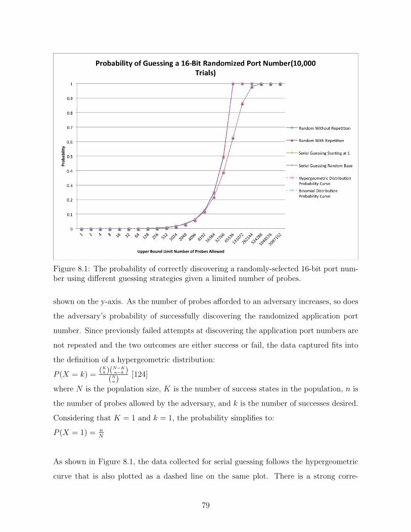
Figure 8.1: The probability of correctly discovering a randomly-selected 16-bit port num-ber using different guessing strategies given a limited number of probes.
shown on the y-axis. As the number of probes afforded to an adversary increases, so does
the adversary’s probability of successfully discovering the randomized application port
number. Since previously failed attempts at discovering the application port numbers are
not repeated and the two outcomes are either success or fail, the data captured fits into
the definition of a hypergeometric distribution:
P (X = k) =(Kk)(N−K
n−k )(Nn)
[124]
where N is the population size, K is the number of success states in the population, n is
the number of probes allowed by the adversary, and k is the number of successes desired.
Considering that K = 1 and k = 1, the probability simplifies to:
P (X = 1) = nN
As shown in Figure 8.1, the data collected for serial guessing follows the hypergeometric
curve that is also plotted as a dashed line on the same plot. There is a strong corre-
79

Figure 8.2: The average number of attempts expected before correctly discovering arandomly-selected 16-bit port number using different guessing strategies where the ad-versary is given a limited number of probes.
lation as the hypergeometric destination closely matches and overlaps the experimental
results collected. The effectiveness of the port randomization technique can be evaluated
based on the probabilistic results obtained for an adversary successfully discovering the
randomly-chosen port mapping given a certain number of probes allowed. For example,
allowing more than 215 probes would not be in the defender’s best interest since serially
guessing port numbers would give the adversary a probability of success above 50%. If it
is tolerable to allow a less than 5% chance of success, then the defender should consider
allowing 2048 probes as the upper bound limit placed on the adversary. Any amount of
probes above this limit would then be flagged and an operator would be alerted to take
the appropriate action to mitigate the threat. One example of a mitigation strategy an
operator can take would be to blacklist the adversary in a firewall rule so they can no
longer communicate on the network.
80

We also collected metrics on the average number of probes needed for an adversary to
learn the randomized port number. This average number is obtained when only consider-
ing the cases where the adversary successfully learned the correct randomized application
port number and is summarized in Figure 8.2. Since the serial guessing strategy follows
the hypergeometric distribution, the average number of attempts will continue to grow
until the expectation value is approximated (when there are ≥ 216 probes allowed by
the adversary). After that point, the number of attempts required remains constant as
the upper limit number of probes continues to increase. The expectation formula for the
hypergeometric distribution is as follows:
E(X) = N+1k+1
= N+12
= 32,768.5
Figure 8.3: The average amount of time needed before correctly discovering a randomly-selected 16-bit port number using different guessing strategies where the adversary isgiven a limited number of probes.
81

The average amount of time required per success, taken over all 10,000 trials, is shown in
Figure 8.3. For the serial guessing strategy starting at port number 1, the average time for
an adversary to successfully find the randomized port number is under 0.03 seconds when
the entire state space is explored. This upper bound time limit is attributed to the lim-
ited amount of entropy within a 16-bit space. Given the minimal amount of time required
for an adversary to discover the application port number by brute force, the frequency
at which a defender should re-randomize port numbers should be based on the number of
probes observed instead of solely based on time units alone. Within the small 0.03 second
window, ∼16,000 probes are injected by the adversary, which is a very noisy adversary
that can quickly be detected if the defender is monitoring the number of probes observed.
Additionally, the number of probes observed provides information to the defender on the
likelihood of success for an adversary, depending on how frequently the application port
numbers are being re-randomized as shown from Figure 8.1. Combining the information
on the success rate of the adversary along with the time required by an adversary until
a success can be expected provides the defender with the parameters necessary to protect
against adversaries who follow the strategies described.
8.1.2 Random Start, Serial Guessing
A similar adversarial strategy to discover application port numbers is where an adversary
starts at a random port number within the range of 1-65,536 and then incrementally at-
tempts subsequent port numbers until the correct randomized application port number
is found. Once the maximum port number value is reached by the adversary (65,536 in
this case), the port number overflows back to 1 and the adversary incrementally continues
guessing until the correct port number is found or until the original starting port number
is reached. The results of this strategy follow a similar pattern as the serial guessing
strategy since the defender chooses the random mapping uniformly at random and be-
cause the adversary starts scanning from a uniformly at random chosen initial application
port number. Because the application port number is chosen uniformly at random by
the defender, this adversary guessing strategy is equivalent to the case where the adver-
sary starts at application port number 1. Thus, there is no advantage from either the
82

adversary nor the defender when this guessing strategy is chosen. The success rates are
shown in Figure 8.1 verifying this result and also follow the hypergeometric distribution.
The hypergeometric plot significantly overlays the experimental results obtained and is
strongly correlated.
Since the serial guessing strategy with a randomly-chosen starting base for the appli-
cation port number also follows the hypergeometric distribution, the average attempts
needed until success similarly continues to grow until the expected value is approximated
(when there are ≥ 216 probes allowed by the adversary as shown in Figure 8.2). At this
point, the success rate remains constant as the number of attempts permitted by the
adversary continues to grow beyond the expectation value. The average amount of time
per success taken over all 10,000 trials also resembles the serial guessing strategy starting
at application port number 1 as shown in Figure 8.3. For the serial guessing starting at a
random base strategy, the average time for an adversary to successfully find the random-
ized port number is also under 0.03 seconds when the entire state space is explored. The
minimal amount of time required for an adversary to successfully discover the applica-
tion port number, again, provides guidance on the frequency at which a defender should
re-randomize application port numbers. The randomization frequencies should also be
based on the number of probes attempted by the adversary instead of solely based on
time units alone. The number of attempts that can be made within a 0.03 second period
is ∼16,000 attempts which is a large number of attempts and a fairly noisy adversary. The
defender can detect a high number of probes such as these by monitoring the incoming
and outgoing network traffic observed.
8.1.3 Random Guessing with Repetition
The next adversary strategy evaluated is when the adversary continuously probes appli-
cation port numbers selected uniformly at random until the correct randomized port has
been found. When using this strategy, it is possible that the adversary repeats previous
incorrect probes that were already made. Since previously failed probes can be repeated,
the probability of discovering the correct application port number from one attempt to
83

the next does not change. This is in contrast to the serial strategies discussed earlier
where the probability of success improved with each attempt since the pool of available
application port numbers continues to shrink with each attempt to find the correct ap-
plication port number. In this case, the probing strategy follows a binomial distribution.
As shown in Figure 8.1, the binomial distribution curve closely follows the experimental
results obtained for the random with repetition application port probing strategy and the
results are strongly correlated to the theoretical results. The probability function for the
binomial distribution is:
P (X = k) =(nk
)pk(1− p)n−k [125]
where N is the population size, p is probability of success, n is the number of probes
allowed by the adversary before the defender detects their presence, and k is the number
of successes desired by the adversary. In this case, it is of interest to find the probability of
at least one success which is equivalent to taking the complement of exactly zero successes
to simplify the formula above (k = 0):
P (X = k) = 1−(n0
)p0(1− p)n−0 = 1− (1− p)n
P (X ≥ 1) = 1− (1− p)n
Of the four strategies evaluated, this strategy is the least likely to be successful for an
adversary since repeating previously failed attempts are a possibility. The average num-
ber of probes needed for an adversary to learn the randomized application port number,
when only considering the successful cases, is summarized in Figure 8.2. Since the random
guessing with repetition strategy follows the binomial distribution, the average number
of attempts needed until a success occurs continues to grow until the expectation value is
approximated. In this case, the curve levels out to a constant value when there are ≥ 220
probes permitted by the adversary. The expectation formula for the number of attempts
before the first success is as follows:
E(X) = 1p
= 11
216= 65,536
84
The average amount of time required per success, taken over all 10,000 trials, is shown in
Figure 8.3. The average amount of time for an adversary to successfully find the random-
ized application port number is under 0.16 seconds when the entire state space is explored.
Comparing these results to the other strategies which take on average 0.03 seconds, this
strategy is 433% times slower until the first success is encountered. However, this upper
bound time is fairly minimal at 0.16 seconds and again is attributed to the limited amount
of entropy available within the state space of a 16-bit application port number. Given
the small amount of time needed by an adversary to successfully discover the randomized
application port number, the frequency at which the defender should re-randomize port
numbers is advised to be based on the number of probes observed rather than on the
amount of time that has passed. Monitoring the number of probes (∼30,000 in this case)
would provide sufficient information to detect the presence of an adversary.
8.1.4 Random Guessing without Repetition
The final guessing strategy analyzed is when an adversary randomly guesses application
port numbers without repeating any previously failed random probes. To implement such
a strategy, the adversary must track previously failed attempts to avoid repetition. To
succeed in this scenario, the adversary must discover the application port number before it
is remapped by the MTD strategy, based on a user configurable randomization frequency
parameter. This strategy once again maps to the definition of a hypergeometric distri-
bution and the data collected from the experimental results obtained verifies this mapping.
The three guessing strategies for an adversary that follow the hypergeometric distribution
(Serial Guessing; Random Start, Serial Guessing; and Random Guessing without Repeti-
tion) perform similarly with one another in terms of their success rates. The data collected
for each of these three strategies overlap one another significantly and are summarized in
Figure 8.1. The average attempts required until a successful attempt is encountered by an
adversary grows until the expectation value is approximated. This occurs when there are
≥ 216 probes allowed by the adversary as shown in Figure 8.2. When permitting more than
the expectation number of attempts by the adversary, the success rate remains constant.
85
The average amount of time per success taken over all 10,000 trials also resembles both
of the serial guessing strategies as shown in Figure 8.3. For the random guessing without
repetition strategy, the average time for an adversary to successfully find the randomized
port number is again under 0.03 seconds when the entire state space is explored. The
small amount of time required for an adversary to discover the application port number
again provides guidance on the frequency at which a defender should re-randomize the
application port numbers. The re-randomization intervals should be based on the num-
ber of probes observed rather than solely based on time units alone. If a relatively short
amount of time is configured to re-randomize application port numbers, such as every 1
second, then a rather noisy adversary could easily probe the network 65,536 and could
effectively defeat the MTD strategy. Since the results depend on the entropy available
to a defender, randomizing IP addresses produces similar results when 8 bits of both the
source and destination IP addresses are randomized.
8.2 Summary
The simulated environment we developed provided us with the ability to quickly collect
theoretical results during the early phases of our research on the feasibility of each MTD
approach. We were able to simulate four adversarial strategies and the MTD techniques
with stand-alone programs. The stand-alone programs allowed us to easily modify the
network parameters being simulated as part of each MTD technique as well as the adver-
sary strategies. Our findings were that an adversary can brute force a 16-bit application
port number (or 16-bits from a pair of IP addresses) in under 0.03 seconds with three of
the adversary strategies and within 0.16 seconds when one of the adversary strategies is
applied. This is a minimal amount of time for any of the four strategies but what works
against the adversary is the number of probes required to be successful. The adversary
must search at least half of the attack space before the first successful discovery of a
randomized 16-bit application port number can be discovered. Considering that there
are at least 16-bits of entropy available to the defender, the adversary must make 215
probes before the first success is expected. Figure 8.1 and Figure 8.2 show the two curves
86

that provide information on the success rates of an adversary given a variable number of
probes and the number of probes an adversary must attempt before the first successful
randomized mapping is discovered. Combining the information on the success rate of the
adversary along with the time required by an adversary until a success can be expected
provides the defender with the parameters necessary to protect against adversaries who
follow the strategies described. These results were later verified in both the virtualized
and representative environments developed that are discussed in the following chapters.
87

Chapter 9
Virtualization Environments
We developed a virtualized environment to validate the prior results obtained from the
simulated environment. The virtualized environment introduces the network communi-
cations into the experiments that were not present in the simulated environment. Open-
Flow version 1.3 is the protocol used to facilitate the communications between the SDN
controller and the SDN capable switches. A separate wrapper program manages the
randomized flows that are sent to the SDN controller which are then inserted into the
network. The mininet tool was used to build a network of virtual machines represent-
ing the end hosts of an ICS environment as well as the SDN capable switches. This
environment included the MTD strategies built-in to each of the virtual machines to
demonstrate the concepts beyond simulation. Open vSwitch was the software package we
chose to implement the SDN capable switches within the virtualized environment. Open
vSwitch provides the same functionality of a physical network switch in hardware, but it
is implemented in software where the randomization algorithms have been placed. It has
previously been shown that OpenFlow has the ability to randomize IP addresses within
a network as a standalone solution in a small scale network [20]. Additionally, it has also
been shown that overlay networks can be used to mitigate DDoS attacks [31]. One of the
goals of our research is to build upon these results by merging IP randomization, port
randomization, and overlay networks to counter the reconnaissance phase of an attack all
contained within a single solution.
88

Figure 9.1: A diagram of an example network where host A wishes to communicate withhost B. The OpenDaylight controller inserts flows within the overlay network so that pack-ets have randomized source and destination IP addresses, randomized port numbers, andtake random paths (shown as the red and green lines through overlay network) throughthe network.
The SDN network we used for our experiments operated under the open source Open-
Daylight controller [98]. The OpenDaylight controller communicates to the Open vSwitch
instances through the OpenFlow version 1.3 protocol to install the necessary flows to man-
age the randomized network parameters. The OpenDaylight controller is responsible for
installing flows that translate real IP addresses to randomized IP addresses when a packet
is traversing each of the Open vSwitch instances within the network. The OpenDaylight
controller also manages the randomized paths that the packets take through the overlay
network. Figure 9.1 depicts an example network where the OpenDaylight controller is
communicating with the Open vSwitches in the overlay network. The OpenDaylight con-
troller injects randomized source and destination IP addresses, randomized port numbers,
and randomized paths into the SDN overlay network when packets originating from host
A are sent to host B. The randomized source and destination IP addresses are trans-
lated back to the original source and destination IP addresses at the last hop switch
before reaching the final destination host B. Since the true IP addresses are mapped
to randomized IP addresses when entering the network and then re-mapped back from
89

Figure 9.2: The RTT measured across 10,000 pings with port randomization disabled andenabled.
the randomized IP addresses to the true IP addresses when the packets are leaving the
network, the solution is completely transparent to the end devices within the network.
9.1 Application Port Randomization Overhead Cost
Port randomization is implemented using the iptables [126] firewall tool that is built
into most Linux base installations. The performance impacts that result from using the
iptables rule chain to randomize application port numbers increased the latency by an
average of 0.015 ms and did not interrupt active communication sessions that were already
in progress. The results over a 10,000 second (∼2.77 hours) interval are shown in Figure
9.2. It should be noted that there is little to no performance impact of enabling port ran-
domization given that the maximum impact to the Round Trip Time (RTT) was within
1.2 ms of when port randomization was disabled which is well within the constraints of
a typical ICS environment. The strict timing constraints used within ICS environments
are noted to be no more than between 12-20 ms of additional delay.
90

The impacts on bandwidth when port randomization is enabled and disabled are shown in
Figure 9.3. We configured the port randomization updates to re-randomize all application
port numbers ranging from port numbers 1-1024 at a frequency of once every 10 seconds.
The iperf3 tool was used to gather the resulting data points over a 10,000 second (∼2.77
hours) interval. We observed a 9.91% reduction in bandwidth when port randomization
was enabled. The increase in overhead is attributed to the time to process each packet
in software and rewrite the application port numbers before forwarding and receiving
packets. There are typically not strict requirements on bandwidth and throughput mea-
surements within ICS environments since the communications usually require minimal
amounts of bandwidth.
Figure 9.3: The bandwidth measured across a 10,000 second (∼2.77 hours) period of timewhen application port number randomization is disabled and enabled.
9.2 IP Randomization Overhead Costs
The overhead cost incurred by the SDN switches to lookup the appropriate flow rules
and make the appropriate routing decisions (and rewriting source and destination IP ad-
dresses) resulted in an average of 0.04 ms of additional delay. We configured these lookups
only at the edge switches so that the operational impacts are well within the constraints of
91

a typical ICS environment of 12-20 ms [127]. We also performed experiments to validate
that the connectivity was maintained and uninterrupted between hosts actively commu-
nicating before, during and after each of the randomization periods. The verification of
the uninterrupted communication channels is important since high availability is one of
the primary requirements and concerns for an ICS environment. Availability is a concern
when introducing any new technology, security related or not, into the system. The re-
sults of sending 10,000 ping packets across a network are shown in Figure 9.4. We took
measurements when IP randomization was disabled and then again when it was enabled
on the network. The majority of the measurements collected overlap one another, in both
cases of when IP randomization was enabled or when it was disabled. The increases in
RTT that occur every 500 seconds when IP randomization is enabled typically do not
increase the RTT to more than 15 milliseconds and in the worst case do not increase
more than 30 milliseconds. The latency introduced falls within the bounds of the more
strict constraints (that range in milliseconds) the majority of the time and are well within
relaxed constraints (that range in seconds) of ICS environments.
Figure 9.4: The RTT measured across 10,000 pings when IP randomization is disabledand enabled.
92

Figure 9.5: The average bandwidth measured over a 10,000 second (∼2.77 hours) periodwhen IP randomization is disabled and enabled.
We also captured bandwidth measurements with and without IP randomization enabled.
The results are as expected in that when IP randomization is enabled, the bandwidth
measurements observed slightly decreased. This decrease is a result of the overhead in-
volved in the SDN flow rules, that when matched, must rewrite both the source and
destination IP address fields at the ingress and egress points in the network instead of
simply forwarding packets as a traditional switch would. However, traditional switches
occasionally require layer 2 traffic, such as ARP traffic, to learn about the locations of
new hosts that are introduced into the network. The overhead associated with rewriting
the IP address fields in an SDN deployment degrades the bandwidth as shown in Figure
9.5. The iperf3 tool was used to measure and capture the results over a 10,000 second
(∼2.77 hours) period of time.
The average bandwidth was reduced from 9.31 Gbits/sec to 9.14 Gbits/sec, or a 1.79%
decrease in performance. There is a significant amount of overlap when comparing IP
93

Figure 9.6: The average throughput measured over a 10,000 second (∼2.77 hours) periodof time when IP randomization is disabled and enabled.
randomization enabled and disabled. Also of note are the fluctuations when IP random-
ization is enabled that occur every 500 seconds. This is attributed to purge-times within
the OpenDaylight controller (the purge-times flush all flows and are part of the default
configuration) that happen every 500 seconds. When all rules are purged, there are slight
increases in delay because the Open vSwitch instances are forced to consult with the SDN
controller on how to appropriately route the packet. The purge-time is a user configurable
parameter that can be adjusted if desired, but the default value was not modified for these
experiments. Also of note is that ICS environments are typically not driven by bandwidth
and throughput measurements, but those metrics are captured here for potential ICS high
bandwidth scenarios, such as the case when communicating synchrophasor data.
We also evaluated the impacts on the total amount of data transferred over 10,000 second
(∼2.77 hours) intervals using the iperf3 tool when IP randomization was disabled and
then when it was enabled. As shown in Figure 9.6, the impacts on the amount of data
transferred are similar to the bandwidth measurements captured and described above.
94

The total data transferred can be viewed as another way to look at the bandwidth mea-
surements previously captured, but in terms of the amount of total data transferred over
each 1 second interval. The total amount of data transferred without IP randomization
enabled over the 10,000 second (∼2.77 hours) period is 10,834 GB. This number drops to
10,649 GB when IP randomization is enabled, or a 1.79% drop in performance. The drop
is attributed to the added time to overwrite the source and destination IP address fields
of the flow rules that are installed at each of the Open vSwitch instances.
Figure 9.7: The average bandwidth measured over a 10,000 second (∼2.77 hours) periodwhen IP randomization is disabled and enabled.
We also captured bandwidth metrics when using the Modbus protocol, a widely used
protocol within ICS environments. In this scenario, a Modbus server was running on a
single system and a Modbus client was running on a separate system that is programmed
to request 25 million reads of data. The results of the bandwidth metrics captured when
using the Modbus protocol are summarized in Figure 9.7. When IP randomization is not
enabled, the bandwidth on the 25 million reads is an average of 3,737 Kbits/sec. When IP
randomization is enabled, only a small decrease in bandwidth results in 3,525 Kbits/sec,
95

or a 5.67% decrease in performance. The delays observed are within the bounds of an
ICS environment and make the techniques feasible for deployment when using the Mod-
bus protocol.
Figure 9.8: The probability of correctly discovering a randomly-selected 24-bit number (aCIDR class A IP Address) using different guessing strategies given a limited number ofprobes.
Finally, we captured the probability distributions for adversaries who have the goal of
discovering the randomized source and destination IP addresses using different strategies
similar to the application port randomization techniques described earlier. The results are
shown in Figure 9.8 and are similar to those shown for the port randomization test per-
formed in Figure 8.1. We have verified that all strategies, except for random guessing with
repetition, follow the hypergeometric distribution over 10,000 trials of experiments that
model an adversary attempting to guess both of the randomized source and destination
IP addresses. In these sets of experiments, the assumption is that 24-bits are available to
96

use as host bits. Using 24-bits of the IP address as host bits provides an upper bound of
the effectiveness of the IP randomization technique given that it is unlikely, in practice,
to have a Classless Inter-Domain Routing (CIDR) class A network available within an
IPv4 address space, but could well have very large spaces with IPv6 addressing. The
random guessing with repetition strategy follows the binomial distribution and again is
verified through the experimental results obtained. As shown in Figure 9.8, the adversary
gains a better than 50% chance of success when allowed more than 223 attempts. This
is much improved from the application port randomization technique, however as previ-
ously mentioned, it is difficult to obtain a CIDR class A address space with 24-bits of
entropy available within an IPv4 environment. Conversely, within an IPv6 deployment,
IP randomization becomes more valuable since the IP space is much larger at 128 bits.
The expected number of probes required for an adversary to successfully discover the
24-bit host portion of the IP address behaves similarly to the port randomization. For
the random with repetition strategy, the binomial distribution curve matches the experi-
mental data captured. The average number of probes needed for an adversary to find the
randomized source and destination IP addresses, when only considering the success cases,
is summarized in Figure 9.9. In the binomial distribution, the average attempts needed
until success continue to grow until the expectation value is approximated, in this case,
when there are ≥ 224 probes allowed by the adversary:
E(X) = 1p
= 11
224= 16,777,216
When the adversary is allowed to make additional attempts, beyond the expectation value,
to find the randomized source and destination IP addresses, the success rate remains con-
stant.
The remaining strategies evaluated all follow the hypergeometric distribution and the
average grows until the expectation value is approximated. The expected number of
guesses until success for the remaining strategies is thus ≥ 224+12
probes. If the adversary
is allowed additional attempts beyond the expectation value, their success rate will again
97

remain constant. The defender should limit the adversary well below the expectation
number of probes when deploying each MTD technique. The result of the expectation
value leveling out the experimental data captured can be seen in Figure 9.9.
Figure 9.9: The expected number of attempts to randomly find a 24-bit number (a CIDRclass A IP Address) using different guessing strategies given a limited number of probes.
9.3 Path Randomization Overhead Cost
We implemented the path randomization technique by first capturing the network topol-
ogy and configuration. The topology and configuration knowledge required to initialize
the path randomization algorithms are the IP addresses of each host, the connections of
each host, the ports of the SDN switches, and the datapath id that uniquely identifies
each SDN switch in the network. The next step was to learn all possible paths between
each of the pairs of nodes using the Breadth First Search (BFS) algorithm [128] on the
network topology. Once all possible paths are known, the SDN controller then selects each
of the paths randomly from the exhaustive list of all paths and install the appropriate
98

flows to activate those paths so that all endpoints can communicate. The randomized
paths remain active for user configurable intervals. The intervals for the results shown as
part of our research are configured to install new random paths every 10 seconds.
The path randomization MTD approach introduced the most latency of the three chosen
MTD techniques, as shown in Figure 9.10. The RTT increased from 50 ms in a normal
configuration to 61 ms with path randomization enabled. When we enabled path random-
ization, data transfer rates and bandwidth rates were not affected but these parameters
are usually not of concern in ICS settings since these networks typically communicate
small messages. The time to transfer a 1 MB file had the largest increase in time from
70 ms using traditional switches to 100 ms when path randomization was enabled within
an SDN deployment.
Figure 9.10: Performance metrics of a normal network without randomization techniquesintroduced, with the three randomization algorithms implemented independently, andfinally with all three algorithms combined and applied.
The delays observed are attributed to the additional hops that are taken in the randomly-
chosen path that go beyond the optimal path in the network. In practice, this technique
would have to be throttled, similar to a QoS type of service to meet the potential real-time
constraints of the system that the technology is being applied towards. One of the main
goals of this MTD strategy is to prevent an adversary from discovering the endpoints
99
within a network by performing traffic analysis. The path randomization implementation
was developed using the POX controller since we developed these algorithms in the early
stages of our research. We also implemented the IP and port randomization schemes in
the POX controller to compare the same metrics against the path randomization metrics.
Our goal was to further reduce the overhead costs of each of the MTD techniques, which
the OpenDaylight controller satisfied as shown in Figure 10.7. The path randomization
algorithms can also be developed so that only a specific or a limited set of desired paths
are available to the defender to deploy, but this feature was not included as part of our
research. This could help support load balancing and could also enforce a QoS policy to
meet the requirements of the given environment.
9.4 Port, IP and Path randomization
We combined the proof-of-concept POX and OpenDaylight implementations of the three
randomized schemes into a single solution. We set the period of time to re-randomize
each MTD defense to 1 second intervals and the SDN-capable switches were all synchro-
nized together in time. This implementation choice of synchronizing the MTD techniques
simplified the process of gathering consistent performance metrics across multiple trials of
experiments. For example, if two of the three MTD techniques re-randomized at different
points in time, the results would vary from one run to the next. Since all three implemen-
tations are synchronized to re-randomize at the same time, the results are repeatable. We
have also compared the performance metrics collected against a baseline network without
any randomization applied. The results are shown in Figure 9.10.
The RTT is the round trip time retrieved from sending an Internet Control Message
Protocol (ICMP) ping message from one host to another and receiving back a response.
The baseline network without any of the MTD techniques enabled was the fastest, fol-
lowed closely by each of the individual MTD schemes enabled. The differences when each
MTD technique is individually enabled and disabled is the time it takes to lookup the
random port mappings, the time to overwrite the source and destination IP addresses,
100

the time to take additional hops through the network, and the management overhead
of the algorithms in a single centralized POX or OpenDaylight controller. The amount
of data transferred, in the second set of measurements, which we measured over a ten
second period were similar for each of the scenarios evaluated. The large amounts of data
transferred that we observed are due to the small scale network that mininet simulated,
all residing on a single machine with minimal network latency. Also, the Open vSwitch
instances did not have to ARP to repopulate internal tables to learn the locations of the
systems in the network which saved time when comparing against traditional switches.
The bandwidth reported also had similar results to the data transferred over a ten second
period. The 1 MB file transfers varied in latency when combining the three randomization
schemes. Port randomization increased in time because of the management required to
maintain and remap application port numbers within iptables. The IP randomization
further increased in time due to the fact that each packet had to be matched for the
source and destination IP addresses and the source and destination IP addresses had to
be rewritten if a match was made. The path randomization scheme, individually, in-
creased the most due to the additional hops required to be taken through the network.
The combination of all three randomization techniques yielded the largest amount of time
increases required for an attacker due to the cumulative overhead costs of each indepen-
dent technique combined. The metrics we collected, outside of the RTT, were produced
using the iperf3 tool.
Although the performance was impacted for each individual approach (as well as the
combined approaches), the transfer times of a 1 MB file are still faster than the average
rates that the Tor project is reporting, shown in Figure 9.11. Tor is a traffic anonymizer
which is an alternative to introducing IP randomization into a network. Tor is reporting
approximately five seconds to complete a 1 MB transfer on average, while the randomiza-
tion schemes proposed as part of our research are all under one second. This difference
comes from the fact that Tor requires additional processing time for the extra hops taken
in the Tor network plus the encryption and decryption overhead of each encapsulated
101

Figure 9.11: Performance metrics when transferring 1 MB files within the Tor networkover a three-month period of time.
portion of a packet. The Open vSwitch instances must only make a match on the fields
within the header of a packet, then potentially rewrite the source and destination IP
addresses, and finally forward the packet. The Open vSwitch costs shown as part of our
research are much lower than the cost of an encryption or decryption routine that the Tor
tool is reporting.
9.5 Summary
The virtualized environment we developed served as an intermediate step between the
simulated and representative environments. It was not known that we would have access
to a representative environment until later in the research, so we developed a virtual-
ized environment. We created virtual machines with the necessary software installed to
create a virtualized SDN network with the MTD techniques built-in. We then captured
operational metrics to evaluate the impacts to latency, bandwidth, throughput, and to
the Modbus protocol. We observed the impacts of IP randomization to latency to be
102

within 1.2 ms. This increase in time is well within the constraints of a typical ICS envi-
ronment, which are between 12-20 ms. Although most ICS systems are not bandwidth
and throughput driven, we captured these metrics in the event that there are large bursts
of traffic, such as when synchrophasor data is being communicated. We measured the
decreases in bandwidth and throughput when IP randomization was enabled to both be a
1.79% decrease. The percentages are not large and show the potential for these concepts
to be applied within other environments outside of ICS. We observed the impacts on
Modbus communications to drop by 5.67% on the number of reads and writes that could
be performed.
We again evaluated the four types of adversaries and we observed similar results as the
simulated results, but this time using virtual machines. It was verified that the adversary
would have to search, at a minimum, half of the attack space as was shown in the simulated
results. We also measured the application port number, IP address, and communication
path randomization schemes individually and in combination of each other. The MTD
scheme that incurred the largest amount of latency was the path randomization scheme.
This is due to the fact that the optimal path is not guaranteed to always be taken in the
network. The time for the additional hops increased the latency but also help prevent an
adversary from correlating endpoints based on traffic analysis. The path randomization
technique can also be further developed to restrict the maximum number of hops taken to
provide QoS guarantees to the users of the network. We observed that each of the MTD
techniques applied were feasible and well within the bounds of many ICS systems within
a virtualized environment.
103

Chapter 10
Representative Environments
We developed two representative environments to test and evaluate the MTD techniques
discussed previously in order to model different operational environments. The primary
goal is to capture effectiveness measurements of the MTD protections while also account-
ing for the operational traffic and processes running together that are difficult to provide
in simulated and virtualized environments. The two test environments include the DE-
TERLab testbed and an ICS testbed developed with both virtual and physical devices
that interact with each other. The DETERLab testbed provides physical systems and
network equipment that security researchers can allocate, customize, and configure for
security experiments. The environment is in a controlled isolated network so that the
tests can be made repeatable. The second environment is an ICS environment that is
also customizable and includes both physical and virtualized systems within the network.
The environment modeled is a virtual power plant that consists of ICS end devices and
protocols frequently deployed in operational ICS networks. Each environment and the
test results will be described in the sections that follow.
10.1 DETERLab Testbed
The cyber DEfense Technology Experimental Research Laboratory (DETERLab) testbed
hosts a network of physical computers and network devices where approved security re-
searchers around the world can test and evaluate new security technologies within a
controlled environment. The DETERLab testbed consists of over 600 physical computers
104

that can be allocated by security researchers to conduct computer security focused ex-
periments. Each computer can further instantiate up to 23 virtual systems per physical
system if larger experiments are needed. The computers vary in their processing power,
available memory resources, disk size and number of Network Interface Cards (NICs).
The network link speeds vary in capacity with a maximum of 10 Gigabits per Second
(Gbits/Sec) capable links. DETERLab1, based on the Emulab framework, and operated
by University of Southern California (USC) Information Sciences Institute (ISI) for the
purpose of security research, is under active development and is currently funded under
the Department of Homeland Security (DHS) within the Science and Technology (S&T)
Directorate.
The DETERLab was used to evaluate and analyze the tradeoffs between the increased
amount of adversarial workload incurred and the increased amount of operational im-
pacts imposed when IP randomization was enabled. We varied the frequencies at which
IP addresses are randomized as and also the number of adversaries attacking the IP ran-
domization scheme. The systems allocated within DETERLab for the IP randomization
experiments consisted of the following specifications:
• 2.13 GHz Intel R© Xeon R© CPU X3210 quad core processor
• 4 GB RAM
• 250 GB SATA Disk Drive
• Quad port Peripheral Component Interconnect Express (PCIe) Intel Gigabit Eth-
ernet card
• Ubuntu 16.04 64-bit
We configured each of the link speeds to 100 Megabits per second (Mbps) for all network
connections. In all experiments, the legitimate systems participating and supporting the
IP randomization are referred to as “operational nodes”. The systems attacking the
1DETERLab: https://www.isi.deterlab.net/
105

IP randomization scheme are referred to as “adversarial nodes”. For each experiment,
there are 4 operational nodes allocated to manage and run the IP randomization MTD
strategy and there are between 1 and 65,536 (or 216) adversarial nodes that have the
goal of defeating the IP randomization MTD scheme. We ran the experiments within
the DETERLab testbed with up to 32 physical adversarial nodes. The experiments that
had more than 32 adversarial nodes were simulated in our standalone system, since the
simulated results from Chapter 8 were consistent with the DETERLab results. Another
reason we chose to simulate the experiments that had more than 32 adversarial nodes
allocated was because of the DETERLab testbed physical resource limitations on the
number of nodes that had the same specifications at the time that the experiments were
performed. DETERLab currently supports a total of 64 nodes with the specifications
listed above, and each experiment was configured to consist of 4 operational nodes plus
2n adversarial nodes, where 0 ≤ n ≤ 16. Thus, the maximum number of physical nodes
that can be allocated given the constraints of 2n adversarial nodes plus 4 operational
nodes are experiments that consist of 32 adversarial nodes and 4 operational nodes. An
example of an experiment with 16 adversarial nodes and 4 operational nodes is shown
in Figure 10.1 for reference.
In Figure 10.1, each experiment network includes links that connect all of the nodes
to a single switch, labeled lan0. The switch supports the SDN technology to manage the
flows within the network. The network flows are the rules applied to each SDN switch
that are responsible for routing packets based on the criteria that is specified by the end
user. In this case, the rules specify to correctly route the packets to their destination
and also to randomize the source and destination IP addresses. The system responsible
for managing the network flows is called the SDN controller and is labeled nodeD and is
shown on the left side of Figure 10.1. The nodes labeled nodeA-nodeC are operational
nodes that represent the end users that are connected to the network. In this case, all
end users have a direct connection to the SDN controller so that IP addresses can be
randomized and de-randomized as packets leave and enter their NIC, respectively. Each
106

Figure 10.1: An experiment allocated within the DETERLab testbed consisting of 16adversarial nodes labeled nodeE1-nodeE16 and 4 operational nodes labeled nodeA-nodeD.
107
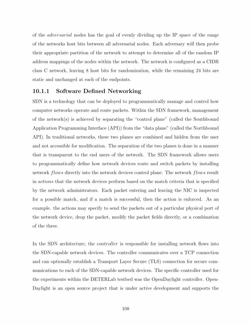
of the adversarial nodes has the goal of evenly dividing up the IP space of the range
of the networks host bits between all adversarial nodes. Each adversary will then probe
their appropriate partition of the network to attempt to determine all of the random IP
address mappings of the nodes within the network. The network is configured as a CIDR
class C network, leaving 8 host bits for randomization, while the remaining 24 bits are
static and unchanged at each of the endpoints.
10.1.1 Software Defined Networking
SDN is a technology that can be deployed to programmatically manage and control how
computer networks operate and route packets. Within the SDN framework, management
of the network(s) is achieved by separating the “control plane” (called the Southbound
Application Programming Interface (API)) from the “data plane” (called the Northbound
API). In traditional networks, these two planes are combined and hidden from the user
and not accessible for modification. The separation of the two planes is done in a manner
that is transparent to the end users of the network. The SDN framework allows users
to programmatically define how network devices route and switch packets by installing
network flows directly into the network devices control plane. The network flows result
in actions that the network devices perform based on the match criteria that is specified
by the network administrators. Each packet entering and leaving the NIC is inspected
for a possible match, and if a match is successful, then the action is enforced. As an
example. the actions may specify to send the packets out of a particular physical port of
the network device, drop the packet, modify the packet fields directly, or a combination
of the three.
In the SDN architecture, the controller is responsible for installing network flows into
the SDN-capable network devices. The controller communicates over a TCP connection
and can optionally establish a Transport Layer Secure (TLS) connection for secure com-
munications to each of the SDN-capable network devices. The specific controller used for
the experiments within the DETERLab testbed was the OpenDaylight controller. Open-
Daylight is an open source project that is under active development and supports the
108

OpenFlow 1.3 protocol standard. The OpenDaylight controller communicates to each of
the SDN-capable network devices via the OpenFlow 1.3 protocol and the OpenDaylight
“Boron” release version 5.1 SR1 was used for this testing.
The SDN-capable network devices that we used were software implemented switches.
Each of the operational nodes had the appropriate software installed so that the controller
could communicate with them as if they were traditional network switches. The software
switches used for this portion of research comes from the Open vSwitch project. Open
vSwitch version 2.6 was used because it communicates using the OpenFlow 1.3 specifi-
cation which encompasses much of the SDN features including IPv4/IPv6 compatibility
and IP modification actions. Previous versions of OpenFlow may not be compatible with
commercial SDN products as many of them require the use of at least OpenFlow version
1.3.
10.1.2 Threat Model
Given the use of SDN, and the ability to randomize IP addresses, we assume that the
goals of an intelligent motivated attacker would be to commandeer the IP randomiza-
tion scheme and inject spoofed packets into the network with a valid pair of operational
source and destination IP addresses. The adversary may or may not wish to be stealthy
depending on their objective. Additionally, the adversary must find the correct source
and destination IP addresses before the IP addresses are again re-randomized at user
defined frequencies. The adversary must correctly learn both the source and destination
IP addresses since the network flows installed at each SDN-capable network device must
match on both addresses to correctly route traffic. The match criteria could be further
restrictive by also matching on the physical port that the packet was received on in ad-
dition to the IP source and destination addresses. The extra match criteria would then
require an adversary to tap into the link that is between the operational node and the
SDN-capable network switch to succeed. The physical port was not specified as part of
the match criteria in each of these tests to simplify the DETERLab experiments that
demonstrate the concept of an adversary injecting an unauthorized packet into the net-
109
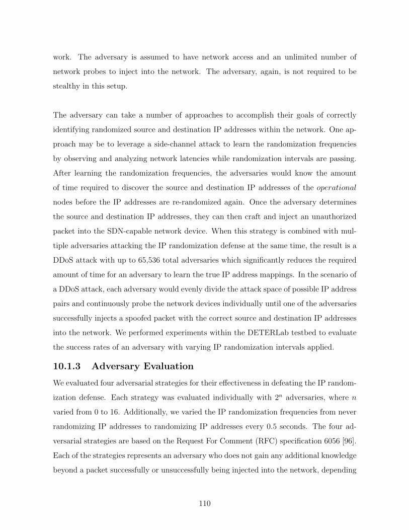
work. The adversary is assumed to have network access and an unlimited number of
network probes to inject into the network. The adversary, again, is not required to be
stealthy in this setup.
The adversary can take a number of approaches to accomplish their goals of correctly
identifying randomized source and destination IP addresses within the network. One ap-
proach may be to leverage a side-channel attack to learn the randomization frequencies
by observing and analyzing network latencies while randomization intervals are passing.
After learning the randomization frequencies, the adversaries would know the amount
of time required to discover the source and destination IP addresses of the operational
nodes before the IP addresses are re-randomized again. Once the adversary determines
the source and destination IP addresses, they can then craft and inject an unauthorized
packet into the SDN-capable network device. When this strategy is combined with mul-
tiple adversaries attacking the IP randomization defense at the same time, the result is a
DDoS attack with up to 65,536 total adversaries which significantly reduces the required
amount of time for an adversary to learn the true IP address mappings. In the scenario of
a DDoS attack, each adversary would evenly divide the attack space of possible IP address
pairs and continuously probe the network devices individually until one of the adversaries
successfully injects a spoofed packet with the correct source and destination IP addresses
into the network. We performed experiments within the DETERLab testbed to evaluate
the success rates of an adversary with varying IP randomization intervals applied.
10.1.3 Adversary Evaluation
We evaluated four adversarial strategies for their effectiveness in defeating the IP random-
ization defense. Each strategy was evaluated individually with 2n adversaries, where n
varied from 0 to 16. Additionally, we varied the IP randomization frequencies from never
randomizing IP addresses to randomizing IP addresses every 0.5 seconds. The four ad-
versarial strategies are based on the Request For Comment (RFC) specification 6056 [96].
Each of the strategies represents an adversary who does not gain any additional knowledge
beyond a packet successfully or unsuccessfully being injected into the network, depending
110

on if the correct source and destination IP address pairs were used. The hping3 tool
was used to craft and inject spoofed ICMP echo request messages into the network. If
an ICMP echo reply is observed in the network after the spoofed ICMP echo request is
sent, then the adversary would know that the source and destination IP addresses were
correctly spoofed, otherwise the IP addresses were incorrectly spoofed and they would
make another attempt with a different source and destination IP address pair. We used
the same adversary strategies that were presented for finding the application port num-
bers in Chapter 8 to find the IP addresses. The four strategies are summarized below, for
reference, along with the specific attacks that we crafted according to each strategy.
10.1.3.1 Random With Repetition
The first strategy evaluated is meant to model an adversary with minimal resources avail-
able and to attempt to avoid detection by observing patterns in the sequence of IP ad-
dresses spoofed. For this strategy, an adversary would first craft an ICMP echo request
packet with spoofed random source and destination IP addresses (selected uniform at
random) and then inject that packet into the network. If that attempted packet injection
fails to generate an ICMP echo reply from the spoofed destination system, then the ad-
versary would attempt to randomly probe the network again with a new set of randomly
selected source and destination IP addresses. The next random probe does not take into
account the previous attempts that have already failed, so it is possible that the source
and/or destination IP address will be repeated in this strategy. When there are multiple
adversaries attacking the IP randomization defense, the IP address space is divided evenly
into disjoint sets amongst all adversaries. Once a single adversary succeeds, the successful
adversary sends a message to all other adversaries to stop probing the network.
10.1.3.2 Random Without Repetition
The second strategy is similar to the first but does not repeat previously failed attempts of
incorrect source and destination IP address pairs. To avoid repeating previous attempts,
an internal table is maintained with all possible source destination IP address pairs. A
random permutation of that table is then generated and the adversary iterates through the
table to inject packets with the current spoofed source and destination IP address pairs
111

within the table. If the attempt fails, then the adversary injects a packet with the next
pair of spoofed source and destination IP addresses into the table. This process is repeated
until a packet is successfully injected into the network. When multiple adversaries are
involved, the IP address attack space is again divided up evenly into disjoint sets amongst
the adversaries. Each adversary follows the same strategy of first generating a random
permutation of the disjoint IP address space assigned to them followed by probing the
network with the current source and destination IP address pairs inserted into a ICMP
echo packet. All adversaries follow this strategy and simultaneously inject spoofed packets
until one of the adversaries is successful. An adversary knows when they are successful
because they will receive an ICMP response back after the spoofed packet is injected
into the network. If no successes are encountered before the adversary(ies) exhaust the
permutation table, then a new permutation is generated and the adversary(ies) restart
the process as before. This process continues until at least one adversary is successful.
10.1.3.3 Serial Probing
The serial probing strategy is another strategy that starts by initializing a 16-bit number
to 0. The first 8 bits of the 16-bit number represent the source IP address and the
second 8 bits represent the destination IP address. Packets are spoofed and injected into
the network with the supplied source and destination IP addresses based on the value
of the 16-bit number. The 16-bit number is continuously incremented until the correct
randomized source and destination IP address pairs are found. If the correct source
and destination IP address pairs are not found due to the IP randomization scheme re-
randomizing values of source and destination IP addresses during the network probing
process to a value that was previously attempted by the adversary, then the adversary
will be required to restart the same strategy from the beginning. When there are multiple
adversaries participating in a DDoS attack, the 16-bit number will be divided evenly into
disjoint sets amongst all adversaries, and the same process will be repeated until one
of the adversaries succeeds in finding the correct randomized source and destination IP
address pairs.
112

10.1.3.4 Serial Probing Starting at a Random Base
The final strategy is similar to the serial probing strategy, but instead of always starting
the 16-bit number at 0, a randomly-chosen 16-bit value is chosen as the starting point.
From the random starting point, the same process is continued where the adversary
incrementally probes the network for source and destination IP address pairs sequentially
by splitting the 16-bit value in half. If the source and destination IP address pairs are
not found after exhaustively searching the entire attack space for IP addresses (due to
the IP randomization scheme re-randomizing values to a previously probed source and
destination IP address pair), then the adversary would restart the process by selecting
a different randomly-chosen starting point. Similarly, if multiple adversaries exist, then
the attack space for IP addresses would be divided into disjoint sets for each adversary to
attempt to inject spoofed source and destination IP address pairs into the network. If a
response is received after the spoofed packet is injected, then the adversaries would know
that they have succeeded in spoofing a valid source and destination IP address pair. The
same process would continue until one of the adversaries successfully discovers the correct
randomized source and destination IP address pairs.
10.1.4 Results
We performed experiments within the DETERLab testbed using the previously described
adversary strategies. These are, of course, not the only adversary strategies that can
be developed, but these strategies were used as a baseline. Each experiment consists of
operational nodes with IP addresses that are randomized and adversarial nodes that
have the goal of discovering the randomized IP addresses assigned to a pair of nodes so
that a spoofed packet can be injected into the network. Because an SDN deployment is
used and flows are installed to match on both the source and destination IP addresses,
the adversary must find the combination of both addresses in the spoofed packet to be
successful. The experiments are performed so that an adversary continues to probe the
network using one of the four adversarial strategies until the correct source and destina-
tion IP addresses are found. Once the correct pair of IP addresses are successfully found,
the number of attempted probes is recorded and the experiment is repeated for another
113

trial. Each experiment is performed over 10,000 trials.
While each probe is being injected into the network, the IP addresses are at the same
time being re-randomized periodically by the defender. The frequencies at which the IP
addresses are being re-randomized by the defender range from never randomizing (the
minimum frequency that can be chosen) to randomizing every 0.5 seconds (the maximum
frequency chosen for our research). The specific intervals chosen for these experiments
include re-randomizing IP addresses every 0.5 seconds, 5 seconds, 10 second increments
starting from 10 and going all the way up to 260, and finally every 2m second intervals
where 0 ≤ m ≤ 20. The number of adversaries is also varied for each randomization
interval tested to evaluate the effects of a DDoS attack.
During a DDoS attack, the adversarial nodes will stop probing the network once a single
adversary succeeds. Since DETERLab makes use of the Network File System (NFS), all
adversarial nodes communicate, if they have succeeded, to the other adversarial nodes
by writing a “1” to a specific file on the NFS share. Each of the adversarial nodes checks
if this file has a “1” before injecting each new probe into the network. Once all adversarial
nodes learn that one of the other adversarial nodes have successfully found the correct
source and destination IP address pairs, they wait until they can synchronize with each
other to repeat the same test in another trial. Each experiment was run through 10,000
trials to ensure that a high enough statistical significance was achieved to yield a 99% level
of confidence with a ± ∼1.3% margin of error in the experimental results obtained. The
formula used to calculate the statistical significance of a sample size needed to achieve a
99% confidence level with a ∼1.3% margin of error:
n = z2×p(1−p)e2
= 2.582×0.5(0.5)1.292
=10,000
where n is the sample size, z = 2.58 is the normalized value of where 99% of the cumu-
lative normal distribution, p = 0.50 is the proportion of values above the mean number
of probes, and e = 1.29% is the margin of error. The value of p was chosen as 50%
since the distribution of the resulting number of probes needed until success is normally
114
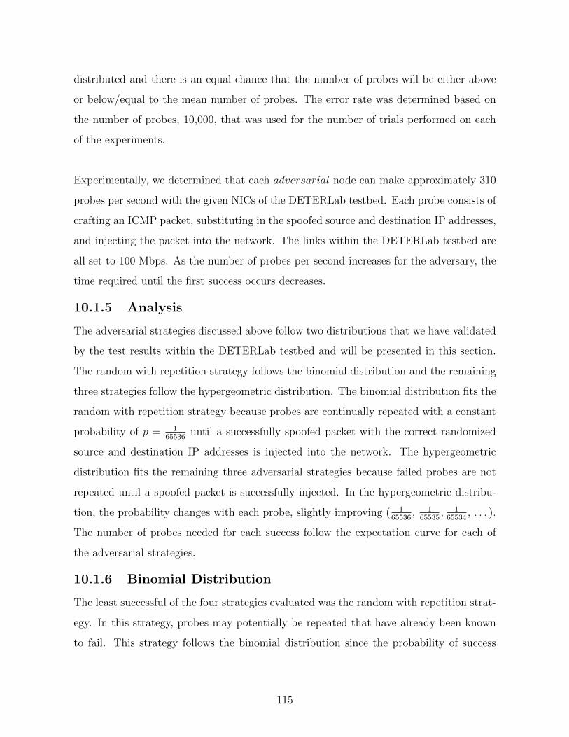
distributed and there is an equal chance that the number of probes will be either above
or below/equal to the mean number of probes. The error rate was determined based on
the number of probes, 10,000, that was used for the number of trials performed on each
of the experiments.
Experimentally, we determined that each adversarial node can make approximately 310
probes per second with the given NICs of the DETERLab testbed. Each probe consists of
crafting an ICMP packet, substituting in the spoofed source and destination IP addresses,
and injecting the packet into the network. The links within the DETERLab testbed are
all set to 100 Mbps. As the number of probes per second increases for the adversary, the
time required until the first success occurs decreases.
10.1.5 Analysis
The adversarial strategies discussed above follow two distributions that we have validated
by the test results within the DETERLab testbed and will be presented in this section.
The random with repetition strategy follows the binomial distribution and the remaining
three strategies follow the hypergeometric distribution. The binomial distribution fits the
random with repetition strategy because probes are continually repeated with a constant
probability of p = 165536
until a successfully spoofed packet with the correct randomized
source and destination IP addresses is injected into the network. The hypergeometric
distribution fits the remaining three adversarial strategies because failed probes are not
repeated until a spoofed packet is successfully injected. In the hypergeometric distribu-
tion, the probability changes with each probe, slightly improving ( 165536
, 165535
, 165534
, . . . ).
The number of probes needed for each success follow the expectation curve for each of
the adversarial strategies.
10.1.6 Binomial Distribution
The least successful of the four strategies evaluated was the random with repetition strat-
egy. In this strategy, probes may potentially be repeated that have already been known
to fail. This strategy follows the binomial distribution since the probability of success
115

with each attempted probe does not change. Since there are 8 bits of randomness in each
of the source and destination IP addresses, the total number of bits of entropy available
are 16 bits. In this case, the adversary(ies) have a 165536
chance of success on each and
every probe. If the entropy increased by using a CIDR class B network, the same curve
would result, but requiring more attempts by the adversary until a successful randomized
source and destination IP address is found.
Figure 10.2: The solid lines represent the number of attempted spoofed packets that needto be injected into the network with varying frequencies of re-randomizing IP addresses.As the randomization frequencies increase in time, the number of required attemptedadversary spoofed packets before a successful packet is injected decreases. The dashedlines represent the theoretical expectation results of the binomial distribution, whichmatch the experimented data closely. Each of the curves represents the total number ofadversaries, varying from 1 adversary to 65,536 adversaries. The frequency intervals varyfrom 0.5 seconds to a static configuration. We performed 10,000 trials with an adversarythat was capable of injecting 310 packets per second in the test environment provided.
116

The graph in Figure 10.2 shows the results of varying numbers of adversaries probing the
network with varying frequencies of randomization on the IP addresses. We performed
these tests within the DETERLab testbed. Each of the solid line curves represents a dif-
ferent number of adversaries probing the network and the average number of probes (per
adversary) needed before their first success across 10,000 total trials. The dashed lines
that follow the curve are the expectation curves that are validated from the experiments
performed within the DETERLab testbed. Because the distribution here is binomial,
it follows that the expected number of probes for the random variable x until the first
success follows the formula:
E(x) = 1p
When a single adversary is probing the network, the adversary must probe the full 16-bit
IP space before the first success is expected to occur. This is attributed to the fact that the
probability is constant across all probes, in this case p = 165536
, no matter how many probes
have already been injected into the network. Thus, the expectation is E(x) = 1p
=65,536.
When there are two adversaries probing the network, the IP space can be divided in half
(p = 132,768
) making the expectation curve become E(x) = 1p
=32,768. As the number
of adversaries double, the expectation constant curve requires half the total number of
expected probes per adversary. This process was repeated until there was a total of 65,536
adversaries, in which case only a single probe is needed by each adversary until a success is
found since there is one adversary assigned to each of the possible IP address assignments.
10.1.7 Hypergeometric Distribution
The most successful adversarial strategies followed the hypergeometric distribution. The
probes of the adversaries in these strategies either repeatedly select source and destination
IP addresses randomly without repetition, serially guess IP addresses starting from 0, or
serially guess IP addresses starting at a random base. Since the definition of the hyperge-
ometric distribution states that previous failed attempts are not repeated, it follows that
each of the strategies fits the definition of the hypergeometric distribution. The graphs
in Figures 10.3 - 10.5 show the results obtained from the DETERLab testbed. All of the
117

graphs are similar to one another and are strongly correlated with each of the associated
hypergeometric expectation curves, shown as dashed lines.
Figure 10.3: The hypergeometric distribution is followed when the adversary randomlyspoofs the source and destination IP addresses until a success occurs without repeatingprevious failed attempts. The results captured experimentally match those of the expec-tation curve when varying the number of adversaries and the frequencies at which thedefender re-randomizes the network IP addresses.
Focusing on Figure 10.3, the top curve shows the data obtained for a single adversary
probing the network and attempting to inject a packet into the network with a forged
randomly-chosen source and destination IP address. Since our experiments operate within
a CIDR class C network address space, there are 8 bits of entropy for each of the source
and destination IP addresses. Because the adversary must successfully guess the correct
source and destination IP addresses in order to successfully inject a packet into the net-
work, the problem is equivalent to an adversary finding a randomly-chosen 16 bit number
118

without repeating previously failed attempts as shown in the simulated results in Chapter
8. If the adversary does not guess both correctly, the packet will be dropped since the
network is an SDN based environment that requires flow rules to match both the source
and destination IP addresses in order to route a packet. The values along the x-axis
of the graph show the increase in the amount of time for the defender to re-randomize
the current set of active IP addresses within the network. The y-axis shows the average
number of probes needed by the adversary, over 10,000 trials, until the first successful
packet is injected into the network. When randomizing IP addresses frequently (between
0.5 seconds to 10 seconds), the adversary must attempt ∼65,535 probes before the first
success occurs (on average). As the defender randomizes IP addresses less frequently (>
210 seconds), the adversaries’ number of probes is cut in half to ∼32,768 (on average)
probes before the first successful packet is injected into the network. The curve is linear
and is dependent upon the frequency at which an adversary can re-randomize IP addresses
and the number of probes/second an adversary can inject into the network.
In the DETERLab testbed we observed that ∼310 packets/second can be crafted, forged
with the source and destination IP addresses, and then injected into the network. These
metrics come from the open source tool hping3. The network connections all operate
with 100 Mbits/second capacity links. Therefore, when randomizing every 0.5 seconds,
the adversary is capable of injecting ∼ 310 × 0.5 ≡ 155 packets per second into the
network. Given the expectation formula from the hypergeometric distribution, the first
success would be encountered E(X) = N+12
= 65,536+12
=32,768.5, where N is the popu-
lation/attack space. Since the adversary cannot make unlimited probes into the network
before the IP addresses are re-randomized, the expectation formula must be modified to
model the moving IP address targets as well as the continuous stream of probes com-
ing from the adversary. The probability of success, with a restricted number of probes
before the IP address changes is p = k/N , where k is the number of packets injected
into the network with spoofed source and destination IP addresses. Thus, the prob-
ability of failing to inject a packet with the correct pair of source and destination IP
119

Figure 10.4: The hypergeometric distribution is followed when the adversary seri-ally spoofs the source and destination IP addresses (starting at IP addresses X.Y.Z.0-X.Y.Z.255, where X, Y and Z are 8 bit octets of an IP address) until success. The resultscaptured experimentally match those of the expectation curve when varying the numberof adversaries and the frequencies at which the defender re-randomizes the network IPaddresses.
120

Figure 10.5: The hypergeometric distribution is similarly followed when the adver-sary serially spoofs the source and destination IP addresses (starting at IP addressesX.Y.Z.[random mod 256]-X.Y.Z.[random mod 256-1], where X, Y and Z are 8 bit octetsof an IP address and random mod 256 is a randomly-chosen number between 0 and 255through the modulo operator) until success. The results captured experimentally matchthose of the expectation curve when varying the number of adversaries and the frequenciesat which the defender re-randomizes the network IP addresses.
121

addresses given k probes is p = 1 − p = 1 − k/N . To find the expectation of an adver-
sary after repeatedly probing the network k times over and over again before the first
success occurs, given that the IP addresses are re-randomized every k probes, the expec-
tation function then becomes: the original expectation of the hypergeometric distribution
plus the original expectation of the hypergeometric distribution multiplied by the num-
ber of failed attempts before the first success. The second part of the formula accounts
for the number of failed attempts before the first success is found when limited to k
probes before IP addresses are re-randomized. More simply, the formula can be written
as E(X) = N+12
+ N+12× (p) = N+1
2+ N+1
2× (1− k/N) = N+1
2× (1 + p). This expectation
formula is shown in the curve as a dashed line in Figure 10.3. As shown, the expecta-
tion curve has a strong correlation with the data collected from within the DETERLab
testbed. The shape and pattern of the curve continues regardless of the number of adver-
saries probing the network. The only change in the formula is the attack space since the
adversaries are evenly dividing up the workload.
10.2 Virtual Power Plant
The Virtual Power Plant (VPP) environment, developed at Sandia National Laborato-
ries [129], is a representative ICS system that includes several virtual machines as well as
physical systems found within an ICS setting. The network topology of the VPP envi-
ronment is shown in Figure 10.6. The virtual machine systems are shaded in red and the
physical systems are shaded in blue. The operating systems of the virtual machine in-
stances we used were Linux Ubuntu installs running control system software. The network
includes several inverters (systems that changes direct current (DC) to alternating current
(AC)), power generators, smart meters, battery energy storage systems (BESS), servers
that would be found within a control system, and the necessary routing and switching
equipment for end devices to communicate over the network. We applied the IP ran-
domization, port randomization and fault tolerant algorithms towards this environment
in order to measure the effectiveness of each MTD strategy within a representative ICS
environment and to validate the simulated and virtualized results captured in Chapter 8
122

and Chapter 9, respectively.
Figure 10.6: A representative ICS environment that combines both virtual and physicalenvironments to model a power plant using ICS-based systems and protocols.
In this scenario, we used the systems labeled as Engineering Workstation, Historian,
SCADA Server, General HMI, and OPC to manage the MTD techniques. We placed
the SDN controller instances on each of these systems to push and install flows to each
of the SDN-capable switches in the network. The SDN-capable switches in the network
were configured to be Open vSwitch instances. A wrapper program with knowledge of
the network topology was written to communicate with the controller to install new flows
into the network. The protocol used to communicate between the controller and the Open
123

vSwitch instances is OpenFlow version 1.3.
We implemented each of the virtual machine instances in the environment as separate
isolated virtual machines as shown in red. The physical systems and inverters that were
connected with the virtual environment are shown in blue. The end hosts configured to
communicate with each other in this scenario were the systems labeled as Inverters and
the BESS systems. These systems communicated over the SDN and Open vSwitch fabric.
This was done so that no additional configuration on the end hosts were needed so that
the solution could be transparent to each of the end hosts. The IP randomization was
enabled, using IPv4 and IPv6 protocols. We then captured the performance metrics while
these systems communicated with one another in a similar manner to an operational ICS
environment.
The second set of tests we performed to evaluate the resiliency of the controller were
in the events of either a crash or a maliciously modified Open vSwitch instance to incor-
rectly route traffic. We applied crash tolerant and Byzantine fault tolerant algorithms to
show that the single point of failure found in SDN deployment with a single controller
could support failover controllers without downtime and with minimal impacts to the op-
erational network. Performance metrics were then captured to demonstrate the feasibility
of applying the fault tolerant algorithms to improve the resiliency of the SDN controllers.
The OpenDaylight controller was used for these experiments, but any controller could
have been substituted as long as it implemented the OpenFlow 1.3 protocol. The Byzan-
tine Fault Tolerant State Machine Replication (BFT-SMaRt) [130] algorithm was used
to proxy the fault tolerant algorithms to protect the flows that were being installed from
attempted compromises on any of the individual controllers.
We performed all experiments while the systems in the VPP environment continuously
communicated with one another using standard ICS protocols including the Transmission
124
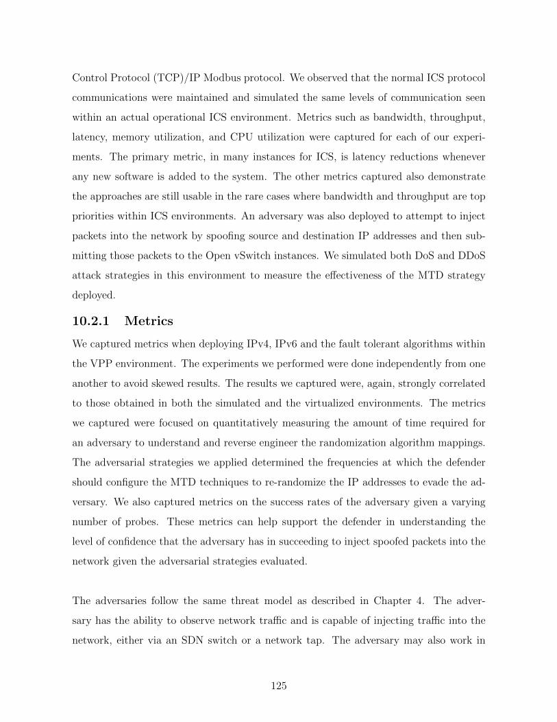
Control Protocol (TCP)/IP Modbus protocol. We observed that the normal ICS protocol
communications were maintained and simulated the same levels of communication seen
within an actual operational ICS environment. Metrics such as bandwidth, throughput,
latency, memory utilization, and CPU utilization were captured for each of our experi-
ments. The primary metric, in many instances for ICS, is latency reductions whenever
any new software is added to the system. The other metrics captured also demonstrate
the approaches are still usable in the rare cases where bandwidth and throughput are top
priorities within ICS environments. An adversary was also deployed to attempt to inject
packets into the network by spoofing source and destination IP addresses and then sub-
mitting those packets to the Open vSwitch instances. We simulated both DoS and DDoS
attack strategies in this environment to measure the effectiveness of the MTD strategy
deployed.
10.2.1 Metrics
We captured metrics when deploying IPv4, IPv6 and the fault tolerant algorithms within
the VPP environment. The experiments we performed were done independently from one
another to avoid skewed results. The results we captured were, again, strongly correlated
to those obtained in both the simulated and the virtualized environments. The metrics
we captured were focused on quantitatively measuring the amount of time required for
an adversary to understand and reverse engineer the randomization algorithm mappings.
The adversarial strategies we applied determined the frequencies at which the defender
should configure the MTD techniques to re-randomize the IP addresses to evade the ad-
versary. We also captured metrics on the success rates of the adversary given a varying
number of probes. These metrics can help support the defender in understanding the
level of confidence that the adversary has in succeeding to inject spoofed packets into the
network given the adversarial strategies evaluated.
The adversaries follow the same threat model as described in Chapter 4. The adver-
sary has the ability to observe network traffic and is capable of injecting traffic into the
network, either via an SDN switch or a network tap. The adversary may also work in
125

parallel with other adversaries to create a DDoS attack to more efficiently attack the
system. The defender also has the ability to observe and react to noisy adversaries. This
is handled by modeling the number of probes afforded to an adversary before detection.
After a certain configurable number of attempts are made by the adversary, the defender
has the ability to prevent the adversary from continuing to make progress in their exploits.
The results obtained help determine the feasibility of the MTD approaches being in-
troduced into the ICS environments and also help learn the tradeoffs associated with each
approach. We have parametrized each of the MTD approaches developed so that the
MTD techniques negatively impact on the operational ICS environment are minimized.
The MTD parameters can be adjusted according to the unique sets of constraints and re-
quirements that are required for each ICS environment. The implementations and results
for each of the MTD approaches are described in the sections that follow.
10.2.2 IPv4
The VPP environment supports both IPv4 and IPv6 protocols. The majority of tests we
performed using IPv4 addresses were consistent with the simulated and virtualized results.
Additionally, we captured latency, throughput, CPU, and memory metrics for the IPv4
sets of experiments. In these experiments, we integrated physical switches such as the HP-
2920 and the SEL-2740 SDN capable switches into the environment to measure latency,
bandwidth and dropped packets within a representative environment. We configured
the switches to interoperate with the OpenDaylight controller and received flows with
randomized source and destination IP addresses to be installed at each of the SDN-capable
switches.
10.2.3 Operational Impacts
One of our primary goals in applying the MTD techniques to the VPP environment was
to introduce a minimal or zero amount of additional latency into the system. High avail-
ability is typically the top priority for an ICS environment. We captured latency metrics
within the VPP environment when varying the frequencies at which IP randomization
126

occurs. The round trip times were also captured over a 1,000 second interval and those
times were averaged separately for each of the randomization frequencies applied.
Figure 10.7: The latency impacts of varying the frequencies of randomization from astatic configuration to randomizing once every second. As the randomization frequenciesincrease in time, the latency measurements decrease.
The results are shown in Figure 10.7. The randomization frequencies varied between a
static environment (IP randomization disabled) to as frequent as every 1 second. The
static configuration of IP addresses without using SDN had the largest amount of latency
out of the group. This has been attributed to the time required to periodically com-
municate Layer 2 protocols, such as ARP, for hosts within the network and because the
proactive (instead of reactive) flows are installed on each switch. With proactive flow
rule installation, the flows being pushed to each of the switches is initiated by the SDN
controller. If the SDN network was configured in a reactive flow rule installation setting,
127

then the controller would be consulted on each packet received. The proactive flow rule
installation process allows provides each switch, immediately, with the knowledge of how
to route each packet received and is responsible for the speed-up observed. The SDN
implementation did not have the overhead of looking up and populating an ARP table
when sending and receiving packets. As shown in the metrics captured, the more frequent
the randomization intervals become, the more delay there is on latency. Randomization
intervals of 1 second resulted in a ∼0.65ms delay whereas randomizing every 1000 seconds
incurred a ∼0.55ms delay. All results we captured were within 1 ms of each other which
demonstrates the feasibility of these approaches to be applied within an ICS environment.
We also captured the TCP retransmits when varying the frequencies of randomization
from a static configuration to randomizing once every second as shown in Figure 10.8.
The retransmits were captured over a 10 minute interval where 500,037 packets in total
were transmitted. In general, as the randomization intervals increase, so do the rates of
TCP retransmits. The number of retransmits are attributed to the workload placed on
the Open vSwitch (OVS) instances during the randomization intervals where flows were
being added, removed, and updated.
For each of these metrics, two hosts (the BESS and the Inverter in the bottom left of
Figure 10.6) were communicating with one another through two Open vSwitches. All
other systems within the VPP environment continued to communicate with one another
normally to increase the load on the network. The network continued to operate as ex-
pected throughout these experiments and we observed no interruptions in connectivity
between any hosts within the network while the IP randomization strategy was enabled.
The IP randomization technique was configured to re-randomize source and destination
IP addresses every 1 second. An overlap window of 10 seconds was configured so that
each flow would remain on the Open vSwitches for an additional nine seconds after the 1
second period that they were active. After the 1 second active period expired, a new flow
with a new random source and destination IP address pair was installed. This was done
128
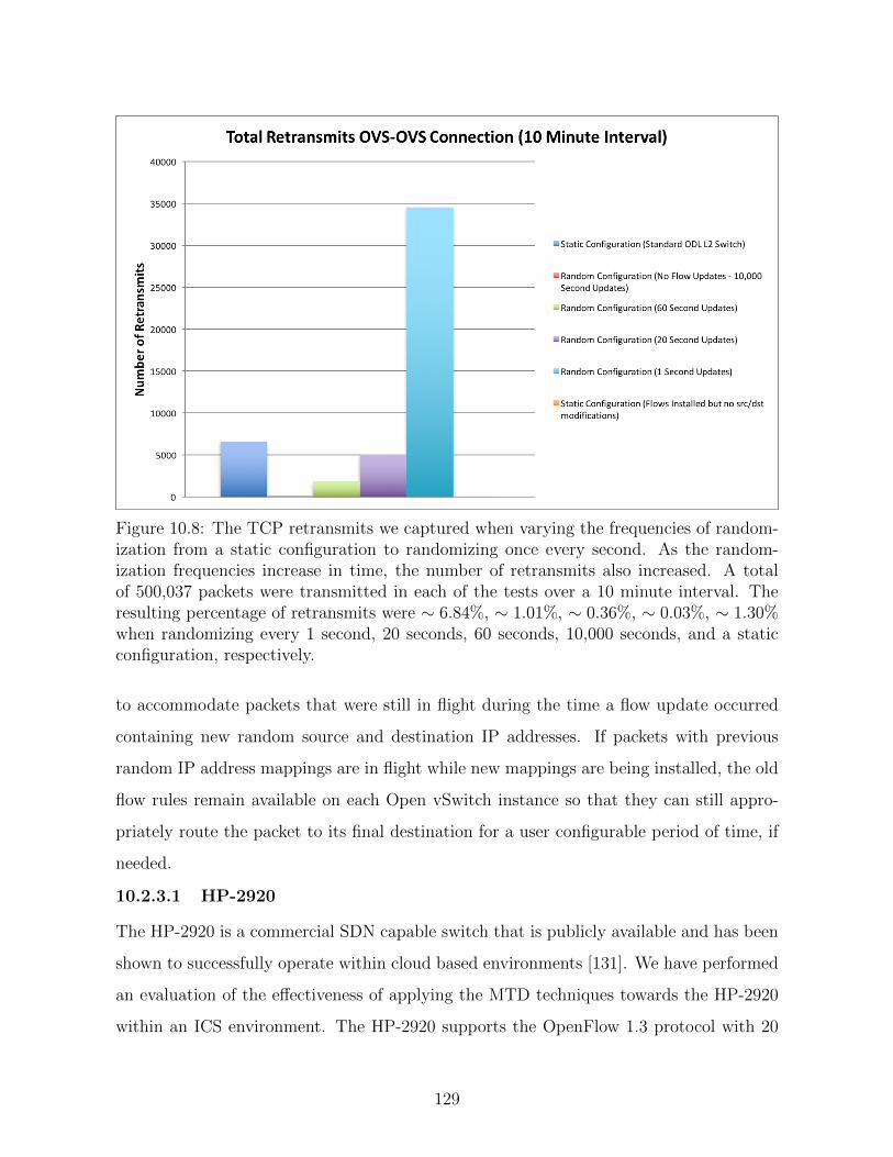
Figure 10.8: The TCP retransmits we captured when varying the frequencies of random-ization from a static configuration to randomizing once every second. As the random-ization frequencies increase in time, the number of retransmits also increased. A totalof 500,037 packets were transmitted in each of the tests over a 10 minute interval. Theresulting percentage of retransmits were ∼ 6.84%, ∼ 1.01%, ∼ 0.36%, ∼ 0.03%, ∼ 1.30%when randomizing every 1 second, 20 seconds, 60 seconds, 10,000 seconds, and a staticconfiguration, respectively.
to accommodate packets that were still in flight during the time a flow update occurred
containing new random source and destination IP addresses. If packets with previous
random IP address mappings are in flight while new mappings are being installed, the old
flow rules remain available on each Open vSwitch instance so that they can still appro-
priately route the packet to its final destination for a user configurable period of time, if
needed.
10.2.3.1 HP-2920
The HP-2920 is a commercial SDN capable switch that is publicly available and has been
shown to successfully operate within cloud based environments [131]. We have performed
an evaluation of the effectiveness of applying the MTD techniques towards the HP-2920
within an ICS environment. The HP-2920 supports the OpenFlow 1.3 protocol with 20
129

gigabit ports. The switch was evaluated in the test environment described above and
substituted in for one of the Open vSwitch instances in Figure 10.6. The HP-2920 switch
works by processing the flows in software when any packet modifications are desired.
The processing of the flows in software is performed on flows that have action rules that
go beyond simply forwarding packets out of a port. For example, rewriting source and
destination IP addresses would be performed in software since those flows make packet
modifications before forwarding the packet. Flows that only forward packets out of a port
are processed in hardware with significant performance improvements.
Figure 10.9: We captured latency measurements when sending traffic between two hostsusing two traditional switches forwarding traffic in the middle. Latency measurementswere also captured when two Open vSwitch instances replaced the traditional switcheswith varying randomization frequencies of IP addresses.
We measured the performance impacts of the software based implementation when the
IP randomization MTD technique is enabled. A comparison when two Open vSwitch are
routing traffic versus when an Open vSwitch and an HP-2920 switch route traffic has
been performed. Varying the frequency of randomization from a static configuration to a
130

1 second randomization window is shown in Figures 10.9 and 10.10. All frequencies are
within 10 ms of each other and are well within the bounds of an ICS environment.
Figure 10.10: Latency measurements captured when sending traffic between two hostswith two traditional switches forwarding traffic in the middle. Latency measurementswere also captured when one Open vSwitch instance and one physical HP-2920 switchreplaced a traditional switch with varying randomization frequencies of IP addresses.
The traditional switches, labeled “Static configuration (Stadard ODL L2 Switches)” in-
curred, on average, 2.309 ms of latency when using two Open vSwitch instances and, on
average, 1.562 ms of latency when introducing the HP-2920 switch. The HP-2920 switch
improved the latency metric in this case because the switching is performed in hardware.
When focusing on the data points obtained when the SDN configuration was initialized
to route traffic and matching rules are made without source and destination IP address
rewrites performed (the data points labeled “Static Configuration (Flows installed but
no src/dst modifications)”), the HP switch begins processing packets in software because
flow matching is performed on IP fields instead of MAC addresses only. The average la-
tency for the two Open vSwitches scenario is 0.740 ms and the average latency for the HP
131
switch paired with an Open vSwitch instance is 4.404 ms, or a 494% increase in latency,
on average. The Open vSwitch instances begin switching traffic faster in this scenario be-
cause ARPs are no longer needed to be communicated between endpoints. The increase
in time is not, however, significant enough, in this scenario, to impact an ICS network
beyond the limit of 12-20 ms.
When randomizing IP addresses and rewriting source and destination IP addresses at
10,000 second intervals, the average latency when using two Open vSwitch instances is
1.026 ms and 4.714 ms when using one Open vSwitch instance with the HP-2920 physical
switch. The 360% increase is again attributed to the software matching of the flow rules
performed within the HP-2920 switch. When randomizing at more frequent intervals, the
average latency for both cases of using two Open vSwitch instances or one Open vSwitch
instance paired with one HP-2920 switch are similar. In the scenario where two Open
vSwitch instances are deployed with randomization frequencies of 60 seconds, 20 seconds,
and 1 second, the average latencies are 0.728 ms, 0.711 ms, and 1.091 ms, respectively.
In the one Open vSwitch and one HP-2920 switch case with randomization frequencies of
60 seconds, 20 seconds, and 1 second, the average latencies are 4.366 ms, 3.941 ms, and
4.993 ms. The 1 second randomization frequencies have the largest impact on latency,
but are still within range of the desired 12-20 ms.
10.2.3.2 SEL-2740
We evaluated another publicly-available, commercial switch, the Schweitzer Engineering
Laboratories 2740 (SEL-2740) has been evaluated for latency impacts in a standalone net-
work. The tests were performed onsite at SEL so the only tests performed at the time were
latency tests and dropped packets. The Open Daylight controller was used and a secure
Transport Layer Security (TLS) [132] connection was established between the controller
and both of the SEL-2740 switches. The two SEL-2740 switches were directly connected
to each other. Each of the SEL-2740 switches had several end systems directly connected
to them and communicating using ICS specific protocols such as DNP3 and Modbus TCP.
132

We performed experiments with randomization frequencies of 60 second and 1 second
intervals. In each scenario, we configured 100 Mbits/second links with separate tests
performed with 1% and 99% link utilizations configured. With the 60 second random-
ization frequency configured and 1% link utilization, the latency introduced was 25.6
microseconds. When 99% link utilization was configured, the latency introduced was
80.6 microseconds. The large improvement in speed compared to the Open vSwitch and
HP-2920 switches is attributed to the flows being processed in hardware as opposed to
software.
When the randomization frequency was adjusted to 1 second intervals, the results were
similar to those obtained when randomizing every 60 seconds. When the link utilization
was set to 1% saturation, 25 microseconds of latency were incurred on the communication
channel. When the saturation level was increased to a 99% link utilization, the latency
increased to 87.8 microseconds. All latency metrics captured using the SEL-2740 switch,
which is specifically tailored towards ICS environments, were well within the constraints
of an ICS environment. Given the results of less than 1 ms of latency, the SEL-2740
can be applicable to a wide range of environments that have even more strict latency
constraints than a typical ICS environment.
We also examined the number of dropped packets in our experiments. The IP ran-
domization, with all varying frequencies, did not cause any packets to be dropped. All
switches evaluated including the HP-2920, the SEL-2740, and the Open vSwitch did not
drop any packets. This is an important metric specifically within an ICS setting. Dropped
packets may cause delays or major outages within the power grid, depending on if TCP
or UDP communications are used, respectively. These directly affect the general public
and in some cases, such as when hospitals depend on the power grid and energy delivery
systems, can be a cause for public health and safety concerns.
133

10.2.4 Fault Tolerance
The controller of an SDN network can be considered a single point of failure as mentioned
previously. If the controller fails or is compromised, then the SDN controller would no
longer be able to communicate with the SDN switches and the MTD randomization would
no longer continue to function. The network would then return back to a static configu-
ration and would lose the benefits of the MTD protections. To protect against the SDN
controller from becoming a single point of failure, intentional or not, we have designed
fault tolerant algorithms into the SDN controller. The effectiveness of each algorithm has
been captured with latency and bandwidth metrics experimentally captured within the
VPP environment.
We integrated both of the crash tolerant and Byzantine tolerant algorithms into the SDN
controller to protect it from having a system failure or from experiencing a compromise
within the flow configurations. To ensure that an operational SDN controller will still
be available in the event of SDN failures, we integrated the Paxos algorithms into the
SDN controller. The improved resiliency has been accomplished by allocating a cluster
of controllers to serve as failover systems and also by having consensus agreements on
the flows installed in the network. In this deployment, the single point of failure for the
SDN controller is eliminated when the Paxos algorithms are applied to track the status
of all of the controllers in the cluster. If an adversary is attempting to compromise the
SDN controller with the fault tolerant algorithms enabled, they now must compromise a
majority of the controllers in the cluster to be successful.
Similarly, we have integrated Byzantine fault tolerant algorithms into the SDN controllers
to protect the flows that they are communicating to the SDN-capable switches in the
network. In the event that one of the controllers is compromised and attempting to com-
municate false information to the rest of the cluster, the Byzantine algorithms will not
only detect the false information but will prevent other controllers from trusting the false
information. The Byzantine algorithms can ensure a consensus agreement and can toler-
134

ate f failures when there are 3f + 1 controllers installed within the cluster.
The fault tolerant algorithms combined with enabling the MTD techniques in an SDN
setting will have performance costs associated with them. ICS environments can only
tolerate minimal amounts of delay to the operational network and any new technology
introduced, including security protections, must be evaluated to meet the strict time con-
straints and requirements. We have captured latency, throughput, CPU, and memory
measurements for each of the fault tolerant algorithms combined with the MTD tech-
niques.
Figure 10.11: Latency metrics we captured within the VPP environment over a 1,000second interval of time. We captured these results to measure a baseline for the VPPenvironment.
135

Figure 10.11 shows the VPP environment running as a traditional ICS network without
the SDN framework, the MTD strategies or the fault tolerant algorithms enabled. The
average latency measured experimentally over a 1,000 second period of time is 0.612 ms.
We captured this baseline measurement of latency independently to compare against the
latencies captured when enabling each of the security protections separately within the
VPP environment.
Figure 10.12: Latency metrics captured within the VPP environment over a 1,000 secondinterval of time. The results show the effects of applying an SDN framework combinedwith the IP randomization MTD technique.
Next, we captured performance metrics when the IP randomization techniques were en-
abled within the VPP environment. The latency results captured over a 1,000 second
interval are shown in Figure 10.12. We configured the randomization frequencies to gen-
136

erate new random source and destination IP addresses every 1 second. The average
latency over the 1,000 second period of time improved from the traditional network base-
line previously captured as the SDN network does not require ARP requests and replies to
operate and because the proactive (instead of reactive) flows are already installed on each
switch before each packet is first observed. The latency captured for the round trip time
of an ICMP message was recorded as 0.546 ms, a 10.78% improvement in performance.
Figure 10.13: Latency metrics captured within the VPP environment over a 1,000 secondinterval of time. The results show the effects of applying the SDN framework combinedwith the IP randomization MTD technique and the Paxos crash tolerant algorithm.
To determine the performance impacts of the fault tolerant algorithms, we enabled the
crash tolerant algorithms and captured latency metrics within the VPP environment.
Figure 10.13 shows the results that build on Figure 10.12 where the IP randomization
137

technique is additionally enabled. In this case, we configured four controllers to be part
of the cluster of failover controllers to handle the event of crash related faults. The exper-
iment was setup so that every 250 seconds, one of the controllers from the cluster would
crash and no longer be responsive. The crash is meant to simulate an adversary exploit-
ing a controller one at a time and to measure the performance impacts during those time
periods when a failover occurs. As shown in Figure 10.13, connectivity is lost 500 seconds
into the experiment. This is caused due to the fact that at least half of the systems, 2 in
this case, in the cluster of 4 had crashed at that time (since the experiment was designed
for controllers to crash every 250 seconds). The Paxos crash tolerant algorithms require
a majority of the cluster to be responsive in order to have a consensus agreement which
is not possible when half of the controllers fail. The average latency measured when a
consensus agreement could be successfully reached was 0.542 ms, which is comparable to
the IP randomization algorithms running independently without the fault tolerant algo-
rithms enabled.
We then captured latency measurements when the Byzantine fault tolerant algorithms
were enabled. In this set of experiments, an individual flow residing on one of the con-
trollers was maliciously modified to route traffic to the adversary instead of to the origi-
nal destination endpoint. The Byzantine algorithms implemented could handle f failures
when there are 3f + 1 controllers. In this scenario, 1 failure can be tolerated since there
are 4 controllers configured within the cluster. Figure 10.14 shows the round trip time
measurements associated with the Byzantine fault tolerant algorithms and the IP ran-
domization enabled. The results are similar to those of the crash tolerant algorithms in
that communications discontinued after 500 seconds. After 2 failures, a consensus agree-
ment on the flows installed could no longer be achieved. The increased latency, as shown
in Figure 10.14, is attributed to the compromised controllers attempting to communicate
the malicious flow to the other controllers in the cluster and the other controllers waiting
for a consensus agreement amongst the cluster. However, since the other controllers are
also participating in the Byzantine fault tolerant algorithms, they detect the differences
138

in the malicious flows being communicated to them and reject those differences until a
consensus agreement can be achieved between the cluster. The spikes in latency after
every 250th packet show the additional communications taking place when the malicious
flows are sent. The average latency when we enabled all of the SDN framework, the IP
randomization, and the Byzantine fault tolerant algorithms was measured to be 0.587 ms,
which is also comparable to the VPP baseline.
Figure 10.14: Latency metrics captured within the VPP environment over a 1,000 secondinterval of time. The results show the effects of applying the SDN framework combinedwith both the IP randomization MTD technique and the Byzantine fault tolerant algo-rithms.
We also captured throughput measurements when the crash and Byzantine fault tolerant
algorithms were enabled. A baseline measurement was captured for the throughput over
a 1,000 second interval with a 10 Mbits/sec link configured. As shown in Figure 10.15, the
139
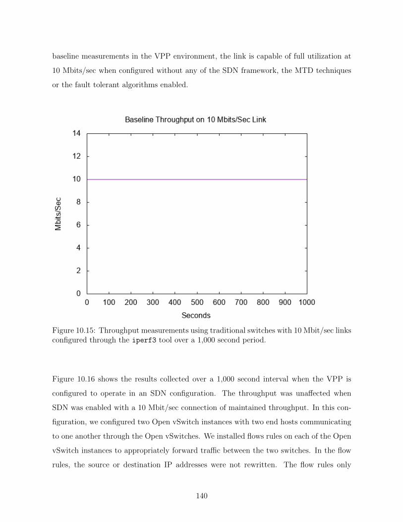
baseline measurements in the VPP environment, the link is capable of full utilization at
10 Mbits/sec when configured without any of the SDN framework, the MTD techniques
or the fault tolerant algorithms enabled.
Figure 10.15: Throughput measurements using traditional switches with 10 Mbit/sec linksconfigured through the iperf3 tool over a 1,000 second period.
Figure 10.16 shows the results collected over a 1,000 second interval when the VPP is
configured to operate in an SDN configuration. The throughput was unaffected when
SDN was enabled with a 10 Mbit/sec connection of maintained throughput. In this con-
figuration, we configured two Open vSwitch instances with two end hosts communicating
to one another through the Open vSwitches. We installed flows rules on each of the Open
vSwitch instances to appropriately forward traffic between the two switches. In the flow
rules, the source or destination IP addresses were not rewritten. The flow rules only
140

matched packets based on the incoming physical port and the source and destination IP
addresses before forwarding out the appropriate output port.
Figure 10.16: Throughput measurements using Open vSwitch instances that only forwardtraffic based on incoming physical ports, with 10 Mbit/sec links configured through theiperf3 tool over a 1,000 second period.
Figure 10.17 shows the throughput results captured in the VPP environment when IP ran-
domization is enabled. We obtained similar results from the baseline indicating that the
IP randomization and SDN framework do not have a noticeable impact on the through-
put observed within the VPP environment. These results are consistent with those dis-
cussed previously on the latency impacts of enabling both the SDN framework and the
IP randomization technique. Throughput is not typically a strong requirement for ICS
environments, except for potentially in the case where synchrophasor data is continuously
being communicated across the network which can require high amounts of bandwidth.
141

Figure 10.17: Throughput measurements using Open vSwitches that randomize sourceand destination IP addresses before forwarding traffic. Network links were configured tooperate at 10 Mbits/sec through the iperf3 tool over a 1,000 second period.
Figures 10.18 - 10.21 show the throughput measurements when the crash tolerant algo-
rithms are enabled within the VPP environment. The capture was performed over the
same 1,000 second interval of time with a 10 Mbits/sec link configured. In each of these
experiments, a controller was manually brought down to simulate an adversary causing a
crash in the controller every 250 seconds. The number of controllers in the cluster varied
between 2 controllers and 5 controllers.
142
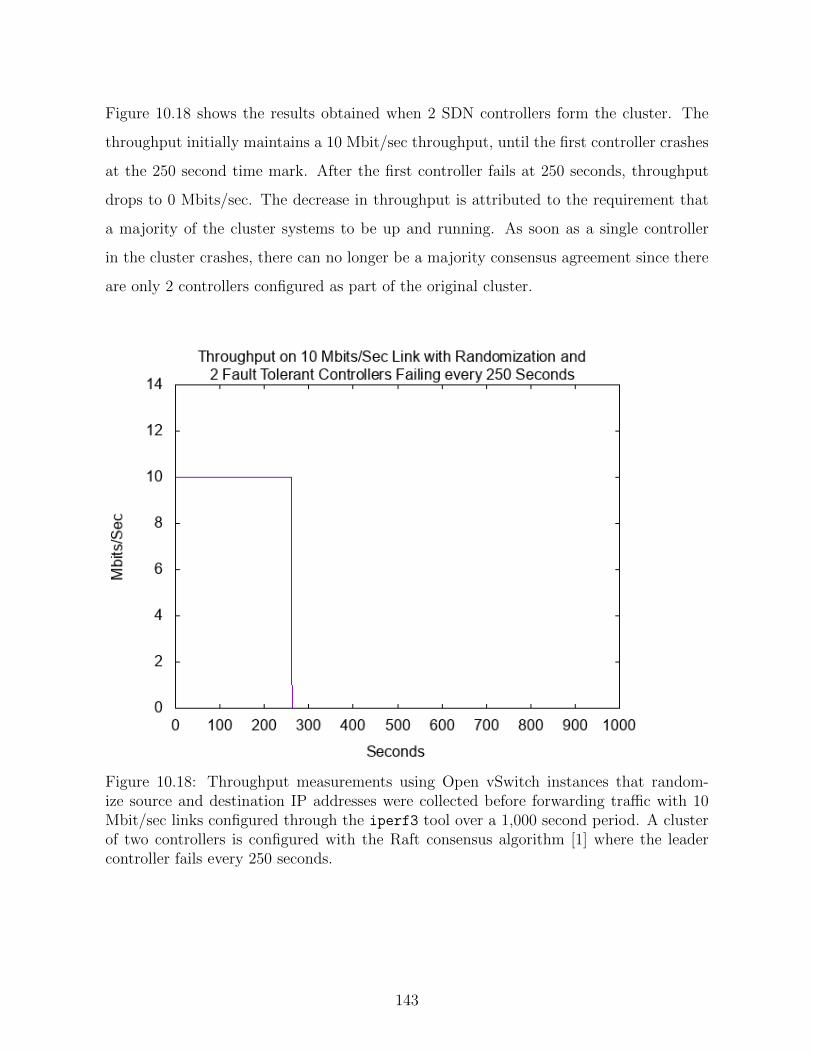
Figure 10.18 shows the results obtained when 2 SDN controllers form the cluster. The
throughput initially maintains a 10 Mbit/sec throughput, until the first controller crashes
at the 250 second time mark. After the first controller fails at 250 seconds, throughput
drops to 0 Mbits/sec. The decrease in throughput is attributed to the requirement that
a majority of the cluster systems to be up and running. As soon as a single controller
in the cluster crashes, there can no longer be a majority consensus agreement since there
are only 2 controllers configured as part of the original cluster.
Figure 10.18: Throughput measurements using Open vSwitch instances that random-ize source and destination IP addresses were collected before forwarding traffic with 10Mbit/sec links configured through the iperf3 tool over a 1,000 second period. A clusterof two controllers is configured with the Raft consensus algorithm [1] where the leadercontroller fails every 250 seconds.
143

Figure 10.19 shows the results obtained when 3 controllers form the cluster. The through-
put is maintained at 10 Mbit/sec, until 2 of the controllers crash at the 500 second time
mark. After the first controller failure occurs at 250 seconds, throughput is maintained at
10 Mbits/sec because a majority of the controllers, 2 in this case, are still up and running.
As soon as the second controller crashes, the throughput drops to 0 Mbits/sec. The drop
in throughput is attributed to the requirement that a majority of the cluster systems be
up and running. As soon as 2 out of 3 controllers in the cluster crash, there can no longer
be a majority consensus agreement.
Figure 10.19: Throughput measurements using Open vSwitch instances that randomizesource and destination IP addresses before forwarding traffic, with 10 Mbit/sec links con-figured through the iperf3 tool over a 1,000 second period. A cluster of three controllersis configured with the Raft consensus algorithm where the leader controller fails every 250seconds.
144
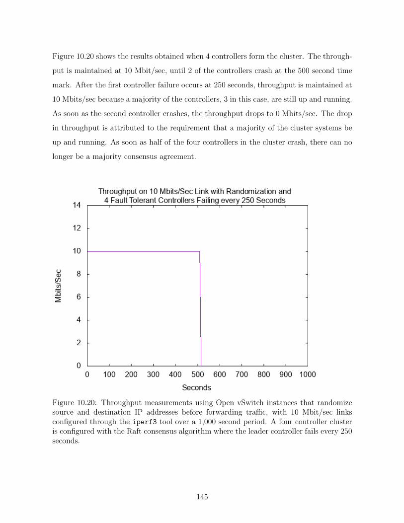
Figure 10.20 shows the results obtained when 4 controllers form the cluster. The through-
put is maintained at 10 Mbit/sec, until 2 of the controllers crash at the 500 second time
mark. After the first controller failure occurs at 250 seconds, throughput is maintained at
10 Mbits/sec because a majority of the controllers, 3 in this case, are still up and running.
As soon as the second controller crashes, the throughput drops to 0 Mbits/sec. The drop
in throughput is attributed to the requirement that a majority of the cluster systems be
up and running. As soon as half of the four controllers in the cluster crash, there can no
longer be a majority consensus agreement.
Figure 10.20: Throughput measurements using Open vSwitch instances that randomizesource and destination IP addresses before forwarding traffic, with 10 Mbit/sec linksconfigured through the iperf3 tool over a 1,000 second period. A four controller clusteris configured with the Raft consensus algorithm where the leader controller fails every 250seconds.
145

Figure 10.21: Throughput measurements using Open vSwitch instances that randomizesource and destination IP addresses before forwarding traffic, with 10 Mbit/sec linksconfigured through the iperf3 tool over a 1,000 second period. A 5 controller cluster isconfigured with the Raft consensus algorithm where the leader controller fails every 250seconds.
146

Figure 10.21 shows the results obtained when 5 controllers form the cluster. The through-
put is maintained at 10 Mbit/sec, until 3 of the controllers crash at the 750 second time
mark. After the first controller failure occurs at 250 seconds, throughput is maintained at
10 Mbits/sec because a majority of the controllers, 4 in this case, are still up and running.
When the second controller crashes at the 500 second mark, the cluster can still reach a
consensus agreement since a majority 3 out of 5 controllers are still up and running. As
soon as the third controller crashes, the throughput drops to 0 Mbits/sec. The drop in
throughput is attributed to the requirement that a majority of the cluster systems be up
and running. As soon as 3 or more of the 5 controllers in the cluster crash, there can no
longer be a majority consensus agreement.
The next set of metrics we captured are collected from the end devices that serve as the
SDN controllers. CPU and memory utilization measurements were captured to under-
stand the impacts to the SDN controllers themselves, which are responsible for installing
the appropriate flows on each of the SDN switches to correctly route traffic. We initially
performed the measurements to capture a baseline of the VPP environment, then also
when enabling the IP randomization techniques, then when also enabling the crash toler-
ant algorithms, and finally when enabling the Byzantine fault tolerant algorithms. The
specifications of the SDN controller systems are as follows:
• 2.60 GHz Intel R© Xeon R© CPU ES-2670 processor
• 1 GB RAM
• 20 GB SATA Disk Drive
• Gigabit Ethernet card
• Ubuntu 16.04 64-bit
147

Figure 10.22: CPU impacts on the SDN controller when deploying Byzantine fault tolerantalgorithms with IP randomization enabled, crash tolerant algorithms with IP randomiza-tion enabled, no fault tolerant algorithms with IP randomization enabled, and a baselinewith no fault tolerant algorithms and IP randomization disabled.
Figure 10.22 shows the CPU utilization impacts on the controllers over a 1,000 second
interval of time. All scenarios are plotted on the same graph to compare different mea-
surements easily. The lowest CPU impact came from the baseline CPU measurements
when the VPP was configured to run without any of the SDN, IP randomization, or fault
tolerant algorithms enabled. The average CPU utilization in that scenario was measured
to be ∼2.7%. When IP randomization is enabled, the average CPU utilization increases
to ∼10.3% utilization. When the crash tolerant and IP randomization algorithms are
enabled, the average CPU utilization becomes ∼20.4%. Finally, when the Byzantine and
IP randomization algorithms are enabled, the average CPU utilization is measured to be
∼20.7%.
148

The largest increase measured when we incrementally enabled new features was after
the fault tolerant algorithms were enabled. An additional ∼7.6% (on average) CPU uti-
lization was needed when enabling the IP randomization algorithms from the baseline
measurements. After enabling the fault tolerant algorithms, an additional (on average)
∼17.7% utilization was required for the crash tolerant algorithms and ∼17.9% for the
Byzantine fault tolerant algorithms. The fault tolerant algorithms were implemented in
Java and the Java Virtual Machine environment required 512 megabytes when it was
initialized. Although the endpoint controllers did experience a higher level of load on
the CPU, there were not significant degradations in latency and throughput as shown in
Figures 10.11 - 10.14 and Figures 10.17 - 10.21. Within an ICS environment, the fault
tolerant algorithms do not provide a significant amount of overhead and would be ap-
propriate to apply, provided that the controllers have similar specifications as described
previously. Outside of an ICS environment, the feasibility of applying the fault tolerant
algorithms will depend on the requirements of those environments as well as the other
processes that would also be running on the SDN controller. Isolating and separating the
controller onto its own standalone system may be an appropriate option if there are a
significant number of processes and applications hosted on the same system.
The memory overhead was also captured on each of the controllers within the cluster.
The metrics we captured were for a baseline configuration, when IP randomization was
enabled, when IP randomization combined with the Paxos crash tolerant algorithms were
enabled, and when IP randomization combined with the Byzantine fault tolerant algo-
rithms were enabled. The baseline memory consumption within the VPP environment
running without any of the security protections over a 1,000 second interval was measured
at ∼28.8% utilized on average. When enabling IP randomization, the crash tolerant algo-
rithms, and the Byzantine fault tolerant algorithms, the average memory usage increased
to 91.4%, 92.2%, and 92.6%, respectively. These results are reflected in Figure 10.23. The
reason for the large increase is due to the amount of memory required to initialize the
149

Figure 10.23: CPU impacts on the SDN controller when deploying Byzantine fault tolerantalgorithms with IP randomization enabled, crash tolerant algorithms with IP randomiza-tion enabled, no fault tolerant algorithms with IP randomization enabled, and a baselinewith no fault tolerant algorithms and IP randomization disabled.
Java Virtual Machine that is needed to start the OpenDaylight controller. The amount
of memory used within OpenDaylight was configured to be 512 megabytes, or half of a
gigabyte, which was the major contributor to the increase in memory usage. The large
memory requirements combined with the fact that the controllers each only had 1 giga-
byte of memory is the reason for the greater than 50% increases in memory usage. In an
operational setting, the memory requirements of the OpenDaylight controller should be
factored into the decision about the specifications chosen for that system. With the small
amount of memory available on the controller systems used in this set of experiments, the
memory was nearly at a maximum. This could cause delays in communicating new flows
to each of the switches in the network which would then potentially cascade into latency
150

increases.
10.2.5 IPv6
An evaluation of the IP randomization MTD technique using IPv6 addresses was per-
formed within the VPP environment. IPv6 was chosen to validate the simulated results
of the adversarial workload increases described in Chapter 9 for IPv4 and also to eval-
uate the feasibility and effectiveness of IPv6 within an ICS setting. IPv6 is currently
not widely deployed within ICS environments but researchers have been considering it
for inclusion for several years [133]. IPv6 is the successor of IPv4 and was designed to
expand on the limited amount of IPv4 addresses available [134]. IPv4 addresses consist of
32 bit addresses whereas IPv6 addresses consist of 128 bit addresses. The larger address
space provides additional entropy for the IP randomization scheme. As shown previously
in Chapter 9, an adversary can brute force a pair of CIDR class C IP addresses in under
0.03 seconds, which is a minimal delay for an adversary. Using IPv6 addresses allows
the defender to expand the entropy beyond the typical 8 bits of entropy that would be
customary in an IPv4 deployment. IPv6 addresses would typically have on the order of
64 bits available in many deployments [135] or 100× (256−1) percent more entropy. This
added entropy makes brute force techniques infeasible for an individual adversary.
We have captured metrics on the effectiveness of IPv6 randomization to evaluate the
impacts on the increased amount of workload placed on the adversary. We have also ana-
lyzed individual adversaries and distributed adversaries for their effectiveness in learning
the randomized IPv6 mappings. Our experiments within the VPP environment captured
the number of probes that an adversary must attempt before successfully reverse engi-
neering the randomized IPv6 addresses. The IPv6 addresses chosen contained 10 bits of
entropy on both the source and destination addresses. In our tests, we repeated each
experiment with 10,000 trials to verify that the results obtained from the IPv4 addresses
scaled similarly when expanding the IP address space.
151

10.2.6 Individual Adversaries
Figures 10.24 - 10.27 show the experimental results obtained within the VPP environ-
ment when an individual adversary attacks the IPv6 randomization schemes using the
four adversarial strategies described in Section 10.1.3 to reverse engineer the randomized
IPv6 addresses. The first strategy is to spoof randomly-chosen source and destination
IPv6 addresses continuously until a successful spoofed packet is injected into the network.
This process may potentially repeat previously failed attempts. The second strategy per-
forms the same strategy except a table is maintained to avoid repeating previously failed
attempts. The last two strategies scan IPv6 addresses sequentially, with the first of the
two starting with the first available IPv6 address and the second starting at a random
IPv6 address. The four strategies we used were taken from RFC 6056 [96].
The top most curves for each of the four strategies are shown in Figures 10.24 - 10.27
for an individual adversary attacking the system. The random with repetition strategy,
again, followed the binomial distribution. Since previous attempts may be repeated, the
probability from one probe to the next is constant and does not improve as more probes
are made. Figure 10.24 shows the constant curve and the expectation of 210+10 = 220
probes required until the first success that was experimentally encountered within the
VPP environment. The source and destination IPv6 addresses both had 10 bits of en-
tropy built in for a total of 20 bits of entropy combined.
The same analysis was performed when the adversary strategy was modified to randomly
probe the network with spoofed IPv6 addresses that did not repeat. The difference in
this strategy is that the adversaries’ probability will improve with each attempt since
previous attempts are not repeated. We varied the randomization frequencies in these
experiments and the intervals are shown along the x-axis of Figure 10.25. As the random-
ization frequencies increase in time going to the right on the curve, the success rate of the
adversary improves. This is attributed to the environment remaining statically configured
for longer periods of time which allows the adversary to probe the network longer before
152
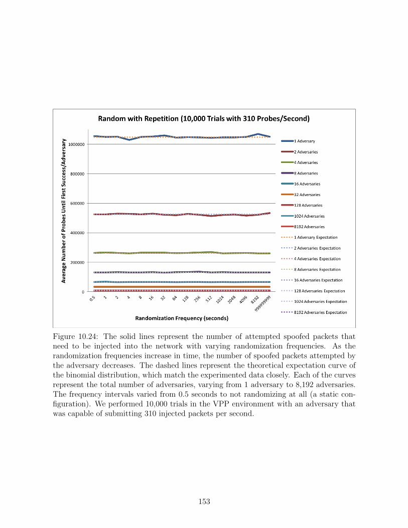
Figure 10.24: The solid lines represent the number of attempted spoofed packets thatneed to be injected into the network with varying randomization frequencies. As therandomization frequencies increase in time, the number of spoofed packets attempted bythe adversary decreases. The dashed lines represent the theoretical expectation curve ofthe binomial distribution, which match the experimented data closely. Each of the curvesrepresent the total number of adversaries, varying from 1 adversary to 8,192 adversaries.The frequency intervals varied from 0.5 seconds to not randomizing at all (a static con-figuration). We performed 10,000 trials in the VPP environment with an adversary thatwas capable of submitting 310 injected packets per second.
153

Figure 10.25: The hypergeometric distribution is followed when the strategy of the ad-versary is to randomly spoof the source and destination IPv6 addresses until a success isobserved without ever repeating previous failed attempts. The results captured experi-mentally match those of the expectation curve when the number of adversaries and thefrequencies at which the defender re-randomizes the network IPv6 addresses are varied.
the IP address configuration changes. Once the randomization intervals increase beyond
256 seconds, the adversary success rates begin to improve more significantly. However,
when there is any amount of randomization frequency beyond 4,096 attempts, the adver-
saries’ success rates become constant. The reason for the constant rate of success beyond
4,096 attempts is because with 20 bits of entropy, the entire attack space can be exhausted
when the adversary is capable of 310 probes per second (310*4,096 ≈ 28 ∗ 212 = 220). The
310 probes per second includes the time to craft, spoof random addresses, and inject the
packet into the network. This strategy follows the hypergeometric distribution which is
overlayed onto the experimental results collected and closely matches those results.
154

The serial guessing strategies shown in Figures 10.26 - 10.27 have similar results as the
random without repetition strategy shown in Figure 10.25. The results of this strat-
egy also follow the hypergeometric distribution and the experimental results are strongly
correlated with that distribution.
10.2.7 Distributed Adversaries
The next set of experiments show the results when the adversary divides the work be-
tween several adversaries to reduce the overall amount of time until success. The number
of distributed adversaries was varied between 2 adversaries and 8,192 adversaries. The
adversaries we evaluated were those that fit the formula 2n where 0 ≤ n ≤ 13. This
experiment setup was developed to evaluate the success rates of a DDoS attack on the
IPv6 randomization scheme within the VPP environment. Each of the curves below the
top curve in Figures 10.25 - 10.27 show the experimental results obtained from a varying
number of adversaries beyond a single adversary.
As the number of adversaries increases, the number of attempts by each adversary de-
creases since the work is divided evenly between them. Similar to the IPv4 results from
the DETERLab experiments shown in Figure 10.5, the y-axis shows the number of probes
required until the first successful spoofed packet is injected into the network by any of the
individual adversaries. The number of probes until a success occurs with two adversaries
present varies between 218 − 219 probes. This is a large number of probes that should
easily be noticed by a defender. As the number of adversaries increases, the number of
overall probes stays the same amongst all adversaries combined but the time needed until
a success occurs is reduced. This reduction in time highlights the need for the defender
to monitor the number of probes observed in the network. As the number of total probes
observed approaches 800,000, at a minimum, the defender should begin to take action on
the noisy activity produced by the adversary. The defender may choose to block the ad-
versaries by activating firewall rules or should at least begin to investigate the anomalous
behavior.
155

Figure 10.26: The hypergeometric distribution is followed when the strategy of the ad-versary is to serially spoof the source and destination IPv6 addresses (starting at IPv6addresses A.B.C.D.E.F.G.0000-T.U.V.W.X.Y.Z.FFFF, where A, B, C, D, E, F, G, T, U,V, W, X, Y, and Z are 16 bit values of an IPv6 address) until success. The results cap-tured experimentally match those of the expectation curve when varying the number ofadversaries and the frequencies at which the defender re-randomizes the IPv6 addresses.
156

Figure 10.27: The hypergeometric distribution is similarly followed when the adversaryfollows the strategy of serially spoofing source and destination IPv6 addresses (starting atIPv6 addresses A.B.C.D.E.F.G.0000-T.U.V.W.X.Y.Z.FFFF, where A, B, C, D, E, F, G,T, U, V, W, X, Y, and Z are 16 bit values of an IPv6 address) until success. The resultscaptured experimentally match those of the expectation curve when varying the numberof adversaries and the frequencies at which the defender re-randomizes the network IPv6addresses.
157
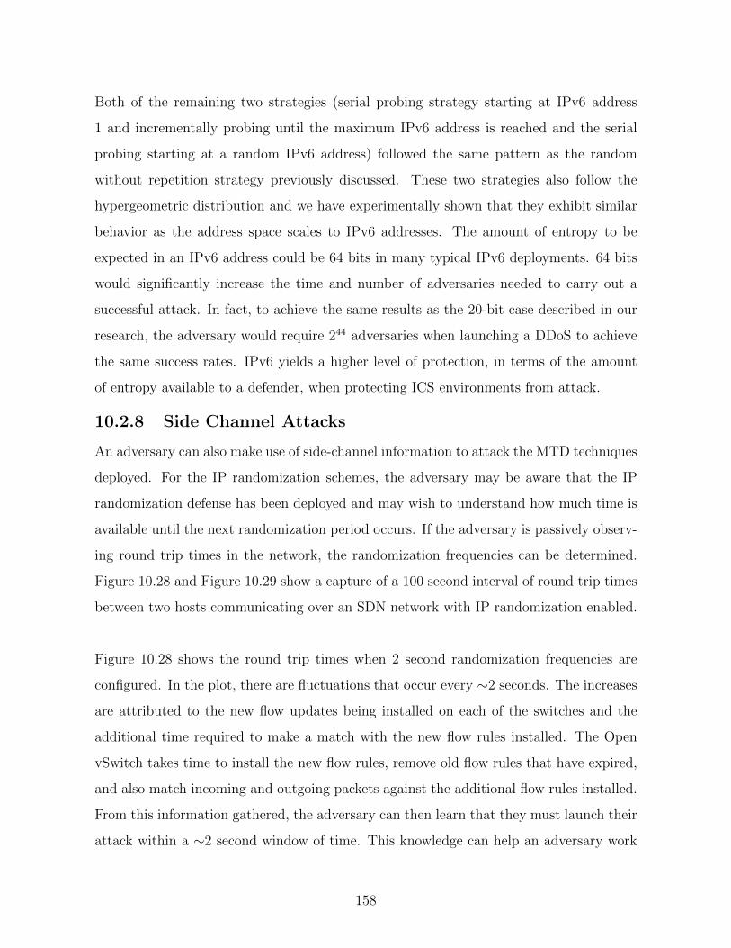
Both of the remaining two strategies (serial probing strategy starting at IPv6 address
1 and incrementally probing until the maximum IPv6 address is reached and the serial
probing starting at a random IPv6 address) followed the same pattern as the random
without repetition strategy previously discussed. These two strategies also follow the
hypergeometric distribution and we have experimentally shown that they exhibit similar
behavior as the address space scales to IPv6 addresses. The amount of entropy to be
expected in an IPv6 address could be 64 bits in many typical IPv6 deployments. 64 bits
would significantly increase the time and number of adversaries needed to carry out a
successful attack. In fact, to achieve the same results as the 20-bit case described in our
research, the adversary would require 244 adversaries when launching a DDoS to achieve
the same success rates. IPv6 yields a higher level of protection, in terms of the amount
of entropy available to a defender, when protecting ICS environments from attack.
10.2.8 Side Channel Attacks
An adversary can also make use of side-channel information to attack the MTD techniques
deployed. For the IP randomization schemes, the adversary may be aware that the IP
randomization defense has been deployed and may wish to understand how much time is
available until the next randomization period occurs. If the adversary is passively observ-
ing round trip times in the network, the randomization frequencies can be determined.
Figure 10.28 and Figure 10.29 show a capture of a 100 second interval of round trip times
between two hosts communicating over an SDN network with IP randomization enabled.
Figure 10.28 shows the round trip times when 2 second randomization frequencies are
configured. In the plot, there are fluctuations that occur every ∼2 seconds. The increases
are attributed to the new flow updates being installed on each of the switches and the
additional time required to make a match with the new flow rules installed. The Open
vSwitch takes time to install the new flow rules, remove old flow rules that have expired,
and also match incoming and outgoing packets against the additional flow rules installed.
From this information gathered, the adversary can then learn that they must launch their
attack within a ∼2 second window of time. This knowledge can help an adversary work
158
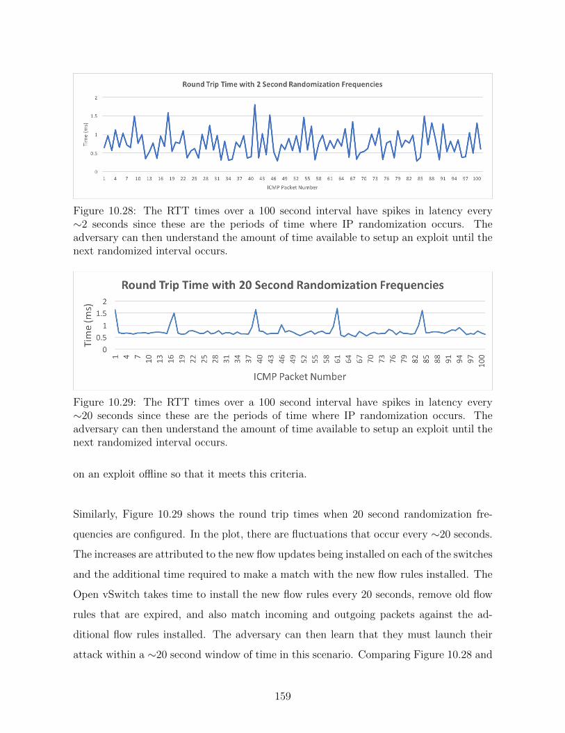
Figure 10.28: The RTT times over a 100 second interval have spikes in latency every∼2 seconds since these are the periods of time where IP randomization occurs. Theadversary can then understand the amount of time available to setup an exploit until thenext randomized interval occurs.
Figure 10.29: The RTT times over a 100 second interval have spikes in latency every∼20 seconds since these are the periods of time where IP randomization occurs. Theadversary can then understand the amount of time available to setup an exploit until thenext randomized interval occurs.
on an exploit offline so that it meets this criteria.
Similarly, Figure 10.29 shows the round trip times when 20 second randomization fre-
quencies are configured. In the plot, there are fluctuations that occur every ∼20 seconds.
The increases are attributed to the new flow updates being installed on each of the switches
and the additional time required to make a match with the new flow rules installed. The
Open vSwitch takes time to install the new flow rules every 20 seconds, remove old flow
rules that are expired, and also match incoming and outgoing packets against the ad-
ditional flow rules installed. The adversary can then learn that they must launch their
attack within a ∼20 second window of time in this scenario. Comparing Figure 10.28 and
159
Figure 10.29 can easily allow the adversary to differentiate the randomization frequencies
of re-randomizing the IPv6 addresses every 2 seconds and every 20 seconds. This knowl-
edge can help an adversary work on an exploit offline so that it meets this criteria.
One possible mitigation for this side channel attack is to configure the randomization
frequency to occur at random frequencies. The random frequencies can be bounded by
user configurable lower and upper bounds to ensure randomization frequencies are occur-
ring often enough to be effective so that the network does not keep the same configuration
for too long. The algorithms to install random flows would have to be slightly modified so
that each randomized flow remains active until the next flow with a different randomly-
chosen expiration time installed. Given that the flows will expire at random times, the
algorithms will have to ensure the next flow is installed before the previous randomized
flow expires. This will require the randomization algorithms to track the previous ran-
domization expiration times and to ensure that the next flows are installed before the
current flow expires.
This is just one example of a side channel attack that an adversary can leverage to their ad-
vantage. Other possible side-channel attacks can include performing power analysis [136]
on the Open vSwitch instances to learn the randomization intervals, or observing the flow
processing time to learn the forwarding table of the Open vSwitch being used [137], or
side-channel attacks on the crypto algorithms to recover keys [138] if a secure communi-
cation channel is used between the controller and the SDN switches. Side channel attacks
should be considered when deploying each of the MTD protections described.
160

Chapter 11
Conclusions
The MTD approaches we developed have been shown to be effective within an ICS en-
vironment. We performed several experiments with a variety of configurations for each
MTD technique. The techniques presented here, although effective individually, are meant
to be a piece of the larger computer security puzzle. The MTD techniques presented here
can be thought of as an additional layer of defense to help protect a system from an ad-
versary attempting to gain an understanding of a system in the early stages of an attack.
Additional defenses can be deployed alongside the MTD techniques to create an even
more secure system. This chapter is meant to highlight the limitations, lessons learned,
opportunities for future research, and to summarize our research.
11.1 Limitations and Lessons Learned
We applied MTD techniques and fault tolerant algorithms to ICS environments with suc-
cessful experimental results. However, there are several lessons learned along the way and
limitations of each approach that we observed. The lessons learned and limitations apply
to both the techniques themselves as well as the experimental processes used to capture
the results. Our intent in this section is to convey that the solutions presented here are ad-
ditional layers of defense available to a defender. Combining the MTD and fault tolerant
techniques with additional security protections is often a requirement in order to meet se-
curity guarantees that are not necessarily provided by the MTD techniques. For example,
the MTD techniques may provide a mitigation to a “hitlist” attack [139], but the MTD
161
techniques themselves do not provide the ability to detect the hitlist attack. Intrusion de-
tection systems (IDSs), firewalls, and virus scanners, for example, should all be included
as part of the overall security protection. The MTD strategies by themselves are not a
security solution that protect against all threats, but rather an additional layer of defense.
One of the lessons learned was that if there are commercially available products that
are under consideration for integration as part of any security solution, they should be
fully evaluated to ensure that they will meet the requirements of the targeted use case.
If there is a mismatch in performance or functionality, early identification is important.
We evaluated several switches that are SDN capable and their implementations varied
significantly. The variations in implementation resulted in drastically different results.
The differences did not impact the feasibility of applying the MTD approaches to an ICS
environment in this case, but could make a difference in environments outside of ICS.
Comparing performance in the software implementation to the hardware implementation
required several experiments to identify and narrow down the observed slow down in la-
tency to be attributed to the software based implementation.
The next lesson learned is that a full analysis of several software options that are candi-
dates for integration into a system should be performed. We leveraged several open source
software packages to support the MTD techniques developed. Open source software can
be an extremely valuable and cost effective solution, but it is not necessarily a stable
production ready solutions. The Open Daylight controller is a large code base written
in the Java programming language with numerous contributors and a large amount of
features available. The complexity of Open Daylight makes it difficult to troubleshoot
and correct any errors encountered. Care should be taken when selecting open source
software as bugs that are discovered along the way may become problematic to correct or
fit within the timeline of the project. We encountered a few OpenDaylight bugs, but we
developed workarounds for those bugs. One problem we observed was when submitting a
bulk amount of flows to be installed contained within a single transaction using a mod-
162

ule named “bulk-o-matic”. When the Open Daylight controller received the bulk flow
inquiries, the bulk-o-matic module would throw several null pointer exceptions frequently
but not every time, even when resubmitting the same query. The workaround was to
continuously submit queries until the bulk-o-matic module accepted the bulk flow query.
This solution was not ideal, but it did work after a few attempted queries so it was not a
major focus of concern. This could be a major concern in a production environment be-
cause there is some uncertainty about when the bulk-o-matic module will actually accept
the bulk flow.
Another lesson learned came from the experimentation process itself where we repeat-
edly performed experiments, each within a higher fidelity environment. Our research
took the approach of running experiments in a simulated environment, then in a virtu-
alized environment, and finally in a representative environment. The reason for this was
that the simulated results provided a means to collect results quickly to evaluate the fea-
sibility of each MTD approach. The virtualized results provided a higher fidelity model
that could be used to collect metrics of each MTD approach. Finally, the representative
environment provided a platform to obtain results that did not potentially overlook pieces
of the system that could not be anticipated in a simulated or virtualized environment. The
sequence of tests provided insights into the effectiveness of each approach and allowed for
cross-validation of each environment. The approach also allowed for easier troubleshoot-
ing early in the process before reaching the representative environment. Not all research
projects will have access to a representative testbed, but in either case it is important
to perform experimentation beforehand to ensure that the technology is feasible before
investing a significant amount of time and money into an approach.
A limitation of the approaches presented are that they each depend on IP routable com-
munications to operate. The concepts can be applied towards communications at layer 2
and below but have not been adapted towards those use cases at this point. The ability
to introduce SDN into ICS environments may also not be an option as the environments
163
may already be fully developed and so it may be difficult to integrate new technologies.
In this scenario, it may be difficult to convince decision makers to upgrade hardware or
introduce software to support the SDN capabilities. This could be a difficult proposition
since standards and requirements must be met before introducing any technology into
an ICS setting. There is also a long testing process that must be satisfied before any
technology can make it to a field deployment, particularly in an ICS setting.
11.2 Future Work
Future areas of research can focus on expanding our research beyond ICS environments.
Additional environments for potential research include cloud computing, Internet of Things
(IoT), and mobile environments, each of which has their own unique sets of constraints
and requirements. The tradeoffs between security and usability can similarly be analyzed
and evaluated in each of those respective environments. Cloud computing has a large
capacity, in terms of resources, however complete control of the physical infrastructure is
lost. The loss of physical control may make some MTD defenses more difficult to deploy
such as the MTD defenses that depend on specific hardware that must be installed. IoT
environments may be difficult to scale path randomization since the enumeration of all
possible paths in the network grows exponentially as the size of the network grows. Mo-
bile environments may make IP randomization more challenging in recognizing the large
number of devices that are dynamically entering and leaving the network constantly.
Furthermore, including the ability to perform forensic analysis as the MTD techniques
are operating is another area of future research. If the IDSs are alarming on packets and
logging randomized IP addresses, that information by itself is of little value to a foren-
sic analyst. The forensic analysis has to be tied into and aware of the MTD techniques
deployed to be effective which needs further investigation. This will be important for
analysis in the event of a system compromise or also when actively observing the current
state of the network. For better situational awareness, the MTD techniques should be
available for security operations personnel to understand the current state of the network.
164

Autonomous systems are another area of future research for each of the MTD techniques
discussed. If the SDN controller fails or one of the SDN capable switches fail, instabilities
within the network will occur. To address this problem, building autonomy into the design
is an interesting area of future research. With autonomy built-in, the SDN controllers and
SDN switches can continue to operate and self-heal after a failure occurs. Currently, fault
tolerant algorithms are developed to protect the SDN controller from failures. However, if
all controllers fail, an interesting area of research is whether or not the switches can detect
the controller failures and continue to operate on their own and take over the role of the
controller. Similarly, if any of the SDN switches fail, an additional area of research would
be to detect such failures and automate the reconfiguration of the network parameters to
continue to operate as expected.
Another area for future research is to investigate the MTD techniques being applied
and retrofitted into environments where SDN is not prevalent. In the case of traditional
networks, an end point solution may be an appropriate area to apply the MTD tech-
niques. As an endpoint solution, however, the MTD techniques should be designed so
that network connections are not broken as network configurations are randomized. For
IP randomization, modifications to the kernel would be necessary to maintain established
connections within the TCP/IP stack during reconfiguration periods. Another solution
outside of the endpoint solution would be to introduce the MTD as a gateway device.
This was the approach taken as part of our research. A related potential area for future
research is to borrow techniques from metamorphic code generation typically used by an
adversary, but instead apply those strategies as a computer defense.
Another area of research is to develop the SDN switches so that they are individually
fault tolerant. Designing in crash tolerant and Byzantine fault tolerant algorithms would
introduce resiliency into the SDN switches. These algorithms would require a cluster con-
figuration for each of the SDN switches which may not be practical in all cases. However,
165

in high fidelity environments, this would create resiliency for both the controller and the
SDN switches. The ability to tolerate faults, crash or Byzantine, is an important area of
research when designing and deploying any security system. An evaluation of the tradeoffs
to the impact on the operational network and the adversary should also be performed in
future areas of research to measure and quantify the effectiveness of the MTD techniques.
11.3 Summary
We have developed several MTD approaches with the goal of introducing additional se-
curity protections to ICS environments. ICS networks are typically statically configured
and have predictable communication patterns over extended periods of time. We have
developed IPv4 randomization, IPv6 randomization, application port number random-
ization, and network communication path to serve as MTD strategies for ICS networks.
We evaluated all of the strategies for their effectiveness within an ICS environment. We
implemented the MTD solutions as an SDN based solution and as an endpoint based
solution. Additionally, we developed the SDN controller systems to be fault tolerant to
system crashes and Byzantine faults.
Each of the MTD strategies proved to be feasible within an ICS setting, all of which
increased latency by less than 50 ms and in most cases under 20 ms. The environments
evaluated as part of our research included a simulated environment, a virtualized environ-
ment and two representative environments. The simulated environment was a standalone
system using local processes to simulate an adversary and a defender. The virtualized
environment consisted of virtual machines to model an ICS system with the same ICS
protocols enabled that would be seen in a field deployment to support the communica-
tions within the network. The representative environments included physical systems that
harnessed the defender systems and the adversary systems.
166

The path randomization technique was the only technique that incurred more than 20 ms
because a much longer path than the fastest optimal path of communication was chosen.
All other approaches were well under the 20 ms requirement of most ICS environments.
The operational measurements captured included bandwidth, throughput, CPU and mem-
ory utilization. Although bandwidth and throughput are typically not critical in most ICS
environments due to the low bandwidth communications, the evaluation was performed
in the event of synchrophasor measurements unit being a part of the network communi-
cations, which can consume bandwidth rates of 150 Mbits/sec[140]. We configured the
network links to 10 Mbits/sec in the experiments performed and there were no significant
performance impacts observed, a ∼1.8% decrease of bandwidth and throughput on aver-
age.
We also captured CPU utilization, memory utilization, and latency metrics when in-
troducing the fault tolerant algorithms. The fault tolerant algorithms included crash
tolerant algorithms and Byzantine fault tolerant algorithms for the SDN controller. The
SDN controller was distributed into a cluster of SDN controllers and was shown to with-
stand crashes and malicious modifications of network flows. The CPU overhead of the
crash tolerant algorithms averaged to be 17.7% more utilization than the baseline. The
Byzantine fault tolerant algorithms consumed 17.9% of the CPU to operate. These met-
rics may or may not be acceptable depending on the load placed on the SDN controller
which would vary in each deployment. The memory requirements on the controller were
quite a bit higher, mainly attributed to the open source SDN controller operating in a
Java Virtual Machine that required 512 MB to run. An additional 92.2% and 92.6%
memory was utilized when enabling the Paxos crash tolerant algorithms and the Byzan-
tine fault tolerant algorithms, respectably. The latency improved when enabling the SDN
network because packets match criteria was minimal and ARP requests were not needed.
The baseline round-trip time was observed to be 0.612 ms, while the crash tolerant and
Byzantine tolerant algorithms showed a round-trip time of 0.546 ms and 0.542 ms, respec-
tively. The fault tolerant algorithms impact observed in the set of experiments performed
167

as part of our research was not a factor.
We evaluated several SDN capable switches, including two hardware switches and one
software switch. The two hardware switches varied in their functionality. The first switch
performed the match criteria and the action for the flows within software. The second
switch performed these same operations in hardware. The latency was drastically reduced
in the hardware implementation compared to the software implementation. The delays
of the hardware switch were in the microseconds, while the software flow implementation
gave results that were delayed within the milliseconds. The open source software switch
evaluated also gave results that were in the milliseconds of increased delay. All SDN
capable switches were well within the constraints of a typical ICS environment, but the
hardware switch had the best performance results observed.
MTD is an active and promising area of research for ICS environments. We have shown
that MTD techniques can be beneficial and effective in such a setting. The approaches
were researched and analyzed against a number of adversaries either performing a DoS
or DDoS attack. We performed experiments that showed that the amount of entropy
available to the defender directly affected the adversaries’ success rates. As the entropy
increased, the success rates of the adversary decreased. We also considered adversaries per-
forming side channel attacks and we discussed strategies to prevent such attacks against
the MTD techniques. We then evaluated the operational costs and adversarial costs
against one another to determine a balance between security and usability.
The MTD approaches presented here are meant to provide an additional layer of defense
to an ICS system. The MTD approaches are not intended to be deployed by themselves,
but integrated into a system of security tools to achieve an elevated overall level of se-
curity. A number of open problems that can build upon our research include evaluating
these approaches in environments outside of ICS, exploring possible options of developing
the same techniques for systems that have not adopted SDN, integrating the MTD ap-
168

proaches within existing security monitoring systems, developing the MTD solutions so
that they can run autonomously if needed, introducing fault tolerant algorithms to the
SDN switches, and finally adding in self-healing techniques to recover from attacks that
are successful. Each of the future areas of research can improve the existing concepts
and create more resilient solutions that complement and build upon our research. We
have shown that MTD techniques can be successful in an ICS setting and they have the
potential of being applied more broadly towards general computing environments.
169

References
[1] Diego Ongaro and John K. Ousterhout, “In Search of an Understandable Consensus
Algorithm,” in USENIX Annual Technical Conference, pp. 305–319, 2014.
[2] Keith Stouffer, Joe Falco, and Karen Scarfone, “Guide to Industrial Control Systems
(ICS) Security,” NIST special publication, vol. 800, no. 82, pp. 16–16, 2011.
[3] Rodrigo Chandia, Jesus Gonzalez, Tim Kilpatrick, Mauricio Papa, and Sujeet
Shenoi, “Security Strategies for SCADA Networks,” in Critical Infrastructure Pro-
tection, pp. 117–131, Springer, 2007.
[4] Alvaro A. Cardenas, Saurabh Amin, Zong-Syun Lin, Yu-Lun Huang, Chi-Yen
Huang, and Shankar Sastry, “Attacks Against Process Control Systems: Risk As-
sessment, Detection, and Response,” in Proceedings of the 6th ACM symposium on
information, computer and communications security, pp. 355–366, ACM, 2011.
[5] Yu-Lun Huang, Alvaro A. Cardenas, Saurabh Amin, Zong-Syun Lin, Hsin-Yi Tsai,
and Shankar Sastry, “Understanding the Physical and Economic Consequences of
Attacks on Control Systems,” International Journal of Critical Infrastructure Pro-
tection, vol. 2, no. 3, pp. 73–83, 2009.
[6] Bill Miller and Dale Rowe, “A Survey SCADA of and Critical Infrastructure In-
cidents,” in Proceedings of the 1st Annual conference on Research in information
technology, pp. 51–56, ACM, 2012.
[7] Nicolas Falliere, Liam O. Murchu, and Eric Chien, “W32. Stuxnet Dossier,” White
paper, Symantec Corp., Security Response, vol. 5, 2011.
[8] Pouyan Pourbeik, Prabha S. Kundur, and Carson W. Taylor, “The Anatomy of a
Power Grid Blackout,” IEEE Power and Energy Magazine, vol. 4, no. 5, pp. 22–29,
2006.
170
[9] Gaoqi Liang, Steven Weller, Junhua Zhao, Fengji Luo, and Zhao .Y. Dong, “The
2015 Ukraine Blackout: Implications for False Data Injection Attacks,” IEEE Trans-
actions on Power Systems, vol. 32, pp. 3317–3318, July 2017.
[10] Siddharth Sridhar and Manimaran Govindarasu, “Data Integrity Attacks and Their
Impacts on SCADA Control system,” in IEEE PES General Meeting, pp. 1–6, July
2010.
[11] Hassan Farhangi, “The Path of the Smart Grid,” Power and energy magazine,
IEEE, vol. 8, no. 1, pp. 18–28, 2010.
[12] Rosslin John Robles, Min-kyu Choi, Eun-suk Cho, Seok-soo Kim, Gil-cheol Park,
and Jang-Hee Lee, “Common Threats and Vulnerabilities of Critical Infrastruc-
tures,” International journal of control and automation, vol. 1, no. 1, pp. 17–22,
2008.
[13] Carl H. Hauser, David E. Bakken, and Anjan Bose, “A Failure to Communicate:
Next Generation Communication Requirements, Technologies, and Architecture for
the Electric Power Grid,” IEEE Power and Energy Magazine, vol. 3, no. 2, pp. 47–
55, 2005.
[14] Ragunathan Rajkumar, Insup Lee, Lui Sha and John Stankovic, “Cyber-Physical
Systems: The Next Computing Revolution,” in Design Automation Conference,
pp. 731–736, June 2010.
[15] Goran N. Ericsson, “Cyber Security and Power System CommunicationEssential
Parts of a Smart Grid Infrastructure,” IEEE Transactions on Power Delivery,
vol. 25, no. 3, pp. 1501–1507, 2010.
[16] Sushil Jajodia, Anup K. Ghosh, V.S. Subrahmanian, Vipin Swarup, Cliff Wang,
and X. Sean Wang, Moving Target Defense II. Springer, 2013.
171

[17] Byungho Min, Vijay Varadharajan, Udaya Tupakula, and Michael Hitchens, “An-
tivirus Security: Naked During Updates,” Software: Practice and Experience,
vol. 44, no. 10, pp. 1201–1222, 2014.
[18] Feng Xue, “Attacking Antivirus,” in Black Hat Europe Conference, 2008.
[19] Steven A. Hofmeyr and Stephanie Forrest, “Architecture for an Artificial Immune
System,” Evolutionary Computation, vol. 8, no. 4, pp. 443–473, 2000.
[20] Ehab Al-Shaer, Qi Duan, Jafar Haadi Jafarian, “Random Host Mutation for Moving
Target Defense,” in SecureComm, pp. 310–327, Springer, 2012.
[21] Spyros Antonatos, Periklis Akritidis, Evangelos P. Markatos, and Kostas G. Anag-
nostakis, “Defending Against Hitlist Worms Using Network Address Space Ran-
domization,” Computer Networks, vol. 51, no. 12, pp. 3471 – 3490, 2007.
[22] Azulai Sharon, Ran Levy, Yaacov Cohen, Alexander Haiut, Ariel Stroh, David Raz,
“Automatic Network Traffic Analysis,” Oct. 24 2000. US Patent 6,137,782.
[23] Lucas F. Muller, Rodrigo R. Oliveira, Marcelo C. Luizelli, Luciano P. Gaspary,
and Marinho P. Barcellos, “Survivor: An Enhanced Controller Placement Strategy
for Improving SDN Survivability,” in Global Communications Conference (GLOBE-
COM), 2014 IEEE, pp. 1909–1915, IEEE, 2014.
[24] David Goldschlag, Michael Reed, and Paul Syverson, “Onion Routing for Anony-
mous and Private Internet Connections,” Communications of the ACM, vol. 42,
no. 2, pp. 39–41, 1999.
[25] Vitaly Shmatikov and Ming-Hsiu Wang, “Timing Analysis in Low-Latency Mix
Networks: Attacks and Defenses,” Computer Security–ESORICS 2006, pp. 18–33,
2006.
[26] Jean-Francois Raymond, “Traffic Analysis: Protocols, Attacks, Design Issues
and Open Problems,” in Designing Privacy Enhancing Technologies, pp. 10–29,
Springer, 2001.
172

[27] Roger Dingledine, Nick Mathewson, and Paul Syverson, “Tor: The Second-
Generation Onion Router,” in Usenix Security, 2004.
[28] , “The Tor Project.” https://metrics.torproject.org/torperf.html, 2014.
[29] Sambuddho Chakravarty, Marco V. Barbera, Georgios Portokalidis, Michalis Poly-
chronakis, and Angeles D. Keromytis, “On the Effectiveness of Traffic Analysis
Against Anonymity Networks Using Flow Records,” in PAM, pp. 247–257, Springer,
2014.
[30] Gildas Nya Tchabe and Yinhua Xu, “Anonymous Communications: A Survey on
I2P,” CDC Publication Theoretische Informatik-Kryptographie und Computeralge-
bra (https://www. cdc. informatik. tu-darmstadt. de), 2014.
[31] Angelos D. Keromytis, Vishal Misra, and Dan Rubenstein, “SOS: An Architecture
For Mitigating DDoS Attacks,” IEEE Journal of Selected Areas in Communications,
vol. 22, no. 1, pp. 176–188, 2004.
[32] Kamran Ahsan and Deepa Kundur, “Practical Data Hiding in TCP/IP,” in Proc.
Workshop on Multimedia Security at ACM Multimedia, vol. 2, 2002.
[33] Lexi Pimenidis and Tobias Kolsch, “Transparent Anonymization of IP Based Net-
work Traffic,” In Proceedings of 10th Nordic Workshop on Secure IT-Systems, 2005.
[34] H. Okhravi, M. A. Rabe, T. J. Mayberry, W. G. Leonard, T. R. Hobson, D. Bigelow,
and W. W. Streilein, “Survey of Cyber Moving Target Techniques,” tech. rep.,
MASSACHUSETTS INST OF TECH LEXINGTON LINCOLN LAB, 2013.
[35] Babak Salamat, Todd Jackson, Gregor Wagner, Christian Wimmer, and Michael
Franz, “Runtime Defense Against Code Injection Attacks Using Replicated Exe-
cution,” IEEE Transactions on Dependable and Secure Computing, vol. 8, no. 4,
pp. 588–601, 2011.
173

[36] David A. Holland, Ada T. Lim, and Margo I. Seltzer, “An Architecture a Day Keeps
the Hacker Away,” ACM SIGARCH Computer Architecture News, vol. 33, no. 1,
pp. 34–41, 2005.
[37] Hamed Okhravi, Adam Comella, Eric Robinson, and Joshua Haines, “Creating a
Cyber Moving Target for Critical Infrastructure Applications Using Platform Di-
versity,” International Journal of Critical Infrastructure Protection, vol. 5, no. 1,
pp. 30–39, 2012.
[38] Benjamin Cox, David Evans, Adrian Filipi, Jonathan Rowanhill, Wei Hu, Jack
Davidson, John Knight, Anh Nguyen-Tuong, and Jason Hiser, “N-Variant Systems:
A Secretless Framework for Security Through Diversity,” in USENIX Security Sym-
posium, pp. 105–120, 2006.
[39] McLaughlin, Stephen E and Podkuiko, Dmitry and Delozier, Adam and Mi-
adzvezhanka, Sergei and McDaniel, Patrick, “Embedded Firmware Diversity for
Smart Electric Meters,” in HotSec, 2010.
[40] Gaurav S . Kc, Angelos D. Keromytis, and Vassilis Prevelakis, “Countering Code-
Injection Attacks with Instruction-Set Randomization,” in Proceedings of the 10th
ACM conference on Computer and communications security, pp. 272–280, ACM,
2003.
[41] Hovav Shacham, Matthew Page, Ben Pfaff, Eu-Jin Goh, Nagendra Modadugu, and
Dan Boneh, “On the Effectiveness of Address-Space Randomization,” in Proceedings
of the 11th ACM conference on Computer and communications security, pp. 298–
307, ACM, 2004.
[42] Ana Nora Sovarel, David Evans, and Nathanael Paul, “Where’s the FEEB? The
Effectiveness of Instruction Set Randomization,” in USENIX Security Symposium,
2005.
[43] Jonathan Ganz and Sean Peisert, “ASLR: How Robust is the Randomness?,” in
Proceedings of the 2017 IEEE Secure Development Conference (SecDev), 2017.
174

[44] Stephanie Forrest, Anil Somayaji, and David H. Ackley, “Building Diverse Com-
puter Systems,” in Operating Systems, 1997., The Sixth Workshop on Hot Topics
in, pp. 67–72, IEEE, 1997.
[45] Cristian Cadar, Periklis Akritidis, Manuel Costa, Jean-Phillipe Martin, and Miguel
Castro, “Data Randomization,” tech. rep., Technical Report TR-2008-120, Mi-
crosoft Research, 2008. Cited on, 2008.
[46] Stephen W. Boyd, and Angelos D. Keromytis, “SQLrand: Preventing SQL Injection
Attacks,” in Applied Cryptography and Network Security, pp. 292–302, Springer,
2004.
[47] Adam J. O’Donnell, and Harish Sethu, “On Achieving Software Diversity for Im-
proved Network Security using Distributed Coloring Algorithms,” in Proceedings of
the 11th ACM conference on Computer and communications security, pp. 121–131,
ACM, 2004.
[48] Qinghua Zhang and Douglas S. Reeves, “Metaaware: Identifying Metamorphic Mal-
ware,” in Computer Security Applications Conference, 2007. ACSAC 2007. Twenty-
Third Annual, pp. 411–420, IEEE, 2007.
[49] Melanie R. Rieback, Bruno Crispo, and Andrew S. Tanenbaum, “Is Your Cat In-
fected with a Computer Virus?,” in Pervasive Computing and Communications,
2006. PerCom 2006. Fourth Annual IEEE International Conference on, pp. 10–pp,
IEEE, 2006.
[50] Ilsun You and Kangbin Yim, “Malware Obfuscation Techniques: A Brief Survey,”
in 2010 International conference on broadband, wireless computing, communication
and applications, pp. 297–300, IEEE, 2010.
[51] J. Adam Butts and Guri Sohi, “Dynamic Dead-Instruction Detection and Elim-
ination,” ACM SIGOPS Operating Systems Review, vol. 36, no. 5, pp. 199–210,
2002.
175

[52] Andrew H. Sung, Jianyun Xu, Patrick Chavez, and Srinivas Mukkamala, “Static
Analyzer of Vicious Executables (save),” in Computer Security Applications Con-
ference, 2004. 20th Annual, pp. 326–334, IEEE, 2004.
[53] Babak Salamat, Andreas Gal, and Michael Franz, “Reverse Stack Execution in a
Multi-Variant Execution Environment,” in Workshop on Compiler and Architectural
Techniques for Application Reliability and Security, pp. 1–7, 2008.
[54] Bjorn De Sutter, Bertrand Anckaert, Jens Geiregat, Dominique Chanet, and Koen
De Bosschere, “Instruction Set Limitation in Support of Software Diversity,” in
Information security and cryptology–ICISC 2008, pp. 152–165, Springer, 2009.
[55] David J. Kuck, Robert H. Kuhn, David A. Padua, and Bruce Leasure, and Michael
Wolfe, “Dependence Graphs and Compiler Optimizations,” in Proceedings of the
8th ACM SIGPLAN-SIGACT symposium on Principles of programming languages,
pp. 207–218, ACM, 1981.
[56] Rui Zhuang, Su Zhang, Scott A DeLoach, Xinming Ou, and Anoop Singhal,
“Simulation-based Approaches to Studying Effectiveness of Moving-Target Network
Defense,” in National Symposium on Moving Target Research, pp. 1–12, 2012.
[57] Luigi Atzori, Antonio Iera, and Giacomo Morabito, “The Internet of Things: A
Survey,” Computer networks, vol. 54, no. 15, pp. 2787–2805, 2010.
[58] Harald Sundmaeker, Patrick Guillemin, Peter Friess, and Sylvie Woelffle, “Vision
and Challenges for Realising the Internet of Things,” Cluster of European Research
Projects on the Internet of Things, European Commision, vol. 3, no. 3, pp. 34–36,
2010.
[59] Sean Dieter Tebje Kelly, Nagender Kumar Suryadevara, and Subhas Chandra
Mukhopadhyay, “Towards the Implementation of IoT for Environmental Condi-
tion Monitoring in Homes,” IEEE Sensors Journal, vol. 13, no. 10, pp. 3846–3853,
2013.
176

[60] Rui Zhuang, Scott A. DeLoach, and Xinming Ou, “Towards a Theory of Moving
Target Defense,” in Proceedings of the First ACM Workshop on Moving Target
Defense, pp. 31–40, ACM, 2014.
[61] North American Electricity Council, “NERC Critical Infrastructure Pro-
tection (CIP) Reliability Standards.” http://www.nerc.com/pa/Stand/Pages/
CIPStandards.aspx, 2009.
[62] Georg Disterer, “ISO/IEC 27000, 27001 and 27002 for Information Security Man-
agement,” Journal of Information Security, vol. 4, no. 02, p. 92, 2013.
[63] North American Electric Reliability Corporation, “North American Electric Relia-
bility Corporation (NIST) Cybersecurity Framework (CSF).” https://www.nist.
gov/cyberframework, 2014.
[64] Kristina Hamachi LaCommare and Joseph H. Eto, “Cost of Power Interruptions
to Electricity Consumers in the United States (U.S.),” Energy, vol. 31, no. 12,
pp. 1845–1855, 2006.
[65] Goran Andersson, Peter Donalek, Richard Farmer, Nikos Hatziargyriou, Innocent
Kamwa, Prabhashankar Kundur, Nelson Martins, John Paserba, Pouyan Pourbeik,
and Juan Sanchez-Gasca, Ronald Shultz, John A. Stankovic, Carson Taylor, and
Vijay Vittal, “Causes of the 2003 Major Grid Blackouts in North America and Eu-
rope, and Recommended Means to improve System Dynamic Performance,” IEEE
Transactions on Power Systems, vol. 20, no. 4, pp. 1922–1928, 2005.
[66] U.S.-Canada Power System Outage Task Force, “Final Report on the August 14,
2003 Blackout in the United States and Canada: Causes and Recommendations,”
IEEE Transactions on Power Systems, vol. 20, no. 4, pp. 1922–1928, 2005.
[67] G. Brooke Anderson and Michelle L. Bell, “Lights Out: Impact of the August 2003
Power Outage on Mortality in New York, NY,” Epidemiology (Cambridge, Mass.),
vol. 23, no. 2, p. 189, 2012.
177
[68] IDA Modbus, “Modbus Application Protocol Specification v1. 1a,” North Grafton,
Massachusetts (www. modbus. org/specs. php), 2004.
[69] Gordon R. Clarke, Deon Reynders, and Edwin Wright, Practical Modern SCADA
Protocols: DNP3, 60870.5 and Related Systems. Newnes, 2004.
[70] Feld, Joachim, “PROFINET-Scalable Factory Communication for all Applications,”
in Factory Communication Systems, 2004. Proceedings. 2004 IEEE International
Workshop on, pp. 33–38, IEEE, 2004.
[71] Riley Walters, “Cyber Attacks on U.S. Companies in 2014,” The Heritage Founda-
tion, vol. 4289, pp. 1–5, 2014.
[72] Bonnie Zhu, Anthony Joseph, and Shankar Sastry, “A Taxonomy of Cyber Attacks
on SCADA Systems,” in Internet of things (iThings/CPSCom), 2011 international
conference on and 4th international conference on cyber, physical and social com-
puting, pp. 380–388, IEEE, 2011.
[73] Frederic P. Miller, Agnes F. Vandome, and John McBrewster, “Advanced Encryp-
tion Standard,” 2009.
[74] Pawel R. Chodowiec, Comparison of the Hardware Performance of the AES Candi-
dates using Reconfigurable Hardware. PhD thesis, George Mason University, 2002.
[75] F. Russell Robertson, J. Ritchie Carroll, William Sanders, Timothy Yardley, Erich
Heine, Mark Hadley, David McKinnon, Barbara Motteler, Jay Giri, William Walker,
and Esrick McCartha, “Secure Information Exchange Gateway for Electric Grid
Operations,” tech. rep., Grid Protection Alliance, Chattanooga, TN (United States),
2014.
[76] Steven A. Hurd, Jason E. Stamp, and Adrian R. Chavez, “OPSAID Initial Design
and Testing Report,” Department of Energy, 2007.
178

[77] Brian P. Smith, and John Stewart, Ron Halbgewachs, and Adrian Chavez, “Cyber
Security Interoperability-The Lemnos Project,” in 53rd ISA POWID Symposium,
vol. 483, pp. 50–59, 2010.
[78] Ronald D. Halbgewachs and Adrian R. Chavez, “OPSAID Improvements and Ca-
pabilities Report,” tech. rep., Sandia National Laboratories, 2011.
[79] Thomas Parke Hughes, Networks of Power: Electrification in Western Society,
1880-1930. JHU Press, 1993.
[80] Paolo Castello, Paolo Ferrari, Alessandra Flammini, Alessandra Muscas, and Ste-
fano Rinaldi, “An IEC 61850-Compliant Distributed PMU for Electrical Substa-
tions,” in Applied Measurements for Power Systems (AMPS), 2012 IEEE Interna-
tional Workshop on, pp. 1–6, IEEE, 2012.
[81] Federico Milano and Marian Anghel, “Impact of Time Delays on Power System
Stability,” IEEE Transactions on Circuits and Systems I: Regular Papers, vol. 59,
no. 4, pp. 889–900, 2012.
[82] R. E. Mackiewicz, “Overview of IEC 61850 and Benefits,” in Power Systems Con-
ference and Exposition, 2006. PSCE’06. 2006 IEEE PES, pp. 623–630, IEEE, 2006.
[83] Halsall, Fred and Links, Data, “Computer networks and open systems,” Addison-
Wesley Publishers, pp. 112–125, 1995.
[84] Dorothy Elizabeth Robling Denning, Information Warfare and Security, vol. 4.
Addison-Wesley Reading, MA, 1999.
[85] Srikanth Kandula, Dina Katabi, Matthias Jacob, and Arthur Berger, “Botz-4-Sale:
Surviving Organized DDoS Attacks that Mimic Flash Crowds,” in Proceedings of
the 2nd conference on Symposium on Networked Systems Design & Implementation-
Volume 2, pp. 287–300, USENIX Association, 2005.
179
[86] Jelena Mirkovic and Peter Reiher, “A Taxonomy of DDoS Attack and DDoS Defense
Mechanisms,” ACM SIGCOMM Computer Communication Review, vol. 34, no. 2,
pp. 39–53, 2004.
[87] Rohan M. Egelman, Cormac Herley, and Paul C. Van Oorschot, “Markets for Zero-
Day Exploits: Ethics and Implications,” in Proceedings of the 2013 workshop on
New security paradigms workshop, pp. 41–46, ACM, 2013.
[88] Christian Gronroos, “Service Quality: The Six Criteria of Good Perceived Service,”
Review of business, vol. 9, no. 3, p. 10, 1988.
[89] Wes Sonnenreich, Jason Albanese, and Bruce Stout, “Return On Security Invest-
ment (ROSI)-A Practical Quantitative Model,” Journal of Research and practice in
Information Technology, vol. 38, no. 1, pp. 45–56, 2006.
[90] Peter Mell and Tim Grance, “The NIST Definition of Cloud Computing,” NIST
Special Publication, vol. 800, p. 145, 2011.
[91] Paul G. Dorey and Armando Leite, “Commentary: Cloud Computing–A Security
Problem or Solution?,” information security technical report, vol. 16, no. 3, pp. 89–
96, 2011.
[92] Elena Gabriela Barrantes, David H. Ackley, Trek S. Palmer, Darko Stefanovic, and
Dino Dai Zovi, “Randomized Instruction Set Emulation to Disrupt Binary Code
Injection Attacks,” in Proceedings of the 10th ACM conference on Computer and
communications security, pp. 281–289, ACM, 2003.
[93] Per Larsen, Andrei Homescu, Stefan Brunthaler, and Michael Franz, “SoK: Auto-
mated Software Diversity,” in Security and Privacy (SP), 2014 IEEE Symposium
on, pp. 276–291, IEEE, 2014.
[94] Nicholas Carlini and David Wagner, “ROP is Still Dangerous: Breaking Modern
Defenses,” in USENIX Security Symposium, pp. 385–399, 2014.
180

[95] Council, Industry Advisory, “Federal risk and authorization management program
(FedRAMP),” 2012.
[96] Michael Larsen, and Fernando Gont, “Recommendations for Transport-Protocol
Port Randomization,” tech. rep., 2011.
[97] Rogerio Leao Santos de Oliveira, Ailton Akira Shinoda, Christiane Marie Schweitzer,
and Ligia Rodrigues Prete, “Using Mininet for Emulation and Prototyping Software-
Defined Networks,” in Communications and Computing (COLCOM), 2014 IEEE
Colombian Conference on, pp. 1–6, IEEE, 2014.
[98] Jan Medved, Robert Varga, Anton Tkacik, and Ken Gray, “Opendaylight: Towards
a Model-Driven SDN Controller Architecture,” in 2014 IEEE 15th International
Symposium on, pp. 1–6, IEEE, 2014.
[99] Nick McKeown, Tom Anderson, Hari Balakrishnan, Guru Parulkar, Larry Peterson,
Jennifer Rexford, Scott Shenker, and Jonathan Turner, “OpenFlow: Enabling Inno-
vation in Campus Networks,” ACM SIGCOMM Computer Communication Review,
vol. 38, no. 2, pp. 69–74, 2008.
[100] Yakov Rekhter, Bob Moskowitz, Daniel Karrenberg, Geert Jan de Groot, and Eliot
Lear, “Address Allocation for Private Internets,” tech. rep., 1996.
[101] Alexander Shalimov, Dmitry Zuikov, Daria Zimarina, Vasily Pashkov, and Ruslan
Smeliansky, “Advanced Study of SDN/OpenFlow Controllers,” in Proceedings of
the 9th central & eastern european software engineering conference in russia, p. 1,
ACM, 2013.
[102] Douglas Brent West, Introduction to Graph Theory, vol. 2. Prentice hall Upper
Saddle River, 2001.
[103] Mogens Blanke, Michel Kinnaert, Jan Lunze, Marcel Staroswiecki, and J. Schroder,
Diagnosis and Fault-Tolerant Control, vol. 691. Springer, 2006.
181
[104] Leslie Lamport, “Using Time Instead of Timeout for Fault-Tolerant Distributed
Systems,” ACM Transactions on Programming Languages and Systems (TOPLAS),
vol. 6, no. 2, pp. 254–280, 1984.
[105] Miguel Castro and Barbara Liskov, “Practical Byzantine Fault Tolerance,” in OSDI,
vol. 99, pp. 173–186, 1999.
[106] Jim Gray, “A Transaction Model,” Automata, Languages and Programming,
pp. 282–298, 1980.
[107] Dale Skeen, “Nonblocking Commit Protocols,” in Proceedings of the 1981 ACM
SIGMOD international conference on Management of data, pp. 133–142, ACM,
1981.
[108] Biswanath Mukherjee, L. Todd Heberlein, and Karl N. Levitt, “Network Intrusion
Detection,” IEEE network, vol. 8, no. 3, pp. 26–41, 1994.
[109] Leslie Lamport, “Paxos Made Simple,” ACM Sigact News, vol. 32, no. 4, pp. 18–25,
2001.
[110] Patrick Hunt, Mahadev Konar, Flavio Paiva Junqueira, and Benjamin Reed,
“ZooKeeper: Wait-Free Coordination for Internet-Scale Systems,” in USENIX an-
nual technical conference, vol. 8, p. 9, Boston, MA, USA, 2010.
[111] Tushar D. Chandra, Robert Griesemer, and Joshua Redstone, “Paxos Made Live:
An Engineering Perspective,” in Proceedings of the twenty-sixth annual ACM sym-
posium on Principles of distributed computing, pp. 398–407, ACM, 2007.
[112] Lisa Glendenning, Ivan Beschastnikh, Arvind Krishnamurthy, and Thomas Ander-
son, “Scalable Consistency in Scatter,” in Proceedings of the Twenty-Third ACM
Symposium on Operating Systems Principles, pp. 15–28, ACM, 2011.
[113] Leslie Lamport and Robert Shostak and Marshall Pease, “The Byzantine Generals
Problem,” ACM Transactions on Programming Languages and Systems (TOPLAS),
vol. 4, pp. 382–401, July 1982.
182

[114] Miguel Castro and Barbara Liskov, “Practical Byzantine Fault Tolerance and Proac-
tive Recovery,” ACM Transactions on Computer Systems (TOCS), vol. 20, pp. 398–
461, Nov. 2002.
[115] Yilei Zhang, Zibin Zheng, and Michael R. Lyu, “BFTCloud: A Byzantine Fault Tol-
erance Framework for Voluntary-Resource Cloud Computing,” in Cloud Computing
(CLOUD), 2011 IEEE International Conference on, pp. 444–451, IEEE, 2011.
[116] Sisi Duan and Sean Peisert and Karl Levitt, “hBFT: Fast Byzantine Fault Tol-
erance With Optimal Resilience,” IEEE Transactions on Dependable and Secure
Computing (TDSC), vol. 12, pp. 58–70, Jan./Feb. 2015.
[117] James Cowling, Daniel Myers, Barbara Liskov, Rodrigo Rodrigues, and Liuba
Shrira, “HQ Replication: A Hybrid Quorum Protocol for Byzantine Fault Toler-
ance,” in Proceedings of the 7th symposium on Operating systems design and imple-
mentation, pp. 177–190, USENIX Association, 2006.
[118] Ramakrishna Kotla, Lorenzo Alvisi, Allen Dahlin, Allen Clement and Edmund
Wong, “Zyzzyva: Speculative Byzantine Fault Tolerance,” in ACM SIGOPS Oper-
ating Systems Review, vol. 41, pp. 45–58, ACM, 2007.
[119] Sean Whalen, “An Introduction to ARP Spoofing,” Node99 [Online Document],
April, 2001.
[120] Adam Kieyzun, Philip J. Guo, Karthick Jayaraman, and Michael D. Ernst, “Au-
tomatic Creation of SQL Injection and Cross-Site Scripting Attacks,” in Software
Engineering, 2009. ICSE 2009. IEEE 31st International Conference on, pp. 199–
209.
[121] Sisi Duan and Hein Meling and Sean Peisert and Haibin Zhang, “BChain: Byzan-
tine Replication with High Throughput and Embedded Reconfiguration,” in Pro-
ceedings of the 18th International Conference on Principles of Distributed Systems
(OPODIS), (Cortina, Italy), Dec. 15–19, 2014.
183
[122] Teerawat Issariyakul and Ekram Hossain, Introduction to Network Simulator NS2.
Springer Science & Business Media, 2011.
[123] Michael Mirkovic and Terry Benzel, “Teaching Cybersecurity with DeterLab,” IEEE
Security & Privacy, vol. 10, no. 1, pp. 73–76, 2012.
[124] Norman L. Johnson, Adrienne W. Kemp, and Samuel Kotz, Univariate Discrete
Distributions, vol. 444. John Wiley & Sons, 2005.
[125] J.G. Skellam, “A Probability Distribution Derived from the Binomial Distribution
by Regarding the Probability of Success as Variable Between the Sets of Trials,”
Journal of the Royal Statistical Society. Series B (Methodological), vol. 10, no. 2,
pp. 257–261, 1948.
[126] Gregor N. Purdy, Linux iptables Pocket Reference: Firewalls, NAT & Accounting.
“O’Reilly Media, Inc.”, 2004.
[127] Steven M. Rinaldi, James P. Peerenboom, and Terrence K. Kelly, “Identifying,
Understanding, and Analyzing Critical Infrastructure Interdependencies,” Control
Systems, IEEE, vol. 21, no. 6, pp. 11–25, 2001.
[128] Stuart Russell and Peter Norvig, “A Modern Approach,” Artificial Intelligence.
Prentice-Hall, Egnlewood Cliffs, vol. 25, p. 27, 1995.
[129] J. Johnson, “Virtual Power Plants and Large Scale Renewable Integration,” tech.
rep.
[130] Alysson Bessani, Joao Sousa, and Eduardo E.P. Alchieri, “State Machine Repli-
cation for the Masses with BFT-SMaRt,” in Dependable Systems and Networks
(DSN), 2014 44th Annual IEEE/IFIP International Conference on, pp. 355–362,
IEEE, 2014.
[131] Kannan Govindarajan, Kong Chee Meng, Hong Ong, Wong Ming Tat, Sridhar
Sivanand, and Low Swee Leong, “Realizing the Quality of Service (QoS) in Software-
184

Defined Networking (SDN) based Cloud Infrastructure,” in Information and Com-
munication Technology (ICoICT), 2014 2nd International Conference on, pp. 505–
510, IEEE, 2014.
[132] Eric Rescorla, SSL and TLS: Designing and Building Secure Systems, vol. 1.
Addison-Wesley Reading, 2001.
[133] Tyson Macaulay and Bryan L. Singer, Cybersecurity for Industrial Control Systems:
SCADA, DCS, PLC, HMI, and SIS. CRC Press, 2011.
[134] Stephen E. Deering, “Internet Protocol, Version 6 (IPv6) Specification,” 1998.
[135] Susan Thomson, “IPv6 Stateless Address Autoconfiguration,” 1998.
[136] Stefan Mangard, Elisabeth Oswald, and Thomas Popp, Power Analysis Attacks:
Revealing the Secrets of Smart Cards, vol. 31. Springer Science & Business Media,
2008.
[137] Adnan Akhunzada, Ejaz Ahmed, Abdullah Gani, Muhammad Khurram Khan,
Muhammad Imran, and Sghaier Guizani, “Securing Software Defined Networks:
Taxonomy, Requirements, and Open Issues,” IEEE Communications Magazine,
vol. 53, no. 4, pp. 36–44, 2015.
[138] Mathieu Renauld, Francois-Xavier Standaert, and Nicolas Veyrat-Charvillon, “Al-
gebraic Side-Channel Attacks on the AES: Why Time also Matters in DPA,” in
Conference on Cryptographic Hardware and Embedded Systems (CHES), vol. 5747,
pp. 97–111, Springer, 2009.
[139] Stuart Staniford, Vern Paxson, and Nicholas Weaver, “How to Own the Internet in
Your Spare Time,” in USENIX Security Symposium, vol. 2, pp. 14–15, 2002.
[140] Krish Narendra and Tony Weekes, “Phasor Measurement Unit (PMU) Communi-
cation Experience in a Utility Environment,” in Canadian National Committee on
the International Council of Large Electric Systems (CIGRE) Conference on Power
Systems, pp. 1C9–21, 2008.
185