Parametrization and validation of a nonsmooth discrete

element method for simulating flows of iron ore green

pellets

D. Wanga, M. Servinb, T. Berglundc, K-O. Mickelssond, S. Ronnbacke

aUmea University, Umea, Sweden.bUmea University, Umea, Sweden (martin.servin@physics.umu.se).

cAlgoryx Simulation AB, Umea, Sweden.dLKAB R&D, Malmberget, Sweden.eOptimation AB, Lulea, Sweden.

Abstract

The nonsmooth discrete element method (NDEM) have the potential of highcomputational efficiency for rapid exploration of large design space of systemsfor processing and transportation of mineral ore. We present parametriza-tion, verification and validation of a simulation model based on NDEM foriron ore green pellet flow in balling circuits. Simulations are compared withcamera based measurements of individual pellet motion as well as bulk be-haviour of pellets on conveyors and in rotating balling drum. It is shown thatthe NDEM simulation model is applicable for the purpose of analysis, designand control of iron ore pelletizing systems. The sensitivity to model andsimulation parameters is investigated. It is found that: the errors associatedwith large time-step integration do not cause statistically significant errorsto the bulk behaviour; rolling resistance is a necessary model component;and the outlet flow from the drum is sensitive to fine material adhering tothe outlet creating a thick coating that narrows the outlet gaps.

Keywords: granular materials; discrete element method; validation; ironore pellets; pelletizing; balling circuit2010 MSC: 00-01, 99-00

1. Introduction

Numerical simulation of granular materials is an important tool both foradvancing the fundamental understanding of many natural phenomena in

Preprint submitted to Powder Technology May 26, 2015

material science and geophysics, and for the design, control and optimiza-tion of systems for processing, manufacturing, storage and transportation ofgranular materials, e.g., grains, corn, pharmaceuticals pills, pellets, soil andminerals. In the mineral processing industry, experiments and in situ mea-surements are many times prohibitive for practical and economical reasons,and in these cases, modeling and simulation play an essential role in find-ing deeper understanding of the process, making radical improvements andinnovating entirely new solutions.

Parametrization, verification and validation are critical steps for makingsure that the simulation model provides a sufficiently accurate representationof the real system. By parametrization we mean the process of identifying nu-merical values of the model parameters from observations of the real system.By the verification it is established that the computer simulation reproducesthe mathematical model. A failure indicates either a flaw in the numericalmethod or in the software implementation. Validation is testing the agree-ment between the simulated model and the real system. This determines thepredictive power of the simulated model to some given degree of accuracyof a selected set of observables. A significant disagreement implies that themodel is not useful for describing the systems behaviour.

We consider the use of large-scale granular matter simulation based on thenonsmooth discrete element method (NDEM) [1, 2] for the design of ballingdrum outlets [3] used in iron ore pelletizing [4]. The NDEM have the potentialof high computational efficiency compared to conventional (smooth) DEM.This enables rapid exploration of the design space. The NDEM is on theother hand not as well tested as conventional DEM for industry applicationsand scarcely put to validation tests. In this paper we present procedure andresults for parametrization of the properties of green iron ore pellets andvalidation of the macroscopic bulk behaviour by comparing the numericalsimulations with camera based measurements. The measurements includetracking of individual iron ore green pellets and characterization of bulkbehaviour in an industrial pelletizing system. The goal is to establish thepredictive power of NDEM simulations for the purpose of design and controlof pelletizing systems, including the sensitivity of the flow characteristicswith respect to certain model parameters. The NDEM method in [2] is alsoextended to include a constraint based rolling resistance which is shown tobe crucial for the material distribution of iron ore green pellets.

2

2. Background

2.1. Iron ore pelletizing

The iron ore pelletizing process usually has the following main stages[4]. Comminuted fine size ore, fines, is first mixed with binder material.Agglomeration into soft ore balls, green ore pellets, occur in balling circuitswhere fines, water and undersized pellets are fed into rotating drums. In thedrum flow the green pellets are mixed with fine material and grow by layeringand coalescence. New pellets are formed by nucleation. The drum is slightlyinclined to produce an axial flow. The green pellets leave the drum throughan outlet and are size distributed on a roller sieve, see Fig. 1. Under-sizedparticles are fed back to the drum. Over-sized pellets are crushed and mixedwith the fines. On-sized pellets (9 to 16 mm in diameter) are conveyedto the induration furnace where they form hard pellets by oxidation andsintering. After this stage the cooled pellets are ready for transportion todistant steelmills. A typical iron ore balling circuit may have drum diameterranging between 3− 5 m and 8− 10 m long and circulate about 400− 1200ton/h producing 100− 300 ton/h on-size pellets.

The mathematical modeling of granulation systems was reviewed in Ref. [5].A smooth DEM simulation model of iron ore granules in a continuous drummixer was developed in [6] to analyse the flow dependence on drum design(angle and length). In [3] a methodology based on the nonsmooth discreteelement method (NDEM) was presented for simulation based design of drumoutlets, for even flow profile of ore green pellets on to the roller sieve. Fig. 1show an image from outlet analysis using NDEM simulation. The simulationdemonstrate that the original outlet design was far from optimal as the ma-terial distribution on the wide-belt conveyor is inhomogeneous. As an effect,the roller sieve cannot be used efficiently. Furthermore, the green pelletsmay be damaged by the pressure from building a too thick pellet bed. Asimulation model for the analysis and design of the balling process must beable to predict the flow and distribution of material both inside the ballingdrum and on the conveyor belt below the outlet.

2.2. Nonsmooth discrete element methods

In the conventional discrete element method (DEM) the granules aremodeled as rigid bodies interacting by contact forces modeled as linear ornon-linear damped springs. We refer to this as smooth DEM as it involvesthe numerical integration of smooth (but usually stiff) ordinary differential

3

equations. The computational aspects of smooth DEM is covered in Ref. [7].In the nonsmooth DEM [8, 9, 1], impacts and frictional stick-slip transitionsare considered as instantaneous events making the velocities discontinuousin time. The contact forces and impulses are modeled in terms of kine-matic constraints and complementarity conditions between constraint forcesand contact velocities, e.g., by the Signorini-Coulomb law for unilateral non-penetration and dry friction. The contact network become strongly coupledand any dynamic event may propagate through the system instantaneously.The benefit of nonsmooth DEM is that it allows integration with much largersimulation step-size than for smooth DEM and is thus potentially faster.

We use a regularized version of nonsmooth DEM referred to as semi-

smooth DEM in Ref. [2], which combines the numerical stability at largestep-size with the possibility of modeling the viscoelastic nature of the contactforces and mapping the simulation parameters to the conventional materialparameters. The constrained equations of motion, between impacts, are

Mv+ Mv = fext +GTnλn +GT

t λt (1)

0 ≤ εnλn + gn(x) ⊥ λn ≥ 0 (2)

γtλt +Gt(x)v = 0 (3)∣∣λ

(α)t

∣∣ ≤ µ

∣∣G(α)T

n λ(α)n

∣∣ (4)

where x,v and fext are global vectors of position, velocity and external force,andM is the system mass matrix. Rotational degrees of freedom are includedsuch that v and fext are vectors of dimension 6Np including components ofangular velocity and torque. The constraint forces for maintaining the non-penetration constraint and Coulomb friction are GT

nλn and GTt λt, where

λn and λt are the Lagrange multipliers for the normal (n) and tangential(t) directions of each contact plane. The corresponding contact Jacobiansare Gn and Gt. In absence of regularization the constraints express non-penetration, δ ≥ 0, where δ is the gap function, and no-slip, Gtv = 0. Theconstraints can be regarded as the limit of infinitely strong potentials anddissipation functions Uε(x) = 1

2εgTg and Rγ(x, x) = 1

2γgT g with ε, γ → 0

[10, 12]. Eq. (2) and (3) are the regularized versions of non-penetration andno-slip, with regularization parameters εn and γt. We use finite regularizationand map the non-penetration constraint, for each contact α with gap functionδ(α), to the Hertz contact force law, f(α) = knδ

3/2(α) , by defining g

(α)n ≡ δeH(α) with

exponent eH = 5/4. This maps the regularization parameter to the Hertzspring coefficient and conventional material parameters as εn = eH/kn =

4

3eH(1 − ν2)/E√r∗, where E is the Young’s modulus, ν the Poisson ratio

and r∗ is the effective contact radius. Similarly, a dissipation term, γnGnv,may also be added to the normal constraint multiplier condition (2). Thisproduce a viscous damping force term, fd = knc

√δδ, in Hertz contact law

with the damping parameter defined as γn = e2H/knc, which relates it also to

the physical viscosity constant η by c = 4(1− ν2)(1− 2ν)η/15Eν2 [11]. SeeRef. [2] for details on the mapping of regulization parameters. The friction

constraint impose zero tangential contact velocity, G(α)t v(α) = 0, unless the

tangent force reach the friction bounds set by the Coulomb law, Eq. (4). The

tangent plane is spanned with two orthogonal vectors t(α)1 and t

(α)2 resulting in

friction multiplier having two components λ(α)t = [λ

(α)t1 λ

(α)t2 ]T. When impacts

occur, the equations of motion are supplemented by the Newton impact law,G(α)

n v+ = −eG(α)n v−, with coefficient of restitution e.

For numerical time integration we use the SPOOK stepper [12] derivedfrom discrete variational principle for the augmented system (x,v,λ, λ).Stepping the system position and velocity, (xi,vi) → (xi+1,vi+1), from timeti to ti+1 = ti +∆t involve solving a mixed linear complementarity problem(MLCP) [13] of the form

Hz+ b = wl −wu

0 ≤ z− l ⊥ wl ≥ 0

0 ≤ u− z ⊥ wu ≥ 0

(5)

where

H =

M −GTn −GT

t

Gn Σn 0Gt 0 Σt

, z =

vi+1

λn,i+1

λt,i+1

, b =

−Mvi −∆tM−1fext4∆tΥngn −ΥnGnvi

0

(6)and the solution vector z contains the new velocities and the Lagrange multi-pliers λn and λt. For notational convenience, a factor ∆t has been absorbedin the multipliers such that the constraint force readsGTλ/∆t. The diagonalmatrices Σn, Σt and Υn are given in Appendix A in terms of the viscoelasticmaterial parameters. The upper and lower limits, u and l in Eq. (6), follow

from Signorini-Coulomb law including 0 ≤ λ(α)n and |λ(α)

t | ≤ µs|G(α)Tn λ(α)

n |with the friction coefficient µs. wl and wu are temporary slack variables.Impacts are treated post facto. After stepping the velocities and positionsan impact stage follows. This include solving a MLCP similar to Eq. (5)but with the Newton impact law, G(α)

n v+ = −eG(α)n v−, replacing the normal

5

constraints for the contacts with normal velocity larger than an impact ve-locity threshold vimp. The remaining constraints are maintained by imposingGv+ = 0.

We use a projected Gauss-Seidel (PGS) algorithm, as described in Ref. [2]and summarized in Appendix A, for solving the MLCP (5). The method isimplemented in the software AgX Dynamics [14]. The time-step ∆t shouldbe chosen

∆t . min(ǫd/vn,√

2ǫd/g) (7)

for contact error threshold ǫ, where vn is the characteristic relative normalcontact velocity and gacc = 9.82 m/s2 is the gravitational acceleration. Weset the impact velocity threshold to vimp = ǫd/∆t. The required number ofPGS iterations depend on the size and configuration of the contact network.For bulk systems a rough rule is Nit = 0.1 × n/ǫ, where n is the length ofthe contact network (number of contacts) in the direction of gravity [2]. Thecomputational time tcomp per simulated time treal is

tcomp =Ω

htreal (8)

where Ω = KcpuNitαpNp/Ncpu, αp is the average number of contacts perparticle, Ncpu the number of cpu cores and Kcpu the average computationaltime for a single PGS update. We measure Kcpu ≈ 1−6 s with a desktopcomputer with Intel(R) Core(TM) Xeon X5690, 3.46 GHz, 48 GB RAM ona Linux 64 bit system. The PGS implementation parallelizes well up to 8cores but saturates beyond that.

2.3. Rolling resistance constraint

There are several physical causes for rolling resistance, see, e.g., Ref. [15].These include the effect of particle shape deviating from a spherical ideal-ization, plastic or viscous deformations of the object itself or in the contactinterface, frictional slippage in the contact interface and surface adhesion.In the idealization of rigid bodies, rolling resistance may be modeled as atorque, τ r, on the contacting bodies counteracting their relative rolling mo-tion. Similarly to Coulomb friction, the rolling resistance torque is limitedin magnitude by |τ r| ≤ µrr

∗ab|fn|, where 0 ≤ µr is the rolling resistance coef-

ficient, r∗ab = rarb/(ra + rb) is the effective contact radius of two contactinggeometries a and b. When the source of rolling resistance is purely geometricthe rolling resistance coefficient can be derived from the shape. For octagon

6

shape µr = 0.1 [16]. Rolling resistance is important to include for correctprediction of single particle motion as well as for the collective behaviourof granular materials, e.g., formation of stable piles with accurate angle ofrepose, stress and strain relationships in dense packings and the shear rate inflowing systems. An overview of the conventional smooth DEM models andtheir agreement with experiments is found in Ref. [15]. Some rolling resis-tance models in smooth DEM work well for quasi-static systems while poorlyfor flowing systems and vice versa. In nonsmooth DEM, where the contactforces and dynamics are computed implicitly, e.g., as kinematic constraints,a single model can be used for both regimes. Only a few models of rollingresistance for nonsmooth DEM can be found in literature [17, 18, 19] and noreported results concerning parametrization and validation with experimen-tal data.

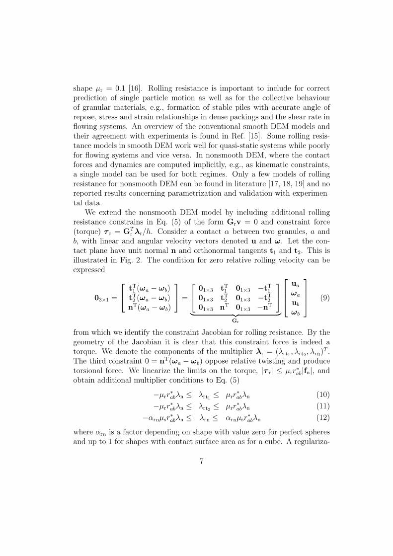
We extend the nonsmooth DEM model by including additional rollingresistance constrains in Eq. (5) of the form Grv = 0 and constraint force(torque) τ r = GT

r λr/h. Consider a contact α between two granules, a andb, with linear and angular velocity vectors denoted u and ω. Let the con-tact plane have unit normal n and orthonormal tangents t1 and t2. This isillustrated in Fig. 2. The condition for zero relative rolling velocity can beexpressed

03×1 =

tT1 (ωa − ωb)tT2 (ωa − ωb)nT(ωa − ωb)

=

01×3 tT1 01×3 −tT101×3 tT2 01×3 −tT201×3 nT 01×3 −nT

︸ ︷︷ ︸

Gr

ua

ωa

ub

ωb

(9)

from which we identify the constraint Jacobian for rolling resistance. By thegeometry of the Jacobian it is clear that this constraint force is indeed atorque. We denote the components of the multiplier λr = (λrt1 , λrt2 , λrn)

T .The third constraint 0 = nT(ωa − ωb) oppose relative twisting and producetorsional force. We linearize the limits on the torque, |τ r| ≤ µrr

∗ab|fn|, and

obtain additional multiplier conditions to Eq. (5)

−µrr∗abλn ≤ λrt1 ≤ µrr

∗abλn (10)

−µrr∗abλn ≤ λrt2 ≤ µrr

∗abλn (11)

−αrnµsr∗abλn ≤ λrn ≤ αrnµsr

∗abλn (12)

where αrn is a factor depending on shape with value zero for perfect spheresand up to 1 for shapes with contact surface area as for a cube. A regulariza-

7

tion term Σr is added to the new diagonal block in H, see Appendix A, andthe corresponding components in b are set to zero.

3. Identification of iron ore green pellet parameters

The identified parameters for onsize iron ore green pellets are summarizedin Table 1.

3.1. Mass and geometry

Iron ore green pellet have mass density of about 3700 kg/m3. The shapeis approximately spherical with diameter ranging between 9 and 16 mm andshape factor 1 in the range 0.7− 0.95.

3.2. Elasticity

The elasticity and strength of iron ore green pellets was investigatedby Forsmo et al [20]. Assuming a relation between pressure force fn andcompression δ of the form of Hertz contact law, fn = knδ

3/2, we iden-tify kn = (0.35 ± 0.05) × 106, which translates to Young’s modulus E =3kn(1 − ν2)/

√2d = 6.2 ± 0.7 MPa , see Fig. 3. We assume Poisson ratio

ν = 0.25.

3.3. Restitution

The coefficient of restitution is identified from drop tests where ore greenpellets impact on a surface coated with a 10 mm thick layer of ore materialpacked to similar density as of ore green pellets, see Fig. 4. The green pelletwas released from height 0.45 m and bounces to a height of 12 ± 4 mm,which implies an impact velocity v− = 2.97 m/s and a post impact velocityv+ = 0.49 ± 0.08 m/s. The coefficient of restitution e = −v+/v− is thusfound to be e = 0.18± 0.04.

3.4. Surface friction

The friction coefficient, µs, between two ore surfaces is identified by mea-suring the required force f for pulling a block of packed ore over a surfaceof packed ore, see Fig. 5. From the Coulomb law, f = µsmgacc, we findµs = 0.91± 0.04

1The shape factor of a cross-section of area A and perimeter length L is 4πA/L2. Asphere has shape factor 1 and a square has roughly 0.78.

8

3.5. Rolling resistance

The rolling resistance coefficient is determined from observing the angleφr at which the ore green pellet starts to roll down an inclined plane. Weobserve φr = 17.8 ± 0.1. With τ r = (d/2) sin(φr)fn we thus identify therolling resistance coefficient to µr = 0.32± 0.02.

4. Verification of simulated pellets

Material parameters in Table 1 are translated to simulation parametersof NDEM according to Sec. 2.2 and verified in elementary tests describedbelow. The results are summarized in Table 2. Simulation parameters areset to ∆t = 0.01 s, Nit = 150 if nothing else is stated.

4.1. Elasticity

The elasticity model is verified in simulation by compressing a pelletbetween a moving piston and a static plane. The piston moves in 0.02 mm/stowards to the plane. The measured constraint force GT

nλn/∆t coincidewith the Hertz model with an effective elasticity coefficient keff = fn/δ

3/2

deviating from kn with maximally 2% at δ/d = 0.1 for time step ∆t = 5 ms.The deviation decrease for smaller overlap and with decreasing time step.In the case of a single particle compressed towards to the static ground byexternal force, the result match to machine precision.

4.2. Restitution

The impact model is verified by measuring the re-bounce height hb fromdropping particles from height hd and computing the effective coefficientof restitution eeff =

√

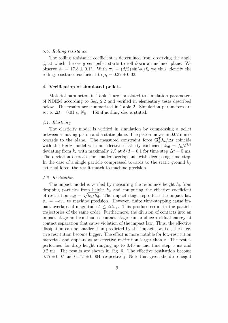
hb/hd. The impact stage reproduce the impact lawv+ = −ev− to machine precision. However, finite time-stepping cause im-pact overlaps of magnitude δ ≤ ∆tv+. This produce errors in the particletrajectories of the same order. Furthermore, the division of contacts into animpact stage and continuous contact stage can produce residual energy atcontact separation that cause violation of the impact law. Thus, the effectivedissipation can be smaller than predicted by the impact law, i.e., the effec-tive restitution become bigger. The effect is more notable for low-restitutionmaterials and appears as an effective restitution larger than e. The test isperformed for drop height ranging up to 0.45 m and time step 5 ms and0.2 ms. The results are shown in Fig. 6. The effective restitution become0.17± 0.07 and 0.175± 0.004, respectively. Note that given the drop-height

9

0.45 m and an error tolerance of ǫ = 2%, the time-step rule ∆t . ǫd/vn imply∆t = 0.4 ms. The time-step 5 ms, on the other hand, correspond to an errortolerance of ǫ = 100%. The verification results are thus in good agreementwith these error estimates but it is clear that using too large time-step maycause significant errors in energy dissipation at impacts.

4.3. Surface friction

The surface friction model is verified by simulating a pellet being pressedtowards a static plane and pulled horizontally until it starts to slide. The ef-fective friction coefficient is computed as the ratio of the horizontally appliedforce at slide onset over applied normal pressure, µs,eff = ft/fn. The resultagree with µs to machine precision.

4.4. Rolling resistance

As verification of rolling resistance we measure the maximum angle φr

where a simulated ore green pellet doesn’t start rolling on an inclined planeand compute the effective rolling resistance coefficient µr,eff = sin(φr). Theresult is φr = 17.84 and µr,eff = 0.31, to be compared to the correspondingvalues 17.8± 1 and 0.32 from experiment. The discrepancy is due to trun-cation error of the residual in the Gauss-Seidel solver but is of no practicalsignificance to the results in the paper. As a complementary verification test,we simulate the deceleration of a fast rolling pellet on a horizontal plane as-suming no-slip. The result agree with the analytical solution v = −5

7µrgacc

to machine precision.

5. Observed bulk behaviour of iron ore green pellets

We use two on-line production balling circuits at LKAB pelletizing plantin Malmberget, Sweden, for observation and validation of iron ore green pelletbulk behaviour. The circuits, referred to as rk1 and rk5, are identical butrun with different feed rate. The balling process was described in Sec. 2.1and the balling circuit is illustrated in Fig. 7. The key parameters are givenin table 3. We observe and validate three bulk properties: the angle of reposeof static piles on the conveyor of on-size pellets, the properties of the flowinside the balling drum and the spatial distribution of material on the wide-belt conveyor that results from the interaction of the flow with the outletgeometry.

10

5.1. Pile shape

The resting angle of repose, θr, is measured on the conveyor belt trans-porting on-size green pellets from the balling circuit to the induration furnace.An elongated pile is formed on the conveyor by feeding material from anotherconveyor, aligned perpendicularly to the first. The drop height is 0.3 m andfeed rate 14.4 ton/h. The pile formation is filmed with high-speed cameras,see Fig.8. The average angle of repose of the pile is found to be θr = 34± 3.

5.2. Flow in an inclined drum

The flow inside balling drum rk1 was observed during 30 minutes ofstable production of green ore pellets. A camera was placed at the end ofthe outlet to capture the flow inside the drum , see. Fig. 9. The drum wasfed with mass rate Mrk1 = 340 ton/h divided in 110 ton/h iron fines mixedwith binding agents and 230 ton/h return feed of undersized material. Thedrum rotation produce a circulating flow that is nearly stationary and in therolling or cascading regime [21]. At the bottom of the drum the materialform a plug zone where ore pellets co-move rigidly with the drum rotation.The material is lifted up to some maximal angle θ1 where particles begin toslide and form a shear zone of a gravity driven flow on top of the plug zonedown to the drum bottom at angle θ2, Fig. 9. The dynamic angle of reposeis identified by the surface inclination, i.e., θ′r = 180 − 1

2(θ1 + θ2).

From camera measurements it is found θ1 = 120± 2, θ2 = 167± 2 andθ′r = 35±5. The inclination of the drum also lead to an axial transportationflow, presumably localized to the shear zone. Cloth tracers are dropped intothe drum and tracked by camera in order to measure the surface velocityof the bulk flow, vs, and its axial and cross-sectional components, vsz andvs⊥. The measurement region is limited by the angles θ3 and θ4 and betweenthe drum center and beginning of the outlet, as indicated in Fig. 10. Themeasurement results are found in Table 4. The measurement of θ1 and θ2is based on a 100 s recording. The surface velocity is computed by time-of-flight from 10 passages of cloth tracers over the measurement region. Wecompute the axial bulk transportation velocity as vtr = M/ρAχ, where A ∈[Amin, Amax] is the bulk cross-section area and χ is the packing ratio. Theupper and lower bounds of the cross-section area are determined by assumingeither the shape of circle sector or of an annulus sector, both limited by θ1and θ2, see Fig, 10. This give Amin = 0.18 m2 and Amax = 0.27 m2. Thepacking ratio is assumed χ = 0.7.

11

The video material also reveal that the drum interior is not perfectlycylindrical but has a structure of bumps and dimples formed by fine materialadhering and loosening from drum interior surface, see Fig. 9. This drum tex-

ture presumably lead to an increased effective surface friction, higher liftingof the material and induce more flow disturbances.

5.3. Material distribution on wide-belt conveyor

The spatial distribution of material on the wide-belt conveyor depends onthe flow structure inside the drum and of the geometric shape of the outlet.The outlet is 2.3 m long and has three spiral shaped gaps. The inner andouter width of the gaps are e1 = 4.7d and e2 = 7.9d in the z′ direction. Wedescribe the resulting material height profile by h(y, t− x/vb). The goal is aconstant height profile h(y, t−x/vb) = h0 which is presumed to maximize theefficiency of the roller sieve. The flow of material at the end of the wide-beltconveyor, x = 0, is captured using video camera over a time period of 16s. The height profile is extracted by image analysis using feature matchingto localize the conveyor belt and color gradient for tracking the materialsurface. A sample is shown in Fig. 11. A 2D height profile h(y, t− x/vb) isreconstructed for comparison with simulations in Sec. 6. The time averagedprofile at x = 0 is computed as

h(y) = 1t2−t1

∫ t2

t1

h(y, t)dt (13)

The result from rk1 and rk5 are found in Fig. 18. The coefficient of variationof the height profile is

σh =

√

1wb

∫ wb

0

[h(y)− 〈h〉

〈h〉

]2

dy (14)

where 〈h〉 = 1wb

∫ wb

0h(y)dy is the average height. The observed values are

σrk1

h = 0.41 and σrk5

h = 0.33, which are acceptable although not optimal.The design objective of producing a uniform profile of pellets correspond toσh = 0.

6. Validation of the simulation model

The observations of ore green pellet flow in the balling circuit describedin Sec. 5 are used for validation of simulated bulk behaviour. The validation

12

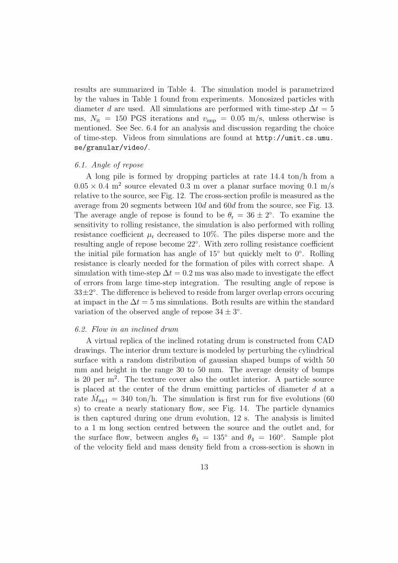
results are summarized in Table 4. The simulation model is parametrizedby the values in Table 1 found from experiments. Monosized particles withdiameter d are used. All simulations are performed with time-step ∆t = 5ms, Nit = 150 PGS iterations and vimp = 0.05 m/s, unless otherwise ismentioned. See Sec. 6.4 for an analysis and discussion regarding the choiceof time-step. Videos from simulations are found at http://umit.cs.umu.

se/granular/video/.

6.1. Angle of repose

A long pile is formed by dropping particles at rate 14.4 ton/h from a0.05 × 0.4 m2 source elevated 0.3 m over a planar surface moving 0.1 m/srelative to the source, see Fig. 12. The cross-section profile is measured as theaverage from 20 segments between 10d and 60d from the source, see Fig. 13.The average angle of repose is found to be θr = 36 ± 2. To examine thesensitivity to rolling resistance, the simulation is also performed with rollingresistance coefficient µr decreased to 10%. The piles disperse more and theresulting angle of repose become 22. With zero rolling resistance coefficientthe initial pile formation has angle of 15 but quickly melt to 0. Rollingresistance is clearly needed for the formation of piles with correct shape. Asimulation with time-step ∆t = 0.2 ms was also made to investigate the effectof errors from large time-step integration. The resulting angle of repose is33±2. The difference is believed to reside from larger overlap errors occuringat impact in the ∆t = 5 ms simulations. Both results are within the standardvariation of the observed angle of repose 34± 3.

6.2. Flow in an inclined drum

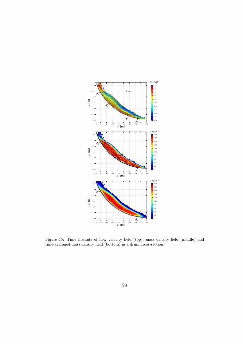
A virtual replica of the inclined rotating drum is constructed from CADdrawings. The interior drum texture is modeled by perturbing the cylindricalsurface with a random distribution of gaussian shaped bumps of width 50mm and height in the range 30 to 50 mm. The average density of bumpsis 20 per m2. The texture cover also the outlet interior. A particle sourceis placed at the center of the drum emitting particles of diameter d at arate Mrk1 = 340 ton/h. The simulation is first run for five evolutions (60s) to create a nearly stationary flow, see Fig. 14. The particle dynamicsis then captured during one drum evolution, 12 s. The analysis is limitedto a 1 m long section centred between the source and the outlet and, forthe surface flow, between angles θ3 = 135 and θ4 = 160. Sample plotof the velocity field and mass density field from a cross-section is shown in

13

Fig. 15 computed by coarse graining on a grid with mesh size of 1d. Theplug zone where material co-rotate rigidly with the drum is clearly visible.The axial transportation occur in the shear zone layer above the plug zone.The surface shape and flow is slightly irregular and nonstationary. The timeaveraged mass distribution is shown in Fig. 15. The average dynamic angleof repose is found to be θ′r = 34± 2.

The average bulk transportation velocity in the measurement region is0.22 ± 0.02 m/s. The surface between angles θ3 and θ4 is tracked over timeand the average surface velocity is found to be vs = 1.27 ± 0.09 with cross-sectional and axial components vs⊥ = 1.17± 0.09 m/s and vsz = 0.49± 0.03m/s.

To test the sensitivity to rolling resistance, the simulation is also per-formed with rolling resistance coefficient µr decreased from 0.33 to 0.03. Theeffect on the flow is significant. The dynamic angle of repose becomes 25±2

and the surface velocity vs = 0.6±0.1 with components vs⊥ = 0.43±0.1 m/sand vsz = 0.41 ± 0.03 m/s. Hence, rolling resistance is a necessary modelcomponent also for the simulated drum flow to agree with observations. Theeffect on the flow by variations of the surface friction, elasticity and particlesize was also investigated and found to be small. The time-averaged cross-sectional flow velocities and dynamic angle of repose was affected by roughly5 % by the changes µ′

s = 0.9µs, E′ = 0.5E, E ′ = 2E and d′ = 0.8d.

6.3. Material distribution on wide-belt conveyor

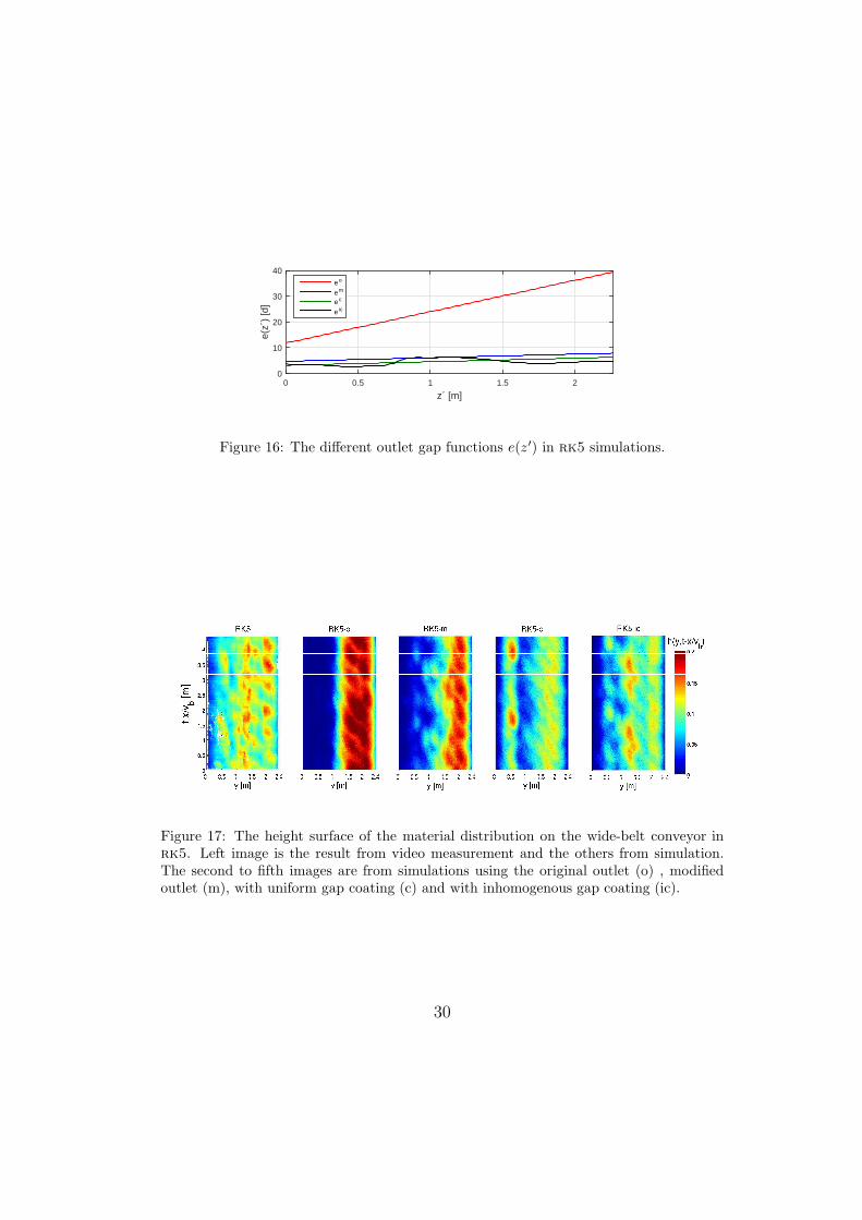
The third validation test is the distribution of ore pellets on the wide-belt conveyor below the drum outlet. This tests the predictive power ofNDEM simulation to capture the non-stationary granular flow created by theinteraction with a moving irregular geometry. Sample images from simulationis shown in Fig. 14. Simulations are performed both with the original outletdesign (rk1-o and rk5-o), in Fig. 1 and 14, with gap width eo1 : eo2 =11.8 : 39.4d, the CAD models of modified outlet that are in operation(rk1 and rk5), see Fig. 7, with em1 : em2 = 4.7 : 7.9d as well as outletgeometry models that include coating effect of fine material that make theeffective gap width smaller (rk1-c and rk5-c), ec1 : ec2 = 3.1 : 6.3d. Thegap models are illustrated in Fig. 16.

First, a stationary flow through the drum is established from a feed ofrate Mrk1. The simulations are then run for three drum evolutions, t = 36s,while recording the material distribution on the wide-belt conveyor. Thesimulations involved nearly 1 M particles for which the total computational

14

time on a 12 cpu machine become of the order 10 hours, see Eq. (8). Asample height surface from the rk5 simulation is found in Fig. 17. The time-averaged profile from rk5 and rk1 is found in Fig. 18 and the coefficients ofvariation are found in Table 4. To compare the simulated and experimentallymeasured profiles we compute also the relative coefficient of variation

σh−h =

√√√√ 4

wb

∫ wb

0

[

h(y)− h(y)

〈h〉+⟨h⟩

]2

dy (15)

where h(y) is a profile from simulation and h(y) is the profile from experi-mental observation. The simulations confirm that the original outlet model,rk5-o, was indeed a very poor design as it produce a nonuniform profilewith almost all material distributed on the right hand side of the wide-beltconveyor and σrk5−o

h = 0.83. But also the simulation with the modified CADmodel, rk5-m, distribute a substantial excess of material on the right-handside. Much more than the experimental observation from balling drums as isseen both in Fig. 17 and 18, and by the value of the relative coefficient of vari-ation σrk5−m

h−h= 0.47. The clogged outlet geometry, rk5-c, agree better with

observation, σrk5−ch−h

= 0.35, but not entirely. In the region y ∈ [1.5, 2.0] m theexperimental profile show a material depletion that has no correspondencein the simulated profile.

We hypothesize that the material depletion is due to the coating beinginhomogeneous and time-dependent. Supposedly, the coating increase grad-ually as material adheres until it reaches a critical thickness and becometoo heavy to support its own weight and drop from the outlet. We testthis by modifying the gap geometry to an inhomogeneous coating, eic(z′),as illustrated in Fig. 16. The results from the simulations with inhomoge-neous gap coating, rk5-ic, match the experimental observations fairly well,σrk5−ich−h

= 0.11.Variations in surface friction, elasticity and particle size were tested to

rule out that the deviation in material distribution is mainly due to tooimprecise material parameters. The time-averaged bed profile was affectedby roughly 5 % by the changes µ′

s = 0.9µs and E ′ = 2E. The changesE ′ = 2E and d′ = 0.8d affect the bed profile by roughly 15 %. As can beexpected, with smaller particles the bed is shifted more to the right. Theeffect is significant but not enough to explain the deviation from the observedprofile. The sensitivity of time-step size is considered in the next subsection.

15

6.4. Dependency on time-step size

The balling circuit simulations are run with time-step ∆t = 5 ms. Thischoice is based on the formula Eq. (7) and an assumed impact normal velocityvn ∼ 0.02 m/s and error tolerance ǫ = 0.01. This assumed impact velocity ischaracteristic for flow in a drum with rotation speed ωd = 0.53 rad/s, causinga characteristic shear rate σ ∼ 2ω/[1 − cos(θ/2)], where the circular sectorangle is θ = θ2 − θ1. There are impacts with higher contact velocity in thesystem but we assume the statistical occurrence of these are small and theirerror contribution to the overall bulk behaviour is insignificant. On the otherhand, as found in Sec. 4, using too large time-step may lead to significanterrors in the energy dissipation for impacts. Adapting the time-step forhigh velocity would have severe effects for the computational time. Particlesimpacting with the pellet bed on the wide-belt conveyor, for instance, havevelocity up to

√2gacchdb ∼ 3 m/s. The required time-step for maintaining

an error tolerance of ǫ = 0.01 for these contacts is 0.04 ms.The distribution of impact velocity and contact overlap from a simulation

with ∆t = 5 ms of material flowing from the drum onto the belt conveyor arepresented in histograms in Fig. 19. Analysis show that 7% of the contactsare impacts, i.e., occur with relative normal velocity higher than vimp = 0.05m/s and less than 0.01 % has velocity higher than 1 m/s. The majorityof contact overlap are below the error tolerance ǫ = 0.02 but 17 % of thecontacts have larger overlap. The overlap range up to 2d, which is consistentwith the impact velocity between particles and drum, or conveyor, rangingup to 5 m/s.

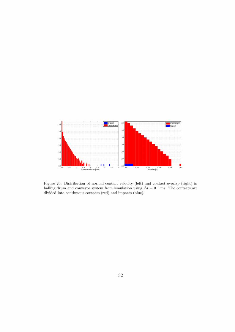
To verify the assumption that ∆t = 5 ms is indeed a valid time-stepand that the errors from high-velocity contacts do not have a significantcontribution to the bulk behaviour, a simulation was also run with time-step∆t = 0.1 ms. The drum flow characteristics are θ′r = 33±2, vtr = 0.23±0.03m/s, vs = 1.0 ± 0.1, vsz = 0.45 ± 0.03 m/s and vs⊥ = 0.9 ± 0.1 m/s for therk1. This is in good agreement with both the experimental observationand with the ∆t = 5 ms simulations in Table 4. Histograms of the contactnormal velocity and overlap from the ∆t = 0.1 ms simulation is found inFig. 20. At finer time-discretization more contact events can be resolvedin time. The impact threshold vimp = ǫd/∆t become roughly 2.5 m/s, i.e.,essentially all contacts are resolved as continuous contacts. Furthermore, inthis regime the time-step is small enough for the normal contact dissipationto be resolved with the physical viscosity from Hertz contact law, i.e., τn =max(ns∆t, εn/γn) become εn/γn = c/eH. We identified c ≈ 1 ms, from the

16

high-speed camera measurements in Fig. 4. These adjustments of vimp andτn with time-step are important. Otherwise the small time-step simulationmodel become too dissipative and produce a flow that does not agree wellwith observations.

7. Conclusions

A successful parameterization, verification and validation of a NDEMmodel for iron ore green pellets for the design and control of balling circuitshas been demonstrated. The parameterization consists in the direct identi-fication of individual ore green pellet physical parameters. The procedureinvolves no parameter calibration. The simulated bulk behaviour in the for-mation of piles and flow in a rotating inclined drum agrees with camera-basedmeasurements in the pelletizing plant. The angle of repose agrees within 5%and the flow velocity within 10 %. The pellet distribution on the wide-beltconveyor from the drum outlet show a more significant discrepancy betweensimulation and real system. The proposed explanation is that the simulatedand actual outlet geometry do not agree although they are based on the sameCAD model. Observations reveals that fine material adheres to the inside ofthe drum and outlet, creating a thick coating that alters the geometry. Inparticular, the outlet gaps become more narrow. Simulations confirm thatthe outlet flow is sensitive to this effect and that the material distributionproduced by outlet geometries where this is included agree better with obser-vation. The coating is believed to be dynamic in nature, gradually increasingin thickness until it breaks and drop, making the outlet gap narrowing vari-able and inhomogeneous. This has the consequence that even if a stationaryflow inside the drum can be achieved, the material distribution on wide-beltconveyor and roller sieve will nevertheless have variations. The conclusion isthat the outlet should be designed with materials and geometric shape whichminimize the amount of coating or at least minimize the variability and effecton the flow.

The sensitivity of the simulation model to parameters is also investigated.It is shown that the rolling resistance is a necessary component of the modelto obtain stable piles and the rolling resistance coefficient significantly affectthe shape of piles as well as the flow characteristics in the rotating drum.The drum flow is found not to be sensitive to particle size. For an accurateconveyor bed profile beneath the outlet the detailed outlet geometry and

17

rolling resistance are the critical parameters, but next to this the particlesize was also found to be important.

It is also demonstrated that using time-step as large as 5 ms do notcause any statistically significant errors to the bulk behaviour as comparedto using 0.1 ms although the larger time-step occasionally produce largeerrors in contacts between individual particles. As contrast, a conventionalDEM simulation would require a time-step of size ∆tDEM ≤ 0.17

√

m/kn[22], which evaluates to 0.02 ms for the given material parameters. Hence,NDEM simulation provide a time-efficient and reliable tool for exploring andoptimizing the design and control of iron ore pellet balling drums and ofsimilar systems. Future work should include extension to nonuniform andvariable size distribution of ore green pellets and modeling of the mixingwith ore slurry and the agglomeration process inside the drum.

Acknowledgements

This project was supported by Algoryx Simulations, LKAB, UMIT Re-search Lab and VINNOVA (dnr 2012-01235, 2014-01901).

Appendix

A. Simulation algorithm

The algoritm for simulating a system of granular material using NDEMwith PGS solver is given in Algorithm 1. The projection on line 14 limitthe multipliers to the Signorini-Coulomb law. Each contact α between bodya and b add contributions to the constraint vector and normal and frictionJacobians according to

δ(α) = nT(α)(xa + d(α)

a − xb − d(α)b )

g(α) = δeH(α)

G(α)na = eHg

eH−1(α)

[

−nT(α) −(d

(α)a × n(α))

T]

G(α)nb = eHg

eH−1(α)

[

nT(α) (d

(α)b × n(α))

T]

(16)

G(α)ta =

[

−t(α)T1 −(d

(α)a × t

(α)1 )T

−t(α)T2 −(d

(α)a × t

(α)2 )T

]

G(α)tb =

[

t(α)T1 (d

(α)b × t

(α)1 )T

t(α)T2 (d

(α)b × t

(α)2 )T

]

18

Algorithm 1 NDEM simulation with PGS solver

1: constants and parameters2: initialization: (x0,v0)3: for i = 0, 1, 2, . . . , t/∆t do ⊲ Time stepping4: contact detection5: compute g,G,Σ,Υ,D, see Eq. (18)6: impact stage PGS solve vi → (v+

i ,λ+i )

7: bn = −(4/∆t)Υngn +ΥnGnv+i

8: pre-step v = v+i +∆tM−1fext

9: for k = 0, 1, . . . , Nit − 1 or |r| ≤ rmin do ⊲ PGS iteration10: for each contact α = 0, 1, . . . , Nc − 1 do

11: for each constraint n of contact α do

12: r(α)n,k = −b

(α)n,k +G(α)

n v ⊲ residual

13: λ(α)n,k = λ

(α)n,k−1 +D−1

n,(α)r(α)n,k ⊲ multiplier

14: proj(λ(α)n,k,v) → λ

(α)n,k ⊲ project

15: ∆λ(α)n,k = λ

(α)n,k − λ

(α)n,k−1

16: v = v +M−1GTn,(α)∆λ

(α)n,k

17: end for

18: end for

19: end for

20: vi+1 = v ⊲ velocity update21: xi+1 = xi +∆tvi+1 ⊲ position update22: end for

The diagonal matrices and Schur complement matrix D are

Σn =4

∆t2εn

1 + 4 τn∆t

1Nc×Nc

Σt =γt∆t

12Nc×2Nc

Σr =γr∆t

13Nc×3Nc(17)

Υn =1

1 + 4 τn∆t

1Nc×Nc

D = GM−1GT +Σ

19

The mapping between regularization parameters and material parametersare

εn = eH/kn = 3eH(1− ν2)/E√r∗

τn = max(ns∆t, εn/γn) (18)

γ−1n = knc/e

2H

and we use γt = γr = 10−6, ns = 2.

References

[1] F. Radjai, V. Richefeu, Contact dynamics as a nonsmooth discrete ele-ment method, Mechanics of Materials 41 (6) (2009) 715–728.

[2] M. Servin, D. Wang, C. Lacoursiere, K. Bodin, Examining the smoothand nonsmooth discrete element approach to granular matter, Int. J.Numer. Meth. Engng. 97 (2014) 878–902.

[3] D. Wang, M. Servin, K.-O. Mickelsson, Outlet design optimization basedon large-scale nonsmooth DEM simulation, Powder Technology 253 (0)(2014) 438–443.

[4] S. Forsmo, Influence of green pellet properties on pelletizing of magnetiteiron ore, Ph.D. thesis, Lulea University of Technology, Lulea (2007).

[5] I. Cameron, F. Wang, C. Immanuel, F. Stepanek, Process systems mod-elling and applications in granulation: A review, Chemical EngineeringScience 60 (14) (2005) 3723–3750.

[6] R. Soda, A. Sato, J. Kano, E. Kasai, F. Saito, M. Hara, T. Kawaguchi,Analysis of granules behavior in continuous drum mixer by DEM, ISIJInternational 49 (5) (2009) 645–649.

[7] T. Poschel, T. Schwager, Computational Granular Dynamics, Modelsand Algorithms, Springer-Verlag, 2005.

[8] J. J. Moreau, Numerical aspects of the sweeping process, ComputerMethods in Applied Mechanics and Engineering 177 (1999) 329–349.

[9] M. Jean, The non-smooth contact dynamics method, Computer Meth-ods in Applied Mechanics and Engineering 177 (1999) 235–257.

20

[10] F. A. Bornemann, C. Schutte, Homogenization of Hamiltonian systemswith a strong constraining potential, Phys. D 102 (1-2) (1997) 57–77.

[11] N. V. Brilliantov, F. Spahn, J.-M. Hertzsch, T. Poschel, Model for col-lisions in granular gases, Phys. Rev. E 53 (1996) 5382–5392.

[12] C. Lacoursiere, Regularized, stabilized, variational methods for multi-bodies, in: D. F. Peter Bunus, C. Fuhrer (Eds.), The 48th ScandinavianConference on Simulation and Modeling (SIMS 2007), Linkoping Uni-versity Electronic Press, 2007, pp. 40–48.

[13] K. G. Murty, Linear Complementarity, Linear and Nonlinear Program-ming, Helderman-Verlag, Heidelberg, 1988.

[14] Algoryx Simulations. AGX Dynamics, December 2014.

[15] J. Ai, J.-F. Chen, J. M. Rotter, J. Y. Ooi, Assessment of rolling resis-tance models in discrete element simulations, Powder Technology 206 (3)(2011) 269–282.

[16] N. Estrada, E. Azema, F. Radjai, A. Taboada, Identification of rollingresistance as a shape parameter in sheared granular media, Phys. Rev.E 84 (2011) 011306.

[17] N. Estrada, A. Taboada, F. Radjaı, Shear strength and force transmis-sion in granular media with rolling resistance, Phys. Rev. E 78 (2008)021301.

[18] J. Huang, M. V. da Silva, K. Krabbenhoft, Three-dimensional granularcontact dynamics with rolling resistance, Computers and Geotechnics49 (0) (2013) 289–298.

[19] A. Tasora, M. Anitescu, A complementarity-based rolling friction modelfor rigid contacts, Meccanica 48 (7) (2013) 1643–1659.

[20] S. Forsmo, P.-O. Samskog, B. Bjorkman, A study on plasticity andcompression strength in wet iron ore green pellets related to real processvariations in raw material fineness, Powder Technology 181 (3) (2008)321–330.

21

Figure 1: Image from simulation of balling drum with green ore pellets flowing throughthe outlet gaps onto the wide-belt conveyor feeding the roller sieve.

[21] H.-T. Chou, C.-F. Lee, Cross-sectional and axial flow characteristics ofdry granular material in rotating drums, Granular Matter 11 (1) (2008)13–32.

[22] C. O. J. Bray, Selecting a suitable time step for discrete element simula-tions that use the central difference time integration scheme, EngineeringComputations 21 (2/3/4) (2004) 278–303.

22

b

a

τr

t

tn

1

2

fn

ft

Figure 2: Illustration of two contacting granular geometries a and b. Rolling resistanceconstraint produce a torque, τ r, limited in magnitude relative to the normal contact forcefn in a similar way as the Coulomb friction force ft.

Figure 3: Measurement of elasticity and strength of iron ore green pellets from Forsmo etal in Ref. [20] Fig. 1 and 13c.

23

Figure 4: Measurement of coefficient of restitution by impacting ore green pellet capturedat 100 Hz.

Figure 5: Measurement of surface friction (left) and rolling resistance (right).

24

0 0.05 0.1 0.15 0.2 0.25 0.3 0.35 0.4 0.45 0.50

0.05

0.1

0.15

0.2

0.25

0.3

0.35

0.4

Drop height [m]

Effe

ctiv

e re

stitu

tion

h=5ms

h=0.2ms

Ref: e=0.18

Figure 6: Verification of the impact model by measuring the effective restitution.

wide belt

conveyor

y

x

undersize

onsizeroller sieve

drum

outlet

z

fines

v

wb

b

e1

e2

ωdβd

hdb

oversize

z'

Figure 7: Illustration of the balling circuit.

25

Figure 8: Photos from angle of repose measurement.

Figure 9: Sample images of drum interior (left and middle) and distribution on wide-beltconveyor (right). The bulk flow of ore pellets circulate in the lower left section of the drum.The fine material adhere to the drum walls and form an irregular surface coating. Themiddle image show a close-up of the irregular drum surface and coating of fine materialaround the outlet gaps.

Figure 10: Pellet flow in rotating inclined drum.

26

Figure 11: Sample images from extraction of height profile on wide-belt conveyor in rk5.

Figure 12: Images from simulation of pile formation.

−0.1 −0.05 0 0.05 0.1

0.02

0.03

0.04

0.05

0.06

0.07

0.08

0.09

0.1

x [m]

z [m

]

Slope profile µ

r=0

Slope profile µr=0.03

Slope profile µr=0.32

Figure 13: The average pile profile and its linear interpolation for different values of rollingresistance. For µr = 0 the pile quickly disperse to zero angle of repose.

27

Figure 14: Image from simulation showing material distribution inside drum (top) and onthe wide-belt conveyor (bottom). The original outlet deisgn is used. Particles are colorcoded by velocity and height, respectively.

28

1 m/s

−1.8 −1.6 −1.4 −1.2 −1.0 −0.8 −0.6 −0.4 −0.2 0.0

x′ [m]

−2.2

−2.0

−1.8

−1.6

−1.4

−1.2

−1.0

y′ [m

]

θ1

θ2

θ3

θ4 −0.8

−0.7

−0.6

−0.5

−0.4

−0.3

−0.2

−0.1

0.0

0.1

0.2

Vz′ [m/s]

−1.8 −1.6 −1.4 −1.2 −1.0 −0.8 −0.6 −0.4 −0.2 0.0

x′ [m]

−2.2

−2.0

−1.8

−1.6

−1.4

−1.2

−1.0

y′ [m

]

θ1

θ20

200

400

600

800

1000

1200

1400

1600

1800

2000

ρ [kg/m3 ]

−1.8 −1.6 −1.4 −1.2 −1.0 −0.8 −0.6 −0.4 −0.2 0.0

x′ [m]

−2.2

−2.0

−1.8

−1.6

−1.4

−1.2

−1.0

y′ [m

]

θ1

θ20

200

400

600

800

1000

1200

1400

1600

1800

2000

ρ [kg/m3 ]

Figure 15: Time instants of flow velocity field (top), mass density field (middle) andtime-averaged mass density field (bottom) in a drum cross-section.

29

z´ [m]0 0.5 1 1.5 2

e(z´

) [d

]

0

10

20

30

40eo

em

ec

e ic

Figure 16: The different outlet gap functions e(z′) in rk5 simulations.

Figure 17: The height surface of the material distribution on the wide-belt conveyor inrk5. Left image is the result from video measurement and the others from simulation.The second to fifth images are from simulations using the original outlet (o) , modifiedoutlet (m), with uniform gap coating (c) and with inhomogenous gap coating (ic).

30

0.0 0.5 1.0 1.5 2.0y [m]

0.0

0.1

0.2

h(y) [m

]

RK1-o

RK1-m

RK1-c

RK1-ic

RK1

0.0 0.5 1.0 1.5 2.0y [m]

0.0

0.1

0.2

h(y) [m

]

RK5-o

RK5-m

RK5-c

RK5-ic

RK5

Figure 18: The time averaged height profile on the wide-belt conveyor from rk1 and rk5.The dashed line is the result from video measurement. The solid lines are from simulationsusing the original outlet (o) , modified outlet (m), with uniform gap coating (c) and withinhomogenous gap coating (ic).

0 1 2 3 4 510

0

101

102

103

104

105

106

107

Contact velocity [m/s]

ImpactContinuous

0 0.5 1 1.510

0

101

102

103

104

105

106

107

Overlap [d]

ContinuousImpact

Figure 19: Distribution of normal contact velocity (left) and contact overlap (right) inballing drum and conveyor system from simulation using ∆t = 5 ms. The contacts aredivided into continuous contacts (red) and impacts (blue).

31

0 0.5 1 1.5 2 2.5 3 3.5 410

0

101

102

103

104

105

106

Contact velocity [m/s]

ImpactContinuous

0 0.02 0.04 0.06 0.08 0.110

0

101

102

103

104

105

106

Overlap [d]

ContinuousImpact

Figure 20: Distribution of normal contact velocity (left) and contact overlap (right) inballing drum and conveyor system from simulation using ∆t = 0.1 ms. The contacts aredivided into continuous contacts (red) and impacts (blue).

32

Table 1: Identified iron ore green pellet parameters.

ρ 3700 kg/m3 mass densityd 12.7± 3 mm diameterE 6.2± 0.7 MPa Young’s moduluse 0.18± 0.04 coefficient of restitutionµs 0.91± 0.04 surface friction coefficientµr 0.32± 0.02 rolling resistance coefficient

Table 2: Summary of results from verification tests.Test Quantity Result Comment

Elasticity ‖keff − k‖/k 0− 2% error 2% at ρ/d & 0.1 and ∆t & 5 ms

Restitution ‖eeff − e‖/e 1% ∆t . min(ǫd/vn,√

2ǫd/g) and ǫ =0.01

Friction ‖µeff − µ‖/µ 0% fulfilled to machine precisionRolling resistance ‖µr,eff − µr‖/µr 0− 1% 1% error at rolling onset.

Table 3: Specification of balling circuit parameters.Notation Value Parameter

ωd 0.53 rad/s drum rotation speedβd 7 drum inclinationD 3.7 m drum inner diameterL 8.1 m drum lengthe1 : e2 4.7 : 7.9 d inner : outer gap widthwb 2.4 m width of wide-belt conveyorvb 0.19 m/s speed of wide-belt conveyorhdb 0.45 m distance drum to conveyor

Mrk1 340 ton/h mass flow rate in rk1

Mrk5 275 ton/h mass flow rate in rk5

33

Table 4: Validation of simulated bulk behaviour by comparing with observations in ballingcircuits.

Test Quantity Observation Simulation

Pile shape θr 34± 3 36± 2

Drum flow θ′r 35± 5 34± 2

vtr 0.20± 0.03 m/s 0.22± 0.02 m/svs 1.31± 0.06 m/s 1.27± 0.09 m/svsz 0.58± 0.05 m/s 0.49± 0.03 m/svs⊥ 1.18± 0.07 m/s 1.17± 0.09 m/s

Bed profile rk1 σh 0.41rk1-o 0.83rk1-m 0.66rk1-c 0.46rk1-ic 0.44

σh−h 0rk1-o 1.01rk1-m 0.81rk1-c 0.54rk1-ic 0.27

Bed profile rk5 σh 0.33rk5-o 0.83rk5-m 0.68rk5-c 0.42rk5-ic 0.42

σh−h 0rk5-o 0.71rk5-m 0.47rk5-c 0.35rk5-ic 0.11

34