Convergence of Newton's Method for Singular Smooth andNonsmooth Equations Using Adaptive Outer Inverses 1Xiaojun ChenSchool of Mathematics, University of New South WalesSydney 2052, AustraliaZuhair NashedDepartment of Mathematical Sciences, University of DelawareNewark, DE 19716, USALiqun QiSchool of Mathematics, University of New South WalesSydney 2052, Australia(January 1993, Revised June 1995)ABSTRACT.We present a local convergence analysis of generalized Newton meth-ods for singular smooth and nonsmooth operator equations using adaptive constructsof outer inverses. We prove that for a solution x� of F (x) = 0, there exists a ballS = S(x�; r), r > 0 such that for any starting point x0 2 S the method converges toa solution �x� 2 S of �F (x) = 0, where � is a bounded linear operator that dependson the Fr�echet derivative of F at x0 or on a generalized Jacobian of F at x0. Point�x� may be di�erent from x� when x� is not an isolated solution. Moreover, we provethat the convergence is quadratic if the operator is smooth, and superlinear if theoperator is locally Lipschitz. These results are sharp in the sense that they reducein the case of an invertible derivative or generalized derivative to earlier theoremswith no additional assumptions. The results are illustrated by a system of smoothequations and a system of nonsmooth equations, each of which is equivalent to anonlinear complementarity problem.Key words: Newton's method, convergence theory, nonsmooth analysis, outer in-verses, nonlinear complementarity problems.AMS(MOS) subject classi�cation. 65J15, 65H10, 65K10, 49M15.Abbreviated title: Newton's method for singular equations1This work is supported by the Australian Research Council and by the National Science Foun-dation Grant DMS-901526. 1

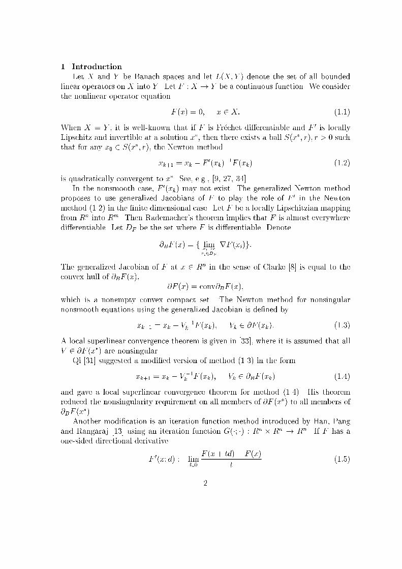
1. IntroductionLet X and Y be Banach spaces and let L(X; Y ) denote the set of all boundedlinear operators on X into Y . Let F : X ! Y be a continuous function. We considerthe nonlinear operator equationF (x) = 0; x 2 X: (1:1)When X = Y , it is well-known that if F is Fr�echet di�erentiable and F 0 is locallyLipschitz and invertible at a solution x�, then there exists a ball S(x�; r); r > 0 suchthat for any x0 2 S(x�; r), the Newton methodxk+1 = xk � F 0(xk)�1F (xk) (1:2)is quadratically convergent to x�. See, e.g., [9, 27, 34].In the nonsmooth case, F 0(xk) may not exist. The generalized Newton methodproposes to use generalized Jacobians of F to play the role of F 0 in the Newtonmethod (1.2) in the �nite dimensional case. Let F be a locally Lipschitzian mappingfrom Rn into Rm. Then Rademacher's theorem implies that F is almost everywheredi�erentiable. Let DF be the set where F is di�erentiable. Denote@BF (x) = f limxi!xxi2DF rF (xi)g:The generalized Jacobian of F at x 2 Rn in the sense of Clarke [8] is equal to theconvex hull of @BF (x), @F (x) = conv@BF (x);which is a nonempty convex compact set. The Newton method for nonsingularnonsmooth equations using the generalized Jacobian is de�ned byxk+1 = xk � V �1k F (xk); Vk 2 @F (xk): (1:3)A local superlinear convergence theorem is given in [33], where it is assumed that allV 2 @F (x�) are nonsingular.Qi [31] suggested a modi�ed version of method (1.3) in the formxk+1 = xk � V �1k F (xk); Vk 2 @BF (xk) (1:4)and gave a local superlinear convergence theorem for method (1.4). His theoremreduced the nonsingularity requirement on all members of @F (x�) to all members of@BF (x�).Another modi�cation is an iteration function method introduced by Han, Pangand Rangaraj [13] using an iteration function G(�; �) : Rn � Rn ! Rn. If F has aone-sided directional derivativeF 0(x; d) := limt#0 F (x+ td)� F (x)t (1:5)2

and G(x; d) = F 0(x; d), a variant of the iteration function method can be de�ned by( solve F (xk) + F 0(xk; d) = 0;set xk+1 = xk + d: (1:6)See also Pang [28] and Qi [31].Methods (1.2), (1.3), (1.4) and (1.6) are very useful, but they are not applicableto the singular case. At each step in (1.2), (1.3) and (1.4), the inverse of a Jacobianor a generalized Jacobian is required; in (1.6) a nonlinear equation is solved at eachstep (in the singular case, it may have no solutions). Often the inverse cannotbe guaranteed to exist; singularity occurs in many applications. For example, weconsider the nonlinear complementarity problem(NCP): For a given f : Rn ! Rn,�nd x 2 Rn such that x � 0; f(x) � 0 and xTf(x) = 0:Mangasarian [19] formulated the NCP in the case when f is Fr�echet di�erentiableas an equivalent system of smooth equations:F̂i(x) = (fi(x)� xi)2 � fi(x)jfi(x)j � xijxij = 0; i = 1; 2; :::; n; (1:7)where f = (f1; :::; fn)T : Letsgn(�) = ( 1; � � 0;�1; � < 0;and let �ij denote the Kronecker function. It is easy to show that the Jacobian ofF̂ := (F̂1; :::; F̂n)T at x is given by:@F̂i(x)@xj = 2fi(x)@fi(x)@xj (1� sgn(fi(x))) + 2xi�ij(1� sgn(xi))� 2fi(x)�ij � 2xi@fi(x)@xji; j = 1; 2; :::; n:The Jacobian rF̂ (x) is singular when there is some degeneracy, i.e. xi = fi(x) = 0for some i.The NCP can also be formulated as a system of nonsmooth equations [28] :~F (x) = min(f(x); x) = 0; (1:8)where the \min" operator denotes the componentwise minimum of two vectors. It ishard to guarantee that all members of @BF (x) are nonsingular when there is somenonsmoothness, i.e. xi = fi(x) and ei 6= rfi(x) for some i, where ei is the i-th rowof the identity matrix I 2 Rn�n. 3

In [5], Chen and Qi studied a parameterized Newton method:xk+1 = xk � (Vk + �kI)�1F (xk); Vx 2 @BF (xk);where �k is a parameter to ensure the existence of the inverse of Vk + �kI: The localsuperlinear convergence theorem in [5] requires all V� 2 @BF (x�) to be nonsingular.In Newton-like methods for solving smooth and nonsmooth equations, e.g. quasi-Newton methods and splitting methods, the Jacobian is often required to be nonsin-gular at a solution x� to which the method is supposed to converge [4, 5, 6, 9, 15,16, 27, 28, 32, 40]. Hence it is interesting to know what happens with the Newtonmethods when F 0(x�) or some V� 2 @BF (x�) are singular at x�. In this case thesolution set is locally a manifold of positive dimension, hence x� is not an isolatedsolution.Let A 2 L(X; Y ). We denote the range and nullspace of A by R(A) and N(A),respectively. A linear operator A] : Y ! X is said to be an outer inverse of A ifA]AA] = A].In this paper, forX = Rn and Y = Rm, we consider a generalized Newton methodxk+1 = xk � V ]kF (xk) (1:9)where Vk 2 @BF (xk) and V ]k denotes an outer inverse of Vk.Newton's method for singular smooth equations using outer inversesxk+1 = xk � F 0(xk)]F (xk) (1:10)has been considered by Ben-Israel [2], Deu hard and Heindl [10] and Nashed [25]and more recently by Nashed and Chen [26]. Paper [26] presented a Kantorovich-type theorem (semilocal convergence) for Newton-like methods for singular smoothequations using outer inverses : if some conditions hold at the starting point x0,method (1.10) converges to a solution of F 0(x0)]F (x) = 0.This paper establishes new results on Newton's method for smooth and nons-mooth equations. In particular we consider the behavior of methods (1.9) and (1.10)when the singularity occurs at a solution x� which is close to the starting point.In Section 2 we state the de�nitions and properties of generalized gradients, semi-smooth functions and outer inverses. These results are used to analyze convergenceof methods (1.9) and (1.10).In Section 3 by using a Kantorovich-type theorem, we give a locally quadraticconvergence theorem for Newton's method (1.10) in the following sense: for a solutionx� of (1.1), there is a ball S(x�; r) with r > 0 such that for any x0 2 S(x�; r); Newton'smethod (1.10) with F 0(xk)] = (I + F 0(x0)](F 0(xk) � F 0(x0)))�1F 0(x0)] convergesquadratically to a solution �x� of F 0(x0)]F (x) = 0. Here, �x� may be di�erent from x�,because of singularity, there is no guarantee for uniqueness of the solutions. This isa major di�erence between singular and nonsingular equations.4

In Section 4 by using a Mysovskii-type theorem we prove the superlinear conver-gence of method (1.9) for nonsmooth equations. Di�culties in the analysis of method(1.9) for singular nonsmooth equations that have not been previously resolved in theliterature arise from the fact that there are some singular elements Vx 2 @BF (x),so rank(Vx) are di�erent and V ]xVx 6= I. Previous results for nonsingular equationsrequire that all Vx 2 @BF (x) have full rank and VxV �1x = V �1x Vx = I. We developnew techniques for considering singular nonsmooth equations. It is noteworthy thatthe solution to which our method converges (in both smooth and nonsmooth cases)need not be the original solution, and our method applies even when the solution setis locally a manifold of positive dimension.In Section 5 we illustrate the singularity issue by numerical examples. We givenumerical results for computing three examples of the NCP by methods (1.9) and(1.10) via a system of smooth equations (1.7) and a system of nonsmooth equations(1.8), respectively.2. De�nitions and lemmas on outer inverses and semismooth functionsOuter inverses of linear operators play a pivotal role in the formulation and con-vergence analysis of the iterative methods studied in this paper. Their role is derivedfrom projectional properties of outer inverses and more importantly from perturba-tion and stability analysis of outer inverses. The strategy is based on Banach-typelemmas and perturbation bounds for outer inverses which show that the set of outerinverses (to a given bounded linear operator) admits selections that behave likebounded linear inverses, in contrast to inner inverses or generalized inverses whichdo not depend continuously on perturbations of the operators. This strategy was�rst used in [26] to generate adaptive constructs of outer inverses that would leadto sharp convergence results. Lemmas 2.1-2.4 below summarize important pertur-bation bounds and projectional properties of outer inverses which are used in theconvergence analysis. For detailed proofs and related properties and references, see[26]. For de�nition and properties of generalized inverses in Banach spaces, see [24]or [25].Lemma 2.1(Banach-type lemma for outer inverses). Let A 2 L(X; Y ) and let A] 2L(Y;X) be an outer inverse of A. Let B 2 L(X; Y ) be such that jjA](B � A)jj < 1.Then B] := (I+A](B�A))�1A] is a bounded outer inverse of B withN(B]) = N(A])and R(B]) = R(A]). Moreover,jjB] � A]jj � jjA](B � A)jjjjA]jj1� jjA](B � A)jjand jjB]Ajj � 11� jjA](B � A)jj :5

Lemma 2.2. Let A 2 L(X; Y ): If A] is a bounded outer inverse of A, then thefollowing topological direct sum decompositions hold:X = R(A])�N(A]A)Y = N(A])� R(AA]):Lemma 2.3. Let A;B 2 L(X; Y ) and let A] and B] 2 L(Y;X) be outer inverses ofA and B, respectively. Then B](I � AA]) = 0 if and only if N(A]) � N(B]):Lemma 2.4. Let A 2 L(X; Y ) and let Ay be a bounded generalized inverse ofA. Let B 2 L(X; Y ) satisfy the condition jjAy(B � A)jj < 1, and de�ne B] :=(I + Ay(B � A))�1Ay. Then B] is a generalized inverse of B if and only ifdimN(B) = dimN(A)and codimR(B) = codimR(A):Note that if A and B are Fredholm operators with the same index, then the twodimensionality conditions are equivalent. Thus Lemma 2.4 and Theorem 3.4 beloware not restricted to �nite dimensional spaces. A simple example of a Fredholmoperator is an operator of the form I +K, where K is a compact operator.For nonsmooth problems, we consider functions which are semismooth. We nowrecall two de�nitions and an important property related to this class of functions.De�nition 2.5. A function F : Rn ! Rm is said to be B-di�erentiable at a point xif F has a one-sided directional derivative F 0(x; h) at x (see (1.5)) andlimh!0 F (x+ h)� F (x)� F 0(x; h)k h k = 0: (2:1)We may write (2.1) as F (x+ h) = F (x) + F 0(x; h) + o(k h k):De�nition 2.6. A function F : Rn ! Rm is semismooth at x if F is locally Lipschitzat x and limV 2@F (x+th0)h0!h;t#0 fV h0gexists for every h 2 Rn.Lemma 2.7 [31]. If F : Rn ! Rm is semismooth at x, then F is directionallydi�erentiable at x and for any V 2 @F (x + h);V h� F 0(x; h) = o(jjhjj):Shapiro [36] showed that a locally Lipschitzian function F is B-di�erentiable at xif and only if it is directionally di�erentiable. Hence F is B-di�erentiable at x if F is6

semismooth at x. For a comprehensive analysis of the role of semismooth functionssee [21, 31, 33].3. Local convergence for smooth equationsS(x; r) denotes the open ball in X with center x and radius r; and �S(x; r) is itsclosure. For a �xed A 2 L(X; Y ), we denote the set of nonzero outer inverses of Aby (A) := fB 2 L(Y;X) : BAB = B;B 6= 0g:In this section we give two local convergence theorems for method (1.10) by usingthe following Kantorovich-type theorem (semilocal convergence).Theorem 3.1. Let F : D � X ! Y be Fr�echet di�erentiable. Assume that thereexist an x0 2 D, F 0(x0)] 2 (F 0(x0)) and constants �;K > 0 such that for allx; y 2 D the following conditions hold:jjF 0(x0)]F (x0)jj � � (3:1)jjF 0(x0)](F 0(x)� F 0(y))jj � Kjjx� yjj (3:2)h := K� � 12 ; S(x0; t�) � D; (3:3)where t� = (1�p1� 2h)=K: Then the sequence fxkg de�ned by method (1.10) withF 0(xk)] = (I + F 0(x0)](F 0(xk) � F 0(x0)))�1F 0(x0)] lies in S(x0; t�) and converges toa solution x� of F 0(x0)]F (x) = 0.(See Theorem 3.1 and Corollary 3.1 in [26].)Theorem 3.2. Let F : D � X ! Y be Fr�echet di�erentiable and assume thatF 0(x) satis�es a Lipschitz conditionjjF 0(x)� F 0(y)jj � Ljjx� yjj; x 2 D: (3:4)Assume that there exists an x� 2 D such that F (x�) = 0: Let p > 0 be a positivenumber such that S(x�; 1p) � D. Suppose that the following condition holds:(a) there is a F 0(x�)] 2 (F 0(x�)) such that jjF 0(x�)]jj � p and for any x 2S(x�; 13Lp) the set (F 0(x)) contains an element of minimal norm.Then there exists a ball S(x�; r) � D with 0 < r < 13Lp such that for anyx0 2 S(x�; r), the sequence fxkg de�ned by method (1.10) withF 0(x0)] 2 argminfjjBjj : B 2 (F 0(x0))g (3:5)and with F 0(xk)] = (I + F 0(x0)](F 0(xk)� F 0(x0)))�1F 0(x0)] converges quadraticallyto �x� 2 S(x0; 1Lp) \ fR(F 0(x0)]) + x0g, which is a solution of F 0(x0)]F (x) = 0: HereR(F 0(x0)]) + x0 := fx+ x0 : x 2 R(F 0(x0)])g:7

Proof. Let �r = 13Lp and � = 427Lp2 :We �rst prove that there exists a ball S(x�; r) � D; 0 < r � �r such that for anyx0 2 S(x�; r); all conditions of Theorem 3.1 hold.Since F is continuous at x�, there exists a ball S(x�; r) � D; 0 < r � �r, such thatfor any x 2 S(x�; r), jjF (x)jj < �:From (3.4), there is a F 0(x�)] 2 (F 0(x�)) such thatjjF 0(x�)](F 0(x)� F 0(x�))jj � pLr < 1:By Lemma 2.1, we have thatF 0(x)] = (I + F 0(x�)](F 0(x)� F 0(x�)))�1F 0(x�)]is an outer inverse of F 0(x) andjjF 0(x)]jj � jjF 0(x�)]jj1� pLr � p1� pLr =: �:Hence for any x0 2 S(x�; r), the outer inverseF 0(x0)] 2 argminfjjBjj : B 2 (F 0(x0))gsatis�es jjF 0(x0)]jj � �. Let K = 32�L: Then for x; y 2 D,jjF 0(x0)](F 0(x)� F 0(y))jj � �jjF 0(x)� F 0(y)jj � Kjjx� yjj;and h = KjjF 0(x0)]F (x0)jj � 32L�2� � 29(1� pLr)2 � 12 :Furthermore, for any x 2 S(x0; t�) with t� = (1�p1� 2h)=K, we havejjx� � xjj � jjx0 � x�jj+ jjx0 � xjj � 13Lp + 23L� � 13Lp + 2(1� Lpr)3Lp � 1Lp:This implies S(x0; t�) � S(x�; 1Lp) � D. Hence all conditions of Theorem 3.1 holdat x0. Thus the sequence fxkg lies in S(x0; t�) and converges to a solution �x� ofF 0(x0)]F (x) = 0:Now we prove that the convergence rate is quadratic.Since F 0(xk)] = (I+F 0(x0)](F 0(xk)�F 0(x0)))�1F 0(x0)]; by Lemma 2.1, R(F 0(x0)])= R(F 0(xk)]). By xk+1 � xk = F 0(xk)]F (xk) 2 R(F 0(xk)]);8

we have xk+1 2 R(F 0(xk)]) + xk = R(F 0(xk�1)]) + xk = R(F 0(x0)]) + x0and �x� 2 R(F 0(xk)]) + xk+1 for any k � 0. This implies that�x� 2 R(F 0(x0)]) + x0 = R(F 0(xk)]) + x0and F 0(xk)]F 0(xk)(�x� � xk+1)= F 0(xk)]F 0(xk)(�x� � x0)� F 0(xk)]F 0(xk)(xk+1 � x0) = �x� � xk+1:From Lemma 2.3, we have F 0(xk)] = F 0(xk)]F 0(x0)F 0(x0)]: Using F 0(x0)]F (�x�) = 0and N(F 0(x0)]) = N(F 0(xk)]); we obtain F 0(xk)]F (�x�) = 0 andjj�x� � xk+1jj = jjF 0(xk)]F 0(xk)(�x� � xk+1)jj= jjF 0(xk)]F 0(xk)(�x� � xk + F 0(xk)](F (xk)� F (�x�)))jj= jjF 0(xk)](F 0(xk)(�x� � xk)� Z 10 F 0(xk + t(xk � �x�))dt(�x� � xk))jj= jjF 0(xk)]F 0(x0)jjjjF 0(x0)](F 0(xk)� Z 10 F 0(xk + t(xk � �x�))dt)(�x� � xk)jj� 11�Kt� � K2 jj�x� � xkjj2:Hence xk ! �x� quadratically. 2Lemma 3.3. Let A 2 L(X; Y ); A 6= 0, where X and Y are �nite dimensional normedspaces. Then the in�mum of jjBjj over (A) is attained.Proof. Let A be a �xed nonzero linear operator from X into Y . For any nonzeroouter inverse B of A, we have jjBjj = jjBABjj � jjBjj2jjAjj; hence jjBjj � 1jjAjj: Let� :=inf fjjBjj : B 2 (A)g. There exists fBkg � (A) such that lim kBkk = �; andsince fBkg is bounded, it has a limit point B. Then BkABk = Bk and jjBkjj � 1jjAjj.Hence BAB = B and jjBjj = �. Thus (A) contains an element of minimal operatornorm. 2Theorem 3.4. Let F satisfy the assumptions of Theorem 3.2 except that condition(a) is replaced by the following condition:(b) the generalized inverse F 0(x�)y exists, kF 0(x�)yk � p and for any x 2 S(x�; 13Lp);dimN(F 0(x)) = dimN(F 0(x�))9

and codimR(F 0(x)) = codimR(F 0(x�)):Then the conclusion of Theorem 3.2 holds withF 0(x0)] 2 fB : B 2 (F 0(x0)); jjBjj � jjF 0(x0)yjjg: (3:6)Proof. Condition (a) of Theorem 3.2 ensures that for any x 2 S(x�; r); 0 < r �1=3Lp, the outer inverse F 0(x)] 2 argminfkBk : B 2 (F 0(x))g satis�es kF 0(x)]k �p=(1 � Lpr): Now we show that under condition (b), for any x 2 S(x�; r); 0 < r �1=3Lp; the outer inverse F 0(x)] 2 fB : B 2 (F 0(x)); jjBjj � jjF 0(x)yjjg satis�eskF 0(x)]k � p=(1� Lpr):From (3.4),jjF 0(x�)y(F 0(x)� F 0(x�))jj � pjjF 0(x)� F 0(x�)jj � pLjjx� x�jj � pLr < 1:By Lemma 2.4, F 0(x)y = (I + F 0(x�)y(F 0(x)� F 0(x�)))�1F 0(x�)yis the generalized inverse of F 0(x). By Lemma 2.1,jjF 0(x)yjj � jjF 0(x�)yjj1� pLr � p1� pLr =: �:Hence for any x0 2 S(x�; r), the outer inverseF 0(x0)] 2 fB : B 2 (F 0(x0)); jjBjj � jjF 0(x0)yjjgsatis�es jjF 0(x0)]jj � �. By the same argument in the proof of Theorem 3.2, we canshow the conclusion of Theorem 3.2 holds withF 0(x0)] 2 fB : B 2 (F 0(x0)); kBk � kF (x0)ykg: 2Remark 3.5. Let X = Rn and Y = Rm. Then condition (a) of Theorem 3.2 holdsautomatically. Condition (b) of Theorem 3.4 holds if and only if F 0(x) is of a constantrank in S(x�; 13Lp). In the case of in�nite dimensional spaces, condition (a) dependson the norm being used. Operator extremal properties of various generalized inverseshave been studied by Engl and Nashed [11].Remark 3.6. Rall [34] assumed that F 0(x�)�1 exists, jjF 0(x�)�1jj � p;jjF 0(x)� F 0(y)jj � Ljjx� yjj10

and S(x�; 1Lp) � D, and proved that there is a ball S(x�; r) such that Kantorovichconditions hold at each x0 2 S(x�; r). Under Rall's conditions, all conditions ofTheorem 3.4 hold. Therefore, Theorem 3.4 reduces to Rall's theorem for nonsingularequations. In [39] Yamamoto and Chen compared three local convergence balls forNewton-like methods for nonsingular equations. Their results also can be generalizedto singular equations using the technique in the proof of Theorem 3.2.4. Local convergence for nonsmooth equationsIn this section, we consider method (1.9) for singular nonsmooth equations withX = Rn and Y = Rm. The discussion in this section is presented in �nite dimensionalspaces since for technical reasons we wish to con�ne ourselves to the notion of thegeneralized derivative of locally Lipschitzian mappings. Furthermore, because wecould not restrict jjVx � Vyjj by jjx� yjj for nonsmooth operators, Lemma 2.1 couldnot be used to construct Vk from V0. A Kantorovich-type theorem is di�cult toestablish for local analysis of singular nonsmooth equations. For overcoming thedi�culty, we use a Mysovskii-type theorem [27] to give a local convergence theoremfor singular nonsmooth equations.First, we give a Mysovskii theorem(semilocal convergence) for singular nonsmoothequations.Theorem 4.1. Let F : Rm ! Rn be locally Lipschitz. Assume that there existx0 2 D; V0 2 @BF (x0), V ]0 2 (V0) and constants � > 0 and � 2 (0; 1) such thatfor any Vx 2 @BF (x); x 2 D, there exists an outer inverse V ]x 2 (Vx) satisfyingN(V ]x ) = N(V ]0 ) and that for this outer inverse the following conditions hold :jjV ]0F (x0)jj � �;jjV ]y (F (y)� F (x)� Vx(y � x))jj � �jjy � xjj; if y = x� V ]xF (x): (4:1)Let S := S(x0; r) � D with r = �=(1� �). Then the sequence fxkg de�ned by (1.9)with V ]k satisfying N(V ]k ) = N(V ]0 ) lies in �S = �S(x0; r) and converges to a solutionx� of V ]0F (x) = 0 in �S.Proof. First we show that the sequence de�ned by method (1.9) lies in S. For k = 1,we have jjx1 � x0jj = jjV ]0F (x0)jj � � = r(1� �);and thus x1 2 S. Suppose now x1; x2; :::; xk 2 S: Let V ]k be an outer inverse ofVk 2 @BF (xk) such that N(V ]k ) = N(V ]k�1) = N(V ]0 ). Then by Lemma 2.3, we haveV ]k (I � Vk�1V ]k�1) = 0 and thusjjxk+1 � xkjj = jjV ]kF (xk)jj= jjV ]k (F (xk)� Vk�1(xk � xk�1)� Vk�1V ]k�1F (xk�1))jj= jjV ]k (F (xk)� Vk�1(xk � xk�1)� F (xk�1))jj� �jjxk � xk�1jj � �kjjx1 � x0jj � �k� = r�k(1� �):11

Hence jjxk+1 � x0jj � kXj=0 jjxj+1 � xjjj � kXj=0 r�j(1� �) � r:This proves that fxkg � S: Hence for any positive integers k and p,jjxk+p+1 � xkjj � k+pXj=k jjxj+1 � xjjj � k+pXj=k r�j(1� �) � r�k:So the method (1.9) converges to a point x� 2 S. Since F is Lipschitz on �S, jjVkjj isuniformly bounded on �S. Thus by Lemma 2.3,jjV ]0F (x�)jj = limk!1 jjV ]0F (xk)jj = limk!1 jjV ]0 VkV ]kF (xk)jj� limk!1 jjV ]0 jjjjVkV ]kF (xk)jj = limk!1 jjV ]0 jjjjVk(xk+1 � xk)jj = 0:Therefore, V ]0F (x�) = 0. 2Remark 4.2. Suppose that m = n and all Vx 2 @F (x), x 2 S are nonsingular.Then we have V �1x 2 (Vx) and N(V �1x ) = N(V �10 ): Moreover x� is a solution ofF (x) = 0. Hence Theorem 4.1 generalizes Theorem 3.3 in [33] to singular equations.Moreover our assumptions are weaker than assumptions of Theorem 3.3 in [33] inthe nonsingular case.Theorem 4.3. Let F : Rn ! Rm be locally Lipschitz. Let p be a positive constant.Assume that there exist a � 2 Rn�m and an x� 2 D such that �F (x�) = 0 and forany V� 2 @BF (x�), there is an outer inverse V ]� 2 (V�) satisfying N(V ]� ) = N(�)and k V ]� k� p: Then there exists a positive number r such that for any x 2 S(x�; r)and any Vx 2 @BF (x) there is an outer inverse V ]x 2 (Vx) such that N(V ]x ) = N(�).Moreover assume that (4.1) holds for this outer inverse. Then there is a � 2 (0; r=2]such that for any x0 2 S(x�; �) the sequence fxkg de�ned by (1.9) with V ]k 2 (Vk)and N(V ]k ) = N(�) lies in S(x�; r) and converges to a solution �x� of �F (x) = 0.Furthermore, if F is semismooth at �x� and R(V ]k ) = R(V ]0 ); then the convergencerate is superlinear.Proof. First we claim that for �̂ 2 (0; 1=p) there is a ball S(x�; r) � D with r > 0such that for any Vx 2 @BF (x), x 2 S(x�; r), we havek Vx � V� k< �̂; for a V� 2 @BF (x�): (4:2)If (4.2) is not true, then there is a sequence fyk : yk 2 DFg with yk ! x�, such thatk rF (yk)� V� k� �̂; for all V� 2 @BF (x�): (4:3)12

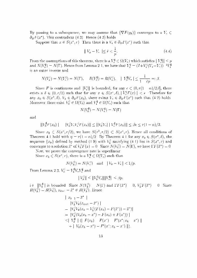
By passing to a subsequence, we may assume that frF (yk)g converges to a V� 2@BF (x�): This contradicts (4.3). Hence (4.2) holds.Suppose that x 2 S(x�; r). Then there is a V� 2 @BF (x�) such thatk Vx � V� k� �̂ < 1p: (4:4)From the assumptions of this theorem, there is a V ]� 2 (V�) which satis�es jjV ]� jj � pand N(V ]� ) = N(�): Hence from Lemma 2.1, we have that V ]x = (I+V ]� (Vx�V�))�1V ]�is an outer inverse andN(V ]x ) = N(V ]� ) = N(�); R(V ]x ) = R(V ]� ); k V ]xV� k� 11� �̂p =: �:Since F is continuous and kV ]� k is bounded, for any � 2 (0; r(1 � �)=2�], thereexists a � 2 (0; r=2) such that for any x 2 S(x�; �); jjV ]�F (x)jj < �. Therefore forany x0 2 S(x�; �), V0 2 @BF (x0), there exists V� 2 @BF (x�) such that (4.2) holds.Moreover there exist V ]0 2 (V0) and V ]� 2 (V�) such thatN(V ]0 ) = N(V ]� ) = N(�)and jjV ]0F (x0)jj = jjV ]0V�V ]� F (x0)jj � jjV ]0 V�jjjjV ]�F (x0)jj � �� � r(1� �)=2:Since x0 2 S(x�; r=2), we have S(x0; r=2) � S(x�; r): Hence all conditions ofTheorem 4.1 hold with � = r(1 � �)=2. By Theorem 4.1 for any x0 2 S(x�; �), thesequence fxkg de�ned by method (1.9) with V ]k satisfying (4.1) lies in S(x�; r) andconverges to a solution �x� of V ]0F (x) = 0. Since N(V ]0 ) = N(�), we have �F (�x�) = 0.Now, we prove the convergence rate is superlinear.Since xk 2 S(x�; r), there is a V ]� 2 (V�) such thatN(V ]k ) = N(V ]� ) and kVk � V�k < 1=p:From Lemma 2.3, V ]k = V ]kV�V ]� andkV ]k k � kV ]kV�kkV ]� k � �p;i.e. kV ]k k is bounded. Since N(V ]k ) = N(�) and �F (�x�) = 0, V ]kF (�x�) = 0. SinceR(V ]k ) = R(V ]0 ), xk+1 � �x� 2 R(V ]k ): Hencek xk+1 � �x� k= jjV ]kVk(xk+1 � �x�)jj= jjV ]kVk(xk � V ]k (F (xk)� F (�x�))� �x�)jj= jjV ]k (Vk(xk � �x�)� F (xk) + F (�x�))jj�k V ]k k (k F (xk)� F (�x�)� F 0(�x�; xk � �x�) k+ k Vk(xk � �x�)� F 0(�x�; xk � �x�) k):13

By (2.1) and Lemma 2.7, we havek F (x)� F (�x�)� F 0(�x�; x� �x�) k= o(k x� �x� k)and k Vx(x� �x�)� F 0(�x�; x� �x�) k= o(k x� �x� k):This implies k xk+1 � �x� k= o(k xk � �x� k):Hence method (1.9) converges to �x� superlinearly. 2Remark 4.4. Suppose that there is a V ]0 2 (V0) satisfying N(V ]0 ) = N(�). If thereis a Vk 2 @BF (xk) such that kV ]0 (Vk � V0)k < 1; (4:5)then V ]k = (I + V ]0 (Vk � V0))�1V ]0 is an outer inverse of Vk with N(V ]k ) = N(V ]0 ) =N(�) and R(V ]k ) = R(V ]0 ). Because of the nonsmoothness, we do not have the bene�tof a condition such as (3.4) to ensure (4.5). This is a major di�erence between smoothand nonsmooth equations.Remark 4.5. Superlinear convergence results in [31, 33] assume that all V� 2@BF (x�) are nonsingular. Under this assumption, x� is the unique solution of F (x) =0 in a neighbourhood N� of x� and it was only shown that kxk+1�x�k = o(kxk�x�k)for a sequence fxkg � N�. In singular case, the set of solutions may be locally amanifold of positive dimension. There is no neighbourhood N� of x� such thatmethod (1.9) converges to x� for any close starting point x0 2 N�. Condition (4.1) isimposed in Theorem 4.3 to guarantee the existence of a neighbourhood N� such thatmethod (1.9) converges to a solution of V ]0F (x) = 0 for any starting point x0 2 N�.The following corollary shows that condition (4.1) can be replaced by special choicesof starting points.Corollary 4.6. Let p be a positive number, � be an n�mmatrix and x� be a solutionof �F (x) = 0. Suppose that F is semismooth at x� and for all V� 2 @BF (x�); thereexists a V ]� 2 (V�), such that N(V ]� ) = N(�) and jjV ]� jj � p: Then method (1.9)with V ]k satisfying N(V ]k ) = N(�), R(V ]k ) = R(V ]0 ) and x0 2 R(V ]0 )+x� is convergentto x� superlinearly in a neighbourhood of x�.Proof. From the proof of Theorem 4.3, we have that there is a ball S(x�; �r), such thatfor any Vx 2 @BF (x); x 2 S(x�; �r), there is an outer inverse V ]x 2 (Vx) satisfyingN(V ]x ) = N(�) and jjV ]xV�jj � � for a V� 2 @BF (x�). Choosing x0 2 R(V ]0 ) + x�;we have xk+1 � x� 2 R(V ]k ) since R(V ]k ) = R(V ]0 ) and xk+1 � xk 2 R(V ]k ). Then we14

can show the superlinear convergence by the last part of the proof of Theorem 4.3(superlinear convergence). 2Remark 4.7. If we assume that m = n and all V� 2 @BF (x�) are nonsingular, thenwe can take � = I 2 Rn�n. Furthermore there is a neighbourhood N� of x�, suchthat for any x 2 N�, all Vx 2 @BF (x) are nonsingular. Then for any xk 2 N�, wecan take V ]k = V �1k which satis�es N(V ]k ) = N(�) = f0g, R(V ]k ) = R(V ]0 ) = Rnand xk 2 R(V ]0 ) + x�: Hence Theorem 4.3 and Corollary 4.6 generalize the localconvergence theorems given in [31, 33].Remark 4.8. In Theorem 4.3 and Corollary 4.6, V ]k should be chosen to satisfyN(V ]k ) = N(V ]0 ) and R(V ]k ) = R(V ]0 ) at each step of (1.9). There exists an outerinverse V ]k such that N(V ]k ) = N(V ]0 ) and R(V ]k ) = R(V ]0 ) if and only if N(V ]0 ) andR(VkV ]0 ) are complementary subspaces of Rm. If such an outer inverse exists, it isunique [2; p.62]. Now we give a method for numerical construction of such an outerinverse based on V ]0 and Vk. Let s =rank(V ]0 ) and rank(Vk) � s. Let U be a matrixwhose columns form a basis for R(V ]0 ), and let W be a matrix whose rows form abasis for the orthogonal complement of N(V ]0 ). Then WVkU is an s� s matrix withrank s, so it is invertible. Let V ]k := U(WVkU)�1W: Then V ]k is an outer inverse ofVk with N(V ]k ) = N(V ]0 ) and R(V ]k ) = R(V ]0 ).5. Examples and numerical experimentsIn this section we give methods for constructing outer inverses which are neededin the theorems and illustrate our results with three examples from nonlinear com-plementarity problems. The �rst example compares the theorems given in this paperwith earlier results. The second example shows how outer inverses apply while gener-alized inverses fail for Newton's method. The third example tests the methods (1.9)and (1.10) for problems with di�erent dimensions. The performance of algorithms isgiven by using Matlab 4.2c on a Sun 2000 workstation.5.1 Calculation of outer inversesMethods for constructing outer inverses of a given matrix or a linear operator aregiven in [2, 23, 24, 26]. For the case of an m� n matrix A with rank r > 0, we havea method using singular value decomposition (SVD). Let A = V�UT , where � isa diagonal matrix of the same size as A and with nonnegative diagonal elements indecreasing order, V and U arem�m and n�n orthogonal matrices, respectively. Let� > 0 be a computational error control, �]s=diag(v1; v2; :::; vs; 0; ::0) 2 Rn�m wheres �min(m;n) and vi = ( ��1i;i ; �i;i > j�j;0; otherwise:Then U�]sV T is an outer inverse of A. 15

As we know orthogonal-triangular decomposition (QR) is less expensive thanSVD. Here we give a new method to construct an outer inverse of A by using QR.Let A = QR be a factorization, where Q is an m�m orthogonal matrix, R is anm� n upper triangular matrix of the formR = R11 R120 0 !and R11 is an r � r matrix of rank r. Then A] = R]QT is an outer inverse of A,where R] = �R�111 00 0 ! ;and �R11 is an �r � �r matrix of rank �r � r.Remark 5.1 Outer inverses of a matrix A are more stable than the generalizedinverses when some singular values of A are close to zero, because we can choose �]and �R] such that their elements are bounded. For details of the perturbation analysisthat demonstrates stability of certain selections of outer inverses, see [22, 24, 26].Remark 5.2 For the smooth case, we need not construct an outer inverse at eachstep but only at the starting point. In practice, method (1.10) is implemented in thefollowing form: x1 = x0 � F 0(x0)]F (x0) and for k � 1, we let xk+1 = xk + d, whered is the unique solution of the linear system(I + F 0(x0)](F 0(xk)� F 0(x0)))d = �F 0(x0)]F (xk):Obviously, if m = n and F 0(xk) is invertible, then the method reduces to F 0(xk)d =�F (xk).5.2. Numerical examplesAs we stated in Section 1, a nonlinear complementarity problem (NCP) canbe formulated as a system of smooth equations by (1.7) and also as a system ofnonsmooth equations by (1.8). We can solve the smooth equations (1.7) by method(1.10) and the nonsmooth equations (1.8) by method (1.9). The singularity occursvery often in solving these two systems. It is interesting to see how to overcome thesingularity by methods (1.9) and (1.10) and Theorems 3.2 and 4.3.Example 1. We consider the following example [12]. Letf(x) = (1� x2; x1)T :The solution set of the associated NCP is W = f(0; �); j 0 � � � 1g. For eachx� 2 W , the Jacobian of F̂ de�ned by (1.7) isF̂ 0(x�) = �2(1� �) 0�2� 0 !16

which is singular. Hence previous local convergence theorems of Newton's method[9, 27, 34] are not applicable for this example. Now we apply Theorem 3.2 to thisproblem. We take x� = (0; 0:5). ThenF̂ 0(x�)] = a �1� aa �1� a ! 2 (F 0(x�))for any a 2 (�1;1). We take a = �1, L = 4, and p = 1. Then we can showthat there is a ball S(x�; r) with 0 < r < 0:5, such that jjF̂ 0(x�)]jj1 � p and for anyx 2 S(x�; r); jjF̂ 0(x)� F̂ 0(y)jj1 � Ljjx� yjj1. Hence all conditions of Theorem 3.2hold.Now we consider the nonsmooth equation (1.8). For any x� 2 W ,V� = 1 01 0 ! 2 @B ~F (x�):This implies F is not strongly BD-regular at all solutions in the sense of [31, 33].Hence the local convergence theorems in [31, 33] are not applicable for this example.However, we can choose an outer inverse asV ]� = 1 00 0 ! 2 (V�):Take x� = (0:0; 0:0). Then F is nonsmooth at x�. There is a ball S(x�; r) with0 < r < 0:5 such that for any x 2 S(x�; r), the generalized Jacobian isV (x) = 1 01 0 ! or V (x) = 1 00 1 ! :(For determination of a Vx 2 @BF (x) see [7, 31].)Hence we can take outer inverses V ]x = V ]� . Note that this is a linear com-plementarity problem, all conditions of Theorem 4.3 hold. Furthermore, for anyx0 = (�; �) 2 S(x�; r), x1 = x0 � V ]0 ~F (x0) = (0; �). If � � 0, then (0; �) 2 W .Example 2. The generalized inverse Ay of a matrix A is an outer inverse, but Aymay not be a good outer inverse for Newton's method. This example given by oneof the referees illustrates that conditions of Theorem 4.3 and Corollary 4.6 fail whenwe use generalized inverses. However these conditions hold for a number of outerinverses.Consider the piecewise linear equationF (x1; x2) = min(2x1 + x2 � 2;�2x1 + x2 � 2):17

The solution of F (x) = 0 is the union of the two rays:f(x1; x2) : x1 � 0; x2 = �2x1 + 2g [ f(x1; x2) : x1 � 0; x2 = 2x1 + 2g:This particular function, though nonsmooth, is well behaved in that its set of zerosis a 1-dimensional manifold, just as the solution of a linear equation in two variableis (usually) a line.For x1 � 0; let V = V1 = [2; 1] 2 @BF (x) andV y1 = " 2=51=5 # :Similarly for x1 > 0, let V = V2 = [�2; 1] 2 @BF (x),V y2 = " �2=51=5 # :It can be seen that for any staring point x0 = (x01; x02) such that x02 � �(1=2)x01 + 2and x02 � (1=2)x01 + 2, for instance x0 = (0; 0), the Newton's method de�ned byxk+1 = xk � V yi F (xk);where i = 1 if xk1 � 0 and i = 2 otherwise, converges linearly but not superlinearly to�x = (0; 2). The convergence is only linear, because although N(V y1 ) = N(V y2 ) = f0g,we have R(V y1 ) 6= R(V y2 ). We also see kV y2 (V1 � V2)k = 8=5 > 1. Thus Lemma 2.1cannot be applied; likewise (4.1) fails to hold in this case.Now we consider the use of outer inverses. It is easy to verify(V1) = f �� ! ; 2� + � = 1; j�j+ j�j 6= 0gand (V2) = f �� ! ;�2� + � = 1; j�j+ j�j 6= 0g:For any V ]2 2 (V2) with � < 1=4; kV ]2 (V1 � V2)k2 < 1: By Lemma 2.1, V ]1 =(I + V ]2 (V1 � V2))�1V ]2 is an outer inverse of V1 with N(V ]1 ) = N(V ]2 ) and R(V ]1 ) =R(V ]2 ). For instance, we choose V ]2 = �1=53=5 ! :Then V ]1 = (I + V ]2 (V1 � V2))�1V ]2 = �13 ! :18

Table 1n (1.10) for smooth eq. (1.9) for nonsmooth eq.k jjF (xk)]F (xk)jj cputime k jjV ]kF (xk)jj cputime50 13 2:83� 10�15 31.85 5 1:0� 10�16 3.97100 12 1:25� 10�14 144.15 4 1:0� 10�16 15.18200 8 3:10� 10�10 586.97 4 1:0� 10�16 137.20350 14 4:91� 10�14 4:92� 103 4 1:0� 10�16 577.95Furthermore for the starting point x0 = (0; 0),x1 = x0 � V ]1F (x0) = �26 ! :is a solution of F (x) = 0.Example 3. To compare methods (1.9) and (1.10), we randomly generate a NCPwith f(x) = Ax2 +Bx + c;where A and B are n� n matrices, c 2 Rn is a vector and x2 = (x2i ) 2 Rn.We �rst randomly generate singular matrices A and B, and a nonnegative vectorx� which has some zero elements. Then we choose c such that x� is a solution of aNCP with f(x) = Ax2+Bx+c: The problem is randomly generated but with knownsolution characteristic and singularity, so we can test the e�ciency of methods (1.9)and (1.10). Table 1 summarizes computational results with di�erent n. Also wechoose n = 100, x0 = x�+random vector and show jjF 0(xk)]F (xk)jj; jjV ]kF (xk)jj andconvergence rate jjF (xk+1)jj=jjxk+1 � xkjj in Figure 1.Concluding Remarks.In this paper, we discussed local convergence of Newton's method for singularsmooth and nonsmooth equations, respectively. These results generalize and extendearlier results on nonsingular smooth and nonsmooth equations. Singularity occursin many areas of optimization and numerical analysis. Pang-Gabriel [29] mentionedthat the singularity badly a�ected the convergence of the NE/SQP method for thenonlinear complementarity problem in a number of numerical examples. The resultsin this paper present a strategy to treat singularity and to guarantee convergence ofNewton's method and related iterative methods. Some of our results are also strongerthan earlier results in the nonsingular case since they involve weaker assumptions.AcknowledgementsWe are grateful to the referees for their constructive comments.19

0

1

2

3

4

5

1 2 3 4

iteration k

||V(x

)#F(

x)||

method (1.9)

0

0.5

1

1.5

2

1 2 3 4

iteration k

method(1.9)

conv

erge

nce

rate

0

20

40

60

80

0 5 10 15

iteration k

||F (

x)#F

(x)||

method (1.10)

0

200

400

600

0 5 10 15

iteration k

conv

erge

nce

rate

method (1.10)

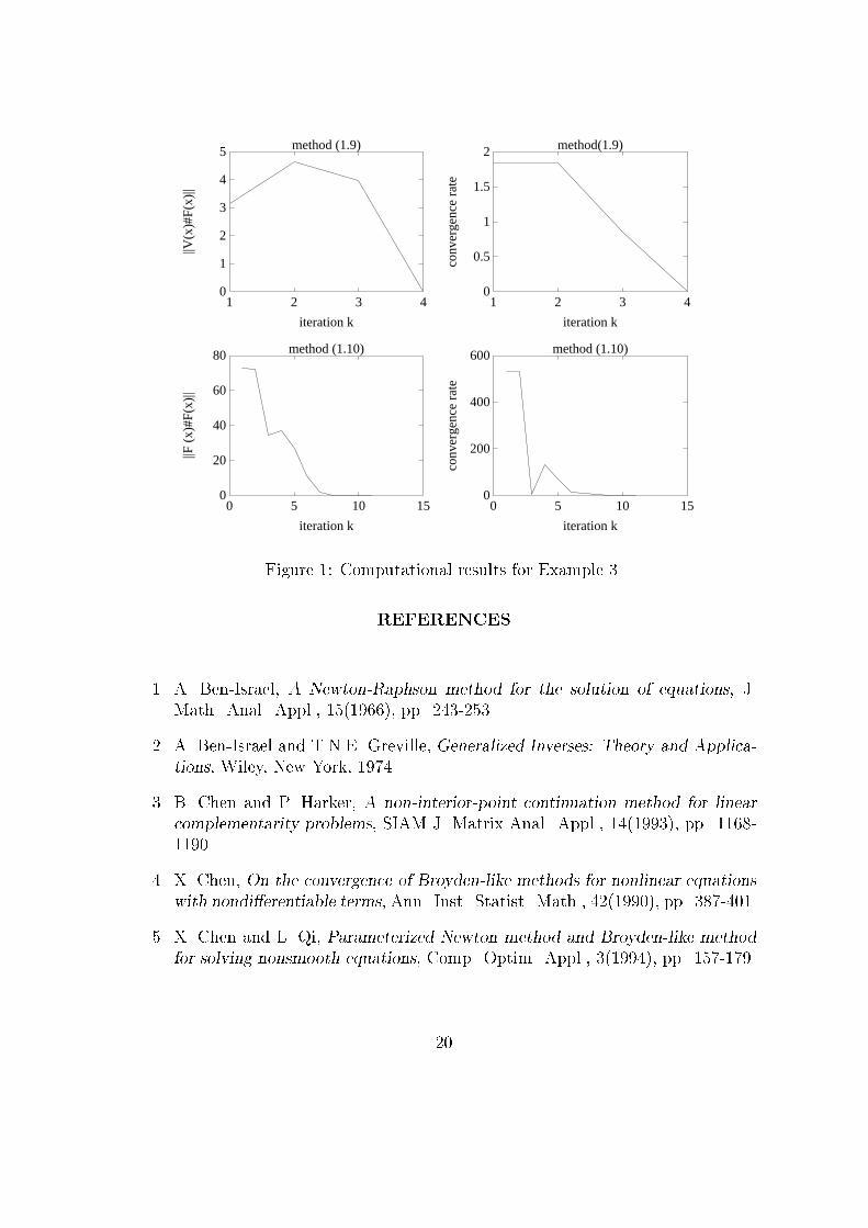
Figure 1: Computational results for Example 3.REFERENCES1. A. Ben-Israel, A Newton-Raphson method for the solution of equations, J.Math. Anal. Appl., 15(1966), pp. 243-253.2. A. Ben-Israel and T.N.E. Greville, Generalized Inverses: Theory and Applica-tions, Wiley, New York, 1974.3. B. Chen and P. Harker, A non-interior-point continuation method for linearcomplementarity problems, SIAM J. Matrix Anal. Appl., 14(1993), pp. 1168-1190.4. X. Chen, On the convergence of Broyden-like methods for nonlinear equationswith nondi�erentiable terms, Ann. Inst. Statist. Math., 42(1990), pp. 387-401.5. X. Chen and L. Qi, Parameterized Newton method and Broyden-like methodfor solving nonsmooth equations, Comp. Optim. Appl., 3(1994), pp. 157-179.20

6. X. Chen and T. Yamamoto, On the convergence of some quasi-Newton methodsfor nonlinear equations with nondi�erentiable operators, Computing, 48(1992),pp. 87-94.7. X. Chen and T. Yamamoto, Newton-like methods for solving underdeterminednonlinear equations, J. Comp. Appl. Math., 55(1995), pp. 311-324.8. F. H. Clarke, Optimization and Nonsmooth Analysis, John Wiley and Sons,New York, 1983.9. J. E. Dennis, Jr and R. B. Schnabel, Numerical Methods for UnconstrainedOptimization and Nonlinear Equations, Prentice-Hall, Englewood Cli�s, NJ,1983.10. P. Deu hard and G. Heindl, A�ne invariant convergence theorems for Newton'smethod and extensions to related methods, SIAM J. Numer. Anal., 16(1979),pp. 1-10.11. H. W. Engl and M. Z. Nashed, New extremal characterizations of generalizedinverses of linear operators, J. Math. Anal. Appl., 82(1981), pp. 566-586.12. M. Ferris and S. Lucidi, Globally convergent methods for nonlinear equations,Preprint of Computer Sciences Department, University of Wisconsin-Madison,# 1030 (1991).13. S. P. Han, J. S. Pang and N. Rangaraj, Globally convergent Newton methodsfor nonsmooth equations, Math. Oper. Res., 17(1992), pp. 586-607.14. W. M. H�au�ler, AKantorovich-type convergence analysis for the Gauss-Newtonmethod, Numer. Math., 48(1986), pp. 119-125.15. M. Heinkenschloss, C. T. Kelley and H. T. Tran, Fast algorithms for nonsmoothcompact �xed point problems, SIAM J. Numer. Anal., 29(1992), pp. 1769-1792.16. C. M. Ip and J. Kyparisis, Local convergence of quasi -Newton methods forB-di�erentiable equations, Math. Programming, 56(1992), pp. 71-89.17. M. Kojima and S. Shindo, Extensions of Newton and quasi-Newton methods tosystems of PC1 equations, J. Oper. Res. Soc. Japan, 29(1986), pp. 352-374.18. B. Kummer, Newton's method for non-di�erentiable functions, in J. Guddat, B.Bank, H. Hollatz, P. Kall, D. Klatte, B. Kummer, K. Lommatzsch, L. Tammer,M. Vlach and K. Zimmerman, eds., Advances in Mathematical Optimization,Akademi-Verlag, Berlin, 1988, pp. 114-125.21

19. O. L. Mangasarian, Equivalence of the complementarity problem to a systemof nonlinear equations, SIAM J. Appl. Math., 31(1976), pp. 89-92.20. O. L. Mangasarian and M. V. Solodov, Nonlinear complementarity as uncon-strained and constrained minimization, Math. Programming, 62(1993), pp.277-297.21. R. Mi�in, Semismooth and semiconvex functions in constrained optimization,SIAM J. Control Optim., 15(1977), pp. 191-207.22. R. H. Moore and M. Z. Nashed, Approximations to generalized inverses oflinear operators, SIAM J. Appl. Math., 27(1974), pp. 1-16.23. M. Z. Nashed, ed., Generalized Inverses and Applications, Academic Press,New York, 1976.24. M. Z. Nashed, Generalized inverse mapping theorems and related applicationsof generalized inverses, In: Nonlinear equations in abstract spaces (V. Laksh-mikantham, ed.), Academic Press, New York, 1978, pp. 217-252.25. M. Z. Nashed, Inner, outer, and generalized inverses in Banach and Hilbertspaces, Numer. Funct. Anal. Optim., 9(1987), pp. 261-325.26. M. Z. Nashed and X. Chen, Convergence of Newton-like methods for singularoperator equations using outer inverses, Numer. Math., 66(1993), pp. 235-257.27. J. M. Ortega and W. C. Rheinboldt, Iterative Solution of Nonlinear Equationsin Several Variables, Academic Press, New York, 1970.28. J-S. Pang, Newton's method for B-di�erentiable equations, Math. Oper. Res.,15(1990), pp. 311-341.29. J-S. Pang and S. A. Gabriel, NE/SQP: A robust algorithm for the nonlinearcomplementarity problem, Math. Programming, 60(1993), pp. 295-337.30. J-S. Pang and L. Qi, Nonsmooth equations: motivation and algorithms, SIAMJ. Optimization, 3(1993), pp. 443-465.31. L. Qi, Convergence analysis of some algorithms for solving nonsmooth equa-tions, Math. Oper. Res., 18(1993), pp. 227-244.32. L. Qi and X. Chen, A globally convergence successive approximation methodfor severely nonsmooth equations, SIAM J. Control Optim., 33(1995), pp. 402-418. 22

33. L. Qi and J. Sun, A nonsmooth version of Newton's method, Math. Program-ming, 58(1993), pp. 353-367.34. L. B. Rall, A note on the convergence of Newton's method, SIAM J. Numer.Anal., 1(1974), pp. 34-36.35. S. M. Robinson, Newton's method for a class of nonsmooth functions, Set-Valued Analysis, 2(1994), pp. 291-305.36. A. Shapiro, On concepts of directional di�erentiability, J. Optim. TheoryAppl., 66(1990), pp. 477-487.37. T. Yamamoto, On some convergence theorems for the Gauss-Newton methodfor solving nonlinear least squares problem, Proceedings of the Summer Sym-posium on Computation in Mathematical Sciences-Fusion of Symbolic and Nu-merical Computations, IIAS-SIS Fujitsu Ltd., 1987, pp. 94-103.38. T. Yamamoto, Uniqueness of the solution in a Kantorovich-type theorem ofH�au�ler for the Gauss-Newton method, Japan J. Appl. Math., 6(1989),pp.77-81.39. T. Yamamoto and X. Chen, Ball-convergence theorems and error estimatesfor certain iterative methods for nonlinear equations, Japan J. Appl. Math.,7(1990), pp. 131-143.40. N. Yamashita and M. Fukushima, Modi�ed Newton methods for solving semis-mooth reformulations of monotone complementarity problems, Math. Pro-gramming, to appear.

23