Forensic Estimation of Time Since Death: A Comparative Study Of Polynomial Regression And Modified...

Researchjournali’s Journal of Mathematics Vol. 2 | No. 6 July | 2015 ISSN 2349-5375

1

Akwasi Boahene

Department of Mathematics, Kwame Nkrumah

University of Science and Technology, Kumasi,

Ghana

Dr. E. Osei-Frimpong

Department of Mathematics, Kwame Nkrumah

University of Science and Technology, Kumasi,

Ghana

Forensic Estimation

Of Time Since Death:

A Comparative Study

Of Polynomial

Regression And

Modified Newton's

Models


2

ABSTRACT

Empirical studies have been made into the determination of Time Since Death (TSD).This study attempts to

briefly review most of the methods used to estimate TSD and concentrate on the development of a

Polynomial Regression Model (PRM) and a Modified Newton's Model (MNM) that accurately predicts TSD

and chose the most consistent, efficient and accurate estimator of TSD between the two. Such a model, when

accurately developed, will add to the security services scientific ways of predicting TSD, as well as, help in

civil and criminal cases. The study found out that the PRM best predicts TSD with an R2 of 99.87 %, given

the two secondary data obtained from the Journal of the Indian Academy of Forensic Medicine 2005 volume

27(3):170-176 and the Acta Morphologica 2006, volume 3(3):52-53.The MAPE, MAD and SSE of the two

models were also statistically tested and compared to that of the Actual Time Since Death (ATSD).The MNM

relied on the use of an iterative method, to determine the number of times, time (denoted t in hours) changes

over time for Rectal Temperature (RT) to coincide with the developed model of differential equation .The

calculation embodied several parameters /conditions that affect the cooling rate of dead bodies.

Keywords: Post-mortem Interval, Regression, Temperature plateau, Iterative Method, Algor Mortis,

Entomology, Homicide, Nomogram

1. INTRODUCTION

Several hundreds of thousand Murder/Homicide cases occur throughout Africa and the world. “International

homicide caused the deaths of almost half a million people (437,000) across the world in 2012. More than a

third of those (36%) occurred in the Americas, 31% in Africa and 28% in Asia, while Europe (5%) and

Oceania (0.3%), [20]. The huge number of murder cases gives credence to the need to determine a simple,

efficient, reliable and an easy to use mathematical/statistical model that can estimate the time of death of

murdered victims. The basic natural question asked by all during death is, "When did the victim die?”

Accurate estimation of the Time Since Death has several importance, be it in murder/accidental or natural

death. Proper solution to a civil matter can be arrived at through the use of an accurate estimated time of

death.

[7] puts; "in civil matters, time may be what determines whether or not an insurance policy was in effect or

void". For instance, if a client died hours before maturity of claims, it may not be paid. In other words, it helps

in the determination of an insurance claim. In criminal cases, the time of death may serve as a screening

process to either corroborate or refute or redefine suspects. Above all, it will serve a societal or family need of

satisfying the curiosity of friends and loved ones of the dead, as to TSD of victim.


3

Sadly, some security services in Ghana, Africa and parts of the world continue to rely on crude and

unscientific methods to determine/estimate the time of death, especially in homicide/murder cases.

Polynomial Regression Model (PRM) and Modified Newton's Models (MNM) are based on temperature

variations of the dead body. It follows the assumption of the Newton's Law of Cooling. They are just a tool

out of the myriad of tools within the reach of the forensic scientist to estimate TSD.

1.1 REVIEW OF SOME METHODS FOR ESTIMATING TIME SINCE DEATH(TSD)

Other measuring rods used to estimate time of death at the disposal of the Forensic Scientist are;

Livor mortis (Post Mortem lividity)

This is the resultant colour of a dead person's body due to pooling of blood and the work of gravity. At death,

the heart stops beating and blood vessels stop moving, halting blood circulation. Blood flows down the

inactive vessels into the lowest part of your body regardless of the body position. It is observed as a dark

purplish hue (shade of colour) onto the skin in which the blood had flown and pooled. Depending on the

extent of time, this colour can / will become permanently fixed on the body. Lividity will be present after 2-8

hours of death. But can be removed easily with pressure on affected area. Hence, if colour disappears, a

person probably died less than eight hours ago. If the colour remains person might have died beyond eight

hours.

Environmental factors such as temperature, accessories and clothing on dead body can affect livor

mortis.Environmental factors such as temperature, accessories and clothing on dead body can affect livor

mortis. Extremely cold temperature slows down livor mortis and vice versa. Belts, wrist watches and clothing

can also externally constrict blood passage slowing down livor mortis, [15].

Rigor Mortis

[6], defined Rigor Mortis as the generalized stiffening of the skeletal and smooth muscles of the body

following death. [15], also described it as the extremely stiffening of the body‟s muscles due to the build-up

of calcium in muscle fibre and the inability to remove excess calcium. Rigor mortis begins after two hours of

death, starting from the head and slowly progressing to the feet. After 12 hours the dead body would be at its

most rigor state. After 36 – 48 hours, the body would resume the soft dead body status. Process of rigor

mortis depends on temperature, body weight and body temperature and sun exposure. It is faster in hotter

bodies and slower in cooler bodies, [15].

The colour of the eye

Cloudiness of the cornea will appear within a few hours to 24 hours, depending on the degree of closure of

the eyelids, environmental temperature, humidity, and air movement. It is not recommended that you attempt

to use cloudiness of the cornea for determination of post-mortem intervals due to the multitude of factors,


4

which affect it, [6]. The transparency of the Cornea is very variable. [11], claimed that, the variability of the

Cornea is less than other methods of estimating PMI. His analysis of 238 autopsies' cornea revealed that,

transparency. They concluded that changes of the Cornea occurs more in warm and moist weather than in

warm and dry weather and cold and moist respectively and least in cold and dry weather. That changes of the

Cornea occurs more in warm and moist weather than in warm and dry weather and cold and moist

respectively and least in cold and dry weather.

Forensic Entomology

Forensic Entomology is the study of insects found at the crime scene. A pathologist is able to establish a more

accurate time scale depending on which insect are found on the body and what they are at in their life cycle,

[5]. Forensic entomology works in death scene investigation because insects are defined by certain

characteristics and follows a predictable pattern of development, [21]. Arthropods (invertebrate animals with

joint limbs) are most important in forensic entomology because they eat dead vertebrate bodies, including

man. One of the first groups of insects that arrive on a dead vertebrate is usually the blowflies (Dipteria,

calliphoridae). The female blowflies oviposit (lay eggs) on dead body within few hours.

(www.cienciaforense.com/pages/entomology/overview.htm). Blowflies and insects go through four

developmental stages called complete metamorphosis. A careful or correct calculation of these stages of

development of insects as well as other creatures present at a crime scene can lead to the estimation of the

time since death.

The following table of approximation of the time of death, using insects present and stages of dead body is

developed from the following article; [22] and [3].

Approximate time of death Appearance of body/stage Insects present

Few minutes – 3 days Fresh stage Just like sleeping. Last

until body bloats

Blowflies and flesh flies arrive

minutes after death. Begins to lay

eggs/deposit maggot. Maggots

begin to feed on body tissues. Ants

begin arriving.

4 – 7 days Bloated stage Body becomes visibly

inflated, especially abdomen. Colour

change and odour of putrefaction is

noticeable.

Blowflies, houseflies, flesh fly,

maggot, beetles, ants and other

creatures feed on maggot.

8 – 18 days Decay active stage Carcass deflates.

Has wet appearance and a strong

odour of putrefaction.

Ants, cockroaches, beetles and

flies.

19 – 30 days Advanced decay/post decay stage.

Most flesh remove from carcass.

Strong odour of decomposition being

to fade

Adult skin beetle and mite arrives

at carcass. Larval stages are absent.

Instar calliphorid being to leave

carcass

31 days and over Dry decay

Bones, hair and portions of skin stench

is no longer powerful

Centipedes, isopods, snails and

cockroaches.


5

The above table gives a general decomposition model of a dead body. However, factors such as temperature

(slow decomposition at cold periods and vice versa), drug present in body at death, clothing and access to

dead body can affect rate of decomposition.

[8], postulated that insects are frequently the first organisms to arrive at a dead body. That, their activities

begin a biological clock that will allow for an estimation of the post mortem interval (PMI).Five -5- stages of

decomposition (fresh, bloated, decay post-decay and skeletal) are suggested as reference points in the

decomposition process. Factors that may delay invasion of the remains by arthropods or alter developmental

patterns, such as presence of drug and toxins, wrapping of body and climate were discussed by [8]. [9], saw

entomology as the application of knowledge of insects during investigation of crimes or other legal matters.

His study of Insect evidence or presence revealed that insects of the form of blow flies in their different stages

of development are found on fresh and decaying corpses. Beetles were found on skeletonised bodies.

Henssge Nomogram Method

The Nomogram method is based on a formula which follows the sigmoid shape of the cooling curve.The

formula contains two exponential constant parts. The first represent the Post Mortem Plateau and the second

constant shows the exponential drop of temperature after the Plateau according to the Newton‟s law of

cooling, described by [16]. A widely used Nomogram for a forensic time of death determination is the one

published by Henssge in 1981. He presented a simplified method to determine the Newton cooling

coefficient, by finding out statistical figures of the deviation between calculated and real death times for

cooling under standardized conditions (e.g. ambient temperature of below 230C and above 23

0C). His

Nomogram is in two folds; one for ambient temperature above 230C and one for ambient temperature below

230 C.

Based on conventional calculations such as those of; De Saram and Marshall as well as backed by a great

volume of experimental data, Henssge has produced a method which can be carried out either by a simple

computer program or a Nomogram. The results are given within different ranges of error, with a 95 %

probability of the true time of death falling within this ranges. The ranges vary from 2.8 hours each side at a

best estimate to 7 hours at worst, [18].

To read off the time of death, connect the rectal and ambient temperature on the Nomogram with a straight

line, so that it crosses the diagonal line on the Nomogram. A second straight line is then drawn from the

centre of the circle at the bottom left of the diagram to intersect the diagonal line and the initial line drawn on

the Nomogram. The second line crosses the semi-circles of the body weight and that of the outermost semi-

circle. The estimated time of death is read off .The outermost intersection gives the margin of error at 95%.

For instance, given a body temperature of 28.80

C, ambient temperature of 210

C and body weight of 83 kg,


6

with an ATSD of 13 hours. Then, the estimated time of death becomes; 16 ± 2.8 hours. The death occurred

between 13.2 and 18.6 hours, before the measurement with a 95 % reliability level.

Henssge Nomogram for ambient temperature up to

Source: Pellini, 2011

Algor Mortis

The Algor Mortis is the bases of all the temperature based models for the estimation of the TSD. Extensive

research has shown that, the human body temperature is averagely above that of the ambient (atmospheric)

temperature. This temperature reduces in the body after death. This reduction in the body is called Algor

mortis. Unlike forensic entomology, Algor Mortis is most effective during the first 24 hours of death. Its

effectiveness fades as actual time since death increases. Post Mortem interval / cooling does not begin

immediately after death, it stays constant for a period before reducing. This initial lag in temperature, termed

as Temperature Plateau was defined by [17], as the period after death where, the body does not cool at all and

may even rise.


7

Source: HenBgea and Madea, 2004

2. METHODOLOGY

An address of the Polynomial regression models (PRM) and the Modified Newton‟s Model (MNM) will be

made. Both models are examples of temperature based models used in the estimation of TSD.

2.1 POLYNOMIAL REGRESSION MODEL

2.1.1 REGRESSION

It is a statistical technique to determine the linear relationship between two or more variables. They are

primarily used for prediction and causal inference. In its simplest (bivariate) form, regression shows the

relationship between one independent Variable (X) and a dependent Variable (Y) as in the formula below;

(1)

Where,

the intercept parameter

the amount of variation not predicted by the slope and intercept) [2].


8

2.1.2 A POLYNOMIAL REGRESSION MODEL (PRM)

Polynomial Regression Model can be said to be a form of a regression that fits a non-linear relationship

between independent observed variables say, and a resultant dependent variables , where, ' ' is

expressed as a Vandermonde matrix of degree. PRM are considered as both Linear and multiple

regression models.

2.1.3 ASSUMPTIONS UNDER THE POLYNOMIAL REGRESSION MODEL

Just as a linear regression assumes that, the relationship you are fitting a straight line to, is linear,

polynomial regression assumes that you are fitting the appropriate kind of curve to your data. It assumes

that data points are independent.

The variable is normally distributed and homoscedastic for each value of . [14].

The behaviour of a dependent variable y can be explained by a linear, or curvilinear, additive

relationship between the dependent variable and a set of „K‟ independent variables (X j, j = 1... K).

The relationship between the dependent variable y and any independent variable x j are independent of

each other and

The error term (ε) are independent, normally distributed with mean zero and a constant variance

/standard deviation. In other words, ε ~ (0, σ 2).

2.1.4 BUILDING THE POLYNOMIAL REGRESSION MODEL

Order of the Model

The order (K) of polynomial models should be kept as low as possible. [4], advised that, higher-order

polynomials (K > 2) should be avoided unless they can be justified for reasons outside the data. It is

extensively known that the cooling/heating of the rectal temperature of a dead body follows a sigmoid (S)

Shape, hence, cubic. Supported by [10]; "The curve of the cooling (of a dead body) is sigmoid in pattern".

Polynomial Regression Model in Matrix

Let X be an n X k matrix with observations on K independent variables for a total of n observations. As

our model contains a constant term, the first columns in the X matrix will contain only ones.

Let Y be an n X 1} vector of observations on the dependent variable.

Let ε be an n X 1 vector of disturbances or errors.

Let β be a k + 1 vector of unknown population parameters that we want to estimate.

Then the realization of this relationship in a general regression models can be written as a system of equations

as follows;


9

=

+

The general regression model can be written as , in matrix. Therefore, the expected value

of , gives; , [1]. Using the Least Square Method in Matrix, we find the estimators , that

minimizes the sum of squares residuals

, with a vector of residual of form; .

Hence,

The Sum of Squares Residual can be expressed as;

=

Hence,

( ) (2)

Expanding

= y y – X y – y X + X X

= y y -2 X y + X X (3)

Using the identity that the transpose of a scalar is a scalar;

= ( ) = X y , and minimizing with respect to

= -2 X y + 2 X X = 0 (4)

Hence, X X = X y

Multiply through the equation by (X X)-1

with the assumption that, the inverse of the matrix exists, gives;

= (X X)-1

X y

The modelled Polynomial Regression (PRM) becomes;

= (5)


10

Replacing the R.H.S of (5) by the hat matrix (H), gives; . Where H, is idempotent (H2

= H X H = H)

and symmetric (H = H T).

2.1.5 APPLICATION OF DATA TO THE PRM

If we replace the X matrix by our observed rectal temperatures to form a Vandermonde matrix of degree 3,

and solving the expression for , [(X'X)-1

X'Y], we will get the following estimates of .

X =

Y =

X X =

X Y =

, = =

=

Hence, the 3rd

degree Polynomial Regression Model from our data becomes;

= + -0.001259 (6)

2.1.6 VALIDITY AND PREDICTABILITY OF THE MODEL

The following R summary and Anova outputs for the 3rd

degree Polynomial Regression Model aids in

analysing and checking the validity and predictability of the Model.

R Output Summary

Coefficients Estimates( ) Standard

Error

t-Value p-Value

Intercept 963.959713 124.3 7.738 0.0000289

X -30.894845 4.46 -6.915 0.0000695

X2

0.338438 0.05323 6.358 0.000132

X3

-0.001259 0.0002103 -5.986 0.000206

R2

0.9987

R2 Adj. 0.9982


11

Residual

Standard

Error

0.3267

Source: author

Analysis of Variance Table

Degree of

Freedom(DF)

Sum of

square

Mean square F-value P-value

3 727.04 242.346 2270.7 2.846 e-13

Residuals 9 0.96 0.107

Source: author

The R2 squared and Adjusted R

2 squared (i.e. the percentage of variance in the dependent variable that

can be explained by the predictors) are 99.87% and 99.82 % respectively. This shows that the

Polynomial Regression Model is an accurate fit or predictor of the Time since Death (TSD).

The Standard Error of the estimate (cubic estimate) is very small, 0.0002103. Hence, the errors of the

residual tends to be closer to the mean. This implies that, the model predicts well the dependent

variable.

Testing for a cubic relationship between the TSD and RT, we test the H0:β3 = 0 against H1: β3 ≠ 0.

Significant level (α = 0.05), P-value of the coefficient of the X3, is 0.000206. As the p-value (0.0002103)

< α (0.05), we reject the H0 in favour of H1 and conclude that, there is a cubic relationship between TSD

and RT at 95% level of significance.

The Mean Square Error (MSE) for our estimate is (SSE/degree of freedom) = 0.107. Hence, size of the

errors in the regression is very small. In other words it shows that the regression fits the data very well.

Again, the Mean Absolute Percentage Error (MAPE), calculated as ;

MAPE=

(7)

Gives 2.7225 ≈ 2.72%. Since it lies less than 10% it shows that the PRM is an Excellent-Accurate forecaster

of the TSD.

The test statistics for calculating the Confidence Interval (I) and Predictive interval (PI) for the Regression

Models are;

(8)

And

(9)

Respectively.


12

Where, n is the total number of observation (13), is the predicted value (estimated TSD), SE, is the standard

deviation of the error term (0.3267), is the mean of the RT (81.99) and XA is the actual time TSD we

wanted estimate (10) .

Given a rectal temperature of . (Check Appendix)

= + -0.001259 =9.76 hours

which corresponds with the actual time of death of case 5.

The t-value associated with (1-α) confidence, = = 2.228

A 95% C.I and P.I are as follows;

n = 13, s = 0.2374, and = 12.2542

C.I at 95% level of significance for = 9.76 ± 2.228*0.3267 * 1.03786729761

=9.76±0.2019569828

Hence we are 95% confident that the, the prediction of will fall within

(9.55804, 9.96196).

Also, the P.I at 95% level of significance for = 9.76 ± 2.228 x 0.3267 x 1.03786729761

= 9.76 ± 0.7554507364

= (9.00455, 10.51545).

We are 95% confident that the estimate for a RT of 85.330 F, would be contained in the interval

(9.00455, 10.51545).

Summary of Validity of the PRM

Calc.

Stats

Value Implication on the PRM

R2

99.87 Accurate predictor of TSD.

SE 0.0002103 PRM is a good predictor of the independent variable.

MSE 0.107 Small Error in the Regression. Fits data very well.

MAPE 2.72 Excellent and Accurate Forecaster of TSD.


13

2.2 NEWTON’S MODEL

Mathematically the Newton‟s law of cooling is defined as follows;

a (10)

Where;

T, is the temperature of a cooling object, in our case a dead body.

t, is the time in hours since the first measurement of the body.

Ta, is the ambient temperature.

, is the constant of proportionality between the ambient and body temperature.

Solving the Above equation gives the following model;

T (t) = Ta +T0 - Ta (11)

Which is the well Known Newton's Model. It assumes a constant Ambient Temperature and does not consider

a lot of parameters in its computation. This makes them largely inaccurate in estimating TSD. [13], came to

the realization that dead bodies do not correspond perfectly to the Newton's Law of Cooling, especially,

during the initial stages of death. [13], after graphing the general shape of the curve that describes the

temperature of a cooling body added a “correcting factor” to the Newton‟s Law to represent the plateau. The

said correction factor is exponential in form and decays with time. The expression for this function is (Ce-pt

)

the differential equation for the deceased body then becomes;

=-K (T-Ta) + c (12)


14

Where K and P are cooling rate constants for the cooling factor and Plateau (indicated by the clothed states),

all other parameter denote the same meaning as in the Newton‟s model above.

Writing the above equation in standard form as;

+ P (t) y = Q (t) (13)

, where P (t) = K

Then the Integrating Factor (IF) becomes IF = =

Multiplying through equation 12, by the IF gives;

(14)

a

(15)

But, simplifying the L.H.S, using the following product rule of differentiation,

U(x)

+V(x)

=

(u(x) v(x)) (16)

, gives;

a

(17)

Integrating both sides w.r.t. t becomes;

(18)

(19)

Multiply equation 19, by,

gives;

T = Ta

+

T (t) = Ta +

(20)

if t = 0 , T(t)=0=T0 , then; T0 = Ta +

+ A .

Hence, A = T0 -Ta -

(21)

From 12, if t = 0;

(22)


15

Put equations 21 and 22 into equation 20 and simplify further

T (t) = Ta+

+ (T0 -Ta) (1-

)

T (t) = Ta+ (T0 -Ta) ((

+ (1-

) ) (23)

T (t) = Ta+ (T0 -Ta) (

) + ) (24)

Which is the final Modified Newton's Model (MNM) for estimating time since death.

From [12],

The rate constant of the Newton‟s model (K) is given as; K = Size Factor (SF) * 0.0006125- 0.05375

Where, SF = 0.8 *

While the rate constant for the plateau (P) is given as 0.3 for clothed body and 0.4 for nude bodies.

An Iterative method that iterates the number of times time (denoted t in hours) changes over time for Rectal

Temperature (RT), (T(t)) to coincide with the developed model of differential equation 22, embodying several

parameters /conditions that affect the cooling of dead body is used to estimate the TSD.

3. RESULTS

Two secondary data obtained from the Journal of the Indian Academy of Forensic Medicine 2005 volume

27(3):170-176 and the Acta Morphologica 2006, volume 3(3):52-53 (Macedonia Association of Anatomists

and Morphologists), were used for this paper. The first data presents Rectal Temperature of 418 adult subjects

aged between 18 and 60 years who died through accident at the Tropical region of Chandigarh (India), [19],

was used to develop the PRM. While the second data which presented analysis of 50 dead bodies with KTSD

were used to validate the predictability of the two models.

The following table presents the results obtained using the two models, PRM and the MNM‟s and the Actual

or Known Time Since Death (KTSD).

Estimated Results of TSD Using the PRM and MNM

CASE SEX Ta oC/

0F RT

OC/

OF Weight

(kg)

CLOTHED ATSD PRME MNME

1 M 17/34 34.9/94.82 65 + 4 4.04 2.76

2 F 22/62.6 34.4/93.92 65 + 4 4.62 4.48

3 M 19.3/66.74 35.1/95.18 78 + 4 3.80 4.28

4 F 22.5/72.5 34.7/94.46 75 - 4 4.28 4.85

5 M 22.4/72.32 35.9/96.62 65 - 4 2.76 2.96

6 M 24/75.2 33/91.4 75 - 5 6.16 7.93

7 M 21/69.8 36.5/97.7 80 - 5 1.91 2.06


16

8 M 22.4/72.32 32.8/91.04 80 - 6 6.36 7.7

9 F 22/62.6 32.2/89.96 58 - 6 6.98 5.82

10 M 21/69.8 34/93.2 75 - 6 5.08 5.41

11 M 16.5/61.7 33.2/91.76 60 + 6 5.95 5.47

12 M 20/68 33/91.4 78 - 6 6.16 6.47

13 M 24.5/76.10 34.1/93.39 70 + 6 4.97 6.86

14 M 21/69.8 32/89.6 57 - 7 7.19 7.15

15 M 16/60.8 30.6/87.08 80 + 7 8.64 8.79

16 M 21.3/70.34 32.5/90.5 80 + 7 6.93 8.42

17 M 24/75.2 33/91.4 78 + 7 6,16 8.85

18 M 24/75.2 33.9/93.02 82 + 7 5.19 7.44

19 M 24/75.2 33.8/92.84 84 + 7 5.30 7.69

20 M 22.5/72.5 33/91.4 70 + 7 6.16 7.76

21 M 30/86 33.4/95.72 75 + 7 3.42 7.17

22 M 21/69.8 32/89.6 72 - 8 7.19 7.86

23 M 21.2/70.16 32.4/90.32 55 - 8 6.78 6.66

24 M 21/69.8 32.6/90.68 85 - 8 6.57 7.60

25 M 24/75.2 32/89.6 50 - 9 7.19 8.16

26 M 19/66.2 31.6/88.88 78 + 10 7.60 8.61

27 M 23/73.4 30.9/87.62 80 + 10 8.32 12.14

28 M 15.7/60.26 27.2/80.96 75 + 12 12.92 12.38

29 M 24/75.2 29.6/85.28 80 + 13 9.75 16.23

30 M 21/69.8 .8/83.84 83 - 13 10.71 13.64

31 M 16.5/61.7 28.1/82.58 80 - 13 11.62 11.14

32 M 18/64.4 28.4/83.2 75 - 14 11.27 11.23

33 F 20.6/69.08 27.2/80.96 54 - 14 11.92 13.42

34 F 20/68 27.5/81.5 45 - 14 12.47 11.42

35 M 23/73.4 27/80.6 75 - 15 13.23 21.55

36 M 24.4/75.92 25.9/78.62 76 + 15 15.11 33.06

37 M 23.6/74.48 24.1/75.38 75 - 15 18.90 51.95

38 M 20/68 24.5/76.1 80 - 15 17.97 23.35

39 M 21/69.8 24/75.2 73 + 16 19.15 27.07

40 M 23/73.4 23.5/74.3 95 + 17 20.41 58.26

41 M 19/66.2 23/73.4 80 + 19 21.77 25.91

42 M 22/71.6 23.3/73.94 95 + 19 20.94 43.85

43 M 22/71.6 23.3/74.3 85 + 19 21.77 45.04

44 M 17/62.6 23/73.4 75 + 20 22.63 21.53

45 M 17/62.6 22.7/72.86 70 + 20 23.22 21.30

46 M 17/62.6 22.5/72.5 76 + 20 23.22 22.19

47 F 20.6/69.08 22/71.6 65 - 21 24.6 34.56

48 M 21/69.8 21.6/70.88 73 + 22 26.11 49.23

49 M 20/68 21.3/70.34 80 + 24 27.15 41.49

50 M 21/69.8 21.8/71.24 60 - 24 25.44 39.65

Source: Acta Morphologica 2006, volume 3(3):52-53


17

Comparing the means of the PRME and MNME and that of the KTSD at a 95% significant level

revealed that; Preliminary analysis of the result(s) churned out from the two models reveals that, there

are no difference between the estimates of PRM and KTSD. However, there existed a difference

between estimates of MNM and KTSD except without the outliers.

The parametric statistic of the population, (KTSD) variance (σ2).

(24)

Hence, The Standard Deviation is =5.97 and μ = 11.38. Since σ2 is known and N > 30 we use the Z test

statistic of

(25)

And the Z critical is Z0.025 = ± 1.96

0 1 2 3 4 5 6 7 8 9 101112131415161718192021222324252627282930313233343536373839404142434445464748495002468

1012141618202224262830323436384042444648505254565860

Number of Cases

Tim

e S

ince D

eath

(H

ours

)

Plots of Actual/Known TSD , PRME and MNME

ATSDPRMEMNME

0 2 4 6 8 10 12 14 16 18 20 22 24 26 28 30 32 34 36 38 40 42 44 46 48 50 520

5

10

15

20

25

30

35

40

45

50

55

60

NUMBER OF CASES

TIM

E S

INC

E D

EA

TH

BAR CHART FOR THE ATSD,PRME AND MNM

ATSDPRMEMNME


18

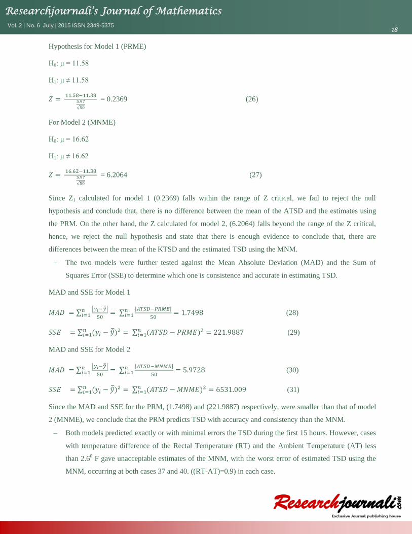
Hypothesis for Model 1 (PRME)

H0: μ = 11.58

H1: μ ≠ 11.58

= 0.2369 (26)

For Model 2 (MNME)

H0: μ = 16.62

H1: μ ≠ 16.62

= 6.2064 (27)

Since Z1 calculated for model 1 (0.2369) falls within the range of Z critical, we fail to reject the null

hypothesis and conclude that, there is no difference between the mean of the ATSD and the estimates using

the PRM. On the other hand, the Z calculated for model 2, (6.2064) falls beyond the range of the Z critical,

hence, we reject the null hypothesis and state that there is enough evidence to conclude that, there are

differences between the mean of the KTSD and the estimated TSD using the MNM.

The two models were further tested against the Mean Absolute Deviation (MAD) and the Sum of

Squares Error (SSE) to determine which one is consistence and accurate in estimating TSD.

MAD and SSE for Model 1

(28)

(29)

MAD and SSE for Model 2

(30)

(31)

Since the MAD and SSE for the PRM, (1.7498) and (221.9887) respectively, were smaller than that of model

2 (MNME), we conclude that the PRM predicts TSD with accuracy and consistency than the MNM.

Both models predicted exactly or with minimal errors the TSD during the first 15 hours. However, cases

with temperature difference of the Rectal Temperature (RT) and the Ambient Temperature (AT) less

than 2.60 F gave unacceptable estimates of the MNM, with the worst error of estimated TSD using the

MNM, occurring at both cases 37 and 40. ((RT-AT)=0.9) in each case.


19

The PRME on the other hand stayed within range, predicting TSD throughout the fifty (50) cases with

very little discrepancies.

3.1 SUMMARY OF COMPARATIVE VALIDATION OF PRME AND MNME

Calc.

Stats

PRME MNME Implication On Estimated Results.

MAD 1.7498 5.9728 PRM is an accurate predictor of TSD than MNM

SSE 221.9887 6531.009 PRM is a consistent predictor of TSD than MNM

4. DISCUSSION AND CONCLUSION

The study achieved all of its aims including determining the best model for estimating TSD between the PRM

and the MNM. PRM estimated TSD better with little or no discrepancies. The MNM was also good in

determining the TSD for the first 15 hours after death (Where (RT-AT) >2.6 0 F)

Further investigations revealed that, the MNM will produce estimates of TSD having larger / unacceptable

errors, if the difference between the Rectal Temperature (RT) and Ambient Temperature (AT) is between (0.1

and 5 0 F).

Hence, based on the analysis of the results, I conclude that the Polynomial Regression Model (PRM) is the

best estimator of Time Since Death in all circumstances of death relative the Modified Newton's Model.

5. REFERENCES

[1] Nathaniel Beck. Ols in matrix form. http://weber.ucsd.edu/nbeck, 2001.

[2] Dan Campbell and Sherlock Campbell. Introduction to regression and data analysis. Stat Lab Workshop, 2008.

[3] Lisa Carloye and Stephen Bambara. Crime solving insects. North Carolina Cooperative Extension Service, 2006.

[4] Ray-Bing Chen. Polynomial regression models. Institute of Statistics National University of Kaohsiung, 2014.

[5] Jack Claridge. Estimating the time of death. Explore Forensic, 2015.

[6] William A. Cox. Early postmortem changes and time of death. 2009.

[7] Vernon J. Geberth. Estimating the time of death in practical homicide investigations. Law and Order Magazine, 55, 2006.

[8] M.L. Goff. Estimation of postmortem interval using arthropod development and successional patterns. Forensic Sci Rev 5, pages

81{94, 1993.

[9] Parmod Kumar Goyal. An entomological study to determine the time since death in cases of decomposed bodies. J Indian Acad

Forensic Med., 34, 2012. 20

[10] R.N. Kamakar. Forensic Medicine and Toxicology. 3rd Edition. Bimal Kumar Dhur of Academic Publishers, 2010.

[11] Binay Kumar, Vinita Kumari, Tulsi Mahto, Ashok Sharma, and Aman Kumar. Determination of time elapsed since death from

the status of transparency of cornea in Ranchi in di_erent weathers. J Indian Academy of Forensic Medicine. 34, 2012.

[12] N. Lynnerup. A cumputer program for the estimation of time of death. Journal of Forensic Science, JFSCA, 38(4):816 to 820,

1993.

[13] T.K Marshall and F.E Hoare. Estimating the time of death: the rectal cooling after death and its mathematical expression. Journal

of Forensic Sciences, 7, 1962.


20

[14] J.M. McDonald. Handbook of Biological statistics. Sparky House, 2014.

[15] T. Norman. 4-ways-to-determine-time-of-death-in- a -dead-person, January 2012.

[16] V. Poposka, A. Gutevska, A. Stankov G. Pavlovski, Z. Jakovski, and B. Janeska. Estimation of time since death by using

algorithm in early postmortem period. Global Journal of Medical research Interdisciplinary, 13, 2013.

[17] Harry Rainy. On the cooling of dead bodies as indicating the length of time since death. Glasgow Medical Journal, 1868.

[18] P. Saukko and B. Knight. Knight's forensic pathology. Arnold Publishers, 3rd Ed, 2004.

[19] Dr. Dalbir Singh, Dr. Suresh Kumar Sharma, Dr. Indar Jit Dewan, Dr. Y.S. Bansal, Dr. Vishal, and Mr. Avadh Naresh Pandeya.

Polynomial regression model to estimate time since death in adults from rectal temperature in Chandigarh zone of northwest India.

Journal of the Indian Academy of Forensic Medicine, 27:170{175, 2005}.

[20] UNODC. UNODC Global Study on Homicide 2013. United Nations Publications, 2014.

[21] Dick Warrington. Crime scene bugs. Forensic Magazine, 2010.

[22] Wikepedia. Decomposition. Wikipedia, The Free Encyclopedia, page 627010363, 2014.

APPENDIX

Mat lab code for Iteration

data = [rectal , ambient, weight, clothed state ]

extimated_tn = zeros (size (data,1)) ;

For i =1: size (data, 1)

t = 0.001;

T0 = 98.96;

T = data (i, 1);

Ta = data (i, 2);

W = data (i, 3);

threshold = abs (T * 0.0001);

BSA = 0.1173 * (W^ 0.6466);

SF = 0.8 * BSA*10000 / W;

k = SF * 0.0006125 - 0.05375;

p = data (i, 4);

loop = 1;

while loop

tv = Ta + (To - Ta)* (exp(-k * t) + (k/(k-p))*((exp(-p*t))-(exp(- k*t))));

ans = abs( T - tv);

if ans <= threshold

estimated_t(i) = t;

loop = 0;

else

t = t + 0.001;

end

end

end

estimated_t'


21

Data for PRM

TSD(Hrs.) 2 4 6 8 10 12 14 16 18 20 22 24 26

RT (0 F) 98.04 95.07 91.60 88.33 85.33 82.60 80.16 77.96 76.03 74.39 73.05 72.05 71.31

Source: JIAFM 2005 volume 27(3):170-176

Acknowledgement

The author wants to express sincerest thanks to John Torgbui Galley, Daniel Molley and Matilda Owusu Boakye for their support and

contributions in this paper.

Forensic Estimation of Time Since Death: A Comparative Study Of Polynomial Regression And Modified...

Documents

Transcript of Forensic Estimation of Time Since Death: A Comparative Study Of Polynomial Regression And Modified...