Newton's method applied to two quadratic equations inC

Newton’s method applied to

two quadratic equations in C2

viewed as a global dynamical system

John H. Hubbard and Peter Papadopol

In this paper, we will study Newton’s method for solving two simultaneous quadratic equationsin two variables.

In one dimension, if F is a polynomial, the Newton mapping is a rational function and we canapply the now rather well developed theory of one-dimensional complex analytic dynamics. Thesubject is far from completely understood, but much progress has been made, particularly by J.Head, Tan Lei, and M. Shishikura. More recently, [HSS] give precise results on how to find all theroots of a polynomial, based on the topology and complex analysis of the basins.

Presumably, there is no need to motivate a study of Newton’s method, in one or several variables.The algorithm is of immense importance, and understanding its behavior is of obvious interest. Itis perhaps harder to motivate the case of two simultaneous quadratic equations in two variables,but this is the simplest non-degenerate case.

The classical theory, due to Ostrowski and Kantorovitch, asserts that a non-degenerate zero ofa C2 function f : Rn → Rn is a superattractive fixed point of the associated Newton map

Nf (x) = x − [Df(x)]−1f(x).

For an elementary presentation of this theory, see [HBH], Section 2.7; we will follow the notationused there. Shub and Smale [ShSm] have also made an extensive study of Newton’s method fromthe point of view of complexity theory.

When f : C2 → C2 is analytic, a much more detailed description of the dynamics near a fixedpoint is given in [HP], which gives a partial description of the basins of the roots. In that paper,we show that associated to each root x0 there is a rational function gx0

: P1 → P1 constructed fromthe quadratic terms of the Newton map at the root. This rational function (its Julia set, criticalorbits, . . . ) is the most important element in the description of the basin, and in the present paperit will also play an important role.

What makes Nf such an intractable dynamical system is the simultaneous presence of criticalpoints and points of indeterminacy. There is an extensive theory for the dynamics of birationalmaps P2 ∼∼> P2 [BS1-8],[FS1-3], [HO1-2],[Dil], [Br], [Jo], though in no sense do they give the sortof information available for functions of one complex variable. Of particular relevance to this paperis [HPV], where the technique of real oriented blow-ups is introduced. These play an important rolehere too; in [HPV], we showed something of what complications can lurk in points of indeterminacy(solenoids, etc.), but here the same sort of construction yields for more elaborate structures.

There is also a reasonable theory of endomorphisms of Pn [HP],[FS], [Ueda], though again thedescriptions provided are not nearly so precise as one might like, and there is a drastic shortage ofexamples that are actually understood.

But next to nothing is known about mappings that have topological degree > 1 (and in par-ticular, critical curves), and points of indeterminacy. One important result is due to Russakovskii

1

2 Hubbard and Papadopol

and Shiffman [RS]. There they prove that if f : Pn ∼∼> Pn is a rational mapping, and variousinequalities on the algebraic degree and topological degree are satisfied, then if you take a “generic”point, take all its inverse images by fn, and give them all equal weight so as to form a probabilitymeasure µn, then these measures converge as n → ∞ to a measure µ independent of the originalpoint. Here generic means “chosen off a pluripolar set.”

Newton’s method for solving two simultaneous quadratics does satisfy their conditions; in fact,Russakovskii and Shiffman consider specifically the Newton map associated to

f(x, y) = (y − x2, x − y2).

This map, like all the Newton maps Nf associated to pairs of quadratics, has two points of indeter-minacy at infinity. Russakovskii and Shiffman could not determine whether their measure chargesthe points of indeterminacy at infinity; in this paper we prove that it does not (Corollary 3.3.3).

Outline of the paper

This paper is organized into six chapters.

Chapter 1 presents various facts about Newton’s method in general, and some specifics aboutthe Newton method as applied to two quadratic equations in two variables. All the results followfrom straightforward computations, but some are rather surprising:

• The Newton mapping Nf associated to the equations f(x, y) = 0 to find the intersection of twoconics depends only on the points of intersection, and not on the equations of the conics passingthrough these points. In particular, Newton’s method to intersect two conics is conjugate to anormalized one where the conics intersect at (0, 0), (1, 0), (0, 1), and (α, β), and (α, β) is uniqueonce the intersection points are marked.

• The lines joining pairs of roots are invariant under Nf , and the restriction of Nf to the lineis simply Newton’s method for solving the quadratic equation for the two roots in the line.

• Newton’s method has topological degree 4; since it also has local degree 4 at the roots, itfollows that the basins of the roots are connected.

• If the Newton map is normalized as above, then the rational function of degree 2 at each rootruns through all rational functions of degree 2 as (α, β) vary. In particular, these Newton mapshave at least the complexity of all rational functions of degree 2.

We also analyze the points of indeterminacy (there are five of them), the critical locus, whichturns out to be the union of two non-singular cubics, and the critical value locus, which consistsof the union of two parabolas.

Chapter 2 is concerned with stable and unstable manifolds of invariant subsets. One importantresult is Theorem 2.4.1. As stated above, each line joining a pair of roots is invariant, and therestriction of Newton’s method to such a line has a Julia set, which is the real straight linebissecting the two roots in the complex invariant line. The question whether this Julia set hasa stable manifold is quite subtle. It never has a genuine stable manifold, but sometimes there isa 3-dimensional manifold associated to it which has some features of a stable manifold and somefeatures of a center manifold; this is the content of Theorem 2.4.1. Under more general conditions,it is an ergodic attactor [PS], and has a measure-theoretic stable manifold, the topology of whichis still pretty mysterious.

In Chapter 3, we examine a case where the algebra simplifies: the intersection of the parabolasy = x2, x = y2. For this map, we will analyze the behavior at infinity, using infinitely many blow-ups. One pay-off is that we are able to untangle the regions at infinity where Newton’s method

Newton in C2 3

is attracting and repelling, and show that the line at infinity is not charged by the Shiffman-

Russakovskii measure.

In Chapter 4, we analyze in the abstract the process of infinitely many blow-ups used in Chapter

3. This construction, which we call the Farey blow-up, is fundamental if one wants to understand

the behavior of mappings with critical points and points of indeterminacy. In some sense, the

idea of constructing this blow-up goes back to Max Noether, whose “monster” has intrigued many

mathematicians [Ma], [De], without ever really becoming an accepted citizen of algebraic geometry,

because the topology of the monster is so wild.

In contrast, we will show that the topology of Farey blow-ups is fairly tame, and quite easy to

describe in the language of real oriented blow-ups, as pioneered in [HPV]. In a rather surprising

coincidence, the topology of these real oriented blow-ups is reminiscent of the topology of non-

integrable Hamiltonian systems with two degrees of freedom, with zones corresponding to rational

“frequencies” separated by tori corresponding to irrational frequencies.

We also compute the second homology groups of Farey blow-ups. This is a space with a natural

quadratic form coming from the intersection product. This quadratic form is negative definite,

and the completion of the homology with respect to the quadratic form turns out to be a very

classical Sobolev space of functions with one derivative in L2. We also compute the operation of

appropriate mappings on the homology.

In Chapter 5, we perform infinitely many Farey blow-ups to construct a compact space X∞ on

which the Newton map operates, and analyze in detail the structure at infinity.

The real oriented blow-up of X∞ has a 3-dimensional boundary, and now the resemblance with

the structures appearing in the KAM theorem [Ar] is uncanny. “First-order tori” corresponding

to irrational numbers, and carrying irrational foliations, separate zones corresponding to rational

numbers. Within these zones, further “second-order tori” again with irrational foliations, sepa-

rate zones corresponding to rationals, etc., the whole thing accumulating on some Cantor set of

solenoids.

Another way of thinking of this structure is in terms of Puiseux expansions, with the first-order

tori corresponding to certain one-term Puiseux expansions of transcendental curves, separating

zones corresponding to Puiseux exponents of algebraic curves. Within these zones, there are further

structures corresponding to two-term Puiseux expansions, some transcendental corresponding to

tori, and some algebraic, which can then be further enriched, etc. We do this in the case of the

same special Newton map as in Chapter 3, to simplify the computations.

In Chapter 6, we show that essentially all the results of Chapters 3 and 5 generalize to any

Newton map associated to a pair of quadratic equations in two variables (except some degenerate

cases).

Acknowledgments

We thank Jeff Diller, who helped with the computation of Section 2.1. Robert Strichartz saw

the connection of the homology with the Sobolev space H1. Eric Bedford made many helpful

comments about an early version of the paper. Karl Papadantonakis contributed the computer

program which made the color pictures. Ramin Farzaneh wrote an earlier program, which raised

many of the problems we address in this paper. A big thanks to Barbara Burke Hubbard, for her

help with editing, and finding several mathematical mistakes.


Peter Papadopol thanks the Department of Mathematics of Cornell University, and the chair-

men Keith Dennis, Peter Kahn, Robert Connelly and especially John Smillie, for many years of

hospitality. From Grand Canyon University, he thanks former President Bill Williams for his

support for many years, President Gil Stafford and Chairperson Beth Dawkins for support and

understanding.

A computer tour of Newton’s method

Before embarking on the rigorous part of this paper, we want to give an overview of what computer

exploration shows, emphasizing those aspects that we will be able to explain.

The example we will examine is the Newton’s method for finding the intersections of two conics

when the intersections are at(

00

)

,(

10

)

,(

01

)

, and(

23

)

; as we will see in Corollary 1.2.2, this

specifies a unique Newton mapping. As far as we know, there isn’t anything very special about

these values of the parameters, except that they are real, and we can draw pictures of the basins

in R2, shown in Figure 1.

Figure 1. At left, we see the basins of the roots, marked with black dots: the basin of

(

00

)

in red,

the basin of

(

10

)

in green, the basin of

(

10

)

in blue, the basin of

(

23

)

in grey. The region displayed is

−4 ≤ x, y ≤ 4. Notice that the x-axis is entirely red and green, and the y-axis is entirely red and blue, in

fact all the lines joining pairs of roots contain only two colors. At right is a blow-up of the figure at left;

notice the blue fingers coming from above and below to touch the x-axis.

The main thing we see in these pictures is the importance of the polar locus, i.e., the preimage

of the line at infinity. In Figure 1, it is the hyperbola, one branch of which bounds the basin of(

23

)

, drawn in grey in the picture. The other branch is a bit harder to see; one part bounds the

Newton in C2 5

basin of(

10

)

. The inverse image of this polar hyperbola is a curve of degree 6, which has three

branches in this picture. It is a bit difficult to see, since two of its branches are almost superposed

to the hyperbola.

Figure 2 represents Newton’s method applied to two quadratic equations, in the case when the

roots are at(

00

)

,(

10

)

,(

01

)

, and(−1−1

)

. The polar curve is the ellipse one sees emphasized

in the middle. More generally, if two real conics intersect in four real points that form a convex

quadrilateral, then the polar locus is a hyperbola, but if one intersection is in the convex hull of

the others, the polar locus is an ellipse. This time the real part of its inverse image is the 3-leafed

clover, a bit more lightly emphasized. Actually, this is only one branch of the inverse image; there

is another branch in C2.

Figure 2. Left: the basins of the roots

(

00

)

(red basin),

(

10

)

(green),

(

01

)

(blue), and

(

−1−1

)

(grey).

The polar curve is an ellipse in this case, and it together with its first and second inverse images are drawn

on the right. They appear to form the boundary of the basins of the roots, or at least it seems that the

closure of the union of the iterated inverse images of the polar curve does.

It is not really surprising that the inverse images of the line at infinity appear to make up the

boundaries of the basins of the roots. After all, the line at infinity itself is never in the basin of

any root, so neither are its inverse images.

Since our objective is to understand the dynamics of Newton’s method in C2, we need to find

a way of making complex pictures. We will also need to find the complex analog of the line at

infinity, and its successive inverse images. Of course, the line at infinity is still there, and so are

its inverse images, but they are now of codimension 2, and cannot form the boundary of anything.

The most obvious picture to make is a 1-dimensional complex slice through C2, in which we

draw the basins. If we use the same Newton map with roots at(

00

)

,(

10

)

,(

01

)

, and(−1−1

)

, and

slice by the line y = (1 + i)x, then the region 0 ≤ Re x ≤ 2, | Im x| < 1 is represented on the left

of Figure 3.


Figure 3. The same Newton’s map shown in Figure 2, sliced by the complex line y = (1 + i)x. The

different shades represent the basins of the four roots. On the right, a blow-up of the figure on the left.

What do we see? The basins of the roots are bounded by what seem to be smooth curves.Inside some of the basins there seem to be archipelagoes of islands of a different basin, whichappear to converge to a point of a boundary with a third basin, where however the boundaryappears perfectly smooth (see Figure 4).

Figure 4. A sequence of “bubbles” of one domain inside another basin, converging to a boundary point

of a third basin. The left hand figure is the “top bubble” of the right-hand picture in Figure 3, and the

right-hand picture is a further blow-up of that. The reader might notice some similarity between the blue

“fingers” of Figure 1 and the blue bubbles in this figure; we will explore this similarity in Section 2.5.

Newton in C2 7

In other places, the picture appears to be self similar, but the curves forming the boundaries

undulate, and these undulations do not appear to become smaller as they get closer to the center

of self-similarity. These curves form a definite angle at the point of self-similarity.

Figure 5. A blow-up near the center of the left-hand side of Figure 3, and a further blow-up of it.

The pictures seen so far are misleadingly simple. As we will see in Chapter 2, things tend to

be a bit simpler when the coefficients of a Newton map are real. Figure 6 represents the line of

equation y = sx. We see the basins of the roots for Newton’s method, where the roots are at(

00

)

,(

10

)

,(

01

)

and(

αβ

)

, where α = 2 + 2i and β = −.3. Again, we understand roughly why

the drawing presents the sort of complication present, without understanding in detail just why

the structure is what one sees.

Figure 6. At right, a blow-up of the figure on the left.


Some of the phenomena above will be explained in this paper: the apparent smoothness ofbasin-boundaries, the self-similarity, the undulation of some boundary curves. There are manythings about these pictures which we don’t understand yet, more particularly the combinatorialproperties of all these pictures.

A question we have not been able to solve is: are the basins dense? This hides two quite differentquestions:

– Are there any attracting cycles other than the basins?

– Are there wandering domains?

We conjecture that the answer to both these questions is no. But the questions are not of equalimportance: for the Newton map as applied to polynomials of degree greater than 2, there certainlyare other attracting cycles. But we conjecture that there are never any wandering domains forNewton’s method as applied to pairs of polynomials in two variables. This stands out as a centralproblem of dynamics in several variables: the tools used by Sullivan in the proof in one dimensionare simply not available.

Remark. The figures shown here are chosen essentially at random; practically any other param-eters cut by any line are equally as interesting and complicated. A much larger gallery of picturescan be seen at web site

http://www.math.cornell.edu/ dynamics/

The site also includes Macintosh programs that the reader can download.

1

Generalities about Newton’s method

Given two vector spaces V and W of the same dimension, and a mapping F : V → W , the

associated Newton map NF : V → V is given by the formula

NF (x) = x − [Df(x)]−1(F (x)). (1.1)

A well-known theory asserts that if x0 ∈ V satisfies F (x0) = 0 and if the derivative [DF (x0)] is

invertible, then x0 is an attracting fixed point of the Newton map, and the rate of attraction is at

least quadratic.

1.1. Generalities about Newton’s method

The Newton map behaves very pleasantly under linear, or even affine, changes of variables.

Lemma 1.1.1. If A : V → V is affine and invertible, and L : W → W is linear and invertible,

then

NLFA = A−1 NF A. (1.2)

Proof. This is a straightforward application of the chain rule:

NLFA(x) = x −[

D(L F A)(x)]−1

(L F A)(x)

= x −(

[DA(x)]−1 [DF (A(x))]−1 L−1 L F A)

(x)

= x − [DA(x)]−1 [DF (A(x)]−1(F (A(x))).

(1.3)

On the other hand, we have

(A−1 NF A)(x) = A−1(

A(x) − [DF (A(x))]−1(F (A(x)))

. (1.4)

Since A−1 is affine, we have

A−1(y + z) = A−1(y) + [DA]−1(z) (1.5)

for any y and z, and we have not indicated where the derivative is evaluated since it is constant.

This gives

(A−1 NF A)(x) = A−1(A(x)) − [DA(x)]−1 [DF (A(x))]−1(F (A(x))), (1.6)

which agrees with equation (1.3). ¤

It is clear from the definition that even if F is defined on all of V , the associated Newton map

will not be defined where the derivative of F is not invertible; we will call this locus the polar locus

PF . It is generically of codimension 1, and is given by the single equation

PF = x ∈ V | det[DF (x)] = 0 . (1.7)

9


Off the polar locus, the Newton map is differentiable; the derivative is a bit delicate to compute.

In one dimension, the derivative of the Newton map is given by

(Nf )′(x) =f(x)f ′′(x)

f ′(x)2. (1.8)

We want to extend this computation to several dimensions. This requires a bit of notation to

decide what the second derivative is. We will write the Taylor expansion of F in a neighborhood

of x as

F (x + u) = F (x) + [DF (x)](u) +1

2[D2F (x)](u,u) + . . . , (1.9)

so that1

k![DkF (x)]F : V × · · · × V → W (1.10)

denotes the symmetric k-linear mapping whose restriction to the diagonal is the terms of degree k

of the expansion.

Lemma 1.1.2. The derivative of the Newton map is given by the formula

[DNF (x)](v) = [DF (x)]−1[D2F (x)](

[DF (x)]−1F (x),v)

. (1.11)

This formula reduces to the simple one above in dimension 1 (Equation (1.8)).

Proof. If M : X → Hom (V, W ) is a differentiable matrix-valued function, then

[DM−1(x)](y) = (M(x)−1)(

[DM(x)](y))

(M(x)−1), (1.12)

where the middle term is naturally a linear transformation in Hom (V, W ), so that the composition

makes sense. Using this formula, we compute

[DNF (x)](v) = v − [DF (x)]−1[DF (x)](v) − [DF (x)]−1[D2F (x)](

[DF (x)]−1(F (x)),v)

, (1.13)

and the first two terms on the left-hand side cancel, to give the desired result. ¤

Of course, since roots of F are superattractive for Newton’s method, the derivative vanishes

there, as is clear from Lemma 1.1.2. It is often useful to know the quadratic terms also.

Lemma 1.1.3. If F (x0) = 0 and [DF (x0)] is invertible, then we have

NF (x0 + u) = x0 +

(

1

2[DF (x0)]−1[D2F (x0)](u,u)

)

+ o(||u||2). (1.14)

Proof. We just expand NF (x0 + u) into a Taylor polynomial of degree 2:

NF (x0 + u) = x0 + u − [DF (x0+ u)]−1(F (x0 + u))

= x0 + u − [DF (x0+ u)]−1(

[DF (x0)]u +1

2[D2F (x0)](u,u)

)

+ o(||u||2)

= (x0 + u) − [Df(x0)−1[DF (x0)](u) − 1

2[DF (x0)]−1[D2F (x0)](u,u)

+ [D2F (x0)](

u, [Df(x0)−1[DF (x0)](u))

+ o(||u||2). (1.15)

Newton in C2 11

In Equation (1.15), the constant term is x0, the linear terms cancel, and the quadratic terms give(

−1 +1

2

)

(

[DF (x0)]−1[D2F (x0)](u,u))

, (1.16)

which gives the desired result. ¤

The critical locus

The critical points of Newton’s map are of course those x for which the derivative above is notinvertible, i.e, those for which the mapping

v 7→ [D2F (x)](

[DF (x)]−1F (x),v)

(1.17)

is not invertible. We can analyze this condition further.Call a quadratic map Q : V → W non-degenerate if Q−1(0) = 0. In that case Q induces a map

q : P(V ) → P(W ) (1.18)

whose critical locus Cq is a hypersurface in P(V ) of degree dim W . Its inverse image CQ in V isthe critical locus of Q. In the case dim V = dim W , which is the main one of interest here, Cq

consists of two points, and CQ consists of two lines.The vectors in V in the directions of CQ will be called the critical directions of Q.

Lemma 1.1.4. If the point x is not a critical point of F , then it is a critical point of the Newtonmap NF if and only if the Newton vector [DF (x)]−1F (x) points in a critical direction of thequadratic function

u 7→ [D2F (x)](u,u). (1.19)

Proof. This follows from Equation (1.14); the composition by [DF (x)]−1 on the left does notaffect which vectors are mapped to zero. ¤

1.2. The intersection of conics

One particularly simple example of Newton’s map is the one used to find the intersection of twoquadratic curves; in fact this might be the simplest non-degenerate case, since the intersection ofa line and a curve of any degree gives a singular Newton map.

Two such curves usually intersect in four points, and we will need to understand the space ofquadratic functions vanishing at four distinct points.

Lemma 1.2.1. (a) The space of quadratic functions vanishing at four distinct points is 2-dimen-sional, and GL2 acts transitively (by composition on the left) on pairs of such functions that arelinearly independent.

(b) Among these functions exactly two define parabolas (possibly degenerate), and exactly threedefine pairs of lines.

From this and Lemma 1.1.1, we immediately see:

inCorollary 1.2.2. Newton’s method to find the intersection of two conics depends only on theintersection points and not on the choice of curves.


The family of curves given by a 2-dimensional vector space of functions is a 1-dimensional familyof curves, called a pencil of curves. Lemma 1.2.1 says that the conics passing through four distinctpoints form a pencil. More generally, the curves of degree d passing through (d2 + 3d− 2)/2 pointsform a pencil. When d = 3, we have (d2 +3d−2)/2 = 8, and given any eight points in C2 in generalposition, we can consider the Newton map defined by any two cubics passing by these points. Thismap is independent of the choice of cubics in the pencil. A well-known theorem asserts that ifthree cubics are concurrent in eight points, then they are also concurrent in a ninth; the argumentabove gives another proof of this fact. We can also see that the Newton maps applied to find theintersections of two curves of degree d form a family of dimension d2 + 3d − 8.

Proof of Lemma 1.2.1. By an affine change of variables in the domain, the four points can

be moved, for instance to(

00

)

,(

10

)

,(

01

)

,(

αβ

)

; so up to conjugation by an affine mapping the

corresponding Newton maps depend on the two parameters α, β. We will find it convenient to set

A =1 − α

βand B =

1 − β

α(1.20)

as these quantities arise frequently in computation.

The general quadratic function vanishing at(

00

)

,(

10

)

,(

01

)

,(

αβ

)

is

P (x2 − x) + Qxy + R(y2 − y), P, Q, R ∈ C (1.21)

where Q = PA+RB. We can take as our equations any two linearly independent functions in thisfamily.

One possibility is to require that Px2 + Qxy + Ry2 be a perfect square: this will happen when

Q2 = (PA + RB)2 = 4PR. (1.22)

Up to multiples, there are two such equations in general, defining parabolas.We could also choose P = 1, R = 0, and P = 0, R = 1, to find

F(

xy

)

=(

x2 + Axy − xy2 + Bxy − y

)

(1.23)

and finally the Newton map

NF

(

xy

)

=(

xy

)

−[

2x + Ay − 1 AxBy 2y + Bx − 1

]−1(

x2 + Axy − xy2 + Bxy − y

)

=1

∆

(

x(Bx2 + 2xy + Ay2 − x − Ay)y(Bx2 + 2xy + Ay2 − Bx − y)

)

(1.24)

where

∆ = 2Bx2 + 4xy + 2Ay2 − (2 + B)x − (2 + A)y + 1. ¤ (1.25)

Most of this paper is devoted to understanding the dynamics of the Newton mapping givenby Equation (1.24) in terms of the parameters α and β. Sometimes, instead of studying thatmapping, we will switch to its conjugate (given by Equation (1.34)), which is sometimes simpler.This conjugate is obtained by intersecting parabolas.

The following result is essential to many of our constructions.

Lemma 1.2.3. The lines joining the roots are invariant under Newton’s method, and in these linesNewton’s method induces the 1-dimensional Newton’s method to find the roots of a quadraticpolynomial.

Newton in C2 13

Proof. By Lemma 1.1.1, it is enough to prove the invariance of the x-axis in the above normal-ization. The Newton mapping becomes

NF

(

x0

)

=1

2Bx2 − (2 + B)x + 1

(

x(Bx2 − x)0

)

=(

x2/(2x − 1)0

)

, (1.26)

The first coordinate is Newton’s method for the polynomial x2 − x with roots at 0 and 1. ¤

Lemma 1.2.3 explains why the lines joining pairs of roots in Figure 1 are colored in only twocolors.

Remark. Lemma 1.2.3 is a special case of the following more general result: if two curves ofdegree d in the plane have d of their intersection points on a line, then this line is invariant underthe Newton map, and the restriction to the line is the Newton map for solving the one-variablepolynomial with its roots at those points.

Of course, if d > 2, it is exceptional for two curves of degree d to have d of their intersectionpoints aligned.

We will refer to the lines joining pairs of roots as the invariant lines of the Newton map NF .Their intersections also play an important role: they are points of indeterminacy of NF . Thisshould be clear: if the Newton map were defined there, the orbit would need to be in both lines,so the point of intersection would have to be fixed, and it isn’t.

We will label these points

q1 =(

1/B0

)

, q2 =(

01/A

)

, q3 =

(

α/(α + β)

β/(α + β)

)

. (1.27)

In Figure 1, these points are the intersections of pairs of lines through disjoint pairs of roots. Forinstance, the point q1 is the point on the x-axis at x = −1.

As points of indeterminacy, these points are fairly innocent. A standard result from algebraicgeometry says that NF will be well defined after an appropriate sequence of blow-ups in the domain;in this case, it is enough to blow up once.

Lemma 1.2.4. The Newton map extends algebraically to the exceptional divisors of C2 blown upat the points q1,q2,q3, and the images of the exceptional divisors are straight lines.

We will see later just which straight lines the images of the exceptional lines are.

Proof. It is enough to prove this at q1. We need to show that the limit

m 7→ limt→0

NF

(

1/B + tmt

)

(1.28)

exists. This is a straightforward computation using Equation (1.24); the constant terms in t vanish,and after canceling a factor of t in the numerator and denominator of both coordinates, we find

limt→0

NF

(

1/B + tmt

)

=

1B + 2m

B2 −AmB

2−B+m( 4B −2−A)

mB −m

2−B+m( 4B −2−A)

. (1.29)

This is a parametrization of a line. ¤

A degenerate case

The Newton map is special when two roots are on a line parallel to the line passing through theother two roots. In the form above, this occurs when α = 1, or β = 1, or α = −β. These are


equivalent under an affine change of variables, so we can restrict ourselves to the case α = 1,

i.e., A = 0. A bit of computation shows that in this case, the first coordinate of NF is simply

x2/(2x − 1), which is the one-variable Newton map for solving x2 − x = 0. Thus all points with

Re x < 1/2 are attracted to the line x = 0, and all points with Re x > 1/2 are attracted to the

line x = 1. Within each of these lines we are again faced with a one-variable Newton map, so

the dynamics are simple. Thus all the really interesting dynamics occurs in the real 3-dimensional

manifold Re x = 1/2.

In this 3-manifold, we have what might be called a fibered family of rational functions, i.e., a

map of the form

G : R/Z × P1 → R/Z × P1,(

θy

)

7→(

2θgθ(y)

)

(1.30)

where gθ is the rational function

y 7→ y(yz2 + Bz − y)

(z + 1)((2y − 1)(z − 1) − Bz), z = e2πiθ. (1.31)

There has been some work on dynamical systems of this sort, mainly when gθ is a polynomial [Se].

Computer investigation indicates that the system is quite interesting: we intend to write another

paper on the subject.

In the case where three roots are aligned, there does not appear to be any way of making sense

of the Newton map.

The parabolic normalization

We will often find a different normalization more convenient: by an affine change of coordinates

in the domain we can impose that the axes of the two parabolas in a given pencil should be

the coordinate axes, and the remaining freedom to scale the coordinates allows us to write these

parabolas as

y = x2 + a and x = y2 + b. (1.32)

This corresponds to setting

F(

xy

)

=(

x2 − y + ay2 − x + b

)

. (1.33)

In this form, the Newton mapping becomes

NF

(

xy

)

=(

xy

)

− 1

4xy − 1

[

2y 11 2x

]

(

x2 − y + ay2 − x + b

)

=1

4xy − 1

(

2x2y + y2 − 2ay − b2xy2 + x2 − 2xb − a

)

.

(1.34)

Actually, this normalization excludes the degenerate cases where one of the parabolas is a pair of

parallel lines, which has features of its own. The locus in the (a, b)-plane where this occurs is easy

to parametrize by the slope m at the point of tangency(

xy

)

: the relations

2x = m, 2my = 1 lead to m 7→(

ab

)

=(

y − x2

x − y2

)

=

(

1/(2m) − m2/4m/2 − 1/(4m2)

)

. (1.35)

Newton in C2 15

The equation of this curve is

28(a2b2 + a3 + b3) + 2532ab = 33; (1.36)

it is a quartic of genus 0, with three cusps; the real locus of this quartic is shown in Figure 7.

Figure 7. The locus of pairs (a, b), −4 ≤ a, b ≤ 4 for which the parabolas y = x2 + a and x = y2 + b are

tangent.

In one dimension, a multiple root is an attracting fixed point of the Newton map, but not

superattractive. In two dimensions, the situation is a great deal more complicated. It is easier to

study if we go back to a variant of the form (1.24), and consider the pencil of conics that pass

through(

00

)

,(

10

)

,(

01

)

and have slope m at the origin. The space of quadratic functions defining

such conics is 2-dimensional, and we may take as basis the two functions

xy, mx2 − y2 − mx + y. (1.37)

The Newton map associated to the equations xy = 0, mx2 − y2 − mx + y = 0 is

(

xy

)

7→ 1

2mx2 − mx + 2y2 − y

(

x(mx2 + y2 − y)y(mx2 + y2 − mx)

)

. (1.38)

In this form, it is fairly easy to see that the origin is a point of indeterminacy, in particular, it is

not an attractive fixed point. But it almost is: in the x-axis and in the y-axis it is superattracting.

In the line of tangency y = mx it is linearly attracting: the Newton map restricts to x 7→ x/2.

As a point of indeterminacy, the origin is a bit more complicated than the points examined

so far: after one blow-up, the exceptional divisor is collapsed to the point corresponding to slope

m, except for the point corresponding to slope −m, which must be blown up again to make the

Newton map well defined.

Computer investigation seems to show that this case is not much simpler than the general case,

as Figure 8 indicates.


Figure 8. The picture represents a slice of C2, for the dynamical system (1.38). In red is the basin of

the double root, in green the basin of

(

10

)

, in blue the basin of

(

01

)

.

Comparison of the two ways of writing the Newton map

Except for the degenerate cases, every map of the form (1.24) is conjugate to a map of the form

(1.34), and vice-versa. Let us spell this out. Consider the space N of conjugacy classes of Newton

maps used to find the points of intersection of two conics that intersect in four distinct points, not

on parallel lines. Then the (α, β)-plane, with the six lines α = 0, 1, β = 0, 1, α+β = 0, 1 removed,

is a 24-fold cover of N , with the fiber above a point corresponding to the 24 ways of labeling the

roots.

The (a, b)-plane, with the quartic curve corresponding to tangency of the parabolas y = x2 + a

and x = y2 + b removed, is a double cover of N , with the fiber above a point corresponding to

labeling the parabolas passing through the roots.

There is no covering mapping between these two covering spaces, and the fibered product over

N of the two covering spaces is a 48-fold cover, corresponding to labeling both the roots and the

parabolas. Despite this, we will treat both forms as the “same family”, and label NF the Newton

maps associated to both.

The relation between the families does not respect reality: in the case where two real conics

intersect in a real non-convex quadrilateral, the Newton map in the first form has real coefficients,

but not in the second form: the change of variables bringing this quadrilateral to the second form

is not real, since the parabolas in the pencil of conics passing by those points are not real.

1.3. The polar locus and the extension to infinity

Using the second form (1.34) for our conics, we have

[

DF(

xy

)]

=

[

2x −1−1 2y

]

, (1.39)

and we see immediately the following result.

Lemma 1.3.1. For the mapping F of (1.33), the polar locus PF is the hyperbola of equation

4xy = 1.

Newton in C2 17

We simply cannot exclude PF from our dynamical system. We would then have to exclude itsinverse image, and the inverse image of that, etc., and we would lose all control over the domainof our dynamical system. In addition, we saw in the introduction to this paper, in the computertour of Newton’s method, that at least in the real plane, the polar locus and its inverse imagesform the most interesting part of all the dynamics.

There is an obvious cure: consider NF as a mapping in the projective plane.

Lemma 1.3.2. The map NF extends to the line at infinity, except at the points at infinity on theaxes of the parabolas (1.32). Moreover, the extension is the identity on the line at infinity (exceptat these points), and the eigenvalues of the derivative are 1 and 2. The eigenvalue 1 correspondsto the direction of the line at infinity.

Proof. In homogeneous coordinates, the Newton map becomes

NF : [x : y : z] 7→ [2x2y + y2z − 2ayz − bz3 : 2xy2 + x2z − 2bxz2 − az3 : 4xyz − z3]. (1.40)

In particular, if x 6= 0, y 6= 0, then

NF : [x : y : 0] 7→ [2x2y : 2xy2 : 0] = [x : y : 0]. (1.41)

This shows that the map extends, and that the extension is the identity. We leave the computationof the eigenvalues to the reader. ¤

The computation above shows that the two points at infinity on the axes of the parabolas(which are also the points where the parabolas are tangent to the line at infinity) are points ofindeterminacy. We will label them p1 = [1 : 0 : 0] and p2 = [0 : 1 : 0], at least if we are writingNewton’s method in the form (1.34); in the form (1.24), these points form a non-trivial doublecover of the parameter plane and cannot be unambiguously labeled.

As was the case for the points qi, the points pi are apparently rather innocent points of inde-terminacy, and NF extends to the projective plane blown up at these points.

Lemma 1.3.3. Let Epi be the exceptional divisor of P2 blown up at pi. Then NF extendsalgebraically to Epi , and maps Epi isomorphically to the line at infinity.

Proof. We will work at p1, and use the coordinates (u = 1/x, y) in the domain, and (u, v = y/x)in the range. Note that (u, y) are coordinates in the blown-up plane, whereas (u, v) are coordinatesin the projective plane itself. Then u = 0 defines the exceptional divisor of the blow-up at p1, andy parametrizes this divisor. In these coordinates, the Newton map is written

(

uy

)

7→

u(4y − u)2y + y2u2 − 2ayu2 − bu2

2y2u + 1 − 2bu − au2

2y + y2u2 − 2ayu2 − bu2

. (1.42)

Clearly the exceptional divisor is mapped to the line at infinity, by the map(

0y

)

7→(

01/(2y)

)

. ¤ (1.43)

The points qi,pj give us five points of indeterminacy for NF . Let us see that that is all.

inProposition 1.3.4. The points p1,p2,q1,q2,q3 are points of indeterminacy of NF , and theyare the only ones.


Proof. This is a straightforward matter of writing the mapping in homogeneous coordinates andseeing where all three coordinate values vanish. It is easier in the form (1.24); we need to findpoints where

x(Bx2 + 2xy + Ay2 − xz − Ayz) = 0 (1.44)

y(Bx2 + 2xy + Ay2 − Bxz − yz) = 0 (1.45)

z(2Bx2 + 4xy + 2Ay2 − (2 + B)xz − (2 + A)yz + z2) = 0. (1.46)

To list the solutions to these equations, note that:

• The value z = 0 leads to Bx2 + 2xy + Ay2, giving the two points of indeterminacy at infinityp1,p2;

• The value x = 0 leads to z = Ay, the point q1;

• The value y = 0 leads to z = Bx, the point q2;

• The last point is found by setting Bx2+2xy+Ay2−xz−Ayz = Bx2+2xy+Ay2−Bxz−yz = 0,which leads to x(1 − B) = y(1 − A), and the point q3. ¤

Observe the following rather remarkable coincidences:

Lemma 1.3.5. The polar curve PF passes by the following 11 distinguished points:

(a) The two points p1,p2 at infinity on both parabolas;

(b) The six centers of the line segments joining the roots;

(c) The three intersections q1,q2,q3 of lines joining disjoint pairs of roots.

Proof. Part (a) is immediate, but (b) and (c) are rather hard to show in this form. If you switchto the normalization (1.24), the polar locus is given by the equation

2Bx2 + 4xy + 2Ay2 − (2 + B)x − (2 + A)y + 1. (1.47)

It is straightforward to show that the points(

1/20

)

and(

1/B0

)

satisfy this equation; this is enough.

¤

1.4. The critical locus of NF

In the form (1.34), the critical locus of the Newton map NF can easily be computed from Lemma1.1.4. Indeed, the quadratic terms of F are simply

(

xy

)

7→(

x2

y2

)

, (1.48)

so that the singular directions are at every point the directions of the axes, and by Lemma 1.1.4

the critical points of NF are those points(

xy

)

at which the Newton vector

[

DF(

xy

)]−1

F(

xy

)

= − 1

4xy − 1

[

2y 11 2x

]

(

x2 − y + ay2 − x + b

)

(1.49)

points in the direction of one of the axes. This gives the following result.

inProposition 1.4.1. The critical locus of NF is the union of the two cubic curves C1 and C2 ofequation

2xy2 − x2 + 2xb − y + a = 0 and 2x2y − y2 + 2ay − x + b = 0. (1.50)

Newton in C2 19

Remark. The fact that the critical locus is reducible is rather surprising, and is a direct conse-

quence of the fact that [D2F ] is constant. This will usually not happen when we intersect curves

of higher degree, and correspondingly the critical locus will then usually not be reducible. In dynamics, the critical values are often more important than the critical points; here they are

especially simple.

Lemma 1.4.2. (a) The images of the curves C1 and C2 are the parabolas Γ1 and Γ2 of equation

respectively

x = y2 + b and y = x2 + a. (1.51)

(b) The mappings NF : C1 → Γ1 and NF : C2 → Γ2 are given by(

xy

)

7→(

y2 + by

)

and(

xy

)

7→(

xx2 + a

)

(1.52)

respectively.

In particular, we observe that the parabolas we chose to intersect are precisely the critical value

locus.

Proof. This is a straightforward computation from Equation (1.34). ¤

This now allows a fairly detailed description of C1 and C2. They pass through the roots, and

they are non-singular if the roots are simple, i.e., if the two parabolas we are intersecting are not

tangent. They also go through the three points q1,q2,q3 of Lemma 2.4,(c), for the following reason.

They must intersect each invariant line in three points (counted with multiplicity, of course), and

two transverse intersections are at the roots. Where can the third point be? Not at infinity, since

this is a fixed point of NF and is not on Γ1 or Γ2. Not at any point of the invariant line other than

the roots where NF is well defined. There is only the point of indeterminacy left.

We can use this information to describe the lines Li, images of the exceptional divisors obtained

by blowing up qi.

Lemma 1.4.3. From qi, draw the parallels to the axes of Γ1 and Γ2. These lines intersect Γ1 and

Γ2 respectively at a single point; Li is the line joining these points. This line is tangent to both

parabolas.

Proof. The exceptional divisor Eqiintersects each critical cubic in a single point, so the image

Li of Eqi is a line that intersects each critical value parabola in a single point. But that means

that it is a line tangent to both Γ1 and Γ2. There are exactly three of these double tangents. But

we know that C1 maps “vertically” to Γ1, and C2 maps “horizontally” to Γ2; the description of Li

follows. ¤

The cubics C1, C2 intersect the line at infinity as follows: C1 is tangent to the x-axis at ∞ and

tangent to the line at ∞ on the y-axis, and C2 is tangent to the y-axis at ∞ and tangent to the

line at ∞ on the x-axis. Note that this accounts for the three points at infinity of both C1 and

C2, and also for the six intersections of each with PF : there is one double intersection at infinity,

one simple intersection at infinity, and three intersections at the points q1,q2 and q3, which must

therefore be transversal.


Figure 9. The two critical cubics and the critical value parabolas, when a = −4 and b = −3. We have

also drawn in the polar curve of equation 4xy = 1. The horizontal parabola and its inverse image are

drawn dark; the vertical parabola and its inverse image are drawn light.

1.5. The topological degree of the Newton mapping

We will see in this section that the Newton map NF is of topological degree 4. Written out, theequation NF (x) = u becomes

(

xy

)

− 1

4xy − 1

[

2y 11 2x

] [

x2 − y + ay2 − x + b

]

=

(

uv

)

. (1.53)

The inverse image of any line is a cubic; more specifically, the inverse image of the line ofequation cx + dy = e is the cubic of equation

c(2x2y + y2 − 2ay − b) + d(2xy2 + x2 − 2bx − a) = e(4xy − 1). (1.54)

We will need to understand these cubics. Most are non-singular, but in the 2-dimensional spaceof lines in P2, there are curves, forming a set of codimension 1, where the cubics degenerate, andpoints, forming a locus of codimension 2, where the cubics degenerate further.

inProposition 1.5.1. The inverse image of a line is a non-singular cubic in P2, unless the lineis tangent to one or both of the critical value parabolas, or passes through a root. The fiveexceptional cases are:

• Codimension 1 exceptional lines

If a line is tangent to exactly one of the critical value parabolas, not at one of the roots, thenits inverse image is reducible: it consists of a conic and the line through the point of tangencyparallel to the axis of the parabola. These two curves intersect transversally on the criticalcubic, at the two inverse images of the point of tangency.

If the line passes through a root, and it is not tangent to one of the critical value parabolasat the root, then its inverse is a cubic of genus 0, with a double point at the root.

Newton in C2 21

in• Codimension 2 exceptional lines

If a line is tangent to both critical value parabolas, its inverse image is the union of threelines. Two of these lines are parallel to the axes of the parabolas. These two intersect at one ofthe points of indeterminacy, and the third line joins the other two points of indeterminacy.

If a line is tangent to a critical parabola at a root, its inverse image is the union of a lineand a conic, both passing through the root and tangent there. The line is parallel to the axisof the parabola.

If a line passes through two roots, its inverse image is reducible, consisting of itself (it is aninvariant line), and a conic that intersects it transversally at the roots.

The various possibilities are illustrated in Figures 10, 11, and 12.

Figure 10. Left: a generic line and its inverse image, which is a non-singular cubic. Right: the inverse

image of a line tangent to one of the critical value parabolas Γ1; its inverse image is the union of a line

parallel to the axis of the parabola (vertical in this case) through the point of tangency, and a conic, which

intersects the line at the points where the line intersects the critical curve C1.

Figure 11. Left: a line through a root and its inverse image. Right: a line tangent to a critical value

parabola at a root, and its inverse image.


Figure 12. Left: a line through two roots and its inverse image; one component of its inverse image is

itself. Right: a line tangent to both critical value parabolas, and its inverse image, which consists of three

lines.

Proof. The inverse image of a line l can be singular only at critical points of NF or at points ofindeterminacy (which are transverse intersections of the critical curves C1 and C2). If l is transverseto a critical value parabola, then a straightforward computation shows that the inverse images ofsuch a point are non-singular points of N−1

F (l), but are critical points of the restriction of NF toN−1

F (l).Each of the points qi “maps” to a line Li by Lemma 1.2.4, and the inverse image of l ∩Li is at

qi. Unless l is not one of the Li, it intersects Li at a single point transversally, and we have thatN−1

F (l) passes through q1,q2,q3 and is smooth at these points. A similar argument shows thatN−1

F (l) is smooth at infinity. This proves the first part.If the line l is tangent to a critical value parabola, then its inverse image must have an ordinary

double point at both of the inverse images in the critical cubic. But an irreducible cubic cannothave two double points, so the inverse image is necessarily a union of a line ml and a conic. Theconic is smooth, as otherwise it would degenerate to two lines, which would generate a third singularpoint. The line must join the two double points, so it is the line through the point of tangencyparallel to the axis of the critical value parabola to which l is tangent, by Equation (1.52). Theconic must then pass through all of the points q1,q2,q3.

If a line l passes through a root and is not tangent to a critical value parabola there, a localcomputation shows that its inverse image has an ordinary double point there. If l does not passthrough any other root, this is the only singular point on N−1

F (l), which is then a cubic of genus0. This proves the “codimension 1” part.

A line tangent to both parabolas is one of the Li. Passing to the limit in the argument aboutlines tangent to a critical value parabola, we see that the inverse image of a double tangent mustcontain two lines m′

i and m′′i parallel to the axes of the parabolas through the points of tangency;

these intersect the point qi by Lemma 1.4.3. A cubic that contains two lines is the union of threelines, so N−1

F (Li) must contain a third line m′′′i , which must go through the other two points of

indeterminacy. In fact, m′′′i must intersect m′

i and m′′i on their respective critical cubics, so these

intersections and the two points of indeterminacy must be aligned.The case of a line tangent to a parabola at a root follows by continuity from the case where the

line is tangent to a critical value parabola at a generic point.

Newton in C2 23

The inverse image of an invariant line l is evidently itself and a conic, which must pass throughthe roots on l and be transverse to l there. ¤

Remark. Proposition 1.5.1 applies to the cases where the roots are distinct, not on parallel lines.The degenerate Newton maps are slightly different; we will not describe the differences here.

We can now compute the degree of the Newton map.

inTheorem 1.5.2. The mapping NF has topological degree 4.

Proof. There are several ways of seeing this. One is to take a generic line l, and its inverse imageCl = N−1

F (l), which has genus 1. Then NF induces a mapping C → l, of some degree d, withcritical points at the inverse images of l∩ (Γ1 ∪Γ2), which consists of four points. Each point givesrise to two critical points, so there are eight of them, and they are all ordinary critical points. Nowapply the Riemann-Hurwitz formula:

χ(Cl) = 0 = dχ(l) − (number of critical points) = 2d − 8, i.e., d = 4. ¤ (1.55)

Remark. Another way to calculate the degree is to intersect the cubic curves C1,u and C2,v ofequation

(4xy − 1)(x − u) − 2y(x2 − y + a) − (y2 − x + b) = 0 (1.56)

and

(4xy − 1)(y − v) − 2x(y2 − x + b) − (x2 − y + a) = 0. (1.57)

These curves must intersect at nine points, and we know that they intersect at q1,q2,q3,p1,and p2. It is not too hard to see that they are transverse at these points, and the other four points

of intersection are the inverse image of(

uv

)

.

inTheorem 1.5.3. For the Newton map NF , the basin of each root is connected.

Proof. The mapping is locally four-to-one near the roots. So we can choose a connected neighbor-hood U0 of a root such that U1 = N−1

F (U0) is connected. Define Uk = N−1F (Uk−1); we must prove

that all the Uk are connected. Suppose Uk is the first disconnected one, choose x ∈ Uk, and choosea path γ in Uk−1 connecting NF (x) to a point of U0. By a small perturbation, we may assumethat γ does not intersect the critical value locus Γ1 ∪ Γ2, or the three double tangents L1, L2, L3.Then the inverse image of γ consists of four arcs, all ending at points of U1. One arc must lead tox in Uk. ¤

1.6. The one-variable rational functions associated to the roots

At each root a of F , i.e., at each fixed point of NF , the quadratic terms of NF induce a rationalfunction Ga on the projective line Pa associated to the tangent space to C2 at a. This projectiveline can also be understood as the exceptional divisor one obtains if the root is blown up.

Our two normalizations of Newton’s method give this rational function in two different forms.In the representation (1.24), it is easy to see the three fixed points of the rational function; theyare the points of Pa corresponding to the three invariant lines through a. In particular, for the


root at the origin they are the points of Pa corresponding to the axes, and to the line of equation

αy = βx.

In the representation (1.34), on the other hand, the points of Pa corresponding to vertical and

horizontal lines are the critical points of ga. Thus we will naturally find ga in the form

z 7→ z2 + c

z2 + d, (1.58)

with critical points at 0 and ∞.

Comparing these two normalizations, we see that in the normalization (1.34), the rational func-

tion ga is never a polynomial, or conjugate to a polynomial. Indeed, polynomials have a fixed

critical point, and the vertical or horizontal lines are never invariant lines of NF in the form (1.34).

In the form (1.24), polynomials do arise, precisely when the roots are on pairs of parallel lines.

Since we know where the roots are, it is easiest to deal with the form (1.24). The quadratic

terms at the origin give the rational function

z2 + Bz

Az + 1(1.59)

with fixed points

0, with multiplier B;

∞, with multiplier A;

β

α, with multiplier α + β.

(1.60)

Note that these multipliers do satisfy the Fatou relation [Mi2]

∑ 1

mi − 1= 1 , (1.61)

where the sum is over the fixed points, and the mi are the multipliers of the fixed points. In the

case where one of the multipliers is 1, a more elaborate relation is required, but a look at equations

(1.60) shows that this case does not arise: it would require α = 0, or β = 0, or α + β = 1, i.e.,

that three roots be on a line, and we have seen that in that case, there is no Newton map, even

degenerate.

From this we can easily read off the multipliers of the other roots. The affine map that permutes

the roots as follows:(

αβ

)

7→(

10

)

7→(

00

)

7→(

01

)

7→(

α′β′

)

(1.62)

is(

xy

)

7→(

y/β−x − Ay + 1

)

(1.63)

and in particular(

α′β′

)

=(

1/β(α + β − 1)/β

)

.

Thus the multipliers of the fixed points previously at(

10

)

, now at(

00

)

, are

A′ =β − 1

α + β − 1, B′ = 1 − α , and α′ + β′ =

α + β

β. (1.64)

One can of course continue this way for the other roots.

Figure 13 illustrates the multipliers.

Newton in C2 25

B B

B-1

A α+β

α+β

α+β−1 α−1

α

β−1

β

1 - β

A

A - 1

α+β

β

α+β

α

1

0 ((0

0 ((

0

1 ((

α

β((

1−α

Figure 13. Each invariant line corresponds to a fixed point of a rational function at each root it passes

through; this picture represents the corresponding multipliers.

There is a way to condense this information into a cleaner algebraic form (which still gives norelation between the dynamics of the various rational maps). Note that one way of parametrizingrational functions with a distinguished fixed point is by the multiplier m of that fixed point, and theproduct µ of the multipliers at the other two fixed points. We can then summarize the informationin Figure 13 by the following statement.

inProposition 1.6.1. Let L be an invariant line of NF , and suppose m, µ and m′, µ′ are thecoordinates of the two rational functions corresponding to roots on L, with m and m′ being themultipliers of of the fixed points corresponding to L. Then

m′ =m

m − 1and µ = µ′. (1.65)

2

Invariant 3-manifolds associated to invariant circles

The most striking feature of computer drawings for Newton’s method is the apparent existence

of smooth 3-manifolds in the dynamical plane, which make up most of the apparent boundary of

the basins. We will prove in Theorem 2.4.1 that under appropriate circumstances, there actually

are invariant 3-manifolds in P2, which do belong to the boundaries of the basins.

In computer pictures, these manifolds look remarkably smooth. The pictures are misleading;

sections of these manifolds by complex lines are quasi-circles, or at least quasi-arcs, which are

non-differentiable on a dense subset (though they may be differentiable almost everywhere).

These manifolds are some sort of “stable manifolds” of invariant circles. But their existence

does not follow from any variant of the stable manifold theorem, as there are always parts of them

that are not attracted to the circles. In the final analysis, we control the topological structure of

these manifolds using a completely different tool, the λ-lemma of [MSS] concerning holomorphic

motions.

We also prove, in Theorem 2.3.4, that every point at infinity except p1 and p2 has an unstable

manifold. This is much less delicate than the previous result, and explains most of the self-similarity

one sees in computer pictures: the points that appear to be centers of self-similarity are simply

inverse images of points at infinity.

In Sections 2.1 and 2.2 we will write our Newton map in the form (1.24).

2.1. The circles in the invariant lines

In each invariant line, the bissector of the roots is invariant under NF , and if we add the point at

infinity, this bissector becomes a circle, in which NF is angle-doubling. More specifically, consider

the x-axis. The bissecting line is parametrized by

θ 7→ 1

2+

i

2cot θ, and NF

(

1

2+

i

2cot θ

)

=1

2+

i

2cot 2θ. (2.1)

Of course, NF is expanding along that line; we will compute how it behaves in the normal

direction. Since the x-direction is invariant, the derivative is triangular, and the derivative in the

normal direction is given by the linear terms in y of the second component of NF , i.e., by

Bxy − Bx2y

−2Bx2 + Bx + 2x − 1=

Bx(1 − x)

(2x − 1)(1 − Bx)y. (2.2)

If we set x = (1 + it)/2, and recall that we want to compute the average with respect to the

invariant measure

1

π|dθ| =

1

π

|dt|(1 + t2)

, (2.3)

we see that the logarithm of the average is given by

1

π

∫ ∞

−∞log

∣

∣

∣

∣

B((1 + it)/2)((1 − it)/2)

it(1 − B(1 + it)/2)

∣

∣

∣

∣

dt

1 + t2. (2.4)

26

Newton in C2 27

inTheorem 2.1.1. The Lyapunov exponents of the circle Rex = 1/2, y = 0 are λ1 = 2, corre-sponding to the circle itself, and

λ2 =

|B| if the point of indeterminacy 1/B is in the basin of 1∣

∣

∣

BB−1

∣

∣

∣if the point of indeterminacy 1/B is in the basin of 0.

(2.5)

The rational functions g(

00

) and g(

10

) corresponding to the roots on the x-axis each have a fixed

point corresponding to the x-axis itself, with multipliers respectively B and B/(B − 1). Moreover,

one of these roots attracts the point of indeterminacy q1 =(

1/B0

)

, unless Re (1/B) = 1/2.

So we see that Theorem 2.1.1 can be restated without reference to the x-axis, so it applies to

the invariant circles in any invariant line.

inTheorem 2.1.1’. The second Lyapunov exponent λ2 of the invariant circle in an invariantline l is the absolute value of the multiplier of the fixed point corresponding to l of the rationalfunction at the root in l that does not attract the point of indeterminacy in l.

The second Lyapunov exponent λ2 above always satisfies |λ2−1| ≤ 1, so we do have 0 ≤ λ2 ≤ λ1.

If the point of indeterminacy is on the circle, then |B| = |B/(1 − B)|, and in that case this

number is λ2.

Proof. By the ergodic theorem, the second Lyapunov exponent exists almost everywhere, and is

an invariant function on the circle. Angle doubling is an ergodic map of the circle to itself, hence

this function is constant (almost everywhere), and equal to its space average. In other words, we

have

λ2 = exp

(

1

π

∫ ∞

−∞log

∣

∣

∣

∣

B((1 + it)/2)((1 − it)/2)

it(1 − B(1 + it)/2)

∣

∣

∣

∣

dt

1 + t2

)

= exp

(

1

π

∫ ∞

−∞log

∣

∣

∣

∣

1 + t2

2it(2 − B(1 + it))

∣

∣

∣

∣

dt

1 + t2

)

.

(2.6)

Evaluating this integral is an entertaining exercise in the calculus of residues. Write it as the

sum of

1

π

∫ ∞

−∞

(

log |B|− log 2+log |t+ i|+log |t− i|− log |t|) dt

1 + t2= log |B|− log 2+log 2+log 2+0 (2.7)

and

1

π

∫ ∞

−∞log

∣

∣

∣

∣

1

2 − B(1 + it)

∣

∣

∣

∣

dt

1 + t2=

− log |1 − B| − log 2 if Re (1/B) < 1/2

− log 2 if Re (1/B) > 1/2.(2.8)

The only terms requiring care in the first integral are the ones involving log |t ± i|. To evaluate

them we observe that the function log(z + i) has an analytic branch in the upper half-plane, so we

can close the interval [−R, R] with a half-circle in the upper half-plane, to form a closed curve ΓR

bounding a half-disc containing the pole of 1 + z2 at i. Applying the residue formula, we find∫

ΓR

log(z + i)dz

z2 + 1= 2πi

log 2

2i= π log 2. (2.9)


In the standard way, let R → ∞, so that the contribution from the half-circle tends to 0.The third integral is evaluated by residues also; we need to avoid the zero of 1 − B(1 + iz)/2,

which is in the upper half-plane or the lower half-plane depending on the sign of Re (B − 1/2), sowe integrate around a semi-disc in the other half-plane.

In the final analysis, the average normal expansion on the circle is

∣

∣

∣

B1−B

∣

∣

∣ if Re (1/B) < 1/2

|B| if Re (1/B) > 1/2.(2.10)

This makes sense: one of the two roots on that line is distinguished, the one that attracts thepoint of indeterminacy 1/B. What we are finding depends on the non-distinguished point, and isthe multiplier of the fixed point of the rational function associated to the invariant line itself.

Note that the multiplier is always a number in [0, 2]; the value 0 occurs when B = 0, i.e.,β = 1, which means that the roots are on the two parallel lines y = 0 and y = 1. The value 2 isrealized exactly if Re (1/B) = 1/2, the case omitted above. This happens for instance for the caseα = β = −1, which also corresponds to solving the two equations

x2 = y, y2 = x. (2.11)

Pesin theory and stable manifolds

Pesin theory, together with Theorem 2.1.1, implies that if λ2 < 1, then the invariant circle isan “ergodic attractor” [PS]. In particular, almost every point has a stable manifold, which is aRiemann surface in C2 made up of points attracted to the circle, and which is part of the separatorof the basins. This gives some sort of a “measure theoretic” 3-dimensional real manifold in theseparator for each circle with |λ2| < 1. But we have no precise idea what the topological structureof such an object is. Later, we will show that under appropriate circumstances its closure is agenuine topological manifold.

2.2. Repelling cycles on invariant circles

The map φ : C → P2 given by

φ(u) 7→(

u/(u − 1)0

)

(2.12)

conjugates u 7→ u2 to Newton’s method. In particular, it maps the unit circle to the invariantcircle in the x-axis. Set ζm,l = e2πil/(2m−1), so that ζ2m

m,l = ζm,l. Suppose that ζ2m′

m,l 6= ζm,l for allm′ with 1 < m′ < m. Then the points

φ(ζm,l), φ(ζ2m,l), . . . , φ(ζ2m−1

m,l ) (2.13)

are precisely the cycles of length m on the invariant circle in the x-axis. The derivative of NF atφ(ζ) has eigenvalues

2 andBζ

(ζ + 1)(

1 + B(ζ − 1)) . (2.14)

Set ζ = ζm,l. The second eigenvalue of the corresponding cycle is

Mm,l =m−1∏

k=1

Bζ2k

(ζ2k + 1)(

1 + B(ζ2k − 1)) =

Bm

∏m−1k=0

(

1 + ζ2k(B − 1)) . (2.15)

Newton in C2 29

We want to analyze for what m, l we have |Mm,l| < 1. The normal derivative at the point

x = z/(z − 1), y = 0 can be understood from Figure 14. The point 1 + z(B − 1) is the point z,

rotated by arg z around 1. Thus the ratio B/(1 + z(B − 1)) is easy to visualize: it is < 1 outside

the emphasized arc from B to B, but > 1 inside the arc. The arc disappears when B ∈ (0, 1), so in

that case (and, as we will see, nearby ones) all cycles are saddles. But when B moves away from

the real axis, some cycles become repelling.

B

1+z1(B-1)

1+z2(B-1)

10

Figure 14. The multiplier along a cycle is the product of ratios B/(1 + z(B − 1)), i.e., ratios of the

magnitude of two points on the circle of radius |B − 1| centered at 1.

A first result is the following.

inProposition 2.2.1. If B is real and 0 < B < 1, we have |Mm,l| < 1 for all m ≥ 2, and all l.

Proof. A geometric picture of the product formula shows why this is obvious.

0 1

B

Figure 15. When 0 < B < 1, the derivative along every cycle is a product of ratios, every one of which

is < 1.


The product we are considering is

Bm

∏m−1k=0

(

1 + ζ2k(B − 1)) =

m−1∏

k=0

B

1 + ζ2k(B − 1). (2.16)

The denominator is exactly B rotated by ζ2k

around 1; in Figure 15 these points might look likethe heavy dots on the circle centered at 1 and passing through B. In any case, all these points haveabsolute value greater than B, so each term in the product has absolute value < 1. In particular,the product is < 1. ¤

Remark. There is one cycle to which the argument above does not apply: the fixed point atinfinity.

The argument above can be refined to show that there is a neighborhood of the interval (0, 1)in C such that for B in that neighborhood, all the products have absolute value < 1.

inTheorem 2.2.2. When B is in the region defined by the inequalities∣

∣

∣

∣

B − 1

Barg(1 − B)

∣

∣

∣

∣

<1

3,

∣

∣

∣

∣

B − 1

2

∣

∣

∣

∣

<1

2,

∣

∣

∣

∣

B2

(2 − B)(1 − |1 − B|)

∣

∣

∣

∣

exp

(

4

∣

∣

∣

∣

Im

(

B − 1

Barg(1 − B)

)∣

∣

∣

∣

)

< 1.

(2.17)

all cycles on the invariant circle in the x-axis are saddles, except for the fixed point at infinity.

Remark. The second inequality is almost a consequence of the first: the relation of the tworegions is represented in Figure 16.

-1.0 2.0

1.0

-1.0

Figure 16. The interior of the wing-shaped curve corresponds to the region given by the first of the

inequalities (2.17); it is almost contained in the region specified by the second inequality.

Proof. Choose B with |B| < 1, and |1 − B| < 1, and consider the circle C passing by B andcentered at 1. Call C0 the arc bounded by B and B, contained in the unit disc centered at the

Newton in C2 31

origin (see Figure 14). Call zk = 1 + ζ2k

(B − 1). Note that z ∈ C0 if and only if |B/z| > 1; if

|B/z| < 1, it is in the complementary arc. So the points zk ∈ C0 are the ones to worry about.

We will consider all the maximal subsets zp−1, zp, . . . , zp+q with zp, . . . , zp+q ∈ C0, so that

zp−1 /∈ C0.

What makes the theorem hard to prove is that there is no bound on q; there can be arbitrarily

long subchains of the cycle in C0. But it turns out that

q∏

k=0

∣

∣

∣

∣

B

zp+k

∣

∣

∣

∣

(2.18)

is bounded independently of q, because for any θ, the infinite product

∞∏

k=0

∣

∣

∣

∣

B

1 + eiθ/2k(B − 1)

∣

∣

∣

∣

(2.19)

is convergent. We will want not just that it is convergent, we will want an explicit bound; Lemma

2.2.3 is a first step in that direction.

Lemma 2.2.3. If |c| < 1/3 and Re c ≤ 0, then

∞∏

k=0

∣

∣

∣1 +

c

2k

∣

∣

∣≥ e4Re c. (2.20)

Proof of Lemma 2.2.3. Take logarithms, to find

log∞∏

k=0

∣

∣

∣1 +

c

2k

∣

∣

∣=

∞∑

k=0

log∣

∣

∣1 +

c

2k

∣

∣

∣

≥∞∑

k=0

log

(

1 +Re c

2k

)

≥∞∑

k=0

2Re c

2k= 4Re c

(2.21)

where we have used log(1 + x) ≥ 2x when −1/3 ≤ x ≤ 0. Exponentiation gives the result. ¤

The next step is to replace our product with one of the form studied in Lemma 2.2.3. In order

to do this, let us take u0 = zp+q, u1 = zp+q−1 and more generally

uk = 1 + (B − 1)

(

u0 − 1

B − 1

)1/2k

, (2.22)

where the power is the principal branch, well defined since B/u0 is close to 1. Unlike the z’s, the uk

are defined (by Equation (2.22)) for all k ≥ 0, and hence well adapted to taking infinite products.

Even the points uk are a bit awkward, and we will replace them by better points wk, whose

definition is suggested by Figure 17.


1

B

0

B

w2

2-Bw0

w1 u2

u0

u1

Figure 17. This illustrates how to find lower bounds for the mutipliers. The w’s are closer to 0 than are

the u’s.

Lemma 2.2.4. If | arg B| < π/3, and

wk = B + i(B − 1) arguk − 1

B − 1, (2.23)

then∣

∣

∣

∣

B

uk

∣

∣

∣

∣

≤∣

∣

∣

∣

B

wk

∣

∣

∣

∣

. (2.24)

Proof. This is easy but fussy plane geometry. It is easiest to make the transformations z 7→ z−1B−1 ,

to obtain Figure 18.

1-w

1-B

1

1-B

arg 1/(1-B)

arg (1-u)

1-u

1-B

1-B

1-B

1

O

E

F

CD

θ φ

α

β

Figure 18. We have made the change of variables z 7→ (z − 1)/(B − 1). On the right, we have written

arbitrary labels in standard “Euclidean geometry” style.

The first thing to observe is that the requirement |B − 1/2| < 1/2 translates into saying that

the point labeled 0 is in the half-plane where the real part is > 1. The requirement | arg B| < π/3

guarantees that the point E in the figure is above the point D. There are actually two cases to

Newton in C2 33

consider, arg(1 − u) > 0 and arg(1 − u) < 0. We will do only the first here, and leave the other,

which is easier, to the reader. The object is to show |Ow| < |Ou|.Consider the two triangles (ODE) and (OCF ). They satisfy the following properties:

|0D| < |0C|, |ED| < |FC|, 0DE <π

2, 0CF >

π

2. (2.25)

The first and third are obvious, and the second follows from

|ED| = α + β − tan α < β < tan β = |FC|. (2.26)

The result now follows from

|EO|2 < |ED|2 + |OD|2 < |OC|2 + |FC|2 < |OF |2, (2.27)

where the first and last inequalities come from the law of cosines and the fact that θ is acute and

φ is obtuse. ¤

It follows that∞∏

k=0

∣

∣

∣

∣

B

uk

∣

∣

∣

∣

≤∞∏

k=0

∣

∣

∣

∣

B

wk

∣

∣

∣

∣

. (2.28)

We can now bound the product:

∞∏

k=0

∣

∣

∣

∣

B

uk

∣

∣

∣

∣

≤∣

∣

∣

∣

B

u0

∣

∣

∣

∣

∞∏

k=1

∣

∣

∣

∣

B

wk

∣

∣

∣

∣

≤∣

∣

∣

∣

B

u0

∣

∣

∣

∣

∞∏

k=1

∣

∣

∣

∣

∣

B

B + i(B − 1) arg uk−1B−1

∣

∣

∣

∣

∣

=

∣

∣

∣

∣

B

u0

∣

∣

∣

∣

∞∏

k=1

∣

∣

∣

∣

∣

1

1 + iB−1B arg uk−1

B−1

∣

∣

∣

∣

∣

=

∣

∣

∣

∣

B

u0

∣

∣

∣

∣

∞∏

k=0

∣

∣

∣

∣

∣

1

1 + iB−12k arg u1−1

B−1

∣

∣

∣

∣

∣

≤∣

∣

∣

∣

B

u0

∣

∣

∣

∣

exp

∣

∣

∣

∣

4 Im

(

B − 1

Barg

u1 − 1

B − 1

)∣

∣

∣

∣

≤ |B|1 − |1 − B| exp

∣

∣

∣

∣

4

(

ImB − 1

Barg(B − 1)

)∣

∣

∣

∣

.

(2.29)

In the process of writing this sequence of inequalities, we used Lemma 2.2.3 in the fifth line, and

to go from the fifth to the sixth line, we used the fact that the product is monotone as a function

of arg(u1 − 1) with the maximum realized when u1 = 1 − |B − 1|, whereas |u0| is bounded below

by 1− |B − 1|. If we had started the product with u0, we would not have known that the product

was monotone, which is why we split off the zeroth term.

Now we will include the point zp−1 of the cycle. It is in the arc from 1 + |1 − B| to 2 − B, as

shown in Figure 17. So we have∣

∣

∣

∣

B

zp−1

∣

∣

∣

∣

≤ |B|1 + |1 − B| , (2.30)


so the whole block zp−1, zp, . . . , zp+q of the cycle contributes at most

|B|1 + |1 − B| exp

∣

∣

∣

∣

4 Im

(

B − 1

Barg(1 − B)

)∣

∣

∣

∣

(2.31)

to the multiplier of the cycle. Thus there is a neighborhood of the real axis where every cycle has

one eigenvalue < 1 (except the fixed point at ∞); more specifically, this neighborhood contains the

locus∣

∣

∣

∣

B − 1

Barg(1 − B)

∣

∣

∣

∣

<1

3,

∣

∣

∣

∣

z − 1

2

∣

∣

∣

∣

<1

2,

∣

∣

∣

∣

B2

(2 − B)(1 − |1 − B|)

∣

∣

∣

∣

exp

(

4

∣

∣

∣

∣

Im

(

B − 1

Barg(1 − B)

)∣

∣

∣

∣

)

< 1. ¤

(2.32)

Remark. There are definitely values of B where |B| < 1 and |1 − B| < 1, so that the invariant

circle in the x-axis is on average attracting, but for which this circle contains infinitely many

repelling cycles. We will see examples of such things in Figures 29 and 30.

2.3. Unstable manifolds at infinity

In this section we will write our Newton’s method in the form (1.34).

We have seen that with the exception of the points p1,p2 on the axes of the critical value

parabolas, the line at infinity is pointwise fixed, and the derivative at each point has eigenvalues 1

and 2, with the line of infinity the eigendirection for the eigenvalue 1, of course.

This suggests that each point should have an unstable manifold tangent to the other eigendi-

rection. This is true, and we will prove somewhat more.

inTheorem 2.3.1. There exists a neighborhood U of l∞ − p1,p2 in P2, a neighborhood V ofthe y-axis with 0 removed in C2, and an analytic isomorphism Φ = (φ1, φ2) : U → V such that

[

2 00 1

]

Φ = Φ NF (2.33)

on U ∩ N−1F (U).

Any Ψ satisfying the same property on a neighborhood of any open subset of l∞ − p1,p2is of the form Ψ = (ψ1, ψ2), where

ψ2 = α(φ2), and ψ1 = β(φ2)φ1 (2.34)

for appropriate analytic functions α, β, where β does not vanish.

In particular, we see that the curves φ1 = constant are mapped to themselves by Newton’s

method, providing a dynamically natural foliation of a neighborhood of l∞−p1,p2 by invariant

Riemann surfaces. How these can be extended is an obviously interesting problem, which will be

examined in Section 2.5.

Proof. The first step is to find an appropriate neighborhood of l∞ − p1,p2. Let

UC =

(

xy

)

∣

∣

∣

∣

∣

√

|x|C

< |y| < C|x|2

∪ (l∞ − p1,p2), (2.35)

Newton in C2 35

as shown in Figure 19.

|x|

|y|

UC

Figure 19. The region UC is a neighborhood of the line at infinity with the points p1,p2 removed.

It will become clear in Chapter 3 that such a domain is optimal.

Lemma 2.3.2. For C > 0 sufficiently small, the mapping

NF : UC ∩ N−1(UC) → UC (2.36)

is an analytic isomorphism.

Proof. We will show that the restriction of NF to UC ∩ N−1(UC) is proper and a local homeo-morphism. It is then a finite sheeted covering map, of some degree. But the points at infinity haveonly themselves as inverse images in UC , so the degree is 1, and the map is a homeomorphism.

Clearly when C is sufficiently small UC will not intersect either of the critical value parabolasor contain any of q1,q2,q3; the statement about NF being a local homeomorphism follows.

It remains to show that the restriction of NF is proper. Let us denote P2I the projective plane

blown up at the five points of indeterminacy, and NF : P2I → P2 the lifted Newton map, which is

now well defined by Lemmas 1.2.4 and 1.3.3, and is evidently proper. Let xn be a sequence in UC

converging to a ∈ UC , and x′n be a sequence of preimages in UC ∩N−1

F (UC); we need to show thatwe can extract a subsequence of the x′

n that converges in UC ∩ N−1F (UC). Since NF is proper, we

may assume that x′n converges to a′ ∈ P2

I ; of course we have NF (a′) = a.Let us see where a′ can be. One possibility is that it might be at infinity. In that case, it is

fixed, contradicting a ∈ UC and NF (a′) = a. This is true even if a′ ∈ Ep1 ∪ Ep2 , as the sequencex′

n would approach p1 or p2 tangentially to the line at infinity, and the corresponding points ofthe exceptional divisors are fixed.

Another possibility is that a′ ∈ ∂UC . That is excluded by Lemma 2.3.3; points in the boundaryof UC are not mapped to points in the closure of UC .

Lemma 2.3.3. For C sufficiently small, we have∣

∣

∣

∣

(

N(

xy

))

1

∣

∣

∣

∣

<3

4|x| and

∣

∣

∣

∣

(

N(

xy

))

2

∣

∣

∣

∣

<3

4|y| (2.37)

when (x, y) ∈ UC ∩ C2, and the indices 1 and 2 indicate the first and second coordinates.

Proof. This is a straightforward matter of seeing what terms dominate in the formula for NF .Recall that

NF

(

xy

)

=1

4xy − 1

(

2x2y + y2 − 2ay − b2xy2 + x2 − 2xb − a

)

(2.38)


and we have∣

∣

∣

∣

2x2y + y2 − 2ay − b

4xy − 1− x

2

∣

∣

∣

∣

∈ o(|x|+ |y|),∣

∣

∣

∣

2xy2 + x2 − 2ax − b

4xy − 1− y

2

∣

∣

∣

∣

∈ o(|x|+ |y|). ¤ (2.39)

A third thing that could happen is that a′ ∈ UC ∩ ∂N−1F (UC). But at such a point NF is

a local homeomorphism, mapping boundary to boundary, so that is excluded also. Thus a′ ∈UC ∩ N−1

F (UC). ¤ Lemma 2.3.2

Next, we give a general “unstable manifold theorem” under a relaxation of the present hy-potheses, where we assume that one eigenvalue is 1, and there is a corresponding analytic “centermanifold”.

Consider an open subset U ⊂ C, a neighborhood V ⊂ C of 0, and a mapping U × V → C2 ofthe form

F :(

uv

)

7→(

u + vf(u, v)v(λ(u) + vg(u, v))

)

, (2.40)

where f, g are analytic functions on U × V , and |λ(u)| < 1 on U .

inProposition 2.3.4. There exist local coordinates (u, v) on a neighborhood of U × 0 , withu = u on U × 0, such that in these coordinates the mapping F is given by

F :(

uv

)

7→(

uλ(u)v

)

. (2.41)

Proof. This is a matter of putting parameters into the standard proof of the linearization theoremfor saddles with 1-dimensional stable manifolds, or more precisely, the existence of a parametriza-tion of the stable manifold that linearizes the mapping in the stable manifold.

Choose R0 > 0, and M such that

|f(u, v)| ≤ M , |g(u, v)| < M when |u|, |v| ≤ R0. (2.42)

Set

Λ = sup|u−u0|≤R0

|λ(u)| and choose A so that Λ < A < 1. (2.43)

Finally choose R ≤ R0 so small that

RM

1 − A≤ R0 and Λ + RM ≤ A. (2.44)

We claim that if |v0| ≤ R, then the sequence defined inductively by

(un+1, vn+1) = F (un, vn) (2.45)

satisfies the inequalities

|un − u0| ≤ RM1 − An

1 − Aand |vn| ≤ An|v0|. (2.46)

This is evidently true for n = 0, and by induction

|un+1 − u0| ≤ |un+1 − un| + |un − u0| ≤ |vn| |f(un, vn)| + RM1 − An

1 − A

≤ |v0|MAn + RM(1 + A + · · · + An−1) ≤ RM1 − An+1

1 − A

(2.47)

Newton in C2 37

and

|vn+1| = |vn||λ(un) + vng(un, vn)| ≤ An|v0|(Λ + MR) ≤ An+1|v0| (2.48)

It follows immediately from these inequalities that the sequence un converges; we can now define

u(u0, v0) = limn→∞

un. (2.49)

Clearly u is an analytic function on some neighborhood of U×0, and u(u, 0) = u and u(F (u, v)) =u(u, v).

Now define v by the formula

v(u0, v0) = limn→∞

vn

(λ(u(u0, v0)))n. (2.50)

We will show that when v0 is small enough, this is a Cauchy sequence. To simplify notation, wewill write λ(u(u0, v0)) = λ. We find

∣

∣

∣

∣

vn+1

λn+1− vn

λn

∣

∣

∣

∣

=|vn||λ|n

∣

∣

∣

∣

λ(un) + vng(un, vn)

λ− 1

∣

∣

∣

∣

. (2.51)

Now to bound these quantities:

|un − u| ≤ C1An gives |λ(un) − λ| ≤ C2A

n, (2.52)

which together with |vng(un, vn)| ≤ MRAn gives∣

∣

∣

∣

vn+1

λn+1− vn

λn

∣

∣

∣

∣

≤ C3

(

A2

|λ|

)n

(2.53)

for some constants C1, C2, C3 which could be computed from R, M , and the error in the linearapproximation to λ around u.

Unfortunately, A2/|λ| is not smaller than 1 unless we do something to make this happen. Ifwe make R very small, then λ(un) is very nearly constant, and we can choose A so that A2 <|λ(un)| < A. With R this small, the series defining v converges. ¤

To prove Theorem 2.3.1, apply Proposition 2.3.4 to the mapping N−1F : UC → UC , which is

guaranteed to exist by Lemma 2.3.2. ¤

2.4. The invariant manifolds of circles

Throughout this section, we will write our Newton maps in the form (1.24), and we will focus onthe invariant line l that is the x-axis, mapped to itself by x 7→ x2/(2x − 1). This line containsthe invariant circle Sl of equation Re x = 1/2 (and the point at infinity), and if we set φ(z) =(

z/(z − 1)0

)

we find that Sl corresponds to the unit circle, mapped to itself by z 7→ z2, since

φ−1 NF φ(z) = z2. (2.54)

In Section 2.1, we computed the average expansion of the invariant circle Sl, and found it to beeither |B| or |B/(B − 1)| depending on which root attracts the point of indeterminacy (1/B, 0).In this section, we will assume two things:

• that |1−B| < 1, which as we saw implies that the root(

10

)

attracts the point of indeterminacy,

and that the multiplier of the invariant circle is |B|;• that |B| < 1, so that Sl is “attracting.”


In Section 2.2, we found conditions under which all the cycles in Sl are saddles, repelling in the

direction of l, of course, and attracting in the “normal” direction.

In this section, we will examine whether Sl has a stable manifold. This, if true, is much better

than just knowing that the cycles are individually saddles; it is saying that the stable manifolds of

these cycles fit together so that their closure is a 3-dimensional manifold.

The problem with this program is that it obviously does not work. At l ∩ l∞, we can clearly

see the splitting of the tangent space, into the direct sum of the tangent space to l (the direction

of the base), and the tangent space to l∞ (the direction of the fiber). These are the only invariant

subspaces. But the Newton map is the identity on l∞, (except at the two points of indeterminacy,

but l ∩ l∞ is not a point of indeterminacy). Thus no point of l∞ can be attracted to Sl. Neither

can any point of the polar curve, or any point of its inverse images, etc. The inverse images of

l ∩ l∞ are dense in Sl, so there is a dense set of points that do not have a stable manifold in any

classical sense of the word.

Despite this, we will show that a sort of “center-stable” manifold of Sl exists under appropriate

conditions. It does not have the smoothness one would expect if Sl were hyperbolic, and the

techniques used to show that it exists at all are quite different from the standard tools: one key

ingredient is the theory of holomorphic motions.

inTheorem 2.4.1. Suppose the point (α, β) is chosen so that B = (1− β)/α is real and satisfies0 < B < 1. Then there exists a neighborhood Ω ⊂ C2 of (α, β) such that if (α′, β′) ∈ Ω, thenthere exists a 3-dimensional topological manifold Vl ⊂ P2, together with an inclusion Sl ⊂ Vl

and a projection p : Vl → Sl whose fibers are Riemann surfaces homeomorphic to discs, suchthat

p|Sl= id and Nα′,β′(Vl) ⊂ Vl, (2.55)

and such that

p Nα′,β′ = Nα′,β′ p (2.56)

on Vl.

A section of Vl by a complex line sufficiently close to l is a topological circle. Our proof will

do better; it will show that such a section is a quasi-circle. This is probably optimal. Although

computer pictures show 3-dimensional manifolds separating basins that appear to be smooth, this

is probably false; these apparently smooth manifolds are probably not in fact C1 on any open

subset. Following the proof, we will give examples to demonstrate both why they look smooth,

and why they are not.

Proof. The proof of Theorem 2.4.1 is long (more than four pages) and requires a number of

intermediate results. The beginning of the proof looks rather like the graph transform argument,

except that although a graph transform map is well defined, it is not contracting.

Without loss of generality, we will assume throughout that the invariant line we are considering

is the x-axis. The first thing to do is to write the derivative of N along l.

Lemma 2.4.2. At any point x ∈ l, the derivative of N is[ 2x(x−1)

(2x−1)2Ax(1−x)

(Bx−1)(1−2x)2

0 Bx(1−x)(Bx−1)(1−2x)

]

=

[

α(x) β(x)0 γ(x)

]

. (2.57)

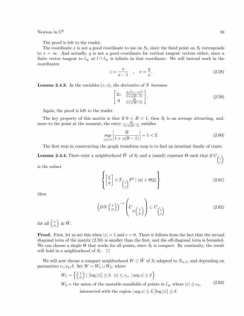
Newton in C2 39

The proof is left to the reader.The coordinate x is not a good coordinate to use on Sl, since the fixed point on Sl corresponds

to x = ∞. And actually, y is not a good coordinate for vertical tangent vectors either, since afinite vector tangent to l∞ at l ∩ l∞ is infinite in that coordinate. We will instead work in thecoordinates

z =x

x − 1, v =

y

x. (2.58)

Lemma 2.4.3. In the variables (z, v), the derivative of N becomes[

2z Az2(z−1)2

1+z(B−1)

0 B1+z(B−1)

]

. (2.59)

Again, the proof is left to the reader.

The key property of this matrix is that if 0 < B < 1, then Sl is on average attracting, and,more to the point at the moment, the entry B

1+z(B−1) satisfies

sup|z|=1

∣

∣

∣

∣

B

1 + z(B − 1)

∣

∣

∣

∣

= 1 < 2. (2.60)

The first step in constructing the graph transform map is to find an invariant family of cones.

Lemma 2.4.4. There exist a neighborhood W of Sl and a (small) constant Θ such that if C(

zv

)

is the subset

[

ξη

]

∈ T(

zv

)P2 | |η| > Θ|ξ|

(2.61)

then

(

DN(

zv

))−1

C

N

(

zv

)

⊂ C(

zv

) (2.62)

for all(

zv

)

in W .

Proof. First, let us see this when |z| = 1 and v = 0. There it follows from the fact that the seconddiagonal term of the matrix (2.59) is smaller than the first, and the off-diagonal term is bounded.We can choose a single Θ that works for all points, since Sl is compact. By continuity, the resultwill hold in a neighborhood of Sl. ¤

We will now choose a compact neighborhood W ⊂ W of Sl adapted to Nα,β , and depending onparameters ǫ1, ǫ2, δ. Set W = W1 ∪ W2, where

W1 =(

zv

)

∣

∣

∣

∣log |z|∣

∣ ≤ δ, |v| ≤ ǫ1, | arg z| ≥ δ

W2 = the union of the unstable manifolds of points in l∞ where |v| ≤ ǫ2,

intersected with the region | arg z| ≤ δ,∣

∣log |z|∣

∣ ≤ δ.

(2.63)


We will consider the variable z as “horizontal” and the variable v as “vertical,” and correspond-ingly we will set

∂HW1 = the part of the boundary where |v| = ǫ1

∂V W1 = the part of the boundary where |z| = e±δ

∂HW2 = unstable manifolds of points where |v| = ǫ2

∂V W2 = the part of the boundary where |z| = e±δ.

(2.64)

We will also consider the part of the boundary where arg z = δ as part of the horizontal boundary.Figure 20 shows these regions, with z drawn as 2-dimensional and v drawn as 1-dimensional; Figure21 is an attempt to draw their images (drawn separately for W1 on the left and W2 on the right.)

The invariant circle

The point at infinity

on the invariant circle

W1

W2

δ2ε1

ε2

−δ1e

δ1eε1

ε2

The disc of radius

ε2 in the line at ∞

The ‘‘top” and ‘‘bottom” surfaces

of W2 are made up of unstable

manifolds of points at infinity

Figure 20. A sketch of the regions W1 and W2. Of course, these are really 4-dimensional; we have

represented the coordinate v as 1-dimensional, whereas z is represented as a thickened circle in a plane,

which it indeed really is.

Figure 21. The images of W1 and W2, with the image of W1 on the left and W2 on the right. The space

W1 really maps “hyperbolically,” contracting in the vertical direction and expanding in the horizontal

direction. But W2 does not: the map does expand in the horizontal direction, but the horizontal boundary

is contained in the image of the horizontal boundary, since it is made up of unstable manifolds. With the

convention of the drawing, i.e., that v is 1-dimensional, one should imagine the top and bottom of W2 as

each a single unstable manifold, which is simply “spread out” over itself by z 7→ z2.

Newton in C2 41

We are now in a position to state our principal lemma, which allows us to set up a sort of “graphtransform.”

Lemma 2.4.5. We can choose ǫ1, ǫ2, δ so that if D ⊂ W is an analytic embedded disk with

TwD ⊂ Cw for every w ∈ D (D is almost vertical);

∂D ⊂ ∂H(W ) (D crosses W from top to bottom);

D ∩ |z| = 1, v = 0 is a single point (D crosses the circle);

then N−1(D) ∩ W has exactly two components that have the same properties.

Proof. Most of the difficulty in the proof is that we don’t have much control on where the unstablemanifolds of the points at infinity are: all we know is that the map Φ of Theorem 2.3.1 is analytic.Fortunately that is enough. It will be convenient to work with the parameter ζ = log z near z = 1.By the implicit function theorem, the unstable manifold through the point of coordinate w = y/xat infinity is the graph of a function σw, i.e., it has equation v = σw(ζ), at least for |w| sufficientlysmall.

Lemma 2.4.6. There exist ǫ0 > 0, δ0 > 0, and K such that

|σw(ζ) − w| ≤ K|ζ||w| (2.65)

when |ζ| < δ0, |w| < ǫ0.

Proof. Since the implicit function theorem applied to analytic data gives analytic implicit func-tions, the functions σw(ζ) are analytic functions that depend analytically on w, i.e., they are givenby convergent power series:

σw(ζ) = w + a1(w)ζ + a2(w)ζ2 + . . . . (2.66)

Moreover, ai(0) = 0 for all i, since σ0(ζ) = 0, reflecting the fact that l is the unstable manifold ofthe point at infinity on l. The result is now standard. ¤

Having found K, we can now choose δ1 > 0 sufficiently small that

B <1 − Kδ1

1 + Kδ1, (2.67)

and set δ = δ1/3, and ǫ1, ǫ2 satisfying

ǫ1 > ǫ2(1 + Kδ1), ǫ1 < ǫ2(1 − Kδ1), (2.68)

which is possible by Equation (2.67). We will require that ǫ1, ǫ2, δ1 have all been chosen sufficientlysmall that W ⊂ W , so that our invariant cone fields exist. From here on we will not change δagain, but we may need to further shrink ǫ1, ǫ2, making sure that they always satisfy Equation(2.68). The requirements we want are:

• for all (z, v) ∈ W1, the second coordinate of NF (z, v) is smaller than |v|;• the cone C(

z0

) intersects only the horizontal boundary of W .

We claim that with these requirements, Lemma 2.4.5 is true. This is mainly a matter of seeingthat the image of the interior of W does not intersect the horizontal boundary of W . This shouldbe clear if both the point (z, v) and its image (z1, v1) are in W1, since NF contracts strictly in thevertical direction in W1, so |v1| < |v|. It should also be true if the point and its image are in W2:the point is on some stable manifold, its image is on the same stable manifold, and this manifold


is not on the boundary of W2. The case where the point is in W2 and its image is in W1 is slightlymore complicated: it is on the manifold of a point w with |w| < ǫ2, and so is its image. Moreover,| log z| < δ1/2, so log z1| < δ1, and

|σw(z1)| < |w| + Kδ < ǫ2 + Kδ < ǫ1. (2.69)

The hardest case is if a point (z, v) ∈ W1 is mapped to a point (z1, v1) with | arg z1| < δ ande−δ < |z| < eδ; in this case, (z1, v1) ∈ W2, and is not on the horizontal boundary of W2. Thehypothesis implies that z1 is close to −1, and the normal multiplier in the entire left half-plane isat most |B|. So |v1| < |Bv|, and the unstable manifold through (z1, v1) will intersect the line atinfinity at a point v2 with |v2 − v1| < Kδ, hence with |v2| < Bǫ1 + Kδ < ǫ2.

The conditions we have set up will still be satisfied if we replace Nα,β by Nα′,β′ , with the point(α′, β′) chosen sufficiently close to (α, β); W1 is kept precisely as it was; and W2 is chosen as theunion of the unstable manifolds of the same points z = 1, |v| < ǫ2 for the new map.

Now suppose that z21 = z2, and that D crosses the circle at z2. There is then a unique component

D′ of N−1(D) ∩ W that contains z1, and D′ is an analytic disc in P2. Our first requirementguarantees that D intersects only the horizontal boundary of W , so the thing to check is that nopart of ∂D′ is in the interior of W . If a sequence in D′ converges to a point of the boundary ofD′ that is an interior point of W , its image also converges to an interior point of W , and this is acontradiction. ¤

The two lemmas together show that the graph transform map is well defined.Set X1 to be the polar locus, and Xn+1 = N−1

F (Xn). Let Yn,k be the component of Xn ∩ Wthat contains the dyadic root of unity ζn,k = e2πik/2n

. Moreover, let ǫ = ǫ2 − Kδ.

inCorollary 2.4.7. Each Yn,k is the graph Γfn,kfor some fn,k : Dǫ → C expressing z as a

function of v ∈ Dǫ, with fn,k(0) = ζn,k.

Proof. This follows immediately from Lemma 2.4.5. ¤

Let ∆ ⊂ Sl be the set of dyadic angles.

inCorollary 2.4.8. The map h : ∆ × Dǫ → C given by

h : (ζn,k, v) 7→ fn,k(v) (2.70)

is a holomorphic motion parametrized by Dǫ.

Proof. All the conditions for a holomorphic motion are clearly satisfied: the map is clearlyinjective and analytic with respect to v. ¤

We can now prove Theorem 2.4.1. By the λ-lemma ([MSS]), the map h extends to a maph : Sl ×Dǫ → C, quasiconformal with respect to z and analytic with respect to v. The set Vl is theimage of h, parametrized by Sl × Dǫ where u = h(ζ, v) is a 3-dimensional manifold, and N mapsVl to itself. Since the diagram

Vl −→ Vl

↓ ↓Sl −→ Sl

(2.71)

commutes on the set parametrized by ∆ × Dǫ, it commutes on Sl × Dǫ. Since the fibers of theprojection pr1 are graphs of analytic functions, they are analytic discs. ¤ Theorem 2.4.1

Newton in C2 43

In Figures 22–24 we give examples to demonstrate both why the boundaries of the basins looksmooth, and why they are not. If a bundle Vl as above exists, we should see it as a line separatingthe red and green basins.

Figure 22. This represents the line y = .1x, as parametrized by x, where we have −1 ≤ Re x, Im x ≤ 2,

for the Newton map where α = β = −1. The circle in the x-axis (which is the straight line Re x = 1/2) has

multiplier B/(B − 1) = 2/3, so it is attracting, and in fact has a stable manifold by Theorem 2.4.1. You

would expect this stable manifold to cut the line y = .1x along a quasi-circle close to the line Re x = 1/2.

Indeed, this is the case. Note the complicated decorations in the basin of the origin, red in the picture; one

bubble sequence is blown up at right. This is also as one would expect: the bubbles arise because there is

a point of indeterminacy on the x-axis, and they are in the red basin because the point of indeterminacy

is in the red basin. They present a dyadic structure, as they should.

Figure 23. This represents the line of equation y = .6x, for the same Newton’s method as above. This

time, we are plotting 1/x, i.e., near the point at infinity. The undulations of the quasi-circles are very

apparent.


Figure 24. This represents the line y = .1x, for the Newton’s method with α = −1, β = 3. This is

actually conjugate to the one above, but this time the circle in the x-axis is repelling (with multiplier 2,

since the point of indeterminacy is on it). When we perturb the slope away from 0, we would not expect

a curve to separate the red and green basins, and indeed there is no such curve; instead, a zone of blue

appears. On the right, we see the same line, but this time near infinity. Since the red and green basins

touch along the line at infinity, they must touch along its inverse images, which have a dyadic structure.

That is what one observes.

2.5. The extension of Φ and the origin of “bubbles.”

The mapping

ψm(w) = Φ−1(w, m) (2.72)

is a priori defined, analytic, and injective on some small disc Dr, and satisfies ψm(0) = [1 : m : 0]

and ψm(2w) = NF (ψm(w)) for w ∈ Dr/2. In other words, it is a linearizing parametrization of the

unstable manifold of [1 : m : 0]; moreover, it depends analytically on m ∈ C∗.

inProposition 2.5.1. For each m ∈ C∗, the mapping ψm extends to an analytic mapping ψm :C → P2.

Proof. The extension is defined by the formula ψm(2w) = NF (ψm(w)). The only difficulty one

can run into is when ψm(w) is a point of indeterminacy, and even then there is no real difficulty.

On any disc D ⊂ C, the map ψm : D → P2 lifts to a mapping ψm : D → P2I , and NF : P2

I → P2 is

well defined. ¤

As we will see, the extended ψm is no longer injective; in fact, we expect the image to be in

general very wild, perhaps dense in all of C2.

Newton in C2 45

Another unpleasant feature is that the extended ψm does not depend continuously on m, and

this gives rise to one of the characteristic features of drawings in complex slices: bubble sequences.

We will now explore this phenomenon.

There are some values of m for which ψm can be completely understood, and in fact an explicit

formula can be given, namely those that are the slopes of the invariant lines. Within these invariant

lines the point at infinity is a repelling fixed point, and it is well known that at a repelling fixed

point of a rational function, the linearizing map extends to an entire meromorphic function.

For the map z 7→ z2 and the fixed point 1, this extended linearizing map is w 7→ ew. In the

form (1.24), the x-axis is an invariant line, mapped to itself by NF by the formula

NF

(

x0

)

=(

x2/(2x − 1)0

)

. (2.73)

If we set z = x/(x − 1), this becomes z 7→ z2. For this slope we have

ψm(w) =ew

ew − 1. (2.74)

In the w-plane, we see the imaginary axis mapping as a universal cover to the invariant circle

Re x = 1/2, and separating the inverse images of the basins of 0 and 1 (the roots are “at ±∞”).

This picture is a bit misleading. Somewhere on the invariant line is the point of indeterminacy

1/B, probably in one of the basins but maybe on the invariant circle, and its inverse image under

ψ0 is a geometric sequence with increment 2πi. The inverse images of these points give a “dyadic

structure” on a neighborhood of the imaginary axis, on one side only, as shown in Figure 25.

0

0

Figure 25. The dyadic structure of inverse images of points of indeterminacy. If the point generating

the structure is real, the dyadic pattern of points is as on the left, but if it is not real the pattern will look

skewed, as on the right. The right-hand side of Figure 29 shows such a distorted dyadic pattern.

inProposition 2.5.2. If ψ0(w0) =(

1/B0

)

, then ψm(w) is discontinuous at the point m = 0, w =2w0.


Proof. There is no difficulty in showing that Φ−1 can be extended analytically to the region|Re w| < Re w0 + ǫ, |m| < ǫ for ǫ > 0 sufficiently small. If r < ǫ, and m 6= 0 satisfies |m| < ǫ, thenthe points ψm(w) form a disc that passes very near the point of indeterminacy q1. If we blow thispoint up, the lift of this disc will come very close to the entire exceptional divisor, and its imagewill come very close to the image of the exceptional divisor, which is a straight line (a line tangentto both parabolas in the normalization (1.34).) But the original invariant line does not come closeto the image of the exceptional divisor. ¤

Thus we see something like the Picard-Lefschetz formula appearing: there is a “vanishing cycle”on the unstable manifolds ψm, whose images, as m tends to 0, tend to the union of the invariant lineand the image of the exceptional divisor. In the disc Dr above, and at all its forward and inverseimages, i.e., at all the points 2n(w0 + 2kπi), n, k ∈ Z, we should see all of the dynamics of theexceptional divisor. But for m sufficiently small, we should see them only in a small neighborhoodof the dyadic grid; at every other point w, ψm(w) is analytic as a function of m for m sufficientlysmall. This is the source of the bubbles.

What should one see in a bubble? Mainly a third basin. The point of indeterminacy is theintersection of two invariant lines. The disc ψm(Dr) above will intersect the other invariant linesomewhere, and a neighborhood of that point will be in the basin of the root to which the point ofindeterminacy is attracted in the other invariant line. Usually, the bubble is primarily made up ofthat basin, but with complications around the edges, which can range from other bubble sequencesin the simplest cases to horribly complicated things in other cases.

Interestingly enough, it appears that there are values of the parameters such that the images ofthe ψm enter only three basins, not all four, for m sufficiently small. For instance, when α = β = 2,

we have been unable to find any points of the basin of(

22

)

in the unstable manifolds parametrized

by ψm for |m| < .1. This has consequences for the Russakovskii-Shiffman measure (discussed inSection 3.3): it is then not true that the entire line at infinity is in the support of the measure.

Figure 26 represents the unstable manifold ψm(w) for m = .05(1 + i), and α = β = 2.

Figure 26. Left: a sequence of blue bubbles (blue = basin of

(

01

)

) in the red basin (red = basin of(

00

)

). Right: a blow-up shows what the green dot off the left-most blue bubble really looks like.

Newton in C2 47

In this case, the mapping is real, and we can easily visualize the unstable manifold and thebubbles.

Figure 27. The real picture of Newton’s method when α = β = 2. A line y = mx with m small will be

mainly red and green, with blue interruptions in the red, near the point of indeterminacy and its inverse

images. The blow-up at right shows red and green stripes near the point of indeterminacy; these stripes

correspond to the green balls in the red basin in Figure 26, right. There does not appear to be any gray

in either the real or the complex picture.

The examples above are misleadingly simple. Figure 28 shows what happens when α = i, β =(1 + i)/2, in the line y = .02x. The decorations around the boundaries of the bubbles are nowmuch more complicated, and all four colors are present in the picture.

Figure 28. More complicated bubbles


This picture brings out several interesting features. One is the undulations of the quasi-circle

making the boundary between the red and the green basin. Another is the dissymmetry between

the part above the origin (which corresponds to the point at infinity) and the part beneath. The

discussion in Section 2.2 shows that such lack of symmetry is to be expected when B is not real,

and indeed here B = (1 + i)/2 is not real.

Attracting circles with repelling cycles

It is perfectly possible for an invariant circle to be attracting on average, but to contain repelling

cycles. In that case, Pesin theory guarantees that the circle has a stable manifold almost every-

where; but of course the repelling cycle cannot have a stable manifold, and neither can its inverse

images, which are dense in the circle. No neighborhood of the invariant circle like the set W above

can exist, and neither can there be a “center-stable” manifold as above with sections that are

quasi-circles. It isn’t quite clear what to expect instead.

Our best guess is something like “Arnold tongues,” open tongues emanating from the repelling

cycle, and making islands in which one should see all sorts of forward behavior, leaving a Cantor

set of large measure; this set is the “measure-theoretic stable manifold.”

Figure 29. On the left, we see what looks like a stable manifold, separating the green and red basins, with

bubbles in the green basin exhibiting the normal sort of dyadic behavior. The vertical line has equation

Re z = 1− cos 2π/7 ≈ .3765, and should intersect the “circle” near the points ζ3,1 (at the top) and ζ3,6 (at

the bottom), since angles are computed on the circle viewed as the boundary of the outside (the basin of

the origin). The cycle containing ζ3,1 is repelling, as we saw, and the cycle containing ζ3,6 is attracting,

with multiplier of absolute value ≈ .4103. On the right, we see a first blow-up at the top, with many more

bubble sequences, but the circle still looks smooth. This region is blown up further in Figure 30.

To construct an example, notice that the multiplier of the 3-cycle φ(ζ3,k) is

B

1 + ω(B − 1)

B

1 + ω2(B− 1)

B

1 + ω4(B− 1)=

B3

B + (B− 1)(ω + ω2 + ω4) + (B− 1)2(ω3 + ω5 + ω6),

Newton in C2 49

where ω = e2πi/7. For the value B = .8 + .4i, the invariant circle in the x-axis is attracting (withaverage multiplier |B| =

√.89), but the 3-cycle φ(ζ3,k) is repelling, with multiplier of absolute

value ≈ 2.556. We will look in the line of equation y = .05x, and in the local coordinate z = 1/x.Moreover, we will draw the region −1 ≤ Re z ≤ 3, | Im z| < 2. In the x-axis itself, the invariantcircle is the circle of radius 1 centered at 1, with the basin of the origin outside and the basin of(

10

)

inside. At that scale, in the line y = .05x we see the “circle” shown in the left-hand side of

Figure 29. However, the apparent circle does not really exist. If we perform three further blow-ups,we find the structure on the right of Figure 30. Similar complications are dense on the entire circle,but at very small scales at most places.

Figure 30. On the left, a further blow-up of the right-hand side of Figure 29 shows problems with the

proposed “circle,” presumably the appearance of a “tongue” emanating from the repelling cycle. A further

blow-up gives some details of what one should see within such a tongue.

3

The behavior at infinity when a = b =

In this chapter we will study Newton’s method as applied to the two equations

y = x2, x = y2. (3.1)

The associated Newton’s method is

N :(

xy

)

7→ 1

4xy − 1

(

2x2y + y2

2xy2 + x2

)

. (3.2)

The dynamics of this map N = N0,0 is probably not substantially simpler than any other Na,b,

but the formulas are simpler. In Chapter 6 we will show that all the same phenomena occur for

all Na,b .

The specific mapping N was studied by Russakovskii and Shiffman. In [RS], they study rational

mappings P : Pn ∼∼> Pn, whose topological degree is greater than the degree of P−1(W ), where

W is a generic hyperplane. This is the case for the mapping above, with topological degree 4 and

algebraic degree 3. They prove that in this case there is an invariant measure; but in the case of

the mapping N they could not decide whether this measure charges the points of indeterminacy

at infinity. As an example of the untangling allowed by Farey blow-ups, we answer this in Section

3, showing that the points of indeterminacy are not charged, and in fact giving a fairly detailed

description of the measure.

3.1. The primitive space

Consider in P2 the union of the axes and the line at infinity. We will blow up the double points

at infinity, then all the double points created, then all the double points created, etc., creating

compact algebraic surfaces X0 = P2, X1, X2, . . . , together with mappings πn : Xn → Xn−1. Call

D0 ⊂ P2 the line at infinity, and Dn = π−1n (Dn−1), n ≥ 1. For each n, Dn is a union of rational

curves, intersecting each other transversally, and will be called the divisor at infinity of Xn.

We call the projective limit XP = lim←

n

(Xn, πn) of these surfaces the primitive space, for the

following reason.

Consider finite sequences Pi of elements of Z2 defined as follows:

P0 =(−1

0

)

,(

11

)

,(

0−1

)

,

P1 =(−1

0

)

,(

01

)

,(

11

)

,(

10

)

,(

0−1

)

,

P2 =(−1

0

)

,(−1

1

)

,(

01

)

,(

12

)

,(

11

)

,(

21

)

,(

10

)

,(

1−1

)

,(

0−1

)

,

. . . . . . . . . . . . . . . . . . . . . . . . . . .

(3.3)

and so forth, making Pn+1 by intercalating(

p1 + p2q1 + q2

)

between each pair of consecutive entries(

p1q1

)

and(

p2q2

)

of Pn. The Pn are made up of points whose coordinates are coprime. Two vectors

50

Newton in C2 51

(

p1q1

)

,(

p2q2

)

∈ Z2 are consecutive in some Pn exactly if |p1q2 − p2q1| = 1; we will call such vectors

neighbors.Set P = ∪nPn; this set is a lot like the set of rationals: the ratios p/q enumerate all the

rational numbers, except that each negative rational slope corresponds to two points, and one

point corresponds to ∞ (namely,(

01

)

). The order in which the vectors appear is like the Farey

sequence as a way of enumerating the rationals.

inProposition 3.1.1. The irreducible components of Dn correspond to the elements of the se-

quence Pn, in the sense that if(

pq

)

∈ Pn, then the curve in C2 parametrized by

t 7→(

tp

tq)

(3.4)

tends, as t → ∞, to a point of Dn that is an ordinary point of an irreducible component L(

pq

),

and every irreducible component is reached in this way.

We will prove the stronger result (Proposition 3.1.2) below, providing curves that tend to all thepoints of Dn, allowing us to parametrize these components. The underlying reason our constructionworks is that the function xqy−p extends to L(

pq

); this extension provides an isomorphism L(

pq

) →

P1. We will use this as follows: since p and q are coprime, there exist integers k and l such thatlq − kp = 1.

inProposition 3.1.2. The curve xqy−p = m is parametrized by

t 7→(

mltp

mktq)

, (3.5)

and the mapping

m 7→ limt→∞

(

mltp

mktq)

(3.6)

exists for m ∈ C∗ and is an isomorphism C∗ → L∗(

pq

), where L∗(

pq

) is the complement of the

two double points on L(

pq

). The limit point will be referred to as the point of coordinate m on

L(

pq

).

Proof. We will prove this by induction. Thus, we will assume that the statement is true for Xn,

and show it for Xn+1. Let(

p1q1

)

,(

p2q2

)

be two neighbors in Pn ordered so that p1q2 − p2q1 = −1.

Then the relations

m1 = xq1y−p1 , m2 = xq2y−p2 (3.7)

express x and y in terms of m1 and m2:

x = mp2

1 m−p1

2 , y = mq2

1 m−q1

2 . (3.8)


This shows that we can use (m1, m2) as coordinates. The blow-up is being performed at the pointm1 = ∞, m2 = 0, so coordinates on the blow-up are provided by

m3 = m1m2 and m2. (3.9)

In terms of x and y, we have m3 = xq1+q2y−(p1+p2), and the curve

t 7→(

tp1+p2

tq1+q2

)

is the curve m3 = 1, m2 = 1/t, (3.10)

So it does indeed lead to a point of L(

p1+p2

q1+q2

). ¤

3.2. Newton’s method and the primitive space

The reason this primitive space is of interest to us is that it almost represents a natural compact-ification of C2 to which Newton’s method almost extends.

Part of the reason for this is that the mapping N takes the x-axis to the y-axis, which is mappedback to the x-axis, by the formula

(

t0

)

7→(

0−t2

)

7→(

t4

0

)

. (3.11)

In Chapter 6, we will see how the primitive space must be modified when a and b are arbitrary; inthat case the axes have no particular dynamical significance, and we will need to use other curvesin their place.

inProposition 3.2.1. The Newton mapping extends as a rational map to the primitive space,giving NP : XP ∼∼> XP , with four points of indeterminacy:

• the point of coordinate −2 in L(

21

) and the point of coordinate −1/2 in L(

21

);

• the point of coordinate 4 in L(

1−1

) and the point of coordinate 1/4 in L(

−11

).

Note that the points of the first pair are at the intersections of D∞ with the parabolas x+2y2 = 0and y + 2x2 = 0; each of these parabolas is one component of the inverse image of the x-axis andthe y-axis (the axes are tangent to a critical value parabola at a root, so the inverse images arein agreement with Proposition 1.5.1). The points of the second pair are at the intersection of D∞with the polar hyperbola of equation 4xy = 1.

Proof. The curve parametrized by

t 7→(

mltp

mktq)

, (3.12)

maps to the curve

t 7→ 1

4ml+ktp+q − 1

(

2m2l+kt2p+q + m2kt2q

2ml+2ktp+2q + m2lt2p

)

. (3.13)

We need to show that as t → ∞, this curve has a well defined limit in XP . This is a matter ofmaking sure what terms in the expressions above are dominant. To keep track of the various terms,let us consider the (p, q)-plane (in which one should remember that only the points with coprime

Newton in C2 53

integer coordinates, and at least one coordinate positive, represent components of D∞), broken up

as shown in Figure 31 into five zones.

1

2

34

5

Figure 31. The marked points of the grid correspond to components of D∞; the five zones are distin-

guished by the shading.

In the different zones, different terms are dominant, and the four points on the boundaries of

zones correspond to the components of D∞ where there are competing terms.

The mapping in zone 1: p + q < 0 and p > 0

In zone 1, the dominant terms are

t 7→ 1

−1

(

2m2l+kt2p+q

m2lt2p

)

. (3.14)

This breaks up into two cases, depending on whether q is even or odd.

If q is even, say q = 2q1, then the image component is L(

p+q1

p

), and the coordinate in that

component is

xpy−(p+q1) = (−1)q12pm−1. (3.15)

Thus we see that the component L(

pq

) is mapped by an isomorphism to the component L(

p+q1

p

).

However, the even power of t in both coordinates means that this component is a critical curve: a

small circle around such a component is mapped to a circle that wraps twice around the image com-

ponent, much closer than the original circle. This will be a key consideration when understanding

invariant measures.


If q is odd, the situation is quite different. Then the image component is L(

2p+q2p

), and the

coordinate within this component is

x2py−(2p+q) = −22pm−2. (3.16)

Thus we see that the domain component is mapped by a rational map of degree 2 to its image,

with ramification at m = 0 and m = ∞.

The case of(

pq

)

=(

1−1

)

(on the boundary of zones 1 and 2)

The line L(

1−1

) is parametrized by t 7→(

t/mt−1

)

. This curve maps to

1

4/m − 1

(

2t/m + t−2

2m−1t−2 + t2/m2

)

. (3.17)

Clearly the first term dominates in the first coordinate and the second term dominates in the

second coordinate, so L(

1−1

) maps to L(

12

), with the point of coordinate m mapping to the point

of coordinate

x2y−1 =1

4/m − 1

4

m4(m2) =

4

m(4 − m), (3.18)

which is a rational function of degree 2.

Let us look a bit more carefully at this rational function. The point of coordinate m = 4 in

L(

1−1

) is one of the two points where the polar curve of equation 4xy = 1 intersects D∞ (the

other is in L(

−11

)). Since the polar curve maps to the line at infinity, which is L(

11

) in the present

notation, and L(

12

) does not intersect L(

11

), this will create a problem, and this point m = 4 will

be a point of indeterminacy of the extended Newton map.

How about critical points? The rational function 4m(4−m) has two critical points, at ∞ and

at m = 1/2. The latter is one of the intersections of the critical cubic C2 with D∞, and maps

to the point where the critical value parabola of equation y = x2 intersects D∞ in L(

12

). The

other critical point is accounted for, like all the critical points at 0 and ∞, by the fact that many

components of D∞ are themselves critical.

The case of zone 2: p + q > 0 and 2q < p

In zone 2, the parametrized curve

t 7→(

mltp

mktq)

(3.19)

is mapped to the parametrized curve

t 7→ 1

4ml+ktp+q − 1

(

2m2l+kt2p+q + m2kt2q

2ml+2ktp+2q + m2lttp

)

. (3.20)

Newton in C2 55

In the denominator the term tp+q dominates over the constant −1, otherwise again the first term

dominates in the first coordinate function and the second dominates in the second coordinate

function, so altogether we find as principal terms(

mltp/2

ml−ktp−q/4

)

. (3.21)

Thus the image of L(

pq

) is the line L(

pp−q

), and the point with coordinate m is mapped to the

point of coordinate

xp−qy−p = 2p+qm(p−q)ltp(p−q)m−p(l−k)t−p2+pq = 2p+qm−1. (3.22)

We see that the line L(

pq

) is mapped to the line L(

pp−q

) by an isomorphism.

The case of the line L(

21

) (on the boundary of zones 2 and 3)

A computation just like the ones above shows that the parametrized curve

t 7→(

mt2

t

)

, (3.23)

leading to the point with coordinate m on L(

21

), maps to the curve with principal terms

t 7→ 1

4mt3

(

2m2t5

2mt4 + m2t4

)

=

(

mt2/2

(2 + m)t/4

)

, (3.24)

with the two terms in the second coordinate in competition. Thus this line maps to itself, with

the point of coordinate m mapping to the point of coordinate

xy−2 =mt2

2

(

4

(2 + m)t

)−2

=8m

(2 + m)2. (3.25)

This rational fraction plays an important role in the dynamics of Newton’s method at infinity.

It is dynamically quite simple, similar to the Chebychev polynomial z2 − 2. The Julia set is a

line segment, but instead of the complement being attracted to a superattractive fixed point, it is

attracted to a linearly attracting fixed point.

More specifically, the critical points are at m = ±2. The one at −2 maps to infinity, which maps

to 0, which is a repelling fixed point. The one at m = 2 is attracted to the attracting fixed point

at 2(√

2 − 1). The Julia set is the negative real axis, and its complement is entirely attracted to

the attracting fixed point.

This is the dynamics of the rational map, but doesn’t quite jibe with the 2-dimensional dynamics

of N . More specifically, the critical point m = 2 is on the critical cubic C1, and it maps to the

point m = 1 on the critical value parabola of equation x = y2. But the other critical point is much

more troublesome. It is on the parabola of equation x = −2y2, which maps to the x-axis, and

the point m = 0 on L(

21

) does not intersect the x-axis. As such, this point m = −2 is a point of

indeterminacy of the extended Newton map. We will need to blow it up again, and a lot of the

complications of the Newton map are hidden in this point.


The case of zone 3. In zone 3, the map is especially simple. There the first term dominates in

each coordinate, and the 4xy dominates in the coefficient, so the principal terms of the image of(

xy

)

are simply(

x/2y/2

)

. Thus every line in zone 3 is mapped to itself by the identity. But notice

the 2′s in the denominator; they indicate that in XP , all these lines are repelling. Of course, we

knew all about that in the case of L(

11

), from Section 2.3.

The cases of zones 4 and 5 and of the points(

12

)

and(−1

1

)

, are completely parallel to those

already covered, and we only give the results.


21

). This line is mapped to itself, by the rational function m 7→

(2m + 1)2/(8m), obtained from the case of L(

12

) by conjugating by m 7→ 1/m.

The case of zone 4. The line L(

pq

) is mapped to the line L(

q−pq

) by the isomorphism m 7→

2−(p+q)m.


−11

). This line is mapped to L(

21

), by the rational map of degree 2

m 7→ (4m − 1)/(4m2).

The case of zone 5. Again there are two cases. If p is even, say p = 2p1, then the image

of L(

pq

) is L(

pq+p1

), and the mapping is given by m 7→ (−1)q12−pm−1. Again in this case the

(

pq

)

-component is critical. If p is odd, the image of L(

pq

) is L(

2p2q+p

), and the mapping within

this component is m 7→ −2−2pm−2.

3.3. The asymptotic behavior of the Russakovskii-Shiffman measure

Although after all these blow-ups our Newton map still has points of indeterminacy, we have

blown up enough to untangle much of the dynamics at infinity. Russakovskii and Shiffman [RS]

have constructed a measure µ on P2 which describes the distribution of inverse images of points in

the finite plane C2. More specifically, they prove that if f : P2 ∼∼> P2 is a rational mapping, whose

topological degree d is larger than the algebraic degree, then there is a pluripolar exceptional set

E ⊂ P2 such that if x ∈ P2 − E, then the sequence of probability measures

µn =1

dn

∑

y∈f−1(x)

δy (3.26)

converges to a limit independent of x.

The mapping considered here is one of their examples, but they could not determine whether

this measure charges the points of indeterminacy p1 and p2, though their computer experiments

suggest that it does not. We will prove that this is indeed the case.

The difficulty is that near these points, Newton’s method displays several different kinds of

behavior, both attracting and repelling. The blow-ups we have performed in Sections 3.1 and 3.2

Newton in C2 57

will allow us to tease these various behaviors apart. Guided by the blow-ups, we will chop up aneighborhood of infinity in C2 as follows. Let UK be the locus where sup|x|, |y| ≥ K.

The two lines L(

32

) and L(

23

) are both in zone 3, hence fixed, and normally repelling with

multiplier 2. As such, every point has an unstable manifold, by Proposition 2.3.4. The adherenceof the 3-dimensional locus of equation |x|2 = |y|3 in C2 is a circle in L(

32

), which can also be

described as the locus |m| = 1, where m is the parameter on L(

32

) defined in Proposition 3.1.2.

There is a similar circle in L(

23

).

We will consider the unstable manifolds of these circles, i.e., the union of the unstable manifoldsof their points. These form two 3-dimensional manifolds, at least near infinity, and we can considerthe components M1, M−1 of these manifolds in UK containing the circles, which form bundles ofdiscs over the circles.

The components L(

32

) and L(

23

) have a sequence of inverse images, alternately near the point

at infinity on the x-axis and y-axis. Let us call the Mi the intersection of UK with N−1(M1−i), sothat the Mi march monotonically from the point at infinity on the x-axis to the point at infinityon the y-axis. These 3-manifolds cut up UK into regions Ak, k ∈ Z, as represented in Figure 32.

1

1

3

2

2

1

3

1

1

0

2

-1 1

-1

3

-4

1

-2

1

-4

2

31

2

1

30

1

-1

2-1

1

-4

3-2

1

-4

1

A0

A4

A3

A2

A1

A5

A-1A-2A-3A-4A-5A-6

1

-3

3

-14

1

-6

-3

1

-14

3-6

1

x

y

K

K

polarhyperbola

parabola

y=-2x2,inverse imageof x-axis

parabola

x=-2y2,inverse imageof y-axis

M-1

M1

M2

M3

M4

M5

M6

M-2M-3M-4M-4M-6

Figure 32. A schematic drawing of the sets Ak.


Clearly, we can choose K large enough that any finite number of these inverse images are

well-behaved, but knowing that all the inverse images are well-behaved requires proof.

Lemma 3.3.1. For K sufficiently large, each Mi cuts UK into two pieces, one containing all the

Mj , j < i, and the other containing all Mj , j > i.

Proof. Choose K large enough that the statement is true for i = −2,−1, 1, 2. For all the others,

near the component of D0 adherent to Mi, the Newton mapping is either of the form(

xy

)

7→( ∗−x2

)

or(

xy

)

7→(−y2

∗)

. (3.27)

Thus in this region, UK maps well inside itself, and is locally separated by M1−i. It follows that

the inverse image Mi separates UK . ¤

The manifolds Mi now allow us to build a “Markov partition” of UK ; we label Ak the closures

of the components of the complement of the Mi, ordered so that

Ai is bounded by Mi and Mi+1 when i > 0,

Ai is bounded by Mi and Mi−1 when i < 0,

A0 is bounded by M1 and M−1.

Moreover, we define Ak(C) ⊂ Ak to be the subset where ‖(

xy

)

‖ ≤ C; in particular, if C < K,

then Ak(C) = Ak(K) = Ak.

inTheorem 3.3.2. There exist numbers λk > 0, k ∈ Z, such that∑

k∈Z λk < ∞, and a cutoffK > 0, such that if we set

µk =

λk|dt|t2 if k is even

λk|dt|t3/2 if k is odd,

(3.28)

then whenever a probability measure ν on C2 satisfies

ν(Ak(C)) ≤∫ ∞

C

µk(t) dt (3.29)

for any C > K, the probability measure 14N∗ν also satisfies this inequality.

inCorollary 3.3.3. The Russakovskii-Shiffman measure σ does not charge the points p1 and p2.

Proof of Corollary 3.3.3. The measure σ is obtained by giving weight 1 to a generic point (off

an exceptional pluripolar set), then giving weight 1/4 to its inverse images, then weight 1/42 to

its inverse images, etc. This defines a sequence of measures σ0, σ1, . . . ; Shiffman and Russakovskii

prove that the sequence converges.

Clearly we can choose σ0 so that it satisfies Equation (3.29), for instance by choosing the initial

point outside of UK . Then all σn also satisfy (3.29), and so does σ. But for any ǫ > 0, there exists

K ′ such that any measure satisfying (3.29) assigns measure < ǫ to the region UK′ . ¤

Proof of Theorem 3.3.2. The proof will take six pages, so before giving it we will outline

what is really happening. The main content of the theorem is that on average, the initial points of

indeterminacy p1 and p2 are attracting. The problem is that this isn’t quite true: there are many

Newton in C2 59

inverse images near L(

12

) and L(

21

), and these are repelling. But they are only repelling linearly,

whereas elsewhere, more particularly near L(

1−1

) and L(

−11

), the map is superattracting, at least

with an exponent 3/2. We chose our domains Ak carefully so that this would be the case; the point

of having a domain like A2 at all was to keep A3 away from L(

10

), which is again repelling. Then

it is not surprising that the superattracting behavior wins out over the linearly repelling behavior;

this fact is quite specifically illustrated by the K1/4 in formula (3.38), which is really the key to

why the proof works at all.

We need to choose the numbers λk so that the pull-back of the measure µ itself is at most four

times itself. This is fairly easy for |k| ≥ 3, and for all k even, but choosing λ−3, λ−1, λ1, λ3 is

quite difficult: because of the points of indeterminacy, there are a lot of inverse images near these

points.

We will find inequalities which express that the theorem is true in each Ak; this is a different

problem in each Ak. We will start with the hardest case, A1. Let ν be a probability measure on

C2 such that ν(Ak(C)) ≤∫ ∞

Cµk(t) dt for all k ∈ Z.

Lemma 3.3.4. For any ǫ > 0, there exists K such that when C ≥ K, the measure N∗ν will satisfy

1

4N∗ν(A1(C)) ≤

∫ ∞

C

µ1(t) dt (3.30)

if

(2√

1 − ǫ −√

2)λ1 >√

2∞∑

k=1

λ2k+1 +1

√

K(1 − ǫ)

∞∑

k=1

λ2k +

√

2K(1 − ǫ2)

2. (3.31)

Proof. The region A1 maps two-to-one to the union of all the Ak, k > 1, and in this region the

x-coordinate of N(

xy

)

is x/2 +o(|x|). In particular, if we choose K sufficiently large, we will have

∣

∣

∣

∣

(

N(

xy

))

1

∣

∣

∣

∣

≥ |x|(1 − ǫ)

2, (3.32)

where the index 1 on the left-hand side means the first coordinate. Since N(A1(K)) is strictly

larger than ∪k>0Ak(K), we must allow for the possibility that the pull-back measure may pick up

mass from outside UK ; this mass is at most 1/2, since ν is a probability measure, and a point has

at most two of its inverse images in A1. We will represent this mass, rather wastefully, as a1/√

C,

where a1 must be chosen sufficiently large that

a1√

2(K + ǫ)≥ 1

2, i.e., a1 =

√

2K(1 + ǫ)

2. (3.33)


Thus we find

1

4(N∗ν)(A1(C)) ≤ 1

2

∞∑

k=1

ν

(

Ak

(

C(1 − ǫ)

2

))

+a1√C

≤ 1

2

( ∞∑

k=0

λ2k+1

∫ ∞

C(1−ǫ)/2

dt

t3/2+

∞∑

k=1

λ2k

∫ ∞

C(1−ǫ)/2

dt

t2

)

+a1√C

=

√

2

C(1 − ǫ)

∞∑

k=0

λ2k+1 +1

C(1 − ǫ)

∞∑

k=1

λ2k +a1√C

≤√

2

C(1 − ǫ)

∞∑

k=0

λ2k+1 +1

(1 − ǫ)√

CK

∞∑

k=1

λ2k +a1√C

(3.34)

which will indeed be smaller than

λ1

∫ ∞

C

dt

t3/2=

2λ1√C

(3.35)

if

(2√

1 − ǫ −√

2)λ1 >√

2∞∑

k=1

λ2k+1 +1

√

K(1 − ǫ)

∞∑

k=1

λ2k + a1

√1 − ǫ. ¤ (3.36)

Now let us deal with with A3, which maps to A−1 and to a part of A0; which part depends on

K.

Lemma 3.3.5. For any ǫ > 0, there exists K such that the measure N∗ν will satisfy

1

4(N∗ν)(A3(C)) ≤ µ3

(

A3(C))

(3.37)

for C ≥ K if

λ0

K5/2(1 − ǫ)3+

λ−1

K1/4(1 − ǫ)3/4≤ λ3. (3.38)

Proof. The region A3 maps into A−1 ∪ A0; moreover, in the part of A3 that maps into A1, the

second coordinate of the image is |x|3/2 + o(|x|3/2); see Figure 33. Thus for K sufficiently large we

have∣

∣

∣

∣

(

N(

xy

))

2

∣

∣

∣

∣

> |x|3/2(1 − ǫ) when |x| ≥ K. (3.39)

(The index 2 on the left-hand side indicates the second coordinate.) This map is 2 to 1 to its

image.

In the part of A3 that maps to A0, which is a neighborhood of the polar hyperbola, the situation

is better yet. For one thing, this part of A3 maps to the part of A0 where |y| > |x|; moreover, the

second coordinate is |x|3/8 + o(|x|3), so when K is sufficiently large we have∣

∣

∣

∣

(

N(

xy

))

2

∣

∣

∣

∣

>|x|3(1 − ǫ)

8when |x| ≥ K. (3.40)

This map is 1 to 1 to its image.

Newton in C2 61

2

-1

1

-1

3

-4

2

3

1

2

1

3

1

1

A-1

A3

A0

N(A3)

CK

C3/2

criticalcubic

Polarhyperbola

criticalvalueparabola

C2C3 N(A3)

p

p”

p’

q

q’

q”

Figure 33. A schematic drawing of the mapping N in A3. To understand its behavior in the real, we

must remember that one of the critical cubics passes through A3, and that the image of A3 is bounded in

part by the critical value parabola y = x2. The part of the neighborhood of the polar hyperbola where

|x| > C, shown in dark, maps into A0, also shown in dark. The points p, q and their inverse images

p′, p′′, q′, q′′ are drawn to help understand how the mapping can be 2-to-1 outside the neighborhood of the

polar hyperbola, and 1-to-1 inside it.

We can now argue as above:

1

4(N∗ν)(A3(C)) =

1

2ν(

N(

A3(C))

∩ A−1

)

+1

4ν(

N(

A3(C))

∩ A0

)

≤ 1

2ν(

A−1

(

C3/2(1 − ǫ)3/2)

)

+1

4ν

(

N

(

A0

(C3

8

)

))

≤ λ−1

2

∫ ∞

(C(1−ǫ))3/2

dt

t3/2+

λ0

4

∫ ∞

(C(1−ǫ))3

8

dt

t2

≤ 2λ−1(

C(1 − ǫ))3/4

+λ0

4

8(

C(1 − ǫ))3

≤ 2λ−1

K1/4C1/2(1 − ǫ)3/4+

2λ0

K5/2C1/2(1 − ǫ)3

(3.41)

which will indeed be smaller than

λ3

∫ ∞

C

dt

t3/2=

2λ3

C1/2if

λ0

K5/2(1 − ǫ)3+

λ−1

K1/4(1 − ǫ)3/4≤ λ3. ¤ (3.42)

Of course, exactly the same results hold for λ−1 and λ−3.


Now let us deal with λ0, λ±2, which is much easier.

Lemma 3.3.6. (a) For K sufficiently large, the inequality

1

4(N∗ν)

(

A0(C))

≤ µ0

(

A0(C))

(3.43)

is satisfied when C ≥ K if

λ0 >K(1 − ǫ)2

1 + 2ǫ(3.44)

.

(b) For any ǫ > 0, there exists K such that the inequality

1

4N∗ν

(

A2(C))

≤ µ2

(

A2(C))

(3.45)

is satisfied for C ≥ K if

λ2 >λ0

1 − ǫ+ K(1 + ǫ). (3.46)

Proof. For part (a), observe that A0 maps 1 to 1 to A0, and that when K is sufficiently large,we have

1

2

∥

∥

∥

(

xy

)∥

∥

∥(1 + ǫ) ≥

∥

∥

∥N

(

xy

)∥

∥

∥≥ 1

2

∥

∥

∥

(

xy

)∥

∥

∥(1 − ǫ) when

∥

∥

∥

(

xy

)∥

∥

∥≥ K. (3.47)

Again, we need to allow for the possibility that N∗ν picks up some mass from the mass of ν outsideUK . We will represent this mass as a0/C, where a0 = K(1 + ǫ)/2. Then for any C < 2K(1 + ǫ),i.e., for any C such that N(A0(C)) may fail to be contained in UK , the term a0/C is at least 1/4,which is the maximum mass N∗ν/4 can pick up, since ν is a probability measure.

Thus

1

4N∗ν

(

A0(C))

=1

4ν

(

A0

(C(1 − ǫ)

2

)

)

+a0

C≤ λ0

4

∫ ∞

C(1−ǫ)/2

dt

t2+

a0

C=

λ0

2C(1 − ǫ)+

a0

C, (3.48)

which is indeed smaller than

λ0

∫ ∞

C

dt

t2=

λ0

Cwhen λ0 >

2a0(1 − ǫ)

1 + 2ǫ. (3.49)

The second part is a bit more delicate, and requires cutting A2 in two so that the part A′2 with

|y| ≤ 1/2 + o(1) maps to the part of A0 with |y| > |x|, and the part A′′2 with |y| ≥ 1/2 + o(1) maps

to the part of A0 where |x| > |y|. In both cases, the map is 1-to-1, and in both the image spillsout beyond UK . We will represent the mass that N∗ν picks up from the mass of ν outside UK bya2/C, where a2 is chosen so that

a2

4K(1 + ǫ)≥ 1

4and

a2

2K(1 + ǫ)≥ 1

4i.e., a2 = K(1 + ǫ). (3.50)

In A′2, we have

∣

∣

∣

(

N(

xy

))

2

∣

∣

∣≥ |x|(1 − ǫ)

4. Thus we find

1

4N∗ν

(

A′2(C)

)

=1

4ν(

N(A′2(C))

)

≤ 1

4ν

(

A0

(C(1 − ǫ)

4

)

)

+a2

C

=λ0

4

∫ ∞

C(1−ǫ)/4

dt

t2+

a2

C=

λ0

C(1 − ǫ)+

a2

C.

(3.51)

Newton in C2 63

This is smaller than

λ2

∫ ∞

C

dt

t2=

λ2

Cwhen λ2 ≥ λ0

1 − ǫ+ a2. (3.52)

In A′′2 , we have

∣

∣

∣

(

N(

xy

))

2

∣

∣

∣ ≥ |x|(1 − ǫ)

2. Thus we find

1

4N∗ν(A′

2(C)) =1

4ν(

N(A′′2(C))

)

≤ 1

4ν

(

A0

(C(1 − ǫ)

2

)

)

+a2

C

=λ0

4

∫ ∞

C(1−ǫ)/2

dt

t2+

a2

C=

λ0

2C(1 − ǫ)+

a2

C.

(3.53)

This is smaller than

λ2

∫ ∞

C

dt

t2=

λ2

Cwhen λ2 ≥ λ0

2(1 − ǫ)+ a2, (3.54)

a fortiori when

λ2 ≥ λ0

(1 − ǫ)+ a2. ¤ (3.55)

Finally, we come to the conditions on the λk, |k| > 3. These present no difficulty: Ak maps

well inside A2−k, there is no spillover to worry about.

Lemma 3.3.7. For any ǫ, there exists K such that the inequality

1

4N∗ν

(

Ak(C))

≤∫ ∞

C

µk dt (3.56)

is satisfied for C ≥ K if

λk ≥ λ2−k√K(1−ǫ)

if k is odd

λk ≥ λ2−k

K(1−ǫ)2 if k is even.(3.57)

Proof. In all Ak with k > 3, the significant term of the Newton map is∣

∣

∣

(

N(

xy

))

2

∣

∣

∣= |x|2+o(|x|2);

more precisely, there exists K such that if |x| ≥ K, then∣

∣

∣

(

N(

xy

))

2

∣

∣

∣≥ (1 − ǫ)|x|2. (3.58)

Thus we find

1

4N∗ν

(

Ak(C))

=1

2ν(

N(Ak(C)))

≤ 1

2ν

(

A2−k

(

C2(1 − ǫ)2))

. (3.59)

We now study separately the cases k even and k odd.

If k is even, we have

ν(

A2−k

(

C2(1 − ǫ)2))

≤ λ2−k

∫ ∞

C2(1−ǫ)2

dt

t2

=λ2−k

C2(1 − ǫ)2≤ λ2−k

KC(1 − ǫ)2.

(3.60)


This will be smaller than

λk

∫ ∞

C

dt

t2=

λk

Cif λk ≥ λ2−k

K(1 − ǫ)2. (3.61)

If k is odd, we have

ν(

A2−k

(

C2(1 − ǫ)2))

≤ λ2−k

∫ ∞

C2(1−ǫ)2

dt

t3/2

=2λ2−k

C(1 − ǫ)≤ 2λ2−k√

CK(1 − ǫ).

(3.62)

This will be smaller than

λk

∫ ∞

C

dt

t3/2=

2λk√C

if λk ≥ λ2−k√K(1 − ǫ)

. ¤ (3.63)

We are now in a position to prove Theorem 3.3.2: to find K, ǫ and λk, k ∈ Z such that all theinequalities (3.31), (3.38), (3.44), (3.46), (3.57) are satisfied. Let us recopy them here:

(2√

1 − ǫ −√

2)λ1 >√

2∞∑

k=1

λ2k+1 +1

√

K(1 − ǫ)

∞∑

k=1

λ2k +

√

2K(1 − ǫ2)

2(3.31), again

λ3 ≥ λ0

K5/2(1 − ǫ)3+

λ−1

K1/4(1 − ǫ)3/4(3.38), again

λ0 >K(1 − ǫ)2

1 + 2ǫ(3.44), again

λ2 >λ0

1 − ǫ+ K(1 + ǫ) (3.46), again

λk ≥ λ2−k√

K(1−ǫ)if k is odd, |k| > 3

λ2−k

K(1−ǫ)2 if k is even, |k| > 3.(3.57), again

Let us consider first the associated homogeneous inequalities:

(2√

1 − ǫ −√

2)λ1 >√

2∞∑

k=1

λ2k+1 +1

√

K(1 − ǫ)

∞∑

k=1

λ2k (3.64)

λ3 ≥ λ0

K5/2(1 − ǫ)3+

λ−1

K1/4(1 − ǫ)3/4(3.65)

λ0 > 0 (3.66)

λ2 >λ0

1 − ǫ(3.67)

λk ≥ λ2−k√

K(1−ǫ)if k is odd, |k| > 3

λ2−k

K(1−ǫ)2 if k is even, |k| > 3.(3.68)

These can be satisfied as follows: first choose ǫ > 0 small (for instance 1/4), and K so large

that all the asymptotic inequalities for N are true for ‖(

xy

)

‖ > K. Choose λ0 = 1, then λ2 so

that the fourth inequality is true, then λ3 so that the strict inequality

λ3 >λ0

K5/2(1 − ǫ)3(3.69)

Newton in C2 65

is satisfied. Now choose λk, |k| > 3 so that the fifth inequalities are satisfied, and so that the seriesin the first inequality is convergent. Now choose λ1 so that the first inequality is true. Next, chooseK larger yet so that the K1/4 in the denominator in the second inequality allows it to be satisfiedtoo.

We now have numbers that satisfy the homogeneous inequalities. Multiply all the λ’s by asufficiently large constant so that all the inhomogeneous inequalities are satisfied also. ¤

4

The Farey blow-up

In this chapter, we will pin down exactly what operation was performed when we constructed

the primitive space. More specifically, we define a new way of “blowing up a surface” at a point

(actually, an enriched point), which we call the Farey blow-up. The Farey blow-up has some very

pleasant naturality properties, and is probably the only way of constructing a natural domain for

a rational map with both points of indeterminacy and critical curves. We will proceed to compute

the cohomology of the smooth part of the Farey blow-up, and describe the real oriented blow-up

of the Farey blow-up along its exceptional divisor.

4.1. Definition of the Farey blow-up

Let X be a complex surface. An enriched point of X will be a point x ∈ X and two germs of smooth

curves C1, C2 that intersect transversally at x. Denote such an enriched point by x = (x, C1, C2);

the information x, C1, C2 will be called Farey data.

We define the Farey blow-up F(X, x) of X at x with respect to C1, C2 to be the pro-algebraic

variety obtained as the projective limit of the surfaces Xn, with divisors En ⊂ Xn, where

X0 = X, E0 = C1 ∪ C2 (4.1)

and Xn+1 is Xn blown up at all the double points of En that project to x.

The mappings of the projective system are the canonical projections πn+1 : Xn+1 → Xn.

The Farey divisor F(x) ⊂ F(X, x), which is the projective limit of the En, is a union of infinitely

many irreducible components, all of which contain two non-algebraic points.

1

1

2

1

1

2

3

2

3

1

1

3

2

3

3

4

3

5

2

5

1

4

4

3

5

3

5

2

4

1

Figure 34. The Farey divisor is topologically a chain of beads: spheres that touch on a Cantor set.

Any two smooth curves that intersect at a point can be represented locally as x = 0, y = 0 in

appropriate local coordinates, so Example 4.1.1 is a model for all Farey blow-ups.

Example 4.1.1. Let us compute the Farey blow-up of C2 at the origin, with respect to the x and

the y axes; so let 0 be the Farey data consisting of the origin and the two axes.

66

Newton in C2 67

In this case, the appropriate Farey tree is the obvious one, shown in Figure 35:

(

01

) (

10

)

F0(

11

)

F1(

12

) (

21

)

F2(

13

) (

23

) (

32

) (

31

)

F3

. . . . . . . . . . . . . . . . . . . . . . . . . . .

Figure 35. To get the entry between two entries, the corresponding coordinates are added; for example,

the entry

(

12

)

on line F2 is gotten by adding the entry

(

01

)

on line F0 and

(

11

)

on line F1; the entry(

31

)

on line F3 is gotten by adding the “parents”

(

21

)

on line F2 and

(

10

)

on line F0.

Let us denote by Fn the vectors in the nth line (starting at F0). Evidently the irreduciblecomponents of Xn can be labeled by the elements of Fn, as shown in Figure 36.

0

1

1

0 1

1

0

1

1

0

1

11

22

1

1

3

2

3

1

2

1

1

3

22

13

1

0

10

1

1

01

0

Figure 36. The first four stages in constructing the Farey blow-up F(C2, 0). The components (actually

rational lines) are represented as line segments, labeled by the pairs of integers appearing in the first four

stages of the Farey tree.

Since p and q are coprime, the pair(

pq

)

is completely specified by the slope p/q of the ray

through it. To lighten the notation, and also to make a distinction with a slighly different con-struction in Chapter 5, we will label the components of the Farey blow-up Lp/q.


There is a much deeper relation between a component Lp/q of D∞ and the vector(

pq

)

that

labels it: as t → 0, the parametrized curve t 7→(

tp

tq)

tends to a point of the component labeled

by(

pq

)

. As in Section 3.1, this statement can be sharpened.

Since p and q are coprime, there exist integers k and l such that lq − kp = 1. Then the limit as

t → 0 of the parametrized curve

t 7→ (mltp, mktq) (4.2)

exists in F(C2, 0) and these limits are all distinct for m 6= 0. The number m parametrizes the(

pq

)

component of F(C2, 0).

This provides a fairly complete description of the smooth points of F(C2, 0), but there are other

points. We next give an embedding of the positive irrationals into the Farey blow-up. Given a

positive irrational α, it lies between two consecutive elements(

p1q1

)

and(

p2q2

)

of Fn, in the sense

that p1/q1 < α < p2/q2. Set xn(α) to be the point

xn(α) = E(

p1q1

) ∩ E(

p2q2

). (4.3)

Since πn(xn(α)) = xn−1(α), the sequence x0(α),x1(α),x2(α), . . . defines an element x(α) of the

Farey blow-up F(C2, 0). It should be clear that the map R+ − Q → F(C2, 0), α 7→ x(α) is

injective, since between any two distinct irrationals there are rationals.

Such points x(α) are extremely singular. For instance, every neighborhood of such a point x(α)

has infinite-dimensional homology.

Notice that in analogy to the curves t 7→(

tp

tq)

, the curve

t 7→(

ttα

)

(4.4)

tends to the point x(α) of F(C2, 0).

We have now described almost all the points of F(C2, 0); the only ones missing are the points

of the irreducible components corresponding to m = 0 and m = ∞. They are also at the end of

curves: for instance, the curves

t 7→ (tp, tq log t) and t 7→ (tp log t, tq) (4.5)

tend to such points.

There is quite a bit of freedom in the order in which the blow-ups involved in a Farey blow-up

are performed.

Let X be an analytic surface, and x = (x, C1, C2) be an enriched point. If you blow up first x,

then some of the double points created, then some of the double points created, etc., finitely many

times, you will end up with a divisor D with double points on a surface Y . The components of D

form a chain, each intersecting two others, with the first intersecting the proper transform of C1

and the last intersecting C2; the components can be labeled by pairs of integers as above.

Newton in C2 69

inProposition 4.1.2. (a) The pairs of integers appearing as successive labels on D are neighbors.

(b) The space obtained by performing Farey blow-ups at all the double points of D is preciselyF(X, x).

(c) Conversely, the part of a Farey blow-up appearing between components with neighboringlabels can be blown down, and the quotient point is a smooth point, where the images of thetwo components intersect transversally.

Proof. Part (a) follows from the fact that the Farey sum of two neighbors is a neighbor to both

its parents.

Part (b) is more or less obvious: any double point y = L1 ∩ L2 of D appears at some point in

the construction of F(X, x), since all neighbors are adjacent in some Fn, and the further blow-ups

that take place there to construct F(X, x) are precisely the ones involved in constructing F(Y, y),

where y is y enriched by L1 and L2.

Part (c) is exactly undoing part (b). ¤

Remark. You cannot blow down any segment of a Farey divisor between components whose labels

are not neighbors without creating singularities.

4.2. Naturality of the Farey blow-up

The ordinary blow-up has bad naturality properties with respect to maps with critical points: the

inverse images have to be taken in the sense of schemes, and this introduces complications which

the Farey blow-up was designed to avoid.

Example 4.2.1. Consider the mapping f :(

xy

)

7→(

x2

y

)

. If we blow up the origin both in the

domain and the range, then f does not lift to a map f : C(

00

) → C(

00

). On the contrary, the

exceptional divisor is collapsed to the point of the exceptional divisor corresponding to the critical

locus, except for one point of indeterminacy, which corresponds to the kernel of Df(

00

)

. We

must blow up again at that point in order to get a well-defined map, and after blowing up, the

new exceptional divisor is critical. A more natural thing is to blow up the subscheme defined by

the equations x2 = 0, y = 0. But that blow-up is a singular space, with a cone point; it is what

one obtains if one blows down the first exceptional divisor in the first construction, which has

self-intersection −2 after the second blow-up, and hence can be blown down, at the expense of

creating a singular point.

inTheorem 4.2.2. Let X, Y be complex surfaces, and f : X → Y be a finite analytic map; weare particularly thinking of maps with critical curves. Suppose that z is an enriched point ofY , such that f−1(z) is set-theoretically a union of enriched points of X. Then f extends to acontinuous mapping F(X, f−1(z)) → F(z); this mapping is analytic on the smooth points ofF(X, f−1(z)).

Proof. The statement is local on X, so we may assume that f−1(z) is a single point. The

hypothesis that f−1(z) is set-theoretically a union of enriched points of X is very strong, and we


will see that we may choose coordinates in the domain and in the range so that the Farey dataconsists of the coordinate axes in both the domain and range.

We will show that near f−1(z) the map can be written

f :(

xy

)

7→(

xk

yl

)

(4.6)

for positive integers k, l.Indeed, without loss of generality, we may assume that both z and f−1(z) are the origin, and

that both sets of Farey data are the axes. If f(

xy

)

=(

g(x, y)h(x, y)

)

, then g(x, y) = 0 defines the

y-axis, and h(x, y) defines the y-axis, i.e., there exist intergers k, l > 0 such that we can writeg(x, y) = xku1(x, y) and h(x, y) = ylu2(x, y) for some functions u1, u2 that do not vanish in aneighborhood of the origin. Let v1(x, y) and v2(x, y) be analytic functions such that vk

1 = xku1

and vl2 = ylu2. Clearly (v1, v2) form local coordinates in the range of f , and with respect to the

coordinates (x, y) in the domain and v1, v2 in the range, the map has the desired form (4.6).

In this form, it is easy to define f explicitly on the Farey blow-up: if t 7→(

atp

btq)

is a parametrized

path leading to a point of the Farey blow-up (on the component at rational slope l/k), then its image

is the parametrized curve t 7→(

aktpk

bqtlq)

, which tends to a point of the component corresponding

to the primitive point on the line of slope (q/p)(l/k). Set d = GCD(pk, lq); a careful look at the

formulas shows that the(

pq

)

component is critical if d > 1, mapping with normal degree d, and

is a covering of its image component of degree kl/d, ramified (if d < kl) at the two non-algebraicpoints. ¤

We will denote the mapping(

xy

)

7→(

xk

yl

)

by f(

kl

). It is the basic example of a map then can

be lifted to the Farey blow-up.

4.3. The real oriented blow-up of the Farey blow-up

The Farey blow-up is a priori a rather scary space. It contains an uncountable set of non-algebraicpoints, for which every neighborhood has infinite-dimensional homology, so it does not have thehomotopy type of a CW complex. We will now show that the topological structure of the Fareyblow-up is actually much simpler and understandable than one might fear, and actually in somesense very familiar.

Topologically, it is much easier to understand the Farey blow-up after “resolving its singular-ities,” using real oriented blow-ups as in [HPV]. The Farey blow-up has a real oriented blow-upthat is reminiscent of the structures encountered in the Kolmogorov-Arnold-Moser Theorem.

To keep the paper self-contained, we repeat the definition of the real oriented blow-up, which isa device to “open a variety along a subvariety,” i.e., to speak of “the complement of the interior ofa tubular neighborhood” without having to choose a tubular neighborhood.

The oriented blow-up XZ : step 1

Suppose X is a real algebraic manifold, and Z ⊂ X is an algebraic subset, perhaps with singulari-ties. Suppose U ⊂ X is a coordinate patch in which the ideal I(Z) of functions vanishing on Z isgenerated by m functions f1, . . . , fm : U → R; in other words, Z ∩U = f−1(0), where f : U → Rm.

Newton in C2 71

We need to say things in terms of ideals rather than in terms of equations defining the set because,for instance, the origin in R2 is defined by the equation x2 + y2 = 0, but the one function x2 + y2

generates a much smaller ideal than I(Z), which is generated by x and y.We can then define UZ ⊂ U × Sm−1 to be the closure of the set

(x, p) ∈ U × Sm−1 | f(x) 6= 0 and f(x)/|f(x)| = p

. (4.7)

By contrast, the blow-up is the closure of the set

(x, l) ∈ U × Pm−1 | f(x) 6= 0 and f(x) ∈ l

; (4.8)

the main difference is that we are now allowing for the orientability of the line l ∈ Pm−1.This actually defines the oriented blow-up only locally, but a standard result from algebraic

geometry [Har] says that the blow-up has a universal property, which allows us to glue the localblow-ups together uniquely. This result goes over to the oriented context, as is shown in [HPV1],allowing us to define a space XZ locally isomorphic to the model above.

The real oriented blow-up, step 2

Already we run into trouble when Z is the union of the axes in R2. The ideal I(Z) is generatedby the single function xy, so the space R2

Z ⊂ R2 × S0 is

(Q1 ∪ Q3) × 1 ∪ (Q2 ∪ Q4) × −1, (4.9)

where Qi denotes the closed ith quadrant.This isn’t quite what we want: the plane cut along Z, i.e., the disjoint union of the four closed

quadrants. We will replace the space XZ by a space B∗R(X, Z), which maps to XZ , and whose

points above x ∈ XZ are the ends of X − Z at x. This does not change the points with a basisof connected neighborhoods, but it does separate the first quadrant from the third and the secondfrom the fourth, as the points of contact of these quadrants each correspond to two ends.

More formally, let X be any topological space, and Y ⊂ X a closed subset. The endpointmodification E(X, Y ) is the space X, where every point y ∈ Y has been replaced by the set ofends of X − Y at y, i.e., by the points of the projective limit

lim←

π0(V − Y ), (4.10)

where π0 is the functor that associates to a space its set of connected components, and the projectivelimit is taken over all open neighborhoods V ⊂ X of y. The space E(X, Y ) comes with a naturaltopology, which we will leave to the reader to define (see [Dou], Vol. II, p.197–198), and there is acanonical map p : E(X, Y ) → X. We will denote by E(Y ) ⊂ E(X, Y ) the subset p−1(Y ).

inDefinition 4.3.1. Let X be a real algebraic manifold, and Z ⊂ X an algebraic subset. Thereal oriented blow-up B∗

R(X, Z) is the endpoint modification E(XZ , Z), with the exceptionaldivisor B∗

R(Z) ⊂ B∗R(X, Z) being E(Z) ⊂ E(XZ , Z).

The real oriented blow-up of a Farey blow-up

Let X be a complex surface containing two curves C1, C2 intersecting transversally at x ∈ X, anddefining an enrichment x of x. Let D be a divisor on X that may contain one, or both, or neitherof C1 and C2 (it may be empty). If it contains neither, we will assume that x /∈ D.


We want to understand the relation between the real oriented blow-up B+R (X, D) and the real

oriented blow-up B+R (F(X, x)),F(x) ∪ D).

To lighten notation, we will call this object B+F(X; x, D). It isn’t a priori clear what this is,

and we must take the projective limits in the proper order. Recall that F(X, x) is naturally the

pro-algebraic space

lim←

(Xn, πn). (4.11)

Each Xn contains a divisor En, which with our definition contains both C1 and C2. Let us define

Dn to be En ∪ D, from which C1, or C2, or both have been removed if they do not belong to D.

Here, removing a curve means taking the closure of the complement of the proper transform of

that curve.

The real oriented blow-ups B+R (Xn, Dn) form projective systems by Theorem 5.9 of [HPV]. We

then define

B+F(X; x, D) = lim←

B+R (X, Dn). (4.12)

To make a model for this object, we first define a way of taking the interval (0,∞), and “opening

all the rational numbers to intervals.” To be more precise, consider the functions η1, η2 : [0,∞) → Rgiven by

η1(t) =∑

0<p/q<t,(p,q)=1

e− sup(p,q) and η2(t) =∑

0<p/q≤t,(p,q)=1

e− sup(p,q). (4.13)

Then the map t 7→ It = [η1(t), η2(t)] associates to every rational number a closed interval, and to

every irrational number a single point. These intervals and points are all disjoint. The limit

limt→∞

η1(t) = limt→∞

η2(t) = a (4.14)

is finite, so we may think of η1 and η2 as being defined on [0,∞], and giving a homeomorphism of

“[0,∞] with the positive rationals opened” to J = [0, a].

We will put an appropriate “real oriented blow-up structure” on J × (R/Z)2, by defining a circle

action ∗ on the zones Ip/q × (R/Z)2. If t ∈ Ip/q, we will let the circle R/Z act on t × (R/Z)2 by

s ∗(

t, (α, β))

=(

t, (α + ps, β + qs))

. (4.15)

Because the integers (p, q) are coprime, this action is free, and the orbits of the action are

(p, q)-torus knots. If pn/qn converges to an irrational number ω, then the orbits of the circle action

converge to leaves of the irrational foliation of slope ω on the torus η1(ω) × (R/Z)2.

For the remainder of this section, we will assume that C1 and C2 are contained in D.

Let us consider the real oriented blow-up p : B+R (X, D) → X of X along D. This is a 4-

dimensional manifold with boundary; the part of the boundary above C1−x and above C2−xcarries a circle action, and the fiber above x is a torus T , which comes with an action of (R/Z)2,

so that the limit of the circle action on the part above C1 becomes the action of the first factor,

and the limit of the circle action on the part above C2 becomes the action of the second factor, as

shown on the left of Figure 37.

Choose a neighborhood U = U1 ∪ U2 of x in C1 ∪ C2; and identify p−1(U) with J × (R/Z)2, so

that on the part of boundary above ∂U1 the action of the first factor of (R/Z)2 coincides with the

circle action there, and so that on the part of boundary above ∂U2 the action of the second factor

of (R/Z)2 coincides with the circle action there.

Newton in C2 73

Figure 37. Left: a torus, with circle actions on the inside and the outside. Right: the torus now thickened

into a Cantor set of concentric tori, with zones between them corresponding to the rational numbers. One

should imagine these zones also filled with circle orbits, forming torus knots of all different kinds.

Now let us call Z the set B+R (X, C1∪C2), with the original circle actions on B+

R (C1∪C2)−p−1(U).

Within p−1(U), put the circle actions on the parts corresponding to rational numbers, as described

in Equation (4.15).

inTheorem 4.3.2. There is a homeomorphism

h : Z → B+F(X; x, D) (4.16)

that is the identity off a neighborhood of the modified T , and which preserves the circle andtorus actions.

Proof. Consider the intervals JN , where all the components of J −(

∪p/q/∈FNIp/q

)

have been

collapsed to points. There is a natural projective system

→ JN → JN−1 · · · → J0 = pt, (4.17)

and the projective limit is precisely the interval J .

There are corresponding quotients JN × (R/Z)2 → JN−1 × (R/Z)2, and using the identification

above, we can define spaces ZN , together with maps forming a projective system

· · · → ZN → ZN−1 → · · · → Z0 (4.18)

with projective limit Z.

So the theorem will follow from giving compatible homeomorphisms

. . . → ZN → ZN−1 → . . .↓ hN ↓ hN−1

. . . → B+R (XN , EN ) → B+

R (XN−1, EN−1) → . . .(4.19)

These will be constructed by induction. To start the induction, we choose a neighborhood U ′

of x in X, containing U . Then we can find a mapping

B+R (X0, E0) → B+

R (X0, E0) (4.20)

that collapses p−1(U1 ∪ U2) to the torus p−1(x) = (R/Z)2, which is otherwise injective, and the

identity outside of p−1(U ′). This defines a homeomorphism B+R (X0, E0) → Z0.

Now the construction of hN from hN−1 is precisely what is done in [HPV], Theorem 5.9. ¤

There is a straightforward modification of Proposition 4.3.2 in the case where D contains only

one of C1 or C2, or neither.

The cases where D contains either C1 or C2 are identical. If it contains C2, we start with

p : B+R (X, C2) → X; the fiber p−1(x) is now a circle, and the first thing is to thicken it to a solid


torus, and to identify this solid torus with D×R/Z, so that the R/Z-action on ∂D×R/Z coincideswith the given circle action. Use polar coordinates (ρ, θ) in D, with ρ ∈ J . Then in the regionsρ ∈ Ip/q we can define a circle action as above, and the resulting space is our candidate for a modelof B+F(X; x, C2). The main difference is that the fiber above the point where C1 intersects E∞is now a circle, not a torus.

If D contains neither C1 nor C2, the topological model consists of removing a small 4-ball aroundx, bounded by a 3-sphere. Then E1 is a rational curve, and B+

R (E1) ⊂ B+R (X1, E1) maps to E1 by

a map conjugate to the Hopf fibration. Represent E1 again in polar coordinates, where the radius,which now lives in [0,∞], should be thought of as belonging to J . Now repeat the constructionabove; the points where E∞ intersects C1 and C2 both have circles above them, linking in B+

R (E1).

4.4. Naturality and real oriented blow-ups

We saw in Section 4.2 that a map of the form(

xy

)

7→(

xk

yl

)

extends to the Farey blow-up F(C2, 0),

where 0 is the origin enriched by the two axes. Here we will see that the mapping also extends tothe real oriented blow-ups of the Farey blow-ups, and that the mapping there is much nicer thanone might expect: it is a covering map, and only ramified along one or two circles if we decide notto blow up the original enriching data.

inTheorem 4.4.1. (a) Let X, Y be complex surfaces, and f : X → Y be a finite analytic map.Suppose that z is an enriched point of Y , such that f−1(z) is set-theoretically a union of enrichedpoints of X. Let D be a divisor in Y , which contains z only if it contains C1 or C2 or both.Then f lifts to a continuous mapping

B+F(

X; f−1(z), f−1(D))

→ B+F(Y ; z, D). (4.21)

(b) This map is a covering map if D contains both C1 and C2. If C1 is not in D, then theproper transform of C1 is bounded by a circle in B+F(Y ; z, D); the inverse image of that circleis critical, mapping to its image with the same local degree as the degree of f on C1. Theanalogous statement holds for C2. These are the only places where the map fails to be a localhomeomorphism.

Proof. The statement is local in the domain, so we can specialize to the case of Example 4.1.1,i.e., to the case where f = f(

kl

).

There is no problem at the smooth points of the Farey divisor: if a component is critical ofnormal degree d, then circle orbits map to circle orbits with degree d. So let us consider a non-algebraic point, corresponding to “slope” r, in the range. If r is rational, it corresponds to eitherthe upper or the lower end of a component; let us suppose the upper end if that happens. At eachlevel of the Farey tree, the real number r is then bracketed between two rational numbers:

r′N =p′Nq′N

≤ r <p′′Nq′′N

= r′′N . (4.22)

The lower bracketing sequence will be eventually constant if r is rational.A basis of neighborhoods of the non-algebraic point is then provided by the sets

∣

∣

∣

∣

x

y

∣

∣

∣

∣

r′

N

<1

ǫ,

∣

∣

∣

∣

x

y

∣

∣

∣

∣

r′

N

> ǫ,

| arg x − λ1| < ǫ, | arg y − λ2| < ǫ, |x|2 + |y|2 < ǫ.

(4.23)

Newton in C2 75

The inverse image of such a neighborhood by the mapping(

xy

)

7→(

xk

yl

)

is evidently the union

of kl disjoint sets, each of which contains such a set for a smaller ǫ. So the mapping on the realoriented blow-up is continuous, of constant degree kl. ¤

4.5. Homology of the Farey blow-up

In this section we will see how the homology of the smooth part of a surface on which a Fareyblow-up has been performed at an enriched point is related to the homology of the original surface.

Remark. It isn’t clear what the homology of the Farey blow-up itself is (as opposed to itssmooth points). This space has the sort of complication present in the Hawaiian earring, so we canexpect singular and Cech homology to be different. In fact, it seems more reasonable to study thecohomology of F(X, z), but we will not consider this problem. Instead, we will develop a notionof completed homology, which is a Hilbert space and hence isomorphic to its dual, and which willserve as both homology and cohomology.

Let X is a complex surface, and z be an enriched point of X. We will denote by F∗(X, z) ⊂F(X, z) the subset of smooth points. The space F(X, z) is a projective limit of spaces Xn withdivisors En. Let us denote X∗

n the surface Xn from which the double points of En have beenremoved. There are then natural inclusions

X∗0 ⊂ X∗

1 ⊂ X∗2 ⊂ . . . , (4.24)

and the increasing union is F∗(X, z), which is thus represented as an inductive limit.A first thing to realize (see Propositions 4.5.1 and 4.5.2) is that the homology is naturally a

subgroup of

H2(X) ⊕ ZIrr E∞ = H2(X) ⊕ ZQ∗

+ , (4.25)

where the second factor is the product (not the sum) of copies of Z, i.e., it consists of givingarbitrary integer weights to the components of E∞, which are naturally labeled by the positiverationals Q∗

+. Of course, it isn’t the entire group, for instance because it is countable, and theproduct group is uncountable. But neither is it H2(X) ⊕ Z(Irr E∞), where all but finitely manycoefficients vanish.

For the next proposition, it is essential to realize that removing a point (or finitely many points)from a complex surface does not change its second homology group; in particular the inclusionX∗

n → Xn induces an isomorphism H2(X∗n) = H2(Xn). This has the consequence that the compo-

nents Lp/q for(

pq

)

∈ Fn represent homology elements [Lp/q] of H2(X∗n).

inProposition 4.5.1. For each n, the homomorphism

H2(X) ⊕ ZFn → H2(X∗n),

(

c, (αp/q)p/q∈Fn

)

7→ i∗c +∑

p/q∈Fn

αp/q[Lp/q] (4.26)

is an isomorphism.

Proof. This is the content of Proposition 4.6 of [HPV]. ¤

Thus any element of the homology is an element of the inductive limit

lim→

(H2(X∗n), i∗) = H2(X) ⊕ lim

→ZFn . (4.27)


Every element of this inductive limit is represented by a sequence vm ∈ ZFm , vm+1 ∈ ZFm+1 , . . .starting with some m.

inProposition 4.5.2. The weight assigned by vk to elements of Fl with l < k is independent ofk.

Proof. This follows from Proposition 4.8 of [HPV]. ¤

Proposition 4.5.2 provides an embedding of H2(F∗(X, z)) → H2(X) ⊕ ZIrr E∞ , but we willdescribe the image much more precisely. Let Q be the first quadrant in R2.

inDefinition 4.5.3. Let S be the commutative group of functions f : Q → R that

• are continuous;

• are piecewise-linear, linear except on finitely many rays through the origin with rationalslope;

• take on integer values on Q ∩ Z2; and

• vanish on the axes.

This group is a free commutative group on generators ep/q, p/q ∈ Q∗+, one for each positive

rational number, defined as follows. Each rational number first appears in the Farey tree as theFarey sum

p

q=

p1 + p2

q1 + q2(4.28)

of two numbers that appeared earlier (its parents). Let ep/q ∈ S be the function that is linear

except on the rays of slope through(

p1q1

)

,(

pq

)

, and(

p2q2

)

, and which assigns 1 to(

pq

)

and 0 to

(

p1q1

)

,(

p2q2

)

,(

01

)

,(

10

)

. (4.29)

Lemma 4.5.4. The elements ep/q, p/q ∈ Q∗+ are a basis of S.

Proof. Consider the subgroup Sn ⊂ S of functions that are linear except on rays passing throughelements of Fn. This is a space of dimension 2n − 1, and the 2n − 1 functions

ep/q,(

pq

)

∈ Fn − F0 (4.30)

belong to it. We need to know that they span, or equivalently, that they are linearly independent.Indeed, if a linear combination is 0, the the coefficients corresponding to each element of Fn−Fn−1

must vanish, since otherwise the linear combination would not be linear at that element of Fn −Fn−1. But then, for the same reason, the coefficient of each element of Fn−1 − Fn−2 must vanish,etc.

Thus the ep/q,(

pq

)

∈ Fn are linearly independent in Sn, so that every element of Sn can be

written∑

(

pq

)

∈Fn−F0

ap/qep/q, (4.31)

Newton in C2 77

with rational coefficients ap/q, and we need to show that these coefficients are all integers. Suppose

not, and let m ≤ n be the smallest index for which there exists(

pq

)

∈ Fm with ap/q not an integer.

This is a contradiction, since all the basis functions corresponding to indices m′ > m vanish at(

pq

)

, as do as the others of index m, and since all the earlier ones give integers at(

pq

)

, .

Clearly together the ep/q form a basis of lim→

Sn = S. ¤

There is an evident isomorphism Sn = ZFn , simply giving the values at the elements of Fn,and this isomorphism induces a canonical projection S → Sn given by restricting a function fto the points of Z2 that are in Fn. There is also a natural inclusion Sn → S, which consistsof extending linearly to each sector bounded by rays through points of Fn. This map inducesmappings in : Sn → Sn+1.

Let X be a complex surface, and z be an enriched point of X. We define a homomorphism

Φ : S → F∗(X, z) as follows. Choose p/q ∈ Q∗+, and suppose

(

pq

)

∈ Fn − Fn−1. There is then

an exceptional divisor Lp/q ⊂ Xn labeled(

pq

)

. Let φp/q : P1 → Lp/q be an isomorphism, and let

φ′p/q : P1 → X∗

n be a small deformation whose image avoids the double points.

Remark. You can only deform differentiably: analytically, exceptional divisors are rigid. Thedeformation can take place in an arbitrarily small neighborhood of Lp/q, but the deformed 2-spheremust intersect Lp/q since this curve has self-intersection −1.

Then φ′p/q : P1 → F∗(X, z) maps the fundamental class in H2(P1) to a well-defined element

Φ(ep/q) ∈ H2(F∗(X, z) (this is the definition of Φ). For Theorem 4.5.5, we need one more general-ity: the inclusion X − z → X induces an isomorphism H2(X − z) → H2(X); using its inversewe see that there is a canonical map H2(X) → H2(F∗(X, z)).

inTheorem 4.5.5. The mapping Φ and the canonical map H2(X) → H2(F∗(X, z)) induce anisomorphism

H2(X) ⊕ S → H2

(

F∗(X, z))

, (4.32)

which we will still call Φ.

Proof. The space F∗(X, z) is the inductive limit of the X∗n, and since homology commutes with

inductive limits, we see that what we need to prove is that for every n, the map

Sn ⊕ H2(X) → H2(X∗n) (4.33)

is an isomorphism, and that the diagrams

H2(X) ⊕ Sn → H2(X∗n)

↓ ↓H2(X) ⊕ Sn+1 → H2(X∗

n+1)(4.34)

all commute.This is proved by induction, starting with n = 0, where it is the isomorphism H2(X) = H2(X −

z), and going from step to step using Proposition 4.6 of [HPV]. ¤

Give S a quadratic form, by making distinct ep/q orthogonal, and setting e2p/q = −1. The spaces

H2(X) and F∗(X, z) both carry quadratic forms defined by intersection, and these are all relatedby the following statement.


inTheorem 4.5.6. If we take H2(X)⊕ S to be an orthogonal direct sum, then the isomorphism

Φ : H2(X) ⊕ S → H2

(

F∗(X, z))

. (4.35)

is an isomorphism of spaces with inner products.

Proof. Begin by representing all elements of H2(X) by cycles that avoid a neighborhood of z; thatis really the meaning of the isomorphism H2(X) = H2(X−z). Then our first exceptional divisorL1/1 is orthogonal to all of H2(X), and has self-intersection −1, being an exceptional divisor. Nowthe statement should be clear from the way Φ was defined. Every homology class, when it iscreated, is disjoint from all the previous ones, and has self-intersection −1. Of course, the samething is true of φ′

p/q(P1), thus none of these classes intersect any other class, and they all haveself-intersection −1. ¤

4.6. The action of mappings f(

21

) on homology

The next task is to see how the maps

f(

kl

) : F∗(C2, 0) → F∗(C2, 0) (4.36)

act on the homology. We will work this out only for the mapping f(

21

), which we will denote

simply by f for the rest of this chapter. This turns out quite nicely, but a general proof along thelines of the one given here would be very cumbersome.

Let us denote fQ : R2 → R2 the map

fQ :(

pq

)

=(

2pq

)

. (4.37)

inTheorem 4.6.1. The map induced by f on the homology is

f∗(

ep/q

)

= 2ep/q f−1Q . (4.38)

Proof. The idea is to work at a level of blow-up where ep/q has just appeared. Let the Farey

parents of(

pq

)

be(

p1q1

)

and(

p2q2

)

, and assume that q1 is even and q2 is odd. (The case q2 even,

q1 odd is identical, and q1 and q2 can’t both be even; we will deal with the case where both are odd

later.) Observe that(

p1q1/2

)

and(

2p2q2

)

are then neighbors, and we can consider the sequence of

two blow-ups in the domain and range represented in Figure 38.Note that the map f extends at the top and the bottom level, but not at the middle level, where

the divisor labeled

(

p1 + p2

q1 + q2

)

is collapsed to the point marked with a circle, except for one point

of indeterminacy, marked with a star.

The class ep/q is represented by the line Lp/q after one blow-up, and by Lp/q + L(p1+2p2)/(q1+q2)

after the second blow-up. This maps to

2L(2p1+2p2)/(q1+q2) + L(p1+2p2)/(q1/2+q2). (4.39)

Newton in C2 79

Domain Range

p1

q1 p2

q2

p1

q1/2

2p2

q2

p1

q1

p2

q2

p1+p2

q1+q2

p1

q1/22p2

q2

p1+2p2

q1/2+q2

p1

q1

p2

q2

p1+p2

q1+q2

p1

q1/2

2p2

q2

p1+2p2

q1/2+q2

p1+2p2

q1+2q2

p1+2p2

q1+2q2

Figure 38. The map f can be locally extended before doing any blow-ups (i.e., at the top level), and

after doing two blow-ups (i.e., at the bottom level), but it cannot be extended at the middle level (after

just one blow-up).

On the other hand, the class e(p1+2p2)/(q1/2+q2) is represented by L(p1+2p2)/(q1/2+q2) after oneblow-up in the range, and by

L(2p1+2p2)/(q1+q2) + L(p1+2p2)/(q1/2+q2) (4.40)

after two blow-ups.Thus the image of ep/q is represented by

e(p1+2p2)/(q1/2+q2) + L(2p1+2p2)/(q1+q2) = e(p1+2p2)/(q1/2+q2) + e(2p1+2p2)/(q1+q2), (4.41)

since L(2p1+2p2)/(q1+q2) is the last exceptional divisor.This is a formula for the action of f(

21

) on homology (at least in the unramified case), but it

isn’t quite clear that it is what the statement promised. Before dealing with that, let us find theanalogous formula if both q1 and q2 are odd.

This is covered by Figure 38 also: both parents of(

p1 + 2p2q1 + 2q2

)

have odd second coordinates;

we will leave it to the reader to see that all lines with such labels appear in this setting. HereL(p1+2p2)/(q1+2q2) is an exceptional divisor created by the most recent blow-up, so it represents(after two blow-ups) the class e(p1+2p2)/(q1+2q2), and it maps to

L(p1+2p2)/(q1/2+q2) = e(p1+2p2)/(q1/2+q2) − e(2p1+2p2)/(q1+q2). (4.42)

Now we need to understand these elements of the commutative group S as functions (see Def-inition 4.5.3). We will restrict our functions to the line q = 1 to draw them. The functions ep/q


restrict to tent functions, of course, but the miracle that makes things work is that if(

p′q′

)

is a

child of(

pq

)

, then ep/q ± ep′/q′ is also a tent function; the slopes are exactly what is needed for

this to happen. Thus Figure 39 explains why Theorem 4.6.1 is true.

2p1 q1

p1+2p2q1/2+q2

q1+q2

2p2 q2

2p1+2p2 q1+q2

p1+2p

2

q1/2+q

2

e2p

1+2p

2

q1+q

2

e

q1+q2p

1+2p

2

q1/2+q

2

e 2p1+2p

2

q1+q

2

e+

2

1

2p1 q1

p1+2p2q1/2+q2

2p2 q2

2p1+2p2 q1+q2

p1+2p

2

q1/2+q

2

e2p

1+2p

2

q1+q

2

e

q1/2+q2 p1+2p

2

q1/2+q

2

e 2p1+2p

2

q1+q

2

e+

1

Figure 39. Left: the sum e(p1+2p2)/(q1/2+q2) + e(2p1+2p2)/(q1+q2) is the tent function

2e(p1+p2)/(q1+q2) f−1Q .

Right: the difference e(p1+2p2)/(q1/2+q2) − e(2p1+2p2)/(q1+q2) is the tent function

2(e(p1+2p2)/(q1/2+q2)) f−1Q .

4.7. Homology spaces and Sobolev spaces

We defined the commutative group S in Definition 4.5.3. The vector space S ⊗Z C is evidentlya (negative definite) pre-Hilbert space, and it is very tempting to complete it with respect to itsinner product. This creates the completed homology space

H2

(

F∗(C2, 0))

= l2(Q∗+), (4.43)

i.e., the space of series∑

p/q∈Q∗

+

ap/qep/q with∑

|ap/q|2 < ∞. (4.44)

This is already a fairly familiar space, but quite surprisingly, it is also naturally an old friendfrom analysis, the Sobolev space H1

0(I) of continuous functions on g on [0, 1], whose distributionalderivative is in L2, and such that g(0) = g(1) = 0. We use a script H to avoid confusion withhomology; the subscript 0 indicates that the function vanishes at the endpoints.

Remark. In one dimension, the functions in H1 are automatically continuous, so it is reasonableto evaluate them at points.

In fact, our tent functions ep/q form a basis of H10(I) very similar to the basis provided by the

integrals of the Haar functions, where instead of the dyadic partition of the interval, we use theFarey partition.

Let I be the interval joining(

10

)

to(

01

)

in the (p, q)-plane. We will parametrize I by t 7→(

t1 − t

)

, and give it the measure |dt|, so it has length 1. The restriction to I maps S to a space

of functions on I. For future reference, we will specify what the image is.

Newton in C2 81

Lemma 4.7.1. The image of S is the space of continuous, piecewise-linear functions g : I → Rthat vanish at the endpoints, are linear except at finitely many points with rational coordinates,

and satisfy the integrality condition that for all positive rational numbers p/q, we have

(p + q)g(p/q) ∈ Z. (4.45)

Proof. This should be clear from Lemma 4.5.4: if you extend a function g as above to be

homogeneous of degree 1, you will find a continuous, piecewise linear function on the quadrant q,

and its value at(

pq

)

will be (p + q)g(p/q). ¤

inTheorem 4.7.2. The map f 7→ f |I induces an isometry of Hilbert spaces

Ψ : S → H10(I). (4.46)

Proof. Notice that the functions f |I are tent functions. First let us see that Ψ(ep/q) and Ψ(ep′/q′)

are orthogonal if p/q 6= p′/q′. By their definition, either the supports of Ψ(ep/q) and Ψ(ep′/q′) are

disjoint, or the support of one, say Ψ(ep/q), is contained in an interval where the other is linear,

hence its derivative is constant. Thus what we need to show is that∫

I

d

dtep/q

(

t1 − t

)

|dt| = 0. (4.47)

(The function ep/q

(

t1 − t

)

is represented in Figure 40.)

p1p1+q1

p2p2+q2

p1+p2p1+q1+p2+q2

1p1+q1+p2+q2

Figure 40. The function ep/q

(

t1 − t

)

.

This is clear from∫

I

d

dtep/q

(

t1 − t

)

|dt| = ep/q

(

10

)

− ep/q

(

01

)

= 0 − 0 = 0. (4.48)

Next, we need to show that∫

I

(

d

dtep/q

(

t1 − t

)

)2

|dt| = 1. (4.49)

Computing the integral of the square of the derivative of this function is elementary algebra,

which we leave to the reader. We must use q1p2 − p1q2 = 1, of course, to make the integral come

out to be 1.


This shows that Ψ is an isometric inclusion. Now we need to show that the image of S is dense,but that is fairly clear from Lemma 4.5.4: the derivatives of elements of S give all step-functionson I with rational discontinuities and integral 0. These are certainly dense in the hyperplane inL2(I) made up of functions with integral 0; for instance, they include the Haar basis. ¤

There is quite a bit of freedom in this description, corresponding to the freedom in Proposition4.1.2; we will need only the following special case.

inProposition 4.7.3. (a) If you draw the vertical ray Rc defined by p = c, q > 0 in Q, and giveit the measure |dq|/c, then the restriction of elements of S to Rc is an isometric inclusion ofS into H1(Rc), and the image of S ⊗Z C is dense in the subspace of H1(Rc) of functions that

vanish at the endpoint(

0c

)

of Rc.

(b) Consider the mapping g : Rc → Rc given by g(q) = q/2. Then

(fQ)∗f |Rc = g∗f |Rc. (4.50)

Proof. We need to show that the restrictions of the ep/q are an orthonormal family; this is acomputation just like the one to justify Equation (4.49), and we omit it. The density follows, forinstance, from the fact that S contains the Haar functions. ¤

5

The compactification when a = b =

In this chapter, we will construct a compact space X∞ on which the Newton map N of Chapter

3 is well defined. We will further analyze the topology of this space, showing that its behavior at

infinity is very reminiscent of the KAM theorem [Ar].

5.1. The tower of blow-ups when a = b =

We will now define a projective system of pro-algebraic spaces X0, X1, . . . . The spaces X0 and X1

have already been defined: they are respectively X0 = P2 and X1 = XP , the primitive space of

Chapter 3. These spaces come with finite subsets Zi ⊂ Xi, entirely made up of smooth points. We

will enrich the structure for some of these points; i.e., for some of the z ∈ Zi, we will define two

smooth germs of algebraic curves C1, C2 ⊂ Xi intersecting transversally at z. We may also need

to enhance some other points. This will mean adding enough extra information at those points to

define some finite sequence of blow-ups at these points.

This enhanced or enriched structure is denoted by Zi, and we will define Xi+1 = F(Xi, Zi),

where in this context F denotes making ordinary blow-ups at ordinary points, Farey blow-ups at

enriched points, and the appropriate finite sequence of blow-ups at the enhanced points.

Thus these spaces will naturally come with “blow-up maps” πi+1 : Xi+1 → Xi. We need to keep

track of the divisor at infinity Dn, defined inductively by setting D0 to be the line at infinity in P2,

and Dn+1 = π−1n+1(Dn). We will also need to keep track of the exceptional divisors corresponding

to the ordinary and enhanced points or enriched points; we will do this by setting E1 = q1,q2,q3and En+1 = π−1

n+1(En). (These points q1,q2,q3 are the points already seen in Equation (1.27);

they are unrelated to the q’s of Chapter 4.)

We will also construct maps Ni+1 : Xi+1 → Xi for i ≥ 1, which will extend in an appropriate

sense the Newton map N of Chapter 3.

Building X1 and X2 requires special constructions; after that everything has a unified definition.

Set X0 = P2, with Z0 consisting of the points p1 and p2. The set Z0 adds to this structure the

enrichment of p1 by the x-axis and the line at infinity, and the enrichment of p2 by the y-axis and

the line at infinity.

Now define X1 = F(X0, Z0); this is exactly our primitive space XP . The Newton map N

extends to a rational map NP : X1 ∼∼> X1 with four points of indeterminacy at infinity, one each

on the lines

L(

1−1

), L(

21

), L(

12

), L(

−11

). (5.1)

Here we are denoting components of D1 with vector indices, not fractions, because the primitive

points of QP are not quite specified by their slopes.

We will meet these points again, so we give them names: A1, B1, B2, A2.

• The polar hyperbola 4xy = 1 and the component L(

1−1

) will enrich A1, giving A1;

83


• The parabola x = −2y2 and the component L(

21

) will enrich B1, giving B1;

• The parabola y = −2x2 and the component L(

12

) will enrich B2, giving B2;

• The polar hyperbola 4xy = 1 and the component L(

−11

) will enrich A2, giving A2.

We set Z1 to be the union of these four enriched points and the three ordinary points q1,q2,q3,

and define X2 = F(X1, Z1). It is not quite so easy to define N2 : X2 → X1.

inProposition 5.1.1. The Newton map N extends to a mapping N2 : X2 → X1.

Proof. There is no difficulty on E2, the blow-ups of q1,q2,q3; this was done in Lemma 1.2.4.

The difficulty is to show that N extends to the Farey divisors corresponding to the enriched points

A1, A2, B1, B2. In all cases, this follows from Theorem 4.2.2, but one must make some preliminary

constructions to see how.

Begin by performing just three blow-ups on P2: one at p1, to create L(

10

); a second at the

intersection L(

10

) with the line at infinity (here called L(

11

)), to create the divisor L(

21

); and

finally, a third at the point of coordinate m = −2 on L(

21

), to create a line we will temporarily

call simply L. Call the surface constructed Y . We are now in a position to apply Theorem 4.2.2.

Indeed, the Newton map extends to a neighborhood of the union L(

10

) ∪ L(

21

) ∪ L, mapping

L(

21

) to itself by the rational function given by Equation (3.25). The line L is critical, mapping

to L(

10

), and finally L(

10

) maps to the line at infinity.

In particular,

• the point x1 where L meets L(

21

), enriched by L and L(

21

), maps to the point y1 of coordinate

0 on L(

10

), enriched by L(

10

) and L(

21

);

• the point x2 where L meets the proper transform parabola of equation x + 2y2 = 0, enriched

by L and the proper transform of the parabola, maps to the point y2 of coordinate ∞ on L(

10

),

enriched by L(

10

) and the x-axis.

Thus N extends to a mapping

F(Y, x1, x2) → F(Y, y1, y2). (5.2)

But in the domain, L together with the two Farey divisors is precisely the Farey divisor corre-

sponding to B1, whereas in the range, the Farey divisors corresponding to y1 and y2 are sub-Farey

divisors of the Farey divisor corresponding to p1, so the mapping is well defined with values in X1.

Newton in C2 85

Next, we need to extend the Newton mapping to the Farey divisor at A1; this is easier. Performin the domain P2 two blow-ups at p1, to construct first L(

10

) and then L(

1−1

). In the range

P2, perform two blow-ups at p2, to construct L(

01

) and L(

12

). Then the Newton map is a local

isomorphism from the enriched point A1 to L(

12

) ∩L(

11

), enriched by the lines themselves. Again,

Theorem 4.2.2 now provides the extension; note that the Farey divisor in the range is a sub-Fareydivisor of the divisor associated to p2, so the range is X1.

The constructions for B2 and A2 are completely parallel. ¤

Here is a more computational approach to the extension at B2.In the coordinates u = x

y and v = yx2 , the line L(

12

) becomes the axis u = 0, and the parabola

Py of equation y = −2x2 becomes the line v = −2. We know how to parametrize the componentsof the Farey blow-up in these coordinates: set u = mksp, v = mlsq, where kq−pl = 1. This meansto “parametrize” the components of the Farey blow-up by rational numbers p/q ∈ Q∗

+, so that ∞is on Py and 0 is on L(

12

) (see Figure 41).

1

11

21

3

0

1

-1

1

1

2

N

Py

y-axisp

q

0

1

1

0

Figure 41. This represents how the Farey blow-up of B2 maps to X1.

Then the point with these coordinates tends to the point of coordinate m of the(

pq

)

-component

of the Farey blow-up as s → 0. Set s = 1/t; changing back to the (x, y) coordinates, we see thatthe curve

x =tp+q

mk(−2tq + ml), y =

t2p+q

m2k(−2tq + ml)(5.3)

tends to the point of coordinate m of the(

pq

)

-component of the Farey blow-up.


Remark. These formulas represent x and y as Puiseux expansions in t with two terms. This is

typical: as we blow up more and more times, paths leading to the deeper blow-ups need to be

sneakier and sneakier, and require more and more terms. No finite Puiseux expansion gives paths

that lead to the points of the projective limit; these require series, and the curves leading to them

are necessarily transcendental. This sort of thing was explored earlier (for Henon mappings) in

[Bou], [BS].

The image of this curve is

m3k(−2tq + ml)2

4t3p+2q − m3k(−2tq + ml)2

( 2t4p+3q

m4k(−2tq+ml)3+ t4p+2q

m4k(−2tq+ml)2

2t5p+3q

m5k(−2tq+ml)3+ t2p+2q

m2k(−2tq+ml)2

)

. (5.4)

The characteristic of the curve tending to a point of indeterminacy is a cancellation of principal

terms, specifically in the expression

2t4p+3q

m4k(−2tq + ml)3+

t4p+2q

m4k(−2tq + ml)2=

t4p+2q

m4k(−2tq + ml)2

(

2tq

−2tq + ml+ 1

)

=mlt4p+2q

m4k(−2tq + ml)3.

(5.5)

Other than this, we only have to find the principal terms of everything that remains, which

gives

m3k

t3p

(

−ml−4kt4p−q

8

− t5p

4m5k

)

=

(−ml−k

8 tp−q

− 14m2k t2p

)

. (5.6)

We see that the situation is different for p − q odd and for p − q even. If p − q is odd, the(

pq

)

-component of the Farey blow-up maps to L(

p − q2p

) by the map m 7→ −1/(24p+2qm2), and

the component is not critical.

If p − q is even, then the(

pq

)

-component of the Farey blow-up maps to L(

(p − q)/2p

) by an

isomorphism, and the component is critical.

Further extensions

From here on, the extensions are easy. The inverse image Z2 = N−12 (Z1) is Farey data on X2, and

so forth. There is one irritant that must be mentioned: we started with the three points q1,q2,q3

in the finite plane; these are part of Z1. Then the inverse images of these points are part of Z2,

the inverse images of these are parts of Z3, and so forth.

It may happen that at some stage, one of these points z ∈ Zk−1 may lie on a critical value

parabola; the values of the parameters where this occurs form a countable union of sets of codi-

mension 1, and may well be dense in the parameter space.

If that happens, we cannot simply blow up the inverse images N−1k (z) in the critical cubic. As

we saw in Example 4.2.1, the Newton map does not then extend to the exceptional divisor; instead,

it blows it down to a point, except for one point of indeterminacy (corresponding to the kernel of

the derivative DNk(N−1k (z)), which must be blown up again. We will deal with this by giving the

points N−1k (z) an enhanced structure that allows us to define this double blow-up; in this case the

enhanced structure is a tangent direction at the point.

Newton in C2 87

Once some point is enhanced, all its inverse images will be enhanced also. This is no problem

so long as the inverse images are not critical, but if one of these enhanced points again lies on a

critical value parabola, its inverse image will need to be further enhanced, by whatever structure it

takes to define the finite sequence of blow-ups required for the Newton map to extend. Presumably,

this sort of enhancement occurs at most twice, but we don’t know this for sure.

By induction, define Zi = N−1i (Zi−1), (where the inverse image of an enhanced point is an

enhanced point, perhaps further enhanced as above) and Xi+1 = F(Xi, Zi). This is possible

because of Proposition 5.1.2.

inProposition 5.1.2. (a) For each i ≥ 2, the set Zi is Farey data, contained in the most recentFarey divisor.

(b) For every i ≥ 1, the map N extends to a map Ni+1 : Xi+1 → Xi.

Proof. We assume by induction that Ni−1 maps F(Zi−2) to Zi−2, and is a finite map on smooth

points. Then Zi−1 is Farey data, hence Xi exists, and Theorem 4.2.2 guarantees that (Ni−1 :

Xi−1 −Zi−1) → (Xi−2 −Zi−2) extends to Ni : Xi → Xi−1, and is a finite mapping on the smooth

points. ¤

We now consider the projective limit X∞ = lim←

(Xi, πi), which comes with the mappings

πi : X∞ → Xi, and a map N∞ : X∞ → X∞. The space X∞ contains a “divisor at infinity”

D∞ = (π0)−1(l∞).

The space X∞ is central to our way of understanding the Newton map, and we will spend the

rest of this chapter trying to analyze it.

5.2. Sequence spaces

Spaces similar to X∞ with infinitely many blow-ups have been constructed in the past, usually by

the more straightforward device of considering sequence spaces [HPV], [FR2]. A sequence space

can be constructed in this case also, but it is certainly not more attractive than our X∞.

The rational map N1 : X1 ∼∼> X1 has a graph Γ, and its closure Γ ⊂ X1×X1 is a graph except

above the seven points of indeterminacy. A natural space to consider is the subset Ξ∞ ⊂ XN1

formed of sequences (ξ1, ξ2, . . . ) such that (ξi, ξi+1) ∈ Γ.

There is a natural map Π : X∞ → Ξ∞ defined by

Π(x1, x2, . . . ) =(

ξ1 = x1, ξ2 = N2(x2), ξ3 = N2(N3(x3))

, . . . ). (5.7)

If we could, we would work with Ξ∞, as it is so much easier to write elements of it. This works

for birational maps, but not in this case, because Π is not injective.

inProposition 5.2.1. The map Π is not injective.

Proof. Our computation to show this will depend on our computational approach to the extension

at B2 (see Figure 41), and will use the notation set up there. Consider the component L1/4 in the

Farey blow-up of the point B2, according to the parametrization above. This component maps to

L(

−32

), and this map is 2-to-1. Choose some point y1 ∈ L(

−32

), and let its two inverse images in


L be y′0 and y′′

0 . These points can be thought of as belonging to X∞, since the component L(

−32

)

maps to the component L(

41

) in zone 2, which itself maps to L(

43

) in zone 1, where the Newton

map is the identity. So no blow-ups will ever be performed on the points y′0,y

′′0 .

Thus the two distinct points of X∞

(B2,y′0,y

′0, . . . ) and (B2,y

′′0 ,y′′

0 , . . . ) (5.8)

both map to the sequence in Ξ∞(

B2,y1, N(y1), N2y1, N3y1 = N2y1, . . .

)

. (5.9)

This shows that the spaces X∞ and Ξ∞ are different. ¤

It turns out that Π is a homeomorphism on the most interesting set of points. The most

recurrent sequences in Ξ∞ are the subset Υ∞ of sequences that contain an infinity of B1’s or B2’s.

Let us call Y∞ = Π−1Υ∞.

inProposition 5.2.2. The map Π : Y∞ → Υ∞ is a homeomorphism.

Proof. The proof is an unpleasant computation. First, observe that the components of D1 that

eventually map to L(

12

) are

L(

1−1

), L(

−41

), L(

1−10

), L(

−221

), L(

1−46

), (5.10)

where the indices ni that are not 1 are obtained recursively by the rule −ni+1 = −(2ni + 2).

In particular, these indices are all even, and these components are all critical, except for L(

1−1

).

We will show that any component of a Farey exceptional divisor of Xn that maps to one of these

by N1 N2 · · · Nn is a critical curve. This will prove the proposition.

Each Farey blow-up is “parametrized” by the positive reals in a natural way, for instance by the

points of the line p = 1 in the associated quadrant Q.

These enriched points where we are making the blow-ups are either critical or not; if they are

critical, then we will call the associated Farey blow-up critical. Only components of critical Farey

blow-ups can be critical.

To begin with, we saw above that the critical components of the Farey blow-up of B1 and B2

are the(

pq

)

-components with q − p even, and that these map to the components

(

p(p − q)/2

)

and(

(p − q)/2p

)

(5.11)

respectively. So the inverse image of L(

1q

) with q < 2 is the component(

11 − 2q

)

(in the blow-up

of B1), and exactly the same holds at the blow-up at B2. All these components are critical.

Now it is easy to proceed by inverse images. At every step, the inverse image of one of these

components is a component labeled(

1q

)

for some q; indeed, only such a component can map

Newton in C2 89

to another whose first coordinate is 1, whether on a critical Farey blow-up or not. If it is on a

non-critical Farey blow-up, it certainly maps injectively to its image (all the components of such a

blow-up do), and if it is on a critical Farey blow-up, then it is necessarily on a critical component,

and also maps bijectively to its image. ¤

5.3. The real oriented blow-up of X∞

The space X∞ appears pretty frightful, but it really has the same complication as one of the most

standard objects of dynamical systems: the family of invariant tori appearing in small perturbations

of integrable Hamiltonian systems with two degrees of freedom.

At least, that is the structure which arises after having taken the real oriented blow-up of the

Farey divisor at infinity. More precisely, the spaces

B+R (Xn, Dn) = B+F(Xn−1; Zn−1, Dn−1) and B+

R (Dn) = B+F(Zn−1, Dn−1) (5.12)

were defined in Chapter 4; we will consider the projective limits

lim←

B+R (Dn) ⊂ lim

←B+

R (Xn, Dn), (5.13)

which we will denote by B+R D∞ ⊂ B+

R (X∞, D∞).

inTheorem 5.3.1. (a) The subset B+R (D∞) ⊂ B+

R (X∞, D∞) is homeomorphic to a 3-sphere.

(b) The map N∞ : X∞ → X∞ lifts to a map B+R (D∞)− (S1 ∪S2) → B+

R (D∞), where S1 andS2 are the two circles corresponding to the points where the polar hyperbola meets L(

1−1

) and

L(

−11

). This map is a ramified covering map, ramified along the four circles where the critical

cubics intersect L(

1−1

), L(

−11

), L(

12

), L(

21

).

Proof. Part (a) follows immediately from Theorem 5.10 in [HPV].

Part (b) follows from Theorem 4.4.1. ¤

This description is clean, but not very geometric. Figure 42 is an attempt to draw the first

stage of the real oriented blow-up. Make the real oriented blow-up of the primitive space XP = X1

along the divisor D1 at infinity. This is a 3-sphere with a Cantor set of concentric tori in it. The

zones (or gaps) between tori correspond to the components of D∞, and hence are labeled by the

primitive points, i.e., by pairs of coprime integers with at least one positive. These gaps are foliated

by closed curves; the(

pq

)

-gap is foliated by(

pq

)

torus knots. Two of the tori are degenerate; they

are round (ordinary) circles in the 3-sphere, and correspond to the adherence of the x and y axes.


11

12

01

-11

21

10

1-1

Figure 42. A sketch of the 3-sphere at infinity if we take a real oriented blow-up of X1 along D1. We have

not managed to actually draw a Cantor set of tori; one should imagine each of those drawn as thickened

to give a Cantor-set section.

We next need to understand the Farey blow-up of the point of coordinate −2 in L(

12

). That

blow-up thickens a circle orbit in the zone corresponding to(

21

)

, and puts another Cantor set

of tori inside the thickened circle orbit, now a solid torus. Figure 43 attempts to draw the first

thickened circle, now torus (which looks flatter than we would like).

Figure 43. Left: one circle orbit in the zone

(

12

)

has been thickened to form a solid torus; one should

imagine it filled with a Cantor set of concentric tori, with zones in between corresponding to the components

of the Farey blow-up of the point of coordinate −2 in L(

1

2

). Right: the solid torus by itself, shown winding

twice in one direction and once in the other, as its label

(

12

)

specifies.

Newton in C2 91

The real oriented blow-up contains three other new tori, in the zones corresponding to L(

21

),

L(

1−1

), and L(

1−1

); it is beyond our software to draw these. At the next level, we will need to

thicken more circles (12 of them), of which two will be inside the zones within the most recentFarey blow-up. We won’t try to draw this in any detail, but Figure 44 attempts to sketch what

we find in the zone(

12

)

.

21

11

.....

.....

S1

S1

Figure 44. In a cross-section of zone(

2

1

)

, we see the region between two circles. Crossing from the inner

one to the outer one, in two opposite places, we see the Julia set of the rational map (3.18). Originally,

this Julia set is just a line segment (joining 0 to ∞), but the critical point (of coordinate −2) has been

blown up to a solid torus, as have all its inverse images, which are dense in the interval and blown up,

make a string of beads joining the interior to the exterior torus. In three dimensions, it is more like a

ribbon. Each of these beads is itself a Cantor set of circles, with gaps, of which some themselves contain

Cantor sets of circles, and so on ad infinitum. In addition, the circle S1 is in this zone, and intersects our

cross-section in two points, indicated by stars. This circle is one of the four circles of ramification of the

map N∞. It is attracted to the circle corresponding to the fixed point at coordinate 2 −√

2. This circle

also intersects the cross-section in two points, indicated as black dots.

What are the fibers of the projection B+R (D∞) → D∞? Some are easy to understand, namely

those that correspond to a point z of some Dn at which no further Farey blow-ups have beenperformed. Then the fiber is either:

• A circle, if z ∈ X∗n.

• A torus, if z is not a smooth point of D∞. This torus carries a foliation: an irrational foliationif z is not in the closure of any component of Dn, and a rational foliation by closed curves if z


is in the closure of some component of Dn. This applies in particular to the points z of Dn that

correspond to points of some earlier Dm where Farey blow-ups were performed.

The more complicated fibers occur above the points of Y∞; they are solenoids. These solenoids

are accumulations of more and more elaborate iterated torus knots, and come with a sequence(

p1q1

)

,(

p2q2

)

, . . . that describes what sort of solenoid it is, and how it is embedded in S3. Objects

of this sort are implicit in the standard picture of the KAM theorem, as the limits of solutions

that live on islands off islands off islands . . . ; however, such solutions of Hamiltonian systems do

not appear to have been analyzed in the literature.

There is much more to say about the dynamics of this real oriented blow-up, more particularly

about the topology of the “Cantor set of solenoids,” and the invariant measures which it carries,

which will be the topic of a future paper.

5.4. The homology of X∗1.

Theorem 4.5.5 tells us what H2(X∗∞) is: adding a star to a space means removing its non-algebraic

points. Theorem 4.6.1 tells us how to compute the action of the Newton map on homology.

Moreover, Theorem 4.7.2 gives us a more conceptual way of thinking of this homology, as the

Sobolev space H1 of a rather complicated infinite graph.

Let us start with X1. Since X1 is obtained from X0 = P2 by performing two Farey blow-ups,

one at p1 and the other at p2, Theorem 4.5.5 tells us that the homology of this space is

H2(X∗1 ) = Z ⊕ S1 ⊕ S2, (5.14)

where S1 is a copy of S corresponding to p1, and S2 is a copy of S corresponding to p2. The

direct sum is orthogonal, and since the initial C corresponds to H2(P2), represented by a line in

the plane with self-intersection 1, the intersection quadratic form assigns norm 1 to the generator

of the first factor.

There is an alternative way of describing this space, which we will prefer. As in Proposition

4.5.1, H2(X∗1 ) can be thought of as a subgroup of ZIrr D1 and as in Chapter 4, there is another

way of thinking of Irr D1. Let QP be subset of R2 with at least one coordinate ≥ 0 (i.e., the

complement of the third quadrant). We have redrawn the “Farey plane” QP from Figure 31, on

the left of Figure 45. The primitive points of QP correspond to the elements of Irr D1.

Consider the group SP of continuous functions on QP , piecewise linear and linear except on

finitely many rays with rational slopes, which take integral values on Z2 ∩ QP , and which are 0

at(−1

0

)

and(

0−1

)

. (This group SP is just like the group S of Definition 4.5.3, except that the

functions of SP are defined on three quadrants, not one.) We can think of SP as a subgroup of

ZIrr D1 by restricting a function on QP to the primitive points

inProposition 5.4.1. The natural inclusion H2(X∗1 ) → ZIrr D1 is an isomorphism onto SP .

Proof. This is very similar to Theorem 4.5.5, or alternately follows from it with a bit of work. ¤

Newton in C2 93

1

1

5

2

34

7

1 2 3 4 5

Figure 45. Left: the “Farey plane” of Figure 31, with the line segments joining

(

01

)

to

(

11

)

to

(

10

)

drawn in, and with seven distinguished points on the segments. Right: the graph of the function that

encodes where each component of D1 is mapped; this function will be denoted NJ .

For each primitive point(

pq

)

∈ QP , with parents(

p1q1

)

and(

p2q2

)

we will call e(

pq

) ∈ SP

the tent function, analogous to that defined in Equation (4.29), that is linear except on the rays

through the rays through(

pq

)

,(

p1q1

)

, and(

p2q2

)

, has value 1 at(

pq

)

and value 0 at(

p1q1

)

and(

p2q2

)

.

As for the components, we label the functions by vectors rather than fractions, since a ray in

the primitive plane is not specified by its slope.

inProposition 5.4.2. The elements e(

pq

) of SP form a basis.

Proof. This is almost identical to Lemma 4.5.4; again we omit the proof. ¤

Intersection on X∗1 induces a pseudo-inner product on H2(X∗

1 ), and our basis is well adapted to

this product.

inProposition 5.4.3. For the natural inner product, we have

〈e(

11

), e(

11

)〉 = 1, (5.15)

〈e(

pq

), e(

pq

)〉 = −1 for all primitive vectors(

pq

)

6=(

11

)

, (5.16)

〈e(

p1

q1

), e(

p2

q2

)〉 = 0 when(

p1q1

)

6=(

p2q2

)

. (5.17)


Proof. This was implied by Proposition 5.4.1. Indeed, the homology class e(

pq

) is represented

by the divisor L(

pq

) at the level of blow-up at which it first appears; it is then deformed so as to

avoid all the points where future blow-ups will take place. This apples to all such classes except

L(

11

), which is the original line at infinity, similarly deformed (for instance into the diagonal, or

any line that avoids p1 and p2).

Thus clearly all these classes have self-intersection −1, just as they have at the moment of cre-

ation (except L(

11

), which wasn’t created, and has self-intersection 1), and they are all orthogonal

to each other. ¤

As in Section 4.7, there is a way of thinking of SP ⊗Z C as a dense subset of a Sobolev space.

In Figure 45, we have emphasized the half-lines p = 1, q ≤ 1, and q = 1, p ≤ 1; we call the

union of these two rays J , and think of it as simply R, with the first piece parametrized by 1 − q

(hence corresponding to the positive reals) and the second by p− 1 (corresponding to the negative

reals). Of course elements of SP can be restricted to J as piecewise linear functions.

We will consider the space H1(J) of continuous functions with distributional derivative in L2,

and we will give it the pseudo-inner product

〈f, g〉 = −∫

J

f ′(t)g′(t)dt + f(0)g(0). (5.18)

inProposition 5.4.4. The restriction mapping SP → H1(J) is an isometric embedding, and theimage of SP ⊗Z C is dense in H1(J).

Proof. It is enough to see that the images of the e(

pq

) are orthogonal and have the correct pseudo-

length. The function e(

11

) restricts to the constant 1 and hence has the right pseudo-length. For

the other basis vectors, the proof is identical to that of Theorem 4.7.2. For the density, consider

for instance that the derivatives of our functions include the Haar functions. ¤

The next step is to compute the map (NP )∗ : H2(X∗1 ) → H2(X∗

1 ); Recall that NP is defined in

Proposition 3.2.1. The computation is very similar to the one in the proof of Theorem 4.6.1, and

we won’t go through all the details, especially as most of the work was done in Section 3.2. Just

as there, we must deal separately with the classes e(

pq

) when(

pq

)

is in zones 1-5, and also look

carefully at the special cases.

Let us begin with the hardest case, zone 1. We will compute the image of e(

pq

) when the parents

are(

p1q1

)

and(

p2q2

)

with q1 even. If we perform two blow-ups in the domain and range, we get

Figure 46, very analogous to Figure 38, where the labels describing what maps to what, and what

is critical, were all computed in Section 3.2.

Newton in C2 95

p1

q1

p2

q2

p1+q1/2

p1

2p2+q2

2p2

p1

q1

p2

q2 p1+p2

q1+q2

p1

q1

p2

q2

p1+p2

q1+q2

p1+2p2

q1+2q2

p1+q1/2

p1

2p2+q2

2p2

2p2+q2+p1+q1/2

2p2+p1

p1+q1/2

p1

2p2+q2+2p1+q1

2p2+2p1

2p2+q2+p1+q1/2

2p2+p1

2p2+q2

2p2

Figure 46. The Newton mapping, acting on a partial blow-up, on the way to constructing X1.

In the domain, the homology class e(

pq

) is represented by

L(

pq

) + L(

p1+2p2

q1+2q2

). (5.19)

This is mapped (remembering what is critical and what isn’t) to

L(

p1+2p2+q2+q1/22p2+p1

) + 2L(

2p1+2p2+q1+q2

2p2+2p1

). (5.20)

Finally, this combination of divisor components, at this level of blow-up, represents the class

e(

p1+2p2+q2+q1/22p2+p1

) + e(

2p1+2p2+q1+q2

2p2+2p1

). (5.21)

The same computation shows that e(

p1+2p2

q1+2q2

) (for which both parents have second coordinate

odd) maps to

e(

p1+2p2+q2+q1/22p2+p1

) − e(

2p1+2p2+q1+q2

2p2+2p1

). (5.22)

This computes the action on homology in zone 1; zone 5 is identical, after exchanging the first

and second coordinates.

In zone 2, the Newton map simply takes e(

pq

) to e(

pp−q

), and in zone 3, it acts as the identity.


This leaves the exceptional cases, which we simply list; the computations are all the same sort

of thing: blow up just until you can see what is going on, and no more:

e(

11

) 7→ e(

11

)

e(

21

) 7→ e(

21

) + e(

10

) e(

12

) 7→ e(

12

) + e(

01

)

e(

1−1

) 7→ e(

12

) + e(

01

) e(

−11

) 7→ e(

21

) + e(

10

) .

(5.23)

In some sense, this is a complete computation of the action of N on the homology of the primitive

space. However, it is extremely unwieldy, and as it turns out, there is a remarkably simple way of

writing all of it.

To this end, we notice that there is a map NJ : J → J that encodes where each component of

D1 is mapped; we saw the graph of this function in Figure 45, on the right.

Using this map, we can “define” a mapping

(NJ)∗ : H1(J) → H1(J) by (NJ)∗(f)(x) =∑

y∈N−1J (x)

f(y). (5.24)

There is something wrong with this mapping: the image of a continuous map may well fail to be

continuous at the points ±1/2, corresponding to the points(

12

)

and(

21

)

, where two inverse images

collide and disappear. Formula (5.26) in Theorem 5.4.5 exactly compensates for this difficulty.

inTheorem 5.4.5. The mapping (NP )∗ : H2(X∗P ) → H2(X∗

P ) extends uniquely to the mapping

(NP )∗ : H1(J) → H1(J) (5.25)

given by

(NP )∗(f) = (NJ)∗(f) + 2

(

f(

−1

2

)

χ[−1/2,−∞) + f(1

2

)

χ[1/2,∞)

)

, (5.26)

where χI is the characteristic function of I.

Proof. We will prove this by showing that it is true for each e(

pq

). The most interesting case is

where(

pq

)

is in zone 1 or 5, but in those cases the computation is identical to that in Theorem

4.6.1, and more specifically illustrated in Figure 39, and we omit it. For(

pq

)

in zones 2, 3, or 4,

the formula is easy to check, but we need to look carefully at the exceptional cases.

The case of e(

11

). The function

(NJ)∗

e(

11

)

(5.27)

Newton in C2 97

is the constant 3 on [−1/2, 1/2], and the constant function 1 elsewhere. The extra terms add onthe constant 2 outside of [−1/2], [1/2], giving the constant function 3.

The case of e(

21

). In this case,

(NJ)∗

e(

21

)

(5.28)

is the function 2x on [0, 1/2], extended by 0. The extra term adds the constant 1 on [1/2,∞), andthese two together are equal to e(

21

) + e(

10

).

The case of e(

10

). The function

(NJ)∗

e(

10

)

(5.29)

is the constant 1 on (−∞, 1/2], and the constant function 0 elsewhere. The extra terms add onthe constant 1 on [1/2,∞], giving the constant function 1, i.e., e(

10

). ¤

This proves the result, but the proof is very unsatisfactory. The statement of Theorem 5.4.5 isso clean that it seems impossible that the interpretation of homology in terms of Sobolev spaces isjust a fluke. There must be a reason why this works other than several miraculous computations,but we were unable to find a conceptual proof.

5.5. The homology H2(X∗∞).

We will now compute the homology of X∗∞, as the inductive limit lim

→H2(X∗

n) under the obvious

inclusions. Exactly as in Proposition 4.5.2, this homology is naturally a subgroup of ZIrr(D∞∪E∞),which we will identify.

Each Xi+1 is obtained from Xi by performing some finite set of Farey blow-ups on Xi, at pointsz ∈ Di. For each such Farey blow-up, take a new copy Qz of the first quadrant in R2. This copycomes with the commutative group Sz of continuous, piecewise-linear functions on Qz that arelinear except on finitely many rays with rational slopes, and take integral values at integral points.

This group comes with a basis ep/q,z labeled by the points(

pq

)

with coprime integer components,

as in Equation (4.29). When discussing these functions, which are defined on a single quadrant,

we return to the notation of Chapter 4, and encode them by the slope p/q of the ray through(

pq

)

.

We will need to add one element to this group: define S+z

to be the same set of functions, except

that we no longer insist that they vanish at(

10

)

. There is a basis vector e1/0 corresponding to

this element, which is simply the function p, if we call (p, q) the coordinates on Qz.Now we define a two-dimensional tree-like “complex,” starting with Q1 = QP , and making Qn

by attaching a copy of Qz to Qn−1 for each point z ∈ Dn−1 at which a Farey blow-up is performed.


This attaching is done by identifying the ray through(

10

)

on Qz to the ray through the point of

Qn−1 corresponding to the component to which z belongs, identifying the point(

10

)

to that point

of Qn−1 (see Figure 48).

Set Q′∞ to be the union of all the quadrants corresponding to Farey blow-ups at non-critical

points, and Q′′∞ the union of the quadrants corresponding to Farey blow-ups at critical points.

The attaching ray always belongs to the first quadrant where it occurs. By definition, within Q1,

zones 1 and 5 both belong to Q′′∞, and zones 2, 3, and 4 belong to Q′

∞; the Farey blow-ups at B1

and B2 belong to Q′′∞, and the Farey blow-ups at A1 and A2 belong to Q′

∞.

It should now be clear that the points of Qn with coprime integral coordinates correspond to the

components of Dn. We define Q∞ = ∪nQn. There is a natural group Sn of continuous functions

on Qn, piecewise linear and linear except for finitely many rays with rational slope, vanishing at all

boundary rays, and taking integral values at all integral points. We can also consider the analogous

group S∞ of functions on Q∞ with the same requirements. Note that the requirements imply that

the function is linear except on finitely many of the Qz, i.e., a multiple of e1/0,z there.

There are obvious restriction mappings Sn → Sm when n > m (in particular, when n = ∞), and

there also are mappings Sm → Sn (still when n > m) that consist of extending functions linearly

to all the new quadrants Qz. Using these extensions, it should be clear that

S∞ = lim→

Sn. (5.30)

To describe the homology of X∞ we must also deal with the blow-ups of points in the finite

plane, which we will do by simply defining In = Irr En, and I∞ = Irr E∞ = ∪nIn.

inTheorem 5.5.1. The map

S∞ ⊕ Z(I∞) → ZIrr D∞∪Irr E∞ (5.31)

that on the first summand restricts functions to the integral points with coprime coordi-nates, and on the second is the obvious inclusion Z(Irr E∞) → ZIrr E∞ , is an isomorphism ontoH2(X∗

∞) ⊂ ZIrr D∞∪Irr E∞ .

Proof. The homology is the inductive limit of the system

H2(X∗1 ) → H2(X∗

2 ) → . . . . (5.32)

Thus we need to see two things: that

H2(X∗n) = Sn ⊕ ZIn (5.33)

and that the diagrams

H2(X∗n) → Sn ⊕ ZIn

↓ ↓H2(X∗

n+1) → Sn+1 ⊕ ZIn+1

(5.34)

commute.

This is proved by induction, using Theorem 4.5.5 (and Theorem 4.6 of [HPV] for the points

in the finite plane.) Let us spell it out a bit, though. To think of H2(X∗∞) as a subgroup of

ZIrr D∞∪Irr E∞ , we must think of the projective system made up of all ways of making finitely

many blow-ups (among the infinitely many that will eventually be performed to make X∞). Then

Newton in C2 99

for each of these spaces, the homology is generated by the fundamental classes of all the propertransforms of the exceptional divisors, plus the proper transform of the line at infinity.

At the time an exceptional divisor is created, we can also deform it so that it avoids any pointswhere future blow-ups will take place. It then represents an element of H2(X∗

∞), but that class isnot the proper transform of the divisor in question after further blow-ups have been performed;the precise statement is given in Proposition 4.8 of [HPV], repeated here as Proposition 5.5.2.

inProposition 5.5.2. The composition

H2(X) → H2

(

X − z)

→ H2(Xz) (5.35)

maps the fundamental class [C] of a curve C in X with m smooth branches through z to[C ′] + m[E] ∈ H2(Xz), where C ′ is the proper transform of C in Xz, and E is the exceptionaldivisor.

Suppose now that a Farey blow-up is to be performed at a point z ∈ Dn, and that z is a pointof some component D. In the system of finite blow-ups, let us put ourselves at a level at which Dhas just been created. When we make our first blow-up at z, creating the component L1/1,z of theeventual Farey blow-up, the class [D] is represented by [D′] + [L1/1,z]. When we next blow up thepoint of intersection of these two, creating L2/1,z, the image of [D] will be

[D′] + [L1/1,z] + 2[L2/1,z]. (5.36)

By induction, it should be clear that when the whole Farey blow-up has been performed, theclass [D] will become [D′] + e1/0,z. This shows that the diagrams (5.34) all commute, and provesTheorem 5.5.1. ¤

The space Q∞ is a bit unwieldy, and we want to replace it by something more tangible, so thatS∞ will become a space of functions on a graph. We will draw this graph in Q∞ as follows, shownin Figure 47. Begin by setting J1 = J ⊂ Q1 = QP . Next, any time we attach a quadrant Qz toQn−1, the ray where the attaching takes place will intersect Jn−1 in a unique point. Draw throughthat point the parallel to the free boundary ray of Qz. Note that the function e1/0,z restricts to aconstant on this ray. The union of the rays obtained this way is our graph J∞.

J1

J3

J2

Figure 47. A sketch of J1, J2 and J3, together with the way the map NJ transforms segments.


Give each ray I of J the unique multiple of Lebesgue measure so that the restrictions of the

functions ep/q,z to the ray are orthonormal in H1(I). This is possible by Theorem 4.7.3. This

measure can be written |dt|, for a unique affine parametrization of the ray that is 0 at the point of

attachment.

We will still denote by |dt| the non-atomic measure on J that restricts to |dt| on each ray. This

puts a pseudo-inner product on S∞, by setting

〈f, g〉 = −∫

J

f ′(t)g′(t) |dt| + f(0)g(0) (5.37)

In this formula, the point 0 is the point in the middle of J1, i.e., the point(

11

)

of QP . Note that

this integral is finite since elements of S∞ are constant except on finitely many rays, and there

their derivatives have compact support.

inTheorem 5.5.3. The isomorphism H2(X∗∞) → S∞ of Theorem 5.5.1 transforms the intersec-

tion inner product of H2(X∗∞) into the inner product

〈f, g〉 = −∫

J

f ′(t))g′(t)|dt| + f(0)g(0) (5.38)

on S∞.

Proof. This follows from Theorem 4.7.3, together with Theorem 4.5.6. ¤

Define H2(X∗∞) to be the completion of H2(X∗

∞) with respect to the inner product. Then

Theorem 5.5.3 has the following corollary.

inCorollary 5.5.4. The isomorphism H2(X∗∞) → S∞ of Theorem 5.5.1 extends to an isometry

H2(X∗∞) → H1(J).

5.6. The action of N on homology

Corollary 5.5.4 makes it very tempting to try to understand the mapping N∗ on the homology

in terms of the Sobolev space interpretation. Since the part at infinity and the part in the finite

plane behave independently, and since the part in the finite plane is simply a one-sided shift on

the homology, we are going to ignore everything coming from the finite plane. For this Section,

X∞ means the space X∞ where all the blow-ups in the finite plane have been blown back down.

The mapping N induces a map NQ : Q∞ → Q∞, which maps integral points to integral points.

In Q1, this is the map computed in Section 3.2:

Newton in C2 101

(

p

q

)

7→(

2p + q

2p

)

in zone 1

(

p

q

)

7→(

p

p − q

)

in zone 2

(

p

q

)

7→(

p

q

)

in zone 3

(

p

q

)

7→(

q − p

q

)

in zone 4

(

p

q

)

7→(

2p

2p + q

)

in zone 5.

(5.39)

We also computed in Equation (5.6) what it was on the quadrant corresponding to the blow-up

at B2; this and a symmetric computation at B1 give

(

pq

)

7→(

2qq − p

)

at B1,(

pq

)

7→(

p − q2p

)

at B2. (5.40)

A similar computation can be performed at A1 and A2, which gives

(

pq

)

7→(

p + q2p + q

)

at A1,(

pq

)

7→(

p + 2qp + q

)

at A2. (5.41)

Any other Farey blow-up at some point z ∈ Xk will map to a previous Farey blow-up at Nk(z),

and there are natural coordinates (p, q) in the domain quadrant and in the range quadrant. The

map NQ is then written

(

p

q

)

7→(

p

q

)

if z is not critical

(

p

q

)

7→(

2p

q

)

if z is critical

(5.42)

To see that this is compatible with Theorem 4.6.1, we need to know that if the blow-up is at an

enriched point z that is critical, then the critical curve through z is the component of Dk, not the

enriching curve in the finite plane. Thus the attaching point(

10

)

corresponds to the end of the

parametrized curve(

t1

t0)

, which tends as t → 0 to a point of the critical curve.

inTheorem 5.6.1. The mapping H2 : X∗2 (X∞) → H2(X∗

∞) , viewed as a mapping S∞ → S∞, isgiven by the formula

N∗(f) = (NQ)∗(

f |Q′

∞

)

+ 2(

NQ)∗(f |Q′′

∞

)

. (5.43)

Proof. We will check that the formula is true for each ep/q,z; there are some cases where it is

easy, and several where it is quite complicated.

First, let us see why the 2 in the formula is necessary. Figure 48 illustrates what is going on.


1 2 3 1 2 3

1

1

12

2

2

3

3

3

Figure 48. Left: a Farey quadrant Qz attached to an earlier quadrant. Right: their images.

On the left we see a quadrant Qz, attached to the quadrant Q of some earlier Farey blow-up.

Note that since the component to which it is attached is critical, this earlier Farey blow-up itself

was at a critical point. The marked point on the left, primitive on the ray to which the new

quadrant is attached, is mapped to a non-primitive point in the quadrant Q′ = (NQ)∗(Q), in fact

twice a primitive point, as marked on the right.

On Q, we have a function (on the left) which is 1 at the primitive point (its values off the ray

are irrelevant). It pushes forward, by (NQ)∗ to the function which is 1 at the marked point on the

right. But the image on the homology is twice that: it is the function which is 1 at the primitive

point on the ray in the range. Thus to be continuous the function e1/0,z must map to twice the

function e1/0 of the image quadrant.

This argument proves a lot of Theorem 5.6.1, in fact, together with Theorem 4.6.1 and Theorem

5.4.5, it proves it for all ep/q,z with support only where NQ is a local homeomorphism.

It is then clear that we only need to verify the formula for the exceptional cases:

e(

1−1

), e(

10

), e(

21

), e(

11

), e(

12

), e(

01

), e(

−11

). (5.44)

This is quite tedious, and extremely prone to error. We will do it in detail only for e(

1−1

) and

e(

10

), and leave the others to the reader.

The case of e(

1−1

). Figure 49 illustrates what is happening in this case. We know from Equation

(5.23) that

N∗(

e(

1−1

)

)

= e(

12

) + e(

01

) (5.45)

From just the Q1, the formula

N∗(f) = (NQ)∗(

f |Q′

∞

)

+ 2(

NQ)∗(f |Q′′

∞

)

. (5.46)

yields the discontinuous function on the right of the figure. The discontinuity comes from the fact

that half the support of e(

1−1

) is in zone 1, but the other part (shaded) is in zone 2.

Newton in C2 103

0 0 0

1 1 1

1 2 2

0

0

1 2 30

1 1 1

0 0 0

2 2 22

1

1

1

2

2

2

2

2

2

1

2

0

0

Figure 49. On the left, the primitive plane and the quadrant corresponding to the blow-up at A1. On

the right, the primitive plane, viewed as the range.

However, the function e(

1−1

) also has support in the quadrant corresponding to the blow-up of

A1; in fact it is the function e1/0 in that quadrant, as shown in the lower half of the picture. That

quadrant also maps into the shaded region on the right, and the two together add to the correct

value.

The case of e(

10

). Figure 50 illustrates what is happening in this case, which is quite a bit more

complicated than the former one.

0

0

0

1

1

1

1 2

0

0

1 2 30

1 1 1

0 0 0

2 2 22

1

1

1

2

2

2

2

2

2

1 2

2

3

3

3

2

1

1

1

2

2

2

2

2

2

QA1

QB1

1

1

1

2

2

2

2

Figure 50. On the left, the primitive plane and the quadrant corresponding to the blow-ups at A1 and

B1. On the right, the primitive plane, viewed as the range.

Again, we know what we are supposed to find:

N∗(

e(

10

)

)

= e(

11

) (5.47)


There are now six separate regions in the domain to think about. The part in zone 1 pushes

forward to the restriction of e(

11

) in zones 4 and 5. The part in zone 2 with q < 0 pushes forward

to half the restriction of e(

11

) to the part of zone 3 where q > p. The part in zone 2 where q > 0

and the part in zone 3 both push forward to the region in zone 3 where q < p, and there each

contributes half to the restriction of e(

11

) to that region.

Since both A1 and B1 are in the support of e(

10

), we need to think about what both of their

quadrants contribute. The part in QA1contributes the missing half in zone 3, q > p, and the part

in QB1contributes the restriction of e(

11

) to zones 1 and 2. ¤

Since the graph J is embedded in Q∞, and the restriction of a function f ∈ S∞ to J determines

the function by homogeneity, it is certainly possible to describe the mapping N∗ : H2(X∗∞) →

H2(X∗∞) as a mapping H1(J∞) → H1(J∞).

The fundamental difficulty in this program is that NQ does not map J to J . In fact, it doesn’t

even map J1 to J1. This introduces no difficulties in defining a map

NJ : J∞ → J∞, NJ(p) = J ∩ (R+NQ(p)), (5.48)

which takes a point p ∈ J and returns the intersection of the ray through the image of that point

and J . Another way of saying this is to say that J∞ is canonically homeomorphic to P+(Q∞), the

“projective space” of oriented rays in Q∞, and since NQ is piecewise linear, it maps rays to rays,

inducing the mapping

NJ = P+(NQ) : P+(Q∞) → P+(Q∞). (5.49)

But the function space S∞ is defined by restricting to J , and cannot be naturally defined on

the quotient. This leads to problems with the push-forward of functions (NJ)∗. Let us illustrate

this with an example.

Example 5.6.2. The line L(

−41

) of X1 maps to L(

1−1

), and is critical. We have NQ

(−41

)

=

(

2−2

)

, and we want to understand what happens to the quadrants corresponding to the Farey

blow-ups at A1 and at its inverse image in L(

−41

). Figure 51 illustrates the situation.

To repair this difficulty, we define a scaling function ρ : J∞ → R+ by the formula

ρ(p) =NJ(p)

NQ(p); (5.50)

the division makes sense because the two points are on a common ray.

Now define a modified push-forward on functions on J by the formula

(NJ)×(f)(p) =∑

p′∈N−1J (p)

ρ(p′)f(p′). (5.51)

Newton in C2 105

This has evidently been cooked up to map S∞ to S∞. Before we can describe the action of theNewton map in terms of H1(J∞), we need one more bit of notation: Call

J ′∞ = J∞ ∩ Q′

∞ and J ′′∞ = J∞ ∩ Q′′

∞. (5.52)

J

J

J

J

J

NQ(J)

NQ(J)

Figure 51. The mapping NQ does not map J to J .

inTheorem 5.6.3. The mapping N∗ : H2(X∗∞) → H2(X∗

∞) is written, using the isomorphismH2(X∗

∞) with S∞ of Theorem 5.5.1, as

N∗(f) = (NJ)×(f |J′) + 2(NJ)×(f |J′′). (5.53)

Proof. This is precisely what Theorem 5.6.1 gives. ¤

This has the following corollary.

inCorollary 5.6.4. The mapping N∗ : H2(X∗∞) → H2(X∗

∞) is given on H1(J∞) by the formula

N∗(f) = (NJ)×(f |J′) + 2(NJ)×(f |J′′). (5.54)

This allows us to understand N∗ as a bounded operator in a Hilbert space. The spectral analysisof this operator should be interesting: it should contain all the cohomological information aboutinvariant (1, 1)-currents. We intend to write another paper about this.

6

The case where a and b are arbitrary

In this chapter, we will see that essentially everything we have done in the case a = b = 0 inChapters 3 and 5 is true for all a and b. The main difference is that whereas the x and y axes mapto each other when a = b = 0, they no longer play any special dynamical role when a and b arearbitrary. The first step is to discover the appropriate curves to take the place of the x and y axesin the enriched points p1 and p2. It turns out that there are also curves of order two in this case,although the curves are transcendental, and we don’t know much about their global behavior.

6.1. A curve of order two

We will now denote by N the mapping

NF

(

xy

)

=1

4xy − 1

(

2x2y + y2 − 2ay − b2xy2 + x2 − 2xb − a

)

. (1.34), again

We will assume that a and b are arbitrary.

inTheorem 6.1.1. There exist R > 0 and unique analytic mappings

γ1(t) =

(

t + o(t)a

2t2 + o(

1t2

)

)

and γ2(t) =

(

b2t2 + o

(

1t2

)

t + o(t)

)

(6.1)

defined for |t| > R, such that

N(γ1(t)) = γ2(t2) and N(γ2(t)) = γ1(t2). (6.2)

Proof. The following lemma will be the principal tool. Let UR = |z| ≥ R and let ER be theBanach space of bounded continuous functions on UR, analytic on the interior. We will denote by‖f‖R the sup norm on this Banach space. We will denote by Γ(f) and Γ′(f) the curves of equationy = f(x) and x = f(y).

Lemma 6.1.2. There exist R > 0 and constants 0 < K1 < K2 (depending on a and b) such thatfor any function f ∈ ER with ‖f‖ < K2, there exists a unique f ∈ ER with ‖f‖R < K1 such that

N−1(Γ(f)) ∩

|y| ≥ R, |x| < K2

= Γ′(f). (6.3)

Proof of Lemma 6.1.2. Looking at the dominant terms of the formula for N , we see that forall M > 0, there exist R and K such that if we set

AM,R =

(

xy

)

| |y| ≥ R, x ≤ M

|x|2

, (6.4)

then N maps AM,R to a neighborhood of p1 = [1 : 0 : 0] by a mapping of the form

N :(

xy

)

7→ −(

y2 + α(x, y)2xy2 − a + β(x, y)

)

with |α(x, y)| ≤ K|y|, |β(x, y)| ≤ K

|y| . (6.5)

106

Newton in C2 107

R

R

Figure 52. This shows how the regions in Equation (6.4) are situated.

It follows that any horizontal disc y = c, |x| ≤ M/|c|2 maps injectively to an almost vertical disc,with x-coordinate approximately c2, and with y-coordinate approximately filling the disc of radius2M around a. Choose M = |a| + 1, so that this disc will contain the disc of radius M around 0for R sufficiently large.

Then such a disc will intersect Γ(f) in a single point if ‖f‖R < M , and we see the N−1(Γ(f))contains an analytic curve in the interior of AM,R that intersects every analytic disc in a singlepoint. Such a curve is Γ′(f) for a well-defined f that depends analytically on f . To complete theproof of the lemma, we must show that there exists M ′ < M such that ‖f‖R. This is clear fromthe definition of AM,R: the maximum of |x| over AM,R is M/R2, and this will be less that M ifR > 1. ¤

Proof of Theorem 6.1.1 from Lemma 6.1.2. Consider the map (f, g) 7→ (g, f) from theproduct of the ball of radius C2 with itself in ER × ER, to itself. Since the image is in fact in theproduct of balls of radius C1, this is an analytic map of a ball in a Banach space strictly insideitself. As such, it is strongly contracting and has a unique fixed point (F, G) ∈ ER × ER. NowN2 : Γ(F ) → Γ(F ) is a map with a super attractive fixed point: Γ(F ) is parametrized by x, andthe map is of the form x 7→ x4 + . . . . Thus there is a Bottcher coordinate t and in fact a uniqueone if we impose that t ∼ x.

The same argument applies to Γ′(G), and the two Bottcher coordinates solve our problem. ¤

6.2. The primitive space for arbitrary a and b.

Call Ci the curve that is the image of γi. Further, define the Farey data Z1 = (p1; l∞, C1) andZ2 = (p2; l∞, C2). Set X1 to be the Farey blow-up

X1 = F(P2; Z1, Z2). (6.6)

inTheorem 6.2.1. The Newton map, defined on P2 with the five points of indeterminacy removed,extends to a mapping N1 : X1 → X1, with seven points of indeterminacy.


Proof. When a = b = 0, we proved this using explicit computations. We could have proved itusing the naturality statement 4.2.2, and we will do so here, as any explicit computation wouldrequire knowing the equations of the curves C1 and C2.

We must make a number of preliminary blow-ups first, to be in a position to apply Theorem4.2.2.

Blow-up p1 to create the exceptional divisor L(

10

); then again at the intersection with the

proper transform of C1, to create L(

1−1

); then one more time, to create L(

1−2

). In the range,

we blow up once at p2, to create L(

01

); and once at the intersection of L(

01

) and L(

11

). Then

the Newton map is well defined on a neighborhood of L(

1−2

), mapping it with normal degree 2

to L(

01

). The situation is drawn in Figure 53: our one-term asymptotic expansion (6.1) of the

equation of C1 guarantees that after these blow-ups, the proper transform of C1 does intersectL(

1−2

), and not at the point where L(

1−1

) intersects it.

101

-1

1-2

C1

C2

01 1

2

11

Figure 53. The configuration needed to apply Theorem 4.2.2.

We can now use Theorem 4.2.2 to extend the Newton mapping to Farey blow-ups at the pointsof intersection of L(

1−2

) with C1 and with L(

1−1

), and going to the Farey blow-ups at the double

points on L(

01

).

Near p1, we still need to extend the Newton map to the Farey blow-ups of the intersectionsL(

1−1

)∩L(

10

) and L(

10

)∩L(

11

). At the first intersection, we can use Theorem 4.2.2 again, or claim

that the computations of Chapter 3 go through without modification, as the terms contributed by aand b are never the dominant term in that region. The second strategy also works at L(

10

)∩L(

11

);

Newton in C2 109

if we wish to apply the first, we will need to do another preliminary blow-up, since one of the

critical curves goes to this point, and is not part of the enriching structure.

A completely symmetric construction will extend the mapping near p2. ¤

6.3. The Russakovskii measure for arbitrary a and b

Our next task is to see that Corollary 3.3.3 is still true when a and b are arbitrary.

inTheorem 6.3.1. For all a, b, the Russakovskii-Shiffman measure for Na,b does not charge thepoints p1 and p2.

Proof. We will not repeat the proof in detail, as it is almost identical with the proof in Chapter

3. We will simply comment on that proof, showing where minor modifications need to be made.

The first step is to see that the “Markov” decomposition can still be defined, i.e., that Lemma

3.3.1 is still true, and there is no difficulty there. Theorem 2.3.1 was made without restrictions,

and it asserts that all points of the lines L(

23

) and L(

32

) have unstable manifolds. Unions of these

manifolds and their inverse images were used to construct the boundaries Mk of the regions Ak.

One has to look more carefully to make sure that Lemmas 3.3.4, 3.3.5, 3.3.6, and 3.3.7 are still

true. For the first three, there is no problem, since in the corresponding regions Ak, −3 ≤ k ≤ 3,

the asymptotics of the particular map used there coincide with the asymptotics in the general

case. As for Lemma 3.3.7, the only way the asymptotics of the mapping N were used was that in

those regions (Ak, |k| > 3) either the x2 in the second coordinate (near p1) or the y2 in the first

coordinate (near p2) was the dominant term of that coordinate function. That is certainly still

true; in fact it is the main thing used in the proof of Theorem 6.1.1.

Thus the entire argument goes through without modifications, except to adjust the regions Ak

to the dynamics at hand. ¤

6.4. Building the space X∞

To complete our program, we need to see that for any a, b we can build a compact space X∞ to

which Na,b extends, and to understand its topology. As we will see, the general case behaves just

like the special case we studied.

We already have the space X1, with the four points of indeterminacy of (Na,b)1 : X1 ∼∼> X1.

We will call these points as above A1, B1, B2, A2. We will enrich them, forming A1, B1, B2, A2, in

the more or less obvious way: A1 and A2 are enriched as before, A1 by the lines L(

1−1

) and the

polar curve, and A2 by L(

−11

) and the polar curve. The point B1 is enriched by L(

21

) and the

inverse image of C1 that touches B1; B2 is enriched by L(

12

) and the inverse image of C2 that

touches B2.

Now the Farey data Z1 is formed of A1, B1, B2, A2, together with q1,q2,q3, and X2 =

F(X1, Z1).

The remainder of the construction of X∞ is identical to that in Chapter 5.


6.5. The basins of the roots

A first statement concerns the basins of the roots. They have an obvious definition in X∞, simplyas the set of points that are attracted to the roots under N∞. These basins did not have a nicestructure in C2, because of the points of indeterminacy.

inTheorem 6.5.1. In X∞, the basins of the roots are connected and holomorphically convex. Ifthey contain no enhanced points, they are Stein.

Proof. Let a be a root, Ua be its basin, and Ga : Ua → R ∪ −∞ be the potential function ofthe root, as defined in [HP]:

Ga(x) = limn→∞

1

2nlog ‖Nn

∞ (x) − a‖. (6.7)

Clearly the basins of the roots are entirely made up of smooth points of X∞, since all suchpoints are mapped by an iterate of N∞ to a small neighborhood of the roots that is an open subsetof C2. The key point is that Ga is proper pluri-subharmonic function, i.e., that for all k > 0, theset where Ga(x) ≤ −k is compact (this is not true in C2).

First, the function Ga is continuous on Ua, except at the root itself, because the root has noinverse images other than itself. Moreover, there exists a compact neighborhood V of a and aconstant K > 0 such that Ga(x) > −K if x /∈ V .

Choose k > 0, and a sequence xn satisfying Ga(xn) ≤ −k. We can certainly extract a convergentsubsequence in X∞, converging to some point y. If y is in the basin of a, we are done by thecontinuity of Ga. Otherwise, y must be in the boundary of the basin. But then, for any m > 0 wecan find n > 0 such that Nm

∞ (xn) /∈ V , since

limm→∞

Nm∞ (xn) = Nm

∞ (y) (6.8)

is in the boundary of the basin. That implies that Ga(xn) > −K/2m, and contradicts Ga(xn) ≤ −kif 2mk > K.

This proves that the basins are holomorphically convex; to see that they are Stein, we mustshow that the global functions separate points. There is no problem for pairs of points that donot belong to the same component of some En: the projection to C2 will then separate the points.Neither is there a problem if both points belong to a single exceptional divisor: just so long as thatdivisor is mapped to one of the double tangents by some iterate of N , then π∞ Nk will separatethe points. But if some exceptional divisor is collapsed to a point in the interior of a basin, whichmay happen as far as we know, then the global functions will of course not separate points on thatexceptional divisor. ¤

Remark. In P2, sequences in a basin can approach points of indeterminacy, without the potentialthere tending to 0.

This gives some information about the complex analytic structure of the basins in C2.

inTheorem 6.5.2. The basins of the roots in C2 are Stein manifolds.

Proof. Let us first consider the case where there are no enhanced points in the basin Ua of aroot a. Then the basin in C2 is the complement of ∪nEn in Ua, and the complement of a closedhypersurface in a Stein manifold is Stein.

Newton in C2 111

Actually, this argument also works if there are enhanced points. We must first blow down all the

projective lines that are blown down by some iterate of N . We then obtain a Stein space, which

has singularities since even in the simplest case the lines being blown down have self-intersection

−2; but this space is holomorphically convex, and the global functions do separate points.

Again in this space, the basin in C2 is the complement of ∪nEn, which is a closed hypersur-

face. ¤

6.6. Real oriented blow-ups and homology

All the statements about the real oriented blow-up of X∞ along D∞, and all the statements about

the homology of X∗∞ and the action of the Newton mapping on the homology, are valid in the case

of a, b arbitrary with no changes.

Bibliography

[Ar] V.I. Arnold, Small divisor problems in classical and celestial mechanics, Usp. Mat. Nauk18, no. 6 (114), 91–192 (1963).

[B] E. Bedford, Iteration of polynomial automorphisms of C2, Proc. Int. Cong. Math. Kyoto,(1990), 847-858.

[BS] E. Bedford and J. Smillie, Fatou-Bieberbach domains arising from polynomial automor-

phisms, Indiana Math. Jour., 40 (1991), 789-792.

[BS1] E. Bedford and J. Smillie, Polynomial diffeomorphisms of C2 I: Currents, equilibrium mea-

sure and hyperbolicity , Invent. Math., 87 (1990), 69-99.

[BS2] E. Bedford and J. Smillie, Polynomial diffeomorphisms of C2 II: Stable manifolds and re-

currence, J Amer. Math. Soc., 4 (1991), 657-679.

[BS3] E. Bedford and J. Smillie, Polynomial diffeomorphisms of C2 III: Ergodicity, exponents and

entropy of the equilibrium measure, Math. Ann., 294 (1992), 395-420.

[BS5] E. Bedford and J. Smillie, Polynomial automorphisms of C2 V: Critical points and Lyapunov

exponents, Journal of Geometric Analysis 8,3 (1998).

[BS6] E. Bedford and J. Smillie, Polynomial diffeomorphisms of C2 VI: Connectivity of J , Ann.Math., 148(1998), 695-735.

[BS7] E. Bedford and J. Smillie, Polynomial diffeomorphisms of C2 VII: Hyperbolicity and external

rays. Annales Scient. E.N.S. Paris 32(1999), 455-497.

[BS8] E. Bedford and J. Smillie, External rays in the dynamics of polynomial diffeomorphisms of

C2, Contemporary math. 222(1999), 41-79.

[BCSS] L. Blum, F. Cucker, M. Shub, S. Smale, Complexity and real computation, Springer, NewYork (1998).

[Bou] T. Bousch, Quelques problemes de dynamique holomorphe, Thesis, University of Paris atOrsay, 1992

[Br] J.Y.Briend, Exposants de Liapounof et points periodiques d’endomorphismes holomorphes

de CP k, Thesis, Toulouse (1997).

[De] P. Deligne, Intersections sur les surfaces regulieres, SGA 7, Expose 10, IHES (1969).

[Dil] J. Diller, Dynamics of birational maps of P2, Ind. J. Math. 45.3 (1996), 721-772.


[Dou] R. and A. Douady, Algebre et Theorie Galoisiennes, I and II, Cedic/Fernand Nathan, Paris1977, 1979.

[FS1] J. Fornaess and N. Sibony, Complex Dynamics in Higher Dimension I , Asterisque 222(1994), 201-231.

[FS2] J. Fornaess and N. Sibony, Complex Dynamics in Higher Dimension II , Ann. Math. Studies137 (1995), 134-182.

[FS3] J. Fornaess and N. Sibony, Complex Dynamics in Higher Dimension, in Complex PotentialTheory (1995), Kluwer Academic Publishers, 131-186.

[Fo] J. Fornaess, Dynamics in several complex variables, CBMS 87

[Fr1] S. Friedland, Entropy of polynomial and rational maps, Ann. Math, 133 (1991), 359-368.

[Fr2] S. Friedland, Entropy of algebraic maps, J. Fourier Anal. and Appl.(1995), 215-228

[GH] P. Griffiths and J. Harris, Principles of Algebraic Geometry , Wiley, N.Y., 1978.

[Har] R. Hartshorne, Algebraic Geometry, Springer-Verlag.

[Hat1] A. Hatcher, Topology, Cambridge University Press (2000).

[HMS] M. Hirsch, J. Marsden, M. Shup, From topology to computation: Proceedings of the Smale-

fest, Springer (1993).

[Hirz] F. Hirzebruch, Hilbert Modular Surfaces, l’Ens. Math. 19 (1973), 183-281.

[HNK] F. Hirzebruch, W.D. Neumann and S.S. Koh, Differentiable manifolds and quadratic forms,Marcel Dekker, N.Y. 1971.

[HBH] J. H. Hubbard and B.B. Hubbard Vector Calculus, Linear Algebra, and Differential Forms:

A Unified Approach, Prentice Hall, Upper Saddle River, N.J., 1999.

[Hu] J.H. Hubbard, The Henon mapping in the complex domain, in Chaotic Dynamics and Frac-

tals, Barnsley and Demko, eds., Academic Press, New York (1986), 101-111.

[HO1] J.H. Hubbard and R.W. Oberste-Vorth, Henon mappings in the complex domain I: The

global topology of dynamical space, Pub. Math. IHES 79 (1994), 5-46.

[HO2] J.H. Hubbard and R.W. Oberste-Vorth, Henon mappings in the complex domain II: Projec-

tive and inductive limits of polynomials, in Real and Complex Dynamical Systems, Brannerand Hjorth, eds., Kluwer Academic Publishers (1995), 89-132.

[HP] J.H. Hubbard and P. Papadopol, Superattractive fixed points in Cn, Ind. J. Math. 43.1(1994), 321-365.

[HPV1] J.H. Hubbard, P. Papadopol and V. Veselov, A Compactification of Henon Mappings in C2

as Dynamical Systems, SUNY StonyBrook Institute for Mathematical Sciences, Preprint1997/11 (97 pages).

[HPV] J.H. Hubbard, P. Papadopol, and V. Veselov, A Compactification of Henon Mappings in C2

as Dynamical Systems, Acta Math., to appear.

Newton in C2 113

[HSS] J.H. Hubbard, D. Schleicher, and S. Sutherland, How to really find roots of polynomials by

Newton’s method, preprint, submitted.

[Jo] M. Jonsson, Dynamics of polynomial skew products on C2, Math. Ann. 314 (1999), no. 3,403–447.

[KH] A. Katok, B. Hasselblatt, Introduction to the modern theory of dynamical systems, Cam-bridge U. Press (1995).

[MSS] R. Mane, P. Sad, D. Sullivan, On the dynamics of rational maps, Ann. Scient. E.N.S. Paris,16 (1983), 193-217.

[Ma] Y. Manin, Cubic forms, North Holland (1974).

[Mi1] J. Milnor, Singular points of complex hypersurfaces, Ann. Math. Stud. 61, PrincetonUniversity Press (1968).

[Mi2] J. Milnor, Dynamics in one complex variable, Springer (1999).

[Pe] Y. Pesin, Characteristic Liapounov exponents and smooth ergodic theory, Russ. Math. Sur-veys, 32 (1977), 55-114.

[PS] C. Pugh and M. Shub, Ergodic attractors, TAMS 312 (1989), 1-54.

[RS] Russakovskii A., and Shiffman, B., Value distribution for sequences of rational mappings

and complex dynamics, Ind., Jour. Math. 46 (1997), 897–932.

[Se] O. Sester, Dynamique des polynomes fibres, Thesis, University of Paris at Orsay, 1996.

[S1] I.R. Shafarevic, Algebraic surfaces, Proc. Stek. Inst. Math., 75 (1965), AMS Providence(1967).

[S2] I.R. Shafarevic, Basic Algebraic Geometry, I&II , Springer Verlag, NY 1994.

[Sh1] M. Shub, Global stability of dynamical systems, Springer (1987).

[ShSm] M. Shub and S. Smale, Computational complexity: On the geometry of polynomials and a

theory of cost I., Ann. Sci. Ecole Norm. Sup. 18 (1985), 107–142.

[Si] N. Sibony, Dynamique des applications rationelles de Pk, preprint 1998.

[Sm1] S. Smale, A convergent process of price adjustment and global Newton methods, J. Math.Economy 3 (1976), 107–120.

[Sm2] S. Smale, The fundamental theorem of algebra and complexity theory, Bulletin of the Amer.Math. Soc. 4 (1981), 1–36.

[Sm3] S. Smale, Algorithms for solving equations, Proceedings of the International Congress ofMathematicians (1986), pp. 172–195, American Mathematical Society.

[Sm4] S. Smale, Newton’s method estimates from data at one point, in R. Ewing, K. Gross, and C.Martin (eds.), The Merging of Disciplines: New Directions in Pure, Applied, and Compu-

tational Mathematics (1986). Springer-Verlag.

[Spa] E. Spanier, Algebraic topology , McGraw Hill, N.Y., 1966.


[Or] P. Orlik, Seifert manifolds, LNM, Nr. 291, Springer, 1972.

[Ueda] Ueda, T., Fatou sets in complex dynamics in projective spaces, J. Math. Soc. Japan 46(1994), 545-555.

John H. Hubbard

Department of MathematicsMalott HallCornell UniversityIthaca, NY 14850

and

LATP39 Rue Joliot CurieUniversite de ProvenceMarseille CEDEX 13453

Peter Papadopol

Dynamical Systems LaboratoryGrand Canyon UniversityPhoenix, AZ 85047

and

Department of MathematicsMalott HallCornell UniversityIthaca, NY 14850

Newton's method applied to two quadratic equations inC

Documents

Transcript of Newton's method applied to two quadratic equations inC