Global Solutions for 3D Quadratic Schrodinger Equations

arX

iv:1

001.

5158

v1 [

mat

h.A

P] 2

8 Ja

n 20

10

GLOBAL SOLUTIONS FOR 2D QUADRATIC SCHRODINGER EQUATIONS

P. GERMAIN, N. MASMOUDI AND J. SHATAH

Abstract. We prove global existence and scattering for a class of quadratic Schrodinger equationsin dimension 2. The proof relies on the idea of space-time resonance.

1. Introduction

In the present article we examine global existence and asymptotic behavior of solutions withsmall initial data for nonlinear Schrodinger equations with quadratic nonlinearities in dimension 2.We believe that this particular model is a good representative of a wider class of weakly dispersivenonlinear equations, i.e. nonlinear dispersive equations where the linear decay due to dispersion isnot strong enough a priori to overcome the nonlinear effects over large intervals of time: estimatesrelying only on the power of the nonlinearity, but not on its structure, fail. As we will argue later,the key concept in this setting becomes space-time resonances.

1.1. Known results. Consider a nonlinear Schrodinger equation

∂tu+ i∆u = Np(u) (t, x) ∈ R× Rd,

where u is complex-valued, and Np a (nonlinear) function of u which is homogeneous of order p.We will review results concerning global existence and asymptotic behavior for small solutions. Werefer to the textbooks by Cazenave [2] and Tao [31] for a more general discussion.

The simplest problem occurs if the decay given by the linear part is strong enough, or p largeenough to use dispersive or Strichartz estimates to conclude that asymptotic completeness holds forsmall data, i.e. the wave operators are defined, and are one to one. For smaller p, more interestingeffects appear, and the structure of the nonlinearity starts to play a role. Two values of p are

particularly important: the Strauss exponent (√

d2 + 12d+ 4+ d+2)/2d [30], and the short rangeexponent 1 + 2/d, whose values are displayed below for small dimensions.

space dimension short range exponent Strauss exponent

1 3 (√17 + 3)/2

2 2√2 + 1

3 53 2

For p larger than the Strauss exponent, one expect the existence of global solutions for smalldata, as well as some kind of asymptotic completeness. For p larger than the short range exponentone expects the existence of wave operators, while for p less than the short range exponent oneexpects small solutions not to be asymptotically free. Various global existence results for smallsolutions will be illustrated below.

Wave operators for small data at t = ∞. Suppose first that p lies above the short-range exponent,p > 1 + 2

d ; an immediate computation shows that the solution becomes asymptotically free if it

decays in L∞ at the rate prescribed by the linear part: t−d/2. In all known cases, wave operatorscan be constructed for small data for this range of p, but no general result seems available. Forthe nonlinearity Np(u) = ±|u|p−1u, see in particular Cazenave and Weissler [3], Ginibre, Ozawaand Velo [11] and Nakanishi [23]. For small p within this range, the spaces in which these waveoperators exist involve weights or vector fields.

1

http://arxiv.org/abs/1001.5158v1

2 P. GERMAIN, N. MASMOUDI AND J. SHATAH

Consider now the case where p lies below the short-range exponent p ≤ 1+ 2d . For the nonlinearity

Np(u) = |u|p−1u, it was proved by Barab [1] that non trivial asymptotically free states cannotexist. Modified wave operators were subsequently constructed by Ozawa [24], and Ginibre andOzawa [10] if p = 1+ 2

d . For the nonlinearity |u|2, in dimension 2, it was proved by Shimomura [26]and Shimomura and Tsutsumi [28] that non trivial asymptotically free states cannot exist either.However, for the nonlinearities u3, uu2, u3 in dimension 1, and u2, u2 in dimension 2, wave operatorswere constructed by Moriyama, Tonegawa and Tsutsumi [21] and Shimomura and Tonegawa [27];see also Hayashi, Naumkin, Shimomura and Tonegawa [18]. Finally, Gustafson, Nakanishi andTsai [12] proved, in dimensions 2 and 3, the existence of wave operators for the nonlinearity (u+2u+ |u|2)u arising from the Gross-Pitaevskii equation.

Global existence and asymptotic behavior for small data at t = 0. For p larger than the Straussexponent one can construct global solutions for small data using simply a fixed point theoremand dispersive estimates [30]1. This holds regardless of the precise form of Np, and furthermore,the solution scatters, ie it is asymptotically free in a certain sense. For the short-range exponentp = 1 + 2

d , Hayashi and Naumkin [15] showed that a modification must be added to the freesolution to describe the behavior for large time. Apart from a result of Tsutsumi Yajima [32], whoprove scattering in the defocusing case, we are not aware of any result for the intermediary range(between the short-range and the Strauss exponent); one would however not expect scattering tohold in general.

For other nonlinearities, there are few known examples of global existence for small data belowthe Strauss exponent. In dimension 3 however, global existence and scattering are known for u2

and u2: see Hayashi and Naumkin [16], Kawahara [20] and Germain, Masmoudi and Shatah [7].For |u|u, this is also the case (Cazenave and Weissler [3]), but for |u|2 only almost global existenceis known (Ginibre and Hayashi [9]). For the Gross-Pitaevskii equation, Gustafson, Nakanishi andTsai [13] proved the existence of global solutions which scatter for large time.

It is interesting to notice that for the Schrodinger equation, there is to our knowledge no knownexample of a nonlinearity which yields blow up in finite time for small, smooth and localized data.Such a nonlinearity should, as we have seen, necessarily correspond to a power below the Straussexponent. For the nonlinear wave equation, we know since John [19] and Schaeffer [25] that blowup occurs for nonlinearities which have the homogeneity of the Strauss exponent.

Global existence if the nonlinearity involves derivatives of u. As will become clear in this article,derivatives in a nonlinearity can play the role of a null form, thus making estimates easier as far asresonances are concerned. However in the presence of derivatives in the nonlinearity one needs torecover the derivative loss in the estimates, thus making them more complicated. To shorten thediscussion, we focus here on recent developments corresponding to nonlinearities of low power.

In dimension 3, Hayashi and Naumkin [17] were able to prove global existence and scatteringfor small data and for any quadratic nonlinearity involving at least one derivative: u∇u, u∇u,u∇u... In dimension 2, Cohn [5] obtained the same result for a nonlinearity of the type ∇u∇u(his proof, relying on a normal form transform and the use of pseudo-product operators, is actuallyvery similar to parts of the arguments of the present article). Finally, the main result is due toDelort [6], who proved global existence for a nonlinearity of the form u∇u or u∇u. His method

1This can be seen as follows: let −r(p) = dp− d

2be the decay of ‖u(t)‖p prescribed by the linear Schrodinger flow;

then p is larger than the Strauss exponent if and only if p r(p + 1) > 1. Thus one can easily get the global a priori

estimate ‖u(t)‖p+1 . t−r(p+1) for u solving ∂tu+ i∆u = Np(u), and u(t = 0) = u0 small (for the sake of simplicity,we ignore the divergence of the integral for s− t close to 0):

‖u(t)‖p+1 . ‖eit∆u0‖p+1 +

∫ t

0

∥

∥

∥ei(t−s)∆

Np(u(s))∥

∥

∥

p+1ds . ‖u0‖ p+1

p

t−r(p+1) +

∫ t

0

(t− s)−r(p+1) ‖u(s)‖pp+1 ds.

GLOBAL SOLUTIONS FOR 2D QUADRATIC SCHRODINGER EQUATIONS 3

combines the vector fields method, a normal form transform, and microlocal analysis; it enableshim to prove global existence, but not scattering. Our approach to the question of global existenceis quite different from his. The Fourier analysis we develop is essentially a new point of view onthe vector field and normal form methods.

1.2. The notion of space-time resonance. The concept of space-time resonance is a naturalgeneralization of resonance for ODEs. If one considers a linear dispersive equation on Rn

∂tu = iL(1i∂)u

then the quadratic time resonances can be found by considering plane wave solutions u = ei(L(ξ)t+ξ·x).In this case time resonance for u2 corresponds to

T = {(ξ1, ξ2);L(ξ1) + L(ξ2) = L(ξ1 + ξ2)}.However, time resonances tell only part of the story for dispersive equations when one considersspatially localized solutions. Specifically, if one considers two solutions u1 and u2 with data localizedin space around the origin and in frequency around ξ1 and ξ2, respectively, then the solutions u1and u2 at large time t will be spatially localized around (−∂L(ξ1)t) and (−∂L(ξ2)t). Thus quadraticspatial resonance is defined as the set (ξ1, ξ2) ∈ S where

S = {(ξ1, ξ2); ∂L(ξ1) = ∂L(ξ2)}.We define quadratic space-time resonance as

R = T ∩ S .

The idea is that only frequencies in R play a significant role in the long-term behavior of nonlineardispersive equations. Indeed, the interaction between frequencies which are not time resonant isharmless, whereas frequencies which are not space resonant cannot interact since they have disjointsupport - to be precise, this last point is valid only if the nonlinearity is local.

We believe that space-time resonances provide a key to understand the global behavior of non-linear dispersive equations, for small data at least. We have been using this notion, along with itsnatural analytical framework, to study three-dimensional nonlinear Schrodinger equations [7], andmore recently, water waves [8].

What heuristic understanding of quadratic nonlinear Schrodinger equations does the notion ofspace-time resonance give? The three possible polynomial nonlinearities are u2, u2, and |u|2. Anelementary computation (see Section 2) shows that for the two first, R is reduced to a point,whereas it is a d-dimensional subspace for the third one. This explains why, in dimension d = 3,global existence can be proved relatively easily for u2 and u2, whereas for |u|2 only almost globalexistence is known. In dimension 2, the decay given by the linear Schrodinger equation is only1t ; in other words, quadratic nonlinearities are short-range, making global existence results verydelicate. Actually, the only known results hold for nonlinearities of the type u∇u or u∇u; moreprecisely: the nonlinearities for which global existence holds exclude interactions between u and u,and involve derivatives. Why are derivatives in the nonlinearity helpful as far as global existenceis concerned? This can be understood by going back to the space-time resonant set, which is equalto the zero frequencies of the interacting waves; these zero frequencies are canceled by derivatives.

The above considerations lead us to the choice of a quadratic nonlinearity Q(u, u) in the theorembelow. For low frequencies, which is where resonances occur, a derivative is needed to play the roleof a null form, thus Q(u, u) will look like u∇u. Taking Q of the same form for high frequencieswould lead to a problem distinct of resonances, which is our primary focus, namely: how to usethe smoothing effect of the equation to “recover” derivatives. Since we want to avoid this technicalcomplication, we simply define Q(u, u) to be a standard product for high frequencies.


1.3. Main result. Consider the following equation on u, a complex-valued function of (t, x) ∈R× R2,

(NLS)

{∂tu+ i∆u = αQ(u, u) + βQ(u, u)

u|t=2 = u2def= e−2i∆u∗,

where α, β are complex numbers and Q is defined by

Q(f, g)(ξ) =

∫q(ξ, η)f (η)g(ξ − η)dη,

· denoting the Fourier transform, and where the symbol q is smooth, linear for |(ξ, η)| ≤ 1, andequal to 1 for |(ξ, η)| ≥ 2. Thus Q is like a derivative for low frequencies, and the identity for highfrequencies.

Remark. The fact that the data are given at time 2 does not have a deep meaning: it is simplymore convenient when performing estimates, since the L∞ decay of 1

t given by the linear part ofthe equation is not integrable at 0.

Before stating the theorem, let us introduce the profile f given by f(t)def= eit∆u(t).

Theorem 1. There exists ǫ > 0 such that if u∗ satisfies∥∥〈x〉2u∗

∥∥2≤ ǫ,

then there exists a global solution u of (NLS) such that

‖〈x〉f‖2 . ǫ , ‖x2f‖2 . ǫ+ ǫ2t and ‖eit∆f‖∞ .ǫ

t.

Furthermore, this solution scatters i.e. there exists f∞ ∈ L2 such that

‖f(t)− f∞‖2 −→ 0 as t → ∞.

Remark. Using the tools developed in this article, more general nonlinear Schrodinger equationscan be treated, we give below a few examples.

(1) The conclusion of the theorem still holds if any cubic terms of polynomial type are added,that is for the following equation

∂tu+ i∆u = αQ(u, u) + βQ(u, u) + γuuu+ δuuu+ ǫuuu+ ζuuu

(notice that it is not trivial to obtain the L∞ decay proved in the theorem even if thenonlinearity consists only of cubic terms).

(2) The theorem can be extended in a straightforward way to systems for which no quadratic orcubic space-time resonances occur.

(3) Finally, it is possible to handle more general pseudo-products than Q. It should also bepossible to extend our result to the case where Q(u, v) = αu∇v + βu∇v by analyzing highfrequencies more carefully than we have done. Finally, we remark that the fact that q islinear for low frequencies simplifies some manipulations in the following, but is not essential.

1.4. Plan of the proof. The article is structured as follows:

• In Section 2, we analyze the resonant structure of the different terms of the equation, andperform a normal form transform on a certain part of the nonlinearity. This yields two terms, gand h = h1 + h2 + h3, which have different behaviors, and will satisfy different estimates, stated insection 3: (6) for g and (7) for h. The proof of these estimates, performed in sections 6 to 10 willgive Theorem 1.• In Section 4 we recall or establish basic linear harmonic analysis results .• In Section 5 we turn to basic multilinear harmonic analysis, specifically pseudo-product operators.• In Section 6, the estimates (6) are established for g.


• In Section 7, the estimates (7) are established for h1.• In Sections 8 and 9, the estimates (7) are established for h2.• In Section 10, the estimates (7) are established for h3.•Finally, in the appendix A, we prove boundedness of multilinear operators with flag singularities,a fundamental result of harmonic analysis that is needed in the proof.

1.5. Notations. We denote by C constants that may vary from one line to another, and use thestandard notation A . B if there exists a constant C such that A ≤ CB, and A ∼ B if B . A and

A . B. The Fourier transform of f is denoted by f or F(f); the normalisation is the following

f(ξ) =1

2π

∫

R2

e−ixξf(x) dx.

The Fourier multiplier with symbol m is given by

m(D)fdef= F−1m(ξ)f(ξ).

2. Computation of the resonances and first transformation of the equation

Recall that f denotes the profile of u f(t, x)def= eit∆u(t, x) or f(t, ξ) = e−i|ξ|2tu(t, ξ). Then

(1) ∂tf(t, x) = eit∆(αQ(u, u) + βQ(u, u))

thus

f(t, ξ) =u∗(ξ) + α

∫ t

2

∫eisϕ++(ξ,η)q(ξ, η)f (s, ξ − η)f(s, η)dη ds

+ β

∫ t

2

∫eisϕ−−(ξ,η)q(ξ, η) ˆf(s, ξ − η) ˆf(s, η)dη ds

(2)

where

ϕ±±def= −|ξ|2 ± |η|2 ± |ξ − η|2.

2.1. Computation of the resonances. The analysis that we will perform will rely on our under-standing of resonances between two or three wave packets. In the present section, we describe thespace, time, and space-time resonant sets; then we define cut-off functions, which split the (ξ, η) or(ξ, η, σ) plane into the different types of resonant sets.

2.1.1. Quadratic resonances. Due to our choice of nonlinearity, the only type of quadratic interac-tions occuring are two + waves giving a + wave or two − waves giving a + wave, or for short: “++gives +” and “−− gives +”. The corresponding phase functions are

ϕ++(ξ, η) = −|ξ|2 + |η|2 + |ξ − η|2 and ϕ−−(ξ, η) = −|ξ|2 − |η|2 − |ξ − η|2.A simple computation gives that the space, time, and space-time resonant sets are: for ϕ++

S++ = {∂ηϕ = 0} = {ξ = 2η}T++ = {ϕ = 0} = {η · (ξ − η) = 0}R++ = {∂ηϕ = 0} ∩ {ϕ = 0} = {ξ = η = 0},

and for ϕ−−

S−− = {∂ηϕ = 0} = {ξ = 2η}T−− = {ξ = η = 0}R−− = {ξ = η = 0}.

In both cases the space-time resonant set is reduced to a point! This is to a large extent the key ofthe above theorem.


Further notice that as far as ϕ−− is concerned, T−− = R−−; thus for this type of interaction,we shall not have to take space resonances into account for the analysis.

We take this opportunity to analyze the uu = |u|2 interaction ( +− gives + ) and explain whythis interaction is out of the scope of our theorem. For +− gives + one easily sees that

ϕ−+(ξ, η) = −|ξ|2 − |η|2 + |ξ − η|2 = 2ξ · ηS−+ = {ξ = 0}T−+ = {ξ · η = 0}R−+ = {ξ = 0}.

Thus, the space-time resonant set is too large; this explains why global existence should not beexpected, or at least why our method does not apply.

2.1.2. Cubic resonances. All the possible cubic interactions, namely “+++ gives +”, “+−− gives+”, “−++ gives +”“- - - gives +”, occur for (NLS) as will become clear in the next section. Theycorrespond respectively to the phase functions

ϕ+++ = −|ξ|2 + |ξ − η|2 + |η − σ|2 + |σ|2

ϕ+−− = −|ξ|2 + |ξ − η|2 − |η − σ|2 − |σ|2

ϕ−++ = −|ξ|2 − |ξ − η|2 + |η − σ|2 + |σ|2

ϕ−−− = −|ξ|2 − |ξ − η|2 − |η − σ|2 − |σ|2

(3)

A small computation shows that the space-time resonant sets are:

S+++ = {∂ησϕ = 0} = {ξ = 3σ =3

2η}

T+++ = {ξ2 = (ξ − η)2 + (η − σ)2 + σ2}R+++ = {ξ = η = 0},

S+−− = {∂ησϕ = 0} = {ξ = σ =1

2η}

T+−− = {η2 = ξ2 + (η − σ)2 + σ2}R+−− = {ξ = η = 0},

S−++ = {∂ησϕ = 0} = {ξ = σ =1

2η}

T−++ = {ξ2 + (ξ − η)2 = (η − σ)2 + σ2}

R−++ = {ξ = σ =1

2η},

S−−− = {∂ησϕ = 0} = {ξ = 3σ =3

2η}

T−−− = {ξ = η = σ = 0}R−−− = {ξ = η = σ = 0}.

Note that the space-time resonant sets R+++ = R+−− = R−−− = {ξ = η = σ = 0}, which seems(and will be) favorable to obtain estimates. The set R−++ = {ξ = σ = 1

2η}, which looks very


problematic is actually benign since by the following identity

(4) ∂ξϕ−++ = −2∂ηϕ−++ − ∂σϕ−++,

it will generate “null terms”. That is when trying to establish the weighted L2 estimate, onedifferentiates a certain trilinear expression in ξ, which corresponds to adding an x weight in physicalspace. The worst term arises when the ξ derivative hits an oscillating term with phase ϕ−++,which introduces a factor of s∂ξϕ−++. Due to the above identity, one can substitute to thisfactor s(−2∂ηϕ−++ − ∂σϕ−++), which is harmless since an integration by parts in η or σ makes itdisappear. See Section 10 for the details.

2.1.3. Partition of the frequency space. The proof will rely on a decomposition of the multilinearexpressions, which will be achieved by splitting the (ξ, η), or (ξ, η, σ) space; this manipulation willenable us to treat separately the different types of resonnances.

Let us first explain the procedure in the case of quadratic interactions: consider either the ++or the −− case, and define 3 smooth functions χ±±,R, χ±±,S and χ±±,T of (ξ, η) such that

0 ≤ χ±±+,R , χ±±,S , χ±±,T ≤ 1 and χ±±,R + χ±±,S + χ±±,T = 1 for any (ξ, η)

χ±±,R = 1 on B(0, 1) and 0 outside B(0, 2)

χ±±,T and χ±±,Sare homogeneous of degree 0 outside B(0, 2).

χ±±,T = 0 on a neighbourhood of T±±

χ±±,S = 0 on a neighbourhood of S±±.

Of course, the splitting in the −− case is easier since time resonances are trivial then and one takes

χ−−,S = 0.

The case of cubic resonances is handled similarly in the cases where the space-time resonant set istrivial, ie + ++, +−− and −−−. This gives cut-off functions

χ±±±,R , χ±±±,S and χ±±±,T .

All the cut-off functions which have been defined will be dilated as time goes by, in the followingway

χ±±,R,S,Tt

def= χ±±,R,S,T

(√t·)

and χ±±±,R,S,Tt

def= χ±±±,R,S,T

(√t·).

2.2. Normal form transform and decomposition of f . Split the integral occuring in (2) usingthe quadratic cutoff functions, and integrate by parts in s the term with χT , using the identity

1

iϕ±±(ξ, η)∂se

isϕ±±(ξ,η) = eisϕ±±(ξ,η).

(this manipulation is nothing but a normal form transform). A small computation shows that theequation (2) can then be rewritten as

(5) f(t, ξ) = u∗(ξ) + g(t, ξ) + h(t, ξ),

with

g(t, ξ) =

∫ (αq(ξ, η)

ϕ++χ++,Ts (ξ, η)eisϕ++ + β

q(ξ, η)

ϕ−−χ−−,Ts (ξ, η)eisϕ−−

)f(s, ξ − η)f(s, η)dη

]t

2


and all the remaining terms are denoted by h(t, ξ) = h1(ξ) + h2(ξ) + h3(ξ) where

h1(ξ)def= α

∫ t

2

∫χ++,Rs (ξ, η)q(ξ, η)eisϕ++ f(s, ξ − η)f(s, η)dηds

+ β

∫ t

2

∫χ−−,Rs (ξ, η)q(ξ, η)eisϕ−− f(s, ξ − η)f(s, η)dηds

− α

∫ t

2

∫∂sχ

++,Ts (ξ, η)

q(ξ, η)

iϕ++eisϕ++ f(s, ξ − η)f(s, η)dηds

− β

∫ t

2

∫∂sχ

−−,Ts (ξ, η)

q(ξ, η)

iϕ−−eisϕ−− f(s, ξ − η)f(s, η)dηds

h2(ξ)def= α

∫ t

2

∫χ++,Ss (ξ, η)eisϕ++q(ξ, η)f(s, ξ − η)f(s, η)dηds

h3(ξ)def= − α2

∫ t

2

∫χ++,Ts (ξ, η)q(ξ, η) + χ++,T

s (ξ, ξ − η)q(ξ, ξ − η)

iϕ++(ξ, η)

× q(η, σ)eisϕ+++ f(s, ξ − η)f(s, η − σ)f(s, σ)dη dσ ds

− αβ

∫ t

2

∫χ++,Ts (ξ, η)q(ξ, η) + χ++,T

s (ξ, ξ − η)q(ξ, ξ − η)

iϕ++(ξ, η)

× q(η, σ)eisϕ+−− f(s, ξ − η)f(s, η − σ)f(s, σ)dη dσ ds

− βα

∫ t

2

∫χ−−,Ts (ξ, η)q(ξ, η) + χ−−,T

s (ξ, ξ − η)q(ξ, ξ − η)

iϕ−−(ξ, η)

× q(η, σ)eisϕ−−− f(s, ξ − η)f(s, η − σ)f(s, σ)dη dσ ds

− |β|2∫ t

2

∫χ−−,Ts (ξ, η)q(ξ, η) + χ−−,T

s (ξ, ξ − η)q(ξ, ξ − η)

iϕ−−(ξ, η)

× q(η, σ)eisϕ−++ f(s, ξ − η)f(s, η − σ)f(s, σ)dη dσ ds

Thus g consists of the boundary terms arising from integration by parts in s, h1 consists of termsthat are strongly localized in frequency, h2 consist of quadratic terms, and h3 consists of cubicterms. The point here is that g and h satisfy different types of estimates since g is less localized inspace than h, but is pointwise smaller.

3. A priori estimates and outline of the proof

The proof of the theorem will consist in the following a priori estimates: for g,

(6) ‖g‖2 .ǫ2√t

‖〈x〉g‖2 . ǫ2 ‖x2g‖2 . ǫ2t ‖eit∆g‖∞ .ǫ2

t,

and for h,

(7) ‖〈x〉h‖2 . ǫ2 ‖x2h‖2 . ǫ2t5/8 ‖eit∆h‖∞ .ǫ2

t.


Since f = u∗ + g + h, this implies

(8) ‖〈x〉f‖2 . ǫ ‖x2f‖2 . ǫ+ ǫ2t ‖eit∆f‖∞ .ǫ

t.

The above estimates will be established separately for g and the three components of h, i.e., h1,h2 and h3. Furthermore, it will be necessary to decompose h2 further, by observing that h2 can beseen as a bilinear operator and that

h2 = h2(f, f) = h2(u∗ + g + h, u∗ + g + h)

= h2(f, u∗) + h2(u∗, g + h) + h2(h, h) + h2(g, h) + h2(h, g) + h2(g, g).(9)

Terms involving u∗ are the simplest to estimate and we shall skip them. Terms of the form h2(h, h)and terms of the form h2(f, g) or h2(g, f) will be estimated in different ways.

In order to simplify the notations, we will set in the following α and β equal to 1, and we willdenote indifferently f for f or its complex conjugate f .

4. Linear harmonic analysis: basic results

The following are standard inequalities and notations that we include for the convenience of thereader.

4.1. A Gagliardo-Nirenberg type inequality. For Schrodinger equation the generator of the

pseudo conformal transformation Jdef= x − 2it∂ plays the role of partial differentiation. Thus we

have

Lemma 4.1. The following inequality holds∥∥e−it∆(xf)

∥∥24≤∥∥e−it∆f

∥∥∞∥∥e−it∆(x2f)

∥∥2

Proof. The proof relies on the observation that e−it∆x = Je−it∆, with J = 2ite−ix2

4t ∂eix2

4t . Thus weget

‖e−it∆xf‖4 = ‖Je−it∆f‖24 = 4t2‖e−ix2

4t ∂eix2

4t e−it∆f‖24 . t2‖e−it∆f‖∞‖∆eix2

4t e−it∆f‖2. ‖e−it∆f‖∞‖J2e−it∆f‖2 . ‖e−it∆f‖∞‖e−it∆x2f‖2,

where we used the standard Gagliardo-Nirenberg inequality for the first inequality. �

4.2. Littlewood-Paley theory. Consider θ a function supported in the annulus C(0, 34 , 83 ) suchthat

for ξ 6= 0,∑

j∈Zθ

(ξ

2j

)= 1.

Define first

Θ(ξ)def=∑

j<0

θ

(ξ

2j

)

and then the Fourier multipliers

Pjdef= θ

(D

2j

)P<j = Θ

(D

2j

)P≤j = Pj + P<j.

This gives a homogeneous and an inhomogeneous decomposition of the identity (for instance, inL2) ∑

j∈ZPj = Id and P<0 +

∑

j≥0

Pj = Id .

All these operators are bounded on Lp spaces:

if 1 < p < ∞, ‖Pjf‖p . ‖f‖p , ‖P<jf‖p . ‖f‖p.


Also recall Bernstein’s lemma: if 1 ≤ q ≤ p ≤ ∞,

(10) ‖Pjf‖p ≤ 22j

(1q− 1

p

)

‖Pjf‖q and ‖P<jf‖p ≤ 22j

(1q− 1

p

)

‖P<jf‖q .

Finally, we will need the Littlewood-Paley square and maximal function estimates

Theorem 2. (i) If f =∑

fj, with Supp(fj) ⊂ C(0, c2−j , C2−j) (the latter denoting the annulus ofcenter 0, inner radius c2−j , outer radius C2−j), and 1 < p < ∞,

∥∥∥∥∥∥∑

j

fj

∥∥∥∥∥∥p

.

∥∥∥∥∥∥∥

∑

j

f2j

1/2∥∥∥∥∥∥∥p

.

Furthermore, denoting Sfdef=

∑

j

(Pjf)2

1/2

, ‖Sf‖p ∼ ‖f‖p.

(ii) If 1 < p ≤ ∞, denoting Mf(x)def= sup

j|Sjf(x)|, ‖Mf‖p . ‖f‖p.

4.3. Fractional integration and dispersion. To some extent, the approach that we follow trans-forms the question “ how does the linear Schrodinger flow and resonances interact?” into “how canone combine fractional integration and the dispersive estimates for the Schrodinger group?”

The following lemma will thus be very useful. Define a smooth function Z such that Z(ξ) = |ξ|−1

for |ξ| ≥ 2 and Z(ξ) = 1 for |ξ| ≤ 1. Then set for α ≥ 0

Λ−αt

def=

√tαZα(√

t|D|),

thus Λ−αt is like fractional integration of order α for frequencies & 1√

t, and like

√tαfor frequencies

. 1√t.

Lemma 4.2. (i) If α ≥ 0, and either 1 ≤ p, q ≤ ∞, and 0 ≤ 1q − 1

p < α2 , or 1 ≤ p, q < ∞

and 0 ≤ 1q − 1

p = α2 there holds

∥∥Λ−αt f

∥∥p. t

α2+ 1

p− 1

q ‖f‖q.

(ii) If 1 ≤ p ≤ 2, there holds

∥∥eit∆f∥∥p′ .

1

tdp− d

2

‖f‖p.

(iii) If 1 ≤ p ≤ 2, and 2jt2 ≥ 1

∥∥Pjeit∆f

∥∥p.(22jt

) 2p−1 ‖f‖p.

(iv) If 1 ≤ q ≤ 2 ≤ p ≤ ∞, α ≥ 0, 1 ≤ p, q < ∞, and 0 ≤ 1q − 1

p ≤ α2 , there holds

∥∥Λ−αt eit∆f

∥∥p. t

α2+ 1

p− 1

q ‖f‖q.

Proof. The points (i) and (ii) are standard. In order to prove (iii), observe that it follows frominterpolation between the L2 estimate, which is clear, and the L1 estimate, which reads

if 2jt2 ≥ 1,∥∥Pje

it∆f∥∥1. 22jt‖f‖1.


By scaling, it suffices to prove this estimate if t = 1 and j ≥ 0. This is done as follows

∥∥Pjei∆∥∥L1→L1 ≤

∥∥∥∥F−1θ

(ξ

2j

)e−iξ2

∥∥∥∥1

.

∥∥∥∥F−1θ

(ξ

2j

)e−i|ξ|2

∥∥∥∥1/2

2

∥∥∥∥x2F−1θ

(ξ

2j

)e−i|ξ|2

∥∥∥∥1/2

2

.

∥∥∥∥θ(

ξ

2j

)∥∥∥∥1/2

2

∥∥∥∥∂2ξ

[θ

(ξ

2j

)e−i|ξ|2

]∥∥∥∥1/2

2

. 22j .

As for (iv), it follows from (i), (ii), and∥∥eit∆

∥∥L2→L2 = 1

(11)∥∥Λ−α

t eit∆∥∥Lq→Lp =

∥∥∥∥∥∥∥Λ−α

1q− 1

21q− 1

p

t eit∆Λ−α

12− 1

p1q− 1

p

t

∥∥∥∥∥∥∥Lq→Lp

≤

∥∥∥∥∥∥∥Λ−α

1q− 1

21q− 1

p

t

∥∥∥∥∥∥∥Lq→L2

∥∥∥∥∥∥∥Λ−α

12− 1

p1q − 1

p

t

∥∥∥∥∥∥∥L2→Lp

.

�

5. Multilinear harmonic analysis: pseudo-product operators

We only define bi and tri-linear pseudo-product operators, since these are the only cases thatwill be of interest in the following. These operators are defined by a symbol m through

Tm(ξ,η)(f1, f2) = F−1

∫m(ξ, η)f1(η)f2(ξ − η)dη.

in the bilinear case and

Tm(ξ,η,σ)(f1, f2, f3) = F−1

∫m(ξ, η, σ)f1(σ)f2(η − σ)f3(ξ − η) dη dσ

in the trilinear case.

5.1. Bounds for standard pseudo-product operators. The fundamental theorem of Coifmanand Meyer states, under a natural condition, that these operators have the same boundednessproperties as the ones given by Holder’s inequality for the standard product.

Theorem C-M (Coifman-Meyer). Suppose that m satisfies

(12) ‖m‖CM = supξ,|α1|+···+|αn|≤N

(|ξ1|+ · · ·+ |ξn|)|α1|+···+|αn| |∂α1ξ1

. . . ∂αn

ξnm(ξ1, . . . , ξn)|

where N is a sufficiently large number. Then the operator

Tm : Lp × Lq → Lr

is bounded for 1r = 1

p + 1q , 1 < p, q ≤ ∞ and 0 < r < ∞. Furthermore, the bound is less than

a multiple of ‖m‖CM .

Remark. 1) For condition (12) to hold, it suffices for m to be homogeneous of degree 0, and ofclass C∞ on a (ξ, η) sphere. 2) If m(ξ, η) is a Coifman-Meyer multiplier, so is mt(ξ, η) = m(tξ, tη),for t a real number. Furthermore, the bounds (12) are independent of t, and consequently so arethe norms of Tmt as an operator from Lp × Lq to Lr, for (p, q, r) satisfying the hypotheses of theTheorem.

We now define a class of symbols which will be of constant use for us, due to the decompositionintroduced in (5).

Definition 5.1. 1) We say that a symbol µ has homogeneous bounds of order k (for a specifiedrange of (ξ, η) if it satisfies the estimates∣∣∣∂α1

ξ1. . . ∂αn

ξnµ(ξ1, . . . , ξn)

∣∣∣ . (|ξ1|+ · · · + |ξn|)k−|α|

for sufficiently many multi-indices α.


2) We denote Mk,k′ for a symbol smooth except at 0, such that

• For |(ξ1, . . . , ξn)| ≤ 2, it has homogeneous bounds of order k.• For |(ξ1, . . . , ξn)| ≥ 2, it has homogeneous bounds of order k′.

3) We denote mk,k′

t for a symbol smooth except at 0, such that2

• For |(ξ1, . . . , ξn)| ≤ 2, mk,k′

t (ξ1, . . . , ξn) = t−k2µ(

√t(ξ1, . . . , ξn)), where µ = 0 in a neighbor-

hood of (0, 0), and µ has homogeneous bounds of order k for any (ξ1, . . . , ξn).• For |(ξ1, . . . , ξn)| ≥ 2, it has homogeneous bounds of order k′ and is independent of t.

Thus one should think of a symbol Mk,k′ as a symbol of the form

for |(ξ1, . . . , ξn)| . 1, Mk,k′(ξ1, . . . , ξn) ∼ (ξ1, . . . , ξn)k

for |(ξ1, . . . , ξn)| & 1, Mk,k′(ξ1, . . . , ξn) ∼ (ξ1, . . . , ξn)k′ ,

(13)

whereas a symbol mk,k′t looks like

for |(ξ1, . . . , ξn)| . 1√t, mk,k′

t (ξ1, . . . , ξn) = 0

for 1√t. |(ξ1, . . . , ξn)| . 1, mk,k′

t (ξ1, . . . , ξn) ∼ (ξ1, . . . , ξn)k

for |(ξ1, . . . , ξn)| & 1, mk,k′

t (ξ1, . . . , ξn) ∼ (ξ1, . . . , ξn)k′ .

(14)

In particular

q(ξ, η) = M1,0(ξ, η) ∂ξ,ηϕ±,± = M1,1(ξ, η) ∂ξ,η,σϕ±,±,± = M1,1(ξ, η, σ).

We now state a few calculus rules for these symbols.

Proposition 5.2. Multiplications between symbols and differentiations of symbols satisfy

Mk,k′ml,l′

t = mk+l,k′+l′

t mk,k′

t ml,l′

t = mk+l,k′+l′

t

∂ξ,ηMk,k′ = Mk−1,k′−1 ∂ξ,ηm

k,k′

t = mk−1,k′−1t ∂tm

k,k′

t =1

tmk,k′

t .

Proof. Only the last assertion is not obvious. It follows from the identity

∂tt−k/2µ(

√t(ξ1, . . . , ξn)) = −k

2t−

k2−1µ(

√t(ξ1, . . . , ξn)) +

1

2t−

k+12 (ξ1, . . . , ξn) · ∂µ(

√t(ξ1, . . . , ξn)).

�

The following shows how to combine fractional integration and bilinear operators; this will beexploited in the following corollary to get actual estimates.

Lemma 5.3. Given a symbol mk,k′

t , if k′ ≤ K ≤ k, there exist (t-dependent) symbols m1 . . . mn

satisfying (uniformly in t) the Coifman-Meyer bounds (12) such that

Tmk,k′

t

(f1, . . . , fn) =n∑

i=1

Tmi(f1, . . . ,Λ

Kt fi, . . . fn).

Proof. So as to make notations lighter, we only prove the Lemma in the bilinear case n = 2. Letχ1, χ2 be functions of ξ and η, homogeneous of degree 0 and C∞ outside (0, 0), such that

χ1(ξ, η) + χ2(ξ, η) = 1 for any (ξ, η)

on Suppχ1, |η| . |ξ − η|on Suppχ2, |ξ − η| . |η|.

(15)

2Notice that this convention is similar to the ones for constants C: in the following, mk,k′

t stands for differentsymbols, as long as they are of the above type.


We decompose the symbol mk,k′

t as follows

mk,k′

t (ξ, η) = χ1(ξ, η)mk,k′

t (ξ, η) + χ2(ξ, η)mk,k′

t (ξ, η)def= m1(ξ, η) +m2(ξ, η).

By symmetry, it suffices to treat the case |η| . |ξ − η|, which corresponds to the support of χ1,hence to m1. Then it suffices to observe that the symbol

m1(ξ, η)

(1t + |ξ − η|2)K/2= χ1(ξ, η)

mk,k′

t (ξ, η)

(1t + |ξ − η|2)K/2

satisfies the Coifman-Meyer bounds (12) with constants which are independent of t. �

It follows from the above lemma and the Coifman-Meyer theorem that if 1r = 1

p1+ · · ·+ 1

pn,

∥∥∥Tmk,k′

t

(f1, . . . , fn)∥∥∥r.

n∑

i=1

‖f1‖p1 . . . ‖ΛKt fi‖pi . . . ‖fn‖pn .

Using furthermore Lemma 4.2 gives

Corollary 5.4. Suppose that 1r = 1

p1+ · · ·+ 1

pnand that k′ ≤ K ≤ k. Then for any number L ≤ 0

∥∥∥Tmk,k′

t

(f1, . . . , fn)∥∥∥r. t−L/2

n∑

i=1

‖f1‖p1 . . . ‖ΛK−Lt fi‖pi . . . ‖fn‖pn .

In particular, if 0 ≥ k ≥ k′ or k ≥ 0 ≥ k′,∥∥∥Tmk,k′

t

(f1, . . . , fn)∥∥∥r. t−k−/2‖f1‖p1 . . . ‖fn‖pn ,

where k− = min(0, k).

5.2. Bounds for pseudo-product operators with flag singularities. The trilinear operatorsthat will occur in our investigations will exhibit the following kind of singularity.

Definition 5.5. The symbol m is called of flag singularity type with degree 0 if it can be written as

m(ξ, η, σ) = mIII(ξ, η, σ)mII1 (η, ξ)mII

2 (η, σ)

where

‖m‖FSdef= ‖mIII‖CM‖mII

1 ‖CM‖mII2 ‖CM < ∞.

(Notice that this is not the most general instance of a flag singularity, but it will be sufficient forour purposes).

It is not a priori clear that the operator associated to such a flag-singularity symbol enjoys thesame boundedness properties as a Coifman-Meyer operator. This is in sharp contrast with thebilinear situation, where a symbol with a flag singularity is easily analyzed.

Boundedness of pseudo-products with flag singularities is given by the following theorem. Notethat an instance of a paraproduct with flag singularity has been analyzed in Muscalu [22], whoderived much more general estimates than the ones we are about to state ; however, the type ofpseudo-products that we have to deal with does not fit into his framework, hence the need of thefollowing theorem proved in Appendix A.

Theorem 3. (i) Suppose m is of flag singularity type with degree 0 (see the above definition). Thenthe operator

Tm : Lp × Lq × Lr → Ls

is bounded for 1s = 1

p + 1q + 1

r , 1 < p, q, r, s < ∞. Furthermore, the bound is less than a multiple

of ‖m‖FS.(ii) If m is zero for |η, σ| >> |ξ|, then the operators Tm(P0·, P<2·, ·) and Tm(P<2·, P0·, ·) are

bounded from L∞ × L∞ × L2 to L2.


Corollary 5.6. Suppose that j ≥ j′, k ≥ k′, l ≥ l′, and that j′, k′, l′ ≤ 0. If furthermore p, q, r, ssatisfy the hypotheses of Theorem 3, then

∥∥Tmj,j′mk,k′ml,l′ (f1, f2, f3)∥∥s. t−

j−+k−+l−2 ‖f1‖p1‖f2‖p‖fq‖r.

6. Estimates on g

Recall that

g(t, ξ) =

∫ (αq(ξ, η)

ϕ++χ++,Ts (ξ, η)eisϕ++ + β

q(ξ, η)

ϕ−−χ−−,Ts (ξ, η)eisϕ−−

)f(s, ξ − η)f(s, η)dη

]t

2

Since the part corresponding to s = 2 is very easy to estimate, in the following we write

g(t, ξ) =

∫m−1,−2

t eitϕ(ξ,η)f(ξ − η)f(η)dη,

where ϕ is either ϕ++ or ϕ−−.

6.1. Control of g in L2. It follows from the above formula, Corollary 5.4 and Lemma 4.2 that

‖g‖2 = ‖eit∆Tm−1,−2t

(e−it∆f, e−it∆f)‖2 . ‖Λ−1t e−it∆f‖4‖e−it∆f‖4

. ‖f‖4/3‖e−it∆f‖4 . ‖〈x〉f‖2‖e−it∆f‖4 .ǫ2√t.

6.2. Control of xg in L2. Applying ∂ξ to g(ξ)

∂ξ g(ξ) = ∂ξ

∫m−1,−2

t eitϕ(ξ,η)f(ξ − η)f(η)dη

yields, by Proposition 5.2, terms of the following types∫

tm0,−1t eitϕf(η)f (ξ − η)dη(16a)

∫m−2,−3

t eitϕf(η)f (ξ − η)dη(16b)∫

m−1,−2t eitϕf(η)∂ξ f(ξ − η)dη.(16c)

By Corollary 5.4,

‖(16a)‖2 = t‖eit∆Tm0,−1

t(e−it∆f, e−it∆f)‖2 . t‖f‖2‖e−it∆f‖∞ . ǫ2.

‖(16b)‖2 = ‖eit∆Tm−2,−3t

(e−it∆f, e−it∆f)‖2 . t‖f‖2‖e−it∆f‖∞ . ǫ2.

The last term, (16c), is estimated in a very similar way, so we skip it.

6.3. Control of x2g in L2. Applying ∂2ξ to g(ξ)

∂2ξ g(ξ) = ∂2

ξ

∫m−1,−2

t eitϕ(ξ,η)f(ξ − η)f(η)dη


yields, by Proposition 5.2, terms of the type∫t2m1,0

t eitϕf(η)f(ξ − η)dη(17a)

∫tm−1,−2

t eitϕf(η)f(ξ − η)dη(17b)∫

m−3,−4t eitϕf(η)f(ξ − η)dη(17c)

∫tm0,−1

t eitϕf(η)∂ξ f(ξ − η)dη(17d)

∫m−2,−3

t eitϕf(η)∂ξ f(ξ − η)dη(17e)∫

m−1,−2t eitϕf(η)∂2

ξ f(ξ − η)dη.(17f)

The first term is the one which gives a growth of t: Corollary 5.4 gives

‖(17a)‖2 = t2‖eit∆Tm1,0t(e−it∆f, e−it∆f)‖2 . t2‖f‖2‖e−it∆f‖∞ . ǫ2t2

1

t. ǫ2t.

The other terms are lower order, and can be controlled with the help of Corollary 5.4. For instance,

‖(17c)‖2 = ‖eit∆Tm−3,−4t

(e−it∆f, e−it∆f)‖2 . t3/2‖e−it∆f‖∞‖f‖2 . t3/2ǫ21

t. ǫ2

√t.

The estimates for terms (17b) (17d) (17e) follow in a similar manner. Still with the help ofCorollary 5.4, one obtains the bound for the term (17f):

‖(17f)‖2 = ‖eit∆Tm−1,−2t

(e−it∆f, e−it∆x2f)‖2 . t1/2‖e−it∆f‖∞‖x2f‖2 . ǫ2√t.

6.4. Control of e−it∆g in L∞. Notice first that

eit|ξ|2g(ξ) =

∫m−1,−2

t eit|η|2f(η)eit|ξ−η|2 f(ξ − η) dη.

Write the above using a rudimentary paraproduct decomposition∑

j

2−j inf(1, 2−j)Tm0,0

(P<je

−it∆f, Pje−it∆f

)+∑

j

2−j inf(1, 2−j)Tm0,0

(Pje

−it∆f, P≤je−it∆f

)

(where, as usual, m0,0 stands for different symbols all belonging to the class defined in Section 5).We only show how to deal with the first summand, the second one can of course be treated in thesame way. To bound it in L∞, we use repetitively Bernstein’s inequality (10) as follows∥∥∥∥∥∥∑

j≤0

2−jTm0,0

(P<je


)+∑

j>0

2−2jTm0,0

(P<je


)∥∥∥∥∥∥∞

.∑

j≤0

2−j2j∥∥Tm0,0

(P<je


)∥∥2+∑

j>0

2−2j2j∥∥Tm0,0

(P<je


)∥∥2

.∑

j≤0

∥∥P<je−it∆f

∥∥∞∥∥Pje

−it∆f∥∥2+∑

j>0

2−j∥∥P<je

−it∆f∥∥∞∥∥Pje

−it∆f∥∥2

.∑

j≤0

2j/2∥∥e−it∆f

∥∥∞ ‖Pjf‖4/3 +

∑

j>0

2−j∥∥e−it∆f

∥∥∞∥∥e−it∆f

∥∥2

.∑

j≤0

2j/21

tǫ‖〈x〉f‖2 +

∑

j>0

2−j ǫ2

t.

ǫ2

t.


7. Estimates on h1

We observe that h1 terms can all be written as∫ t

2

∫1√sm(

√s(η, ξ))f (η)f(ξ − η) dη ds,

where m is a smooth function with compact support.

7.1. Control of h1 in L2. The estimate follows naturally by the theorem of Coifman-Meyer:

‖h1‖2 =

∥∥∥∥∫ t

2

∫1√sm(

√s(η, ξ))f (s, η)f (s, ξ − η) dη ds

∥∥∥∥2

=

∥∥∥∥∫ t

2

∫1√sm(

√s(η, ξ))e−isη2eisη

2f(s, η)f (s, ξ − η) dη ds

∥∥∥∥2

≤∫ t

2

1√s

∥∥∥Tm(√s(ξ,η)e−isη2

(e−is∆f, f

)∥∥∥2ds

.

∫ t

2

1√s‖e−is∆f‖∞‖f‖2 ds .

∫ t

2

ǫ√s

ǫ

sds . ǫ2.

7.2. Control of xh1 in L2. Applying ∂ξ to h1(ξ), terms of the following types appear∫ t

2

∫m(√

s(η, ξ))f(s, η)f(s, ξ − η)dηds(18a)

∫ t

2

∫1√sm(√

s(η, ξ))f(s, η)∂ξ f(s, ξ − η)dηds,(18b)

where m stands for a smooth compactly supported function. Terms of type (18b) can be estimatedprecisely as above.

In order to treat the other kind of terms, observe that Bernstein’s inequality (10) gives

(19) if 1 < p < 2,∥∥∥P<− 1

2log2(t)−Cf

∥∥∥2.p t

12− 1

p ‖f‖p . t12− 1

p ‖〈x〉f‖2 . t12− 1

p ǫ.

Therefore, picking some p between 1 and 2,

‖(18a)‖2 =∥∥∥∥∫ t

2

∫m(√

s(η, ξ))f(s, ξ − η)f(s, η)dηds

∥∥∥∥2

=

∥∥∥∥∫ t

2

∫m(√

s(η, ξ))eisη

2e−isη2 f(s, η)f(s, ξ − η)dηds

∥∥∥∥2

.

∫ t

2

∥∥∥|Tm(√s(ξ,η))eisη2

(e−is∆f, P<− 1

2log2(s)−Cf

)∥∥∥2ds

.

∫ t

2‖e−is∆f‖∞‖P<− 1

2log2(s)−Cf‖2ds . ǫ2

∫ t

2s

12− 1

p s−1ds . ǫ2.

7.3. Control of x2h1 in L2. Applying ∂2ξ to h1 yields terms of the type

∫ t

2

∫ √sm(√

s(η, ξ))f(s, η)f(s, ξ − η)dηds(20a)

∫ t

2

∫m(√

s(η, ξ))f(s, η)∂ξ f(s, ξ − η)dηds(20b)

∫ t

2

∫1√sm(√

s(η, ξ))f(s, η)∂2

ξ f(s, ξ − η)dηds,(20c)


wherem stands for a smooth compactly supported function. Terms of the type (20b) or (20a) can betreated as in the previous paragraphs ; as for the last type of terms, the estimate is straightforward

‖(20c)‖2 =∥∥∥∥∫ t

2

∫1√sm(√

s(η, ξ))f(s, η)∂2

ξ f(s, ξ − η)dηds

∥∥∥∥2

.

∫ t

2

1√s

∥∥e−is∆f∥∥∞∥∥x2f

∥∥2ds .

∫ t

2ǫ2

1√ss1

sds . ǫ2

√t.

7.4. Control of e−is∆h1 in L∞. In order to show∥∥e−is∆h1

∥∥∞ . ǫ2

t , it suffices to prove that

‖h1‖1 . ǫ2. In general, the oscillating phases are a hindrance to obtaining L1 estimates, but dueto the shrinking support of m(

√s·), oscillations do not occur here. Therefore, using (19),

‖h1‖1 =∥∥∥∥∫ t

2

1√sTm(

√s(η,ξ))(f, f)ds

∥∥∥∥1

=

∥∥∥∥∫ t

2

1√sTm(

√s(η,ξ))

(P<− 1

2log2(s)−Cf, P<− 1

2log2(s)−Cf

)ds

∥∥∥∥1

.

∫ t

2

1√s

∥∥∥P<− 12log2(s)−Cf

∥∥∥2

∥∥∥P<− 12log2(s)−Cf

∥∥∥2ds

.

∫ t

2

1√s

(s−

38‖f‖7/8

)2ds .

∫ t

2ǫ2

1√ss−

38 s−

38 ds . ǫ2.

(21)

8. Estimates on h2(h, h)

As explained in Section 3, we shall in the present section derive estimates on h2(h, h) and h2(f, g)seperately. Since ∂ηϕ++ does not vanish on the support of χS

s , the idea in order to estimate h2 willalways be to integrate by parts in η using the identity

1

is(∂ηϕ++)2∂ηϕ++ · ∂ηeisϕ++ = eisϕ++.

that we write symbolically

(22)1

sM−1,−1∂ηe

isϕ++ = eisϕ++.

8.1. Control of h2(h, h) in L2. As far as the L2 estimate is concerned, it is not necessary todistinguish between h2(h, h) and h2(f, g). Making use of the formula (22), one gets

h2(ξ) =

∫ t

2

∫m1,0

s eisϕ++(ξ,η)f(ξ − η)f(η)dηds =

∫ t

2

∫m1,0

s

1

sM−1,−1∂ηe

isϕ++ f(ξ − η)f(η)dηds

= −∫ t

2

∫1

sm−1,−2

s eisϕ++ f(ξ − η)f(η)dηds(23a)

−∫ t

2

∫1

sm0,−1

s eisϕ++ f(ξ − η)∂η f(η)dηds + { similar term }.(23b)


Applying Corollary 5.4 gives the estimates

‖(23a)‖2 .

∫ t

2

1

s

∥∥∥eis∆Tm−1,−2s

(e−is∆f, e−is∆f)∥∥∥2ds

.

∫ t

2

1

s

√s‖e−is∆f‖2‖e−is∆f‖∞ds .

∫ t

2ǫ21

s

√s1

sds . ǫ2.

‖(23b)‖2 .

∫ t

2

1

s

∥∥∥eis∆Tm0,−1s

(e−is∆f, e−is∆xf)∥∥∥2ds

.

∫ t

2

1

s‖xf‖2‖e−is∆f‖∞ds .

∫ t

2ǫ21

s

1

sds . ǫ2.

8.2. Control of xh2(h, h) in L2. Applying ∂ξ to h2(h, h)(ξ) yields

∂ξh2(ξ) =

∫ t

2

∫m0,−1

s eisϕ++(ξ,η)h(ξ − η)h(η)dηds(24a)

+

∫ t

2

∫sm2,1

s eisϕ++(ξ,η)h(ξ − η)h(η)dηds(24b)

+

∫ t

2

∫m1,0

s eisϕ++(ξ,η)h(ξ − η)∂ξ h(η)dηds.(24c)

Using (22) to integrate by parts, twice for (24b), and once for (24a) and (24c), we see that theabove expressions are transformed into terms of the following types

∫ t

2

∫1

sm−2,−3

s eisϕ++(ξ,η)h(ξ − η)h(η)dη ds(25a)

∫ t

2

∫1

sm−1,−2

s eisϕ++(ξ,η)h(ξ − η)∂ηh(η)dη ds(25b)

∫ t

2

∫1

sm0,−1

s eisϕ++(ξ,η)h(ξ − η)∂2η h(η)dη ds(25c)

∫ t

2

∫1

sm0,−1

s eisϕ++(ξ,η)∂ηh(ξ − η)∂ηh(η)dη ds(25d)

Let us begin with (25a). By Corollary 5.4,

‖(25a)‖2 .∫ t

2

1

ss3/4‖Λ−1/2

s h‖2‖e−is∆h‖∞ds

.

∫ t

2

1

ss3/4‖h‖4/3‖e−is∆h‖∞ds .

∫ t

2s−1/4ǫ2

1

sds . ǫ2.

For (25b), we have

‖(25b)‖2 .

∫ t

2

1

s


(e−is∆h, e−is∆xh)∥∥∥2ds

.

∫ t

2

1

ss1/2‖xh‖2‖e−is∆h‖∞ds .

∫ t

2ǫ21

ss1/2

1

sds . ǫ2.


Finally, estimating the term (25c) only requires Corollary 5.4:

‖(25c)‖2 .∫ t

2

1

s

∥∥∥eis∆Tm0,−1s

(e−is∆h, e−is∆x2h)∥∥∥2ds

.

∫ t

2

1

s‖x2h‖2‖e−is∆h‖∞ds .

∫ t

2ǫ21

ss5/8

1

sds . ǫ2.

The estimate of the term (25d) reduces to the previous one with the help of Lemma 4.1.

8.3. Control of x2h2(h, h) in L2. Applying ∂2ξ to h2(ξ)

∂2ξ h2(ξ) = ∂2

ξ

∫ t

2

∫m1,0

s eisϕ++(ξ,η)h(ξ − η)h(η)dηds

yields terms of the type

∫ t

2

∫ (m−1,−2

s + sm1,0s + s2m3,2

s

)eisϕ++(ξ,η)h(ξ − η)h(η)dηds

∫ t

2

∫ (m0,−1

s + sm2,1s

)eisϕ++(ξ,η)∂ξh(ξ − η)∂ηh(η)dηds

∫ t

2

∫m1,0

s eisϕ++(ξ,η)h(ξ − η)∂2η h(η)dηds.

Using (22), integrate by parts the above terms, twice if they contain a factor s2, and once if theycontain a factor s. Matters then reduce to estimating terms of the following types

∫ t

2

∫m−1,−2

s eisϕ++(ξ,η)h(ξ − η)h(η)dηds(26a)

∫ t

2

∫m0,−1

s eisϕ++(ξ,η)h(ξ − η)∂ηh(η)dηds(26b)

∫ t

2

∫m1,0

s eisϕ++(ξ,η)h(ξ − η)∂2η h(η)dηds(26c)

∫ t

2

∫m1,0

s eisϕ++(ξ,η)∂ηh(ξ − η)∂ηh(η)dηds.(26d)

By Corollary 5.4,

‖(26a)‖2 .∫ t

2


(e−is∆h, e−is∆h)∥∥∥2ds

.

∫ t

2

√s‖e−is∆h‖2‖e−is∆h‖∞ ds .

∫ t

2ǫ2s1/2

1

sds . ǫ2

√t.

The term (26b) is also easy to estimate, so we skip it, and consider next

‖(26c)‖2 .

∫ t

2

∥∥∥eis∆Tm1,0s(e−is∆x2h, e−is∆h)

∥∥∥2ds

.

∫ t

2

∥∥x2h∥∥2‖e−is∆h‖∞ds .

∫ t

2ǫ2s5/8

1

sds . ǫ2t5/8.

Finally, the estimate of the term (26d) reduces to the previous one with the help of Lemma 4.1.


8.4. Control of eit∆h2(h, h) in L∞. The idea is to rewrite h2 in the following fashion (we assumet > 3, the adaptation to 2 < t < 3 being obvious)

h2 =

∫ t−1

2eis∆H1

2 (s) ds +

∫ t

t−1H2

2 (s) ds,

where {H1

2 (ξ, s)def=∫m1,0

s eisϕ++(ξ,η)h(ξ − η)h(η) dη

H22 (ξ, s)

def=∫m1,0

s eisϕ++(ξ,η)h(ξ − η)h(η) dη

with

ϕ++(ξ, η) = |η|2 + |ξ − η|2.Then

e−it∆h2(h, h) =e−it∆

∫ t−1

2eis∆H1

2 (s) ds(27a)

+ e−it∆

∫ t

t−1H2

2 (s) ds.(27b)

8.4.1. Estimate of (27a). The point is that ∂ηϕ++ = ∂ηϕ++, therefore the manipulations made insections 8.1 and 8.2 can also be performed on H1

2 .On the one hand, it follows at once as in section 8.1 that

(28) ‖H12 (s)‖2 .

ǫ2

s√s.

On the other hand, just like we transformed ∂ξh2(h, h) into the terms (25a)-(25d), we can write

∂ξH12 (ξ) =

∫1

sm−2,−3

s eisϕ++(ξ,η)h(ξ − η)h(η)dη(29a)

+

∫1

sm−1,−2

s eisϕ++(ξ,η)h(ξ − η)∂ηh(η)dη(29b)

+

∫1

sm0,−1

s eisϕ++(ξ,η)h(ξ − η)∂2η h(η)dη(29c)

+

∫1

sm0,−1

s eisϕ++(ξ,η)∂ηh(ξ − η)∂ηh(η)dη.(29d)

Let us focus for instance on (29b). Proceeding like in Section 8.1 (but with these two importantdifferences that we do not integrate in s for the moment, and that the first eis∆ does not appearany more, which allows estimates in Lebesgue spaces with indices lower than 2), we get

‖(29b)‖8/5 .1

s

∥∥∥Tm−1,−2s

(e−is∆h, e−is∆xh∥∥∥8/5

ds

.1

ss1/2‖xh‖2‖e−is∆h‖8ds . ǫ2

1

ss1/2

1

s3/4ds .

ǫ2

s5/4.

(30)

Estimating similarly (29a) (29c) (29d), we get

(31) ‖xH12 (s)‖8/5 .

ǫ2

s5/4.

Putting together (28) and (31) gives

‖H12 (s)‖1 . ‖H1

2 (s)‖2 + ‖xH12 (s)‖8/5 .

ǫ2

s5/4.


Therefore

‖(27a)‖∞ =

∥∥∥∥∫ t−1

2ei(s−t)∆H1

2 (s) ds

∥∥∥∥∞

.

∫ t−1

2

1

t− s‖H1

2 (s)‖1 ds . ǫ2∫ t−1

2

1

t− s

1

s5/4ds .

ǫ2

t.

8.4.2. Estimate of (27b). Proceeding as in Section 8.3, one gets

‖〈x〉2H22 (s)‖2 . ǫ2s−3/8.

Therefore,

‖(27b)‖∞ =

∥∥∥∥e−it∆

∫ t

t−1H(s) ds

∥∥∥∥∞

.1

t

∫ t

t−1‖H(s)‖1 ds . ǫ2t−11/8.

9. Estimates on h2(g, f) and h2(f, g)

As explained at the beginning of Section 8, we split the estimate of h2(f, f) into the estimate ofh2(h, h), and the estimate of h2(f, g) and h2(g, f). The present section is dedicated to the latterkind of estimates.

The idea is that g is a quadratic expression, essentially equal to a pseudo-product of f with itselfat time t. Therefore, as we will see shortly, h2(g, f) and h2(f, g) will be trilinear terms.

9.1. Control of h2(g, f) and h2(f, g) in L2. This can be done as in Section 8.1.

9.2. Decomposition in (ξ, η, σ) space. h2(f, g) + h2(g, f) is given by

h2(f, g) + h2(g, f) =∫ t

2

∫ [χ++Ss (ξ, η)q(ξ, η) + χ++S

s (ξ, ξ − η)q(ξ, ξ − η)]

q(η, σ)χ++,Ts (η, σ)

ϕ++(η, σ)eisϕ+++(ξ,η,σ)f(σ)f(η − σ)f(ξ − η)dη dσ ds

+

∫ t

2

∫ [χ++Ss (ξ, η)q(ξ, η) + χ++S

s (ξ, ξ − η)q(ξ, ξ − η)]

q(η, σ)χ−−,Ts (η, σ)

ϕ−−(η, σ)eisϕ+−−(ξ,η,σ)f(σ)f(η − σ)f(ξ − η)dη dσ ds.

The phases ϕ+++ and ϕ+−− share (see Section 2) the property that

R+++ = R+−− = {ξ = η = σ = 0}.This makes the two cases very similar; we will focus from now on on the + + + case,

The symbols which occur are of the form q(ξ, η)m0,0(ξ, η)m−1,−2(η, σ) or q(ξ, ξ−η)m0,0(ξ, η)m−1,−2(η, σ).We now claim that it suffices to treat the case of a symbol of the formm1,0(ξ, η, σ)m0,0(ξ, η)m−1,−2(η, σ),in other words one can replace q(ξ, η) (or q(ξ, ξ − η)) by m1,0(ξ, η, σ). This is so since

a) For |(ξ, η)| ≤ 1, q(ξ, η) satisfies homogeneous estimates in (ξ, η, σ) of order 1: this follows fromthe linearity of q in η, ξ.b) For |(ξ, η)| ≥ 2, q(ξ, η) satisfies homogeneous estimates in (ξ, η, σ) of order 0, simply becausethen p is equal to one.c) We are left with 1 ≤ |(ξ, η)| ≤ 2. Then q satisfies homogeneous estimates in (ξ, η, σ) except if|σ| >> |(ξ, η)|.

As a conclusion, q(ξ, η) is of the form m1,0(ξ, η, σ) except if 1 ≤ |(ξ, η)| ≤ 2 and |σ| >> |(ξ, η)|.This latter possibility is very simple to treat, since it is away from the zero frequency, which is themain difficulty. We thus ignore it and consider in the following that


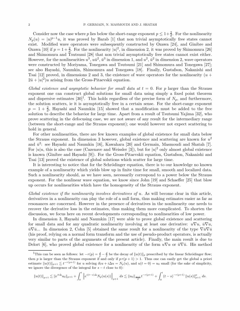
(32) h+++2 (ξ) =

∫ t

2

∫m1,0(ξ, η, σ)m0,0(ξ, η)m−1,−2(η, σ)eisϕ+++ f(σ)f(η − σ)f(ξ − η)dη dσ ds.

Using cut-off functions χ+++,Ss (ξ, η, σ) and χ+++,T

s (ξ, η, σ) adapted to ϕ+++, as explained in

Section 2.1.3, one can decompose the integral defining h+++2 . On the support of χT

s , ϕ+++ doesnot vanish, thus one can integrate by parts using

1

iϕ+++∂se

isϕ+++ = eisϕ+++ written symbolically M−2,−2∂seisϕ+++ = eisϕ+++

and obtain

h+++2 (ξ)

=

∫χ+++,Ts (ξ, η, σ)m−1,−2(ξ, η, σ)m0,0(ξ, η)m−1,−2(η, σ)eisϕ+++ f(σ)f(η − σ)f(ξ − η)dη dσ ds

]t

2

−∫ t

2

∫χ+++,Ts (ξ, η, σ)m−1,−2(ξ, η, σ)m0,0(ξ, η)m−1,−2(η, σ)

eisϕ+++ f(σ)f(η − σ)∂sf(ξ − η)dη dσ ds + {similar or easier terms}

+

∫ t

2

∫χ+++,Ss (ξ, η, σ)m1,0(ξ, η, σ)m0,0(ξ, η)m−1,−2(η, σ)eisϕ+++ f(σ)f(η − σ)f(ξ − η)dη dσ ds

def= h+++

2,1 (ξ) + h+++2,2 (ξ) + h+++

2,3 (ξ).

In particular {similar or easier terms} include the case where the time derivative hits χ+++,Ts (ξ, η, σ)

which gives a much simpler term and we will not detail it here. The terms h2,1 and h2,2 will beestimated directly; as for h2,3, its decay is not strong enough to allow for direct estimates, and we

will have to take advantage of the non-vanishing of ∂η,σϕ+++ on Suppχ+++,Ss (ξ, η, σ) and use the

identity

1

is(∂η,σϕ+++)2∂η,σϕ+++ · ∂η,σeisϕ+++ = eisϕ+++

that we write symbolically

(33)1

sM−1,−1∂η,σe

isϕ+++ = eisϕ+++.

9.3. Control of xh+++2,1 in L2. First notice that h+++

2,1 is the sum of one term evaluated at time t,and one term evaluated at time 2 ; since the term evaluated at time 2 is easy to estimate, we skipit, and focus in the following on the term corresponding to time t.

Applying ∂ξ to h+++2,1 gives terms of the type (the indices j, k, l are always non-positive)

∫mj,j−1mk,kml,l−1eitϕ+++ f(σ)f(η − σ)f(ξ − η)dη dσ with j + k + l = −3(34a)

∫tm0,−1m0,0m−1,−2eitϕ+++ f(σ)f(η − σ)f(ξ − η)dη dσ(34b)

∫m−1,−2m0,0m−1,−2eitϕ+++ f(σ)f(η − σ)∂ξ f(ξ − η)dη dσ;(34c)


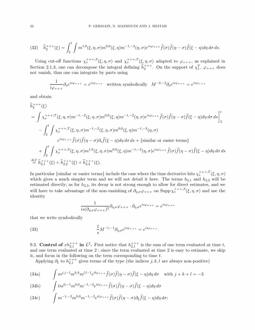
all these terms can be estimated directly with Corollary 5.6. For instance

‖(34c)‖2 =∥∥Tm−1,−2m0,0m−1,−2(e−it∆f, e−it∆f, e−it∆xf)

∥∥2

. t∥∥e−it∆f

∥∥16

∥∥e−it∆f∥∥16

∥∥e−it∆xf∥∥8/3

. ǫtt−78 t−

78 t−

14 ‖xf‖8/5 . ǫ2t−1

∥∥∥〈x〉 32 f∥∥∥2. ǫ3t−

12 .

9.4. Control of x2h+++2,1 in L2. Applying ∂ξ to h+++

2,1 gives terms of the type (the indices j, k, l

are always non-positive)∫

mj,j−1mk,kml,l−1eitϕ+++ f(σ)f(η − σ)f(ξ − η)dη dσ with j + k + l = −4(35a)

∫tmj,j−1mk,kml,l−1eitϕ+++ f(σ)f(η − σ)f(ξ − η)dη dσ with j + k + l = −2(35b)

∫mj,j−1mk,kml,l−1eitϕ+++ f(σ)f(η − σ)∂ξ f(ξ − η)dη dσ with j + k + l = −3(35c)

∫t2m1,0m0,0m−1,−2eitϕ+++ f(σ)f(η − σ)f(ξ − η)dη dσ(35d)

∫tm0,−1m0,0m−1,−2eitϕ+++ f(σ)f(η − σ)∂ξ f(ξ − η)dη dσ(35e)

∫m−1,−2m0,0m−1,−2eitϕ+++ f(σ)f(η − σ)∂2

ξ f(ξ − η)dη dσ;(35f)

all these terms can be estimated directly with Corollary 5.6, except for the last one, which requiresa further manipulation; indeed, the Lebesgue exponents ∞, ∞, 2 are not allowed by Corollary 5.6for the arguments of the multilinear operator.

Thus one writes ∂2ξ f(ξ − η) = −∂η∂ξ f(ξ − η), and integrates by parts in η. This yields terms of

type (35c) and (35e), as well as

(36)

∫m−1,−2m0,0m−1,−2eitϕ+++ f(σ)∂η f(η − σ)∂ξ f(ξ − η)dη dσ

which can be estimated as follows

‖(36)‖2 =∥∥Tm−1,−2m0,0m−1,−2(e−it∆f, e−it∆xf, e−it∆xf)

∥∥2

. t∥∥e−it∆f

∥∥32

∥∥e−it∆f∥∥32/14

∥∥e−it∆xf∥∥32

. t ‖xf‖32/31 t−1516 ‖xf‖32/18 t−

18 ǫt−

1516

. t∥∥〈x2〉f

∥∥2t−

1516

∥∥∥〈|x|5/4〉f∥∥∥2t−

18 ǫt−

1516

. ǫ3t t t−1516 t1/4t−

18 t−

1516 . ǫ3t1/8.

9.5. Control of e−it∆h+++2,1 in L∞. This control would be very easily obtained if pseudo-product

operators were bounded with values in L∞. Since this is not the case, we use Sobolev inequality,namely

||e−it∆h+++2,1 ||L∞ ≤ ||e−it∆h+++

2,1 ||W 1,8

≤ ||Tm−1,−1m0,0m−1,−2(e−it∆f, e−it∆f, e−it∆f)||L8

≤ t||e−it∆f ||3L24 ≤ ǫ31

t

1

t3/4

where we have used that m−1,−2 + ξm−1,−2 = m−1,−1.


9.6. Control of xh+++2,2 in L2. Applying ∂ξ to h2,2(ξ) gives terms of the type (the indices j, k, l

are always non-positive)∫ t

2

∫mj,j−1mk,kml,l−1eisϕ+++ f(σ)f(η − σ)∂sf(ξ − η)dη dσ ds with j + k + l = −3(37a)

∫ t

2

∫sm0,−1m0,0m−1,−2eisϕ+++ f(σ)f(η − σ)∂sf(ξ − η)dη dσ ds(37b)

∫ t

2

∫m−1,−2m0,0m−1,−2eisϕ+++ f(σ)f (η − σ)∂ξ∂sf(ξ − η)dη dσ ds.(37c)

We now transform (37c) by observing that ∂ξ∂sf(ξ − η) = −∂η∂sf(ξ − η) and integrating by partsin η. This gives terms of type (37a) (37b) as well as

(38)

∫ t

2

∫m−1,−2m0,0m−1,−2eisϕ+++ f(σ)∂η f(η − σ)∂sf(ξ − η)dη dσ ds.

Actually, terms like (38) can also come from the {similar or easier terms} in the definition of h+++2,2 .

Now the terms (37a) (37b) (38) are easily estimated by using Corollary 5.6 and (1). For instance

‖(37a)‖2 ≤∫ t

2

∥∥eis∆Tmj,j−1mk,kml,l−1(e−is∆f, e−is∆f, e−is∆∂sf)∥∥2ds

=

∫ t

2

∥∥Tmj,j−1mk,kml,l−1(e−is∆f, e−is∆f,Q(u, u) +Q(u, u)∥∥2ds

.

∫ t

2s3/2‖e−is∆f‖48 ds .

∫ t

2ǫ4s3/2(s−3/4)4 ds . ǫ4.

(39)

9.7. Control of x2h+++2,2 in L2. We saw that xh+++

2,2 can be reduced to terms of the type (37a)

(37b) (38). Now apply ∂ξ to (37a) (37b) (38), and, as in Section 9.6, make sure by an integrationby parts if necessary that an s derivative and a ξ derivative do not hit the same f . This gives termsof the types (the indices j, k, l are always non-positive)

∫ t

2

∫mj,j−1mk,kml,l−1eisϕ+++ f(σ)f(η − σ)∂sf(ξ − η)dη dσ ds with j + k + l = −4(40a)

∫ t

2

∫s2m1,0m0,0m−1,−2eisϕ+++ f(σ)f(η − σ)∂sf(ξ − η)dη dσ ds(40b)

∫ t

2

∫m−1,−2m0,0m−1,−2eisϕ+++ f(σ)∂2

η f(η − σ)∂sf(ξ − η)dη dσ ds(40c)

∫ t

2

∫smj,j−1mk,kml,l−1eisϕ+++ f(σ)f(η − σ)∂sf(ξ − η)dη dσ ds with j + k + l = −2(40d)

∫ t

2

∫smj,j−1mk,kml,l−1eisϕ+++ f(σ)∂η f(η − σ)∂sf(ξ − η)dη dσ ds with j + k + l = −1(40e)

∫ t

2

∫mj,j−1mk,kml,l−1eisϕ+++ f(σ)∂η f(η − σ)∂sf(ξ − η)dη dσ ds with j + k + l = −3.(40f)

In order to bound the terms above, one should notice first that e−it∆∂sf = αQ(u, u) + βQ(u, u),hence ∥∥e−it∆∂sf

∥∥p. ǫ2t

2p−2 for 2 ≤ p < ∞.

The estimates for (40a)-(40f) follow in a straightforward fashion using Corollary 5.6, except for (40c).


But for (40c), writing ∂2η f(η − σ) = −∂η∂σ f(η − σ), and integrating by parts gives, in addition

to already treated terms,

(41)

∫ t

2

∫m−1,−2m0,0m−1,−2eisϕ+++∂σ f(σ)∂η f(η − σ)∂sf(ξ − η)dη dσ ds,

which can be treated directly:

‖(41)‖2 .∫ t

2

∥∥Tm−1,−2m0,0m−1,−2

(e−it∆xf, e−it∆xf, e−it∆∂sf

)∥∥2ds

.

∫ t

2s∥∥e−it∆xf

∥∥232/7

∥∥e−it∆∂sf∥∥16

ds .

∫ t

2s(s−9/16 ‖xf‖32/25

)2ǫ2s−15/8 ds

.

∫ t

2s(s−9/16

∥∥∥〈x〉13/8f∥∥∥2

)2ǫ2s−15/8 ds . ǫ4

∫ t

2s(s−9/16s5/8

)2s−15/8 ds . ǫ4t1/4.

(42)

9.8. Control of e−it∆h+++2,2 in L∞. Proceeding as in Section 8.4, we rewrite

h+++2,2 =

∫ t−1

2eis∆H1

2,2(s) ds+

∫ t

t−1H2

2,2(s) ds,

where{

H12,2(ξ, s)

def=∫m−1,−2(ξ, η, σ)m0,0(ξ, η)m−1,−2(η, σ)eisϕ+++ f(σ)f(η − σ)∂sf(ξ − η)dη dσ

H22,2(ξ, s)

def=∫m−1,−2(ξ, η, σ)m0,0(ξ, η)m−1,−2(η, σ)eisϕ+++ f(σ)f(η − σ)∂sf(ξ − η)dη dσ

with

ϕ+++(ξ, η) = |ξ − η|2 + |η − σ|2 + |σ|2.Then

e−it∆h+++2,2 =e−it∆

∫ t−1

2eis∆H1

2,2(s) ds(43a)

+ e−it∆

∫ t

t−1H2

2,2(s) ds.(43b)

9.8.1. Estimate of (43a). On the one hand, one sees immediately that

(44) ‖H12,2(s)‖2 =

∥∥Tm−1,−2m0,0m−1,−2(e−is∆f, e−is∆f, e−is∆∂sf)∥∥2.

1

s2

On the other hand, proceeding as in Section 9.6, we can write ∂ξH12,2 as a sum of terms of the type

(the indices j, k, l are always non-positive)∫

mj,j−1mk,kml,l−1eisϕ+++ f(σ)f(η − σ)∂sf(ξ − η)dη dσ with j + k + l = −3(45a)

∫sm0,−1m0,0m−1,−2eisϕ+++ f(σ)f(η − σ)∂sf(ξ − η)dη dσ(45b)

∫m−1,−2m0,0m−1,−2eisϕ+++ f(σ)∂σ f(η − σ)∂sf(ξ − η)dη dσ.(45c)

Let us focus for instance on (45a). It can be estimated in L8/5 as follows:

‖(45a)‖8/5 =∥∥Tmj,j−1mk,kml,l−1(e−is∆f, e−is∆f, e−is∆∂sf)

∥∥8/5

. s3/2‖e−is∆f‖16‖f‖16‖∂sf‖2 . ǫ4s3/2s−7/8s−7/8 1

s.

ǫ4

s5/4.

(46)


Estimating similarly (29b) (29c), we get

(47) ‖xH12,2(s)‖8/5 .

ǫ4

s5/4.

Putting together (44) and (47) gives

‖H12,2(s)‖1 . ‖H1

2,2(s)‖2 + ‖xH12,2(s)‖8/5 .

ǫ4

s5/4.

Therefore

‖(43a)‖∞ =

∥∥∥∥∫ t−1

2ei(s−t)∆H1

2,2(s) ds

∥∥∥∥∞

.

∫ t

2

1

t− s‖H2,2(s)‖1 ds

. ǫ4∫ t

2

1

t− s

1

s5/4ds .

ǫ4

t.

(48)

9.8.2. Estimate of (43b). Proceeding as in section (9.7), one sees that

‖〈x〉2H22,2‖2 .

ǫ4√t.

Therefore,

‖(43b)‖∞ =

∥∥∥∥e−it∆

∫ t

t−1H2

2,2(s) ds

∥∥∥∥∞

.1

t

∥∥∥∥∫ t

t−1H2

2,2(s) ds

∥∥∥∥1

.ǫ4

t√t.(49)

9.9. Control of xh+++2,3 in L2. Applying ∂ξ to h+++

2,3 (ξ), one gets terms of the types (the indices

j, k, l are always non-positive)

∫ t

2

∫m1,0mk,kml,l−1eisϕ+++ f(σ)f(η − σ)f(ξ − η)dη dσ ds with k + l = −2(50a)

∫ t

2

∫mj,j−1mk,kml,l−1eisϕ+++ f(σ)f (η − σ)f(ξ − η)dη dσ ds with j + k + l = −1(50b)

∫ t

2

∫m1,0m0,0m−1,−2eisϕ+++ f(σ)f(η − σ)∂ξ f(ξ − η)dη dσ ds(50c)

∫ t

2

∫sm2,1m0,0m−1,−2eisϕ+++ f(σ)f(η − σ)f(ξ − η)dη dσ ds.(50d)

The terms (50b) and (50c) can be estimated in a straightforward fashion using Corollary 5.6. Usingthe identity (33) to transform the last term above, we see that it can be reduced to terms of thetype (50a) (50b) (50c). Finally, using (33) to transform (50a) yields terms of type (the indices j, k, lare always non-positive)

∫ t

2

∫1

smj,j−1mk,kml,l−1eisϕ+++∂σ f(σ)f(η − σ)f(ξ − η)dη dσ ds with j + k + l = −2(51a)

∫ t

2

∫1

smj,j−1mk,kml,l−1eisϕ+++ f(σ)f(η − σ)f(ξ − η)dη dσ ds with j + k + l = −3;(51b)

these terms can be estimated directly using Corollary 5.6.

9.10. Control of e−it∆h+++2,3 in L∞. This can be done as in sections 8.4 and 9.8.


9.11. Control of x2h+++2,3 in L2. We saw in Section 9.9 that xh+++

2,3 can be reduced to terms of the

form (50b) (50c) (51a) (51b). Applying ∂ξ to (50b) (50c) (51a) (51b) gives terms of the followingtypes (the indices j, k, l are always non-positive)

∫ t

2

∫mj,j−1mk,kml,l−1eisϕ+++ f(σ)f(η − σ)f(ξ − η)dη dσ ds with j + k + l = −2(52a)

∫ t

2

∫sm1,0mk,kml,l−1eisϕ+++ f(σ)f (η − σ)f(ξ − η)dη dσ ds with j + k + l = −1(52b)

∫ t

2

∫mj,j−1mk,kml,l−1eisϕ+++ f(σ)f(η − σ)∂ξ f(ξ − η)dη dσ ds with j + k + l = −1(52c)

∫ t

2

∫m1,0mk,kml,l−1eisϕ+++ f(σ)f(η − σ)∂ξ f(ξ − η)dη dσ ds with j + k + l = −2(52d)

∫ t

2

∫sm2,1m0,0m−1,−2eisϕ+++ f(σ)f (η − σ)∂ξ f(ξ − η)dη dσ ds(52e)

∫ t

2

∫m1,0m0,0m−1,−2eisϕ+++ f(σ)f(η − σ)∂2

ξ f(ξ − η)dη dσ ds(52f)

∫ t

2

∫1

smj,j−1mk,kml,l−1eisϕ+++∂σ f(σ)f(η − σ)f(ξ − η)dη dσ ds with j + k + l = −3(52g)

∫ t

2

∫mj,j−1mk,kml,l−1eisϕ+++∂σ f(σ)f (η − σ)f(ξ − η)dη dσ ds with j + k + l = −1(52h)

∫ t

2

∫1

smj,j−1mk,kml,l−1eisϕ+++∂σ f(σ)f(η − σ)∂ξ f(ξ − η)dη dσ ds with j + k + l = −2(52i)

∫ t

2

∫1

smj,j−1mk,kml,l−1eisϕ+++ f(σ)f(η − σ)f(ξ − η)dη dσ ds with j + k + l = −4(52j)

∫ t

2

∫mj,j−1mk,kml,l−1eisϕ+++ f(σ)f(η − σ)f(ξ − η)dη dσ ds with j + k + l = −2.(52k)

These terms can be bounded in a similar way to all the estimates already performed, except fortwo of them: (52e) and (52f). Since the former can be reduced to the latter by integration by partsusing (33), we shall focus on (52f), the difficulty being that the L∞×L∞ ×L2 → L2 estimate doesnot hold in general for flag singularity paraproducts; to go around it, we shall use (ii) in Theorem 3.

First observe that the case where |ξ| . |η, σ| can be easily dealt with, for then the symbolm1,0(ξ, η, σ)m0,0(ξ, η)m−1,−2(η, σ) becomes m0,−2(ξ, η, σ)m0,0(ξ, η). Thus we shall assume that|ξ| >> |η, σ|. Next, by symmetry, it is possible to assume that in the integral defining (52f),|σ| & |η − σ|. Thus it suffices to consider the case |ξ| >> |σ| & |η − σ|. As usual, this can beensured by adding a cut-off function, which we denote χ(ξ, η, σ). Finally notice that the condition|σ| & |η − σ| imposes |σ| & 1√

son the support of m−1,−2(σ, η − σ). We now decompose

∫ t

2

∫m1,0m0,0m−1,−2χ(η, σ)eisϕ+++ f(σ)f(η − σ)∂2

ξ f(ξ − η)dη dσ ds

=

∫ t

2

∫ ∑

2j& 1√s

2−jm1,0m0,0m0,−1χ(η, σ)eisϕ+++

× θ( σ

2j

)f(σ)Θ

(η − σ

4 · 2j)f(η − σ)∂2

ξ f(ξ − η)dη dσ ds.

(53)


This can be estimated by (ii) of Theorem 3:

‖(53)‖2 .∫ t

2

∑

2j& 1√s

2−j∥∥Tm1,0m0,0m0,−1

(Pje

is∆f, P<j+2eis∆f, eis∆x2f

)∥∥2ds

.

∫ t

2

∑

2j& 1√s

2−j∥∥eis∆f

∥∥∞∥∥eis∆f

∥∥∞∥∥x2f

∥∥2ds .

∫ t

2ǫ3√s1

s

1

ss ds . ǫ3

√t.

10. Estimates on h3

From its definition in section 2.2, we see that h3 can be written as

h3(ξ) = h+++3 (ξ) + h+−−

3 (ξ) + h−−−3 (ξ) + h−++

3 (ξ)

with

(54) h±±±3 (ξ) =

∫ t

2

∫q(η, σ)m−1,−2(ξ, η)eisϕ±±± f(σ)f(η − σ)f(ξ − η) dη dσ ds.

Observe (as in Section 9) that the symbol q(η, σ)m−1,−2(ξ, η) can be writtenm1,0(ξ, η, σ)m−1,−2(ξ, η).

10.1. The cases + + +, + − − and − − −. Notice (see Section 2.1.2) that the three phasesϕ = ϕ+++, ϕ+−−, ϕ−−− correspond to a space-time resonant set R = {ϕ = 0} ∪ {∂η,σϕ = 0} ={ξ = η = 0}. Thus one can proceed as in Section 9 to derive the desired estimates in most cases.Only one term has to be treated in a different way. It occurs when estimating x2h+++

2 (we focusfrom now on on the + + + case), corresponds to (52f), and reads

∫ t

2

∫m1,0(ξ, η, σ)m−1,−2(ξ, η)eisϕ+++ f(σ)f(η − σ)∂2


In order to estimate it, one has to distinguish between the cases |η| >> |ξ − η| and |η| . |ξ − η|.Since they are fairly similar, we shall focus on the former; as usual this is ensured by adding acut-off function χ which localizes frequencies to this set, thus we now consider

(55)

∫ t

2

∫m1,0(ξ, η, σ)m−1,−2(ξ, η)χ(ξ, η)eisϕ+++ f(σ)f (η − σ)∂2



Observe that |η| >> |ξ−η| implies |ξ−η| << |ξ|; and also that the support condition onm−1,−2s (ξ, η)

implies |ξ| & 1√s. Therefore, we can estimate, with the help of Bernstein’s lemma

‖(55)‖2 .∑

j

‖Pj(55)‖2

=

∥∥∥∥∥∥∑

j

Pj

∫ t

2

∫ t

2Tm1,0m−1,−2χ(ξ,η)

(eis∆f , eis∆f , P<j+1e

is∆x2f)ds

∥∥∥∥∥∥2

.

∫ t

2

∑

2j& 1√s

2−j∥∥Tm1,0m0,−1

(eis∆f , eis∆f , P<j+1e

is∆x2f)∥∥

2ds

.

∫ t

2

∑

2j& 1√s

2−j∥∥eis∆f

∥∥16

∥∥eis∆f∥∥16

∥∥eis∆P<j+1x2f∥∥8/3

ds

. ǫ2∫ t

2

∑

2j& 1√s

2−js−7/8s−7/82j/4‖x2f‖2 ds

. ǫ3∫ t

2s3/8s−7/8s−7/8s ds . ǫ3t5/8.

10.2. The case − + +. In the case of ϕ−++, the space-time resonant set R−++ = {ξ = σ = 12η}

(see (2.1.2) is not reduced to the origin. Using an appropriate (smooth, homogeneous of degree 0)cut-off function χ−++, one can restrict the problem to a neighbourhood of R−++, the rest beingtreated as in Section 9. Furthermore, this neigbourhood is chosen such that ξ, η, σ essentially havethe same size. This has the advantage of canceling the flag singularity, in other words the abovesymbol χ−++(ξ, η, σ)m

1,0(ξ, η, σ)m−1,−2(ξ, η) can be replaced by χ−++(ξ, η, σ)m0,−2(ξ, η, σ).

In the following of this section, we will thus consider the term obtained after restricting ξ, η, σto a neighbourhood of R−++:

(56)h−++

3 (ξ) =

∫ t

2

∫χ−++(ξ, η, σ)m

0,−2(ξ, η, σ)eisϕ−++ f(σ)f(η − σ)f(ξ − η) dη dσ ds.

10.3. Control of h−++3 in L2. Immediate.

10.4. Control of xh−++3 in L2. Applying ∂ξ to

h−++

3 gives∫ t

2

∫χ−++(ξ, η, σ)m

−1,−3(ξ, η, σ)eisϕ−++ f(σ)f(η − σ)f(ξ − η) dη dσ ds(57a)

+

∫ t

2

∫χ−++(ξ, η, σ)m

0,−2(ξ, η, σ)eisϕ−++∂ξ f(σ)f (η − σ)f(ξ − η) dη dσ ds(57b)

+

∫ t

2

∫χ−++(ξ, η, σ)m

0,−2(ξ, η, σ)s∂ξϕ−++eisϕ−++ f(σ)f(η − σ)f(ξ − η) dη dσ ds.(57c)

The term (57a) and (57b) can be estimated without any difficulty by Corollary 5.6. For (57c), weuse the following relation:

∂ξϕ−++ = −2∂ηϕ−++ − ∂σϕ−++.

Substituting the above right-hand side for ∂ξϕ−++ in (57c), we can integrate this term by partsusing the relations

s∂ηϕ−++eisϕ−++ =

1

i∂ηe

isϕ−++ and s∂σϕ−++eisϕ−++ =

1

i∂σe

isϕ−++,


and the result is terms of the form (57a) and (57b)

10.5. Control of e−it∆h−++3 in L∞. Our strategy will be the following: by the standard dispersive

estimate, the decay of e−it∆h−++3 in L∞ follows from a bound on

∥∥∥h−++3

∥∥∥1. The quantity whose

control was obtained in the previous paragraph, namely∥∥∥xh−++

3

∥∥∥2barely fails to control

∥∥∥h−++3

∥∥∥1,

but it will suffice to obtain a control of this weighted norm with a Lebesgue index slightly smallerthan 2.

To this we now turn: we will prove that∥∥∥xh−++

3

∥∥∥8/5

remains bounded, and, as explained above,

this will give us the desired result since∥∥∥e−it∆h−++

3

∥∥∥∞

.1

t

∥∥∥h−++3

∥∥∥1.

1

t

(∥∥∥h−++3

∥∥∥2+∥∥∥xh−++

3

∥∥∥8/5

).

We saw in the previous paragraph that xh−++3 can be written as a sum of the terms of the

type (57a) or (57b). We will show how to obtain a bound for terms of the type (57b), the caseof (57a) can be treated in an identical fashion.

Next observe that one can write

Bχ−++(ξ,η,σ)m0,−2(ξ,η,σ) = P<− 12log sBm0,0(ξ,η,σ) +

∑

− 12log s<j

inf(1, 2−2j)PjBm0.0(ξ,η,σ).

Therefore, using in addition to the traditional arguments the point (iv) of Lemma 4.2 gives∥∥∥xh−++

3

∥∥∥8/5

=

∥∥∥∥∫ t

0eis∆Bχ−++(ξ,η,σ)m0,−2(ξ,η,σ)

(e−is∆f, e−is∆f, e−is∆xf

)∥∥∥∥8/5

.

∫ t

0

[ ∥∥∥P<− 12log se

is∆Bχ−++(ξ,η,σ)m0,0(ξ,η,σ)


)∥∥∥8/5

+∑

j>− 12log s

inf(1, 2−2j)∥∥PjBm0.0(ξ,η,σ)


)∥∥8/5

]ds

.

∫ t

0

[‖u(s)‖16 ‖u(s)‖16 ‖xf‖2 +

∑

j>− 12log s

inf(1, 2−2j)2j/4t1/8 ‖u(s)‖16 ‖u(s)‖16 ‖xf‖2]ds

. ǫ3∫ t

0

[s−7/8s−7/8 +

∑

j>− 12log s

inf(1, 2−2j)2j/4s1/8s−7/8s−7/8]ds . ǫ3.

10.6. Control of x2h−++3 in L2. We saw in Section 10.4 that xh−++

3 could be reduced to theterms (57a) and (57b). Applying ∂ξ to these two terms gives expressions of the following types

∫ t

2

∫m−2,−4(ξ, η, σ)eisϕ−++ f(σ)f(η − σ)f(ξ − η) dη dσ ds(58a)

∫ t

2

∫m−1,−3(ξ, η, σ)eisϕ−++ f(σ)f(η − σ)∂ξ f(ξ − η) dη dσ ds(58b)

∫ t

2s

∫m0,−2(ξ, η, σ)eisϕ−++ f(σ)f(η − σ)f(ξ − η) dη dσ ds(58c)

∫ t

2s

∫m1,−1(ξ, η, σ)eisϕ−++ f(σ)f(η − σ)∂ξ f(ξ − η) dη dσ ds(58d)

∫ t

2

∫m0,−2(ξ, η, σ)eisϕ−++ f(σ)f(η − σ)∂2

ξ f(ξ − η) dη dσ ds.(58e)


All these expressions can be estimated directly with the help of Corollary 5.6.

Appendix A. Proof of Theorem 3

We shall only prove (i) in Theorem 3: if m is of flag singularity type with degree 0, then theoperator

Tm : Lp × Lq × Lr → Ls

is bounded for1

s=

1

p+

1

q+

1

rif 1 < p, q, r, s < ∞

with a bound less than a multiple of ‖m‖FS , and this result remains true if s = 2 and only one ofp, q, r is taken equal to ∞.

The proof of (ii) follows the steps of (i), but is much simpler, thus we shall skip it.

Remark. It would be of particular interest for the PDE problem which is the heart of the presentpaper to obtain estimates of the type L∞×L∞×L2 → L2. This set of Lebesgue indices is not coveredby Theorem 3, unless a projection P0 on a band of frequencies is added. To see that boundednessfor this choice of spaces does not hold in general, take B a bilinear Coifman-Meyer operator, andform the flag singularity pseudo-product operator

Tdef: (f1, f2, f3) 7→ B(f1, f2)f3.

The operator T is bounded from L∞ × L∞ × L2 to L2 if and only if B is bounded from L∞ × L∞

to L∞; but this last property is not true for general Coifman-Meyer operators.

We now start with the proof of Theorem 3:Step 1: partition of the (ξ, η, σ) plane By definition of a flag singularity with degree 0, the symbolm can be written

mIII(ξ, η, σ)mII1 (η, ξ)mII

2 (η, σ),

with mIII , mII1 and mII

2 of Coifman-Meyer type. First observe that there are certain regionsof the (ξ, η, σ) plane where m satisfies the Coifman-Meyer estimates (12); hence the Coifman-Meyer theorem applies, and the desired estimate is proved. Thus, using a (homogeneous of degree0, smooth away from 0) cut-off function, we can reduce the problem to the regions where theCoifman-Meyer estimate (12) does not hold for m, namely

A1 ∪A2def= {|ξ|+ |η| ≤ ǫ|σ|} ∪ {|η| + |σ| ≤ ǫ|ξ|},

where ǫ is a small constant. We further observe that on A1 (respectively: on A2), mII2 (respectively

mII1 ) satisfies the Coifman-Meyer estimate in (ξ, η, σ). Now choose cut-off functions χA1(ξ, η, σ)

and χA2(ξ, η, σ) which have homogeneous bounds of degree 0, and localize respectively near A1 andA2. More precisely, we choose χA1 such that

TχA1(ξ,η,σ)(f1, f2, f3) =

∑

k

P<k−100 (Pkf1Pkf2)P<k−100f3,

and similarly for χA2 . With the help of these cutoff functions, we can reduce matters to symbolsof the two following types:

χA1(ξ, η, σ)mIII (ξ, η, σ)mII

1 (η, ξ)

χA2(ξ, η, σ)mIII (ξ, η, σ)mII

2 (η, σ)(A.1)

Observe that, 〈·, ·〉 denoting the standard scalar product,

〈Tµ(ξ,η,σ)ν(η,σ)(f1, f2, f3) , f4〉 = 〈Tµ(σ,η,ξ)ν(η,ξ)(f4, f3(−·), f2(−·)) , f1〉.thus estimates for one of the above symbols can be deduced from the other by duality if all theLebesgue indices are finite.


We focus from now on symbols of the first type in (A.1).

Step 2: series expansion of mIII Let us expand in series the symbol mIII(ξ, η, σ) around (η, ξ) = 0.One gets

mIII(ξ, η, σ) =M−1∑

|α|=0

Φα(σ)(η, ξ)α +R(ξ, η, σ),

where Φα(σ) =∂α

∂(ξ,η)αmIII(0, 0, σ) and the remainder R satisfies

(A.2)∣∣∣∂β

η,ξ∂γσR(ξ, η, σ)

∣∣∣ = O

((|ξ|+ |η|)M−|β|

|σ|M+|α|

).

Coming back to the original symbol (A.1), we see that

χA1(ξ, η, σ)mIII(ξ, η, σ)mII

1 (η, ξ)

= χA1(ξ, η, σ)

M−1∑

|α|=0

Φα(σ)mII1 (η, ξ)(η, ξ)α + χA1(ξ, η, σ)R(ξ, η, σ)mII

1 (η, ξ).

ChoosingM big enough, the bounds (A.2) satisfied byR let the symbol χA1(ξ, η, σ)R(ξ, η, σ)mII1 (η, ξ)

satisfy Coifman-Meyer estimates, hence the associated operator enjoys the desired bounds. Thus itsuffices to treat the summands of the first term of the above right-hand side; to simplify notationsa little in the following, we replace (ξ, η)α by (ξ − η)α, and consider therefore symbols of the type

(A.3) χA1(ξ, η, σ)Φα(σ)(ξ, η)αm(η, ξ),

where Φα is homogeneous of degree −|α|, and m has homogeneous bounds of degree 0.

Step 3: paraproduct decomposition of m Recall that m is a symbol with homogeneous bounds ofdegree 0, defined at the end of the last paragraph. Its paraproduct decomposition reads

Bm(f, g) =∑

j

Bm(Pjf, P<j−1g) +∑

j

Bm(P<j−1f, Pjg) +∑

|j−k|≤1

Bm(Pjf, Pkg).

Proceeding as in the original work of Coifman-Meyer [4], consider the symbol of one of the elemen-tary bilinear operators above, for instance Bm(Pj ·, P<j−1·). Denote by mj(ξ, η) this symbol, whichis compactly supported (in (ξ, η)), and expand it in Fourier series

mj(ξ, η) = χ(ξ, η)∑

p,q∈Z2

ajp,qeic2−j(p,q)·(ξ,η),

where we denoted c for a constant, χ for a cut-off function, and ajp,q for the Fourier coefficients.It is now possible to forget about the summation over p, q. The idea is that the fast decay of the

ajp,q (in p, q), due to the smoothness of the symbol, offsets the polynomial factors arising from the

complex exponentials eic2−j(p,q), which correspond to translations in physical space. Les us be a bit

more explicit about this: we will in the following be using maximal and square function estimates.As far as maximal functions are concerned, there holds | [S<jf ] (x + 2−jq)| . |q|2|Mf(x)|, whichis the announced polynomial growth. As far as square functions are concerned, we rely on theboundedness of operators of the type f 7→ ∑

j αj [Pjf ](x + q2−j) on Lp spaces with p < ∞, ifαj ∈ ℓ∞. The bounds of these operators grow polynomially in q.

These considerations reduce matters to the case wherem is given by one of the three paraproductoperators

(f, g) 7→∑

j

PjfP<j−1g ;∑

j

P<j−1fPjg ;∑

j

PjfPjg

(we suppressed the index k in the last summation to make notations lighter).


Step 4: derivation of the model operators Combining this last line with (A.3), we see that the op-erators of interest for us become

∑

j,k

P<k−100Pj (Φi(D)Pkf1Pkf2)∇iP<j−1P<k−100f3

∑

j,k

P<k−100P<j−1 (Φi(D)Pkf1Pkf2)∇iPjP<k−100f3

∑

j,k

P<k−100Pj (Φi(D)Pkf1Pkf2)∇iPjP<k−100f3.

(A.4)

where here i = |α| and ∇i stands for ∇α. We now make some observations which allow us tosimplify the above operators:

• First remark that Φi(D)Pk, ∇iPj and ∇iP<j can be written respectively 2−ikPk, 2ij ˜P j and

2ijP<j with obvious notations. Since the operators with tildes have very close propertiesto the operators without tildes, we will in the following forget about the tildes.

• Next notice that due to the Fourier space support properties of the different terms above,it is possible to restrict the summation to j ≤ k − 97.

• Finally, since P<k−100Pj = Pj and P<j−1P<k−100 = P<j−1 for j ≤ k− 103, it is harmless toforget about the P<k−100 operators in the above sums.

All these remarks lead to the following simplified versions of the above operators:

∑

k≥j+97

2i(j−k)Pj (Pkf1Pkf2)P<j−1f3(A.5a)

∑

k≥j+97

2i(j−k)P<j−1 (Pkf1Pkf2)Pjf3(A.5b)

∑

k≥j+97

2i(j−k)Pj (Pkf1Pkf2)Pjf3(A.5c)

Step 5: the case i = 0 If i = 0, observe that, due to the Fourier support properties of the Littlewood-Paley operators, the operators in (A.5a) and (A.5c) are equal respectively to

∑

j

Pj

(∑

k

Pkf1Pkf2

)P<j−1f3

∑

j

Pj

(∑

k

Pkf1Pkf2

)Pjf3

(A.6)

up to a difference term which is Coifman-Meyer. But the operators in (A.6) are simply compositionsof bilinear Coifman-Meyer operators. Thus the desired bounds follow for them.


The operator in (A.5b) can be estimated with the help of the Littlewood-Paley square andmaximal function estimates (Theorem 2):

‖(A.5b)‖s .

∥∥∥∥∥∥∥

∑

j

P<j−1

∑

k≥j+97

Pkf1Pkf2

Pjf3

2

1/2∥∥∥∥∥∥∥s

.

∥∥∥∥∥∥∥

∑

j

[Pjf3]2

1/2

supj

∣∣∣∣∣∣P<j−1

∑

k≥j+97

Pkf1Pkf2

∣∣∣∣∣∣

∥∥∥∥∥∥∥s

. ‖Sf3‖r

∥∥∥∥∥∥M

sup

j

∣∣∣∣∣∣∑

k≥j+97

Pkf1Pkf2

∣∣∣∣∣∣

∥∥∥∥∥∥

srs−r

. ‖f3‖r ‖M (Sf1Sf2)‖ srs−r

. ‖f3‖r ‖Sf1Sf2‖ srs−r

. ‖f3‖r ‖Sf1‖p ‖Sf2‖q .

Step 6: the case i > 0 If i > 0, we see that it suffices to prove uniform estimates in J ≥ 0 for theoperators

∑

j

Pj (Pj+Jf1Pj+Jf2)P<j−1f3(A.7a)

∑

j

P<j−1 (Pj+Jf1Pj+Jf2)Pjf3(A.7b)

∑

j

Pj (Pj+Jf1Pj+Jf2)Pjf3(A.7c)

since the desired result follows then upon summation over J . We start with the case where allthe Lebesgue indices are finite. The estimate relies on the Littlewood-Paley square and maximalfunction estimates (Theorem 2), and on the vector valued maximal function estimate (see Stein [29],chapter II) ∥∥∥∥∥∥∥

∑

j

[Mfj]2

1/2∥∥∥∥∥∥∥p

.

∥∥∥∥∥∥∥

∑

j

f2j

1/2∥∥∥∥∥∥∥p

This gives for (A.7a)

‖(A.7a)‖s .

∥∥∥∥∥∥∥

∑

j

[Pj (Pj+Jf1Pj+Jf2)P<j−1f3]2

1/2∥∥∥∥∥∥∥s

.

∥∥∥∥∥∥∥Mf3

∑

j

[Pj (Pj+Jf1Pj+Jf2)]2

1/2∥∥∥∥∥∥∥s

. ‖Mf3‖r

∥∥∥∥∥∥∥

∑

j


1/2∥∥∥∥∥∥∥

srs−r

. ‖f3‖r

∥∥∥∥∥∥∥

∑

j

[M (Pj+Jf1Pj+Jf2)]2

1/2∥∥∥∥∥∥∥

srs−r

. ‖f3‖r

∥∥∥∥∥∥∥

∑

j

[Pj+Jf1Pj+Jf2]2

1/2∥∥∥∥∥∥∥

srs−r

. ‖f3‖r

∥∥∥∥∥∥∥Mf1

∑

j

[Pj+Jf2]2

1/2∥∥∥∥∥∥∥

srs−r

. ‖f3‖r ‖Mf1‖p ‖Sf2‖q . ‖f3‖r ‖f1‖p ‖f2‖q .


(A.7c) is estimated similarly

‖(A.7c)‖s .

∥∥∥∥∥∥∥

∑

j


1/2∑

j

[Pjf3]2

1/2∥∥∥∥∥∥∥s

.

∥∥∥∥∥∥∥

∑

j


1/2∥∥∥∥∥∥∥

srs−r

∥∥∥∥∥∥∑

j

[Pjf3]2

∥∥∥∥∥∥

2

r

. ‖f1‖p ‖f2‖q ‖f3‖2 .And finally (A.7b):

‖(A.7b)‖s .

∥∥∥∥∥∥∥

∑

j

[P<j−1 (Pj+Jf1Pj+Jf2)Pjf3]2

1/2∥∥∥∥∥∥∥s

.

∥∥∥∥∥supj[P<j−1 (Pj+Jf1Pj+Jf2)]

∥∥∥∥∥srs−r

∥∥∥∥∥∥∥

∑

j

[Pjf3]2

1/2∥∥∥∥∥∥∥r

. ‖M (Mf1Mf2)‖ srs−r

‖Sf3‖r . ‖Mf1Mf2‖ srs−r

‖f3‖r. ‖Mf1‖p ‖Mf2‖q ‖f3‖r . ‖f1‖p ‖f2‖q ‖f3‖r .

References

[1] Barab, J., Nonexistence of asymptotically free solutions for a nonlinear Schrodinger equation. J. Math. Phys.25 (1984), no. 11, 3270–3273.

[2] Cazenave, T., Semilinear Schrodinger equations. Courant Lecture Notes in Mathematics, 10. New York Uni-versity, Courant Institute of Mathematical Sciences, New York; American Mathematical Society, Providence,RI, 2003

[3] Cazenave, T; Weissler, F, Rapidly decaying solutions of the nonlinear Schrodinger equation. Comm. Math.Phys. 147 (1992), no. 1, 75–100.

[4] Coifman, R.; Meyer, Y., Au dela des operateurs pseudo-differentiels. Asterisque, 57. Societe Mathematique deFrance, Paris, 1978.

[5] Cohn, S., Resonance and long time existence for the quadratic semilinear Schrodinger equation. Comm. PureAppl. Math. 45 (1992), no. 8, 973–1001.

[6] Delort, J.-M., Global solutions for small nonlinear long range perturbations of two dimensional Schrodinger

equations. Mem. Soc. Math. Fr. (N.S.) 91 (2002).[7] Germain, P., Masmoudi, N., Shatah, J., Global solutions for 3D quadratic Schrodinger equations, accepted by

International Mathematics Research Notices.[8] Germain, P., Masmoudi, N., Shatah, J., Global solutions for the gravity water wave equations in dimension 3,

preprint.[9] Ginibre, J.; Hayashi, N., Almost global existence of small solutions to quadratic nonlinear Schrodinger equations

in three space dimensions. Math. Z. 219 (1995), no. 1, 119–140.[10] Ginibre, J.; Ozawa, T., Long range scattering for nonlinear Schrodinger and Hartree equations in space di-

mension n ≥ 2. Comm. Math. Phys. 151 (1993), no. 3, 619–645.[11] Ginibre, J.; Ozawa, T.; Velo, G., On the existence of the wave operators for a class of nonlinear Schrodinger

equations. Ann. Inst. H. Poincare Phys. Theor. 60 (1994), no. 2, 211–239.[12] Gustafson, S.; Nakanishi, K.; Tsai, T.-P., Scattering for the Gross-Pitaevskii equation. Math. Res. Lett. 13

(2006), no. 2-3, 273–285.[13] Gustafson, S.; Nakanishi, K.; Tsai, T.-P., Global dispersive solutions for the Gross-Pitaevskii equation in two

and three dimensions. Ann. Henri Poincare 8 (2007), no. 7, 1303–1331.[14] Hayashi, N.; Mizumachi, T.; Naumkin, P., Time decay of small solutions to quadratic nonlinear Schrodinger

equations in 3D. Differential Integral Equations 16 (2003), no. 2, 159–179.


[15] Hayashi, N.; Naumkin, P., Asymptotics for large time of solutions to the nonlinear Schrodinger and Hartree

equations. Amer. J. Math. 120 (1998), no. 2, 369–389.[16] Hayashi, N.; Naumkin, P., On the quadratic nonlinear Schrodinger equation in three space dimensions. Internat.

Math. Res. Notices 2000, no. 3, 115–132.[17] Hayashi, N.; Miao, C.; Naumkin, P., Global existence of small solutions to the generalized derivative nonlinear

Schrodinger equation. Asymptot. Anal. 21 (1999), no. 2, 133–147.[18] Hayashi, N.; Naumkin, P.; Shimomura, A.; Tonegawa, S., Modified wave operators for nonlinear Schrodinger

equations in one and two dimensions. Electron. J. Differential Equations 2004, No. 62, 16 pp. (electronic).[19] John, F., Blow-up of solutions of nonlinear wave equations in three space dimensions. Proc. Nat. Acad. Sci.

U.S.A. 76 (1979), no. 4, 1559–1560.[20] Kawahara, Y., Global existence and asymptotic behavior of small solutions to nonlinear Schrodinger equations

in 3D. Differential Integral Equations 18 (2005), no. 2, 169–194.[21] Moriyama, K.; Tonegawa, S.; Tsutsumi, Y., Wave operators for the nonlinear Schrodinger equation with a

nonlinearity of low degree in one or two space dimensions. Commun. Contemp. Math. 5 (2003), no. 6, 983–996.

[22] Muscalu, C., Paraproducts with flag singularities. I. A case study. Rev. Mat. Iberoam. 23 (2007), no. 2, 705–742.[23] Nakanishi, K, Asymptotically-free solutions for the short-range nonlinear Schrodinger equation. SIAM J. Math.

Anal. 32 (2001), no. 6, 1265–1271.[24] Ozawa, T., Long range scattering for nonlinear Schrodinger equations in one space dimension. Comm. Math.

Phys. 139 (1991), no. 3, 479–493.[25] Schaeffer, J., The equation utt −∆u = |u|p for the critical value of p. Proc. Roy. Soc. Edinburgh Sect. A 101

(1985), no. 1-2, 31–44.[26] Shimomura, A., Nonexistence of asymptotically free solutions for quadratic nonlinear Schrodinger equations in

two space dimensions. Differential Integral Equations 18 (2005), no. 3, 325–335.[27] Shimomura, A.; Tonegawa, S., Long-range scattering for nonlinear Schrodinger equations in one and two space

dimensions. Differential Integral Equations 17 (2004), no. 1-2, 127–150.[28] Shimomura, A.; Tsutsumi, Y., Nonexistence of scattering states for some quadratic nonlinear Schrodinger

equations in two space dimensions. Differential Integral Equations 19 (2006), no. 9, 1047–1060.[29] Stein, E., Harmonic analysis: real-variable methods, orthogonality, and oscillatory integrals. Princeton Math-

ematical Series, 43. Monographs in Harmonic Analysis, III. Princeton University Press, Princeton, NJ, 1993.[30] Strauss, Walter A., Nonlinear scattering theory at low energy. J. Funct. Anal. 41 (1981), no. 1, 110–133.[31] Tao, T., Nonlinear dispersive equations. Local and global analysis. CBMS Regional Conference Series in Math-

ematics, 106.[32] Tsutsumi, Y.; Yajima, K., The asymptotic behavior of nonlinear Schrodinger equations. Bull. Amer. Math.

Soc. 11 (1984) no. 1, 186–188.

Global Solutions for 3D Quadratic Schrodinger Equations

Documents

Transcript of Global Solutions for 3D Quadratic Schrodinger Equations