Random variables and positive definite kernels associated with the Schrodinger algebraLuigi Accardi

Centro Vito Volterra, Universita di Roma Tor Vergatavia Columbia 2, 00133 Roma, Italyaccardi@volterra.mat.uniroma2.ithttp://volterra.mat.uniroma2.it

Andreas BoukasDepartment of Mathematics, The American College of Greece

Aghia Paraskevi, Athens 15342, Greeceandreasboukas@acg.edu

1

2

Contents

1. The Schrodinger and RHPWN Algebras 32. Random variables associated with the Schrodinger algebra 73. Positive definite restrictions of the Schrodinger kernel 13References 15

3

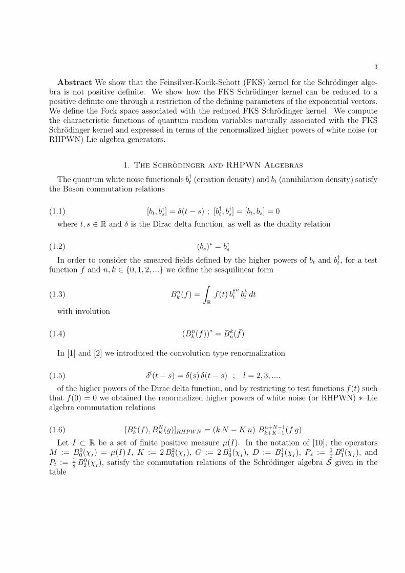
Abstract We show that the Feinsilver-Kocik-Schott (FKS) kernel for the Schrodinger alge-bra is not positive definite. We show how the FKS Schrodinger kernel can be reduced to apositive definite one through a restriction of the defining parameters of the exponential vectors.We define the Fock space associated with the reduced FKS Schrodinger kernel. We computethe characteristic functions of quantum random variables naturally associated with the FKSSchrodinger kernel and expressed in terms of the renormalized higher powers of white noise (orRHPWN) Lie algebra generators.

1. The Schrodinger and RHPWN Algebras

The quantum white noise functionals b†t (creation density) and bt (annihilation density) satisfythe Boson commutation relations

(1.1) [bt, b†s] = δ(t− s) ; [b†t , b

†s] = [bt, bs] = 0

where t, s ∈ R and δ is the Dirac delta function, as well as the duality relation

(1.2) (bs)∗ = b†s

In order to consider the smeared fields defined by the higher powers of bt and b†t , for a testfunction f and n, k ∈ {0, 1, 2, ...} we define the sesquilinear form

(1.3) Bnk (f) =

∫Rf(t) b†t

nbkt dt

with involution

(1.4) (Bnk (f))∗ = Bk

n(f)

In [1] and [2] we introduced the convolution type renormalization

(1.5) δl(t− s) = δ(s) δ(t− s) ; l = 2, 3, ....

of the higher powers of the Dirac delta function, and by restricting to test functions f(t) suchthat f(0) = 0 we obtained the renormalized higher powers of white noise (or RHPWN) ∗–Liealgebra commutation relations

(1.6) [Bnk (f), BN

K (g)]RHPWN = (k N −K n) Bn+N−1k+K−1 (f g)

Let I ⊂ R be a set of finite positive measure µ(I). In the notation of [10], the operatorsM := B0

0(χI) = µ(I) I, K := 2B2

0(χI), G := 2B1

0(χI), D := B1

1(χI), Px := 1

2B0

1(χI), and

Pt := 18B0

2(χI), satisfy the commutation relations of the Schrodinger algebra S given in the

table

4

(1.7)

M K G D Px PtM 0 0 0 0 0 0K 0 0 0 −2K −G −DG 0 0 0 −G −M −PxD 0 2K G 0 −Px −2PtPx 0 G M Px 0 0Pt 0 D Px 2Pt 0 0

The Feinsilver-Kocik-Schott (FKS) kernel (or Leibniz function), i.e. the inner product of theexponential vectors

(1.8) ψa,b(χI ) := eaB20(χ

I) ebB

10(χ

I) Φ = e

a2K e

b2G Φ

where a, b ∈ C with |a| < 2 and Φ is the Fock vacuum such that B02(χ

I) Φ = B0

1(χI) Φ = 0, is

given by (see Proposition 6.1 of [10] for c = µ(I) / 2 , m = µ(I) and a, b ∈ R ; a detailed proofcan be found in [11])

〈ψa,b(χI ), ψA,B(χI)〉 =

(1− a A

4

)−µ(I)2

eµ(I)

4

(a B2+4 b B+b2 A

4−a A

)(1.9)

= e−µ(I)

2ln (1− a A

4 ) eµ(I)

4

(a B2+4 b B+b2 A

4−a A

)

For a = A = 0 (1.9) reduces to the usual inner product of the Heisenberg algebra exponentialvectors, and for b = B = 0 it reduces to the inner product of the sl(2) (Square of White NoiseLie algebra) exponential vectors.

Using the commutativity of the Schrodinger algebra generators on disjoint sets, we mayextend the FKS kernel (1.9) to exponential vectors of the form

(1.10) Ψ(f, g) :=∏i

eaiB

20(χ

Ii)ebiB

10(χ

Ii)Φ = eB

20(f) eB

10(g) Φ

where f =∑

i ai χIi and g =∑

i bi χIi , with Ii ∩ Ij = � for i 6= j, are simple functions with|f | < 2 and we obtain

(1.11) 〈Ψ(f1, g1),Ψ(f2, g2)〉 = e− 1

2

∫ln(

1− f1 f24

)dµe

14

∫ ( f1 g22+4 g1 g2+g21 f24−f1 f2

)dµ

Proposition 1. The kernel (1.9) (and so also (1.11)) is not positive definite for arbitrary µ(I).This, in particular, implies the non-positive definiteness of the kernel of Proposition 6.1 of [10]for arbitrary c.

5

Proof. Denoting ‖ . . . ‖2 := 〈. . . , . . .〉, we examine the non–negativity of

Nk := ‖k∑i=1

ciψai,bi‖2

where k ∈ {1, 2, ...} and (for simplicity, as in [10]), ai, bi, ci ∈ R with |ai| < 2 for all i ∈{1, ..., k}.

For k = 1 we clearly have

N1 := |c1|2 ‖ψa1,b1‖2 = |c1|2 e−µ(I)

2ln

(1−a

214

)eµ(I)

4

(a1 b

21+4 b21+b21 a1

4−a21

)≥ 0

for all intervals I ⊂ R.

For k = 2 we have

N2 =2∑

i,j=1

ci cj e−µ(I)

2ln (1−

ai aj4 ) e

µ(I)4

(ai b

2j+4 bi bj+b2i aj

4−ai aj

)

= |c1|2 e−µ(I)

2ln

(1−a

214

)eµ(I)

4

(a1 b

21+4 b21+b21 a1

4−a21

)+ |c2|2 e

−µ(I)2

ln

(1−a

224

)eµ(I)

4

(a2 b

22+4 b22+b22 a2

4−a22

)

+ 2 c1 c2 e−µ(I)

2ln (1−a1 a2

4 ) eµ(I)

4

(a1 b

22+4 b1 b2+b21 a2

4−a1 a2

)

If c1 c2 ≥ 0 then, clearly, N2 ≥ 0. Suppose that c1 c2 < 0. The positive definiteness of N2

can be studied by checking the non-negativity of the determinants d1 and d2 of the principalminors of the real symmetric matrix

A2 =

e−µ(I)

2ln

(1−a

214

)eµ(I)

4

(a1 b

21+4 b21+b21 a1

4−a21

)e−

µ(I)2

ln (1−a1 a24 ) e

µ(I)4

(a1 b

22+4 b1 b2+b21 a2

4−a1 a2

)

e−µ(I)

2ln (1−a1 a2

4 ) eµ(I)

4

(a1 b

22+4 b1 b2+b21 a2

4−a1 a2

)e−µ(I)

2ln

(1−a

224

)eµ(I)

4

(a2 b

22+4 b22+b22 a2

4−a22

)

corresponding to N2. As in the case k = 1, we have

d1 = |c1|2 e−µ(I)

2ln

(1−a

214

)eµ(I)

4

(a1 b

21+4 b21+b21 a1

4−a21

)≥ 0

Moreover, since the case µ(I) = 0 is trivial, we may divide out µ(I) > 0 and proving d2 ≥ 0is equivalent to showing that

−1

2ln

(1− a2

1

4

)+

1

4

(a1 b

21 + 4 b2

1 + b21 a1

4− a21

)− 1

2ln

(1− a2

2

4

)+

1

4

(a2 b

22 + 4 b2

2 + b22 a2

4− a22

)

6

≥ − ln(

1− a1 a2

4

)+

1

2

(a1 b

22 + 4 b1 b2 + b2

1 a2

4− a1 a2

)which is equivalent to showing that

ln

(4− a1 a2√

(a21 − 4) (a2

2 − 4)

)≥ ((a2 − 2) b1 − (a1 − 2) b2)2

(a1 − 2) (a2 − 2) (a1 a2 − 2)

which is true since

((a2 − 2) b1 − (a1 − 2) b2)2

(a1 − 2) (a2 − 2) (a1 a2 − 2)≤ 0

and

4− a1 a2√(a2

1 − 4) (a22 − 4)

≥ 1⇔ 4 (a1 − a2)2 ≥ 0

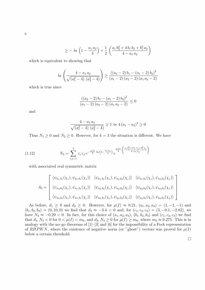
Thus N1 ≥ 0 and N2 ≥ 0. However, for k = 3 the situation is different. We have

N3 =3∑

i,j=1

ci cj e−µ(I)

2ln (1−

ai aj4 ) e

µ(I)4

(ai b

2j+4 bi bj+b2i aj

4−ai aj

)(1.12)

with associated real symmetric matrix

A3 =

〈ψa1,b1(χ

I), ψa1,b1(χ

I)〉 〈ψa1,b1(χ

I), ψa2,b2(χ

I)〉 〈ψa1,b1(χ

I), ψa3,b3(χ

I)〉

〈ψa2,b2(χI), ψa1,b1(χ

I)〉 〈ψa2,b2(χ

I), ψa2,b2(χ

I)〉 〈ψa2,b2(χ

I), ψa3,b3(χ

I)〉

〈ψa3,b3(χI), ψa1,b1(χ

I)〉 〈ψa3,b3(χ

I), ψa2,b2(χ

I)〉 〈ψa3,b3(χ

I), ψa3,b3(χ

I)〉

As before, d1 ≥ 0 and d2 ≥ 0. However, for µ(I) ≈ 0.21, (a1, a2, a3) = (1,−1,−1) and

(b1, b2, b3) = (0, 10, 0) we find that d3 ≈ −3.4 < 0 and, for (c1, c2, c3) = (3,−0.1,−2.82), wehave N3 ≈ −0.29 < 0. In fact, for this choice of (a1, a2, a3), (b1, b2, b3) and (c1, c2, c3) we findthat d3, N3 < 0 for 0 < µ(I) < m0, and d3, N3 ≥ 0 for µ(I) ≥ m0, where m0 ≈ 0.275. This is inanalogy with the no–go theorems of [1]–[3] and [6] for the impossibility of a Fock representationof RHPWN , where the existence of negative–norm (or ”ghost”) vectors was proved for µ(I)below a certain threshold.

�

7

2. Random variables associated with the Schrodinger algebra

For a fixed interval I, we will compute the vacuum characteristic function 〈Φ, ei sX Φ〉 of theself-adjoint operator

(2.1) X := xB20(χ

I) + x B0

2(χI) + y B1

0(χI) + y B0

1(χI)

where x, y ∈ C with x 6= 0.

For reasons explained in [3] we define the action of the RHPWN generators Bnk (f) on the

Fock vacuum vector Φ by

(2.2) Bnk (f) Φ :=

0 if n < k or n · k < 0

Bn−k0 (f) Φ if n > k ≥ 01

n+1

∫R f(t) dtΦ if n = k

Thus, in particular, B02(χ

I) Φ = B0

1(χI) Φ = 0 and B1

1(χI) Φ = µ(I) Φ.

Lemma 1. (i) If x, d, N and h satisfy the oscillator algebra commutation relations

(2.3) [d, x] = h ; [d, h] = [x, h] = 0 ; [N, x] = x ; [d,N ] = d

then for all analytic functions f and for all a ∈ C

(2.4) [N, f(x)] = x f ′(x) ; aN f(x) = f(a x) aN

Moreover, for all n,m ∈ N

(2.5) dn xm =n∧m∑j=0

(n,m

j

)xm−j dn−j hj

where

(2.6)

(n,m

j

)=

(n

j

)(m

j

)j!

(ii) If ∆, R and ρ satisfy the sl(2) algebra commutation relations

(2.7) [∆, R] = ρ ; [ρ,R] = 2R ; [∆, ρ] = 2 ∆

then

(2.8) et∆ eaR = eaR

1−a t (1− a t)−ρ et∆

1−a t

8

Proof. The proofs of (i) and (ii) can be found in [8].�

In the context of the RHPWN generators, in a manner consistent with the RHPWN repre-sentation of the Schrodinger algebra generators M,K,G,D, Px, Pt given in the previous section,

(2.9) R = K = 2B20(χ

I) ; ∆ = Pt =

1

8B0

2(χI) ; ρ = D = B1

1(χI)

and

(2.10) x = G = 2B10(χ

I) ; d = Px =

1

2B0

1(χI) ; N = D = B1

1(χI) ; h = M = B0

0(χI)

Lemma 2. For all a, b ∈ C

(i)

B02(χ

I) eaB

20(χ

I) = 4 a2B2

0(χI) eaB

20(χ

I) +(2.11)

4 a eaB20(χ

I) B1

1(χI) + eaB

20(χ

I) B0

2(χI)

(ii)

(2.12) B11(χ

I) ebB

10(χ

I) Φ =

(bB1

0(χI) +

µ(I)

2

)ebB

10(χ

I) Φ

(iii) For all n ≥ 0

(2.13) B02(χ

I) (B1

0(χI))n Φ = n (n− 1)µ(I) (B1

0(χI))n−2 Φ

(iv)

(2.14) B02(χ

I) ebB

10(χ

I) Φ = b2 µ(I) ebB

10(χ

I) Φ

(v) For all n ≥ 0

(2.15) B01(χ

I) (B2

0(χI))n = 2nB1

0(χI) (B2

0(χI))n−1 + (B2

0(χI))nB0

1(χI)

(vi)

(2.16) B01(χ

I) eaB

20(χ

I) = 2 aB1

0(χI) eaB

20(χ

I) + eaB

20(χ

I) B0

1(χI)

9

Proof. (i) By (2.9) and lemma 1(ii)

B02(χ

I) eaB

20(χ

I) =

∂

∂ t|t=0

(etB

02(χ

I) eaB

20(χ

I))

=∂

∂ t|t=0

(e

a1−4 t a

B20(χ

I) (1− 4 t a)−B

11(χ

I) e

t1−4 t a

B02(χ

I))

= 4 a eaB20(χ

I) B1

1(χI) + eaB

20(χ

I) B0

2(χI)

(ii) By (2.10), (2.2) and lemma 1(i)

B11(χ

I) ebB

10(χ

I) Φ =

([B1

1(χI), ebB

10(χ

I)] + ebB

10(χ

I) B1

1(χI))

Φ

=

(bB1

0(χI) +

µ(I)

2

)ebB

10(χ

I) Φ

(iii) For n = 0, both sides of (2.13) are zero. For n = 1, since

B02(χ

I)B1

0(χI) = 2B0

1(χI) +B1

0(χI)B0

2(χI)

again both sides of (2.13) are zero. For n ≥ 2 we have

an := B02(χ

I) (B1

0(χI))n Φ

= B02(χ

I)B1

0(χI) (B1

0(χI))n−1 Φ

= (2B01(χ

I) +B1

0(χI)B0

2(χI)) (B1

0(χI))n−1 Φ

= 2B01(χ

I) (B1

0(χI))n−1 Φ +B1

0(χI) an−1

By (2.5)

B01(χ

I) (B1

0(χI))n−1 = (n− 1) (B1

0(χI))n−2B0

0(χI) + (B1

0(χI))n−1B0

1(χI)

Thus

10

an = 2µ(I) (n− 1) (B10(χ

I))n−2 Φ +B1

0(χI) an−1

= 2µ(I) ((n− 1) + (n− 2)) (B10(χ

I))n−2 Φ + (B1

0(χI))2 an−2

= 2µ(I) ((n− 1) + (n− 2) + (n− 3)) (B10(χ

I))n−2 Φ + (B1

0(χI))3 an−3

= ...

= 2µ(I) ((n− 1) + (n− 2) + (n− 3) + ...+ (n− (n− 1))) (B10(χ

I))n−2 Φ + (B1

0(χI))n−1 a1

= 2µ(I) ((n− 1) + (n− 2) + (n− 3) + ...+ (n− (n− 1))) (B10(χ

I))n−2 Φ

= 2µ(I) (n (n− 1)− (1 + 2 + ...+ (n− 1)) (B10(χ

I))n−2 Φ

= 2µ(I)

(n (n− 1)− n (n− 1)

2

)(B1

0(χI))n−2 Φ

= µ(I)n (n− 1) (B10(χ

I))n−2 Φ

(iv) Using (iii)

B02(χ

I) ebB

10(χ

I) Φ = B0

2(χI)∞∑n=0

bn

n!(B1

0(χI))n

Φ

=∞∑n=0

bn

n!B0

2(χI) (B1

0(χI))n

Φ

=∞∑n=0

bn

n!n (n− 1)µ(I) (B1

0(χI))n−2 Φ

=∞∑n=2

bn

n!n (n− 1)µ(I) (B1

0(χI))n−2 Φ

= b2 µ(I)∞∑n=2

bn−2

(n− 2)!(B1

0(χI))n−2 Φ

= b2 µ(I) ebB10(χ

I) Φ

(v) As in the proof of (iii)

11

bn := B01(χ

I) (B2

0(χI))n

= B01(χ

I)B2

0(χI) (B2

0(χI))n−1

= (2B10(χ

I) +B2

0(χI)B0

1(χI)) (B2

0(χI))n−1

= 2B10(χ

I) (B2

0(χI))n−1 +B2

0(χI) bn−1

= 4B10(χ

I) (B2

0(χI))n−1 + (B2

0(χI))2 bn−2

= ...

= 2nB10(χ

I) (B2

0(χI))n−1 + (B2

0(χI))n b0

= 2nB10(χ

I) (B2

0(χI))n−1 + (B2

0(χI))nB0

1(χI)

(vi)

B01(χ

I) eaB

20(χ

I) = B0

1(χI)∞∑n=0

an

n!(B2

0(χI))n

=∞∑n=0

an

n!B0

1(χI) (B2

0(χI))n

=∞∑n=0

an

n!(2nB1

0(χI) (B2

0(χI))n−1 + (B2

0(χI))nB0

1(χI))

= 2 aB10(χ

I)∞∑n=0

an−1

(n− 1)!(B2

0(χI))n−1

+∞∑n=0

an

n!(B2

0(χI))nB0

1(χI)

= 2 aB10(χ

I) eaB

20(χ

I) + eaB

20(χ

I)B0

1(χI)

�

Lemma 3. For all s ∈ R

ei sX Φ = ew1(s)B20(χ

I) ew2(s)B1

0(χI

) ew3(s) Φ

where X is as in (2.1) and

w1(s) =i

2

√x

xtanh (2 s |x|)(2.17)

w2(s) =i

2

y

x(1− sech (2 s |x|)) +

y

2 |x|tanh(2 s |x|)(2.18)

and

12

(2.19)

w3(s) =

(|y|2 + i s (y2 x+ x y2)

4 |x|2− i (y2 x+ x y2)

8 |x|3tanh (2 s |x|)− |y|

2

4 |x|2sech (2 s |x|)

)µ(I)

Proof. We will show that w1(s), w2(s) and w3(s) satisfy the differential equations

w′1(s) = 4 i x w1(s)2 + i x ; w1(0) = 0 (Riccati ODE)(2.20)

w′2(s) = 4 i x w1(s)w2(s) + 2 y w1(s) + y ; w2(0) = 0 (Linear ODE)(2.21)

w′3(s) = (i x w2(s)2 + y w2(s) + 2 i x w1(s))µ(I) ; w3(0) = 0(2.22)

whose solutions are given by (2.17), (2.18) and (2.19) respectively.

In so doing, let

(2.23) E Φ := es(xB20(χ

I)+x B0

2(χI

)+y B10(χ

I)+y B0

1(χI

)) Φ

and also

(2.24) E Φ := ew1(s)B20(χ

I) ew2(s)B1

0(χI

) ew3(s) Φ

where wi(0) = 0 for i ∈ {1, 2, 3}. Then, (2.24) implies that

(2.25)∂

∂ sE Φ =

(w′1(s)B2

0(χI) + w′2(s)B1

0(χI) + w′3(s)

)E Φ

and, since by lemma 2,

B02(χ

I)E Φ = (4w1(s)2B2

0(χI) + 4w1(s)w2(s)B1

0(χI)(2.26)

+(2w1(s) + w2(s)2)µ(I))E Φ

and

B01(χ

I)E Φ =

(2w1(s)B1

0(χI) + µ(I)w2(s)

)E Φ(2.27)

from (2.23) we also obtain

∂

∂ sE Φ = ((4 i x w1(s)2 + i x)B2

0(χI) + (4 i x w1(s)w2(s) + 2 y w1(s) + y)B1

0(χI)(2.28)

+(i x w2(s)2 + y w2(s) + 2 i x w1(s))µ(I))E Φ

From (2.25) and (2.28), by equating coefficients of B20(χ

I), B1

0(χI) and 1, we obtain (2.17),

(2.18) and (2.19) thus completing the proof.�

13

Proposition 2. (Characteristic Function) For all s ∈ R

〈Φ, ei sX Φ〉 =(2.29)

e

(|y|2+i s(y2 x+x y2)

4 |x|2−i(y2 x+x y2)

8 |x|3tanh (2 s |x|)− |y|

2

4 |x|2sech (2 s |x|)

)µ(I)

Proof. Using lemma 2 and the fact that for any z ∈ C

(2.30) ez B02(χ

I) Φ = ez B

01(χ

I) Φ = Φ

we have

〈Φ, ei sX Φ〉 = 〈Φ, ew1(s)B20(χ

I) ew2(s)B1

0(χI

) ew3(s) Φ〉(2.31)

= 〈ew2(s)B01(χ

I) ew1(s)B0

2(χI

) Φ, ew3(s) Φ〉= 〈Φ, ew3(s) Φ〉= ew3(s) 〈Φ,Φ〉= ew3(s)

= e

(|y|2+i s(y2 x+x y2)

4 |x|2−i(y2 x+x y2)

8 |x|3tanh (2 s |x|)− |y|

2

4 |x|2sech (2 s |x|)

)µ(I)

�

3. Positive definite restrictions of the Schrodinger kernel

To overcome the problem of the non-positive definiteness of the FKS kernel (1.9) we lookfor a restriction of the parameters a, b ∈ C, |a| < 2, in the definition (1.8) of the exponentialvectors ψa,b(χI ). We notice that if a, b, A,B ∈ C are such that

(3.1) a B2 + b2A = 0

i.e. if (a, b), (A,B) ∈ Sλ where, for given λ ∈ R,

(3.2) Sλ := {(a, b) ∈ C2 / a = i λ b2, |λ| |b|2 < 2}then the FKS kernel (1.9) reduces to

〈ψa,b(χI ), ψA,B(χI)〉 =

(1− a A

4

)−µ(I)2

eµ(I)

4b B

1− a A4(3.3)

=

(1− a A

4

)−µ(I)2

eµ(I)

4 (b B)∑∞n=0 ( a A4 )

n

14

The kernels Ki : C2 × C2 → C defined for i ∈ {1, 2, 3} by

K1((a, b), (A,B)) :=

(1− a A

4

)−µ(I)2

(3.4)

K2((a, b), (A,B)) :=µ(I)

4b B(3.5)

K3((a, b), (A,B)) := limρ→∞

K3,ρ((a, b), (A,B))(3.6)

where, for ρ ≥ 1,

(3.7) K3,ρ((a, b), (A,B)) :=

ρ∑n=0

(a A

4

)nare positive definite, since K1 is the well-known sl(2) kernel, K2 and K3,ρ are Heisenberg-type

kernels and K3 is a limit of positive definite kernels . Therefore K1 eK2K3 , i.e. (3.3), is also a

positive definite kernel.

For given λ ∈ R and I ⊂ R we introduce the notation

ψ(b) := ψi λ b2,b(χI ) = ei λ b2B2

0(χI

) ebB10(χ

I) Φ(3.8)

〈ψ(b), ψ(B)〉λ := 〈ψi λ b2,b(χI ), ψi λB2,B(χI)〉 =

(1− λ2

4(b B)2

)−µ(I)2

eb B

4−λ2 (b B)2µ(I)

(3.9)

and its extension to simple functions f =∑

j bj χIj

Ψ(f) := Ψi λ f2,f =∏j

ei λ b2j B

20(χ

Ij)ebj B

10(χ

Ij)Φ = ei λB

20(f2) eB

10(f) Φ(3.10)

〈Ψ(f),Ψ(g)〉λ := 〈Ψ(i λ f 2, f),Ψ(i λ g2, g)〉 = e− 1

2

∫ln

(1−λ

2 (f g)2

4

)dµe∫ f g

4−λ2 (f g)2dµ

(3.11)

If f = b χI then Ψ(f) = ψ(b).

For λ ∈ R we define the (restricted) Schrodinger Fock space FS(λ) as the closure of thelinear span of the exponential vectors Ψ(f) defined in (3.10) with respect to the inner product〈Ψ(f),Ψ(g)〉λ defined in (3.11).

The study of FS(λ) and the random variables that can be defined on it, is in progress.

15

References

[1] Accardi, L., Boukas, A.: Renormalized higher powers of white noise (RHPWN) and conformal field theory,Infinite Dimensional Analysis, Quantum Probability, and Related Topics 9, No. 3, (2006) 353-360.

[2] Accardi, L., Boukas, A.: The emergence of the Virasoro and w∞ Lie algebras through the renormalizedhigher powers of quantum white noise , International Journal of Mathematics and Computer Science, 1,No.3, (2006) 315–342.

[3] Accardi, L., Boukas, A.: Fock representation of the renormalized higher powers of white noise and theVirasoro–Zamolodchikov–w∞ ∗–Lie algebra, J. Phys. A: Math. Theor., 41 (2008).

[4] Accardi, L., Boukas, A.: Cohomology of the Virasoro–Zamolodchikov and Renormalized Higher Powers ofWhite Noise ∗–Lie algebras, Infinite Dimensional Anal. Quantum Probab. Related Topics, Vol. 12, No. 2(2009) 120.

[5] Accardi, L., Boukas, A.: Quantum probability, renormalization and infinite dimensional ∗–Lie algebras,SIGMA (Symmetry, Integrability and Geometry: Methods and Applications), 5 (2009), 056, 31 pages.

[6] Accardi, L., Boukas, A., Franz, U.: Renormalized powers of quantum white noise, Infinite DimensionalAnalysis, Quantum Probability, and Related Topics, (1) (2006) 129–147.

[7] Accardi L., Lu Y. G., Volovich I. V.: White noise approach to classical and quantum stochastic calculi,Lecture Notes of the Volterra International School of the same title, Trento, Italy (1999), Volterra Centerpreprint 375, Universita di Roma Torvergata.

[8] Feinsilver, P. J., Schott, R.: Algebraic structures and operator calculus. Volumes I and III, Kluwer, 1993.[9] Feinsilver, P. J., Schott, R.: Differential relations and recurrence formulas for representations of Lie groups,

Stud. Appl. Math., 96 (1996), no. 4, 387–406.[10] Feinsilver, P. J., Kocik, J., Schott, R.: Representations of the Schroedinger algebra and Appell systems,

Fortschr. Phys. 52 (2004), no. 4, 343–359.[11] Feinsilver, P. J., Kocik, J., Schott, R.: Berezin quantization of the Schrodinger algebra, Infinite Dimensional

Analysis, Quantum Probability, and Related Topics, Vol. 6, No. 1 (2003), 57–71.