Regularized Positive-Definite Fourth Order Tensor FieldEstimation from DW-MRI★

Angelos Barmpoutis, Baba C. Vemuri, Dena Howland, and John R. ForderUniversity of Florida, Gainesville FL 32611, USAAngelos Barmpoutis: abarmpou@cise.ufl.edu; Baba C. Vemuri: vemuri@cise.ufl.edu; Dena Howland:howland@mbi.ufl.edu; John R. Forder: jforder@mbi.ufl.edu

AbstractIn Diffusion Weighted Magnetic Resonance Image (DW-MRI) processing, a 2nd order tensor hasbeen commonly used to approximate the diffusivity function at each lattice point of the DW-MRIdata. From this tensor approximation, one can compute useful scalar quantities (e.g. anisotropy, meandiffusivity) which have been clinically used for monitoring encephalopathy, sclerosis, ischemia andother brain disorders. It is now well known that this 2nd-order tensor approximation fails to capturecomplex local tissue structures, e.g. crossing fibers, and as a result, the scalar quantities derived fromthese tensors are grossly inaccurate at such locations. In this paper we employ a 4th order symmetricpositive-definite (SPD) tensor approximation to represent the diffusivity function and present a noveltechnique to estimate these tensors from the DW-MRI data guaranteeing the SPD property. Severalarticles have been reported in literature on higher order tensor approximations of the diffusivityfunction but none of them guarantee the positivity of the estimates, which is a fundamental constraintsince negative values of the diffusivity are not meaningful. In this paper we represent the 4th-ordertensors as ternary quartics and then apply Hilbert’s theorem on ternary quartics along with theIwasawa parametrization to guarantee an SPD 4th-order tensor approximation from the DW-MRIdata. The performance of this model is depicted on synthetic data as well as real DW-MRIs from aset of excised control and injured rat spinal cords, showing accurate estimation of scalar quantitiessuch as generalized anisotropy and trace as well as fiber orientations.

1 IntroductionAdvances in medical imaging during the last decade have made it possible to collect massiveamounts of data, which can be used to analyze the underlying connectivity of the tissues beingscanned. More specifically, acquisition of magnetic resonance image (MRI) data that measuresthe apparent diffusivity of water in tissue in vivo has been extensively used for computing thediffusivity at each image lattice point.

A 2nd order tensor has commonly been used to approximate the diffusivity function from agiven set of, usually seven or more, acquired DW-MR images [5]. The approximated diffusivityfunction is given by

★This research was in part funded by the NIH grant EB007082 to BCV, and in part by the University of Florida Alumni Fellowship toAB.Corresponding author: Baba C Vemuri.Publisher's Disclaimer: This is a PDF file of an unedited manuscript that has been accepted for publication. As a service to our customerswe are providing this early version of the manuscript. The manuscript will undergo copyediting, typesetting, and review of the resultingproof before it is published in its final citable form. Please note that during the production process errors may be discovered which couldaffect the content, and all legal disclaimers that apply to the journal pertain.

NIH Public AccessAuthor ManuscriptNeuroimage. Author manuscript; available in PMC 2010 March 1.

Published in final edited form as:Neuroimage. 2009 March ; 45(1 Suppl): S153–S162. doi:10.1016/j.neuroimage.2008.10.056.

NIH

-PA Author Manuscript

NIH

-PA Author Manuscript

NIH

-PA Author Manuscript

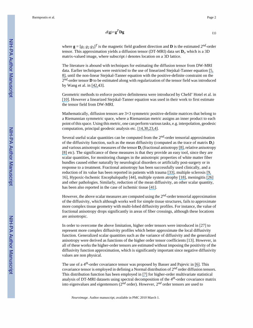
(1)

where g = [g1 g2 g3]T is the magnetic field gradient direction and D is the estimated 2nd-ordertensor. This approximation yields a diffusion tensor (DT-MRI) data set Di, which is a 3Dmatrix-valued image, where subscript i denotes location on a 3D lattice.

The literature is abound with techniques for estimating the diffusion tensor from DW-MRIdata. Earlier techniques were restricted to the use of linearized Stejskal-Tanner equation [5,8], until the non-linear Stejskal-Tanner equation with the positive-definite constraint on the2nd-order tensor D to be estimated along with regularization of the tensor field was introducedby Wang et al. in [42,43].

Geometric methods to enforce positive definiteness were introduced by Chefd’ Hotel et al. in[10]. However a linearized Stejskal-Tanner equation was used in their work to first estimatethe tensor field from DW-MRI.

Mathematically, diffusion tensors are 3×3 symmetric positive-definite matrices that belong toa Riemannian symmetric space, where a Riemannian metric assigns an inner product to eachpoint of this space. Using this metric, one can perform various tasks, e.g. interpolation, geodesiccomputation, principal geodesic analysis etc. [14,30,23,4].

Several useful scalar quantities can be computed from the 2nd-order tensorial approximationof the diffusivity function, such as the mean diffusivity (computed as the trace of matrix Di)and various anisotropic measures of the tensor Di (fractional anisotropy [8], relative anisotropy[8] etc). The significance of these measures is that they provide an easy tool, since they arescalar quantities, for monitoring changes in the anisotropic properties of white matter fiberbundles caused either naturally by neurological disorders or artificially post-surgery or inresponse to a treatment. Fractional anisotropy has been successfully used clinically, and areduction of its value has been reported in patients with trauma [33], multiple sclerosis [9,16], Hypoxic-Ischemic Encephalopathy [44], multiple system atrophy [18], meningitis [26]and other pathologies. Similarly, reduction of the mean diffusivity, an other scalar quantity,has been also reported in the case of ischemic tissue [41].

However, the above scalar measures are computed using the 2nd-order tensorial approximationof the diffusivity, which although works well for simple tissue structures, fails to approximatemore complex tissue geometry with multi-lobed diffusivity profiles. For instance, the value offractional anisotropy drops significantly in areas of fiber crossings, although these locationsare anisotropic.

In order to overcome the above limitation, higher order tensors were introduced in [27] torepresent more complex diffusivity profiles which better approximate the local diffusivityfunction. Generalized scalar quantities such as the variance of diffusivity and the generalizedanisotropy were derived as functions of the higher order tensor coefficients [13]. However, inall of these works the higher-order tensors are estimated without imposing the positivity of thediffusivity function approximation, which is significantly important since negative diffusivityvalues are non physical.

The use of a 4th-order covariance tensor was proposed by Basser and Pajevic in [6]. Thiscovariance tensor is employed in defining a Normal distribution of 2nd order diffusion tensors.This distribution function has been employed in [7] for higher-order multivariate statisticalanalysis of DT-MRI datasets using spectral decomposition of the 4th-order covariance matrixinto eigenvalues and eigentensors (2nd order). However, 2nd order tensors are used to

Barmpoutis et al. Page 2

Neuroimage. Author manuscript; available in PMC 2010 March 1.

NIH

-PA Author Manuscript

NIH

-PA Author Manuscript

NIH

-PA Author Manuscript

approximate the diffusivity of each lattice point of a MR data set, failing to capture complexlocal tissue geometries, such as fiber crossings.

In [25], Moakher and Norris presented a way to minimize the distance between a given higher-order tensor and the closest elasticity tensor of higher symmetry, using different metrics. Thiswork was recently extended by Moakher [24] where in he developed an interesting frameworkto describe the geometry of 4th-order tensors. A 4th-order symmetric positive definite tensorin three dimensions is represented by a 2nd-order symmetric positive definite tensor in sixdimensions and therefore, one can use the Riemannian metric of the space of 6×6 SPD matricesfor the SPD 4th-order tensor computations. However, this framework fails to parameterize thefull space of SPD 4th-order tensors. For example the groups of SPD tensors

and , where a, b, c are positive valued coefficients,can not be written in the form of 6×6 SPD matrices. Furthermore, the Riemannian metric ofsymmetric positive-definite 2nd-order tensors in six dimensions assigns infinite distancebetween 6×6 SPD and 6 × 6 semi-definite matrices. The SPD tensors in the aforementionedexamples correspond to 6 × 6 semi-definite matrices and therefore, the Riemannian metricassigns infinite distance between them although their corresponding coefficients can bearbitrarily close. This leads to arbitrarily large errors in tensor processing and one shouldtherefore strive to seek a more appropriate framework to characterize the full space ofsymmetric positive definite 4th-order tensors.

The first reported method in literature to impose the positivity constraint on 4th-order diffusiontensors was presented in Barmpoutis et al. [1] and in their work, they parameterize the fullspace of positive definite 4th-order tensors. They represent the 4th-order tensor as ahomogeneous polynomial of degree 4 in 3 variables, the so called ternary quartic. They theninvoke Hilbert’s theorem on ternary quartics [17] according to which, any non-negative 4th-order tensor can be expressed as a sum of squares of three quadratic (2nd-order) forms, whichcan be further expressed as an equivalent semi-definite 2nd-order tensor using a CCT

parametrization, where C is a 6 × 3 coefficient matrix. Although by using this parametrizationthe whole space of SPD 4th-order tensors is covered, the elements on the boundary of this spaceare also included i.e. the positive semi-definite 4th-order tensors. Furthermore, the space ofparameters is not unique since the coefficients C and their antipodal symmetric −Cparameterize the same tensor. This non-uniqueness issue leads to problems when regularizingthe field of coefficients C thus motivating us to seek a new way for parameterizing andestimating regularized 4th-order tensors fields.

In this paper we propose a novel parametrization of the 4th-order tensors for imposing thepositivity of the estimated diffusivity. In this parametrization we express the 6 × 6 matrix G =CCT using its Iwasawa coordinates [36]. By combining the Iwasawa formulation with theHilbert’s theorem on ternary quartics [17], we are interested in estimating Iwasawadecomposable 6×6 symmetric positive semi-definite matrices of at most rank-3. We deriveformulas for uniquely computing the tensor coefficients as functions of the parameters of ourmodel. The unknown parameters are estimated from a given DW-MRI data set by minimizingan energy function in which we add a regularization term for estimating smooth 4th-order tensorfields.

The key contribution of this work is the use of a parametrization which can decompose any 6× 6 symmetric positive semi-definite matrix of at most rank-3. This parametrization has twomain advantages: a) it minimizes the solution space by overcoming the non-uniquenessproblems of the model in [1] and b) allows the simultaneous estimation and regularization ofthe 4th-order tensor field. The motivation for using an estimated positive higher-order tensormodel is that one can derive the generalized higher-order extensions of the commonly used2nd-order scalar measures for monitoring various brain diseases. In our experimental results

Barmpoutis et al. Page 3

Neuroimage. Author manuscript; available in PMC 2010 March 1.

NIH

-PA Author Manuscript

NIH

-PA Author Manuscript

NIH

-PA Author Manuscript

we show that such scalar measures can be more accurately estimated by using the proposedframework compared to other methods. We show that our model is robust to noise in estimatingfiber orientations as well as scalar measures derived from the 4th-order tensor coefficients suchas the generalized trace [13]. This demonstrates that the proposed framework is a directlyapplicable tool that extends efficiently the clinically used measures by overcoming thelimitations of the current models in literature.

The rest of the paper is organized as follows: In section 2, we present a novel parametrizationof the 4th-order tensors that is used to enforce the positivity of the estimated tensors using theIwasawa decomposition of the Gram matrix. In section 2.1, we present a functionalminimization method to estimate 4th-order tensors from diffusion-weighted MR images.Furthermore, in section 2.2 we propose a distance measure for the space of 4th-order tensors,and employ it for estimating a smoothly varying tensor field as well as estimating thegeneralized variance of the tensors. Section 3 contains the experimental results andcomparisons with other methods using simulated diffusion MRI data and real MR database ofexcised rat spinal cords. In section 4 we conclude.

2 Diffusion tensors of 4th orderThe diffusivity function has been commonly modeled in literature by Eq. (1) using a 2nd-ordertensor. Studies have shown that this approximation fails to model complex local structures ofthe diffusivity in real tissues [28] and higher-order tensors or other methods for multi-fiberapproximation must instead be employed [40,27,11,39,38,37,22,21]. In the case of 4th-ordertensors, the diffusivity function can be expressed using the standard notation of quartic forms[31] as

(2)

where g = [g1 g2 g3]T is the magnetic field gradient direction. It should be noted that in thecase of 4th-order symmetric tensors there are 15 unique coefficients Di,j,k, while in the case of2nd-order tensors we only have 6.

In DW-MRI the diffusivity of the water is a positive quantity. This property is essential sincenegative diffusion coefficients are non-physical. However, in the parametrization of Eq. 2 thereis no guarantee that the estimated coefficients Di,j,k form a positive tensor. Therefore, there isneed for the development of a new parametrization of the 4th-order tensor, which guaranteesthe positivity of the estimated tensor.

Letting g1, g2 and g3 in (2) be the variables, the equivalence between symmetric tensors andhomogeneous polynomials is straightforward to establish. Moreover, if a symmetric tensor ispositive, then its corresponding polynomial must be positive for all real-valued variables.Hence, here we are concerned with the positive definiteness of homogenous polynomials ofdegree 4 in 3 variables, or the so called ternary quartics. Hilbert in 1888 proved the followingtheorem on ternary quartics (see [34,32] for a modern exposition) that we will employ in thiswork:

Theorem 1

There exists an identity in which d is a real ternary form d = d(g1, g2, g3) of degreefour which is positive semi-definite and the pi are quadratic forms with real coefficients.

Barmpoutis et al. Page 4

Neuroimage. Author manuscript; available in PMC 2010 March 1.

NIH

-PA Author Manuscript

NIH

-PA Author Manuscript

NIH

-PA Author Manuscript

By using this theorem, Eq. (2) can be expressed as a sum of 3 squares of quadratic forms as

(3)

where, v is a properly chosen vector of monomials, (e.g. ), C = [c1|c2|c3] is a 6 × N matrix by stacking the 6 coefficient vectors ci and G = CCT is the so calledGram matrix.

The Gram matrix G in Eq. 3 is positive semi-definite and has at most rank 3. Here we shouldemphasize that G being semi-definite does not imply that the 4th-order tensor d is also semi-definite, since the vector space of the former is 6-dimensional (i.e. vectors v) while thecorresponding vector space of the latter is 3-dimensional (i.e. vectors g). In fact, using theparametrization of Eq. 3 the whole space of the strictly positive definite ternary quartics aswell as those which are semi-definite is spanned.

Given a Gram matrix, the CCT parametrization in Eq. 3 is not unique, i.e. there exist differentmatrices C which parameterize the same Gram matrix. For example C parameterizes the sameGram matrix as its antipodal pair −C. Furthermore, there are infinitely many orthogonalmatrices that yield the same G when appropriately applied in the aforementionedparametrization. This is due to the orthogonality property (OOT = I) of the rotation matricesO, where I is the identity matrix. Thus, in the case that C is of size 6×3, for any 3×3 orthogonalmatrix O we have (CO)(CO)T = CCT. This produces an infinite solution space, whichtheoretically can not be handled by the optimization techniques. We should also note that inEq. 3 there are in total 18 parameters in C, which are 3 more coefficients than the number ofunique tensor coefficients in Eq. 2. The non uniqueness issues of the Gram matrix were alsodiscussed by Powers et al. in [31], investigating how many fundamentally differnent Grammatrices parametrize the same ternary quartic.

In order to overcome the above issues, we use the Iwasawa decomposition which representsthe components of a positive definite or semi-definite matrix in the Iwasawa coordinates [19,20]. Every n × n positive definite matrix G can be uniquely expressed using its Iwasawacomponents as follows.

(4)

where W and V are SPD matrices of size k×k and m×m respectively, X ∈ ℜk×m and A[B]denotes BTAB.

In the case of n × n positive semi-definite matrices of at most rank-k, the Iwasawa coordinatesare also given by Eq. 4 by setting rank(W) + rank(V) ≤ k. By computing the matrixmultiplications in Eq. 4 we derive the following parametrization of positive semi-definitematrices

(5)

Barmpoutis et al. Page 5

Neuroimage. Author manuscript; available in PMC 2010 March 1.

NIH

-PA Author Manuscript

NIH

-PA Author Manuscript

NIH

-PA Author Manuscript

where W and V are 3×3 positive definite or positive semi-definite matrices and their ranks sumup to k. Furthermore, by using the Cholesky decomposition of W = AAT, where A is a lowertriangular matrix with non-negative diagonal elements, we can establish equivalence betweenthe parametrization in Eq. 5 and that in Eq. 3 by defining B to be the matrix that satisfies theequation BAT = XT W. By using the above we derive the following parametrization for theGram matrix

(6)

where and B ∈ ℜ3×3.

If W is positive definite, then the Cholesky factor A is unique, B = XT A is also unique, V =0 and therefore, the parametrization in Eq. 6 is unique. Note that in Eq. 6 there are in total 15parameters, 6 in A and 9 in B, which is equal to the number of unique tensor coefficients inEq. 2.

According to Theorem 1, Eq. 6 spans the whole space of positive semi-definite ternary quarticsbut can be used to define a parametrization for the case of strictly positive definite 4th-orderternary quartics as follows:

Lemma 1For every real positive definite ternary quartic d there exists an arbitrarily small positive realnumber c such that d can be written as the sum of the ternary quartic c(x2 + y2 + z2)2 and threesquares of quadratic forms.

ProofLet d(g) be a strictly positive definite ternary quartic. Therefore, d(g) > 0 ∀g ∈ S2, where,S2 is the unit sphere, i.e. the space of unit vectors g. We define the following ternary quartic

, where c is any real number in the interval 0 < c ≤ ming∈S2d(g). Since c > 0 this

ternary quartic is also positive definite. Let us now define . Sinceming∈S2f(g) = ming∈S2d(g) − c ≥ 0, f(g) is a positive semi-definite ternary quartic and thereforecan be expressed as a sum of three squares of quadratic forms (by Theorem 1). Thus, every

positive definite ternary quartic d(g) can be written as where c is anarbitrarily small positive real number, which proves the lemma.

The corresponding diffusivity function can be expressed using the Iwasawa coordinates asfollows:

(7)

Barmpoutis et al. Page 6

Neuroimage. Author manuscript; available in PMC 2010 March 1.

NIH

-PA Author Manuscript

NIH

-PA Author Manuscript

NIH

-PA Author Manuscript

where C is a 3 × 3 matrix whose elements equal to the same arbitrarily small positive real

number c, v is a properly chosen vector of monomials, (e.g. ), W, Vand X are defined as in Eq. 5, and A and B are defined as in Eq. 6.

Here we should note that in practice due to finite precision computations c can be set to thesmallest possible value of a finite precision machine and therefore, is considered as a knownvariable. In the double-precision floating-point IEEE 754-1985 standard the smallest positivevalue is approximately c =10−308.

Furthermore, we should emphasize that the semi-definite property of G does not necessarilyimply semi-definiteness of d(g) since the former is semi-definite in ℜ6 while the latter may besemi-definite in ℜ3. In particular, using the proposed parametrization (Eq. 7), we computesemi-definite matrices G that correspond to strictly positive-definite d(g).

Given a Gram matrix, which in our case is parameterized using the matrices A and B in Eq. 7,we can uniquely compute the tensor coefficients Di,j,k by using the formulas in table 1. In theseformulas the tensor coefficients are expressed as functions of the components of A, B and thefixed parameter c.

Therefore, we can employ the parametrization in Eq. 7 for the estimation of the coefficientsDi,j,k of the diffusion tensor from MR images using the following two steps: 1) first estimatethe A and B matrices from the given images by using a functional minimization method(minimization of Eq. 8 using the Lavenberg-Marquardt nonlinear least-squares method), andthen 2) compute the unique coefficients Di,j,k of the 4th-order tensor by using formulas in table1.

In the following section we will employ this method to enforce the positive definite propertyof the estimated fourth order diffusion tensors from the diffusion weighted MR images.

2.1 Estimation from DWIThe coefficients Di,j,k of a 4th order diffusion tensor can be estimated from diffusion-weightedMR images by minimizing the following cost function:

(8)

where G is the Iwasawa parameterized Gram matrix given by Eq. 7, M is the number of thediffusion weighted images associated with gradient vectors gi and b-values bi; Si is thecorresponding acquired signal and S0 is the zero gradient signal. Using the magnetic fieldgradient directions gi we construct the 6-dimensional vectors

. In Eq. (8), the 4th order diffusion tensor is parameterizedusing the 3 × 3 matrices A and B which form together the Gram matrix G. Having estimatedthe matrices A and B that minimize Eq. (8), the coefficients Di,j,k can be computed directlyusing the formulas in Table 1. S0 can either be assumed to be known or estimatedsimultaneously with the coefficients Di,j,k by minimizing Eq. (8).

In the implementation of the proposed method, in order to enforce the diagonal elements a1,1,a2,2 and a3,3 of matrix A to be non negative, we should use a mapping of ℜ to the space ofnon-negative real numbers. In order for this mapping to be unique (one to one), the target spacemust be open, hence we seek a mapping to the positive part of ℜ. This does not limit the solutionspace in our implementation, since it has been shown that in finite precision arithmetic, open

Barmpoutis et al. Page 7

Neuroimage. Author manuscript; available in PMC 2010 March 1.

NIH

-PA Author Manuscript

NIH

-PA Author Manuscript

NIH

-PA Author Manuscript

spaces are equivalent to closed spaces (Wang et al. [43]). In our experiments we used theexponential mapping and and therefore, in theminimization we solve for and instead of a1,1, a2,2 and a3,3. The total number ofunknown parameters in G in Eq. 8 are 15 and they are the following: , a2,1, a3,1,a3,2 and the 9 elements of matrix B.

Starting with an initial guess for S0, A and B we can use any gradient based optimization methodin order to minimize Eq. (8). We should note here that the exponent in Eq. (8) is in the formof a polynomial and therefore its gradient with respect to the unknown coefficients is easilyderived analytically.

Given A and B at each iteration of the optimization algorithm we can update S0 by againminimizing Eq. (8). The derivative of this equation with respect to the unknown S0 is

(9)

By setting Eq. (9) equal to zero, we derive the following update formula for S0

(10)

In our experiments we used the well known Lavenberg-Marquardt (LM) nonlinear least-squares method, which has advantages over other optimization methods, in terms of stabilityand computational burden. The average execution time of our implementation on an AMDAthlon 2GHz was N ×M ×0.000545 seconds where N is the number of voxels per image andM is the number of the acquired DW-MR images used in the estimation of the 4th-order tensorfield.

2.2 Distance measureIn the previous section we discussed how to estimate the positive-definite 4th-order tensorsfrom DW-MRI data by minimizing Eq. 8. The 4th-order tensors are by definition (Eq. 2)smoothly varying functions (within a voxel). In order to impose smoothness across the imagelattice we can add to the energy function the following regularization term

(11)

where Nj is the set of lattice points in the neighborhood of ‘j’. In the regularization term definedin Eq. (11) we need to employ an appropriate distance measure between the tensors Di andDj. Here we use the notation D to denote the set of 15 unique coefficients Di,j,k of a 4th-ordertensor.

We can define a distance measure between the 4th-order diffusion tensors D1 and D2 bycomputing the normalized L2 distance between the corresponding diffusivity functions d1(g)and d2(g) leading to the equation,

Barmpoutis et al. Page 8

Neuroimage. Author manuscript; available in PMC 2010 March 1.

NIH

-PA Author Manuscript

NIH

-PA Author Manuscript

NIH

-PA Author Manuscript

(12)

where, the integral of Eq. (12) is over all unit vectors g, i.e., the unit sphere S2 and thecoefficients Δi,j,k are computed by subtracting the coefficients Di,j,k of the tensor D1 from thecorresponding coefficients of the tensor D2.

As shown above, the integral of Eq. (12) can be computed analytically and the result can beexpressed as a sum of squares of the terms Δi,j,k. In this simple form, this distance measurebetween 4th-order tensors can be implemented very efficiently. Note that this distance measureis invariant to rotations in 3-dimensional space because it is the L2 norm, which is well knownfor its invariance with respect to rigid motions. Furthermore, by using the formulas from Table1 we can write the above distance as a function of the elements of the estimated matrices Aand B. We should note that the obtained regularization term is in the form of polynomial andtherefore its gradient with respect to the unknowns A and B of Eq. 8 can be also computedanalytically.

Another property of the above distance measure is that the average element (mean tensor) D ̂of a set of N tensors Di, i = 1 … N is defined as the Euclidean average of the correspondingDi,j,k coefficients of the tensors. This property can be proved by verifying that D ̂ minimizesthe sum of squares of distances Σ dist(D ̂, Di)2. Similarly, it can be shown that geodesics (shortestpaths) between 4th-order tensors are defined as Euclidean geodesics.

Finally, the above distance measure can be used to compute the intra-voxel variance [13] of asingle displacement probability function parameterized as a 4th-order tensor D. The varianceis given by

(13)

where < D > is the generalized trace [13] given by < D >= (D4,0,0 + D0,4,0 +D0,0,4 + (D2,2,0 +D2,0,2 + D0,2,2)/3)/5. This variance has been used to define the generalized anisotropy in [13]and we use it in our experimental results as well.

3 Experimental resultsIn this section we present experimental results on our method applied to simulated DW-MRIdata as well as real DW-MRI data from excised rat’s spinal cords.

Barmpoutis et al. Page 9

Neuroimage. Author manuscript; available in PMC 2010 March 1.

NIH

-PA Author Manuscript

NIH

-PA Author Manuscript

NIH

-PA Author Manuscript

3.1 Synthetic data experimentsIn order to motivate the need for the positive-definite constraint in the 4th-order estimationprocess, we performed the following experiment using a synthetic data set. The synthetic datawas generated by simulating the MR signal from a highly anisotropic single fiber (fractionalanisotropy> 0.9) using the realistic diffusion MR simulation model in [35] (b-value= 1250s/mm2, 21 gradient directions). Then, we added different amounts of Riccian noise to thesimulated data set and estimated the 4th-order tensors from the noisy data by: a) minimizing

without using the proposed parametrization to enforce the SPDconstraint, by employing the method in [29] and b) our method, which guarantees the SPDproperty of the tensors. (Si is the MR signal of the ith image and S0 is the zero-gradient signal).

It is known that the estimated 4th-order tensors are able to represent rather complicateddiffusivity profiles with multiple fiber orientations which better approximate the diffusivity ofthe local tissue compared to the commonly used 2nd-order tensors [27]. Studies on estimatingfiber orientations from the diffusivity profile have shown that the peaks of the diffusivity profiledo not necessarily yield the orientations of the distinct fiber bundles [28]. One should insteademploy the displacement probability functions for computing the fiber orientations. Thedisplacement probability P(R) is given by the Fourier integral P(R) = ∫ E(q)exp(−2πiq·R)dqwhere q is the reciprocal space vector, E(q) is the signal value associated with vector q dividedby the zero gradient signal and R is the displacement vector. In our experiments, we estimatedthe displacement probability profiles from the 4th-order tensors using the method in [3].

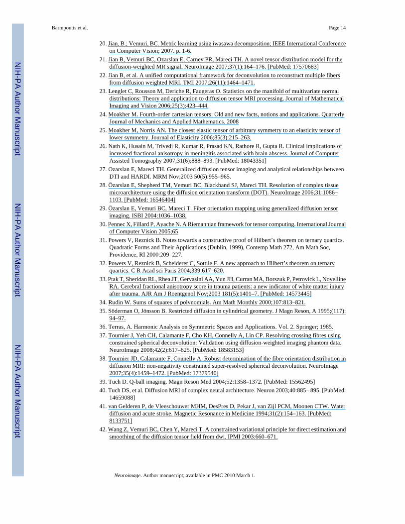
Then, we computed the displacement probability functions from the 4th-order tensors estimatedearlier using the two different methods, and after that we computed the fiber orientations fromthe maxima of these probability functions. The error angles (mean and standard deviation)between ground truth and estimated orientations from the two methods for different amountof noise in the data are plotted in Fig. 1. Here, we should emphasize that the intensity of thesimulated signal was significantly smaller when the diffusion gradient orientation formed asmall angle with the fiber orientation than that corresponding to gradient orientationsperpendicular to the fiber. These smaller intensity values are most likely to become negativewhen we corrupt the signal with noise, and as a result any method that does not impose theSPD property is affected drastically. As expected, our method yields smaller errors incomparison with the method that does not enforce the SPD property of the tensors. When weincrease the amount of noise in the data, the errors observed by the latter method aresignificantly increased, while our method depicts less sensitivity. This demonstrates the needfor enforcing the SPD property of the estimated tensors and validates the accuracy of ourproposed method.

As was expected, similar results were observed by comparing the generalized trace [13] of the4th-order diffusion tensors estimated in the previous experiment. In the case of estimating the4th-order tensors without imposing the SPD property, 44% of the estimated tensors yieldednegative generalized trace values, while the values computed using the proposed method wereall positive. In both cases we computed the standard deviation of the estimated generalizedtrace for different amounts of noise in the data (excluding from our calculations the negativevalues computed by the non SPD method). Figure 2 shows the standard deviation of thegeneralized trace computed using both the methods. By observing the figure we conclude thatthe proposed method produces significantly more accurate results even in the higher noisecases.

Furthermore, we compared the proposed parametrization of the SPD 4th-order tensors with theone presented in [1]. For the comparison, we synthesized a uniform tensor field (shown in Fig.3 left) and then we corrupted the central voxels using randomly generated 4th - order tensors.

Barmpoutis et al. Page 10

Neuroimage. Author manuscript; available in PMC 2010 March 1.

NIH

-PA Author Manuscript

NIH

-PA Author Manuscript

NIH

-PA Author Manuscript

The noisy field was regularized by minimizing ∫ ||∇Cx|| dx, where Cx are the parameters ofeach parametrization at location x (||∇Cx || was assumed to be zero at the boundary). As it wasexpected the non unique parametrization in [1] failed to produce a smooth result compared tothe proposed parametrization.

Finally, in order to compare our proposed method with other existing techniques that do notemploy 4th-order tensors, we performed another experiment using synthetic data. The datawere generated for different amounts of noise by following the same method as previouslyusing the simulated MR signal of a 2-fiber crossing. We estimated SPD 4th-order tensors fromthe corrupted simulated MR signal using our method and then computed the fiber orientationsfrom the corresponding probability functions. For comparison we also estimated the fiberorientations using the DOT method described in [28] and the ODF method presented in [39].For all three methods we computed the estimated fiber orientation errors for different amountsof noise in the data (shown in Fig. 3.1). The results conclusively demonstrate the accuracy ofour method, showing small fiber orientation errors (≃5°) for typical amount of noise with std.dev.≃ 0.5 – 0.8. Furthermore, by observing the plot, we also conclude that the accuracy of ourproposed method is very close to that of the DOT method and is significantly better than theODF method. For larger amounts of noise our method yielded smaller errors than all the othermethods.

3.2 Real data experimentsIn the following experiments, we used MR data from excised rat’s spinal cord. The protocolthat we used in this experiment included acquisition of 22 images using a pulsed gradient spinecho pulse sequence with repetition time (TR) = 1.5 s, echo time (TE) = 27.2 ms, bandwidth= 30 kHz, field-of-view (FOV) = 4.3×4.3 mm. After the first image set was collected withoutdiffusion weighting (b ~ 0 s/mm2), 21 diffusion-weighted image sets with gradient strength(G) = 664 mT/m, gradient duration (δ) = 1.5 ms, gradient separation (Δ) = 17.5 ms and diffusiontime (Td) = 17 ms were collected. The image without diffusion weighting had 8 signal averages,and each diffusion-weighted image had 2 averages.

First, we estimated an SPD 4th-order tensor field by applying the proposed method to the realDW-MRI data. Figure 5 shows the estimated elements of matrices A and B, which parameterizethe Gram matrix discussed in section 2. In the first row the estimated S0 and generalizedanisotropy [13] are also shown. The red color in the images denotes negative values. Byobserving the images we can see that each coefficient shows different details of the underlyingtissue.

Furthermore, we computed the 4th-order tensor field first without imposing the positive-definite constraint. In order to compare the obtained results with that estimated by the proposedalgorithm, in Fig. 6 we plot the corresponding tensors from a region of interest in the whitematter. In this region of interest we expected single-lobed diffusivities with peakspredominantly in the axial direction which is represented by the blue color. The X, Y, Zcomponents of the dominant orientation of each probability profile are assigned to R, G, B (red,green, blue) components of the color of each tensor. By observing this figure, we can say thatthe tensor field is incoherent if we do not enforce the SPD constraint (Fig. 6 left) and theexpected single-lobed nature of this white matter region is lost. On the other hand the tensorsobtained by our method (Fig. 6 right) are more coherent. Note that this is a result of enforcingthe SPD constraint, since in this experiment we did not use any regularization. Similarily tothe simulated data examples (Sec. 3.1), the ROI in Fig. 6 corresponds to highly anisotropicfibers in the white matter of the spinal cord, which are most likely to yield negative diffusivitieswhen the SPD property is not imposed. This demonstrates the superior performance of ouralgorithm and motivates the use of the proposed SPD constraint.

Barmpoutis et al. Page 11

Neuroimage. Author manuscript; available in PMC 2010 March 1.

NIH

-PA Author Manuscript

NIH

-PA Author Manuscript

NIH

-PA Author Manuscript

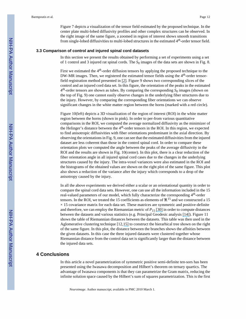
Figure 7 depicts a visualization of the tensor field estimated by the proposed technique. In thecenter plate multi-lobed diffusivity profiles and other complex structures can be observed. Inthe right image of the same figure, a zoomed in region of interest shows smooth transitionsfrom single-lobed diffusivities to multi-lobed structures in the estimated 4th-order tensor field.

3.3 Comparison of control and injured spinal cord datasetsIn this section we present the results obtained by performing a set of experiments using a setof 1 control and 3 injured rat spinal cords. The S0 images of the data sets are shown in Fig. 8.

First we estimated the 4th-order diffusion tensors by applying the proposed technique to theDW-MR images. Then, we registered the estimated tensor fields using the 4th-order tensor-field registration method presented in [2]. Figure 9 shows two corresponding slices of thecontrol and an injured cord data set. In this figure, the orientation of the peaks in the estimated4th-order tensors are shown as tubes. By comparing the corresponding S0 images (shown onthe top of Fig. 9) one cannot easily observe changes in the underlying fiber structures due tothe injury. However, by comparing the corresponding fiber orientations we can observesignificant changes in the white matter region between the horns (marked with a red circle).

Figure 10(left) depicts a 3D visualization of the region of interest (ROI) in the white matterregion between the horns (shown in pink). In order to per-from various quantitativecomparisons in the ROI, we computed the average normalized diffusivity as the minimizer ofthe Helinger’s distance between the 4th-order tensors in the ROI. In this region, we expectedto find anisotropic diffusivities with fiber orientations predominant in the axial direction. Byobserving the orientations in Fig. 9, one can see that the estimated diffusivities from the injureddataset are less coherent than those in the control spinal cord. In order to compare theseorientation plots we computed the angle between the peaks of the average diffusivity in theROI and the results are shown in Fig. 10(center). In this plot, there is a clear reduction of thefiber orientation angle in all injured spinal cord cases due to the changes in the underlyingstructures caused by the injury. The intra-voxel variances were also estimated in the ROI andthe histograms of the obtained values are shown on the right plot of the same figure. This plotalso shows a reduction of the variance after the injury which corresponds to a drop of theanisotropy caused by the injury.

In all the above experiments we derived either a scalar or an orientational quantity in order tocompare the spinal cord data sets. However, one can use all the information included in the 15real-valued parameters of our model, which fully characterize the corresponding 4th-ordertensors. In the ROI, we treated the 15 coefficients as elements of ℜ15 and we constructed a 15× 15 covariance matrix for each data set. These matrices are symmetric and positive-definiteand therefore, we can employ the Riemannian metric of P15 [30] in order to compute distancesbetween the datasets and various statistics (e.g. Principal Geodesic analysis [14]). Figure 11shows the table of Riemannian distances between the datasets. This table was then used in theAglomerative clustering technique [12,15] to construct the hierarhical tree shown on the rightof the same figure. In this plot, the distance between the branches shows the affnities betweenthe given datasets. In this case the three injured datasets were clustered together whoseRiemannian distance from the control data set is significantly larger than the distance betweenthe injured data sets.

4 ConclusionsIn this article a novel parametrization of symmetric positive semi-definite ten-sors has beenpresented using the Iwasawa decomposition and Hilbert’s theorem on ternary quartics. Theadvantage of Iwasawa components is that they can parametrize the Gram matrix, reducing theinfinite solution space caused by the Hilbert’s sum of squares parametrization. This is the first

Barmpoutis et al. Page 12

Neuroimage. Author manuscript; available in PMC 2010 March 1.

NIH

-PA Author Manuscript

NIH

-PA Author Manuscript

NIH

-PA Author Manuscript

method in literature that parametrizes the full space of the positive definite 4th-order tensors.We apply this method to estimate the diffusivity function as a field of 4th-order tensors, givena DW-MRI dataset. In the experiments presented, we used synthetic and real DW-MR imagesfrom rat spinal cords. The experimental results demonstrate the robust to noise of our methodand its superiority compared with other existing techniques.

References1. Barmpoutis, A.; Jian, B.; Vemuri, BC.; Shepherd, TM. Symmetric positive 4th order tensors and their

estimation from diffusion weighted mri. In: Karssemeijer, N.; Lelieveldt, BPF., editors. IPMI, volume4584 of Lecture Notes in Computer Science. Springer; 2007. p. 308-319.

2. Barmpoutis, A.; Vemuri, BC.; Forder, JR. Registration of high angular resolution diffusion mri imagesusing 4th order tensors . LNCS; Proceedings of MICCAI07: Int. Conf. on Medical Image Computingand Computer Assisted Intervention; Springer; 2007. p. 4791p. 908-915.

3. Barmpoutis, A.; Vemuri, BC.; Forder, JR. Fast displacement probability profile approximation fromhardi using 4th-order tensors. Proceedings of ISBI08: IEEE International Symposium on BiomedicalImaging; May 2008; p. 14-17.

4. Barmpoutis A, Vemuri BC, Shepherd TM, Forder JR. Tensor splines for interpolation andapproximation of DT-MRI with applications to segmentation of isolated rat hippocampi. TMI:Transactions on Medical Imaging November;2007 26(11):1537– 1546.

5. Basser PJ, Mattiello J, Lebihan D. Estimation of the Effective Self-Diffusion Tensor from the NMRSpin Echo. J Magn Reson B 1994;103:247–254. [PubMed: 8019776]

6. Basser PJ, Pajevic S. A normal distribution for tensor-valued random variables: Applications todiffusion tensor MRI. IEEE Trans on Medical Imaging 2003;22:785–794.

7. Basser PJ, Pajevic S. Spectral decomposition of a 4th-order covariance tensor: Applications to diffusiontensor MRI. Signal Processing 2007;87:220–236.

8. Basser PJ, Pierpaoli C. Microstructural and physiological features of tissues elucidated by quantitative-diffusion-tensor mri. J Magn Reson B 1996;111(3):209–19. [PubMed: 8661285]

9. Cercignania M, Inglesea M, Pagania E, Comia G, Filippi M. Mean diffusivity and fractional anisotropyhistograms of patients with multiple sclerosis. American Journal of Neuroradiology 2001;22:952–958.[PubMed: 11337342]

10. Chefd’Hotel C, Tschumperlé D, Deriche R, Faugeras OD. Regularizing flows for constrained matrix-valued images. J Mathematical Imaging and Vision 2004;20:147–162.

11. Descoteaux M, Angelino E, Fitzgibbons S, Deriche R. Regularized, fast and robust analytic q-ballimaging. MRM 2007;58(3):497–510.

12. Duda, RO.; Hart, PE.; Stork, DG. Pattern Classification. Wiley; 2001.13. Evren Ozarslan THM, Vemuri Baba C. Generalized scalar measures for diffusion mri using trace,

variance, and entropy. Magn Reson Med 2005;53(4):866–76. [PubMed: 15799039]14. Fletcher, P.; Joshi, S. Principal geodesic analysis on symmetric spaces: Statistics of diffusion tensors.

Proc. of CVAMIA; 2004. p. 87-98.15. Gil-Garcia, RJ.; Badia-Contelles, JM.; Pons-Porrata, A. A general framework for agglomerative

hierarchical clustering algorithms. Pattern Recognition, 2006. ICPR 2006. 18th InternationalConference on; 2006. p. 569-572.

16. Hasan KM, Gupta RK, Santos RM, Wolinsky JS, Narayana PA. Diffusion tensor fractional anisotropyof the normal-appearing seven segments of the corpus callosum in healthy adults and relapsing-remitting multiple sclerosis patients. Journal of Magnetic Resonance Imaging 2005;21(6):735–743.[PubMed: 15906348]

17. Hilbert D. Über die darstellung definiter formen als summe von formenquadraten. Math Ann1888;32:342–350.

18. Ito M, Watanabe H, Kawai Y, Atsuta N, Tanaka F, Naganawa S, Fukatsu H, Sobue G. Usefulness ofcombined fractional anisotropy and apparent diffusion coefficient values for detection of involvementin multiple system atrophy. Journal of Neurology, Neurosurgery, and Psychiatry 2007;78:722–728.

19. Iwasawa K. On some types of topological groups. The Annals of Mathematics 1949;50(3):507–558.

Barmpoutis et al. Page 13

Neuroimage. Author manuscript; available in PMC 2010 March 1.

NIH

-PA Author Manuscript

NIH

-PA Author Manuscript

NIH

-PA Author Manuscript

20. Jian, B.; Vemuri, BC. Metric learning using iwasawa decomposition; IEEE International Conferenceon Computer Vision; 2007. p. 1-6.

21. Jian B, Vemuri BC, Ozarslan E, Carney PR, Mareci TH. A novel tensor distribution model for thediffusion-weighted MR signal. NeuroImage 2007;37(1):164–176. [PubMed: 17570683]

22. Jian B, et al. A unified computational framework for deconvolution to reconstruct multiple fibersfrom diffusion weighted MRI. TMI 2007;26(11):1464–1471.

23. Lenglet C, Rousson M, Deriche R, Faugeras O. Statistics on the manifold of multivariate normaldistributions: Theory and application to diffusion tensor MRI processing. Journal of MathematicalImaging and Vision 2006;25(3):423–444.

24. Moakher M. Fourth-order cartesian tensors: Old and new facts, notions and applications. QuarterlyJournal of Mechanics and Applied Mathematics. 2008

25. Moakher M, Norris AN. The closest elastic tensor of arbitrary symmetry to an elasticity tensor oflower symmetry. Journal of Elasticity 2006;85(3):215–263.

26. Nath K, Husain M, Trivedi R, Kumar R, Prasad KN, Rathore R, Gupta R. Clinical implications ofincreased fractional anisotropy in meningitis associated with brain abscess. Journal of ComputerAssisted Tomography 2007;31(6):888–893. [PubMed: 18043351]

27. Ozarslan E, Mareci TH. Generalized diffusion tensor imaging and analytical relationships betweenDTI and HARDI. MRM Nov;2003 50(5):955–965.

28. Özarslan E, Shepherd TM, Vemuri BC, Blackband SJ, Mareci TH. Resolution of complex tissuemicroarchitecture using the diffusion orientation transform (DOT). NeuroImage 2006;31:1086–1103. [PubMed: 16546404]

29. Özarslan E, Vemuri BC, Mareci T. Fiber orientation mapping using generalized diffusion tensorimaging. ISBI 2004:1036–1038.

30. Pennec X, Fillard P, Ayache N. A Riemannian framework for tensor computing. International Journalof Computer Vision 2005;65

31. Powers V, Reznick B. Notes towards a constructive proof of Hilbert’s theorem on ternary quartics.Quadratic Forms and Their Applications (Dublin, 1999), Contemp Math 272, Am Math Soc,Providence, RI 2000:209–227.

32. Powers V, Reznick B, Scheiderer C, Sottile F. A new approach to Hilbert’s theorem on ternaryquartics. C R Acad sci Paris 2004;339:617–620.

33. Ptak T, Sheridan RL, Rhea JT, Gervasini AA, Yun JH, Curran MA, Borszuk P, Petrovick L, NovellineRA. Cerebral fractional anisotropy score in trauma patients: a new indicator of white matter injuryafter trauma. AJR Am J Roentgenol Nov;2003 181(5):1401–7. [PubMed: 14573445]

34. Rudin W. Sums of squares of polynomials. Am Math Monthly 2000;107:813–821.35. Söderman O, Jönsson B. Restricted diffusion in cylindrical geometry. J Magn Reson, A 1995;(117):

94–97.36. Terras, A. Harmonic Analysis on Symmetric Spaces and Applications. Vol. 2. Springer; 1985.37. Tournier J, Yeh CH, Calamante F, Cho KH, Connelly A, Lin CP. Resolving crossing fibres using

constrained spherical deconvolution: Validation using diffusion-weighted imaging phantom data.NeuroImage 2008;42(2):617–625. [PubMed: 18583153]

38. Tournier JD, Calamante F, Connelly A. Robust determination of the fibre orientation distribution indiffusion MRI: non-negativity constrained super-resolved spherical deconvolution. NeuroImage2007;35(4):1459–1472. [PubMed: 17379540]

39. Tuch D. Q-ball imaging. Magn Reson Med 2004;52:1358–1372. [PubMed: 15562495]40. Tuch DS, et al. Diffusion MRI of complex neural architecture. Neuron 2003;40:885– 895. [PubMed:

14659088]41. van Gelderen P, de Vleeschouwer MHM, DesPres D, Pekar J, van Zijl PCM, Moonen CTW. Water

diffusion and acute stroke. Magnetic Resonance in Medicine 1994;31(2):154–163. [PubMed:8133751]

42. Wang Z, Vemuri BC, Chen Y, Mareci T. A constrained variational principle for direct estimation andsmoothing of the diffusion tensor field from dwi. IPMI 2003:660–671.

Barmpoutis et al. Page 14

Neuroimage. Author manuscript; available in PMC 2010 March 1.

NIH

-PA Author Manuscript

NIH

-PA Author Manuscript

NIH

-PA Author Manuscript

43. Wang Z, Vemuri BC, Chen Y, Mareci TH. A constrained variational principle for direct estimationand smoothing of the diffusion tensor field from complex dwi. IEEE Trans Med Imaging 2004;23(8):930–939. [PubMed: 15338727]

44. Ward P, Counsell S, Allsop J, Cowan F, Shen Y, Edwards D, Scia M, Rutherford M. Reducedfractional anisotropy on diffusion tensor magnetic resonance imaging after hypoxicischemicencephalopathy. Pediatrics 2006;117(4):619–630.

Barmpoutis et al. Page 15

Neuroimage. Author manuscript; available in PMC 2010 March 1.

NIH

-PA Author Manuscript

NIH

-PA Author Manuscript

NIH

-PA Author Manuscript

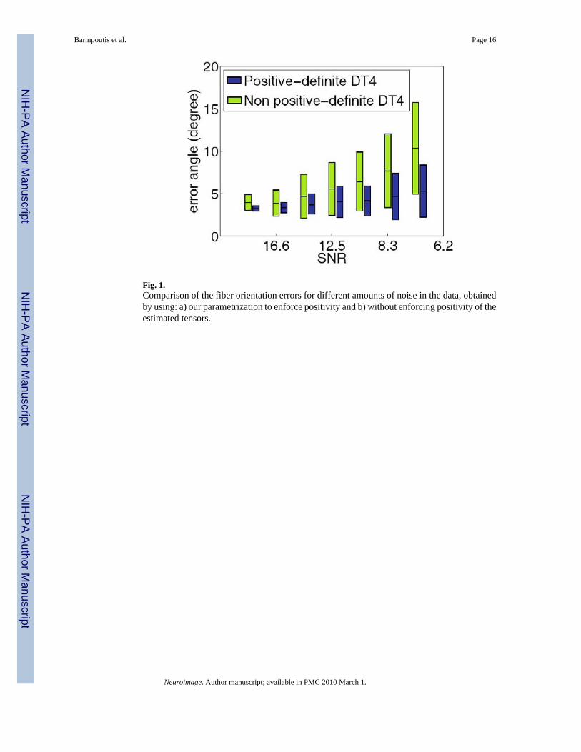
Fig. 1.Comparison of the fiber orientation errors for different amounts of noise in the data, obtainedby using: a) our parametrization to enforce positivity and b) without enforcing positivity of theestimated tensors.

Barmpoutis et al. Page 16

Neuroimage. Author manuscript; available in PMC 2010 March 1.

NIH

-PA Author Manuscript

NIH

-PA Author Manuscript

NIH

-PA Author Manuscript

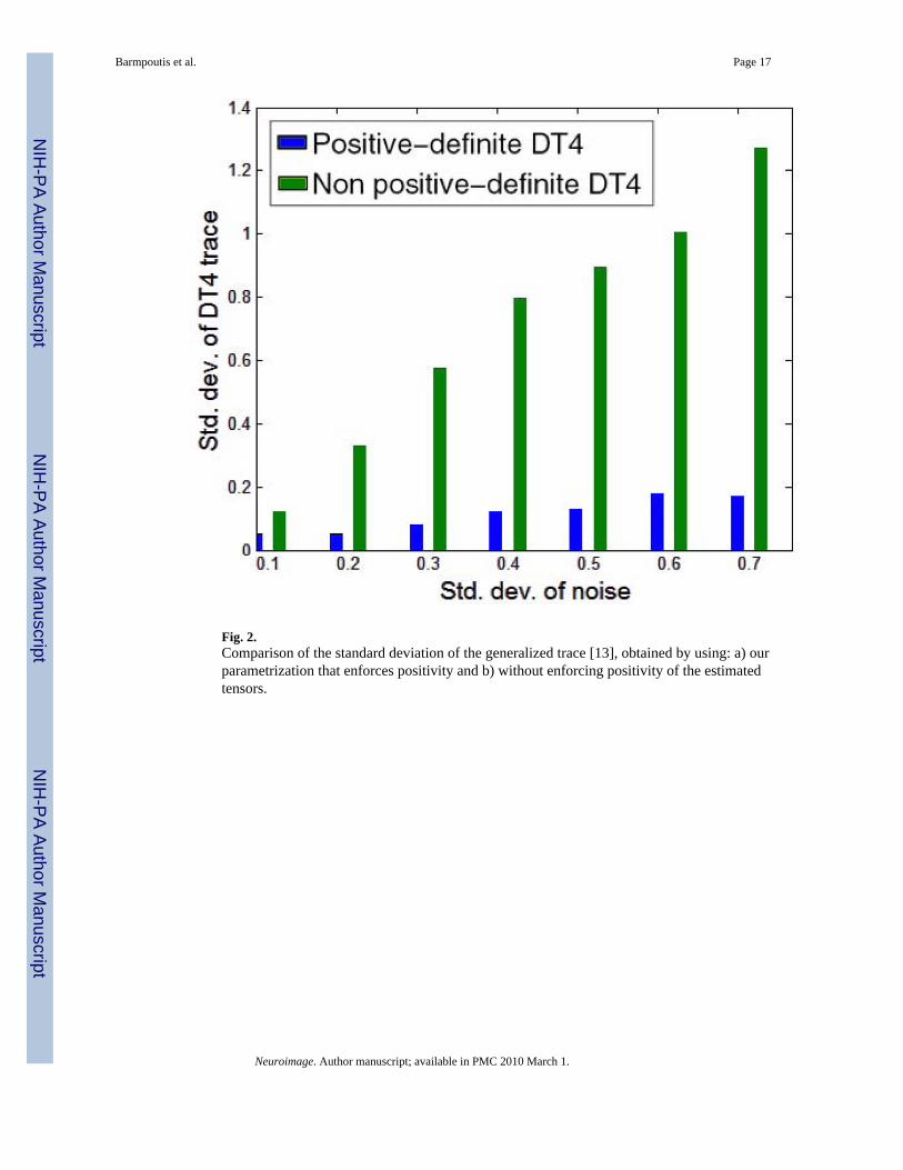
Fig. 2.Comparison of the standard deviation of the generalized trace [13], obtained by using: a) ourparametrization that enforces positivity and b) without enforcing positivity of the estimatedtensors.

Barmpoutis et al. Page 17

Neuroimage. Author manuscript; available in PMC 2010 March 1.

NIH

-PA Author Manuscript

NIH

-PA Author Manuscript

NIH

-PA Author Manuscript

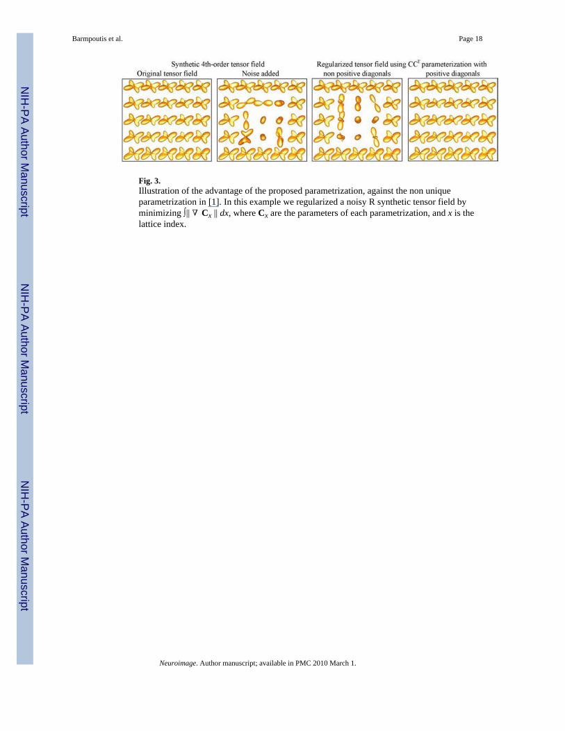
Fig. 3.Illustration of the advantage of the proposed parametrization, against the non uniqueparametrization in [1]. In this example we regularized a noisy R synthetic tensor field byminimizing ∫|| ∇ Cx || dx, where Cx are the parameters of each parametrization, and x is thelattice index.

Barmpoutis et al. Page 18

Neuroimage. Author manuscript; available in PMC 2010 March 1.

NIH

-PA Author Manuscript

NIH

-PA Author Manuscript

NIH

-PA Author Manuscript

Fig. 4.Fiber orientation errors for different SNR in the data using our method for the estimation ofpositive 4th-order tensors and two other existing methods: 1) DOT and 2) ODF.

Barmpoutis et al. Page 19

Neuroimage. Author manuscript; available in PMC 2010 March 1.

NIH

-PA Author Manuscript

NIH

-PA Author Manuscript

NIH

-PA Author Manuscript

Fig. 5.The elements of matrices A and B estimated by the proposed method as well the estimatedS0 and generalized anisotropy [13].

Barmpoutis et al. Page 20

Neuroimage. Author manuscript; available in PMC 2010 March 1.

NIH

-PA Author Manuscript

NIH

-PA Author Manuscript

NIH

-PA Author Manuscript

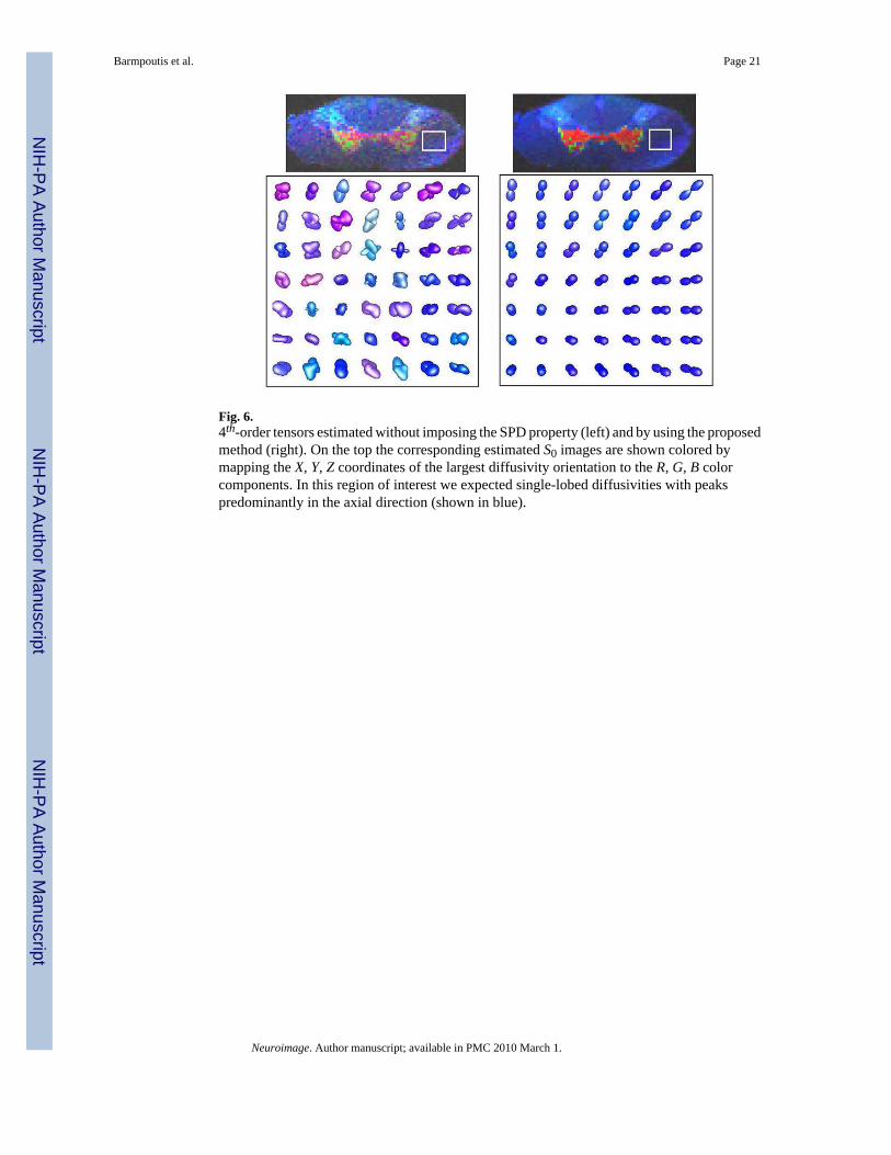
Fig. 6.4th-order tensors estimated without imposing the SPD property (left) and by using the proposedmethod (right). On the top the corresponding estimated S0 images are shown colored bymapping the X, Y, Z coordinates of the largest diffusivity orientation to the R, G, B colorcomponents. In this region of interest we expected single-lobed diffusivities with peakspredominantly in the axial direction (shown in blue).

Barmpoutis et al. Page 21

Neuroimage. Author manuscript; available in PMC 2010 March 1.

NIH

-PA Author Manuscript

NIH

-PA Author Manuscript

NIH

-PA Author Manuscript

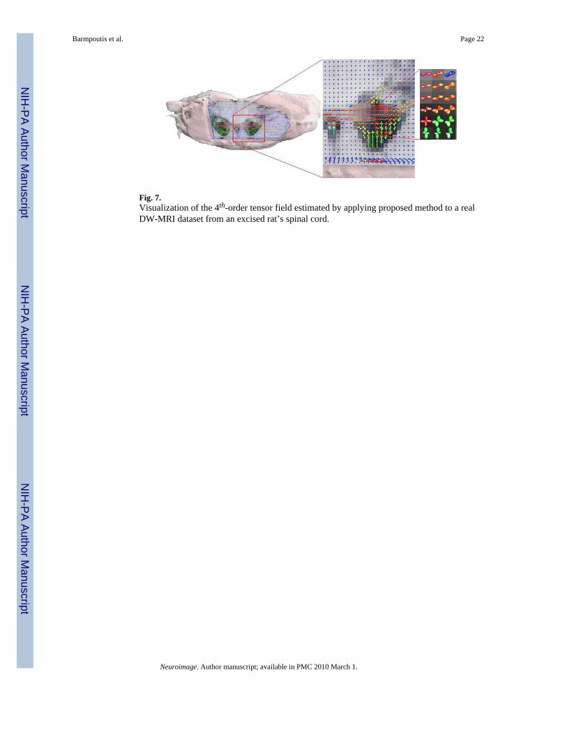
Fig. 7.Visualization of the 4th-order tensor field estimated by applying proposed method to a realDW-MRI dataset from an excised rat’s spinal cord.

Barmpoutis et al. Page 22

Neuroimage. Author manuscript; available in PMC 2010 March 1.

NIH

-PA Author Manuscript

NIH

-PA Author Manuscript

NIH

-PA Author Manuscript

Fig. 8.The acquired S0 image of a control (left) and three injured rat spinalcords.

Barmpoutis et al. Page 23

Neuroimage. Author manuscript; available in PMC 2010 March 1.

NIH

-PA Author Manuscript

NIH

-PA Author Manuscript

NIH

-PA Author Manuscript

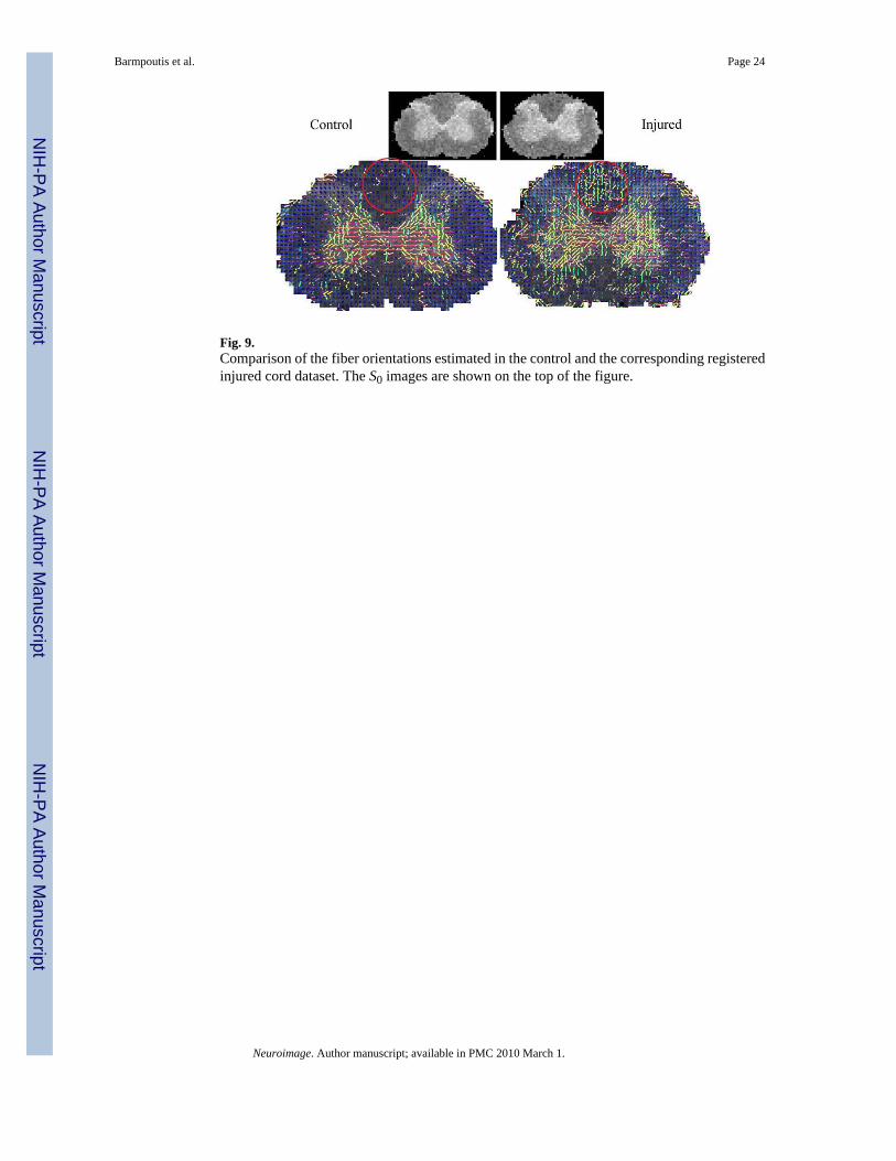
Fig. 9.Comparison of the fiber orientations estimated in the control and the corresponding registeredinjured cord dataset. The S0 images are shown on the top of the figure.

Barmpoutis et al. Page 24

Neuroimage. Author manuscript; available in PMC 2010 March 1.

NIH

-PA Author Manuscript

NIH

-PA Author Manuscript

NIH

-PA Author Manuscript

Fig. 10.Visualization of the ROI (shown in pink) in 3D. The plots show comparisons between the fiberorientation angle of the average diffusivity in the ROI and the histogram of variances in theROI.

Barmpoutis et al. Page 25

Neuroimage. Author manuscript; available in PMC 2010 March 1.

NIH

-PA Author Manuscript

NIH

-PA Author Manuscript

NIH

-PA Author Manuscript

Fig. 11.Quantitative comparison of the rat spinal cord dataset using the Rie-mannian metric of the 15× 15 positive definite matrices. The Riemannian distances between the covariance matricesare shown on the left. The corresponding hierarchical dendrogram computed using theRiemannian distances.

Barmpoutis et al. Page 26

Neuroimage. Author manuscript; available in PMC 2010 March 1.

NIH

-PA Author Manuscript

NIH

-PA Author Manuscript

NIH

-PA Author Manuscript

NIH

-PA Author Manuscript

NIH

-PA Author Manuscript

NIH

-PA Author Manuscript

Barmpoutis et al. Page 27

Table 1Formulas to compute the tensor coefficients Di,j,k given the components a11, a22,a33, a21, a31, a32, b11, b12, b13, b21, b22, b23, b31, b32, b33 and the fixed parameterc = 10−308.

D400 = a112 + c

D040 = a212 + a22

2 + c

D004 = a312 + a32

2 + a332 + c

D220 = b112 + b12

2 + b132 + 2 a11 a21 + 2c

D202 = b212 + b22

2 + b232 + 2 a11 a31 + 2c

D022 = b312 + b32

2 + b332 + 2 a21 a31 + 2 a22 a32 + 2c

D310 = 2 a11 b11

D301 = 2 a11 b21

D130 = 2(a21 b11 + a22 b12)

D031 = 2(a21 b31 + a22 b32)

D103 = 2(a31 b21 + a32 b22 + a33 b23)

D013 = 2(a31 b31 + a32 b32 + a33 b33)

D211 = 2(b11 b21 + b12 b22 + b13 b23 + a11 b31)

D121 = 2(b11 b31 + b12 b32 + b13 b33 + a21 b21 + a22 b22)

D112 = 2(b21 b31 + b22 b32 + b23 b33 + a31 b11 + a32 b12 + a33 b13)

Neuroimage. Author manuscript; available in PMC 2010 March 1.