ABSTRACT

Glazman-Krein-Naimark Theory, Left-Definite Theory, and the Square of theLegendre Polynomials Differential Operator

Quinn Callahan Wicks, Ph.D.

Advisors: Lance L. Littlejohn, Ph.D. and Constanze Liaw, Ph.D.

As an application of a general left-definite spectral theory, Everitt, Littlejohn

and Wellman, in 2002, developed the left-definite theory associated with the clas-

sical Legendre self-adjoint second-order differential operator A in L2(−1, 1) which

has the Legendre polynomials {Pn}∞n=0 as eigenfunctions. As a consequence, they

explicitly determined the domain D(A2) of the self-adjoint operator A2. However,

this domain, in their characterization, does not contain boundary conditions in its

formulation. In fact, this is a general feature of the left-definite approach developed

by Littlejohn and Wellman. Yet, the square of the second-order Legendre expres-

sion is in the limit-4 case at each endpoint x = ±1 in L2(−1, 1), so D(A2) should

exhibit four boundary conditions. In this thesis, we show that this domain can, in

fact, be expressed using four separated boundary conditions using the classical GKN

(Glazman-Krein-Naimark) theory. In addition, we determine a new characterization

of D(A2) that involves four non-GKN boundary conditions. These new boundary

conditions are surprisingly simple and natural, and are equivalent to the boundary

conditions obtained from the GKN theory.

Glazman-Krein-Naimark Theory, Left-Definite Theory, and the Square of theLegendre Polynomials Differential Operator

by

Quinn Callahan Wicks, B.A., M.S.

A Dissertation

Approved by the Department of Mathematics

Lance L. Littlejohn, Ph.D., Chairperson

Submitted to the Graduate Faculty ofBaylor University in Partial Fulfillment of the

Requirements for the Degreeof

Doctor of Philosophy

Approved by the Dissertation Committee

Lance L. Littlejohn, Ph.D., Co-Chairperson

Constanze Liaw, Ph.D., Co-Chairperson

Klaus Kirsten, Ph.D.

Brian Simanek, Ph.D.

James Stamey, Ph.D.

Accepted by the Graduate SchoolMay 2016

J. Larry Lyon, Ph.D., Dean

Page bearing signatures is kept on file in the Graduate School.

Copyright c© 2016 by Quinn Callahan Wicks

All rights reserved

TABLE OF CONTENTS

LIST OF FIGURES vi

LIST OF TABLES vii

ACKNOWLEDGMENTS viii

DEDICATION ix

1 Introduction 1

2 Legendre Polynomials and the Legendre Differential Equation 6

2.1 Definition and Properties of Orthogonal Polynomials . . . . . . . . . 6

2.2 The Classical Systems of Orthogonal Polynomials . . . . . . . . . . . 8

2.3 The Legendre Polynomials and the Legendre Differential Equation . . 12

3 The GKN Theory of Self-Adjoint Extensions of Symmetric Operators 14

3.1 Symmetric Operators . . . . . . . . . . . . . . . . . . . . . . . . . . . 14

3.2 Weyl Theory . . . . . . . . . . . . . . . . . . . . . . . . . . . . . . . 15

3.3 Extensions of General Symmetric Operators . . . . . . . . . . . . . . 18

3.4 Extensions of Symmetric Differential Operators . . . . . . . . . . . . 21

3.5 Glazman-Krein-Naimark (GKN) Theory . . . . . . . . . . . . . . . . 25

3.6 The Method of Frobenius . . . . . . . . . . . . . . . . . . . . . . . . 26

4 Properties and Restrictions of the Maximal Domain 29

4.1 Properties of the Maximal Domain of `[·] . . . . . . . . . . . . . . . . 30

4.2 Properties of a Restriction of the Maximal Domain . . . . . . . . . . 33

4.3 The Right-Definite Problem . . . . . . . . . . . . . . . . . . . . . . . 35

iv

5 The Legendre Polynomials Self-Adjoint Operator A 38

5.1 Hilbert Function Spaces . . . . . . . . . . . . . . . . . . . . . . . . . 42

5.2 The Legendre Differential Operator A in L2(−1, 1) . . . . . . . . . . . 44

5.3 Equivalent Properties of the Domain D(A) . . . . . . . . . . . . . . . 47

5.4 Other Self-Adjoint Operators in L2(−1, 1) . . . . . . . . . . . . . . . 50

5.5 The Legendre Differential Operator S in H21 (−1, 1) . . . . . . . . . . 50

6 Littlejohn-Wellman Left-Definite Theory with Applications to the LegendrePolynomials Operator 54

6.1 Introduction and Motivation . . . . . . . . . . . . . . . . . . . . . . . 54

6.2 The Definition of a Left-Definite Space and Operator . . . . . . . . . 58

6.3 Main Theorems . . . . . . . . . . . . . . . . . . . . . . . . . . . . . . 60

6.4 The Spectral Theorem . . . . . . . . . . . . . . . . . . . . . . . . . . 65

6.5 Left-Definite Theory and the Legendre Polynomials Operator . . . . . 68

6.6 The Legendre-Stirling Numbers . . . . . . . . . . . . . . . . . . . . . 68

7 The Square of the Legendre Polynomials Operator 71

7.1 A GKN Self-Adjoint Operator Generated by the Square of the Leg-endre Differential Expression . . . . . . . . . . . . . . . . . . . . . . . 71

7.2 Statements of the Main Theorems . . . . . . . . . . . . . . . . . . . . 78

7.3 A Key Integral Inequality . . . . . . . . . . . . . . . . . . . . . . . . 79

7.4 Proof of Theorem 7.3 . . . . . . . . . . . . . . . . . . . . . . . . . . . 81

7.5 Proof of Theorem 7.4 . . . . . . . . . . . . . . . . . . . . . . . . . . . 88

7.6 Proof of Theorem 7.5 . . . . . . . . . . . . . . . . . . . . . . . . . . . 94

8 The nth Power of the Legendre Polynomials Operator 98

BIBLIOGRAPHY 103

v

LIST OF FIGURES

1.1 The only known image of Adrien-Marie Legendre [16] . . . . . . . . . 5

2.1 Five Legendre polynomials . . . . . . . . . . . . . . . . . . . . . . . . 13

vi

LIST OF TABLES

6.1 Some Legendre-Stirling numbers . . . . . . . . . . . . . . . . . . . . . 70

7.1 Calculation of some sesquilinear forms . . . . . . . . . . . . . . . . . 74

vii

ACKNOWLEDGMENTS

Were it not for Dr. Lance Littlejohn, I would never have acheived my goal of

completing my Ph.D. in mathematics. When I first visited the Baylor Mathematics

Department with my 5-month-old son in early 2010, he welcomed me. That fall, he

taught my first true graduate real analysis course. Not long after, he enthusiastically

accepted me as his Ph.D. student even when he had just started with another – my

“math sister” and close friend Dr. Jessica Stewart Kelly. In the last three years, he

has not only persevered through the midst of his additional duties as Associate Dean

of Research for the Graduate School, but has patiently endured all my globetrotting.

Dr. Littlejohn, I cannot thank you enough.

Though I left not long after she came to Baylor, Dr. Constanze Liaw kept

my hope alive long-distance by spending countless hours of her own precious time

encouraging and guiding me in this project. I am forever indebted to Dr. Liaw for

her support and knowledge.

I would like to thank my committee members Drs. Klaus Kirsten, Brian

Simanek, and James Stamey for their involvement and insightful comments. I would

also like to thank Rita Massey, Judy Dees, and Margaret Salinas for all their hard

work and patience.

A special thank-you goes to Dr. Ronald Stanke, and another to Dr. Matthew

Beauregard. I would also like to thank my fellow graduate students Adam Anderson

and Drs. James Kelly, Charles Nelms, Dylan Poulsen, and Brian Streit, who made

my time at Baylor so enjoyable. Jessica, words cannot express how grateful I am for

your continued friendship and support.

With deepest gratitude I thank my mother and father, who have encouraged

and supported me every day of my life, and my sweet husband, who makes it all

worth it.

viii

DEDICATION

For my family

ix

CHAPTER ONE

Introduction

The analytical study of the classical second-order Legendre differential expres-

sion

`[y](x) = −((1− x2)y′(x)

)′has a long and rich history stretching back to the seminal work of Weyl in 1910 [68]

and Titchmarsh in 1940 [64]. Part, if not most, of the reason for the importance of

this second-order expression lies in the fact that the Legendre polynomials {Pn}∞n=0

are solutions. More specifically, the Legendre polynomial y = Pn(x), for n ∈ N0, is

a solution of the eigenvalue equation

`[y](x) = n(n+ 1)y(x).

In the Hilbert space L2(−1, 1), there is a continuum of self-adjoint operators gen-

erated by `[·]. One such operator A stands out from the rest: this is the Legen-

dre polynomials operator, so named because the Legendre polynomials {Pn}∞n=0 are

eigenfunctions of A. We review properties of this operator in chapter six.

In the mid-1970s, A. Pleijel wrote two papers (see [55] and [56]) on the Legen-

dre expression from a left-definite spectral point of view. Everitt’s contribution [19]

continued this left-definite study in addition to detailing an in-depth analysis of the

Legendre expression in the right-definite setting L2(−1, 1) where he discovered new

properties of functions in the domain D(A) of A. In [42], A. M. Krall and Littlejohn

considered properties of the Legendre expression under the left-definite energy norm.

In 2000, Vonhoff extended Everitt’s results in [66] with an extensive study of `[·] in

its (first) left-definite setting. In 2002, Everitt, Littlejohn, and Maric [24] published

further results in which they gave several equivalent conditions for functions to be-

long to D(A); this result is given below in Theorem 5.6. We also refer the reader to

1

the paper [49] by Littlejohn and Zettl where the authors determine all self-adjoint

operators, generated by the Legendre expression `[·], in the Hilbert spaces L2(−1, 1),

L2(−∞,−1), L2(1,∞), and L2(R).

Littlejohn and Wellman [47], in 2002, developed a general left-definite theory

for an unbounded self-adjoint operator T bounded below by a positive constant in a

Hilbert space H = (V, (·, ·)), where V denotes the underlying (algebraic) vector space

and H is the resulting topological space induced by the inner product (·, ·). To sum-

marize, the authors construct a continuum of Hilbert spaces {Hr = (Vr, (·, ·)r)}r>0,

forming a Hilbert scale, generated by positive powers of T . The authors called these

Hilbert spaces left-definite spaces ; they are constructed using the Hilbert space spec-

tral theorem (see [58]) for self-adjoint operators.

It is a difficult problem, in general, to explicitly determine the domain of a

power of an unbounded operator. However, the authors in [47] prove that Vr =

D(Tr2 ) and (f, g)r = (T

r2f, T

r2 g). Furthermore, in many practical applications, as

the authors demonstrate in [47], the computation of the vector spaces Vr and inner

products (·, ·)r is surprisingly not difficult. In a subsequent paper, Everitt, Little-

john, and Wellman [25] applied this theory to the Legendre polynomials operator

A. Among other results, the authors explicitly compute the domains of D(An2 ) for

each n ∈ N. Specifically, they proved that

D(An2 ) = {f : (−1, 1)→ C | f, f ′, ..., f (n−1) ∈ ACloc(−1, 1);

(1− x2)n2 f (n) ∈ L2(−1, 1)} (n ∈ N).

(1.1)

In particular, we see that D(A2) is explicitly given by

B = {f : (−1, 1)→ C | f, f ′, f ′′, f ′′′ ∈ ACloc(−1, 1); (1− x2)2f (4) ∈ L2(−1, 1)};

(1.2)

the reason for using the notation B, instead of D(A2), will be made clear shortly.

Of course, for f ∈ B, we have A2f = `2[f ], where `2[·] is the square of the Legendre

2

differential expression given by

`2[y](x) =((1− x2)2y′′(x)

)′′ − 2((1− x2)y′(x)

)′= (1− x2)2y(4)(x)− 8x(1− x2)y′′′(x) + (14x2 − 6)y′′(x) + 4xy′(x).

(1.3)

Notice that, curiously, there are no “boundary conditions” given in (1.2). From the

Glazman-Krein-Naimark (GKN) theory (see [52]), there should be four such bound-

ary conditions. This begs an obvious question: how can we “extract” boundary

conditions from the representation of D(A2) in (1.2)? In this thesis, we will answer

this question. It is interesting that the condition (1 − x2)2f (4) ∈ L2(−1, 1) seems

to “encode” these boundary conditions. In fact, along the way, we will characterize

D(A2) in four different ways. Of course, we have the algebraic definition

D(A2) := {f ∈ D(A) | Af ∈ D(A)} (1.4)

(we will show that D(A2), given in (1.4), is equal to B, defined in (1.2)). We will

also prove that D(A2) is characterized by GKN boundary conditions associated with

a self-adjoint operator S, generated by `2[·], in L2(−1, 1). Specifically, we prove that

D(A2) is equal to

D(S) := {f : (−1, 1)→ C | f, f ′, f ′′, f ′′′ ∈ ACloc(−1, 1); f, `2[f ] ∈ L2(−1, 1);

limx→±1

[f, 1]2(x) = 0; limx→±1

[f, x]2(x) = 0},(1.5)

where [·, ·]2 is the sesquilinear form associated with Green’s formula and `2[·] in

L2(−1, 1); this form will be defined in Section 7.1. In this thesis, we also show that

D(A2) is equal to

D := {f : (−1, 1)→ C | f, f ′, f ′′, f ′′′ ∈ ACloc(−1, 1); f, `2[f ] ∈ L2(−1, 1);

limx→±1

(1− x2)f ′(x) = 0; limx→±1

((1− x2)2f ′′(x)

)′= 0}.

(1.6)

This characterization of D(A2) is surprising since the boundary conditions in (1.6)

are not GKN boundary conditions; we say that D is a GKN-like domain. The

3

boundary conditions in (1.6) are remarkably simple; indeed, they are obtained as

limits from each of the two terms in (1.3) minus one derivative.

In [12], the authors first showed the smoothness condition

f ∈ D(A) =⇒ f ′ ∈ L2(−1, 1). (1.7)

As a consequence of our results in this thesis, we are able to generalize (1.7) by

proving

f ∈ D(A2) =⇒ f ′′ ∈ L2(−1, 1) and `[f ] ∈ AC[−1, 1];

see Corollary 7.11 below.

The contents of this thesis are as follows. In chapter two, we discuss the Legen-

dre polynomials in the context of orthogonal polynomials systems and the Legendre

expression. In chapter three, we explain GKN theory in general as well as Weyl

theory and the method of Frobenius, all of which are essential to the GKN analy-

sis of the Legendre polynomials operator. In chapter four we discuss the maximal

domain of the Legendre operator. In chapter five, we apply GKN theory to find

all the self-adjoint extensions of the minimal operator associated with the Legendre

differential expression, and then focus on the properties of the particular self-adjoint

extension that has the Legendre polynomials as eigenfunctions. This gives context

for Theorem 5.6, which lists all the known equivalent conditions for a function to

be in the domain of the Legendre operator. We also briefly look at the Legendre

differential operator in the left-definite Hilbert-Sobolev function space H21 (−1, 1),

which paves the way for the discussion of Littlejohn-Wellman left-definite theory in

chapter six. In chapter seven, we define and prove that the four various ways to

define the domain of the operator A2, are all equal; i.e.,

• B, the left-definite domain given in (1.2),

• D(A2), the algebraic definition of the domain given in (1.4),

4

• D(S), the domain of the self-adjoint operator S (which turns out to be A2)

defined by GKN theory given in (1.5), and

• D, the domain given by non-GKN boundary conditions given in (1.6) which

most resembles the original domain for the Legendre polynomials operator,

D(A),

are equivalent. We first define the above four domains in Sections 7.1 and 7.2.

Then, a key and indispensable analytic tool used in the proofs of these theorems,

called the Chisholm-Everitt (CE) theorem, is discussed in Section 7.3. The proofs

of the theorems in Sections 7.4 through 7.6 establish our main result, Theorem 7.12.

Finally, in chapter eight, we conjecture a generalization of our main results.

One final remark: to summarize, in this thesis we show that our left-definite

characterization (1.2) of D(A2) can be rewritten as a GKN domain (Theorem 7.6)

and as a GKN-like domain (Theorem 7.12). Presumably, techniques developed in

this paper will establish, for n ∈ N, that the left-definite characterization D(An),

given in (1.1), can be expressed as both a GKN domain and a GKN-like domain.

However, it is important to note—see (1.1)—that the left-definite theory also explic-

itly determines the domains D(An2 ) of A

n2 for odd, positive, integers n. The GKN

theory was not built to handle these operators or domains.

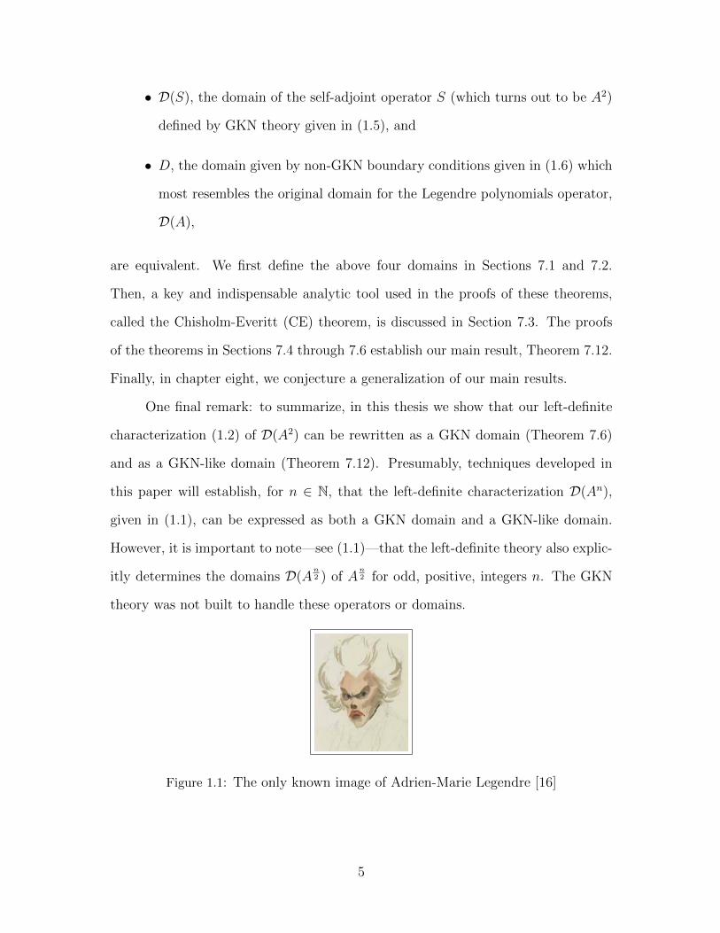
Figure 1.1: The only known image of Adrien-Marie Legendre [16]

5

CHAPTER TWO

Legendre Polynomials and the Legendre Differential Equation

2.1 Definition and Properties of Orthogonal Polynomials

Let {µn}∞n=0 be a sequence of complex numbers. A complex-valued linear

functional L defined on the vector space of all polynomials with complex coefficients

by L[xn] = µn, n ∈ N0, is called the moment functional determined by the moment

sequence {µn}. The number µn is called the moment of order n. A sequence {pn}∞n=0

of polynomials is called an orthogonal polynomial sequence with respect to some

moment functional L if for all nonnegative integers m and n,

(i) pn(x) is a polynomial of degree n

(ii) L(pnpm) = 0 when m 6= n, and

(iii) L(p2n) 6= 0.

If, in addition, we also have L(p2n) = 1, n ∈ N0, then {pn}∞n=0 is an orthonormal

polynomial sequence.

Of course, not every sequence of complex numbers determines a moment func-

tional having an orthogonal polynomial sequence. For n ∈ N0, let

∆n = det (µi+j)ni,j=0 =

∣∣∣∣∣∣∣∣∣∣∣∣∣

µ0 µ1 · · · µn

µ1 µ2 · · · µn+1

......

...

µn µn+1 · · · µ2n

∣∣∣∣∣∣∣∣∣∣∣∣∣for n ∈ N0. A moment functional L is quasi-definite if ∆n 6= 0 for all n ∈ N0.

A moment function L is called positive-definite if L[p(x)] > 0 for every poly-

nomial p(x) which is non-negative for all real x and not identically 0. We have the

following important characterization of positive-definite moment functionals:

6

Theorem 2.1. A moment functional L is positive-definite if and only if its moments

are all real and ∆n > 0 for each n ∈ N0.

Proof. See [11].

One of the most important characteristics of orthogonal polynomials in our

setting is that they satisfy a three-term recurrence formula. More specifically, we

have the following theorem:

Theorem 2.2. Let L be a moment functional with orthogonal polynomial sequence

{pn(x)}. Then there exist constants An, Bn, and Cn, where An 6= 0 and Cn 6= 0,

such that

pn+1(x) = (Anx+Bn)pn(x)− Cnpn−1(x)

for n ∈ N0, where we define p−1(x) := 0.

Remarkably, the converse of Theorem 2.2 is true and is known as Favard’s

theorem. We also have the following, known as Boas’ moment theorem.

Theorem 2.3. Let {µn} be an arbitrary sequence of real numbers. Then there is a

function ϕ of bounded variation on (−∞,∞) such that for n ∈ N0,∫ ∞−∞

xndϕ(x) = µn.

Proof. See [9].

In the case of a moment functional L with complex moments, a generalization

of Boas’ theorem shows that L can be represented by a complex-valued function

of bounded variation. It should be noted that the function ϕ in Theorem 2.3 is

not unique since we can always add a function of bounded variation to ϕ with the

property that all of its moments are zero. In addition, though Boas’ theorem is an

important theoretical result, its proof is not constructive. In practice it is difficult

to find a weight function for a given moment sequence [50].

7

The following theorem will be referred to below in chapter four.

Theorem 2.4. Let α(x) be a nondecreasing function which is not constant on the

compact interval [a, b]. Assume {pn(x)} is an orthogonal polynomial sequence with

respect to the distribution dα(x) on [a, b]. Then {pn(x)} is a complete orthogonal

polynomial sequence in L2α[a, b] where

L2α[a, b] = {f : [a, b]→ C | f is measurable with respect to α

and

∫ b

a

|f(x)|2dα(x) <∞}.

Proof. See [63].

2.2 The Classical Systems of Orthogonal Polynomials

In 1929, Bochner [10] classified all orthogonal polynomial solutions to the

second order equation

an(x)y′′(x) + a1(x)y′(x) + a0(x)y(x) = λy(x), (2.1)

where a2, a1, and a0 are polynomials and λ is a parameter independent of x. He

observed that if (2.1) has a polynomial solution of degree m, m = 0, 1, 2, then a2, a1,

and a0 were of degrees at most 2, 1, and 0, respectively. By considering the possible

locations of the roots of a2, Bochner concluded that the only polynomial solutions

(up to a linear change of variables) are

(i) the Jacobi polynomials {P (α,β)n }∞n=0, where −α,−β,−(α + β + 1) 6∈ N;

(ii) the Laguerre polynomials {L(α)n }∞n=0, where −α 6∈ N;

(iii) the Hermite polynomials {Hn}∞n=0;

(iv) the Bessel polynomials {yan}∞n=0, where −(a+ 1) 6∈ N;

(v) and {xn}∞n=0.

8

(There is clear evidence that Bochner knew of the existence of the Bessel orthogonal

polynomial sequence, though these polynomials were not officially discovered until

1948.) The polynomials in (5), however, cannot form an orthogonal polynomial

sequence with respect to any moment functional L since 0 6= L(x2x2) = L(xx3) =

0. Thus, the only orthogonal polynomials that are solutions to a second order

differential equation of the form (2.1) are the classical orthogonal polynomials of

Jacobi, Laguerre, and Hermite, together with the Bessel polynomials. We call these

four sequences of polynomials the Bochner-Krall orthogonal polynomials of order 2.

Another important classification theorem was given by Hahn [29], who showed

that if {pn}∞n=0 and {p′n}∞n=0 are orthogonal polynomial sequences with respect to

positive-definite moment functionals, then {pn}∞n=0 is (up to a linear change of vari-

able) one of the three classical systems of orthogonal polynomials. It was later

observed by Krall [44] and Beale [7] that the only orthogonal polynomial sequences

whose derivatives form an orthogonal polynomial sequence with respect to a quasi-

definite moment functional are the classical orthogonal polynomials and the Bessel

polynomials.

A third characterization of these polynomials was suggested by Tricomi [65]

and a complete proof was given by Ebert [17] and Cryer [13]. They proved that the

only polynomial sequences that have Rodrigues formulas are the Hermite, Laguerre,

Jacobi, and Bessel polynomals. By a Rodrigues formula we mean a formula of the

form

pn(x) = K−1n [w(x)]−1Dn[ρn(x)w(x)], n ∈ N0,

where

(i) Kn is independent of x;

(ii) ρ(x) is a polynomial independent of n;

(iii) w(x) is positive and integrable over some interval (a, b).

9

Several orthogonal polynomial sequences can be found through generating

functions. A generating function for {pn}∞n=0 is a function F of two variables such

that

F (x,w) =∞∑n=0

anpn(x)wn,

where convergence is in some region of the plane R2 and {an} is a known sequence

of constants.

The Jacobi polynomials {P (α,β)n }, where α > −1 and β > −1, are the classical

system of orthogonal polynomials for which the Legendre polynomials are a special

case. The explicit formula for the nth Jacobi polynomial is

P (α,β)n (x) = 2−n

n∑k=0

(n+ α

n− k

)(n+ β

k

)(x− 1)k(x+ 1)n−k (n ∈ N0).

The Jacobi polynomials are the eigenfunctions of the differential equation [48]

(1− x2)y′′(x) + [β − α− (α + β + 2)x]y′(x) + n(n+ α + β + 1)y(x) = λny(x),

where λn = n(n + α + β + 1). These polynomials are orthogonal on [−1, 1] with

respect to the weight function w(x) = (1− x)α(1 + x)β and∫ 1

−1P (α,β)m (x)P (α,β)

n (x)w(x)dx =2α+β+1Γ(n+ α + 1)Γ(n+ β + 1)

(2n+ α + β1)Γ(n+ α + β + 1)n!δmn,

where Γ denotes the Gamma function (use of the Γ symbol is also credited to Leg-

endre) and δmn denotes Dirac’s δ-function.

The Rodrigues Formula for the Jacobi polynomials is

P (α,β)n (x) = (−2)−n(n!)−1(1− x)−α(1 + x)−β

dn

dxn[(1− x)n+α(1 + x)n+β],

and a generating function is

2α+βR−1(1− x+R)−α(1 + w +R)−β =∞∑n=0

P (α,β)n (x)wn,

10

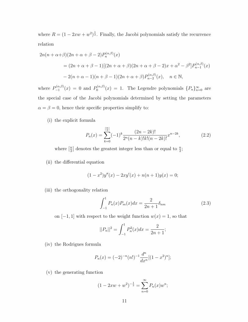
where R = (1− 2xw + w2)12 . Finally, the Jacobi polynomials satisfy the recurrence

relation

2n(n+ α+β)(2n+ α + β − 2)P (α,β)n (x)

= (2n+ α + β − 1)[(2n+ α + β)(2n+ α + β − 2)x+ α2 − β2]P(α,β)n−1 (x)

− 2(n+ α− 1)(n+ β − 1)(2n+ α + β)P(α,β)n−2 (x), n ∈ N,

where P(α,β)−1 (x) = 0 and P

(α,β)0 (x) = 1. The Legendre polynomials {Pn}∞n=0 are

the special case of the Jacobi polynomials determined by setting the parameters

α = β = 0, hence their specific properties simplify to:

(i) the explicit formula

Pn(x) =

[n2]∑

k=0

(−1)k(2n− 2k)!

2n(n− k)!k!(n− 2k)!xn−2k, (2.2)

where [n2] denotes the greatest integer less than or equal to n

2;

(ii) the differential equation

(1− x2)y′′(x)− 2xy′(x) + n(n+ 1)y(x) = 0;

(iii) the orthogonality relation∫ 1

−1Pn(x)Pm(x)dx =

2

2n+ 1δnm (2.3)

on [−1, 1] with respect to the weight function w(x) = 1, so that

||Pn||2 =

∫ 1

−1P 2n(x)dx =

2

2n+ 1;

(iv) the Rodrigues formula

Pn(x) = (−2)−n(n!)−1dn

dxn[(1− x2)n];

(v) the generating function

(1− 2xw + w2)−12 =

∞∑n=0

Pn(x)wn;

11

(vi) and the recurrence relation

nPn(x) = (2n− 1)xPn−1(x)− (n− 1)Pn−2(x)

where P−1(x) = 0 and P0(x) = 1 for n ∈ N.

Among other places that the Legendre polynomials appear in mathematics and

physics, the Legendre polynomial Pn can also be defined by the contour integral

Pn(z) =1

2πi

∮(1− 2tz + t2)−

12 t−n−1dt,

where the contour encloses the origin and is traversed in a counterclockwise direction

(see [5]).

The Legendre polynomials have “interlacing zeros,” as evidenced by the fol-

lowing theorem:

Theorem 2.5. The zeros of Pn(x) and Pn+1(x) mutually separate each other, i.e.

xn+1,i < xn,i < xn+1,i+1, i = 1, 2, ..., n

where xn,i is the ith zero of the nth polynomial.

Proof. See [11].

All the zeros of {Pn}∞n=1 lie in (−1, 1). Finally, the Legendre polynomials

satisfy the Parity Property; i.e.,

Pn(−x) = (−1)nPn(x).

From this we see that Pn is even (odd) if n is even (odd).

2.3 The Legendre Polynomials and the Legendre Differential Equation

Solving Laplace’s equation using the method of separation of variables in spher-

ical coordinates with rotational symmetry leads to the eigenvalue problem

(1− x2)y′′(x)− 2xy′(x) + λy(x) = 0 (x ∈ (−1, 1)), (2.4)

12

known as Legendre’s equation [14]. We define the classic second-order Legendre

differential expression `[·] as

`[y](x) := (1− x2)y′′(x)− 2xy′(x) (x ∈ (−1, 1)). (2.5)

Since (2.5) can be written

`[y](x) = −((1− x2)y′(x)

)′, (2.6)

we see that `[·] is formally symmetric.

The eigenvalues and associated eigenfunctions are

λn = n(n+ 1), yn(x) = Pn(x), n ∈ N0,

where Pn(x) denotes the Legendre polynomial of order n [14].

The Legendre polynomials {Pn}∞n=0 were first introduced by Adrien-Marie Leg-

endre in 1782 in the context of astronomy, namely, as the coefficients in the expansion

of the Newtonian potential

1

||x− y||=

1√r2 + x2 − 2rs cos γ

=∞∑n=0

sn

rn+1Pn(cos γ),

where r and s are the respective lengths of the vectors x and y and γ is the angle

between them [46].

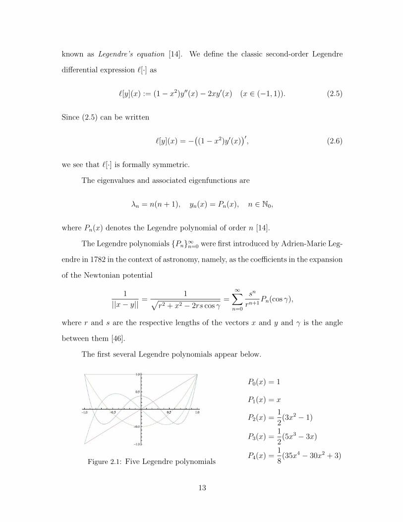
The first several Legendre polynomials appear below.

Figure 2.1: Five Legendre polynomials

P0(x) = 1

P1(x) = x

P2(x) =1

2(3x2 − 1)

P3(x) =1

2(5x3 − 3x)

P4(x) =1

8(35x4 − 30x2 + 3)

13

CHAPTER THREE

The GKN Theory of Self-Adjoint Extensions of Symmetric Operators

3.1 Symmetric Operators

Let H be a complex Hilbert space with inner product (·, ·) and let the operator

T : D(T )→ H be densely defined, i.e., the domain of T , D(T ), is a dense subset of

H. In this setting, we now define the Hilbert-adjoint operator, T ∗, of T . The domain

D(T ∗) consists of all y ∈ H such that the mapping fy := x→ (Tx, y) is continuous

on D(T ). By the Hahn-Banach theorem, fy has a continuous extension to all of H.

Hence, by the Riesz representation theorem, there exists a unique y∗ ∈ H such that

(Tx, y) = (x, y∗) for all x ∈ D(T ). We define T ∗y = y∗.

An operator T is Hermitian if, for all x, y ∈ D(T ) whereD(T ) is not necessarily

dense in H, (Tx, y) = (x, Ty). If in addition to being Hermitian T has a dense

domain, then T is called symmetric. The following theorem, proved by Hellinger

and Toeplitz, shows that an unbounded Hermitian operator T cannot be defined on

all of H.

Theorem 3.1. If a linear operator T is defined on all of a complex Hilbert space H

and satisfies (Tx, y) = (x, Ty) for all x, y ∈ H, then T is bounded.

Proof. See [45].

Because the domain of an unbounded symmetric operator T is a proper sub-

space of H, it makes sense to study symmetric extensions (if they exist) of the

operator T in H. The next theorem gives relationships between the adjoint of a

symmetric operator and the adjoint of its symmetric extension. We write S ⊂ T

when the operator T is an extension of the operator S, meaning that D(S) ⊆ D(T )

and S[f ] = T [f ] for f ∈ D(S).

14

Theorem 3.2. Suppose that T is a densely defined operator on a Hilbert space H.

(i) T is symmetric if and only if T ⊂ T ∗.

(ii) If S is an extension of T , then T ∗ is an extension of S∗, i.e., T ⊂ S implies

S∗ ⊂ T ∗.

(iii) If T is symmetric, then every symmetric extension S of T satisfies

T ⊂ S ⊂ S∗ ⊂ T ∗.

A densely defined operator with the property that T = T ∗ is self-adjoint.

Property (i) of Theorem 3.2 shows that every self-adjoint operator is symmetric, but

the converse is not true; however, in the case of a bounded operator T : H → H,

the concepts of symmetry and self-adjointness are identical. From property (iii) of

Theorem 3.2, we see that the most general symmetric extension in H (in particular,

the most general self-adjoint extension) of a symmetric operator T , is a suitably

chosen restriction of the adjoint T ∗ of T . We characterize the domains of self-adjoint

extensions of a general unbounded operator S below.

3.2 Weyl Theory

Suppose ak : (a, b)→ C is such that ak ∈ Ck(a, b), k = 0, 1, ..., n. Let

L[y] =n∑k=0

aky(k), y ∈ Cn(a, b). (3.1)

The Lagrange adjoint (or formal adjoint) of L[·] is the differential expression

L∗[y] =n∑k=0

(−1)k(aky)(k).

The expression L[·] is formally symmetric if L[y] = L∗[y] for all y ∈ Cn(a, b). Theo-

rem 3.3 determines a general form for all formally symmetric differential operators

with real-valued coefficients.

15

Theorem 3.3. Suppose L[·] is given as in (3.1) with each coefficient ak ∈ Ck(a, b)

being real-valued. If L[·] is formally symmetric, then n is necessarily even and L[·]

may be written as

L[y] =

n/2∑k=0

(−1)k(bky(k))(k).

Proof. See [15].

Since the domain of L consists of all functions y with n derivatives and the

domain of L∗ consists of all functions y such that (aky)(k) exists for k = 0, 1, ..., n,

it follows that D(L) ⊆ D(L∗). Therefore formal symmetry corresponds to the usual

definition of symmetry from the previous section.

Weyl studied the solutions to the Sturm-Liouville differential equation

Dλ[y](x) := [p(x)y′(x)]′ + [λw(x)− q(x)]y(x) = 0 (3.2)

on the interval (a, b) where

(i) p, p′, q and w are real-valued and continuous on (a, b);

(ii) p(x) > 0 and w(x) > 0 in (a, b); and

(iii) λ ∈ C.

Note that if we define

`[y] :=1

w

(− (py′)′ + qy

),

then, by Theorem 3.3, w`[y] is formally symmetric and the equation `[y] = λy is

fully equivalent to Dλy = 0. A solution of (3.2) is a function y ∈ C2(a, b) such that

Dλ[y](x) = 0 for every x ∈ (a, b).

The following two theorems proved by Weyl are essential in extending sym-

metric operators.

16

Theorem 3.4. Let λ0 ∈ C (possibly real) and let x0 ∈ (a, b). Suppose∫ b

x0

|y(x)|2w(x)dx <∞

for all solutions y(x) of Dλ0 [y] = 0. Then∫ b

x0

|v(x)|2w(x)dx <∞

for all solutions v(x) of Dλ[y] = 0 for all λ ∈ C. A similar result holds at the other

endpoint a of (a, b).

Proof. See [32].

Theorem 3.5. Let x0 ∈ (a, b) and let λ ∈ C with Im(λ) 6= 0. Then

(i) there exists at least one solution u(x) 6≡ 0 of Dλ[y] = 0 such that∫ b

x0

|u(x)|2w(x)dx <∞;

(ii) if there exists at least one solution u(x) of Dλ[y] = 0 with∫ b

x0

|u(x)|2w(x)dx =∞,

then for every solution v(x) of Dλ[y] = 0 which satisfies∫ b

x0

|v(x)|2w(x)dx <∞

we have

limx→b

p(x)[v′(x)v(x)− v(x)v′(x)] = 0;

(iii) if ∫ b

x0

|u(x)|2w(x)dx <∞

for every solution u(x) of Dλ[y] = 0 then there exists a fundamental system

u1(x), u2(x) of Dλ[y] = 0 and a circle |ξ− ξ0| = r0 in the complex plane with

center ξ0 and radius r0 > 0 such that for w(x) = ξu1(x) + u2(x), we have

limx→b

p(x)[w′(x)w(x)− w(x)w′(x)] = 0

for all ξ which lie on the circle.

17

Corresponding statements are true at the endpoint a of (a, b).

Proof. See [32].

Weyl’s proof of Theorem 3.5 is geometric and involves a series of contracting

circles, hence, in view of his second theorem, we say that at x = b the limit-circle

case with respect to λ occurs if for λ∫ b

x0

|u(x)|2w(x)dx <∞

for every solution u(x) of Dλ[y] = 0. We say that at x = b the limit point case with

respect to λ occurs if for λ there exists only one linearly independent solution u(x)

of Dλ[y] = 0 for which ∫ b

x0

|u(x)|2w(x)dx =∞

with corresponding terminology at the endpoint a of (a, b). The next theorem, known

as Weyl’s alternative, shows that these definitions are independent of λ.

Theorem 3.6 (Weyl’s Alternative). The occurrence of the limit circle case and the

limit point case, respectively, is independent of λ.

Proof. See [32].

We now discuss the von Neumann-Stone theory of symmetric extensions of

symmetric operators; the standard reference in this case is [15].

3.3 Extensions of General Symmetric Operators

Suppose T : D(T )→ H is a densely defined symmetric operator. Let

D+ = {f ∈ D(T ∗) | T ∗f = if}

and

D− = {f ∈ D(T ∗) | T ∗f = −if}

18

where i =√−1. Then the spaces D+ and D− are respectively called the positive

and negative deficiency spaces of T . We call the dimensions n+ = dimD+ and

n− = dimD− the positive and negative deficiency indices of T .

The graph G(T ) of an operator T is the subset of H⊕H consisting of all points

of the form (x, Tx) with x ∈ D(T ). If G(T ) is a closed subset of H ⊕H in the inner

product defined by

((x1, x2), (y1, y2)

)= (x1, y1) + (x2, y2)

then T is a closed operator. (Equivalently, T is closed if whenever {xn} ⊂ D(T )

satisfies xn → x and Txn → y, then x ∈ D(T ) and Tx = y.) We say that T1 is a

minimal closed linear extension of T if whenever S is a closed linear extension of T ,

we have T1 ⊂ S. In this case we call T1 the closure of T and write T = T1. T is

closable or is said to admit a closure if such a closed linear extension exists. With

regard to self-adjoint operators, we have the following theorem.

Theorem 3.7. Let T : D(T )→ H be a symmetric operator.

(i) T exists (that is, T admits a closure) and is a uniquely defined symmetric

operator.

(ii) The operators T and T have the same closed extensions.

(iii) A self-adjoint operator is closed.

Proof. See [15].

Since we are concerned with self-adjoint extensions of symmetric operators T ,

by the above theorem we can concentrate on the consideration of closed symmetric

extensions of T .

If x, y ∈ D(T ∗), define

(x, y)∗ := (x, y) + (T ∗x, T ∗y).

19

We see then that (x, y)∗ is simply the inner product that D(T ∗) inherits from the

previously defined inner product on H ⊕H if we identify D(T ∗) with G(T ∗) via the

map x → (x, T ∗x). Then it can be verified that D(T ∗) is a complete Hilbert space

under the inner product (x, y)∗. The following theorem gives a decomposition of the

Hilbert space D(T ∗) as a direct sum of closed orthogonal subspaces.

Theorem 3.8. Suppose T : D(T )→ H is a symmetric operator. Then

(i) D(T ), D+, and D− are closed, mutually orthogonal subspaces of D(T ∗) in

the inner product (x, y)∗, and

(ii) D(T ∗) = D(T )⊕D+ ⊕D−.

Proof. See [15].

The representation of D(T ∗) in property (ii) of the above theorem is known as

von Neumann’s formula. Since by Theorem 3.7 every closed symmetric extension S

of a symmetric operator T satisfies T ⊂ S ⊂ S∗ ⊂ T ∗, we see from von Neumann’s

formula that the space D+ ⊕ D− plays a central role in the search for self-adjoint

extensions of the operator T . The theorem and corollary below give us the connection

between this space and the domains of closed symmetric extensions of T .

Theorem 3.9. Let T : D(T ) → H be a symmetric operator. Let G ′ be a closed

subspace of D+ ⊕D− and G = D(T )⊕ G ′.

(i) The space G is the domain of a closed symmetric extension of T if and only

if G ′ is the graph of an isometric transformation mapping a subspace of D+

onto a subspace of D−.

(i) The restriction of T ∗ to G is self-adjoint if and only if G ′ is the graph of an

isometric transformation mapping D+ onto all of D−.

Proof. See [15].

20

Corollary 3.10. (i) A symmetric operator T has self-adjoint extensions if and only

if its deficiency indices n+ and n− are equal.

(ii) If n+ = n− = 0, the only self-adjoint extension of T is its closure T = T ∗.

Proof. This corollary is an immediate consequence of Theorems 3.7, 3.8, and 3.9

and the fact that two Hilbert spaces are isometrically isomorphic if and only if they

have the same dimension [50].

We note that although symmetric operators with unequal deficiency indices

do not have self-adjoint extensions, it is still possible for such operators to have

symmetric extensions (for an example, see [50]).

3.4 Extensions of Symmetric Differential Operators

Let (a, b) be an open interval of R with ∞ ≤ a < b ≤ ∞. In this section,

the Hilbert space H is the Lebesgue space L2(a, b). By Theorem 3.3, every formally

symmetric differential expression L[·] of order 2n with coefficients ak : (a, b) → R

and ak ∈ Ck(a, b) for k = 0, 1, ..., n and n ∈ N is of the form

L[y](x) =n∑k=0

(−1)k(ak(x)y(k)(x)

)(k), x ∈ (a, b). (3.3)

In this section we assume that

1

an, an−1, ..., a1, a0 ∈ Lloc(a, b).

The endpoint a is a regular point of L[·] and L[·] is regular at a if a > −∞ and there

exists an ε > 0 such that

1

an, an−1, ..., a1, a0 ∈ Lloc(a, a+ ε).

Otherwise the endpoint a is a singular point of L[·] and L[·] is singular at a. We use

similar terminology at the endpoint b. The expression L[·] is said to be regular if both

a and b are regular points, otherwise L[·] is singular. Since the Legendre operator is

21

a singular expression in (−1, 1), we assume here that L[·] is singular though much of

the theory applies equally well to the regular case, as described in Naimark (see [52]).

We note here that Naimark considers symmetric differential expressions with fewer

differentiability requirements. Indeed, the less restrictive hypotheses assumed by

Naimark and other authors lead them to the concept of the quasi-derivative, which

we define below in the context of defining the sesquilinear form. However, since the

coefficients of the Legendre expression are polynomials, we assume as above that

ak ∈ Ck(a, b).

The maximal operator L generated by the expression L[·] is defined by

L[y] := L[y]

D(L) := {y : (a, b)→ C | y(k) ∈ ACloc(a, b), k = 0, 1, ..., 2n− 1;

y, L[y] ∈ L2(a, b)},

(3.4)

where L[·] is given by (3.3). Note that the term “maximal” is appropriate because

the space D(L) is the largest possible subspace for which L can be defined as an

operator from L2(a, b) into L2(a, b).

For ease of notation in the definition of the sesquilinear form below, we now

define the concept of the quasi-derivative. The kth quasi-derivative y[k] of a function

y is defined as

y[0] = y = y(0)

y[k] = y(k), k = 0, 1, ..., n− 1

y[n] = any(n)

y[n+k] = an−ky(n−k) −

[y[n+k−1]

]′, k = 1, 2, ..., n− 1

where, as above,

1

an, an−1, ..., a1, a0 ∈ Lloc(a, b)

and y(k) denotes the usual derivative. Using the quasi-derivative, we define the

22

sesquilinear (symplectic) form [y, z](·) of two functions y and z by

[y, z] =n∑k=1

{y[k−1]z[2n−k] − y[2n−k]z[k−1]

}(3.5)

where z denotes the usual complex conjugate of z and y[k] denotes the kth quasi-

derivative of y. We note that without using quasi-derivatives, the sesquilinear form

takes the form

[y, z] =n∑k=1

k∑j=1

(−1)k+j{

(akz(k))(k−j)y(j−1) − (aky

(k))(k−j)z(j−1)}.

For f, g ∈ D(L) and any compact subinterval [α, β] ⊂ (a, b), the following

formula can be easily verified by integration by parts:∫ β

α

{`[f ]g − `[g]f} dx = [f, g](x)∣∣βα, (3.6)

where [f, g](·) is the sesquilinear form defined in (3.5). Notice that for all f, g ∈ D(L)

and a < x < b, [g, f ](x) = −[f, g](x). By the definition of D(L) and Holder’s

inequality, we have the following theorem.

Theorem 3.11. The limits

[f, g](b) := limx→b−

[f, g](x) and [f, g](a) := limx→a+

[f, g](x)

both exist and are finite for all f, g ∈ D(L).

Proof. See [52].

Equation (3.6) is known as Green’s formula for L[·], which is essential in the

determination of all self-adjoint extensions in L2(a, b) of the minimal operator gen-

erated by L[·], which we now discuss.

Define a restriction L′0 of the maximal operator L by

L′0[y] := L[y]

D(L′0) := {y ∈ D(L) | y has compact support in (a, b)}.

23

For reasons that will soon become clear, we call L′0 the pre-minimal operator. It can

be shown that the operator L′0 is symmetric (see [52]). Hence, by Theorem 3.7, L′0

admits a closure in L2(a, b) which is also symmetric. Let

L0 := L′0.

Then L0 is called the minimal operator generated by L[·]. Since D(L0) is dense in

L2(a, b), the adjoint operator L0 exists. The following theorem states the relationship

between the maximal operator L and the minimal operator L0.

Theorem 3.12. L∗0 = L and L∗ = L0.

Proof. See [52].

In general, if a densely defined operator has a “large” domain, its adjoint will

have a “small” domain, as described in property (ii) of Theorem 3.2. Therefore,

since the maximal operator has the largest possible domain, its adjoint (the minimal

operator) has the minimally small domain. Since L and L0 have the same form as the

operator L, we call the operator with the maximal domain the maximal operator L

and the operator with the minimal domain the minimal operator L0. It follows that

to find self-adjoint operators generated by L[·], we need to either look at extensions

of D(L0) or restrictions of D(L).

To determine whether a function f ∈ D(L) is in the minimal domain D(L0),

we have the following theorem which makes use of the sesquilinear form.

Theorem 3.13. The minimal domain, i.e., the domain of the minimal operator L0,

is given by

D(L0) = {f ∈ D(L) | [f, g](x)∣∣ba

= 0 for all g ∈ D(L)}.

Proof. See [52].

24

From Corollary 3.10 and the following theorem, due to the equality of the

positive and negative deficiency indices of L0, the minimal operator does have self-

adjoint extensions in L2(a, b).

Theorem 3.14. The deficiency indices of the operator L0 have the form (m,m) where

0 ≤ m ≤ 2n (and 2n is the order of the differential expression L[·]).

Proof. See [52].

In fact, as shown by Glazman by means of actual examples, m can take on

each value between 0 and 2n. On a side note, in the case of an operator L[·] with

one singular endpoint and one regular endpoint, the range of the deficiency indices

is limited to n ≤ m ≤ 2n [52].

In Section 3.2 above we defined the terms limit-point and limit-circle for

second-order formally symmetric differential expressions. We generalize this ter-

minology to a differential operator L[·] or order 2n by using the term limit-m at the

endpoint a if there exist exactly m linearly independent solutions to L[y] = λ[y] that

belong to L2(a, x0) for some x0 ∈ (a, b). In particular, if n = 1, the original terms

limit-point and limit-circle apply in place of limit-1 and limit-2.

3.5 Glazman-Krein-Naimark (GKN) Theory

We turn now to the calculation of the deficiency indices for the operator L0

when there are two singular endpoints, which is the case for the Legendre differential

operator at ±1.

Before stating the GKN theorem, we introduce the following definition.

Definition 3.15. Suppose M1 and M2 are subspaces of a vector space V such that

M1 ⊂M2. Let {x1, x2, ..., xn} ⊆M2. We say that {x1, x2, ..., xn} is linearly indepen-

dent modulo M1 if

n∑i=1

αixi ∈M1 implies αi = 0, i = 1, 2, ..., n.

25

The dimension of M2 modulo M1 is the maximum number of vectors in M2 that are

linearly independent modulo M1. If this dimension is n ≤ ∞, then we write that

dim M2 = n mod (dim M1).

The following theorem characterizes all self-adjoint extensions of L0.

Theorem 3.16 (GKN). Suppose the deficiency indicies of L0 are n+ = n− := m.

(i) Let S be a self-adjoint extension of L0 (in L2(a, b)). Then there exist

w1, w2, ..., wm ∈ D(S) such that {w1, w2, ..., wm} is a set which is linearly

independent modulo D(L0) where

(a) Sx = Lx = Lx;

(b) D(S) = {x ∈ D(L) | [x,wj]∣∣ba

= 0, j = 1, 2, ...,m}; and

(c) [wi, wj]∣∣ba

= 0 for i, j = 1, 2, ...,m. (These are called Glazman symmetry

conditions.)

(ii) Conversely, suppose {w1, w2, ..., wm} ⊆ D(L) are such that they are linearly

independent modulo D(L0) and satisfy the Glazman symmetry conditions

in (c) above. Then with S as defined in (a) and (b), S is a self-adjoint

extension of L0.

Proof. See [52].

In chapter five, we use the GKN theorem (3.16) to find all self-adjoint exten-

sions of the minimal operator associated with the Legendre differential expression

below, and then find the particular self-adjoint extension which has the Legendre

polynomials as eigenfunctions.

3.6 The Method of Frobenius

In this section we describe the method of Frobenius, which is a technique for

finding n linearly independent solutions in the form of generalized power series for

26

certain types of ordinary differential equations of order n. We use this method to

determine whether a Sturm-Liouville expression (3.2) is limit-point or limit-circle,

which then determines the deficiency indices of the expression. The method of

Frobenius can be generalized for a higher order differential equation up to limit-2n

as discussed above.

Consider the differential equation given by

M [y](z) := a2(z)y′′(z) + a1(z)y′(z) + a0(z)y(z) = 0 (3.7)

where each ak, k = 0, 1, 2, is analytic in some open neighborhood N(a) of a ∈ C.

We say that z = a is a regular point of M [·] if a2(a) 6= 0. The point z = a is a

regular singular point of M [·] if

ak(z)

a2(z)has a pole of order ≤ 2− k at z = a (k = 0, 1),

otherwise, z = a is called an irregular singular point of M [·].

If z = a is a regular singular point of M [·], then

Pk(z) =(z − a)2−kak(z)

a2(z)(k = 0, 1)

is analytic in N(a). Then (3.7) may be rewritten as

M [y](z) =a2(z)

(z − a)2[(z − a)2y′′(z) + (z − a)P1(z)y′(z) + P0(z)y(z)].

The expression

(z − a)2y′′(z) + (z − a)P1(z)y′(z) + P0(z)y(z) (3.8)

is called the canonical form of M [y](z).

The method of Frobenius shows that (3.8) always has a solution of the form

y1(z) =∞∑k=0

ak(z − a)k+r1

27

for some value r1 ∈ C. In fact, r = r1 is a root of the indicial equation, which is

given by

r(r − 1) + rP1(a) + P0(a) = 0. (3.9)

The following is a precise statement of the method of Frobenius for second-order

differential equations.

Theorem 3.17. Consider the second-order differential equation (3.8) and suppose

r = r1 and r = r2 are the roots of the indicial equation (3.9) with Re(r1) ≥ Re(r2).

(i) If r1 − r2 6∈ N0, then (3.8) has a basis of solutions {y1, y2} of the form

y1(x) =∞∑n=0

an(r1)(x− a)n+r1 (a0(r1) 6= 0)

y2(x) =∞∑n=0

bn(r2)(x− a)n+r2 (b0(r2) 6= 0).

(ii) If r1 = r2, then (3.8) has a basis of solutions {y1, y2} of the form

y1(x) =∞∑n=0

an(r1)(x− a)n+r1 (a0(r1) 6= 0)

y2(x) = log(x− a)y1(x) +∞∑n=0

bn(r2)(x− a)n+r2 (b0(r2) 6= 0).

(iii) If r1 − r2 ∈ N, then (3.8) has a basis of solutions {y1, y2} of the form

y1(x) =∞∑n=0

an(r1)(x− a)n+r1 (a0(r1) 6= 0)

y2(x) = k log(x− a)y1(x) +∞∑n=0

bn(r2)(x− a)n+r2 (b0(r2) 6= 0)

for some k ∈ C.

Note that if the roots of the indicial equation involve a parameter, all possible

values of the parameter must be considered in order to determine the form of the

basis of solutions [62]. For further details of the method described above, see the

appendix of [50].

28

CHAPTER FOUR

Properties and Restrictions of the Maximal Domain

In this chapter we study the Legendre differential expression

`[y](x) := (1− x2)y′′(x)− 2xy′(x) + ky(x)

= −((1− x2)y′(x)

)′+ ky(x) (x ∈ (−1, 1)),

(4.1)

where k ≥ 0 is a fixed constant. Note that k = 0 in the original definition of

Legendre’s equation as written in (2.5). As we will see below, for the spectral

analysis of the Legendre operator, it is essential to have k > 0.

The classical Legendre polynomials satisfy the second-order differential equa-

tion

`[y] = (λn + k)y, (4.2)

where λn = n(n+1), and hence, they are eigenfunctions of `[·] as defined in (4.1). An

explicit formula for these polynomials is given in (2.2). The Legendre polynomials

are orthogonal in the space L2(−1, 1) with explicit orthogonality relationship given

in (2.3). We investigate the self-adjoint operator in L2(−1, 1) having the Legendre

polynomials as eigenfunctions, which we refer to as the “Legendre polynomials op-

erator.” The original study of the Legendre differential equation in the right-definite

case is due to Titchmarsh (see [64]) who began his investigation in 1941. Early in

the 1950s, Glazman analyzed the right-definite problem using an operator approach.

We also study the operator `[·] in the Hilbert space H21 (−1, 1) defined by

H21 (−1, 1) := {f : (−1, 1)→ C | f ∈ ACloc(−1, 1); f, (1− x2)

12f ′ ∈ L2(−1, 1)}

with inner product

(f, g)1 :=

∫ 1

−1

{(1− x2)f ′(x)g′(x) + kf(x)g(x)

}dx,

29

which is the left-definite boundary problem. As a consequence, we establish the

orthogonality relationship

(Pn, Pm)1 =(n(n+ 1) + k

) 2

2n+ 1δnm. (4.3)

In 1980, Everitt [19] published a study of the right- and left-definite problems

for the Legendre differential equation which utilizes the theory found in Titchmarsh

[64]. The work of Everitt has been extended by Onyango-Otieno [54], who used the

Titchmarsh approach to study the right- and left-definite problems for the classical

differential equations of Jacobi, Laguerre, and Hermite.

4.1 Properties of the Maximal Domain of `[·]

The maximal domain ∆1,max of `[·] in L2(−1, 1) is defined to be

∆1,max := {f : (−1, 1)→ C | f, f ′ ∈ ACloc(−1, 1); f, `[f ] ∈ L2(−1, 1)}. (4.4)

Since C∞0 ⊂ ∆1,max, it follows that ∆1,max is dense in L2(−1, 1).

For f, g ∈ ∆1,max and [a, b] ⊂ (−1, 1), we have (as in (3.6)) Green’s formula∫ b

a

{`[f ](x)g(x)− f(x)`[g](x)} dx = [f, g]1(x)

∣∣∣∣ba

where [f, g]1(·) is the skew-symmetric sesquilinear form defined by

[f, g]1(x) := −(1− x2)[f ′(x)g(x)− g′(x)f(x)] (4.5)

and Dirichlet’s formula∫ b

a

{(1− x2)f ′(x)g′(x) + kf(x)g(x)

}dx = (1− x2)f ′(x)g(x)

∣∣∣∣ba

+

∫ b

a

`[f ](x)g(x)dx.

(4.6)

Note that by definition of ∆1,max, the limits as x → ±1 of [f, g](x) exist and are

finite for all functions f, g ∈ ∆1,max.

To find the deficiency indices n+ and n− of `[·], we solve

`[y](x) = −((1− x2)y′(x)

)′= 0,

30

since by Weyl’s Alternative (see 3.6), the occurrence of the limit-point and limit-

circle case is independent of k in

`[y] = ky. (4.7)

We note that y1(x) = 1 is a solution. To find y2, we set

y′2(x) =1

1− x2

and use the method of partial fractions to integrate and find that

y2(x) =1

2log

1 + x

1− x.

Noting that both y1 and y2 are L2 near x = ±1, we see that `[y] has two L2 solutions

near each endpoint, and since `[y] is a second-order differential equation, we calculate

the deficiency index to be (2, 2) [68].

On the other hand, since both ±1 are regular singular endpoints of (2.4),

we can also use the method of Frobenius to give the general form of two linearly

independent solutions of

`[y] = 0. (4.8)

Although the Frobenius solutions are superfluous in this case since we already solved

(4.7), we list them because in later chapters we will be working with powers of the

Legendre differential expression which necessarily have higher orders, where it will

not be possible to find explicit solutions to the analogous differential equations. The

indicial equation of (4.8) is r2 = 0, therefore the Frobenius solutions to (4.8) are of

the form

y1(x) =∞∑n=0

an(x− 1)n, a0 6= 0

and

y2(x) = log |1− x|∞∑n=0

an(x− 1)n +∞∑n=0

bn(x− 1)n, b0 6= 0, (4.9)

31

where all the series converge for |x− 1| < 2. There exist corresponding solutions at

the regular singular endpoint x = −1.

We now list the properties of the maximal domain ∆1,max.

Theorem 4.1. Let f, g ∈ ∆1,max. Then

(i) 1 ∈ ∆1,max and limx→±1

[f, 1](x) = limx→±1

−(1− x2)f ′(x).

(ii) If h± ∈ C2(−1, 1) are defined by

h+(x) =

−12

log(1− x2) for x near 1

0 for x near − 1

and

h−(x) =

0 for x near 1

12

log(1− x2) for x near − 1,

then h± ∈ ∆1,max. Furthermore,

limx→+1

[f, h+](x) = limx→+1

{1

2(1− x2) log(1− x2)f ′(x) + xf(x)

}and

limx→−1

[f, h−](x) = limx→−1

{−1

2(1− x2) log(1− x2)f ′(x)− xf(x)

}.

(iii) limx→±1

[f, g](x) = limx→±1

{[f, 1](x)g(x)− [g, 1](x)f(x)} .

Proof. This theorem is an immediate consequence of definition (4.5).

We remark that the above theorem is as strong as possible in the sense that

the solution y2, given in (4.9), of (4.8) is in ∆1,max but limx→±1

y2(x) do not exist.

We next consider properties of a restriction D1 of ∆1,max and then show that

D1 is the domain of the self-adjoint operator in L2(−1, 1) having the Legendre poly-

nomials as a complete set of orthogonal eigenfunctions.

32

4.2 Properties of a Restriction of the Maximal Domain

Define, for f ∈ ∆1,max and x ∈ (−1, 1),

Λ[f ](x) :=

∫ x

0

{`[f ](t)− kf(t)} dt− f ′(0) = −(1− x2)f ′(x). (4.10)

By definition of ∆1,max, given in (4.4),

Λ′[f ] ∈ L2(−1, 1) (4.11)

whenever f ∈ ∆1,max. Hence, by defining Λ[f ](±1) := limx→±1

Λ[f ](x), we have then

that Λ[f ] ∈ AC[−1, 1].

Let e± ∈ C2[−1, 1] have the properties

e+(x) =

1 for x near 1

0 for x near − 1

and

e−(x) =

0 for x near 1

1 for x near − 1.

Note that e± ∈ ∆1,max. Define a restriction D1 of ∆1,max by

D1 := {f ∈ ∆1,max | [f, e+](1) = [f, e−](−1) = 0}. (4.12)

An important characterization of D1 is given in the next lemma.

Lemma 4.2. Let f ∈ ∆1,max. Then f ∈ D1 if and only if Λ[f ](±1) = 0.

Proof. By property (i) of the theorem above and by the definition of Λ[·], we have

the identities [f, e+](1) = Λ[f ](1) and [f, e−](−1) = Λ[f ](−1) whenever f ∈ ∆1,max.

This lemma is now a direct consequence of the definition of D1 given in (4.12).

The next theorem lists properties of functions in D1.

33

Theorem 4.3. Let f, g ∈ D1. Then

(i) f ′ ∈ L2(−1, 1);

(ii) f ∈ AC[−1, 1];

(iii) limx→±1

(1− x2)f ′(x)g(x) = 0; and

(iv) limx→±1

[f, g](x) = 0.

Proof. Property (i) of this theorem was first proved in 1988 by Everitt and Maric [27].

We give their proof of this property below.

Let f ∈ D1. Then Λ[f ](1) = 0 by the lemma above. Furthermore, by (4.11),

Λ′[f ] ∈ L2(−1, 1). Hence, using the definition of Λ[·] in (4.10), we have the repre-

sentation

f ′(x) = − Λ[f ](x)

(1− x2)=

1

1− x2

∫ 1

x

Λ′[f ](t)dt

for x ∈ [0, 1). Since ∫ x

0

1

(1− t2)2dt

∫ 1

x

12dt ≤ K

for some constant K > 0 and for all x ∈ [0, 1), we have f ′ ∈ L2[0, 1) by the CE

Theorem [12]. (A statement of the CE Theorem can be found in Section 7.3.)

Similarly, f ′ ∈ L2(−1, 0] and property (i) is proved.

Property (ii) is now an immediate consequence of property (i).

Assume f, g ∈ D1. From property (i) of this theorem and Holder’s inequality,

we see that (1 − x2)f ′(x)g′(x) ∈ L(−1, 1). Hence, we can now see from Dirichlet’s

formula (4.6) that limx→±1

(1− x2)f ′(x)g(x) exist and are finite. If, for instance,

(1− x2)|f ′(x)g(x)| ≥ c

for x near 1, then |f ′(x)g(x)| ≥ c

1− x2when x is close to 1. This would indicate

that |f ′(x)g(x)| 6∈ L2(−1, 1). Therefore, it must be the case that limx→+1

f ′(x)g(x) = 0.

Similarly, limx→−1

(1− x2)f ′(x)g(x) = 0. Thus, property (iii) is proved. Property (iv)

34

follows from property (iii) and the definition of the sesquilinear form [·, ·] given in

(4.5).

We note that D1 is a proper subspace of ∆1,max. For example, the solu-

tion y2 given in (4.8) of (4.9) is an element of ∆1,max which is not in D1. Fur-

thermore, property (i) of this theorem is as strong as possible in the sense that

f(x) =

∫ x

0

log(1− t2)dt, x ∈ (−1, 1) is in D1 but f ′′ 6∈ L2(−1, 1).

In 2001, Everitt, Littlejohn, and Maric extended Theorem 4.3 to include even

more equivalent conditions. We discuss this below in Section 5.3 (see Theorem 5.6).

4.3 The Right-Definite Problem

The spaceD1 studied in the above section has the property thatD1 ⊂ L2(−1, 1);

hence, we can define an operator T1 in L2(−1, 1) by

T1[f ](x) := `[f ](x), x ∈ (−1, 1)

D(T1) := D1

Theorem 4.4. T1 is self-adjoint in L2(−1, 1).

Proof. From (3.13), the minimal domain of the differential expression `[·] in L2(−1, 1)

is

Dmin(T1) =

{y ∈ ∆1,max

∣∣∣∣[y, z]∣∣∣∣1−1

= 0 for all z ∈ ∆1,max

}.

Now if the linear combination α+e+ + α−e− for α± ∈ C of the functions e± defined

at the beginning of the previous section is in Dmin(T1), then

0 = [α+e+ + α−e−, h+](1) = α+

and

0 = [α+e+ + α−e−, h−](−1) = α−,

where h± ∈ ∆1,max are the functions defined in property (ii) of the Theorem 4.1.

Therefore, e± are linearly independent modulo Dmin(T1). The functions e± also

35

satisfy the Glazman symmetry conditions from the GKN Theorem by property (i)

of Theorem 4.1. Hence, by the GKN Theorem, T1 is self-adjoint in L2(−1, 1).

If f, g ∈ D(T1) = D1, then by Dirichlet’s formula (4.6) and property (iii) of

the previous theorem,

(T1[f ], g) =

∫ 1

−1`[f ](t)g(t)dt =

∫ 1

−1

{(1− t2)f ′(t)g′(t) + kf(t)g(t)

}dt. (4.13)

Hence, if we let f = g, equation (4.13) becomes

(T1[f ], f) =

∫ 1

−1

{(1− t2)|f ′(t)|2 + k|f(t)|2

}dt

=

∫ 1

−1(1− t2)|f ′(t)|2dt+ k(f, f)

≥ k(f, f).

(4.14)

The inequality in (4.14) holds because (1 − x2)|f ′(x)|2 ≥ 0 for x ∈ (−1, 1). Since

(4.14) is valid for all f ∈ D(T1), we conclude that T1[·] is bounded below by kI in

L2(−1, 1).

Because T1 is bounded below by kI, the number 0 ∈ ρ(T1), the resolvent set

of T1, as long as k > 0. Consequently, the resolvent operator R0(T1) exists and

is a bounded operator from L2(−1, 1) onto D1. We will utilize this operator when

considering the left-definite problem in the next section.

The next theorem completely characterizes the spectrum of T1, with proof

based on the previous theorem.

Theorem 4.5. (i) The Legendre polynomials {Pn}∞n=0 are a complete set of orthogonal

eigenfunctions for the operator T1 in L2(−1, 1).

(ii) The spectrum of T1 in L2(−1, 1) is given by

σ(T1) = {n(n+ 1) + k | n ∈ N},

i.e., T1 has a discrete spectrum which is bounded below and all eigenvalues

are simple.

36

Proof. By construction, the Legendre polynomials are eigenfunctions of T1[·] with

corresponding eigenvalues {n(n+1)+k | n ∈ N} as above. Furthermore, by Theorem

2.4, {Pn}∞n=0 is a complete orthogonal polynomial sequence in L2(−1, 1).

We proved in Theorem 4.4 that the operator T1 is self-adjoint, therefore its

residual spectrum is empty. Since the set of eigenvalues of T1, {n(n+1)+k | n ∈ N},

has no finite accumulation points, it follows that the continuous spectrum of T1 is

also empty (see [57]). Hence the spectrum of T1 contains only the eigenvalues of T1,

so the statement in part (ii) of the theorem follows.

In the next chapter, we discuss the properties of A, the particular self-adjoint

operator that has the Legendre polynomials as eigenfunctions.

37

CHAPTER FIVE

The Legendre Polynomials Self-Adjoint Operator A

In this chapter, we show how the GKN theorem can be applied to the Legen-

dre expression `[·] to produce all of the self-adjoint extensions in L2(−1, 1) of the

associated minimal operator, including that extension having the Legendre polyno-

mials as a complete set of eigenfunctions. We note that in this classical second-order

case, the symmetry factor f for the expression is identical with the orthogonalizing

weight function (which in the Legendre case is w(x) = 1) for the associated or-

thogonal polynomials, the Legendre polynomials {Pn}∞n=0. Consequently, the GKN

theory of self-adjoint extensions of the minimal operator L0 will yield, as a special

case, that self-adjoint extension having the corresponding orthogonal polynomials

as eigenfunctions [23].

In Section 4.1, we found the solutions y1 and y2 for (4.7) and calculated the

deficiency indices to be (2, 2). By von Neumann’s formula (see (3.8)), we have that

dim(D+ ⊕D−) = 4. By the first isomorphism theorem from algebra,

D(L)/D(L0) ∼= D+ ⊕D−. (5.1)

We now construct a basis for the space (5.1). Define {ϕ1, ϕ2, ϕ3, ϕ4} ⊆ D(L) by

ϕ1(x) =

0 near x = −1

1 near x = 1,

ϕ2(x) =

1 near x = −1

0 near x = 1,

ϕ3(x) =

0 near x = −1

12

log 1+x1−x near x = 1

,

38

ϕ4(x) =

12

log 1+x1−x near x = −1

0 near x = 1.

To show that the set {ϕ1, ϕ2, ϕ3, ϕ4} is linearly independent modulo D(L0), suppose

that4∑

k=1

αkϕk ∈ D(L0).

We want to show that α1 = α2 = α3 = α4 = 0. By definition, we have that

y ∈ D(L0) if and only if [y, z]∣∣1−1 = [y, z](1)− [y, z](−1) = 0 for all z ∈ D(L). Hence

4∑k=1

αk[ϕk, ϕi]∣∣1−1 = 0 for i = 1, 2, 3, 4. (5.2)

In the case of the Legendre differential equation, we calculate the sesquilinear form

(3.5) to be

[y, z](x) = (1− x2)(y(x)z′(x)− y′(x)z(x)

).

From the definition of the ϕk, we immediately see that

[ϕ1, ϕ2]∣∣1−1 = [ϕ3, ϕ4]

∣∣1−1 = [ϕ1, ϕ4]

∣∣1−1 = [ϕ2, ϕ3]

∣∣1−1 = 0.

Additionally,

[ϕ1, ϕ3](1) = limx→1

(1− x2)(ϕ1ϕ′3 − ϕ′1ϕ3) = lim

x→1(1− x2)

(1

1− x2− 0

)= 1.

Since both ϕ1 and ϕ3 vanish near −1, [ϕ1, ϕ3](−1) = 0. Hence [ϕ1, ϕ3]∣∣1−1 = 1.

Let i = 1 in (5.2). Since [y, z](x) = −[z, y](x),

0 =���

�����:0

α1[ϕ1, ϕ1]∣∣1−1 +

������

��:0α2[ϕ2, ϕ1]

∣∣1−1 + α3[ϕ3, ϕ1]

∣∣1−1 +

������

��:0α4[ϕ4, ϕ1]

∣∣1−1 = −α3,

hence α3 = 0. Similarly, we determine that α1 = α2 = α4 = 0 and conclude that

{ϕ1, ϕ2, ϕ3, ϕ4} is linearly independent modulo D(L0), i.e., {ϕ1, ϕ2, ϕ3, ϕ4} is a basis

for D(L)/D(L0). Referring back to the GKN theorem (3.16), this means that our

boundary conditions w1 and w2 can be written as

w1 =4∑i=1

ciϕi where (c1, c2, c3, c4) ∈ C4, (5.3)

39

w2 =4∑i=1

kiϕi where (k1, k2, k3, k4) ∈ C4. (5.4)

These two functions must satisfy the Glazman symmetry conditions (as given in (i)

(c) of (3.16))

[w1, w1]∣∣1−1 = [w1, w2]

∣∣1−1 = [w2, w1]

∣∣1−1 = [w2, w2]

∣∣1−1 = 0,

giving us the system of equations

c1c3 − c1c3 − c2c4 + c2c4 = 0

c1k3 − k1c3 − c2k4 + k2c4 = 0

c3k1 − k3c1 − c4k2 + k4c2 = 0

k1k3 − k1k3 − k2k4 + k2k4 = 0.

(5.5)

Hence, every self-adjoint operator S in L2(−1, 1) generated by the Legendre operator

`[y](x) = −((1− x2)y′(x)

)′has the form

Sy = `[y]

D(S) = {y ∈ D(L) | [y, wi]∣∣1−1 = 0, i = 1, 2},

where w1 and w2 are defined in (5.3) and (5.4) and satisfy the conditions listed in

(5.5).

We now focus our attention on determining the self-adjoint extension(s) S

of `[·] in L2(−1, 1) that have the Legendre polynomials {Pn}∞n=0 as eigenfunctions.

Notice that if S is such an extension, then we must necessarily have

[wi, P0]∣∣1−1 = 0, i = 1, 2,

where w1 and w2 are given by (5.3) and (5.4). Since P0(x) ≡ 1, these conditions

yield c3 = c4 and k3 = k4. In addition, since P1(x) = x, we must also have

[wi, x]∣∣1−1 = 0, i = 1, 2,

40

which yields c3 = −c4 and k3 = −k4, forcing c3 = c4 = k3 = k4 = 0. Therefore,

w1 = c1ϕ1 + c2ϕ2 =

c2 near x = −1

c1 near x = 1,

w2 = k1ϕ1 + k2ϕ2 =

k2 near x = −1

k1 near x = 1

where (c1, c2) and (k1, k2) are linearly independent vectors in C2. However, it is easy

to see that

[w1, y]∣∣1−1 = c1[1, y](1)− c2[1, y](−1)

[w2, y]∣∣1−1 = k1[1, y](1)− k2[1, y](−1)

for all y ∈ D(S). From these conditions, it is clear that [y, wi]∣∣1−1 = 0 for i = 1, 2 if

and only if [y, 1](1) = [y, 1](−1) = 0. Consequently, we have the following theorem.

Theorem 5.1. The self-adjoint operator S in L2(−1, 1) which extends the minimal op-

erator L0 generated by the Legendre differential expression `[y] and has the Legendre

polynomials as eigenfunctions is given by

S[y] = `[y]

D(S) = {y ∈ D(L) | [y, 1](1) = [y, 1](−1) = 0}.

Furthermore, the spectrum of S is

σ(S) = {n(n+ 1) + k | n ∈ N0}.

Proof. Details about the spectrum can be found in [50].

Note that by the definition of the sesquilinear form in (4.5), we have that

[1, y](1) = limx→1

(1− x2)y′(x) = 0

[1, y](−1) = limx→−1

(1− x2)y′(x) = 0,

41

hence the operator S given by the GKN theorem is the desired Legendre polynomials

operator A : D(A) ⊂ L2(−1, 1)→ L2(−1, 1), which we define by

Af(x) : = `[f ](x) (a.e. x ∈ (−1, 1))

f ∈ D(A)

(5.6)

where

D(A) : = {f : (−1, 1)→ C | f, f ′ ∈ ACloc(−1, 1); f, `[f ] ∈ L2(−1, 1);

limx→±1

(1− x2)f ′(x) = 0}

= {f ∈ ∆1,max | limx→±1

(1− x2)f ′(x) = 0}.

(5.7)

We now turn to the study of this operator in the appropriately defined right- and

left-definite spaces.

5.1 Hilbert Function Spaces

The two Hilbert function spaces involved in this study of the Legendre differ-

ential expression are

(i) the right-definite space L2(−1, 1), and

(ii) the left-definite space H21 (−1, 1).

The space L2(−1, 1) is the classic integrable-square space of equivalence classes

of Lebesgue measurable functions f : (−1, 1)→ C such that

∫ 1

−1|f(x)|2dx <∞ with

inner product

(f, g) :=

∫ 1

−1f(x)g(x)dx (f, g ∈ L2(−1, 1)).

The space H21 (−1, 1) is defined by

H21 (−1, 1) := {f : (−1, 1)→ C | f ∈ ACloc(−1, 1); (1− x2)

12f ′ ∈ L2(−1, 1)} (5.8)

with inner product

(f, g)1 :=

∫ 1

−1{(1− x2)f ′(x)g′(x) + kf(x)g(x)}dx, (5.9)

42

where k > 0 is the constant given in the definition of `[·] in (2.6). We note that the

definition of H21 (−1, 1) may be simplified to read

H21 (−1, 1) = {f : (−1, 1)→ C | f ∈ ACloc(−1, 1); (1− x2)

12f ′ ∈ L2(−1, 1)}. (5.10)

Indeed, if f ∈ ACloc(−1, 1) and (1− x2) 12f ′ = g ∈ L2(−1, 1), then

f(x) = f(x) +

∫ x

0

g(t)

(1− t2) 12

dt (x ∈ [0, 1));

an application of Holder’s inequality now gives

|f(x)|2 ≤ K| log(1− x)| as x→ 1−

for some K > 0; hence f ∈ L2(0, 1). Similarly f ∈ L2(−1, 0) and so f ∈ L2(−1, 1).

The space H21 (−1, 1) is actually a Hilbert space of functions rather than a

space of equivalence classes as in L2(−1, 1); the null element of H21 (−1, 1) is the zero

function on (−1, 1). The proof that the vector space H21 (−1, 1) is complete in the

norm derived from the inner product (5.9) is given in [50] and [6].

It is well known (see [63]) that the set of Legendre polynomials {Pn}∞n=0 is a

complete, orthogonal set in L2(−1, 1). In fact, the Legendre polynomials also form a

complete orthogonal set in H12 (−1, 1) (see [50] and [6] for proof). It can be seen that

the Legendre polynomials {Pn}∞n=0 are orthogonal in H21 (−1, 1) through well-known

properties of the first derivative of the Gegenbauer polynomials {P (1,1)n }∞n=0; see [63].

Indeed, as we found above, we have the orthogonality relationship (4.3).

See [24] for the proof of the following

Lemma 5.2. For all λ ∈ C, the following properties hold for the solution base

{y1,+(·, λ), y2,+(·, λ)}

of the Legendre differential equation (2.6):

y1,+(·, λ) ∈ L2(0, 1) y2,+(·, λ) ∈ L2(0, 1)

y1,+(·, λ) ∈ H21 (0, 1) y2,+(·, λ) 6∈ H2

1 (0, 1).

43

There are corresponding results for the solution base {y1,−(·, λ), y2,−(·, λ)} and the

spaces L2(−1, 0) and H21 (−1, 0).

5.2 The Legendre Differential Operator A in L2(−1, 1)

This section is based on the general GKN theory of self-adjoint differential

operators generated by real, Lagrange symmetric (formally self-adjoint) differential

expressions in Hilbert spaces; see [52]. Applications of this theory to the classical

second-order differential equations having orthogonal polynomial solutions can be

found, for example, in the theses of Loveland [50] and Onyango-Otieno [54].

The maximal operator T1,max : ∆1,max ⊂ L2(−1, 1) → L2(−1, 1) generated by

the differential expression `[·], given in (2.6), is defined by

∆1,max := {f : (−1, 1)→ C | f, f ′ ∈ ACloc(−1, 1); f, `[f ] ∈ L2(−1, 1)} (5.11)

and

T1,maxf = `[f ] (f ∈ ∆1,max).

The Green’s formula (3.6) shows that the limits

[f, g](−1) := limx→−1+

[f, g](x) and [f, g](1) := limx→1−

[f, g](x)

both exist and are finite for all f, g ∈ ∆1,max.

The minimal operator T1,min : D(T1,min) ⊂ L2(−1, 1) → L2(−1, 1) is then

defined by

D(T1,min) := {f ∈ ∆1,max | [f, g]1(x)∣∣βα

= 0 for all g ∈ ∆1,max}

and

T1,minf = `[f ] (f ∈ D(T1,min)).

From [52], it is known that these linear differential operators have the properties:

(i) T1,min is closed and symmetric in L2(−1, 1);

44

(ii) T ∗1,min = T1,max and T ∗1,max = T1,min so that T1,max is closed in L2(−1, 1);

(iii) the deficiency indices (n+, n−) of T1,min are (2, 2).

Properties (i) and (ii) follow from the general theory; property (iii) follows

from the result that the differential expression `[·] is in the limit-circle condition in

L2(−1, 1) at both endpoints±1 of the interval (−1, 1); in turn this result follows from

the properties in L2(−1, 1) of the solutions {yr,+(·, λ), yr,−(·, λ)}2r=1 of the differential

equation `[y] = λy on (−1, 1); see [24].

Any self-adjoint operator T in L2(−1, 1), generated by `[·] is, from the GKN

theory, an extension of T1,min and a restriction of T1,max; that is

T1,min ⊂ T = T ∗ ⊂ T1,max.

The domain D(T ) of such an operator T is determined from the GKN boundary

conditions involving the symplectic form [·, ·](·), defined in (4.5), and the maximal

domain ∆1,max; see [52].

Here we are concerned only with the Legendre differential operator, say A,

given by

Af = `[f ] (f ∈ D(T )), (5.12)

where the domain D(A) is defined by the GKN separated boundary conditions

D(A) := {f ∈ ∆1,max | limx→−1+

[f, 1](x) = limx→1−

[f, 1](x) = 0};

equivalently, the boundary conditions take the explicit form found in (5.7). The

spectral properties of the self-adjoint operator A are known and are quoted as

Lemma 5.3. For the operator A, we have the following properties:

(i) the spectrum σ(A) of A is discrete and simple and is given by

σ(A) = {λn | n ∈ N0} where λn = n(n+ 1);

45

(ii) the operator A is bounded below by I, where I is the identity operator in

L2(−1, 1);

(iii) the eigenvectors of A are the eigenfunctions {Pn}∞n=0, the Legendre polyno-

mials;

(iv) {Pn}∞n=0 is a complete orthogonal set in L2(−1, 1).

Proof. See [1] and [19] for the proofs of (i), (ii), and (iii) and [63] for the proof of

(iv).

We now list some additional properties of the domain D(A); the proofs can be

found in [24].

Theorem 5.4. Let D(A) ⊂ L2(−1, 1) be defined as in (5.7) above. Then for all

f, g ∈ D(A),

(i) (1 − x2) 12f ′ ∈ L2(−1, 1) and hence D(A) ⊂ H2

1 (−1, 1), the vector space of

all functions defined by (5.8);

(ii) limx→±1

(1− x2)f ′(x)g(x) = 0;

(iii) (Af, g) =

∫ 1

−1

((1− x2)f ′(x)g′(x) + kf(x)g(x)

)dx = (f, g)1, where (·, ·)1 is

the inner product defined in (5.9).

Proof. See [24].

Corollary 5.5. The result in Theorem 6.3 (ii) extends to give

limx→±1

(1− x2)f ′(x)g(x) = 0

for all f ∈ D(A) and for all g ∈ H21 (−1, 1). Consequently, we obtain the extended

Dirichlet identities

(Af, g) = (f, g)1 (f ∈ D(A), g ∈ H21 (−1, 1))

(f, Ag) = (f, g)1 (f ∈ H21 (−1, 1), g ∈ D(A)).

Proof. See [24].

46

5.3 Equivalent Properties of the Domain D(A)

The following theorem, shown by Everitt, Littlejohn, and Maric in [24], lists

several equivalent conditions for a function to belong to D(A). Note the surprising,

and remarkable, equivalence of conditions (ii) and (iii), and (ii) and (v), below; parts

(ii) and (v) will be of particular use to use in this thesis.

Theorem 5.6. Let f ∈ ∆1,max where ∆1,max is given in (4.4). The following conditions

are equivalent:

(i) f ∈ D(A)

(ii) f ′ ∈ L2(−1, 1);

(iii) f ′ ∈ L1(−1, 1);

(iv) f is bounded on (−1, 1);

(v) f ∈ AC[−1, 1];

(vi) (1− x2) 12f ′ ∈ L2(−1, 1);

(vii) (1− x2)f ′′ ∈ L2(−1, 1).

Proof. This theorem is proved in its entirety in [24], though some of the above

properties were proven in [1], [19], and [35]. Here, we prove that D(A) = B1 where

B1 := {f : (−1, 1)→ C | f, f ′ ∈ ACloc(−1, 1); (1− x2)f ′′ ∈ L2(−1, 1)},

which is a slightly stronger statement than “(i) if and only if (vii).” This will set the

stage for the n = 2 case proven in chapter seven.

To show that D(A) ⊆ B1, let f ∈ D(A). Then `[f ] ∈ L2(−1, 1) ⊆ L1(−1, 1).

Hence, for 0 < x < 1,

f ′(x) =1

1− x2

∫ 1

x

`[f ](t)dt, (5.13)

47

since

limx→1−

(1− x2)f ′(x) = 0.

Using the CE Theorem (see Section 7.3), we have that 1 ∈ L2(x, 1),

1

1− t2∈ L2(0, x),

and

K2(x) =

(∫ x

0

1

(1− t2)2dt

)(∫ 1

x

12dt

)≤ C

∫ x

0

1

(1− t)2dt · (1− x)

= C

[−1

1− t

∣∣∣∣x0

](1− x)

= C

[−1

1− x+ 1

](1− x) = −C + C(1− x)

<∞,

Hence K(x) is bounded on (0, 1). We therefore obtain from the CE Theorem and

(5.13) that f ′ ∈ L2(0, 1). Similarly, f ′ ∈ L2(−1, 0), so f ′ ∈ L2(−1, 1), implying that

2xf ′ ∈ L2(−1, 1). Hence

(1− x2)f ′′(x) = −`[f ](x) + 2xf ′(x) ∈ L2(−1, 1).

Therefore f ∈ B1, so D(A) ⊆ B1.

To show that B1 ⊆ D(A), let f ∈ B1. Then (1− x2)f ′′ ∈ L2(−1, 1). Now, for

0 < x < 1,

f ′(x) =

∫ x

0

1

1− t2· (1− t2)f ′′(t)dt+ f ′(0). (5.14)

Since 1 ∈ L2(x, 1),

1

1− t2∈ L2(0, x),

and

K2(x) =

∫ x

0

1

(1− t2)2dt ·

∫ 1

x

12dt

is bounded on (0, 1), we observe from the CE Theorem and (5.14) that

f ′ ∈ L2(0, 1). (5.15)

48

A similar argument shows f ′ ∈ L2(−1, 0) and so it follows that

f ′ ∈ L2(−1, 1) (5.16)

and hence

f ∈ AC[−1, 1] ⊆ L2(−1, 1). (5.17)

From (5.15), it follows that

2xf ′ ∈ L2(0, 1). (5.18)

Consequently, this implies that

(1− x2)f ′′(x)− 2xf ′ ∈ L2(0, 1);

i.e.

`[f ] ∈ L2(−1, 1). (5.19)

We now show that

limx→±1

(1− x2)f ′(x) = 0.

For 0 < x < 1, we compute that

−∫ x

0

`[f ](t)dt = (1− x2)f ′(x)− f ′(0). (5.20)

Since `[f ] ∈ L2(−1, 1) ⊆ L1(−1, 1), we know that

limx→1−

−∫ x

0

`[f ](t)dt

exists and is finite. Hence (5.20) implies that

limx→1

(1− x2)f ′(x) (5.21)

exists and is finite. Suppose

limx→1

(1− x2)f ′(x) = c,

49

where c 6= 0. Without loss of generality, suppose c > 0 and f is real-valued. Then,

there exists x∗ ∈ (0, 1) such that

(1− x2)f ′(x) ≥ C on [x∗, 1)

where C := c2. Then

f ′(x) ≥ C

1− x2on [x∗, 1).

However, this contradicts the fact, from (5.16), that f ′ ∈ L2(−1, 1). Hence c = 0.

Similarly, we can show that

limx→−1

(1− x2)f ′(x) = 0.

Hence f ∈ D(A), so B1 ⊆ D(A), showing that D(A) = B1.

5.4 Other Self-Adjoint Operators in L2(−1, 1)

Recalling our discussion in Section 5.2 of the GKN description of all self-adjoint

extensions in L2(−1, 1) of the minimal operator T1,min, each of these self-adjoint

extensions has the property that it is a restriction of the maximal operator T1,max;

in particular, if T is such an extension, f ∈ ∆1,max for all f ∈ D(T ). We now give

the following theorem.

Theorem 5.7. Suppose that T 6= A is a self-adjoint extension in L2(−1, 1) of the

Legendre minimal operator T1,min; here A is the Legendre differential operator defined

in (5.6). Then there exists f ∈ D(T ) such that

(1− x2)f ′′ 6∈ L2(−1, 1) and f ′ 6∈ L2(−1, 1).

Proof. See [24].

5.5 The Legendre Differential Operator S in H21 (−1, 1)

We now define the self-adjoint differential operator S, the so-called left-definite

operator, generated by the differential expression `[·] in the left-definite Hilbert-

Sobolev function space H21 (−1, 1).

50

Definition 5.8. The linear operator S : D(S) ⊂ H21 (−1, 1)→ H2

1 (−1, 1) is given by

D(S) := {f ∈ D(A) | Af ∈ H21 (−1, 1)}

Sf = Af = `[f ] (f ∈ D(S));

here, A is the Legendre operator defined (5.6). We call S the left-definite operator

associated with the pair (L2(−1, 1), A).

A few historical remarks on this left-definite operator are in order. As men-

tioned in the Introduction, the first definition of the left-definite Legendre differential

operator in H21 (−1, 1) is due to Pleijel in [55] and [56]. Pleijel first observed the Leg-

endre differential expression (2.6) is limit-point at x = ±1 in this setting; see also [8]

for a generalization of the limit-point/limit-circle theory in a left-definite context.

Pleijel’s work on this subject was followed by Everitt [19] in 1980 who used a differ-

ent approach to study the left-definite operator in H21 (−1, 1); at the time, however,

it was not clear that Everitt’s left-definite operator was a differential operator gen-

erated by the Legendre differential expression (this has since been proven; see [50].)

Our definition above of S was first recorded in the 1988 unpublished manuscript [27]

of Everitt and Maric. In 1993, Krall and Littlejohn [42] independently used this

same definition and gave the first known proof of self-adjointness of S in H21 (−1, 1);

this proof differs from the proof in [24]. In 2000, Vonhoff [66] presented yet another

new approach to the left-definite theory of the Legendre expression (2.6); we show

below in Theorem 5.11 that his left-definite operator Smax is also identical to our S.

Also in 2000, Arvesu, Littlejohn, and Marcellan [6] defined the left-definite Legendre

operator in still a different way using the general left-definite theory of self-adjoint,

bounded below operators A in a Hilbert space H, developed earlier by Littlejohn

and Wellman in [47] and discussed below in chapter six. More specifically (as we

will see) in [47], they construct with the aid of the Hilbert space spectral theorem, a

continuum of left-definite Hilbert spaces {(Vr, (·, ·)r)}r>0 and left-definite operators

51

{Ar}r>0 associated with (H,A). In particular, in [6], the authors show that their

left-definite operator A1 has domain V3, which they explicitly construct. We show

below that A1 is identical to the operator S defined above.

Theorem 5.9. Let the operator S be as given in (5.8).

(i) S is closed in H21 (−1, 1); in fact,

(ii) S is symmetric in H21 (−1, 1); in fact,

(ii) S is self-adjoint in H21 (−1, 1).

Proof. See [24].

Theorem 5.10. The self-adjoint operator S in H21 (−1, 1) is unique in the following

sense: if S ′ is another self-adjoint operator in H21 (−1, 1) with

(i) D(S ′) ⊂ D(A), where A is the Legendre differential operator defined in Sec-

tion 6.2,

(ii) S ′f = Af for all f ∈ D(S ′),

then S = S ′.

Proof. See [24].

In [66], Vonhoff defines the left-definite Legendre operator Smax (his notation)

as

D(Smax) = {f : (−1, 1)→ C | f, f ′, `[f ] ∈ ACloc(−1, 1);

f, (1− x2)12f ′, (1− x2)

12 (`[f ])′, `[f ] ∈ L2(−1, 1)}

Smaxf = Af (f ∈ D(Smax)),

(5.22)

and then proves that Smax is self-adjoint in H21 (−1, 1). Since H2

1 (−1, 1) ⊂ L2(−1, 1),

we see that

D(Smax) = {f : (−1, 1)→ C | f, f ′ ∈ ACloc(−1, 1); f, `[f ] ∈ H21 (−1, 1)}.

52

Comparing this formulation of D(Smax) with the definition of the domain of

the maximal operator ∆1,max in (5.11), it is indeed appropriate for Vonhoff to call

his operator Smax the maximal operator in H21 (−1, 1) generated by the Legendre

expression `[·].

We now prove

Theorem 5.11. S = Smax, where Smax is defined in (5.22).

Proof. See [24].

Theorem 5.12. The self-adjoint operator S in H21 (−1, 1) has a discrete, simple spec-

trum σ(S) given by

σ(S) = {n(n+ 1) + k | n ∈ N0}

with the Legendre polynomials {Pn}∞n=0 as eigenfunctions; that is, the self-adjoint

operators S and T have the same spectrum and the same eigenfunctions.

Proof. See [24]; refer also to Theorem 4.12 in light of the equivalence in Theorem

5.11.

Theorem 5.13. The deficiency indices of the self-adjoint operator S are n+ = n− = 0.

Proof. See [24].

We conclude this chapter with a different characterization of the domain D(S)

of the left-definition operator S discussed above which is proven in [24] by Everitt,

Littlejohn, and Maric.

Theorem 5.14. Let

D := {f : (−1, 1)→ C | f, f ′, f ′′ ∈ ACloc(−1, 1); (1− x2)32f (3) ∈ L2(−1, 1)}.

Then D(S) = D where D(S), the domain of the left-definite operator S, is defined in

(5.8). Furthermore, this result is best possible in the sense that there exists g ∈ D(S)

such that (1− x2) 32 g(3) 6∈ Lp(−1, 1) for any p > 2 and where g is independent of p.

53

CHAPTER SIX

Littlejohn-Wellman Left-Definite Theory with Applications to the LegendrePolynomials Operator

6.1 Introduction and Motivation

In this chapter, we describe Littlejohn-Wellman left-definite theory as shown

by the authors in [47], which proves that if A is a self-adjoint operator in a Hilbert

space H = (V, (·, ·)) that is bounded below by a positive constant k, i.e., if

(Ax, x) ≥ k(x, x) (x ∈ D(A)),

then there is a continuum of unique Hilbert spaces {Hr}r>0 (called left-definite

Hilbert spaces) and operators {Ar}r>0 in Hr (called left-definite operators), with

each Ar being a unique self-adjoint restriction of A in Hr. Littlejohn and Wellman

explicitly determine these Hilbert spaces Hr, together with their inner products

(·, ·)r, as specific vector subspaces of H. Moreover, the authors are able to explicitly

specify the domains of each operator Ar as certain left-definite spaces, and show

that the spectrum of each Ar is identical with the spectrum of A. The key result

that allows for a determination of these spaces and operators is the classical Hilbert

space spectral theorem.

Each of these Hilbert spaces and associated inner products can be viewed as

a generalization of a left-definite Hilbert space and Dirichlet inner product, respec-

tively, from the theory of self-adjoint differential operators. However, the results

summarized here apply to arbitrary self-adjoint operators in a Hilbert space that

are bounded below. It is the case, however, that the original motivation stems from

the study of certain differential equations of the form

s[y](t) = λw(t)y(t) (t ∈ I), (6.1)

54

where s[·] is a Lagrangian symmetric differential expression of order 2n given by

s[y](t) :=n∑j=0

(−1)j(bj(t)y(j)(t))(j) (t ∈ I). (6.2)

Here I = (a, b) is an open interval of the real line R, w(t) > 0 for t ∈ I, and each

coefficient bj(t) is positive and infinitely differentiable on I. Such equations arise in

the functional analytic study of differential equations having orthogonal polynomial

solutions [47].

Since one particular setting for the spectral study of s[·] is the Hilbert space

L2(I;w), defined by

L2(I;w) =

{f : I → C | f is Lebesgue measurable and

∫I

|f(t)|2w(t)dt <∞}

with inner product

(f, g) =

∫ b

a

f(t)g(t)w(t)dt,

L2(I, w) is referred to as the classic right-definite spectral setting for w−1s[·], due

the appearance of the w on the right-hand side of s[y](t) = λw(t)y(t).

For functions f, g ∈ ∆max, the maximal domain of w−1s[·] in L2(I;w), we have

Green’s formula (as similarly defined in (3.6))∫ b

a

s[f ](t)g(t)dt =

∫ b

a

f(t)s[g](t)dt+ [f, g](t)∣∣t=bt=a

(f, g ∈ ∆max), (6.3)

where [·, ·] is the skew-symmetric sesquilinear form for s[·]. The related Dirichlet’s

formula (similarly defined in (4.6)) is the central motivating factor for the work

presented in [47] and is defined here as∫ b

a

s[f ](t)g(t)dt =n∑j=0

∫ b

a

bj(t)f(j)(t)g(j)(t)dt+ {f, g}(t)

∣∣t=bt=a

(f, g ∈ ∆max), (6.4)

where {·, ·} is another bilinear form, closely related to the [·, ·] given in (6.3).

There are two well-known operators generated by w−1s[·] in L2(I;w), the min-

imal and maximal operators Tmin and Tmax defined (see chapter three) by

Tminf := w−1s[f ] (f ∈ ∆min) and Tmaxf := w−1s[f ] (f ∈ ∆max).

55

As discussed above, these operators are adjoints of each other, Tmin is symmetric in

L2(I;w), and the GKN Theorem of self-adjoint extensions of symmetric differential

operators then determines, through appropriate boundary conditions, the various

self-adjoint extensions (restrictions) A of Tmin (Tmax).

To continue the motivation for Littlejohn-Wellman left-definite theory, suppose

A : D(A) ⊂ L2(I;w)→ L2(I;w) is a self-adjoint extension of Tmin such that

(Af, g) =

∫ b

a

s[f ](t)g(t)dt =n∑j=0

∫ b

a

bj(t)f(j)(t)g(j)(t)dt (f, g ∈ D(A)); (6.5)

that is to say, for all f, g ∈ D(A), the evaluation of the Dirichlet form {f, g}(t)∣∣t=bt=a

in

(6.4) is zero (of course, such an A may or may not exist, in general). Furthermore,

suppose that b0(t) ≥ k > 0 for all t ∈ I, where k is a positive constant. Then,

from (6.5) and our assumed positivity of the coefficients bj on (a, b), we find that A

satisfies

(Af, f) ≥ k(f, f) (f ∈ D(A)). (6.6)

Moreover, s[·] generates, through (6.5), a Sobolev space H1 with inner product

(called the Dirichlet inner product)

(f, g)1 :=n∑j=0

∫ b

a

bj(t)f(j)(t)g(j)(t)dt (f, g ∈ H1); (6.7)

for physical reasons, the norm generated from this inner product is also called the

energy norm (see [51]). More specifically, H1 is defined to be the closure of D(A)

in the topology generated by the norm || · ||1 = (·, ·)121 . Observe that, from (6.5) and

(6.7), we have

(Af, g) = (f, g)1 (f, g ∈ D(A)). (6.8)

Since the inner product (·, ·)1 is generated from the left-hand side of (6.1), the

literature refers to H1 as the left-definite setting for w−1s[·] and calls H1 the left-

definite Hilbert space associated with the expression w−1s[·] (actually, H1 is the first

56

left-definite space associated with A, as there is a continuum of left-definite Hilbert

spaces associated with such an operator A).

It is possible to extend the identity in (6.8) to obtain

(Af, g) = (f, g)1 (f ∈ D(A), g ∈ H1). (6.9)

From the inequality (6.6), it follows that 0 ∈ ρ(A), the resolvent set of A. Con-

sequently, we see that R0(A) = A−1 is a bounded operator from H1 onto D(A).

Furthermore, from the inclusion

D(A) ⊂ H1 ⊂ L2(I;w)

and (6.9), it follows that the operator B : H1 → H1 defined by

Bf = R0(A)f (f ∈ D(B) := H1),

is an invertible, self-adjoint operator. The inverse of B, denoted here by A1, is

also a self-adjoint operator. In the literature, A1 is called the left-definite operator

associated with A, though it is more appropriate to name A1 the first left-definite

operator associated with A. In fact, Littlejohn and Wellman construct a continuum

of left-definite self-adjoint operators {Ar}r>0 associated with the original operator

A, with each Ar being a unique self-adjoint restriction of A in Hr.

To emphasize the starting point of [47], the authors begin with a self-adjoint

operator A that is bounded below in H by a positive constant. In the theory of

differential operators, A corresponds to a right-definite operator generated from the

differential expression w−1s[·] as given in (6.1) and (6.2) in L2(I;w). However, it is

possible that the differential expression w−1s[·] is not right-definite (for example, the

function w may be signed on I) and yet s[·] is left-definite (that is, each coefficient

bj > 0 on I). This approach is taken by Kong et al. in [36] in their left-definite

study of the classic, regular Sturm-Liouville equation on I

−(py′)′ + qy = λwy.

57

The history of left-definite spectral theory as it relates to differential operators can

be traced to the work of Weyl [68] who, in his landmark analysis of second-order

Sturm-Liouville diferential equations, coined the term polare-Eigenwertaufgabe for

the study of second-order equations in the left-definite setting. The terminology

left-definite (actually, the German links-definit) first appeared in the literature in

1965 in a paper by Schafke and Schneider [59]. In his book [34], Kamke uses the

term F-definit in his study of the differential equation Fy = λGy (he also uses G-

definit for his right-definite study of this equation). In [53], [60], and [61], Niessen

and Schneider considered general left-definite singular systems and left-definite s-

hermitian problems. In recent years there have been several additional papers dealing

with theory and specific examples of left-definite operators, all within the framework

of differential operators. Important results related to second-order equations have

been obtained by Krall ([38], [40], [43], and [39]), Krall and Littlejohn [37], and

Hajmirzaahmad [30]. Left-definite results for higher-order differential equations have

been obtained by Loveland [50], Everitt and Littlejohn [22], Everitt et al. ([20], [41],

[21], [26]), Wellman [67], Vonhoff [66], and Littlejohn and Wellman [47].

6.2 The Definition of a Left-Definite Space and Operator

Let V be a vector space over the complex field C with inner product (·, ·) and

norm || · ||. The resulting inner product space is denoted by (V, (·, ·)). Suppose

Vr (the subscripts will be made clear shortly) is a vector subspace (i.e., a linear

manifold) of V and let (·, ·)r and || · ||r denote the respective inner product, possibly

different from (·, ·), and an associated norm on Vr.

Definition 6.1. Let H = (V, (·, ·)) be a Hilbert space. Suppose A : D(A) ⊂ H → H

is a self-adjoint operator that is bounded below by a positive number k > 0, i.e.,

(Ax, x) ≥ k(x, x) (x ∈ D(A)).

Let H1 = (V1, (·, ·)1), where V1 is a subspace of V and (·, ·)1 is an inner product on

58

V1. Then H1 is a left-definite space associated with the pair (H,A) if each of the

following conditions hold:

(i) H1 is a Hilbert space,

(ii) D(A) is a subspace of V1,

(iii) D(A) is dense in H1,

(iv) (x, x)1 ≥ k(x, x) (x ∈ V1),

(v) (x, y)1 = (Ax, y) (x ∈ D(A), y ∈ V1).

Given a self-adjoint operator A that is bounded below by a positive constant,

it is not clear that a left-definite space H1 exists for the pair (H,A). The existence

and uniqueness of this Hilbert space however was proven by Littlejohn and Wellman

in [47] as will be seen in the theorems below.

If A is a self-adjoint operator in H that is bounded below by a positive number

k, then with assistance from the spectral theorem (see below), Ar is a self-adjoint

operator bounded below by krI for each r > 0. Consequently we extend the previous

definition to a continuum of left-definite spaces associated with (H,A).

Definition 6.2. Let H = (V, (·, ·)) be a Hilbert space. Suppose that A : D(A) ⊂ H →

H is a self-adjoint operator that is bounded below by a positive number k > 0, i.e.,

(Ax, x) ≥ k(x, x) (x ∈ D(A)).

Let r > 0. If there exists a subspace Vr of V and an inner product (·, ·)r on Vr such

that Hr = (Vr, (·, ·)r) is a left-definite space associated with the pair (H,Ar), we call

Hr an rth left-definite space associated with the pair (H,A) if each of the following

conditions hold:

(i) Hr is a Hilbert space,

59

(ii) D(Ar) is a subspace of Vr,

(iii) D(Ar) is dense in Hr,

(iv) (x, x)r ≥ kr(x, x) (x ∈ Vr),

(v) (x, y)r = (Arx, y) (x ∈ D(Ar), y ∈ Vr).

For each r > 0, Hr exists and is unique as will be seen below. Additionally,

though the rth left-definite space Hr appears to depend on H, A, and the positive

number k satisfying (iv) above, each of the left-definite spaces Hr is independent of

k as will be also be seen below. We now define a left-definite operator associated

with A.

Definition 6.3. Let H = (V, (·, ·)) be a Hilbert space. Suppose A : D(A) ⊂ H → H

is a self-adjoint operator that is bounded below by a positive number k > 0. Let

r > 0 and suppose Hr is the rth left-definite space associated with (H,A). If there

exists a self-adjoint operator Ar : Hr → Hr that is a restriction of A, i.e.,

Arx = Ax, x ∈ D(Ar) ⊂ D(A),

we call such an operator an rth left-definite operator associated with (H,A).

6.3 Main Theorems

If A is a self-adjoint operator that is bounded below by a positive number

k > 0, then for r > 0 there exists a unique left-definite operator Ar in Hr associated

with (H,A), as will also be considered below.

Theorem 6.4. Suppose A is a self-adjoint operator in the Hilbert space H = (V, (·, ·))

that is bounded below by kI, where k > 0. Let r > 0. Define Hr = (Vr, (·, ·)r) by

Vr = D(Ar/2) and (x, y)r = (Ar/2x,Ar/2y) (x, y ∈ Vr).

60

Then Hr is an rth left-definite space associated with the pair (H,A) in the sense of

the above definition. Moreover, suppose Hr = (Vr, (·, ·)r) and H ′r = (V ′r , (·, ·)′r) are

rth left-definite spaces associated with the pair (H,A). Then Vr = V ′r and (x, y)r =

(x, y)′r for all x, y ∈ Vr = V ′r ; i.e. Hr = H ′r. Consequently, Hr = (Vr, (·, ·)r), as

defined above, is the unique rth left-definite Hilbert space associated with (H,A).

Proof. See [47].

Theorem 6.5. Suppose A is a self-adjoint operator in a Hilbert space H that is

bounded below by kI for some k > 0. For r > 0, let Hr = (Vr, (·, ·)r) be the rth

left-definite space associated with (H,A). Then there exists a unique left-definite

operator Ar in Hr associated with (H,A). More specifically, if there exists a self-

adjoint operator Ar : Hr → Hr such that Arx = Ax for all x ∈ D(Ar) ⊂ D(A), then

Ar = Ar. Furthermore,

D(Ar) = Vr+2,

and Ar is bounded below by kI in Hr.

Proof. See [47].

The following corollary is an immediate consequence of Theorems 6.4 and 6.5.

It emphasizes the fact that, set-wise, the domain D(Ar) of the rth power of A is

given by V2r and, in particular, the first and second left-definite spaces associated

with A are, respectively, the domain of the positive square root of A and the domain

of A. Furthermore, it describes explicitly the domain of the rth left-definite operator

in terms of the domain of a certain power of A. Note that the domains of the first

and second left-definite operators, A1 and A2, are respectively given by D(A32 ) and

D(A2).

Corollary 6.6. Suppose A is a self-adjoint operator in the Hilbert space H that is

bounded below by kI, where k > 0. For each r > 0, let Hr = (Vr, (·, ·)r) and

61

Ar denote, respectively, the rth left-definite space and the rth left-definite operator

associated with (H,A). Then

(i) D(Ar) = V2r; in particular, D(A12 ) = V1 and D(A) = V2;

(ii) D(Ar) = D(Ar+22 ), in particular, D(A1) = D(A

32 ) and D(A2) = D(A2).

The next theorem describes the triviality of left-definite theory for bounded

operators and the richness of the theory for unbounded operators.

Theorem 6.7. Let H = (V, (·, ·)) be a Hilbert space. Suppose A : D(A) ⊂ H → H is

a self-adjoint operator that is bounded below by kI for some k > 0. For each r > 0,

let Hr = (Vr, (·, ·)r) and Ar denote the rth left-definite space and rth left-definite

operator, respectively, associated with (H,A).

(1) If A is bounded, then for each r > 0, V = Vr, (·, ·) is equivalent to (·, ·)r,

and A = Ar.

(2) If A is unbounded, then

(i) Vr is a proper subspace of V ;

(ii) Vs is a proper subspace of Vr whenever 0 < r < s;

(iii) the inner products (·, ·) and (·, ·)s are not equivalent for any s > 0;

(iv) the inner products (·, ·)r and (·, ·)s are not equivalent for any r, s > 0,

r 6= s;

(v) D(Ar) is a proper subspace of D(A) for each r > 0;

(vi) D(As) is a proper subspace of D(Ar) whenever 0 < r < s.

Since, for each m > 0, Am is a self-adjoint operator that is bounded below in

H by kmI, we see from the above theorems that there are a continua of left-definite

spaces {(Hm)r}r>0 and left-definite operators {(Am)r}r>0 associated with the pair

62

(H,Am). Furthermore, since Am is a self-adjoint operator that is bounded below

by kI in Hm, there are continua of left-definite spaces {(Hm)r)}r>0 and left-definite

operators {(Am)r}r>0 associated with the pair {H,Am}. The following questions

naturally arise:

(1) What is the relationship, if any, between the three continua of the left-

definite spaces {Hr}r>0, {(Hm)r}r>0, and {(Hm)r}r>0?

(2) Since for fixed m > 0, (Ar)m, which is the mth power of the rth left-definite

operator Ar associated with (H,A), is a self-adjoint restriction of Am. What is

the relationship, if any, between the continuum of left-definite operators {(Am)r}r>0

associated with the pair (H,Am) and the continuum of the left-definite operators

{(Ar)m}r>0? In particular, is (Ar)m a left-definite operator associated with (H,Am),

or in other words, is (Ar)m ∈ {(As)m}s>0?

(3) For fixed m > 0, what is the relationship, if any, between the continuum

of left-definite operators {(Am)r}r>0 associated with the pair (Hm, Am) and the

continuum of the left-definite operators {Ar}r>0 associated with (H,A)?

Each of these questions is answered in the following theorem. In summary,

when exploring the relationship between the various expressions of left-definite op-

erators and spaces, we see that in fact the original spaces {Hr}r>0 and operators

{Ar}r>0 already encompass all of the left-definite spaces and left-definite operators

associated with (H,Am) and (Hm, Am).

Theorem 6.8. Suppose A, H, {Hr}r>0, and {Ar}r>0 are as in the above theorems.

Fix m > 0. For each r > 0, let (Hm)r = ((V m)r, (·, ·)mr ) and (Am)r respectively

denote the rth left-definite space and the rth left-definite operator associated with

(H,A). Then

(i) (Hm)r = Hmr.

(ii) (Ar)m = (Am)r/m with D((Ar)

m) = V2m+r. Equivalently, (Am)r = (Amr)m

63

with D((Am)r) = V2m+mr, i.e., the rth left-definite operator associated with

the pair (H,Am) is the mth power of the (mr)th left-definite operator asso-

ciated with (H,A).

Furthermore, let (Hm)r = ((Vm)r, (·, ·)m,r) and (Am)r denote the respective rth

left-definite space and rth left definite operator associated with (Hm, Am). Then

(iii) (Hm)r = Hm+r.

(iv) (Am)r = Am+r with D((Am)r) = Vm+r+2, i.e., the rth left-definite operator

associated with (Hm, Am) is the (m + r)th left-definite operator associated

with (H,A).

Proof. See [47].

With regard to the spectra of the left-definite operators {Ar}r>0, we have the

following two theorems.

Theorem 6.9. For each r > 0, let Ar denote the rth left-definite operator associated

with the self-adjoint operator A that is bounded below by kI where k > 0. Then

(i) The point spectra of A and Ar coincide; i.e. σp(Ar) = σp(A).

(ii) The continuous spectra of A and Ar coincide; i.e., σc(Ar) = σc(A).

(iii) The resolvents of A and Ar coincide; i.e., ρ(A) = ρ(Ar).

Proof. See [47].

Theorem 6.10. If {ϕn}∞n=0 is a complete orthogonal set of eigenfunctions of A in H,

then for each r > 0, {ϕn}∞n=0 is a complete set of orthogonal eigenfunctions of the

rth left-definite operator Ar in the rth left-definite space Hr.

Proof. See [47].

64

Finally, we have the following theorem which describes the relationship be-

tween eigenfunctions of A and its left-definite operator Ar.

Theorem 6.11. If {ϕn}∞n=0 is a complete orthogonal set of eigenfunctions of A in H,

then for each r > 0, {ϕn}∞n=0 is a complete orthogonal set of eigenfunctions of the

rth left-definite operator Ar in the rth left-definite space Hr.

Proof. See [47].

6.4 The Spectral Theorem

If A is a self-adjoint operator in a Hilbert space H with inner product (·, ·),

it is well known (see [58]) that there exists a unique operator-valued set function

E : B → B(H), where B is the σ-algebra of Borel subsets of R and B(H) is the

Banach algebra of bounded linear operators on H, called the spectral resolution of

the identity, having the following properties:

(i) E(∅) = 0 and E(R) = I.

(ii) E(∆) is idempotent; that is, (E(∆))2 = E(∆) for all ∆ ∈ B.

(iii) E(∆) is self-adjoint in H for all ∆ ∈ B.

(iv) E(∆1 ∩∆2) = E(∆1)E(∆2) = E(∆2)E(∆1) for all ∆1,∆2 ∈ B.

(v) E(∆1 ∪∆2) = E(∆1) + E(∆2) for all ∆1,∆2 ∈ B with ∆1 ∩∆2 = ∅.

(vi) For each x, y ∈ H, the mapping

Ex,y : B → C (6.10)

defined by Ex,y(∆) := (E(∆)x, y) is a complex, regular Borel measure. Since

E(∆) is a self-adjoint projection for each ∆ ∈ B, it follows that ||E(∆)|| ≤ 1.

A spectral family (see [45] or [58]) for a self-adjoint operator A is a one-

parameter family {Eλ}λ∈R of bounded operators in H satisfying:

65

(i) Eλ is self-adjoint and idempotent for each λ ∈ R.

(ii) For λ < µ, Eµ − Eλ is a positive operator.

(iii) limλ→∞

Eλx = x for each ∆ ∈ H.

(iv) limλ→−∞

Eλx = 0 for each ∆ ∈ H.

(v) For each λ ∈ R and x ∈ H,

Eλ+0x := limµ→λ+

Eµx = Eλx. (6.11)

A connection between (6.10) and (6.11) lies in the following lemma.

Lemma 6.12. Suppose E is a spectral resolution of the identity in the sense of (6.10).

For λ ∈ R, define Eλ = E(−∞, λ]. Then {Eλ}λ∈R is a spectral family in the sense

of (6.11).

Proof. See [47].

As mentioned earlier, the Hilbert-space spectral theorem plays a key role in

proving the existence and uniqueness of the left-definite spaces {Hr}r>0 and the left-

definite operators {Ar}r>0 associated with the pair (H,A), where A is a self-adjoint

operator in H that is bounded below by kI for some k > 0. In the development of

these left-definite spaces and operators, the spectral resolution of the identity E of A

is used rather than the one-parameter family. The properties of the spectrum σ(Ar)

and the resolvent set ρ(AR) of each left-definite operator Ar however are more easily

seen through the spectral family rather than the spectral resolution of the identity.

With regards to the spectra we have the following theorem.

Theorem 6.13. Suppose {Eλ}λ∈R is a spectral family, satisfying the conditions of

(6.11) of a self-adjoint operator A. For λ0 ∈ R, we have:

(i) λ0 ∈ σp(A) (the point spectrum) if and only if Eλ0 6= Eλ0−0.

66

(ii) λ0 ∈ σc(A) (the continuous spectrum) if and only if Eλ0 = Eλ0−0 and

{Eλ}λ∈R is not constant on any neighborhood of λ0 in R.

(iii) λ0 ∈ ρ(A) (the resolvent set) if and only if there exists ε > 0 such that

{Eλ}λ∈R is constant on [λ0 − ε, λ0 + ε].

Proof. See [45] or [58].

We are now in the position to state the spectral theorem in a Hilbert space

(see [58] for proof).

Theorem 6.14 (The Spectral Theorem). Let A be a (bounded or unbounded) self-

adjoint operator in a Hilbert space H = (V, (·, ·)). Let E be the spectral resolution of

the identity associatd with A. Then, for each r > 0, the self-adjoint operator Ar has

(densely defined) domain D(Ar) given by

D(Ar) =

{x ∈ H

∣∣∣∣ ∫Rλ2rdEx,x < 0

},

and is characterized by the identities

(Arx, y) =

∫RλrdEx,y (x ∈ D(Ar), y ∈ H)

and

||Arx||2 =

∫Rλ2rdEx,x (x ∈ D(Ar)).

Conversely, suppose F : B → B(H) is a spectral resolution of the identity. Then,

there exists a unique self-adjoint operator A in H with (densely defined) domain

D(A) =

{x ∈ H

∣∣∣∣ ∫Rλ2dFx,x < 0

}that is characterized by

(Ax, y) =

∫RλdFx,y (x ∈ D(A), y ∈ H)

and

||Ax||2 =

∫Rλ2dFx,x (x ∈ D(A)).

67

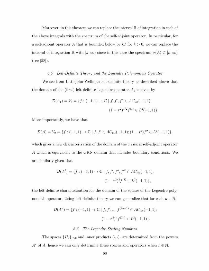
Moreover, in this theorem we can replace the interval R of integration in each of

the above integrals with the spectrum of the self-adjoint operator. In particular, for

a self-adjoint operator A that is bounded below by kI for k > 0, we can replace the

interval of integration R with [k,∞) since in this case the spectrum σ(A) ⊂ [k,∞)

(see [58]).

6.5 Left-Definite Theory and the Legendre Polynomials Operator

We see from Littlejohn-Wellman left-definite theory as described above that

the domain of the (first) left-definite Legendre operator A1 is given by

D(A1) = V3 = {f : (−1, 1)→ C | f, f ′, f ′′ ∈ ACloc(−1, 1);

(1− x2)3/2f (3) ∈ L2(−1, 1)}.

More importantly, we have that

D(A) = V2 = {f : (−1, 1)→ C | f, f ′ ∈ ACloc(−1, 1); (1− x2)f ′′ ∈ L2(−1, 1)},

which gives a new characterization of the domain of the classical self-adjoint operator

A which is equivalent to the GKN domain that includes boundary conditions. We

are similarly given that

D(A2) = {f : (−1, 1)→ C | f, f ′, f ′′, f ′′′ ∈ ACloc(−1, 1);

(1− x2)2f (4) ∈ L2(−1, 1)},

the left-definite characterization for the domain of the square of the Legendre poly-

nomials operator. Using left-definite theory we can generalize that for each n ∈ N,

D(An) = {f : (−1, 1)→ C | f, f ′, ..., f (2n−1) ∈ ACloc(−1, 1);

(1− x2)nf (2n) ∈ L2(−1, 1)}.

6.6 The Legendre-Stirling Numbers

The spaces {Hr}r>0 and inner products (·, ·)r are determined from the powers

Ar of A, hence we can only determine these spaces and operators when r ∈ N.

68

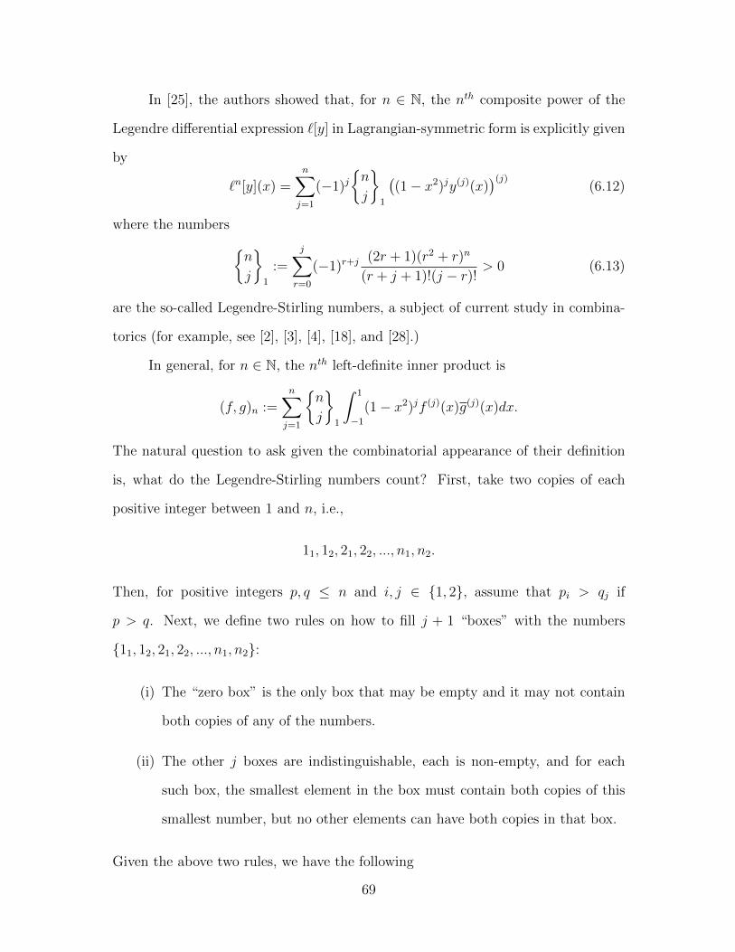
In [25], the authors showed that, for n ∈ N, the nth composite power of the

Legendre differential expression `[y] in Lagrangian-symmetric form is explicitly given

by

`n[y](x) =n∑j=1

(−1)j{n

j

}1

((1− x2)jy(j)(x)

)(j)(6.12)

where the numbers {n

j

}1

:=

j∑r=0

(−1)r+j(2r + 1)(r2 + r)n

(r + j + 1)!(j − r)!> 0 (6.13)

are the so-called Legendre-Stirling numbers, a subject of current study in combina-

torics (for example, see [2], [3], [4], [18], and [28].)

In general, for n ∈ N, the nth left-definite inner product is

(f, g)n :=n∑j=1

{n

j

}1

∫ 1

−1(1− x2)jf (j)(x)g(j)(x)dx.

The natural question to ask given the combinatorial appearance of their definition

is, what do the Legendre-Stirling numbers count? First, take two copies of each

positive integer between 1 and n, i.e.,

11, 12, 21, 22, ..., n1, n2.

Then, for positive integers p, q ≤ n and i, j ∈ {1, 2}, assume that pi > qj if

p > q. Next, we define two rules on how to fill j + 1 “boxes” with the numbers

{11, 12, 21, 22, ..., n1, n2}:

(i) The “zero box” is the only box that may be empty and it may not contain

both copies of any of the numbers.

(ii) The other j boxes are indistinguishable, each is non-empty, and for each

such box, the smallest element in the box must contain both copies of this

smallest number, but no other elements can have both copies in that box.

Given the above two rules, we have the following

69

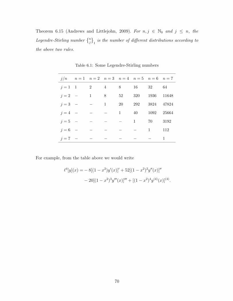
Theorem 6.15 (Andrews and Littlejohn, 2009). For n, j ∈ N0 and j ≤ n, the

Legendre-Stirling number{nj

}1

is the number of different distributions according to

the above two rules.

Table 6.1: Some Legendre-Stirling numbers

j/n n = 1 n = 2 n = 3 n = 4 n = 5 n = 6 n = 7

j = 1 1 2 4 8 16 32 64

j = 2 − 1 8 52 320 1936 11648

j = 3 − − 1 20 292 3824 47824

j = 4 − − − 1 40 1092 25664

j = 5 − − − − 1 70 3192

j = 6 − − − − − 1 112

j = 7 − − − − − − 1

For example, from the table above we would write

`4[y](x) =− 8[(1− x2)y′(x)]′ + 52[(1− x2)2y′′(x)]′′

− 20[(1− x2)3y′′′(x)]′′′ + [(1− x2)4y(4)(x)](4).

70

CHAPTER SEVEN

The Square of the Legendre Polynomials Operator

The square A2 : D(A2) ⊂ L2(−1, 1)→ L2(−1, 1) of the Legendre polynomials

operator A in L2(−1, 1) is algebraically defined by

A2f := `2[f ] (7.1)

for f ∈ D(A2), where D(A2) is defined in (1.4), and where

`2[y](x) :=((1− x2)2y′′(x)

)′′ − 2((1− x2)y′(x)

)′= (1− x2)2y(4)(x)− 8x(1− x2)y′′′(x) + (14x2 − 6)y′′(x) + 4xy′(x).

(7.2)

By standard results from functional analysis (specifically, the Hilbert space spectral

theorem), it can be shown that A2 is a self-adjoint operator in L2(−1, 1), the spec-

trum of A2 is given by σ(A2) = {n2(n+1)2 | n ∈ N0}, and the Legendre polynomials

{Pn}∞n=0 are eigenfunctions of A2.

It is natural to ask whether we can explicitly describe the functions in the

domain D(A2) similarly to how we characterize elements in D(A) as in (5.7) (or by

Theorem 5.6). In the next section, we identify A2 with a self-adjoint operator S

obtained through an application of the GKN theory.

7.1 A GKN Self-Adjoint Operator Generated by the Square of the LegendreDifferential Expression

The maximal domain ∆2,max in L2(−1, 1) associated with the square of the

Legendre expression `2[·], defined in (7.2), is given by

∆2,max := {f : (−1, 1)→ C | f, f ′, f ′′, f ′′′ ∈ ACloc(−1, 1);

f, `2[f ] ∈ L2(−1, 1)}.(7.3)

71

The sesquilinear form [·, ·]2(·) : ∆2,max × ∆2,max × (−1, 1), associated with `2[·], is

defined by

[f, g]2(x) : =((1− x2)2f ′′(x)

)′g(x)−

((1− x2)g′′(x)

)′f(x)

− (1− x2)2f ′′(x)g′(x) + (1− x2)2f ′(x)g′′(x)

− 2(1− x2)f ′(x)g(x) + 2(1− x2)f(x)g′(x) (x ∈ (−1, 1)).

(7.4)

For f, g ∈ ∆2,max and [α, β] ⊂ (−1, 1), Green’s formula for `2[·] is given by∫ β

α

`2[f ](x)g(x)dx−∫ β

α

f(x)`2[g](x) = [f, g]2(x)∣∣βα. (7.5)

By definition of ∆2,max and Holder’s inequality, we see that the limits

[f, g]2(±1) := limx→±1

[f, g]2(x)

exist and are finite for all f, g ∈ ∆2,max. Clearly

Pn ∈ ∆2,max (n ∈ N0)

where Pn is the nth degree Legendre polynomial. In particular, the functions 1 and

x belong to ∆2,max.

The endpoints x = ±1 are both regular singular points, in the sense of Frobe-

nius, of `2[·] (see Section 3.6 and [33] for explanation of the method of Frobenius.).

The Frobenius indicial equation, at either endpoint, is given by

r2(r − 1)2 = 0.

It follows, from the general Weyl theory, that each endpoint is in the limit-4 case so

the deficiency index of the minimal operator T2,min, generated by `2[·], in L2(−1, 1)

is (4, 4). Consequently, each self-adjoint operator, generated by `2[·], in L2(−1, 1) is

determined by restricting ∆2,max to four boundary conditions of the form

[f, fj]2(1)− [f, fj]2(−1) = 0, (7.6)

72

where [·, ·]2 is given in (7.4) and where {f1, f2, f3, f4} ⊂ ∆2,max is linearly independent

modulo the minimal domain ∆2,min defined by

∆2,min := {f ∈ ∆2,max | [f, g]2∣∣1−1 = 0 for all g ∈ ∆2,max},

We now identify a particular self-adjoint operator restriction S of Tmax, generated by

`2[·], having the Legendre polynomials {Pn}∞n=0 as a complete set of eigenfunctions.

For j = 1, 2, 3, 4, define fj ∈ ∆2max ∩ C4[−1, 1] by

f1(x) =

{0 near x = −1

1 near x = 1, f2(x) =

{1 near x = −1

0 near x = 1,

f3(x) =

{0 near x = −1

x near x = 1, f4(x) =

{x near x = −1

0 near x = 1.

(7.7)

Proposition 7.1. The functions {f1, f2, f3, f4} defined in (7.7) are linearly indepen-

dent modulo ∆2,min.

Proof. Calculations show that the functions log(1±x) and (1±x) log(1±x) belong

to ∆2,max, so by defining the functions gj ∈ ∆2,max ∩ C4(−1, 1) for j = 1, 2, 3, 4 as

g1(x) =

{0 near x = −1

log(1− x) near x = 1, g3(x) =

{0 near x = −1

(1− x) log(1− x) near x = 1,

g2(x) =

{log(1 + x) near x = −1

0 near x = 1, g4(x) =

{(1 + x) log(1 + x) near x = −1

0 near x = 1,

we see that

73

Table 7.1: Calculation of some sesquilinear forms

[f1, gj]2(±1) [f2, gj]2(±1) [f3, gj]2(±1) [f4, gj]2(±1)

[f1, g1]2(1) = 0 [f2, g1]2(1) = 0 [f3, g1]2(1) = −4 [f4, g1]2(1) = 0

[f1, g2]2(1) = 0 [f2, g2]2(1) = 0 [f3, g2]2(1) = 0 [f4, g2]2(1) = 0

[f1, g3]2(1) = 4 [f2,g3]2(1) = 0 [f3, g3]2(1) = 4 [f4, g3]2(1) = 0

[f1, g4]2(1) = 0 [f2, g4]2(1) = 0 [f3, g4]2(1) = 0 [f4, g4]2(1) = 0

[f1, g1]2(−1) = 0 [f2, g1]2(−1) = 0 [f3, g1]2(−1) = 0 [f4, g1]2(−1) = 0

[f1, g2]2(−1) = 0 [f2, g2]2(−1) = 0 [f3, g2]2(−1) = 0 [f4, g2]2(−1) = −4

[f1, g3]2(−1) = 0 [f2,g3]2(−1) = 0 [f3, g3]2(−1) = 0 [f4, g3]2(−1) = 0

[f1, g4]2(−1) = 0 [f2, g4]2(−1) = −4 [f3, g4]2(−1) = 0 [f4, g4]2(−1) = 4

Suppose that4∑j=1

αjfj ∈ ∆2,min;

then, by definition of ∆2,min, we see that[4∑j=1

αjfj, g

]2

∣∣∣∣∣1

−1

= 0 (g ∈ ∆2,max),

where [·, ·]2 is the sesquilinear form defined in (7.4). A calculation shows that

0 =

[4∑j=1

αjfj, g1

]2

∣∣∣∣∣1

−1

= −4α3,

so α3 = 0. Similarly, we find that

0 =

[4∑j=1

αjfj, g2

]2

∣∣∣∣∣1

−1

= 4α4,

so α4 = 0;

0 =

[4∑j=1

αjfj, g3

]2

∣∣∣∣∣1

−1

= 4α1 + 4α3 = 4α1,

so α1 = 0; and

0 =

[4∑j=1

αjfj, g4

]2

∣∣∣∣∣1

−1

= 4α2 − 4α4 = 4α2,

74

so α2 = 0. Consequently, we see that {f1, f2, f3, f4} is linearly independent modulo

∆2,min, completing the proof.

We note that the four functions {g1, g2, g3, g4} defined above are determined

by a basis of solutions of `2[y] = 0 at both x = ±1 found by the standard method of

Frobenius (see Section 3.6). Brown, Littlejohn and McCormack developed a program

in Mathematica called Frobenius which computes the coefficients of the Frobenius

solutions for arbitrary ordinary differential equations at a regular singular endpoint.

Using this program, a basis of solutions at the regular singular endpoint x = 1, valid

for −1 < x < 1, is {y1, y2, y3, y4}, is given by

y1(x) = (x− 1)− 1

4(x− 1)2 +

1

12(x− 1)3 − 1

32(x− 1)4 +

1

80(x− 1)5 − 1

192(x− 1)6

+1

448(x− 1)7 − 1

1024(x− 1)8 + · · · ,

y2(x) = 3(x− 1)− (x− 1)2 +13

36(x− 1)3 − 9

64(x− 1)4 +

23

400(x− 1)5 − 7

288(x− 1)6

+33

3136(x− 1)7 − 19

4096(x− 1)8 + · · ·

+ log |x− 1|(

(x− 1)− 1

4(x− 1)2 +

1

12(x− 1)3 − 1

32(x− 1)4 +

1

80(x− 1)5

− 1

192(x− 1)6 +

1

448(x− 1)7 − 1

1024(x− 1)8 + · · ·

),

y3(x) =1

2+

1

2(x− 1)− 1

8(x− 1)2 +

1

24(x− 1)3 − 1

64(x− 1)4 +

1

160(x− 1)5

− 1

384(x− 1)6 +

1

896(x− 1)7 + · · · , and

y4(x) = 3− 3(x− 1) +3

8(x− 1)2 − 1

12(x− 1)3 +

3

128(x− 1)4 − 3

400(x− 1)5

+1

384(x− 1)6 − 3

3136(x− 1)7 + · · ·

+ 3 log |x− 1|(

1

2+

1

2(x− 1)− 1

8(x− 1)2 +

1

24(x− 1)3 − 1

64(x− 1)4

+1

160(x− 1)5 − 1

384(x− 1)6 +

1

896(x− 1)7 − · · ·

).

75

Similarly, a basis of solutions at the endpoint x = −1, valid for −1 < x < 1 is

{z1, z2, z3, z4}, is given by

z1(x) = (x+ 1) +1

4(x+ 1)2 +

1

12(x+ 1)3 +

1

32(x+ 1)4 +

1

80(x+ 1)5 +

1

192(x+ 1)6

+1

448(x+ 1)7 +

1

1024(x+ 1)8 + · · · ,

z2(x) = 3(x+ 1) + (x+ 1)2 +13

36(x+ 1)3 +

9

64(x+ 1)4 +

23

400(x+ 1)5 +

7

288(x+ 1)6

+33

3136(x+ 1)7 +

19

4096(x+ 1)8 + · · ·

+ log |x+ 1|(

(x+ 1) +1

4(x+ 1)2 +

1

12(x+ 1)3 +

1

32(x+ 1)4 +

1

80(x+ 1)5

+1

192(x+ 1)6 +

1

448(x+ 1)7 +

1

1024(x+ 1)8 + · · ·

),

z3(x) =1

2− 1

2(x+ 1)− 1

8(x+ 1)2 − 1

24(x+ 1)3 − 1

64(x+ 1)4 − 1

160(x+ 1)5

− 1

384(x+ 1)6 − 1

896(x+ 1)7 − · · · , and

z4(x) = 3 + 3(x+ 1) +3

8(x+ 1)2 +

1

12(x+ 1)3 +

3

128(x+ 1)4 +

3

400(x+ 1)5

+1

384(x+ 1)6 +

3

3136(x+ 1)7 + · · ·

+ 3 log |x+ 1|(

1

2− 1

2(x+ 1)− 1

8(x+ 1)2 − 1

24(x+ 1)3 − 1

64(x+ 1)4

− 1

160(x+ 1)5 − 1

384(x+ 1)6 − 1

896(x+ 1)7 − · · ·

).

Recalling from Green’s formula that

[f, g]2(±1) := limx→±1

[f, g]2(x),

it is clear that the boundary conditions

[f, f1]2(1) = [f, f3]2(1) = [f, f2]2(−1) = [f, f4]2(−1) = 0

are equivalent to the boundary conditions

[f, 1]2(±1) = [f, x]2(±1) = 0.

We are now in a position to the define the operator S which we show later (see

Section 7.4) to be equal to the operator A2, given in (7.1) and (1.4). Indeed, let

76

S : D(S) ⊂ L2(−1, 1)→ L2(−1, 1) be defined by

Sf = `2[f ] := `[`[f ]]

f ∈ D(S),

(7.8)

where the domain D(S) of S is defined in (1.5) or more succinctly as

D(S) := {f ∈ ∆2,max | [f, 1]2(±1) = [f, x]2(±1) = 0}.

By the GKN theorem, S is self-adjoint in L2(−1, 1). Moreover, notice that for

f ∈ ∆2,max,

[f, 1]2(x) =((1− x2)2f ′′(x)

)′ − 2(1− x2)f ′(x) (7.9)

and

[f, x]2(x) =((1− x2)2f ′′(x)

)′x− (1− x2)2f ′′(x)

− 2x(1− x2)f ′(x) + 2(1− x2)f(x)

= x[f, 1]2(x)− (1− x2)2f ′′(x) + 2(1− x2)f(x).

(7.10)

From (7.9) and (7.10), it is easy to see that the Legendre polynomials {Pn}∞n=0 satisfy

[Pn, 1]2(±1) = [Pn, x]2(±1) = 0,

that is to say, the Legendre polynomials {Pn}∞n=0 ⊂ D(S). Moreover,

`2[Pn] = `[`[Pn]] = n(n+ 1)`[Pn] = n2(n+ 1)2Pn (n ∈ N0).

From [52] and standard results in spectral theory, the following result holds.

Theorem 7.2. The operator S, defined in (7.8) and (1.5), is an unbounded self-

adjoint operator in L2(−1, 1). The Legendre polynomials {Pn}∞n=0 form a complete

set of (orthogonal) eigenfunctions of S in L2(−1, 1). The spectrum σ(S) of S is

discrete and given explicitly by

σ(S) = {n2(n+ 1)2 | n ∈ N0}.

77

7.2 Statements of the Main Theorems

We prove four main theorems in this chapter.

Theorem 7.3. Let D(A2) and D(S) be given, respectively, as in (1.4) and (1.5). Then

D(A2) = D(S).

Proof. See Section 7.4.

Theorem 7.4. Let B and D(S) be given, respectively, as in (1.2) and (1.5). Then

B = D(S).

Proof. See Section 7.5.

Theorem 7.5. Let D(S) and D be given, respectively, as in (1.5) and (1.6). Then

D = D(S).

Proof. See Section 7.6.

From these three theorems, we obtain our main result, namely

Theorem 7.6. Let ∆2,max, given in (7.3), be the maximal domain of the formal square

`2[·] of the Legendre differential expression defined by

`2[y](x) =((1− x2)2y′′(x)

)′′ − 2((1− x2)y′(x)

)′(x ∈ (−1, 1)) (7.11)

and let [·, ·]2 be the associated sesquilinear form for `2[·] given in (7.4). Define the

operator T : D(T ) ⊂ L2(−1, 1)→ L2(−1, 1) by

(Tf)(x) = `2[f ](x) (a.e. x ∈ (−1, 1))

f ∈ D(T ) := D(A2),

where D(A2), algebraically defined in (1.4), is the domain of the square of the Leg-

endre polynomials operator A defined in (5.7). That is to say, T is the square of

the classical Legendre polynomials operator A, given in (5.6) and (5.7). Then the

following statements are equivalent:

78

(i) f ∈ D(T );

(ii) f, f ′, f ′′, f ′′′ ∈ ACloc(−1, 1) and (1− x2)2f (4) ∈ L2(−1, 1);

(iii) f ∈ ∆2,max and [f, 1]2(±1) = [f, x]2(±1) = 0;

(iv) f ∈ ∆2,max and limx→±1

(1− x2)f ′(x) = limx→±1

((1− x2)2f ′′(x)

)′= 0.

Moreover, T is a self-adjoint operator in L2(−1, 1) having the Legendre polynomi-

als {Pn}∞n=0 as a complete set of eigenfunctions in L2(−1, 1) and having discrete

spectrum σ(T ) explicitly given by

σ(T ) = {n2(n+ 1)2 | n ∈ N0}.

7.3 A Key Integral Inequality

A key result in our analysis below is the following operator inequality estab-

lished by Chisholm and Everitt in [12]. Both the theorem and its corollary are

referred to as the “CE Theorem.”

Theorem 7.7. Let (a, b) be an open interval of the real line (bounded or unbounded)

and let w be a positive Lebesgue measurable function that is positive a.e. x ∈ (a, b).

Suppose ϕ, ψ : (a, b)→ C satisfy the conditions

(i) ϕ, ψ ∈ L2loc((a, b);w);

(ii) there exists c ∈ (a, b) such that ϕ ∈ L2((a, c];w) and ψ ∈ L2([c, b);w);

(iii) for all [α, β] ⊂ (a, b),∫ β

α

|ϕ(x)|2w(x)dx > 0 and

∫ β

α

|ψ(x)|2w(x)dx > 0.

Define the linear operators A,B : L2((a, b);w)→ L2loc((a, b);w) by

(Af)(x) = ϕ(x)

∫ b

x

ψ(t)f(t)w(t)dt (t ∈ (a, b); f ∈ L2((a, b);w)),

79

and

(Bf)(x) = ψ(x)

∫ x

a

ϕ(t)f(t)w(t)dt (t ∈ (a, b); f ∈ L2((a, b);w)).

Let K : (a, b)→ (0,∞) be given by

K(x) =

(∫ x

a

|ϕ(t)|2w(t)dt

) 12(∫ b

x

|ψ(t)|2w(t)dt

) 12

(t ∈ (a, b)),

and define K ∈ [0,∞] by

K := supx∈(a,b)

K(x). (7.12)

Then a necessary and sufficient condition that A and B are both bounded operators

from L2((a, b);w) into L2((a, b);w) is that

0 < K <∞.

Moreover, the following inequalities hold

||Af || ≤ 2K||f || (f ∈ L2((a, b);w)) (7.13)

||Bg|| ≤ 2K||g|| (g ∈ L2((a, b);w)) (7.14)

where the number K is defined by (7.12). In general, the number 2K appearing in

both (7.13) and (7.14) is best possible for these inequalities to hold.

Corollary 7.8. Suppose the functions ϕ and ψ are as in the above theorem. Let

g ∈ L2((a, b);w). Define

g1(x) = ϕ(x)

∫ b

x

ψ(x)g(x)w(x)dx (x ∈ (a, b)),

g2(x) = ψ(x)

∫ x

z

ϕ(x)g(x)w(x)dx (x ∈ (a, b)).

If K <∞, where K is defined as in the previous theorem, then gr ∈ L2((a, b);w) for

r = 1, 2.

We note that Theorem 7.7, proven by Chisholm and Everitt in 1970, was

extended in 1999 by Chisholm, Everitt, and Littlejohn to the spaces Lp((a, b);w)

80

and Lq((a, b);w) where p, q > 1 are conjugate indices; see [12]. Both Theorem 7.7

and its generalization in [12] have seen several applications including a new proof of

the classical Hardy integral inequality [31] and numerous applications to orthogonal

polynomials. Several more applications of the CE Theorem will be given in this

paper. Indeed, the Theorem 7.7 proves to be an indispensable tool in our analysis

below.

7.4 Proof of Theorem 7.3

We now prove Theorem 7.3, namely, that D(A2) = D(S), where D(A2) is

defined in (1.4) and D(S) is given in (1.5). Throughout this section, we assume that

f is a real-valued function on (−1, 1).

Proof. We first show that D(S) ⊂ D(A2). Let f ∈ D(S). We know that

(i) f, f ′, f ′′, f ′′′ ∈ ACloc(−1, 1);

(ii) f ∈ L2(−1, 1);

(iii) `2[f ] ∈ L2(−1, 1), where `2[·] is defined by (7.2);

(iv) [f, 1]2(±1) = 0, where [·, 1]2(·) is given in (7.9);

(v) [f, x]2(±1) = 0, where [·, x]2(·) is given in (7.10).

Taking into account the definition of D(A) in (5.7) and D(A2) in (1.4), we need to

show that

(a) f, f ′ ∈ ACloc(−1, 1);

(b) f ∈ L2(−1, 1);

(c) `[f ] = − ((1− x2)f ′)′ = −(1 − x2)f ′′ + 2xf ′ ∈ L2(−1, 1); in fact, we will

show that `[f ] ∈ AC[−1, 1];

81

(d) limx→±1

(1− x2)f ′(x) = 0;

(e) `[f ], `′[f ] ∈ ACloc(−1, 1);

(f) `2[f ] ∈ L2(−1, 1);

(g) limx→±1

(1− x2)`′[f ] := limx→±1

(1− x2)((1− x2)f ′′′(x)− 4xf ′′(x)− 2f ′(x)

)= 0.

Clearly, (a), (b), and (f) are satisfied by (i), (ii), and (iii). As for (g), note that

−(1− x2)`′[f ](x) = (1− x2)((1− x2)f ′′′(x)− 4xf ′′(x)− 2f ′(x)

)= (1− x2)2f ′′′(x)− 4x(1− x2)f ′′(x)− 2(1− x2)f ′(x)

=((1− x2)2f ′′(x)

)′ − 2(1− x2)f ′(x)

= [f, 1]2(x),

(7.15)

so (g) follows from (iv) above. Moreover, by (i) and the fact that the product of

a polynomial and a function g ∈ ACloc(−1, 1) also belongs to ACloc(−1, 1), we see

that (e) follows, as

`[f ](x) = −(1− x2)f ′′(x) + 2xf ′(x)

and

`′[f ](x) = −(1− x2)f ′′′(x) + 4xf ′′(x) + 2f ′(x).

To show (c) note that, by (iii),

`2[f ](x) = `[`[f ]](x) = −((1− x2)`′[f ](x)

)′ ∈ L2(−1, 1). (7.16)

We now apply the CE Theorem on the interval [0, 1) with ψ(x) = 1, ϕ(x) = 11−x2 ,

and w(x) = 1; note that ϕ ∈ L2(0, 1

2

]and ψ ∈ L2

[12, 1). A calculation shows that

K2(x) =

∫ x

0

dt

(1− t2)2·∫ 1

x

dt (x ∈ (0, 1))

=1

1− t2

∣∣∣∣x0

· (x− 1)

= − 1

1 + x,

82

hence K is finite. Therefore, we see from Theorem 7.7 that

ϕ(x)

∫ 1

x

ψ(t)`2[f ](t)w(t)dt =1

1− x2

∫ 1

x

`2[f ](t)dt

= − 1

1− x2

∫ 1

x

((1− x2)`′[f ](x)

)′dt

= − 1

1− x2(1− x2)`′[f ](x)

∣∣∣∣1x

=1

1− x2(

(1− x2)`′[f ](x)− limx→1

(1− x2)`′[f ](x))

∈ L2[0, 1),

(7.17)

By (iv) and (7.15), we know

limx→1

(1− x2)`′[f ](x) = 0.

Hence (7.17) simplifies to

`′[f ] ∈ L2[0, 1).

A similar application of the CE Theorem on (−1, 0] reveals that `′[f ] ∈ L2(−1, 0]

and thus we see that

`′[f ] ∈ L2(−1, 1).

It follows that

`[f ] ∈ AC[−1, 1] ⊂ L2(−1, 1),

establishing (c). It remains to show that (d) holds. To this end, observe from (2.6)

and (7.2) that ((1− x2)2f ′′(x)

)′′= `2[f ](x)− 2`[f ](x).

Consequently, from (c) and (f),

((1− x2)2f ′′(x)

)′′ ∈ L2(−1, 1),

from which we see that

((1− x2)2f ′′(x)

)′, (1− x2)2f ′′(x) ∈ AC[−1, 1].

83

In particular, we see that the limits

limx→±1

(1− x2)2f ′′(x) (7.18)

and

limx→±1

((1− x2)2f ′′(x)

)′(7.19)

exist and are finite. Moreover, from (iv), (v), and (7.10), we see that

0 = limx→±1

(x[f, 1]2(x)− [f, x]2(x)) = limx→±1

((1− x2)2f ′′(x)− 2(1− x2)f(x)

). (7.20)

Thus, from (7.18), we can say that

limx→±1

(1− x2)f(x) := r

exists and is finite. We claim that r = 0; to show this, we deal with the limit as

x→ 1; a similar proof can be made as x→ −1. Suppose to the contrary that r 6= 0;

without loss of generality, suppose r > 0. Then there exists x∗ > 0 such that

(1− x2)f(x) ≥ r

2for x ∈ [x∗, 1).

In this case, however,

∞ >

∫ 1

−1|f(x)|2dx ≥

∫ 1

x∗|f(x)|2dx ≥

(r2

)2 ∫ 1

x∗

dx

(1− x2)2=∞,

contradicting (ii). Hence it follows that

limx→±1

(1− x2)f(x) = 0.

Consequently, we see from (7.19), that

limx→±1

(1− x2)2f ′′(x) = 0 (7.21)

and hence

limx→±1

(1− x)2f ′′(x) = 0. (7.22)

84

We are now in position to prove part (d). We show that

limx→1

(1− x2)f ′(x) = 0; (7.23)

a similar argument establishes the limit as x → −1. Let ε > 0. From (7.22), there

exists x∗ ∈ (0, 1) such that

|(1− x)2f ′′(x)| < ε

2for x ∈ [x∗, 1).

Integrating this inequality over [x∗, x] ⊂ [x∗, 1) yields

ε

2(1− x∗)+f ′(x∗)− ε

2(1− x)< f ′(x) <

ε

2(1− x)+f ′(x∗)− ε

2(1− x∗)for x ∈ [x∗, 1).

Multiplying this inequality by (1− x2) yields

(1− x2)(f ′(x∗) +

ε

2(1− x∗)

)− ε(1 + x)

2

< (1− x2)f ′(x) <ε(1 + x)

2+ (1− x2)

(f ′(x∗)− ε

2(1− x∗)

).

Letting x→ 1, we obtain

−ε ≤ limx→1

(1− x2)f ′(x) ≤ ε,

and this establishes (7.23). This completes the proof that D(S) ⊂ D(A2).

We now show that D(A2) ⊂ D(S). Let f ∈ D(A2). Then f ∈ D(A) so

f, f ′ ∈ ACloc(−1, 1) (7.24)

and

f ∈ L2(−1, 1). (7.25)

Moreover, since `[f ] ∈ D(A), it follows that

`2[f ] = `[`[f ]] ∈ L2(−1, 1), (7.26)

`[f ] = −(1− x2)f ′′ + 2xf ′ ∈ ACloc(−1, 1), (7.27)

and

`′[f ] = −(1− x2)f ′′′ + 4xf ′ + 2f ′ ∈ ACloc(−1, 1). (7.28)

It is well known that if f, g ∈ ACloc(1,−1), then

85

(a)′ f + g ∈ ACloc(−1, 1);

(b)′ fg ∈ ACloc(−1, 1);

(c)′ If g > 0 on (−1, 1), then fg∈ ACloc(−1, 1).

In particular, from (7.24) and (b)′ we see that 2xf ′ ∈ ACloc(−1, 1). Combining this

with (a)′ and (7.27), we obtain (1 − x2)f ′′ ∈ ACloc(−1, 1). Since 1 − x2 > 0 on

(−1, 1) we infer from (c)′ that

f ′′ ∈ ACloc(−1, 1). (7.29)

Continuing, −4xf ′′ − 2f ′ ∈ ACloc(−1, 1) so from (a)′ and (7.28), we have that

(1− x2)f ′′′ ∈ ACloc(−1, 1) and it follows that

f ′′′ ∈ ACloc(−1, 1). (7.30)

By definition of D(A) and the fact that `[f ] ∈ D(A), we see that

limx→±1

(1− x2)`′[f ](x) = 0;

consequently, in view of (7.15), we see that

0 = limx→±1

[f, 1]2(x) = limx→±1

(((1− x2)2f ′′(x)

)′ − 2(1− x2)f ′(x)). (7.31)

Furthermore, since f ∈ D(A), we have

limx→±1

(1− x2)f ′(x) = 0, (7.32)

so from (7.31), we see that

limx→±1

((1− x2)2f ′′(x)

)′′= 0.

To finish the proof, we need to show that

0 = [f, x]2(±1)

= limx→±1

(((1− x2)2f ′′(x)

)′x− (1− x2)2f ′′(x)− 2x(1− x2)f ′(x) + 2(1− x2)f(x)

)= lim

x→±1

(−(1− x2)2f ′′(x) + 2(1− x2)f(x)

)by (7.31).

(7.33)

86

We note again, from Green’s formula (7.5), that the limits in (7.33) exist and are

finite. Since f ∈ D(A), we see from Theorem 5.6, part (v) that f ∈ AC[−1, 1] and

hence

limx→±1

(1− x2)f(x) = 0. (7.34)

Thus, proving (7.33) reduces to showing

limx→±1

(1− x2)2f ′′(x) = 0.

We show that

limx→1

(1− x2)2f ′′(x) = 0; (7.35)

a similar argument will show

limx→−1

(1− x2)2f ′′(x) = 0.

Suppose to the contrary that

limx→1

(1− x2)2f ′′(x) = c 6= 0;

without loss of any generality, we can suppose that c > 0. Then there exists

x∗ ∈ (0, 1) such that

(1− x2)2f ′′(x) ≥ r :=c

2on [x∗, 1);

that is,

f ′′(x) ≥ R

(1− x)2on [x∗, 1)

for some R > 0. Integrating this inequality over [x, x∗] ⊂ [x∗, 1) yields

f ′(x) ≥ R

∫ x

x∗

dt

(1− t)2+ f ′(x∗) =

R

1− x+ f ′(x∗)− R

1− x∗.

Consequently,

(1− x2)f ′(x) ≥ R(1 + x) +

(f ′(x∗)− R

1− x∗

)(1− x2)→ 2R > 0 (as x→ 1),

87

contradicting (7.32). It follows that (7.35) holds and this proves (7.33). A similar

proof establishes [f, x]2(−1) = 0 which proves (7.33). Combining (7.24), (7.25),

(7.26), (7.29), (7.30), (7.31) and (7.33), we see that f ∈ D(A2) implies f ∈ D(S).

This completes the proof of the theorem.

7.5 Proof of Theorem 7.4

In order to prove Theorem 7.4, we first need to establish three preliminary

facts, the first of which is the following result.

Lemma 7.9. If f ∈ D(S), then

1

1− x2((1− x2)2f ′′(x)

)′ ∈ L2(−1, 1). (7.36)

Proof. Let f ∈ D(S) = D(A2) so f ′ ∈ L2(−1, 1), [f, 1]2(±1) = 0, and `2[f ] ∈ L2(−1, 1).

We apply the CE Theorem on [0, 1) with ψ(x) = 1, ϕ(x) = − 11−x2 , and w(x) = 1.

These functions satisfy the conditions of this theorem on [0, 1) so

− 1

1− x2

∫ 1

x

`2[f ](t)dt ∈ L2(0, 1).

However, using (7.9) and (7.11), a calculation shows

− 1

1− x2

∫ 1

x

`2[f ](t)dt = − 1

1− x2

∫ 1

x

[((1− t2)2f ′′(t)

)′′ − 2((1− t2)f ′(t)

)′]dt

= − 1

1− x2[limx→1

(((1− x2)2f ′′(x)

)′ − 2(1− x2)f ′(x))]

+1

1− x2[(

(1− x2)2f ′′(x))′ − 2(1− x2)f ′(x))

]= − 1

1− x2[limx→1

[f, 1]2(x)−((1− x2)2f ′′(x)

)′+ 2(1− x2)f ′(x)

]=

1

1− x2((1− x2)2f ′′(x)

)′ − 2f ′(x).

A similar calculation shows that

1

1− x2((1− x2)2f ′′(x)

)′ − 2f ′(x) ∈ L2(−1, 0]

and hence

1

1− x2((1− x2)2f ′′(x)

)′ − 2f ′(x) ∈ L2(−1, 1).

88

Since f ′ ∈ L2(−1, 1), we see, by linearity, that

1

1− x2((1− x2)2f ′′(x)

)′ ∈ L2(−1, 1).

Lemma 7.10. For f ∈ D(S), we have

limx→±1

(1− x2)2f ′′(x) = 0. (7.37)

Proof. Let f ∈ D(S) = D(A2). Since f ∈ D(A), we have f ∈ AC[−1, 1], so

limx→±1

(1− x2)f(x) = 0. (7.38)

Furthermore, we have

0 = limx→±1

[f, 1]2(x) = limx→±1

(((1− x2)2f ′′(x)

)′ − 2(1− x2)f ′(x)). (7.39)

Consequently, from (7.10), (7.38), and (7.39), we find that

0 = limx→±1

[f, x]2(x) = limx→±1

(x[f, 1]2(x)− (1− x2)2f ′′(x) + 2(1− x2)f(x)

)= − lim

x→±1(1− x2)2f ′′(x).

The last preliminary result is the following theorem. Since D(S) = D(A2),

this next result generalizes the well-known result for D(A) established in Theorem

5.6, part (v).

Theorem 7.11. If f ∈ D(S), then

f ′′ ∈ L2(−1, 1).

Moreover,

pf ′′ ∈ L2(−1, 1) (7.40)

for any bounded, Lebesgue measurable function p, including any polynomial.

89

Proof. Once we establish f ′′ ∈ L2(−1, 1), the statement in (7.40), for any bounded

measurable function, follows clearly. Let f ∈ D(S). We prove that f ′′ ∈ L2(0, 1); a

similar proof will establish f ′′ ∈ L2(−1, 0) and prove the theorem. We again use the

CE Theorem with ψ(x) = 1− x2, ϕ(x) = 1(1−x2)2 , and w(x) = 1 on [0, 1). Indeed,

from the CE Theorem and (7.36), we find that

− 1

(1− x2)2

∫ 1

x

(1− t2)(

1

1− t2((1− t2)2f ′′(t)

)′)dt ∈ L2(0, 1).

However, from Lemma 7.9,

− 1

(1− x2)2

∫ 1

x

(1− t2)(

1

1− t2((1− t2)2f ′′(t)

)′)dt

= − 1

(1− x2)2(

limx→1

(1− x2)f ′′(x)− (1− x2)2f ′′(x))

= f ′′(x).

We are now in position to prove Theorem 7.4, specifically B = D(S), where B

is defined in (1.2) and D(S) is given in (1.5).

Proof. We first prove that B ⊂ D(S). Let f ∈ B. We assume that f is real-valued

on (−1, 1). We begin by showing, using the CE Theorem, that the condition

(1− x2)2f (4) ∈ L2(−1, 1)

implies the two conditions

(1− x2)f ′′′ ∈ L2(−1, 1) (7.41)

and

f ′′ ∈ L2(−1, 1). (7.42)

Regarding (7.41), we will show

(1− x2)f ′′′ ∈ L2(0, 1); (7.43)

90

a similar proof will yield

(1− x2)f ′′′ ∈ L2(−1, 0), (7.44)

and, together, they establish (7.41). Since (1 − x2)2f (4) ∈ L2(0, 1), we use the CE

Theorem on [0, 1) with

ϕ(x) =1

(1− x2)2, ψ(x) = 1− x2, and w(x) = 1 (x ∈ [0, 1)).

It follows that

(1− x2)f ′′′(x) = (1− x2)∫ x

0

1

(1− t2)2(1− t2)2f (4)(t)dt+ f ′′′(0)(1− x2) ∈ L2(0, 1).

To see (7.42), we apply the CE Theorem once again on [0, 1) to prove that

f ′′ ∈ L2(0, 1);

a similar argument will show that f ′′ ∈ L2(−1, 0). To this end, let

ϕ(x) =1

1− x2, ψ(x) = 1, and w(x) = 1 (x ∈ [0, 1)).

In this case, we see that

f ′′(x) =

∫ x

0

1

1− t2((1− t2)f ′′′(t)

)dt+ f ′′(0) ∈ L2(0, 1).

Consequently, we see that

f, f ′ ∈ AC[−1, 1] ⊂ L2(−1, 1).

Moreover, it is clear that g(x)(1− x2)f ′′′(x), g(x)f ′′(x), and g(x)f ′(x) all belong to

L2(−1, 1) for any bounded, measurable function g on (−1, 1). Hence

`2[f ](x) = (1−x2)2f (4)(x)−8x(1−x2)f ′′′(x)+(14x2−6)f ′′(x)+4xf ′(x) ∈ L2(−1, 1).

It remains to show that

limx→±1

[f, 1]2(x) = limx→±1

[f, x]2(x) = 0. (7.45)

91

Since 1, x ∈ ∆2,max, we see from Green’s formula in (7.5) that the limits in (7.45)

both exist and are finite. Now f ′ ∈ AC[−1, 1] so

limx→±1

(1− x2)f ′(x) = 0.

Consequently,

limx→±1

[f, 1]2(x) = limx→±1

(((1− x2)2f ′′(x)

)′ − 2(1− x2)f ′(x))

= limx→±1

((1− x2)2f ′′(x)

)′.

We claim that

limx→1

((1− x2)2f ′′(x)

)′= 0; (7.46)

a similar proof will establish

limx→−1

((1− x2)2f ′′(x)

)′= 0.

Suppose to the contrary that

limx→1

((1− x2)2f ′′(x)

)′= c 6= 0;

we can assume that c > 0. It follows that there exists x∗ ∈ (0, 1) such that

((1− x2)2f ′′(x)

)′ ≥ r :=c

2> 0 (x ∈ [x∗, 1)). (7.47)

Note that since

((1− x2)2f ′′(x)

)′= (1− x2)2f ′′′(x)− 4x(1− x2)f ′′(x), (7.48)

we see that the inequality in (7.47) can be rewritten as

(1− x2)f ′′′(x)− 4xf ′′(x) ≥ r

1− x2for x ∈ [x∗, 1). (7.49)

However, from (7.41) and (7.42), we know that

(1− x2)f ′′′ − 4xf ′′ ∈ L2(−1, 1)

92

so the inequality in (7.49) is not possible. Hence (7.46) is established and thus

limx→±1

[f, 1]2(x) = 0.

We now show that

limx→±1

[f, x]2(x) = 0. (7.50)

Since the argument for x→ −1 mirrors the proof for x→ 1, we will only show that

limx→1

[f, x]2(x) = 0.

Now, since f ∈ AC[−1, 1], we see that

limx→1

(1− x2)f(x) = 0;

moreover, using (7.46),

limx→1

[f, x]2(x) = limx→1

(x[f, 1]2(x)− (1− x2)2f ′′(x) + 2(1− x2)f(x)

)= − lim

x→1(1− x2)2f ′′(x).

Suppose that

limx→1

(1− x2)2f ′′(x) = d 6= 0;

we can assume that d > 0. Then, with a possibly different x∗ as given in the above

argument, there exists an x∗ ∈ (0, 1) with

(1− x2)2f ′′(x) ≥ d′ :=d

2(x ∈ [x∗, 1)).

Hence

f ′′(x) ≥ d′

(1− x2)2(x ∈ [x∗, 1)).

However, this implies that f ′′ 6∈ L2(0, 1), contradicting (7.42). Thus (7.50) is estab-

lished and this completes the proof that B ⊂ D(S).

We now prove that D(S) ⊂ B. Let f ∈ D(S). We need only to show that

(1− x2)2f (4) ∈ L2(−1, 1). (7.51)

93

Since by Theorem 7.10 we know that f ′′ ∈ L2(−1, 1), we see that gf ′′ ∈ L2(−1, 1)

for any bounded, measurable function g on (−1, 1). In particular, it is the case that

4xf ′′ ∈ L2(−1, 1) (7.52)

and

(14x2 − 6)f ′′ ∈ L2(−1, 1). (7.53)

By (7.36) (see also (7.48)),

(1− x2)f ′′′(x)− 4xf ′′(x) =1

1− x2((1− x2)2f ′′(x)

)′ ∈ L2(−1, 1). (7.54)

By linearity, it follows from (7.52) and (7.54) that

(1− x2)f ′′′ ∈ L2(−1, 1).

Consequently, g(1−x2)f ′′′ ∈ L2(−1, 1) for every bounded, measurable function g on

(−1, 1);in particular,

8x(1− x2)f ′′′ ∈ L2(−1, 1). (7.55)

Furthermore, since f ′ ∈ L2(−1, 1), it follows that

4xf ′(x) ∈ L2(−1, 1). (7.56)

Finally, since `2[f ] ∈ L2(−1, 1), we see from (1.3), (7.53), (7.55), and (7.56) that

(1− x2)2f (4) = `2[f ] + 8x(1− x2)f ′′′ − (14x2 − 6)f ′′ − 4xf ′ ∈ L2(−1, 1).

This establishes (7.51) and proves D(S) ⊂ B. This completes the proof of Theorem

7.4.

7.6 Proof of Theorem 7.5

We now prove Theorem 7.5, namely D(S) = D, where D(S) is given in (1.5)

and D is defined in (1.6).

94

Proof. Since functions f in both D(S) and D satisfy the “maximal domain” condi-

tions f (j) ∈ ACloc(−1, 1) (j = 0, 1, 2, 3), f ∈ L2(−1, 1), and `2[f ] ∈ L2(−1, 1), we

need only to prove that the other properties in their definitions hold.

We first show that D(S) ⊂ D2. Let f ∈ D(S) = D(A2). Then f ∈ D(A) so

limx→±1

(1− x2)f ′(x) = 0. (7.57)

Moreover,

0 = [f, 1]2(±1)

= limx→±1

(((1− x2)2f ′′(x)

)′ − 2(1− x2)f ′(x))

= limx→±1

((1− x2)2f ′′(x)

)′.

(7.58)

The identities in (7.57) and (7.58) prove that f ∈ D, hence D(S) ⊂ D.

We now prove that D ⊂ D(S). Let f ∈ D. Clearly,

[f, 1]2(±1) = limx→±1

(((1− x2)2f ′′(x)

)′ − 2(1− x2)f ′(x))

= 0, (7.59)

so we need to show that

limx→±1

[f, x]2(±1) = 0. (7.60)

We remark that the limits in (7.60) exist (by Green’s formula) and are finite.

We claim that `′[f ] ∈ L2(−1, 1). To see this, recall the two representations of

`2[·]: the one given in (1.3) and the one given in (7.15). Since `2[f ] ∈ L2(−1, 1), we

apply the CE Theorem on [0, 1) with ϕ(x) = (1− x2)−1, ψ(x) = 1, and w(x) = 1 to

obtain

1

1− x2

∫ 1

x

`2[f ](t)dt ∈ L2(0, 1).

However, from (1.3) and (7.15), we see that

1

1− x2

∫ 1

x

`2[f ](t)dt

=1

1− x2(

limx→1

(((1− x2)2f ′′(x)

)′ − 2(1− x2)f ′(x))

+ (1− x2)`′[f ](x))

= `′[f ](x) by (7.59);

95

a similar calculation shows that `′[f ] ∈ L2(−1, 0), hence `[f ] ∈ AC[−1, 1] ⊂ L2(−1, 1).

We again apply the CE Theorem on [0, 1) with ϕ(x) = (1 − x2)−1, ψ(x) = 1, and

w(x) = 1 to obtain

1

1− x2

∫ 1

x

`[f ](t)dt ∈ L2(0, 1).

Another calculation shows that

1

1− x2

∫ 1

x

`[f ](t)dt = − 1

1− x2

∫ 1

x

((1− t2)f ′(t)

)′dt

= − 1

1− x2(

limx→1

(1− x2)f ′(x)− (1− x2)f ′(x))

= f ′(x) by definition of D;

a similar argument shows that f ′ ∈ L2(−1, 0). Hence

f ′ ∈ L2(−1, 1). (7.61)

Thus, f ∈ AC[−1, 1] and

limx→±1

(1− x2)f(x) = 0. (7.62)

From (7.59) and (7.62), we see that

limx→±1

[f, x]2(x) = limx→±1

(x[f, 1](x)− (1− x2)2f ′′(x) + 2(1− x2)f(x)

)= − lim

x→±1(1− x2)2f ′′(x).

To establish (7.60), it now suffices to prove that

limx→±1

(1− x2)2f ′′(x) = 0. (7.63)

Since the proof as x→ −1 is similar to the proof that x→ 1, we will only show that

limx→1

(1− x2)2f ′′(x) = 0.

By way of contradiction, suppose that

limx→1

(1− x2)2f ′′(x) = c 6= 0;

96

without loss of generality, we may assume that c > 0. Then there exists x∗ ∈ (0, 1)

such that

f ′′(x) ≥ c

2(1− x2)2≥ c

8(1− x)2for x ∈ [x∗, 1).

Integrating this inequality over [x∗, x] ⊂ [x∗, 1) yields

f ′(x) ≥ c

8(1− x)+ f ′(x∗)− c

8(1− x∗)(x ∈ [x∗, 1)).

However, this contradicts (7.61). It follows that (7.63) holds and this, in turn,

establishes (7.60). Consequently, D ⊂ D(S) and this completes the proof of the

theorem.

As revealed in the proofs of Theorems 7.3, 7.4, 7.5, and 7.10, we have the

following interesting result.

Corollary 7.12. If f ∈ D(A2) = D(S) = B = D, then

(i) f ′′ ∈ L2(−1, 1) so f, f ′ ∈ AC[−1, 1];

(ii) `′[f ] ∈ L2(−1, 1) and `[f ] ∈ AC[−1, 1].

We end this section with an important remark. As discussed in Section 7.1, the

minimal operator T2,min in L2(−1, 1) generated by `2[·] has deficiency index (4, 4).

From the GKN Theorem (see [52]), GKN boundary conditions for any self-adjoint

extension of T2,min in L2(−1, 1) are restrictions of the maximal domain ∆2,max and

have the appearance (see (7.6))

[f, fj]2(1)− [f, fj]2(−1) = 0 (f ∈ ∆2,max, j = 1, 2, 3, 4),

where {fj}4j=1 ⊂ ∆2,max are linearly independent modulo the minimal domain ∆2,min.

Taking into account [·, ·]2, defined in (7.4), it is clear that the boundary conditions

given in (1.6) are not GKN boundary conditions. [48]

97

CHAPTER EIGHT

The nth Power of the Legendre Polynomials Operator

Recall `n[·], the nth composite power of the Legendre differential expression

`[·] for n ∈ N given in (6.12). The expression in (6.12) is the key in generating the

domain D(An) of An given in (1.1).

We give the following

Conjecture 8.1. Let A denote the Legendre polynomials self-adjoint operator defined

in (5.6) and (5.7). For n ∈ N, let `n[·] be given as in (6.12) and let [·, ·]n be the

sesquilinear form associated with the maximal domain ∆n,max of `n[·] in L2(−1, 1).

Then An = Bn = Cn = Dn, where

(i) An := D(An),

(ii) Bn := {f : (−1, 1)→ C | f, f ′, ..., f (2n−1) ∈ ACloc(−1, 1);

(1− x2)nf (2n) ∈ L2(−1, 1)},

(iii) Cn := {f : (−1, 1)→ C | f, f ′, ..., f (2n−1) ∈ ACloc(−1, 1); f, `n[f ] ∈ L2(−1, 1);

[f, xj]n(±1) = 0 for j = 0, 1, 2, ..., n− 1}, and

(iv) Dn := {f : (−1, 1)→ C | f, f ′, ..., f (2n−1) ∈ ACloc(−1, 1); f, `n[f ] ∈ L2(−1, 1);

limx→±1

((1− x2)jy(j)(x)

)(j−1)= 0 for j = 1, 2, ..., n}.

By repeated applications of the CE Theorem, it is not difficult to establish

that if f ∈ Bn, then f (n) ∈ L2(−1, 1); this result, proven below in the proof of

Theorem 8.2, generalizes Theorem 5.6, part (iii) (n = 1) and Corollary 7.11, part (i)

(n = 2).

We remark that, in (iii) above, we can replace the monomials {xj}n−1j=0 by

the Legendre polynomials {Pj}n−1j=0 . One of the difficulties in our efforts to try and

98

prove this conjecture lies in the fact that the corresponding sesquilinear form [·, ·]n,

associated with the nth power `n[·], is unwieldy at the present time.

Theorem 8.2. Let Bn and Dn be defined as in Conjecture 8.1 above. Then Bn ⊆ Dn.

Proof. To show that Bn ⊆ Dn, let f ∈ Bn. Then (1 − x2)nf (2n) ∈ L2(−1, 1). We

first show by using the CE Theorem that this implies (1−x2)n−1f (2n−1) ∈ L2(−1, 1).

Lemma 8.3. (1− x2)nf (2n) ∈ L2(−1, 1) =⇒ (1− x2)n−1f (2n−1) ∈ L2(−1, 1).

Proof. Since f is absolutely continuous, so are all its derivatives, hence∫ x

0

1

(1− t2)n(1− t2)nf (2n)(t)dt = f (2n−1)(x)− f (2n−1)(0),

by letting

ϕ(t) =1

(1− t2)n

and noting that

(1− t2)nf (2n) ∈ L2(−1, 1),

so

f (2n−1)(x) = f (2n−1)(0) +

∫ x

0

1

(1− t2)n(1− t2)nf (2n)(t)dt.

Multiply both sides by (1− x2)n−1 to get

(1− x2)n−1f (2n−1)(x) =

(1− x2)n−1f (2n−1)(0) + (1− x2)n−1∫ x

0

1

(1− t2)n(1− t2)nf (2n)(t)dt.

Note that (1− x2)n−1f (2n−1)(0) ∈ L2(−1, 1). So

ψ(x) = (1− x2)n−1 and ϕ(x) =1

(1− x2)n, x ∈ [0, 1).

99

Also,

K2(x) =

∫ x

0

dt

(1− t2)2n

∫ 1

x

(1− t2)2n−2dt

≤ C

∫ x

0

dt

(1− t)2n

∫ 1

x

(1− t)2n−2dt

= C−1

(1− t)2n−1

∣∣∣∣x0

(1− t)2n−1∣∣∣∣1x

= C

(−1

(1− x)2n−1+ 1

)(−(1− x)2n−1)

= C(1− (1− x)2n−1)

≤ C

for some 0 < C <∞ since x ∈ [0, 1) and n ∈ N. By the CE Theorem, since K(x) is

bounded, we have that (1− x2)n−1f (2n−1) ∈ L2(−1, 1).

Lemma 8.4. (1 − x2)nf (2n) ∈ L2(−1, 1) =⇒ (1 − x2)n−jf (2n−j) ∈ L2(−1, 1) for

j = 1, 2, ..., n.

Proof. We see from Lemma 7 that the statement is true for j = 1. Assume that it

is true for j − 1, i.e., that

(1− x2)nf (2n) ∈ L2(−1, 1) =⇒ (1− x2)n−j+1f (2n−j+1) ∈ L2(−1, 1).

As above, we can write

f (2n−j)(x) = f (2n−j)(0) +

∫ x

0

1

(1− t2)n−j+1(1− t2)n−j+1f (2n−j+1)(t)dt.

Multiply both sides by (1− x2)(n−j) to get

(1− x2)(n−j)f (2n−j)(x) =

(1− x2)(n−j)f (2n−j)(0) + (1− x2)(n−j)∫ x

0

1

(1− t2)n−j+1(1− t2)n−j+1f (2n−j+1)(t)dt.

Since (1− x)n−jf (2n−j)(0) ∈ L2(−1, 1), we can use the CE Theorem with

ψ(x) = (1− x2)n−j and ϕ(x) =1

(1− x2)n−j+1

100

as

K2(x) =

∫ x

0

dt

(1− t2)2n−2j+2

∫ 1

x

(1− t2)2n−2jdt

≤ C

∫ x

0

dt

(1− t)2n−2j+2

∫ 1

x

(1− t)2n−2jdt

= C−1

(1− t)2n−2j+1

∣∣∣∣x0

(1− t)2n−2j+1

∣∣∣∣1x

= C

(−1

(1− x)2n−2j+1+ 1

)(−(1− x)2n−2j+1)

= C(1− (1− x)2n−2j+1)

≤ C

for some 0 < C <∞ since x ∈ [0, 1) and n ∈ N, j ∈ {1, 2, ...n}. Hence

(1− x2)(n−j)f (2n−j)(x) ∈ L2(−1, 1),

completing the proof by induction.

When j = n in Lemma 8, we see that f (n) ∈ L2(−1, 1). Therefore

f (n−1) ∈ AC[−1, 1] ⊆ L2(−1, 1).

In this way, we get that

f, f ′, ..., f (n) ∈ L2(−1, 1),

which implies that

`n[f ](x) =n∑j=1

(−1)j{n

j

}1

((1− x2)jf (j)(x)

)(j) ∈ L2(−1, 1),

showing that f ∈ ∆n. It remains to show that

limx→±1

((1− x2)jf (j)(x)

)(j−1)= 0 for j = 1, 2, ..., n.

To again proceed by induction, we first see that this is true when j = 1 and j = 2

from above. Assume that

limx→±1

((1− x2)j−1f (j−1))(j−2) = 0.

101

We wish to show that

limx→±1

((1− x2)jf (j)

)(j−1)= 0.

Suppose instead that

limx→1

((1− x2)jf (j)(x)

)(j−1)= c,

where c 6= 0. Without loss of generality, suppose that c > 0 and f is real-valued.

Then there exists x∗ ∈ (0, 1) such that

((1− x2)jf (j)(x))(j−1) ≥ c

2on [x∗, 1).

Since

((1− x2)jf (j)(x))(j−1) =

j−1∑k=0

(j − 1

k

)((1− x2)j

)(k)f (2j−1−k)(x)

=

j−1∑k=0

(j − 1

k

)[ k∑i=0

(k

i

)(j!

(j − i)!

)2

(1− x2)j−i]f (2j−1−k)(x)

= (1− x2)j−1∑k=0

(j − 1

k

)[ k∑i=0

(k

i

)(j!

(j − i)!

)2

(1− x2)j−i−1]f (2j−1−k)(x)

and j − i− 1 ≥ 0, we can rewrite the inequality as

j−1∑k=0

(j − 1

k

)[ k∑i=0

(k

i

)(j!

(j − i)!

)2

(1− x2)j−i]f (2j−1−k)(x) ≥ c

2

(1− x2)j−1∑k=0

(j − 1

k

)[ k∑i=0

(k

i

)(j!

(j − i)!

)2

(1− x2)j−i−1]f (2j−1−k)(x) ≥ c

2

j−1∑k=0

(j − 1

k

)[ k∑i=0

(k

i

)(j!

(j − i)!

)2

(1− x2)j−i−1]f (2j−1−k)(x) ≥ c

2(1− x2).

However, since we showed above that

f, f ′, ..., f (n) ∈ L2(−1, 1),

this means that the left-hand side of the inequality is in L2(−1, 1), giving us a

contradiction. Hence c = 0. We can similarly show that

limx→−1

((1− x2)jf (j)

)(j−1)= 0.

Hence f ∈ Dn, so Bn ⊆ Dn.

102

BIBLIOGRAPHY

[1] N. I. Akhiezer and I. M. Glazman. Theory of linear operators in Hilbert space.Dover Publications, Inc., New York, 1993. Translated from the Russian andwith a preface by Merlynd Nestell, Reprint of the 1961 and 1963 translations,Two volumes bound as one.

[2] G. E. Andrews, W. Gawronski, and L. L. Littlejohn. The Legendre-Stirlingnumbers. Discrete Math., 311(14):1255–1272, 2011.

[3] George E. Andrews, Eric S. Egge, Wolfgang Gawronski, and Lance L. Littlejohn.The Jacobi-Stirling numbers. J. Combin. Theory Ser. A, 120(1):288–303,2013.

[4] George E. Andrews and Lance L. Littlejohn. A combinatorial interpretation ofthe Legendre-Stirling numbers. Proc. Amer. Math. Soc., 137(8):2581–2590,2009.

[5] George B. Arfken and Hans J. Weber. Mathematical methods for physicists.Harcourt/Academic Press, Burlington, MA, fifth edition, 2001.

[6] J. Arvesu, L. L. Littlejohn, and F. Marcellan. On the right-definite and left-definite spectral theory of the Legendre polynomials. J. Comput. Anal.Appl., 4(4):363–387, 2002.

[7] Frank S. Beale. On a certain class of orthogonal polynomials. Ann. Math.Statistics, 12:97–103, 1941.

[8] C. Bennewitz and W. N. Everitt. On second-order left-definite boundary valueproblems. In Ordinary differential equations and operators (Dundee, 1982),volume 1032 of Lecture Notes in Math., pages 31–67. Springer, Berlin, 1983.

[9] R. P. Boas, Jr. The Stieltjes moment problem for functions of bounded varia-tion. Bull. Amer. Math. Soc., 45(6):399–404, 1939.

[10] S. Bochner. Uber Sturm-Liouvillesche Polynomsysteme. Math. Z., 29(1):730–736, 1929.

[11] T. S. Chihara. An introduction to orthogonal polynomials. Gordon and BreachScience Publishers, New York-London-Paris, 1978. Mathematics and itsApplications, Vol. 13.

[12] R. S. Chisholm, W. N. Everitt, and L. L. Littlejohn. An integral operatorinequality with applications. J. Inequal. Appl., 3(3):245–266, 1999.

103

[13] Colin W. Cryer. Rodrigues’ formula and the classical orthogonal polynomials.Boll. Un. Mat. Ital. (4), 3:1–11, 1970.

[14] John M. Davis. Introduction to applied partial differential equations. W. H.Freeman and Company, New York, 2013.

[15] Nelson Dunford and Jacob T. Schwartz. Linear operators. Part II. Wiley Clas-sics Library. John Wiley & Sons, Inc., New York, 1988. Spectral theory. Self-adjoint operators in Hilbert space, With the assistance of William G. Badeand Robert G. Bartle, Reprint of the 1963 original, A Wiley-IntersciencePublication.

[16] Peter Duren. Changing faces: the mistaken portrait of Legendre. NoticesAmer. Math. Soc., 56(11):1440–1443, 2009.

[17] Rudolf Ebert. Uber Polynomsysteme mit Rodriguesscher Darstellung.Inaugural-Dissertation zur Erlangung des Doktorgrades der Mathematisch-Naturwissenschaftlichen Fakultat der Universitat zu Koln. Dissertation,Cologne, 1964.

[18] Eric S. Egge. Legendre-Stirling permutations. European J. Combin.,31(7):1735–1750, 2010.

[19] W. N. Everitt. Legendre polynomials and singular differential operators.In Ordinary and partial differential equations (Proc. Fifth Conf., Univ.Dundee, Dundee, 1978), volume 827 of Lecture Notes in Math., pages 83–106. Springer, Berlin, 1980.

[20] W. N. Everitt, A. M. Krall, L. L. Littlejohn, and V. P. Onyango-Otieno. Differ-ential operators and the Laguerre type polynomials. SIAM J. Math. Anal.,23(3):722–736, 1992.

[21] W. N. Everitt, K. H. Kwon, L. L. Littlejohn, and R. Wellman. On the spec-tral analysis of the Laguerre polynomials {L−kn (x)} for positive integers k.In Spectral theory and computational methods of Sturm-Liouville problems(Knoxville, TN, 1996), volume 191 of Lecture Notes in Pure and Appl.Math., pages 251–283. Dekker, New York, 1997.

[22] W. N. Everitt and L. L. Littlejohn. Differential operators and the Legendretype polynomials. Differential Integral Equations, 1(1):97–116, 1988.

[23] W. N. Everitt, L. L. Littlejohn, and S. M. Loveland. Properties of the op-erator domains of the fourth-order Legendre-type differential expressions.Differential Integral Equations, 7(3-4):795–810, 1994.

[24] W. N. Everitt, L. L. Littlejohn, and V. Maric. On properties of the Legendredifferential expression. Results Math., 42(1-2):42–68, 2002.

104

[25] W. N. Everitt, L. L. Littlejohn, and R. Wellman. Legendre polynomials,Legendre-Stirling numbers, and the left-definite spectral analysis of the Leg-endre differential expression. J. Comput. Appl. Math., 148(1):213–238, 2002.On the occasion of the 65th birthday of Professor Michael Eastham.

[26] W. N. Everitt, L. L. Littlejohn, and S. C. Williams. The left-definite Legendretype boundary problem. Constr. Approx., 7(4):485–500, 1991.

[27] W. N. Everitt and V. Maric. Some remarks on the Legendre differential ex-pression. (Unpublished manuscript, Novi Sad, 1988).

[28] Wolfgang Gawronski, Lance L. Littlejohn, and Thorsten Neuschel. On theasymptotic normality of the Legendre–Stirling numbers of the second kind.European J. Combin., 49:218–231, 2015.

[29] Wolfgang Hahn. Uber die Jacobischen Polynome und zwei verwandte Poly-nomklassen. Math. Z., 39(1):634–638, 1935.

[30] Mojdeh Hajmirzaahmad. The spectral resolution of Laguerre operators in rightdefinite and left definite spaces. ProQuest LLC, Ann Arbor, MI, 1990. The-sis (Ph.D.)–The Pennsylvania State University.

[31] G. H. Hardy, J. E. Littlewood, and G. Polya. Inequalities. Cambridge, at theUniversity Press, 1952. 2d ed.

[32] Gunter Hellwig. Differential operators of mathematical physics. An introduc-tion. Translated from the German by Birgitta Hellwig. Addison-WesleyPublishing Co., Reading, Mass.-London-Don Mills, Ont., 1967.

[33] E. L. Ince. Ordinary Differential Equations. Dover Publications, New York,1944.

[34] Erich Kamke. Differentialgleichungen. B. G. Teubner, Stuttgart, 1977.Losungsmethoden und Losungen. I: Gewohnliche Differentialgleichungen,Neunte Auflage, Mit einem Vorwort von Detlef Kamke.

[35] Hans G. Kaper, Man Kam Kwong, and Anton Zettl. Characterizations ofthe Friedrichs extensions of singular Sturm-Liouville expressions. SIAM J.Math. Anal., 17(4):772–777, 1986.

[36] Q. Kong, H. Wu, and A. Zettl. Left-definite Sturm-Liouville problems. J.Differential Equations, 177(1):1–26, 2001.

[37] A. M. Krall and L. L. Littlejohn. On the classification of differential equa-tions having orthogonal polynomial solutions. II. Ann. Mat. Pura Appl.(4), 149:77–102, 1987.

[38] Allan M. Krall. Regular left definite boundary value problems of even order.Quaestiones Math., 15(1):105–118, 1992.

105

[39] Allan M. Krall. Left-definite regular Hamiltonian systems. Math. Nachr.,174:203–217, 1995.

[40] Allan M. Krall. Left definite theory for second order differential operatorswith mixed boundary conditions. J. Differential Equations, 118(1):153–165,1995.

[41] Allan M. Krall, W. N. Everitt, L. L. Littlejohn, and V. P. Onyango-Otieno.The Laguerre type operator in a left definite Hilbert space. J. Math. Anal.Appl., 192(2):460–468, 1995.

[42] Allan M. Krall and Lance L. Littlejohn. The Legendre polynomials under aleft definite energy norm. Quaestiones Math., 16(4):393–403, 1993.

[43] Allan M. Krall and David Race. Self-adjointness for the Weyl problem underan energy norm. Quaestiones Math., 18(4):407–426, 1995.

[44] H. L. Krall. On higher derivatives of orthogonal polynomials. Bull. Amer.Math. Soc., 42(12):867–870, 1936.

[45] Erwin Kreyszig. Introductory functional analysis with applications. WileyClassics Library. John Wiley & Sons, Inc., New York, 1989.

[46] A. M. Legendre. Mem. Math. Phys. presentes a l’Acad. Sci. par divers savants.1785. 10.

[47] L. L. Littlejohn and R. Wellman. A general left-definite theory for certain self-adjoint operators with applications to differential equations. J. DifferentialEquations, 181(2):280–339, 2002.

[48] Lance L. Littlejohn and Quinn Wicks. Glazman-Krein-Naimark theory, left-definite theory, and the square of the Legendre polynomials differential op-erator. Submitted, 2015.

[49] Lance L. Littlejohn and Anton Zettl. The Legendre equation and its self-adjoint operators. Electron. J. Differential Equations, pages No. 69, 33,2011.

[50] Susan Marie Loveland. Spectral analysis of the Legendre equations. ProQuestLLC, Ann Arbor, MI, 1990. Thesis (Ph.D.)–Utah State University.

[51] Erich Muller-Pfeiffer. Spectral theory of ordinary differential operators. EllisHorwood Ltd., Chichester; Halsted Press [John Wiley & Sons, Inc.], NewYork, 1981. Translated from the German by the author, Translation editedby M. S. P. Eastham, Ellis Horwood Series in Mathematics and its Appli-cations.

106

[52] M. A. Naimark. Linear differential operators. Part II: Linear differential op-erators in Hilbert space. With additional material by the author, and asupplement by V. E. Ljance. Translated from the Russian by E. R. Dawson.English translation edited by W. N. Everitt. Frederick Ungar PublishingCo., New York, 1968.

[53] H. D. Niessen and A. Schneider. Spectral theory for left-definite singular sys-tems of differential equations. i, II. In Spectral theory and asymptotics of dif-ferential equations (Proc. Conf., Scheveningen, 1973), pages 45–56. North–Holland Math. Studies, Vol 13. North-Holland, Amsterdam, 1974.

[54] V. P. Onyango-Otieno. The application of ordinary differential operators to thestudy of classical orthogonal polynomials. 1980. Thesis (Ph.D.)–Universityof Dundee.

[55] Ake Pleijel. On Legendre’s polynomials. In New developments in differentialequations (Proc. 2nd Scheveningen Conf., Scheveningen, 1975), pages 175–180. North–Holland Math. Studies, Vol. 21. North-Holland, Amsterdam,1976.

[56] Ake Pleijel. On the boundary condition for the Legendre polynomials. Ann.Acad. Sci. Fenn. Ser. A I Math., 2:397–408, 1976.

[57] Frigyes Riesz and Bela Sz.-Nagy. Functional analysis. Frederick Ungar Pub-lishing Co., New York, 1955. Translated by Leo F. Boron.

[58] Walter Rudin. Functional analysis. International Series in Pure and AppliedMathematics. McGraw-Hill, Inc., New York, second edition, 1991.

[59] F. W. Schafke and A. Schneider. S-hermitesche Rand-Eigenwertprobleme. I.Math. Ann., 162:9–26, 1965/1966.

[60] A. Schneider and H. D. Niessen. Linksdefinite singulare kanonische Eigenwert-probleme. I. J. Reine Angew. Math., 281:13–52, 1976.

[61] A. Schneider and H. D. Niessen. Linksdefinite singulare kanonische Eigenwert-probleme. II. J. Reine Angew. Math., 289:62–84, 1977.

[62] Jessica Davis Stewart. Spectral analysis of the Exceptional Laguerre and Jacobiequations. 2014. Thesis (Ph.D.)–Baylor University.

[63] Gabor Szego. Orthogonal polynomials. American Mathematical Society, Prov-idence, R.I., fourth edition, 1975. American Mathematical Society, Collo-quium Publications, Vol. XXIII.

[64] E. C. Titchmarsh. Eigenfunction expansions associated with second-order dif-ferential equations. Part I. Second Edition. Clarendon Press, Oxford, 1962.

[65] Francesco Tricomi. Equazioni Differenziali. Giulio Einaudi, Torino, 1948.

107

[66] Rolf Vonhoff. A left-definite study of Legendre’s differential equation and ofthe fourth-order Legendre type differential equation. Results Math., 37(1-2):155–196, 2000.

[67] Richard Wellman. Self-adjoint representations of a certain sequence of spec-tral differential equations. ProQuest LLC, Ann Arbor, MI, 1995. Thesis(Ph.D.)–Utah State University.

[68] Hermann Weyl. Uber gewohnliche Differentialgleichungen mit Singularitatenund die zugehorigen Entwicklungen willkurlicher Funktionen. Math. Ann.,68(2):220–269, 1910.

108