CONVEX QUADRATIC PROGRAMMING FOR IMAGE SEGMENTATION
30
CONVEX QUADRATIC PROGRAMMING FOR IMAGE SEGMENTATION Mariano Rivera and Oscar Dalmau Comunicación del CIMAT No I-09-01/09-02-2009 (CC /CIMAT)
-
Upload
independent -
Category
Documents
-
view
1 -
download
0
Transcript of CONVEX QUADRATIC PROGRAMMING FOR IMAGE SEGMENTATION

CONVEX QUADRATIC PROGRAMMING FOR IMAGE SEGMENTATION
Mariano Rivera and Oscar Dalmau
Comunicación del CIMAT No I-09-01/09-02-2009 (CC /CIMAT)

CONVEX QUADRATIC PROGRAMMING FOR IMAGESEGMENTATION
MARIANO RIVERA AND OSCAR DALMAU
Abstract. A quadratic programming formulation for multiclassimage segmentation is investigated. It is proved that, in the con-vex case, the global minima of Quadratic Markov Measure Field(QMMF) models holds the non-negativity constraint. This allowsone to design e!cient optimization algorithms. We also proposeda (free parameter) inter–pixel a!nity measure more related withthe classes memberships than with color or gray gradient basedstandard methods. Moreover, it is introduced a formulation forcomputing the pixel likelihoods by taking into account local con-text and texture properties. We demonstrate the QMMFs capabil-ities by experiments and numerical comparisons with interactivetwo-class segmentation as well as in the simultaneous estimationof segmentation and (parametric and non-parametric) generativemodels.KEYWORDS: Image segmentation, Interactive segmentation, Qua-dratic energy function, Matting, Binary image segmentation, Markovrandom fields
1. Introduction
Image segmentation is an active research topic in computer visionand is the core process in many practical applications, see for instancethe listed in [1]. Among many approaches, Markov random field (MRF)models based methods have become popular for designing segmentationalgorithms because their flexibility for being adapted to very di!erentcircumstances as: color, connected components, motion, stereo dispar-ity, etc. [2, 3, 4, 5, 6, 7, 1].
1.1. Markov random fields for Image segmentation. The MRFapproach allows one to express the label assignment problem into anenergy function that includes spatial context information for each pixeland thus promotes smooth segmentations. The energy function shows
The authors are with the Centro de Investigacion en Matematicas AC, Guana-juato, GTO, Mexico 36000.M. Rivera is also with the Department of Mathematics, Florida State University.This work is supported in part by CONACYT (Grant 61367), Mexico.
1

2 MARIANO RIVERA AND OSCAR DALMAU
the compromise of assigning a label to a pixel by depending on the valueof the particular pixel and the value of the surrounding pixels. Since thelabel space is discrete, frequently, the segmentation problem requiresof the solution of a combinatorial (integer) optimization problem. Inthat order, graph-cut based techniques [8, 9, 10, 11, 12, 13, 14, 2, 15]and spectral methods [16, 17, 18] are among the most successful so-lution algorithms. In particular, graph-cut based methods can solvethe binary (two labels) segmentation problem in polynomial time [6].Recently some authors have reported advances in the solution of themulti-label problem, their strategy consists on constructing an approx-imated problem by relaxing the integer constraint [18, 19]. Addition-ally, two important issues in discrete MRF are: the reuse of solutionsin the case of dynamic MRF [10, 20] and the measurement of labelinguncertainty [20].
However, the combinatorial approach (hard segmentation) is neitherthe most computationally e"cient, and, in some cases, the most precisestrategy for solving the segmentation problem. A di!erent approachis to directly estimate the uncertainties on the label assignment ormemberships [5, 21, 7, 1, 22]. In the Bayesian framework, such a mem-berships can be expressed in a natural way in terms of probabilities—leading to the so named probabilistic segmentation (PS) methods.
In this work we present new insights and extensions to the recentreported PS method called Quadratic Markov Measure Fields models(QMMFs) [1]. In particular we investigate the convex (positive de-fined) and the binary (two classes) cases of the QMMFs. QMMFs arecomputationally e"cient because they lead to the minimization of aquadratic energy function. Such a quadratic minimization is achievedby solving a linear system with a standard iterative algorithm as Gauss-Seidel (GS) or Conjugate Gradient (CG) [23]. As it is well known, theconvergence ratio of such algorithms can be improved by providing agood initial guess (starting point)—a useful property in the case of dy-namic models. Moreover gradient descent based algorithms (as GS orCG) produce a sequence of partial solutions that reduce successivelythe energy function. Thus, for applications with limited computationaltime, a good partial solution can be obtained by stopping the iterationseven if the global optimum has not reached yet. These characteristicsallow one to, naturally, implement computationally e"cient multigridalgorithms [24].
1.2. QMMF models notation. Recently, in Ref. [1] was proposedthe Entropy Controlled Quadratic Markov Measure Fields (EC-QMMF)

CONVEX QUADRATIC PROGRAMMING FOR IMAGE SEGMENTATION 3
(a) I1 (b) I2
(c) !1 (d) g = !1I1 + !2I2
Figure 1. Image model generation. I1 and I2 are theoriginal data, ! is a matting factor vector (with !1+!2 =1) and g is the observed image.
models for image multiclass segmentation. Such models are computa-tionally e"cient and produce probabilistic segmentations of excellentquality.
Mathematically, let r be the pixel position in the image or the regionof interest, R = {r} (in a regular lattice L), K = {1, . . . , K} the indexset of known images, Ik, and SK ! RK the simplex such that
z " SK(1)
if and only if
1T z = 1,(2)
zk # 0, $k " K;(3)
where the vector 1 " RK has all its entries equal one. Then the QMMFformulation is constructed on the assumption that the observed imageg is generated with the model:
g(r) = !T (r)I(r) + "(r),(4)

4 MARIANO RIVERA AND OSCAR DALMAU
where " is a possible noise and !(r) " SK is a matting factor that canbe understood as a probability measure [1, 22]. Fig 1 illustrates thegeneration image process assuming model (4).
According to [1], an e!ective segmentation of the observed image, g,can be computed if the probabilities measures ! are constrained to beas informative as possible, i.e. they have neglected entropy. Then theprobabilistic segmentation by means of QMMF models consist on thesolution of a quadratic programing problem of the form:
arg min!!SK
!
r
#(!(r)) + $!
r
!
s!Nr
wrs%(!(r), !(s))
(5)
where the potentials # and % are quadratic and (for practical purposes)a first order neighborhood is used: Nr = {s " R : %r & s% = 1}. Thepositive parameter $ controls the regularization (smoothness) processand the positive weights w lead the class border to coincide with largeimage gradients.
1.3. Summary of contributions. Our contributions in this paperare summarized as follows:
• We present a derivation of the QMMF model that relax signif-icantly the minimal entropy constraint.
• Therefore, based on prior knowledge, we can control the amountof entropy increment, or decrement, in the computed probabil-ity measures.
• We demonstrate that the QMMF models are general and ac-cept any marginal probability functions. independently of theentropy control.
• We note that the inter-pixel interactions, wrs in (5), needs beunderstood as the probability that the neighbor pixels (r, s)belong to the same class. Thus, if the pixel values are assumedindependent samples then the inter-pixel a"nity is computedmore accurately in the likelihood space than the image valuespace.
• Based on the independence assumption, we propose robust like-lihoods that improve the method performance for segmentingtextured regions.
• We objectively evaluate the methods performance by using ahyper-parameter training method based on cross-validation.
• We present a simpler and memory e"cient algorithm for mini-mizing the quadratic energy functional.

CONVEX QUADRATIC PROGRAMMING FOR IMAGE SEGMENTATION 5
Preliminary results of this work were in [25, 26, 27]. We organizethis paper as follows. Section 2 presents the new derivation of theQMMF models; the convex and binary cases are studied in depth. Thatsection also presents a new optimization procedure—simpler than theearly reported. Section 3 presents extensions to the QMMF models.Experiments that demonstrate the method performance are presentedin section 4. Finally, our conclusions are given in section 5.
2. Entropy–Controlled QuadraticMarkov Measure Field Models
Whereas hard segmentation procedures compute a hard label foreach pixel, PS approaches, as QMMFs, compute the confidence of as-signing a particular label to each pixel. In the Bayesian framework,the amount of confidence (or uncertainty) is represented in terms ofprobabilities.
2.1. Posterior Probability. For the purpose of this section, we as-sume that the images set I = {Ik}, $k, is either given or generatedby a parametric model, Ik(x) =# "k
(r), with known parameters & ={&k}, $k. Such an assumption is equivalent to own a procedure forcomputing the marginal likelihood vk(r)—the likeness between the ob-served pixel g(r) and the model pixel Ik(r) (for all pixel r and class k).In interactive approaches the marginal likelihoods are computed fromempirical distribution [10, 8, 15, 13, 28, 25, 29, 30]. The computation ofthe ! factor is the solution to the, ill–posed, inverse problem stated bymodel (4), subject to the constraints (2) and (3). In the Bayesian Reg-ularization framework one computes the solution !" as an estimator ofthe posterior distribution P (!|g, I). Given the dependency of I on &we write indistinctly P (!|g, $) or P (!|g, I); this will be explained indetail in next subsection. In terms of the Bayes’ rule, such a posteriordistribution is expressed as:
(6) P (!|g, I) =1
ZP (g|!, I)P (!, I);
where Z = P (g) is a normalization constant (independent on !),P (g|!, I) is the Likelihood (conditional probability) of the data byassuming given (!, I), P (!, I) is the joint prior distribution of the un-knowns ! and the image set I (or parameters &). This prior is theBayesian mechanism for leading the solution to have known proper-ties. Next subsections are devoted to derive the terms on the left sideof (6).
6 MARIANO RIVERA AND OSCAR DALMAU
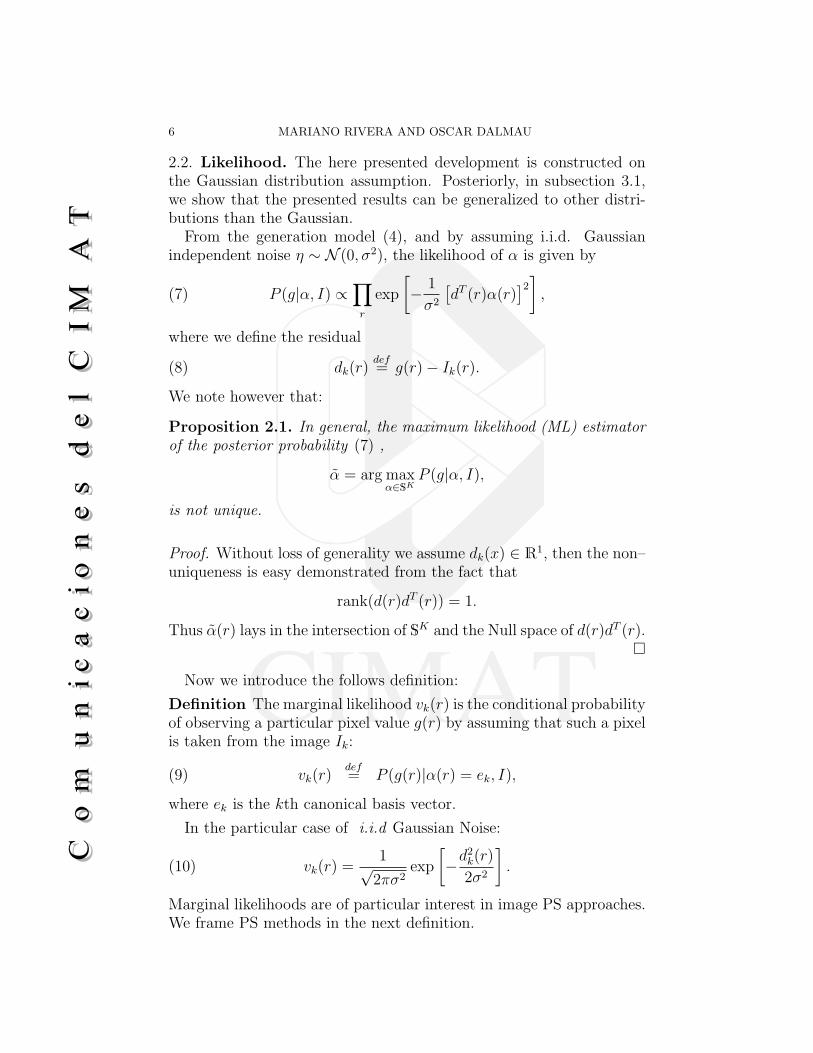
2.2. Likelihood. The here presented development is constructed onthe Gaussian distribution assumption. Posteriorly, in subsection 3.1,we show that the presented results can be generalized to other distri-butions than the Gaussian.
From the generation model (4), and by assuming i.i.d. Gaussianindependent noise " ' N (0, '2), the likelihood of ! is given by
(7) P (g|!, I) ("
r
exp
#& 1
'2
$dT (r)!(r)
%2&
,
where we define the residual
(8) dk(r)def= g(r)& Ik(r).
We note however that:
Proposition 2.1. In general, the maximum likelihood (ML) estimatorof the posterior probability (7) ,
! = arg max!!SK
P (g|!, I),
is not unique.
Proof. Without loss of generality we assume dk(x) " R1, then the non–uniqueness is easy demonstrated from the fact that
rank(d(r)dT (r)) = 1.
Thus !(r) lays in the intersection of SK and the Null space of d(r)dT (r).!
Now we introduce the follows definition:
Definition The marginal likelihood vk(r) is the conditional probabilityof observing a particular pixel value g(r) by assuming that such a pixelis taken from the image Ik:
vk(r)def= P (g(r)|!(r) = ek, I),(9)
where ek is the kth canonical basis vector.
In the particular case of i.i.d Gaussian Noise:
(10) vk(r) =1)
2('2exp
#&d2
k(r)
2'2
&.
Marginal likelihoods are of particular interest in image PS approaches.We frame PS methods in the next definition.

CONVEX QUADRATIC PROGRAMMING FOR IMAGE SEGMENTATION 7
Definition Consistence Condition Qualification (CCQ). Let v(r)be the marginal likelihood vector at pixel r, then, in absence of priorknowledge (uniform prior distributions), PS procedures compute a prob-ability measure field p, with p(r) " SK , $r, that satisfies:
(11) maxk
pk(r) = maxk
vk(r),$r.
If a vector p holds (11) we say that p is CCQ. Note that if p isCCQ w.r.t. v(r), then it is also CCQ w.r.t. the pixel-wise normalizedmarginal likelihood vk(r) = vk(r)/(1T v(r)).
Proposition 2.2. In general, the ML estimators of (7) are not CCQ.
Rather to give a rigorous proof to Proposition (2.2), we present aninformal counterexample to its contradiction: if p is a ML estimator of(7), then p is CCQ. Suppose that the observed pixel has a particularvalue, says g = 2, generated with g = (!")T m; where m = (1, 2, 3)T and!" = (0, 1, 0)T is CCQ. Then, for instance, the vector ! = (1/2, 0, 1/2)T
is also an ML estimator. However ! is not CCQ. Thus the contradictionis false.
In last example, we can note that !" is more compact (has the fewercoe"cient di!erent from zero) than any other ML estimator. Our intu-ition says that, for explaining the data, we should prefer simple modelsover complex ones: the parsimony principle. Since ! can be seen asa discrete distribution, compact representations have smallest entropy.This discussion will be useful for constraining the ML estimators of(7) for being CCQ. Following we present and discuss three candidateconstraints:
i.: Zero entropy (maxima information):
(12) !k(r)!l(r) = 0, $r,$k *= j.
This constraint (entropy equal zero) implies !k(r) " {0, 1} andresults in a hard segmentation approach. The original QMMFformulation is constructed on this constraint despite computesa soft–segmentation [1].
ii.: Zero entropy at imperfectly explained data:
(13) !k(r)!l(r) [1& vk(r)] [1& vl(r)] = 0, $r,$k *= l.
Imperfect explained pixels are those without a model with mar-ginal likelihood equal one. Thus, if we have a pixel r such that[1& vk(r)] [1& vl(r)] > 0 (for k *= l) then the entropy at sucha pixel is enforced to be equal zero, i.e. !k(r)!l(r) = 0, fork *= l. Note that 1 & vk(r) can be replaced by |dk(r)|, where
d2k(r)
def= & log vk(r), and (because of the equality constraint)
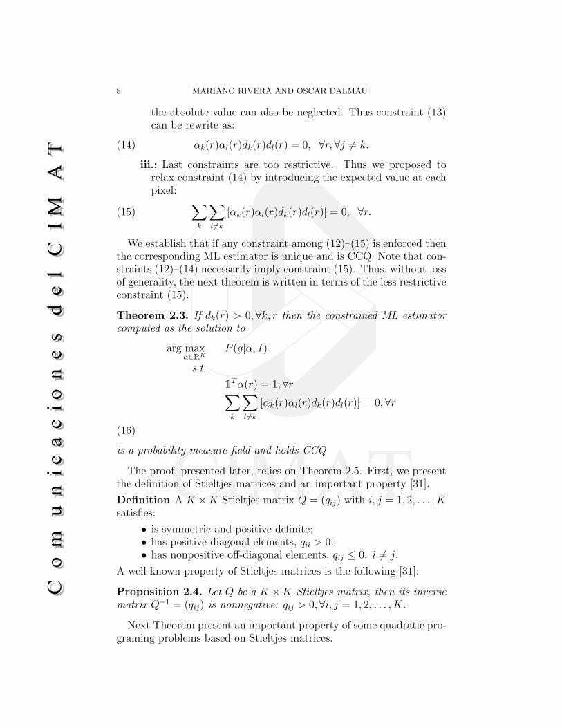
8 MARIANO RIVERA AND OSCAR DALMAU
the absolute value can also be neglected. Thus constraint (13)can be rewrite as:
(14) !k(r)!l(r)dk(r)dl(r) = 0, $r,$j *= k.
iii.: Last constraints are too restrictive. Thus we proposed torelax constraint (14) by introducing the expected value at eachpixel:
(15)!
k
!
l #=k
[!k(r)!l(r)dk(r)dl(r)] = 0, $r.
We establish that if any constraint among (12)–(15) is enforced thenthe corresponding ML estimator is unique and is CCQ. Note that con-straints (12)–(14) necessarily imply constraint (15). Thus, without lossof generality, the next theorem is written in terms of the less restrictiveconstraint (15).
Theorem 2.3. If dk(r) > 0,$k, r then the constrained ML estimatorcomputed as the solution to
arg max!!RK
P (g|!, I)
s.t.
1T !(r) = 1, $r!
k
!
l #=k
[!k(r)!l(r)dk(r)dl(r)] = 0, $r
(16)
is a probability measure field and holds CCQ
The proof, presented later, relies on Theorem 2.5. First, we presentthe definition of Stieltjes matrices and an important property [31].
Definition A K +K Stieltjes matrix Q = (qij) with i, j = 1, 2, . . . , Ksatisfies:
• is symmetric and positive definite;• has positive diagonal elements, qii > 0;• has nonpositive o!-diagonal elements, qij , 0, i *= j.
A well known property of Stieltjes matrices is the following [31]:
Proposition 2.4. Let Q be a K +K Stieltjes matrix, then its inversematrix Q$1 = (qij) is nonnegative: qij > 0,$i, j = 1, 2, . . . , K.
Next Theorem present an important property of some quadratic pro-graming problems based on Stieltjes matrices.
CONVEX QUADRATIC PROGRAMMING FOR IMAGE SEGMENTATION 9
Theorem 2.5. Let Q be a Stieltjes matrix, then the minimizer of
minx!RK
1
2xT Qx s.t. 1T x = 1(17)
holds x > 0.
Proof. The Karush-Kuhn-Tucker (KKT) conditions of (17) are
Qx& (1 = 0(18)
1T x& 1 = 0,(19)
where ( is the Lagrange’s multiplier. Then from (18):
x = (Q$11.(20)
Substituting this result in (19), we have (1T Q$11 = 1, thus
( =1
1T Q$11(21)
and using this formula into (20):
x =Q$11
1T Q$11.(22)
We can conclude that x > 0, since, from Proposition 2.4, Q$1 is positiveand thus its sums by row and over all its entries are positive; Q$11 > 0and 1T Q$11 > 0, respectively. !
In last proof we can note that the Lagrange multiplier is nonnegative[see (21)], hence we generalize last results in the next Corollary.
Corollary 2.6. Let Q be a Stieltjes matrix, then the minimizer ofminx!RK
12x
T Qx subject to 1T x # 1 holds: x > 0 and 1T x = 1.
Now we are in position to present the proof to Theorem 2.3.
Proof. (Theorem 2.3) If (15) is enforced, we have$!T (r)d(r)
%2=
!
k
[!k(r)dk(r)]2 .
Thus, because of Theorem 2.5, the ML estimator is a probability mea-sure field. Such an ML estimator is the optimizer (for all r) of theLagrangian:
min!
max#
1
2
!
k
!2k(r)d
2k(r)& ((r)
$1T !(r)& 1
%(23)
10 MARIANO RIVERA AND OSCAR DALMAU
where ( are the Lagrange’s multipliers. Since the ML estimator satisfiesthe KKT conditions:
!k(r)d2k(r) = ((r),$k
1T !(r) = 1,
we have !k(r) = ((r)/d2k(r) = ((r)/[& log vk(r)]. Given that ((r) is
a positive scalar [from (21)], we have that !k(r) is maxima for vk(r)maxima; thus the ML estimator is CCQ. !
Now that we have constrained the ML estimators to be CCQ, wepresent prior distributions for introducing special characteristics in thesegmentation. Our general prior assumes independency between mat-tings ! and images I, and a uniform distribution on the images; thenthe prior probabilities are of the form:
P (!, I) ( Ps(!)Ph(!)
where the priors Ps and Ph introduce, respectively, an explicit controlon the smoothness and on the entropy of the probability measures!(r) $r [1]. Next we discuss these particular priors.
2.3. Smoothness control prior Ps. The intra–region smoothness ispromoted by imposing a Gibbsian distribution, based on MRF models,that reduces the granularity of the regions. A popular prior form is thefirst order potential [11, 32, 33, 8, 28, 34, 1]:
(24) Ps(!) =1
Zcexp
#&$
2
!
r
!
s!Nr
%!(r)& !(s)%2wrs
&;
where Zc is a normalization constant and $ is a positive parameter thatcontrols the smoothness amount. The positive weights w are of specialinterest, they should be chosen such that wrs - 1 if the neighboringpixels r and s are likely to belong to the same class and wrs - 0 inthe opposite case. In the literature are commonly reported wights thatdepend on the magnitude of the gradient. In the task of color imagesegmentation, an instance of such weight–functions is [10, 35]:
(25) wrs =)
) + %Lab(g(r))& Lab(g(s)%2,
where Lab(·) is an operator that transforms a vector in the RGB spaceinto the Lab space. The use of the Lab-space based distance is, inthat context, motivated by its close relationship with the distance ofcolor human perception. However the Lab-space distance (as the colorhuman perceptual distance) hardly represents the inter–class (objects)distances. Inter-class distances are context and task dependent. For

CONVEX QUADRATIC PROGRAMMING FOR IMAGE SEGMENTATION 11
(a) Scribbles (b) Likelihood based (c) Color based
Figure 2. Interpixel a"nity, wrs.
instance, if the task is to segment the image in Fig. 2 into flowersand foliage, the weights should be close to zero (black) at the petalsborders. Other possibility is to segment the image into three classes:petals, foliage and headflowers; in such a case Fig. 2b shows a properweight map. As can be noted on Fig. 2c, the weights based on gradientmagnitude may not represents the intra-classes edges. Here, we proposea new inter–pixel a"nity measure based on the marginal likelihoods andthus incorporates, implicitly, the non-euclidean distances of the featurespace. Our weight proposal is
wrs =vT (r)v(x)
%v(r)%%v(s)% .(26)
Although other variants need be investigated, here we remark that:
Remark The intra–pixel a"nity wrs can be understood as the proba-bility that the neighbor pixels r, s belongs to the same class. Assumingi.i.d. samples, such a probability can be approached more preciselyfrom likelihood vectors than directly from the observed data.
Fig. 2 compares our likelihood based weights versus gradient basedones. Panel 2a shows scribbles for three classes: petals, foliage andheadflowers. Panel 2b shows the weights based on the likelihood based(26) and 2c shows the standard weights based on the image gradient(25).
2.4. Entropy control prior Ph. Entropy control steers the sharpnessof the probability measure vector at each pixel. In general, the entropycontrol prior is of the form:
Ph(!) ("
r
exp [&µH (!(r))]
where µ is a parameters that promotes entropy increment (if µ < 0) ordecrement (if µ > 0) and H(z) is an entropy measure of the discretedistribution z [36]. In order to keep quadratic the potential, in [1] is

12 MARIANO RIVERA AND OSCAR DALMAU
used the Gini’s potential as entropy measure. The Gini’s potential canbe seen the negative variance of the z values: H(z) = E2(z) & E(z2).Since E(!(r)) = 1/K, one can neglect such an !-independent term:
H(!(r)) = &!
k
!2k(r).
2.5. QMMF posterior energy and Minimization Algorithm.The posterior distribution of the matting factor ! is of the form:
P (!|g, I) ( exp [&U(!)] .
Then
Proposition 2.7. The constrained MAP estimator is computed bysolving the quadratic programing problem:
min!
U(!) s.t. !k(r) " SK , for r " %.
where the posterior energy is defined as
U(!) =!
r!R
'!
k
!2k(r)
$d2
k(r)& µ%
+$
2
!
y!Nr
%!(r)& !(s)%2wrs
(.(27)
In addition, if µ is chosen such that the energy U(!) is kept convex(i.e. d2
k(r)&µ > 0, $k, r), then the non-negativity constraints are inac-tive at the global optimal solution. In such a case, the non-negativityconstraints are neglected and thus the optimization procedure can beachieved with simple and e"cient minimization procedures for convexquadratic minimization. This is stated in next theorem.
Theorem 2.8. (Convex QMMF) Let U(!) be the energy function de-fined in (27) and assuming
lk(r; µ)def= & log vk(r)& µ > 0, $k, r;(28)
then the solution to
min!
1
2U(!) s.t. 1T !(r) = 1, for r " %
is a probability measure field.
Proof. We present an algorithmic proof to this Theorem. The optimumsolution holds the KKT conditions:
(29) !k(r)lk(r; µ) + $!
s!Nr
(!k(r)& !k(s)) wrs = ((r)

CONVEX QUADRATIC PROGRAMMING FOR IMAGE SEGMENTATION 13
(30) 1T !(r) = 1
where ( is the vector of Lagrange’s multipliers. Note that the KKTconditions are a symmetric and positive definite linear system thatcan be solved with very e"cient algorithms as Conjugate Gradient orMultigrid Gauss-Seidel (GS). In particular, a simple GS scheme resultsof integrating (29) w.r.t. k (i.e. by summing over k) and using (30):
(31) ((r) =1
K!T (r)l(r; µ).
Thus, from (29):
(32) !k(r) =ak(!, r) + ((r)
bk(r)
where we define: ak(!, r)def= $
)s!Nr
wrs!k(s) and
bk(r)def= lk(r; µ) + $
)y!Nr
wrs. Eqs. (31) and (32) define a two stepsiterative algorithm. Moreover, if (31) is substituted into (32), we cannote that if an initial positive guess for ! is chosen, then the GS scheme(32) will produce a convergent nonnegative sequence. !
One can see that the GS scheme, here proposed [Eqs. (31) and (32)],is simpler than the originally reported in [1]. In the non-convex QMMFcase we can use the projection strategy. Then at each iteration, theprojected ! can be computed with
(33) !k(r) = max
'0,
ak(!, r) + ((r)
bk(r)
(.
2.6. Binary Segmentation. The binary case (segmentation in twoclasses) is of particular interest given that many problems in computervision, image processing and image analysis require of segmenting theimage into two clases
Theorem 2.9. Convex Quadratic Markov Probability Field. Let µbe chosen such that lk(r; µ) > 0 for k = 1, 2 and $ > 0, then theunconstrained minimizer !" of the energy functional
B(!) =!
r
'!2(r)l1(r; µ) + [1& !(r)]2 l2(r; µ)
+$
2
!
y!Nr
[!(r)& !(s)]2 wrs
((34)
is a probability field, i.e. !"(r) " [0, 1].

14 MARIANO RIVERA AND OSCAR DALMAU
By defining ! = !1 and substituting !2 = 1& ! in the energy U(!)then the proof is straightforward from Theorem 2.8 . For this convexbinary case the GS scheme is given by:
(35) !(r) =l2(r) + $
)s!Nr
wrs!(s)
l1(r) + l2(r) + $)
s!Nrwrs
.
and in the non-convex binary case the projection strategy can also beused.
3. Generalizations
In this section we extend the presented QMMF formulation: otherlikelihood functions than the Gaussian, local structure information andmodel parameter estimation.
3.1. Non–Gaussian Likelihood Functions. In last section we de-rive the QMMF formulation by assuming that the image noise " is i.i.d.Gaussian. Although the Gaussianity assumption is supported by thecentral limit theorem, the use of the exact data distribution improvessignificantly the accuracy of the estimation. This is the case of mul-timode distributions as the ones empirically estimated from scribblesin an interactive segmentation approach. For removing the Gaussiannoise assumption, we first note that
Proposition 3.1. Let vk be the smooth density distribution of the pixelvalues, g(r),$r; then it can be expressed with a Gaussian mixture model[36]:
(36) vk(r) =M!
i=1
(kiGki(r),
with Gki(r)def= 1/
)2('k exp [&d2
ki(r)/2'2k], where we defined dki(r)
def=
g(r) & mki. The known parameters are denoted by &k = ('k, (k, mk);where (k " SK is the mixture coe!cients vector, mk = (mk1, mk2, . . . ,mkM)are the Gaussians’ means, 'k are the variances and M is the number(maybe very large) of Gaussians.
Thus, if we assume that such a mixture is composed by a large sum-mation of narrow Gaussians, we can state the next theorem that gener-alize of the QMMF approach for other distribution than the Gaussian:
Theorem 3.2. Let v = {vk}, for k " K, be the smooth density distribu-tions of the corresponding I = {Ik}; then the likelihood of the observed

CONVEX QUADRATIC PROGRAMMING FOR IMAGE SEGMENTATION 15
image g is given by
P (g|!, I) ="
k
"
x
#vk(r)
&!2k(r)
,(37)
if constraint (15) is provided.
The proof is presented in Appendix A.In Section 2 we derive the QMMF formulation by assuming Gaussian
marginal likelihoods. Now, by using theorem 3.2, we generalize theQMMF formulation as follows.
Proposition 3.3. Theorem 2.3 holds for other marginal likelihoods,v, than the Gaussian. Consequently the QMMF model can be usedindependently of the particular form of v.
As immediate consequence we have the next corollary.
Corollary 3.4. The QMMF model is independent of the particular
form of the negative log marginal likelihood (distance), d2k(r)
def= [ & log vk(r)].
For demonstrating last corollary, we show in the experiments a wideuse of empirical marginal likelihood functions computed with histogrammethods.
3.2. Local structured data. Frequently, the pixel color coordinates(given in a color space) are used as features for color based segmenta-tion. In contrast, in texture based segmentation the features result ofapplying a set of operators that take into account the neighborhood ofthe pixel. Instances of such operators are Gabors filters [37] and statis-tical moments [38]. The underlaying idea in statistical moments is toconsider the pixel neighborhood as samples of a (unknown) distributiondetermined by some statistics: variance, skewness, kurtosis, etc. Suchstatistics are then arrayed as a feature vector [39]. The feature vectorlength depends on the number of operators used and of the dimensionreduction technique used [40, 41]. If the generative distributions areknown (or estimated in a two step algorithm, see next subsection 3.3),then we can use an e"cient procedure for introducing texture infor-mation without the explicitly computation of texture features. Similarto statistical moments, we suppose that textured regions are gener-ated with i.i.d. random samples of particular distributions. Thus, thecontextualized marginal likelihood, V , at a pixel r should consider itsneighborhood pixels that are, almost in all the cases, generated with

16 MARIANO RIVERA AND OSCAR DALMAU
(a) Scribbles (b) " = 0 (c) " = 1 (d) " = 2
Figure 3. ML estimator for di!erent Neighborhood sizes.
the same distribution:
(38) Vk(r) ("
y!Mr
vk(s) = exp
*!
s!Mr
log vk(s)
+,
where Mr = {s : |r & s| , *} is the neighborhood of r and the pa-rameter * define the neighborhood size. Figure 3 shows MaximumLikelihood maps of (38) using di!erent neighborhood sizes, *. Notethat for large *–values the Maximum Likelihood (ML) estimator has areduced granularity but at the same time small details are lost. More-over, according with Corollary 3.4, the marginal likelihoods {Vk} arecompatible with our QMMF model.
3.3. Parameter estimation of generative models. In Ref. [1] wasstudied the particular case estimating the mean of Gaussian Likelihoodfunctions. Now, we presents the generalization of the Gaussian param-eter estimation presented in [1] to both parametric and nonparametricmodels.
In the derivation of the QMMF model we have assumed that theimage set I = {Ik} is given and thus the marginal distributions {vk}.In a generative approach such an assumption is equivalent to supposeknown the noise, ", distribution and the parameters, & = {&k}, of thegenerative models# , where Ik(r) =#( &k, r), see model (4). Fromthe posterior distribution, P (!,& |g) = 1
Z P (g|!,& )P (!,& ), we estimateboth: memberships (!) and parameters (&) by alternating partial MAPestimations:
(1) max! P (!,& |g) keeping fixed &,(2) max" P (&,! |g) keeping fixed !;

CONVEX QUADRATIC PROGRAMMING FOR IMAGE SEGMENTATION 17
until convergence. These minimization can be partially achieved asin a generalize EM scheme [42]. The maximization we concern in thissubsection is the one in the second step. This maximization is achieved
by minimizing the negative posterior energy D(!,& )def= & log P (!,& |g):
D(!,& ) =!
r
!
k
!2k(r)(& log vk(r)),(39)
where we neglect constant terms on &. Thus keeping ! fixed, the param-eters are computed by solving the system that results of."D(!,& ) = 0,where:
."kD(!,& ) =
!
r
#&!2
k(r)
vk(r)
&."k
vk(r);(40)
where ." denotes the partial gradient w.r.t. &.In the case of Gaussian Likelihood functions the update formulas
have a simple form.
Proposition 3.5. If the marginal likelihoods are Gaussians of the form
vk(r) =1)
2('k
exp
#& 1
2'2k
d2k(r)
&(41)
with dk(r) = g(r) & mk, then parameter estimation step is computedwith the formulas:
mk =
)r !2
k(r)g(r))x !2
k(r)(42)
'2k =
)r !2
k(r)(g(r)&mk)2
)r !2
k(r).(43)
The proof is presented in Appendix A. Excepting the precise def-inition of the weight, !2
k(r), formulas (42) and (43) are similar tothose used in the Expectation-Maximization (EM) procedure. Theclass mean, mk, computed with (42) can be understood as the mean ofthe data contributions to each class, k. Such contributions correspondto the normalized !2
k(r). Then non-parametric representations of like-lihood functions require of considering such data contributions. Forinstance, we generalize QMMF to histogram based likelihood functionsby weighting each pixel value with !2 at the time of computing the his-tograms. Experiments that demonstrate this procedure are presentedin subsection 4.3.
18 MARIANO RIVERA AND OSCAR DALMAU
(a) (b) (c) (d) (e)
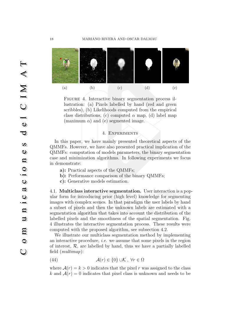
Figure 4. Interactive binary segmentation process il-lustration: (a) Pixels labelled by hand (red and greenscribbles), (b) Likelihoods computed from the empiricalclass distributions, (c) computed ! map, (d) label map(maximum !) and (e) segmented image.
4. Experiments
In this paper, we have mainly presented theoretical aspects of theQMMFs. However, we have also presented practical implication of theQMMFs: computation of models parameters, the binary segmentationcase and minimization algorithms. In following experiments we focusin demonstrate:
a): Practical aspects of the QMMFs;b): Performance comparison of the binary QMMFs;c): Generative models estimation.
4.1. Multiclass interactive segmentation. User interaction is a pop-ular form for introducing prior (high level) knowledge for segmentingimages with complex scenes. In that paradigm the user labels by handa subset of pixels and then the unknown labels are estimated with asegmentation algorithm that takes into account the distribution of thelabelled pixels and the smoothness of the spatial segmentation. Fig.4 illustrates the interactive segmentation process. These results werecomputed with the proposed algorithm, see subsection 4.2.
We illustrate our multiclass segmentation method by implementingan interactive procedure, i.e. we assume that some pixels in the regionof interest, R, are labelled by hand, thus we have a partially labelledfield (multimap):
(44) A(r) " {0} /K , $r " %
where A(r) = k > 0 indicates that the pixel r was assigned to the classk and A(r) = 0 indicates that pixel class is unknown and needs to be

CONVEX QUADRATIC PROGRAMMING FOR IMAGE SEGMENTATION 19
(a) 10 (b) 20 (c) 50 (d) 100
Figure 5. Partial solutions (segmentations) for di!er-ent iteration numbers.
estimated. If we assume correct user’s labels , then the sum on thedata term in (34) is replaced by:
!
r:A(r)=0
!
k
!2k(r)(& log vk(r)).(45)
On the other hand, by leaving the sum for all pixels r " R we assumeuncertainty in the hand labeled data.
Let g an image such that g(r) " t, with t = {t1, t2, . . . , tT} the pixelvalues (maybe vectorial values as in the case of color images), then thedensity distribution for the classes are empirically estimated by usinga histogram technique. That is, if Hki is the number of hand labelledpixels with value ti for the class k [25] then h is the smoothed histogramversion. We implement the smoothing operator by a homogeneousdi!usion process. Thus the normalized histograms are computed withhki = hki/
)l hkl and the likelihood of the pixel r to a given class k
(likelihood function, LF) is computed with:
(46) LFki =hki + +
)j(hji + +)
, $k;
with + = 1+10$8, a small constant. Thus the likelihood of an observedpixel value is computed with vk(r) = LFki such that i = minj %g(r)&tj%2. In the experiment of Fig. 5 we used the proposed likelihood com-putation (with * = 1), the inter–pixel a"nity measure (26) and the twostep GS scheme, Eqs. (31) and (32). The shown sequence correspondsto partial solutions computed with di!erent iteration number.

20 MARIANO RIVERA AND OSCAR DALMAU
(a) Original (b) Trimap
(c) GraphCut (d) QMMF+EC
Figure 6. Segmentation example from the Lasso’s data set.
4.2. Quantitative Comparisson: Image Binary Interactive Seg-mentation. Following we resume our results of a quantitative studyon the performance of the segmentation algorithms: the proposed Bi-nary variant of QMMF, the maximum flow (minimum graph cut, GC),GMMF and Random Walker (RW). The reader can found more detailsabout this study in our technical report [26]. The task is to segmentinto background and foreground (binary segmentation) color imagesallowing interactive data labeling. The generalization capabilities ofthe methods are compared with a cross-validation procedure [36]. Thecomparison was conducted on the Lasso benchmark database [8]; a setof 50 images online available [43]. Such a database contains a natu-ral image set with their corresponding trimaps and the ground truthsegmentations.
We opted to compute the weights using the standard formula (25),in order to focus our comparison on the data term of the di!erentalgorithms: QMMF, GC, GMMF and RW. In this task, empirical like-lihoods are computed from the histogram of the labeled by hand pixels[10].

CONVEX QUADRATIC PROGRAMMING FOR IMAGE SEGMENTATION 21
Table 1. Adjusted parameters for the results in table 2.
Parameter QMMF QMMF+EC
# 4.7+ 103 2.28+ 105
$ 9.14+ 10$6 5.75+ 10$3
µ 0.0 &5.75+ 105
Table 2. Cross-validation results: Parameters, Akaike in-formation criterion, training and testing error.
Algorithm Params. AIC Training TestingGraph Cut #,$ 8.58 6.82% 6.93%Rand. Walk. #,$ 6.50 5.46% 5.50%GMMF #,$ 6.49 5.46% 5.49%QMMF #,$ 6.04 5.02% 5.15%QMMF+EC #, $, µ 3.58 3.13% 3.13%
The hyper parameters ($, µ,) ) were trained by minimizing the meanof the segmentation error in the image set by using the Nelder and Meadsimplex descent [44]. We implement a cross–validation procedure fol-lowing the recommendation in Ref. [36] and split the data set into5 groups, 10 images per set. The learned parameters are reported inTable 1. Figure 6 shows an example of the segmented images. Table2 shows the resume of the training and testing error and the Akaikeinformation criterion (AIC) [36]. The AIC was computed for the opti-mized (trained) parameters with the 50 image in the database. Notethat the AIC is consistent with the cross-validation results: the order ofthe method performance is preserved. Moreover the QMMF algorithmhas the best performance in the group. Its important to note that ourGC based segmentation improves significantly the reported results in[8].
We remark that the learned parameter µ for controlling the entropy(version QMMF+EC) promotes large entropy, such a parameter wasappropriated for the trimap segmentation task and should not producethe expected results in other tasks. However the entropy control allowsone to adapt the algorithm for di!erent tasks, for instance for the caseof simultaneously estimation of segmentation and model parameters,see subsection 3.3. The e!ect of the entropy control is illustrated inFigs. 7 and 8. The QMMF method algorithm produces, in all thecases, better segmentation with smooth boundaries than GMMF, RWand GC. In particular the matting factor shown Fig. 1 was computedwith QMMF using µ = 0.

22 MARIANO RIVERA AND OSCAR DALMAU
(a) QMMF µ = 10. (b) µ = 0. (c) µ = &123.
(d) GMMF. (e) Rand. Walk. (f) GraphCut.
Figure 7. First row, results computed with the pro-posed method with a) low-entropy, b) without entropycontrol and c) high entropy. Second row, results com-puted with methods of the state of the art.
Figure 8. Label maps corresponding to Fig. 7, same order.
4.3. Robust model parameter estimation. In parametric segmen-tation, the computation of the exact Gaussian parameters is as im-portant as the robustness to noise. Figure 9 shows the results whenthe regions are generated by i.i.d. samples of Gaussian distribution:N (0, 0.92) and N (0.5, 0.92) (see also experiments in our technical re-port [26]) At this SNR, the solution computed with GC, GMMF and
CONVEX QUADRATIC PROGRAMMING FOR IMAGE SEGMENTATION 23
(a) (b) (c)
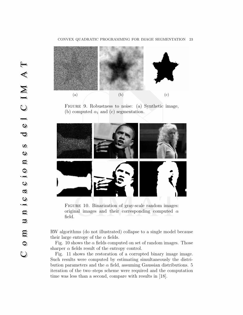
Figure 9. Robustness to noise: (a) Synthetic image,(b) computed !1 and (c) segmentation.
Figure 10. Binarization of gray-scale random images:original images and their corresponding computed !field.
RW algorithms (do not illustrated) collapse to a single model becausetheir large entropy of the ! fields.
Fig. 10 shows the ! fields computed on set of random images. Thosesharper ! fields result of the entropy control.
Fig. 11 shows the restoration of a corrupted binary image image.Such results were computed by estimating simultaneously the distri-bution parameters and the ! field, assuming Gaussian distributions. 5iteration of the two–steps scheme were required and the computationtime was less than a second, compare with results in [18].

24 MARIANO RIVERA AND OSCAR DALMAU
(a) (b) (c)
Figure 11. Binary restoration: a) Iceland corruptedmap, b) computed ! and c) segmentation.
In all the cases shown in Figs. 9, 10 and 11 implementations basedon Gauss Markov Measure Fields (GMMF, an early variant of RandomWalker [7]) collapsed to a single model [5]. That limitation of theGMMF model is discussed in [45], see also [26].
Finally, Fig. 12 demonstrates generalization of the QMMFs forcomputing LF based on histogram techniques. The histograms arecomputed by !2–weighting the pixel values, we initially set !k(r) =vk(r),$k, r. The erroneous segmentation at the first iteration is prod-uct of inaccurate scribbles and thus inaccurate initial LF (class his-tograms). The segmentation after two iteration demonstrates the abil-ity of the QMMFs for estimating nonparametric class distributions.
5. Conclusions and Discussion
We presented a derivation of the QMMF model that relax signif-icantly the minimal entropy constraint. Therefore, based on priorknowledge, we can control the amount of entropy increment, or decre-ment, in the computed probability measures. We demonstrated thatthe QMMF models are general and accept any marginal probabilityfunctions. As demonstration of such a generalization we presented ex-periments with iterative estimation of likelihood functions based onhistogram techniques. We proposed robust likelihoods that improvethe method performance for segmenting textured regions.
Our contributions in this work are mainly theoretical extensions andgeneralization to the QMMF model. Along the paper we present aseries of experiments for demonstrating our proposals. Additionally,we present an experimental comparison with respect algorithms of thestate of the art. We selected the task of binary interactive segmen-tation for conducting our comparison, first because it demonstrates

CONVEX QUADRATIC PROGRAMMING FOR IMAGE SEGMENTATION 25
Figure 12. Iterative estimation of empirical likelihoodfunctions by histograms of !2–weighted data. Binarysegmentation: initial scribbles, first iteration and seconditeration; respective columns.
the use of the entropy control in the case of generic likelihood func-tions. Second, a benchmark database is online available, and finallyour hyper–parameter training scheme demonstrates to be objective by,significantly, improving the previously reported results with a graphcut based method.
6
Proof for Theorem 3.2. According to the generation model (7) and us-ing (15), we have:
P (g|!, I) ("
k
"
r
' M!
i=1
(ki)2('k
exp
#&d2
ki(r)!2k(r)
2'2k
&(
="
k
"
r
' M!
i=1
(ki [Gki(r)]!2
k(r)
(.(47)
Then, assuming narrow Gaussians and a large number, M , of them:
(48) limM%&,$k%0
Gki(r)Gkj(r) = 0; i *= j, $k

26 MARIANO RIVERA AND OSCAR DALMAU
if mki *= mkj is provided. Thus, in the limitM!
i=1
(ki [Gki(r)]!2
k(r) =
# M!
i=1
(kiGki(r)
&!2k(r)
=
#vk(r)
&!2k(r)
.(49)
Then (37) results of substituting (49) into (47). !Proof for Proposition 3.5. The result is proved if we substitute in (40)the partial derivatives:
,D
,mk=
1
'2k
dk(r)vk(r),
,D
,'k=
#1
'2k
d2k(r)&
1
'i
&vi(r).
Then, we solve for mk and '2k the system ."D(!,& ) = 0. !

CONVEX QUADRATIC PROGRAMMING FOR IMAGE SEGMENTATION 27
References
[1] M. Rivera, O. Ocegueda, and J. L. Marroquin, “Entropy-controlled quadraticMarkov measure field models for e!cient image segmentation,” IEEE Trans.Image Processing, vol. 8, no. 12, pp. 3047–3057, Dec. 2007.
[2] S. Z. Li, Markov Random Field Modeling in Image Analysis. Springer-Verlag,Tokyo, 2001.
[3] J. Besag, “On the statistical analisys of dirty pictures,” J. R. Stat. Soc., Ser.B, Methodol., vol. 48, pp. 259–302, 1986.
[4] S. Geman and D. Geman, “Stochastic relaxation, Gibbs distribution and theBayesian restoration of images,” IEEE PAMI, vol. 6, no. 6, pp. 721–741, 1984.
[5] J. L. Marroquin, F. Velazco, M. Rivera, and M. Nakamura, “Probabilisticsolution of ill–posed problems in computational vision,” IEEE Trans. PatternAnal. Machine Intell., vol. 23, pp. 337–348, 2001.
[6] V. Kolmogorov and R. Zabih, “What energy functions can be minimized viagraph cuts,” in European Conference on Computer Vision (ECCV02)., 2002.
[7] L. Grady, “Random walks for image segmentation,” IEEE Trans. PatternAnal. Mach. Intell., vol. 28, no. 11, pp. 1768–1783, 2006.
[8] A. Blake, C. Rother, M. Brown, P. Perez, and P. Torr, “Interactive imagesegmentation using an adaptive GMMRF model,” in ECCV, vol. 1, 2004, pp.414–427.
[9] C. A. Bouman and M. Shapiro, “A multiscale random field model for bayesianimage segmentation,” IEEE Trans. Image Processing, vol. 3, no. 2, pp. 162–177, 1994.
[10] Y. Boykov and M.-P. Jolly, “Interactive graph cut for optimal boundary ®ion segmentation of objects in N–D images,” in ICIP (1), 2001, pp. 105–112.
[11] Y. Boykov, O. Veksler, and R. Zabih, “Fast approximate energy minimizationvia graph cuts,” IEEE Trans. Pattern Anal. Machine Intell., vol. 23, no. 11,pp. 1222–1239, 2001.
[12] S. Geman and D. Geman, “Stochastic relaxation, Gibbs distributions andBayesian restoration of images,” IEEE Trans. Pattern Anal. Machine Intell.,vol. 6, pp. 721–741, 1984.
[13] O. Juan and R. Keriven, “Trimap segmentation for fast and user-friendly alphamatting,” in VLSM, LNCS 3752, 2005, pp. 186–197.
[14] V. Kolmogorov, A. Criminisi, A. Blake, G. Cross, and C. Rother, “Probabilisticfusion of stereo with color and contrast for bi-layer segmentation,” IEEE Trans.Pattern Anal. Mach. Intell., vol. 28, no. 9, pp. 1480–1492, 2006.
[15] C. Rother, V. Kolmogorov, and A. Blake, “Interactive foreground extractionusing iterated graph cuts,” in ACM Transactions on Graphics, no. 23 (3), 2004,pp. 309–314.
[16] Y. Weiss, “Segmentation using eigenvectors: A unifying view,” in ICCV (2),1999, pp. 975–982.
[17] J. Shi and J. Malik, “Normalized cuts and image segmentation,” IEEE Trans.Pattern Anal. Machine Intell., vol. 22, no. 8, pp. 888–905, 2000.
[18] C. Olsson, A. P. Eriksson, and F. Kahl, “Improved spectral relaxation meth-ods for binary quadratic optimization problems,” Computer Vision and ImageUnderstanding, vol. 112, pp. 30–38, 2008.

28 MARIANO RIVERA AND OSCAR DALMAU
[19] N. Komodakis, G. Tziritas, and N. Paragios, “Performance vs computationale!ciency for optimizing single and dynamic MRFs: Setting the state of theart with primal–dual strategies,” Computer Vision and Image Understanding,vol. 112, pp. 14–29, 2008.
[20] P. Kohli and P. H. S. Torr, “Measuring uncertainty in graph cut solutions,”Computer Vision and Image Understanding, vol. 112, pp. 30–38, 2008.
[21] M. Rivera, O. Ocegueda, and J. L. Marroquin, “Entropy controlled Gauss-Markov random measure fields for early vision,” in VLSM, vol. LNCS 3752,2005, pp. 137–148.
[22] A. Levin, A. Rav-Acha, and D. Lischinski, “Spectral matting,” IEEE Trans.Pattern Anal. Mach. Intell., vol. 30, no. 10, pp. 1–14, 2008.
[23] J. Nocedal and S. J. Wright, Numerical Optimization. Springer Series inOperation Research, 2000.
[24] W. L. Briggs, S. McCormick, and V. Henson, A Multigrid Tutorial, 2nd ed.SIAM Publications, 2000.
[25] M. Rivera and P. P. Mayorga, “Quadratic markovian probability fields forimage binary segmentation,” in in Proc. ICCV, Workshop ICV 07, 2007, pp.1–8.
[26] ——, “Comparative study on quadratic Markovian probability fields for imagebinary segmentation,” CIMAT A.C., Mexico, Tech. Rep. 10.12.2007, I-07-15(CC), December 2007.
[27] M. Rivera, O. Dalmau, and J. Tago, “Image segmentation by convex quadraticprogramming,” in Int. Conf. on Pattern Recognition (ICPR08), 2008.
[28] L. Grady, “Computing exact discrete minimal surfaces: Extending and solvingthe shortest path problem in 3D with application to segmentation,” in CVPR(1), June 2006, pp. 69–78.
[29] O. Dalmau, M. Rivera, and P. P. Mayorga, “Computing the alpha–channelwith probabilistic segmentation for image colorization,” in in Proc. ICCV,Workshop ICV 07, 2007, pp. 1–7.
[30] P. Kohli and P. H. S. Torr, “Dynamic graph cuts for e!cient inference inMarkov random fields,” IEEE Trans. Pattern Anal. Mach. Intell., vol. 29,no. 12, pp. 2079–2088, 2007.
[31] R. S. Varga, Matrix Iterative Analysis, 2nd ed. Springer Series in Computa-tional Mathematics, 2000, vol. 27.
[32] Y. Boykov and V. Kolmogorov, “An experimental comparison of min-cut/max-flow algorithms for energy minimization in vision,” Int’l J. Computer Vision,vol. 70, no. 2, pp. 109–131, 2006.
[33] A. Levin, D. Lischinski, and Y. Weiss, “Colorization using optimization,” ACMTrans. Graph., vol. 23, no. 3, pp. 689–694, 2004.
[34] S. Kumar and M. Hebert, “Discriminative random fields,” Int’l J. ComputerVision, vol. 68, no. 2, pp. 179–201, 2006.
[35] L. Grady, Y. Sun, and J. Williams, “Interactive graph-based segmentationmethods in cardiovascular imaging,” in Handbook of Mathematical Models inComputer Vision, N. P. et al., Ed. Springer, 2006, pp. 453–469.
[36] T. Hastie, R. Tibshirani, and J. Friedman, The elements of statistical learning.Springer, 2001.
[37] A. K. Jain and F. Farrokhnia, “Unsupervised texture segmentation using gaborfilters,” Pattern Recogn., vol. 24, no. 12, pp. 1167–1186, 1991.

CONVEX QUADRATIC PROGRAMMING FOR IMAGE SEGMENTATION 29
[38] M. Tuceryan, “Moment based texture segmentation,” Pattern Recognition Let-ters, vol. 15, pp. 659–668, 1994.
[39] S. Belongie, C. Carson, H. Greenspan, and J. Malik, “Color- and texture-based image segmentation using em and its application to content-based imageretrieval,” in ICCV’98, 1998, pp. 675–682.
[40] D. A. Clausi and H. Deng, “Design-based texture feature fusion using gaborfilters and co-occurrence probabilities,” IEEE Trans. Image Processing, vol. 14,no. 7, pp. 925–936, 2005.
[41] J. Ramirez-Ortegon and M. Rivera, “Probabilistic rules for automatic texturesegmentation,” in Proc MICAI 2006, vol. LNAI 4293. Springer, 2006, pp.778–788.
[42] R. M. Neal and G. E. Hinton, “A view of the EM algorithm that justifiesincremental, sparse, and other variants,” in Learning in Graphical Models,M. I. Jordan, Ed. Kluwer Academic Publishers, Boston MA., 1998, pp. 355–368.
[43] http://research.microsoft.com/vision/cambridge/i3l/segmentation/GrabCut.htm.
[44] J. A. Nelder and R. Mead, “A simplex method for function minimization,”Comput. J., vol. 7, pp. 308–313, 1965.
[45] J. L. Marroquin, B. C. Vemuri, S. Botello, F. Calderon, and A. Fernandez-Bouzas, “An accurate and e!cient Bayesian method for automatic segmen-tation of brain MRI,” IEEE Trans. Medical Imaging, vol. 21, pp. 934–945,2002.