Rom. Journ. Phys., Vol. 54, Nos. 9–10 , P. 823–832, Bucharest, 2009

SOLVING OF THE FRACTIONAL NON-LINEAR

AND LINEAR SCHRÖDINGER EQUATIONS

BY HOMOTOPY PERTURBATION METHOD

DUMITRU BALEANU1, ALIREZA K. GOLMANKHANEH2,3, ALI K. GOLMANKHANEH3

1 Department of Mathematics and Computer Science, Çankaya University, 06530 Ankara, Turkey

and Institute of Space Sciences, P.O. BOX, MG-23, RO-077125, Mãgurele – Bucharest, Romania,

E-mail: dumitru@cankaya.edu.tr2 Department of Physics, University of Pune, Pune, 411007, India

E-mail: alireza@physics.unipune.ernet.in3 Department of Physics, Islamic Azad University-Uromia Branch, PO Box 969, Uromia, Iran

E-mail: ali.khalili.gol@gmail.com

Received December 28, 2008

In this paper, the homotopy perturbation method is applied to obtain

approximate analytical solutions of the fractional non-linear Schrödinger equations.

The solutions are obtained in the form of rapidly convergent infinite series with

easily computable terms. We illustrated the ability of the method for solving

fractional non linear equation by some examples.

1. INTRODUCTION

The theory of fractional calculus goes back to Leibniz, Liouville, Riemann,

Grunwald and Letnikov has been found many application in science and

engineering [1–7]. Finding accurate and efficient methods for solving fractional

non-linear differential equations (FNLDEs) has been an active research

undertaking. Exact solutions of most of the FNLDEs can not be found

easily, thus analytical and numerical methods must be used. The Adomian

Decomposition Method (ADM) was shown to be applicable to linear and

nonlinear fractional differential equations [8]. However, another analytic technique

for nonlinear problems is called the homotopy perturbation method, first

proposed by He [9–14]. In refs [15, 16] homotopy perturbation method is used to

solve linear and nonlinear fractional differential equations. The solution of the

Schrödinger equation over an infinite integration interval by perturbation

methods was given in [17]. Recently, in [18] an analytical approximation to the

solution of Schrödinger equations has been obtained. Very recently, analytical

and approximate solutions for different nonlinear Schrödinger equation of

fractional (NLSF) order involving Caputo derivatives has been obtained by

Adomian Decomposition Method [19]. In the present, we obtain the analytical

824 D. Baleanu, A. K. Golmankhaneh, Ali K. Golmankhaneh 2

and approximate solutions for fractional nonlinear Schrödinger equation using

homotopy perturbation method. The plan of the paper is as follows:

Section 2 is dedicated to the notion of fractional integral and fractional

derivatives. Section 3 contains a brief summary of homotopy perturbation

method. Section 4 deals with using homotopy perturbation method for solving

fractional nonlinear Schrödinger equation. Finally, Section 5 provides some

examples for illustrating of the ability of method.

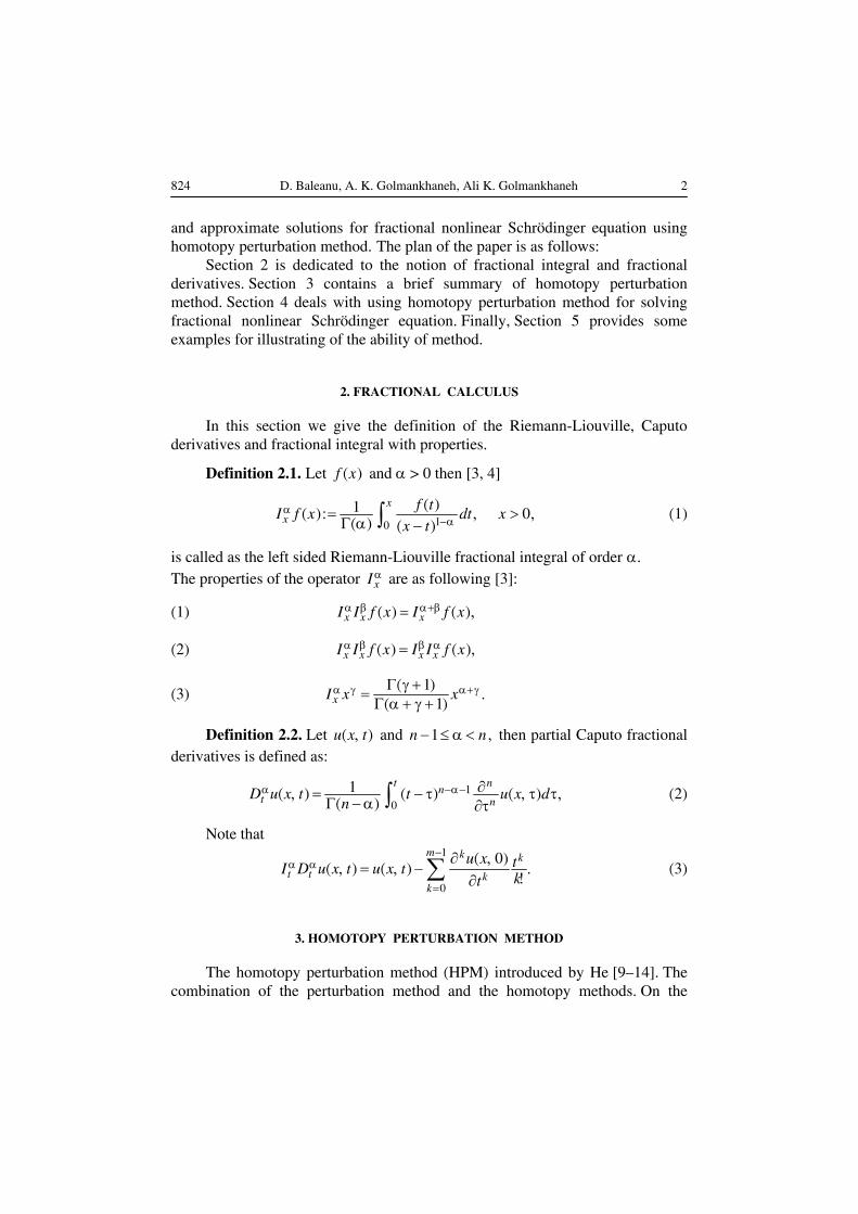
2. FRACTIONAL CALCULUS

In this section we give the definition of the Riemann-Liouville, Caputo

derivatives and fractional integral with properties.

Definition 2.1. Let ( )f x and > 0 then [3, 4]

10

( )1( ) 0( ) ( )

x

x

f tI f x dt x

x t

(1)

is called as the left sided Riemann-Liouville fractional integral of order .

The properties of the operator xI are as following [3]:

(1) ( ) ( )x x xI I f x I f x

(2) ( ) ( )x x x xI I f x I I f x

(3)( 1)

( 1)xI x x

Definition 2.2. Let ( )u x t and 1 ,n n then partial Caputo fractional

derivatives is defined as:

1

0

1( ) ( ) ( )( )

t nn

t nD u x t t u x d

n

(2)

Note that1

0

( 0)( ) ( )

m k k

t t kk

u x tI D u x t u x tkt

(3)

3. HOMOTOPY PERTURBATION METHOD

The homotopy perturbation method (HPM) introduced by He [9–14]. The

combination of the perturbation method and the homotopy methods. On the

3 Solving of the fractional non-linear and linear Schrödinger equations 825

other hand, this technique can have full advantage of the traditional perturbation

techniques. In this method the solution is considered as the summation of an

infinite series which usually converges rapidly to the exact solutions. In this

section, basic ideas of this method has been explained.

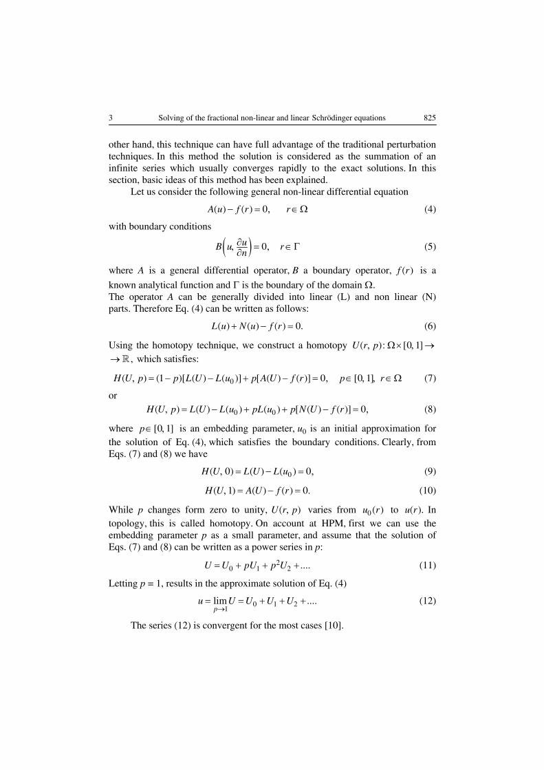
Let us consider the following general non-linear differential equation

( ) ( ) 0A u f r r (4)

with boundary conditions

0uB u rn

(5)

where A is a general differential operator, B a boundary operator, ( )f r is a

known analytical function and is the boundary of the domain .

The operator A can be generally divided into linear (L) and non linear (N)

parts. Therefore Eq. (4) can be written as follows:

( ) ( ) ( ) 0L u N u f r (6)

Using the homotopy technique, we construct a homotopy ( ) [0 1]U r p , which satisfies:

0( ) (1 )[ ( ) ( )] [ ( ) ( )] 0 [0 1]H U p p L U L u p A U f r p r (7)

or

0 0( ) ( ) ( ) ( ) [ ( ) ( )] 0H U p L U L u pL u p N U f r (8)

where [0 1]p is an embedding parameter, u0 is an initial approximation for

the solution of Eq. (4), which satisfies the boundary conditions. Clearly, from

Eqs. (7) and (8) we have

0( 0) ( ) ( ) 0H U L U L u (9)

( 1) ( ) ( ) 0H U A U f r (10)

While p changes form zero to unity, ( )U r p varies from 0 ( )u r to ( ).u r In

topology, this is called homotopy. On account at HPM, first we can use the

embedding parameter p as a small parameter, and assume that the solution of

Eqs. (7) and (8) can be written as a power series in p:

20 1 2U U pU p U (11)

Letting p = 1, results in the approximate solution of Eq. (4)

0 1 21

limp

u U U U U

(12)

The series (12) is convergent for the most cases [10].

826 D. Baleanu, A. K. Golmankhaneh, Ali K. Golmankhaneh 4

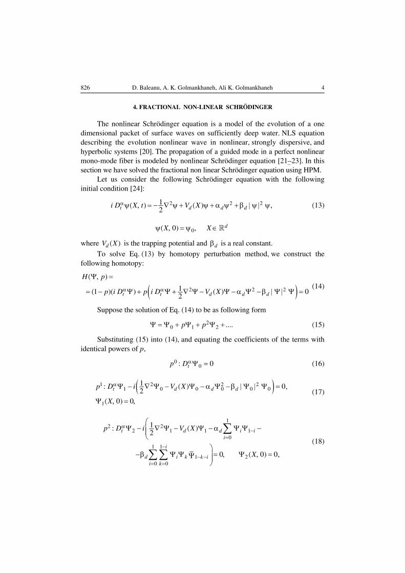
4. FRACTIONAL NON-LINEAR SCHRÖDINGER

The nonlinear Schrödinger equation is a model of the evolution of a one

dimensional packet of surface waves on sufficiently deep water. NLS equation

describing the evolution nonlinear wave in nonlinear, strongly dispersive, and

hyperbolic systems [20]. The propagation of a guided mode in a perfect nonlinear

mono-mode fiber is modeled by nonlinear Schrödinger equation [21–23]. In this

section we have solved the fractional non linear Schrödinger equation using HPM.

Let us consider the following Schrödinger equation with the following

initial condition [24]:

2 2 21( ) ( )2t d d di D X t V X (13)

0( 0) dX X

where ( )dV X is the trapping potential and d is a real constant.

To solve Eq. (13) by homotopy perturbation method, we construct the

following homotopy:

2 2 2

( )

1(1 )( ) ( ) 02t t d d d

H p

p i D p i D V X

(14)

Suppose the solution of Eq. (14) to be as following form

20 1 2p p (15)

Substituting (15) into (14), and equating the coefficients of the terms with

identical powers of p,

00 0tp D (16)

1 2 2 21 0 0 0 0 0

1

1 ( ) 02

( 0) 0

t d d dp D i V X

X

(17)

12 2

2 1 1 1

0

1 1

21

0 0

1 ( )2

0 ( 0) 0

t d d i i

i

i

d i k k i

i k

p D i V X

X

(18)

5 Solving of the fractional non-linear and linear Schrödinger equations 827

23 2

3 2 2 2

0

2 2

2 3

0 0

1 ( )2

0 ( 0) 0

t d d i i

i

i

d i k k i

i k

p D i V X

X

(19)

12

1 1

0

1

0 0

1 ( )2

0 ( 0) 0

jj

t j j d j d i j i i

i

j j i i

d i k j k i j

i k

p D i V X

X

(20)

where in ,jp there are the multiplication of two series 2 and .

For simplicity we take

0 0 ( 0)X (21)

Having this assumption we get the following iterative equation

11 2

1 10

0

1 1

0 0

1( ) ( )( ) 2

jt

j j d j d i j i i

i

j j i

d i k j k i

i k

i t V X

d

(22)

The approximate solution of (13) can be obtained by setting p = 1,

0 1 21

limp

5. EXAMPLES

We have used HPM for solving following example for efficiency of the

method in fractional nonlinear and linear equation.

828 D. Baleanu, A. K. Golmankhaneh, Ali K. Golmankhaneh 6

5.1. EXAMPLE 1

Consider the following one dimensional Schrödinger equation with the

following initial condition [25].

22

2

1( ) 02ti D x t t

x

(23)

( 0) ixx e

He’s homotopy perturbation method consists of the following scheme

22

2

1( ) (1 ) 02t tH p p i D p i D

x

(24)

Starting with 0 0 ( 0) ,ixx e using (22) we obtain the recurrence

relation

1 1211

200 0

1( ) 1 2 3( ) 2

j j it j

j i k j k i

i k

i t d jx

(25)

The solution reads

1( )2 ( 1)

ixitx t e

2

2 ( )4 (2 1)

ixtx t e

3

3( )8 (3 1)

ixitx t e

General form can be written as

( )( )

2 ( 1)

nix

n n

itx t e

n

Finally, solution will be as

10

( )( ) lim ( )

2 ( 1)

nix

npn

itx t x t e

n

7 Solving of the fractional non-linear and linear Schrödinger equations 829

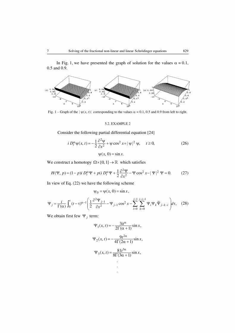
In Fig. 1, we have presented the graph of solution for the values = 0.1,

0.5 and 0.9.

Fig. 1 – Graph of the ( )x t corresponding to the values = 0.1, 0.5 and 0.9 from left to right.

5.2. EXAMPLE 2

Consider the following partial differential equation [24]

22 2

2

1( ) cos 02ti D x t x t

x

(26)

( 0) sinx x

We construct a homotopy [0 1] which satisfies

22 2

2

1( ) (1 ) ( cos 02t tH p p i D p i D x

x

(27)

In view of Eq. (22) we have the following scheme

0 ( 0) sin ,x x

1 1211 2

1200 0

1( ) cos( ) 2

j j it j

j j i k j k i

i k

i t x dx

(28)

We obtain first few j term:

13( ) sin

2 ( 1)itx t x

2

29( ) sin

4 (2 1)tx t x

3

381( ) sin

8 (3 1)tx t x

830 D. Baleanu, A. K. Golmankhaneh, Ali K. Golmankhaneh 8

Thus, solution will be as:

10

( 3 )( ) lim ( ) sin

2 ( 1)

n

npn

itx t x t x

n

5.3. EXAMPLE 3

Consider linear Schrödinger equation as following

2

2( ) 0ti D x t i

x

(29)

with initial condition

( 0) 1 sinh(2 )x x

Let construct the following homotopy:

2

2( ) (1 ) ( ) ( ) 0t tH p p i D x t p i D x t i

x

(30)

Substituting from Eq. (15) into Eq. (30), rearranging based on powers of

p-terms and solving the resulted equations, we have:

0 ( ) 1 sinh(2 )x t x

14( ) sinh(2 )

( 1)itx t x

( 4 )( ) sinh(2 )

( 1)

n

n

itx t x

n

The solution of the Eq. (29) when 1p will be as follows:

11

( 4 )( ) lim ( ) 1 sinh(2 )

( 1)

n

pn

itx t x t x

n

5.4. EXAMPLE 4

Consider the following three dimensional Schrödinger equation with the

following initial condition [24]

9 Solving of the fractional non-linear and linear Schrödinger equations 831

2 2 22

2 2 2

1( ) ( )2

0 ( ) [0 2 ] [0 2 ] [0 2 ]

ti D x t V x y zx y z

t x y z

(31)

( 0) sin sin sinx y z x y z

where 2 2 2( ) 1 sin sin sin .V x y z x y z We construct a homotopy [0 1] which satisfies

2 2 2

2 2 2

2

1( ) (1 ) ( )2

( ) 0

t tH p p i D x t p iDx y z

V x y z

(32)

In virtue of Eq. (22) we get the recurrence relation

0 0 ( 0) sin sin sinx y z x y z

2 2 21 1 11

2 2 20

1 1

1

0 0

1( )( ) 2

( ) )

t j j jj

j j i

j i k j k i

i k

i tx y z

V x y z d

(33)

We derive the following results

15( ) sin sin sin

2 ( 1)itx y z t x y z

2

225( ) sin sin sin

4 (2 1)tx y z t x y z

3

325( ) sin sin sin

8 (3 1)itx y z t x y z

( 5 )( ) sin sin

2 ( 1)

n

n n

itx y z t x y

n

832 D. Baleanu, A. K. Golmankhaneh, Ali K. Golmankhaneh 10

Solution of Eq. (31) will be derived by these terms, so

10

( 5 )( ) lim ( ) sin sin sin

2 ( 1)

n

npn

itx y z t x t x y z

n

6. CONCLUSION

In the present paper we obtain analytical approximate solution for fractional

nonlinear Schrödinger equation by homotopy perturbation method it shows that

ability of the homotopy perturbation method in nonlinear fractional equation.

REFERENCES

1. K. B. Oldham, J. Spanier, The Fractional Calculus, Academic Press, 1974.

2. K. S. Miller, B. Ross, An Introduction to the Fractional Integrals and Derivatives – Theory

and Application, John Wiley and Sons, 1993.

3. S. G. Samko, A. A. Kilbas, O. I. Marichev, Fractional Integrals and Derivatives – Theory and

Applications, Gordon and Breach, 1993.

4. R. Hilfer, Applications of Fractional Calculus in Physics, World Scientific, 2000.

5. I. Podlubny, Fractional Differential Equations, Academic Press, 1999.

6. G. M. Zaslavsky, Hamiltonian Chaos and Fractional Dynamics, Oxford University Press, 2005.

7. A. A. Kilbas, H. M. Srivastava, J. J. Trujillo, Theory and Applications of Fractional

Differential Equations, Elsevier, 2006.

8. V. Daftardar-Gejji, H. Jafari, J. Math. Anal., 301, 508 (2005).

9. J. H. He, Comput. Mathods Appl. Mech. Engrg., 178, 257 (1999).

10. J. H. He, Int. J. Non-Linear Mech., 35, 37 (2000).

11. J. H. He, Appl. Math. Comput., 156, 527 (2004).

12. J. H. He, Appl. Math. Comput., 135, 73 (2003).

13. J. H. He, Appl. Math. Comput., 151, 287 (2004).

14. J. H. He, Chaos Solitons Fractals, 26, 1695 (2005).

15. D. D. Ganji, M. Rafi, Phys. Lett. A, 356, 131 (2006).

16. Z. M. Odibat, S. Momani, Int. J. Nonlinear Sci. Nummer. Simulation, 7, 27 (2006).

17. V. Ledoux, L. Gr.Ixaru, M. Rizea, M. Van Daele, G. Vanden Berghe, Comput. Phys.

Commun. 175, 612 (2006);

18. J. Biazar, H. Ghazvini, Phys. Lett. A, 366, 79 (2007).

19. S. Z. Rida, H. M. El-Sherbiny, A. A. M. Arafa, Phys. Lett. A, 372, 553 (2008).

20. O. Bang, P. L. Christiansen, F. K. Rasmussen, Appl. Anal., 57, 3 (1995).

21. A. Hasegawa, F. Tappert, Appl. Phys. Lett., 23, 142 (1973).

22. A. Hasegawa, Optical Solitons in Fibers, Springer, Berlin, 1989.

23. L. F. Mollenaur, R. H. Stolen, J. P. Gordon, Phys. Rev. Lett., 45, 1095 (1980).

24. H. Wang, Appl. Math. Comput., 170, 17 (2005).

25. S. A. Khuri, Appl. Math. Comput., 97, 251 (1998).