Elementary Linear Algebra
49
Elementary Linear Algebra Howard Anton & Chris Rorres
-
Upload
khangminh22 -
Category
Documents
-
view
8 -
download
0
Transcript of Elementary Linear Algebra

Elementary Linear AlgebraHoward Anton & Chris Rorres
Chapter Contents1.1 Introduction to System of Linear
Equations1.2 Gaussian Elimination1.3 Matrices and Matrix Operations1.4 Inverses; Rules of Matrix Arithmetic1.5 Elementary Matrices and a Method for
Finding1.6 Further Results on Systems of Equations
and Invertibility1.7 Diagonal, Triangular, and Symmetric
Matrices
1−A

1.1 Introduction toSystems of Equations

Linear EquationsAny straight line in xy-plane can be represented algebraically by an equation of the form:
General form: define a linear equation in the nvariables :
Where and b are real constants.The variables in a linear equation are sometimescalled unknowns.
byaxa =+ 21
nxxx ,...,, 21bxaxaxa nn =+++ ...2211
,,...,, 21 naaa
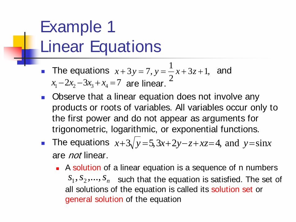
Example 1Linear Equations
The equations andare linear.
Observe that a linear equation does not involve any products or roots of variables. All variables occur only to the first power and do not appear as arguments for trigonometric, logarithmic, or exponential functions. The equations are not linear.
A solution of a linear equation is a sequence of n numbers such that the equation is satisfied. The set of
all solutions of the equation is called its solution set or general solution of the equation
,1321,73 ++==+ zxyyx
732 4321 =+−− xxxx
xyxzzyxyx sin and ,423 ,53 ==+−+=+
nsss ,...,, 21
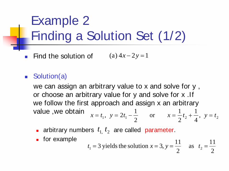
Example 2Finding a Solution Set (1/2)Find the solution of
Solution(a)we can assign an arbitrary value to x and solve for y , or choose an arbitrary value for y and solve for x .If we follow the first approach and assign x an arbitrary value ,we obtain
arbitrary numbers are called parameter.for example
124 )a( =− yx
2211 ,41
21or
212 , tytxtytx =+=−==
2,1 tt
211 as
211,3solution theyields 3 21 ==== tyxt

Example 2Finding a Solution Set (2/2)
Find the solution of
Solution(b)we can assign arbitrary values to any two variables and solve for the third variable.
for example
where s, t are arbitrary values
.574 (b) 321 =+− xxx
txsxtsx ==−+= 321 , ,745

Linear Systems (1/2)A finite set of linear equations in the variablesis called a system of linear equations or a linear system .
A sequence of numbers is called a solution
of the system.
A system has no solution is said to be inconsistent ; if there is at least one solution of the system, it is called consistent.
nxxx ,...,, 21
nsss ,...,, 21mnmnmm
nn
nn
bxaxaxa
bxaxaxabxaxaxa
=+++
=+++=+++
... ... ...
2211
22222121
11212111
MMMM
An arbitrary system of mlinear equations in n unknowns

Linear Systems (2/2)Every system of linear equations has either no solutions, exactly one solution, or infinitely many solutions.
A general system of two linear equations: (Figure1.1.1)
Two lines may be parallel -> no solutionTwo lines may intersect at only one point-> one solutionTwo lines may coincide -> infinitely many solution
zero)both not ,( zero)both not ,(
22222
11111
bacybxabacybxa
=+=+

Augmented Matrices
mnmnmm
nn
nn
bxaxaxa
bxaxaxabxaxaxa
=+++
=+++=+++
... ... ...
2211
22222121
11212111
MMMM
⎥⎥⎥⎥
⎦
⎤
⎢⎢⎢⎢
⎣
⎡
mmnmm
n
n
baaa
baaabaaa
...
... ...
21
222221
111211
MMMM
The location of the +’s, the x’s, and the =‘s can be abbreviated by writing only the rectangular array of numbers.This is called the augmented matrix for the system.Note: must be written in the same order in each equation as the unknowns and the constants must be on the right.
1th column
1th row
Elementary Row OperationsThe basic method for solving a system of linear equations is to replace the given system by a new system that has the same solution set but which is easier to solve.
Since the rows of an augmented matrix correspond to the equations in the associated system. new systems is generally obtained in a series of steps by applying the following three types of operations to eliminate unknowns systematically. These are called elementary row operations.1. Multiply an equation through by an nonzero constant.2. Interchange two equation.3. Add a multiple of one equation to another.

Example 3Using Elementary row Operations(1/4)
0 563 7 172
9 2
=−+−=−
=++
zyxzyzyx
⎯⎯⎯⎯⎯ →⎯ second thetoequation first the
times2- add
0563 134292
=−+=−+=++
zyxzyxzyx
⎯⎯⎯⎯⎯ →⎯ third thetoequation first the
times3- add
⎥⎥⎥
⎦
⎤
⎢⎢⎢
⎣
⎡
−−
056313429211
⎥⎥⎥
⎦
⎤
⎢⎢⎢
⎣
⎡
−−−
0563177209211
⎯⎯⎯ →⎯ third theto rowfirst the times3- add
⎯⎯⎯⎯ →⎯ second theto rowfirst the times2- add
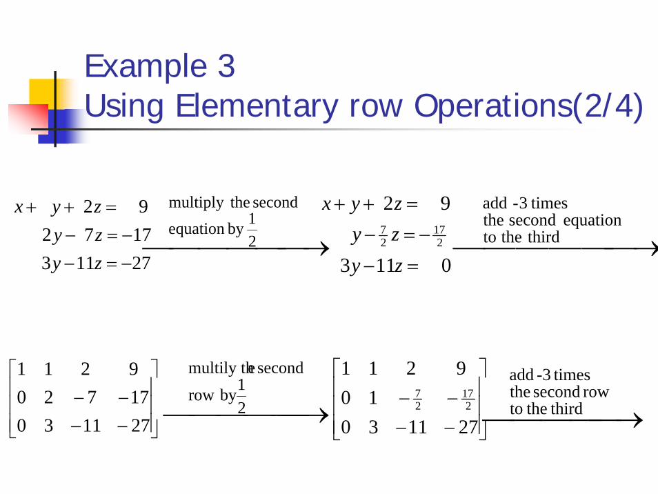
Example 3Using Elementary row Operations(2/4)
0 113
9 2
217
27
=−
−=−
=++
zyzyzyx
⎯⎯⎯⎯⎯ →⎯
21by equation
second themultiply
27113
177 2 9 2
−=−−=−
=++
zyzyzyx
⎥⎥⎥
⎦
⎤
⎢⎢⎢
⎣
⎡
−−−−
271130177209211
⎥⎥⎥
⎦
⎤
⎢⎢⎢
⎣
⎡
−−−−
27113010
9211
217
27
⎯⎯⎯⎯⎯ →⎯ third thetoequation second the times3- add
⎯⎯⎯⎯ →⎯ third theto row second the
times3- add
⎯⎯⎯⎯⎯ →⎯
21by row
second emultily th
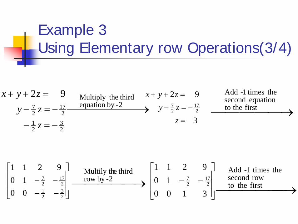
Example 3Using Elementary row Operations(3/4)
3
9 2
217
27
=
−=−
=++
zzyzyx
⎯⎯⎯⎯⎯ →⎯ 2-by equation thirdtheMultiply
23
21
217
27
9 2
−=−
−=−
=++
zzyzyx
⎥⎥⎥
⎦
⎤
⎢⎢⎢
⎣
⎡
−−−−
23
21
217
27
0010
9211
⎥⎥⎥
⎦
⎤
⎢⎢⎢
⎣
⎡−−3100
109211
217
27
⎯⎯⎯⎯⎯ →⎯ first theto row second
the times1- Add
⎯⎯⎯⎯ →⎯ 2-by row thirdeMultily th
⎯⎯⎯⎯ →⎯ first thetoequation second
the times1- Add

Example 3Using Elementary row Operations(4/4)
3 2
1
===
zy
x
⎯⎯⎯⎯⎯⎯ →⎯ second thetoequation thirdthe
times andfirst thetoequation thirdthe
times- Add
27
211
3
217
27
235
211
=
−=−
=+
zzyzx
⎥⎥⎥
⎦
⎤
⎢⎢⎢
⎣
⎡−−3100
1001
217
27
235
211
⎥⎥⎥
⎦
⎤
⎢⎢⎢
⎣
⎡
310020101001
⎯⎯⎯⎯⎯ →⎯ second thetorow third thetimes
andfirst theto row thirdthe times- Add
27
211
The solution x=1,y=2,z=3 is now evident.
1.2 Gaussian Elimination

Echelon FormsThis matrix which have following properties is in reduced row-echelon form (Example 1, 2).
1. If a row does not consist entirely of zeros, then the firstnonzero number in the row is a 1. We call this a leader 1.
2. If there are any rows that consist entirely of zeros, then they are grouped together at the bottom of the matrix.
3. In any two successive rows that do not consist entirely of zeros, the leader 1 in the lower row occurs farther to the right than the leader 1 in the higher row.
4. Each column that contains a leader 1 has zeros everywhere else.A matrix that has the first three properties is said to be in row-echelon form (Example 1, 2).A matrix in reduced row-echelon form is of necessity in row-echelon form, but not conversely.

Example 1Row-Echelon & Reduced Row-Echelon form
reduced row-echelon form:
⎥⎦
⎤⎢⎣
⎡
⎥⎥⎥⎥
⎦
⎤
⎢⎢⎢⎢
⎣
⎡ −
⎥⎥⎥
⎦
⎤
⎢⎢⎢
⎣
⎡
⎥⎥⎥
⎦
⎤
⎢⎢⎢
⎣
⎡
−0000
,
00000000003100010210
,100010001
,1100
70104001
row-echelon form:
⎥⎥⎥
⎦
⎤
⎢⎢⎢
⎣
⎡−
⎥⎥⎥
⎦
⎤
⎢⎢⎢
⎣
⎡
⎥⎥⎥
⎦
⎤
⎢⎢⎢
⎣
⎡ −
100000110006210
,000010011
,510026107341

Example 2More on Row-Echelon and Reduced Row-Echelon form
All matrices of the following types are in row-echelon form ( any real numbers substituted for the *’s. ) :
⎥⎥⎥⎥⎥⎥
⎦
⎤
⎢⎢⎢⎢⎢⎢
⎣
⎡
⎥⎥⎥⎥
⎦
⎤
⎢⎢⎢⎢
⎣
⎡
⎥⎥⎥⎥
⎦
⎤
⎢⎢⎢⎢
⎣
⎡
⎥⎥⎥⎥
⎦
⎤
⎢⎢⎢⎢
⎣
⎡
*100000000*0**100000*0**010000*0**001000*0**000*10
,
00000000**10**01
,
0000*100*010*001
,
1000010000100001
⎥⎥⎥⎥⎥⎥
⎦
⎤
⎢⎢⎢⎢⎢⎢
⎣
⎡
⎥⎥⎥⎥
⎦
⎤
⎢⎢⎢⎢
⎣
⎡
⎥⎥⎥⎥
⎦
⎤
⎢⎢⎢⎢
⎣
⎡
⎥⎥⎥⎥
⎦
⎤
⎢⎢⎢⎢
⎣
⎡
*100000000****100000*****10000******1000********10
,
00000000**10***1
,
0000*100**10***1
,
1000*100**10***1
All matrices of the following types are in reduced row-echelon form ( any real numbers substituted for the *’s. ) :

Example 3Solutions of Four Linear Systems (a)
⎥⎥⎥
⎦
⎤
⎢⎢⎢
⎣
⎡−41002010
5001 (a)
4 2-
5
===
zy
x
Solution (a)
the corresponding system of equations is :
Suppose that the augmented matrix for a system of linear equations have been reduced by row operations to the given reduced row-echelon form. Solve the system.

Example 3Solutions of Four Linear Systems (b1)
⎥⎥⎥
⎦
⎤
⎢⎢⎢
⎣
⎡ −
231006201014001
(b)
Solution (b)
1. The corresponding system of equations is :
2 3 6 2 1- 4
43
42
41
=+=+=+
xxxxxx
leading variables
free variables

Example 3Solutions of Four Linear Systems (b2)
43
42
41
3-2 2- 6 4 - 1-
xxxxxx
===
txtxtxtx
,32 ,26 ,41
4
3
2
1
=−=−=−−=3. There are infinitely many
solutions, and the general solution is given by the formulas
2. We see that the free variable can be assigned an arbitrary value, say t, which then determines values of the leading variables.
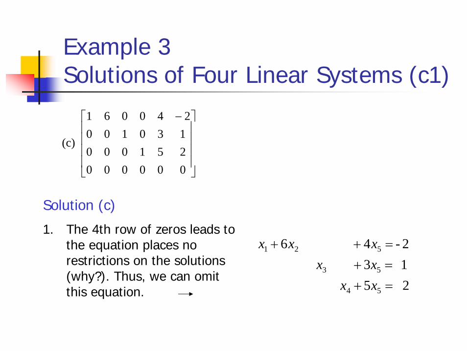
Example 3Solutions of Four Linear Systems (c1)
⎥⎥⎥⎥
⎦
⎤
⎢⎢⎢⎢
⎣
⎡ −
000000251000130100240061
(c)
2 5 1 3
2- 4 6
54
53
521
=+=+=++
xxxxxxx
Solution (c)
1. The 4th row of zeros leads to the equation places no restrictions on the solutions (why?). Thus, we can omit this equation.
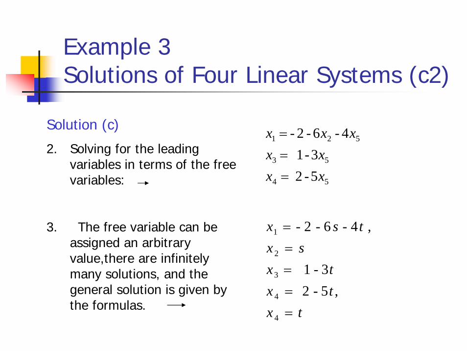
Example 3Solutions of Four Linear Systems (c2)
Solution (c)
2. Solving for the leading variables in terms of the free variables:
3. The free variable can be assigned an arbitrary value,there are infinitely many solutions, and the general solution is given by the formulas.
54
53
521
5-2 3- 1
4-6- 2-
xxxx
xxx
===
txtxtx
sxtsx
=====
4
4
3
2
1
,5-2 3- 1
, 4-6- 2-

Example 3Solutions of Four Linear Systems (d)
⎥⎥⎥
⎦
⎤
⎢⎢⎢
⎣
⎡
100002100001
(d)
Solution (d):
the last equation in the corresponding system of equation is
Since this equation cannot be satisfied, there is no solution to the system.
1000 321 =++ xxx

Elimination Methods (1/7)We shall give a step-by-step eliminationprocedure that can be used to reduce any matrix to reduced row-echelon form.
⎥⎥⎥
⎦
⎤
⎢⎢⎢
⎣
⎡
−−−−−
1565422812610421270200
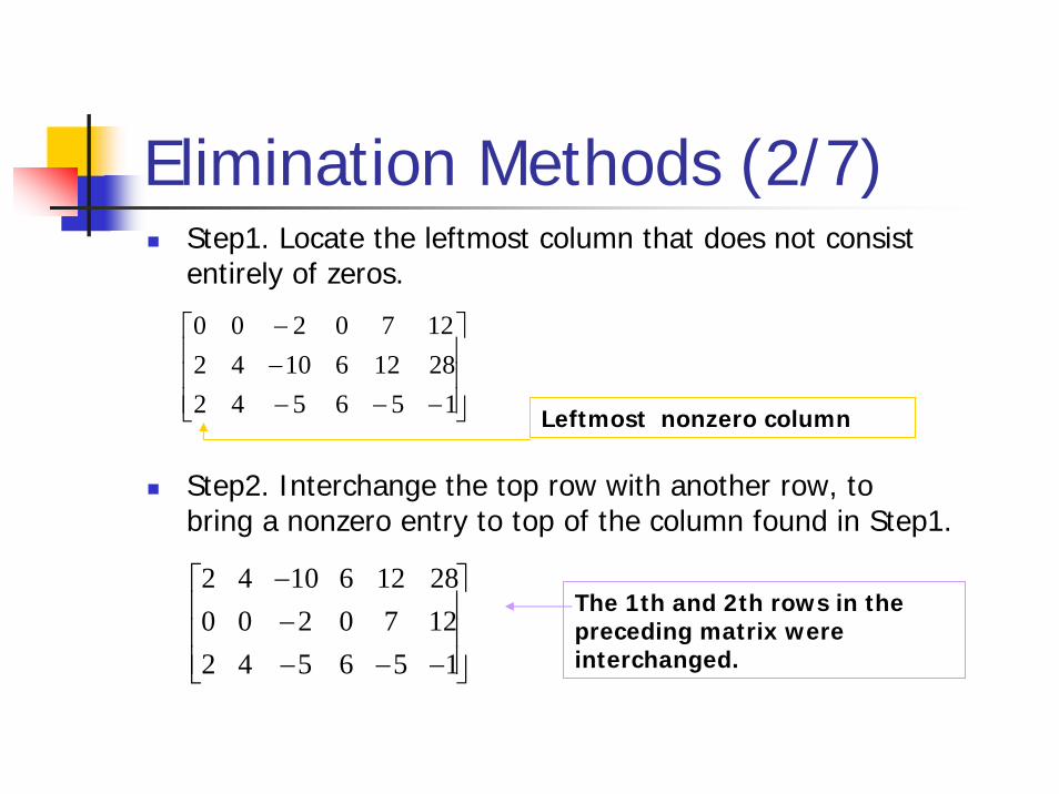
Elimination Methods (2/7)Step1. Locate the leftmost column that does not consist entirely of zeros.
Step2. Interchange the top row with another row, to bring a nonzero entry to top of the column found in Step1.
⎥⎥⎥
⎦
⎤
⎢⎢⎢
⎣
⎡
−−−−−
1565422812610421270200
Leftmost nonzero column
⎥⎥⎥
⎦
⎤
⎢⎢⎢
⎣
⎡
−−−−−
1565421270200281261042
The 1th and 2th rows in the preceding matrix were interchanged.
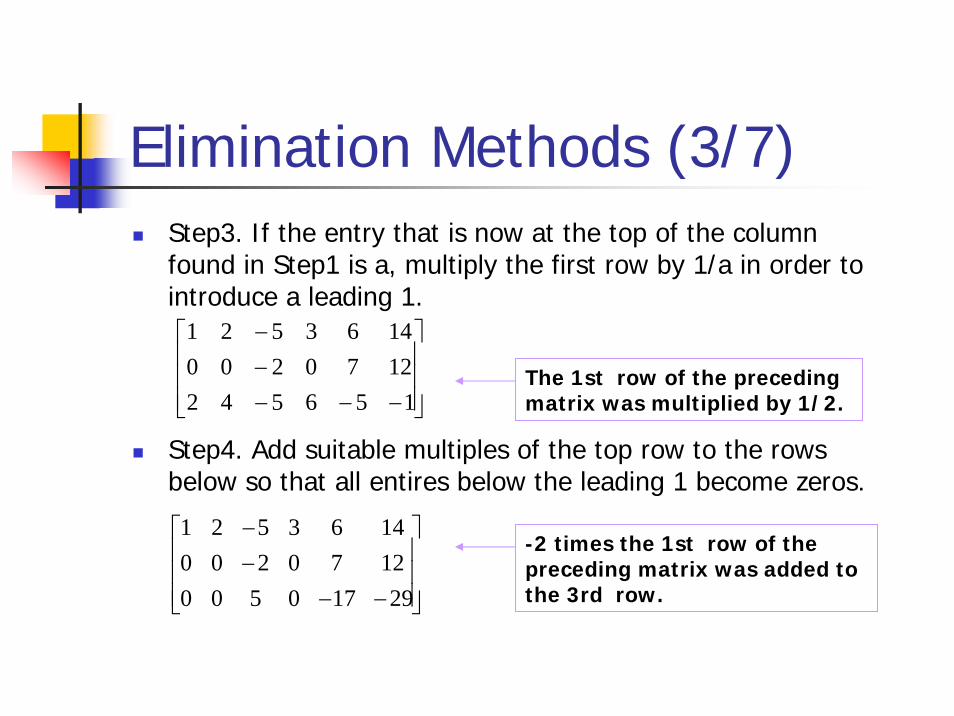
Elimination Methods (3/7)Step3. If the entry that is now at the top of the column found in Step1 is a, multiply the first row by 1/a in order to introduce a leading 1.
Step4. Add suitable multiples of the top row to the rows below so that all entires below the leading 1 become zeros.
⎥⎥⎥
⎦
⎤
⎢⎢⎢
⎣
⎡
−−−−−
15654212702001463521
The 1st row of the preceding matrix was multiplied by 1/2.
⎥⎥⎥
⎦
⎤
⎢⎢⎢
⎣
⎡
−−−−
2917050012702001463521
-2 times the 1st row of the preceding matrix was added to the 3rd row.

Elimination Methods (4/7)Step5. Now cover the top row in the matrix and begin again with Step1 applied to the submatrix that remains. Continue in this way until the entire matrix is in row-echelon form.
⎥⎥⎥
⎦
⎤
⎢⎢⎢
⎣
⎡
−−−−−
2917050012702001463521
The 1st row in the submatrixwas multiplied by -1/2 to introduce a leading 1.⎥
⎥⎥
⎦
⎤
⎢⎢⎢
⎣
⎡
−−−−
−
2917050060100
1463521
27
Leftmost nonzero column in the submatrix
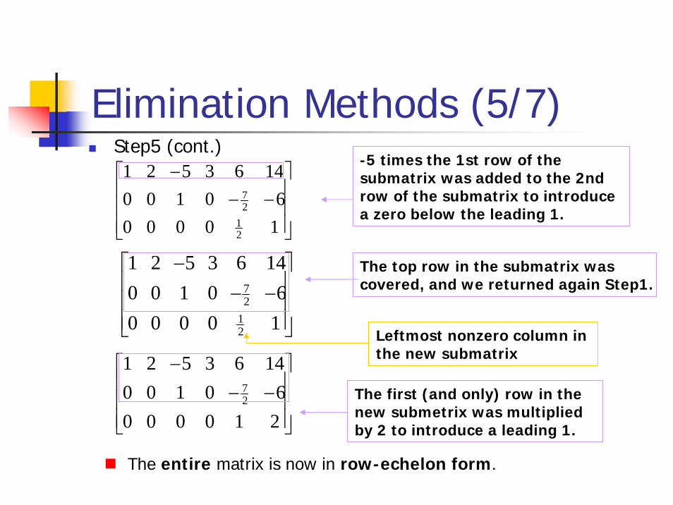
Elimination Methods (5/7)Step5 (cont.)
⎥⎥⎥
⎦
⎤
⎢⎢⎢
⎣
⎡−−
−
21000060100
1463521
27
-5 times the 1st row of the submatrix was added to the 2nd row of the submatrix to introduce a zero below the leading 1.
⎥⎥⎥
⎦
⎤
⎢⎢⎢
⎣
⎡−−
−
1000060100
1463521
21
27
⎥⎥⎥
⎦
⎤
⎢⎢⎢
⎣
⎡−−
−
1000060100
1463521
21
27
The top row in the submatrix was covered, and we returned again Step1.
The first (and only) row in the new submetrix was multiplied by 2 to introduce a leading 1.
Leftmost nonzero column in the new submatrix
The entire matrix is now in row-echelon form.

Elimination Methods (6/7)Step6. Beginning with las nonzero row and working upward, add suitable multiples of each row to the rows above to introduce zeros above the leading 1’s.
⎥⎥⎥
⎦
⎤
⎢⎢⎢
⎣
⎡
210000100100703021
7/2 times the 3rd row of the preceding matrix was added to the 2nd row.
⎥⎥⎥
⎦
⎤
⎢⎢⎢
⎣
⎡ −
2100001001001463521
⎥⎥⎥
⎦
⎤
⎢⎢⎢
⎣
⎡ −
210000100100203521
-6 times the 3rd row was added to the 1st row.
The last matrix is in reduced row-echelon form.
5 times the 2nd row was added to the 1st row.

Elimination Methods (7/7)Step1~Step5: the above procedure produces a row-echelon form and is called Gaussian elimination.Step1~Step6: the above procedure produces a reduced row-echelon form and is called Gaussian-Jordan elimination.Every matrix has a unique reduced row-echelon form but a row-echelon form of a given matrix is not unique.

Example 4Gauss-Jordan Elimination(1/4)
Solve by Gauss-Jordan Elimination
Solution:The augmented matrix for the system is
6 18 48 625 15 105 13 42 5620 x2 23
65421
643
654321
5321
=−+++=++−=−+−−+
=+−+
xxxxxxxxxxxxxx
xxx
⎥⎥⎥⎥
⎦
⎤
⎢⎢⎢⎢
⎣
⎡
618480625150105001-3-42-5-62
00202-31

Example 4Gauss-Jordan Elimination(2/4)
Adding -2 times the 1st row to the 2nd and 4th rows gives
Multiplying the 2nd row by -1 and then adding -5 times the new 2nd row to the 3rd row and -4 times the new 2nd row to the 4th row gives
⎥⎥⎥⎥
⎦
⎤
⎢⎢⎢⎢
⎣
⎡
2600000000000013-0210000202-31
⎥⎥⎥⎥
⎦
⎤
⎢⎢⎢⎢
⎣
⎡
618084005150105001-3-02-1-00
00202-31
Example 4Gauss-Jordan Elimination(3/4)
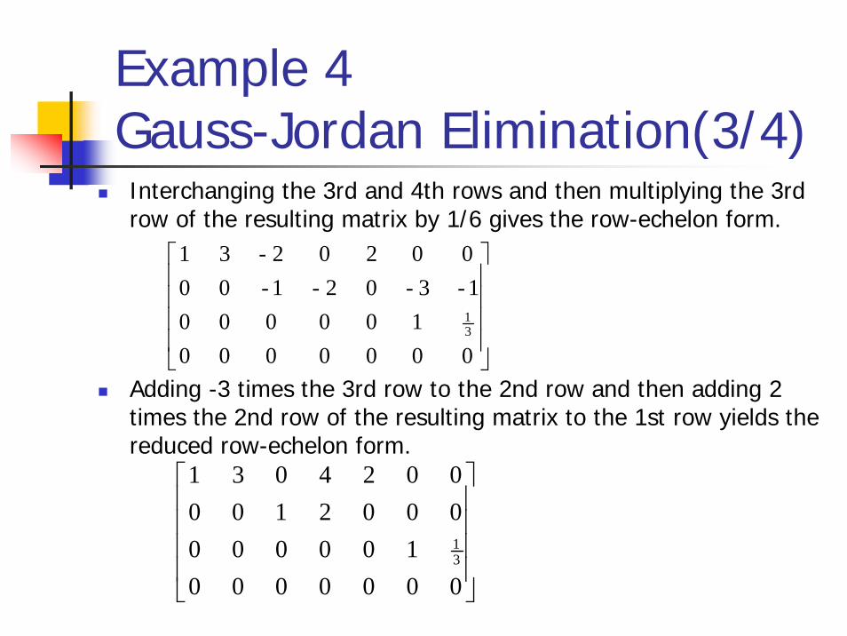
Interchanging the 3rd and 4th rows and then multiplying the 3rd row of the resulting matrix by 1/6 gives the row-echelon form.
Adding -3 times the 3rd row to the 2nd row and then adding 2 times the 2nd row of the resulting matrix to the 1st row yields the reduced row-echelon form.
⎥⎥⎥⎥
⎦
⎤
⎢⎢⎢⎢
⎣
⎡
0000000100000
00021000024031
31
⎥⎥⎥⎥
⎦
⎤
⎢⎢⎢⎢
⎣
⎡
0000000100000
1-3-02-1-0000202-31
31

Example 4Gauss-Jordan Elimination(4/4)
The corresponding system of equations is
SolutionThe augmented matrix for the system is
We assign the free variables, and the general solution is given by the formulas:
31
6
43
5421
0 2 0 x24 3
=
=+=+++
xxxxxx
31
6
43
5421
2
x243
=
−=−−−=
xxx
xxx
31
654321 , , ,2 , ,243 ===−==−−−= xtxsxsxrxtsrx

Back-SubstitutionIt is sometimes preferable to solve a system of linear equations by using Gaussian elimination to bring the augmented matrix into row-echelon form without continuing all the way to the reduced row-echelon form.When this is done, the corresponding system of equations can be solved by solved by a technique called back-substitution.Example 5
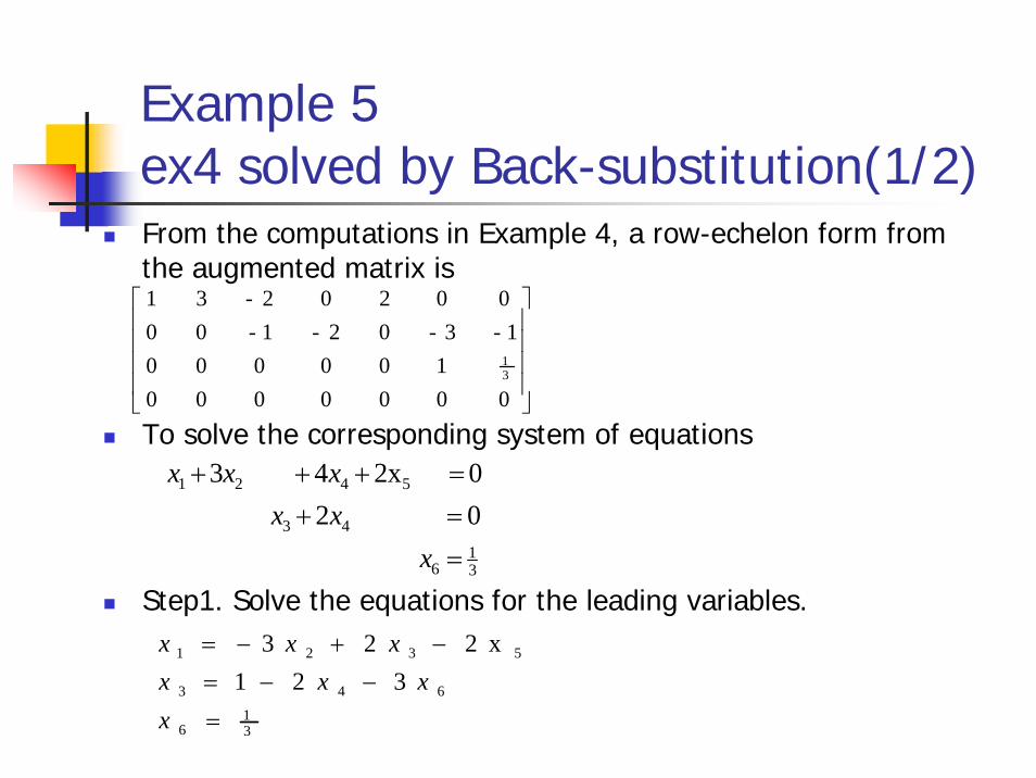
Example 5 ex4 solved by Back-substitution(1/2)From the computations in Example 4, a row-echelon form from the augmented matrix is
To solve the corresponding system of equations
Step1. Solve the equations for the leading variables.
⎥⎥⎥⎥
⎦
⎤
⎢⎢⎢⎢
⎣
⎡
0000000100000
1-3-02-1-0000202-31
31
31
6
43
5421
0 2 0 x24 3
=
=+=+++
xxxxxx
31
6
643
5321
321
x223
=
−−=−+−=
xxxx
xxx

Example5ex4 solved by Back-substitution(2/2)Step2. Beginning with the bottom equation and working upward, successively substitute each equation into all the equations above it.
Substituting x6=1/3 into the 2nd equation
Substituting x3=-2 x4 into the 1st equation
Step3. Assign free variables, the general solution is given by the formulas.
31
6
43
5321
2
x223
=
−=−+−=
xxx
xxx
31
6
43
5321
2
x223
=
−=−+−=
xxx
xxx
31
654321 , , ,2 , ,243 ===−==−−−= xtxsxsxrxtsrx
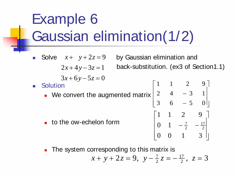
Example 6Gaussian elimination(1/2)
Solve by Gaussian elimination andback-substitution. (ex3 of Section1.1)
SolutionWe convert the augmented matrix
to the ow-echelon form
The system corresponding to this matrix is
0563 134292
=−+=−+=++
zyxzyxzyx
⎥⎥⎥
⎦
⎤
⎢⎢⎢
⎣
⎡
−−
056313429211
⎥⎥⎥
⎦
⎤
⎢⎢⎢
⎣
⎡−−
310010
9211 2
1727
3 , ,92 17722 =−=−=++ zzyzyx

Example 6Gaussian elimination(2/2)
SolutionSolving for the leading variables
Substituting the bottom equation into those above
Substituting the 2nd equation into the top
3 ,2
,3
==
−=
zy
yx
3 ,
,29
27
217
=
+−=−−=
zzyzyx
3 ,2 ,1 === zyx

Homogeneous Linear Systems(1/2)A system of linear equations is said to be homogeneous if the constant terms are all zero; that is , the system has the form :
Every homogeneous system of linear equation is consistent, since all such system haveas a solution. This solution is called the trivial solution; if there are another solutions, they are called nontrivial solutions. There are only two possibilities for its solutions:
The system has only the trivial solution.The system has infinitely many solutions in addition to the trivial solution.
0... 0 ...0 ...
2211
2222121
1212111
=+++
=+++=+++
nmnmm
nn
nn
xaxaxa
xaxaxaxaxaxa
MMMM
0,...,0,0 21 === nxxx

Homogeneous Linear Systems(2/2)
In a special case of a homogeneous linear system of two linear equations in two unknowns: (fig1.2.1)
zero)both not ,( 0zero)both not ,( 0
2222
1111
baybxabaybxa
=+=+

Example 7Gauss-Jordan Elimination(1/3)
0 0 2 0 32 0 2 2
543
5321
54321
5321
=++=−−+=+−+−−=+−+
xxxxxxxxxxxxxxxx
⎥⎥⎥⎥
⎦
⎤
⎢⎢⎢⎢
⎣
⎡
−−−−−
−
001000010211013211010122
⎥⎥⎥⎥
⎦
⎤
⎢⎢⎢⎢
⎣
⎡
000000001000010100010011
Solve the following homogeneous system of linear equations by using Gauss-Jordan elimination.
Solution The augmented matrix
Reducing this matrix to reduced row-echelon form

Example 7Gauss-Jordan Elimination(2/3)
0 0 0
4
53
521
==+=++
xxxxxx
0
4
53
521
=−=
−−=
xxx
xxx
Solution (cont)The corresponding system of equation
Solving for the leading variables is
Thus the general solution is
Note: the trivial solution is obtained when s=t=0.
txxtxsxtsx ==−==−−= 54321 ,0 , , ,

Example7Gauss-Jordan Elimination(3/3)
(1) 0()
0()
0()
2
1
=+
=+
=+
∑
∑∑
r
k
k
x
x
x
MO
L
L
(2) ()
()
()
2
1
∑
∑∑
−=
−=
−=
r
k
k
x
x
x
M
Two important points:Non of the three row operations alters the final column of zeros, so the system of equations corresponding to the reduced row-echelon form of the augmented matrix must also be a homogeneous system.If the given homogeneous system has m equations in n unknowns with m<n, and there are r nonzero rows in reduced row-echelon form of the augmented matrix, we will have r<n. It will have the form:
Theorem 1.2.1
A homogeneous system of linear equations with more unknowns than equations has infinitely many solutions.
Note: theorem 1.2.1 applies only to homogeneous systemExample 7 (3/3)
Computer Solution of Linear System
Most computer algorithms for solving large linear systems are based on Gaussian elimination or Gauss-Jordan elimination.Issues
Reducing roundoff errorsMinimizing the use of computer memory spaceSolving the system with maximum speed

Reference
http://vision.ee.ccu.edu.tw/modules/tinyd2/content/93_LA/Chapter1(1.1~1.3).ppt