Linear algebra basics
48
Appendix A Linear algebra basics A.1 Linear spaces Linear spaces consist of elements called vectors. Vectors are abstract mathematical objects, but, as the name suggests, they can be visualized as geometric vectors. Like regular numbers, vectors can be added together and subtracted from each other to form new vectors; they can also be multiplied by numbers. However, vectors cannot be multiplied or divided by one another as numbers can. One important peculiarity of the linear algebra used in quantum mechanics is the so-called Dirac notation for vectors. To denote vectors, instead of writing, for example, ~ a, we write |ai. We shall see later how convenient this notation turns out to be. Definition A.1. A linear (vector) space V over a field 1 F is a set in which the following operations are defined: 1. Addition: for any two vectors |ai , |bi∈ V, there exists a unique vector in V called their sum, denoted by |ai + |bi. 2. Multiplication by a number (“scalar”): For any vector |ai∈ V and any number λ ∈ F, there exists a unique vector in V called their product, denoted by λ |ai≡ |ai λ . These operations obey the following axioms. 1. Commutativity of addition: |ai + |bi = |bi + |ai. 2. Associativity of addition: (|ai + |bi)+ |ci = |ai +(|bi + |ci). 3. Existence of zero: there exists an element of V called |zeroi such that, for any A. I. Lvovsky, Quantum Physics, Undergraduate Lecture Notes in Physics, https://doi.org/10.1007/978-3-662-56584-1 255 1 Field is a term from algebra which means a complete set of numbers. The sets of rational numbers Q, real numbers R, and complex numbers C are examples of fields. Quantum mechanics usually deals with vector spaces over the field of complex numbers. A solutions manual for this appendix is available for download at https://www.springer.com/gp/book/9783662565827 As an alternative notation for |zero〉, we some times use “0” but not “|0〉”. 2 vector |ai, |ai + |zeroi |i = a . 2 © Springer-Verlag GmbH Germany, part of Springer Nature 2018
-
Upload
khangminh22 -
Category
Documents
-
view
1 -
download
0
Transcript of Linear algebra basics
Appendix ALinear algebra basics
A.1 Linear spaces
Linear spaces consist of elements called vectors. Vectors are abstract mathematicalobjects, but, as the name suggests, they can be visualized as geometric vectors. Likeregular numbers, vectors can be added together and subtracted from each other toform new vectors; they can also be multiplied by numbers. However, vectors cannotbe multiplied or divided by one another as numbers can.
One important peculiarity of the linear algebra used in quantum mechanics isthe so-called Dirac notation for vectors. To denote vectors, instead of writing, forexample, ~a, we write |a〉. We shall see later how convenient this notation turns outto be.
Definition A.1. A linear (vector) space V over a field1 F is a set in which thefollowing operations are defined:
1. Addition: for any two vectors |a〉 , |b〉 ∈ V, there exists a unique vector in Vcalled their sum, denoted by |a〉+ |b〉.
2. Multiplication by a number (“scalar”): For any vector |a〉 ∈ V and any numberλ ∈ F, there exists a unique vector in V called their product, denoted by λ |a〉 ≡|a〉λ .
These operations obey the following axioms.
1. Commutativity of addition: |a〉+ |b〉= |b〉+ |a〉.2. Associativity of addition: (|a〉+ |b〉)+ |c〉= |a〉+(|b〉+ |c〉).3. Existence of zero: there exists an element of V called |zero〉 such that, for any
A. I. Lvovsky, Quantum Physics, Undergraduate Lecture Notes inPhysics, https://doi.org/10.1007/978-3-662-56584-1
255
1 Field is a term from algebra which means a complete set of numbers. The sets of rational numbersQ, real numbers R, and complex numbers C are examples of fields. Quantum mechanics usuallydeals with vector spaces over the field of complex numbers.
A solutions manual for this appendix is available for download at
https://www.springer.com/gp/book/9783662565827
As an alternative notation for |zero〉, we some times use “0” but not “|0〉”.2
vector |a〉, |a〉+ |zero〉 | 〉= a .2
© Springer-Verlag GmbH Germany, part of Springer Nature 2018
256 A. I. Lvovsky. Quantum Physics
4. Existence of the opposite element: For any vector |a〉 there exists another vector,denoted by −|a〉, such that |a〉+(−|a〉) = |zero〉.
5. Distributivity of vector sums: λ (|a〉+ |b〉) = λ |a〉+λ |b〉.6. Distributivity of scalar sums: (λ +µ) |a〉= λ |a〉+µ |a〉.7. Associativity of scalar multiplication: λ (µ |a〉) = (λ µ) |a〉.8. Scalar multiplication identity: For any vector |a〉 and number 1∈ F, 1 · |a〉= |a〉.
Definition A.2. Subtraction of vectors in a linear space is defined as follows:
|a〉− |b〉 ≡ |a〉+(−|b〉).
Exercise A.1. Which of the following are linear spaces (over the field of complexnumbers, unless otherwise indicated)?
a) R over R? R over C? C over R? C over C?b) Polynomial functions? Polynomial functions of degree ≤ n? > n?c) All functions such that f (1) = 0? f (1) = 1?d) All periodic functions of period T ?e) N-dimensional geometric vectors over R?
Exercise A.2. Prove the following:
a) there is only one zero in a linear space;b) if |a〉+ |x〉= |a〉 for some |a〉 ∈ V, then |x〉= |zero〉;c) for any vector |a〉 and for number 0 ∈ F, 0 |a〉= |zero〉;d) −|a〉= (−1) |a〉;e) −|zero〉= |zero〉;f) for any |a〉, −|a〉 is unique;g) −(−|a〉) = |a〉;h) |a〉= |b〉 if and only if |a〉− |b〉= 0.
Hint: Most of these propositions can be proved by adding the same number to thetwo sides of an equality.
A.2 Basis and dimension
Definition A.3. A set of vectors |vi〉 is said to be linearly independent if no nontri-vial2 linear combination λ1 |v1〉+ . . .+λN |vN〉 equals |zero〉.Exercise A.3. Show that a set of vectors {|vi〉} is not linearly independent if andonly if one of the |vi〉 can be represented as a linear combination of others.
Exercise A.4. For linear spaces of geometric vectors, show the following:
a) For the space of vectors in a plane (denoted R ), any two vectors are linearly in-dependent if and only if they are not parallel. Any set of three vectors is linearlydependent.
That is, in which at least one of the coefficients is nonzero.3
3
A.2 Basis and dimension 257
b) For the space of vectors in a three-dimensional space (denoted R ), any threenon-coplanar vectors form a linearly independent set.
Hint: Recall that a geometric vector can be defined by its x, y and z components.
Definition A.4. A subset {|vi〉} of a vector space V is said to span V (or to be aspanning set for V) if any vector in V can be expressed as a linear combination ofthe |vi〉.
Exercise A.5. For the linear space of geometric vectors in a plane, show that anyset of at least two vectors, of which at least two are non-parallel, forms a spanningset.
Definition A.5. A basis of V is any linearly independent spanning set. A decompo-sition of a vector relative to a basis is its expression as a linear combination of thebasis elements.
The basis is a smallest subset of a linear space such that all other vectors canbe expressed as a linear combination of the basis elements. The term “basis” maysuggest that each linear space has only one basis — just as a building can have onlyone foundation. Actually, as we shall see, in any nontrivial linear space, there areinfinitely many bases.
Definition A.6. The number of elements in a basis is called the dimension of V.Notation: dimV.
Exercise A.6.∗ Prove that in a finite-dimensional space, all bases have the samenumber of elements.
Exercise A.7. Using the result of Ex. A.6, show that, in a finite-dimensional space,
a) any linearly independent set of N = dimV vectors forms a basis;b) any spanning set of N = dimV vectors forms a basis.
Exercise A.8. Show that, for any element of V, there exists only one decompositioninto basis vectors.
Definition A.7. For a decomposition of the vector |a〉 into basis {|vi〉}, viz.,
|a〉= ∑i
ai |vi〉 , (A.1)
we may use the notation
|a〉 '
a1...
aN
. (A.2)
This is called the matrix form of a vector, in contrast to the Dirac form (A.1). Thescalars ai are called the coefficients or amplitudes of the decomposition3.
We use the symbol ' instead of = when expressing vectors and operators in matrix form, e.g.,in Eq. (A.2). This is to emphasize the difference: the left-hand side, a vector, is an abstract object
4
4
258 A. I. Lvovsky. Quantum Physics
Exercise A.9. Let |a〉 be one of the elements, |vk〉, of the basis {|vi〉}. Find thematrix form of the decomposition of |a〉 into this basis.
Exercise A.10. Consider the linear space of two-dimensional geometric vectors.Such vectors are usually defined by two numbers (x,y), which correspond to their xand y components, respectively. Does this notation correspond to a decompositioninto any basis? If so, which one?
Exercise A.11. Show the following:
a) For the linear space of geometric vectors in a plane, any two non-parallel vectorsform a basis.
b) For the linear space of geometric vectors in a three-dimensional space, any threenon-coplanar vectors form a basis.
Exercise A.12. Consider the linear space of two-dimensional geometric vec-tors. The vectors ~a,~b,~c, ~d are oriented with respect to the x axis at angles0, 45◦, 90◦, 180◦ and have lengths 2, 1, 3, 1, respectively. Do the pairs {~a,~c}, {~b, ~d},{~a, ~d} form bases? Find the decompositions of the vector~b in each of these bases.Express them in the matrix form.
Definition A.8. A subset of a linear space V that is a linear space on its own iscalled a subspace of V.
Exercise A.13. In an arbitrary basis {|vi〉} in the linear space V, a subset of elementsis taken. Show that a set of vectors that are spanned by this subset is a subspace ofV.
For example, in the space of three-dimensional geometric vectors, any set ofvectors within a particular plane or any set of vectors collinear to a given straightline form a subspace.
A.3 Inner Product
Although vectors cannot be multiplied together in the same way that numbers can,one can define a multiplication operation that maps any pair of vectors onto a num-ber. This operation generalizes the scalar product that is familiar from geometry.
Definition A.9. For any two vectors |a〉, |b〉 ∈ V we define an inner (scalar) pro-duct — a number 〈a| b〉 ∈ C such that:
1. For any three vectors |a〉 , |b〉 , |c〉 , 〈a|(|b〉+ |c〉) = 〈a| b〉+ 〈a| c〉.2. For any two vectors |a〉 , |b〉 and number λ , 〈a|(λ |b〉) = λ 〈a| b〉.
and is basis-independent, while the right-hand side is a set of numbers and depends on the choiceof basis {|vi〉}. However, in the literature, the equality sign is generally used for simplicity.
The inner product of two vectors is sometimes called the overlap in the context of quantumphysics.
5
5
A.4 Orthonormal Basis 259
3. For any two vectors |a〉 , |b〉 , 〈a| b〉= 〈b| a〉∗.4. For any |a〉 , 〈a| a〉 is a nonnegative real number, and 〈a| a〉 = 0 if and only if|a〉= 0.
Exercise A.14. In geometry, the scalar product of two vectors ~a = (xa,ya) and~b =
(xb,yb) (where all components are real) is defined as ~a ·~b = xaxb + yayb. Show thatthis definition has all the properties listed above.
Exercise A.15. Suppose a vector |x〉 is written as a linear combination of somevectors |ai〉: |x〉= ∑i λi |ai〉. For any other vector |b〉, show that 〈b| x〉= ∑i λi 〈b| ai〉and 〈x| b〉= ∑i λ ∗i 〈ai| b〉.
Exercise A.16. For any vector |a〉, show that 〈zero| a〉= 〈a| zero〉= 0.
Definition A.10. |a〉 and |b〉 are said to be orthogonal if 〈a| b〉= 0.
Exercise A.17. Prove that a set of nonzero mutually orthogonal vectors is linearlyindependent.
Definition A.11. ‖|a〉‖=√〈a| a〉 is called the norm (length) of a vector. Vectors of
norm 1 are said to be normalized. For a given vector |a〉, the quantity N = 1/‖|a〉‖(such that the vector N |a〉 is normalized) is called the normalization factor.
Exercise A.18. Show that multiplying a vector by a phase factor eiφ , where φ is areal number, does not change its norm.
Definition A.12. A linear space in which an inner product is defined is called aHilbert space.
A.4 Orthonormal Basis
Definition A.13. An orthonormal basis {|vi〉} is a basis whose elements are mutu-ally orthogonal and have norm 1, i.e.,⟨
vi∣∣ v j⟩= δi j, (A.3)
where δi j is the Kronecker symbol.
Exercise A.19. Show that any orthonormal set of N (where N = dimV) vectorsforms a basis.
Exercise A.20. Show that, if
a1...
aN
and
b1...
bN
are the decompositions of vectors
|a〉 and |b〉 in an orthonormal basis, their inner product can be written in the form
〈a| b〉= a∗1b1 + . . .+a∗NbN . (A.4)
260 A. I. Lvovsky. Quantum Physics
Equation (A.4) can be expressed in matrix form using the “row-times-column”rule:
〈a| b〉=(
a∗1 . . . a∗N) b1
...bN
. (A.5)
One context where we can use the above equations for calculating the inner pro-duct is ordinary spatial geometry. As we found in Ex. A.10, the coordinates of geo-metric vectors correspond to their decomposition into orthogonal basis {i, j}, so notsurprisingly, their scalar products are given by Eq. (A.4).
Suppose we calculate the inner product of the same pair of vectors usingEq. (A.5) in two different bases. Then the right-hand side of that equation willcontain different numbers, so it may seem that the inner product will also dependon the basis chosen. This is not the case, however: according to Defn. A.9, the innerproduct is defined for a pair of vectors, and is basis-independent.
Exercise A.21. Show that the amplitudes of the decomposition
a1...
aN
of a vector
|a〉 into an orthonormal basis can be found as follows:
ai = 〈vi| a〉 . (A.6)
In other words [see Eq. (A.1)],
|a〉= ∑i〈vi| a〉 |vi〉 . (A.7)
Exercise A.22. Consider two vectors in a two-dimensional Hilbert space, |ψ〉 =4 |v1〉+5 |v2〉 and |φ〉=−2 |v1〉+3i |v2〉, where {|v1〉 , |v2〉} is an orthonormal basis.
a) Show that the set {|w1〉= (|v1〉+ i |v2〉)/√
2, |w2〉= (|v1〉− i |v2〉)/√
2} is alsoan orthonormal basis.
b) Find the matrices of vectors |ψ〉 and |φ〉 in both bases.c) Calculate the inner product of these vectors in both bases using Eq. (A.5). Show
that they are the same.
Exercise A.23. Show that, if |a〉 is a normalized vector and {ai = 〈vi| a〉} is itsdecomposition in an orthonormal basis {|vi〉}, then
∑i|ai|2 = 1. (A.8)
Exercise A.24. Suppose {|wi〉} is some basis in V. It can be used to find an ort-honormal basis {|vi〉} by applying the following equation in sequence to each basiselement:
|vk+1〉= N
[|wk+1〉−
k
∑i=1〈vi| wk+1〉 |vi〉
], (A.9)

A.5 Adjoint Space 261
where N is the normalization factor. This is called the Gram-Schmidt procedure.
Exercise A.25.∗ For a normalized vector |ψ〉 in an N-dimensional Hilbert space, andany natural number m ≤ N, show that it is possible to find a basis {|vi〉} such that|ψ〉= 1/
√m∑
mi=1 |vi〉.
Exercise A.26.∗ Prove the Cauchy-Schwarz inequality for any two vectors |a〉 and|b〉:
| 〈a| b〉 | ≤ ‖|a〉‖×‖|b〉‖. (A.10)
Show that the inequality is saturated (i.e., becomes an equality) if and only if thevectors |a〉 and |b〉 are collinear (i.e., |a〉= λ |b〉).Hint: Use the fact that ‖|a〉−λ |b〉‖2 ≥ 0 for any complex number λ .
Exercise A.27. Prove the triangle inequality for any two vectors |a〉 and |b〉:
‖(|a〉+ |b〉)‖ ≤ ‖|a〉‖+‖|b〉‖. (A.11)
A.5 Adjoint Space
The scalar product 〈a| b〉 can be calculated as a matrix product (A.5) of a row and
a column. While the column
b1...
bN
corresponds directly to the vector |b〉, the row
(a∗1 . . . a∗N
)is obtained from the column corresponding to vector |a〉 by transposi-
tion and complex conjugation. Let us introduce a convention associating this rowwith the vector 〈a|, which we call the adjoint of |a〉.
Definition A.14. For the Hilbert space V, we define the adjoint space V† (read“V-dagger”), which is in one-to-one correspondence with V, in the following way:for each vector |a〉 ∈ V, there is one and only one adjoint vector 〈a| ∈ V† with theproperty
Adjoint(λ |a〉+µ |b〉) = λ∗ 〈a|+µ
∗ 〈b| . (A.12)
Exercise A.28. Show that V† is a linear space.
Exercise A.29. Show that if {|vi〉} is a basis in V, {〈vi|} is a basis in V†, and ifthe vector |a〉 is decomposed into {|vi〉} as |a〉 = ∑ai |vi〉, the decomposition of itsadjoint is
〈a|= ∑a∗i 〈vi| . (A.13)
Exercise A.30. Find the matrix form of the vector adjoint to |v1〉+ i |v2〉 in the basis{〈v1| ,〈v2|}.
“Direct” and adjoint vectors are sometimes called ket and bra vectors, respecti-vely. The rationale behind this terminology, introduced by P. Dirac together with

262 A. I. Lvovsky. Quantum Physics
the symbols 〈| and |〉, is that the bra-ket combination of the form 〈a| b〉, a “bracket”,gives the inner product of the two vectors.
Note that V and V† are different linear spaces. We cannot add a bra-vector and aket-vector.
A.6 Linear Operators
A.6.1 Operations with linear operators
Definition A.15. A linear operator A on a linear space V is a map of linear spaceV onto itself such that, for any vectors |a〉, |b〉 and any scalar λ
A(|a〉+ |b〉) = A |a〉+ A |b〉 ; (A.14a)
A(λ |a〉) = λ A |a〉 . (A.14b)
Exercise A.31. Decide whether the following maps are linear operators :
a) A |a〉 ≡ 0.b) A |a〉= |a〉.
c) C2→ C2 : A(
xy
)=
(x−y
).
d) C2→ C2 : A(
xy
)=
(x+ y
xy
).
e) C2→ C2 : A(
xy
)=
(x+1y+1
).
f) Rotation by angle φ in the linear space of two-dimensional geometric vectors(over R).
Definition A.16. For any two operators A and B, their sum A+ B is an operator thatmaps vectors according to
(A+ B) |a〉 ≡ A |a〉+ B |a〉 . (A.15)
For any operator A and any scalar λ , their product λ A is an operator that mapsvectors according to
(λ A) |a〉 ≡ λ (A |a〉). (A.16)
Exercise A.32. Show that the set of all linear operators over a Hilbert space ofdimension N is itself a linear space, with the addition and multiplication by a scalargiven by Eqs. (A.15) and (A.16), respectively.
A map is a function that establishes, for every element keta in V, a unique “image” A |a〉.
C2 is the linear space of columns(
xy
)consisting of two complex numbers.
6
7
6
7

A.6 Linear Operators 263
a) Show that the operators A+ B and λ A are linear in the sense of Defn. A.15.b) In the space of liner operators, what is the zero element and the opposite element−A for a given A?
c)§ Show that the space of linear operators complies with all the axioms introducedin Definition A.1.
Definition A.17. The operator 1 that maps every vector in V onto itself is called theidentity operator.
When writing products of a scalar with identity operators, we sometimes omitthe symbol 1, provided that the context allows no ambiguity. For example, insteadof writing A−λ 1, we may simply write A−λ .
Definition A.18. For operators A and B, their product AB is an operator that mapsevery vector |a〉 onto AB |a〉 ≡ A(B |a〉). That is, in order to find the action of theoperator AB on a vector, we must first apply B to that vector, and then apply A to theresult.
Exercise A.33. Show that a product of two linear operators is a linear operator.
It does matter in which order the two operators are multiplied, i.e., generallyAB 6= BA. Operators for which AB = BA are said to commute. Commutation rela-tions between operators play an important role in quantum mechanics, and will bediscussed in detail in Sec. A.9.
Exercise A.34. Show that the operators of counterclockwise rotation by angle π/2and reflection about the horizontal axis in the linear space of two-dimensional geo-metric vectors do not commute.
Exercise A.35. Show that multiplication of operators has the property of associati-vity, i.e., for any three operators, one has
A(BC) = (AB)C. (A.17)
A.6.2 Matrices
It may appear that, in order to fully describe a linear operator, we must say what itdoes to every vector. However, this is not the case. In fact, it is enough to say howthe operator maps the elements of some basis {|v1〉 , . . . , |vN〉} in V, i.e., it is enoughto know the set {A |v1〉 , . . . , A |vN〉}. Then, for any other vector |a〉, which can bedecomposed as
|a〉= a1 |v1〉+ . . .+aN |vN〉 ,
we have, thanks to linearity,
A |a〉= a1A |v1〉+ . . .+aN A |vN〉 . (A.18)
264 A. I. Lvovsky. Quantum Physics
How many numerical parameters does one need to completely characterize alinear operator? Each image A
∣∣v j⟩
of a basis element can be decomposed into thesame basis:
A∣∣v j⟩= ∑
iAi j |vi〉 . (A.19)
For every j, the set of N parameters A1 j, . . . ,AN j fully describes A∣∣v j⟩. Accordingly,
the set of N2 parameters Ai j, with both i and j varying from 1 to N, contains fullinformation about a linear operator.
Definition A.19. The matrix of an operator in the basis {|vi〉} is an N×N squaretable whose elements are given by Eq. (A.21). The first index of Ai j is the numberof the row, the second is the number of the column.
Suppose, for example, that you are required to prove that two given operators areequal: A = B. You can do so by showing the identity for the matrices Ai j and Bi jof the operators in any basis. Because the matrix contains full information about anoperator, this is sufficient. Of course, you should choose your basis judiciously, sothat the matrices Ai j and Bi j are as easy as possible to calculate.
Exercise A.36. Find the matrix of 1. Show that this matrix does not depend on thechoice of basis.
Exercise A.37. Find the matrix representation of the vector A∣∣v j⟩
in the basis{|vi〉}, where
∣∣v j⟩
is an element of this basis, j is given, and the matrix of A isknown.
Exercise A.38. Show that, if |a〉 '
a1...
aN
in some basis, then the vector A |a〉 is
given by the matrix product
A |a〉 '
A11 . . . A1N...
...AN1 . . . ANN
a1
...aN
=
∑ j A1 ja j...
∑ j AN ja j
. (A.20)
Exercise A.39. Given the matrices Ai j and Bi j of the operators A and B, find thematrices of the operators
a) A+ B;b) λ A;c) AB.
The last two exercises show that operations with operators and vectors are rea-dily represented in terms of matrices and columns. However, there is an importantcaveat: matrices of vectors and operators depend on the basis chosen, in contrast to“physical” operators and vectors that are defined irrespectively of any specific basis.
This point should be taken into account when deciding whether to perform acalculation in the Dirac or matrix notation. If you choose the matrix notation to save

A.6 Linear Operators 265
ink, you should be careful to keep track of the basis you are working with, and writeall the matrices in that same basis.
Exercise A.40. Show that the matrix elements of the operator A in an orthonormalbasis {|vi〉} are given by
Ai j = 〈vi|(A∣∣v j⟩)≡ 〈vi| A
∣∣v j⟩. (A.21)
Exercise A.41. Find the matrices of operators Rφ and Rθ that correspond to the ro-tation of the two-dimensional geometric space through angles φ and θ , respectively[Ex. A.31(f)]. Find the matrix of Rφ Rθ using the result of Ex. A.39 and check thatit is equivalent to a rotation through (φ +θ).
Exercise A.42. Give an example of a basis and determine the dimension of thelinear space of linear operators over a Hilbert space of dimension N (see Ex. A.32).
A.6.3 Outer products
Definition A.20. Outer products |a〉〈b| are understood as operators acting as fol-lows:
(|a〉〈b|) |c〉 ≡ |a〉(〈b| c〉) = (〈b| c〉) |a〉 . (A.22)
(The second equality comes from the fact that 〈b| c〉 is a number and commutes witheverything.)
Exercise A.43. Show that |a〉〈b| as defined above is a linear operator.
Exercise A.44. Show that (〈a| b〉)(〈c| d〉) = 〈a|(|b〉〈c|) |d〉.
Exercise A.45. Show that the matrix of the operator |a〉〈b| is given by
|a〉〈b| '
a1...
aN
(b∗1 . . . b∗N)=
a1b∗1 . . . a1b∗N...
...aNb∗1 . . . aNb∗N
. (A.23)
This result explains the intuition behind the notion of the outer product. As dis-cussed in the previous section, a ket-vector corresponds to a column and a bra-vectorto a row. According to the rules of matrix multiplication, the product of the two isa square matrix, and the outer product is simply the operator corresponding to thismatrix.
Exercise A.46. Let Ai j be the matrix of the operator A in an orthonormal basis{|vi〉}. Show that
A = ∑i, j
Ai j |vi〉⟨v j∣∣ . (A.24)
266 A. I. Lvovsky. Quantum Physics
Exercise A.47. Let A be an operator and {|vi〉} an orthonormal basis in the Hilbertspace. It is known that A |v1〉 = |w1〉 , . . . , A |vN〉 = |wN〉, where |w1〉 , . . . , |wN〉 aresome vectors (not necessarily orthonormal). Show that
A = ∑i|wi〉〈vi| . (A.25)
These exercises reveal the significance of outer products. First, they provide away to convert the operator matrix into the Dirac notation as per Eq. (A.24). This
operator from the Dirac form into the matrix notation. Second, Eq. (A.25) allows usto construct the expression for an operator based on our knowledge of how it mapselements of an arbitrary orthonormal basis. We find it to be of great practical utilitywhen we try to associate an operator with a physical process.
Below are two practice exercises using these results, followed by one very im-portant additional application of the outer product.
Exercise A.48. The matrix of the operator A in the basis {|v1〉 , |v2〉} is(
1 −3i3i 4
).
Express this operator in the Dirac notation.
Exercise A.49. Let {|v1〉 , |v2〉} be an orthonormal basis in a two-dimensional Hil-bert space. Suppose the operator A maps |u1〉 = (|v1〉+ |v2〉)/
√2 onto |w1〉 =√
2 |v1〉 and |u2〉 = (|v1〉− |v2〉)/√
2 onto |w2〉 =√
2(|v1〉+ 3i |v2〉). Find the ma-trix of A in the basis {|v1〉 , |v2〉}.Hint: Notice that {|u1〉 , |u2〉} is an orthonormal basis.
Exercise A.50. Show that for any orthonormal basis {|vi〉},
∑i|vi〉〈vi|= 1. (A.26)
This result is known as the resolution of the identity. It is useful for the followingapplication. Suppose the matrix of A is known in some orthonormal basis {|vi〉} andwe wish to find its matrix in another orthonormal basis, {|wi〉}. This can be done asfollows:
(Ai j)w-basis =⟨wi∣∣ A∣∣ w j
⟩=⟨
wi
∣∣∣ 1A1∣∣∣ w j
⟩= 〈wi|
(∑k|vk〉〈vk|
)A(
∑m|vm〉〈vm|
)∣∣w j⟩
= ∑k
∑m〈wi| vk〉
⟨vk∣∣ A∣∣ vm
⟩⟨vm∣∣ w j
⟩. (A.27)
The central object in the last line is the matrix element of A in the “old” basis {|vi〉}.Because we know the inner products between each pair of elements in the old and
result complements Eq. (A.21), which serves the reverse purpose, converting the
A.7 Adjoint and self-adjoint operators 267
new bases, we can use the above expression to find each matrix element of A in thenew basis. We shall use this trick throughout the course.
The calculation can be simplified if we interpret the last line of Eq. (A.27) as aproduct of three matrices. An example to that effect is given in the solution to theexercise below.
Exercise A.51. Find the matrix of the operator A from Ex. A.48 in the basis{|w1〉 , |w2〉} such that
|w1〉= (|v1〉+ i |v2〉)/√
2, (A.28)
|w2〉= (|v1〉− i |v2〉)/√
2.
a) using the Dirac notation, starting with the result of Ex. A.48 and then expressingeach bra and ket in the new basis;
b) according to Eq. (A.27).
Check that the results are the same.
A.7 Adjoint and self-adjoint operators
The action of an operator A on a ket-vector |c〉 corresponds to multiplying the squarematrix of A by the column associated with |c〉. The result of this operation is anothercolumn, A |c〉.
Let us by analogy consider an operation in which a row corresponding to a bra-vector 〈b| is multiplied on the right by the square matrix of A. The result of thisoperation will be another row corresponding to a bra-vector. We can associate suchmultiplication with the action of the operator A on 〈b| from the right, denoted in theDirac notation as 〈b| A. The formal definition of this operation is as follows:
〈b| A≡∑i j
b∗i Ai j⟨v j∣∣ , (A.29)
where Ai j and bi are, respectively, the matrix elements of A and |b〉 in the orthonor-mal basis {|vi〉}.
Exercise A.52. Derive the following properties of the operation defined byEq. (A.29):
a) A acting from the right is a linear operator in the adjoint space;b) 〈a| b〉〈c|= 〈a|(|b〉〈c|);c) for vectors |a〉 and |c〉, (
〈a| A)|c〉= 〈a|
(A |c〉
); (A.30)
d) the vector 〈a| A as defined by Eq. (A.29) does not depend on the basis in whichthe matrix (Ai j) is calculated.

268 A. I. Lvovsky. Quantum Physics
Let us now consider the following problem. Suppose we have an operator A thatmaps a ket-vector |a〉 onto ket-vector |b〉: A |a〉= |b〉. What is the operator A† which,when acting from the right, maps bra-vector 〈a| onto bra-vector 〈b|: 〈a| A† = 〈b|? Itturns out that this operator is not the same as A, but is related relatively simply to it.
Definition A.21. An operator A† (“A-dagger”) is called the adjoint (Hermitian con-jugate) of A if for any vector |a〉,
〈a| A† = Adjoint(A |a〉
). (A.31)
If A = A†, the operator is said to be Hermitian or self-adjoint.
Unlike bra- and ket-vectors, operators and their adjoints live in the same Hilbertspace. More precisely, they live in both the bra- and ket- spaces: they act on bra-vectors from the right, and on ket-vectors from the left. Note that an operator cannotact on a bra-vector from the left or on a ket-vector from the right.
Exercise A.53. Show that the matrix of A† is related to the matrix of A throughtransposition and complex conjugation.
Exercise A.54. Show that, for any operator, (A†)† = A.
Exercise A.55. Show that the Pauli operators (1.7) are Hermitian.
Exercise A.56. By way of counterexample, show that two operators being Hermi-tian does not guarantee that their product is also Hermitian.
Exercise A.57. Show that(|c〉〈b|)† = |b〉〈c| . (A.32)
It may appear from this exercise that the adjoint of an operator is somehow re-lated to its inverse: if the “direct” operator maps |b〉 onto |c〉, its adjoint does theopposite. This is not always the case: as we know from the Definition A.20 of theouter product, the operator |c〉〈b|, when acting from the left, maps everything (notonly |c〉) onto |b〉, while |c〉〈b| maps everything onto |c〉. However, there is an im-portant class of operators, the so-called unitary operators, for which the inverse isthe same as the adjoint. We discuss these operators in detail in Sec. A.10.
Exercise A.58. Show that
a)(A+ B)† = A† + B†; (A.33)
b)(λ A)† = λ
∗A†; (A.34)
c)(AB)† = B†A†. (A.35)
We can say that every object in linear algebra has an adjoint. For a number, itsadjoint is its complex conjugate; for a ket-vector it is a bra-vector (and vice versa);
A.8 Spectral decomposition 269
for an operator it is the adjoint operator. The matrices of an object and its adjointare related by transposition and complex conjugation.
Suppose we are given a complex expression consisting of vectors and operators,and are required to find its adjoint. Summarizing Eqs. (A.12), (A.32) and (A.35), wearrive at the following algorithm:
a) invert the order of all products;b) conjugate all numbers;c) replace all kets by bras and vice versa;d) replace all operators by their adjoints.
Here is an example.
Adjoint(λ AB |a〉〈b|C
)= λ
∗C† |b〉〈a| B†A† (A.36)
This rule can be used to obtain the following relation.
Exercise A.59. Show that
〈φ | A |ψ〉= 〈ψ| A† |φ〉∗ . (A.37)
A.8 Spectral decomposition
We will now prove an important theorem for Hermitian operators. I will be assumingyou are familiar with the notions of determinant, eigenvalue, and eigenvector of amatrix and the methods for finding them. If this is not the case, please refer to anyintroductory linear algebra text.
Exercise A.60.∗ Prove the spectral theorem: for any Hermitian operator V , thereexists an orthonormal basis {|vi〉} (which we shall call the eigenbasis) such that
V = ∑i
vi |vi〉〈vi| , (A.38)
with all the vi being real.
The representation of an operator in the form (A.38) is called the spectral decom-position or diagonalization of the operator. The basis {|vi〉} is called an eigenbasisof the operator.
Exercise A.61. Write the matrix of the operator (A.38) in its eigenbasis.
Exercise A.62. Show that the elements of the eigenbasis of V are the eigenvectorsof V and the corresponding values vi are its eigenvalues, i.e., for any i,
V |vi〉= vi |vi〉 .
270 A. I. Lvovsky. Quantum Physics
Exercise A.63.∗§ Show that a spectral decomposition (not necessarily with real ei-genvalues) exists for any operator V such that VV † = V †V (such operators are saidto be normal).
Exercise A.64. Find the eigenvalues and eigenbasis of the operator associated withthe rotation of the plane of two-dimensional geometric vectors through angle φ (seeEx. A.41), but over the field of complex numbers.
Exercise A.65.§ In a three-dimensional Hilbert space, three operators have the fol-lowing matrices in an orthonormal basis {|v1〉 , |v2〉 , |v3〉}:
a) Lx '
0 1 01 0 10 1 0
,
b) Ly '
0 −i 0i 0 −i0 i 0
;
c) Lz '
1 0 00 0 00 0 −1
.
Show that these operators are Hermitian. Find their eigenvalues and eigenvectors.
So we have found that every Hermitian operator has a spectral decomposition.But is the spectral decomposition of a given operator unique? The answer is af-firmative as long as the operator has no degenerate eigenvalues, i.e., eigenvaluesassociated with two or more eigenvectors.
Exercise A.66. The Hermitian operator V diagonalizes in an orthonormal basis{|vi〉}. Suppose there exists a vector |ψ〉 that is an eigenvector of V with eigenva-lue v, but is not proportional to any |vi〉. Show that this is possible only if v is adegenerate eigenvalue of V and |ψ〉 is a linear combination of elements of {|vi〉}corresponding to that eigenvalue.
Exercise A.67. Show that, for a Hermitian operator V whose eigenvalues are non-degenerate,
a) the eigenbasis is unique up to phase factors;
The latter result is of primary importance, and we shall make abundant use ofit throughout this course. It generalizes to Hilbert spaces of infinite dimension andeven to those associated with continuous observables. Let us now look into the caseof operators with degenerate eigenvalues.
Exercise A.68. Find the eigenvalues of the identity operator in the qubit Hilbertspace and show that they are degenerate. Give two different examples of this opera-tor’s eigenbasis.
b) any set that contains all linearly independent normalized eigenvectors of V isidentical to the eigenbasis of V up to phase factors.
A.9 Commutators 271
Exercise A.69. Show that eigenvectors of a Hermitian operator V that are associatedwith different eigenvalues are orthogonal. Do not assume non-degeneracy of theeigenvalues.
Exercise A.70. Suppose an eigenvalue v of an operator V is degenerate. Show thata set of corresponding eigenvectors forms a linear subspace (see Defn. A.8).
Exercise A.71.∗
a) Show that if⟨ψ∣∣ A∣∣ ψ⟩=⟨ψ∣∣ B∣∣ ψ⟩
for all |ψ〉, then A = B.b) Show that if
⟨ψ∣∣ A∣∣ ψ⟩
is a real number for all |ψ〉, then A is Hermitian.
Definition A.22. A Hermitian operator A is said to be positive (non-negative) if⟨ψ∣∣ A∣∣ ψ⟩> 0 (
⟨ψ∣∣ A∣∣ ψ⟩≥ 0) for any non-zero vector |ψ〉.
Exercise A.72. Show that a Hermitian operator A is positive (non-negative) if andonly if all its eigenvalues are positive (non-negative).
Exercise A.73. Show that a sum A+ B of two positive (non-negative) operators ispositive (non-negative).
A.9 Commutators
As already discussed, not all operators commute. The degree of non-commutativityturns out to play an important role in quantum mechanics and is quantified by theoperator known as the commutator.
Definition A.23. For any two operators A and B, their commutator and anticommu-tator are defined respectively by
[A, B] = AB− BA; (A.39a){A, B} = AB+ BA. (A.39b)
Exercise A.74. Show that:
a)
AB =12([A, B]+{A, B}); (A.40)
b)[A, B] =−[B, A]; (A.41)
c)[A, B]† = [B†, A†]; (A.42)
d)[A, B+C] = [A, B]+ [A,C]; (A.43a)
[A+ B,C] = [A,C]+ [B,C]; (A.43b)

272 A. I. Lvovsky. Quantum Physics
e)[A, BC] = [A, B]C+ B[A,C]; (A.44a)
[AB,C] = [A,C]B+ A[B,C]; (A.44b)
f)
[AB,CD] = CA[B, D]+C[A, D]B+ A[B,C]D+[A,C]BD (A.45)
= AC[B, D]+C[A, D]B+ A[B,C]D+[A,C]DB.
When calculating commutators for complex expressions, it is advisable to usethe relations derived in this exercise rather than the definition (A.39a) of the com-mutator. There are many examples to this effect throughout this book.
Exercise A.75. Express the commutators
a) [ABC, D];b) [A2 + B2, A+ iB]
in terms of the pairwise commutators of the individual operators A, B,C, D.
Exercise A.76. For two operators A and B, suppose that [A, B] = ic1, where c is acomplex number. Show that
[A, Bn] = ncBn−1. (A.46)
Exercise A.77. Show that, if A and B are Hermitian, so are
a) i[A, B];b) {A, B}.
Exercise A.78. Find the commutation relations of the Pauli operators (1.7).Answer:
[σm, σ j] = 2iεm jkσk, (A.47)
where ε is the Levi-Civita symbol given by
εm jk ≡
+1 for m jk = xyz, yzx or zxy−1 for m jk = xzy, yxz or zyx
0 otherwise.(A.48)
A.10 Unitary operators
Definition A.24. Linear operators that map all vectors of norm 1 onto vectors ofnorm 1 are said to be unitary.
Exercise A.79. Show that unitary operators preserve the norm of any vector, i.e., if|a′〉= U |a〉, then 〈a| a〉= 〈a′| a′〉.
A.10 Unitary operators 273
Exercise A.80. Show that an operator U is unitary if and only if it preserves theinner product of any two vectors, i.e., if |a′〉= U |a〉 and |b′〉= U |b〉, then 〈a| b〉=〈a′| b′〉.
Exercise A.81. Show that:
a) a unitary operator maps any orthonormal basis {|wi〉} onto an orthonormal ba-sis;
b) conversely, for any two orthonormal bases {|vi〉},{|wi〉}, the operator U =
∑i |vi〉〈wi| is unitary (in other words, any operator that maps an orthonormalbasis onto an orthonormal basis is unitary).
Exercise A.82. Show that an operator U is unitary if and only if U†U = UU† = 1(i.e., its adjoint is equal to its inverse).
Exercise A.83. Show the following:
a) Any unitary operator can be diagonalized and all its eigenvalues have absolutevalue 1, i.e., they can be written in the form eiθ , θ ∈ R.Hint: use Ex. A.63.
b) A diagonalizable operator (i.e., an operator whose matrix becomes diagonal insome basis) with eigenvalues of absolute value 1 is unitary.
Exercise A.84. Show that the following operators are unitary:
a) the Pauli operators (1.7);b) rotation through angle φ in the linear space of two-dimensional geometric vec-
tors over R.
operators
unitaryHermitian Pauli ops,
etc.
�,1
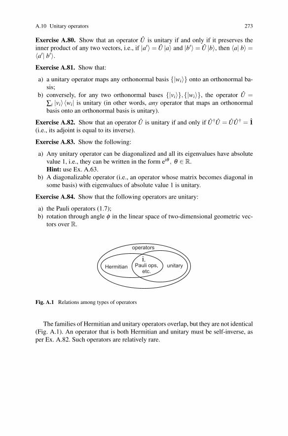
Fig. A.1 Relations among types of operators
The families of Hermitian and unitary operators overlap, but they are not identical(Fig. A.1). An operator that is both Hermitian and unitary must be self-inverse, asper Ex. A.82. Such operators are relatively rare.

274 A. I. Lvovsky. Quantum Physics
A.11 Functions of operators
The concept of function of an operator has many applications in linear algebra anddifferential equations. It is also handy in quantum mechanics, as operator functionspermit easy calculation of evolution operators.
Definition A.25. Consider a complex function f (x) defined on C. The function ofoperator f (A) of a diagonalizable operator A is the following operator:
f (A) = ∑i
f (ai) |ai〉〈ai| , (A.49)
where {|ai〉} is an orthonormal basis in which A diagonalizes:
A = ∑i
ai |ai〉〈ai| . (A.50)
Exercise A.85. Show that, if the vector |a〉 is an eigenvector of a Hermitian operatorA with eigenvalue a, then f (A) |a〉= f (a) |a〉.Exercise A.86. Suppose that the operator A is Hermitian and the function f (x),when applied to a real argument x, takes a real value. Show that f (A) is a Hermitianoperator, too.
Exercise A.88. Find the matrices of√
A and ln A in the orthonormal basis in which
A'(
1 33 1
)
Exercise A.89. Find the matrix of eiθ A, where A = 12
(1 11 1
).
Hint: One of the eigenvalues of A is 0, which means that the corresponding ei-genvector does not appear in the spectral decomposition (A.50) of A. However, theexponential of the corresponding eigenvalue is not zero, and the corresponding ei-genvectors do show up in the operator function (A.49).
Exercise A.90. Show that, for any operator A and function f , [A, f (A)] = 0.
Exercise A.91. Suppose f (x) has a Taylor decomposition f (x) = f0 + f1x+ f2x2 +. . .. Show that f (A) = f01+ f1A+ f2A2 + . . .
Exercise A.92. Show that, if the operator A is Hermitian, the operator eiA is unitary
and eiA =(
e−iA)−1
.
Exercise A.93.∗ Let ~s = (sx,sy,sz) be a unit vector (i.e. a vector of length 1). Showthat:
Exercise A.87. Suppose that the operator A is Hermitian and function f (x), whenapplied to any real argument x, takes a real non-negative value. Show that f (A) is anon-negative operator (see Defn. A.22).
A.11 Functions of operators 275
eiθ~s·~σ = cos θ 1+ i sin θ~s · ~σ , (A.51)
where ~σ = (σx, σy, σz),~s · ~σ = sxσx + syσy + szσz.Hint: There is no need find the explicit solutions for the eigenvectors of the operator~s · ~σ .
Exercise A.94.§ Find the matrices of the operators eiθσx , eiθσy , eiθσz in the canonicalbasis.Answer:
eiθσx =
(cosθ i sinθ
i sinθ cosθ
);
eiθσy =
(cosθ sinθ
−sinθ cosθ
);
eiθσz =
(eiθ 00 e−iθ
).
Definition A.26. Suppose the vector |ψ(t)〉 depends on a certain parameter t. Thederivative of |ψ(t)〉 with respect to t is defined as the vector
d |ψ〉dt
= lim∆ t→0
|ψ(t +∆ t)〉− |ψ(t)〉∆ t
. (A.52)
Similarly, the derivative of the operator Y (t) with respect to t is the operator
dYdt
= lim∆ t→0
Y (t +∆ t)− Y (t)∆ t
. (A.53)
Exercise A.95. Suppose that the matrix form of the vector |ψ(t)〉 is
|ψ(t)〉=
ψ1(t)...
ψN(t)
in some basis. Show that
d |ψ〉dt
=
dψ1(t)/dt...
dψN(t)/dt
.
Write an expression for the matrix form of an operator derivative.
Exercise A.96. Suppose the operator A is diagonalizable in an orthonormal basisand independent of t, where t is a real parameter. Show that d
dt eiAt = iAeiAt = ieiAt A.
276 A. I. Lvovsky. Quantum Physics
Exercise A.97.∗ For two operators A and B, suppose that [A, B] = ic1, where c is acomplex number. Prove the Baker-Hausdorff-Campbell formula
eA+B = eAeBe−ic/2 = eBeAeic/2 (A.54)
using the following steps.
a) Show that[A,eB] = ceB. (A.55)
Hint: use the Taylor series expansion for the exponential and Eq. (A.46).b) For an arbitrary number λ and operator G(λ ) = eλ Aeλ B, show that
dG(λ )
dλ= G(λ )(A+ B+λc) (A.56)
c) Solve the differential equation (A.56) to show that
G(λ ) = eλ A+λ B+λ 2c/2. (A.57)
d) Prove the Baker-Hausdorff-Campbell formula using Eq. (A.57).
This is a simplified form of the Baker-Hausdorff-Campbell formula. The full form of this formulais more complicated and holds for the case when [A, B] does not commute with A or B.
8
8
Appendix BProbabilities and distributions
B.1 Expectation value and variance
Definition B.1. Suppose a (not necessarily quantum) experiment to measure a quan-tity Q can yield any one of N possible outcomes {Qi} (1≤ i≤ N)}, with respectiveprobabilities pri. Then Q is called a random variable and the set of values {pri} forall values of i is called the probability distribution. The expectation (mean) value ofQ is
〈Q〉=N
∑i=1
priQi. (B.1)
Exercise B.1. Find the expectation of the value displayed on the top face of a fairdie.
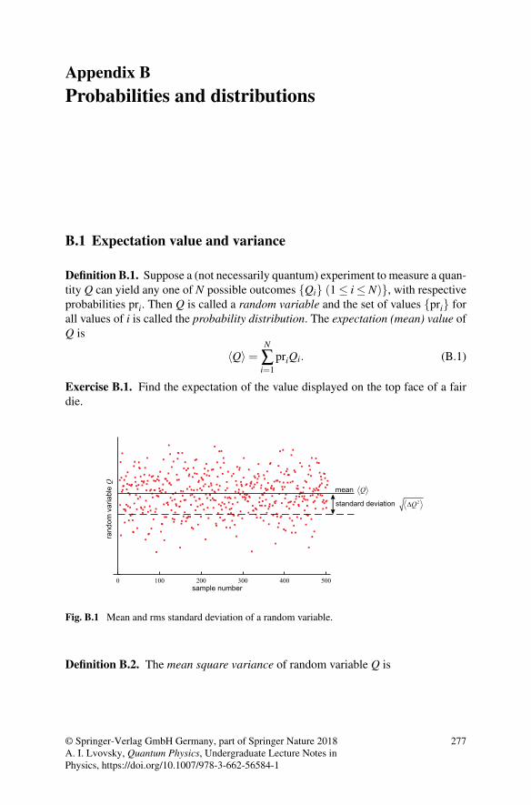
Fig. B.1 Mean and rms standard deviation of a random variable.
Definition B.2. The mean square variance of random variable Q is
A. I. Lvovsky, Quantum Physics, Undergraduate Lecture Notes inPhysics, https://doi.org/10.1007/978-3-662-56584-1
277
mean
standard deviation
sample number
ran
do
m v
aria
ble
Q
Q
Q2
0 100 200 300 400 500
© Springer-Verlag GmbH Germany, part of Springer Nature 2018

278 A. I. Lvovsky. Quantum Physics⟨∆Q2⟩= ⟨(Q−〈Q〉)2
⟩= ∑
ipri (Qi−〈Q〉)2 . (B.2)
The root mean square (rms) standard deviation, or uncertainty of Q is then√〈∆Q2〉.
While the expectation value, 〈Q〉=N∑
i=1priQi, shows the mean measurement out-
put, the statistical uncertainty shows by how much, on average, a particular measu-rement result will deviate from the mean (Fig. B.1).
Exercise B.2. Show that, for any random variable Q,⟨∆Q2⟩= ⟨Q2⟩−〈Q〉2 . (B.3)
Exercise B.3. Calculate the mean square variance of the value displayed on the topface of a fair die. Show by direct calculation that Eqs. (B.2) and (B.3) yield thesame.
Exercise B.4. Two random variables Q and R are independent, i.e., the realizationof one does not affect the probability distribution of the other (for example, a die anda coin being tossed next to each other). Show that 〈QR〉= 〈Q〉〈R〉. Is this statementvalid if Q and R are not independent?Hint: Independence means that events Qi and R j occur at the same time with pro-bability prQ
i prRj for each pair (i, j), where prQ
i is the probability of the i th value ofvariable Q and prR
j is the probability of the j th value of R.
Exercise B.5. Suppose a random variable Q is measured (for example, a die isthrown) N times. Consider the random variable Q that is the sum of the N outcomes.Show that the expectation and variance of Q equal⟨
Q⟩= N 〈Q〉
and ⟨∆ Q2⟩= N
⟨∆Q2⟩ ,
respectively.
B.2 Conditional probabilities
The conditional probability prA|B is the probability of some event A given that anot-her event, B, is known to have occurred. Examples are:
• the probability that the value on a die is odd given that it is greater than 3;• the probability that Alice’s HIV test result will be positive given that she is actu-
ally not infected;• the probability that Bob plays basketball given that he is a man and 185 cm tall;

B.2 Conditional probabilities 279
• the probability that it will rain tomorrow given that it has rained today.
Let us calculate the conditional probability using the third example. Event A is“Bob plays basketball”. Event B is “Bob is a 185-cm tall man”. The conditional pro-bability is equal to the number N(A and B) of 185-cm tall men who play basketballdivided by the number N(B) of 185-cm tall men [Fig. B.2(a)]:
prA|B =N(A and B)
N(B). (B.4)
Let us divide both the numerator and the denominator of the above fraction by N,the total number of people in town. Then we have in the numerator N(A and B)/N =prA and B — the probability that a randomly chosen person is a 185-cm tall man whoplays basketball, and in the denominator, N(B)/N = prB — the probability that arandom person is a 185-cm tall man. Hence
prA|B =prA and B
prB. (B.5)
This is a general formula for calculating conditional probabilities.
Exercise B.6. Suppose events B1, . . . ,Bn are mutually exclusive and collectivelyexhaustive, i.e., one of them must occur, but no two occur at the same time[Fig. B.2(b)]. Show that, for any other event A,
prA =n
∑i=1
prA|BiprBi
. (B.6)
This result is known as the theorem of total probability.
Fig. B.2 Conditional probabilities. a) Relation between the conditional and combined probabili-ties, Eq. (B.5). b) Theorem of total probability (Ex. B.6).
Exercise B.7. The probability that a certain HIV test gives a false positive result is
prpositive|not infected = 0.05.
The probability of a false negative result is zero. It is known that, of all people takingthe test, the probability of actually being infected is prinfected = 0.001.
a) b)
A
B
A BA
BB B
and
21 3
280 A. I. Lvovsky. Quantum Physics
a) What is the probability prpositive and not infected that a random person taking thetest is not infected and shows a false positive result?
b) What is the probability prpositive that a random person taking the test shows apositive result?
c) A random person, Alice, has been selected and the test has been performed onher. Her result turned out to be positive. What is the probability that she is notinfected?
Hint: To visualize this problem, imagine a city of one million. How many of themare infected? How many are not? How many positive test results will there be alltogether?
B.3 Binomial and Poisson distributions
Exercise B.8. A coin is tossed n times. Find the probability that heads will appeark times, and tails n− k times:
a) for a fair coin, i.e., the probability of getting heads or tails in a single toss is1/2;
b) for a biased coin, with the probabilities for the heads and tails being p and 1− p,respectively.Answer:
prk =
(nk
)pk(1− p)n−k. (B.7)
The probability distribution defined by Eq. (B.7) is called the binomial distribu-tion. We encounter this distribution in everyday life, often without realizing it. Hereare a few examples.
Exercise B.9.§
a) On a given day in a certain city 20 babies were born. What is the probabilitythat exactly nine of them are girls?
b) A student answers 3/4 of questions on average. What is the probability that(s)he scores perfectly on a 10-question test?
c) A certain politician has 60% electoral support. What is the probability that (s)hereceives more than 50% of the votes in a district with 100 voters?
Exercise B.10. Find the expectation value and the uncertainty of the binomial dis-tribution (B.7).Answer:
〈k〉= np;⟨∆k2⟩= np(1− p). (B.8)
Exercise B.11. In a certain big city, 10 babies are born per day on average. What isthe probability that on a given day, exactly 12 babies are born?
a) The city population is 100000.
B.4 Probability densities 281
b) The city population is 1000000.
Hint: Perhaps there is a way to avoid calculating 1000000!.
We see from the above exercise that in the limit p→ 0 and n→∞, but λ = pn =const, the probabilities in the binomial distribution become dependent on λ , ratherthan p and n individually. This important extension of the binomial distribution isknown as the Poisson (Poissonian) distribution.
Exercise B.12. Show that in the limit p→ 0 and n→ ∞, but λ = pn = const, thebinomial distribution (B.7) becomes
prk = e−λ λ k
k!(B.9)
using the following steps.
a) Show that limn→∞
1nk
(nk
)= 1
k! .
b) Show that limn→∞
(1− p)n−k = e−λ .c) Obtain Eq. (B.9).
Exercise B.13. Find the answer to Ex. B.11 in the limit of an infinitely large city.
Here are some more examples of the Poisson distribution.
Exercise B.14.§
a) A patrol policeman posted on a highway late at night has discovered that, onaverage, 60 cars pass every hour. What is the probability that, within a givenminute, exactly one car will pass that policeman?
b) A cosmic ray detector registers 500 events per second on average. What is theprobability that this number equals exactly 500 within a given second?
c) The average number of lions seen on a one-day safari is 3. What is the probabi-lity that, if you go on that safari, you will not see a single lion?
Exercise B.15. Show that both the mean and variance of the Poisson distribution(B.9) equal λ .
For example, in a certain city, 25 babies are born per day on average, so λ = 25.The root mean square uncertainty in this number
√λ = 5, i.e., on a typical day we
are much more likely to see 20 or 30 babies rather than 10 or 40 (Fig. B.3).Although the absolute uncertainty of n increases with 〈n〉, the relative uncertainty√
λ/λ decreases. In our example above, the relative uncertainty is 5/25 = 20%. Butin a smaller city, where 〈n〉= 4, the relative uncertainty is as high as 2/4 = 50%.
B.4 Probability densities
So far, we have studied random variables that can take values from a discrete set,with the probability of each value being finite. But what if we are dealing with

282 A. I. Lvovsky. Quantum Physics
10 20 30 40
0.05
0.10
0.15
n
prn
Fig. B.3 the Poisson distribution with 〈n〉= 4 (empty circles) and 〈n〉= 25 (filled circles).
a continuous random variable — for example, the wind speed, the decay time of aradioactive atom, or the range of a projectile? In this case, there is now way to assigna finite probability value to each specific value of Q. The probability that the atomdecays after precisely two milliseconds, or the wind speed is precisely five metersper second, is infinitely small.
However, the probability of detecting Q within some range — for example, thatthe atom decays between times 2 ms and 2.01 ms — is finite. We can thereforediscretize the continuous variable: divide the range of values that Q can take intoequal bins of width δQ. Then we define a discrete random variable Q with possiblevalues Qi equal to the central point of each bin, and the associated finite probabilityprQi
that Q falls within that bin [Fig. B.4(a,b)]. As for any probability distribution,∑i prQi
= 1. Of course, the narrower the bin width we choose, the more precisely wedescribe the behavior of the continuous random variable.
The probability values associated with neighboring bins can be expected to beclose to each other if the bin width is chosen sufficiently small. For atomic decay,for example, we can write pr[2.00 ms,2.01 ms]≈ pr[2.01 ms,2.02 ms]≈ 1
2 pr[2.00 ms,2.02 ms]. Inother words, for small bin widths, the quantity prQi
/δQ is independent of δQ. Hencewe can introduce the notion of the probability density or continuous probabilitydistribution1:
pr(Q) = limδQ→0
prQi(Q)
δQ, (B.10)
where i(Q) is the number of the bin within which the value of Q is located and the li-mit is taken over a set of discretized probability distributions for Q. This probabilitydensity is the primary characteristic of a continuous random variable.
Note also that, because the discrete probability prQi(Q) is a dimensionless quan-tity, the dimension of a continuous probability density pr(Q) is always the reciprocaldimension of the corresponding random variable Q.
1 Throughout this book, I use subscripts for discrete probabilities, such as in pri or prQi, and
parentheses for continuous probability densities, e.g., pr(Q).
B.4 Probability densities 283
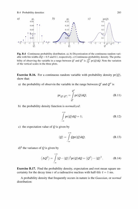
pri pr( )Qpri
�� �� �� � � � � �� �� �� � � � � �� �� �� � � � �
Qi Qi Q
����
����
����
����
���
���
����
���
����
���
���
���
���
���
��
a) b) c)
Q Q��
Fig. B.4 Continuous probability distribution. a), b) Discretization of the continuous random vari-able with bin widths δQ = 0.5 and 0.1, respectively. c) Continuous probability density. The proba-bility of observing the variable in a range between Q′ and Q′′ is
∫ Q′′
Q′ pr(Q)dQ. Note the variationof the vertical scales in the three plots.
Exercise B.16. For a continuous random variable with probability density pr(Q),show that:
a) the probability of observin the variable in the range between Q′ and Q′′ is
pr[Q′,Q′′] =Q′′∫
Q′
pr(Q)dQ; (B.11)
b) the probability density function is normalized:
+∞∫−∞
pr(Q)dQ = 1; (B.12)
c) the expectation value of Q is given by
〈Q〉=+∞∫−∞
Qpr(Q)dQ; (B.13)
d)§ the variance of Q is given by
⟨∆Q2⟩= +∞∫
−∞
(Q−〈Q〉)2pr(Q)dQ =⟨Q2⟩−〈Q〉2 . (B.14)
Exercise B.17. Find the probability density, expectation and root mean square un-certainty for the decay time t of a radioactive nucleus with half-life τ = 1 ms.
A probability density that frequently occurs in nature is the Gaussian, or normaldistribution:
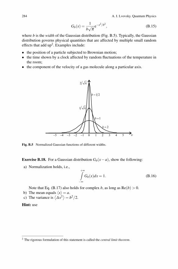
284 A. I. Lvovsky. Quantum Physics
Gb(x) =1
b√
πe−x2/b2
, (B.15)
where b is the width of the Gaussian distribution (Fig. B.5). Typically, the Gaussiandistribution governs physical quantities that are affected by multiple small randomeffects that add up2. Examples include:
• the position of a particle subjected to Brownian motion;• the time shown by a clock affected by random fluctuations of the temperature in
the room;• the component of the velocity of a gas molecule along a particular axis.
Fig. B.5 Normalized Gaussian functions of different widths.
Exercise B.18. For a Gaussian distribution Gb(x−a), show the following:
a) Normalization holds, i.e.,+∞∫−∞
Gb(x)dx = 1. (B.16)
Note that Eq. (B.17) also holds for complex b, as long as Re(b)> 0.b) The mean equals 〈x〉= a.c) The variance is
⟨∆x2
⟩= b2/2.
Hint: use
2 The rigorous formulation of this statement is called the central limit theorem.
1
2
b 1 2
x

B.4 Probability densities 285
+∞∫−∞
e−x2/b2dx = b
√π; (B.17)
+∞∫−∞
x2e−x2/b2dx =
b3√π
2. (B.18)

Appendix COptical polarization tutorial
C.1 Polarization of light
Consider a classical electromagnetic plane wave propagating along the (horizontal)z-axis with angular frequency ω and wavenumber k = ω/c, where c is the speed oflight. The electromagnetic wave is transverse, so its electric field vector lies in thex-y plane:
~E(z, t) = AH icos(kz−ωt +ϕH)+AV j cos(kz−ωt +ϕV ), (C.1)
or in the complex form
~E(z, t) = Re[(AHeiϕH i+AV eiϕV j)eikz−iωt ]. (C.2)
Here i and j are unit vectors along the x and y axes, respectively; AH and AV are thereal amplitudes of the x and y components (which we will refer to as horizontal andvertical), and ϕH and ϕV are their phases.
Exercise C.1.§ Show that Eqs. (C.1) and (C.2) are equivalent.
The intensity of light in each polarization is proportional to:
IH ∝ A2H ; (C.3a)
IV ∝ A2V . (C.3b)
The total intensity of the wave is the sum of its two components: Itotal ∝ A2H +A2
V .Let us study the behavior of the electric field vector at some specific point in
space, say z= 0. If the two components of the field have different phases, ~E(z, t) willchange its direction as a function of time, as illustrated in Fig. C.1. To understandthis interesting phenomenon better, try the following exercise.
Exercise C.2. Plot, as a function of time, the horizontal and vertical components of~E(0, t) for 0≤ ωt ≤ 2π , in the following cases:
a) AH = 1 V/m, AV = 0, ϕH = ϕV = 0;
A. I. Lvovsky, Quantum Physics, Undergraduate Lecture Notes inPhysics, https://doi.org/10.1007/978-3-662-56584-1
287© Springer-Verlag GmbH Germany, part of Springer Nature 2018
288 A. I. Lvovsky. Quantum Mechanics I.
x
y
z tor
horizontalcomponent
verticalcomponent
polarizationpattern
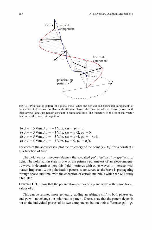
Fig. C.1 Polarization pattern of a plane wave. When the vertical and horizontal components ofthe electric field vector oscillate with different phases, the direction of that vector (shown withthick arrows) does not remain constant in phase and time. The trajectory of the tip of that vectordetermines the polarization pattern.
b) AH = 5 V/m, AV =−3 V/m, ϕH = ϕV = 0;c) AH = 5 V/m, AV =−3 V/m, ϕH = π/2, ϕV = 0;d) AH = 5 V/m, AV =−3 V/m, ϕH = π/4, ϕV =−π/4;e) AH = 5 V/m, AV =−3 V/m, ϕH = 0, ϕV = π/6.
For each of the above cases, plot the trajectory of the point (Ex,Ey) for a constant zas a function of time.
The field vector trajectory defines the so-called polarization state (pattern) oflight. The polarization state is one of the primary parameters of an electromagne-tic wave; it determines how this field interferes with other waves or interacts withmatter. Importantly, the polarization pattern is conserved as the wave is propagatingthrough space and time, with the exception of certain materials which we will studya bit later.
Exercise C.3. Show that the polarization pattern of a plane wave is the same for allvalues of z.
This can be restated more generally: adding an arbitrary shift to both phases ϕHand ϕV will not change the polarization pattern. One can say that the pattern dependsnot on the individual phases of its two components, but on their difference ϕH −ϕV
C.2 Polarizing beam splitter 289
[see Ex. C.2(c,d) for an example]. This property of classical polarization patternshas a direct counterpart in the quantum world: applying an overall phase shift toa quantum state does not change its physical properties (see Sec. 1.3 for a moredetailed discussion).
In general, the polarization pattern is elliptical; however, as we have seen above,there exist special cases when the ellipse collapses into a straight line or blows outinto a circle. Let us look at these cases more carefully.
Exercise C.4. Show the following:
a) The polarization pattern is linear if and only if ϕH = ϕV +mπ , where m is aninteger, or AH = 0 or AV = 0. The angle θ of the field vector with respect to thex axis is given by tanθ = AV/AH .
b) The polarization pattern is circular if and only if ϕH = ϕVπ
2 +mπ , where m isan integer, and AH =±AV .
Important specific cases of linear polarization are horizontal (AV = 0), vertical(AH = 0), and±45◦ (AV =±AH ). For circular polarization, one can distinguish twocases according to the helicity of the wave: right and left circular.
• For right circular polarization, AV = AH and ϕV = ϕH + π
2 +2πm or AV =−AHand ϕV = ϕH − π
2 +2πm, where m is an integer.• For left circular polarization, AV = AH and ϕV = ϕH − π
2 + 2πm or AV = −AH
and ϕV = ϕH + π
2 +2πm, where m is an integer1.
Exercise C.5.∗ Show that, when none of the conditions of Ex. C.4 are satisfied, thetip of the electric field vector follows an elliptical pattern.
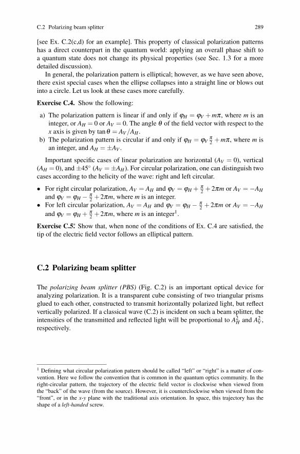
C.2 Polarizing beam splitter
The polarizing beam splitter (PBS) (Fig. C.2) is an important optical device foranalyzing polarization. It is a transparent cube consisting of two triangular prismsglued to each other, constructed to transmit horizontally polarized light, but reflectvertically polarized. If a classical wave (C.2) is incident on such a beam splitter, theintensities of the transmitted and reflected light will be proportional to A2
H and A2V ,
respectively.
1 Defining what circular polarization pattern should be called “left” or “right” is a matter of con-vention. Here we follow the convention that is common in the quantum optics community. In theright-circular pattern, the trajectory of the electric field vector is clockwise when viewed fromthe “back” of the wave (from the source). However, it is counterclockwise when viewed from the“front”, or in the x-y plane with the traditional axis orientation. In space, this trajectory has theshape of a left-handed screw.
290 A. I. Lvovsky. Quantum Mechanics I.
polarizing
beam splitterhorizontal
polarization
vertical
polarization
Fig. C.2 Polarizing beam splitter.
C.3 Waveplates
It is sometimes necessary to change the polarization state of light without splittingthe vertical and horizontal components spatially. This is normally achieved usingan optical instrument called a waveplate. The waveplate relies on birefringence,or double refraction — an optical property displayed by certain materials, prima-rily crystals, for example quartz or calcite. Birefringent crystals have an anisotropicstructure, such that a light wave propagating through them will not conserve its pola-rization pattern unless it is linearly polarized along one of the two directions: eitheralong or perpendicular to the crystal’s optic axis. Traditionally, these directions arereferred to as extraordinary and ordinary, respectively.
A birefringent material exhibits different indices of refraction for these two pola-rizations. Therefore, after propagation through the crystal, the ordinary and extraor-dinary waves will acquire different phases: ∆ϕe and ∆ϕo, respectively. Because anoverall phase shift has no effect on the polarization pattern, the quantity of interestis the difference δϕ = ∆ϕe−∆ϕo.
Exercise C.6. The indices of refraction for light polarized along and perpendicularto the optic axis are ne and no, respectively, the length of the crystal is L, and thewavelength in vacuum is λ . Find δϕ .
A waveplate is a birefringent crystal of a certain length, so ∆ϕ is preciselyknown. Two kinds of waveplates are manufactured commercially: λ/2-plate (half-wave plate) with δϕ = π and λ/4-plate (quarter-wave plate) with δϕ = π/2.
If the polarization pattern is not strictly ordinary or extraordinary, propagationthrough a birefringent crystal will transform it. In order to determine this transfor-mation, we decompose the wave into the extraordinary and ordinary components.The phase shift of each component is known. Knowing the new phases of both com-ponents, we can combine them to find the new polarization pattern.
Exercise C.7. For each of the polarization states of Ex. C.2, plot the polarizationpatterns that the waves will acquire when they propagate through (a) a half-waveplate, (b) a quarter-wave plate with the optical axes oriented vertically.
Solving the above exercise, you may have noticed that the half-wave plate “flips”the polarization pattern around the vertical (or horizontal) axis akin to a mirror.
C.3 Waveplates 291
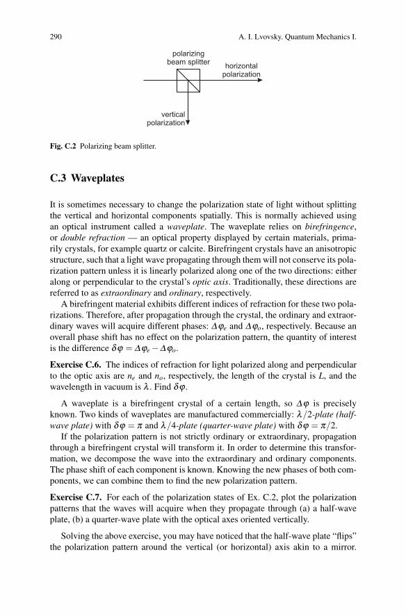
x
y
z
Fig. C.3 Action of a λ/2-plate with optic axis oriented vertically. Different refractive indices forthe ordinary and extraordinary polarizations result in different optical path lengths, thereby rotatingthe polarization axis.
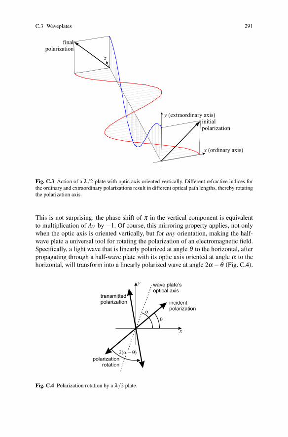
This is not surprising: the phase shift of π in the vertical component is equivalentto multiplication of AV by −1. Of course, this mirroring property applies, not onlywhen the optic axis is oriented vertically, but for any orientation, making the half-wave plate a universal tool for rotating the polarization of an electromagnetic field.Specifically, a light wave that is linearly polarized at angle θ to the horizontal, afterpropagating through a half-wave plate with its optic axis oriented at angle α to thehorizontal, will transform into a linearly polarized wave at angle 2α−θ (Fig. C.4).
Fig. C.4 Polarization rotation by a λ/2 plate.
(ordinary axis)
(extraordinary axis)initialpolarization
finalpolarization
incident polarization
wave plate’soptical axis
transmitted polarization
polarizationrotation
y
x
a
q
2(a - q)
292 A. I. Lvovsky. Quantum Mechanics I.
Exercise C.8.§ Show that a λ/2-plate with the optic axis oriented at 22.5◦ to thehorizontal interconverts between the horizontal and 45◦ polarizations, as well asbetween the vertical and −45◦ polarizations.
However, rotations alone do not provide a full set of possible transformations. Forexample, half-wave plates cannot transform between linear and circular/ellipticalpatterns. To accomplish this, we would need a quarter-wave plate.
Exercise C.9. Show that a λ/4-plate with the optic axis oriented horizontally orvertically interconverts between the circular and ±45◦ polarizations.
Exercise C.10. Linearly polarized light at angle θ to the horizontal propagatesthrough a λ/4-plate with the optic axis oriented vertically. For the resulting ellipti-cal pattern, find the angle between the major axis and the horizontal and the ratio ofthe minor to major axes.
Exercise C.11.∗ Suppose you have a source of horizontally polarized light. Showthat, by using one half-wave plate and one quarter-wave plate, you can obtain lightwith an arbitrary polarization pattern.Hint: It is easier to tackle this problem using geometric arguments, particularly theresult of Ex. C.5, rather than formal algebra.
Exercise C.12.∗ Linearly polarized light propagates through a half-wave plate, thenthrough a quarter-wave plate at angle 45◦ to the horizontal, then through a polarizingbeam splitter. Show that the transmitted intensity does not depend on the angle ofthe half-wave plate.

Appendix DDirac delta function and the Fouriertransformation
D.1 Dirac delta function
The delta function can be visualized as a Gaussian function (B.15) of infinitelynarrow width b (Fig. B.5):
Gb(x) =1
b√
πe−x2/b2 → δ (x) for b→ 0. (D.1)
The delta function is used in mathematics and physics to describe density distri-butions of infinitely small (singular) objects. For example, the position-dependentdensity of a one-dimensional particle of mass m located at x = a, can be written asmδ (x−a). Similarly, the probability density of a continuous “random variable” thattakes on a certain value x = a is δ (x−a). In quantum mechanics, we use δ (x), forexample, to write the wave function of a particle that has a well-defined position.
The notion of function in mathematics refers to a map that relates a number, x,to another number, f (x). The delta function is hence not a function in the traditionalsense: it maps all x 6= 0 to zero, but x= 0 to infinity, which is not a number. It belongsto the class of so-called generalized functions. A rigorous mathematical theory ofgeneralized functions can be found in most mathematical physics textbooks. Here,we discuss only those properties of the delta function that are useful for physicists.
Exercise D.1. Show that, for any smooth1, bounded function f (x),
limb→0
+∞∫−∞
Gb(x) f (x)dx = f (0). (D.2)
From Eqs. (D.1) and (D.2) and for any smooth function f (x), we obtain
1 A smooth function is one that has derivatives of all finite orders.
A. I. Lvovsky, Quantum Physics, Undergraduate Lecture Notes inPhysics, https://doi.org/10.1007/978-3-662-56584-1
293© Springer-Verlag GmbH Germany, part of Springer Nature 2018

294 A. I. Lvovsky. Quantum Physics
+∞∫−∞
δ (x) f (x)dx = f (0) (D.3)
This property is extremely important because it allows one to perform meaning-ful calculations with the delta function in spite of its singular nature. Although thedelta function does not have a numerical value for all values of its argument, theintegral of the delta function multiplied by another function does. We may write adelta function outside of an integral, but we always keep in mind that it will eventu-ally become a part of an integral, and only then will it produce a quantitative value— for example, a prediction of an experimental result.
In fact, Eq. (D.3) can be viewed as a rigorous mathematical definition of the deltafunction. Using this definition, we can obtain its other primary properties.
Exercise D.2. Show that
a)+∞∫−∞
δ (x)dx = 1; (D.4)
b) for any function f (x),
+∞∫−∞
δ (x−a) f (x)dx = f (a); (D.5)
c) for any real number a,δ (ax) = δ (x)/|a|. (D.6)
Exercise D.3. For the Heaviside step function
θ(x) ={
0 if x < 01 if x≥ 0
, (D.7)
show thatddx
θ(x) = δ (x). (D.8)
Hint: use Eq. (D.3).
Exercise D.4. Show that, for any c < 0 and d > 0,
d∫c
δ (x)dx = 1 (D.9)

D.2 Fourier transformation 295
D.2 Fourier transformation
Definition D.1. The Fourier transform f (k) ≡ F [ f ](k) of a function f (x) is afunction of the parameter k defined as follows:2
f (k) =1√2π
+∞∫−∞
e−ikx f (x)dx. (D.10)
This is an important integral transformation used in all branches of physics. Sup-pose, for example, that you have a light wave of the form f (ω)e−iωt , where ω is thefrequency and f (ω) is the complex amplitude, or the frequency spectrum of the sig-
nal. Then the time-dependent signal from all sources is+∞∫−∞
f (ω)e−iωtdω — that is,
the Fourier transform of the spectrum. The power density of the spectrum, i.e., thefunction | f (ω)|2, can be measured experimentally by means of a dispersive opticalelement, such as a prism.
Exercise D.5. Show that, if f (k) = F [ f (x)] exists, then
a)
f (0) =1√2π
+∞∫−∞
f (x)dx; (D.11)
b) for a real f (x), f (−k) = f ∗(k);c) for a 6= 0,
F [ f (ax)] =1|a|
f (k/a); (D.12)
d)F [ f (x−a)] = e−ika f (k); (D.13)
e)F [eiξ x f (x)] = f (k−ξ ); (D.14)
f) assuming that f (x) is a smooth function approaching zero at ±∞,
F [d f (x)/dx] = ik f (k). (D.15)
Exercise D.6. Show that the Fourier transform of a Gaussian function is also aGaussian function:
F [e−x2/b2] =
b√2
e−k2b2/4. (D.16)
We see from Eq. (D.12) that scaling the argument x of a function results in in-verse scaling of the argument k of its Fourier transform. In particular (Ex. D.6), a
2 There is no common convention as to whether to place the negative sign in the complex exponentof Eqs. (D.10) or (D.21), nor how to distribute the factor of 1/2π between them. Here I have chosenthe convention arbitrarily.
296 A. I. Lvovsky. Quantum Physics
signal with a Gaussian spectrum of width b is a Gaussian pulse of width 2/b, so theproduct of the two widths is a constant. This is a manifestation of the time-frequencyuncertainty that applies to a wide range of wave phenomena in classical physics. Infact, as we see in Sec. 3.3.2, in its application to the position and momentum obser-vables, the Heisenberg uncertainty principle can also be interpreted in this fashion.
Let us now consider two extreme cases of the Fourier transform of Gaussianfunctions.
Exercise D.7. Show that:
a) in the limit b→ 0, Eq. (D.16) takes the form
F [δ (x)] =1√2π
; (D.17)
b) in the opposite limit, b→ ∞, one obtains
F [1] =√
2π δ (k). (D.18)
If the spectrum contains only the zero frequency, the signal, not surprisingly,is time-independent. If, on the other hand, the spectrum is constant, the signal isan instant “flash” occurring at t = 0. Here is an interesting consequence of thisobservation.
Exercise D.8. Show that, for a 6= 0,
+∞∫−∞
eiakxdx = 2πδ (k)/|a|. (D.19)
This result is of paramount importance for many calculations involving the Fou-rier transform. We will see its utility shortly.
Exercise D.9. Assuming a and b to be real and positive, find the Fourier transformsof the following:
a) δ (x+a)+δ (x−a)b) cos(ax+b);c) e−ax2
cosbx;d) e−a(x+b)2
+ e−a(x−b)2;
e) θ(x)e−ax, where θ(x) is the Heaviside function;
f) a “top-hat function”{
0 if x <−a or x > a;A if −a≤ x≤ a; .
The Fourier transform can be inverted: for any given time-dependent pulse onecan calculate its frequency spectrum such that the pulse is the Fourier transformof that spectrum. Remarkably, the Fourier transform is very similar to its inverse.This similarity can be observed, for example, by comparing Eqs. (D.13) and (D.14).Displacing the argument of f (x) leads to the multiplication of f (k) by a complex
D.2 Fourier transformation 297
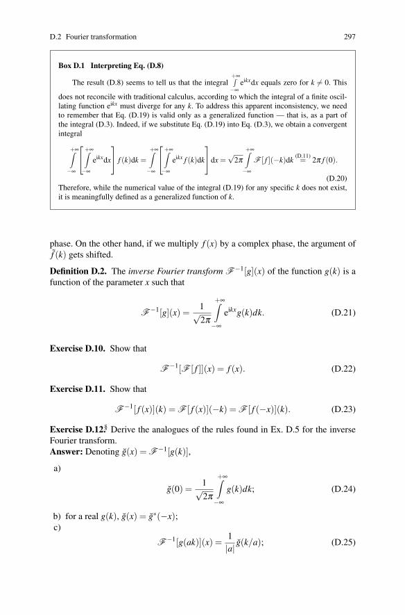
Box D.1 Interpreting Eq. (D.8)
The result (D.8) seems to tell us that the integral+∞∫−∞
eikxdx equals zero for k 6= 0. This
does not reconcile with traditional calculus, according to which the integral of a finite oscil-lating function eikx must diverge for any k. To address this apparent inconsistency, we needto remember that Eq. (D.19) is valid only as a generalized function — that is, as a part ofthe integral (D.3). Indeed, if we substitute Eq. (D.19) into Eq. (D.3), we obtain a convergentintegral
+∞∫−∞
+∞∫−∞
eikxdx
f (k)dk =+∞∫−∞
+∞∫−∞
eikx f (k)dk
dx =√
2π
+∞∫−∞
F [ f ](−k)dk(D.11)= 2π f (0).
(D.20)Therefore, while the numerical value of the integral (D.19) for any specific k does not exist,it is meaningfully defined as a generalized function of k.
phase. On the other hand, if we multiply f (x) by a complex phase, the argument off (k) gets shifted.
Definition D.2. The inverse Fourier transform F−1[g](x) of the function g(k) is afunction of the parameter x such that
F−1[g](x) =1√2π
+∞∫−∞
eikxg(k)dk. (D.21)
Exercise D.10. Show that
F−1[F [ f ]](x) = f (x). (D.22)
Exercise D.11. Show that
F−1[ f (x)](k) = F [ f (x)](−k) = F [ f (−x)](k). (D.23)
Exercise D.12.§ Derive the analogues of the rules found in Ex. D.5 for the inverseFourier transform.Answer: Denoting g(x) = F−1[g(k)],
a)
g(0) =1√2π
+∞∫−∞
g(k)dk; (D.24)
b) for a real g(k), g(x) = g∗(−x);c)
F−1[g(ak)](x) =1|a|
g(k/a); (D.25)
298 A. I. Lvovsky. Quantum Physics
d)F−1[g(k−a)](x) = eixag(k); (D.26)
e)F−1[eiξ kg(k)](x) = g(x+ξ ); (D.27)
f)F−1[dg(k)/dk] =−ixg(x). (D.28)

Index
Angstrom, Anders Jonas, 193
adiabatic theorem, 71adjoint
operator, 268space, 261vector, 47, 261
ammonia maser, 119amplitude, 257angular momentum
commutation relations, 175, 179definition, 174differential form
in Cartesian coordinates, 175in spherical coordinates, 177
eigenvalues and eigenstates, 178matrix form, 178raising and lowering operators, 179
annihilation operator, 132Aspect, Alain, 64atomic clock, 215
Baker-Hausdorff-Campbell formula, 275Balmer, Johann Jakob, 193basis, 257
canonical, 6, 42, 181orthonormal, 259
decomposing into, 260BB84 (quantum cryptography protocol), 19beam splitter, 14Beer’s law, 21Bell inequality, 59Bell, John, 59bipartite states, 41Bloch
sphere, 198vector, 198, 236
of a mixed state, 231relaxation, 236
Bloch, Felix, 198Bogoliubov transformation, 156Bogoliubov, Nikolay Nikolayevich, 156Bohm, David, 57Bohr
magneton, 202model of hydrogen atom, 191radius, 188
Bohr’s model of hydrogen atom, 193Bohr, Niels, 100, 191, 202Boltzmann, Ludwig, 196bomb paradox, 15, 73Born’s rule, 10, 222, 241Born, Max, 10, 71bosons, 136, 186bound state, 114
c-not gate, 81c-phase gate, 81Cauchy-Schwarz inequality, 261causality, 50Clauser, John, 64coherence, 17, 49, 56, 69, 224, 225collapse, 10, 67commutator, 30, 271
angular momentum components, 175, 179position and momentum, 105, 131
Compton, Arthur, 5conditional phase gate, 81conditional-not gate, 81continuous observables, 93Copenhagen interpretation, 66correspondence principle, 2creation operator, 132cryptography
A. I. Lvovsky, Quantum Physics, Undergraduate Lecture Notes inPhysics, https://doi.org/10.1007/978-3-662-56584-1
299© Springer-Verlag GmbH Germany, part of Springer Nature 2018
300 Index
private-key, 18public-key, 18quantum, 19
error rate, 20
de Broglie wave, 32, 99three-dimensional, 170
de Broglie, Louis, 100decoherence, 69, 111, 231, 233
preferred basis, 70, 231, 233degree of degeneracy, 180delta function, 94, 293
potentialdouble, 119single, 118
density operator/matrix, 222diagonal and off-diagonal elements, 225reduced, 230
dephasing, see decoherencehomogeneous, 233inhomogeneous, 213longitudinal and transverse, 237
detection loophole, 63determinism, 10dimension (of a linear space), 257Dirac
delta function, see delta functionnotation, 255, 262
Dirac, Paul, 255, 293displacement operator, 148, 152
efficiency, see photon detector, quantumefficiency
Ehrenfest theorem, 145Ehrenfest, Paul, 145Einstein, Albert, vii, 5, 10, 57, 106, 158, 175,
209Einstein–Podolsky–Rosen paradox, 57
for continuous variables, 106, 158energy levels, 114ensemble, 13, 56, 212, 221entanglement, 42
swapping, 85EPR paradox, see Einstein–Podolsky–Rosen
paradoxEverett, Hugh, 73evolution
in Heisenberg picture, 143of density matrices, 226of magnetic states, 204of probability densities, 150operator, 33
expectation value, see mean value
Fabry-Perot etalon, 129faster-than-light communications, see
superluminal signallingfermions, 136, 186Feynman, Richard, 69Fock states, 134Fock, Vladimir Aleksandrovich, 71, 134force, 145, 203Fourier transform, 295
inverse, 297free induction decay, 212Fresnel, Augustin-Jean, 123function of an operator, 274
Gaussian distribution, 283Gaussian wavepacket, 159Gedankenexperiment, 10GHZ nonlocality, 63Glauber, Roy, 139God does not play dice, 10, 68Gram-Schmidt procedure, 260Greenberger–Horne–Zeilinger nonlocality, 63ground state, 196group velocity, 110gyromagnetic ratio, 200, 201
harmonic oscillator, 129Heisenberg picture, 144, 204, 226Heisenberg’s equation, 144Heisenberg, Werner, 31, 105, 144heralded photon, 24, 138hidden parameters, 58Hilbert space, 259
Postulate, 3radial and angular, 174rigged, 94
Holevo bound, 48Holevo, Alexander Semenovich, 48, 243homodyne detector, 138, 160homogeneous dephasing, 233hydrogen atom
Bohr’s model, 191, 193energy spectrum, 190radial wavefunctions, 189
incompatible states, 3inhomogeneous broadening, 213inner product, 258
in tensor product space, 42partial, 52
intensity, 287interaction lifts degeneracy, 119
Lande factor, 200
Index 301
Landau, Lev Davidovich, 222Larmor frequency, 201, 202Larmor, Joseph, 201length of vector, see normLevi-Civita symbol, 174linear
independence, 256operator, 262space, 255
localhidden variables, 58measurement, 49, 53operator (in a tensor product space), 47realism, 57
localityloophole, 62principle, 57
lowering operator (angular momentum), 179Lyman, Theodore, 193
magneticquantum number, 180resonance, 206, 233
many-worlds interpretation, 73maser, 119master equations, 226matrix form
operator, 264adjoint, 268basis change, 266
state, 257vector, 257
mean value, 29, 277measurement
basis, 9generalized, 238local, 49, 53, 230of an observable, 27projective, 9, 228von Neumann, 67, 231
Measurement Postulate, 8for density matrices, 228for continuous observables, 97for local measurements, 53
Mendeleev, Dmitri Ivanovich, 194mixed state, 13, 17, 55, 69, 138, 223
Naimark, Mark Aronovich, 243Neumark’s (Naimark’s) theorem, 243no-cloning theorem, 46, 55Noether, Emmy, 176nonlocality, 57norm, 259number operator, 133
observable, 27operator
adjoint, 268commutation, 263, 271creation and annihilation, 132derivative of, 275diagonalization, 269displacement, 148, 152eigen
basis, 27, 269value, 27, 269vector/state, 27, 269
evolution, 33function of, 274Hadamard, 26Hermitian, 28, 268
tensor product, 47identity, 263linear, 262local (in a tensor product space), 47matrix, 264
basis change, 266number, 133phase shift, 153product, 263projection, 26, 228, 240raising and lowering (angular momentum),
179spectral decomposition, 28, 269squeezing, 154tensor product, 45unitary, 34, 273
tensor product, 47optical table, 12orbital quantum number, 180orthogonal states/vectors, 259outer product, 265overlap, 258
parametric down-conversion, 16, 24, 43, 160partial
inner product, 52trace, 230
Paschen, Friedrich, 193Pauli
exclusion principle, 186matrices, 26, 28, 182
Pauli, Wolfgang, 186, 191periodic table, 194phase
coherent, 139factor, 7, 141, 259
overall, 7, 10, 197shift operator, 153

302 Index
space, 130velocity, 110
phonon, 135photon, 5, 135, 136photon detector
click, 9, 22dark counts, 11, 22non-discriminating, 11, 240quantum efficiency, 11, 22, 240
Planck constant, 5, 32Planck, Max, 5, 32Poisson distribution, 24, 142, 281polarization
pattern, 289state
classical, 289measurement, 9
polarizing beam splitter, 8, 289position and momentum, 93
basis change, 100, 102rescaling, 131
positive operator-valued measure, 240postselection, 55Postulate
Hilbert space, 3Measurement, see Measurement Postulate
potentialbarrier, 125free space, 108step, 121well, 114
delta-function, 118well or barrier, transmission resonance, 129
POVM, 240power broadening, 210principal quantum number, 190principle of minimum energy, 196probability
conditional, 278density current, 123density, continuous, 282
quantum, 98distribution, 277
binomial, 280Poisson, 24, 142, 281
projection operator, 26, 228, 240pulse area, 211pure state, 223purity, 228, 232
quantize, 114, 200quantum
bit, 7, 79, 198cloning, 46, 55
computer, 79cryptography, 17dense coding, 48master equation, 226nonlocality, 57number
magnetic, 180orbital, 180principal, 190spin, 186
process, 245tensor, 247
repeater, 23, 86teleportation, 82tomography
detector, 249process, 245state, 14, 243, 244
quantum (noun), 135quantum measurement, see measurementqubit, see quantum bit
Rabi oscillations, 210Rabi, Isaak Isidor, 208radial equation, 178
hydrogen atom, 187raising operator (angular momentum), 179Ramsey spectroscopy, 215random variable, 277
continuous, 281reality (EPR paradox), 57reduced mass, 190relaxation, 215, 233
longitudinal and transverse, 237remote state preparation, 50resolution of the identity, 266resonance, 206rotating basis, 207rotating-wave approximation, 207Rutherford, Ernest, 191Rydberg
atoms, 194constant, 190
Rydberg’s formula, 193Rydberg, Johannes, 190, 193
saturation of a two-level system, 210scalar product, see inner productSchrodinger
cat, 4, 72equation, 34
for density matrices, 226three-dimensional, 171time-independent, 111

Index 303
picture, 144Schrodinger, Erwin, 4, 34, 144second quantization, 136shell, atomic, 196shoes, 49, 58Shut up and calculate, vi, 69, 79single-photon interference, 14spanning set, 257special relativity, 2, 50spectral theorem, 269spin, 186
echo, 213, 237quantum number, 186
spontaneous parametric down-conversion, seeparametric down-conversion
spreading of wavepackets, 111squeezing
single-mode, 154two-mode, 156
statebound, 114coherent, 139
evolution, 142wavefunction of, 140
entangled, 41Fock, 134ground, 196mixed, 13, 17, 55, 69, 138, 223pure, 223separable, 41squeezed, 154
photon-number decomposition, 159stationary, 33superposition, 4unbound, 120unnormalized, 26, 53, 222vacuum (harmonic oscillator), 134
statistical ensemble, see ensembleStern, Otto and Gerlach, Walther, 203Stern–Gerlach apparatus, 203subspace, 178, 258, 271superluminal signalling, 50, 126
teleportation, 82tensor product
operator, 45
space, 41adjoint, 47
theorem of total probability, 279thermalization, 235Thomson, J. J., 191time reversibility, 34, 231, 238time-independent Schrodinger equation, 111tomography, see quantum tomographyTownes, Charles, 119trace, 227
chain rule, 228partial, 230
transcendental equation, 115triangle inequality, 261tunnelling, 125two-level system, 206
unbound state, 120uncertainty, 278
principle, 1, 31, 183for position and momentum, 105
unit vector, 274unitary operator, see operator, unitary
vacuum state (harmonic oscillator), 134von Neumann measurement, 67von Neumann, John, 67, 222, 231
wave–particle duality, 17, 99wavefunction, 94
continuity conditions, 118of coherent state, 140of Fock states, 135of hydrogen atom, 187
radial, 189wavenumber, 101wavepacket, 101, 105, 109, 123waveplate, 289
operators, 25Welcher-Weg, 14Wigner’s friend, 68Wigner, Eugene, 68Wineland, David, 64
Zeilinger, Anton, 63, 64zero-point vibration, 134, 155