Towards Usable and Lean Parallel Linear Algebra Libraries
26
Transcript of Towards Usable and Lean Parallel Linear Algebra Libraries

Towards Usable and LeanParallel Linear Algebra Libraries �Almadena Chtchelkanova Carter EdwardsJohn Gunnels Greg MorrowJames Overfelt Robert van de Geijn yDepartment of Computer SciencesandTexas Institute for Computational and Applied MathematicsThe University of Texas at AustinAustin, Texas 78712May 1, 1996AbstractIn this paper, we introduce a new parallel library e�ort, as part of the PLAPACKproject, that attempts to address discrepencies between the needs of applications andparallel libraries. A number of contributions are made, including a new approachto matrix distribution, new insights into layering parallel linear algebra libraries, andthe application of \object based" programming techniques which have recently becomepopular for (parallel) scienti�c libraries. We present an overview of a prototype library,the SL Library, which incorporates these ideas. Preliminary performance data showsthis more application-centric approach to libraries does not necessarily adversely impactperformance, compared to more traditional approaches.�This project is sponsored in part by the O�ce of Naval Research under Contract N00014-95-1-0401,the NASA High Performance Computing and Communications Program's Earth and Space Sciences Projectunder NRA Grant NAG5-2497, the PRISM project under ARPA grant P-95006.yCorresponding and presenting author. Dept. of Computer Sciences, The University of Texas at Austin,Austin, TX 78712, (512) 471-9720 (O�ce), (512) 471-8885 (Fax), [email protected]
1 IntroductionDesign of parallel implementations of linear algebra algorithms and libraries traditionallystarts with the partitioning and distribution of matrices to the nodes (processors) of a dis-tributed memory architecture1. It is this partitioning and distribution that then dictates theinterface between an application and the library.While this appears to be convenient for the library, this approach creates an inherentcon ict between the needs of the application and the library. It is the vectors in linearsystems that naturally dictate the partitioning and distribution of work associated with(most) applications that lead to linear systems. Notice that in a typically application, thelinear system is created to compute values for degrees of freedom, which have some spatialsigni�cance. In �nite element or boundary element methods, we solve for force, stress, ordisplacement at points in space. For the application, it is thus more natural to partitionthe domain of interest into subdomains, like domain decomposition methods do, and assignthose subdomains to nodes. This is equivalent to partitioning the vectors and assigning thesubvectors to nodes.In this paper, we describe a parallel linear algebra library development e�ort, the PLA-PACK project at the University of Texas at Austin, that starts by partitioning the vectorsassociated with the linear system, and assigning the subvectors to nodes. The matrix distri-bution is then induced by the distribution of these vectors. While this e�ort was started asan attempt to create more reasonable interfaces between applications and libraries, the sur-prising discovery is that this approach greatly simpli�es the implementation of the library,allowing much more generality while simultaneously reducing the amount of code requiredwhen compared to more traditional parallel libraries such as ScaLAPACK.This paper is meant to be an overview of all aspects of this library: underlying philoso-phy, techniques, building blocks, programming interface, and application interface. Becauseit is an overview, the reader should not expect a complete document: For further details onwhy this approach is more application friendly than traditional approaches, we refer to ourpaper \Parallel Matrix Distributions: have we been doing it all wrong" [10]. For further de-tails on the underlying techniques for data distribution and duplication, see our unpublishedmanuscript prepared for the BLAS workshop "A Comprehensive Approach to Parallel Lin-ear Algebra Libraries" [5]. For further details on parallel implementation of matrix-matrixmultiplication and level 3 BLAS, see our papers \SUMMA: Scalable Universal Matrix Mul-tiplication Algorithm" [23] and \Parallel Implementation of BLAS: General Techniques forLevel 3 BLAS" [4]. A reference manual for this library is maintained at the website given inSection 8.1This statement is less true for sparse iterative libraries.2
2 Physically Based Matrix DistributionThe discussion in this section applies equally to dense and sparse linear systems.We postulate that one should never start by considering how to decompose the matrix.Rather, one should start by considering how to decompose the physical problem to be solved.Notice that it is the elements of vectors that are typically associated with data of physicalsigni�cance and it is therefore their distribution to nodes that is directly related to thedistribution of the problem to be solved. A matrix (discretized operator) merely representsthe relation between two vectors (discretized spaces):y = Ax (1)Since it is more natural to start with distributing the problem to nodes, we partition x andy and assign portions of these vectors to nodes. The matrix A should then be distributed tonodes in a fashion consistent with the distribution of the vectors, as we shall show next. Wewill call a matrix distribution physically based if the layout of the vectors which inducethe distribution of A to nodes is consistent with where an application would naturally wantthem.As discussed, we must start by describing the distribution of the vectors, x and y, tonodes, after which we will show how the matrix distribution should be induced (derivedfrom the vector distribution.) Let Px and Py be permutations so thatPxx = 0BBBB@ x0x1...xp�1 1CCCCA and Pyy = 0BBBB@ y0y1...yp�1 1CCCCAHere Px and Py are the permutations that order the elements of x and y, respectively, thatare to be assigned to the �rst node �rst, then the ones assigned to the second node, and soforth. Thus if the nodes are labeled P0; : : : ;Pp�1, xi and yi are assigned to Pi. Notice thatthe above discussion links the linear algebra object \vector" to a mapping to the nodes. Inmost other approaches to matrix distribution, vectors appear as special cases of matrices, oras somehow linked to the rows and columns of matrices, after the distribution of matrices isalready speci�ed. We will also link rows and columns of matrices to vectors, but only afterthe distribution of the vectors has been determined, as prescribed by the application. Weagain emphasize that this means we inherently start with the (discretized) physical problem,rather than the (discretized) operator. 3
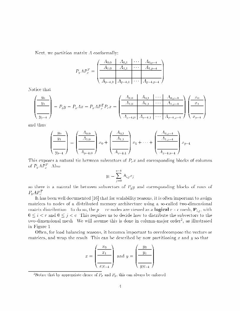
Next, we partition matrix A conformally:PyAP Tx = 0BBBB@ A0;0 A0;1 � � � A0;p�1A1;0 A1;1 � � � A1;p�1... ... ...Ap�1;0 Ap�1;1 � � � Ap�1;p�1 1CCCCANotice that0BBBB@ y0y1...yp�1 1CCCCA = Pyy = PyAx = PyAP Tx Pxx = 0BBBB@ A0;0 A0;1 � � � A0;p�1A1;0 A1;1 � � � A1;p�1... ... ...Ap�1;0 Ap�1;1 � � � Ap�1;p�1 1CCCCA0BBBB@ x0x1...xp�1 1CCCCAand thus 0BBBB@ y0y1...yp�1 1CCCCA = 0BBBB@ A0;0A1;0...Ap�1;0 1CCCCA x0 + 0BBBB@ A0;1A1;1...Ap�1;1 1CCCCA x1 + � � � + 0BBBB@ A0;p�1A1;p�1...Ap�1;p�1 1CCCCAxp�1This exposes a natural tie between subvectors of Pxx and corresponding blocks of columnsof PyAP Tx . Also yi = p�1Xj=0Ai;jxjso there is a natural tie between subvectors of Pyy and corresponding blocks of rows ofPyAP Tx .It has been well documented [16] that for scalability reasons, it is often important to assignmatrices to nodes of a distributed memory architecture using a so-called two-dimensionalmatrix distribution. To do so, the p = rc nodes are viewed as a logical r�c mesh, Pi;j , with0 � i < r and 0 � j < c. This requires us to decide how to distribute the subvectors to thetwo-dimensional mesh. We will assume this is done in column-major order2, as illustratedin Figure 1.Often, for load balancing reasons, it becomes important to overdecompose the vectors ormatrices, and wrap the result. This can be described by now partitioning x and y so thatx = 0BBBB@ x0x1...xN�1 1CCCCA and y = 0BBBB@ y0y1...yN�1 1CCCCA2Notice that by appropriate choice of Px and Py, this can always be enforced4

y
6y
9y
1y
2y
4y
3y
5y
y7
8y
0
10
2, 5
, 8,
11
y
11yR
ow in
dice
s of
blo
cks
of m
atri
x
0, 3
, 6,
91,
4,
7, 1
0
x
6x
9x
1x
2x
4x
3x
5x
x7
8x
10
0
x
9, 10, 11
11x
Column indices of blocks of matrix
0, 1, 2 3, 4, 5 6, 7, 8,
10,0
1,0
2,0
4,0
7,0
8,0
11,0
60
0,11
3,11
6,11
9,11
1,11
4,11
7,11
10,11
2,11
5,11
8,11
10,3
11,11
5,0
0,0
3,0
,9,0
0,1 0,2 0,3 0,4 0,5 0,6 0,7 0,8 0,9 0,10
3,1 3,2 3,4 3,5 3,6 3,7 3,8 3,9 3,10
6,1 6,2
9,1 9,2
4,1
7,1
10,1
2,1
5,1
8,1
11,1
1,2
4,2
7,2
5,2
11,2
4,3
7,3
11,3
2,3
5,3
8,3
11,3
6,3
9,3
6,4
9,4
1,4
7,4
10,4
2,4
8,4
11,4
6,5
1,5
4,5
7,5
10,5
2,5
8,5
11,5
9,6
1.6
4,6
7,6
10,6
5,6
8,6
11,6
9,7
1,7
4,7
10,7
2,7
5,7
8,7
11,7
6,8
9,8
1,8
4,8
7,8
2,8
5,8
11,8
6,9
1,9
4,9
7,9
2,9
5,9
8,9
11,9
6,10
9,10
1,10
4,10
2,10
5,10
8,10
11,10
1,3
9,5
10,8
8,2
5,4
2,6
6,7
1,1
2,2
3,3
4,4
5,5
6,6
7,7
8,8
9,9
10,1010,2
7,10
Figure 1: Inducing a matrix distribution from vector distributions. Top: The subvectors ofx and y are assigned to a logical 3 � 4 mesh of nodes. Top-left: By projecting the indicesof y to the left, we determing the distribution of the matrix row-blocks of A. Top-right: Byprojecting the indices of x to the top, we determing the distribution of the matrix column-blocks of A. The resulting distribution of the subblocks of A is given in the bottom picture,where the indices refer to the indices of the subblocks of A given in Eqn. (2).5
y21
,y ,...
10y
22,y ,...
11y
23,y ,...
3y
15,y ,...
4y
16,y ,...
5y
17,y ,...
,...
6y
18,y ,...
7y
19
9
,y
2,5,
8,11
,14,
...
,...
8y
20,y ,...
0y
12,y ,...
1y
13,y ,...
2y
14,y ,...
Row
indi
ces
of b
lock
s of
mat
rix
0,3,
6,9,
12,..
.1,
4,7,
10,1
3
x21
,x ,...
10x
22,x ,...
11x
23,x ,...
3x
15,x ,...
4x
16,x ,...
5x
17,x ,...
,...
6x
18,x ,...
7x
19,x
9
,...
0,1,2,12,13,...
8x
20,x ,...
0x
12,x ,...
1x
13,x ,...
2x
14,x ,...
3,4,5,15,16,... 6,7,8,18,19,... 9,10,11,21,22,...
Column indices of blocks of matrix
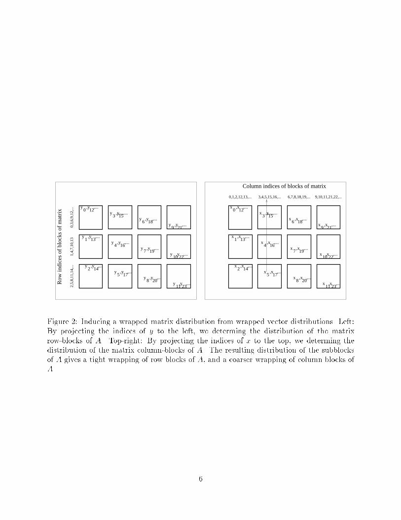
Figure 2: Inducing a wrapped matrix distribution from wrapped vector distributions. Left:By projecting the indices of y to the left, we determing the distribution of the matrixrow-blocks of A. Top-right: By projecting the indices of x to the top, we determing thedistribution of the matrix column-blocks of A. The resulting distribution of the subblocksof A gives a tight wrapping of row blocks of A, and a coarser wrapping of column blocks ofA.6

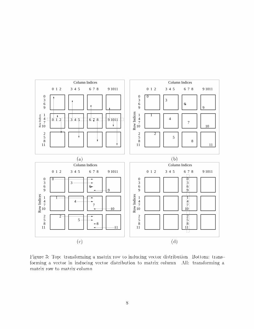
where N >> p. Partitioning A conformally yields the blocked matrixA = 0BBBB@ A0;0 A0;1 � � � A0;N�1A1;0 A1;1 � � � A1;N�1... ... ...AN�1;0 AN�1;1 AN�1;N�1 1CCCCA (2)A wrapped distribution can now be obtained by wrapping the blocks of x and y, whichinduces a wrapping in the distribution of A, as illustrated in Figure 2. Notice that in somesense, this second distribution is equivalent to the �rst, since the appropriate permutationsPx = Py will take one vector distribution to the other. However, exposing the wrappingexplicitly will become important for the library implementation.3 Impact of PBMD on library implementationIn this section, we will show how the existence of an inducing vector distribution allows usto parallelize the accepted basic building blocks for dense linear algebra libraries, the BasicLinear Algebra Subprograms (BLAS). We will do so, by �rst showing how the inducingvector distribution helps us organize necessary data movements, which we will subsequentlyshow allow us to conveniently parallelize matrix-vector multiplication and rank-1 updates.Next, we will argue how the operations performed by matrix-vectormultiplication and rank-1update are fundamental to the implementation of more complex BLAS such as matrix-matrixmultiplication.3.1 Vectors, matrix-rows, and -columnsWe start by showing how matrix distributions that are induced by vector distributions nat-urally permit redistribution of rows and columns of matrices to the inducing vector distri-bution, as well as redistribution of matrix rows to columns, and visa versa.Vector to matrix row, matrix row to vector: Consider a vector, x, distributed tonodes according to an inducing vector distribution for matrix A. Notice that the as-signment of blocks of columns of A is determined by a projection of the indices ofthe corresponding subvectors of the inducing vector distribution. Thus, transforminga vector x into a row of A is equivalent to projecting onto that matrix row, or, equiva-lently, gathering the subvectors of x within columns of nodes to the row of nodes thatholds the desired row of A. Naturally, redistributing a row of the matrix to a vectorreverses this process, requiring a scatter within columns of A, as illustrated in Fig. 3.7
0 1 2 3 4 5 6 7 8 9 10
0369
147
10
258
11
110 1 2 3 4 5
11
6
Column Indices
7 8 9 10
Row
Ind
ices
369
147
10
258
11
6
003
69
14
710
25
811
Row
Ind
ices
110 1 2 3 4 5 6 7 8 9 10
Column Indices
(a) (b)6
0
1
3
4
52
6
7
8
9
10
11
110 1 2 3 4 5 6 7 8 9 10
0369
147
10
258
11
Column Indices
Row
Ind
ices
369
147
10
258
11
0369
147
10
258
11
0
Row
Ind
ices
110 1 2 3 4 5 6 7 8 9 10
Column Indices
(c) (d)Figure 3: Top: transforming a matrix row to inducing vector distribution. Bottom: trans-forming a vector in inducing vector distribution to matrix column. All: transforming amatrix row to matrix column. 8

3 4 5 6 7 8 9 100 1 2 11
1
3
4
5
7
8
9
10
11
Column Indices
6
0
2
0 1 2 3 4 5 6 7 8 9 10
110 1 2 3 4 5 6 7 8 9 10
110 1 2 3 4 5
11
6 7 8 9 10
110 1 2 3 4 5 6 7 8 9 10
Column Indices
Figure 4: Spreading a vector in inducing vector distribution within columns of nodes.Vector to matrix column, matrix column to vector: The vector to matrix columnoperation is similar to the redistribution of a vector to a matrix row, except that thegather is performed within rows of nodes, as illustrated in Fig. 3. Again, the matrixcolumn to vector operation is reverses this process.Matrix row to matrix column, matrix column to matrix row: Redistributing amatrix row to become a matrix column, i.e. transposing a matrix row to become amatrix column, can be achieved by redistributing from matrix row to inducing vectordistribution, followed by a redistribution from vector distribution to matrix column,as illustrated in Fig. 3. Naturally, reversing this process takes a matrix column to amatrix row.3.2 Spreading vectors, matrix rows, and matrix columnsA related operation is the spreading of vectors, matrix rows, and matrix columns withinrows or columns of nodes. Given a vector, matrix row, or matrix column, these operationsresult in a copy of a row or column vector being owned by all rows of nodes or all columnsof nodes.Spreading a vector within rows (columns) of nodes: Notice that while gathering avector within rows (columns) to a speci�ed column (row) of nodes can be used to yielda column (row) vector. If we wish to have a copy of this column (row) vector within9
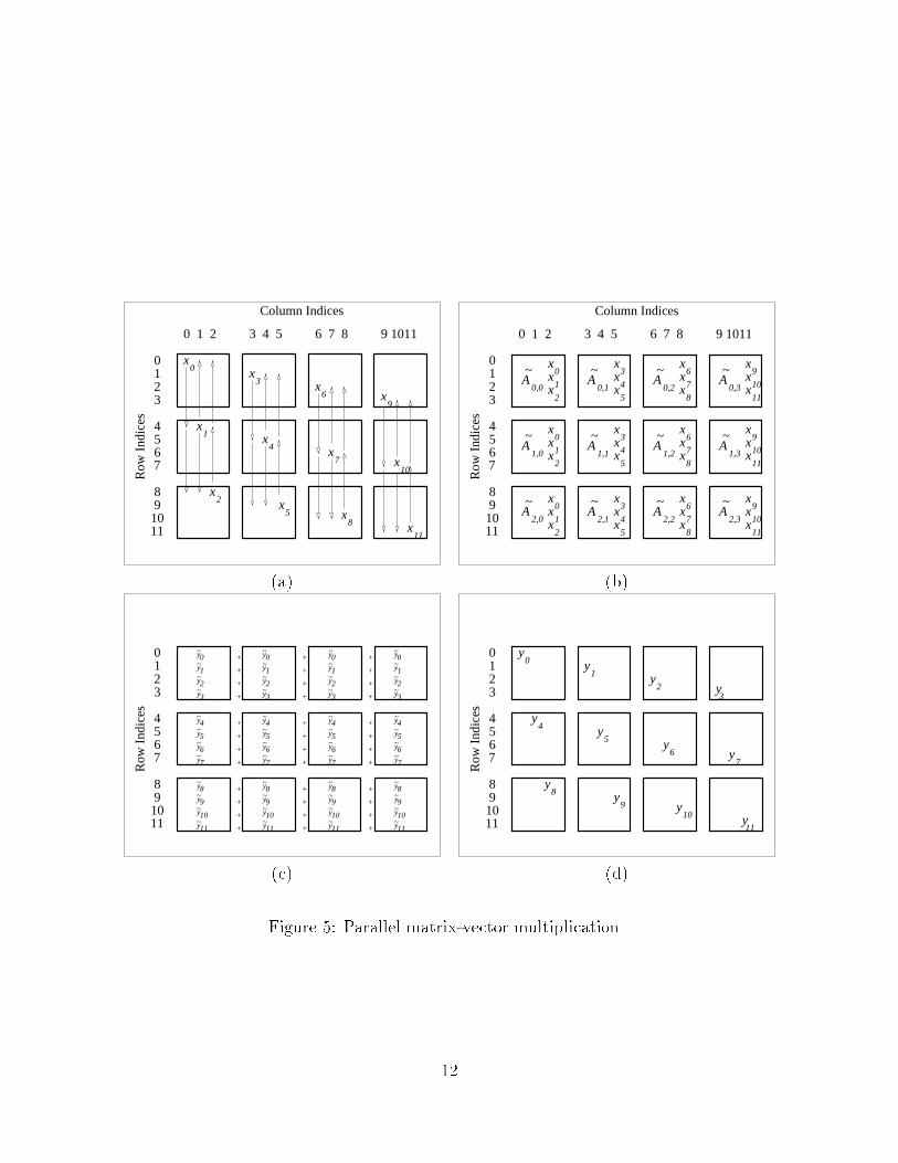
each column (row) of nodes, we need merely collect the vector within rows (columns)of nodes, as illustrated in Fig. 4.Spreading a matrix row (column) within columns (rows) of nodes: Given a matrixrow, we often require a copy of this matrix row to exist within each row of nodes, anoperation that we will call spreading a matrix row within columns of nodes. Oneapproach is to redistribute the matrix row like the inducing vector distribution, andspreading the resulting vector, requiring a scatter followed by a collect, both withincolumns. Since a scatter followed by a collect is equivalent to a broadcast, broadcast-ing the pieces of the matrix row within columns can be viewed as a shortcut. Similarly,spreading a matrix column within rows of nodes can be accomplished by broadcastingthe appropriate pieces of the matrix column within rows of nodes.Spreading a matrix row (column) within rows (columns) of nodes: Spreading amatrix row within rows of nodes is logically equivalent to redistributing the matrixrow like the inducing vector distribution, followed by a spreading of the vector witinrow of nodes. Notice that this requires a scatter within columns of nodes, followed bya collect within rows of nodes. Spreading a matrix column within columns of nodescan be accomplished similarly.3.3 DiscussionIt is important to note that the above observations expose an extremely systematic approachto the required data movement. It naturally exposes the inducing vector distribution as anintermediate step through which redistribution of rows and columns of matrices can beimplemented in a building-block approach.4 Implementation of basic matrix-vector operationsWe now have the tools for the implementation of the basic matrix-vector operations. We willconcentrate on the most widely used: the matrix-vector multiplication and rank-1 update.4.1 Matrix-vector multiplicationThe basic operation to be performed is given by Ax = y.Ax ! y, x and y distributed like vectors: For this case, assume that x and y areidentically distributed according to the inducing vector distribution that induced thedistribution of matrix A. Notice that by spreading vector x within columns, weduplicate all necessary elements of x so that local matrix vector multiplication can10

commense on each node. After this, a summation within rows of nodes of the localpartial results yields the desired vector y. However, since only a portion of vectory needs to be known to each node, a distributed summation (MPI Reduce scatter)within rows of nodes su�ces. This process is illustrated in Fig. 5.Ax! y, matrix row x and matrix column y: Again, we wish to perform Ax = y, butthis time we assume that x and y are a row and column of a matrix, respectively, wherethe distribution of that matrix is induced by the same inducing vector distribution asthat of matrixA. Notice that by spreadingmatrix row x within columns, we duplicateall necessary elements of x so that local matrix vector multiplication can commense oneach node. After this, a summation within rows of nodes of the local partial resultsyields the desired vector y. Since y is a column, existing on only one column of nodes,a summation to one node (MPI Reduce) within each row of nodes can be utilized.Ax! y, matrix column x and matrix row y: Now we assume that x and y are a columnand row of a matrix, respectively, where the distribution of that matrix is induced bythe same inducing vector distribution as that of matrix A. Notice that by spreadingmatrix column x within rows of nodes, we duplicate all necessary elements of x sothat local matrix vector multiplication can commense on each node. After this, asummation within rows of nodes (MPI Reduce scatter) must occur, leaving the resultin inducing vector distribution. The �nal operation is to redistribute the result to therow of the target matrix.4.2 Rank-1 updateThe basic operation to be performed is given by A = A+ yxT .A = A+ yxT , x and y distributed like vectors: For this case, assume that x and y areidentically distributed according to the inducing vector distribution that induced thedistribution of matrix A. Notice that by spreading vectors x and y within columnsand rows of nodes, respectively, we duplicate all necessary elements of x and y so thatlocal rank-1 updates can commense on each node.A = A+yxT , other cases: The case where x and y start as row or column of a matrix canbe derived similar to the special cases of matrix-vector multiplication. For simplicity,we will concentrate on the square matrix case, but the techniques generalize.5 Implementation of basic matrix-matrix operationsWe now show how the parallel matrix-vector multiplication and rank-1 update can be usedto implement matrix-matrix multiplication, and other level-3 BLAS. In all our explanations,11
3 4 5 6 7 8 9 100 1 2
x
x
x
x
x
x
x
11
x
x
x
x
x
0
1
2
3
4
5
6
7
8
10Row
Ind
ices
0123
4567
891011
Column Indices
9
11
0 1 2 3 4 5 6 7 8 9 10
x0x
x
xxx
xxx
xxx1
2
3
4
5
6
7
8
9
10
11
x0x
x
xxx
xxx
xxx1
2
3
4
5
6
7
8
9
10
11
x0x
x1
2
11
Row
Ind
ices
0123
4567
891011
Column Indices
A~
A~
A~
A~
0,0
A~
1,0A~
A~
A~
A~
2,0A~
A~
A~
1,1
2,1
1,2
0,1 0,2
2,2
0,3
1,3
2,3
xxx
xxx
xxx
3
4
5
6
7
8
9
10
11
(a) (b)~y~y~y~0
1
2
3 y~y~y~y~0
1
2
3 y~y~y~y~0
1
2
3y~y~y~y~0
1
2
3 +
+
+
+
+
+
+
+
+
+
+
+
+
+
+
+
+
+
+
+
+
+
+
+
+
+
+
+
+
+
y
+
+
+
+
+
+
y~y~y~y~
5
6
7
4
y~y~y~y~8
9
10
11 y~y~y~y~8
9
10
11
y~y~y~y~
5
6
7
4
y~y~y~y~
5
6
7
4
y~y~y~y~8
9
10
11y~y~y~y~8
9
10
11
y~y~y~y~
5
6
7
4
Row
Ind
ices
0123
4567
891011
0
1
23
4
5
67
8
910
11
yy
yy
yy
yy
yy
yy
Row
Ind
ices
0123
4567
891011(c) (d)Figure 5: Parallel matrix-vector multiplication.12

we will use the following partitionings:X = � x0 x1 � � � xn�1 � (3)with X 2 fA;B;Cg and x 2 fa; b; cg where xj represents the jth column of X. Also,X = 0BBBB@ xT0xT1...xTn�1 1CCCCA (4)where xTi represents the ith row of matrix X.5.1 Matrix-matrix multiplicationC = AB: Parallelizing C = AB becomes straight-forward when one observes thatC = AB = a0bT0 + a1bT1 + � � �+ an�1bTn�1Thus the parallelization of this operation can proceed as a sequence of rank-1 updates,with the vectors y and x equal to the appropriate column and row of matrices A andB, respectively.C = ABT : For this case, we note thatcj = AbTj ; j = 0; : : : ; n� 1This time, the parallelization of the operation can proceed as a sequence of matrix-vector multiplications, with the vectors y and x equal to the appropriate column androw of matrices C and B, respectively.C = ATB: Notice that C = ATB is equivalent to computing CT = BTA, and thus thecomputation can proceed by computingci = BTai; i = 0; : : : ; n� 1The matrix-vector multiplication schemes described earlier can be easily adjusted toaccomodate for this special case.C = ATBT : On the surface, this operation appears quite straight-forward:C = ATBT = a0bT0 + a1bT1 + � � �+ an�1bTn�113

Thus the parallelization of this operation can proceed as a sequence of rank-1 updates,with the vectors y and x equal to the appropriate row and column of matrices Aand B, respectively. However, notice that the required spreading of vectors is quitedi�erent, as described in Section 3.2. It should be noted that without the observationsmade about spreading matrix rows and columns by �rst redistributing like the inducingvector distribution, this operation is by no means trivial when the mesh of nodes isnonsquare.5.2 Attaining better performanceThe above approach, while simple, will not yield high performance, since all local operationsare performed using level-2 BLAS. Better (near peak) performance can be attained by re-placing matrix-vector multiplication by matrix-panel-of-vectors multiplication, and rank-1updates by rank-k updates. The algorithms outlined above can be easily altered to accomo-date this.5.3 Other level 3 BLASIn [4], we describe how all level 3 BLAS can be implemented using variations of the abovescheme, attaining within 10-20% of peak performance on the Intel Paragon.6 A Simple LibraryAs part of the PLAPACK project at the University of Texas at Austin, we have set out toinvestigate the implications of the above mentioned observations. In order to do so, we haveimplemented a prototype library, the SL Library, that incorporates the techniques.In addition to layering the library using these techniques, we have adopted an \objectbased" approach to programming. This approach has already popularized for high perfor-mance parallel computing by libraries like the Toolbox being developed at Mississippi StateUniversity [1], the PETSc library at Argonne National Laboratory [15] and the Message-Passing Interface [14].6.1 ScopeThe goal of our scaled down e�ort is to demonstrate how the observed techniques simplifythe implementation of linear algebra libraries by providing a systematic (building-block)approach. We emphasize here that it is the systematic nature of the techniques that is ofgreat importance to comprehensive library development. While we hint at the fact thatstarting with vector distributions can yield any arbitrary cartesian matrix distribution, we14
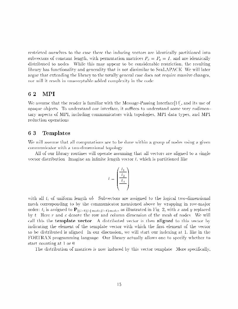
restricted ourselves to the case there the inducing vectors are identically partitioned intosubvectors of constant length, with permutation matrices Px = Py = I, and are identicallydistributed to nodes. While this may appear to be considerable restriction, the resultinglibrary has functionality and generality that is not dissimilar to ScaLAPACK. We will laterargue that extending the library to the totally general case does not require massive changes,nor will it result in unacceptable added complexity in the code.6.2 MPIWe assume that the reader is familiar with the Message-Passing Interface[14], and its use ofopaque objects. To understand our interface, it su�ces to understand some very rudimen-tary aspects of MPI, including communicators with topologies, MPI data types, and MPIreduction operations.6.3 TemplatesWe will assume that all computations are to be done within a group of nodes using a givencommunicator with a two-dimensional topology.All of our library routines will operate assuming that all vectors are aligned to a singlevector distribution. Imagine an in�nite length vector t, which is partitioned liket = 0BBBB@ t1t2t3... 1CCCCAwith all ti of uniform length nb. Subvectors are assigned to the logical two-dimensionalmesh corresponding to by the communicator mentioned above by wrapping in row-majororder: ti is assigned to Pb(i�1)=ccmodr;(i�1)mod c, as illustrated in Fig. 2, with x and y replacedby t. Here r and c denote the row and column dimension of the mesh of nodes. We willcall this the template vector. A distributed vector is then aligned to this vector byindicating the element of the template vector with which the �rst element of the vectorto be distributed is aligned. In our discussion, we will start our indexing at 1, like in theFORTRAN programming language. Our library actually allows one to specify whether tostart counting at 1 or 0.The distribution of matrices is now induced by this vector template. More speci�cally,15

let T be an in�nite matrix, partitioned likeT = 0BBBB@ T1;1 T1;2 T1;3 � � �T2;1 T2;2 T2;3 � � �T3;1 T3;2 T3;3 � � �... ... ... 1CCCCAwhere Ti;j are nb � nb submatrices. Then this template matrix is distributed to nodesas induced by the template vector, t, which is the inducing vector distribution as describedearlier in this paper. A given matrix to be distributed is now aligned to this template byindicating the element of T with which the (1; 1) element of the matrix to be distributed isaligned.Initializing the template is accomplished with a call to the routineint SL_Temp_create( MPI_Comm comm,int nb,int zero_or_oneSL_Template *template )where comm passes the MPI communicator with two-dimensional topology, and nb equals theblocking size for the vector template. The value in zero or one speci�es what index to givethe �rst element in a matrix. A value of 1 means that matrix and vector indicies start at 1.A value of 0 means that matrix and vector indicies start at zero. The result of this operationis an opaque object, a data structure that encodes the information about the mapping ofvectors and matrices to the node mesh.Rather than accessing the data structure directly, the library provides a large number ofinquiry routines, which can be used to query information about the mesh of nodes and thedistribution of the template.6.4 Linear Algebra ObjectsVector and matrix, in general Linear Algebra Objects (LAObj), distributution is nowgiven with respect to the above described distribution template. Again, we use opaqueobjects to encode all information, which includes the template, and how the given object isaligned to the template. Thus, in order to create a vector object, which includes creation ofthe data structure that holds the information and space for the local data to be stored, acall to the following routine is made:int SL_Vector_create (MPI_Datatype datatype,int global_length,SL_Template template,int global_align,SL_LAObj *new_vector)16
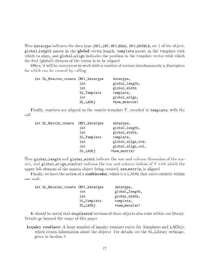
Here datatype indicates the data type (MPI INT, MPI REAL, MPI DOUBLE, etc.) of the object,global length passes in the global vector length, template passes in the template withwhich to align, and global align indicates the position in the template vector with whichthe �rst (global) element of the vector is to be aligned.Often, it will be convenient to work with a number of vectors simultaneously, a discriptionfor which can be created by callingint SL_Mvector_create (MPI_Datatype datatype,int global_length,int global_widthSL_Template template,int global_align,SL_LAObj *new_mvector)Finally, matrices are aligned to the matrix template T , encoded in template, with thecall int SL_Matrix_create (MPI_Datatype datatype,int global_length,int global_width,SL_Template template,int global_align_row,int global_align_col,SL_LAObj *new_matrix)Here global length and global width indicate the row and column dimension of the ma-trix, and global align row/col indicate the row and column indices of T with which theupper left element of the matrix object being created, new matrix, is aligned.Finally, we have the notion of amultiscalar, which is a LAObj that exists entirely withinone node.int SL_Mscalar_create (MPI_Datatype datatype,int global_length,int global_width,SL_Template template,SL_LAObj *new_mscalar)It should be noted that duplicated versions of these objects also exist within our library.Details go beyond the scope of this paper.Inquiry routines: A large number of inquiry routines exists for Templates and LAObjs,which return information about the objects. For details, see the SL Library webpage,given in Section 8. 17
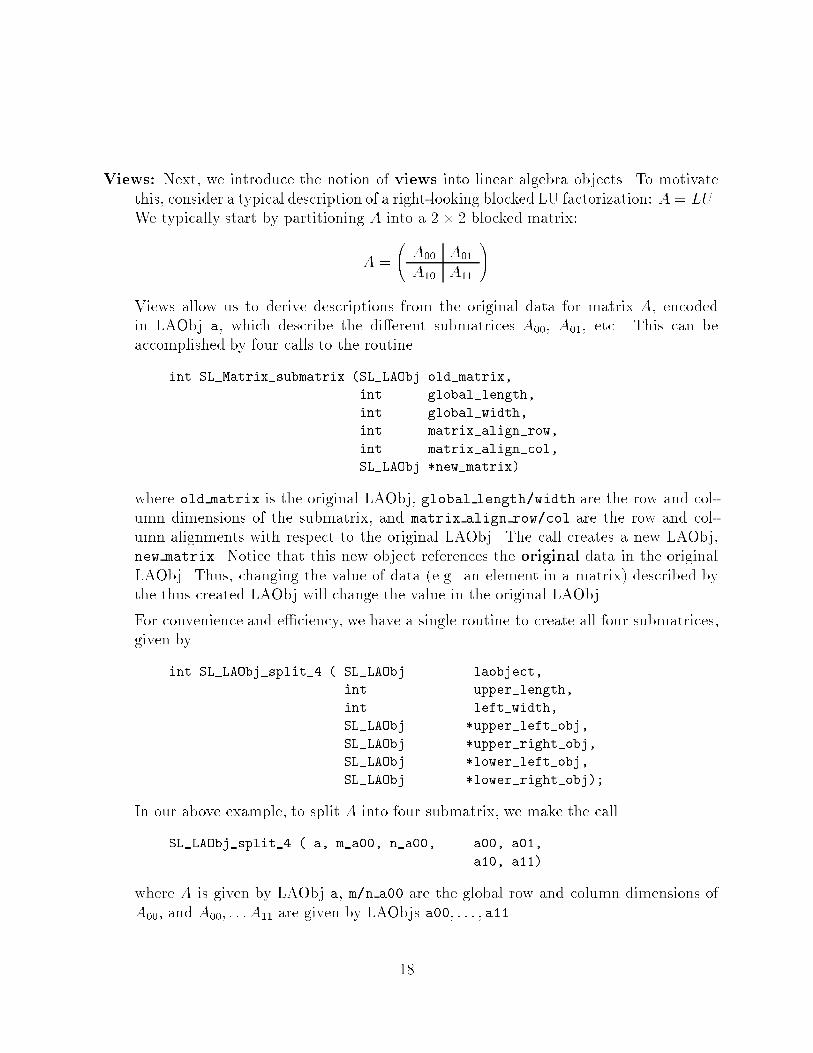
Views: Next, we introduce the notion of views into linear algebra objects. To motivatethis, consider a typical description of a right-looking blocked LU factorization: A = LU .We typically start by partitioning A into a 2 � 2 blocked matrix:A = A00 A01A10 A11 !Views allow us to derive descriptions from the original data for matrix A, encodedin LAObj a, which describe the di�erent submatrices A00, A01, etc. This can beaccomplished by four calls to the routineint SL_Matrix_submatrix (SL_LAObj old_matrix,int global_length,int global_width,int matrix_align_row,int matrix_align_col,SL_LAObj *new_matrix)where old matrix is the original LAObj, global length/width are the row and col-umn dimensions of the submatrix, and matrix align row/col are the row and col-umn alignments with respect to the original LAObj. The call creates a new LAObj,new matrix. Notice that this new object references the original data in the originalLAObj. Thus, changing the value of data (e.g. an element in a matrix) described bythe thus created LAObj will change the value in the original LAObj.For convenience and e�ciency, we have a single routine to create all four submatrices,given byint SL_LAObj_split_4 ( SL_LAObj laobject,int upper_length,int left_width,SL_LAObj *upper_left_obj,SL_LAObj *upper_right_obj,SL_LAObj *lower_left_obj,SL_LAObj *lower_right_obj);In our above example, to split A into four submatrix, we make the callSL_LAObj_split_4 ( a, m_a00, n_a00, a00, a01,a10, a11)where A is given by LAObj a, m/n a00 are the global row and column dimensions ofA00, and A00; : : : A11 are given by LAObjs a00; : : : ; a11.18

6.5 Parallel Basic Linear Algebra SubprogramsGiven that all information about vectors and matrices is now encoded in LAObjs, the callingsequences for routines like the Basic Linear Algebra Subprograms now becomes relativelystraight forward. We give examples for one from each of the level 1, 2, and 3 BLAS.Level 1 BLAS: The level 1 BLAS include operations like the gaxpy, which adds a multipleof a vector to a vector: y �x+ y. The double precision sequential call isvoid daxpy (int *n, double *alpha, double *x, int *incx,double *y, int *incy )The SL Library call becomesint SL_Axpy (SL_LAOBJ alpha,SL_LAObj aobj_x,SL_LAObj aobj_y)Naturally, we no longer need to restrict ourselves to requiring x and y to be onlyvectors. The call will also work for multiscalars, multivectors and matrices.Level 2 BLAS: The level 2 BLAS include operations like the ggemv, which adds a multipleof a matrix-vector product to a vector: y �Ax+ y. The SL Library call is given byint SL_Gemv (int trans,SL_LAObj alpha,SL_LAObj a,SL_LAObj x,SL_LAObj beta,SL_LAObj y)Level 3 BLAS: The level 3 BLAS include operations like the ggemm, which adds a multipleof a matrix-matrix product to a matrix: C �AB+�C. The SL Library call is givenby int SL_Gemm (int transa,int transb,SL_LAObj alpha,SL_LAObj a,SL_LAObj b,SL_LAObj beta,SL_LAObj c)19

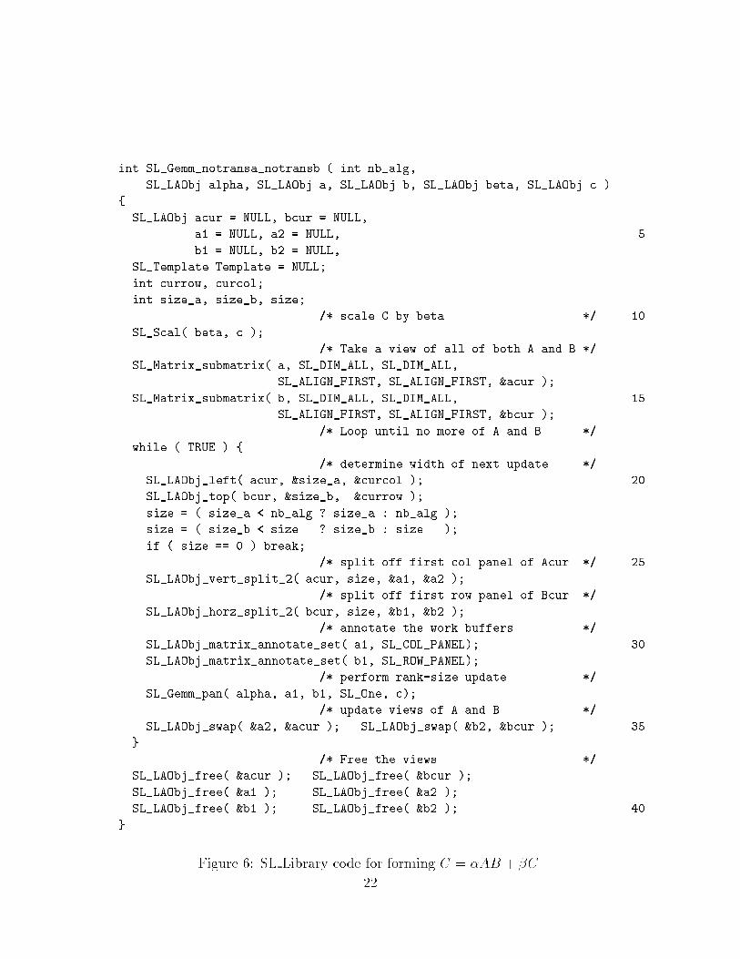
6.6 Communication in the libraryOur library has only two communication routines; the copy routine, which copies from oneLAObj to another, and the reduce operator, which consolidates contributions from di�erentLAObjs.int SL_Copy (SL_LAObj aobj_from,SL_LAObj aobj_to)int SL_Reduce (SL_LAObj aobj_from,MPI_Op op,SL_LAObj aobj_to)6.7 Sample implementation: matrix-matrix multiplicationAs described above, parallel matrix-matrix multiplication can be implemented as a sequenceof rank-k updates. In this section, we again describe that process, except this time as arecursive algorithm.Algorithm: Let C = �AB + �C. PartitioningA = � A1 A2 � and B = B1B2 !we see that if we start by overwriting C �C, we subsequently must form C =C + �A1B1 + �A2B2. The algorithm thus becomes1. C �C2. Repeat until A and B are empty(a) A = � A1 A2 � and B = B1B2 !(b) C �A1B2(c) A = A2 and B = B2Here the width of A1 and height of B1 is chosen so that both conform, and both thesepanels of matrices exist in one column of nodes and one row of nodes, respectively.Code: The code, as written in the SL Library is now given in Fig. 6. Given the abovealgorithm, we believe the code to be largely self-explanatory. It is meant to give animpression of what can be done with the infrastructure we have put together as partof the SL Library.The only line of code that does require some detailed explanation is line 33:20
SL_Gemm_pan( alpha, a1, b1, SL_One, c);This call performs a rank-size update to matrix C. It is in this routine that all datamovements, and calls to local BLAS on each node, are hidden.Performance: The performance of the above matrix-matrix routine on an Intel Paragonsystem and an IBM SP-2 is given in Figs. 7 and 8. It should be noted that thepeak performance on the Intel Paragon for matrix-matrix multiplication is around 46MFLOPS on a single node. On a single node of our SP-2, the matrix-matrix multiplyBLAS routine attains around 240 MFLOPS. Thus, our parallel library routine attainsvery good performance, once the matrices are reasonably large. While our preliminaryperformance numbers are only for a small number of nodes, the techniques are perfectlyscalable and thus very high performance can be expected, even for very large numbersof nodes. We justify this statement in [4] and other papers.While the given data is by no means conclusive, we should note that much more extensivedata for the techniques is given in a previous paper of ours [4], where we show how indeed alllevel 3 BLAS can be implemented in this fashion. In that paper, we also show the techniquesto be scalable. Thus, the presented data should be interpreted to show that the infrastructurewe have created, even without tuning, does not create unreasonable performance degradation.Ideally, we would have included a performance comparison with other available parallellinear algebra libraries, like ScaLAPACK. However, ScaLAPACK is due for a release of amajor revision, thus no reasonable data could be collected at this time for that package. Weintend to include such a comparison in the �nal document.7 ConclusionAs mentioned, the SL Library is a prototype library, which is meant to illustrate the bene�tsof the described approaches. Design of this library, and its extention, PLAPACK, was startedin Fall 1995. Coding commensed in mid-March. At this time, the infrastructure is essentiallycomplete, and a few of the parallel BLAS have been implemented. A large number ofroutines, including LU/Cholesky/QR factorization, reduction to banded or condensed formand Jacobi's method for dense eigenproblems, have been designed and implemented, but notyet debugged. Essentially all of these implementations exploit some aspect of the library thatallows for new and presumably higher performance algorithms. By the end of summer 1996,our limited implementation library will have functionality and scope that will be essentiallyequivalent to that of the more established ScaLAPACK library. It is important to note thatthis will be attained in approximately 5,000 lines of code, which represents a two order-of-magnitude reduction in code. 21
int SL_Gemm_notransa_notransb ( int nb_alg,SL_LAObj alpha, SL_LAObj a, SL_LAObj b, SL_LAObj beta, SL_LAObj c ){ SL_LAObj acur = NULL, bcur = NULL,a1 = NULL, a2 = NULL, 5b1 = NULL, b2 = NULL,SL_Template Template = NULL;int currow, curcol;int size_a, size_b, size; /* scale C by beta */ 10SL_Scal( beta, c ); /* Take a view of all of both A and B */SL_Matrix_submatrix( a, SL_DIM_ALL, SL_DIM_ALL,SL_ALIGN_FIRST, SL_ALIGN_FIRST, &acur );SL_Matrix_submatrix( b, SL_DIM_ALL, SL_DIM_ALL, 15SL_ALIGN_FIRST, SL_ALIGN_FIRST, &bcur );/* Loop until no more of A and B */while ( TRUE ) { /* determine width of next update */SL_LAObj_left( acur, &size_a, &curcol ); 20SL_LAObj_top( bcur, &size_b, &currow );size = ( size_a < nb_alg ? size_a : nb_alg );size = ( size_b < size ? size_b : size );if ( size == 0 ) break; /* split off first col panel of Acur */ 25SL_LAObj_vert_split_2( acur, size, &a1, &a2 );/* split off first row panel of Bcur */SL_LAObj_horz_split_2( bcur, size, &b1, &b2 );/* annotate the work buffers */SL_LAObj_matrix_annotate_set( a1, SL_COL_PANEL); 30SL_LAObj_matrix_annotate_set( b1, SL_ROW_PANEL);/* perform rank-size update */SL_Gemm_pan( alpha, a1, b1, SL_One, c);/* update views of A and B */SL_LAObj_swap( &a2, &acur ); SL_LAObj_swap( &b2, &bcur ); 35} /* Free the views */SL_LAObj_free( &acur ); SL_LAObj_free( &bcur );SL_LAObj_free( &a1 ); SL_LAObj_free( &a2 );SL_LAObj_free( &b1 ); SL_LAObj_free( &b2 ); 40} Figure 6: SL Library code for forming C = �AB + �C.22
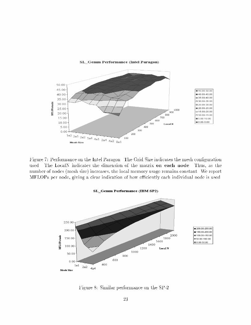
Figure 7: Performance on the Intel Paragon. The Grid Size indicates the mesh con�gurationused. The LocalN indicates the dimension of the matrix on each node. Thus, as thenumber of nodes (mesh size) increases, the local memory usage remains constant. We reportMFLOPs per node, giving a clear indication of how e�ciently each individual node is used.Figure 8: Similar performance on the SP-2.23

In [1] and other references, it is pointed out that parallel linear algebra libraries shouldallow for highly irregular distributions. In [5, 10], we show how all two-dimensional cartesianmatrix distributions can be viewed as being induced by vector distributions and how thisallows for even more exible libraries. It is this ability to work with highly general andirregular blockings and distributions of matrices that will ultimately allow us to implementmore general libraries than previously possible, as part of the full PLAPACK library. Alsoin the planning are out-of-core extensions [17].It is often questioned whether the emphasis on dense linear algebra is misplaced in the�rst place [9]. It is our position that the future of parallel dense linear algebra is in asupport role for parallel sparse linear solvers, to solve dense subproblems that are part ofvery large sparse problems (e.g. exploited by parallel supernodal methods [21, 22]). It isthus important that the approach to distributing and manipulating the dense matrices isconformal with how they naturally occur as part of the sparse problem. Since our matrixdistribution starts with the vector, we believe the described approach meets this criteria.For details, see [10]. Ultimately, we will build on the presented infrastructure, including thesupport for parallel dense linear algebra, and incorporate sparse iterative and sparse directmethods into PLAPACK.8 Further informationThis paper is meant to be a pointer to the web sites for the SL Library and PLAPACKproject:http://www.cs.utexas.edu/users/rvdg/SL library/library.htmlhttp://www.cs.utexas.edu/users/rvdg/paper/plapack.htmlReferences[1] Purushotham Bangalore, Anthony Skjellum, Chuck Baldwin, and Steven G. Smith,\Dense and Iterative Concurrent Linear Algebra in the Multicomputer Toolbox," inProceedings of the Scalable Parallel Libraries Conference (SPLC '93), pages132-141, Oct. 1993.[2] J. Choi, J. J. Dongarra, R. Pozo, and D. W. Walker, \Scalapack: A Scalable LinearAlgebra Library for Distributed Memory Concurrent Computers, Proceedings of theFourth Symposium on the Frontiers of Massively Parallel Computation. IEEEComput. Soc. Press, 1992, pp. 120-127.[3] J. Choi, J. Dongarra, and D. Walker, \The Design of a Parallel Dense Linear AlgebraSoftware Library: Reduction to Hessenberg, Tridiagonal, and Bidiagonal Form," UT,24

CS-95-275, February 1995.Related technical reports: http://www.netlib.org/lapack/lawns[4] Almadena Chtchelkanova, John Gunnels, Greg Morrow, James Overfelt, Robert A. vande Geijn, "Parallel Implementation of BLAS: General Techniques for Level 3 BLAS,"Concurrency: Practice and Experience to appear.http://www.cs.utexas.edu/users/rvdg/abstracts/sB BLAS.html[5] Almadena Chtchelkanova, Carter Edwards, John Gunnels, Greg Morrow, James Over-felt, Robert A. van de Geijn, "Comprehensive Approach to Parallel Linear Algebra Li-braries," unpublished manuscript prepared for the BLAS Technical Workshop, KnoxvillTennessee, Nov. 13-14, 1995http://www.cs.utexas.edu/users/rvdg/papers/plapack.html[6] Tom Cwik, Robert van de Geijn, and Jean Patterson, \The Application of ParallelComputation to Integral Equation Models of Electromagnetic Scattering," Journal ofthe Optical Society of America A , Vol. 11, No. 4, pp. 1538-1545, April 1994.[7] J. J. Dongarra, J. Du Croz, S. Hammarling, and I. Du�, \A Set of Level 3 Basic LinearAlgebra Subprograms," TOMS, Vol. 16, No. 1, pp. 1{17, 1990.[8] Jack Dongarra, Robert van de Geijn, and David Walker, \Scalability Issues A�ectingthe Design of a Dense Linear Algebra Library," Special Issue on Scalability of ParallelAlgorithms, Journal of Parallel and Distributed Computing, Vol. 22, No. 3, Sept.1994.Related technical reports: http://www.netlib.org/lapack/lawns[9] A. Edelman, \Large Dense Numerical Linear Algebra in 1993: The Parallel ComputingIn uence". Journal of Supercomputing Applications. 7 (1993), pp. 113{128.[10] C. Edwards, P. Geng, A. Patra, and R. van de Geijn, "Parallel Matrix Decompositions:have we been doing it all wrong?" TR-95-39, Department of Computer Sciences, Uni-versity of Texas, Oct. 1995.http://www.cs.utexas.edu/users/rvdg/abstracts/PBMD.html[11] G. Fox, et al., Solving Problems on Concurrent Processors: Volume 1, PrenticeHall, Englewood Cli�s, NJ, 1988.[12] Po Geng, J. Tinsley Oden, Robert van de Geijn, \Massively Parallel Computation forAcoustical Scattering Problems using Boundary ElementMethods," Journal of Soundand Vibration, 191 (1), pp. 145-165, 1996.25

[13] Golub, G., Van Loan, C., F., Matrix Computations, 2nd Ed., 1989, The John Hop-kins University Press.[14] W. Gropp, E. Lusk, and A. Skjellum, Using MPI, MPI Press, 1994.[15] W. Gropp and B. Smith, \The design of data-structure-neutral libraries for the iterativesolution of sparse linear systems," Scienti�c Programming, to appear.http://www.mcs.anl.gov/petsc/petsc.html[16] B. A. Hendrickson and D. E. Womble, \The Torus-Wrap Mapping for Dense MatrixCalculations on Massively Parallel Computers," SIAM J. Sci. Comput., check issuenumber[17] Ken Klimkowski and Robert van de Geijn, \Anatomy of an out-of-core dense linearsolver", Vol III - Algorithms and Applications Proceedings of the 1995 Inter-national Conference on Parallel Processing , pp. 29{33, 1995.[18] J. G. Lewis and R. A. van de Geijn, \Implementing Matrix-Vector Multiplication andConjugate Gradient Algorithms on Distributed Memory Multicomputers," Supercom-puting '93.[19] J. G. Lewis, D. G. Payne, and R. A. van de Geijn, \Matrix-Vector Multiplication andConjugate Gradient Algorithms on Distributed Memory Computers," Scalable HighPerformance Computing Conference 1994.[20] W. Lichtenstein and S. L. Johnsson, "Block-Cyclic Dense Linear Algebra", HarvardUniversity, Center for Research in Computing Technology, TR-04-92, Jan., 1992.[21] E. Rothberg and R. Schreiber, \Improved load distribution in parallel sparse Choleskyfactorization." in Proceedings of Supercomputing 94, pp. 783{792.[22] E. Rothberg and R. Schreiber, \E�cient parallel sparse Cholesky factorization," inProceedings of the Seventh SIAM Conference on Parallel Processing forScienti�c Computing (R. Schreiber, et al. eds.), SIAM, 1994, pp. 407{412.[23] Robert van de Geijn and Jerrell Watts, \SUMMA: Scalable Universal Matrix Multipli-cation Algorithm," Concurrency: Practice and Experience, to appear.26