18-819F: Introduction to Quantum Computing 47-779/47-785: Quantum Integer Programming

& Quantum Machine Learning

Review of Linear Algebra II

Lecture 02

2021.09.07.

• Dirac notation for complex linear algebra

– State vectors

– Linear operators – matrices

– Hermitian operators

– Unitary operators

– Projection operators and measurement

• Tensors

– Basis vectors for tensor product space

– Composite quantum systems

– Conception of tensor products as quantum entanglement

2

Agenda

Dirac Notation for Linear Algebra • We previously defined the inner (dot) product of two vectors 𝑢 and 𝑣 as

𝑢. 𝑣 = (𝑢, 𝑣),

where it was understood that 𝑢 is a row vector, which is better written as the transpose, 𝑢𝑇.

• This bracket notation was specialized by P.A.M Dirac, using angle brackets, to

𝑢. 𝑣 = 𝑢𝑇 . 𝑣 =< 𝑢| 𝑣 > = < 𝑢 𝑣 >;

• An ordinary row vector is now defined as: < 𝑢| = 𝑢1 𝑢2 … 𝑢𝑛 , where < | is the

“bra” and an ordinary column vector is |𝑣 > =

𝑣1𝑣2⋮𝑣𝑛

, where | > is the “ket” so that the

inner (dot) product is formed by the “bra-ket” < 𝑢|𝑣 >;

• The “bra” implicitly tells us to take the complex conjugate and the transpose of 𝑢.

3

Dirac Notation for Linear Algebra

• Having defined the notation, one can now use it to write most of ordinary vector and

matrix algebra;

• The outer product of two vectors, which we previously wrote as

𝑢𝑣𝑇 =

𝑢1𝑢2⋮𝑢𝑛

𝑣1 𝑣2 … 𝑣𝑛 =

𝑢1𝑣1 … 𝑢1𝑣𝑛⋮ … ⋮

𝑢𝑛𝑣1 … 𝑢𝑛𝑣𝑛Eqn. (3.1), is a matrix that can be

written succinctly as 𝑢𝑣𝑇 = |𝑢 >< 𝑣| (we prove this later) Eqn. (3.2);

• The outer product is often called a dyad and is a linear operator, i.e., a matrix.

4

• In 3D linear algebra, we said we can write a vector റ𝑣 as a linear combination of the basis

vectors Ƹ𝑒1, Ƹ𝑒2, Ƹ𝑒3, where 𝑣1, 𝑣2, 𝑣3 are the scaling coefficients

ቑ

റ𝑣 = 𝑣1 Ƹ𝑒1 + 𝑣2 Ƹ𝑒2 + 𝑣3 Ƹ𝑒3റ𝑣 = Ƹ𝑒1 Ƹ𝑒1

𝑇 . റ𝑣 + Ƹ𝑒2 𝑒2𝑇 . റ𝑣

റ𝑣 = Ƹ𝑒1 Ƹ𝑒1𝑇 + Ƹ𝑒2 Ƹ𝑒2

𝑇 + Ƹ𝑒3 Ƹ𝑒3𝑇 റ𝑣

+ Ƹ𝑒3 𝑒3𝑇 . റ𝑣

• From the 2nd equation above we have: 𝑣1 = Ƹ𝑒1𝑇 . റ𝑣 , 𝑣2 = Ƹ𝑒2

𝑇 . റ𝑣, 𝑣3 = 𝑒3𝑇 . റ𝑣;

• From the 3rd equation above we have 1 = Ƹ𝑒1 Ƹ𝑒1𝑇 + Ƹ𝑒2 Ƹ𝑒2

𝑇 + Ƹ𝑒3 Ƹ𝑒3𝑇 = σ𝑖=1

3 Ƹ𝑒𝑖 Ƹ𝑒𝑖𝑇;

• So σ𝑖=13 𝑒𝑖𝑒𝑖

𝑇 = 1 is the closure (completeness) relationship for the 3D vector space.

5

Dyad in 3D Vector Space

• In Hilbert space, a state vector |𝑣 > can be written as a linear combination of the basis

vectors |1 >, |2 >,… |𝑛 > with complex coefficients 𝑐1, 𝑐2, … 𝑐𝑛

ቑ

|𝑣 > = 𝑐1 1 > +𝑐2 2 > +⋯+ 𝑐𝑛|𝑛 >

|𝑣 > = |1 > < 1|𝑣 > + |2 > < 2 𝑣 > +⋯+ |𝑛 > (< 𝑛|𝑣 >

|𝑣 > = 1 >< 1 + 2 >< 2 +⋯ 𝑛 >< 𝑛 |𝑣 >

• As in ordinary vector space, the coefficients 𝑐𝑖 are “how much” of each basis vector is

in the state vector |𝑣 >, which is given by the inner product (or the projection of the

state vector onto each basis vector);

• The left-hand side of the last equation is equal to the right-hand side if

1 = 1 >< 1 + 2 >< 2 +⋯+ 𝑛 >< 𝑛 =

𝑖=1

𝑛

|𝑖 >< 𝑖|

6

Relationship of Dyad Operator to 𝟏

• We know that the closure relationship for a basis set of vectors |𝑖 > for a vector space is

𝑖

𝑖 >< 𝑖 = 1

• Any operator መ𝐴 in this vector space can therefore be written as

መ𝐴 = 1 መ𝐴1 =

𝑖

𝑗

|𝑖 >< 𝑖 መ𝐴 𝑗 >< 𝑗| =

𝑖𝑗

< 𝑖 መ𝐴 𝑗 > |𝑖 >< 𝑗| =

𝑖𝑗

𝐴𝑖𝑗|𝑖 >< 𝑗|

• Note that < 𝑖| መ𝐴|𝑗 = 𝐴𝑖𝑗;

• Suppose the basis set is the standard basis: |1 > =

10⋮0

, |2 > =

01⋮0

|3 > =

001⋮

… |𝑛 > =

00⋮1

;

• It follows then that መ𝐴 = σ𝑖𝑗 𝐴𝑖𝑗 𝑖 >< 𝑗 =

𝐴11 𝐴12 …

𝐴21 𝐴22⋮ ⋱

is a matrix (QED).

7

Operators as Matrices

• Every quantum system has a Hamiltonian operator, 𝐻, representing the total system energy.

• Suppose the state space of the system is spanned by the basis set |𝑢𝑗 >, then

𝐻 𝑢𝑗 >= 𝜆𝑗 𝑢𝑗 >, with 𝜆𝑗 being the eigenvalues;

• We can therefore write

•

𝐻 = 1𝐻1 = σ𝑗 |𝑢𝑗 >< 𝑢𝑗| 𝐻 σ𝑘 |𝑢𝑘 >< 𝑢𝑘|

= σ𝑗𝑘 𝑢𝑗 >< 𝑢𝑗 𝑢𝑘 > 𝜆𝑘 < 𝑢𝑘|

= σ𝑗𝑘 |𝑢𝑗 > 𝛿𝑗𝑘𝜆𝑘 < 𝑢𝑘|

• The last equation tells us that 𝐻 = σ𝑘 𝜆𝑘|𝑢𝑘 >< 𝑢𝑘|, which is a matrix as we saw previously.

• Hence 𝐻 =𝜆1 0 …

0 𝜆2⋮ ⋱

; apparently an operator is diagonal in its own eigen basis.

8

Example of a Special Operator: the Hamiltonian

• Given the state vector |𝜓 > = σ𝑛 𝑐𝑛|𝜑𝑛 >, where 𝜑𝑛 are basis vectors, one can use the

inner product to determine the length of the state vector state|𝜓 > , thus

< 𝜓|𝜓 > = σ𝑚σ𝑛 𝑐𝑚∗ 𝑐𝑛 < 𝜑𝑚|𝜑𝑛 >= σ𝑛 𝑐𝑛

2;

• The length of the state vector is therefore 𝜓 = < 𝜓|𝜓 >;

• For two state vectors |𝑈 > = σ𝑚 𝑎𝑚|𝑢𝑚 > and |𝑉 > = σ𝑛 𝑏𝑛|𝑣𝑛 >, the inner product

is

< 𝑈|𝑉 > =

𝑚

𝑛

𝑎𝑚∗ 𝑏𝑛 < 𝑢𝑚|𝑣𝑛 > =

𝑛

𝑎𝑛∗𝑏𝑛

9

Inner Product and the Length of a Vector

Linear operators

• A linear operator 𝒪 can transform vectors (states) in the following manner

𝒪 𝛼 𝜓 > +𝛽 𝜑 > = 𝛼 𝒪 𝜓 > +𝛽 𝒪 𝜑 > Eqn. (3.3);

• The expression above is simply following ordinary rules of linear algebra (for addition,

multiplication, and distributivity);

• Note that |𝜓 > and |𝜑 > are “state” vectors and 𝛼 and 𝛽 are complex (scalars);

• Remember that the operator 𝒪 is simply a matrix that transforms one vector to another as

we discussed before.

10

Average (Expectation) Value

• Given an operator 𝐴 and the state 𝜑 that is a linear combination of a set of basis vectors,

𝑢𝑖, we can write

|𝜑 > =

𝑐1𝑐2⋮𝑐𝑛

⟹ |𝜑 >= 𝑐1|𝑢1 > +𝑐2|𝑢2 > +⋯+ 𝑐𝑛|𝑢𝑛 > Eqn. (3.4);

• We can compute the average (expectation) result of operating on the state as

𝐴 = 𝜑 𝐴 𝜑 = σ𝑖σ𝑗 𝑐𝑖∗𝑐𝑗 < 𝑢𝑖 𝐴 𝑢𝑗 >;

• Define < 𝑢𝑖 መ𝐴 𝑢𝑗 >≡ 𝑎𝑖𝑗 as matrix elements; since we must have 𝑖 = 𝑗

መ𝐴 = 𝜑 𝐴 𝜑 =

𝑖

𝑐𝑖∗𝑎𝑖𝑖𝑐𝑗 =

𝑖

𝑎𝑖 𝑐𝑖2 =

𝑖

𝑎𝑖𝑃𝑖 Eqn. (3.5).

11

Matrix Elements• For the state vector |𝜑 >, which we said could be written as a linear combination of

basis vectors in a Hilbert space,

|𝜑 >= 𝑐1|𝑢1 > +𝑐2|𝑢2 > +⋯+ 𝑐𝑛|𝑢𝑛> Eqn. (3.6),

• We can perform the operation መ𝐴|𝜑 >, to get another state vector; the inner product of

this resulting vector with another basis vector |𝑢𝑗 > is given by

< 𝑢𝑗| መ𝐴| σ𝑘 𝑐𝑘|𝑢𝑘 >= σ𝑘 < 𝑢𝑗 መ𝐴 𝑢𝑘 > 𝑐𝑘 Eqn. (3.7);

• The expression< 𝑢𝑗 መ𝐴 𝑢𝑘 >= 𝑎𝑗𝑘is a number called the matrix element that expresses

the coupling of state |𝑢𝑘 > to state |𝑢𝑗 >; (see previous slide on expectation);

• When 𝑗 = 𝑘, then < 𝑢𝑗 መ𝐴 𝑢𝑘 >= መ𝐴 is just the expectation value of the operator መ𝐴.

12

Hermitian Operators • A Hermitian conjugate of an operator 𝐴 is obtained by complex conjugating and then

taking the transpose of the operator

𝐴† = 𝐴∗ 𝑇;

• Some properties of Hermitian conjugates

𝐴𝐵 † = 𝐵†𝐴†

|𝜓 > † = < 𝜓|

𝐴|𝜓 > † = < 𝜓|𝐴†

𝐴𝐵|𝜓 > † = < 𝜓|𝐵†𝐴†

𝛼𝐴 † = 𝛼∗𝐴†

• An operator is Hermitian if 𝐴 = 𝐴†; this is the complex analog of the symmetric matrix;

• The eigenvalues of a Hermitian operator are always real.

13

Unitary Operators

• Recall that we defined an inverse of an operator (matrix) 𝐴 through 𝐴𝐴−1 = 𝐼, where 𝐼is the identity matrix;

• An operator 𝐴 is unitary if its adjoint (transpose) is equal to its inverse: 𝐴† = 𝐴−1;

• Unitary operators are usually denoted by the symbol 𝑈; from the definition above we

get

𝑈𝑈† = 𝑈†𝑈 = 𝐼 Eqn. (3.8);

• An operator 𝐴 is normal if 𝐴𝐴† = 𝐴†𝐴 Eqn. (3.9);

• Hermitian and unitary operators are normal.

14

Trace of an Operator

• Given an operator 𝐴 as the matrix 𝐴 =𝑎11 𝑎12𝑎21 𝑎22

,

we define the trace as the sum of the diagonal elements, 𝑇𝑟 𝐴 = 𝑎11 + 𝑎22;

• For a general operator 𝐴 and a basis vectors 𝑢𝑖, we can write

𝑇𝑟 𝐴 = σ𝑖 < 𝑢𝑖 𝐴 𝑢𝑖 > = σ𝑖 𝑎𝑖𝑖 Eqn. (3.10);

Some properties of the trace:

• Trace is cyclic, i.e., 𝑇𝑟 𝐴𝐵𝐶 = 𝑇𝑟 𝐶𝐴𝐵 = 𝑇𝑟 𝐵𝐶𝐴 ;

• Trace is independent of basis vectors, 𝑇𝑟 𝐴 = σ𝑖 < 𝑢𝑖 𝐴 𝑢𝑖 >= σ𝑖 < 𝑣𝑖 𝐴 𝑣𝑖 >;

• If operator 𝐴 has eigenvalues 𝜆𝑖 , then 𝑇𝑟 𝐴 = σ𝑖 𝜆𝑖 ;

• Trace is linear, meaning that 𝑇𝑟 𝛼𝐴 = 𝛼𝑇𝑟 𝐴 ; and 𝑇𝑟 𝐴 + 𝐵 = 𝑇𝑟 𝐴 + 𝑇𝑟 𝐵 ;

15

Projection Operators

• We defined earlier that the outer product of two vectors, |𝜓 > and |𝜑 > , is an operator,

𝐴 (matrix),

𝜓 >< 𝜑 = 𝐴 Eqn. (3.11);

• When the outer product is between a normalized vector with itself, for example, |𝜒 >and |𝜒 >, we get a special operator called the projection operator,

𝑃 = |𝜒 >< 𝜒| Eqn. (3.12);

• The projection operator in the example above projects any vector it operates on to the

direction of |𝜒 >;

16

Properties of Projection Operators

• For any normalized vector, |𝑢1 >, we have < 𝑢1|𝑢1 >= 1 ⟹ 𝑃 = |𝑢1 >< 𝑢1|;

• 𝑃† = 𝑢1 >< 𝑢1 = 𝑃;

• 𝑃 is Hermitian since 𝑃|𝑢1 >= 𝑢1 >< 𝑢1 𝑢1 >= |𝑢1 >;

• 𝑃2 = 𝑃 since we can show that:

• 𝑃2 = 𝑃 𝑢1 >< 𝑢1 = 𝑢1 >< 𝑢1 𝑢1 >< 𝑢1| = 𝑢1 >< 𝑢1 = 𝑃;

• The identity 𝐼 is a projection operator: 𝐼† = 𝐼, 𝐼2 = 𝐼;

• For 𝜓 >= σ𝑖 𝑐𝑖𝑢𝑖 ⟹σ𝑖 𝑃𝑖 𝜓 >= σ𝑖 𝑢𝑖 >< 𝑢𝑖 𝜓 >= σ𝑖 𝑐𝑖|𝑢𝑖 >= |𝜓 >;

• If 𝜆𝑖 are eigenvalues of 𝐴 with eigenvectors, |𝑎𝑖 >, then 𝐴 𝑎𝑖 >= 𝜆𝑖 𝑎𝑖 >;we can

therefore write the operator 𝐴 = σ𝑖𝐴 𝑎𝑖 >< 𝑎𝑖 = σ𝑖 𝜆𝑖|𝑎𝑖 >< 𝑎𝑖|, where we have

used the spectral decomposition theorem discussed earlier;

17

Measurement • Measurement is an important concept in quantum mechanics and is best understood through the

projection operator, 𝑃;

• Assume a quantum mechanical system is initially in the state described by the vector |Ψ >;

• A measurement of the quantity 𝒜 for the system is represented by the operator መ𝐴 whose

eigenvectors are given by

መ𝐴 𝜓𝑖 >= 𝜆𝑖 𝜓𝑖 > Eqn. (3.13);

• After a measurement, the system is projected onto the direction of the eigenvector |𝜓𝑖 >,

𝑃𝑖 Ψ >= 𝜓𝑖 >< 𝜓𝑖 Ψ >=< 𝜓𝑖 Ψ > |𝜓𝑖 > Eqn.( 3.14);

• The probability of the outcome of the measurement is given by < 𝜓𝑖|Ψ > 2

18

• Imagine a quantum system is in state |𝜑 > = σ𝑖 𝑐𝑖|𝑢𝑖 > . If a measurement of an observable 𝒪 associated

with the system is made, what is the result of the measurement?

• An observable 𝒪 is represented by an (Hermitian) operator 𝒪; therefore, a measurement of the system

could result in any one of the eigenvalues of the system, given by

𝒪 𝑢𝑖 >= 𝜆𝑖 𝑢𝑖 >;

The question of interest is: which one? We need to compute the probability. Since the sum of all probabilities

of measuring any one of the eigenvalues is 1, we can write

1 = < 𝜓 𝜓 > = < 𝜓 1 𝜓 > = < 𝜓

𝑖

𝑢𝑖 >< 𝑢𝑖 𝜓 > =

𝑖

< 𝜓 𝑢𝑖 >< 𝑢𝑖 𝜓 >

• The last expression simply says that σ𝑖 < 𝜓 𝑢𝑖 >< 𝑢𝑖 𝜓 > = σ𝑖 𝑐𝑖2 = 1;

• The probability of the measurement yielding one of the 𝜆𝑖 eigenvalues is therefore

𝑃𝑖 = < 𝑢𝑖|𝜓 > 2 = 𝑐𝑖2.

19

Another Perspective on Quantum Measurement

Generalization of the Gram-Schmidt Process for Hilbert space

• The Gram-Schmidt orthogonalization process for 3𝐷 space we discussed previously can

be generalized to 𝑛𝐷 space following the same steps as before;

• For a vector space 𝑈 spanned by the basis vectors 𝑢1, 𝑢2, … 𝑢𝑛 with a defined inner

product, we can calculate an orthogonal basis 𝑣𝑖 by following the (algorithm) steps:

1. |𝑣1 >= |𝑢1 > Eqn. (3.15);

2. |𝑣2 > = 𝑢2 > −<𝑣1|𝑢2>

<𝑣1|𝑣1>𝑢1 > Eqn. (3.16);

⋮

𝑛. 𝑣𝑛 > = 𝑢𝑛 > −<𝑣1|𝑢𝑛>

<𝑢1|𝑣1>𝑣1 > −

<𝑣2|𝑢𝑛>

<𝑣2|𝑣2>𝑣2 > −⋯−

<𝑣𝑛−1|𝑢𝑛>

<𝑣𝑛−1|𝑣𝑛−1>| 𝑣𝑛−1 > (3.17).

20

Generalized Vectors and Matrices: Tensors

• We can combine two vectors 𝑢 in ℝ𝑚 and 𝑣 in ℝ𝑛 to create another vector in the

combined ℝ𝑚𝑛 space by the operation of multiplication; the new vector is called a

tensor product;

• Supposed 𝑢 =12

and 𝑣 =345

⟹ 𝑢⨂𝑣 =

1.31.41.52.32.42.5

=

3456810

;

• We have produced a new vector 𝑢⨂𝑣 in 𝑈⨂𝑉 in the space ℝ2⨂ℝ3;

• NB: only the tensor (Kronecker) product is of interest to us at this time.

21

Basis Vectors for Tensor Product Space

• Any vector in 𝑉⨂𝑈 is a weighted sum of basis vectors;

note that 𝑉 is in ℝ𝑚 and 𝑈 is in ℝ𝑛;

• The basis for 𝑉⨂𝑈 is the set of all vectors of the form

𝑣𝑖⨂𝑢𝑗 for 𝑖 = 1 to 𝑚 and 𝑗 = 1 to 𝑛;

• The basis set for 𝑉⨂𝑈 is illustrated on the figure on the

right with 6 basis vectors;

• Observe that 𝑣⨂𝑢 is the outer product of 𝑣 and 𝑢:

𝑣⨂𝑢 = 𝑣𝑢𝑇;

• We now learn apparently that any 𝑚 × 𝑛 matrix can be

reshaped into an 𝑚𝑛 × 1 vector and vice versa!

22

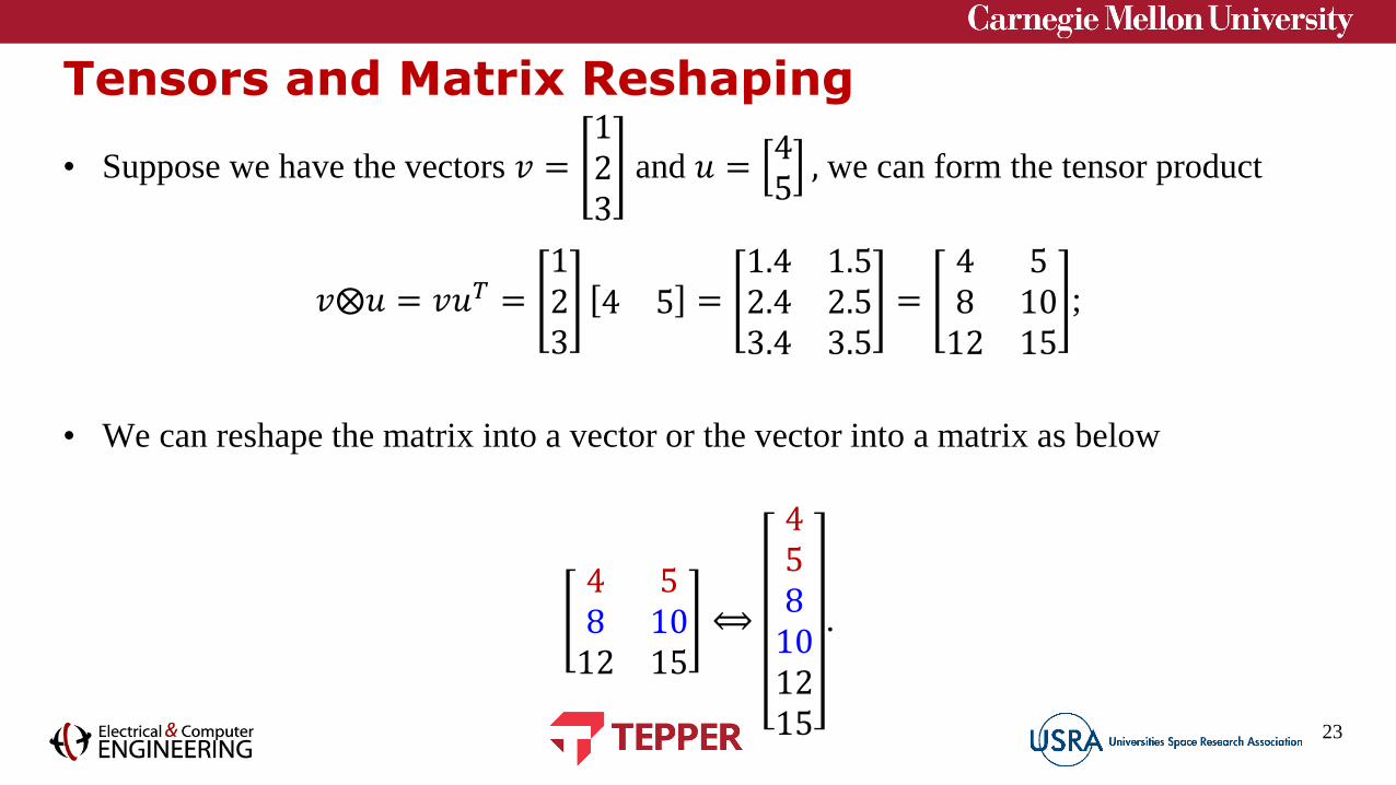
Tensors and Matrix Reshaping

• Suppose we have the vectors 𝑣 =123

and 𝑢 =45, we can form the tensor product

𝑣⨂𝑢 = 𝑣𝑢𝑇 =123

4 5 =1.4 1.52.4 2.53.4 3.5

=4 58 1012 15

;

• We can reshape the matrix into a vector or the vector into a matrix as below

4 58 1012 15

⟺

458101215

.

23

Tensors and Composite States

• Suppose we have the two basis vectors: |0 > in 𝐻1and |1 > in 𝐻2, where 𝐻1 and 𝐻2are the respective Hilbert spaces. What is the basis for the combined Hilbert space

𝐻 = 𝐻1⨂𝐻2?

• Using what we have learned so far, the basis for the combined Hilbert space can be

written as all the possible products of the basis states for 𝐻1 and 𝐻2, thus

|0 > ⨂ |0 > = |00 >, |0 > ⨂ |1 > = |01 >, |1 > ⨂|0 > = |10 >, |1 > ⨂|1 > = |11 >;

• In a more general example, given the state 𝜓 = 𝑎1 𝑥 > +𝑎2 𝑦 > with basis vectors

|𝑥 > and |𝑦 > in 𝐻1 and the state 𝜑 > = 𝑏1 𝑢 > +𝑏2|𝑣 > with the basis vectors |𝑢 >and |𝑣 > in 𝐻2 one can create the combined Hilbert space 𝐻1⨂𝐻2 where the new state

is described by

|𝜒 > = 𝜓⨂𝜑 = 𝑎1 𝑥 > +𝑎2 𝑦 > ⨂ 𝑏1 𝑢 > +𝑏2 𝑣 >

⟹ 𝜒 >= 𝑎1𝑏1 𝑥 > ⨂ 𝑢 > +𝑎1𝑏2 𝑥 > ⨂ 𝑣 > +𝑎2𝑏1 𝑦 > ⨂ 𝑢 > +𝑎2𝑏2 𝑦 > ⨂𝑣 >.

24

Tensors and Process-State Duality

• We learned that 𝑣⨂𝑢 can also be a matrix, which is a mathematical process (operator)

representing a linear transformation, but we also found that 𝑣⨂𝑢 is an abstract vector,

which represents a state of a system;

• Evidently matrices encode processes and vectors encode states;

• We can therefore view the tensor product 𝑉⨂𝑈 as either a process or a state simply by

reshaping the numbers as a rectangle or a list;

• By generalizing the idea of processes to higher dimensional arrays, we get tensors that

can be constructed to create tensor networks;

25

Graphical Perspective of a Tensor Product• We previously created a tensor 𝑢⨂𝑣 out of the two vectors 𝑢 and 𝑣 as illustrated below;

• Another way to look at this process is by examining the interactions between the “nodes” that

perform the multiplication or computation of the product; this perspective leads to the graphical

illustration alongside the vector tensor multiplication;

• The graphical perspective is reminiscent of artificial neural network interconnections; in fact,

this perspective illuminates a computational scheme known as “tensor flow”.

26

Operators and Tensors

• Given and operator 𝐴 that acts on |𝜓 > in 𝐻1 and an operator 𝐵 that acts on |𝜑 > in 𝐻2,

we can create an operator 𝐴⨂𝐵 that acts on the vectors in the combined vector space

𝐻1⨂𝐻2, thus

(𝐴⨂𝐵)( 𝜓 > ⨂ 𝜑 >) = 𝐴 𝜓 > ⨂𝐵 𝜑 >;

• If the two operators 𝐴 and 𝐵 are given as the matrices

𝐴 =𝑎 𝑏𝑐 𝑑

and 𝐵 =𝑒 𝑓𝑔 ℎ

, we calculate the tensor product as

𝐴⨂𝐵 =𝑎𝐵 𝑏𝐵𝑐𝐵 𝑑𝐵

=

𝑎𝑒 𝑎𝑓 𝑏𝑒 𝑏𝑓𝑎𝑔 𝑎ℎ 𝑏𝑔 𝑏ℎ𝑐𝑒 𝑐𝑓 𝑑𝑒 𝑑𝑓𝑐𝑔 𝑐ℎ 𝑑𝑔 𝑑ℎ

Eqn. (3.18).

27

Describing Quantum Particle Interactions with Tensors

• Quantum particles, such as atoms, ions, electrons, and photons, can be manipulated to

perform some computing; the catch is that we must describe these particles interact with one

another;

• We may need to know what these particles are doing, what their status (state) is, in how

many ways they are interacting, or what the probability of their being in certain states is; the

state of a quantum particle can be described by a complex unit vector in 𝐂𝑛;

• The combined state of two particles, one described by a basis vector 𝑣1, in 𝐂𝑛and the other

by 𝑣2 in 𝐂𝑛 is a tensor product of their individual Hilbert spaces; thus

𝐂𝑛 ⊗𝐂𝑛;

• As we discussed previously, the resulting basis vectors of the combined Hilbert space can

be thought of as a matrix, called the density matrix, 𝜌;

• For N particles, density matrix 𝜌 is on 𝐶𝑛⨂𝐶𝑛⨂𝐶𝑛…⨂𝐶𝑛 = 𝐶𝑛 𝑁 Eqn. (3.19).

28

SVD of a Complex Matrix : Schmidt Decomposition

• When matrix 𝑀 is complex, as in quantum mechanical operators, then 𝑀 = 𝑈Λ𝑉†;

• If we write the columns of 𝑈 as 𝑢𝑖 and those of 𝑉 as 𝑣𝑖, then

𝑀 =. | .. 𝑢𝑖 .. | .

⋱𝜎𝑖

⋱

− − 𝑣𝑖 − − = 𝜎1𝑢1𝑣1† + 𝜎2𝑢2𝑣2

† +⋯+ 𝜎𝑟𝑢𝑟𝑣𝑟†

Eqn. (3.20);

• Recall that 𝑢𝑣𝑇 = 𝑢⨂𝑣 = |𝑢 >< 𝑣|; because of this, (3.20) above can be written as

(3.21) below;

• Matrix 𝑀 can be written as state a |𝜓 > = 𝜎1𝑢1⨂𝑣1 + 𝜎2𝑢2⨂𝑣2 +⋯+ 𝜎𝑟𝑢𝑟⨂𝑣𝑟⟹ |𝜓 >= σ𝑖=1

𝑟 𝜎𝑖𝑢𝑖⨂𝑣𝑖 Eqn. (3.21).

29

SVD of a Complex Matrix and Quantum Entanglement

• When we decompose a complex matrix 𝑀 we can write it as state vector

|𝜓 > = σ𝑖=1𝑟 𝜎𝑖𝑢𝑖⨂𝑣𝑖 Eqn. (3.21);

• The singular values 𝜎𝑖 are renamed the Schmidt coefficients, and the rank of the matrix

𝑀 (which is the number of non-zero singular values) 𝑟, is renamed the Schmidt rank;

• Quantum state vector |𝜓 > now represents entanglement when the Schmidt rank 𝑟 > 1;however, the system is not entangled when the rank is not larger than 1;

• Quantum entanglement is a resource in quantum computing and communication.

30

• Reviewed complex linear algebra relevant for quantum mechanics (used in quantum

computing and communication applications);

– Complex vectors

– Complex matrices

• Introduced the notion of tensor product

– A way to interconvert between vectors and matrices and vice versa

– Briefly introduced (mathematically) the idea of entanglement

31

Summary