Algebra II - North Stonington Public Schools

Algebra II

A.REI.D.10 Understand that the graph of an equation in two variables is the set of all its solutions

plotted in the coordinate plane, often forming a curve (which could be a line).

A.REI.D.11 Explain why the x-coordinate of the points where the graphs of the equations y = f(x)

and y = g(x) intersect are the solutions of the equation f(x) = g(x); find the solutions

approximately, e.g., using technology to graph the functions, make tables of values, or

find successive approximations. Include where f(x) and/or g(x) are linear, rational,

absolute value, exponential and logarithmic functions.

A.REI.D.12 Graph the solutions to a linear inequality in two variables as a half plane (excluding the

boundary in the case of a strict inequality) and graph the solution set of a system of

linear inequalities as the intersection of the corresponding half-planes.

A.CED.2 Create equations in two or more variables to represent relationships between quantities;

graph equations on coordinate axes with labels and scales.

F.IF.1 Understand that a function from one set (called the domain) to another set (called the

range) assigns to each element of the domain exactly one element of the range. If f is a

function and x is an element of its domain, then f(x) denotes the output of f

corresponding to the input x. The graph of f is the graph of the equation y = f(x).

F.IF.2 Use function notation, evaluate functions for inputs in their domains, and interpret

statements that use function notation in terms of a context

F.IF.5 Relate the domain of a function to its graph and, where applicable, to the quantitative

relationship it describes. For example, if the function h(n) gives the number of person-

hours it takes to assemble n engines in a factory, then the positive integers would be an

appropriate domain for the function.

COURSE OUTLINE

Unit One Functions and Inverse

Functions

30 Days

Unit Two Quadratic Functions 25 Days

Unit Three Polynomial Functions 30 Days

Unit Four Rational and Power

Functions

25 Days

Unit Five Exponential and Logarithmic

Functions

30 Days

Unit Six Sequences and Series 20 Days

School-wide Academic Expectations Taught In This Course

o Analysis

o Collaboration

o Communication

o Literacy

School-wide Social and Civic Expectations Taught in This Course

o Demonstrate Resiliency

o Demonstrate Responsibility

o Demonstrate Respect

Content Standards Taught in This Course

F.IF.7 Graph functions expressed symbolically and show key features of the graph, by hand in

simple cases and using technology for more complicated cases.

F.IF.7b Graph square root, cube root, and piecewise-defined functions, including step functions

and absolute value functions.

F.IF.9 Compare properties of two functions each represented in a different way (algebraically,

graphically, numerically in tables, or by verbal descriptions). For example, given a graph

of one quadratic function and an algebraic expression for another, say which has the

larger maximum.

F.BF.1b Combine standard function types using arithmetic operations.

F.BF.1c (+) Compose functions. For example, if T(y) is the temperature in the atmosphere as a

function of height, and h(t) is the height of a weather balloon as a function of time, then

T(h(t)) is the temperature at the location of the weather balloon as a function of time.

F.BF.3 Identify the effect on the graph of replacing f(x) by f(x) + k, kf(x), f(kx), and f(x + k) for

specific values of k (both positive and negative); find the value of k given the graphs.

Experiment with cases and illustrate an explanation of the effects on the graph using

technology. Include recognizing even and odd functions from their graphs and algebraic

expressions for them.

F.BF.4 Find inverse functions.

F.BF.4a Solve an equation of the form f(x) = c for a simple function f that has an inverse and

write an expression for the inverse. For example, f(x) = 2(x3) for x > 0 or f(x) = (x +

1)/(x – 1) for x ≠ 1 (x not equal to 1).

F.BF.4b (+) Verify by composition that one function is the inverse of another.

F.BF.4c (+) Read values of an inverse function from a graph or a table, given that the graph has an

inverse.

A.SSE.3 Choose and produce an equivalent from of an expression to reveal and explain

properties of the quantity represented by the expression.

A.SSE.3a Factor a quadratic expression to reveal zeros of the function it defines.

A.SSE.3b Complete the square in a quadratic expression to reveal the maximum/minimum

value of the function it defines.

A.REI.A.2 Solve simple rational and radical equations in one variable, and give examples

showing how extraneous solutions may arise.

A.REI.4 Solve quadratic equations in one variable.

A.REI.4b Solve quadratic equations by inspection (e.g., for x2 = 49), taking square roots,

completing the square, the quadratic formula and factoring, as appropriate to the initial

form of the equation. Recognize when the quadratic formula gives complex solutions

and write them as 𝑎 ± 𝑏𝑖 for real numbers a and b.

BF.A.1 Write a function that describes a relationship between two quantities.

CED.A.1 Create equations and inequalities in one variable and use them to solve problems.

Include equations arising from linear and quadratic functions, and simple rational and

exponential functions.

CED.A.2 Create equations in two or more variables to represent relationships between

quantities; graph equations on coordinate axes with labels and scales.

F.IF.B.4 For a function that models a relationship between two quantities, interpret key

features of graphs and tables in terms of the quantities, and sketch graphs showing key

features given a verbal description of the relationship. Key features include: intercepts;

intervals where the function is increasing, decreasing, positive, or negative; relative

maximums and minimums; symmetries; end behavior; and periodicity.

F.IF.C.7 Graph functions expressed symbolically and show key features of the graph, by

hand in simple cases and using technology for more complicated cases.

F.IF.C.7a Graph linear and quadratic functions and show intercepts, maxima, and minima.

F.IF.C.7b Graph square root, cube root, and piecewise-defined functions, including step

functions and absolute value functions.

N.CN.1 Know there is a complex number i such that 𝑖2 = √−1, and every complex

number has the form a + bi with a and b real.

N.CN.2 Use the relation i2 = -1 and the commutative, associative, and distributive

properties to add, subtract, and multiply complex numbers.

N.CN.7 Solve quadratic equations with real coefficients that have complex solutions.

N.CN.9 (+) Know the Fundamental Theorem of Algebra; show that it is true for quadratic

polynomials. (Note that only functions with real coefficients are considered in this

investigation.)

N.RN.3 Explain why the sum or product of two rational numbers is rational and the sum of a

rational and an irrational number is irrational; and that the product of a nonzero rational

number and an irrational number is irrational.

F.IF.7c Graph polynomial functions, identifying zeros when suitable factorizations are available,

and showing end behavior.

F.IF.4 For a function that models a relationship between two quantities, interpret key features

of graphs and tables in terms of the quantities, and sketch graphs showing key features

given a verbal description of the relationship. Key features include: intercepts; intervals

where the function is increasing, decreasing, positive, or negative; relative maxima and

minima; multiplicity of roots; symmetries; end behavior; and periodicity.

A.APR.1 Understand that polynomials form a system analogous to the integers, namely, they are

closed under the operations of addition, subtraction, and multiplication; add, subtract,

and multiply polynomials.

A.APR.2 Know and apply the Remainder Theorem: For a polynomial p(x) and a number a, the

remainder on division by x – a is p(a), so p(a) = 0 if and only if (x – a) is a factor of p(x).

A.APR.3 Identify zeros of polynomials when suitable factorizations are available, and use the

zeros to construct a rough graph of the function defined by the polynomial.

A.SSE.2 Use the structure of an expression to identify ways to rewrite it. For example, see x4 – y4

as (x2)2 – (y2)2, thus recognizing it as a difference of squares that can be factored as (x2–

y2)• (x2 + y2).

A.APR.4 Prove polynomial identities and use them to describe numerical relationships. For

example, the polynomial identity (x2 + y2)2 = (x2 – y2)2 + (2xy)2 can be used to generate

Pythagorean triples.

A.APR.5 (+) Know and apply that the Binomial Theorem gives the expansion of (x + y)n

in powers

of x and y for a positive integer n, where x and y are any numbers, with coefficients

determined for example by Pascal’s Triangle. (The Binomial Theorem can be proved by

mathematical induction or by a combinatorial argument.)

F.LE.3 Observe using graphs and tables that a quantity increasing exponentially eventually

exceeds a quantity increasing linearly, quadratically, or (more generally) as a polynomial

function.

A.SSE.1 Interpret expressions that represent a quantity in terms of its context.

A.SSE.1b Interpret complicated expressions by viewing one or more parts as a single entity.


of graphs and tables in terms of the quantities and sketch graphs showing key features

given a verbal description of the relationship.

F.IF.7d(+) Graph rational functions, identifying zeros and asymptotes when suitable factorizations

are available, and showing end behavior.

A.CED.3 Represent constraints by equations or inequalities, and by systems of equations and/or

inequalities, and interpret solutions as viable or non-viable in a modeling context.

A.APR.1b Rewrite simple rational expressions in different forms; write a(x)/b(x) in the form q(x) +

r(x)/b(x), where a(x), b(x), q(x), and r(x) are polynomials with the degree of r(x) less

than the degree of b(x), using inspection, long division, or, for more complicated

examples, a computer algebra system.

A.APR.6 Rewrite simple rational expressions in different forms; write a(x)/b(x) in the form q(x) +




A.APR.7(+) Understand that rational expressions form a system analogous to the rational numbers,

closed under addition, subtraction, multiplication, and division by a nonzero rational

expression; add, subtract, multiply, and divide rational expressions.

A.REI.2 Solve simple rational and radical equations in one variable, and give examples showing

how extraneous roots may arise.

A.REI.11b Explain why the x-coordinates of the points where the graphs of the equations y = f(x)

and y = g(x) intersect are the solutions of the equations f(x) = g(x); find the solutions

approximately, e.g. using technology to graph the functions, make tables of values, or

find successive approximations. Include cases where f(x) and/or g(x) are linear,

polynomial, rational, absolute value, exponential, and logarithmic functions.


A-SSE-1b Interpret complicated expressions by viewing one or more of their parts as a single

entity. For example, interpret 𝑃(1 + 𝑟)𝑛 as a product of P and a factor not depending on

P.

A-SSE-4 Derive the formula for the sum of a finite geometric series (when the common ratio is

not 1), and use the formula to solve problems. For example, calculate mortgage

payments.

A-CED-1 Create equations and inequalities in one variable and use them to solve problems.



A-CED-2 Create equations in two or more variables to represent relationships between quantities;


F-IF. 7e Graph exponential and logarithmic functions, showing intercepts and end behavior, and

trigonometric functions, showing period, midline, and amplitude.

F-IF-8 Write a function defined by an expression in different but equivalent forms to reveal and

explain different properties of the function.

F-BF-3 Identify the effect on the graph of replacing 𝑓(𝑥) by 𝑓𝑘, 𝑘𝑓(𝑥), 𝑓(𝑘𝑥),

and 𝑓(𝑥 + 𝑘) for specific values of 𝑘 (both positive and negative);

find the values of k given the graphs. Experiment with cases and illustrate an

explanation of the effects on the graph using technology. Include recognizing even and

odd functions from their graphs and algebraic expressions for them.

F-BF-5 (+) Understand the inverse relationship between exponents and logarithms and use this

relationship to solve problems involving logarithms and exponents.

F-LE-4 For exponential models, express as a logarithm the solution to 𝑎𝑏(𝑐𝑡) = 𝑑 where a, c and

d are numbers and the base b is 2, 10 or e; evaluate the logarithm using technology.

F-LE-5 Interpret the parameters of an exponential function in terms of a context.






F-IF.A.3 Recognize that sequences are functions, sometimes defined recursively, whose domain

is a subset of the integers. For example, the Fibonacci sequence is defined recursively by

f(0) = f(1) = 1, f(n+1) = f(n) + f(n-1) for n ≥ 1.

F-BF.A.2 Write arithmetic and geometric sequences both recursively and with an explicit formula,

use them to model situations, and translate between the two forms.

F-LE.A.2 Construct linear and exponential functions, including arithmetic and geometric

sequences, given a graph, a description of a relationship, or two input-output pairs

(include reading these from a table).

A-SSE.B.4 Derive the formula for the sum of a finite geometric series (when the common ratio is


payments.

F-BF.A.1a Determine an explicit expression, a recursive process, or steps for calculation from a

context.

SL.9-10.1.c Propel conversations by posing and responding to questions that relate the current

discussion to broader themes or larger ideas; actively incorporate others into the

discussion; and clarify, verify, or challenge ideas and conclusions.

http://www.corestandards.org/ELA-Literacy/SL/9-10/1/c/

Unit 1: Functions and Inverse Functions

Introduction and Established Goals: This Unit serves as both a review and an extension of functions

from Algebra 1. Students will be familiar with functions, particularly linear functions, from Algebra 1.

These subjects are reviewed in new contexts, such as linear programming and conic sections. The Unit

then extends students’ understanding of functions by examining the important concepts of function

growth, transformation of functions, creating new functions from old, and inverse functions. This Unit

sets the groundwork for the rest of Algebra 2 by investigating functions in a general way which is then

applied as needed later in the curriculum. As many of the ideas in this Unit review concepts introduced

in Algebra 1, there is an emphasis throughout Unit 1 on some of the applications of these ideas to

realistic contexts.

Desired Outcome(s):

A function is a special kind of relation where each member of the domain of the function is

associated with exactly one member of the range of the function.

We can study a very wide range of phenomena by starting with a very small group of “parent”

functions and applying transformations to those functions.

CT State Standard(s):

A.REI.D.10 Understand that the graph of an equation in two variables is the set of all its solutions

plotted in the coordinate plane, often forming a curve (which could be a line).

A.REI.D.11 Explain why the x-coordinate of the points where the graphs of the equations y = f(x)

and y = g(x) intersect are the solutions of the equation f(x) = g(x); find the solutions

approximately, e.g., using technology to graph the functions, make tables of values, or

find successive approximations. Include where f(x) and/or g(x) are linear, rational,

absolute value, exponential and logarithmic functions.

A.REI.D.12 Graph the solutions to a linear inequality in two variables as a half plane (excluding the

boundary in the case of a strict inequality) and graph the solution set of a system of

linear inequalities as the intersection of the corresponding half-planes.



F.IF.1 Understand that a function from one set (called the domain) to another set (called the

range) assigns to each element of the domain exactly one element of the range. If f is a

function and x is an element of its domain, then f(x) denotes the output of f

corresponding to the input x. The graph of f is the graph of the equation y = f(x).

F.IF.2 Use function notation, evaluate functions for inputs in their domains, and interpret

statements that use function notation in terms of a context

F.IF.5 Relate the domain of a function to its graph and, where applicable, to the quantitative

relationship it describes. For example, if the function h(n) gives the number of person-

hours it takes to assemble n engines in a factory, then the positive integers would be an

appropriate domain for the function.



F.IF.7b Graph square root, cube root, and piecewise-defined functions, including step functions

and absolute value functions.


graphically, numerically in tables, or by verbal descriptions). For example, given a graph


larger maximum.

F.BF.1b Combine standard function types using arithmetic operations.

F.BF.1c (+) Compose functions. For example, if T(y) is the temperature in the atmosphere as a

function of height, and h(t) is the height of a weather balloon as a function of time, then

T(h(t)) is the temperature at the location of the weather balloon as a function of time.

F.BF.3 Identify the effect on the graph of replacing f(x) by f(x) + k, kf(x), f(kx), and f(x + k) for

specific values of k (both positive and negative); find the value of k given the graphs.

Experiment with cases and illustrate an explanation of the effects on the graph using

technology. Include recognizing even and odd functions from their graphs and algebraic

expressions for them.

F.BF.4 Find inverse functions.


write an expression for the inverse. For example, f(x) = 2(x3) for x > 0 or f(x) = (x +

1)/(x – 1) for x ≠ 1 (x not equal to 1).



inverse.




Common Core Standard(s):

MP5: Use appropriate tools strategically

MP4: Look for and make use of structure

Essential Question(s):

What is a function?

What are the different ways in which functions may be represented?

How do we find an optimal solution to a linear programming problem?

What is the meaning of the domain and range of a function?

What is a family of functions?

How do different families of functions grow?

What is the effect of a transformation of an independent variable? What is the effect of a

transformation of a dependent variable?

(+) What does it mean to compose two functions?

What is the inverse of a function? How can functions be used to model real world situations, make predictions, and solve problems?

Key Terms/Concepts: Absolute value function, Algorithm, Angle of a generator, Area of a circle,

Axis of symmetry, Boundary line, Circle, Circumference, Composition of functions, Constraint,

Dependent variable, Depreciation, Directrix, Domain, Ellipse, Equivalent equation and inequality, Even

function, Exponential function, Family of functions, Feasible region, Floor function, Foci of an ellipse,

hyperbola, or parabola, Function, Function notation, Greatest integer function, Half-plane, Horizontal

and vertical axes, Horizontal line test, Horizontal shift/translation, Hyperbola, Independent variable,

Inequality, Input and output of a function, Inside change, Inverse function, Isometry, Line symmetry,


Linear growth, Major axis/minor axis of an ellipse, Maximum/minimum, Natural domain, Nonlinear

growth, Objective function, Odd function, One-to-one function, Optimization, Ordered pair, Origin,

Outside change, Parabola, Parameter, parent function, Piecewise function, Quadratic function,

Quadritium, Radius of a circle, Range, Reflection, Relation, Restricted domain, Root function,

Rotational symmetry, Shading, Solution of a system of linear equations, Solution of a system of linear

inequalities, Standard form, Slope, Step function, Symmetric with respect to the origin, Symmetric with

respect to the y-axis, System of equations, System of inequalities, Test point, Transformation, Vertex,

Vertical stretch, Vertical shift/translation

LEARNING PLAN STANDARD LEARNING OBJECTIVES

(Content and Skill)

INSTRUCTIONAL

STRATEGIES

ASSESMENT

EVIDENCE

A.REI.D.10

A.REI.D.11

A.REI.D.12

SL.9-10.1.c

1. Students will graph the

solution set of a linear

system of inequalities in

two variables as the

intersection of the

corresponding system of

half-planes, and interpret

the result.

2. Students will be able to

define an objective

function for a given

context.


use the seven step linear

programming algorithm

to identify optimal

solutions to practical

problems.


use linear programming

to identify optimal

solutions to practical

problems.

o Activity 1.1.1 Keeping the

Peace

Exit Slip 1.1

Quiz o Activity 1.1.2 Peacekeeping

Problem: Area Constraint

o Activity 1.1.3: Finding the

Objective Function

o Activity 1.1.4 Exploring Corner

Points

o Activity 1.1.5 The Rationale for

Only Evaluating at Corner

Points

o Activity 1.1.6 Meera’s Jobs

o Activity 1.1.7 The Farmer

o Activity 1.1.8 Farm Subsidies

o Activity 1.1.9 Natasha’s Cat

o Activity 1.1.10 Additional

Linear Programming Problems

F.IF.1

F.IF.2

F.IF.5

SL.9-10.1.c

5. Be able to determine if a

given relation is a function

or not.

6. Given a function, be able

to determine its domain

and range.

7. Be able to represent a

function by an equation,

table, graph, or verbal

description and move

o Activity 1.2.1 Function Review Exit Slip 1.2

o Activity 1.2.2 What’s

Reasonable?

o Activity 1.2.3a Function

Junction

o Activity 1.2.3b Is the Function

1-1?

o Activity 1.2.4 Are Conics

Functions?


comfortably from one

representation to another.

8. Determine the

reasonableness of the

domain and range of a

function in a realistic

context.

9. Determine whether a

function is a 1-1 function

from a graph or table of

values.

10. Determine whether the

basic conic sections are

functions or not.

F.IF.7B

SL.9-10.1.c

11. Be able to identify

different types of growth

using a table

12. Be able to graph and

analyze the absolute value

function

13. Be able to graph and

analyze the piecewise and

step functions

14. Understand end behavior

of even and odd functions

o Activity 1.3.1 Linear and

Nonlinear Growth

Exit Slip 1.3.1

Exit Slip 1.3.2

Quiz

o Activity 1.3.2 The Absolute

Value Function

o Activity 1.3.3 Piecewise and

Step Functions

o Activity 1.3.4 Symmetry

Review

o Activity 1.3.5 Even and Odd

Functions

F.BF.1b

F.BF.3

SL.9-10.1.c

15. Given two functions f(x)

and g(x), be able to find

f + g, f – g, fg, and f ÷ g

symbolically and for f +

g and f – g graphically.

16. Represent a verbal

description of a function

transformation

symbolically.

17. Understand the

difference between a

transformation of an

independent variable and

a dependent variable.

18. Given a function f(x), be

able to describe the

effects of the

transformations f(x) + k,

o Activity 1.4.1 Putting Functions

Together (Pt 1 and 2)

Exit Slip 1.4

o Activity 1.4.2 Inside Change,

Outside Change (Pt 1 and 2)

o Activity 1.4.3 Move It! Pt 1

o Activity 1.4.4 Stretch It! Pt 1

o Activity 1.4.5 Transformations

Made Easy

o Activity 1.4.6 Greenhouse Gas

Emissions

f(x + k), and kf(x) for a

constant k.

19. Given a graph of a

function and a

transformation of that

function, be able to

determine the

transformation that is

represented in the graph.

20. Given a graph of a

function, be able to

graph (by hand) a

transformation of that

function.

F.BF.1c (+)

SL.9-10.1.c


compose functions using

one or more arithmetic

operation

o Activity 1.5.1 Composing

Composite Functions

Exit Slip 1.5

o Activity 1.5.2 Domains and

Graphs of Composite

FUNctions

o Activity 1.5.3 Composition of

Function Applications

F.BF.4

SL.9-10.1.c

22. Students will verify which

functions have inverses

23. Students will use

composition techniques to

find equations of inverse

functions

o Activity 1.6.1 Functions and

their Inverses

Exit Slip 1.6

o Activity 1.6.2 Finding Inverses

o Activity 1.6.3 Using Functions

and their Inverses

o Activity 1.6.4 Are You My

Inverse?

F.BF.4

SL.9-10.1.c

24. Students will find

equations for the inverses

of power functions

o Activity 1.7.1 Review of

Exponents

Exit Slip 1.7

o Activity 1.7.2 Inverses of

Power Functions

o Activity 1.7.3 Tuning Up

Performance

Task

End of Unit Test

Suggested Resources and Texts:

https://screen.yahoo.com/u-troops-head-ebola-hot-163128163.html? Activity 1.1.1

Green and red pencils for plotting the solutions and non solutions in Activity 1.1.1, and Activity

1.1.2A and 1.1.2B

http://people.richland.edu/james/ictcm/2006/slope.html (1.1.5)

Belgian Chocolates and Tomato Farmers videos (produced by Mathematics to Enhance

Economics: Enhancing Teaching and Learning – at

www.metalproject.co.uk/METAL/Resources/Films/linear_programming/index.html (1.6)

The following website may be used to give insight into who is using linear programming and

why: http://www.ilog.com/products/optimization/. (anytime after 1.1.5)

https://screen.yahoo.com/u-troops-head-ebola-hot-163128163.html

http://people.richland.edu/james/ictcm/2006/slope.html

http://www.metalproject.co.uk/METAL/Resources/Films/linear_programming/index.html

See www.hsor.org for many high school linear programming problems and information on

linear programming (1.5)

Contemporary College Algebra: Data, Functions, Modeling, 6th ed., McGraw – Hill Primis

Custom Publishing . Don Small author (Farm Subsidy problem, 1.1.9)

Farm subsidy data base at http://farm.ewg.

org/farm/region.php?fips=09003 (1.6)

video on Operational Research use in 1.6 or later- http://www.bnet.com/2422-13950_23-

178846.html

http://illuminations.nctm.org (supplemental problem #3)

http://www.wikihow.com/Make-a-Duct-Tape-Wallet

http://www.ducttapefashion.com/products/prod01.htm (supplemental problem #4)

TI Numb3rs Linear Programming Activity at

http://education.ti.com/educationportal/activityexchange/Activity.do?cid=US&aId=7508

(supplemental problem #6)

Bakers Choice published by Key Curriculum Press (supplemental problem #7)

Information relevant to George Dantzig: http://www.lionhrtpub.com/orms/orms-8-

05/dantzig.html and http://www.lionhrtpub.com/orms/orms-6-05/dantzig.html (Suggested

research question #4)

Suggested Technology: Graphing calculator, Projector, Access to internet

http://www.hsor.org/

http://farm.ewg/

https://mail.wcsu.edu/owa/redir.aspx?C=5deda06d8de846579753f0ed1e80a694&URL=http%3a%2f%2fwww.bnet.com%2f2422-13950_23-178846.html

https://mail.wcsu.edu/owa/redir.aspx?C=5deda06d8de846579753f0ed1e80a694&URL=http%3a%2f%2fwww.bnet.com%2f2422-13950_23-178846.html

http://illuminations.nctm.org/

http://www.wikihow.com/Make-a-Duct-Tape-Wallet

http://www.ducttapefashion.com/products/prod01.htm

http://education.ti.com/educationportal/activityexchange/Activity.do?cid=US&aId=7508

http://www.lionhrtpub.com/orms/orms-8-05/dantzig.html



Unit 2: Quadratic Functions

Introduction and Established Goals: Quadratic functions are the first family of functions that

students will examine in depth in this Algebra 2 curriculum. Students will apply their knowledge of the

effects that different transformations have on the graph of a function to the study of quadratic functions.

In particular, students will examine the effects of vertical and horizontal shifts, vertical stretches, and

reflections over the x-axis and their effects on properties of quadratic functions.

Mastery of the unit will require students to develop their understanding of: (1) properties of quadratic

functions based on the parameters a, b and c in the standard form of the quadratic function 𝑓(𝑥) =𝑎𝑥2 + 𝑏𝑥 + 𝑐, and the parameters a, h and k in the vertex form of the quadratic function 𝑓(𝑥) =𝑎(𝑥 − ℎ)2 + 𝑘; (2) different methods for solving quadratic equations; (3) the nature of the roots of a

quadratic equation based on the value of the discriminant; (4) the imaginary number i and operations

involving complex numbers (5) complex conjugates as solutions of quadratic equations with a negative

discriminant; (6) the Fundamental Theorem of Algebra in relation to quadratic functions; (7) modeling

using quadratic functions; and (9) solving radical equations.

This unit builds on Unit 8 of the Common Core Algebra 1 Curriculum, providing students a deeper

conceptual and procedural understanding of quadratic functions. The coverage of material in this unit

will depend on the extent to which students studied and acquired quadratic function competencies in

Algebra I. Throughout this unit, authors will highlight the connections between activities in this unit

and activities in Unit 8 of the Algebra 1 curriculum, detailing the specific Algebra 1 activities that serve

as the foundation of Algebra 2 activities.

Desired Outcome(s):

Students will understand quadratic functions can be used to model real world relationships and

the key points in quadratic functions have meaning in the real world context.

Students will use dynamic software, graphing calculators, and other technology to explore and

deepen their understanding of mathematics.


A.SSE.3 Choose and produce an equivalent from of an expression to reveal and explain

properties of the quantity represented by the expression.

A.SSE.3a Factor a quadratic expression to reveal zeros of the function it defines.

A.SSE.3b Complete the square in a quadratic expression to reveal the maximum/minimum

value of the function it defines.

A.REI.A.2 Solve simple rational and radical equations in one variable, and give examples

showing how extraneous solutions may arise.

A.REI.4 Solve quadratic equations in one variable.

A.REI.4b Solve quadratic equations by inspection (e.g., for x2 = 49), taking square roots,

completing the square, the quadratic formula and factoring, as appropriate to the initial

form of the equation. Recognize when the quadratic formula gives complex solutions

and write them as 𝑎 ± 𝑏𝑖 for real numbers a and b.

BF.A.1 Write a function that describes a relationship between two quantities.

CED.A.1 Create equations and inequalities in one variable and use them to solve problems.



CED.A.2 Create equations in two or more variables to represent relationships between

quantities; graph equations on coordinate axes with labels and scales.

F.IF.B.4 For a function that models a relationship between two quantities, interpret key

features of graphs and tables in terms of the quantities, and sketch graphs showing key

features given a verbal description of the relationship. Key features include: intercepts;

intervals where the function is increasing, decreasing, positive, or negative; relative

maximums and minimums; symmetries; end behavior; and periodicity.

F.IF.C.7 Graph functions expressed symbolically and show key features of the graph, by

hand in simple cases and using technology for more complicated cases.

F.IF.C.7a Graph linear and quadratic functions and show intercepts, maxima, and minima.

F.IF.C.7b Graph square root, cube root, and piecewise-defined functions, including step

functions and absolute value functions.

N.CN.1 Know there is a complex number i such that 𝑖2 = √−1, and every complex

number has the form a + bi with a and b real.

N.CN.2 Use the relation i2 = -1 and the commutative, associative, and distributive

properties to add, subtract, and multiply complex numbers.

N.CN.7 Solve quadratic equations with real coefficients that have complex solutions.

N.CN.9 (+) Know the Fundamental Theorem of Algebra; show that it is true for quadratic

polynomials. (Note that only functions with real coefficients are considered in this

investigation.)

N.RN.3 Explain why the sum or product of two rational numbers is rational and the sum of a

rational and an irrational number is irrational; and that the product of a nonzero rational

number and an irrational number is irrational.





MP 3: Construct viable arguments and critique the reasoning of others.

MP 4: Model with mathematics

MP 7: Look for and make use of structure


How do I describe quadratic functions in terms of transformations?

How do I describe quadratic functions in terms of properties such as concavity and end behavior?

How do I solve a quadratic equation?

How can I determine the nature of the roots of a quadratic equation based on the value of the discriminant?

What is the definition of the imaginary number i?

What is the structure of the complex numbers?

What is the Fundamental Theorem of Algebra, and what is its relation to quadratic functions?

How do I use quadratic functions as mathematical models?

How do I solve radical equations?

Key Terms/Concepts:

Absolute value, Axis of symmetry, Binomial, Binomial expansion, Closed sets, Closure of sets under

an operation, Completing the square, Complex conjugate, Complex number, Concave up/down, Cost

function, Decreasing function, Distributive property, End behavior, Extraneous root, Extraneous

solution, Factor, Factor a quadratic over the integers, Family of functions, Imaginary number,


Increasing function, Infinity, Inside change, Mathematical model(ing), Modeling diagram, Monomial,

Outside change, Parabola, Parabolic, Parametric equations, Parent function, Piecewise defined function,

Profit function, Quadratic formula, Quadratic function, Quadratic regression, Radical equation,

Radicand, Revenue function, Root, Sets of numbers {Natural numbers, Whole numbers, Integers,

Rationals, Irrationals, Real numbers, Complex numbers}, Slope, Solution, Square root equation,

Standard form of a quadratic function, Transformation, Vertex, Vertex form of a quadratic function, x-

intercept, y-intercept, zeros of a function.


(Content and Skill)

INSTRUCTIONAL

STRATEGIES

ASSESMENT

EVIDENCE

F.IF.4

F.IF.7

F.IF.7a


describe the graphs of x2 +

k, (x + k)2, kx2, ax2 + bx

+ c, and a(x – h)2 + k,

based on the values of k,

a, b, c, and h.

2. Given a quadratic function,

students will be able to

describe the features of the

function (intercepts,

intervals where it is

positive/negative, intervals

where it is increasing and

decreasing, concavity, axis

of symmetry, and end

behavior).

o Activity 2.1.1: Move It! Part

Two

Exit Slip 2.1.1

Exit Slip 2.1.2

Journal Prompt 1

o Activity 2.1.2: How to Move It!

With Standard and Vertex

Forms

o Activity 2.1.3: Stretch It! Part

Two

o Activity 2.1.4: How to Stretch

It! With Standard and Vertex

Forms

o Activity 2.1.5: How do

quadratic functions behave?

A.SSE.3

A.SSE.3A

A.SSE.3B

A.REI.4

A.REI.4B

F.IF.7B

3. Students will solve

quadratic equations using

the following methods:

graphing, square root

method, factoring,

completing the square, and

the quadratic formula

4. Students will choose

among the various methods

for solving quadratic

functions, and give reasons

for their choices

5. Students will interpret the

meaning of intercepts of a

quadratic in the context of

a real world problem

6. Students will define the

absolute value function as

a piecewise defined

function

o Activity 2.2.1: Product of Two

Lines

Exit Slip 2.2.1

Exit Slip 2.2.2

Exit Slip 2.2.3

Journal Prompt 1

Journal Prompt 2

Journal Prompt 3

o Activity 2.2.2: Multiplying and

Factoring

o Activity 2.2.3: Solve Equations

by Factoring

o Activity 2.2.4: Absolute Value

o Activity 2.2.5: Completing the

Square

o Activity 2.2.6: Deriving the

Quadratic Formula

7. Students will determine

when a quadratic equation

as real number solutions or

not

N.RN.3

N.CN.1

N.CN.2

N.CN.7

8. Identify types of numbers:

natural, whole, integers,

rational, irrational, real,

complex

9. Determine whether a set of

numbers is closed under an

operation

10. Determine whether or not a

number, or sum or product

of numbers is rational or

irrational

11. State the definition of i

12. Express the square root of

a negative number in terms

of i

13. Evaluate in for any natural

number n

14. Identify the real and

imaginary parts of a

complex number, using the

a+bi notation

15. State the conjugate of a

complex number

16. Add, subtract, and multiply

complex numbers

- Solve quadratic equations

that have complex

solutions

17. -State the two solutions in

a+bi form

18. -Given a single complex

solution to a quadratic

equation, give the other

solution.

o Activity 2.3.1: Closure and Sets

of Numbers

Exit Slip 2.3.1

Exit Slip 2.3.2

Exit Slip 2.3.3

Journal Prompt 1

Journal Prompt 2

o Activity 2.3.2: Imaginary

Numbers

o Activity 2.3.3: Complex

Numbers

o Activity 2.3.4: Complex

Solutions to Quadratic

Equations

Mid Unit Test

N.CN.2

N.CN.9

19. Determine the number of

roots of a quadratic

equation based on the

discriminant

20. Determine the sign of the

discriminant of a quadratic

equation given the graph

o Activity 2.4.1: Bungee Jumping Exit Slip 2.4.1

Exit Slip 2.4.2

Journal Prompt 1

Journal Prompt 2

o Activity 2.4.2: Zeros? Real or

Complex?

o Activity 2.4.3: Complex Zeros

o Activity 2.4.4: Putting it All

Together


complex numbers

22. Demonstrate the

Fundamental Theorem of

Algebra

BF.A.1

CED.A.1

CED.A.2

IF.B.4

IF.C.7

IF.C.7A

23. Fit a quadratic function to

data that follows a

quadratic relationship and

use the function to make a

prediction

24. Develop a quadratic

function using algebraic

relationships.

25. Solve contextual problems

involving quadratic

functions.

26. Solve optimization

problems that involve

finding the maximum

value (or minimum value)

of a quadratic function

o Activity 2.5.1: Home Run Ball Exit Slip 2.5.1

Exit Slip 2.5.2

Exit Slip 2.5.3

Journal Entry 1

Journal Entry 2

o Activity 2.5.2: Areas of

Equilateral Triangles

o Activity 2.5.3: Parabolic

Behavior

o Activity 2.5.4: Historic Hotels

REI.A.2

CED.A.1

CED.A.2

IF.B.4

IF.C.7A

IF.C.7B

27. Solve equations involving

one and multiple square

root terms.

28. Solve radical equations

graphically.

29. Determine if a solution

obtained from an equation-

solving process is

extraneous.

30. Model and solve

contextual problems

involving radical

equations.

o Activity 2.6.1: Radical

Functions

Exit Slip 2.6.1

Exit Slip 2.6.2

Exit Slip 2.6.3

Journal Entry 1

Journal Entry 2

o Activity 2.6.2: Solving Radical

Equations

o Activity 2.6.3: Crossing Lake

James

Unit 2

Performance

Task

End of Unit Test

Suggested Resources and Texts: Graph paper, youtube videos, “Three Lessons on Parabolas” by Ben

Ceyanes, Pamela Lockwood, Kristina Gill, NCTM Illuminations activity, “Don’t Teach Technology,

Teach with Technology.”

Suggested Technology: Graphing calculators, computer software with a graphing utility for all

activities, online access, TI emulator, TI-84 TRANSFORM App, Camera

Unit 3: Polynomial Functions

Introduction and Established Goals:

Through their study of quadratic functions, students have begun to recognize properties of the graph of

a function such as the extrema, x- and y-intercepts, symmetry of the graph with respect to a line,

concavity, and end behavior. The study of polynomial functions extends the study of non-linear

functions started with quadratic functions to include functions of the form y = P(x) where P(x) is a

polynomial of degree n ≥ 2.

Mastery of the unit will require students to develop their understanding of: 1) the relationship between

zeros of the polynomial function and the factors of the related polynomial; 2) the x- and y-intercepts of

the function; 3) the end behavior of the y-values of the function as x approaches positive or negative

infinity; 4) the transformations of the graph of y=f(x) when it is reflected over the x- and y-axes and

under what conditions will the function be odd or even, i.e. when f(-x) =- f(x) or when f(-x) = f(x); 5)

relative extrema of polynomial functions and how to interpret such values in the context of real-world

problems; 6) operations involving polynomial expressions, including division of polynomials and the

connection of division to the Division Algorithm, the Remainder Theorem, and the Factor Theorem; 7)

factoring polynomials by various methods including the application of the Remainder Theorem and

advanced polynomial identities; 8) the connection between Binomial Expansion and Pascal’s Triangle;

9) applications of polynomials in modeling real-world functions, including solving counting problems

by using generating functions; and 10) the difference between exponential growth versus growth

modeled by polynomial functions.

The unit includes six investigations through which the topics will be developed. Each investigation has

several activities that develop the objectives of the unit. The activities are designed to allow students to

explore relationships and formulate conjectures related to the basic principles in working with

polynomials. Technology is used in many activities to allow students to manipulate parameters in a

function in order to discover patterns in the behavior of the graph of the function. Most activities are

written to enable students to do use any graphing utility available in their classroom, but many activities

were written using GeoGebra since the algebraic, graphic, and numerical representations of the

polynomial functions are readily available.

Desired Outcome(s):

The exponential growth family will always overtake the polynomial family no matter how large the

degree or how large the leading coefficient.

The end behavior of a polynomial is determined by its degree, even or odd, and the sign of its

leading coefficient.

The solutions or roots of the polynomial equation y = an xn + an-1 xn-1 + … +ax1 + a0 are the x

coordinates of the x-intercepts of f(x) = an xn + an-1 xn-1 + … +ax1 + a0 and are the zeros of the

function f(x).

Long division by the binomial x–a can be used to factor a polynomial and the Remainder = P(a).


F.IF.7c Graph polynomial functions, identifying zeros when suitable factorizations are available,

and showing end behavior.




of graphs and tables in terms of the quantities, and sketch graphs showing key features

given a verbal description of the relationship. Key features include: intercepts; intervals

where the function is increasing, decreasing, positive, or negative; relative maxima and

minima; multiplicity of roots; symmetries; end behavior; and periodicity.

A.APR.1 Understand that polynomials form a system analogous to the integers, namely, they are

closed under the operations of addition, subtraction, and multiplication; add, subtract,

and multiply polynomials.

A.APR.2 Know and apply the Remainder Theorem: For a polynomial p(x) and a number a, the

remainder on division by x – a is p(a), so p(a) = 0 if and only if (x – a) is a factor of p(x).

A.APR.3 Identify zeros of polynomials when suitable factorizations are available, and use the

zeros to construct a rough graph of the function defined by the polynomial.

A.SSE.2 Use the structure of an expression to identify ways to rewrite it. For example, see x4 – y4

as (x2)2 – (y2)2, thus recognizing it as a difference of squares that can be factored as (x2–

y2)• (x2 + y2).

A.APR.4 Prove polynomial identities and use them to describe numerical relationships. For

example, the polynomial identity (x2 + y2)2 = (x2 – y2)2 + (2xy)2 can be used to generate

Pythagorean triples.

A.APR.5 (+) Know and apply that the Binomial Theorem gives the expansion of (x + y)n

in powers

of x and y for a positive integer n, where x and y are any numbers, with coefficients

determined for example by Pascal’s Triangle. (The Binomial Theorem can be proved by

mathematical induction or by a combinatorial argument.)




graphically, numerically in tables, or by verbal descriptions.) For example given a graph


larger maximum.

F.LE.3 Observe using graphs and tables that a quantity increasing exponentially eventually

exceeds a quantity increasing linearly, quadratically, or (more generally) as a polynomial

function.





MP 2: Reason abstractly and quantitatively

MP 4: Model with mathematics

MP 7: Look for and make use of structure.


What are the basic features of a polynomial function based on the degree of the polynomial?

How is the division of a polynomial, P(x), by a binomial of the form x – a connected to the

polynomial function, y = P(x), when evaluated at x=a?

How can long division by the binomial x–a be used to factor a polynomial?

What is the connection between the zeros of a polynomial function, the x-intercepts of the graph

of the polynomial function, and the factors of the polynomial?

How is the expansion of the binomial (a+b)n connected to Pascal’s Triangle?


How can polynomial functions be applied to applications in combinatorics and mathematical

models?

How does polynomial growth compare to exponential growth?

Key Terms/Concepts:

Algebraic identity, Array, Binomial Theorem, Coefficient, Combinations, Complex coefficient,

Compound interest, Decreasing function, Degree, Division algorithm, Divisor, End behavior, Even

function, Exponential Function/Growth, Extrema, Factor theorem, Generating Polynomial/function,

Increasing function, Linear factor, Mathematical model, Maximum, Minimum, Odd function, Pascal’s

triangle, Polynomial, Power, Quadratic factor, Quotient, Reflection, Regression equations, Remainder,

Remainder theorem, Root, Scatter plots, Series, Subsets, Transformation x-intercepts, y-intercepts,

Zero, Zero of multiplicity, Zero product property.


(Content and Skill)

INSTRUCTIONAL

STRATEGIES

ASSESMENT

EVIDENCE

F.IF.7C

F.IF.7

F.IF.4

1. Determine the basic shape

and end behavior of the

graph of a polynomial

function based on the term

of highest degree of the

polynomial.

2. Determine the x- and y-

intercepts of a polynomial

function by inspection of

the equation of the

function when the

polynomial is in factored

form.

3. Identify extrema of a

polynomial function given

the graphic, symbolic, or

numerical representations

of the polynomial.

4. Interpret the meaning of

intercepts and extrema of a

polynomial in the context

of a real-world problem.

5. Determine if a graph of a

polynomial function is

tangent to the x-axis or

crosses the x-axis

depending on the

multiplicity of the

corresponding linear factor

of the function.

o Activity 3.1.1: Winter in CT Exit Slip3.1.1

Exit Slip 3.1.2

Exit Slip 3.1.3

Exit Slip 3.1.4

Journal Prompt 1

Journal Prompt 2

o Activity 3.1.2: Polynomial

Investigation – end behavior


Investigation – Odd and Even

Functions

o Activity 3.1.4: The Open Box


Functions with Repeated

Factors


Functions in Action

A.APR.1


polynomials.

o Activity 3.2.1: Roller Coasters

and Curves

Exit 3.2

A.APR.2

7. Divide polynomials using

long division.

8. State the Remainder

Theorem and its

implications.

9. Determine if (x–a) is a

factor of P(x) by either

calculating the remainder

using long division or

finding the value of P(a).

o Activity 3.2.2: Roots and

Factored Form of Polynomials

Journal Prompt 1

Journal Prompt 2

Journal Prompt 3


Long Division and the

Remainder Theorem

o Activity 3.2.4: Finding an

Equation vs. Finding the

Equation

o Activity 3.2.5: Identities

Galore: Summing it Up!

o Activity 3.2.6: That Sums it

Up!

A.APR.5 10. Construct the array of

numbers known as

Pascal’s Triangle and

know that the entries in the

nth line in the array

represent the number of

subsets containing 0, 1, 2, .

. . . , n–1 elements from

left to right.

11. Apply the Binomial

Theorem to expand any

power of a binomial

expression of the form (x +

y)n.

12. Apply the binomial

expansion to compute the

number of combinations of

n objects taken r at a time.

o Activity 3.4.1: False

Advertising

Exit Slip 3.4

Journal Prompt 1

Journal Prompt 2

o Activity 3.4.2: Pascal’s Pizza

Parlor

o Activity 3.4.3: Pascal’s

Triangle

A.CED.2 13. Create a polynomial

function model from real-

life data using higher order

polynomials using

regression features of a

graphing utility.


characteristics of a

polynomial function in the

context of a real-world

problem.


the coefficients of a

polynomial that is the

result of the product in a

generating function.

o Activity 3.5.1: Technology

Companies

Exit Slip 3.5.1

Journal Prompt 1

Journal Prompt 2

Journal Prompt 3

o Activity 3.5.2: Roller Coaster

Redux

o Activity 3.5.3: Can You Count

It?

F.IF.9

F.LE.3

16. Construct and compare

exponential and

polynomial function

models.

o Activity 3.6.1: How Fast Will it

Grow?

Exit Slip 3.6.1

Exit Slip 3.6.2

o Activity 3.6.2: Exponential vs

Polynomial

17. Solve problems based on

exponential and

polynomial function

models.

18. Interpret whether a

polynomial function or an

exponential function best

models a real-world

relationship.

19. Recognize that quantities

growing exponentially will

exceed the growth of

functions modeled with

polynomial functions as x

increases to ∞.

o Activity 3.6.3: Why Does

Exponential Growth Always

Surpass Polynomial?

Journal Prompt 1

Journal Prompt 2

Unit 3

Performance

Task

End of Unit Test

Suggested Resources and Texts: http://www.epsilon-delta.org/2012/02/end-behavior-activities.html.

http://www.gilbertschools.net/cms/lib3/AZ01001722/Centricity/Domain/819/Algebra II Teachers Textbook

Chapter 5.pdf


Chapter 4.pdf


Chapter 3.pdf

Data Source: Electronic Arts, Inc., Annual Reports, March 31, 2002 and 2004, retrieved from

http://dufu.math.ncu.edu.tw/calculus/calculus_pre/node7.html, January 6, 2015

Evered, Lisa J. and Brian Schroeder. 1991. “Counting with Generating Functions.” In Discrete

mathematics across the Curriculum: K-12. 1991 Yearbook of the National Council of Teachers of

Mathematics, edited by Margaret J. Kenney and Christian R. Hirsch. Reston, VA: NCTM, 1991, 143-

148.

Suggested Technology: Geogebra Software

http://www.epsilon-delta.org/2012/02/end-behavior-activities.html

http://dufu.math.ncu.edu.tw/calculus/calculus_pre/node7.html

Unit 4: Rational and Power Functions


This unit provides a study of rational functions, building on the students’ familiarity with other function

families (linear in algebra 1, quadratic in algebra 1 and unit 2 of algebra 2, polynomial in algebra 2 and

exponential in algebra 1). Rational functions are introduced in the context of a science experiment that discovers the Inverse Square Law (for Light) and hence requires the study a new function family and a

review of integral exponents. Students will later use data that they have researched on the internet and

then model, using the power regression on a graph or other available technology. This will provide the

motivation to review and extend their earlier work in unit 7 of algebra 1 with rational exponents and the

work done in unit one of this course with radical notation. A second modeling example will require a

negative rational exponent. Modeling will require students to problem solve, research, and use a

discovery approach to learning key features and behavior of simple rational functions. Students will

explore the graphs of the power family and the roles of the parameters a and p in f(x) = axp . Selected

members of the rational family will be explored so that end behavior can be determined, vertical

asymptotes and location of holes can be determined and students can determine if a graph will cross its

horizontal asymptote. Students will also add, subtract, multiply and divide rational expressions so they

can see that rational expressions form a system analogous to the rational numbers. They will solve

rational equations.

By the conclusion of the unit they will see that polynomial functions are a subset of the rational

function family and that some rational functions are also members of the power family. The power

family permits students to look back upon linear functions in the guise of direct variation and the power

family and simple rational family in the guise of indirect variation and then to extend both to other

variation situations, for example, the area of a circle is directly related to the square of the radius. The

interrelationship between multiple representations verbal (words), numerical or tabular, graphical, and

symbolic (equations) will continue to be emphasized. Comparisons and contrasts with all functions

studied to date will continue to be made and by the end of the unit students should see that the

polynomial function family is built on linear and quadratic functions, and that the rational family is

built on the polynomial family. Students will continue to be asked to defend their statements, to

formulate definitions and to use precise mathematical language and appropriate symbols.

Desired Outcome(s):

Some functions have vertical asymptotes and unique behavior near one

Why do some functions have horizontal asymptotes?

What is the significance of a vertical or horizontal asymptote especially in a contextual setting?

Why can rational equations have extraneous roots?

How does inverse variation differ from direct variation?

How does a power function differ from polynomial functions with only one term?



A.SSE.1b Interpret complicated expressions by viewing one or more parts as a single entity.


of graphs and tables in terms of the quantities and sketch graphs showing key features

given a verbal description of the relationship.

F.IF.5 Relate the domain of a function to its graph and where applicable, to the quantitative

relationship it describes.



F.IF.7d(+) Graph rational functions, identifying zeros and asymptotes when suitable factorizations

are available, and showing end behavior.


graphically, by table, or verbally)

F.BF.3 Identify the effect on the graph of replacing f(x) by f(x) + k, k f(x), f(kx), and f(x + k)

for specific values of k ( both positive and negative); find the value of k given the

graphs. Experiment with cases and illustrate an explanation of the effects on the graph

using technology. Include recognizing even and odd functions from their graphs and

algebraic expressions for them.

A.CED.3 Represent constraints by equations or inequalities, and by systems of equations and/or

inequalities, and interpret solutions as viable or non-viable in a modeling context.

A.APR.1b Rewrite simple rational expressions in different forms; write a(x)/b(x) in the form q(x) +




A.APR.6 Rewrite simple rational expressions in different forms; write a(x)/b(x) in the form q(x) +




A.APR.7(+) Understand that rational expressions form a system analogous to the rational numbers,

closed under addition, subtraction, multiplication, and division by a nonzero rational

expression; add, subtract, multiply, and divide rational expressions.

A.REI.2 Solve simple rational and radical equations in one variable, and give examples showing

how extraneous roots may arise.










MP1: Make sense of problems and persevere in solving them

MP3: Construct viable arguments and critique the reasoning of others

MP4: Model with mathematics


What is the advantage of using a function or an equation to model a real world relationship?

What is the advantage of using a graphical representation of a function to model a real world

relationship?

Why do some mathematical models have limitations when used to model a real world situation?

How do the mathematical models you have studied so far differ from one another? How are they

similar?

When you are deciding upon a mathematical model to use, what factors must you consider?

Key Terms/Concepts:

Luminosity, Asymptote, Area, Brightness, Combined Variation, (Dis)continuous, Domain, Degree,

Direct Variation, Distance, Excluded Values, Extraneous solution, Equivalent expressions, end


behavior, factors, indirect variation, inverse square law, joint variation, outlier, proportional, parameter,

power regression, power function family, rational function, range, ratio, scaling factor


(Content and Skill)

INSTRUCTIONAL

STRATEGIES

ASSESMENT

EVIDENCE

A.SSE.1

N.RN.1

N.RN.2

F.IF.4

F.IF.5

F.IF.7

F.IF.9

A.CED.3

A.REI.10

A.CED.1

1. Distinguish, given a graph,

linear vs nonlinear

behavior.

2. Distinguish, given a graph,

differing nonlinear

behaviors, in particular

between polynomial

degree ≥ 3 and quadratic,

exponential, and now the

new families--the power

and selected rational.

3. Explain how indirect

variation differs from

direct variation by

equation and graph.

4. Model situations with a

direct or indirect variation

function as appropriate.

5. Demonstrate that the

brightness of a source of

light is a function of the

inverse square of its

distance.

6. Make a quick sketch of

f(x) = kx-n for n = 1, 2, 3,

4.

7. Describe in words the end

behavior of f(x) = kx-n, n a

natural number, and the

behavior near x = 0. Later,

for n a rational number.

o Activity Lab Sheet 4.1.1 Exit Slip 4.1.1

Exit Slip 4.1.2

Journal Prompt 1

Journal Prompt 2

o Activity 4.1.2: Evaluating and

Graphing

o Activity 4.1.3: Direct/Indirect

Variation

o Activity 4.1.4: Other

Applications of an Inverse

Square Law

o Activity 4.1.5: Evaluating and

Graphing

o Activity 4.1.6: A Review of

Exponents

o Activity 4.1.7: Collecting Bird

Data

A.SSE.1

N.RN.1

N.RN.2

F.IF.4

F.IF.5

8. Describe the differing

behaviors of the graphs

defined by f(x) = axp.

9. Explain the role of the

parameter a in f(x) = axp

and the role of p when p >

0 and when p < 0 for 0 < x

< 1 and x ≥ 1.

o Activity 4.2.1: Analysis of Bird

Data

Exit Slip 4.2.1

Exit Slip 4.2.2

Exit Slip 4.2.3

Journal Prompt 1

Journal Prompt 2

o Activity 4.2.2: Application

Problems

o Activity 4.2.3: Pace vs. Speed

o Activity 4.2.4: Graphing

Investigation

o Activity 4.2.5: Variation

Application Problems

F.IF.7

A.CED.1

A.CED.3

A.REI.10

10. Explain why f(x) = axp

also models a simple

rational function when p is

a negative integer and

determine the domain, and

equations of any vertical

and horizontal asymptotes.

11. Explain why f(x) = axp

also models a simple

polynomial function when

p is a positive integer.

12. Compare power, linear,

and exponential functions.

13. Model inverse variation,

direct variation, joint or

combined variation

situations as appropriate

by an equation.

A.SSE.1B

A.APR.1B

A.APR.7

F.IF.4

F.IF.5

F.IF.7

F.IF.7D

F.IF.9

F.BF.3

A.REI.10

14. Explain why the graphs of

some rational functions

have horizontal

asymptotes.

15. Determine the equation of

a horizontal asymptote

when it exists.



have vertical asymptotes.



have a hole. (+)

18. Determine the equation of

a vertical asymptote.

19. Interpret the meaning of a

vertical or horizontal

asymptote in a real world

setting.

20. Determine the location of a

hole in a graph. (+)

21. Make quick sketches of

rational functions of the

form f(x) = (ax + b) /(cx +

d).


Rational Functions I

Exit slip 4.3.1

Exit slip 4.3.2

Journal Prompt 1

Journal Prompt 2


Rational Functions II


Rational Functions III

o Activity 4.3.4: Applications of

Rational Functions


Rational Functions IV

A.SSE.1B

22. Translate verbal

descriptions of

o Activity 4.4.1: Rational

Expressions I

Exit 4.4.1

A.APR.6

A.APR.7

relationships that need

rational expressions.

23. Use technology to solve

problems that utilize

rational expressions or

rational functions.


Expressions II

Exit 4.4.2

Journal Prompt 1

Journal Prompt 2

Journal Prompt 3


Expressions III

A.SSE.1B

A.REI.2

A.REI.11

A.CED.1

24. Interpret and solve an

application problem that

can be modeled by a

rational or power function.

25. Verify that a solution

makes sense in the context

of the problem.

26. Check proposed solutions

to be sure no root is an

extraneous one.

27. Translate a verbal

description of a

relationship into an

equation.

o Activity 4.5.1: More Equations

and Problems

Exit Slip 4.5

Journal Prompt 1

Journal Prompt 2

o Activity 4.5.2: Solving

Equations with Fractions and

Rational Expressions

o Activity 4.5.3: More Equations

and Problems

Unit 4

Performance

Task

End of Unit Test

Suggested Resources and Texts: Ruler with centimeter markings, Graph paper for activity 4.1.1, Flash

lights mini Maglite recommended for activity 4.1.1, Cardboard for activity 4.1.1, Heavy construction

paper or poster board for activity 4.1.1, Scissors or an Exacto knife for activity 4.1.1, Transparent tape

for activity 4.1.1, Graph paper for all activities, Mathematics Teacher “Queueing Theory: A Rational

Approach to the Problem of Waiting in Line V5, No. 5 , May 2012,

https://www.youtube.com/watch?v=fG-zjUR9mM8, www.youtube.com/watch?V=5BVSRj_ZEuM.

Suggested Technology: Graphing calculator/computer software with a graphing utility for all activities

https://www.youtube.com/watch?v=fG-zjUR9mM8

http://www.youtube.com/watch?V=5BVSRj_ZEuM

Unit 5: Exponential and Logarithmic Functions


The Algebra 2 unit on exponential and logarithmic functions builds upon the concepts explored in

Algebra 1 Unit 7 and Algebra 2 Unit 1. Instructors are encouraged to revisit the core concepts of those

units, especially Algebra I Unit 7, as substantial time may have elapsed since that material was covered

or it may have been omitted completely. The investigation overviews will recommend specific

investigations from the Algebra 1 curriculum and activities within those investigations.

Building upon the concept of a geometric sequence, characterized by a common quotient, students

develop the continuous exponential function and in particular the natural base e. Examination of the

graph of 𝑓(𝑥) = 𝑎𝑏𝑥 will lead students to conclusions regarding the possible values of b and a, as well

as the domain and range of the function, and that the function is in fact an invertible function. All but

the latter were investigated in Algebra 1 Unit 7. The definition of the appropriate inverse function g(x)

= logb x and the assumption of continuity will permit students to develop methods for solving

exponential and logarithmic equations.

Initially, the focus of this unit should be on the graphs of the logarithmic and exponential functions, and

answering fundamental questions regarding them. If for example, 𝑓(𝑥) = 2𝑥 is assumed to be

continuous, students will readily recognize that the solution to 8 = 2𝑥 is the x-value of the common

point of intersection of the graphs of 𝑦 = 2𝑥 and 𝑦 = 8. Or they can observe that they are looking for

the input that produces an output of 8. A richer development results from considering the intersection of

𝑦 = 2𝑥 and a horizontal line whose height is not an integral power of 2, such as, 𝑦 = 14. Under the

assumption of continuity for 𝑦 = 2𝑥 it is graphically clear that an intersection exists and that therefore

14 = 2𝑥 has a solution. Moreover, encouraging the student to describe this solution in words, without

concern for a specific value, leads to the statement that “x is the exponent to which 2 is raised to

produce 14” and the translation to 𝑥 = log2 14. Building along these lines leads to the definition of the

inverse function, 𝑔(𝑥) = log𝑏 𝑥. Remind them that as in Unit 1 Investigation 6, when f and f-1 exist,

f(c) = d is equivalent to f-1(d) = c and stating this definition in terms of the exponential and the new

logarithm function f(x) = bx is equivalent to f-1(x) = logb x. Emphasize that a logarithm is an exponent.

The development of the logarithmic function as the inverse of the exponential function and the

understanding that a logarithm is an exponent will assist students in discovering the rules for

logarithms. For example, students can be asked to find log2 4 + log2 8, and compare this result to

log2 32. With a sufficient number of examples and some prompting to look for a relationship between

the numbers m, n and z(=mn) the “Product Rule” log𝑏 𝑧 = log𝑏 𝑚 + log𝑏 𝑛 can be established and the

“Power Rule” is seen to be a special case by noting: log𝑏 𝑚𝑡 = log𝑏 𝑚𝑚𝑚𝑚 … 𝑚 = log𝑏 𝑚 + log𝑏 𝑚 + ⋯ log𝑏 𝑚 = 𝑡 log𝑏 𝑚 , t a Real number. Of course m and n must both be positive. The

quotient rule follows easily from these results.

Applications and the multiple real world situations where logarithms are needed are investigated: sound

and the decibel, earthquakes and their scales, measuring PH, brightness of stars, continuous

compounding and other financial applications provide a rich and interesting source that avoids the

student asking, “Where am I ever going to use this?”

The interrelationship between multiple representations verbal (words), numerical or tabular, graphical,

and symbolic (equations) continues to be emphasized. Students will continue to be asked to defend

their statements, to formulate definitions and to use precise mathematical language and appropriate

symbols.

The Exponential/Logarithm unit consists of 7 investigations of which 1, 2, 4, 5 and 6 form the essential

core needed for further study. Instructors pressed for time should ensure that these investigations are

covered thoroughly. Investigations 3 and 7 are valuable extensions for all citizens in today’s world but

some of the activities can be omitted in the interest of time. The investigation overviews will provide

further information.

Desired Outcome(s):

When a function is one-to one we can undo it and define an inverse function.

The logarithmic form can always be rewritten in exponential form and vice versa.

A logarithm is an exponent.

The laws of exponents make the laws of logarithms sensible and easy to remember.

With real data, sometimes deciding whether data is linear or non-linear is more complex than just

looking at a graph, differences ( yn – yn-1), or an r-value; it is important to examine differences

that are approximately the same more carefully to see if there is a pattern of increasing or decreasing

values that, because the pattern is exponential, soon begin to produce outputs with extremely large or

small values.

An informal limiting process permits us obtain a continuous compounding formula from the finite

compounding formula and define the number e.

The domain of a logarithmic family member guarantees that the argument of the function is

nonnegative.

A logarithmic scale is needed when the numbers we need to graph vary greatly in size.

The logarithmic and exponential families are rich in applications to the real world.



A-SSE-1b Interpret complicated expressions by viewing one or more of their parts as a single

entity. For example, interpret 𝑃(1 + 𝑟)𝑛 as a product of P and a factor not depending on

P.

A-SSE-4 Derive the formula for the sum of a finite geometric series (when the common ratio is


payments.

A-CED-1 Create equations and inequalities in one variable and use them to solve problems.



A-CED-2 Create equations in two or more variables to represent relationships between quantities;


F-IF. 7e Graph exponential and logarithmic functions, showing intercepts and end behavior, and

trigonometric functions, showing period, midline, and amplitude.

F-IF-8 Write a function defined by an expression in different but equivalent forms to reveal and

explain different properties of the function.

F.BF.1 Write a function that describes a relationship between two quantities.

F-BF-3 Identify the effect on the graph of replacing 𝑓(𝑥) by 𝑓𝑘, 𝑘𝑓(𝑥), 𝑓(𝑘𝑥),

and 𝑓(𝑥 + 𝑘) for specific values of 𝑘 (both positive and negative);

find the values of k given the graphs. Experiment with cases and illustrate an

explanation of the effects on the graph using technology. Include recognizing even and

odd functions from their graphs and algebraic expressions for them.


write an expression for the inverse. For example, f(x) = 2(x3) or f(x) = (x + 1)/(x – 1) for

x ≠ 1.



inverse.

F-BF-5 (+) Understand the inverse relationship between exponents and logarithms and use this

relationship to solve problems involving logarithms and exponents.

F-LE-4 For exponential models, express as a logarithm the solution to 𝑎𝑏(𝑐𝑡) = 𝑑 where a, c and

d are numbers and the base b is 2, 10 or e; evaluate the logarithm using technology.

F-LE-5 Interpret the parameters of an exponential function in terms of a context.










MP3: Construct viable arguments and critique the reasoning of others

MP4: Model with mathematics

MP6: Attend to precision


Why do some mathematical models have limitations when used to model a real world situation?

When you are deciding upon a mathematical model to use, what factors must you consider?

How do you know that the exponential function is invertible?

What characterizes logarithmic growth?

What characterizes exponential growth and decay?

What are real world models of exponential and logarithmic growth and decay?

What are the limitations of exponential growth models?

How can one differentiate an exponential model from a linear model given a real world data set?

Key Terms/Concepts:

Base e, Change of Base Rule, Common quotient, compound interest, continuous compounding,

exponential function base e, finite sum, geometric series, growth factor, inverse function, invertible,

logarithmic function, natural logarithm, one to one function, power rule, product rule, quotient rule,

strictly decreasing, strictly increasing.


(Content and Skill)

INSTRUCTIONAL

STRATEGIES

ASSESMENT

EVIDENCE

F.IF.7E

F.BF.5

F.BF.4A

F.BF.4B

1. Graph exponential

functions and determine

their properties.

2. Graph logarithmic

functions as inverses of

exponential functions, and

determine their properties.

o Activity 5.1.1: New Beginnings Exit Slip 5.1.1

Exit Slip 5.1.2

Journal Prompt 1

o Activity 5.1.2: Using the

Definition

o Activity 5.1.3: Exploring Log

Functions

o Activity 5.1.4: The Product and

Quotient Rules

o Activity 5.1.5: The Power Rule


F.BF.4C 3. Describe the domain of

𝑓(𝑥) = 𝑙𝑛𝑥, and determine

which domain values give

𝑓(𝑥) < 0; 𝑓(𝑥) =0; 𝑎𝑛𝑑 𝑓(𝑥) > 0

4. Demonstrate graphically,

numerically and

algebraically the inverse

relationship between the

exponential family and the

logarithmic family.

5. Solve logarithmic

problems by rewriting as

exponential problems.

6. Interpret and solve an

application problem that

can be modeled by an

exponential or logarithmic

function.



of the problem.

o Activity 5.1.6: How High is

that Stack of Paper?

o Activity 5.1.7: Logarithmic

Scavenger Hunt

o Activity 5.1.8: Consequences of

Being Inverse Functions

F.BF.5

A.REI.2

8. Model compound interest

with an appropriate

formula.

9. Distinguish between

situations that need finite

compound interest and

those that need continuous

compounding.

10. Approximate ln c with an

integer and using

technology obtain a

decimal approximation.

11. Solve 𝑒𝑥 = 𝑐, 𝑤ℎ𝑒𝑟𝑒 𝑐 >0 by writing as 𝑙𝑛(𝑐) = 𝑥

and then approximating x

with technology; recognize

that for 𝑐 ≤ 0 the equation

has no solution.

12. Solve 𝑎𝑒𝑘𝑡 = 𝑐 for t by

rewriting as 𝑡 =𝑙𝑛(

𝑐

𝑎)

𝑘 and

approximating

appropriately with

technology.

o Activity 5.2.1: How Many

Compounding Periods?

Exit Slip 5.2.1

Exit Slip 5.2.2

Journal Prompt 1

o Activity 5.2.2: Revisiting e and

compound interest

o Activity 5.2.3: The Remarkable

e

o Activity 5.2.4: Equations

Involving Logarithms

13. Solve some applied

problems such as finding a

doubling time, half-life

and other problems

including financial ones.

F.LE.4 14. Use properties of

logarithms to solve

equations.

15. Use a logarithmic scale.

16. Use formulas that have

logarithms in them.

17. Apply their knowledge of

logarithmic scales to real

world applications.

o Activity 5.3.1: Can we eat the

Chicken?

Exit Slip 5.3

Journal Prompt 1 o Activity 5.3.2: Earthquakes

o Activity 5.3.3: Basic or Acidic

o Activity 5.3.4: Measuring

Sound Intensity

o Activity 5.3.5: Problems using

Logarithmic Scales.

A.SSE.1B

F.IF.8

F.LE.4

F.BF.3

F.LE.5


apply their knowledge of

the roles of k, d and c to

graph y = kg(x), y = g(kx),

y = d + g(x) and y = g(x +

c) given 𝑓(𝑥) = 𝑎𝑏𝑥. and

to obtain an equation given

a graph.

19. Students will apply the

rules from investigation

5.1 to base e and note that

in particular ln ex = x and

eln x = x.

20. Students will understand

why and apply Any

exponential function can

be written in either of two

forms y = abx and y = aerx

where r = ln b.


solve selected applications,

including continuous

compound interest

problems using the laws of

logarithms and their ability

to solve 𝑎𝑏(𝑐𝑡) = 𝑑 using

logarithms.

o Activity 5.4.1: Changing

Parameters

Exit Slip 5.4.1

Exit Slip 5.4.2

Journal Prompt 1

o Activity 5.4.2: Transformations

o Activity 5.4.3: Applications

A.CED.1

A.CED.2

F.BF.3


apply their knowledge of

the roles of k, d and c to

graph y = kg(x), y = g(kx),

y = d + g(x) and y = g(x +

o Activity 5.5.1: US Census Exit Slip 5.5

Journal Prompt 1 o Activity 5.5.2: Modeling the

US Population

o Activity 5.5.3: Superbugs and

the Spread of Diseases

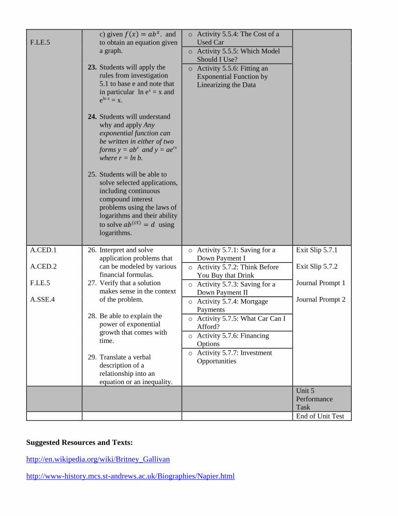
F.LE.5 c) given 𝑓(𝑥) = 𝑎𝑏𝑥. and

to obtain an equation given

a graph.

23. Students will apply the

rules from investigation

5.1 to base e and note that

in particular ln ex = x and

eln x = x.

24. Students will understand

why and apply Any

exponential function can

be written in either of two

forms y = abx and y = aerx

where r = ln b.


solve selected applications,

including continuous

compound interest

problems using the laws of

logarithms and their ability

to solve 𝑎𝑏(𝑐𝑡) = 𝑑 using

logarithms.

o Activity 5.5.4: The Cost of a

Used Car

o Activity 5.5.5: Which Model

Should I Use?

o Activity 5.5.6: Fitting an

Exponential Function by

Linearizing the Data

A.CED.1

A.CED.2

F.LE.5

A.SSE.4

26. Interpret and solve

application problems that

can be modeled by various

financial formulas.



of the problem.

28. Be able to explain the

power of exponential

growth that comes with

time.

29. Translate a verbal

description of a

relationship into an

equation or an inequality.

o Activity 5.7.1: Saving for a

Down Payment I

Exit Slip 5.7.1

Exit Slip 5.7.2

Journal Prompt 1

Journal Prompt 2

o Activity 5.7.2: Think Before

You Buy that Drink

o Activity 5.7.3: Saving for a

Down Payment II

o Activity 5.7.4: Mortgage

Payments

o Activity 5.7.5: What Car Can I

Afford?

o Activity 5.7.6: Financing

Options

o Activity 5.7.7: Investment

Opportunities

Unit 5

Performance

Task

End of Unit Test

Suggested Resources and Texts:

http://en.wikipedia.org/wiki/Britney_Gallivan

http://www-history.mcs.st-andrews.ac.uk/Biographies/Napier.html

http://en.wikipedia.org/wiki/Britney_Gallivan

http://www-history.mcs.st-andrews.ac.uk/Biographies/Napier.html

https://www.youtube.com/watch?v=KRAEbotuIE which taped the paper-folding of a piece the size of

a football field for MYTHbusters Folding Paper Seven Plus Times.

www.youtube.com/watch?v=b-MZumdfbt8

http://www-history.mcs.st-and.ac.uk/PrintHT/e.html

June 2015 Smithsonian Magazine ,”Aftershock”, pages 36 – 43 by Elizabeth Kolbert

Suggested Technology: Calculator, internet access, graphing software

https://www.youtube.com/watch?v=KRAEbotuIE

http://www.youtube.com/wartch?v=b-MZumdfbt8

http://www-history.mcs.st-and.ac.uk/PrintHT/e.html

Unit 6: Sequences and Series

Introduction and Established Goals: This chapter builds on skills from Algebra 1, where arithmetic

and geometric sequences were first introduced. The first three lessons review and extend work students

have previously done. New in this chapter is the skill of adding terms of a sequence. Partial sums and

sums of infinite geometric series are explored numerically and graphically. The final lesion in the chapter

involves recursively defined functions. This reviews knowledge of arithmetic and geometric sequences.

Connections to linear and exponential functions are made.

Desired Outcome(s):

Differentiate between an arithmetic and geometric sequence

Use explicit and recursive rules to find the nth term of a sequence

Find partial sums of sequences

Find sums of infinite geometric sequences


F-IF.A.3 Recognize that sequences are functions, sometimes defined recursively, whose domain

is a subset of the integers. For example, the Fibonacci sequence is defined recursively by

f(0) = f(1) = 1, f(n+1) = f(n) + f(n-1) for n ≥ 1.

F-BF.A.2 Write arithmetic and geometric sequences both recursively and with an explicit formula,

use them to model situations, and translate between the two forms.

F-LE.A.2 Construct linear and exponential functions, including arithmetic and geometric

sequences, given a graph, a description of a relationship, or two input-output pairs

(include reading these from a table).

A-SSE.B.4 Derive the formula for the sum of a finite geometric series (when the common ratio

is not 1), and use the formula to solve problems. For example, calculate mortgage

payments.

F-BF.A.1a Determine an explicit expression, a recursive process, or steps for calculation from a

context. SL.9-10.1.c Propel conversations by posing and responding to questions that relate the current




MP2: Use numbers to help solve problems

MP8: Use mathematical patterns to help me solve a problem


How can you write a rule for the nth term of a sequence?

How can you recognize an arithmetic sequence from its graph?

How can you recognize a geometric sequence from its graph?

How can you find the sum of an infinite geometric series?

How can you define a sequence recursively?

Key Terms/Concepts: Sequence, Terms of a sequence, Series, Summation notation, Sigma notation,

Domain, Range, Arithmetic sequence, Common difference, Arithmetic series, Linear function, Mean,

Partial sum, Repeating decimal, Fraction in simplest form, Rational number, explicit rule, recursive rule



(Content and Skill)

INSTRUCTIONAL

STRATEGIES

ASSESMENT

EVIDENCE

F-IF.A.3

SL.9-10.1.c

1. Use sequence notation to write

terms of sequences

2. Write a rule for the nth term of

a sequence

3. Sum the terms of a sequence to

obtain a series and use

summation notation

o Examples 8.1 Exit Slip 8.1

Homework o Exercises 8.1

F-IF.A.3

F-BF.A.2

F-LE.A.2

SL.9-10.1.c

4. Identify arithmetic sequences

5. Write rules for arithmetic

sequences

6. Find sums of finite arithmetic

sequences

o Explorations 1 and 2 Exit Slip 8.2

Homework o Examples 8.2

o Exercises 8.2

A-SSE.B.4

F-IF.A.3

F-BF.A.2

F-LE.A.2

SL.9-10.1.c

7. Identify geometric sequences

8. Write rules for geometric

sequences

9. Find sums of finite geometric

sequences

o Explorations 1 and 2 Exit Slip 8.3


o Exercises 8.3

Section 8.1-.3

Quiz

A-SSE.B.4

SL.9-10.1.c

10. Find partial sums of infinite

geometric series

11. Find sums of infinite

geometric series

o Explorations 1, 2, and 3 Exit Slip 8.4


o Exercises 8.4

F-IF.A.3

F-BF.A.1a

F-BF.A.2

SL.9-10.1.c

12. Evaluate recursive rules for

sequences

13. Write recursive rules for

sequences

14. Translate between recursive

and explicit rules for

sequences

15. Use recursive rules to solve

real-life Problems

o Explorations 1, 2, and 3 Exit Slip 8.5


o Exercises 8.5

Chapter Review

Performance

Task

End of Unit Test

Suggested Resources and Texts: BigIdeasMath.com

Suggested Technology: Graphing calculator, Access to internet, Microsoft Excel, Projector



Algebra II - North Stonington Public Schools

Documents

Transcript of Algebra II - North Stonington Public Schools