LINEAR ALGEBRA Math 211 - Course Outline - CiteSeerX
286
Linear Algebra LINEAR ALGEBRA Math 211 Course Outline Jim Hartman Semester I, 2004 Taylor 305 The College of Wooster Ext. 2239 Wooster, OH 44691 Linear algebra is one of the most useful courses a student of science or mathematics will ever take. It is the first course where concepts are at least as important as calculations, and applications are motivating and mind opening. Applications of linear algebra to science and real life are numerous. The solutions to many problems in physics, engineering, biology, chemistry, medicine, computer graphics, image processing, economics, and sociology require tools from linear algebra. So do all main branches of modern mathematics. ● Resources ❍ David Poole, LINEAR ALGEBRA: A Modern Introduction ❍ Maple 9.5 ® will be used extensively to perform routine computations. Some homework and exam questions will be best completed using Maple. ● Policies ❍ Grades ❍ Goals ❍ Academic Integrity ● DUE DATES ❍ November 4: Draft 1 of Proof 3 ❍ November 10: Draft 1 of Research Paper ❍ November 12: Exam 2 ❍ November 17: Draft 2 of Proof 3 ❍ November 22: Draft 2 of Research Paper ❍ December 3: Final Draft Proofs 4 & 5 ❍ December 10: Final Draft Matrix Project ● Office Hours http://www.wooster.edu/math/linalg/ (1 of 3)2005/03/08 03:48:53 Þ.Ù
-
Upload
khangminh22 -
Category
Documents
-
view
2 -
download
0
Transcript of LINEAR ALGEBRA Math 211 - Course Outline - CiteSeerX

Linear Algebra
LINEAR ALGEBRAMath 211
Course Outline
Jim Hartman Semester I, 2004
Taylor 305 The College of Wooster
Ext. 2239 Wooster, OH 44691
Linear algebra is one of the most useful courses a student of science or mathematics will ever take. It is the first course where concepts are at least as important as calculations, and applications are motivating and mind opening.
Applications of linear algebra to science and real life are numerous. The solutions to many problems in physics, engineering, biology, chemistry, medicine, computer graphics, image processing, economics, and sociology require tools from linear algebra. So do all main branches of modern mathematics.
● Resources ❍ David Poole, LINEAR ALGEBRA: A Modern Introduction ❍ Maple 9.5® will be used extensively to perform routine computations. Some homework
and exam questions will be best completed using Maple. ● Policies
❍ Grades ❍ Goals ❍ Academic Integrity
● DUE DATES ❍ November 4: Draft 1 of Proof 3❍ November 10: Draft 1 of Research Paper❍ November 12: Exam 2❍ November 17: Draft 2 of Proof 3❍ November 22: Draft 2 of Research Paper❍ December 3: Final Draft Proofs 4 & 5❍ December 10: Final Draft Matrix Project
● Office Hours
http://www.wooster.edu/math/linalg/ (1 of 3)2005/03/08 03:48:53 Þ.Ù

Linear Algebra
Monday 2-4pm
Tuesday 10-11am, 2-5pm
Wednesday 2-4pm
Thursday By Appointment Only
Friday 9-10am, 2-3pm
● Tentative Lecture Schedule
● Course Notes and Materials ❍ Short History of Linear Algebra ❍ Writing Assignments ❍ "Windows" program for matrix arithmetic ❍ Sample Exams
■ Exam 1 Fall 2004 Solutions(pdf) ■ Review for Exam 1 ■ Exam 2 Fall 2004 Solutions(pdf) ■ Review for Exam 2
❍ Lecture Notes ❍ Maple Files
■ Iterative Methods for Solving Systems of Equations ■ Maple Lab#1 (PDF Version) ■ Maple Lab#2 (PDF Version) ■ Matrix Inverse Algorithm ■ Diagonalizing Matrices
❍ Maple Command Sheet ❍ Matrix Project Example ❍ Linear Transformation Movie ❍ Change of Basis ❍ Definitions ❍ Facts ❍ Iterative Methods for Finding Eigenvalues (PDF version) ❍ Fundamental Theorem of Invertible Matrices ❍ Diagonalizability of Matrices
■ A Diagonalizable Matrix■ A Nondiagonalizable Matrix
❍ Links to the Linear Algebra World ■ OnLine Linear Algebra Text by Thomas S. Shores ■ ATLAST Project ■ Linear Algebra ToolKit ■ Elements of Abstract and Linear Algebra by Edwin H. Connell
http://www.wooster.edu/math/linalg/ (2 of 3)2005/03/08 03:48:53 Þ.Ù

Linear Algebra
■ Linear Algebra by Jim Hefferon ■ Linear Algebra Lecture Notes by Keith Matthews ■ Notes on Linear Algebra by Lee Lady ■ Electronic Journal of Linear Algebra ■ Down with Determinants by Sheldon Axler ■ Linear Algebra Glossary by John Burkhardt ■ Linear Algebra Notes by Dr. Min Yan (Hong Kong University) ■ Internet Resources for Linear Algebra - Langara College ■ Companion Website to Linear Algebra with Applications by Steven Leon ■ Linear Algebra Calculator ■ Linear Algebra Print Journals
The College of Wooster Home PageMathematics and Computer
ScienceDept. Home Page
Last Updated: July 27, 2004Jim Hartman: [email protected]
http://www.wooster.edu/math/linalg/ (3 of 3)2005/03/08 03:48:53 Þ.Ù

Jim Hartman
Mathematics and Computer Science
Jim Hartman
Professor of Mathematics
330-263-2239
The College of WoosterWooster, OH 44692
SUMMER 2005
● 2005 Summer Institute for AP Calculus ❍ Description ❍ Tentative Schedule ❍ Questions
● AP Calculus Reading ❍ May 29- June 9 ❍ I can be reached through: jimcowmath
http://www.wooster.edu/math/jhartman.html (1 of 3)2005/03/08 03:50:58 Þ.Ù

Jim Hartman
2005 SPRING SEMESTER COURSES
● Math 112 - Section 2 ❍ Calculus and Analytic Geometry II❍ Calculus by James Stewart, Brooks/Cole❍ Exam 1 Review❍ Exam 1 Solutions❍ Exam 2 Review❍ Course Formulas
● Math 102 ❍ Basic Statistics❍ The Basic Practice of Statistics by David S. Moore, Freeman❍ Course Materials
● Senior Independent Study ❍ Antoney Calistes - Differential Geometry❍ Lauren Gruenebaum - Benford's Law❍ Rebecca Young - Bootstrap Methods
OFFICE HOURS
Monday Tuesday Wednesday Thursday Friday
10-12Noon3-5PM
8-9AM11-12Noon
3-4PM 4-5PM By
Appointment10-12Noon
● EDUCATION ❍ B.S. Manchester College 1975 ❍ M.S. Michigan State University 1981 (Statistics) ❍ Ph.D. Michigan State University 1981 (Mathematics)
● PUBLICATIONS ❍ Frozen in Time, APCentral, July 2004. ❍ Some Thoughts on 2003 Calculus AB Question 6, with Riddle, Larry, APCentral, June
2003. ❍ Problem #726 Solution, College Journal of Mathematics, Volume 34, No. 3, May 2003. ❍ A Terminally Discontinuous Function, College Journal of Mathematics, Volume 27,
No. 3, May 1996. ❍ Problem #E3440 Solution, American Mathematical Monthly, Volume 99, Number 10,
Dec. 1992. ❍ Functions and Maple, CASE NEWSLETTER, Number 12, Jan. 1992. ❍ On a Conjecture of Gohberg and Rodman, Journal of Linear Algebra and Its
http://www.wooster.edu/math/jhartman.html (2 of 3)2005/03/08 03:50:58 Þ.Ù

Jim Hartman
Applications, 140: 267-278 (1990). ❍ Studying Chaotic Systems Using Microcomputer Simulations and Lyapunov
Exponents, with De Souza-Machado, S., Rollins, R. and Jacobs, D.T., American Journal of Physics, 58(4),321-329 (1990).
❍ Weighted Shifts with Periodic Weight Sequences, Illinois Journal of Mathematics, Volume 27, Number 3(1983),436-448.
❍ A Hyponormal Weighted Shift Whose Spectrum is not a Spectral Set, Journal of Operator Theory, 8(1982), 401-403.
● CAREERS IN MATHEMATICS ● ACTIVITIES/ORGANIZATIONS
❍ Mathematical Association of America (MAA) ❍ American Mathematical Society ❍ Mennonite Connected Mathematicians
● INTERESTS ❍ Linear Algebra ❍ Involutions ❍ Statistics ❍ Operator Theory ❍ 3n+1 Problem
■ A bibliography● HOBBIES
❍ Basketball ❍ Photography ❍ Bicycling
● FAMILY
Last updated: 11 February 2005Jim Hartman [email protected]
http://www.wooster.edu/math/jhartman.html (3 of 3)2005/03/08 03:50:58 Þ.Ù

The College of Wooster
Campus Tour | Interactive | Wooster Webcam
“As I have gotten to know what [Wooster]
accomplishes I can testify there is no better college
in the country.” — Loren Pope, Colleges
That Change Lives
About the College
Academic Programs
Athletics
Directories
Independent Study
Libraries Monday, March 7, 2005
College meets Walton Foundation challenge, then raises $2 million more
Wooster celebrates International Women's Day with Peggy Kelsy's Afghan Women's Project
Povertyfighters Collegiate Click Drive Feb. 14-March 31; Register for free with The College of Wooster and click twice daily
» More News Today's Events
Contact WoosterSite Index · Site Map
The College of Wooster © 2005All Rights Reserved
http://www.wooster.edu/2005/03/08 03:52:00 Þ.Ù

Policies
Course Policies
● Grades ● Goals ● Academic Integrity
Grades
Grade Determination:
Your grade will be based on the total number of points you receive out of a possible total of 1000 points. The distribution of these points is given below.
● 2 Hour Exams ❍ (100 points each)
● 1 Final Exam ❍ (200 points)
● Homework ❍ (100 points total)
● Writing Assignments ❍ Definition Quizzes
■ (200 points total) ❍ Proofs
■ (120 points total)❍ Research Topic
■ (60 points) ❍ Matrix Project
■ (100 points) ❍ Informal Writings
■ (20 points total)
Missed Exams:
Make-up exams will be given only for valid and verifiable excuses. It is important to notify me before an exam that you must miss.
http://www.wooster.edu/math/linalg/policies.html (1 of 3)2005/03/08 03:52:14 Þ.Ù

Policies
Final Exam:
Section 1 -Friday, December 12, 2:00 PM
Section 2 - Thursday, December 11, 7:00 PM
Math 211 Home Page
Course Goals
● To learn about matrices and their properties. ● To learn about vector spaces and inner product spaces. ● To see different examples of these spaces. ● To learn about linear transformations on these spaces. ● To learn about applications of linear algebra. ● To learn how to construct proofs of known theorems. ● To improve mathematics writing with attention to the writing process
Math 211 Home Page
Academic Integrity
I encourage students to exchange ideas and discuss problems. However, for homework to be turned in, it will be considered plagarism if a student copies the work of another. On exams or quizzes the giving or receiving of aid is not permitted. Any violation of the Code of Academic Integrity should be reported to the instructor who will take appropriate disciplinary action and/or inform the Judicial Board of the case. In either case, the Dean's office will be notified of the violation.
Code of Academic Integrity
http://www.wooster.edu/math/linalg/policies.html (2 of 3)2005/03/08 03:52:14 Þ.Ù

Policies
Math 211 Home Page
http://www.wooster.edu/math/linalg/policies.html (3 of 3)2005/03/08 03:52:14 Þ.Ù

Lecture Schedule
TENTATIVE LECTURE SCHEDULE
DATE TOPIC DATE TOPIC
August 30 1.1 25 Quiz 6
September 1 1.2 27 5.2
2 Problems 28 Problems
3 2.1 29 5.3
6 Quiz 1 November 1 Quiz 7
8 2.2 3 5.4
9 Lab#1 4 Problems
10 2.3 5 6.1
13 Quiz 2 8 Quiz 8
15 2.5 10 6.2
16 Problems 11 Review
17 3.1 12 EXAM 2
20 Quiz 3 15 Quiz 9
22 3.2 17 6.3
23 Problems 18 Problems
24 3.3 19 6.4
27 3.4 22 Quiz 10
29 3.5 24 Break
30 Review 25 Break
October 1 EXAM 1 26 Break
4 Quiz 4 29 6.5
6 4.1 December 1 6.6
7 LAB #2 2 LAB #3
http://www.wooster.edu/math/linalg/lecture.html (1 of 2)2005/03/08 03:52:27 Þ.Ù

Lecture Schedule
8 4.2 3 7.1
11 Quiz 5 6 7.2
13 4.3 8 7.3
14 Problems 9 Problems
15 4.4 10 REVIEW
FINALS WEEK
18FALL
BREAK13
20 4.5 14 FINAL - 9am
21 Problems 15 FINAL - 7pm
22 5.1 16
Return to Math 211 Home Page
http://www.wooster.edu/math/linalg/lecture.html (2 of 2)2005/03/08 03:52:27 Þ.Ù

History
A Brief History of Linear Algebra
There would be many things to say about this theory of matrices which should, it seems to me, precede the theory of determinants. Arthur Cayley, 1855
Determinants Used Before Matrices
● 1693 Leibniz ● 1750 Cramer
❍ solving systems of equations
Implicit Use of Matrices
● Late 18th century ● Lagrange
❍ bilinear forms for the optimization of a real valued function of 2 or more variables
Gaussian Elimination
● 1800 Gauss ❍ Method known by Chinese for 3x3 in 3rd century BC
Vector Algebra
● 1844 Grassmann
http://www.wooster.edu/math/linalg/history.html (1 of 3)2005/03/08 03:52:33 Þ.Ù
History
Matrix Algebra
● 1848 J. J. Sylvester ❍ introduced the term matrix which is the Latin word for womb (determinants emanate from
a matrix) ❍ define the nullity of a matrix in 1884
● 1855 Arthur Cayley ❍ definition of matrix multiplication motivated by composite transformations, also
introduced inverses ● 1878 George Frobenius
❍ introduced rank and proved the Cayley-Hamilton Theorem
Vector Space
● 1888 Peano ❍ modern definition of vector space
Further Developments
● 1942 J. Willard Gibbs ❍ further development of ideas by this mathematical physicist
● 1942 John von Neumann ❍ condition number
● 1948 Alan Turing ❍ LU decomposition
● 1958 J. H. Wilkinson ❍ QR factorization
Linear Algebra in the Curriculum
● 1941 Birkhoff and MacLane ❍ appearance in the basic graduate text Modern Algebra
● 1959 Kemeny, Snell, Thompson, & Mirkel ❍ appearance in the undergraduate text Finite Mathematical Structures
● 1960 Widespread adoption into lower division mathematics curriculum
http://www.wooster.edu/math/linalg/history.html (2 of 3)2005/03/08 03:52:33 Þ.Ù

History
● 1965 CUPM Recommendations ❍ suggest linear algebra be a course in the undergraduate curriculum and content for the
course ● 1990 New CUPM Guidelines look at the focus of the linear algebra course ● 1990's Experimentation with technology and content
Math 211 Home Page
http://www.wooster.edu/math/linalg/history.html (3 of 3)2005/03/08 03:52:33 Þ.Ù

Writing
WRITING ASSIGNMENTS
DEFINITION QUIZZESPROOFSMATRIX PROJECTRESEARCH TOPICINFORMAL WRITINGS
Math 211 Home Page
DEFINITION QUIZZES
VALUE: 200 points total
Quizzes will be given almost every Monday of the semester during the first 10-15 minutes of class. These quizzes will only ask you to state definitions of terms used. Those definitions will come from the material studied in the previous class periods that have not been previously quizzed. There are more definitions than those simply labeled with the word "definition" in the book. Terms not appearing in the book, but given in class, might also be tested.
TO TOP
PROOFS
DUE DATES: To be determinedVALUE: 120 points total (30 points each)
You are asked to submit proofs of the following theorems. These proofs will, after revision, be clear, complete, and accurate. These are theorems that might be referred to in class, but will not be proved. The proofs should be written with the audience being your fellow classmates.
Theorem 1: For vectors u and v in ℜn, ||u + v|| ≤ ||u|| + ||v||.
http://www.wooster.edu/math/linalg/writeassign.html (1 of 3)2005/03/08 03:52:45 Þ.Ù

Writing
Theorem 2:The vectors v1,v2, . . . ,vn are linearly independent. If w is not in span(v1,v2, . . . ,vn) then w,v1,v2, . . . ,
vn are linearly independent.
Theorem 3:
Theorem 4:
TO TOP
MATRIX PROJECT
First Draft Due: November 2004Final Draft Due: December 10, 2004
VALUE: 100 points
You will be given three matrices. Your assignment is to describe anything about these matrices that you can. Some of the ideas that you should explore as you work with these matrices are:1) Examine any interesting arithmetic properties 2) Examine what happens when I "combine" this matrix with others 3) Examine whether this matrix fits into a more general class of matrices. If so,find the properties of that class. Determine whether that class is a subspaceof all matrices of the appropriate "size." 4) Find characteristics about the matrix that we have studied in class, such as determinant, row space, column space, null space, rank, eigenvalues and eigenvectors. An example of the kind of work I would like to see can be obtained from me personally, or retrieved from the course website. Your paper should be written as if it was going to be read by your fellow students. Thus you should assume they have the basic knowledge from this course, but nothing beyond. One goal of this assignment is to show that you understand the concepts that have been covered in this course. A second goal is for you to begin to explore properties and structures that you may not have encountered before and to begin to ask your own questions about what you are encountering. This is a creative exercise and you may do anything (legal) to these matrices that you desire. Use your imagination.
Your final paper should be completed in Word® or Maple®. It should be double-spaced and be of a length that is sufficient to describe the properties of each matrix. If you get help from other sources, they
http://www.wooster.edu/math/linalg/writeassign.html (2 of 3)2005/03/08 03:52:45 Þ.Ù

Writing
need to be cited and referenced. You are free to determine the organization of your paper, but should express your ideas in clear and concise ways with flawless grammar and spelling. This is both a writing assignment and a mathematics assignment. You are writing about mathematics that you are exploring. I will read and comment on the first draft. You will then be able to make revisions based upon my comments. The grade for the paper will be based upon the final draft, although I will give you a preliminary grade based upon your first draft to give you an idea of where you stand.
The paper will be graded based upon a primary trait analysis which will be provided later.
TO TOP
RESEARCH TOPIC
DUE DATE: First part of the semesterVALUE: 60 points
During the first part of the semester, I will ask you to research some topic in linear algebra. This topic will either be chosen from a list or be an approved topic of your own choice. You will need to provide a bibliography with this paper along with inline citations.
TO TOP
INFORMAL WRITINGS
DUE DATE: December 10, 2004VALUE: 20 points
Throughout the semester, I will ask you to complete writings both in and out of class. Some of these may be freewrites, while others I will ask you to construct more carefully or on a particular subject. Some will be submitted in class; others will be submitted by email. The points given here will be primarily for the completion of and effort given to these writing tasks rather than the quality of the writing.
TO TOP
http://www.wooster.edu/math/linalg/writeassign.html (3 of 3)2005/03/08 03:52:45 Þ.Ù

Matrix Calculator
Search: Angelfire Web by
Build an Online Photo Album Try Blogging for FREE
Matrix Calculator - NEW VERSION AVAILABLE!
Mcalcdos is a free command line linear algebra calculator capable of matrix, vector and polynomial operations in real and complex fields.
Download
Download mcalcdos.exe v0.3 for free!!
A newly updated version of mcalcdos.exe is now available! Please click above to download the latest version, which includes an up-to-date help file.
Click here for updates made to the current release.
To use, simply input mathematical expressions in the same manner as written to return the result. For a list of available functions, type help. To ease input, multiplication is implied between adjacent operands.
e^(2 pi i) + 0.5 cos (2 pi/3)
http://www.angelfire.com/space/matrixcalc/ (1 of 2)2005/03/08 03:54:11 Þ.Ù

Matrix Calculator
Variables are assigned using = as in the following example:
a = (1 + sqrt 5) / 2
Once assigned, variables can be used in subsequent expressions. The variable ans is automatically updated to the result of the previous expression. Other reserved names include pi, i, e, X (which is used in polynomial expressions) and all the function names. Any other variable names are permitted.
varname = 14 e ^ 0.7
newvar = 3.7! + varname
Input matrices with [], vectors with {} and polynomials with X
matrix_A = [4, 7][2, 3]
vector_b = {1, -2}
inverse a * b
eval (X^3 - 7X + 1, -3)
Eventually, this program will be given a windows GUI, but until then, feel free to use and distribute the text based version. Please contact me with any questions, comments or for (very) limited support.
Email: [email protected]
OR
http://www.angelfire.com/space/matrixcalc/ (2 of 2)2005/03/08 03:54:11 Þ.Ù

1
MATH 211 TEST I
Name SOLUTIONS Fall 2004 PLEASE SHOW ALL OF YOUR WORK!! 1.(15 PTS) Consider the system of equations given by Ax=b, and let C = [A | b] be the
augmented matrix for that system. If G=[M | d] is the reduced, row-echelon form of C:
a) What will you see in G if the system is inconsistent? b) What will you see in G if the system has exactly one solution? c) What will you see in G if this system has infinitely many solutions? a) There will be a leading 1 in the last column of G, i.e. in d. b) There will be a leading 1 in every column of M and not in d. c) There will be a column of M without a leading 1 and d will not have a
leading 1. 2.(10 PTS) Suppose we have the system of equations given by Ax=b. Let x1 be a particular
solution to this equation. Show that if x2 is any other solution to this system then x2 - x1 is a solution to the homogeneous system Ax=0.
A(x2 – x1) = Ax2 – A x1 = b – b = 0. 3.(10 PTS) Through two examples illustrate how matrix multiplication does not satisfy two
distinct properties that real number multiplication does. Consider the following two examples.
!
1 1
1 1
"
# $
%
& '
2 2
-2 -2
"
# $
%
& ' =
0 0
0 0
"
# $
%
& ' and
!
2 2
"2 "2
# $ %
& ' ( 1 1
1 1
# $ %
& ' ( =
4 4
-4 -4
# $ %
& ' (
These two equations show two things. First, matrix multiplication is not commutative. Second, the product of two nonzero matrices can be zero.
4.(10 PTS)
!
M =
2 5 6 "5 0
2 2 "6 "5 "3
3 3 "9 "2 1
#
$
% % %
&
'
( ( (
has
!
rref M( ) =
1 0 "7 0 0
0 1 4 0 1
0 0 0 1 1
#
$
% % %
&
'
( ( (
.
a) Express any columns of M, that are possible, as linear combinations of other columns of M. Let m1, m2, m3, m4, m5 be the columns of M. Then m3 = -7m1 + 4m2 and m5 = m2 + m4.

2
b) Find a spanning set for the homogeneous system of linear equations given by Mx = 0.
The solutions to Mx = 0 are given by x1 = 7x3, x2 = -4x3 – x5 and x4 = -x5.
This leads to a solution vector of
!
7x3
"4x3" x
5
x3
"x5
x5
#
$
% % % % % %
&
'
( ( ( ( ( (
= x3
7
"4
1
0
0
#
$
% % % % % %
&
'
( ( ( ( ( (
+ x5
0
"1
0
"1
1
#
$
% % % % % %
&
'
( ( ( ( ( (
. Thus a spanning set is
!
7
"4
1
0
0
#
$
% % % % % %
&
'
( ( ( ( ( (
,
0
"1
0
"1
1
#
$
% % % % % %
&
'
( ( ( ( ( (
)
*
+ + +
,
+ + +
-
.
+ + +
/
+ + +
.
5.(10 PTS) Suppose u, v, and w are nonzero orthogonal vectors.
a) Show that ||u + v + w||2 = ||u||2 + ||v||2 + ||w||2. ||u + v + w||2 = (u + v + w)•( u + v + w) = u•u + u•v + u•w + v•u + v•v + v•w + w•u + w•v + w•w = ||u||2 + 0 + 0 + 0 + ||v||2 + 0 + 0 + 0 + ||w||2 = ||u||2 + ||v||2 + ||w||2 b) Show that u, v, w are linearly independent.
If αu + βv + γw = 0 then u•(αu + βv + γw) = u•0 = 0 so αu•u + βu•v + γu•w = 0 or α||u||2 + β(0) + γ(0) = 0 or α||u||2 = 0. Since ||u||2 ≠ 0 we must have α = 0. Similarly be considering v•(αu + βv + γw) = v•0 = 0 and w•(αu + βv + γw) = w•0 = 0 we also get β = γ = 0. Since we have α = β = γ = 0, the vectors u, v, and w are linearly independent. 6.(10 PTS) Suppose u, v, and w are linearly independent vectors. Show that u + v + w, v + w, v – w are linearly independent. If α( u + v + w) + β(v + w) + γ(v - w)w = 0 then αu + (β+γ)v + (β-γ)w = 0. Since u, v, and w are linearly independent we must have α = 0, β+γ = 0 and β-γ = 0. The
last two equations imply that β = γ = 0. Combining this with α = 0 says the vectors are linearly independent.

3
7.(10 PTS) A vector y in ℜm is said to be the in the range of the matrix A if there is a
vector x in ℜn such that y = Ax. a) Show that if y1 and y2 are in the range of A then so is y1 + y2.
y1 = Ax1 and y2 = Ax2 so that y1 + y2 = Ax1 + Ax2 = A(x1 + x2) so y1+y2 is in the range of A.
b) Show that if α is a scalar and y is in the range of A then αy is in the range of A. αy = αAx = A(αx) so αy is in the range of A also.

4
MATH 211
TEST I TAKE HOME PROBLEMS
Name Solutions for this part are attached. Fall 2004
Note: If you use MAPLE on these problems, please provide me with a printed copy of all the work you did. You can label that printout or add to it to indicate answers to questions. DUE DATE: Wednesday, 6 October 2004 - 4:00 PM (EDT)
8.( 10 PTS) Consider the list of vectors
!
8
4
"5
"5
3
#
$
% % % % % %
&
'
( ( ( ( ( (
,
1
0
0
0
0
#
$
% % % % % %
&
'
( ( ( ( ( (
,
"5
8
5
"1
0
#
$
% % % % % %
&
'
( ( ( ( ( (
.
a) Show that the 3 vectors above are linearly independent. b) Find two more vectors in ℜ5 so that the span of the 5 vectors is ℜ5. Indicate how you know that your 5 vectors span ℜ5. 9.(15 PTS) An mxn matrix A is said to have a left inverse if there is an nxm matrix B so that BA = Im.
a) Find a left inverse for the matrix
!
M =
8 1 "5
4 0 8
"5 0 5
"5 0 "1
3 0 0
#
$
% % % % % %
&
'
( ( ( ( ( (
.
b) Does M have only one left inverse? Don't just answer yes or no to this question. If there is more than one, find a second one. If there is exactly one, prove it. Just how many left inverses, does M have.
c) What conditions must be placed upon an mxn matrix M to guarantee that it has a left inverse?
d) A matrix A is said to have a right inverse if there is a matrix B so that AB=I.
Show that the matrix M above cannot have a right inverse.

Linear AlgebraExam 1 Maple Solutions
> with(LinearAlgebra):
Problem 8> v1:=<8,4,-5,-5,3>:v2:=<1,0,0,0,0>:v3:=<-5,8,5,-1,0>:
Part a)> M:=<v1|v2|v3>;
M :=
8 1 -5
4 0 8
-5 0 5
-5 0 -1
3 0 0
éêêêêêêêêêë
ùúúúúúúúúúû
> ReducedRowEchelonForm(M);1 0 0
0 1 0
0 0 1
0 0 0
0 0 0
éêêêêêêêêêë
ùúúúúúúúúúû
Since there is a leading 1 in every column of rref(M), the columns of M are linearly independent.
Part b)> N:=<M|IdentityMatrix(5)>;
N :=
8 1 -5 1 0 0 0 0
4 0 8 0 1 0 0 0
-5 0 5 0 0 1 0 0
-5 0 -1 0 0 0 1 0
3 0 0 0 0 0 0 1
éêêêêêêêêêë
ùúúúúúúúúúû
> ReducedRowEchelonForm(N);

1 0 0 0 0 0 0 13
0 1 0 1 0 0 -5 -11
0 0 1 0 0 0 -1 -53
0 0 0 0 1 0 8 12
0 0 0 0 0 1 5 10
éêêêêêêêêêêêêêë
ùúúúúúúúúúúúúúû
This matrix has leading 1's in columns 1,2,3,5,6 and indicates that the corresponding 5 columns of N are linearly independent and should span R^5. One can see this from the following three Maple commands.
> v4:=SubMatrix(N,1..5,5):v5:=SubMatrix(N,1..5,6):
> V:=<v1|v2|v3|v4|v5|<x,y,z,w,e>>;
V :=
8 1 -5 0 0 x
4 0 8 1 0 y
-5 0 5 0 1 z
-5 0 -1 0 0 w
3 0 0 0 0 e
éêêêêêêêêêë
ùúúúúúúúúúû
> ReducedRowEchelonForm(V);
1 0 0 0 0 13
e
0 1 0 0 0 x - 5 w - 11 e
0 0 1 0 0 - 53
e - w
0 0 0 1 0 8 w + y + 12 e
0 0 0 0 1 10 e + z + 5 w
éêêêêêêêêêêêêêë
ùúúúúúúúúúúúúúû
This last matrix shows that any vector <x,y,z,w,e> in R 5 can be written as a linear combination of the first 5 columns of V. Thus the set
> {v1,v2,v3,v4,v5};

8
4
-5
-5
3
éêêêêêêêêêë
ùúúúúúúúúúû
,
-5
8
5
-1
0
éêêêêêêêêêë
ùúúúúúúúúúû
,
1
0
0
0
0
éêêêêêêêêêë
ùúúúúúúúúúû
,
0
1
0
0
0
éêêêêêêêêêë
ùúúúúúúúúúû
,
0
0
1
0
0
éêêêêêêêêêë
ùúúúúúúúúúû
ìïïïïïíïïïïïî
üïïïïïýïïïïïþ
is a basis for R 5.
Problem 9
Part a)> C:=<v1|v2|v3|v4|v5>;
C :=
8 1 -5 0 0
4 0 8 1 0
-5 0 5 0 1
-5 0 -1 0 0
3 0 0 0 0
éêêêêêêêêêë
ùúúúúúúúúúû
> X:=C^(-1);
X :=
0 0 0 0 13
1 0 0 -5 -11
0 0 0 -1 -53
0 1 0 8 12
0 0 1 5 10
éêêêêêêêêêêêêêë
ùúúúúúúúúúúúúúû
> A:=SubMatrix(X,1..3,1..5);
A :=
0 0 0 0 13
1 0 0 -5 -11
0 0 0 -1 -53
éêêêêêêêêë
ùúúúúúúúúû
> A.M;

1 0 0
0 1 0
0 0 1
éêêêêë
ùúúúúû
Thus the matrix A above is a left inverse for M.
Part b)There are infinitely many left inverses for M. Consider the following computations.
> A1:=<<x1,x2,x3>|<x4,x5,x6>|<x7,x8,x9>|<x10,x11,x12>|<x13,x14,x15>>;
A1 :=
x1 x4 x7 x10 x13
x2 x5 x8 x11 x14
x3 x6 x9 x12 x15
éêêêêë
ùúúúúû
> H:=A1.M;
H :=
8 x1 + 4 x4 - 5 x7 - 5 x10 + 3 x13 x1 -5 x1 + 8 x4 + 5 x7 - x10
8 x2 + 4 x5 - 5 x8 - 5 x11 + 3 x14 x2 -5 x2 + 8 x5 + 5 x8 - x11
8 x3 + 4 x6 - 5 x9 - 5 x12 + 3 x15 x3 -5 x3 + 8 x6 + 5 x9 - x12
éêêêêë
ùúúúúû
> sol:=solve({H[1,1]=1,H[1,2]=0,H[1,3]=0,H[2,1]=0,H[2,2]=1,H[2,3]=0,H[3,1]=0,H[3,2]=0,H[3,3]=1});
sol := ìíîx15 = 12 x6 + 10 x9 - 5
3, x10 = 8 x4 + 5 x7, x1 = 0, x2 = 1, x3 = 0, x11 = -5 + 8 x5 + 5 x8,
x12 = -1 + 8 x6 + 5 x9, x14 = -11 + 12 x5 + 10 x8, x13 = 13
+ 12 x4 + 10 x7, x4 = x4, x5 = x5,
x6 = x6, x7 = x7, x8 = x8, x9 = x9üýþ
> assign(sol);
> A1;A1.M;
0 x4 x7 8 x4 + 5 x7 13
+ 12 x4 + 10 x7
1 x5 x8 -5 + 8 x5 + 5 x8 -11 + 12 x5 + 10 x8
0 x6 x9 -1 + 8 x6 + 5 x9 12 x6 + 10 x9 - 53
éêêêêêêêêë
ùúúúúúúúúû
1 0 0
0 1 0
0 0 1
éêêêêë
ùúúúúû

Every matrix of the form of A1 above is a left inverse for M as indicated by the computation above. There are infinitely many since the free variables x4,x5,x6,x7,x8,x9 can be chosen to be any real numbers. If we let them all be zero then
> x4:=0:x5:=0:x6:=0:x7:=0:x8:=0:x9:=0:A1;
0 0 0 0 13
1 0 0 -5 -11
0 0 0 -1 -53
éêêêêêêêêë
ùúúúúúúúúû
the matrix above is a particular second left inverse for M.
Part c)The columns of M must be linearly independent in order for M to have a left inverse. This can be seen in a couple of ways. One way uses the idea I used to construct the first left inverse of M. If the columns of M are linearly independent, one can add two other columns to get an invertible matrix. This matrix will yield a left inverse by taking the upper 3x5 submatrix of the inverse. If the columns are not linearly independent this process is not possible. moreover if A is a left inverse and Mx=0 then x = Ix = AMx = A0 = 0 and hence the columns of M are linearly independent. These two parts together show M has a leftinverse iff the columns of M are linearly independent.
Part d)If M had a right inverse then every vector in R5 could be written as a linear combination of the columns of M. But we already know the vector <0,1,0,0,0> cannot be written as a linear combination of the columns of M. This was seen in part a) but can also been seen in:
> N:=<M|<0,1,0,0,0>>;
N :=
8 1 -5 0
4 0 8 1
-5 0 5 0
-5 0 -1 0
3 0 0 0
éêêêêêêêêêë
ùúúúúúúúúúû
> ReducedRowEchelonForm(N);1 0 0 0
0 1 0 0
0 0 1 0
0 0 0 1
0 0 0 0
éêêêêêêêêêë
ùúúúúúúúúúû

The leading 1 in the last column verifies the statement above.

Review 1
Math 211 Linear AlgebraExam 1
Fundamental Ideas
A. Systems of Equations
1. Augmented Matrix2. RREF3. Ax = b
B. Vectors
1. Addition and Scalar Multiplication2. Dot Product , Norm, and Orthogonality3. Orthogonal Projection
C. Matrices
1. Addition, Scalar Multiplication, and Multiplication2. Inverses3. Transpose4. Elementary Matrices5. Rank6. RREF
D. Span and Linear Combinations
E. Linear Independence
http://www.wooster.edu/math/linalg/review1.html2005/03/08 03:57:36 Þ.Ù

1
MATH 211
EXAM 2 Name Fall 2004 PLEASE SHOW ALL OF YOUR WORK!!
1.(10 PTS) Find a basis for the subspace of ℜ4 given by
!
x " 2y
2y " x
x " 2y + z
z
#
$
% % % %
&
'
( ( ( (
: x,y,x ) *
+
,
- -
.
- -
/
0
- -
1
- -
. What is the
dimension of this subspace? SOLUTION
!
x " 2y
2y " x
x " 2y + z
z
#
$
% % % %
&
'
( ( ( (
= x
1
"1
1
0
#
$
% % % %
&
'
( ( ( (
+ y
"2
2
"2
0
#
$
% % % %
&
'
( ( ( (
+ z
0
0
1
1
#
$
% % % %
&
'
( ( ( (
= x " 2y( )
1
"1
1
0
#
$
% % % %
&
'
( ( ( (
+ z
0
0
1
1
#
$
% % % %
&
'
( ( ( (
. Thus a basis for the subspace is
!
1
"1
1
0
#
$
% % % %
&
'
( ( ( (
,
0
0
1
1
#
$
% % % %
&
'
( ( ( (
)
*
+ +
,
+ +
-
.
+ +
/
+ +
and its dimension is 2.
2.(18 PTS) For
!
A =
8 "5 31 "2 3
4 8 "16 20 "4
"5 5 "25 5 "5
"5 "1 "7 "7 "2
3 0 6 3 "1
#
$
% % % % % %
&
'
( ( ( ( ( (
,
!
rref (A) =
1 0 2 1 0
0 1 "3 2 0
0 0 0 0 1
0 0 0 0 0
0 0 0 0 0
#
$
% % % % % %
&
'
( ( ( ( ( (
.
a) Give a basis for col(A).
SOLUTION
!
8
4
"5
"5
3
#
$
% % % % % %
&
'
( ( ( ( ( (
,
"5
8
5
"1
0
#
$
% % % % % %
&
'
( ( ( ( ( (
,
3
"4
"5
"2
"1
#
$
% % % % % %
&
'
( ( ( ( ( (
)
*
+ + +
,
+ + +
-
.
+ + +
/
+ + +
is a basis for col(A).
b) Give a basis for row( )A .
SOLUTION
!
1 0 2 1 0[ ], 0 1 "3 2 0[ ], 0 0 0 0 1[ ]{ } is a basis for the row space.

2
c) Give a basis for null(A). SOLUTION
A vector
!
x1
x2
x3
x4
x5
"
#
$ $ $ $ $ $
%
&
' ' ' ' ' '
will be in the nullspace if and only if x1 + 2x3 + x4 = 0, x2 – 3x3 + 2x4 = 0,
and x5 = 0. This implies
!
x1
x2
x3
x4
x5
"
#
$ $ $ $ $ $
%
&
' ' ' ' ' '
=
(2x3( x
4
3x3( 2x
4
x3
x4
0
"
#
$ $ $ $ $ $
%
&
' ' ' ' ' '
= x3
(2
3
1
0
0
"
#
$ $ $ $ $ $
%
&
' ' ' ' ' '
+ x4
(1
(2
0
1
0
"
#
$ $ $ $ $ $
%
&
' ' ' ' ' '
. Thus
!
"2
3
1
0
0
#
$
% % % % % %
&
'
( ( ( ( ( (
,
"1
"2
0
1
0
#
$
% % % % % %
&
'
( ( ( ( ( (
)
*
+ + +
,
+ + +
-
.
+ + +
/
+ + +
is a basis
for null(A).
c) What is rank(A)? SOLUTION rank(A) = 3
d) What is nullity(A)? SOLUTION nullity(A) = 3 f) Is A invertible? Why or why not? SOLUTION A is not invertible because rank(A) = 3 < 5. To be invertible, its rank would have to be 5.
3.(10 PTS) The columns of
!
B =
12
12
12
12
12
" 12
12
" 12
12
12
" 12
" 12
12
" 12
" 12
12
#
$
% % % % %
&
'
( ( ( ( (
form an orthonormal basis for ℜ4.

3
a) Write the vector
!
1
2
3
4
"
#
$ $ $ $
%
&
' ' ' '
as a linear combination of the columns of B.
SOLUTION
!
1
2
3
4
"
#
$ $ $ $
%
&
' ' ' '
=
1
2
3
4
"
#
$ $ $ $
%
&
' ' ' '
•
12
12
12
12
"
#
$ $ $ $ $
%
&
' ' ' ' '
(
)
* * * * *
+
,
- - - - -
12
12
12
12
"
#
$ $ $ $ $
%
&
' ' ' ' '
+
1
2
3
4
"
#
$ $ $ $
%
&
' ' ' '
•
12
. 12
12
. 12
"
#
$ $ $ $ $
%
&
' ' ' ' '
(
)
* * * * *
+
,
- - - - -
12
. 12
12
. 12
"
#
$ $ $ $ $
%
&
' ' ' ' '
+
1
2
3
4
"
#
$ $ $ $
%
&
' ' ' '
•
12
12
. 12
. 12
"
#
$ $ $ $ $
%
&
' ' ' ' '
(
)
* * * * *
+
,
- - - - -
12
12
. 12
. 12
"
#
$ $ $ $ $
%
&
' ' ' ' '
+
1
2
3
4
"
#
$ $ $ $
%
&
' ' ' '
•
12
. 12
. 12
12
"
#
$ $ $ $ $
%
&
' ' ' ' '
(
)
* * * * *
+
,
- - - - -
12
. 12
. 12
12
"
#
$ $ $ $ $
%
&
' ' ' ' '
= 5( )
12
12
12
12
"
#
$ $ $ $ $
%
&
' ' ' ' '
+ .1( )
12
. 12
12
. 12
"
#
$ $ $ $ $
%
&
' ' ' ' '
+ .2( )
12
12
. 12
. 12
"
#
$ $ $ $ $
%
&
' ' ' ' '
+ 0( )
12
. 12
. 12
12
"
#
$ $ $ $ $
%
&
' ' ' ' '
b) What is B-1?
SOLUTION
!
B"1
= BT
=
12
12
12
12
12
" 12
12
" 12
12
12
" 12
" 12
12
" 12
" 12
12
#
$
% % % % %
&
'
( ( ( ( (
= B
4.(12 PTS) Consider the matrix
!
B ="1 9
6 "4
#
$ %
&
' ( .
a) Find eigenvalues and corresponding eigenvectors for B. SOLUTION
!
"I # B =" +1 #9
#6 " + 4
$
% &
'
( ) and det(λI-B) = (λ+1)(λ+4) – 54 = λ2 + 5λ - 50 = (λ + 10)(λ - 5).
Thus B has two eigenvalues -10 and 5.
For λ = 5 we need null(5I – B) =
!
null6 "9
"6 9
#
$ %
&
' (
)
* +
,
- . = span
3
2
#
$ % &
' (
)
* +
,
- . and for λ = -10 we need
null(-10I – B) =
!
null"9 "9
"6 "6
#
$ %
&
' (
)
* +
,
- . = span
"1
1
#
$ %
&
' (
)
* +
,
- . . The vectors that span those nullspaces are
eigenvectors corresponding to the eigenvalues.

4
b) Describe the eigenspaces for each of the eigenvalues.
SOLUTION
The two eigenspaces are
!
E5
= span3
2
"
# $ %
& '
(
) *
+
, - and
!
E"10 = span"1
1
#
$ %
&
' (
)
* +
,
- . .
c) Give the algebraic and geometric multiplicities of each of the eigenvalues.
SOLUTION The algebraic and geometric multiplicity of each eigenvalue is 1. 5.(10 PTS) Let M be a 3x5 matrix with rank(M)=3. Fill in the following blanks.
a) The columns of M are linearly dependent . (independent or dependent) b) The rows of M are linearly independent . (independent or dependent) c) nullity(M) = 2 d) rank(MT) = 3
e) nullity(MT) = 0
6.(10 PTS) Let T:ℜ2 → ℜ3 be given by
!
Tx
y
"
# $ %
& '
(
) *
+
, - =
2y . x
x . 3y
y 2
"
#
$ $ $
%
&
' ' '
.
a) Show that T is a linear transformation.
SOLUTION
!
Tx
y
"
# $ %
& '
(
) *
+
, - =
2y . x
x . 3y
y 2
"
#
$ $ $
%
&
' ' '
=
.1 2
1 .3
0 2
"
#
$ $ $
%
&
' ' ' x
y
"
# $ %
& ' . This implies T is a matrix transformation and hence is
a linear transformation.
b) Find the matrix of T with respect to the standard basis. SOLUTION
The matrix of T is
!
"1 2
1 "3
0 2
#
$
% % %
&
'
( ( ( .

5
7,(5 PTS) Let A and B be matrices with C = AB. Show that null(B) ⊂ null(C). What does this say about rank(C) in comparison to rank(B)? SOLUTION If x ∈ null(B) then Bx = 0. So Cx = ABx = A0 or (AB)x = 0. Thus x ∈ null(C). This says null(B) ⊂ null(C). Since nullity(B) ≤ nullity(C) and B and C have the same number of columns, we must have rank(C) ≤ rank(B) since B and C have the same number of columns and rank(M) + nullity(M) = the number of columns of M for any matrix M.
MATH 211 EXAM 2
TAKE HOME PROBLEMS
Name SOLUTIONS Fall 2004
Note: If you use MAPLE on these problems, please provide me with a printed copy of all the work you did. You can label that printout or add to it to indicate answers to questions. DUE DATE: Wednesday, 13 November 2004 - 4:00 PM (EST)
THE SOLUTIONS TO THIS PART ARE FOUND BELOW!
8.(16 PTS) Consider the matrix
!
A =
9 "17 1 15
"15 7 17 "1
1 15 9 "17
17 "1 "15 7
#
$
% % % %
&
'
( ( ( (
.
a) Find all eigenvalues for A.
b) Determine the algebraic multiplicity of each of the eigenvalues for A.
c) Find bases for each of the eigenspaces for A.
d) Determine the geometric multiplicity of each of the eigenvalues for A.
9.(9 PTS) Let
!
B =
5 "8 0 1 8
"7 4 0 9 0
0 0 4 0 0
1 8 0 5 "8
9 0 0 "7 4
#
$
% % % % % %
&
'
( ( ( ( ( (
. Show how to diagonalize B.

EXAM 2TAKE HOME SOLUTIONS
FALL 2004> with(LinearAlgebra):
Problem 8> A:=<<9,-15,1,17>|<-17,7,15,-1>|<1,17,9,-15>|<15,-1,-17,7>>;
A :=
9 -17 1 15
-15 7 17 -1
1 15 9 -17
17 -1 -15 7
éêêêêêêêë
ùúúúúúúúû
Part a)> ei:=Eigenvectors(A,output=list);
ei := -24, 1,
-1
-1
1
1
éêêêêêêêë
ùúúúúúúúû
ìïïïíïïïî
üïïïýïïïþ
éêêêêêêêêë
ùúúúúúúúúû
, 40, 1,
1
-1
-1
1
éêêêêêêêë
ùúúúúúúúû
ìïïïíïïïî
üïïïýïïïþ
éêêêêêêêêë
ùúúúúúúúúû
, 8, 2,
1
1
1
1
éêêêêêêêë
ùúúúúúúúû
ìïïïíïïïî
üïïïýïïïþ
éêêêêêêêêë
ùúúúúúúúúû
éêêêêêêêêë
ùúúúúúúúúû
A has 3 eigenvalues. They are -24, 40, and 8.
Part b)The algebraic multiplicity of -24 is 1. The algebraic multiplicity of 40 is 1. The algebraic multiplicity of 8is 2.
Part c)A basis for E-24 is:
> ei[1][3];-1
-1
1
1
éêêêêêêêë
ùúúúúúúúû
ìïïïíïïïî
üïïïýïïïþ

A basis for E40 is:
> ei[2][3];1
-1
-1
1
éêêêêêêêë
ùúúúúúúúû
ìïïïíïïïî
üïïïýïïïþ
A basis for E8 is:
> ei[3][3];1
1
1
1
éêêêêêêêë
ùúúúúúúúû
ìïïïíïïïî
üïïïýïïïþ
Part d)The geometric multiplicity of each of the three eigenvalues is 1.
Problem 9> B:=<<5,-7,0,1,9>|<-8,4,0,8,0>|<0,0,4,0,0>|<1,9,0,5,-7>|<8,0,0,-8,4>>;
B :=
5 -8 0 1 8
-7 4 0 9 0
0 0 4 0 0
1 8 0 5 -8
9 0 0 -7 4
éêêêêêêêêêë
ùúúúúúúúúúû
> eib:=Eigenvectors(B,output=list);
eib := -12, 1,
-1
-1
0
1
1
éêêêêêêêêêë
ùúúúúúúúúúû
ìïïïïïíïïïïïî
üïïïïïýïïïïïþ
éêêêêêêêêêêêë
ùúúúúúúúúúúúû
, 6, 1,
1
1
0
1
1
éêêêêêêêêêë
ùúúúúúúúúúû
ìïïïïïíïïïïïî
üïïïïïýïïïïïþ
éêêêêêêêêêêêë
ùúúúúúúúúúúúû
, 4, 2,
0
0
1
0
0
éêêêêêêêêêë
ùúúúúúúúúúû
,
0
1
0
0
1
éêêêêêêêêêë
ùúúúúúúúúúû
ìïïïïïíïïïïïî
üïïïïïýïïïïïþ
éêêêêêêêêêêêë
ùúúúúúúúúúúúû
, 20, 1,
1
-1
0
-1
1
éêêêêêêêêêë
ùúúúúúúúúúû
ìïïïïïíïïïïïî
üïïïïïýïïïïïþ
éêêêêêêêêêêêë
ùúúúúúúúúúúúû
éêêêêêêêêêêêêë
ùúúúúúúúúúúúúû

> v1:=eib[1][3][1];v2:=eib[2][3][1];v3:=eib[3][3][1];v4:=eib[3][3][2];v5:=eib[4][3][1];
v1 :=
-1
-1
0
1
1
éêêêêêêêêêë
ùúúúúúúúúúû
v2 :=
1
1
0
1
1
éêêêêêêêêêë
ùúúúúúúúúúû
v3 :=
0
0
1
0
0
éêêêêêêêêêë
ùúúúúúúúúúû
v4 :=
0
1
0
0
1
éêêêêêêêêêë
ùúúúúúúúúúû
v5 :=
1
-1
0
-1
1
éêêêêêêêêêë
ùúúúúúúúúúû
> P:=<v1|v2|v3|v4|v5>;

P :=
-1 1 0 0 1
-1 1 0 1 -1
0 0 1 0 0
1 1 0 0 -1
1 1 0 1 1
éêêêêêêêêêë
ùúúúúúúúúúû
> (P^(-1)).B.P;-12 0 0 0 0
0 6 0 0 0
0 0 4 0 0
0 0 0 4 0
0 0 0 0 20
éêêêêêêêêêë
ùúúúúúúúúúû

Review 2
Math 211 Linear AlgebraExam 2
Fundamental Ideas
A. Vectors
1. Subspace2. Basis3. Dimension4. Coordinate Vectors
B. Matrices
1. Row Space2. Column Space3. Null Space4. Rank5. Nullity6. Fundamental Theorem of Invertibility7. Eigenvalues8. Eigenvectors9. Similarity
10. Diagonalization
D. Linear Transformations
1. Definition2. Matrix Transformation3. Matrix of a Linear Transformation4. Inverse Transformation
E. Determinants
1. Definition2. Properties
http://www.wooster.edu/math/linalg/review2.html2005/03/08 04:00:32 Þ.Ù

Lecture Notes
Lecture NotesMath 211
Linear Algebra(Based upon David Poole's Linear Algebra: A Modern Introduction)
Chapter 1 Chapter 2
Chapter 3 Chapter 4
Chapter 5 IncompleteChapter 6 Incomplete
Chapter 7 Incomplete
http://www.wooster.edu/math/linalg/lectnotes.html2005/03/08 04:00:34 Þ.Ù

commandlist.html
Maple Commands for Linear Algebra
● Row and Column Operation
● Creation of Matrices
● Creation of Vectors
● Matrix and Vector Arithmetic
● Other Operations on Matrices
Download Copy of Command Summary
Row and Column Operations
Elementary Row Operations Elementary Column Operations
RowOperation(A,[m,n]) ColumnOperation(A,[m,n])
RowOperation(A,n,c) ColumnOperation(A,n,c)
RowOperation(A,[m,n],c) ColumnOperation(A,[m,n],c)
Row(A,i..k) Column(A,i..k)
DeleteRow(A,i..k) DeleteColumn(A,i..k)
Return to Top of Page
Creation of Matrices
<A1|A2| . . . |An> IdentityMatrix(n)
Matrix(m,n,f) <v1|v2| . . . |vn>
Matrix(m,n,symbol=a) Matrix([row1,row2, . . . ,rowm])
RandomMatrix(m,n,generator=i..j) SubMatrix(A,rrnge,crnge)
Return to Top of Page
http://www.wooster.edu/math/linalg/command.html (1 of 3)2005/03/08 04:04:38 Þ.Ù

commandlist.html
Creation of Vectors
Vector(n,f) <a1,a2, . . . ,an>
Vector(n,symbol=v) SubVector(A,r,crange)
Return to Top of Page
Matrix and Vector Arithmetic
MatrixInverse(A) or A^(-1) Multiply(A,B) or A.B
Transpose(A) ScalarMultiply(A,expr) or expr*A
Add(A,B) or A+B MatrixPower(A,n) or A^n
DotProduct(u,v) MatrixExponential(A,t)
Return to Top of Page
Other Operations on Matrices
Adjoint(A) Determinant(A)
Eigenvalues(A) Eigenvectors(A)
Trace(A) Rank(A)
NullSpace(A) Dimension(A)
Norm(A,normname) Map(f,A)
Return to Top of Page
http://www.wooster.edu/math/linalg/command.html (2 of 3)2005/03/08 04:04:38 Þ.Ù

commandlist.html
Return to Math 211 Home Page
http://www.wooster.edu/math/linalg/command.html (3 of 3)2005/03/08 04:04:38 Þ.Ù

Page 1
MATRIX PROJECT PARTIAL EXAMPLE
Let us try to learn everything we can about the matrix A below.One thing we can easily note by looking at the matrix is that it issymmetric. The other thing we might not is that the matrix has cross-diagonals that are constant . To be clear about this we note that =
= = and that = = = = . It is unclearwhat the number does for this matrix. We will hopefully find out aswe go along. One other thing we might note is that if we multiply thefirst column by we will get the second column. If we multiply the firstcolumn by and then by we will get the third and fourth columnsrespectively. Thus the second, third, and fourth columns are scalarmultiples of the first. This says that the rank(A) =1 since the firstcolumn will span Col(A). Note also that this observation about thecolumns is true for the rows also since the matrix is symmetric.
I will start by entering this matrix into Maple and doing variouscomputations. As I do the computations I will make commentsconcerning what I am trying to learn. The first thing we might observe isthe rather innovative way that I construct the matrix A. If I let
• v:=matrix([[1],[1/2],[1/4],[1/8]]);
then the matrix A = . We will examine later in this exposition

Page 2
what this way of constructing a matrix will lead to.> A:=evalm((64/85)*v&*transpose(v));
We first find the determinant of the matrix A. We note that since A hasrank 1 it will not be invertible and hence its determinant should be 0.> det(A);
Since A is not invertible it will have a nontrivial nullspace. The nullspace isspanned by the three vectors given below. We note that this also verifiesthat the rank is 1, sincerank + nullity = number of columns = 4.> nullspace(A);
> rank(A);
We now will find both the charateristic polynomial of A and also alleigenvalues along with their associated eigenvectors.> M:= t -> evalm(t*id(4)-A);
> M(t);
> p:= t -> det(M(t));
Because of the definitions in Maple above we have that the characteristicpolynomial of A is given by:> p(t);

Page 3
To find the eigenvalues of A we set p(t) = 0 and solve.> solve(p(t)=0);
We see from this that 0 is an eigenvalue. We already knew this sinceN(A) was nontrivial. Any eigenvector associated with the eigenvalue 0 isan element of N(A). In fact any nonzero element of N(A) is aneigenvector with eigenvalue = 0. Now we discover the eigenvectors forthe eigenvalue 1.> M(1);
> nullspace(M(1));
> evalm(A-A^2);
This command tells us that A = A*A so in fact any postive integer powerof A will be A again: (A*A*A = A*(A*A) = A*A = A etc.).> rref(A);
This is the reduced, row echelon form of A which we should have guessedsince rank(A) = 1, and hence the first row of A would serve as a basis forthe rowspace(A).> adj(A);

Page 4
We could have guessed this also since all rows of A are scalar multiples ofthe first one. Hence any 3x3 minor submatrix of A will have their rows ascalar multiple of the first and as a result will not be invertible. Thus anycofactor (± the determinant of a minor submatrix) will be 0.
We examine several of the norms for a matrix. For example, the spectralnorm is> norm(A,2);
The 1 norm is the maximum of the sum of the absolute values of thecolumn entries. This turns out to be:> norm(A,1);
Since the matrix is symmetric the 1 norm of A and the ∞ norm of Ashould be the same. The following shows that they are.> norm(A,infinity);
The Froebenius norm of A is the square root of the sum of the squares ofthe entries. For that we get:> norm(A,frobenius);
> trace(A);
Now let’s examine what happens when we construct any matrix the sameway I did for A in Maple. So let w be the 4x1 matrix with arbitrary entriesa,b,c, and d. So> u:=vector([a,b,c,d]);
Now C is our matrix of interest.> C:=evalm(u &* transpose(u));
We note that C has rank 1 just like A and hence will not be invertibleleading us to:> det(C);

Page 5
> rank(C);
> nullspace(C);
We note that the output above makes sense as long as a≠0. If a=0 thenthe first column of C will be all zeros so that [1,0,0,0] will be in N(C).More generally, by multiplying each vector above by the scalar "a", thenullspace will be spanned by [-d,0,0,a], [-c,0,a,0], and [-b,a,0,0] .> N:= t -> evalm(t*id(4)-C);
> det(N(t));
> collect(%,t);
Note that there are really only two terms here, one which involves thefourth power of t and the other which involves the third power of t. Wenote that the matrix A had . In fact this was the reason forthe scalar 64/85 which appears in front of the matrix defining A.> solve(%=0,t);
> N(%[4]);
> nullspace(%);
Note that this just says that the eigenspace corresponding to thenonzero eigenvalue is just Span{[a,b,c,d]}.The following sequence of commands tries to determine what it will takefor the square of the matrix to be itself. The colon at the end of thecommand suppresses output. I have only omitted it because it is lengthyand not valuable to examine.> F:=evalm(C^2-C):> s:=seq(seq(F[i,j]=0,i=1..4),j=1..4):> solve({s},{a,b,c,d});

Page 6
The output for this command is not given here because it is so lengthy.However, in looking at all the solutions, each one indicates that for C^2-Cto be the zero matrix we must have the sums of the squares of a,b,c,d tobe 1. This illustrates one reason why 64/85 was used in defining thematrix A.Just to check this result, we try:> G:=map(factor,F);
> H:=matrix(4,4);
> for j from 1 to 4 do for i from 1 to 4 doH[i,j]:=subs(a^2=1-(b^2+c^2+d^2),G[i,j]) od od;> evalm(H);
We can see from G that if then G will be 0. This issubstantiated when we substitute into each entry of G.We see that C*C=C if and only if either all of a,b,c,d = 0 or the sum of thesquares of a,b,c,d is 1.> trace(C);
>assume(a,real);assume(b,real);assume(c,real);assume(d,real);> norm(C,2);

Page 7
From this we see that the spectral norm of the matrix will be 1 if and only
if the sum of the squares of a,b,c,d is 1.
Also, in general, we see that if where , then A is the rank 1 matrix that isthe orthogonal projection onto the Span(u).

Transformation Movie
Consider the linear transformation from to given by x Ax where
We can examine this by looking at inputs and outputs, the images of those inputs under the linear transformation. In the following movie the inputs are in red and the outputs are in blue. Each of the
inputs is a unit vector. The initial input is the vector (1 0)T. It doesn't show because it is hiding on the horizontal axis.
To restart the animation, just double click on it.To stop the animation at any point, just click on it.To restart it, double click again.
Return to Math 211 Home Page
http://www.wooster.edu/math/linalg/movie.html2005/03/08 04:05:40 Þ.Ù

Basis Change
Effect of Change of Basis
Consider the linear transformation L:P2
ℜ2x2 given by:
Matrix Representation With Respect To The Bases
From the last line above we see that the matrix A that represents L with respect to the bases E and F is given by:
http://www.wooster.edu/math/linalg/basischange.html (1 of 5)2005/03/08 04:06:02 Þ.Ù

Basis Change
Matrix Representation With Respect To the Bases
One should note that the lower right hand corner of the diagram above comes from the fact that:
From the last line in the diagram above we see that the matrix B that represents L with respect to the bases E´ and F´ is given by:
http://www.wooster.edu/math/linalg/basischange.html (2 of 5)2005/03/08 04:06:02 Þ.Ù

Basis Change
Relationship Between A and B and Summary Diagram
In the picture above the transformations SE
,TF
,SE´
,TF´
are the coordinate maps. The transformations S and T are
given by the transition matrices from the basis E to the basis E´ and the basis F to the basis F´ respectively. The transistion matrices from the basis E´ to the basis E and from the basis F´ to the basis F are easy to constuct
because the bases E and F are standard bases. These two will give us S-1 and T-1.
Using the diagram we know that
B=TAS-1
Using the bases:
http://www.wooster.edu/math/linalg/basischange.html (3 of 5)2005/03/08 04:06:02 Þ.Ù

Basis Change
we get that
Putting this altogether using B=TAS-1 we get:
Return to Math 211 Home Page
http://www.wooster.edu/math/linalg/basischange.html (4 of 5)2005/03/08 04:06:02 Þ.Ù

Basis Change
http://www.wooster.edu/math/linalg/basischange.html (5 of 5)2005/03/08 04:06:02 Þ.Ù

Definitions
LINEAR ALGEBRA DEFINITIONS
(Alphabetical Listing)(List by Chapter)
● Vectors
● Systems of Linear Equations
● Matrices ● Linear Transformations
Vectors
1. ℜn
2. Vector Addition in ℜn
3. 0 Vector in ℜn
4. Scalar 5. Scalar Multiplication6. Vector Subtraction
7. Dot Product in ℜn
8. Vector Norm9. Unit Vector
10. Standard Unit Vectors in ℜn
11. Orthogonal Vectors12. Orthonormal Vectors13. Distance between Vectors14. Angle between 2 Vectors15. Linear Combination16. Orthogonal Projection17. Span18. Spanning Set19. Linear Independence
http://www.wooster.edu/math/linalg/defs.html (1 of 5)2005/03/08 04:06:21 Þ.Ù
Definitions
20. Linear Dependence21. Subspace22. Basis23. Orthogonal Basis24. Orthonormal Basis25. Orthogonal Complement26. Orthogonal Decomposition27. Dimension28. Coordinate Vector29. Vector Space30. Vector31. Additive Identity32. Additive Inverse33. Infinite Dimensional Vector Space34. C[a,b]35. Pn
36. Mmn
37. F(ℜ )38. Inner Product39. Inner Product Space40. Norm41. Normed Vector Space42. Uniform Norm43. Taxicab Norm44. Least Squares Approximation
Math 211 Home Page
Systems of Linear Equations
1. Linear Equation2. System of Linear Equations3. Solution
http://www.wooster.edu/math/linalg/defs.html (2 of 5)2005/03/08 04:06:21 Þ.Ù

Definitions
4. Solution Set5. Elementary Row Operations6. Equivalent Systems7. Homogeneous System8. Consistent System9. Underdetermined System
10. Overdetermined System11. Augmented Matrix for a System12. Coefficient Matrix13. Free Variables14. Lead Variables
Math 211 Home Page
Matrices
1. Matrix2. Matrix-Vector Multipliation3. Lower Triangular4. Upper Triangular5. Triangular6. Row Equivalent7. Reduced Row Echelon Form8. Elementary Matrix9. Rank
10. Matrix Addition11. Scalar Multiplication for a Matrix12. Matrix Subtraction13. Matrix Multiplication14. Matrix Powers15. Identity Matrix In
16. Nilpotent Matrix17. Transpose18. Symmetric
http://www.wooster.edu/math/linalg/defs.html (3 of 5)2005/03/08 04:06:21 Þ.Ù

Definitions
19. Skew-symmetric20. Column Space21. Row Space22. Null Space23. Nullity24. Invertible (or Nonsingular) 25. Singular (or Noninvertible)26. Inverse27. Pseudoinverse28. Left Inverse29. Right Inverse30. Trace31. Eigenvalue32. Eigenvector33. Eigenspace34. Diagonally Dominant35. Minor Submatrix36. Cofactor37. Determinant38. Characteristic Polynomial39. Algebraic Multiplicity40. Geometric Multiplicity41. Adjoint (Classical)42. Similar43. Orthogonal Matrix44. Diagonalizable45. Orthogonally Diagonalizable46. QR Factorization47. Dominant Eigenvalue48. Matrix Norm49. Frobenius Norm50. Ill-conditioned51. Singular Values52. Singular Value Decomposition
Linear Transformations
http://www.wooster.edu/math/linalg/defs.html (4 of 5)2005/03/08 04:06:21 Þ.Ù

Definitions
1. Linear Transformation2. Kernel3. Range4. Matrix Representation5. Matrix Transformation6. Inverse Transformation7. Isomorphism8. Operator Norm
Math 211 Home Page
Math 211 Home Page
http://www.wooster.edu/math/linalg/defs.html (5 of 5)2005/03/08 04:06:21 Þ.Ù

LINEAR ALGEBRA FACTSHEET Invertibility of a Matrix 1) A square matrix A is invertible iff null(A)={0}. 2) A square matrix A is invertible iff rref(A)=I. 3) An nxn square matrix A is invertible iff rank(A)=n. 4) An square matrix A is invertible iff det(A) ≠ 0.
5)
!
a b
c d
"
# $
%
& '
(1
=1
ad ( bc
d (b
(c a
"
# $
%
& '
6) A matrix M has a right inverse iff MT has a left inverse. 7) A nonsquare matrix A has a left or right inverse if it is of full rank. (i.e. if rank(A)=minimum(#of rows of A, #of columns of A)) 8) A matrix has a left inverse iff its columns are linearly independent 9) An mxn matrix has a right inverse iff its rows span ℜm. 10) An mxn matrix A has a right inverse iff rank(A) = m and has a left inverse iff rank(A)=n. Subspaces 1) The nullspace of an mxn matrix A, N(A) = {x∈ℜn: Ax = 0}, is a subspace of ℜn. 2) R(A) = col(A) = {Ax: x∈ℜn} for any mxn matrix A. 3) The range of an mxn matrix A, R(A), is a subspace of ℜm. 4) x∈R(A)=col(A) iff
!
xT" row A
T( ) 5) x∈R( )AT =colspace( )AT iff xT∈rowspace(A) 6) N(A)=N( )ATA Orthogonality 1) If S is a subspace of ℜn then S⊥ is a subspace of ℜn. 2) S∩S⊥={0}. 3) ℜn=S⊕S⊥ for any subspace S of ℜn 4)
!
dim "n( ) = n ,
!
dim Pn( ) = n +1,
!
dim Mmxn( ) = mn , C[a,b] is infinite dimensional
5) If W=U⊕V then U∩W={0}. 6) If A is an mxn matrix then
!
"n = null A( )# col AT( ) and
!
"m = null AT( )# col A( )
7) If the columns of A span a subspace S of ℜm then
!
null AT( ) = S" = col A( )
" . 8) If A is an mxn matrix and x∈ℜn and y∈ℜm then <Ax,y>=<x,ATy> and
!
x • y = xTy .
9) The nonzero rows of the rref(A) are a basis for rowspace(A). 10) The transposes of the nonzero rows in rref(A) are a basis for R( )AT . 11) Columns of A for which there are leading ones in rref(A) are linearly independent and form a basis
for col(A). 12) dim(row(A))=dim(col(A)) 13) P is the orthogonal projection onto col(P) iff P2=P and P=PT. 14) If s is the orthogonal projection of x onto a subspace S of ℜn then s is the closest vector in S to x. 15) If the columns of A are a basis for the subspace col(A) of ℜn then
!
P = A ATA( )
"1
AT is the orthogonal
projection onto S.
16) The orthogonal projection of a vector x onto a vector y in ℜn is given by
!
p =x • y
y yy .

Linear Independence and Dimension 1) Two vectors in a vector space are linearly independent iff neither is a scalar multiple of the other. 2) A set of vectors in a vector space are linearly dependent iff one of them can be written as a linearly
combination of the others. 3) If dim(V)=n and m>n then any collection of m vectors in V must be linearly dependent. 4) If dim(V)=n and m<n then any collection of m vectors in V cannot span V. 5) If dim(V)=n then any n independent vectors in V will also span V. 6) If dim(V)=n then any n vectors that span V will also be linearly independent. 7) If dim(V)=n and m<n then any set of m independent vectors can be extended to a basis for V. This is
done by first selecting a vector in V which is not in the span of the m independent vectors. Adding this vector to the set of m vectors gives a set of m+1 vectors which will still be linearly independent. Now repeat the process until n vectors are obtained.
8) If A is a matrix then rank(A)+nullity(A)=# of columns of A. 9) If A is a matrix then rank(A)=the number of leading ones in the rref(A) and nullity(A)=the number of
free variables in rref(A). 10) Ax gives a linear combination of the columns of A for any x∈ℜn. 11) null(A)={0} iff the columns of A are linearly independent. Inner Products and Norms 1) For x,y in an inner product space we have <x,y>=||x||||y||cos(θ) where θ is the angle between x and y. 2) |<x,y>| ≤ ||x||||y|| for any x,y in an inner product space V. (Cauchy-Schwarz Inequality) 3) For any x,y in an inner product space we have ||x+y|| ≤ ||x|| + ||y||. (Triangle Inequality) 4) For any x in ℜn and α in ℜ we have ||αx|| = |α| ||x||. 5) To say M is a transition matrix from ordered basis E1 to ordered basis E2 means [v]E2 = M[v]E1 for
any vector v in the vector space. 6) If [x1,x2, . . . ,xn] is an ordered basis for ℜn then the transition matrix from this ordered basis to the
standard ordered basis is
!
S = x1x2
L xn[ ].
7) If [x1,x2, . . . ,xn] and [y1,y2, . . . ,yn] are two ordered bases for ℜn then the transition matrix from the first one to the second one is given by T-1S where
!
T = y1 y2 L yn[ ] and
!
S = x1x2
L xn[ ].
8) If L:ℜn→ℜm is a linear transformation then there is an mxn matrix A such that L(x)=Ax. 9) If L:V→W is a linear transformation with dim(V)=n and dim(W)=m and if E and F are ordered bases
for V and W respectively then there is an mxn matrix A such that [L(v)]F = A[v]E for all v∈V. 10) x⊥S, a subspace of ℜn, iff x is orthogonal to each vector in any spanning set for S. 11) tr(AB)=tr(BA) for any nxn matrices A and B. 12) If A and B are similar matrices then tr(A)=tr(B).

Linear Algebra and Applications Textbook
Home
Schedule
Teaching
Research
Service
Public Files
Personal
CV
Linear Algebra
Contact Me
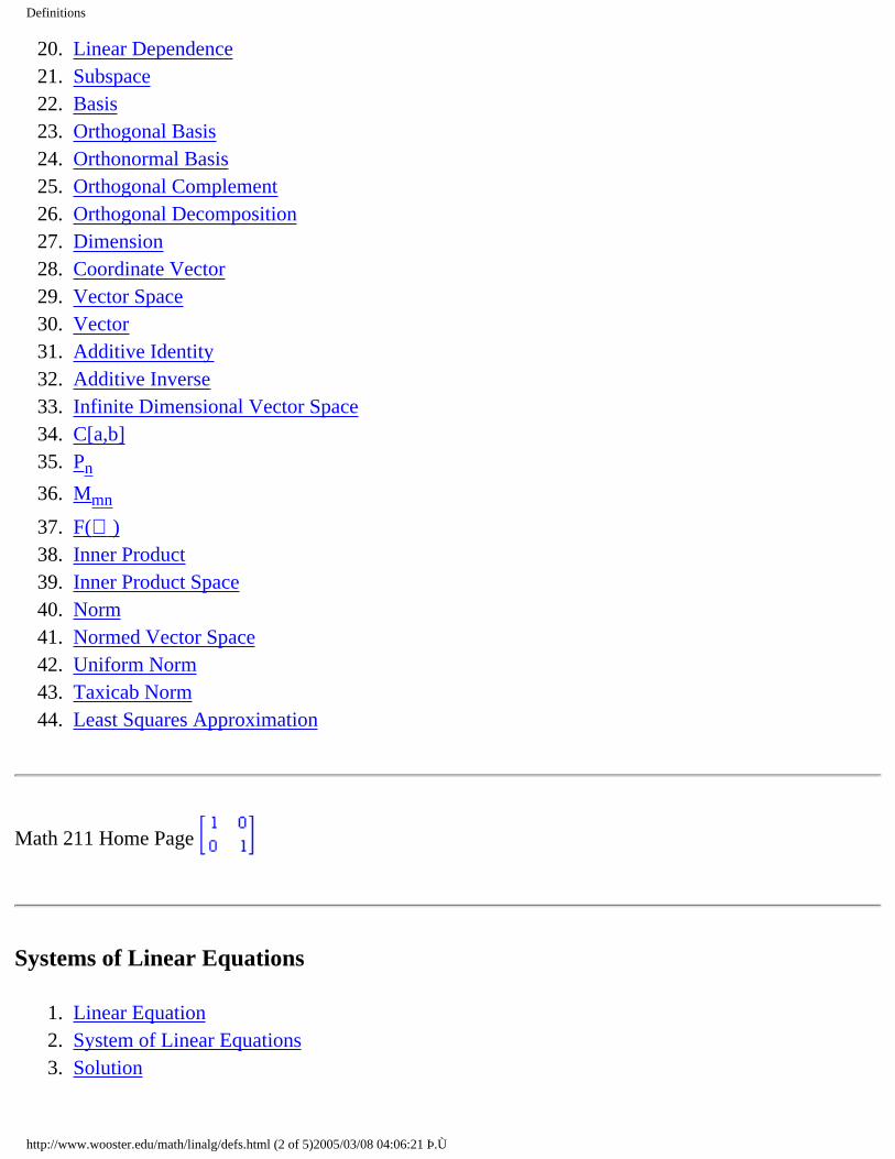
Linear Algebra and Applications Textbook
Welcome again. In order to enable prospective users to preview my text easily and conveniently, I'm putting a copy of it on the web for your perusal. The table of contents with links is at the bottom of this page. A few comments:
Why this text? I'm committed to a balanced blend of theory, application and computation. Mathematicians are beginning to see their discipline as more of an experimental science, with computer software as the "laboratory" for mathematical experimentation. I believe that the teaching of linear algebra should incorporate this new perspective. My own experience ranges from pure mathematician (my first research was in group and ring theory) to numerical analyst (my current speciality). I've seen linear algebra from many viewpoints and I think they all have something to offer. My computational experience makes me like the use of technology in the course -- a natural fit for linear algebra -- and computer exercises and group projects also fit very well into the context of linear algebra. My applied math background colors my choice and emphasis of applications and topics. At the same time, I have a traditionalist streak that expects a text to be rigorous, correct and complete. After all, linear algebra also serves as a bridge course between lower and higher level mathematics.
Many thanks to those who have helped me in this project. In particular, John Bakula for prodding me into moving this project into the final stages and pointed me in the direction of McGraw-Hill custom publishing. They are printing a nice soft copy text for a reasonable price to students -- about $26. Thanks also to my colleagues Jamie Radcliffe, Lynn Erbe, Brian Harbourne, Kristie Pfabe, Barton Willis and a number of others who have made many suggestions and corrections. Thanks to Jackie Kohles for her excellent work on solutions to the exercises.
http://www.math.unl.edu/~tshores/linalgtext.html (1 of 5)2005/03/08 04:09:38 Þ.Ù

Linear Algebra and Applications Textbook
About the process: I am writing the text in Latex. The pages you will see have been converted to gif files for universal viewing with most browsers. The downside of this conversion is that the pages appear at a fairly crude resolution. I hope that they are still readable to all. Hardcopy of the text is much prettier. Book form of the text can be purchased from McGraw-Hill Primus Custom Publishing. The ISBN for the text is 0072437693. An errata sheet for the text is provided below. In the near future, I will post a corrected version of the text on this website, though I don't know when or if there will be a published corrected version. If you have any suggestions or comments, drop me a line. I appreciate any feedback.
Applied Linear Algebra and Matrix Analysis
byThomas S. Shores
Copyright © November 2003 All Rights Reserved
Title Page Preface
Chapter 1. LINEAR SYSTEMS OF EQUATIONS
1. Some Examples
2. Notations and a Review of Numbers
3. Gaussian Elimination: Basic Ideas
4. Gaussian Elimination: General Procedure
5. *Computational Notes and Projects
Review Exercises
http://www.math.unl.edu/~tshores/linalgtext.html (2 of 5)2005/03/08 04:09:38 Þ.Ù

Linear Algebra and Applications Textbook
Chapter 2. MATRIX ALGEBRA
1. Matrix Addition and Scalar Multiplication
2. Matrix Multiplication
3. Applications of Matrix Arithmetic
4. Special Matrices and Transposes
5. Matrix Inverses
6. Basic Properties of Determinants
7. *Applications and Proofs for Determinants
8. *Tensor Products
9. *Computational Notes and Projects
Review Exercises
Chapter 3. VECTOR SPACES
1. Definitions and Basic Concepts
2. Subspaces
3. Linear Combinations
4. Subspaces Associated with Matrices and Operators
5. Bases and Dimension
6. Linear Systems Revisited
7. *Change of Basis and Linear Operators
8. *Computational Notes and Projects
http://www.math.unl.edu/~tshores/linalgtext.html (3 of 5)2005/03/08 04:09:38 Þ.Ù

Linear Algebra and Applications Textbook
Review Exercises
Chapter 4. GEOMETRICAL ASPECTS OF STANDARD SPACES
1. Standard Norm and Inner Product
2. Applications of Norm and Inner Product
3. Unitary and Orthogonal Matrices
4. *Computational Notes and Projects
5. Review Exercises
Chapter 5. THE EIGENVALUE PROBLEM
1. Definitions and Basic Properties
2. Similarity and Diagonalization
3. Applications to Discrete Dynamical Systems
4. Orthogonal Diagonalization
5. *Schur Form and Applications
6. *The Singular Value Decomposition
7. *Computational Notes and Projects
Review Exercises
Chapter 6. GEOMETRICAL ASPECTS OF ABSTRACT SPACES
1. Normed Linear Spaces
http://www.math.unl.edu/~tshores/linalgtext.html (4 of 5)2005/03/08 04:09:38 Þ.Ù

Linear Algebra and Applications Textbook
2. Inner Product Spaces
3. Gram-Schmidt Algorithm
4. Linear Systems Revisited
5. *Operator Norms
6. *Computational Notes and Projects
Review Exercises
Appendix A.
Table of Symbols
Solutions to Selected Exercises
Bibliography
Index
Errata Sheet for the third edition in pdf format
[ T O P ] [ H O M E ] [ S C H E D U L E ] [ T E A C H I N G ] R E S E A R C H ]
[ U N L ] [ A & S C O L L E G E ] [ M A T H / S T A T D E P T ]
http://www.math.unl.edu/~tshores/linalgtext.html (5 of 5)2005/03/08 04:09:38 Þ.Ù

ATLAST Project
Welcome to the ATLAST Project Forum
The Second Edition of the ATLAST book is now available.
The second edition of ATLAST Computer Exercises for Linear Algebra is now available. Instructors should contact their Prentice-Hall sales representatives to obtain copies and ordering information. The ATLAST book can be used in conjunction with any Linear Algebra textbook. The new edition contains more exercises and projects plus new and updated M-files.
Special Deal - The ATLAST book is being offered as a bundle with the Linear Algebra with Applications, 6th ed., by Steven J. Leon. The two book bundle is offered at the same price as the Leon textbook alone, so the ATLAST book is essentially free! The ISBN for the two book bundle is 0-13-104421-4.
Download the M-files for the second edition.
is a trademark for the MATLAB software distributed by the Mathworks of Natick, MA. The ATLAST M-files are add-on MATLAB programs. The M-files that accompany the second edition of the ATLAST book are fully compatible with version 6.5 of MATLAB. About a dozen new M-files were developed for the second edition. Click on the link below to download a zip file containing the complete collection of M-files for the second edition.
Download M-files for second edition.
http://www.umassd.edu/SpecialPrograms/Atlast/welcome.html (1 of 4)2005/03/08 04:10:12 Þ.Ù

ATLAST Project
About ATLAST
ATLAST is a National Science Foundation sponsored project to encourage and facilitate the use of software in teaching linear algebra. The project has received the support of two NSF DUE grants as part of their Undergraduate Faculty Enhancement program. The materials on this web page represent the opinions of its authors and not necessarily those of the NSF.
The ATLAST project conducted eighteen faculty workshops during the six summers from 1992 to 1997. The workshops were held at thirteen regional sites. A total of 425 faculty from a wide variety of colleges and universities participated in the workshops.
Workshop participants were trained in the use of the MATLAB software package and how to use software as part of classroom lectures. Participants worked in groups to design computer exercises and projects suitable for use in undergraduate linear algebra courses. These exercises were class tested during the school year following the workshop and then submitted for inclusion in a database. A comprehensive set of exercises from this database covering all aspects of the first course in linear algebra has been selected for a book ATLAST Computer Exercises for Linear Algebra. The editors of the book are Steven Leon, Eugene Herman, and Richard Faulkenberry. The later ATLAST workshops developed a series of lesson plans using software to enhance linear algebra classroom presentations. These lesson plans were adapted into the exercise/project format used in the ATLAST book and included in the second edition of the ATLAST book. The second edition of the ATLAST book is available from Prentice Hall.
The ATLAST Project is coordinated through the University of Massachusetts Dartmouth. The ATLAST Project Director is Steven Leon and the Assistant Director is Richard Faulkenberry. ATLAST Workshops have been presented by Jane Day, San Jose State University, Eugene Herman, Grinnell College, Dave Hill, Temple University, Kermit Sigmon, University of Florida, Lila Roberts, Georgia Southern University, and Steven Leon.
Software
● MATLAB
The software used for the ATLAST workshops has been MATLAB. The ATLAST organizers believe that MATLAB is the software of choice for teaching linear algebra. A student version of MATLAB is available from the MathWorks.
http://www.umassd.edu/SpecialPrograms/Atlast/welcome.html (2 of 4)2005/03/08 04:10:12 Þ.Ù

ATLAST Project
● Mathematica
Mathematica versions of most of the exercises and projects in the first edition of the ATLAST book are available. A collection of ATLAST Mathematica Notebooks has been developed by Richard Neidingerof Davidson College. The collection of notebooks can be downloaded from this link Mathematica Notebooks.
● Maple
We are looking for somebody to develop Maple versions of the of the exercises and projects in the second edition of the ATLAST book. If you are interested in doing this, please contact Steve Leon at the address given at the bottom of this Web page.
Lesson Plans
A selection of the ATLAST lesson are available for download.
ATLAST Lesson Plans
The Past and the Future . . .
● The History of the ATLAST project● List of the ATLAST contributors● Acknowledgements● Future Plans
If you have any questions, suggestions, or concerns about the ATLAST Project please contact:
Steven J. Leon ATLAST Project Director Department of Mathematics
University of Massachusetts Dartmouth North Dartmouth, MA 02747-2300
http://www.umassd.edu/SpecialPrograms/Atlast/welcome.html (3 of 4)2005/03/08 04:10:12 Þ.Ù

ATLAST Project
Telephone: (508) 999-8320 Fax: (508) 910-6917
Email: [email protected] or [email protected]
Originally created by (asb)
http://www.umassd.edu/SpecialPrograms/Atlast/welcome.html (4 of 4)2005/03/08 04:10:12 Þ.Ù

Linear Algebra Toolkit
© 2000−2002 P. Bogacki
Linear Algebra Toolkit - Main Page v. 1.23
This Linear Algebra Toolkit is comprised of the modules listed below. Each module is designed to help a linear algebra student learn and practice a basic linear algebra procedure, such as Gauss-Jordan reduction, calculating the determinant, or checking for linear independence.
Click here for additional information on the toolkit.
MODULES
Systems of linear equations and matrices
Row operation calculator Interactively perform a sequence of elementary row operations on the given m x n matrix A.
Transforming a matrix to row echelon form Find a matrix in row echelon form that is row equivalent to the given m x n matrix A.
Transforming a matrix to reduced row echelon form
Find the matrix in reduced row echelon form that is row equivalent to the given m x n matrix A.
Solving a linear system of equations Solve the given linear system of m equations in n unknowns.
Calculating the inverse using row operations Find (if possible) the inverse of the given n x n matrix A.
Determinants
Calculating the determinant using row operations
Calculate the determinant of the given n x n matrix A.
Vector spaces
Linear independence and dependenceGiven the set S = {v1, v2, ... , vn} of vectors in
the vector space V, determine whether S is linearly independent or linearly dependent.
http://www.math.odu.edu/~bogacki/cgi-bin/lat.cgi (1 of 3)2005/03/08 04:10:34 Þ.Ù

Linear Algebra Toolkit
Determining if the set spans the spaceGiven the set S = {v1, v2, ... , vn} of vectors in
the vector space V, determine whether S spans V.
Finding a basis of the space spanned by the setGiven the set S = {v1, v2, ... , vn} of vectors in
the vector space V, find a basis for span S.
Finding a basis of the null space of a matrixFind a basis of the null space of the given m x n matrix A. (Also discussed: rank and nullity of A.)
Linear transformations
Finding the kernel of the linear transformationFind the kernel of the linear transformation L: V→W. (Also discussed: nullity of L; is L one-to-one?)
Finding the range of the linear transformationFind the range of the linear transformation L: V→W. (Also discussed: rank of L; is L onto W?)
ADDITIONAL INFO
● The Linear Algebra Toolkit has been written entirely in PERL. Every effort has been made to make it compatible with a broad range of browsers, however, no guarantee can be made that every browser will properly handle this application.
● In order to bookmark the toolkit, first go to the cover page; all the other pages in this toolkit (including the one you are reading) are created dynamically.
● The toolkit represents all the data (such as matrix entries, vector components and polynomial coefficients) as rational numbers, where both the numerator and denominator are stored as integers. All operations on these rational numbers are performed exactly. Note that in the current version overflow errors are not trapped.
● Permission is hereby granted for any noncommercial use of this product by individuals, e.g. students, faculty, etc. Permission for the class use of this product in an academic environment is automatically granted, provided the instructor notifies the author. Any other use (including any commercial use) requires an explicit permission from the author.
http://www.math.odu.edu/~bogacki/cgi-bin/lat.cgi (2 of 3)2005/03/08 04:10:34 Þ.Ù

Linear Algebra Toolkit
● Comments should be forwarded to the author:
Przemyslaw Bogacki. Department of Mathematics and Statistics
Old Dominion University Norfolk, VA 23529
Phone: (757) 683-3262 E-mail: [email protected]
You can read testimonials from students and instructors who used the Toolkit.
● These pages should be considered work in progress. The interface and functionality will undergo changes as new versions are released. Here is a list of all released versions:
Version Date released Description
1.00 May 6, 2000 Row Operation Calculator
1.20 September 6, 2000ROC becomes Linear Algebra Toolkit 5 modules added
1.21 October 17, 2000 2 modules added
1.22 October 26, 2000 First official (non-beta) release
1.22a November 27, 2000 Bug fixes
1.23 October 25, 2002 2 modules added
http://www.math.odu.edu/~bogacki/cgi-bin/lat.cgi (3 of 3)2005/03/08 04:10:34 Þ.Ù
Elements of Abstract and Linear Algebra by Edwin H. Connell
Elements of Abstract and Linear Algebra Edwin H. Connell
This is a foundational textbook on abstract algebra with emphasis on linear algebra. You may download parts of the book or the entire textbook. It is
provided free online in PDF, DVI, postscript, and gzipped postscript.
Please read some words from the author first.
Join the revolution in education! Write a supplement to this book and put it online.
Participate in and contribute to a forum on abstract and linear algebra. Ask questions, give answers, and make comments in a worldwide classroom with the internet as blackboard.
[March 20, 2004]
The entire book
Title page and copyright
Introduction
Outline
Chapter 1: Background and Fundamentals of Mathematics
Chapter 2: Groups
Chapter 3: Rings
Chapter 4: Matrices and Matrix Rings
Chapter 5: Linear Algebra
Chapter 6: Appendix
http://www.math.miami.edu/~ec/book/ (1 of 2)2005/03/08 04:11:04 Þ.Ù

Elements of Abstract and Linear Algebra by Edwin H. Connell
Index
Please send comments to Edwin H. Connell Web page created by Dmitry Gokhman
http://www.math.miami.edu/~ec/book/ (2 of 2)2005/03/08 04:11:04 Þ.Ù

Linear Algebra textbook home page
Linear Algebra
by Jim Hefferon Mathematics Saint Michael's College Colchester, Vermont USA 05439
My text Linear Algebra is free for downloading, It covers the material of an undergraduate first linear algebra course. You can use it either as a main text, or as a supplement to another text, or for independent study.
What's Linear Algebra About?
When I started teaching linear algebra I found three kinds of texts. There were applied mathematics books that avoid proofs and cover the linear algebra only as needed for their applications. There were advanced books that assume that students can understand their elegant proofs and understand how to answer the homework questions having seen only one or two examples. And there were books that spend a good part of the semester doing elementary things such as multiplying matrices and computing determinants and then suddenly change level to working with definitions and proofs.
Each of these three types was a problem in my classroom. The applications were interesting, but I wanted to focus on the linear algebra. The advanced books were beautiful, but my students were not ready for them. And the level-switching books resulted in a lot of grief. My students immediately thought that these were like the calculus books that they had seen before, where there is material labelled `proof' that they have successfully skipped in favor of the computations. Then, by the time that the level switched, no amount of prompting on my part could convince them otherwise and the semesters ended unhappily.
That is, while I wish I could say that my students now perform at the level of the advanced books, I cannot. However, we can instead work steadily to bring them up to it, over the course of our program. This means stepping back from rote computations of the application books in favor of an understanding of the mathematics. It means proving things and having them understand, e.g., that matrix multiplication is the application of a linear function. But it means also avoiding an approach that is too advanced for the students; the presentation must emphasize motivation, must have many exercises, and must include problem sets with many of the medium-difficult questions that are a challenge to a learner without being overwhelming. And, it means communicating to our students that this is what we are doing, right from
http://joshua.smcvt.edu/linearalgebra/ (1 of 4)2005/03/08 04:11:18 Þ.Ù

Linear Algebra textbook home page
the start.
Summary Points
● The coverage is standard: linear systems and Gauss' method, vector spaces, linear maps and matrices, determinants, and eigenvectors and eigenvalues. The Table of Contents gives you a quick overview.
● Prerequisites A semester of calculus. Students with three semesters of calculus can skip a few sections.
● Applications Each chapter has three or four discussions of additional topics and applications. These are suitable for independent study or for small group work.
● What makes this book different? Its approach is developmental. Although the presentation is focused on proving things and covering linear algebra, it does not start with an assumption that students are already able at abstract work. Instead, it proceeds with a great deal of motivation, and many examples and exercises that range from routine verifications to (a few) challenges. The goal is, in the context of developing the usual material of an undergraduate linear algebra course, to help raise the level of mathematical maturity of the class.
There is only one review that I know of.
Here Is Linear Algebra
The files are current as of 2003-May-05. To have a look at the PDF files you need Adobe Acrobat. (Note for those with limited Internet access: this material is available as part of the eGranary Project; perhaps that will help you)
● The whole book Linear Algebra along with the answers to all exercises or just the answers to checked exercises. If you save the two files in the same directory then clicking on an exercise will send you to its answer and clicking on an answer will send you to its exercise. (You will need to rename the file "jhanswer.pdf" to use the hyperlink feature. Note Natalie Kehr has sent me a suggestion for people wanting to access the answers in this way. "In Acrobat reader go to Edit | Preferences | General and uncheck the box for Open cross-document links in same window. Also, a possible reasonable way of working is to click on the hyperlink to get from the question to the answer, but to return by closing the answer window. By using hyperlinks both ways, without realizing it I eventually landed up with dozens of open windows. Another good technique is to use a single hyperlink and then use Alt W 1 and Alt W 2 to toggle between the two windows.")
● The first chapter, on linear elimination. ● The second chapter, on vector spaces.
http://joshua.smcvt.edu/linearalgebra/ (2 of 4)2005/03/08 04:11:18 Þ.Ù

Linear Algebra textbook home page
● The third chapter, on linear maps and matrix operations. ● The fourth chapter on determinants. ● The fifth chapter, on matrix similarity and Jordan form. ● The source. You need to know LaTeX and MetaPost to work with it, although there is a readme
file to get you going. Also there is a bit of optional material, and a version of the book and answers in PostScript that has been zipped.
If you just want a quick look, try the second chapter. The first chapter may be misleading because it is necessarily computational but the second chapter shows clearly what the book works on: bridging between high school mathematics with its reliance on explicitly-given algorithms and upper division college mathematics with its emphasis on concepts and proof.
Naturally, I'd be glad for any comments or interest in trying it out. It's been class-tested here and elsewhere, and I'm delighted to have it on student's desks, doing what it is for. Around here, running off double-sided copies and comb-binding them costs students $20.00 (we include the Preface, Table of Contents, Appendix, and Index to make 449 pages. With the Answers to Exercises at 213 pages the total is $25.00).
Can You Help With Linear Algebra?
In addition to the book, the answers to the exercises, and the source, you can get some materials that were contributed by others. If you in turn have something that you are able to share please write me. Anything is welcome, from a suggestion about a better way to prove a result or make an example, to an entire Topic or subsection. In particular, your used exams or problem sets would be very welcome, especially if you can contribute the TeX or LaTeX source, so that a user could cut or paste. Several people have asked me about a Topic on eigenvectors and eigenvalues in Quantum Mechanics. Sadly, I don't know any QM. Can you help?
One point about contacting me with typo and bug reports: I receive such reports from many people and they are a big help. I save them and once in a while do a batch of updates, so if you made a report and it hasn't gotten addressed yet, please be patient. Conversely, for those people who have gotten these materials on a disk, please be aware that there is probably a more recent version on-line and you can check there for updates, if possible.
Naturally, all contributions will be gratefully acknowledged (or anonymous, if you like).
Has Linear Algebra Helped You?
http://joshua.smcvt.edu/linearalgebra/ (3 of 4)2005/03/08 04:11:18 Þ.Ù

Linear Algebra textbook home page
If you find the book useful, drop me a note in the mail. In particular, if you use it in a class, a letter on letterhead to the address below would be great.
Jim Hefferon Mathematics, Saint Michael's College Winooski Park Colchester, VT USA, 05439
Some people don't believe me when I tell them that I'm working in here.
Page Information
The page above. The page maintainer is Jim Hefferon.
This site Joshua is located in the Mathematics Department of Saint Michael's College in Colchester, Vermont USA. Joshua runs under Linux. Open Source software is a great idea. This project would not
have gotten done without it.
(Credit for the logo to Matt Ericson.)
http://joshua.smcvt.edu/linearalgebra/ (4 of 4)2005/03/08 04:11:18 Þ.Ù

ELEMENTARY LINEAR ALGEBRA
Elementary Linear Algebra
(Lecture Notes by Keith Matthews, 1991)
CMAT: An exact arithmetic matrix calculator program
● Preface ● Title Page/Contents (pages 0, i-iv)
❍ pdf version of book (731K) ● Chapter 1: Linear Equations (pages 1-21) ● Chapter 2: Matrices (pages 23-54) ● Chapter 3: Subspaces (pages 55-70) ● Chapter 4: Determinants (pages 71-88) ● Chapter 5: Complex Numbers (pages 89-114) ● Chapter 6: Eigenvalues and Eigenvectors (pages 115-128) ● Chapter 7: Identifying Second Degree Equations (pages 129-148) ● Chapter 8: Three-dimensional Geometry (pages 149-187) ● Further Reading/Bibliography (pages 189,191-193) ● Index (pages 194-196)
● Corrections
Solutions to Elementary Linear Algebra
(Prepared by Keith Matthews, 1991)
● Title Page/Contents (pages 0/i) ❍ pdf version of the solutions (437K - best read with zoom in)
● Problems 1.6: Linear Equations (pages 1-11) ● Problems 2.4: Matrices (pages 12-17) ● Problems 2.7: Matrices (pages 18-31) ● Problems 3.6: Subspaces (pages 32-44) ● Problems 4.1: Determinants (pages 45-57) ● Problems 5.8: Complex Numbers (pages 58-68) ● Problems 6.3: Eigenvalues and Eigenvectors (pages 69-82) ● Problems 7.3: Identifying Second Degree Equations (pages 83-90)
http://www.numbertheory.org/book/ (1 of 2)2005/03/08 04:11:22 Þ.Ù

ELEMENTARY LINEAR ALGEBRA
● Problems 8.8: Three-dimensional Geometry (pages 91-103)
Last modified 10th December 2004
http://www.numbertheory.org/book/ (2 of 2)2005/03/08 04:11:22 Þ.Ù

Lee Lady: Notes on Linear Algebra
Notes on Linear Algebra
Professor Lee Lady
University of Hawaii
Mostly there are two themes in this collection of short hand-outs. First, that rather than think of an m by n matrix as a doubly-indexed array, it is often more enlightening to think of it as a n-tuple of columns (which are, of course, m-vectors) or an m-tuple of rows. And secondly, that once one understands the method of solving systems of equations by elimination, essentially one knows the whole of the linear algebra covered in this (very stripped-down) course. Everything else, except for eigenvectors and eigenvalues, is just a matter of constantly restating the same facts in different language.
A lot of the files listed below are in PDF (Adobe Acrobat) format. Alternate versions are in DVI format (produced by TeX; see see here for a DVI viewer provided by John P. Costella) and postscript format (viewable with ghostscript.) Some systems may have some problem with certain of the documents in dvi format, because they use a few German letters from a font that may not be available on some systems. (Three alternate sites for DVI viewers, via FTP, are CTAN, Duke, and Dante, in Germany.)
Systems of Linear Equations in a Nutshell
(Click here for dvi format.)(Click here for Postscript format.)
Instead of thinking of a systems of equations as constituting m equations in n unknowns, where all the coefficients are scalars, it can be more enlightening to think of it as a single equation in n unknowns where the coefficients (and constant term) are m-dimensional vectors.
http://www.math.hawaii.edu/%7Elee/linear/ (1 of 4)2005/03/08 04:11:39 Þ.Ù

Lee Lady: Notes on Linear Algebra
How to Find the Inverse of a Matrix
(Click here for dvi format.)(Click here for Postscript format format.)
Doing an elementary row operation on the left-hand factor A of a matrix product AB gives the same result as doing the same operation on the product matrix. Using this observation, it is easy to explain why the usual process for inverting a matrix works, and why the left inverse and the right inverse are identical. This approach enables one to omit the topic of elementary matrices from the course.
Some Equivalent Statements
(Click here for dvi format.)(Click here for Postscript format.)
Some Equivalent Characterizations of Basic Concepts
(Click here for dvi format.)(Click here for Postscript format.)
A ``Grammar Lesson'' in Linear Algebra
(Click here for dvi format.)(Click here for Postscript format.)
Some incorrect statements frequently found in student proofs.
The Pivotal Role of Zero in Linear Algebra
http://www.math.hawaii.edu/%7Elee/linear/ (2 of 4)2005/03/08 04:11:39 Þ.Ù

Lee Lady: Notes on Linear Algebra
(Click here for dvi format.)(Click here for Postscript format.)
The Logical Structure of Proving Linear Independence
(Click here for dvi format.)(Click here for Postscript format.)
Students seem to have enormous difficulty in learning the pattern for proving any statement that essentially reduces to an implication, such as proving that vectors are linearly independent or that a function is one-to-one. (This may also be a main source of the difficulty students have with proofs by induction.) When asked to prove "If P, then Q," students will almost invariably begin by saying, "Suppose Q." The logical analysis here was one of my attempts to clarify this type of proof for students. I don't know whether it actually helps or not.
The Column Space of a Matrix
(Click here for dvi format.)(Click here for Postscript format.)
By definition, the column space of an m by n matrix A with entries in a field F is the subspace of Fm spanned by the columns of A. A close examination of the method of elimination shows that a basis for this space can be obtained by choosing those columns of A which will contain the leading entries of rows after A is reduced to row-echelon form. (The row echelon form of A shows which columns to choose, but the basis columns themselves must come from the original matrix A.)
Eigenvalues
(Click here for dvi format.)
http://www.math.hawaii.edu/%7Elee/linear/ (3 of 4)2005/03/08 04:11:39 Þ.Ù

Lee Lady: Notes on Linear Algebra
(Click here for Postscript format.)
Suppose than an n by n matrix A has n linearly independent eigenvectors and let P be the matrix whose columns are these eigenvectors. Then the jth column of the product AP is readily seen to be equal to the jth column of P multiplied by the jth eigenvalue. If now we write Q for the inverse of P, it follows easily that QAP is a diagonal matrix with the eigenvalues on the diagonal. This approach is not dependent on change-of-basis formulas.
Syllabus for Spring, 1996
[ Top of Page | Calculus | HOME ]
This page has been accessed times
http://www.math.hawaii.edu/%7Elee/linear/ (4 of 4)2005/03/08 04:11:39 Þ.Ù

Electronic Journal of Linear Algebra
ELECTRONIC Journal of LINEAR ALGEBRA
Published by ILAS - The International Linear Algebra Society
ISSN 1081-3810
Primary Site: Israel
Mirror Sites: USA Germany Portugal EMIS Other EMIS sites
Editors in Chief:
Ludwig Elsner
Daniel Hershkowitz
Advisory Editors:
Ravindra B. Bapat
Richard A. Brualdi
Miroslav Fiedler
Shmuel Friedland
Stephen J. Kirkland
Peter Lancaster
Hans Schneider
Bryan L. Shader
Daniel B. Szyld
Associate Editors:
Harm Bart Robert Guralnick Michael Neumann Bit-Shun Tam
Managing Editor:
http://hermite.cii.fc.ul.pt/iic/ela/ (1 of 4)2005/03/08 04:12:13 Þ.Ù

Electronic Journal of Linear Algebra
Daniel Hershkowitz
Associate Managing Editor:
Michael J. Tsatsomeros
Assistant Managing Editor:
Shaun Fallat
Editors' e-mail addresses Editors' Postal addresses Former editors
Volume 14 (2005) Table of Contents Articles Author Index
Volume 13 (2005) Table of Contents Articles Author Index
Volume 12 (2004/2005) Table of Contents Articles Author Index
Volume 11 (2004) Table of Contents Articles Author Index
Volume 10 (2003) Table of Contents Articles Author Index
Volume 9 (2002) Table of Contents Articles Author Index
Volume 8 (2001) Table of Contents Articles Author Index
Volume 7 (2000) Table of Contents Articles Author Index
Volume 6 (1999/2000) Table of Contents Articles Author Index
Volume 5 (1999) Table of Contents Articles Author Index
Volume 4 (1998) Table of Contents Articles Author Index
Volume 3 (1998) Table of Contents Articles Author Index
Volume 2 (1997) Table of Contents Articles Author Index
Volume 1 (1996) Table of Contents Articles Author Index
http://hermite.cii.fc.ul.pt/iic/ela/ (2 of 4)2005/03/08 04:12:13 Þ.Ù

Electronic Journal of Linear Algebra
Multi-year Author Index:
A B C D E F G H I J K L M N O P Q R S T U V W X Y Z
ELA guide:
preparing an article submitting an article reading and downloading
ELA Information about:
the Electronic Journal Copyrights Transfer Agreement
PRINT VERSION OF ELA
ELA-LIST
IIC - ILAS Information Center
Click to send your comments to ELA
Your visit here is number
Since March 1, 1999 Links2Go
Mathematical Journals
http://hermite.cii.fc.ul.pt/iic/ela/ (3 of 4)2005/03/08 04:12:13 Þ.Ù

Electronic Journal of Linear Algebra
http://hermite.cii.fc.ul.pt/iic/ela/ (4 of 4)2005/03/08 04:12:13 Þ.Ù

Down with Determinants!
Down with Determinants!
Sheldon Axler
This paper was published in the American Mathematical Monthly 102 (1995), 139-154.
In 1996 this paper received the Lester R. Ford Award for expository writing from the Mathematical Association of America.
Abstract: This paper shows how linear algebra can be done better without determinants. The standard proof that a square matrix of complex numbers has an eigenvalue uses determinants. The simpler and clearer proof presented here provides more insight and avoids determinants. Without using determinants, this allows us to define the multiplicity of an eigenvalue and to prove that the number of eigenvalues, counting multiplicities, equals the dimension of the underlying space. Without using determinants, we can define the characteristic and minimal polynomials and then prove that they behave as expected. This leads to an easy proof that every matrix is similar to a nice upper-triangular one. Turning to inner product spaces, and still without mentioning determinants, this paper gives a simple proof of the finite-dimensional spectral theorem.
To obtain the entire paper, select your choice below:
● pdf version ● dvi version ● PostScript version
My book Linear Algebra Done Right is partly based on ideas from this paper. The book is intended to be a text for a second course in linear algebra.
http://www.axler.net/DwD.html (1 of 2)2005/03/08 04:12:34 Þ.Ù

Down with Determinants!
● Sheldon Axler's publications
● Sheldon Axler's home page
http://www.axler.net/DwD.html (2 of 2)2005/03/08 04:12:34 Þ.Ù

Linear Algebra Glossary
Linear Algebra Glossary
This file defines common terms from linear algebra.
TABLE OF CONTENTS
● A-Orthogonal Vectors ● Adjacency Matrix ● Adjoint Matrix ● Alternating Sign Matrix ● Anticirculant Matrix ● Antisymmetric Matrix ● Band Matrix ● Band Matrix Storage ● Bandwidth ● Basis ● Bidiagonal Matrix ● Basic Linear Algebra Subprograms (BLAS) ● Block Matrix ● Border Banded Matrix ● Cartesian_Basis_Vectors ● The Cauchy-Schwarz Inequality ● The Cayley-Hamilton Theorem ● CentroSymmetric Matrix ● Characteristic Equation ● Cholesky Factorization ● Circulant Matrix ● Cofactor Matrix ● Column Echelon Form ● Commuting Matrices ● Companion Matrix ● Compatible Norms ● Complex Number Representation ● Condition Number ● Congruent Matrix ● Conjugate Gradient Method
http://www.psc.edu/%7Eburkardt/papers/linear_glossary.html (1 of 151)2005/03/08 04:13:36 Þ.Ù

Linear Algebra Glossary
● Conjugate Matrix ● Conjugate of a Complex Number ● Conjunctive Matrix ● Convergent Matrix ● Cross Product ● Cyclic Reduction ● Cyclic Tridiagonal Matrix ● Defective Matrix ● Deflation ● Derogatory Matrix ● Determinant of a Matrix ● Diagonal Dominance ● Diagonal Matrix ● Diagonalizable Matrix ● Downshift Matrix ● Eigenvalues ● Eigenvectors ● EISPACK ● EISPACK Matrix Norm ● Elementary Column Operations ● Elementary Matrix ● Elementary Row Operations ● Ellipsoids ● Equilibration ● Equivalent Matrix ● Exchange Matrix ● External Storage Algorithms ● Fourier Matrix ● Frobenius Matrix Norm ● Gauss Elimination ● Gauss Jordan Elimination ● Gauss Seidel Iteration For Linear Equations ● General Matrix Storage ● Generalized Permutation Matrix ● Gershgorin Disks ● Givens Rotation Matrix ● Gram Schmidt Orthogonalization ● Hadamard's Inequality
http://www.psc.edu/%7Eburkardt/papers/linear_glossary.html (2 of 151)2005/03/08 04:13:36 Þ.Ù

Linear Algebra Glossary
● Hadamard Product ● Hankel Matrix ● Harwell Boeing Sparse Matrix Collection (HBSMC) ● HBSMC Sparse Matrix Storage ● HBSMC Finite Element Matrix Storage ● Hermite Normal Form ● Hermitian Matrix ● Hessenberg Matrix ● Householder Matrix ● Idempotent Matrix ● The Identity Matrix ● Ill Conditioned Linear System ● The Incomplete LU Factorization ● Inertia ● Inner Product ● Inverse Matrix ● Inverse Power Method ● Invertible Matrix ● Involutory Matrix ● Irreducible Matrix ● Iterative Methods for Eigenvalues ● Iterative Methods for Linear Equations ● Iterative Refinement ● The Jacobi Algorithm for Eigenvalues ● The Jacobi Algorithm for Linear Equations ● The Jacobi Preconditioner ● Jordan Canonical Form ● L1 Matrix Norm ● L1 Vector Norm ● L2 Matrix Norm ● L2 Vector Norm ● L Infinity Matrix Norm ● L Infinity Vector Norm ● LAPACK ● LDL Factorization ● Linear Dependence ● Linear Least Squares Problems ● Linear Space
http://www.psc.edu/%7Eburkardt/papers/linear_glossary.html (3 of 151)2005/03/08 04:13:36 Þ.Ù

Linear Algebra Glossary
● Linear Transformation ● LINPACK ● LU Factorization ● M Matrix ● Magic Square ● Matrix Exponential ● Matrix Factorization ● Matrix Multiplication ● Matrix Norm ● Matrix_Order ● Matrix Properties ● Matrix Rank ● Matrix Splitting ● Matrix Square Root ● Matrix Storage ● Matrix Structure ● Matrix Symmetry ● Minimal Polynomial ● Minor Matrix ● Monic Polynomial ● Multiplicity ● Nilpotent Matrix ● Nonnegative Matrix ● Normal Equations ● Normal Matrix ● Null Space ● Null Vector ● Orthogonal Matrix ● Orthogonal Similarity Transformation ● Orthonormal Vectors ● Outer Product ● Orthogonal Projector Matrix ● Overdetermined System ● Permanent of a Matrix ● Permutation Matrix ● Perron-Frobenius Theorem ● Persymmetric Matrix ● Pivoting
http://www.psc.edu/%7Eburkardt/papers/linear_glossary.html (4 of 151)2005/03/08 04:13:36 Þ.Ù

Linear Algebra Glossary
● Polar Decomposition ● Positive definite matrix ● Positive Matrix ● The Power Method ● Preconditioner ● Property A ● The Pseudoinverse ● QR Factorization ● QR Method for Eigenvalues ● Quaternion Representation ● Rayleigh Quotient ● Rectangular Matrix ● Reflection Matrix ● Residual Error ● Root of Unity ● Rotation ● Row Echelon Form ● Row Rank ● Row Space ● The Schur Decomposition ● Sherman Morrison Formula ● Sign Symmetric Matrix ● Similar Matrix ● Singular Matrix ● Singular Value Decomposition ● Skew CentroSymmetric Matrix ● Skew Hermitian Matrix ● Skyline Matrix Storage ● Span of a Set of Vectors ● The Sparse BLAS ● Sparse Matrix ● Sparse Matrix Storage ● SPARSKIT ● Spectral Radius ● Spectrum ● Square Matrix ● Stochastic Matrix ● Strassen's Algorithm
http://www.psc.edu/%7Eburkardt/papers/linear_glossary.html (5 of 151)2005/03/08 04:13:36 Þ.Ù

Linear Algebra Glossary
● Submatrix ● Successive Overrelaxation Method (SOR) ● Symmetric Matrix ● Symmetric Matrix Storage ● TESTMATRIX ● Toeplitz Matrix ● Trace of a Matrix ● Transpose ● Trapezoidal Matrix ● Triangular Matrix ● Tridiagonal Matrix ● Unimodular Matrix ● Unitary Matrix ● Unitary Similarity Transformation ● Upshift Matrix ● Vector-Bound Matrix Norm ● Vector Norm ● Zero Matrix ● Zero One Matrix
A-Orthogonal Vectors
Two vectors u and v are said to be A-orthogonal if
( u, A * v ) = 0.
Here A should be a positive definite symmetric matrix, which in turn guarantees that the expression ( u, A * v ) may be regarded as an inner product of the vectors u and v, with the usual properties.
This concept is useful in the analysis of the conjugate gradient method.
Back to TABLE OF CONTENTS.
Adjacency Matrix
An adjacency matrix of an (undirected) graph is a matrix whose order is the number of nodes, and whose entries record which nodes are connected to each other by a link or edge of the graph.
http://www.psc.edu/%7Eburkardt/papers/linear_glossary.html (6 of 151)2005/03/08 04:13:36 Þ.Ù

Linear Algebra Glossary
If two nodes I and J are connected by an edge, then Ai,j=1. All other entries of the matrix are 0. Thus, an
adjacency matrix is a zero-one matrix. The usual convention is that a node is not connected to itself, and hence the diagonal of the matrix is zero.
The product A2=A*A is a matrix which records the number of paths between nodes I and J. If it is possible to reach one node from another, it must be possible in a path of no more than n-1 links. Hence, the reachability matrix, which records whether it is possible to get from node I to node J in one or more steps, can be determined by taking the logical sum of the matrices I, A, A2, ..., An-1.
Back to TABLE OF CONTENTS.
Adjoint Matrix
The adjoint matrix of a square matrix A has the property that:
A * adjoint ( A ) = adjoint ( A ) * A = det(A) * I.
Thus, the adjoint of A is "almost" the inverse. If A is invertible, then the inverse of A, denoted inverse ( A ) can be written explicitly as:
A-1 = ( 1 / det(A) ) * adjoint ( A ).
The adjoint matrix, in turn, is defined in terms of the cofactor matrix of A:
adjoint ( A ) = ( cofactor ( A ) )T.
Back to TABLE OF CONTENTS.
Alternating Sign Matrix
An alternating sign matrix is an integer matrix with the properties that
● the entries are only 0, +1, or -1; ● the sum of the entries in each row and column is 1; ● the first (and last) nonzero entry in each row and column is 1; ● the nonzero entries in any row or column alternate in sign.
Example:
http://www.psc.edu/%7Eburkardt/papers/linear_glossary.html (7 of 151)2005/03/08 04:13:36 Þ.Ù
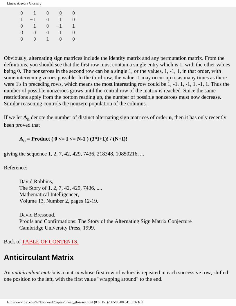
Linear Algebra Glossary
0 1 0 0 0 1 -1 0 1 0 0 1 0 -1 1 0 0 0 1 0 0 0 1 0 0
Obviously, alternating sign matrices include the identity matrix and any permutation matrix. From the definitions, you should see that the first row must contain a single entry which is 1, with the other values being 0. The nonzeroes in the second row can be a single 1, or the values, 1, -1, 1, in that order, with some intervening zeroes possible. In the third row, the value -1 may occur up to as many times as there were 1's in preceding rows, which means the most interesting row could be 1, -1, 1, -1, 1, -1, 1. Thus the number of possible nonzeroes grows until the central row of the matrix is reached. Since the same restrictions apply from the bottom reading up, the number of possible nonzeroes must now decrease. Similar reasoning controls the nonzero population of the columns.
If we let An denote the number of distinct alternating sign matrices of order n, then it has only recently
been proved that
An = Product ( 0 <= I <= N-1 ) (3*I+1)! / (N+I)!
giving the sequence 1, 2, 7, 42, 429, 7436, 218348, 10850216, ...
Reference:
David Robbins,The Story of 1, 2, 7, 42, 429, 7436, ...,Mathematical Intelligencer,Volume 13, Number 2, pages 12-19.
David Bressoud,Proofs and Confirmations: The Story of the Alternating Sign Matrix ConjectureCambridge University Press, 1999.
Back to TABLE OF CONTENTS.
Anticirculant Matrix
An anticirculant matrix is a matrix whose first row of values is repeated in each successive row, shifted one position to the left, with the first value "wrapping around" to the end.
http://www.psc.edu/%7Eburkardt/papers/linear_glossary.html (8 of 151)2005/03/08 04:13:36 Þ.Ù

Linear Algebra Glossary
Here is an example of an anticirculant matrix:
1 2 3 4 2 3 4 1 3 4 1 2 4 1 2 3
and here is an example of a rectangular anticirculant matrix:
1 2 3 4 5 2 3 4 5 1 3 4 5 1 2
Simple facts about a anticirculant matrix A:
● A is constant along any antidiagonal; ● A is a special kind of Hankel matrix; ● If A is square, then A is normal, hence unitarily diagonalizable. ● If A is square, then the vector (1,1,...,1) is an eigenvector of the matrix, with eigenvalue equal to
the sum of the entries of a row.
Back to TABLE OF CONTENTS.
Antisymmetric Matrix
A square matrix A is antisymmetric if it is equal to the negative of its transpose:
A = - AT.
Every matrix A can be decomposed into the sum of an antisymmetric and a symmetric matrix:
A = B + C = (1/2) * ( ( A - AT ) + ( A + AT ) )
Simple facts about an antisymmetric matrix A:
● A has a zero diagonal; ● A has pure imaginary eigenvalues; ● A is normal, hence unitarily diagonalizable. ● I - A is not singular;
http://www.psc.edu/%7Eburkardt/papers/linear_glossary.html (9 of 151)2005/03/08 04:13:36 Þ.Ù

Linear Algebra Glossary
● The matrix ( I + A ) * Inverse ( I - A ) is orthogonal;
An antisymmetric matrix is also called skew symmetric.
In complex arithmetic, the corresponding object is a skew Hermitian matrix.
Back to TABLE OF CONTENTS.
Band Matrix
A band matrix is a matrix whose entries are all zero except for the diagonal and a few of the immediately adjacent diagonals.
If the band matrix is large enough, then many significant efficiencies can be achieved in storage and matrix operations. Because so many elements are zero, the band matrix can be stored more compactly using band matrix storage. And because so many elements are zero, many algorithms can be speeded up to execute more quickly, including matrix multiplication and Gauss elimination.
Special cases include band matrices which are symmetric, positive definite, or tridiagonal.
Here is an example of a band matrix:
11 12 0 0 0 0 21 22 23 0 0 0 31 32 33 34 0 0 0 42 43 44 45 0 0 0 53 54 55 56 0 0 0 64 65 66
This matrix has an upper bandwidth of 1, and lower bandwidth of 2, and an overall bandwidth of 4.
LAPACK and LINPACK include special routines for a variety of band matrices. These routines can compute the LU factorization, determinant, inverse, or solution of a linear system.
LAPACK and EISPACK have routines for computing the eigenvalues of a symmetric banded matrix.
Back to TABLE OF CONTENTS.
Band Matrix Storage
http://www.psc.edu/%7Eburkardt/papers/linear_glossary.html (10 of 151)2005/03/08 04:13:36 Þ.Ù

Linear Algebra Glossary
Band matrix storage is a matrix storage format suitable for efficiently storing the nonzero entries of a band matrix.
Most band storage schemes are column oriented. The nonzero entries of the matrix "slide" downwards, while remaining in their original column. If the original matrix looked like this:
11 12 0 0 0 0 21 22 23 0 0 0 31 32 33 34 0 0 0 42 43 44 45 0 0 0 53 54 55 56 0 0 0 64 65 66
the matrix would be saved in column band matrix storage as:
0 12 23 34 0 0 11 22 33 44 45 0 21 32 43 54 55 56 31 42 53 64 65 66
Note that the zeroes in the above array are there just as padding. They don't correspond to any entries of the original array, and are simply necessary to make the array rectangular.
If the matrix is to be handled by a Gauss elimination routine that uses pivoting, then there is a possibility of fill in; that is, nonzero entries may need to be stored in places where zeroes had been. Band matrix storage can still be used, but we need to include in the compressed matrix some extra entries representing the diagonals along which the fill in entries may occur. It turns out that the number of extra diagonals required is simply the number of nonzero subdiagonals in the original matrix. For our example, this would mean the matrix would be stored as:
0 0 0 0 0 0 0 0 0 0 0 0 0 12 23 34 0 0 11 22 33 44 45 0 21 32 43 54 55 56 31 42 53 64 65 66
http://www.psc.edu/%7Eburkardt/papers/linear_glossary.html (11 of 151)2005/03/08 04:13:36 Þ.Ù

Linear Algebra Glossary
Back to TABLE OF CONTENTS.
Bandwidth
The bandwidth of a band matrix is, roughly speaking, the number of diagonals that contain nonzero entries.
More precisely, define ML, the lower bandwidth of a matrix A to be the maximum value of ( I - J ), and MU to be the maximum value of ( I - J ), for all nonzero matrix entries A(I,J). Then the bandwidth M is defined by:
M = ML + 1 + MU.
This definition always treats the (main) diagonal as nonzero, and is not misled by a matrix which has only two nonzero diagonals, which are actually widely separated. All the territory between the diagonals must be included when measuring bandwidth.
Back to TABLE OF CONTENTS.
Basis
A basis for a linear space X of dimension N is a set of N vectors, {v(i) | 1 <= i <= N } from which all the elements of X can be constructed by linear combinations.
Naturally, we require that each of the vectors v(i) be an element of the space X. Moreover, it is not enough that these vectors span the space; we also require that they be linearly independent, that is, there should be no redundant vectors in the set.
The columns of the identity matrix form a basis for the linear space of vectors of dimension N. A square matrix of order N is not defective exactly when its eigenvectors form a basis for the linear space of vectors of dimension N.
Given a particular basis, the representation of a vector x is the unique set of coefficients c(i) so that
x = Sum ( 1 <= I <= N ) c(i) * v(i)
The coefficients must be unique, otherwise you can prove that the basis is not linearly independent!
If the basis vectors are pairwise orthogonal, then the basis is called an orthogonal basis. If the basis
http://www.psc.edu/%7Eburkardt/papers/linear_glossary.html (12 of 151)2005/03/08 04:13:36 Þ.Ù

Linear Algebra Glossary
vectors have unit length in the Euclidean norm, the basis is a normal basis. If both properties apply, it is an orthonormal basis. The columns of an orthogonal matrix are an orthonormal basis for the linear space of vectors of dimension N.
Back to TABLE OF CONTENTS.
Bidiagonal Matrix
A bidiagonal matrix has only two nonzero diagonals. The matrix is called upper bidiagonal if these are the main diagonal and the immediate upper diagonal. The matrix is called lower bidiagonal if these are the main diagonal and the immediate lower diagonal.
A simple example of an upper bidiagonal matrix is:
1 2 0 0 0 0 3 4 0 0 0 0 5 6 0 0 0 0 7 8 0 0 0 0 9
The Jordan Canonical Form is an example of an upper bidiagonal matrix.
A bidiagonal matrix is automatically a:
● tridiagonal matrix; ● triangular matrix; ● band matrix.
with all the rights and privileges appertaining thereunto.
Back to TABLE OF CONTENTS.
Basic Linear Algebra Subprograms (BLAS)
The BLAS or Basic Linear Algebra Subprograms, are a set of routines offering vector and matrix utilities. They are extensively used as part of LINPACK and LAPACK, to simplify algorithms, and to make them run more quickly.
The Level 1 BLAS provide basic vector operations such as the dot product, vector norm, and scaling.
http://www.psc.edu/%7Eburkardt/papers/linear_glossary.html (13 of 151)2005/03/08 04:13:36 Þ.Ù

Linear Algebra Glossary
Level 2 BLAS provide operations involving a matrix and a vector, and Level 3 BLAS provide matrix-matrix operations.
There are also sets of sparse BLAS and parallel BLAS available.
Here are the Level 1 BLAS routines for real, single precision vectors:
● ISAMAX returns the index of maximum absolute value in vector SX; ● SASUM computes the sum of absolute values of vector SX; ● SAXPY adds a scalar multiple of one vector to another; ● SCOPY copies vector SX into SY; ● SDOT computes the dot product of two vectors; ● SMACH estimates the largest and smallest machine values, and roundoff value; ● SNRM2 computes the Euclidean norm of a vector SX; ● SROT applies a Givens rotation; ● SROTG generates a Givens Rotation; ● SSCAL scales a vector by a constant; ● SSWAP interchanges two vectors SX and SY.
Back to TABLE OF CONTENTS.
Block Matrix
A block matrix is a matrix which is described as being built up of smaller matrices.
For example, a tridiagonal block matrix might look like this:
2 4 | 3 9 | 0 0 4 6 | 0 3 | 0 0 --------------- 1 0 | 2 4 | 3 9 5 5 | 4 6 | 0 3 --------------- 0 0 | 1 0 | 2 4 0 0 | 5 5 | 4 6
but for certain purposes, it might help us to see this matrix as "really" being a tridiagonal matrix, whose elements are themselves little matrices:
a | b | 0
http://www.psc.edu/%7Eburkardt/papers/linear_glossary.html (14 of 151)2005/03/08 04:13:36 Þ.Ù

Linear Algebra Glossary
--------- c | a | b --------- 0 | c | a
An algorithm suitable for a tridiagonal matrix can often be extended, in a natural manner, to handle a block tridiagonal matrix. Similar extensions can be made in some cases for other types of block matrices. A block banded matrix can be factored by a variant of banded Gauss elimination, for instance.
Back to TABLE OF CONTENTS.
Border Banded Matrix
A border banded matrix is a 2 by 2 block matrix comprising a (large) leading block which is a square banded matrix, two dense rectangular side strips, and a (small) trailing block which is a square dense matrix.
For example, a "toy" border banded matrix might look like this:
2 -1 0 0 0 0 0 | 1 2 -1 2 -1 0 0 0 0 | 2 5 0 -1 2 -1 0 0 0 | 7 8 0 0 -1 2 -1 0 0 | 3 3 0 0 0 -1 2 -1 0 | 4 2 0 0 0 0 -1 2 -1 | 3 1 0 0 0 0 0 -1 2 | 7 8 ------------------------- 3 7 8 3 2 3 1 | 5 2 1 2 4 7 9 2 4 | 3 6
which we can regard as being made up of the blocks:
A11 | A12---------A21 | A22
where, as we specified, A11 is a square banded matrix, A22 is a square dense matrix, and A21 and A12 are rectangular strips.
http://www.psc.edu/%7Eburkardt/papers/linear_glossary.html (15 of 151)2005/03/08 04:13:36 Þ.Ù

Linear Algebra Glossary
It is desirable to take advantage of the banded structure of A11. We can specify an algorithm for solving a linear system A * x = b that can be written in terms of operations involving the sub-matrices A11, A12, A21 and A22, which will achieve this goal, at the expense of a little extra work. One problem with this technique is that it will fail if certain combinations of the matrices A11 and A22 are singular, which can happen even when A is not singular.
The algorithm for solving A * x = b rewrites the system as:
A11 * X1 + A12 * X2 = B1 A21 * X1 + A22 * X2 = B2
The first equation can be solved for X1 in terms of X2:
X1 = - A11-1 * A12 * X2 + A11-1 * B1
allowing us to rewrite the second equation for X2:
( A22 - A21 * A11-1 * A12 ) X2 = B2 - A21 * A11-1 * B1
which can be solved as:
X2 = ( A22 - A21 * A11-1 * A12 )-1 * ( B2 - A21 * A11-1 * B1 )
The actual algorithm doesn't compute the inverse, of course, but rather factors the matrices A11 and A22 - A21 * A11-1 * A12.
Back to TABLE OF CONTENTS.
Cartesian Basis Vectors
The Cartesian basis vectors are simply the N columns of the identity matrix, regarded as individual column vectors.
These vectors form the standard basis for the set of vectors RN. The vector corresponding to the I-th column of the identity matrix is often symbolized by ei.
Thus, if we are working in a space with dimension N of 4, the basis vectors e1 through e4 would be:
1 0 0 0 0 1 0 0
http://www.psc.edu/%7Eburkardt/papers/linear_glossary.html (16 of 151)2005/03/08 04:13:36 Þ.Ù

Linear Algebra Glossary
0 0 1 0 0 0 0 1
Facts about the Cartesian basis vectors:
● The vectors have unit Euclidean norm, are pairwise orthogonal, and form a basis for the space of N dimensional vectors;
● A * ej yields a vector which is the J-th column of the matrix A;
● the outer product of ei and ej a matrix A which is all zero except for the single entry A(I,J)=1.
Back to TABLE OF CONTENTS.
The Cauchy-Schwarz Inequality
The Cauchy-Schwarz Inequality is a relationship between a vector inner product and a vector norm derived from that inner product. In particular, if the norm ||*|| is defined by an inner product (*,*) as follows:
|| x || = sqrt ( x, x ),
then the Cauchy-Schwarz inequality guarantees that for any vectors x and y it is the case that:
| ( x, y ) | <= || x || * || y ||.
Back to TABLE OF CONTENTS.
The Cayley-Hamilton Theorem
The Cayley-Hamilton Theorem guarantees that every (square) matrix satisfies its own characteristic equation.
For example, if A is the matrix:
2 3 1 4
then the characteristic equation is
http://www.psc.edu/%7Eburkardt/papers/linear_glossary.html (17 of 151)2005/03/08 04:13:36 Þ.Ù

Linear Algebra Glossary
lambda2 - 6 * lambda + 5 = 0.
which is not true for all values lambda, but just a few special values known as eigenvalues. The Cayley-Hamilton theorem guarantees that the matrix version of the characteristic equation, with A taking the place of lambda, is guaranteed to be true:
A2 - 6 * A + 5 * I = 0.
Back to TABLE OF CONTENTS.
CentroSymmetric Matrix
A centrosymmetric matrix is one which is symmetric about its center; that is,
Ai,j = Am+1-i,n+1-j
Example:
1 10 8 11 5 13 2 9 4 12 6 7 3 7 6 12 4 9 2 13 5 11 8 10 1
A centrosymmetric matrix A satisfies the following equation involving the Exchange matrix J:
J*A*J = A
.
Back to TABLE OF CONTENTS.
Characteristic Equation
The characteristic equation of a (square) matrix A is the polynomial equation:
det ( A - lambda * I ) = 0
where lambda is an unknown scalar value.
http://www.psc.edu/%7Eburkardt/papers/linear_glossary.html (18 of 151)2005/03/08 04:13:36 Þ.Ù

Linear Algebra Glossary
The left hand side of the equation is known as the characteristic polynomial of the matrix. If A is of order N, then there are N roots of the characteristic equation, possibly repeated, and possibly complex.
For example, if A is the matrix:
2 3 1 4
then the characteristic equation is
( 2 - lambda 3 ) det ( 1 4 - lambda ) = 0
or
lambda2 - 6 * lambda + 5 = 0.
This equation has roots lambda = 1 or 5.
Values of the scalar lambda which satisfy the characteristic equation are known as eigenvalues of the matrix.
Some facts about the characteristic equation of A:
● A and AT have the same characteristic equation.
The Cayley-Hamilton Theorem guarantees that the matrix itself also satisfies the matrix version of its characteristic equation.
Back to TABLE OF CONTENTS.
Cholesky Factorization
The Cholesky factorization of a positive semidefinite symmetric matrix A has the form:
A = L * LT
http://www.psc.edu/%7Eburkardt/papers/linear_glossary.html (19 of 151)2005/03/08 04:13:36 Þ.Ù

Linear Algebra Glossary
where L is a lower triangular matrix, or equivalently:
A = RT * R
where R is an upper triangular matrix.
If a matrix is symmetric, then it is possible to determine whether or not the matrix is positive definite simply by trying to compute its Cholesky factorization: if the matrix has a zero eigenvalue, then it is positive semidefinite, and the algorithm should theoretically spot this by computing a zero diagonal element; if the matrix actually has a negative eigenvalue, then at a particular point in the algorithm, the square root of a negative number will be computed.
Software to compute the Cholesky factorization often saves space by using symmetric matrix storage, and overwriting the original matrix A by its Cholesky factor L.
As long as the matrix A is positive definite, the Cholesky factorization can be computed from an LU factorization.
The Cholesky factorization can be used to compute the square root of the matrix.
The LINPACK routines SCHDC, SCHUD, SCHDD, SCHEX, SPOCO, SPOFA, SPODI, and SPOSL compute and use the Cholesky factorization.
Back to TABLE OF CONTENTS.
Circulant Matrix
A circulant matrix is a matrix whose first row of values is repeated in each successive row, shifted one position to the right, with the end value "wrapping around".
Here is a square circulant matrix:
1 2 3 4 4 1 2 3 3 4 1 2 2 3 4 1
a "wide" rectangular circulant matrix:
http://www.psc.edu/%7Eburkardt/papers/linear_glossary.html (20 of 151)2005/03/08 04:13:36 Þ.Ù

Linear Algebra Glossary
1 2 3 4 5 5 1 2 3 4 4 5 1 2 3
a "tall" rectangular circulant matrix:
1 2 3 5 1 2 4 5 1 3 4 5 2 3 4
Simple facts about a (rectangular) circulant matrix A:
● A is constant along any diagonal; ● A is persymmetric; ● A is a special kind of Toeplitz matrix;
Simple facts about a square circulant matrix A:
● The Identity matrix is a circulant matrix; ● A is normal, hence unitarily diagonalizable. ● The product of two circulant matrices is a circulant matrix. ● The inverse of a (nonsingular) circulant matrix is a circulant matrix. ● Any two circulant matrices commute; ● The transpose of a circulant matrix is a circulant matrix. ● Every circulant matrix is diagonalized by the Fourier matrix. ● The columns of the Fourier matrix are the eigenvectors of (every) the circulant matrix. ● The vector (1,1,...,1) is an eigenvector of the matrix, with eigenvalue equal to the sum of the
entries of a row. ● If W is an N-th root of unity, then
Y = A(1,1) + A(1,2)*W + A(1,3)*W2 + ... + A(1,N)*WN-1
is an eigenvalue of A, with (right) eigenvector:
( 1, W, W2, ..., WN-1 )
and left eigenvector:
http://www.psc.edu/%7Eburkardt/papers/linear_glossary.html (21 of 151)2005/03/08 04:13:36 Þ.Ù

Linear Algebra Glossary
( WN-1, WN-2, ..., W2, W, 1 ).
Although there are exactly Ndistinct N-th roots of unity, the circulant may have repeated eigenvalues, because of the behavior of the polynomial. However, the matrix is guaranteed to have Nlinearly independent eigenvectors.
Compare the concept of an anticirculant matrix.
Back to TABLE OF CONTENTS.
Cofactor Matrix
The cofactor matrix of a square matrix A is generally used to define the adjoint matrix, or to represent the determinant.
For a given matrix A, the cofactor matrix is the transpose of the adjoint matrix:
cofactor ( A ) = ( adjoint ( A ) )T
The determinant det(A) can be represented as the product of each of the entries of any given row or column times their corresponding cofactor entries. In particular, consider the first row:
det(A) = A(1,1) * cofactor(A)(1,1) + A(1,2) * cofactor(A)(1,2) + ... + A(1,N) * cofactor(A)(1,N)
The formula for the (I,J) entry of the cofactor matrix of A is:
cofactor(A)(I,J) = (-1)(I+J) * det ( M(A,I,J) )
where M(A,I,J) is the minor matrix of A, constructed by deleting row I and column J.
Back to TABLE OF CONTENTS.
Column Echelon Form
Column echelon form is a special matrix structure which is usually arrived at by Gauss elimination.
Any matrix can be transformed into this form, using a series of elementary column operations. Once the
http://www.psc.edu/%7Eburkardt/papers/linear_glossary.html (22 of 151)2005/03/08 04:13:36 Þ.Ù

Linear Algebra Glossary
form is computed, it is easy to compute the determinant, inverse, the solution of linear systems (even for underdetermined or overdetermined systems), the rank, and solutions to linear programming problems.
A matrix (whether square or rectangular) is in column echelon form if:
● Each nonzero column of the matrix has a 1 as its first nonzero entry. ● The leading 1 in a given column occurs in a row below the leading 1 in the previous column. ● Columns that are completely zero occur last.
A matrix is in column reduced echelon form if it is in column echelon form, and it is also true that:
● Each row containing a leading 1 has no other nonzero entries.
Column echelon form is primarily of use for teaching, and analysis of small problems, using exact arithmetic. It is of little interest numerically, because very slight errors in numeric representation or arithmetic can result in completely erroneous results.
Back to TABLE OF CONTENTS.
Commuting Matrices
Two square matrices, A and B, are said to commute if
A * B = B * A
Facts about commuting matrices:
● If a (real) matrix commutes with its transpose, it is a normal matrix. ● Every (invertible) matrix commutes with its inverse. ● Every circulant matrix commutes with all other circulant matrices of the same order.
Back to TABLE OF CONTENTS.
Companion Matrix
The companion matrix for a monic polynomial P(X) of degree N is a matrix of order N whose characteristic polynomial is P(X).
If the polynomial P(X) is represented as:
http://www.psc.edu/%7Eburkardt/papers/linear_glossary.html (23 of 151)2005/03/08 04:13:36 Þ.Ù

Linear Algebra Glossary
P(X) = XN + C(1) * X(N-1) + ... + C(N-1) * X + C(N).
then the companion matrix has the form:
0 0 0 ... 0 0 -C(N) 1 0 0 ... 0 0 -C(N-1) 0 1 0 ... 0 0 -C(N-2) ................... 0 0 0 ... 1 0 -C(2) 0 0 0 ... 0 1 -C(1)
Note that the characteristic polynomial, and hence the companion matrix, give a formula for expressing the matrix AN in terms of lower powers of A.
Thus it is possible to construct a matrix with any desired set of eigenvalues, by constructing the corresponding characteristic polynomial, and then the companion matrix.
The companion matrix can also be used to perform a decomposition of a matrix A. If x is a vector, and K the Krylov matrix
K = Krylov ( A, x, n )
whose columns are the successive products x, A*x, A2*x, and so on, and if K is nonsingular, then
A = K * C * K-1
where the matrix C is the companion matrix of A.
(There are several equivalent forms of the companion matrix, with the coefficients running along the top, the bottom, or the first column of the matrix.)
Back to TABLE OF CONTENTS.
Compatible Norms
A matrix norm and a vector norm are compatible if it is true, for all vectors x and matrices A that
||A*x|| <= ||A|| * ||x||
http://www.psc.edu/%7Eburkardt/papers/linear_glossary.html (24 of 151)2005/03/08 04:13:36 Þ.Ù

Linear Algebra Glossary
In some texts, the word consistent is used in this sense, instead of compatible.
In particular, if you have not verified that a pair of norms are compatible, then the above inequality is not guaranteed to hold. For any vector norm, it is possible to define at least one compatible matrix norm, namely, the matrix norm defined by:
||A|| = supremum ||A*x|| / ||x||
where the supremum (roughly, the "maximum") is taken over all nonzero vectors x. If a matrix norm can be derived from a vector norm in this way, it is termed a vector-bound matrix norm. Such a relationship is stronger than is required by compatibility.
If a matrix norm is compatible with some vector norm, then it is also true that
||A*B|| <= ||A|| * ||B||
where both A and B are matrices.
Back to TABLE OF CONTENTS.
Complex Number Representation
Complex numbers have the form a+bi, where i is a special quantity with the property that i2=-1.
It is possible to devise real matrices that behave like complex numbers. Let the value "1" be represented by the identity matrix of order 2, and the value "i" be represented by
0 1 -1 0
Then it is easy to show that these matrices obey the rules of complex numbers. In particular, "i" * "i" = - "1". In general, the complex number a+bi is represented by
a b -b a
and multiplication and inversion have the correct properties.
Back to TABLE OF CONTENTS.
http://www.psc.edu/%7Eburkardt/papers/linear_glossary.html (25 of 151)2005/03/08 04:13:36 Þ.Ù

Linear Algebra Glossary
Condition Number
The condition number of the coefficient matrix A of a linear system is a (nonnegative) number used to estimate the amount by which small errors in the right hand side b, or in A itself, can change the solution x.
This analysis ignores arithmetic roundoff, which is hard to analyze, and focusses on easily measurable quantities known beforehand, and how they will amplify or diminish the roundoff errors.
Small values of the condition number suggest that the algorithm will not be sensitive to errors, but large values indicate that small data or arithmetic errors may explode into enormous errors in the answer.
The condition number is defined in terms of a particular matrix norm. Many different matrix norms may be chosen, and the actual value of the condition number will vary depending on the norm chosen. However, the general rule that large condition numbers indicate sensitivity will hold true no matter what norm is chosen.
The condition number for a matrix A is usually defined as
condition ( A ) = || A || * || A-1 ||.
If A is not invertible, the condition number is infinite.
Simple facts about the condition number:
● The condition number is always at least 1; ● The condition number of the identity matrix is 1; ● The condition number of any orthogonal or unitary matrix is 1;
LINPACK routines such as SGECO return RCOND, an estimate of the reciprocal of the condition number in the L1 matrix norm.
Turing's M condition number, M(A), for a matrix of order N, is defined as
M(A) = N * max | Ai,j | * max | A-1i,j |.
Turing's N condition number, N(A) is
N(A) = Frob ( A ) * Frob ( A-1 ) / N
http://www.psc.edu/%7Eburkardt/papers/linear_glossary.html (26 of 151)2005/03/08 04:13:36 Þ.Ù

Linear Algebra Glossary
where Frob(A) is the Frobenius matrix norm.
The Von Neumann and Goldstine P condition number is
P(A) = | lambda_Max / lambda_Min |
where lambda_Max and lambda_Min are the eigenvalues of largest and smallest magnitude, which is equivalent to using the spectral radius of A and A-1.
There is also a condition number defined for the eigenvalue problem, which attempts to estimate the amount of error to be expected when finding the eigenvalues of a matrix A.
Back to TABLE OF CONTENTS.
Congruent Matrix
Congruent matrices A and B are related by a nonsingular matrix P such that
A = PT * B * P.
Congruent matrices have the same inertia.
Congruence is of little interest by itself, but the case where P is also an orthogonal matrix is much more important.
Back to TABLE OF CONTENTS.
Conjugate Gradient Method
The conjugate gradient method is designed to solve linear systems
A * x = b
when the matrix A is symmetric, and positive definite.
The method is not an iterative method, but rather a direct method, which produces an approximation to the solution after N steps. Because of numerical inaccuracies and instabilities, many implementations of the method repeat the computation several times, until the residual error is deemed small enough.
http://www.psc.edu/%7Eburkardt/papers/linear_glossary.html (27 of 151)2005/03/08 04:13:36 Þ.Ù

Linear Algebra Glossary
The method is ideally suited for use with large sparse systems, because the matrix A is only accessed to compute a single matrix-vector product on each step. This involves no fill in or overwriting of the data structure that describes A. However, if A is dense, the conjugate gradient method costs roughly 3 times the number of operations for direct Gauss elimination.
The conjugate gradient method can be considered as a minimization of the functional f(x), defined by
f(x) = xT * ( 0.5 * A * x - b )
which achieves its minimum value when x solves the linear system.
Here are the formulas for the basic conjugate gradient method. Brackets indicate the value of an iterative quantity. X[0] is the initial value of the vector X, X[1] the value after one iteration, and so on.
X[0] = 0 For K = 1 to N
Compute the residual error:
R[K-1] = B - A * X[K-1]
Compute the direction vector:
If K = 1 then P[K] = R[0] else BETA = - PT[K-1] * A * R[K-1] / ( PT[K-1] * A * P[K-1] ) P[K] = R[K-1] + BETA * P[K-1] end if
Compute the location of the next iterate:
ALPHA = ( RT[K-1] ) * R[K-1] / ( PT[K] * A * P[K] ) X[K] = X[K-1] + ALPHA * P[K] end for
http://www.psc.edu/%7Eburkardt/papers/linear_glossary.html (28 of 151)2005/03/08 04:13:36 Þ.Ù

Linear Algebra Glossary
Conjugate gradient algorithms are available in IMSL, ITPACK and NSPCG.
Back to TABLE OF CONTENTS.
Conjugate Matrix
The conjugate matrix of a complex matrix A, denoted by A* or conjugate ( A ), is the matrix obtained by replacing each entry of A by its complex conjugate.
(In this document, the form conjugate ( A ) is preferred, because the A* is easily confused with multiplication.
The complex conjugate transpose, sometimes called the Hermitian or tranjugate of A, is derived from A by complex conjugation, followed by transposition, and is denoted by AH.
Back to TABLE OF CONTENTS.
Conjugate of a Complex Number
The conjugate of a complex number z = a + b * i is the complex number
conjugate ( z ) = a - b * i.
The conjugate is frequently represented by placing a bar over the quantity, or occasionally a star after it, as in z*.
The complex conjugate can be used in a formula for the norm or magnitude of a complex number, which must always be a real nonnegative value:
norm ( z ) = sqrt ( z * conjugate ( z ) ) = sqrt ( a2 + b2 ).
For complex vectors, an inner product with the correct properties may be defined as:
V dot W = ( V, W ) = sum ( I = 1 to N ) conjugate ( V(I) ) * W(I).
This inner product is computed in the BLAS function CDOTC, for example, and yields another relationship with the Euclidean vector norm:
|| V || = sqrt ( V dot V )
http://www.psc.edu/%7Eburkardt/papers/linear_glossary.html (29 of 151)2005/03/08 04:13:36 Þ.Ù

Linear Algebra Glossary
Back to TABLE OF CONTENTS.
Conjunctive Matrix
Two (complex) matrices A and B are said to be conjunctive if there is some nonsingular matrix P so that
A = ( conjugate ( P ) )T * B * P,
This is the extension to complex matrices of the concept of a congruent real matrix.
Back to TABLE OF CONTENTS.
Convergent Matrix
A convergent matrix A is a square matrix for which the limit as n goes to infinity of An is zero.
A matrix is convergent if and only if the spectral radius rho(A) satisfies
rho(A) < 1
A semiconvergent matrix A is a square matrix A for which the limit as n goes to infinity of An exists. If a matrix is semiconvergent, it must be the case that
rho(A) <= 1
Back to TABLE OF CONTENTS.
Cross Product
The cross product of two vectors u and v, denoted u x v, is a vector w which is perpendicular to u and v, pointing in the direction so that (u,v,w) forms a right handed coordinate system, and whose length is equal to the area of the parallelogram two of whose sides are u and v.
Algebraically,
w(1) = u(2) * v(3) - u(3) * v(2)w(2) = u(3) * v(1) - u(1) * v(3)w(3) = u(1) * v(2) - u(2) * v(1)
http://www.psc.edu/%7Eburkardt/papers/linear_glossary.html (30 of 151)2005/03/08 04:13:36 Þ.Ù

Linear Algebra Glossary
If the unit vectors in the coordinate directions are denoted by i, j and k, then the cross product vector can also be regarded as the (vector) value of the following "determinant":
| i j k | w = u x v = det | u(1) u(2) u(3) | | v(1) v(2) v(3) |
Back to TABLE OF CONTENTS.
Cyclic Reduction
Cyclic reduction is a method for solving a linear system A*x=b in the special case where A is a tridiagonal matrix.
On a parallel computer, this method solves the system in LOG(N) "steps" where N is the order of A. A standard Gauss elimination method for a tridiagonal system would require roughly N "steps" instead.
A tridiagonal system has some very special properties that will allow us to carry this operation out. Consider this system of 7 equations:
A11 x1 + A12 x2 = y1 A21 x1 + A22 x2 + A23 x3 = y2 A32 x2 + A33 x3 + A34 x4 = y3 A43 x3 + A44 x4 + A43 x5 = y4 A54 x4 + A55 x5 + A56 x6 = y5 A65 x5 + A66 x6 + A67 x7 = y6 A76 x6 + A77 x7 = y7
The first equation can be used to eliminate the coefficient A21 in the second equation, and the third equation to eliminate the coefficient A23 in the second equation. This knocks out variables x1 and x3 in the second equation, but adds x4 into that equation.
By the same method, x3 and x5 can be eliminated from the equation for x4, and so on. By eliminating the odd variables from the even equations, a smaller tridiagonal system system is derived, with half the equations and variables.
If elimination is applied to this set, the number of equations is again reduced by half; this reduction may be repeated until a single equation in one variable is reached. Backsubstitution then produces the values of all the variables.
http://www.psc.edu/%7Eburkardt/papers/linear_glossary.html (31 of 151)2005/03/08 04:13:36 Þ.Ù

Linear Algebra Glossary
The reason this method might have an advantage over Gauss elimination is that, at each step of the elimination phase, the parts of the step are independent. If many computer processors are available, then each can be working on a separate portion of the elimination. If the number of processors is large enough, the system can really be solved in LOG(N) time.
Cyclic reduction routines are available in the NCAR software library, the SLATEC library, and the Cray SCILIB library.
Back to TABLE OF CONTENTS.
Cyclic Tridiagonal Matrix
A cyclic tridiagonal matrix is a generalization of a tridiagonal matrix which includes an extra last entry in the first row, and an extra first entry in the last row.
An example of a cyclic tridiagonal matrix:
-2 1 0 0 1 1 -2 1 0 0 0 1 -2 1 0 0 0 1 -2 1 1 0 0 1 -2
A cyclic tridiagonal matrix is not a tridiagonal matrix. If the matrix is constant along the three generalized diagonals, a cyclic tridiagonal matrix is a circulant matrix. A cyclic tridiagonal matrix can arise in situations where a periodic boundary condition is applied.
It is very disappointing that a cyclic tridiagonal matrix is not a tridiagonal matrix, since there are so many good methods for solving tridiagonal linear systems. One way to solve a cyclic tridiagonal system is to use the Sherman Morrison Formula and view the matrix as a rank one perturbation of a tridiagonal matrix. Another was is to view it as a border banded matrix.
A cyclic tridiagonal matrix may also be called a periodic tridiagonal matrix.
Back to TABLE OF CONTENTS.
Defective Matrix
A defective matrix is a (square) matrix that does not have a full set of N linearly independent
http://www.psc.edu/%7Eburkardt/papers/linear_glossary.html (32 of 151)2005/03/08 04:13:36 Þ.Ù

Linear Algebra Glossary
eigenvectors.
For every eigenvalue, there is always at least one eigenvector, and eigenvectors corresponding to distinct eigenvalues are linearly independent. If the N eigenvalues of a matrix are distinct, then it surely has N linearly independent eigenvectors, and so cannot be defective.
Conversely, if a matrix is defective, then it must have at least one repeated eigenvalue, that is, an eigenvalue of algebraic multiplicity greater than 1. A matrix is defective if and only if its Jordan Canonical Form has at least one nonzero entry on the superdiagonal.
Thus, a simple example of a defective matrix is:
1 1 0 1
which has the single eigenvalue of 1, with algebraic multiplicity 2, but geometric multiplicity 1. The only eigenvector is ( 0, 1 ).
If a matrix is not defective, then its eigenvectors form a basis for the entire linear space. In other words, any vector y can be written as
y = X * c
where X is the array of eigenvectors of A.
If a matrix A is not defective, then it is similar to its diagonal eigenvalue matrix:
A = X * LAMBDA * X-1
and the similarity transformation matrix X is actually the eigenvector matrix.
This in turn allows us to make interesting statements about the inverse, tranpose, and powers of A. For instance, we see that
A2 = ( X * LAMBDA * X-1 ) * ( X * LAMBDA * X-1 ) = X * LAMBDA2 * X-1
leading us to the statement that for a nondefective matrix, the square has the same eigenvectors, and the square of the eigenvalues.
http://www.psc.edu/%7Eburkardt/papers/linear_glossary.html (33 of 151)2005/03/08 04:13:36 Þ.Ù

Linear Algebra Glossary
Back to TABLE OF CONTENTS.
Deflation
Deflation is a technique for "removing" a known eigenvalue from a matrix, in order to facilitate the determination of other eigenvalues.
For example, the power method is able to estimate the eigenvalue of largest modulus of a matrix A. Once this is computed, it might be desired to find the next largest eigenvalue. Deflation can be used to essentially create a new matrix, A', which has the same eigenvalues as A, except that the largest eigenvalue has been dropped (and the order of A' reduced by 1) or the largest eigenvalue is replaced by 0. In either case, the power method applied to A' will produce the next largest eigenvalue of A.
To eliminate a known eigenvalue, lambda, it is necessary to know its eigenvector x, which we will assume has been scaled to have unit Euclidean norm. By the properties of eigenvectors, we know that
A * x = lambda * x.
Now define the matrix A' so that:
A' = A - lambda * x * xT.
Now x is an eigenvector of A' with eigenvalue 0, because:
A' * x = ( A - lambda * x * xT ) * x = A * x - lambda * x * xT * x = lambda * x - lambda * x = 0
If the power method is being employed, then the new iteration should try to "factor out" any component of the eigenvector x; otherwise, small errors in the computation of the first eigenvalue and eigenvector will interfere with the next results.
Theoretically, this process may be repeated as often as desired, eliminating each eigenvalue as it is discovered. Practically, however, accumulated errors in the eigenvalues and eigenvectors make the computation more and more unreliable with each step of deflation. Thus, if more than a few eigenvalues are desired, it is more appropriate to use a standard technique.
Back to TABLE OF CONTENTS.
http://www.psc.edu/%7Eburkardt/papers/linear_glossary.html (34 of 151)2005/03/08 04:13:36 Þ.Ù

Linear Algebra Glossary
Derogatory Matrix
A derogatory matrix is a matrix whose minimal polynomial is of lower degree than its characteristic polynomial
Perhaps the only reason that the term is worth knowing is this fact: every nonderogatory matrix is similar to the companion matrix of its characteristic polynomial.
Back to TABLE OF CONTENTS.
Determinant of a Matrix
The determinant of a square matrix is a scalar value which is zero exactly when the matrix is singular.
If a matrix is singular, then it doesn't have an inverse and linear systems cannot be reliably solved. In numerical work, the determinant is not a reliable indicator of singularity, and other data, such as the size of the matrix elements encountered during pivoting, are preferred.
The determinant also occurs in the definition of the eigenvalue problem.
An explicit formula for the determinant of a matrix A is:
det ( A ) = sum [ over all P ] sign(P) * A(1,P(1)) * A(2,P(2) * ... * A(N,P(N)).
where the sum ranges over all possible permutations P of the numbers 1 through N, and sign(P) is +1 for an even permutation, and -1 for an odd permutation. (Any permutation may be accomplished by a sequence of switching pairs of objects. The permutation is called even or odd, depending on whether the number of switches is even or odd).
A numerical method for finding the determinant comes as a byproduct of the LU factorization used in Gaussian elimination. Typically, this factorization has the form
A = P * L * U,
and the value of the determinant is simply
det ( A ) = det ( P ) * product ( I = 1 to N ) U(I,I).
where det ( P ) is +1 or -1, again determined by the sign of the permutation.
http://www.psc.edu/%7Eburkardt/papers/linear_glossary.html (35 of 151)2005/03/08 04:13:36 Þ.Ù

Linear Algebra Glossary
Simple facts about the determinant:
● the determinant of the identity matrix is 1; ● the determinant of a permutation matrix is +1 or -1; ● the determinant of an orthogonal matrix is +1 or -1; ● the determinant of a diagonal matrix is the product of the diagonal entries; ● the determinant of a unit upper or lower triangular matrix is 1; ● the determinant of an upper or lower triangular matrix is the product of the diagonal entries; ● the product of the eigenvalues of a matrix equals the determinant; ● det ( AT ) = det ( A ); ● det ( A * B ) = det ( A ) * det ( B ); ● det ( A-1 ) = 1 / det ( A ).
A single elementary row operation has the following effect on the determinant:
● Interchanging two rows multiplies the determinant by -1; ● Multiplying a row by the nonzero scalar s multiplies the determinant by s; ● Adding a multiple of one row to another leaves the determinant unchanged.
For small matrices, the exact determinant is simple to compute by hand. The determinant of a 2 by 2 matrix
a b c d
is a*d-b*c, while the determinant of a 3 by 3 matrix:
a b c e f g h i j
is a * (f*j-g*i) - b * (e*j-g*h) + c * (e*i-f*h).
If absolutely necessary, the determinant of a matrix of order N can be computed recursively in terms of determinants of minor matrices. Let M(A,I,J) stand for the (I,J) minor matrix of A. Then the determinant of A is
det ( A ) = sum ( J = 1 to N ) (-1)(J+1) * A(I,J) * det ( M(A,I,J) ).
http://www.psc.edu/%7Eburkardt/papers/linear_glossary.html (36 of 151)2005/03/08 04:13:36 Þ.Ù

Linear Algebra Glossary
Of course, now we need to compute the determinants of the N minor matrices, but the order of these matrices has been reduced by 1. Theoretically, we can represent the determinant of any of these matrices of order N-1 by a similar sum involving minor matrices of order N-2, and this process can be repeated until we reach matrices of order 1 or 2, whose determinants are easy to compute. In practice, this method is never used except in simple classroom exercises.
There is a geometric interpretation of the determinant. If the rows or columns of A are regarded as vectors in N dimensional space, then the determinant is the volume of a the parallelepiped, or "slanted cube" whose one corner is defined by these vectors.
LAPACK and LINPACK provide routines for computing the determinant of a matrix, after the matrix has been decomposed into LU factors.
Back to TABLE OF CONTENTS.
Diagonal Dominance
A matrix is diagonally dominant if, for every column, the sum of the absolute values of the offdiagonal elements is never greater than the absolute value of the diagonal element.
The matrix is strictly diagonally dominant if the offdiagonal sum is always strictly less than the absolute value of the diagonal element.
The same definitions can be used to consider rows instead of columns. The terms column diagonally dominant and row diagonally dominant may be used, if necessary, to specify which case is being considered.
A strictly diagonally dominant matrix cannot be singular, by Gershgorin's Theorem.
A diagonally dominant matrix which is also irreducible cannot be singular.
Here is a diagonally dominant matrix which is not strictly diagonally dominant:
-2 1 0 0 0 1 -2 1 0 0 0 1 -2 1 0 0 0 1 -2 1 0 0 0 1 -2
For a linear system A * x = b, if the matrix A is strictly diagonally dominant, then both Jacobi iteration
http://www.psc.edu/%7Eburkardt/papers/linear_glossary.html (37 of 151)2005/03/08 04:13:36 Þ.Ù

Linear Algebra Glossary
and Gauss Seidel iteration are guaranteed to converge to the solution.
Back to TABLE OF CONTENTS.
Diagonal Matrix
A diagonal matrix is one whose only nonzero entries are along the main diagonal. For example:
3 0 0 0 4 0 0 0 7
Simple facts about a diagonal matrix A:
● A is singular if and only if any diagonal entry is zero; ● The eigenvalues of A are the diagonal entries, and the eigenvectors are the columns of the
identity matrix; ● The determinant of A is the product of the diagonal entries;
Back to TABLE OF CONTENTS.
Diagonalizable Matrix
A diagonalizable matrix is any (square) matrix A which is similar to a diagonal matrix:
A = P * D * P-1.
This concept is important in the study of eigenvectors To see the relationship, post-multiply the equation by P:
A * P = P * D.
Looking at the columns of P as eigenvectors, and the diagonal entries of D as eigenvalues, this shows that a matrix is diagonalizable exactly when it has N linearly independent eigenvectors.
In certain cases, not only is a matrix diagonalizable, but the matrix P has a special form. The most interesting case is that of any (real) symmetric matrix A; not only can such a matrix be diagonalized, but the similarity matrix is orthogonal:
http://www.psc.edu/%7Eburkardt/papers/linear_glossary.html (38 of 151)2005/03/08 04:13:36 Þ.Ù

Linear Algebra Glossary
A = Q * D * Q-1 = Q * D * QT,
This fact can be interpreted to show that not only does every symmetric matrix have a complete set of eigenvectors, but the eigenvectors and eigenvalues are real, and the eigenvectors are pairwise orthogonal.
Similarly, a complex matrix that is defective.
● If a matrix is normal, then it is not only diagonalizable, but the transformation matrix is unitary.
Back to TABLE OF CONTENTS.
Downshift Matrix
The downshift matrix A circularly shifts all vector entries or matrix rows down 1 position.
Example:
0 0 0 1 1 0 0 0 0 1 0 0 0 0 1 0
Facts about the downshift matrix A:
● A is a permutation matrix; ● A is an N-th root of the identity matrix; ● A is persymmetric; ● A is a circulant matrix; ● any circulant matrix, generated by a column vector v, can be regarded as the Krylov matrix (v,
A*v,A2*v,...,An-1*v. ● the inverse of the downshift matrix is the upshift matrix.
Back to TABLE OF CONTENTS.
Eigenvalues
Eigenvalues are special values associated with a (square) matrix, which can be used to analyze its
http://www.psc.edu/%7Eburkardt/papers/linear_glossary.html (39 of 151)2005/03/08 04:13:36 Þ.Ù

Linear Algebra Glossary
behavior in multiplying any vector.
The formal definition of an eigenvalue of a matrix A is that it is any value lambda which is a root of the characteristic equation of the matrix,
det ( A - lambda * I ) = 0.
lambda is an eigenvalue of A if and only if there is a nonzero vector x, known as an eigenvector (sometimes a "right" eigenvector), with the property that
A * x = lambda * x.
Note that there must also be a "left" eigenvector y, with the property
y * A = AT * y = lambda * y.
The characteristic equation has exactly N roots, so a matrix has N eigenvalues. An important consideration is whether any eigenvalue is a repeated root, which determines how hard the eigenvector computation will be.
If a matrix has the maximum possible number of linearly independent eigenvectors (namely N, the order of the matrix), then the eigenvalues and eigenvectors can be used to diagonalize the matrix. This only happens when the matrix is normal.
Simple facts about eigenvalues of A:
● A is singular if and only if 0 is an eigenvalue of A. ● If A is symmetric, all eigenvalues are real. ● If A is positive definite symmetric matrix, all eigenvalues are real and positive.
Simple algorithms for computing eigenvalues include the power method and the inverse power method. The QR method is a more powerful method that can handle complex and multiple eigenvalues.
LAPACK and EISPACK include algorithms for computing the eigenvalues and eigenvectors of a variety of types of matrix, as well as methods that can be applied to more general eigenvalue problems.
Back to TABLE OF CONTENTS.
Eigenvectors
http://www.psc.edu/%7Eburkardt/papers/linear_glossary.html (40 of 151)2005/03/08 04:13:36 Þ.Ù

Linear Algebra Glossary
A nonzero vector x is an eigenvector of the square matrix A if
A * x = lambda * x
for some scalar value lambda, called the associated eigenvalue.
Sometimes this eigenvector is more particularly described as a right eigenvector, so that we may also consider left eigenvectors, that is, vectors y for which it is true that
y * A = AT * y = mu * y
for some scalar mu.
For every eigenvalue of a matrix, there is at least one eigenvector. Every nonzero multiple of this eigenvector is also an eigenvector, but in an uninteresting way. If, and only if, an eigenvalue is a repeated root, then there may be more than one linearly independent eigenvector associated with that eigenvalue. In particular, if an eigenvalue is repeated 3 times, then there will be 1, 2 or 3 linearly independent eigenvectors corresponding to that eigenvalue.
Facts about eigenvectors:
● If x is an eigenvector, so is s*x, for any nonzero scalar s. ● If A is singular, then it has an eigenvector associated with the eigenvalue 0, so that A * x = 0. ● If x is a right eigenvector for eigenvalue lambda, and y is a left eigenvector for eigenvalue mu,
and lambda and mu are distinct, then x and y are orthogonal, that is, yT * x = 0. This property is sometimes call biorthogonality.
Back to TABLE OF CONTENTS.
EISPACK
EISPACK is a package of routines for handling the standard and generalized eigenvalue problems.
The beginning user who is not interested in trying to learn the details of EISPACK and simply wants the answer to an eigenvalue problem quickly should call one of the main driver routines. Each of these is tailored to handle a given problem completely with a single subroutine call. For more advanced work, it may be worth investigating some of the underlying routines.
Driver routines to solve A*x=lambda*x include:
http://www.psc.edu/%7Eburkardt/papers/linear_glossary.html (41 of 151)2005/03/08 04:13:36 Þ.Ù

Linear Algebra Glossary
● CG, complex general matrix. ● CH, complex Hermitian matrix. ● RG, real general matrix. ● RS, real symmetric matrix. ● RSB, real symmetric band matrix. ● RSP, real symmetric, packed storage matrix. ● RSPP, real symmetric packed storage matrix, some eigenvectors. ● RST, real symmetric tridiagonal matrix. ● RT, real sign-symmetric tridiagonal.
For the generalized eigenvalue problem:
● RGG solves A*x=lambda*B*x for A and B real, general matrices. ● RSG solves A*x=lambda*B*x for A real symmetric, B real positive definite. ● RSGAB solves A*B*x=lambda*x for A real symmetric, B real positive definite. ● RSGBA solves B*A*x=lambda*x for A real symmetric, B real positive definite.
Back to TABLE OF CONTENTS.
EISPACK Matrix Norm
The EISPACK matrix norm is used in the EISPACK eigenvalue package.
The definition of the norm for an M by N matrix is:
||A|| = sum ( I = 1 to M, J = 1 to N ) | Ai,j |
It's a simple exercise to verify that this quantity satisifes the requirements for a matrix norm.
This norm is easy to calculate, and was used in EISPACK in order to have a standard against which to compare the size of matrix elements that were being driven to zero. I haven't seen it used anywhere else in practice.
Back to TABLE OF CONTENTS.
Elementary Column Operations
Elementary column operations are a simple set of matrix operations that can be used to carry out Gauss elimination, Gauss Jordan elimination, or the reduction of a matrix to column echelon form.
http://www.psc.edu/%7Eburkardt/papers/linear_glossary.html (42 of 151)2005/03/08 04:13:36 Þ.Ù

Linear Algebra Glossary
Restricting the operations to a simple set makes it easy to:
● guarantee that each step is legitimate; ● record each step using a simple notation; ● compute the inverse of the total set of operations.
The three elementary column operations include:
● interchange any two columns; ● multiply any column by a nonzero value; ● add a multiple of any column to another column.
Each of these operations may be represented by an elementary matrix, and the transformation of the original matrix A to the reduced matrix B can be expressed as postmultiplication by a concatenation of elementary matrices:
B = A * E(1) * E(2) * ... * E(k)
which may be abbreviated as:
B = A * C
Since C will be guaranteed to be invertible, we also know that,
B * C-1 = A
which yields a factorization of A.
Back to TABLE OF CONTENTS.
Elementary Matrix
An elementary matrix E is one which, when pre-multiplying another matrix A, produces a product matrix E * A which has exactly one of the following properties:
● rows R1 and R2 are interchanged, or ● row R1 is multiplied by a nonzero constant s, or ● a multiple of row R2 is added to row R1.
The matrix E which interchanges rows R1 and R2 of matrix A has the form E(I,J)=:
http://www.psc.edu/%7Eburkardt/papers/linear_glossary.html (43 of 151)2005/03/08 04:13:36 Þ.Ù

Linear Algebra Glossary
● 1, for I = R1, J = R2, or I = R2, J = R1; ● 1, for I = J and I not equal to R1 or R2; ● 0, otherwise.
The inverse of this matrix is simply its transpose.
The matrix E which multiplies row R1 of A by the constant s has the form E(I,J)=:
● s, if I = J = R1; ● 1, if I = J =/= R1; ● 0, otherwise.
The inverse of this matrix is constructed by negating the value of s.
The matrix E which adds s * row R2 to row R1 of A has the form E(I,J) =:
● 1, if I = J; ● s, if I = R1 and J = R2; ● 0, otherwise.
The inverse of this matrix is constructed in the same way, using 1/s.
If a matrix F can be represented as the product of elementary matrices,
F = E1 * E2 * ... * EM,
then its inverse is:
F-1 = EM-1 * EM-1-1 * ... * E1-1.
An elementary similarity transformation uses a matrix F which is the product of elementary matrices, and transforms the matrix A into the similar matrix B by the formula
B = F-1 * A * F.
Back to TABLE OF CONTENTS.
Elementary Row Operations
Elementary row operations are a simple set of matrix operations that can be used to carry out Gauss
http://www.psc.edu/%7Eburkardt/papers/linear_glossary.html (44 of 151)2005/03/08 04:13:36 Þ.Ù

Linear Algebra Glossary
elimination, Gauss Jordan elimination, or the reduction of a matrix to row echelon form.
Restricting the operations to a simple set makes it easy to:
● guarantee that each step is legitimate; ● record each step using a simple notation; ● compute the inverse of the total set of operations.
The three elementary row operations include:
● interchange any two rows; ● multiply any row by a nonzero value; ● add a multiple of any row to another row.
Each of these operations may be represented by an elementary matrix, and the transformation of the original matrix A to the reduced matrix B can be expressed as premultiplication by a concatenation of elementary matrices:
B = E(k) * E(k-1) * ... * E(2) * E(1) * A
which may be abbreviated as:
B = C * A.
Since C will be guaranteed to be invertible, we also know that,
C-1 * B = A
which yields a factorization of A.
Back to TABLE OF CONTENTS.
Ellipsoids
An ellipsoid is an N dimensional generalization of an ellipse. The formula for an ellipsoid may be written as:
sum ( I = 1 to N, J = 1 to N ) A(I,J) * X(I) * X(J) = 1.
where A is a positive definite symmetric matrix.
http://www.psc.edu/%7Eburkardt/papers/linear_glossary.html (45 of 151)2005/03/08 04:13:36 Þ.Ù

Linear Algebra Glossary
A principal axis of an ellipsoid is any N dimensional point X on the ellipsoid such that the vector from the origin to X is normal to the ellipsoid.
In the general case, there are exactly N principal axes (plus their negatives). In degenerate cases, there may be an entire plane of vectors that satisfy the requirement, but it is always possible to choose a set of N principal axes which are linearly independent.
Moreover, in the general case, the principal axes are pairwise orthogonal, and in the degenerate case, may be chosen pairwise orthogonal.
Moreover, it is always true that the principal axes are eigenvectors of the matrix A of ellipsoid coefficients. The length of the principal axis vector associated with an eigenvalue lambda(I) is 1 / Sqrt ( lambda(I) ).
These facts have a strong relationship to the formulation of the conjugate gradient method.
Back to TABLE OF CONTENTS.
Equilibration
Equilibration is the technique of balancing the rows or columns of a matrix by rescaling them.
Consider, for instance, the fact that the following two equations are equivalent:
0.0001 * x + 0.0001 * y = 0.0001
and
1000 * x + 1000 * y = 1000
However, the large coefficients in the second equation will bias a Gauss elimination routine to choose that equation as its pivot. Actually, it's more important in this case that the chosen row be as "linearly independent as possible" from the other rows, and this is more likely to occur if we ensure that all the rows start out with an equal norm. This can be done very simply, by finding the element of maximum absolute value in each row and dividing that row (and its right hand side) by that value. Such a technique is called row equilibration. It is not necessary that the rows have precisely the same norm; it is desirable that the norms of the rows be maintained within some controlled range.
Equilibration is useful in many areas of linear algebra, including eigenvalue calculations. In some cases, column equilibration is preferred, and in other cases, the norms of both the rows and columns are to be
http://www.psc.edu/%7Eburkardt/papers/linear_glossary.html (46 of 151)2005/03/08 04:13:36 Þ.Ù

Linear Algebra Glossary
controlled.
Back to TABLE OF CONTENTS.
Equivalent Matrix
Matrices A and B are said to be equivalent if there are nonsingular matrices P and Q so that
A = P * B * Q.
Simple facts about equivalence:
● Every matrix is equivalent to a diagonal matrix; ● If A and B are equivalent, then they are both singular or both nonsingular.
Equivalence is a very loose concept of relatedness. A stronger and more useful concept is similarity.
Back to TABLE OF CONTENTS.
Exchange Matrix
The exchange matrix J is constructed from an identity matrix by reversing the order of the columns.
For example, the matrix J of order 4:
0 0 0 1 0 0 1 0 0 1 0 0 1 0 0 0
Facts about the exchange matrix J:
● J is a square root of the identity matrix; ● J is a permutation. ● J is symmetric. ● J is persymmetric. ● J is a Hankel matrix. ● J is an anticirculant matrix. ● The vector J*x comprises the entries of x in reverse order.
http://www.psc.edu/%7Eburkardt/papers/linear_glossary.html (47 of 151)2005/03/08 04:13:36 Þ.Ù

Linear Algebra Glossary
● For any matrix A, the matrix J*A has the same rows but in reversed order. ● For any matrix A, the matrix A*J has the same columns but in reversed order.
The exchange matrix is also called the anti-identity or counter-identity matrix.
Back to TABLE OF CONTENTS.
External Storage Algorithms
An external storage algorithm is a method of solving a problem that is too large to be loaded into computer memory as a whole.
Instead, the problem is solved incrementally, with most of the problem data residing, at any one time, in computer files, also called "disk storage" or "external storage". It is a considerable difficulty just to rewrite an algorithm that can handle a situation where, say, part of a matrix is in one place, and part is in another, remote place.
However, such algorithms must also be aware that data transfers between memory and disk are very slow. Hence, if the algorithm is to be of any use, it must do as much processing as possible on the portion of the data that resides in memory, and read the external problem data into memory as rarely as possible, and in large contiguous "chunks".
Back to TABLE OF CONTENTS.
Fourier Matrix
The Fourier matrix represents the linear operator that transforms a vector of data into a vector of Fourier coefficients.
Let w indicate an N-th root of unity. Then, if we choose N=4, the matrix F will be:
1 1 1 1 1 w w^2 w^3 1 w^2 w^4 w^6 1 w^3 w^6 w^9
which simplifies to
1 1 1 1
http://www.psc.edu/%7Eburkardt/papers/linear_glossary.html (48 of 151)2005/03/08 04:13:36 Þ.Ù

Linear Algebra Glossary
1 w w^2 w^3 1 w^2 1 w^2 1 w^3 w^2 w^1
However, we will choose to scale F by 1/sqrt(N).
Facts about the Fourier matrix F:
● F is symmetric. ● F is unitary; ● F is a fourth-root of the identity matrix. ● the only eigenvalues of F are 1, -1, i and -i. ● F diagonalizes any circulant matrix. ● F is a special kind of Vandermonde matrix.
Back to TABLE OF CONTENTS.
Frobenius Matrix Norm
The Frobenius matrix norm is a matrix norm that has the simple formula: ||A|| = the square root of the sum of the squares of all the entries of the matrix.
The Frobenius matrix norm is not a vector-bound matrix norm, although it is compatible with the L2 vector norm, and much easier to compute that the L2 matrix norm.
The Frobenius matrix norm is sometimes called the Schur matrix norm or Euclidean matrix norm
Back to TABLE OF CONTENTS.
Gauss Elimination
Gauss elimination has the goal of producing a solution x to the system of linear equations A*x=b, where A is matrix of order N, and b a vector of length N. The standard version of Gauss elimination used in most algorithms employs partial pivoting.
Gauss elimination accomplishes its goal by decomposing the original matrix A into three factors, a permutation matrix P, a unit lower triangular matrix L, and an upper triangular matrix U. The factors are related to the original matrix by the formula
http://www.psc.edu/%7Eburkardt/papers/linear_glossary.html (49 of 151)2005/03/08 04:13:36 Þ.Ù

Linear Algebra Glossary
A = P * L * U.
Once the matrix is factored, it is a simple matter to solve A*x=b, by solving instead P * ( L * ( U * x ) ) ) = b, because each of the three factors is easy to invert.
Moreover, once the factors are known, the user may solve several linear systems involving A, with different right hand sides.
The determinant of A is equal to the product of the determinants of the factors, and hence is easily computed: the determinant of P is plus or minus 1, and that of L is 1, and that of U is simply the product of its diagonal elements.
The inverse matrix could be solved for, if necessary, by solving the N linear systems A * X(I) = E(I), where E(I) is the I-th Cartesian basis vector The vectors X(1), X(2), ..., X(N) then are the columns of the inverse of A.
As an example of the Gauss elimination of a matrix, suppose we start with with the the matrix:
A
1 2 3 4 5 6 7 8 0
We can write an imperfect PLU factorization as:
P L U
1 0 0 1 0 0 1 2 3 0 1 0 0 1 0 4 5 6 0 0 1 0 0 1 7 8 0
The factorization is imperfect because, although A = P*L*U, the matrix U is not upper triangular. We will now modify the matrix U, and update the factors P and L, so that it is always true that A=P*L*U, while the matrix U gradually is transformed into the correct upper triangular form.
Step 1.1: Choose a pivot row in U, namely, row 3. We want to interchange rows 3 and 1 of the matrix U. The elementary permutation matrix P(1,3) does this. We are allowed to insert the inverse of this matrix times itself between L and U in the factorization. We also insert the inverse of this matrix times itself between P and L. If we use primes to denote the updated quantities, these operations are:
http://www.psc.edu/%7Eburkardt/papers/linear_glossary.html (50 of 151)2005/03/08 04:13:37 Þ.Ù

Linear Algebra Glossary
A = P * L * U = [ P * P-1(1,3) ] * [ P(1,3) * L * P-1(1,3) ] * [ P(1,3) * U ] = P' * L' * U'
The resulting factorization is now:
P L U
0 0 1 1 0 0 7 8 0 0 1 0 0 1 0 4 5 6 1 0 0 0 0 1 1 2 3
Step 1.2: Eliminate U2,1 by subtracting 4/7 of row 1 from row 2. To do this, we construct the elementary
matrix L(1,2,4/7), and insert the product of its inverse and itself into the factorization. Then we absorb the inverse into L, and the matrix into U.
A = P * L * U = P * [ L * L-1(1,2,4/7) ] * [ L(1,2,4/7) * U ] = P * L' * U'
The resulting factorization is now:
P L U
0 0 1 1 0 0 7 8 0 0 1 0 4/7 1 0 0 3/7 6 1 0 0 0 0 1 1 2 3
Step 1.3: Eliminate U3,1 by subtracting 1/7 of row 1 from row 3. To do this, we construct the elementary
matrix L(1,3,1/7), and insert the product of its inverse and itself into the factorization. Then we absorb the inverse into L, and the matrix into U.
http://www.psc.edu/%7Eburkardt/papers/linear_glossary.html (51 of 151)2005/03/08 04:13:37 Þ.Ù

Linear Algebra Glossary
A = P * L * U = P * [ L * L-1(1,3,1/7) ] * [ L(1,3,1/7) * U ] = P * L' * U'
The resulting factorization is now:
P L U
0 0 1 1 0 0 7 8 0 0 1 0 4/7 1 0 0 3/7 6 1 0 0 1/7 0 1 0 6/7 3
Step 2.2: Choose a pivot row in U, namely, row 3. We want to interchange rows 3 and 2 of the U. The elementary permutation matrix P(2,3) does this. We are allowed to insert the inverse of this matrix times itself between L and U in the factorization. We also insert the inverse of this matrix times itself between P and L. If we use primes to denote the updated quantities, these operations are:
A = P * L * U = [ P * P-1(2,3) ] * [ P(2,3) * L * P-1(2,3) ] * [ P(2,3) * U ] = P' * L' * U'
The resulting factorization is now:
P L U
0 1 0 1 0 0 7 8 0 0 0 1 1/7 1 0 0 6/7 3 1 0 0 4/7 0 1 0 3/7 6
Step 2.3: Eliminate U3,2 by subtracting 1/2 of row 2 from row 3. To do this, we construct the elementary
matrix L(2,3,1/2), and insert the product of its inverse and itself into the factorization. Then we absorb the inverse into L, and the matrix into U.
A = P * L * U
http://www.psc.edu/%7Eburkardt/papers/linear_glossary.html (52 of 151)2005/03/08 04:13:37 Þ.Ù
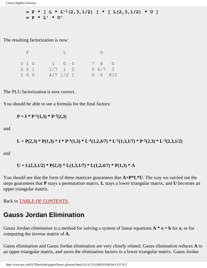
Linear Algebra Glossary
= P * [ L * L-1(2,3,1/2) ] * [ L(2,3,1/2) * U ] = P * L' * U'
The resulting factorization is now:
P L U
0 1 0 1 0 0 7 8 0 0 0 1 1/7 1 0 0 6/7 3 1 0 0 4/7 1/2 1 0 0 9/2
The PLU factorization is now correct.
You should be able to see a formula for the final factors:
P = I * P-1(1,3) * P-1(2,3)
and
L = P(2,3) * P(1,3) * I * P-1(1,3) * L-1(1,2,4/7) * L-1(1,3,1/7) * P-1(2,3) * L-1(2,3,1/2)
and
U = L(2,3,1/2) * P(2,3) * L(1,3,1/7) * L(1,2,4/7) * P(1,3) * A
You should see that the form of these matrices guarantees that A=P*L*U. The way we carried out the steps guarantees that P stays a permutation matrix, L stays a lower triangular matrix, and U becomes an upper triangular matrix.
Back to TABLE OF CONTENTS.
Gauss Jordan Elimination
Gauss Jordan elimination is a method for solving a system of linear equations A * x = b for x, or for computing the inverse matrix of A.
Gauss elimination and Gauss Jordan elimination are very closely related. Gauss elimination reduces A to an upper triangular matrix, and saves the elimination factors in a lower triangular matrix. Gauss Jordan
http://www.psc.edu/%7Eburkardt/papers/linear_glossary.html (53 of 151)2005/03/08 04:13:37 Þ.Ù

Linear Algebra Glossary
elimination proceeds relentlessly until A has been converted into the identity matrix.
Thus, unlike the Gauss elimination procedure, the Gauss Jordan elimination does not produce a factorization of the matrix, but only a solution to the linear system. This means that if a second linear system has to be solved, the matrix has to be set up and eliminated all over again.
The simplest way to describe Gauss Jordan is to note that to solve, say, the linear system A * x = b, the right hand side is appended as an extra column of the matrix. Then, on step I of the elimination, we choose a pivot row, move it to row I, divide it through by the pivot value, and then eliminate the matrix entries in column I from all other rows, rather than simply from rows I+1 through N. When the process is completed, the solution x has overwritten the right hand side b that was stored in column N+1.
Several right hand sides can be handled at once, by appending all of them to the coefficient matrix; the inverse can be computed by appending a copy of the identity matrix to the coefficient matrix before beginning elimination.
Gauss Jordan elimination is primarily used as a teaching tool, and for small linear systems. In practical computation, standard Gauss elimination is universally preferred.
Back to TABLE OF CONTENTS.
Gauss Seidel Iteration For Linear Equations
The Gauss Seidel iteration for linear equations is an iterative method for solving linear systems of equations A*x=b. It is similar to the the Jacobi algorithm and the successive overrelaxation method (SOR).
The Gauss Seidel iteration should only be used for matrices which are symmetric and positive definite, or for a matrix which is strictly diagonally dominant.
Each step of the Gauss Seidel iteration begins with an approximate answer x, and produces a new approximation y. Each component of y is computed in order, using the formula:
y(i) = [ b(i) - a(i,1)*y(1) - a(i,2)*y(2) ... - a(i,i-1)*y(i-1) - a(i,i+1)*x(i+1) ... - a(i,n)*x(n) ] / a(i,i)
http://www.psc.edu/%7Eburkardt/papers/linear_glossary.html (54 of 151)2005/03/08 04:13:37 Þ.Ù

Linear Algebra Glossary
The calculation of each entry of y is dependent on the calculation of the entries of lower index. Thus, the value of y(1) is calculated first, and then y(2) is calculated based on the values of y(1) as well as x(3) through x(n), and so on.
The process is to be repeated until the residual error is small, or the change in the approximate solution is negligible.
The Gauss Seidel iteration can be considered in terms of its matrix splitting. That is, if we decompose the matrix A into its strictly lower triangular, diagonal, and strictly upper triangular parts:
A = L + D + U
then the method is equivalent to the iteration
( L + D ) * xnew = b - U * x.
which means that the convergence of the algorithm can be understood in terms of the behavior of powers of the iteration matrix:
- ( L + D )-1 * U,
which in turn may best be understood by looking at the eigenvalues.
If the original coefficient matrix A is symmetric, then it may be preferred to use the symmetric Gauss Seidel iteration or SGS. In this case, the iteration consists of pairs of Gauss Seidel steps. The odd steps are the same as the usual iteration. But in the even steps, the variables are solved for in reverse order. Each pair of such steps is a single step of the SGS iteration, which has the property that its iteration matrix is similar to a symmetric matrix (though not necessarily symmetric itself). Among other things, this means that SGS can be used as a preconditioner for certain other problems.
Back to TABLE OF CONTENTS.
General Matrix Storage
A general matrix is one which has no special matrix structure or matrix symmetry.
In such a case, there are no space advantages to be gained by using a special matrix storage format, and so the matrix entries are stored using the standard two dimensional array format provided by the
http://www.psc.edu/%7Eburkardt/papers/linear_glossary.html (55 of 151)2005/03/08 04:13:37 Þ.Ù
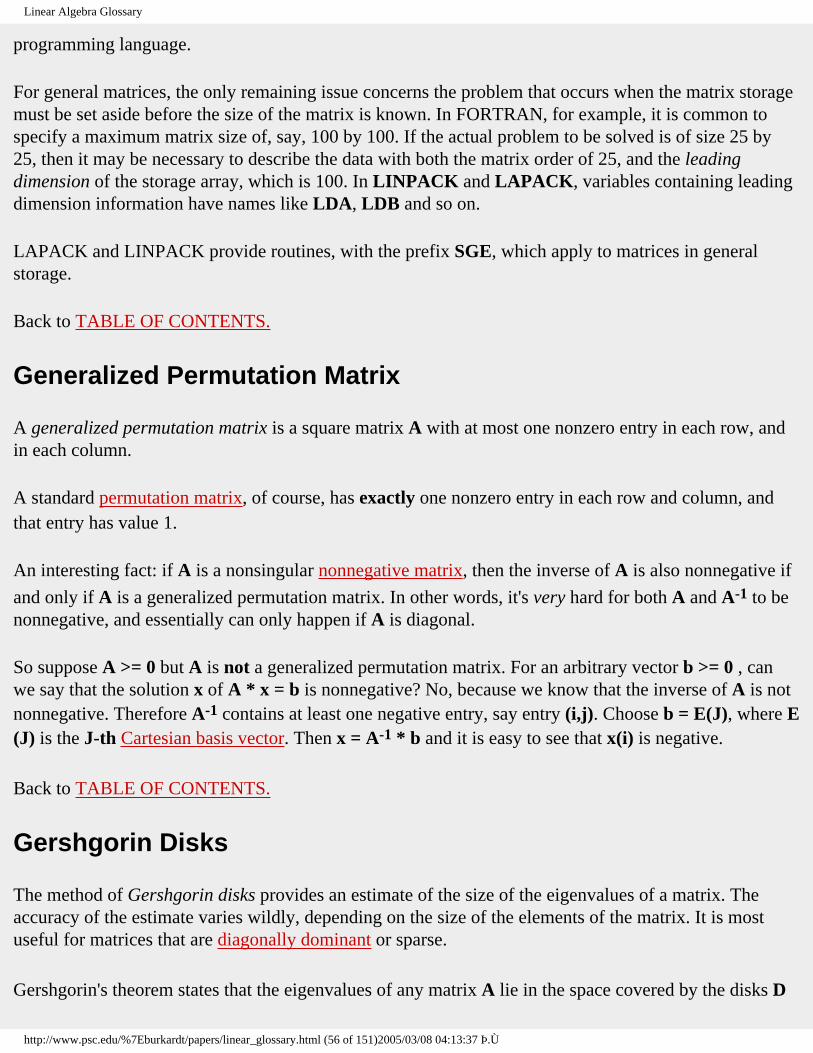
Linear Algebra Glossary
programming language.
For general matrices, the only remaining issue concerns the problem that occurs when the matrix storage must be set aside before the size of the matrix is known. In FORTRAN, for example, it is common to specify a maximum matrix size of, say, 100 by 100. If the actual problem to be solved is of size 25 by 25, then it may be necessary to describe the data with both the matrix order of 25, and the leading dimension of the storage array, which is 100. In LINPACK and LAPACK, variables containing leading dimension information have names like LDA, LDB and so on.
LAPACK and LINPACK provide routines, with the prefix SGE, which apply to matrices in general storage.
Back to TABLE OF CONTENTS.
Generalized Permutation Matrix
A generalized permutation matrix is a square matrix A with at most one nonzero entry in each row, and in each column.
A standard permutation matrix, of course, has exactly one nonzero entry in each row and column, and that entry has value 1.
An interesting fact: if A is a nonsingular nonnegative matrix, then the inverse of A is also nonnegative if
and only if A is a generalized permutation matrix. In other words, it's very hard for both A and A-1 to be nonnegative, and essentially can only happen if A is diagonal.
So suppose A >= 0 but A is not a generalized permutation matrix. For an arbitrary vector b >= 0 , can we say that the solution x of A * x = b is nonnegative? No, because we know that the inverse of A is not nonnegative. Therefore A-1 contains at least one negative entry, say entry (i,j). Choose b = E(J), where E(J) is the J-th Cartesian basis vector. Then x = A-1 * b and it is easy to see that x(i) is negative.
Back to TABLE OF CONTENTS.
Gershgorin Disks
The method of Gershgorin disks provides an estimate of the size of the eigenvalues of a matrix. The accuracy of the estimate varies wildly, depending on the size of the elements of the matrix. It is most useful for matrices that are diagonally dominant or sparse.
Gershgorin's theorem states that the eigenvalues of any matrix A lie in the space covered by the disks D
http://www.psc.edu/%7Eburkardt/papers/linear_glossary.html (56 of 151)2005/03/08 04:13:37 Þ.Ù

Linear Algebra Glossary
(I):
D(I) = ( x: sqrt ( x - A(I,I) )2 <= R(I) )
where R(I) is the sum of the absolute values of the off-diagonal elements of row I:
R(I) = sum ( J =/= I ) | A(I,J) |.
The theorem may also be applied using columns instead of rows.
Back to TABLE OF CONTENTS.
Givens Rotation Matrix
A Givens rotation is a linear transformation applied to two vectors, or two rows or columns of a matrix, which can be interpreted as a coordinate axis rotation. The intent of the rotation is to zero out an entry of the vector or matrix using an orthogonal transformation.
A Givens rotation is similar to the elementary row operation that adds a multiple of one row to another, but because a Givens rotation is an orthogonal similarity transformation, it offers greater stability and easy invertibility.
A Givens rotation matrix G has the form:
1 0 0 0 0 0 0 c 0 0 s 0 <-- row i 0 0 1 0 0 0 0 0 0 1 0 0 0 -s 0 0 c 0 <-- row j 0 0 0 0 0 1 ^ ^ col i col j
where c = cosine(theta) and s = sin(theta) for some angle theta.
Premultiplying A by G has the following effect:
row i of A is replaced by c*row i + s*row j in G*A; row j of A is replaced by -s*row i + c*row j in G*A.
http://www.psc.edu/%7Eburkardt/papers/linear_glossary.html (57 of 151)2005/03/08 04:13:37 Þ.Ù

Linear Algebra Glossary
while postmultiplication, A*G, would carry out a similar operation on the columns of A.
As an example, to zero out entry A(I,J) of a matrix requires a Givens rotation with values of cosine and sine so that:
- s * A(I,I) + c * A(I,J) = 0.
It's not actually necessary to compute the underlying rotation angle theta, since c and s can be computed directly:
s = A(I,J) / sqrt ( A(I,J)2 + A(I,I)2 ) c = A(I,I) / sqrt ( A(I,J)2 + A(I,I)2 )
For instance, to zero out the 3,1 entry of this matrix:
4 2 0 0 4 5 3 8 1
the sine and cosine are 3/5, 4/5, yielding a Givens matrix G of:
0.8 0 0.6 0 1 0 -0.6 0 0.8
and the product G * A:
5.0 6.4 6.0 0 4 5 0 5.2 8.0
It is possible to zero out entries of a matrix, one by one, using Givens rotations, similar to the way that Householder matrices are used, to reduce a matrix to a simpler form. The process can be used to zero out the entire lower triangle of a matrix, but further operations on the upper triangle would reintroduce zeroes in the lower triangle. Nonetheless, zeroing out the lower triangle means that Givens rotations can be used to produce the QR factorization of the matrix.
http://www.psc.edu/%7Eburkardt/papers/linear_glossary.html (58 of 151)2005/03/08 04:13:37 Þ.Ù

Linear Algebra Glossary
Back to TABLE OF CONTENTS.
Gram Schmidt Orthogonalization
Gram Schmidt orthogonalization is a process which starts with a set of N vectors X(I), each with M components, and produces a set of N2 orthonormal vectors Y which span the linear space of the original vectors.
N2 is less than N if the vectors X(I) are linearly dependent, and equal to N if they are linearly independent. Thus, one use for the Gram Schmidt process is simply to determine if a set of vectors are linearly dependent; a second is to determine the dimension of the space spanned by a linearly dependent set.
The Gram Schmidt process may be defined iteratively:
for I = 1 to N
N2 = I
Y(I) = X(I)
for J = 1 to I-1 C(J) = dot_product ( X(I), Y(J) ) Y(I) = Y(I) - C(J) * Y(J) end for
Norm = sqrt ( dot_product ( Y(I), Y(I) ) )
if ( Norm = 0 ) exit Y(I) = Y(I) / Norm
end for
Another way of looking at the process is to use the vectors to form the columns of a matrix A. The Gram Schmidt process can then be used to construct one version of the QR factorization of the matrix A:
A = Q * R
where Q is orthogonal and R is upper triangular.
http://www.psc.edu/%7Eburkardt/papers/linear_glossary.html (59 of 151)2005/03/08 04:13:37 Þ.Ù

Linear Algebra Glossary
Back to TABLE OF CONTENTS.
Hadamard Product
The Hadamard product of matrices A and B is a matrix C created by elementwise multiplication:
Ci,j = Ai,j * Bi,j
The Hadamard product is defined for any pair of rectangular matrices, as long as they have the same "shape", that is, the same number of rows, and the same number of columns.
Example of a Hadamard product:
1 2 3 * 7 8 9 = 7 16 27 4 5 6 10 11 12 40 55 72
Back to TABLE OF CONTENTS.
Hadamard's Inequality
Hadamard's inequality provides an upper bound on the size of the determinant of a matrix. It is related to the fact that the determinant represents the volume of an N-dimensional parallelepiped.
Let ||C(I)|| designate the Euclidean norm of column I of the matrix A. Hadamard's inequality states that
det ( A ) <= ||C(1)|| * ||C(2)|| * ... * ||C(N)||,
with equality holding only if one of the C(I)'s is zero, (yielding the minimum possible value of 0), or if all the C(I)'s are orthogonal (yielding the largest possible value).
The theorem may also be applied using rows instead of columns.
Back to TABLE OF CONTENTS.
Hankel Matrix
A Hankel matrix is a matrix which is constant along each of its anti-diagonals.
http://www.psc.edu/%7Eburkardt/papers/linear_glossary.html (60 of 151)2005/03/08 04:13:37 Þ.Ù

Linear Algebra Glossary
Here is an example of a square Hankel matrix:
7 6 5 4 6 5 4 3 5 4 3 2 4 3 2 1
and a rectangular Hankel matrix:
7 6 5 4 3 2 6 5 4 3 2 1 5 4 3 2 1 0
Simple facts about a Hankel matrix A:
● A is symmetric; ● the inverse of A is symmetric, but need not be a Hankel matrix;
Compare the concepts of Toeplitz Matrix, an Anticirculant Matrix, and a Persymmetric Matrix.
Back to TABLE OF CONTENTS.
Harwell Boeing Sparse Matrix Collection (HBSMC)
The Harwell Boeing Sparse Matrix Collection, or HBSMC, is a set of 43 data files describing a standard set of test sparse matrices for sparse matrix calculations.
The test set comprises linear systems, least squares problems, and eigenvalue calculations from a wide variety of disciplines. The set is offered as a standard benchmark for comparison of algorithms.
Here is an overview of the source and size of the various matrices:
Discipline Number Largest Largest number of order of nonzeroes matrices Counter examples, small matrices 3 11 76 Original Harwell test set 36 822 4841 Air traffic control 1 2873 15032
http://www.psc.edu/%7Eburkardt/papers/linear_glossary.html (61 of 151)2005/03/08 04:13:37 Þ.Ù

Linear Algebra Glossary
Astrophysics 2 765 24382 Chemical Engineering 16 2021 7353 Circuit simulation 1 991 6027 Demography 3 3140 543162 Economic modelling 11 2529 90158 Nuclear reactor core modelling 3 1374 8606 Optimal power flow problems 3 4929 47369 Stochastic modelling 7 1107 5664 Acoustic scattering 4 841 4089 Oil reservoir modelling 19 5005 20033 Stiff ODE problems 10 760 5976 George and Liu test problems 21 3466 13681 Model PDE problems 3 900 4322 Navier Stokes problems 7 3937 25407 Unassembled finite element matrices 10 5976 15680 Oceanography 4 1919 17159 Power network matrices 14 5300 13571 Everstine test set, ship structures 30 2680 23853 Structures, eigenproblems 22 15439 133840 Structures, linear equations 36 44609 1029655 Least squares problems 4 1850 10608
The SPARSKIT package includes utilities for conversion of matrices in the Harwell Boeing format into other formats, such as that used by ELLPACK and ITPACK.
Back to TABLE OF CONTENTS.
HBSMC Sparse Matrix Storage
The Harwell Boeing Sparse Matrix Collection uses a matrix storage format which is a special kind of sparse matrix storage for most of the matrices in the collection.
The standard sparse matrix format is column oriented. That is, the matrix is represented by a sequence of columns. Each column is held as a sparse vector, represented by a list of row indices of the entries in an integer array and a list of the corresponding values in a separate real array. A single integer array and a single real array are used to store the row indices and the values, respectively, for all the columns.
Data for each column are stored in consecutive locations. The columns are stored in order, and there is no space between columns. A separate integer array holds the location of the first entry of each column, and the first free location. For symmetric and Hermitian matrices, only the entries of the lower triangle are stored, including the diagonal. For antisymmetric matrices, only the strict lower triangle is stored.
http://www.psc.edu/%7Eburkardt/papers/linear_glossary.html (62 of 151)2005/03/08 04:13:37 Þ.Ù

Linear Algebra Glossary
Here is a simple example of a 5 by 5 matrix:
1.0 -3.0 0.0 -1.0 0.0 0.0 0.0 -2.0 0.0 3.0 2.0 0.0 0.0 0.0 0.0 0.0 4.0 0.0 -4.0 0.0 5.0 0.0 -5.0 0.0 6.0
This matrix would be stored in the arrays
● COLPTR (location of the first entry of a column), ● ROWIND (row indices) and ● VALUES (numerical values)
as follows:
Subscripts: 1 2 3 4 5 6 7 8 9 10 11
COLPTR 1 4 6 8 10 12 ROWIND 1 3 5 1 4 2 5 1 4 2 5 VALUES 1.0 2.0 5.0 -3.0 4.0 -2.0 -5.0 -1.0 -4.0 3.0 6.0
We can generate column 5, say, by observing that its first entry is in position COLPTR(5)=10 of arrays ROWIND and VALUES. This entry is in row ROWIND(10)=2 and has value VALUES(10)=3.0. Other entries in column 5 are found by scanning ROWIND and VALUES to position COLPTR(6)-1, that is, position 11. Thus, the only other entry in column 5 is in row ROWIND(11)=5 with value VALUES(11)=6.
Back to TABLE OF CONTENTS.
HBSMC Finite Element Matrix Storage
The HBSMC finite element storage format is a special matrix storage format for those matrices in the collection which derive from a finite element problem.
Matrices arising in finite element applications are usually assembled from numerous small elemental matrices. The collection includes a few sparse matrices in original unassembled form. The storage of the individual unassembled matrices is based on the general sparse format, which stores a matrix as a list of
http://www.psc.edu/%7Eburkardt/papers/linear_glossary.html (63 of 151)2005/03/08 04:13:37 Þ.Ù

Linear Algebra Glossary
matrix columns. The elemental representation stores the matrix as a list of elemental matrices. Each elemental matrix is represented by a list of the row/column indices (variables) associated with the element and by a small dense matrix giving the numerical values by columns, or in the symmetric case, only the lower triangular part. The lists of indices are held contiguously, just as for the lists of row indices in the standard format. The dense matrices are held contiguously in a separate array, with each matrix held by columns. Although there is not a one to one correspondence between the arrays of integer and numerical values, the representation does not hold the pointers to the beginning of the real values for each element. These pointers can be created from the index start pointers (ELTPTR) after noting that an element with NU variables has NU*NU real values, or (NU*(NU+1))/2 in the symmetric case.
We illustrate the elemental storage scheme with a small, 5 by 5 example:
5.0 0.0 0.0 1.0 2.0 0.0 4.0 3.0 0.0 6.0 0.0 3.0 7.0 8.0 1.0 1.0 0.0 8.0 9.0 0.0 2.0 6.0 1.0 0.0 10.0
generated from four elemental matrices:
1 4 1 5 2 3 5 3 4 1 (2.0 1.0) 1 (3.0 2.0) 2 (4.0 3.0 6.0) 3 (2.0 8.0) 4 (1.0 7.0) 5 (2.0 8.0) 3 (3.0 5.0 1.0) 4 (8.0 2.0) 5 (6.0 1.0 2.0)
where the variable indices are indicated by the integers marking the rows and columns. This matrix would be stored in the ELTPTR (location of first entry), VARIND (variable indices) and VALUES (numerical values) arrays as follows:
Subscripts: 1 2 3 4 5 6 7 8 9 10 11 12 13 14 15 ELTPTR: 1 3 5 8 10 VARIND: 1 4 1 5 2 3 5 3 4 VALUES: 2. 1. 7. 3. 2. 8. 4. 3. 6. 5. 1. 2. 2. 8. 2.
Back to TABLE OF CONTENTS.
http://www.psc.edu/%7Eburkardt/papers/linear_glossary.html (64 of 151)2005/03/08 04:13:37 Þ.Ù

Linear Algebra Glossary
Hermite Normal Form
A nonsingular integer matrix is in Hermite Normal Form if it is lower triangular, all entries are non-negative, and each row has a unique maximum element which is located on the main diagonal.
(In some definitions, the matrix is required to be upper triangular instead.)
Any nonsingular integer matrix can be transformed to Hermite Normal Form using a series of unimodular column operations:
● add an integer multiple of one column to another; ● exchange two columns; ● multiple any column by -1.
For example, given the matrix A:
5 2 1 -4 2 4 0 -3 6
its Hermite normal form is:
1 0 0 4 6 0 6 15 30
Back to TABLE OF CONTENTS.
Hermitian Matrix
A Hermitian matrix A is a complex matrix that is equal to its complex conjugate transpose:
A = AH
Here is a Hermitian matrix:
1 1+2i 3-4i 1-2i 4 6i 3+4i -6i 8
http://www.psc.edu/%7Eburkardt/papers/linear_glossary.html (65 of 151)2005/03/08 04:13:37 Þ.Ù

Linear Algebra Glossary
Simple facts about a Hermitian matrix A:
● The diagonal entries of A must be real. ● The eigenvalues of A are real, although the eigenvectors are generally complex. ● Eigenvectors of A that correspond to different eigenvectors will be orthogonal. ● A can be decomposed into the form A = U*LAMBDA*UH where U is unitary and LAMBDA is
real and diagonal.
The corresponding concept for real matrices is symmetric.
Back to TABLE OF CONTENTS.
Hessenberg Matrix
An upper Hessenberg matrix is a matrix which is entirely zero below the first subdiagonal.
An upper Hessenberg matrix is "almost" upper triangular. A lower Hessenberg matrix is, of course, entirely zero above the first superdiagonal. Upper Hessenberg matrices occur so often that they are frequently simply called "Hessenberg" matrices.
An example of an upper Hessenberg matrix is:
1 2 3 4 5 6 7 8 9 1 0 5 4 3 2 0 0 8 3 7 0 0 0 9 1
Eigenvalue programs typically transform a matrix into upper Hessenberg form, and then carry out the QR method on this matrix, which converges rapidly to a matrix which is diagonal except for 2 by 2 blocks corresponding to complex eigenvalues.
The reason for transforming a matrix into upper Hessenberg form is that the QR method is much less expensive if carried out on an upper Hessenberg matrix. It is actually cheaper to go to the additional trouble of transforming a matrix to upper Hessenberg form, and then carrying out the QR method on that matrix, rather than carrying out the QR method on the original matrix.
Back to TABLE OF CONTENTS.
http://www.psc.edu/%7Eburkardt/papers/linear_glossary.html (66 of 151)2005/03/08 04:13:37 Þ.Ù

Linear Algebra Glossary
Householder Matrix
A Householder matrix for a given vector v has the form:
H = I - 2 * v * vT / ( norm2 ( v ) )2
or, in the common case where the Euclidean norm of v is 1, we may write:
H = I - 2 * v * vT
For the simple case where w = (1/3, 2/3, 2/3), here is what H would look like:
(1 0 0) (1/9 2/9 2/9) ( 7/9 -4/9 -4/9) (0 1 0) - 2 * (2/9 4/9 4/9) = (-4/9 1/9 -8/9) (0 0 1) (2/9 4/9 4/9) (-4/9 -8/9 1/9)
A little "reflection" will convince you that the Householder matrix for any vector v will always be symmetric, just like this example.
The Householder matrix is also orthogonal:
H * HT = H * H = I.
Householder matrices can be used to compute the QR factorization of a matrix. A Householder matrix can be found which will "wipe out" all the subdiagonal entries of the first column of the original matrix. Another Householder matrix can be found which will "wipe out" all the subdiagonal entries of the second column, and so on. At the end of N-1 steps of this process, we have computed
Hn-1 * ... * H2 * H1 * A = R
where R is upper triangular. But the product
H = Hn-1 * ... * H2 * H1
is an orthogonal matrix. We can multiply both sides by its transpose, which is also its inverse, to get
A = HT * R
http://www.psc.edu/%7Eburkardt/papers/linear_glossary.html (67 of 151)2005/03/08 04:13:37 Þ.Ù

Linear Algebra Glossary
or, if we define Q to be HT:
A = Q * R.
The Householder matrix is sometimes called an elementary reflector.
Back to TABLE OF CONTENTS.
Idempotent Matrix
An idempotent matrix A has the property that
A * A = A
An idempotent matrix is sometimes called a projector matrix.
Simple facts about an idempotent matrix A:
● The identity matrix is idempotent; ● Every point of the form A*x is a fixed point of A, that is A * ( A * x ) = A * x; ● If A is idempotent, and it is not the identity matrix, it must be singular; ● The only eigenvalues of A are 0 and 1; ● I-A is also idempotent; ● rank(A) = trace(A); ● I-2*A is involutory;
Back to TABLE OF CONTENTS.
The Identity Matrix
The identity matrix, usually denoted I, is a square matrix with 1's on the main diagonal and 0's elsewhere. The identity matrix behaves like the number 1 in matrix multiplication. For any matrix A:
A * I = I * A = A.
Here is the 3 by 3 identity matrix:
1 0 0 0 1 0 0 0 1
http://www.psc.edu/%7Eburkardt/papers/linear_glossary.html (68 of 151)2005/03/08 04:13:37 Þ.Ù

Linear Algebra Glossary
Simple facts about the identity matrix I:
● The norm of I must be 1, for any vector-bound matrix norm ● The condition number of I must be 1, for any vector-bound matrix norm;
● IT = I-1 = I; ● The eigenvalues of I are 1, with algebraic and geometric multiplicity N; ● Every nonzero vector x is an eigenvector of I. A basis for the eigenspace of I is the set of
columns of I. ● I is diagonal; ● I is idempotent; ● I is involutory; ● I is symmetric; ● I is an orthogonal projector;
Back to TABLE OF CONTENTS.
Ill Conditioned Linear System
When solving a linear system A * x = b, the matrix A is said to be ill conditioned if small errors or perturbations in the coefficient matrix A or right hand side b correspond to large errors or perturbations in the solution x.
A numerical scale for ill conditioning is provided by the condition number.
Linear systems which are extremely ill conditioned may be impossible to solve accurately. A standard example of an ill conditioned matrix is the Hilbert Matrix, with A(I,J) = 1 / ( I + J ).
Back to TABLE OF CONTENTS.
The Incomplete LU factorization
The incomplete LU factorization is an approximate LU factorization of a matrix A, comprising a unit lower triangular matrix L and an upper triangular matrix U.
Typically, the matrix A is large and sparse, and an iterative scheme is being used to solve the linear system A*x=b. The incomplete LU factorization is intended as a preconditioner, which modifies the linear system, improving the convergence rate of the iterative scheme. In particular, the preconditioner matrix is M=L*U, and we are well advised to store L and U instead of M, since this gives us an easy
http://www.psc.edu/%7Eburkardt/papers/linear_glossary.html (69 of 151)2005/03/08 04:13:37 Þ.Ù

Linear Algebra Glossary
way of solving linear systems associated with M.
The computation of the incomplete LU factorization is similar to that of the usual PLU factors except for two points. First, we assume that no pivoting is required, hence the P factor can be omitted. Secondly, if the original matrix A has a zero entry, then we require that the corresponding entry of the U matrix be zero. This means that there is no fill in (and it is also why L*U will not equal A). Because there is no fill in, the factors L and U can actually be stored in a data structure that is the same as that of A. The elements of L are stored in the positions devoted to lower triangular elements of A, while U goes in the diagonal and upper triangular locations.
Back to TABLE OF CONTENTS.
Inertia
The oddly named inertia of a (square) matrix is the numbers of negative, zero, and positive eigenvalues.
Sylvester's Law of Inertia states that if A and B are congruent matrices, then we cannot guarantee that they have the same eigenvalues, but they do have the same inertias.
This theorem allows us to determine if a symmetric matrix is positive definite. Because the matrix is symmetric, we can compute an LDL factorization:
A = L * D * LT
where L is unit lower triangular, and D is diagonal. This means that A is congruent to the diagonal matrix D. But the eigenvalues of D are easily determined, from which we can get the inertia of D. This is equal to the inertia of A; in particular, if D has only positive eigenvalues, then so does A, which is therefore positive definite.
Moreover, if such a factorization is cheap, as for a tridiagonal symmetric matrix, then we can search for eigenvalues by seeking diagonal shifts of the matrix that cause the number of negative eigenvalues to change by 1.
Back to TABLE OF CONTENTS.
Inner Product
An inner product is a scalar-valued function of two vectors x and y, denoted (x,y), with the properties that:
http://www.psc.edu/%7Eburkardt/papers/linear_glossary.html (70 of 151)2005/03/08 04:13:37 Þ.Ù

Linear Algebra Glossary
● ( x, y ) = ( y, x ), symmetry ● ( x, s * y ) = s * ( x, y ) for any scalar s, linearity ● ( x, y + z ) = ( x, y ) + ( x, z ) additivity ● ( x, x ) >= 0, and equal to zero only if x = 0, positivity. ● ( x, A * y ) = ( AT * x, y ).
A vector inner product (x,y) can be used to define a corresponding vector norm ||x||:
|| x || = sqrt ( x, x ).
If the inner product and norm are related in this way, then the Cauchy-Schwarz inequality relates them.
The inner product is sometimes referred to as the dot product (because it is often represented as x dot y), or as the scalar product (because its result is a scalar value).
Back to TABLE OF CONTENTS.
Inverse Matrix
The inverse matrix of a square matrix A, if it exists, is a matrix denoted A-1 with the property that
A * A-1 = A-1 * A = I.
If the inverse matrix exists, it is unique, and A is said to be nonsingular or invertible. Otherwise, A is singular.
If the inverse of A exists, then the solution of
A * x = b
can be immediately written down:
x = A-1 * b.
However, it's not a good idea to solve a linear system in this way. The inverse is relatively expensive to compute, and subject to greater inaccuracies than other solution methods. This is not to say that the inverse isn't useful. Orthogonal and unitary transformations are so popular in numerical linear algebra because their inverses "come for free"; (and their inverses are very well conditioned).
Simple facts:
http://www.psc.edu/%7Eburkardt/papers/linear_glossary.html (71 of 151)2005/03/08 04:13:37 Þ.Ù

Linear Algebra Glossary
● if lambda is an eigenvalue of A, then 1/lambda is an eigenvalue of A-1; ● if x is an eigenvector of A, x is also an eigenvector of A-1.
LAPACK and LINPACK include routines for explicitly computing the inverse of a given matrix.
Back to TABLE OF CONTENTS.
Inverse Power Method
The inverse power method is a technique for solving the eigenvalue problem.
The inverse power method is related to the power method, but is more flexible. Through the use of shifts, it can be "aimed" to seek the eigenvalue that is closest to any particular target value. Moreover, once a rough estimate of an eigenvalue is made, the shift can be set to this value, which will increase the convergence rate of the algorithm.
The inverse power method only requires that the user be able to repeatedly solve linear systems of the form:
A * x = b
or, when shifts are used,
( A - shift * I ) * x = b.
Thus, for instance, if A is a band matrix or a sparse matrix, the user can employ a storage method and solution algorithm appropriate to the particular form of the problem.
The inverse power method gets its name from the fact that, when the shift is zero, it is equivalent to using the power method on the matrix A-1.
The inverse power method begins by picking a starting guess for the eigenvector x, and the eigenvalue lambda. If the shift will not vary then a fixed value should be set now. Then repeat the following steps as often as necessary:
● Set norm = the norm of x; ● Set x = x / norm; ● Set lambda_Old = lambda; ● Set lambda = 1 / norm; ● If the shift may vary, set shift = lambda;
http://www.psc.edu/%7Eburkardt/papers/linear_glossary.html (72 of 151)2005/03/08 04:13:37 Þ.Ù

Linear Algebra Glossary
● Solve ( A - shift * I ) * xnew = x. ● If no convergence, set xnew = x and repeat.
Back to TABLE OF CONTENTS.
Invertible Matrix
An invertible matrix A is a (square) matrix for which there exists an inverse matrix B, called the inverse of A.
A square matrix A is invertible if and only if:
● no eigenvalue of A is zero; ● no singular value of A is zero; ● every linear system A * x = b has a unique solution; ● the null space of A is exactly the zero vector; ● the rows (and the columns) of A are linearly independent; ● the determinant of A is nonzero; ● Gauss elimination, with partial pivoting, and exact arithmetic, never encounters a zero pivot
(including the "unused" pivot on the last step).
Back to TABLE OF CONTENTS.
Involutory Matrix
An involutory matrix A has the property that
A * A = I.
Simple facts about an involutory matrix A:
● The identity matrix is involutory; ● A is invertible, and A-1=A;
Back to TABLE OF CONTENTS.
Irreducible Matrix
An irreducible matrix is a (square) matrix which is not reducible.
http://www.psc.edu/%7Eburkardt/papers/linear_glossary.html (73 of 151)2005/03/08 04:13:37 Þ.Ù

Linear Algebra Glossary
Definition One: A reducible matrix is one which can be rearranged into the following block form:
( P Q ) ( 0 R )
where P and R are square sub-blocks, and "0" represents a (nonempty) rectangular block of zero entries. The rearrangement can be done by simultaneous row and column permutations. An irreducible matrix is one which is not reducible.
Definition Two: A matrix is irreducible if and only if, for any row index i and column index j, there is always a nonnegative integer p (which may be 0) and a sequence of integers k1, ..., kp so that the product
Ai,k1 * Ak1,k2 * ... * Akp,j
is nonzero.
Definition Three: A nonnegative matrix A is irreducible if and only if, for any vector x>0 it is the case that A*x>0.
Definition Two implies that if the entries of A are nonnegative, then all entries of AN-1 are positive except for the diagonal entries which may be zero. (This has implications for the use of the power method.)
Definition Three: A matrix of order N is irreducible if, for any division of the integers between 1 and N into two disjoint sets K1 and K2, there is always a nonzero element A(I,J) with I in K1 and J in K2.
The concept of an irreducible matrix is mainly of interest in the analysis of the convergence of certain iterative schemes for linear equations. One key idea is the following: if the matrix A is irreducible and diagonally dominant, then A is nonsingular.
If you only know that the matrix is diagonally dominant, then Gershgorin's theorem would still not rule out an eigenvalue of zero, and hence singularity. It's the irreducibility that guarantees no zero eigenvalue here. The "1, -2, 1" tridiagonal matrix is an example where this theorem applies.
Here's an example of an irreducible matrix with zero main diagonal:
0 1 0 0 1 0 1 0 0 1 0 1
http://www.psc.edu/%7Eburkardt/papers/linear_glossary.html (74 of 151)2005/03/08 04:13:37 Þ.Ù

Linear Algebra Glossary
0 0 1 0
If you're familiar with graph theory, then a matrix A is irreducible if and only if the digraph with corresponding adjacency matrix is strongly connected. (Consider node I to be connected to node J if A(I,J) is nonzero. The digraph is strongly connected if you can get from any node to any other node following directed edges.)
Back to TABLE OF CONTENTS.
Iterative Methods for Eigenvalues
A method is called iterative when it consists of a basic series of operations which are carried out over and over again, until the answer that is produced is no longer significantly changing, or some exceptional error occurs, or the limit on the number of steps is exceeded.
All eigenvalue problems are solved by iterative methods, except for the "toy" problems presented in textbooks. This is because the computation of eigenvalues is equivalent to finding the roots of a polynomial, and there is no explicit method for finding the roots of a general polynomial of degree 5 or higher.
The best known methods for the eigenvalue problem include:
● the power method; ● the inverse power method; ● the Jacobi Algorithm; ● the QR method.
Back to TABLE OF CONTENTS.
Iterative Methods for Linear Equations
A method is called iterative when it consists of a basic series of operations which are carried out over and over again, until the answer that is produced is no longer significantly changing, or some exceptional error occurs, or the limit on the number of steps is exceeded.
A direct method is the "opposite" of an iterative method. A fixed number of operations are carried out once, at the end of which the solution is produced. Gauss elimination on a linear system is an example of such a direct method. Direct methods are the primary method for solving small or dense or nonsymmetric linear systems.
http://www.psc.edu/%7Eburkardt/papers/linear_glossary.html (75 of 151)2005/03/08 04:13:37 Þ.Ù

Linear Algebra Glossary
The most common reason for using an iterative method is that it can require far less storage than a direct method. An iterative method typically only sets aside storage for the original nonzero entries of the matrix; no fill in occurs. Standard direct methods must set aside an entry for every possible position in the matrix, though some reduction in this requirement is possible if the matrix is banded.
Secondly, each iteration typically takes much less time than a full direct solve; thus, it is possible, for some problems, that an iterative method will actually converge to an acceptable answer more quickly than a direct method.
An iterative method has numerous disadvantages. You will need a starting point, and if you pick a poor one that may slow down convergence. Your system matrix usually needs to satisfy extra conditions beyond merely being nonsingular. The rate of convergence may be extremely slow, although this can be helped by a suitable preconditioner. If you have a very large problem and are storing the matrix in a compact form, the programming and computational cost involved in storing and retrieving coefficient data can exceed that of the solution phase.
Iterative methods are generally only suitable for certain kinds of system matrices. The most common requirements are that the matrix be positive definite symmetric or strictly diagonally dominant.
Iterative methods for solving systems of linear equations include:
● Gauss Seidel Iteration;; ● the Jacobi Algorithm ; ● the conjugate gradient method; ● Successive Overrelaxation Method (SOR).
Back to TABLE OF CONTENTS.
Iterative Refinement
Iterative refinement is an attempt to "improve" a computed solution x0 for the linear system of equations A*x=b.
The algorithm is occasionally effective when the coefficient matrix is ill conditioned, a problem that may become evident if the residual error is computed, and seen to be relatively large.
A single step of the algorithm involves computing the residual error:
r := b - A * x,
http://www.psc.edu/%7Eburkardt/papers/linear_glossary.html (76 of 151)2005/03/08 04:13:37 Þ.Ù

Linear Algebra Glossary
solving the linear system:
A * dx = r,
and adding the correction dx to the original solution x.
x := x + dx.
In order to achieve any improvement in accuracy, the residual error should be calculated in higher arithmetic precision. The rest of the calculation can be done in single precision, allowing the use of the already computed LU factorization of A, if available. However, to compute the residual error, the original matrix A is needed. It is preferable to figure out how to use the LU factors to compute the residual error, rather than keeping two copies of the matrix, one factored and one untouched.
If the residual error of the new solution is still too large, but somewhat better, then the procedure may be repeated as often as desired.
A subroutine SGEIM for carrying out iterative refinement using the LINPACK routines is described in the LINPACK User's Guide.
Back to TABLE OF CONTENTS.
Jacobi Algorithm for Eigenvalues
The Jacobi algorithm for computing eigenvalues is an iterative method, which may be applied to a symmetric matrix A, to compute its eigenvalues and eigenvectors.
The method will produce an orthogonal matrix Q and an "approximately" diagonal matrix lambda such that
A = QT * lambda * Q.
The steps of the iteration compute a sequence of orthogonal matrices Q1, Q2, ... which transform the original matrix A into matrices A1, A2, ... each of which has the same eigenvalues as A, but each of which is "more" diagonal than A was. Starting with A, we determine Q1, and produce A1, which is orthogonally similar to A:
A1 = Q1T * A * Q1.
We then determine a matrix Q2 that produces A2:
http://www.psc.edu/%7Eburkardt/papers/linear_glossary.html (77 of 151)2005/03/08 04:13:37 Þ.Ù

Linear Algebra Glossary
A2 = Q2T * A1 * Q2 = ( Q1 * Q2 )T * A * ( Q1 * Q2 ).
The point of the algorithm is how we choose the matrices Q at each step. Q1 is chosen in such a way as to "annihilate" the (1,2) and (2,1) elements of A. That is, the (1,2) and (2,1) elements of A1 will be zero. Q2 will eliminate the (1,3) and (3,1) elements of A1. Thus A2 will have zeroes in the (1,3) and (3,1) positions. Unfortunately, the (1,2) and (2,1) positions of A2, which we just zeroed out on the previous step, will not remain zero, but will fill in again! However, the fill in values are generally smaller than the original values. As we can sweep through the entire matrix, we repeatedly annihilate the off-diagonal elements until they all have decreased below some tolerance.
It can be shown that the sum of the squares of the off diagonal elements always decreases to zero with the iteration. Thus, for some iteration step M, one can expect to have a matrix AM and a matrix
Q = Q1*Q2*...*QM
so that
AM = QT * A * Q
where AM is "essentially" diagonal. At that point, we can rewrite this equation as
A * Q = lambda * Q
where lambda is the diagonal entries of AM, and is the eigenvalues of A, and the transformation matrix Q is the matrix of eigenvectors of A. Thus, if the off diagonal elements disappear as promised, we have approximately solved our eigenvalue problem.
So which orthogonal matrix Q zeroes out a specific pair of entries? The formula is fairly simple. To annihilate the arbitrary entries A(I,J) and A(J,I), the matrix Q is equal to the identity matrix, except for:
Q(I,I) = C Q(I,J) = S Q(J,I) = - S Q(J,J) = C
where C and S are the cosine and sine of some rotation angle THETA. Thus, each matrix Q is a Givens rotation matrix. We can compute C and S directly (skipping the computation of THETA) by the following formula:
http://www.psc.edu/%7Eburkardt/papers/linear_glossary.html (78 of 151)2005/03/08 04:13:37 Þ.Ù

Linear Algebra Glossary
U = ( A(J,J) - A(I,I) ) / ( 2 * A(I,J) ) T = sign ( U ) / ( | U | + sqrt ( U2 + 1 ) ) C = 1 / sqrt ( T2 + 1 ) S = T / sqrt ( T2 + 1 )
The Jacobi method is simple and easy to program, but is usually slower than the QR method.
Back to TABLE OF CONTENTS.
The Jacobi Algorithm for Linear Equations
The Jacobi algorithm for linear equations is an iterative method for solving linear systems of equations A * x = b.
The method is similar to the Gauss Seidel and Successive Overrelation Method (SOR), but has the distinction of being the only simple iterative method that is easy to program in parallel.
The Jacobi iteration is only appropriate for matrices which are strictly diagonally dominant or else symmetric and positive definite.
Each step of the Jacobi iteration begins with an approximate solution x. An improved approximate solution xnew is computed by solving N independent linear equations:
xnew(i) = [ b(i) - A(i,1) * x(1) - A(i,2) * x(2) ... - A(i,i-1) * x(i-1) - 0.0 * x(i) <-- note that we are skipping x(i) here! - A(i,i+1) * x(i+1) ... - A(i,n) * x(n) ] / A(i,i)
Once xnew is computed, the residual error is calculated:
r = A * xnew - b
http://www.psc.edu/%7Eburkardt/papers/linear_glossary.html (79 of 151)2005/03/08 04:13:37 Þ.Ù

Linear Algebra Glossary
and the solution increment:
dx = xnew - x.
If the norms of these vectors are satisfactorily small, the iteration may be halted. Otherwise, xnew becomes the new starting guess x for the next step of the iteration.
The Jacobi iteration can be considered in terms of its matrix splitting. That is, if we decompose the matrix A into its strictly lower triangular, diagonal, and strictly upper triangular parts:
A = L + D + U
then the method is equivalent to the iteration
D * xnew = b - ( L + U ) * x.
which means that the convergence of the algorithm can be understood in terms of the behavior of powers of the iteration matrix:
- D-1 * ( L + U ),
which in turn may best be understood by looking at the eigenvalues. Note that if A is symmetric, then so is the iteration matrix.
Back to TABLE OF CONTENTS.
The Jacobi Preconditioner
The Jacobi preconditioner is a very simple preconditioning matrix for use with an iterative method for linear equations.
For a given system matrix A, the Jacobi preconditioner matrix M is the diagonal matrix whose entries are defined by
M = diag ( A )
In effect, using the Jacobi preconditioner amounts to dividing each equation and right hand side entry by the corresponding diagonal entry of the original coefficient matrix.
Back to TABLE OF CONTENTS.
http://www.psc.edu/%7Eburkardt/papers/linear_glossary.html (80 of 151)2005/03/08 04:13:37 Þ.Ù

Linear Algebra Glossary
Jordan Canonical Form
The Jordan canonical form of a matrix A is an upper bidiagonal matrix whose main diagonal contains the eigenvalues of A, and whose superdiagonal contains only zeroes or ones. The location of the ones in the superdiagonal is determined by the algebraic and geometric multiplicity of the eigenvalues.
Here is an example of a Jordan canonical form:
4 0 0 0 0 0 2 1 0 0 0 0 2 1 0 0 0 0 2 0 0 0 0 0 3
Every matrix is unitarily similar to its Jordan Canonical Form. That is, for any matrix A, there exists a unitary matrix U so that
A = U* * J * U
where J has Jordan canonical form. This form can also be regarded as a matrix factorization.
If A is real, but has complex eigenvalues, the matrix J has complex entries.
The Jordan canonical form is of little interest to computational linear algebraists. Unless exact arithmetic is used, it is extremely sensitive to small errors, and the information it provides can be computed more reliably in other ways.
Back to TABLE OF CONTENTS.
L1 Matrix Norm
The L1 matrix norm is a matrix norm that is vector-bound to, and hence compatible with, the L1 vector norm.
Thus, the formal definition of the norm is
||A|| = max ( || A*x || / ||x|| )
http://www.psc.edu/%7Eburkardt/papers/linear_glossary.html (81 of 151)2005/03/08 04:13:37 Þ.Ù

Linear Algebra Glossary
where the vector norm used on the right hand side is the L1 vector norm, and the maximum is taken over all nonzero vectors x.
However, it is easy to show that the L1 matrix norm has a simpler formula: ||A|| = the maximum, over all matrix columns, of the sum of the absolute values of the entries in the column.
Back to TABLE OF CONTENTS.
L1 Vector Norm
The L1 vector norm is a vector norm defined as
||x|| = sum ( 1 <= I <= N ) |x(i)|.
Back to TABLE OF CONTENTS.
L2 Matrix Norm
The L2 matrix norm is a matrix norm that is vector-bound to, and hence compatible with, the L2 vector norm.
Thus, the formal definition of the norm is
||A|| = max ( || A*x || / ||x|| )
where the vector norm used on the right hand side is the L2 vector norm, and the maximum is taken over all nonzero vectors x.
The L2 matrix norm has another formulation: ||A|| = the square root of the maximum absolute value of the eigenvalues of AT * A.
The computation of the L2 norm is expensive, and so it is often simpler to use the easily-computed Frobenius matrix norm, which is not vector-bound to the L2 vector norm, but is compatible with it.
Back to TABLE OF CONTENTS.
L2 Vector Norm
The L2 vector norm is a vector norm defined as
http://www.psc.edu/%7Eburkardt/papers/linear_glossary.html (82 of 151)2005/03/08 04:13:37 Þ.Ù

Linear Algebra Glossary
||x|| = sqrt ( sum ( 1 <= I <= N ) x(i)2 )
The L2 vector norm is also known as the Euclidean vector norm or the root-mean-square vector norm.
Back to TABLE OF CONTENTS.
L Infinity Matrix Norm
The L Infinity matrix norm is a matrix norm that is vector-bound to, and hence compatible with, the L Infinity vector norm.
Thus, the formal definition of the norm is
||A|| = max ( || A*x || / ||x|| )
where the vector norm used on the right hand side is the L Infinity vector norm, and the maximum is taken over all nonzero vectors x.
However, it is easy to show that the L Infinity matrix norm has a simpler formula: ||A|| = the maximum, over all matrix rows, of the sum of the absolute values of the entries in the row.
Back to TABLE OF CONTENTS.
L Infinity Vector Norm
The L Infinity vector norm is a vector norm defined as
||x|| = max ( 1 <= I <= N ) |x(i)|.
Back to TABLE OF CONTENTS.
LAPACK
LAPACK is a set of linear algebra routines, intended as the replacement for LINPACK and EISPACK. It is a project sponsored by the Argonne National Laboratories and the Numerical Algorithms Group (NAG). The LAPACK routines are intended to achieve optimal performance on various machines by calling the level 3 BLAS, which use block methods to achieve high performance.
http://www.psc.edu/%7Eburkardt/papers/linear_glossary.html (83 of 151)2005/03/08 04:13:37 Þ.Ù
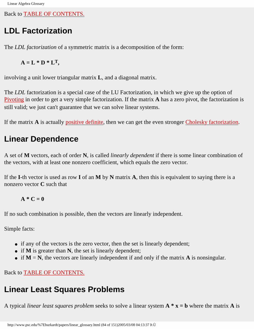
Linear Algebra Glossary
Back to TABLE OF CONTENTS.
LDL Factorization
The LDL factorization of a symmetric matrix is a decomposition of the form:
A = L * D * LT,
involving a unit lower triangular matrix L, and a diagonal matrix.
The LDL factorization is a special case of the LU Factorization, in which we give up the option of Pivoting in order to get a very simple factorization. If the matrix A has a zero pivot, the factorization is still valid; we just can't guarantee that we can solve linear systems.
If the matrix A is actually positive definite, then we can get the even stronger Cholesky factorization.
Linear Dependence
A set of M vectors, each of order N, is called linearly dependent if there is some linear combination of the vectors, with at least one nonzero coefficient, which equals the zero vector.
If the I-th vector is used as row I of an M by N matrix A, then this is equivalent to saying there is a nonzero vector C such that
A * C = 0
If no such combination is possible, then the vectors are linearly independent.
Simple facts:
● if any of the vectors is the zero vector, then the set is linearly dependent; ● if M is greater than N, the set is linearly dependent; ● if M = N, the vectors are linearly independent if and only if the matrix A is nonsingular.
Back to TABLE OF CONTENTS.
Linear Least Squares Problems
A typical linear least squares problem seeks to solve a linear system A * x = b where the matrix A is
http://www.psc.edu/%7Eburkardt/papers/linear_glossary.html (84 of 151)2005/03/08 04:13:37 Þ.Ù

Linear Algebra Glossary
"unsuitable" for treatment by the standard methods used for square, nonsingular, well-conditioned coefficient matrices.
In the most common case, there are more equations than unknowns, so that A is actually a matrix with rectangular order of M rows by N columns. The right hand side may or may not be consistent, and A itself may perhaps not have the fullest possible rank.
Despite the fact that this problem can't be solved by the usual means, it is still the case that:
● a unique exact solution x may exist; ● many exact solutions might exist; ● there might be no exact solutions, but clearly some vectors x are "better" than others, in the sense
that they produce a smaller residual error b - A * x.
The solution of a linear least squares problem, then, is partly to determine which of the above three cases is occurring. Moreover:
● If there is a unique exact solution, it should be obtained. ● If there are many exact solutions, then they form a linear space, and that linear space should be
described; ● If there are no exact solutions, then a "best" solution, which produces the smallest possible
residual error, should be produced.
One approach to the problem is to figure out a way that will allow standard techniques to be applied. A square coefficient matrix can be constructed by replacing the M by N rectangular system
A * x = b
by the square system of order N:
AT * A * x = AT * b.
This linear system is known as the normal equations. If the columns of the original matrix A are independent, then AT * A is invertible, and the system can be solved by Gauss elimination. The answer x will not usually satisfy any of the original equations exactly, but it will be the answer that minimizes the Euclidean norm of the residual error.
We can use the normal equations to guide us in how the answer can be gotten, at least for systems with maximal rank. However, the coefficient matrix of the normal equations is usually ill conditioned (its condition number being the square of the condition number of A). Other methods of solving this problem are preferred, usually via the QR factorization or the pseudoinverse. Such methods can also
http://www.psc.edu/%7Eburkardt/papers/linear_glossary.html (85 of 151)2005/03/08 04:13:37 Þ.Ù

Linear Algebra Glossary
handle the case where the matrix does not have maximal rank.
Back to TABLE OF CONTENTS.
Linear Space
A linear space is a collection X of "vectors", a scalar field F, (usually the real or complex field), and the operations of vector addition and scalar multiplication, with the properties that:
● X includes the zero vector; ● if x is in X, then so is alpha * x, for any scalar alpha; ● if x and y are in X, then so is x + y.
Examples of linear spaces include:
● The set R^n of N dimensional vectors; ● the null space of a matrix; ● the eigenspace associated with an eigenvalue of a matrix, the set of all eigenvectors associated
with a particular eigenvalue of a matrix (plus the 0 vector, which we usually don't count as an eigenvector);
● the set of all vectors perpendicular to a given vector.
A linear space has a dimension. The dimension of a linear space can be thought of as the smallest number of vectors from which the space can be reconstructed, or the cardinality of the smallest set of vectors that spans the space, or the cardinality of any basis for the space.
Back to TABLE OF CONTENTS.
Linear Transformation
A Linear Transformation is, formally, an operator A applied to elements x of some linear space X, with the properties that
● A ( r * x ) = r * A ( x ) for any x in X, and any real number r; ● A ( x1 + x2 ) = A ( x1 ) + A ( x2 ) for any x1 and x2 in X;
If X is a finite dimensional vector space with an orthonormal basis, then any element x can be represented by an N dimensional vector, and any linear transformation on X can be represented by a matrix. It is usually this matrix that people think of when they speak of a linear transformation.
http://www.psc.edu/%7Eburkardt/papers/linear_glossary.html (86 of 151)2005/03/08 04:13:37 Þ.Ù

Linear Algebra Glossary
Linear transformations are frequently used, for example, in computer graphics. It is interesting to note that for an arbitrary linear transformation matrix A, the Gram Schmidt factorization allows us to write A as the product of an orthogonal matrix Q and an upper triangular matrix R. If we "factor out" the diagonal entries of R, we then can view A as:
A = Q * D * S
where
● Q is orthogonal, and represents a set of rotations; ● D is diagonal, and represents a set of dilations; ● S is unit upper triangular, and represents a set of shears.
Back to TABLE OF CONTENTS.
LINPACK
LINPACK is a standard linear algebra package for factoring matrices, computing matrix determinants, condition numbers, and inverses, and for solving linear systems. Additional capabilities include least squares solutions, QR and singular value decomposition.
Many matrix storage modes are allowed, including dense, banded, symmetric, positive definite, symmetric banded, but LINPACK does not handle sparse matrices, nor does it employ iterative methods.
Here are the routines available for single precision computations. There is a related set available for complex matrices, with names which begin with C instead of S.
● SCHDC computes the Cholesky Factorization of a positive definite matrix in general storage. ● SCHDD "downdates" a Cholesky Factorization. ● SCHEX updates the Cholesky Factorization of a permuted matrix. ● SCHUD updates a Cholesky Factorization. ● SGBCO factors a general band matrix and estimates its condition number. ● SGBDI computes the determinant of a matrix factored by SGBCO or SGBFA. ● SGBFA factors a general band matrix. ● SGBSL solves a linear system involving a general band matrix. ● SGECO factors a general matrix and estimates its condition number. ● SGEDI gets determinant or inverse of a matrix factored by SGECO or SGEFA. ● SGEFA factors a general matrix. ● SGESL solves a linear system factored by SGECO or SGEFA. ● SGTSL solves a linear system, unfactored tridiagonal matrix.
http://www.psc.edu/%7Eburkardt/papers/linear_glossary.html (87 of 151)2005/03/08 04:13:37 Þ.Ù

Linear Algebra Glossary
● SPBCO factors a positive definite band matrix and estimates its condition number. ● SPBDI computes the determinant or inverse of a matrix factored by SPBCO or SPBFA. ● SPBFA factors a positive definite band matrix. ● SPBSL solves a linear system factored by SPBCO or SPBFA. ● SPOCO factors a positive definite matrix and estimates its condition number. ● SPODI computes the determinant or inverse of a matrix factored by SPOCO or SPOFA. ● SPOFA factors a positive definite matrix. ● SPOSL solves a linear system factored by SPOCO or SPOFA. ● SPPCO factors a positive definite packed matrix and estimates its condition number. ● SPPDI computes the determinant or inverse of a matrix factored by SPPCO or SPPFA. ● SPPFA factors a positive definite packed matrix. ● SPPSL solves a linear system factored by SPPCO or SPPFA. ● SPTSL solves a linear system for a positive definite tridiagonal matrix. ● SQRDC computes the QR factorization of a general matrix. ● SQRSL solves an overdetermined system, given QR factorization. ● SSICO factors a symmetric indefinite matrix and estimates its condition number. ● SSIDI computes the determinant or inverse of a matrix factored by SSICO or SSIFA. ● SSIFA factors a symmetric indefinite matrix. ● SSISL solves a linear system factored by SSIFA or SSICO. ● SSPCO factors a symmetric indefinite packed matrix and estimates its condition number. ● SSPDI computes the determinant or inverse of a matrix factored by SSPCO or SSPFA. ● SSPFA factors a symmetric indefinite packed matrix. ● SSPSL solves a linear system factored by SSPFA or SSPCO. ● SSVDC computes the singular value decomposition of a general matrix. ● STRCO estimates the condition number of a triangular matrix. ● STRDI finds the inverse or determinant of a triangular matrix. ● STRSL solves a triangular linear system.
Back to TABLE OF CONTENTS.
LU Factorization
The LU factorization of a matrix is a decomposition of the form:
A = P * L * U,
involving a permutation matrix P, a unit lower triangular matrix L, and an upper triangular matrix U.
P records the pivoting operations carried out in Gauss elimination, L the row multipliers used during elimination and U contains the pivot values and other information.
http://www.psc.edu/%7Eburkardt/papers/linear_glossary.html (88 of 151)2005/03/08 04:13:37 Þ.Ù

Linear Algebra Glossary
The factors are typically computed via Gauss elimination. Once the factors are computed, they may be used to
● solve one or more linear systems A*x=b; ● solve one or more transposed linear systems AT*x=b; ● compute the inverse; ● compute the determinant.
The LU factorization is generally computed only for a nonsingular square matrix, but the LU factorization exists and is useful even if the matrix is singular, or rectangular.
While the LU factorization is usually quite satisfactory, it is possible to prefer a factorization of the form
A = P * L * U * Q,
by using Gaussian elimination with complete pivoting, in which case Q is a permutation matrix selecting the variable (or column) to be eliminated at each step. Another rival factorization is the QR factorization
A = Q *R,
which is slightly more expensive, but has better stability and accuracy properties.
LAPACK and LINPACK include routines to compute the LU factorization of a matrix stored in a variety of formats. Note that the P, L and U factors themselves are scrambled and compressed in the data storage used by these routines, so that it's difficult to determine their actual values.
Back to TABLE OF CONTENTS.
M Matrix
An M matrix is a (real) (square) invertible matrix whose offdiagonal elements are nonpositive, and whose inverse is a nonnegative matrix.
An M matrix is also called a Minkowski matrix.
There are many definitions of an M matrix. Another one is that a matrix A is an M matrix if there exists a nonnegative matrix B, with a maximal eigenvalue r, such that
A = c * I - B
http://www.psc.edu/%7Eburkardt/papers/linear_glossary.html (89 of 151)2005/03/08 04:13:37 Þ.Ù

Linear Algebra Glossary
where c >= r. From this definition, it should be clear that an M matrix must have a nonnegative diagonal, and nonpositive offdiagonal.
Facts about an M matrix A:
● All of the eigenvalues of A have nonnegative real part; (and if a matrix has nonpositive offdiagonal elements, and all eigenvalues have nonnegative real part, it is an M matrix);
● Every real eigenvalue of A is nonnegative; ● Every principal submatrix of Ais an M matrix; ● Every principal minor matrix of A is nonnegative; ● The inverse of A is a nonnegative matrix.
A symmetric M matrix is called a Stieltjes matrix. A Stieltjes matrix is positive definite.
Back to TABLE OF CONTENTS.
Magic Square
A magic square can be regarded as a square matrix with an associated constant mu such that all row and column sums are equal to mu. In most cases the main and antidiagonal elements also sum to mu.
Most magic squares of order n are made from the consecutive integers from 1 to n2. In this case, it is common that an entry k and its "complement" n+1-k are located symmetrically with respect to the center of the matrix. Such a magic square is called regular.
Example:
1 14 15 4 12 7 6 9 8 11 10 5 13 2 3 16
When a magic square is regarded as a matrix, it may exhibit some interesting properties. For instance, if we let J be the Exchange matrix, then
A + J * A * J = 2 * ( mu / n ) * E
where E is the matrix all of whose entries are 1.
Because the entries of A are positive, the Perron Frobenius theorem guarantees that there is a positive
http://www.psc.edu/%7Eburkardt/papers/linear_glossary.html (90 of 151)2005/03/08 04:13:37 Þ.Ù

Linear Algebra Glossary
eigenvalue, equal to the spectral radius of the matrix, and which is a simple eigenvalue (having algebraic multiplicity of 1), and an associated eigenvector all of whose entries are positive.
In fact, the dominant simple eigenvalue is mu, and the associated positive eigenvector is e=(1,1,...,1)T.
Back to TABLE OF CONTENTS.
Matrix Exponential
The matrix exponential of a square matrix A is a matrix B(A,t) = exp ( A * t ), which has properties similar to those of the exponential function of a scalar argument.
In particular:
● B(A,0) = I, the identity matrix; ● d B(A,t)/dt = A * B(A,t); ● Lambda is an eigenvalue of A if and only if exp ( Lambda * t ) is an eigenvalue of B(A,t). ● B(A,t) is never singular, for any values of A or t; ● B(A,t) = sum ( I = 0 to Infinity ) ( A * t )I / I!; ● Inverse ( B(A,t) ) = B(A,-t); ● If A = M * J * Inverse(M) is the Jordan canonical form of A, then B(A,t) = M * exp ( J*t ) *
Inverse(M). If J is diagonal, then exp(J*t) is a diagonal matrix whose entries are the exponentials of J(I,I)*t;
If the matrix A can be is orthogonally diagonalizable, so that
A = Q * Lambda * QT,
then, using the power series definition of B(A,t) results in:
B(A,t) = Q * sum ( I = 0 to Infinity ) ( Lambda * t )I / I! * QT;
or
B(A,t) = Q * exp ( Lambda, t ) * QT,
where exp ( Lambda, t ) is the diagonal matrix whose I-th diagonal entry is exp(lambda(i)), the exponential of the I-th eigenvalue of A.
In the general case where A cannot be orthogonally diagonalized, or where the eigenvalues and
http://www.psc.edu/%7Eburkardt/papers/linear_glossary.html (91 of 151)2005/03/08 04:13:37 Þ.Ù

Linear Algebra Glossary
eigenvectors cannot be reliably computed, the computation of the matrix exponential is difficult.
Back to TABLE OF CONTENTS.
Matrix Factorization
Matrix factorization is the process of rewriting a matrix A as a product of factors with certain special properties. Matrix factorization is a key technique in solving linear systems, determining eigenvalues, and many other tasks.
Useful matrix factorizations include:
● The Cholesky Factorization ● Incomplete LU Factorization ● Jordan_Canonical_Form ● The LDL Factorization ● The LU Factorization ● The QR Factorization ● Row Echelon Form ● The Schur Decomposition ● The Singular Value Decomposition
Back to TABLE OF CONTENTS.
Matrix Multiplication
Matrix multiplication is the computation of the matrix-vector product A * x or the matrix-matrix product A * B, where A and B are (possibly rectangular) matrices, and x is a vector.
A matrix product is only meaningful when the factors are conformable. This is a condition on the dimensions of the factors. If we are computing A * x or A * B, then the column order of A must equal the order of x or the row order of B.
To multiply the L by M array A times the M by N array B, the product C will have L rows and N columns, and a typical entry C(I,J) is:
C(I,J) = sum ( K = 1 to M ) A(I,K) * B(K,J).
Matrix multiplication is not commutative. A*B and B*A are not even of the same order unless both
http://www.psc.edu/%7Eburkardt/papers/linear_glossary.html (92 of 151)2005/03/08 04:13:37 Þ.Ù

Linear Algebra Glossary
matrices are square. Even if they are square, the two products will general have different numerical values.
As a computational task, matrix multiplication is relatively expensive. To multiply two matrices of order N takes roughly 2*N3 floating point operations, which is more expensive than Gauss elimination of a matrix of order N. On vector and parallel machines, it is important to write a multiplication algorithm carefully, to take advantage of the potential for speedup.
Back to TABLE OF CONTENTS.
Matrix Norm
A matrix norm is a scalar quantity, which may be thought of as a sort of "magnitude" of the matrix. The norm can be used to estimate the effect of multiplying the matrix times a vector, solving a linear system, or other matrix operations. The norm also is used in the analysis of error and convergence
A matrix norm ||*|| must satisfy the following four properties:
● ||A|| > 0, unless A = 0 (in which case ||A|| = 0); ● || s * A || = |s| * ||A|| for any real number s; ● || A + B || <= ||A|| + ||B|| (triangle inequality); ● || A * B || <= ||A|| * ||B|| (submultiplicativity).
Matrix norms are most often needed when dealing with combinations of matrices and vectors. In such a case, it is important that the matrix norm and vector norm that are being used are compatible.
Any given vector norm can be used to derive a corresponding matrix norm, guaranteed to be compatible. This matrix norm is known as the vector-bound matrix norm.
Only if the matrix norm and vector norm are compatible can we write a useful bound like:
||A*x|| <= ||A|| * ||x||
Matrix norms include:
● the L1 matrix norm; ● the L2 matrix norm; ● the L Infinity matrix norm; ● the Frobenius matrix norm; ● the spectral radius;
http://www.psc.edu/%7Eburkardt/papers/linear_glossary.html (93 of 151)2005/03/08 04:13:37 Þ.Ù

Linear Algebra Glossary
● the EISPACK matrix norm;
Back to TABLE OF CONTENTS.
Matrix Order
The order of a square matrix is the number of rows and columns. Thus a matrix of order 5 is a square matrix with 5 rows and 5 columns.
The order of a rectangular matrix is described by giving both the number of rows and the number of columns. Thus a rectangular matrix might have order 5 by 4.
The order of a matrix refers to a property of the mathematical object, which does not depend on how the information is stored in a computer. The actual numbers representing the matrix may be stored in a rectangular two dimensional array, whose row and column lengths are equal to or greater than the mathematical orders, a rectangular array of lesser size (for band matrix storage, say), or even in a collection of several separate one dimensional arrays.
Back to TABLE OF CONTENTS.
Matrix Properties
Matrix properties are any features of a matrix which may be of use in choosing a storage scheme or algorithm, or analyzing convergence or error properties, but which are not immediately evident from the simple arrangement of zeroes in the matrix, or any symmetries among the nonzero elements.
Matrix properties include:
● diagonal dominance; ● invertibility; ● irreducibility; ● M matrix; ● normality; ● orthogonality; ● positivity; ● positive definiteness; ● property A; ● rank; ● stochasticness;
http://www.psc.edu/%7Eburkardt/papers/linear_glossary.html (94 of 151)2005/03/08 04:13:37 Þ.Ù

Linear Algebra Glossary
Back to TABLE OF CONTENTS.
Matrix Rank
The rank of a matrix is a measure of the linear independence of its rows and columns.
The row rank of a matrix of order M by N is the number of linearly independent rows in the matrix, while the column rank is the number of linearly independent columns. The row rank will be between 0 and M, the column rank between 0 and N. If the row rank is equal to M, the matrix is said to have maximal or full row rank; there are corresponding terms for column rank.
For a "square" matrix, of order N, the row and column ranks will be equal. A square matrix is nonsingular if and only if it has maximal row rank; in other words, if no row is a linear combination of the other rows, and similarly for columns. A square matrix with full rank has an inverse, a nonzero determinant, and Gauss elimination with pivoting can be used to solve linear systems involving the matrix.
Every singular matrix is "almost" nonsingular. That is, using any matrix norm you like, and no matter how small you specify the (positive) tolerance epsilon, there is a nonsingular matrix closer than epsilon to the singular matrix. Another way to look at this is to realize that it is always possible, by making tiny changes to the entries of a singular matrix, to turn it into a nonsingular matrix. (Consider the zero matrix; add epsilons to the diagonal entries, and it's nonsingular.) Thus, given the roundoff implicit in computation, the determination of matrix rank is not a reliable process.
If the rank of a matrix is actually desired, a reasonable method is to compute the QR factorization. Very small diagonal terms in the R factor may indicate linear dependence of the corresponding columns of the matrix. The singular value decomposition will also give this sort of information.
Back to TABLE OF CONTENTS.
Matrix Splitting
A matrix splitting is a decomposition of the system matrix:
A = M - N
in order to analyze the behavior of an iterative method for solving the linear system A*x = b. The M matrix is the multiplier of the next iterate, and the N matrix is the multiplier of the current iterate.
For instance, consider the Jacobi iteration. If we decompose the matrix into its strictly lower triangular,
http://www.psc.edu/%7Eburkardt/papers/linear_glossary.html (95 of 151)2005/03/08 04:13:37 Þ.Ù

Linear Algebra Glossary
diagonal, and strictly upper triangular parts, we can write:
A = L + D + U
The Jacobi iteration can be written as:
D * xnew = - ( L + U ) * x - b
Hence, in the language of matrix splittings,
M = D N = ( L + U )
.
The matrix splitting gives us a convenient way of expressing the iteration matrix, which is the multiplier of the current iterate in the (explicit) formula for the next one. In terms of the matrix splitting, this iteration matrix always has the form M-1 * N. For instance, for the Jacobi iteration, the explicit formula for xnew is:
xnew = - D-1 * ( L + U ) * x - D-1 * b
and so the iteration matrix is D-1 * ( L + U ).
Back to TABLE OF CONTENTS.
Matrix Square Root
The square root of a matrix A is a matrix X with the property that
A = X * X.
For a matrix to have a square root, it must be symmetric. If a matrix is positive semidefinite, it is guaranteed to have a square root. The square root can be determined from the Cholesky factorization as follows:
A = L * LT
Now determine the Singular Value Decomposition of L
http://www.psc.edu/%7Eburkardt/papers/linear_glossary.html (96 of 151)2005/03/08 04:13:37 Þ.Ù

Linear Algebra Glossary
L = U * D * VT
and write
A = L * LT = U * D * VT * ( U * D * VT )T
= U * D * VT * V * D * UT
= U * D * D * UT
= U * D * UT * U * D * UT
= X * X
where X is the desired matrix square root of A. In particular:
X = U * D * UT
Similarly, if B3=A, we say that B is the cube root or third root of A, and for any integer N, BN=A means that B is called an N-th root of A.
Back to TABLE OF CONTENTS.
Matrix Storage
Matrix storage formats are the schemes for storing the values of a mathematical matrix into memory locations in a computer.
A special storage format may be chosen because of the overall matrix structure of zero entries, or because of the matrix symmetry involving nonzero entries.
Common storage formats include:
● Band Matrix Storage ● General Matrix Storage ● HBSMC Finite Element Matrix Storage ● HBSMC Sparse Matrix Storage ● Skyline Matrix Storage ● Sparse Matrix Storage ● Symmetric Matrix Storage
Back to TABLE OF CONTENTS.
http://www.psc.edu/%7Eburkardt/papers/linear_glossary.html (97 of 151)2005/03/08 04:13:37 Þ.Ù

Linear Algebra Glossary
Matrix Structure
Matrix structure is the classification of matrices according to the pattern of its zero entries.
If a matrix has a known structure, it may be possible to use a specialized storage scheme that takes less space, or an algorithm that can execute more quickly.
A matrix about which nothing is known, or which exhibits no special pattern, may be called full or dense or general.
Matrix structure patterns that can occur include:
● band; ● bidiagonal; ● block; ● diagonal; ● Hessenberg; ● rectangular; ● sparse; ● square; ● trapezoidal; ● triangular; ● tridiagonal.
Back to TABLE OF CONTENTS.
Matrix Symmetry
Matrix symmetry classifies certain common patterns that may relate the nonzero values of the matrix.
This classification occurs after the study of the basic matrix structure induced by the pattern of zero elements.
As with matrix structure, any matrix symmetries that are present may influence the choice of storage used for the matrix data, and the algorithms suitable to be applied to the matrix.
Matrix symmetries include:
http://www.psc.edu/%7Eburkardt/papers/linear_glossary.html (98 of 151)2005/03/08 04:13:37 Þ.Ù

Linear Algebra Glossary
● anticirculant matrices; ● antisymmetric matrices; ● circulant matrices; ● Hankel matrices. ● Hermitian matrices; ● persymmetric matrices. ● skew Hermitian matrices; ● symmetric matrices. ● Toeplitz matrices.
Back to TABLE OF CONTENTS.
Minimal Polynomial
The minimal polynomial of a matrix A is the monic polynomial P(X) of least degree with the property that P(A)=0.
The Cayley-Hamilton theorem asserts that every matrix satisfies its own characteristic equation. In other words, the polynomial
P ( lambda ) = det ( A - lambda * I ),
which is zero when lambda is equal to any of the numbers which are eigenvalues of the matrix A, is equal to the zero MATRIX when lambda is replaced in the explicit formula for P(lambda) by A.
Thus, every matrix A of order N is guaranteed to be the root of a polynomial P(X) of degree N. Therefore the minimal polynomial of A is either the characteristic equation, or else some polynomial Q(X) of degree less than N. As a simple example, the characteristic polynomial of the identity matrix I is
XN-1, but the minimal polynomial is X-1.
The minimal polynomial of a matrix is used to define a derogatory matrix, which is important when considering the eigenvalues and eigenvectors of a matrix.
Back to TABLE OF CONTENTS.
Minor Matrix
A minor matrix is derived from a matrix A by removing some rows and columns. Usually both A and the minor matrix are square, and usually only one row and one column are removed from A at a time.
http://www.psc.edu/%7Eburkardt/papers/linear_glossary.html (99 of 151)2005/03/08 04:13:37 Þ.Ù

Linear Algebra Glossary
For instance, if A is
1 2 3 4 5 6 7 8 9
then the minor matrix derived by deleting row 2 and column 1 is
2 3 8 9
The principal minor matrices or principal minors of a square matrix of order N are a set of N matrices of orders 1, 2, ..., N; the M-th matrix has upper left entry A1,1 and lower right entry AM,M.
Simple facts involving minor matrices:
● the cofactor matrix of A is derived by replacing each element of A by determinants of minor matrices;
● the determinant of A can be computed by an expansion that involves determinants of minor matrices;
● If the determinants of all the leading principal minors of a matrix are positive, then the matrix is positive definite.
Back to TABLE OF CONTENTS.
Monic Polynomial
A monic polynomial is a polynomial whose leading coefficient is 1.
The leading coefficient, of course, is the coefficient of the highest power of X, (or whatever the independent variable happens to be). Thus, the polynomial X2+3*X+17 is monic, but X2+3*X3 is not.
The main reason for the idea of a monic polynomial is to be able to specify a unique polynomial with a given property. Thus, for instance, there are many polynomials of degree 2 which are zero at 1, 2, and 3, but they are all multiples of each other. In order to make a specific choice, we may specify that we mean the monic polynomial with these properties.
Back to TABLE OF CONTENTS.
http://www.psc.edu/%7Eburkardt/papers/linear_glossary.html (100 of 151)2005/03/08 04:13:37 Þ.Ù

Linear Algebra Glossary
Multiplicity
The algebraic multiplicity of a root lambda of a polynomial equation p(x)=0 is the "number of times lambda is a root".
More precisely, the algebraic multiplicity is the exponent ma of the factor (x-lambda) in the factorization of p(x). A root is known as a simple root if it has algebraic multiplicity 1; otherwise it is a repeated root.
Eigenvalues are defined as the roots of the characteristic equation of a matrix, and so an eigenvalue has an algebraic multiplicity. The behavior of the eigenvalue problem depends in part on the multiplicity of the eigenvalues. In particular:
● Every (distinct) eigenvalue has a corresponding linearly independent eigenvector; ● If all eigenvalues are simple (ma=1), then the matrix is guaranteed to have a complete set of n
linearly independent eigenvectors; ● the number of linearly independent eigenvectors for a given eigenvalue, sybmolized as mg, is
known as the geometric multiplicity of the eigenvalue, and represents the dimension of the linear subspace spanned by those eigenvalues;
● If an eigenvalue has algebraic multiplicity ma, it must be the case that 1 <= mg <= ma; ● If, for at least one eigenvalue, mg < ma, then the matrix does not have a complete set of
eigenvectors, and is termed defective.
For example, for the matrix
7 1 0 7
7 is an eigenvalue of algebraic muliplicity 2, but there is only a single eigenvector x = ( 0, 1 ), so 7 has a geometric multiplicity of 1.
Back to TABLE OF CONTENTS.
Nilpotent Matrix
A nilpotent matrix is one for which the square, cube, or some finite power equals zero. For instance, any strictly lower triangular matrix is nilpotent.
Consider the following matrix A and its powers:
http://www.psc.edu/%7Eburkardt/papers/linear_glossary.html (101 of 151)2005/03/08 04:13:37 Þ.Ù

Linear Algebra Glossary
0 0 0 0 0 0 0 0 0 A = 2 0 0 A**2 = 0 0 0 A**3 = 0 0 0 3 4 0 8 0 0 0 0 0
Simple facts about a nilpotent matrix A:
● the lowest power of A which equals 0 must be N or less, where N is the order of the matrix; ● A is eigenvalue of A is zero.
Back to TABLE OF CONTENTS.
Nonnegative Matrix
A nonnegative matrix A has only nonnegative entries; that is, for all indices I and J,
A(I,J) >= 0.
Similar terms, with obvious definitions, include matrices that are positive, negative and nonpositive. It's easy to check if a matrix is nonnegative; this is much simpler than checking whether a matrix is positive definite. The expression A >= 0 is sometimes used to express the notion that the matrix A is nonnegative.
Facts about a nonnegative matrix A:
● if x is nonnegative, then the vector A * x is nonnegative; ● every nonnegative power AI is a nonnegative matrix. ● if A is tridiagonal, all the eigenvalues are real; ● A has at least one real, positive, eigenvalue, and a corresponding eigenvector with nonnegative
entries; ● if A is also irreducible, then much more is known about its eigensystem. See the Perron
Frobenius Theorem.
Back to TABLE OF CONTENTS.
Normal Equations
The normal equations for an M by N rectangular linear system
http://www.psc.edu/%7Eburkardt/papers/linear_glossary.html (102 of 151)2005/03/08 04:13:37 Þ.Ù

Linear Algebra Glossary
A * x = b
are computed by multiplying both sides by the transpose matrix:
AT * A * x = AT * b.
In the case where N < M, and the N columns of A are linearly independent, the matrix
B = AT * A
will be an invertible symmetric N by N matrix, and the normal equations can be solved by Gauss elimination. The matrix B is sometimes called the Gram matrix or Gramian.
However, this method of producing an approximate solution of an overdetermined (and usually inconsistent) linear system is usually not recommended. The matrix B has a condition number that is the square of the condition number of A. Hence we may expect our solution to have a considerable error component. We can do better. There are more accurate methods, such as the QR method, for which more is known about the error growth, and the properties of the approximate solution that is produced.
Back to TABLE OF CONTENTS.
Normal Matrix
A normal matrix A is a matrix that antisymmetric;
● circulant; ● diagonal; ● Hermitian; ● orthogonal; ● Skew Hermitian; ● symmetric; ● unitary;
Note that an upper or lower triangular matrix is not normal, (unless it is actually diagonal!); such a matrix may have a complete set of eigenvectors (for example, if the eigenvalues are distinct), but the eigenvectors cannot be orthonormal.
Back to TABLE OF CONTENTS.
http://www.psc.edu/%7Eburkardt/papers/linear_glossary.html (103 of 151)2005/03/08 04:13:37 Þ.Ù

Linear Algebra Glossary
Null Space
The null space of a matrix A is the set of all null vectors x such that
A * x = 0.
Simple facts:
● The null space is a linear space; ● A square matrix is nonsingular if and only if its null space is exactly the zero vector; ● If x is a solution of A * x = b, then so is ( x + y ), where y is any vector in the null space of A;
linear solutions are only guaranteed to exist and to be unique when the null space is 0; ● The eigenspace corresponding to an eigenvalue lambda is the null space of ( A - lambda * I ).
Back to TABLE OF CONTENTS.
Null Vector
A null vector of a matrix A is a non-zero vector x with the property that A * x = 0.
Facts about a null vector:
● A nonzero multiple of a null vector is also a null vector; ● The sum of two null vectors is a null vector; ● The set of all null vectors of a matrix forms the null space of the matrix; ● If x solves A * x = b, and y is a null vector of A, then x + y is another solution, that is, A * ( x +
y ) = b; ● A square matrix A is singular if and only if it has a null vector; ● For a square matrix A, a null vector is an eigenvector for the eigenvalue 0.
Back to TABLE OF CONTENTS.
Orthogonal Matrix
An orthogonal matrix A is a square, invertible matrix for which it is true that:
AT = A-1
which implies:
http://www.psc.edu/%7Eburkardt/papers/linear_glossary.html (104 of 151)2005/03/08 04:13:37 Þ.Ù

Linear Algebra Glossary
AT * A = A * AT = I.
Facts about an orthogonal matrix A:
● Every row and column of A has unit Euclidean norm; ● Distinct columns (or rows) of A are orthogonal; ● The action of A on a vector is like a rotation or reflection; ● For any vector x, ||A*x||2=||x||2;
● The determinant of A is +1 or -1; ● All eigenvalues of A have unit magnitude; ● The singular values of A are all equal to 1; ● The eigenvectors of A have unit length in the Euclidean norm; ● The product of two orthogonal matrices is orthogonal;
The QR factorization of a rectangular M by N matrix A, with M>N has two forms:
● Q is M by N, R is N by N; ● Q is M by M, R is M by N;
For both factorizations, it is common to refer to the matrix Q as "orthogonal", but it is important to realize that only a square matrix can be orthogonal. In the first factorization, the rectangular matrix Q has columns that are of unit length pairwise orthogonal, and it is true that QT*Q=I, but the rows are generally not of unit length, nor pairwise orthogonal, nor is it true that Q*QT=I.
In complex arithmetic, the corresponding concept is a unitary matrix.
Back to TABLE OF CONTENTS.
Orthogonal Similarity Transformation
An orthogonal similarity transformation is a similarity relationship between two real matrices A and B, carried out by an orthogonal matrix U, of the form:
A = U-1 * B * U = UT * B * U.
A and B are said to be orthogonally similar.
Orthogonal transformations are very common, particularly in eigenvalue computations. A general matrix A may be reduced to upper Hessenberg form by such transformations, so that Q*A=B. The nice thing about this is that if we later wish to reverse this transformation, the inverse of Q, because it is just the
http://www.psc.edu/%7Eburkardt/papers/linear_glossary.html (105 of 151)2005/03/08 04:13:37 Þ.Ù

Linear Algebra Glossary
transpose of Q! This means that orthogonal transformations are very easy to apply and invert.
Another nice feature of orthogonal transformations is that they may be built up gradually as the product of a series of Householder matrices or Givens rotation matrices.
Back to TABLE OF CONTENTS.
Orthonormal Vectors
A set of orthonormal vectors is a collection of M vectors X(I), each of order N, each of length 1 in the Euclidean norm:
( X(I), X(I) ) = 1,
and pairwise orthogonal, so that if I and J are distinct:
( X(I), X(J) ) = 0.
Given any set of vectors, Gram Schmidt othogonalization or the QR factorization can produce an orthonormal set of vectors, possibly fewer in number, that form a basis for the linear space that is spanned by the original set.
Back to TABLE OF CONTENTS.
Outer Product
An outer product of two vectors x of dimension M and y of dimension N is a matrix A of order M by N whose entries are defined by:
A = x * yT,
or, entrywise:
A(I,J) = x(I) * y(J)
A matrix defined as the outer product of two vectors will usually have rank equal to 1. The only other possibility is that the matrix might actually have rank 0. If an outer product is added to a matrix, this operation is known as a rank one update. The Sherman Morrison Formula shows how to cheaply compute the inverse of a matrix to which a rank one update has been applied.
http://www.psc.edu/%7Eburkardt/papers/linear_glossary.html (106 of 151)2005/03/08 04:13:37 Þ.Ù

Linear Algebra Glossary
Back to TABLE OF CONTENTS.
Orthogonal Projector Matrix
An orthogonal projector matrix is idempotent and symmetric. Thus:
A * A = A AT = A
Despite the name, an orthogonal projector matrix is in general not an orthogonal matrix. The only exception is the identity matrix.
Back to TABLE OF CONTENTS.
Overdetermined System
An overdetermined linear system A * x = b is, loosely speaking, a set of M linear equations in N variables, with M > N.
Actually, it is possible for many of the equations to be redundant, so that what looks formally like an overdetermined system can actually be determined or underdetermined.
Hence, a better definition is that an overdetermined linear system is a set of M inconsistent linear equations in N variables, with M > N.
With this definition, a linear system is overdetermined exactly if it has no solution. In such a case, we might be interested in a partial solution which satisfies as many equations exactly as possible, which we might find simply by using pivoting to choose the equations to be satisfied, or a solution x which minimizes the residual norm A*x-b, which we might find using the QR factorization.
Back to TABLE OF CONTENTS.
Permanent of a Matrix
The permanent of a square matrix is a scalar value defined in a way similar to the determinant.
An explicit formula for the permanent of a matrix A is:
permanent ( A ) = sum [ over all P ] A(1,P(1)) * A(2,P(2) * ... * A(N,P(N)).
http://www.psc.edu/%7Eburkardt/papers/linear_glossary.html (107 of 151)2005/03/08 04:13:37 Þ.Ù

Linear Algebra Glossary
where the sum ranges over all possible permutations P of the numbers 1 through N. This differs from the definition of the determinant only in that the sign of the permutation is not taken into account.
Back to TABLE OF CONTENTS.
Permutation Matrix
A permutation matrix is a square matrix for which all the entries are 0 or 1, with the value 1 occuring exactly once in each row and column. Such a matrix, when premultiplying or postmultiplying another matrix, will simply permute the rows or columns of that matrix.
For example, the following is a permutation matrix:
0 1 0 0 0 1 1 0 0
If A is the matrix
11 12 13 21 22 23 31 32 33
then P*A permutes the rows of A:
21 22 23 32 32 33 11 12 13
while A*P permutes the columns:
13 11 12 23 21 22 33 31 32
Simple facts about a permutation matrix P:
http://www.psc.edu/%7Eburkardt/papers/linear_glossary.html (108 of 151)2005/03/08 04:13:38 Þ.Ù

Linear Algebra Glossary
● P has a determinant of +1 or -1. ● PT = P-1. ● A permutation matrix that interchanges just two indices is an elementary matrix.
The use of pivoting during Gauss elimination means that along with the LU factors of A there is also a permutation matrix factor P:
P * L * U = A.
Similarly, column pivoting may be used during the QR factorization of a matrix, and in that case, the actual factorization is not A=Q*R, but A=Q*R*P, for some permutation matrix P.
Back to TABLE OF CONTENTS.
Perron-Frobenius Theorem
The Perron-Frobenius Theorem tells us a great deal about the largest eigenvalue of a nonnegative matrix.
The Perron-Frobenius Theorem:
If the nontrivial matrix A is nonnegative, then it has a (nontrivial) eigenvector x with nonnegative entries, corresponding to a strictly positive eigenvalue lambda.
The Perron-Frobenius theorem is often applied to an irreducible matrix A, in which case the following stronger statements apply:
● the eigenvalue lambda is the largest eigenvalue of A in absolute value; ● the eigenvalue lambda is simple (has algebraic multiplicity of 1); ● the eigenvector x has no zero entries; ● the eigenvector x is essentially unique (there are no eigenvectors of lambda that are linearly
independent of x).
When we say that A is nontrivial, we mean that there is at least one nonzero entry.
Back to TABLE OF CONTENTS.
Persymmetric Matrix
A persymmetric matrix A is a square matrix whose values are "reflected" across its main anti-diagonal,
http://www.psc.edu/%7Eburkardt/papers/linear_glossary.html (109 of 151)2005/03/08 04:13:38 Þ.Ù

Linear Algebra Glossary
that is, for all I and J:
A(I,J) = A(N+1-J,N+1-I).
Here is an example of a persymmetric matrix:
4 3 2 1 7 6 5 2 9 8 6 3 10 9 7 4
Back to TABLE OF CONTENTS.
Pivoting
Pivoting is the attempt to improve accuracy by choosing the most suitable column or row for use during a single step of a linear algebra algorithm.
The most common instance of pivoting occurs in Gauss elimination. During the first step, we wish to eliminate all the entries in column one except for one entry. We will do this by adding carefully chosen multiples of row one to the other rows. For example, if the first two rows were
2 3 5 8 6 8 9 2
we could add -3 times row 1 to row 2, and thus zero out the "6" in the first column of row 2. This scheme would not work, however, if the first entry in the first row were zero, because no multiple of zero can be anything but zero.
Thus, we allow ourselves to interchange the first row with some other row which has a nonzero entry in the first column. But since we're going to interchange rows anyway, it turns out that best accuracy occurs if we choose to bring in the entry with the largest absolute value. Such a scheme, which considers each column in order, and uses the largest entry in the row as the pivot, is called partial pivoting. This form of pivoting is used in most linear algebra software.
It can be shown that Gauss elimination can be carried out without pivoting if each of the principal minors of the matrix is nonsingular. If the matrix is positive definite, then this condition is guaranteed, and it is common to factor the matrix without pivoting.
http://www.psc.edu/%7Eburkardt/papers/linear_glossary.html (110 of 151)2005/03/08 04:13:38 Þ.Ù

Linear Algebra Glossary
A complete pivoting or full pivoting scheme would search for the entry of largest magnitude anywhere in the uneliminated portion of the matrix, and use that entry as the next pivot. Such a scheme requires a lot more searching, and auxiliary storage of the row and column numbers of the pivots. It is little used, since it does not seem to bring a great improvement in accuracy.
QR factorization can also use pivoting. At step I, columns I through N are examined. The column with the greatest norm is interchanged with column I, and then the QR operations for that step are carried out. In this case as well, pivoting is done to try to ensure stability.
Back to TABLE OF CONTENTS.
Polar Decomposition
The polar decomposition of any matrix A has the form
A = P * Q
where P is positive semidefinite and has the same rank as A, and Q is unitary.
The polar decomposition of a matrix can be determined from its singular value decomposition:
A = U * D * VT = ( U * VT ) * ( V * D * VT ) = P * Q
where we have
P = U * VT Q = V * D * VT
Back to TABLE OF CONTENTS.
Positive definite matrix
A (complex) matrix A is positive definite if it is true that for every nonzero (complex) vector x, the product:
x* * A * x > 0,
http://www.psc.edu/%7Eburkardt/papers/linear_glossary.html (111 of 151)2005/03/08 04:13:38 Þ.Ù

Linear Algebra Glossary
where, in particular, we are requiring that this product be a real number.
A real matrix A is restricted positive definite if it is true that for every nonzero real vector x:
xT * A * x > 0.
If a real matrix is positive definite, then it is restricted positive definite.
Every complex positive definite matrix is guaranteed to be Hermitian. Thus, the phrase positive definite Hermitian is, strictly speaking, redundant. However, a restricted positive definite matrix is not guaranteed to be symmetric! This can happen because we only use real vectors in the test product.
Here is a simple example of a restricted positive definite matrix which is not symmetric:
1 1 -1 1
because xT * A * x = x12+x2
2
Whenever real positive definite matrices occur in practical applications, however, they are assumed or required to be symmetric. If necessary, one can decompose a positive definite matrix in the restricted sense into its symmetric and antisymmetric parts. The symmetric part will actually be (fully) positive definite.
Simple facts about a positive definite matrix A:
● A is nonsingular; ● The inverse of A is positive definite; ● every eigenvalue of A is positive; ● Gauss elimination can be performed on A without pivoting;
● if A is symmetric as well, it has a Cholesky factorization A = L * LT, where L is lower triangular.
A matrix about which no such information is known is called indefinite. A matrix for which the product is always nonnegative is sometimes called positive indefinite or positive semidefinite. There are similar definitions of negative definite and negative indefinite.
Back to TABLE OF CONTENTS.
http://www.psc.edu/%7Eburkardt/papers/linear_glossary.html (112 of 151)2005/03/08 04:13:38 Þ.Ù

Linear Algebra Glossary
Positive Matrix
A positive matrix A has only positive entries; that is, for all indices I and J,
A(I,J) > 0.
Similar terms, with obvious definitions, include matrices that are nonnegative, negative and nonpositive. It's easy to check if a matrix is positive; this is much simpler than checking whether a matrix is positive definite.
Simple facts about a positive matrix A:
● A is a nonnegative matrix; ● the spectral radius of A is positive (in other words, A is not nilpotent!);
● every positive power AI is a positive matrix.
Back to TABLE OF CONTENTS.
The Power Method
The power method is a simple iterative algorithm for computing the eigenvalue of largest magnitude in a matrix, and its corresponding eigenvector.
The algorithm for an arbitrary matrix A works as follows:
● Initialize the vector x arbitrarily; ● Divide each entry of x by ||x||. ● Compute xnew = A * x. ● Compute lambda = ||xnew|| / ||x||. ● If the estimated eigenvalue has changed significantly since the last iteration, then replace x by
xnew, and repeat the preceding steps.
The speed of convergence of the algorithm depends largely on the ratio between the magnitude of the largest and the second largest eigenvalues. If the second largest eigenvalue is close in magnitude to the largest, convergence will be slow. If A has several distinct eigenvalues of the same magnitude, say -2 and 2, or 5, 3+4i and 3-4i, then the algorithm will fail.
While this algorithm is very easy to program, it is difficult to adapt it to the case where other eigenvalues are desired. The use of deflation is a possibility, but still forces the user to compute the eigenvalues one at a time, and in order of size, making it rather difficult to find, say, just the smallest
http://www.psc.edu/%7Eburkardt/papers/linear_glossary.html (113 of 151)2005/03/08 04:13:38 Þ.Ù

Linear Algebra Glossary
eigenvalue.
The inverse power method, a generalization of the power method, has the advantage of being able to find the other eigenvalues of the matrix.
Back to TABLE OF CONTENTS.
Preconditioner
A preconditioner is a matrix M used to improve the performance of an iterative method for linear equations.
The simplest preconditioning is done using a left preconditioner. The original linear system is left-multiplied by the inverse of the preconditioning matrix, resulting in the system
M-1*A*x=M-1*b
For more complicated preconditioning, both left and right preconditioners, M1 and M2 may be used, so
that the system is transformed to
M1-1*A*M2
-1*M2*x=M-1*b
A left and right preconditioning like this can be used if the original matrix is symmetric, and it is desired to preserve this symmetry in the transformed system.
The convergence of the iterative scheme depends on properties of the system matrix. A suitable choice of a preconditioner can mean that the transformed problem converges much more rapidly than the original one.
Although the definition of the preconditioner matrix suggests that we have to compute its inverse, it is usually the case that we have a factorization of the preconditioner which allows us to solve linear systems. Any computations that formally involve the inverse can therefore be replaced by linear system solves.
Desirable properties of a preconditioner matrix include:
● M should approximate A in some way; ● It should be significantly easier to solve linear systems involving M than A (otherwise the
problem has just gotten harder); ● M should not require much more storage space than A.
http://www.psc.edu/%7Eburkardt/papers/linear_glossary.html (114 of 151)2005/03/08 04:13:38 Þ.Ù

Linear Algebra Glossary
Examples of preconditioners include
● the Jacobi preconditioner; ● the incomplete LU factorization; ● the incomplete Cholesky factorization;
Back to TABLE OF CONTENTS.
Property A
A matrix A has property A if the indices 1 to N can be divided into two sets S and T so that, for any A(I,J) which is not zero, it must be the case that:
● I = J, or ● I is in S and J is in T, or ● I is in T and J is in S.
This is equivalent to saying that, by listing the S rows and columns first, the matrix can be rewritten in the block form:
| D1 F | | G D2 |
where D1 and D2 are diagonal.
Back to TABLE OF CONTENTS.
The Pseudoinverse
The pseudoinverse is a generalization of the idea of the inverse matrix, for cases where the standard inverse matrix cannot be applied. Such cases include matrices A which are singular, or rectangular.
The pseudoinverse is sometimes called the Moore Penrose inverse or the generalized inverse.
The pseudoinverse of an M by N rectangular matrix A is defined as the unique matrix N by M matrix A+ which satisfies the four conditions:
A * A+ * A = A
http://www.psc.edu/%7Eburkardt/papers/linear_glossary.html (115 of 151)2005/03/08 04:13:38 Þ.Ù

Linear Algebra Glossary
A+ * A * A+ = A+ (A * A+)T = A * A+ (A+ * A)T = A+ * A
Note that if A is a square invertible matrix, then the pseudo inverse is actually the inverse.
The pseudoinverse can be used in a way similar to the way an inverse is used. For instance, given the rectangular set of linear equations
A * x = y
a "solution" can be computed as:
x = A+ * y.
If the equations are consistent, then x will actually satisfy the equations. Otherwise, x will be a "best possible" solution, in the sense that it minimizes the Euclidean norm of the residual error.
The pseudoinverse can be computed from the information contained in the singular value decomposition, which has the form:
A = U * S * VT
where
● A is an M by N rectangular matrix, ● U is an M by M orthogonal matrix, ● S is an M by N diagonal matrix, ● V is an N by N orthogonal matrix.
The formula for the pseudoinverse of A is then:
A+ = V * S^ * UT
where S^ is an M by N diagonal matrix, whose diagonal entries are the inverse of the diagonal entries of S, except that where S has zero entries, so does S^.
Back to TABLE OF CONTENTS.
QR Factorization
http://www.psc.edu/%7Eburkardt/papers/linear_glossary.html (116 of 151)2005/03/08 04:13:38 Þ.Ù

Linear Algebra Glossary
The QR factorization factors a matrix A into an orthogonal matrix Q and an upper triangular matrix R, so that
A = Q * R.
The factorization can also be applied to rectangular matrices, in which case one of the factors is no longer square.
The QR factorization can be useful for solving the full variety of linear systems, whether nonsingular, under-determined, over-determined or ill conditioned. It can be used to carry out the Gram Schmidt orthogonalization of a set of vectors constituting the columns of A. The QR factorization is also used repeatedly in an iterative solution of eigenvalue problems.
The QR factorization can be produced incrementally, by a series of transformations involving Householder matrices or Givens rotation matrices
As an example of QR factorization, the matrix A:
1 1 0 1 0 1 0 1 1
can be factored into the orthogonal matrix Q:
SQRT(1/2) SQRT(1/6) -SQRT(1/3) SQRT(1/2) -SQRT(1/6) SQRT(1/3) 0 SQRT(2/3) SQRT(1/3)
and the upper triangular matrix R:
SQRT(2) SQRT(1/2) SQRT(1/2) 0 SQRT(3/2) SQRT(1/6) 0 0 SQRT(4/3)
LAPACK and LINPACK include routines for computing the QR factorization.
Back to TABLE OF CONTENTS.
http://www.psc.edu/%7Eburkardt/papers/linear_glossary.html (117 of 151)2005/03/08 04:13:38 Þ.Ù

Linear Algebra Glossary
QR Method for Eigenvalues
The QR method is used to find the eigenvalues of a square matrix.
For efficiency, the method begins by transforming the matrix A using Householder matrices until we have determined an upper Hessenberg matrix A1 which is orthogonally similar to A.
The QR factorization of A1 is then computed, A1 = Q1*R1. Then the factors Q1 and R1 are reversed, to compute a new matrix A2 = R1*Q1. A2 itself can be QR factored into A2 = Q2*R2, and then reversal of factors results in a matrix A3, and so on.
Each matrix A1, A2, and so on is orthogonally similar to A, and so shares the same eigenvalues. The sequence of matrices A, A1, A2, A3, ... will generally converge to a matrix B of a very simple type: B will consist entirely of diagonal entries and two by two blocks. The diagonal entries are the real eigenvalues, and the eigenvalues of the 2 by 2 blocks are the complex eigenvalues.
In the particular case where the eigenvalues are all real, (and hence B is diagonal), and if the orthogonal transformations have been accumulated along the way, the result can be written:
A = Q * B * QT
which is an orthogonal similarity transformation of A into a diagonal matrix, or
A * Q = Q * B
which means that the columns of Q are the eigenvectors.
If the matrix B is not diagonal, then the pair of columns corresponding to any 2 by 2 block can be used to construct the pair of corresponding complex eigenvectors. Alternatively, once the eigenvalues have been determined, the inverse power method can be used to compute any particular eigenvector.
Back to TABLE OF CONTENTS.
Quaternion Representation
Quaternions, discovered by William Hamilton, have the form a+bi+cj+dk, where i, j and k are "special" quantities.
The properties of "1" and the 3 special quantities are best displayed in a multiplication table:
http://www.psc.edu/%7Eburkardt/papers/linear_glossary.html (118 of 151)2005/03/08 04:13:38 Þ.Ù

Linear Algebra Glossary
1 i j k
1 1 i j k
i i -1 k -j
j j -k -1 i
k k j -i -1
It is possible to devise matrices that behave like quaternions. Let the value "1" be represented by the identity matrix of order 4, and the value "i" be represented by
0 1 0 0 -1 0 0 0 0 0 0 -1 0 0 1 0
the value "j" by
0 0 1 0 0 0 0 1 -1 0 0 0 0 -1 0 0
the value "k" by
0 0 0 1 0 0 -1 0 0 1 0 0 -1 0 0 0
Then it is easy to show that these matrices, and linear combinations of them, obey the rules of quaternions.
Back to TABLE OF CONTENTS.
Rayleigh Quotient
The Rayleigh quotient of a matrix A and vector x is
http://www.psc.edu/%7Eburkardt/papers/linear_glossary.html (119 of 151)2005/03/08 04:13:38 Þ.Ù
Linear Algebra Glossary
R(A,x) = (xT*A*x) / (xT*x).
If the matrix A is symmetric, then the Rayleigh quotient is an excellent estimate of the "nearest" eigenvalue; in particular,
Lambdamin <= R(A,x) <= Lambdamax
On the other hand, if the matrix is not symmetric, then we cannot guarantee that the eigenvalues will be real; moreover, we cannot guarantee that the eigenvectors can be assumed to be orthogonal. Thus for a general matrix, the information obtained from the Rayleigh quotient must be interpreted more carefully.
A frequent use of the Rayleigh quotient is in the inverse power method. Starting with approximations for the eigenvalue and eigenvector, one step of the inverse power method gives an improved estimate of the eigenvector. Then the Rayleigh quotient improves the eigenvalue estimate, and will be used to shift the next step of the inverse power method. This pair of steps can be rapidly convergent.
If the matrix A is actually positive definite symmetric, then the quantity (yT*A*x) has all the properties of an inner product. In that case, the Rayleigh quotient may be generalized to involve any pair of vectors:
R2(y,A,x) = ( yT*A * x ) / ( yT*x ).
If the matrix is not symmetric, but we still want a sensible way to estimate the eigenvalues, then the "Unsymmetric Rayleigh Quotient" could be defined as:
URQ(A,x) = sqrt ( ( ( A * x)T*(A * x) ) / ( xT*x ) ).
This amounts to the square root of the Rayleigh quotient for the symmetric matrix AT*A, but can also be regarded as the ratio of the L2 norms of A*x and x.
Back to TABLE OF CONTENTS.
Rectangular Matrix
A rectangular matrix is a matrix which is not "square", that is, a matrix whose row order and column order are different.
While many operations and algorithms of linear algebra only apply to a square matrix, a rectangular matrix does have an LU factorization, and a singular value decomposition.
http://www.psc.edu/%7Eburkardt/papers/linear_glossary.html (120 of 151)2005/03/08 04:13:38 Þ.Ù

Linear Algebra Glossary
A rectangular matrix can occur when solving an under-determined or over-determined linear system.
Back to TABLE OF CONTENTS.
Reflection Matrix
A reflection matrix A has the property it carries out the reflection (or negation) of the portion of every vector that is perpendicular to some hyperplane, while leaving the parallel portion of the vector unchanged.
A reflection matrix A is involutory, that is,
A * A = I,
which strongly restricts the eigenvalues.
Examples of reflection matrices include the identity matrix, a diagonal matrix whose diagonal entries are +1 or -1, any matrix which rotates two coordinate axes by 180 degrees, and the Householder matrices.
Simple facts about a reflection matrix A:
● A = A-1; ● the matrix I - A is an idempotent matrix; ● All eigenvalues of A have magnitude 1.
Back to TABLE OF CONTENTS.
Residual Error
The residual error is a measure of the error that occurs when a given approximate solution vector x is substituted into the equation of the problem being solved.
For a system of linear equations, the residual error is the vector r defined as
r = b - A * x
For the eigenvalue problem, the residual error is a vector which is a function of the approximate eigenvector x and the approximate eigenvalue lambda:
http://www.psc.edu/%7Eburkardt/papers/linear_glossary.html (121 of 151)2005/03/08 04:13:38 Þ.Ù

Linear Algebra Glossary
r = lambda * x - A * x.
When carrying out an iterative solution process, it is common to compute the residual error for each new approximate solution, and to terminate the iteration successfully if the vector norm of the residual error decreases below some tolerance.
An important fact to realize is that the residual error is not, by itself, a reliable estimate of the error in the solution of a linear system. If the residual error has small norm, we can really only hope that the solution error (between our computed x and the true solution x*) is small. We need to know the norm of the inverse of the matrix, in which case the following restriction holds:
||x - x*|| <= ||A-1|| * || A ( x - x* ) || = ||A-1|| * || A * x - b + b - A * x* || = ||A-1|| * ||r||,
so that when the norm of the residual error, ||r|| is small, we have a precise upper bound on the error in the solution. Since such matrix norms are generally not known or computable, what we really have is a promise of continuity in the errors: as we drive the residual down, we are forcing down the upper limit on the approximation error.
Back to TABLE OF CONTENTS.
Root of Unity
An N-th root of unity is any complex number W such that WN = 1.
For a given N, there are N such roots, which can be summarized as:
THETA = 2 * pi / NWJ = cos ( ( J - 1 ) * THETA ) + i * sin ( ( J - 1 ) * THETA )
Roots of unity are especially useful in discussing Fourier matrices and Circulant matrices.
Back to TABLE OF CONTENTS.
Rotation
A rotation is a linear transformation which preserves (Euclidean) distances.
http://www.psc.edu/%7Eburkardt/papers/linear_glossary.html (122 of 151)2005/03/08 04:13:38 Þ.Ù

Linear Algebra Glossary
Because a rotation R is a linear transformation, the value of R * 0 must be 0; in other words, the origin does not move. Because a rotation preserves distances, it must be the case that, in the Euclidean vector norm,
|| R * x || = || x ||
for every vector x in the space. From this fact, we can conclude that:
● R has an L2 matrix norm of 1; ● every eigenvalue of R has magnitude 1.
Common examples of matrices which embody rotations include:
● the identity matrix; ● a Givens rotation matrix; ● any orthogonal matrix; ● any Hermitian matrix.
Back to TABLE OF CONTENTS.
Row Echelon Form
Row echelon form is a special matrix structure which is usually arrived at by a form of Gauss elimination.
Any matrix, including singular and rectangular matrices, can be transformed into this form, using a series of elementary row operations. Once the form is computed, it is easy to compute the determinant, inverse, the solution of linear systems (even for underdetermined or overdetermined systems), the rank, and solutions to linear programming problems.
Moreover, the process can be considered a matrix factorization, of the form
A = B * E
where B is nonsingular, and E is in row echelon form.
A matrix (whether square or rectangular) is in row echelon form if:
● Each nonzero row of the matrix has a 1 as its first nonzero entry.
http://www.psc.edu/%7Eburkardt/papers/linear_glossary.html (123 of 151)2005/03/08 04:13:38 Þ.Ù

Linear Algebra Glossary
● The leading 1 in a given row occurs in a column to the right of the leading 1 in the previous row. ● Rows that are completely zero occur last.
A matrix is in row reduced echelon form if it is in row echelon form, and it is also true that:
● Each column containing a leading 1 has no other nonzero entries.
Row echelon form is primarily of use for teaching, and analysis of small problems, using exact arithmetic. It is of little interest numerically, because very slight errors in numeric representation or arithmetic can result in completely erroneous results.
Back to TABLE OF CONTENTS.
Row Rank
The row rank of a matrix is the number of linearly independent rows it contains.
The matrix
1 2 3 4 5 6 7 8 9 10 11 12
has row rank 2, because row 3 is equal to twice row 2 minus row 1.
For any matrix, the row rank is the same as the column rank. This common value is also equal to the rank of the matrix, which is defined for both square and rectangular matrices.
For a square matrix of order n, the rank is a number between 0 and n. A square matrix whose rank is n is said to be nonsingular. For a rectangular matrix of order m by n, the rank must be a number between 0 and the minimum of m and n. Rectangular matrices which attain this maximal value are not called "nonsingular". Instead, they are said to have full row rank, full column rank, or maximal rank.
Back to TABLE OF CONTENTS.
Row Space
The row space of an M by N matrix A is the set of all possible linear combinations of rows of A.
http://www.psc.edu/%7Eburkardt/papers/linear_glossary.html (124 of 151)2005/03/08 04:13:38 Þ.Ù

Linear Algebra Glossary
If the N vector v is a linear combination of rows of A, then there is a M vector c of coefficients with the property that
v = c * A
In other words, the row space is the set of all possible results of premultiplying A by an arbitrary vector.
Back to TABLE OF CONTENTS.
The Schur Decomposition
The Schur decomposition of a complex square matrix A is a factorization of the form
A = U * T * U*
where T is an upper triangular matrix, and U is unitary. The decomposition is also known as the Schur normal form. The matrix T is similar to A.
If A is actually a real matrix, then it has the unitary decomposition just described, but it also has an orthogonal decomposition that is "almost" upper triangular:
A = Q * T2 * QT
where T2 is a block upper triangular matrix, and Q is orthogonal. The diagonal blocks of T2 are either
singletons, corresponding to real eigenvalues, or 2 by 2 blocks, corresponding to complex conjugate pairs of complex eigenvalues.
In particular, if A is real and has all real eigenvalues, then the matrix T2 must be diagonal, and so the
decomposition has the form:
A = Q * LAMBDA * QT
where LAMBDA is the diagonal matrix of eigenvalues, and Q is the eigenvector matrix.
Some facts about the Schur decomposition of a matrix A:
● Every square matrix has a Schur decomposition; ● The eigenvalues of A are the diagonal elements of T; ● If A is Hermitian, then T is diagonal. ● A is normal if and only if T is diagonal.
http://www.psc.edu/%7Eburkardt/papers/linear_glossary.html (125 of 151)2005/03/08 04:13:38 Þ.Ù

Linear Algebra Glossary
● If T is diagonal, then the rows of U are the eigenvectors of A.
Back to TABLE OF CONTENTS.
Sherman Morrison Formula
The Sherman Morrison formula applies to a matrix which has been perturbed in a simple way, and produces the inverse, or the solution of a linear system for the perturbed system, based on information already computed for the original system.
The perturbation of the coefficient matrix A is assume to be of the form:
C = A + x * yT,
where the perturbation is an outer product of the vectors x and y. Changing a single entry A(I,J) can be represented in this way, for instance.
The Sherman Morrison formula for the inverse of the perturbed matrix is:
C-1 = A-1 - z * wT / ( 1 + alpha ),
where:
z = A-1 * u;w = A-T * v;alpha = vT * z.
In the common case where the solution of C * x = b is desired, and the LU factorization of A has been computed, so that linear systems involving the original matrix A can be easily solved, the procedure is:
solve A * z = u for z; solve AT * w = v for w; set alpha = vT * z;set beta = wT * b; solve A * x = b for x; adjust x := x - beta * z / ( 1 + alpha ).
The method will fail if 1 + alpha is 0, which can indicate singularity of the matrix C or a more technical problem.
http://www.psc.edu/%7Eburkardt/papers/linear_glossary.html (126 of 151)2005/03/08 04:13:38 Þ.Ù

Linear Algebra Glossary
Back to TABLE OF CONTENTS.
Sign Symmetric Matrix
A sign symmetric tridiagonal matrix A is one for which the signs of every pair of corresponding off-diagonal entries are equal:
sign ( A(I,I+1) ) = sign ( A(I+1,I) )
for I = 1 to N-1. (A value of zero matches any sign of the other entry.)
A symmetric tridiagonal matrix is always sign symmetric. Some EISPACK routines handle the case of a sign symmetric tridiagonal matrix directly. A matrix is strictly sign symmetric if it is sign symmetric and zero entries only occur in pairs.
The following tridiagonal matrix is not symmetric, is sign symmetric, and not strictly sign symmetric:
1 2 0 0 0 3 4 -7 0 0 0 -3 4 2 0 0 0 5 3 0 0 0 0 1 9
Back to TABLE OF CONTENTS.
Similar Matrix
Two matrices A and B are similar if B is related to A by a matrix P in the following way:
B = P-1 * A * P.
In this case, P is said to be the similarity transformation matrix.
Matrices which are similar have the same eigenvalues. Special cases include the similarity matrix P being an elementary transformation, or orthogonal or unitary.
Many algorithms try to improve speed or efficiency by using similarity transforms on an input matrix A, so as to find a simpler matrix B for which the problem can be more easily or more quickly solved. It may then be necessary to take the answer for the problem about B and "backtransform" it to an answer
http://www.psc.edu/%7Eburkardt/papers/linear_glossary.html (127 of 151)2005/03/08 04:13:38 Þ.Ù

Linear Algebra Glossary
for the problem about A. For example, if we get the eigenvalues and eigenvectors of B, A will have the same eigenvalues, but will have different eigenvectors, related by the similarity transform.
Every symmetric matrix A is orthogonally similar to a diagonal matrix. Since the inverse of an orthogonal matrix is its transpose, this relationship may be written
B = Q-1 * A * Q = QT * A * Q.
Back to TABLE OF CONTENTS.
Singular Matrix
A singular matrix is a square matrix that does not have an inverse.
Facts about a singular matrix A:
● A has a null vector. ● A has a zero eigenvalue. ● The determinant of A is zero. ● There is at least one nonzero vector b for which the linear system A*x=b has no solution x. ● The singular linear system A*x=0 has a nonzero solution x.
Back to TABLE OF CONTENTS.
Singular Value Decomposition
The singular value decomposition of a rectangular M by N matrix A is a factorization of the form:
A = U * S * VT
where, in the EISPACK version:
● U is an M by N matrix with orthogonal columns; ● S is an N by N diagonal matrix, containing the nonnegative singular values of A; ● V is an N by N orthogonal matrix.
or, in the LINPACK version:
● U is an M by M orthogonal matrix;
http://www.psc.edu/%7Eburkardt/papers/linear_glossary.html (128 of 151)2005/03/08 04:13:38 Þ.Ù

Linear Algebra Glossary
● S is an M by N rectangular matrix whose diagonal contains the nonnegative singular values of A; ● V is an N by N orthogonal matrix.
The LINPACK form has the advantage that U and V are both orthogonal, and S retains the "shape" of A. Moreover, this format allows us to consider U and V to be composed of left and right singular vectors, in analogy to the factorization of a square matrix via two orthogonal matrices of left and right eigenvectors.
The solution of A * x = b for non-square A can be found by seeking that x which minimizes the ||A*x-b||. That x is equal to
V * S-1 * UT,
where, since S may have zeroes on its diagonal, S-1 is constructed by replacing each nonzero diagonal element by its inverse.
For any column I no greater than the minimum of M and N, let ui be the I-th column of U, and vi be the
I-th column of V, and sii be the I-th diagonal element of S. Then it is a fact that
A * vi = sii * ui
and
AT * ui = sii * vi
which allows us to conclude that
A * AT * ui = sii * sii * ui
and
AT * A * vi = sii * sii * vi
In other words, U, V and S contain information about the eigenvalues and eigenvectors of A * AT.
Conversely, if we know the eigenvalues and eigenvectors of A * AT, then we know the squares of the singular values of A, and the left singular vectors of A (the U matrix).
The singular value decomposition can be used to construct the the pseudoinverse of the rectangular or
http://www.psc.edu/%7Eburkardt/papers/linear_glossary.html (129 of 151)2005/03/08 04:13:38 Þ.Ù

Linear Algebra Glossary
singular matrix A.
Routines for singular value decomposition are included in EISPACK, LAPACK, and LINPACK.
Back to TABLE OF CONTENTS.
Skew CentroSymmetric Matrix
A skew centrosymmetric matrix is one which is antisymmetric about its center; that is,
Ai,j = - Am+1-i,n+1-j
Example:
1 10 8 11 -5 -13 2 9 4 -12 -6 -7 0 7 6 12 -4 -9 -2 13 5 -11 -8 -10 -1
Facts about a skew centrosymmetric matrix A:
● If lambda is an eigenvalue of A, then so is -lambda; ● If x is an eigenvector of A, then so is J*x where J is the Exchange matrix;
Back to TABLE OF CONTENTS.
Skew Hermitian Matrix
A complex matrix A is skew Hermitian if it is equal to the negative of its transpose complex conjugate:
A = - ( conjugate ( A ) )T.
A skew Hermitian matrix must have a purely imaginary diagonal.
Back to TABLE OF CONTENTS.
Skyline Matrix Storage
http://www.psc.edu/%7Eburkardt/papers/linear_glossary.html (130 of 151)2005/03/08 04:13:38 Þ.Ù

Linear Algebra Glossary
Skyline storage is a matrix storage method for storing a particular kind of sparse matrix. The format is simple, compact, and suitable for use with Gaussian elimination.
Skyline storage is most typically used with symmetric matrices derived from a finite element problem. In this setting, it is common to encounter a matrix which is "nearly" banded, or "raggedly banded". That is, the nonzero elements of the matrix are always near the diagonal, but the number of such elements varies from column to column.
Here is a matrix suitable for skyline storage:
A11 A12 0 A14 0 A21 A22 0 A24 0 0 0 A33 0 0 A41 A42 0 A44 A45 0 0 0 A54 A55
If the matrix is symmetric, we can regard the matrix as a sequence of columns, starting with the first nonzero element in a column, and proceeding to the diagonal, including every entry in between, whether or not it is zero. Thus, this matrix could be regarded as equivalent to the following five column vectors:
A14 A24 A12 A34 A45 A11 A22 A33 A44 A55
(Note that we have added a location for A34. It's storing a zero, but it's between a nonzero entry, A24, and the diagonal A44). This is the heart of the idea behind skyline storage. We simply cram all these columns into a single vector:
A11, A12, A22, A33, A14, A24, A34, A44, A45, A55,
and then figure out a way to address the individual entries. The obvious route is to have a way of pointing to the diagonal entries:
A11 is in entry 1, A22 in entry 3, A33 in entry 4, A44 in entry 8, A55 in entry 10.
http://www.psc.edu/%7Eburkardt/papers/linear_glossary.html (131 of 151)2005/03/08 04:13:38 Þ.Ù

Linear Algebra Glossary
and we can store these values in an array called "INDEX". Then, we know that column 4 of the matrix is contained in locations INDEX(3)+1 through INDEX(4).
The reason that skyline storage is ideal for Gaussian elimination is that we have already set aside all the entries we will ever need to take care of "fill in", as long as we are not performing any pivoting.
For instance, consider what happens when we are eliminating row 1. We will add multiples of row 1 to rows 2 and 4. If there is a nonzero entry in a particular column of row 1, then that entry could cause "fill in" when added to row 2 or 4. But there is no problem, because if column J of row 1 is nonzero, then we're sure we've already set aside a entry for column J of rows 2 through row J. So we will never have to modify our storage scheme because of unexpected nonzero entries generated by fillin.
On the other hand, it should be clear that indexing entries of the matrix can be tedious or cumbersome. In particular, it is much harder to find entries of a row of the matrix than of a column. Writing a routine to actually carry out Gauss elimination with such a data structure can be something of a trial.
Thus skyline storage achieves simplicity and compactness in storage, at the cost of complexity in coding.
Back to TABLE OF CONTENTS.
Span of a Set of Vectors
The span of a set of vectors { v(i)| 1 <= I <= N } is the set of vectors that can be constructed from the set via linear combinations. The span is sometimes called the spanning space.
The span of a set of vectors is a linear space; it includes the 0 vector, each of the original vectors, and sums and multiples of them.
As an example of a vector span, consider the eigenvectors associated with a particular eigenvalue of a matrix. If the eigenvalue has algebraic multiplicity of 1, then we usually think there is only one associated eigenvector; if the eigenvalue has a higher multiplicity, there may be 2 or more linearly independent eigenvectors. In any case, the eigenspace associated with the eigenvalue is the span of these eigenvectors. Any element of this span is itself also an eigenvector for the eigenvalue.
Given a set of vectors which define a spanning space, it is often desired to know whether a subset of those vectors will define the same spanning space; that is, whether we can toss out some of the vectors because they don't add anything to the span. If we toss out as many vectors as possible, we end up with a basis for the span; the number of vectors remaining tells us the dimension of that space.
http://www.psc.edu/%7Eburkardt/papers/linear_glossary.html (132 of 151)2005/03/08 04:13:38 Þ.Ù
Linear Algebra Glossary
Back to TABLE OF CONTENTS.
The Sparse BLAS
The Sparse BLAS are a set of vector oriented linear algebra routines useful for sparse matrix problems.
The success of the Basic Linear Algebra Subprograms (BLAS) motivated the creation of a small set of similar routines for use with sparse vectors. The routines enable the interaction of sparse and full vectors. The sparse vectors are assumed to be stored as a vector of values, and a vector of indices. For example, a sparse vector might be represented by the pair
X = (1.0, 2.0, 3.0) IX = (9, 1, 200)
which represents a vector that is entirely zero, except that entry 1 equals 2.0, entry 9 equals 1.0 and entry 200 equals 3.0.
FORTRAN subroutines which implement the sparse BLAS are available through the NETLIB web site.
The single precision Sparse BLAS routines include:
● SAXPYI adds a multiple of a sparse vector to a dense vector. ● SDOTI computes the dot product of a dense and a sparse vector. ● SGTHR gathers entries of a dense vector into a sparse vector. ● SGTHRZ gathers entries of a dense vector into a sparse vector, zeroing first. ● SROTI applies a Givens rotation to a sparse vector. ● SSCTR scatters entries of a sparse vector into a dense vector.
Back to TABLE OF CONTENTS.
Sparse Matrix
A sparse matrix is a matrix with so many zero entries that it is profitable to use special schemes to store the matrix and solve problems involving it. A rule of thumb is that if less than 5% of the matrix is nonzero, the matrix can be called sparse.
Not only does a sparse matrix have few nonzeroes, but these nonzeroes are typically scattered seemingly at random throughout the matrix. Thus, unlike a band matrix, (which also is "mostly zero") we have to expend a significant amount of effort simply recording where every nonzero entry occurs.
http://www.psc.edu/%7Eburkardt/papers/linear_glossary.html (133 of 151)2005/03/08 04:13:38 Þ.Ù

Linear Algebra Glossary
Back to TABLE OF CONTENTS.
Sparse Matrix Storage
A sparse storage scheme is a matrix storage method of storing the nonzero entries of a sparse matrix in a convenient and efficient way.
There are many different kinds of sparse matrix storage scheme. Their features depend on the properties of the underlying problem. In this discussion, a few simple non-specific schemes will be discussed.
If a direct linear equation solver will be used, storage must also be made available for "fill-in" values that will occur during the factorization process. An iterative solver, on the other hand, has no fill-in values, and never needs to change the entries of the matrix.
A simple storage scheme would require the user to supply NZ, the number of nonzero entries, and three arrays of size NZ:
● IROW(I) and ICOL(I) specify the row and column indices for entry I; ● A(I) specifies the value of entry I. Thus the first nonzero entry of the matrix occurs in row IROW
(1), column ICOL(1), with the value A(1).
If this scheme seems excessive, the elements of the matrix could be listed in order of rows, the ROW array could be replaced by a ROWEND array of length N. ROWEND(I) is the index in A of the last nonzero element of row I of the original matrix. This small saving comes at the price of complicating access to the matrix.
Back to TABLE OF CONTENTS.
SPARSKIT
SPARSKIT is a tool kit for sparse matrix computations.
SPARSKIT can manipulate sparse matrices in a variety of formats, and can convert from one to another. For example, a matrix can be converted from the generalized diagonal format used by ELLPACK and ITPACK to the format used by the Harwell-Boeing Sparse Matrix Collection (HBSMC) or even into LINPACK banded format.
Utilities available include converting data structures, printing simple statistics on a matrix, plotting a matrix profile, performing basic linear algebra operations (similar to the BLAS for dense matrix), and so
http://www.psc.edu/%7Eburkardt/papers/linear_glossary.html (134 of 151)2005/03/08 04:13:38 Þ.Ù

Linear Algebra Glossary
on.
Back to TABLE OF CONTENTS.
Spectral Radius
The spectral radius of a matrix is the magnitude of the largest eigenvalue of a matrix.
The spectral radius is often easy to compute, and it is a useful measure of the "size" or "strength" of a matrix. However, the spectral radius is not a vector-bound matrix norm; it is not compatible with any vector norm.
Very simply, we're saying that there is no vector norm for which it will be true, for all vectors x, that:
|| A * x || <= ||A|| * ||x||
if the matrix norm used is the spectral norm.
To see this, consider a matrix whose dominant eigenvalue lambda > 0 has algebraic multiplicity strictly greater than its geometric multiplicity. Then there must be an eigenvector x so that A * x = lambda * x, but there is also a generalized eigenvector y, orthogonal to x, with the property that A * y = x + lambda * y. Now, if the spectral radius is a vector-bound matrix norm, then it must be the case that
|| A * y || <= | lambda | * || y ||,
but, since x is orthogonal to y, we can show that:
|| A * y || = || x + lambda * y || > | lambda | * || y ||.
Hence, the spectral radius is not a vector-bound matrix norm.
On the other hand, the value of the spectral radius is a lower bound for the value of any vector-bound matrix norm on A, because there must be an eigenvalue lambda and a vector of unit norm x with the property that
A * x = lambda * x
so the norm of A*x divided by the norm of x is lambda. Therefore, the matrix norm of A must be at least | lambda |.
http://www.psc.edu/%7Eburkardt/papers/linear_glossary.html (135 of 151)2005/03/08 04:13:38 Þ.Ù
Linear Algebra Glossary
The Euclidean norm of a real symmetric matrix is equal to its spectral radius.
Back to TABLE OF CONTENTS.
Spectrum
The spectrum of a square matrix is the set of eigenvalues.
Back to TABLE OF CONTENTS.
Square Matrix
A square matrix is one which has the same number of rows and columns. Most cases (but not all!) requiring the solution of a linear system involve a square coefficient matrix.
Only a square matrix has a determinant, an inverse (if not singular!) a trace, powers, and eigenvalues.
If a matrix is not square, it is called rectangular.
Back to TABLE OF CONTENTS.
Stochastic Matrix
A stochastic matrix has only nonnegative entries, with the entries in each row summing to 1.
A stochastic matrix may also be called a row stochastic matrix or a transition matrix. These names derive from the fact that the entry A(I,J) may be viewed as a probability that a system currently in state I will transition to state J on the next step.
A column stochastic matrix has only nonnegative entries, with the entries in each column summing to 1. A doubly stochastic matrix is both row and column stochastic.
Facts about a stochastic matrix A:
● A is a nonnegative matrix; ● Every eigenvalue of A must be no greater than 1 in modulus; ● If A and B are stochastic, then so is A * B; ● If A and B are doubly stochastic, then so is A * B; ● If A is doubly stochastic, then A can be written as
http://www.psc.edu/%7Eburkardt/papers/linear_glossary.html (136 of 151)2005/03/08 04:13:38 Þ.Ù

Linear Algebra Glossary
A = Sum ( 1 <= I <= N ) c(I) * P(I)
where Nis the order of A, the real numbers c(I)sum to 1, and each P(I)is a permutation matrix.
An ergodic matrix is a row stochastic matrix which has no eigenvalues of modulus 1 except for 1 itself.
Back to TABLE OF CONTENTS.
Strassen's Algorithm
Strassen's algorithm for matrix multiplication is a method which can produce a matrix product more efficiently than the standard approach.
For simplicity, suppose that the two factors A and B are both of order N. Then the obvious method of producing the product C requires N multiplications and N additions for each entry, for a total of 2 * N3 floating point operations.
Strassen's algorithm is defined recursively. It is easiest to describe if the matrix has an order that is a power of two. In that case, the product of two matrices of order N is described in terms of the product of matrices of order (N/2), and so on, until factors of order 2 are reached.
Now suppose that A and B are each of order 2. The definitions for the entries of the product C are:
C11 = A11 * B11 + A12 * B21 C12 = A11 * B12 + A12 * B22 C21 = A21 * B11 + A22 * B12 C22 = A21 * B12 + A22 * B22
Now compute the following quantities:
P1 = (A11+A22) * (B11+B22) P2 = (A21+A22) * B11 P3 = A11 * (B12-B22) P4 = A22 * (B21-B11) P5 = (A11+A12) * B22 P6 = (A21-A11) * (B11+B12) P7 = (A12-A22) * (B21+B22)
Then it is simply a matter of substitution to show that
C11 = P1 + P4 - P5 + P7 C12 = P3 + P5
http://www.psc.edu/%7Eburkardt/papers/linear_glossary.html (137 of 151)2005/03/08 04:13:38 Þ.Ù

Linear Algebra Glossary
C21 = P2 + P4 C22 = P1 + P3 - P2 + P6
Instead of 8 multiplications, only 7 are required, at the cost of several more additions.
The reason it does is that we can apply the above formulas recursively. And as we break a matrix of order N into matrices of order N/2, we have to define 7 values, not 8. But each of those 7 values is also a matrix multiplication, and hence can be computed by the algorithm, and requires only 7 multiplications, and not 8. It turns out that the number of quantities we have to define drops precipitously, and so the fact that we have to use a lot of extra additions to define them doesn't matter.
Strassen's algorithm requires an amount of work that increases with N like NLOG2 7 rather than N3. The extra additions in the defining formulas cause the work formula to have a larger constant in front of it, so that for small N, the standard algorithm is faster. But, as we have shown above, there are now implementations of the Strassen algorithm that beat the best implementations of the standard algorithm on the Cray.
Reference: Volker Strassen,Gaussian Elimination is not Optimal,Numerische Mathematik, Volume 13, page 354, 1969.
Back to TABLE OF CONTENTS.
Submatrix
A submatrix of a matrix A is any rectangular "chunk" of the matrix.
The chosen entries may all be neighbors, or they may be chosen by choosing any subset of the row and column indices of A, in any order.
As a simple example of the use of submatrices, suppose that A has the form
( A1 A2 ) ( 0 A3 )
where A1, A2 and A3 are submatrices. Then a linear system involving A could be solved as two smaller subproblems: solve A3 * x2 = b2, then solve A1 * x1 = b1 - A2 * x2. ( Here b1 and b2 are the parts of the right hand side that correspond to the subdivision of A).
http://www.psc.edu/%7Eburkardt/papers/linear_glossary.html (138 of 151)2005/03/08 04:13:38 Þ.Ù

Linear Algebra Glossary
Similarly, for this case, the eigenvalues of A can be determined by finding the eigenvalues of A1 and A3. (The computation of the eigenvectors would be a little more complicated.
Back to TABLE OF CONTENTS.
Successive Overrelaxation (SOR)
The successive overrelaxation method or SOR is an iterative method for solving linear systems, and is a generalization of the Gauss Seidel and the Jacobi iterations.
SOR is only appropriate for matrices which are strictly diagonally dominant or else symmetric and positive definite.
To derive SOR, think of both the Jacobi and Gauss Seidel iterations as computing a correction to the current estimate of the solution, so that a step of the method has the form:
X[N+1] = X[N] + dX.
SOR offers the ability to add a greater or smaller proportion of the correction, which we will denote w:
X[N+1] = X[N] + w * dX.
Surprisingly, for the appropriate choice of w, the SOR method can converge faster than the Gauss Seidel or Jacobi methods. It can be shown that the SOR method will only be convergent for 0 < w < 2. Values of w less than 1 result in an underrelaxed iteration, while values greater than 1 (the usual case) correspond to an overrelaxed iteration.
For a given coefficient matrix, convergence of the SOR method is optimal for some value of w, but it is generally not easy to determine this value. A variety of schemes are available for estimating and adjusting the value used during a particular iteration.
The SOR iteration can be considered in terms of its matrix splitting. That is, if we decompose the matrix A into its strictly lower triangular, diagonal, and strictly upper triangular parts:
A = L + D + U
then the method is equivalent to the iteration
xnew = x - w * ( L + D )-1 * ( A * x - b ).
http://www.psc.edu/%7Eburkardt/papers/linear_glossary.html (139 of 151)2005/03/08 04:13:38 Þ.Ù

Linear Algebra Glossary
which means that the convergence of the algorithm can be understood in terms of the behavior of powers of the iteration matrix:
I - w * ( L + D )-1 * A.
If the original coefficient matrix A is symmetric, then it may be preferred to use the symmetric SOR iteration or SSOR. In this case, the iteration consists of pairs of SOR steps. The odd steps are the same as the usual iteration. But in the even steps, the variables are solved for in reverse order. Each pair of such steps is a single step of the SSOR iteration, which has the property that its iteration matrix is similar to a symmetric matrix (though not necessarily symmetric itself). Among other things, this means that SSOR can be used as a preconditioner for certain other problems.
Back to TABLE OF CONTENTS.
Symmetric Matrix
A symmetric matrix A is equal to its transpose, that is,
A = AT
or, for every pair of indices I and J:
A(I,J) = A(J,I)
Every matrix A can be decomposed into the sum of an antisymmetric and a symmetric matrix:
A = B + C = (1/2) * ( ( A - AT ) + ( A + AT ) )
Here is an example of a symmetric matrix:
1 2 0 4 2 9 4 8 0 4 5 3 4 8 3 7
Simple facts about a symmetric matrix A:
● A is normal; ● the inverse of A is symmetric;
http://www.psc.edu/%7Eburkardt/papers/linear_glossary.html (140 of 151)2005/03/08 04:13:38 Þ.Ù

Linear Algebra Glossary
● The eigenvalues of A are real; ● Eigenvectors associated with distinct eigenvalues are orthogonal to each other; ● A has a complete set of eigenvectors, which can be made into an orthonormal set; ● A is orthogonally similar to a diagonal matrix. ● A has an LDL Factorization.
The eigenvalues of successive members of the sequence of principal minors of a symmetric matrix have the Sturm sequence property, a strict interlacing relationship. The k+1 eigenvalues of the principal minor of order k+1 are strictly separated by the k eigenvalues of the minor of order k.
LAPACK, LINPACK and EISPACK include specialized routines for symmetric matrices, and include the use of symmetric matrix storage to save space.
Back to TABLE OF CONTENTS.
Symmetric Matrix Storage
Symmetric storage is a matrix storage method of storing a symmetric matrix economically, omitting the repeated elements.
The strict lower triangle of a symmetric or Hermitian matrix is redundant. A symmetric storage scheme packs the upper triangle of the matrix into a linear vector of length ( N * ( N + 1 ) ) / 2. The data is organized by columns, with each column starting in row 1 of the original matrix, and proceeding down to the diagonal.
If A was the matrix:
11 12 13 14 15 12 22 23 24 25 13 23 33 34 35 14 24 34 44 45 15 25 35 45 55
then A could be symmetrically stored as:
1 2 3 4 5 ( 11, 12, 22, 13, 23, 33, 14, 24, 34, 44, 15, 25, 35, 45, 55 ).
LAPACK, LINPACK and EISPACK include routines which can operate on data stored in this format.
http://www.psc.edu/%7Eburkardt/papers/linear_glossary.html (141 of 151)2005/03/08 04:13:38 Þ.Ù

Linear Algebra Glossary
Back to TABLE OF CONTENTS.
TESTMATRIX
TESTMATRIX is a collection of subroutines useful for generating and manipulating test matrices.
Many sample matrices are available with known inverse, determinant, eigenvalues, rank, symmetry, and other properties. These matrices may be used to test software for correctness, or for classroom demonstrations.
Most of the matrices come from a MATLAB M file collection developed by Nicholas Higham, Department of Mathematics, University of Manchester, and maintained in the "testmatrix" file somewhere at the MATLAB web site.
An earlier version of the collection is available, again as MATLAB M files, in ACM TOMS Algorithm 694, in the TOMS directory of the NETLIB web site.
I have a FORTRAN version of the source code available in the TESTMAT page.
Back to TABLE OF CONTENTS.
Toeplitz Matrix
A Toeplitz matrix is a matrix which is constant along each of its diagonals.
Here is an example of a square Toeplitz matrix:
4 5 6 7 3 4 5 6 2 3 4 5 1 2 3 4
a "wide" rectangular Toeplitz matrix:
3 4 5 6 7 2 3 4 5 6 1 2 3 4 5
http://www.psc.edu/%7Eburkardt/papers/linear_glossary.html (142 of 151)2005/03/08 04:13:38 Þ.Ù

Linear Algebra Glossary
a "tall" rectangular Toeplitz matrix:
5 6 7 4 5 6 3 4 5 2 3 4 1 2 3
Facts about a Toeplitz matrix A:
● A is persymmetric. ● the inverse of A is not, in general, a Toeplitz matrix, but is persymmetric.
Compare the concepts of a Hankel Matrix, a Symmetric Matrix and a Circulant Matrix.
Back to TABLE OF CONTENTS.
Trace of a Matrix
The trace of a (square) matrix is the sum of the diagonal elements.
Simple facts about the trace of a matrix A:
● the trace is equal to the sum of the eigenvalues of A; ● if A is similar to B, then trace ( A ) = trace ( B ). ● For square matrices A and B, trace ( A * B ) = trace ( B * A ).
The trace of the following matrix is 4:
1 -1 0 -1 2 -1 0 -1 1
and it has three eigenvalues, 0, 1 and 3, whose sum is also 4.
Back to TABLE OF CONTENTS.
Transpose
http://www.psc.edu/%7Eburkardt/papers/linear_glossary.html (143 of 151)2005/03/08 04:13:38 Þ.Ù

Linear Algebra Glossary
The transpose of a matrix A is obtained by switching all pairs of values A(I,J) and A(J,I).
In printed text, the transpose is usually denoted by a superscript T, as in AT, while in running text the symbols A', A^T, transpose ( A ), or trans ( A ) might be used.
For the square matrix A:
1 2 0 4 4 8 9 2 5 5 6 3 7 0 0 3
the transpose is:
1 4 5 7 2 8 5 0 0 9 6 0 4 2 3 3
For the "wide" rectangular matrix A:
11 12 13 14 15 21 22 23 24 25 31 32 33 34 35
the transpose is the "tall" rectangular matrix:
11 21 31 12 22 32 13 23 33 14 24 34 15 25 35
Simple facts about the transpose of a matrix A:
● A is singular if and only if AT is singular; ● A and AT have the same determinant;
http://www.psc.edu/%7Eburkardt/papers/linear_glossary.html (144 of 151)2005/03/08 04:13:38 Þ.Ù

Linear Algebra Glossary
● A and AT have the same characteristic equation;
● A and AT have the same eigenvalues; ● the left eigenvectors of A are the right eigenvectors of AT, and vice versa; ● the transpose of an M by N rectangular matrix is N by M. ● the tranpose of a sum is the sum of the transposes:
(A + B)T = AT + BT
● the tranpose of a product is the product of the transposes in reverse order:
(A * B)T = BT * AT
The LU factorization of a matrix A allows the solution of linear systems involving AT as well. LAPACK and LINPACK linear solution software takes advantage of this fact.
Back to TABLE OF CONTENTS.
Trapezoidal Matrix
A trapezoidal matrix is essentially a rectangular triangular matrix. Thus, a trapezoidal matrix has a different number of rows than columns. If, in addition, A(I,J) = 0 whenever I > J, the matrix is called upper trapezoidal. If A(I,J) = 0 whenever I < J, the matrix is called lower trapezoidal.
Here is a "wide" upper trapezoidal matrix:
11 12 13 14 0 22 23 24 0 0 33 34
Here is a "tall" upper trapezoidal matrix:
11 12 13 14 0 22 23 24 0 0 33 34 0 0 0 44 0 0 0 0 0 0 0 0
You might encounter an upper trapezoidal matrix when carrying out Gauss Jordan Elimination on a
http://www.psc.edu/%7Eburkardt/papers/linear_glossary.html (145 of 151)2005/03/08 04:13:38 Þ.Ù

Linear Algebra Glossary
square matrix, or computing the QR factorization of a rectangular matrix.
Back to TABLE OF CONTENTS.
Triangular Matrix
An upper triangular matrix is entirely zero below the main diagonal while a lower triangular matrix is zero above the main diagonal.
It the entries of the main diagonal are all equal to 1, the matrix is said to be unit upper triangular or unit lower triangular. For example, you will encounter a unit lower triangular matrix in Gauss elimination.
Simple facts about a triangular matrix A:
● The determinant is the product of the diagonal entries; ● The eigenvalues of A are the diagonal entries; ● The inverse of A is also a triangular matrix; ● The linear system A * x = y is very easy to solve; ● A is not normal, and hence not diagonalizable, unless it is already actually a diagonal matrix.
Back to TABLE OF CONTENTS.
Tridiagonal Matrix
A tridiagonal matrix is a matrix whose only nonzero entries occur on the main diagonal or on the two diagonals which are immediate neighbors of the main diagonal.
The diagonals immediately below and above the main diagonal are referred to as the subdiagonal and superdiagonal respectively.
Here is an example of a tridiagonal matrix which is also positive definite symmetric:
-2 1 0 0 1 -2 1 0 0 1 -2 1 0 0 1 -2
Simple facts about a tridiagonal matrix A:
http://www.psc.edu/%7Eburkardt/papers/linear_glossary.html (146 of 151)2005/03/08 04:13:38 Þ.Ù

Linear Algebra Glossary
● A is a band matrix. ● Every matrix is similar to a tridiagonal matrix. ● A is irreducible if and only if every subdiagonal and superdiagonal element is nonzero. ● If Gauss elimination can be performed on A without using pivoting, then the L factor is zero
except for the diagonal and first subdiagonal, and the U factor is zero except for the diagonal and first superdiagonal.
● A-1 is generally not tridiagonal.
If it is true that none of the subdiagonal elements are zero, and none of the superdiagonal elements are zero, and
|A1,1| > |A1,2||An,n| > |An,n-1|
and, for 2 <= i <= n-1,
|Ai,i| >= |Ai,i-1| + |Ai,i-1|
then A is nonsingular, and Gauss elimination can be performed without pivoting. THis is true, for instance, for the "-1,2,-1" matrix used to approximate the second derivative, and the "2,1;1,4,1;1,2" matrix used in cubic spline interpolation.
If a (real) matrix A is tridiagonal and irreducible, then its eigenvalues are real and distinct. Moreover, the eigenvalues of the sequence of principal minors of A have a strict interlacing property: the k+1 eigenvalues of the principal minor of order k+1 are strictly separated by the k eigenvalues of the minor of order k. Since the determinant of the minors can be easily computed recursively, and since the sign sequence of these determinants carries information about the number of negative eigenvalues associated with each minor, this suggests how a bisection method can be employed to hunt for the eigenvalues of a tridiagonal matrix.
LAPACK and LINPACK include special routines for efficiently solving linear systems with a tridiagonal coefficient matrix. LAPACK and EISPACK have routines for finding eigenvalues of a tridiagonal matrix.
Cyclic reduction is a method of solving a tridiagonal system of equations which can give a large speedup on vector or parallel processors.
Back to TABLE OF CONTENTS.
Unimodular Matrix
http://www.psc.edu/%7Eburkardt/papers/linear_glossary.html (147 of 151)2005/03/08 04:13:38 Þ.Ù

Linear Algebra Glossary
A unimodular matrix is a square matrix whose determinant has absolute value 1.
Facts about a unimodular matrix A:
● The inverse matrix A-1 is unimodular; ● If A is an integer matrix, then so is A-1; ● If B is unimodular, so is A*B;
Examples of unimodular matrices:
● the identity matrix; ● any permutation matrix; ● any orthogonal matrix; ● Any diagonal, upper triangular, or lower triangular matrix whose diagonal elements have a
product of +1 or -1.
Back to TABLE OF CONTENTS.
Unitary Matrix
A unitary matrix is a complex matrix U whose transpose complex conjugate is equal to its inverse:
U-1 = UH
Facts about a unitary matrix U
● U * UH = UH * U = I ● U is "L2-norm preserving": ||U*x||2 = ||x||2 ● the columns of U are pairwise orthogonal, and have unit L2-norm.
In real arithmetic, the corresponding concept is an orthogonal matrix.
Back to TABLE OF CONTENTS.
Unitary Similarity Transformation
A unitary transformation is a relationship between two complex matrices A and B, and a unitary matrix V, of the form:
http://www.psc.edu/%7Eburkardt/papers/linear_glossary.html (148 of 151)2005/03/08 04:13:38 Þ.Ù

Linear Algebra Glossary
A = V-1 * B * V.
Back to TABLE OF CONTENTS.
Upshift Matrix
The upshift matrix A circularly shifts all vector entries or matrix rows up 1 position.
Example:
0 1 0 0 0 0 1 0 0 0 0 1 1 0 0 0
Facts about the upshift matrix A:
● A is a permutation matrix; ● A is an N-th root of the identity matrix; ● A is persymmetric; ● A is a circulant matrix; ● the inverse of the upshift matrix is the downshift matrix.
Back to TABLE OF CONTENTS.
Vector-Bound Matrix Norm
A vector-bound matrix norm is a matrix norm that has been (or can be) derived from a vector norm by the following formula:
||A|| = supremum ||A*x|| / ||x||
where the supremum (roughly, the "maximum") is taken over all nonzero vectors x.
If such a relationship holds, then expressions involving the matrix norm and vector norm can be mingled to produce useful inequalities, based on the guaranteed compatiblity relationship:
||A*x|| <= ||A|| * ||x||
http://www.psc.edu/%7Eburkardt/papers/linear_glossary.html (149 of 151)2005/03/08 04:13:38 Þ.Ù

Linear Algebra Glossary
Matrix norms which are vector bound with some vector norm include the L1 matrix norm, the L2 matrix norm, and the L Infinity matrix norm.
Back to TABLE OF CONTENTS.
Vector Norm
A vector norm is a function ||*|| that measures the "size" of a vector.
A vector norm must have the following properties:
● || V || >= 0, and || V || = 0 if and only if V is the zero vector (positivity); ● || s * V || = | s | * || V || for any scalar s (linearity). ● || V + W || <= || V || + || W || for any vectors V and W (triangle inequality).
Commonly used vector norms include:
● The L1 vector norm; ● The L2 vector norm; ● The L Infinity vector norm.
Given two points in space, x and y, we can define the distance between the points, d(x,y), in terms of a vector norm operating on the vectors of position coordinates:
d(x,y) = || x - y ||
and this quantity will have the expected properties of a distance function.
For a given vector norm, it is important to know which matrix norms are compatible, so that expressions like
||A*x|| <= ||A|| * ||x||
may be asserted.
Back to TABLE OF CONTENTS.
Zero Matrix
http://www.psc.edu/%7Eburkardt/papers/linear_glossary.html (150 of 151)2005/03/08 04:13:39 Þ.Ù

Linear Algebra Glossary
The zero matrix is a matrix all of whose entries are zero.
A zero matrix is sometimes called a trivial matrix. A matrix which has at least one nonzero entry is called a nontrivial matrix or nonzero matrix. (It is not required that all entries be nonzero, just that at least one of them is nonzero!)
Back to TABLE OF CONTENTS.
Zero One Matrix
A zero one matrix is a matrix whose entries are equal to 0 or 1.
The adjacency matrix of a graph is a zero one matrix. A permutation matrix is a zero one matrix. Many combinatorial problems can be formulated in terms of a zero one matrix.
The permanent of a zero one matrix is equal to the number of generalized diagonals that contain no 0 element. The permanent of a zero one matrix is zero if and only if it contains an r by s subblock of zeroes, with r+s>=n+1.
Back to TABLE OF CONTENTS.
Back to the home page.
Written by John Burkardt. Last revised on 25 March 2001.
http://www.psc.edu/%7Eburkardt/papers/linear_glossary.html (151 of 151)2005/03/08 04:13:39 Þ.Ù

Linear Algebra: Table of Contents
Linear Algebra
Table of Contents
I. System of Linear Equations ❍ System of Linear Equations❍ Augmented Matrix❍ Row Operation
■ Gaussian elimination and back substitution Extra: The three operations do not change solutions
■ Row operation❍ Row Echelon Form
■ Row echelon form■ Shape of row echelon form■ Computing row echelon form■ Reduced row echelon form Extra: Reduced row echelon form vs. General solution
❍ Existence ■ Existence of solutions for fixed right side■ Existence of solutions for any right side
❍ Uniqueness ■ Structure of solutions■ Uniqueness of solutions
❍ A Basic Linear Algebra Principle ■ Implication of existence/uniqueness on size■ Implication of size on existence/uniqueness
II. Linear Transformation and Matrix ❍ Vector and Matrix
■ Euclidean vector and euclidean space Extra: Vector addition is given by parallelogram
■ Matrix■ Some matrix notations and terminologies
❍ Linear Transformation ■ Transformation Extra: Root-Polynomial transformation
■ Matrix transformation■ Linear transformation Extra: Matrix transformations are linear
■ Linearity in picture■ Linear transformation = matrix transformation Extra: Matrix of a linear transformation
❍ Onto
http://algebra.math.ust.hk/course/content.shtml (1 of 6)2005/03/08 04:14:01 Þ.Ù

Linear Algebra: Table of Contents
■ Range and existence■ Onto and always existence
❍ One-to-one ■ One-to-one and uniqueness■ Kernel and uniquess
❍ Composition and Matrix Multiplication ■ Composition of transformations■ Multiplication of matrices Extra: Composition of linear transformations is linear
■ Properties of matrix multiplication■ Composition/multiplication mixed with addition and scalar multiplication
❍ Inverse ■ Inverse transformation Extra: Criterion for invertibility of a transformation
■ Inverse matrix■ Inverse of 2 by 2 matrix■ Computation of inverse matrix■ Properties of inverse Extra: Criterion for invertibility of a matrix
❍ Transpose❍ Partitioned Matrix❍ Appendix: Transformation
■ Definition of transformation■ Onto■ One-to-one■ Inverse■ Graph of transformation■ Formal theory of transformation
III. Vector Space ❍ Vector Space
■ Motivation■ How to make the definition■ Definition■ Proofs in vector space
❍ Subspace ■ Definition■ Sum and intersection
❍ Linear Transformation ■ Definition■ Operations of linear transformations and Hom space
❍ Range and Column Space ■ Range
http://algebra.math.ust.hk/course/content.shtml (2 of 6)2005/03/08 04:14:01 Þ.Ù

Linear Algebra: Table of Contents
■ Column space❍ Kernel and Null Space
■ Kernel■ Null space■ Structure of solutions of general linear equations
❍ Span ■ Definition and relation to existence■ Geometric intuition of span■ Properties of span Extra: Properties of span
❍ Linear Independence ■ Definition and relation to uniqueness■ Geometric intuition of linear independence■ Properties of independence Extra: Properties of linear independence
❍ Basis ■ Definition■ Coordinate■ Isomorphism■ Dimension■ Properties of dimension
❍ Computation of Basis ■ Basis of null space■ Basis of column space, first method■ Basis of column space, second method
❍ Rank and Nullity ■ Rank and nullity for matrix■ Properties of rank and nullity Extra Properties of rank and nullity
■ Rank and nullity for linear transformation❍ Change of Basis
■ Matrix for change of coordinates■ Computing the matrix for change of coordinates■ Matrix for linear transformation■ Change of the matrix for linear transformation■ Similar matrix
❍ Dual ■ Dual space■ Dual basis■ Dual transformation■ Double dual
❍ Direct Sum
http://algebra.math.ust.hk/course/content.shtml (3 of 6)2005/03/08 04:14:01 Þ.Ù

Linear Algebra: Table of Contents
■ Direct sum of vector spaces■ Direct sum of subspaces■ Properties of direct sum■ Direct summand■ Linear transformation between direct sums
❍ Appendix: Field ■ Number system and field■ Complex number■ Linear algebra over a field*
IV. Determinant ❍ Geometry of Determinant
■ Determinant of 2 by 2 matrix■ Determinant of 3 by 3 matrix■ Determinant and volumn change
❍ Computation of Determinant ■ Row/Column operations■ Cofactor expansion■ Combination of two methods
❍ Properties of Determinant ■ Properties■ Invertibility and determinant■ Cramer's rule
❍ Theory of Determinant ■ Definition of determinant■ General formula■ Existence and uniqueness■ Generalization
❍ Proof of Properties ■ Transpose■ Justification of computation■ Justification of geometry
V. Eigenvalue and Eigenvector ❍ Eigenvalue and Eigenvector
■ Definition■ Computation■ Diagonalization
❍ Complex Diagonalization ■ Complex eigenvalue and eigenvector■ Complex eigenvalue and eigenvector for real matrix■ Complex eigenvalue in real diagonalization
http://algebra.math.ust.hk/course/content.shtml (4 of 6)2005/03/08 04:14:01 Þ.Ù

Linear Algebra: Table of Contents
❍ Application ■ Discrete dynamical system■ Functions of matrix■ Linear differential system
❍ Properties ■ About single matrix■ About several matrices■ About polynomials of matrix■ Trace and determinant
❍ Eigenspace and Multiplicity ■ Direct sum of eigenspaces■ Algebraic and geometric multiplicities■ Multiplicity and diagonalization
❍ Polynomials of Matrix ■ Cayley-Hamilton theorem■ Minimal polynomial■ Multiplicity and diagonalization
❍ Appendix: Polynomial ■ Root and multiplicity■ Representing polynomial by roots■ Division of polynomials■ Greatest common divisor
VI. Inner Product ❍ Inner Product Space
■ Dot product and euclidean geometry of Rn
■ Inner product■ Inner product on Rn
❍ Duality and Adjoint❍ Orthogonality
■ Orthogonal and orthonormal■ Properties of orthogonality■ Orthonormal basis and isometry
❍ Orthogonal Projection ■ Orthogonal projection■ Gram-Schmidt process
❍ Orthogonal Complement ■ Definition and properties■ Complementarity principle
❍ Complex Inner Product ■ Definition and properties■ Complementarity principle
http://algebra.math.ust.hk/course/content.shtml (5 of 6)2005/03/08 04:14:01 Þ.Ù

Linear Algebra: Table of Contents
Last Updated: 3 December 2002Copyright ©2002 by Min Yan. All rights reserved.Department of Mathematics, Hong Kong University of Science and Technology, Clear Water Bay, Hong Kong
http://algebra.math.ust.hk/course/content.shtml (6 of 6)2005/03/08 04:14:01 Þ.Ù

Linear Algebra
Langara College - Department of Mathematics and Statistics
Internet Resources for College Math Students
Linear Algebra
Systems of Equations, Vector Geometry, Matrix Algebra, Linear Transformations, Numerical and Computational Issues, Applications
FullCourses and CrossTopicProjects
ubcM152Elementary Linear Algebra(by [email protected])Linear Algebra WebNotes(byMarkSapir@vanderbilt)Lecture Notes from a Linear Algebra Course at Cornell(byRLance)Elements of Abstract and Linear Algebra(byEConnell@uMiami)MultivarCalc, LinAlg, & DiffEq(inCCPbyWattenberg@montana)IB Matrices and Vectors (@CIS in HK)vectorjava@ies, miscjava@ies
Individual Topic Items
Systems of Equations
http://www.hofstra.edu/~matscw/tutorialsf1/frames2_2.htmlfor 2 unknowns http://www.hofstra.edu/~matscw/tutorialsf1/frames2_3.html for 3 unknowns2x2systems@hofstra3x3systems@hofstra3x3 System by Spreadsheet(@ArkansasStU)Gaussian Elimination@OregonStatereview of linear systems @bcitCramer's Rule@ies
Vector Geometry (2&3d)
http://www.langara.bc.ca/mathstats/resource/onWeb/linalg/ (1 of 3)2005/03/08 04:14:11 Þ.Ù

Linear Algebra
Vectors -byGeneKlotz@MathForum(uses Geometer'sSketchpad)Definition and General Properties of Vectors@polytechU(penn)Graphical Illustration of Vector Addition@polytechU(penn)Graphing Vector Calculator - by Paul FlavinVector Sums Applet - by Dale StevensonVector and field(1)@iesVector and field(2)@iesDecomposing a vector in its rectangular component form@polytechU(penn)Graphical Illustration of the Dot Product for Vectors@polytechU(penn)dotProduct@iesMathsOnlineGallery (@uVienn.austria) - 3dVectorsMathsOnlineGallery (@uVienn.austria) 3dCoords&LinesMathsOnlineGallery (@uVienn.austria) 3dPlanesThis cross product demo has, I think, a very natural user interface.cross product demo(3dpic)byPhys@syracuseThe Cross Product @swarthmoreThe Cross Product@OregonStateVector Cross Product - JAVA Interactive TutorialDistributivity of CrossProduct (@ies)Interior and exterior division vector@iesEquations of Lines and Planes@OregonStatePlanes@CRCviaGeomCentre@umn
Matrix Algebra
Matrices@[email protected]. Math - Matrix AlgebraMickey's Linear Systems Materials
Linear Transformations
Linear Transformation of Lines@iesLinear Transformation of Shape@ies
Numerical and Computational Issues
Numerical Linear Algebra
http://www.langara.bc.ca/mathstats/resource/onWeb/linalg/ (2 of 3)2005/03/08 04:14:11 Þ.Ù

Linear Algebra
Linear Algebra Computer Exercises
Applications
Application linear equation systems to surveying(by eh@bcit)What do I do? My business depends on this!(by eh@bcit)Applications of Linear Algebra and Matrices to Electronics(by eh@bcit)An application of linear algebra and matrices in chemistry(by eh@bcit)Stability of Structures(by eh@bcit)The Great Balsa Bridge Contest@uHawaii
Viewing Objects in Computer Graphics - An Application of Matrices(by eh@bcit)
If you have come across any good web-based materials on linear algebra that are not included in the above indexes, please do let us know and we may add them here.
Back to Math&Stats Dep't Homepage .......Give
Feedback.......
Return to Langara College Homepage
http://www.langara.bc.ca/mathstats/resource/onWeb/linalg/ (3 of 3)2005/03/08 04:14:11 Þ.Ù

Linear Algebra With Applications
Linear Algebra With ApplicationsSixth Edition
bySteven J. Leon
Important Note: To use our websites, we recommend that you use version 5 or greater of Microsoft Internet Explorer or version 4 or greater of Netscape Navigator. In both cases, make sure you have JavaScript, cookies, and Java enabled.
If you need to upgrade your browser, go to our Browser Tune-up page.
Select a section:
© 1999-2000 by Prentice-Hall, Inc. A Pearson Company Distance Learning at Prentice HallLegal Notice
http://cwx.prenhall.com/bookbind/pubbooks/esm_leon_linear_6/2005/03/08 04:14:45 Þ.Ù

Linear Algebra Calculator
Linear Algebra Calculator
Main Page
Calculus
Calculus, 3-Dimensional
Differential Equations
Financial
Graph Theory
Linear Algebra
Numerical Methods
Statistics, General
Statistical Regression
Expert
Enter the Matrices you want to work with here:
A= b=
Check which operations you would like to perform:
Invert A. Transpose A.
Row Reduce A. Find the determinant of A.
Find the eigenvalues of A. Find the eigenvectors of A.
Solve Ax=b for x.
Please allow up to 1 minute.
If you have comments or questions about this page, please email Dr. Robert H. Hoar or Matt Bedalov.
http://www.compute.uwlax.edu/lin_alg/2005/03/08 04:15:33 Þ.Ù

IIC - paper journals
Information about Paper Journals
● Linear Algebra and its Applications (LAA)
❍ LAA Homepage
■ Contents of LAA, years 1991-1999
■ Contents of LAA, year 2000
■ Contents of LAA, year 2001
■ Contents of LAA, year 2002
■ Contents of LAA, year 2003
■ Contents of LAA, year 2004
■ Contents of LAA, year 2005
❍ Special issues of LAA in progress
❍ Special issues of LAA in print
❍ LAA Referee's evaluation form (LaTeX file)
❍ Elsevier TeX Styles' directory
● Linear and Mulitinear Algebra (LAMA)
❍ LAMA Homepage
http://www.math.technion.ac.il/iic/journals.html (1 of 2)2005/03/08 04:15:39 Þ.Ù
IIC - paper journals
● Numerical Linear Algebra with Applications (NLAA)
❍ NLAA Homepage
■ Contents of NLAA, years 1992-today
● SIAM Journal on Matrix Analysis and Applications (SIMAX)
❍ SIMAX homepage
■ Contents of SIMAX, years 1991-1998
● Mathematics of Control, Signals, and Systems (MCSS)
❍ MCSS HomePage
❍ MCSS HomePage (Rutgers Copy)
● Numerical Mathematics (BIT)
❍ BIT homepage
● Journal of Computational Analysis and Applications (JoCAAA)
❍ JoCAAA homepage
Back to ILAS information center
http://www.math.technion.ac.il/iic/journals.html (2 of 2)2005/03/08 04:15:39 Þ.Ù

> M:=matrix([[22,-128,56,56,-48],[-10,48,-21,-7,-3],[0,70,-7,-35,35],[-34,138,-105,-21,1],[-14,28,-28,0,0]]);
> ei:=[eigenvects(M)];
> v1:=ei[1][3][1];v2:=ei[1][3][2];v3:=ei[2][3][1];v4:=ei[2][3][2];v5:=ei[3][3][1];
> P:=augment(v1,v2,v3,v4,v5);
> evalm(inverse(P)&*M&*P);

> N:=matrix([[14,-112,40,56,-56],[-7,42,-15,-7,0],[7,56,7,-35,42],[-35,140,-107,-21,0],[-14,28,-28,0,0]]);
> ei:=[eigenvects(N)];
> v1:=ei[1][3][1];v2:=ei[2][3][1];v3:=ei[2][3][2];v4:=ei[3][3][1];
> Q:=augment(v1,v2,v3,v4,id(5));
> rref(Q);
> P:=submatrix(Q,1..5,1..5);

> evalm(inverse(P)&*N&*P);
Note that the eigenvalue l = 28 is the one eigenvalue whose geometric multiplicity is notequal to its algebraic multiplicity (which is 2). Consider (28*I - N)2, where I have raised28I - N to the algebraic multiplicity of 28.Computing the null space of this matrix, we now get two vectors.> ge28:=nullspace(evalm((28*id(5)-N)^2));
> w1:=ge28[1];w2:=ge28[2];
> P:=augment(v1,v2,v3,w1,w2);
> evalm(inverse(P)&*N&*P);
This is the most "simple" matrix that is similar to N.

ITERATIVE METHODS FOR COMPUTING EIGENVALUES
> with(LinearAlgebra):
The Power Method> A:=Matrix([[-726, -184, -280], [2708, 687, 1045], [100, 25, 51]]);
A :=
-726 -184 -280
2708 687 1045
100 25 51
éêêêêë
ùúúúúû
> x[0]:=<1.,0,0>;y[0]:=x[0];
x0 :=
1.
0
0
éêêêêë
ùúúúúû
y0 :=
1.
0
0
éêêêêë
ùúúúúû
> n:=500;n := 500
> for j from 1 to n do x[j]:=A.y[j-1]: m[j]:=Norm(x[j],infinity); y[j]:=x[j]/m[j]: od:
> [(x[n][1]/y[n-1][1]),(x[n][2]/y[n-1][2]),(x[n][3]/y[n-1][3])];26.00000000, 26.00000001, 25.99999999[ ]
> y[n];-0.260869565162612616
0.99999999979001208
0.0434782608604351515
éêêêêë
ùúúúúû
This tells us that 26 is the dominant eigenvalue of A.
> A.y[n];

-6.78260869422730561
25.9999999945380402
1.13043478237123440
éêêêêë
ùúúúúû
Note that this implies y[n] is approximately an eigenvector of A for the eigenvalue of 26.
Using the Rayleigh Quotient> for j from 1 to n do x[j]:=A.y[j-1]: m[j]:=DotProduct((A.x[j]),x[j])/DotProduct(x[j],x[j]); y[j]:=x[j]/m[j]: od:
> [seq(m[j],j=1..200)];[-0.4542370469, -1113.513250, 1.127040640, 534.5507064, 3.066061949, 204.4052228, 5.029245549,
125.8558539, 6.948773613, 91.72714738, 8.797417318, 72.89777208, 10.55625738, 61.09532504, 12.21087445, 53.09265521, 13.75104972, 47.37274919, 15.17063737, 43.12857623, 16.46724185, 39.89114197, 17.64172455, 37.36918796, 18.69761291, 35.37223050, 19.64048015, 33.77042443, 20.47735009, 32.47221394, 21.21616324, 31.41120449, 21.86532509, 30.53810178, 22.43334347, 29.81557221, 22.92855245, 29.21485831, 23.35891456, 28.71348637, 23.73188935, 28.29367485, 24.05435591, 27.94120468, 24.33257726, 27.64460169, 24.57219558, 27.39453403, 24.77824959, 27.18336107, 24.95520633, 27.00479081, 25.10700197, 26.85361626, 25.23708718, 26.72550990, 25.34847392, 26.61686225, 25.44378164, 26.52465317, 25.52528147, 26.44634912, 25.59493734, 26.37981971, 25.65444384, 26.32327019, 25.70526037, 26.27518603, 25.74864179, 26.23428736, 25.78566560, 26.19949122, 25.81725602, 26.16988046, 25.84420494, 26.14467751, 25.86719034, 26.12322279, 25.88679227, 26.10495630, 25.90350669, 26.08940248, 25.91775737, 26.07615711, 25.92990637, 26.06487665, 25.94026288, 26.05526892, 25.94909073, 26.04708535, 25.95661514, 26.04011447, 25.96302830, 26.03417632, 25.96849404, 26.02911772, 25.97315217, 26.02480821, 25.97712192, 26.02113681, 25.98050495, 26.01800895, 25.98338787, 26.01534408, 25.98584460, 26.01307366, 25.98793807, 26.01113925, 25.98972202, 26.00949110, 25.99124217, 26.00808688, 25.99253751, 26.00689043, 25.99364129, 26.00587102, 25.99458182, 26.00500243, 25.99538327, 26.00426238, 25.99606616, 26.00363180, 25.99664804, 26.00309452, 25.99714387, 26.00263672, 25.99756635, 26.00224665, 25.99792634, 26.00191431, 25.99823309, 26.00163110, 25.99849446, 26.00138981, 25.99871717, 26.00118420, 25.99890693, 26.00100903, 25.99906862, 26.00085977, 25.99920641, 26.00073257, 25.99932380, 26.00062420, 25.99942383, 26.00053187, 25.99950906, 26.00045318, 25.99958168, 26.00038614, 25.99964355, 26.00032902, 25.99969629, 26.00028035, 25.99974122, 26.00023888, 25.99977949, 26.00020355, 25.99981210, 26.00017343, 25.99983991, 26.00014778, 25.99986360, 26.00012591, 25.99988377, 26.00010729, 25.99990096, 26.00009143, 25.99991562, 26.00007791, 25.99992810, 26.00006636, 25.99993873, 26.00005656, 25.99994778, 26.00004819, 25.99995551, 26.00004106, 25.99996209, 26.00003499, 25.99996771, 26.00002980, 25.99997247, 26.00002540, 25.99997656, 26.00002164, 25.99998003, 26.00001845, 25.99998298, 26.00001572, 25.99998549, 26.00001338, 25.99998765, 26.00001140, 25.99998946, 26.00000972, 25.99999103, 26.00000828, 25.99999235, 26.00000707]
This says the Rayleigh Quotient approximates the value of the dominant eigenvalue.
A Procedure> itv:=proc(A,v,n) local x,y,j,m,k,i;

k:=Dimension(v); x[0]:=v; y[0]:=v; for j from 1 to n do x[j]:=A.y[j-1]: m[j]:=Norm(x[j],infinity); y[j]:=x[j]/m[j]: od; print(seq((x[n][i]/y[n-1][i]),i=1..k)); y[n]; end;
itv := proc A, v, n( )local x, y, j, m, k, i;
k := LinearAlgebra:-Dimension( ) v( );x[0] := v;y[0] := v;for j to n do x[j] := `.` A, y[j - 1]( );
m[j] := LinearAlgebra:-Norm( ) x[j], infinity( );y[j] := /x[j]( ) m[j]( );
end do;print seq /x[n][i]( ) y[n - 1][i]( ), i = 1 .. k( )( );y[n];
end proc;
> itv(A,<1.,0,0>,100);25.97588703, 25.97719692, 25.98191308
-0.260863248135825510
1.00000000000940248
0.0434820511203855426
éêêêêë
ùúúúúû
The Shifted Power Method> B:=A-26*IdentityMatrix(3);
B :=
-752 -184 -280
2708 661 1045
100 25 25
éêêêêë
ùúúúúû
> itv(B,<1.,0,0>,100);-50.00000002, -50.00000000, -50.00000000
0.275862068944673688
-0.99999999992444188
-0.0344827586180841486
éêêêêë
ùúúúúû
This gives us that -50 is an eigenvalue of B or -50 + 26 = -24 is an eigenvalue of A.

> C:=B + 50*IdentityMatrix(3);
C :=
-702 -184 -280
2708 711 1045
100 25 75
éêêêêë
ùúúúúû
> itv(C,<1.,0,0>,100);50.00000000, 50.00000000, 49.99999999
-0.260869565196463038
0.99999999991977618
0.0434782608660772841
éêêêêë
ùúúúúû
This tells us that 50 is an eigenvalue of C or that 50 - 50 = 0 is an eigenvalue of B or that 0 + 26 = 26 is an eigenvalue of A. We already knew this.
ModificationWe know 26 is an eigenvalue of A. Lets find the corresponding eigenspace.
> eig:=NullSpace((26*IdentityMatrix(3)-A));
eig :=
-6
23
1
éêêêêë
ùúúúúû
ìïïíïïî
üïïýïïþ
> v1:=eig[1];
v1 :=
-6
23
1
éêêêêë
ùúúúúû
Thus the eigenspace is spanned by the vector -6, 23, 1[ ]T. Find vectors orthogonal to this.
> M:=<v1>;nul:=NullSpace(Transpose(M));
M :=
-6
23
1
éêêêêë
ùúúúúû

nul :=
16
0
1
éêêêêêêë
ùúúúúúúû
,
236
1
0
éêêêêêêë
ùúúúúúúû
ìïïïíïïïî
üïïïýïïïþ
> v2:=nul[1];v3:=nul[2];
v2 :=
236
1
0
éêêêêêêë
ùúúúúúúû
v3 :=
16
0
1
éêêêêêêë
ùúúúúúúû
> P:=<v1|v2|v3>;
P :=
-6 236
16
23 1 0
1 0 1
éêêêêêêë
ùúúúúúúû
> Q:=P^(-1).A.P;
Q :=
26 409150849
55334849
0-4667283
-765283
0 -20825283
705283
éêêêêêêêêêêë
ùúúúúúúúúúúû
> E:=SubMatrix(Q,2..3,2..3);
E :=
-4667283
-765283
-20825283
705283
éêêêêêë
ùúúúúúû
> itv(E,<1.,0>,100);-24.00000000, -24.00000000

0.360000000030629040
1.00000000008508082
éêêë
ùúúû
> eig2:=NullSpace(-24*IdentityMatrix(3)-A);
eig2 :=
-8
29
1
éêêêêë
ùúúúúû
ìïïíïïî
üïïýïïþ
> v2:=op(1,eig2);
v2 :=
-8
29
1
éêêêêë
ùúúúúû
> M:=<v1|v2>;nul2:=NullSpace(Transpose(M));
M :=
-6 -8
23 29
1 1
éêêêêë
ùúúúúû
nul2 :=
-35
-15
1
éêêêêêêêêë
ùúúúúúúúúû
ìïïïïíïïïïî
üïïïïýïïïïþ
> v3:=nul2[1];
v3 :=
-35
-15
1
éêêêêêêêêë
ùúúúúúúúúû
> P:=<v1|v2|v3>;

P :=
-6 -8 -35
23 29-15
1 1 1
éêêêêêêêêë
ùúúúúúúúúû
> F:=P^(-1).A.P;
F :=
26 0 165
0 -24-136
5
0 0 10
éêêêêêêêêë
ùúúúúúúúúû
We have thus found all three eigenvalues for A.

GAUSSIAN ELIMINATIONLAB #1
Throughout this lab, you should execute all of the examples in Maple and briefly examine the results.
Beginning a Maple Session in Linear Algebra> with(LinearAlgebra):
ENTERING MATRICES
At this point we will mention three different ways to enter a matrixin Maple. Maple uses the programming convention that matrices are special data constructs. Consequently, all three of these ways use the matrix function call.
Method 1
If you are given a particular matrix, for example A =
2 8
4 -1
3 5
éêêêêë
ùúúúúû
, you can enter it rowwise by simply
entering:
> A:=Matrix([[2,8],[4,-1],[3,5]]);
or you can define it columnwise by entering:
> A:=<<2,4,3>|<8,-1,5>>;
Note that to enter the matrix you simply type the row entries separated by commas and enclose each ofthose in rectangular brackets separated by commas. The list of rows is also then enclosed in rectangularbrackets. The entries that you put in the rows can be almost anything you want. They can be letters representing numbers, functions, or any type of Maple expression. Thus for example we could enter
the matrix B = x x 2
x 3 x 4
éêêêë
ùúúúû
into Maple by typing:
> B:=<<x,x^3>|<x^2,x^4>>;
This will be the method most commonly used in this class to enter a matrix.

Method 2
This method can be used when you want to define a matrix within unknown entries, but having a particular number of row and columns. For example, if you wanted C to be an arbitrary 3x2 matrix, you could use the Maple command:
> C:=Matrix(3,2,symbol=c);
Note that the letter "c" cannot be previously defined as something else. To see a matrix at any time, you can type:
> A,B,C;
Method 3
The third method will not be used much but defines matrices whose entries are a function of the row and column number (i,j) (i=row number,j=column number). If you wanted to define a 3x4 matrix H where the (i,j) entry of the matrix was 2i+j you could issue the following two commands with the corresponding responses from Maple:
> f:=(i,j)->2*i+j;
> H:=Matrix(3,4,f);
EDITING MATRICES
The i^th row and j^th column entry of a matrix A is denoted by A[i,j]. For example, if we now type the following we get:> A;A[1,2];
While it is possible to edit matrices by altering the syntax of the matrix command directly, another, and sometimes more efficient, means of editing a matrix is by altering particular entries directly using:
A[i,j]:=expr
where expr is any expression. For example, the following commands:
> A[1,2]:=0;
> A[2,1]:=0;
> A[3,2]:=0;

would alter matrix A so that A =
2 0
0 -1
3 0
éêêêêë
ùúúúúû
. To see the altered version of A simply type:
> A;
ELEMENTARY ROW OPERATIONS
The three elementary row operations for a matrix are represented in Maple by the commands:
RowOperation(A,[m,n])
RowOperation(A,m,expr)
RowOperation(A,[m,n],expr)
RowOperation(A,[m,n])
This command interchanges the m th and n
th row of a matrix A. Thus, to perform
the row operation that switches rows R1 and R2 on the modified matrix A, one must enter
> RowOperation(A,[1,2]);
Rowoperation(A,m,expr)
This command multiplies the m^th row of a matrix A by some the expression expr. To perform the row operation, 3 R1, one must enter
> RowOperation(A,1,3);
One should note that the swaprow command issued in the command previous to this last one did not change the matrix A. It only gave an output matrix which had the two rows of A interchanged. If we had made an assignment of this to the variable A, then A would be changed.
RowOperation(A,[n,m],expr)

This command adds the product of the expression expr (most often a scalar) and the m th row of a matrix A to the n th row of Matrix A. To perform the row
operation, 5 R2 + R3, one must type
> RowOperation(A,[3,2],5);
EXAMPLES
Example 1
Enter the matrix C =
sin x( )
cos x( )
tan x( )
éêêêêë
ùúúúúû
Solution
> C:=<<sin(x),cos(x),tan(x)>>;
Example 2
Enter the matrix E =
0 3 6
-2 4 -2
4 1 5
éêêêêë
ùúúúúû
. Then find the reduced row echelon form of E.
Solution
> E:=Matrix([[0,3,6],[-2,4,-2],[4,1,5]]);
> RowOperation(E,[1,2]);
> RowOperation(%,1,-1/2);
> RowOperation(%,[3,1],-4);
> RowOperation(%,2,1/3);
> RowOperation(%,[3,2],-9);
> RowOperation(%,3,-1/17);
> RowOperation(%,[1,3],-1);
> RowOperation(%,[2,3],-2);
> RowOperation(%,[1,2],2);
This last matrix shows that the reduced row echelon form of E is the 3x3 identity matrix.
It may be to your benefit to name each of your resulting matrices in some way, for if you make an error, the call for the previous computation (%) will always give you the matrix resulting from the

error. Thus as a precaution, you can name each of your matrices. For example, with the above example you could have typed:
> E:=Matrix([[0,3,6],[-2,4,-2],[4,1,5]]);
> E1:=RowOperation(E,[1,2]);
> E2:=RowOperation(E1,1,-1/2);
> E3:=RowOperation(E2,[3,1],-4);
> E4:=RowOperation(E3,2,1/3);
> E5:=RowOperation(E4,[3,2],-9);
> E6:=RowOperation(E5,3,-1/17);
> E7:=RowOperation(E6,[1,3],-1);
> E8:=RowOperation(E7,[2,3],-2);
> E9:=RowOperation(E8,[1,2],2);
Example 3
Solve the following system of linear equations. -x2 - x3 + x4 = 0
x1 + x2 + x3 + x4 = 6
2 x1 + 4 x2 + x3 - 2 x4 = -1
3 x1 + x2 - 2 x3 + 2 x4 = 3
Solution
We first set up the following 4 x 5 augmented matrix M=[ 0, -1, -1, 1, 0[ ], 1, 1, 1, 1, 6[ ],
2, 4, 1, -2, -1[ ], 3, 1, -2, 2, 3[ ]]
> M:=<<0,1,2,3>|<-1,1,4,1>|<-1,1,1,-2>|<1,1,-2,2>|<0,6,-1,3>>;
Note that even though Maple will not show the vertical line between columns four and five denotingan augmented matrix,we can reduce the matrix to reduced row echelon form.
> M1:=RowOperation(M,[1,2]);
> M2:=RowOperation(M1,[3,1],-2);
> M3:=RowOperation(M2,[4,1],-3);

> M4:=RowOperation(M3,2,-1);
> M5:=RowOperation(M4,[3,2],-2);
> M6:=RowOperation(M5,[4,2],2);
> M7:=RowOperation(M6,3,-1/3);
> M8:=RowOperation(M7,[4,3],3);
> M9:=RowOperation(M8,4,-1);
> M10:=RowOperation(M9,[1,4],-1);
> M11:=RowOperation(M10,[2,4],1);
> M12:=RowOperation(M11,[3,4],-2/3);
> M13:=RowOperation(M12,[1,3],-1);
> M14:=RowOperation(M13,[2,3],-1);
> M15:=RowOperation(M14,[1,2],-1);
>
The resulting matrix shows that x1= 2, x2 = -1, x3 = 3, and x4= 2 is the only solution.
PROBLEMS
Turn in a print out of your work (not of the examples). Label problems clearly. Remember to save your work fairly regularly (zS), so that if a system error does occur, most of your work will not be lost. You may want to clear Maple variables after each problemusing the restart command.
Problem 1
Enter the matrix F=
1 -2 4 1 3
2 1 1 1 1
3 3 2 -1 2
4 6 2 2 4
-1 7 5 8 9
éêêêêêêêêêë
ùúúúúúúúúúû
Perform the row operation indicated in a) on F using Maple. Then perform the row operations indicated in the remaining parts on the matrix resulting from the previous part.

a) -2 R1 + R2
b) 5 R3
c) R2 < - > R3
d) R4 < - > R1
e) 10 R1
f) 79 R4 < - > R2 , (Hint: two steps necessary)
Problem 2
Solve the following system of equations using Maple. x2 + x3 + x4 = 0
3 x1 + 3 x3 - 4 x4 = 7
x1 + x2 + x3 + 2 x4 = 6
2 x1 + 3 x2 + x3 + 3 x4 = 6
Problem 3
If the augmented matrix for a system of equations is
3 2 1 0
4 9 0 8
9 3 3 4
éêêêêë
ùúúúúû
, use Maple to find the
reduced row echelon form of this matrix to solve the system.
Problem 4
For the following systems, use Gaussian elimination to obtain an equivalent system whose coefficient matrix is in reduced row echelon form. If the system is consistent, find the solution(s).
a)-8 x1 - 9 x2 = 5
-2 x1 - 4 x2 = -1
9 x1 - 6 x2 = 6
b) x1 + 3 x2 + x3 + x4 = 3
2 x1 - 2 x2 + x3 + 2 x4 = 8
x1 + 11 x2 + 2 x3 + x4 = 6
Problem 5

Consider a system whose augmented matrix is of the form
1 1 3 2
1 2 4 3
1 3 a b
éêêêêë
ùúúúúû
a) For what values of a and b will the system have infinitely many solutions?
b) For what values of a and b will the system be inconsistent?

MATRIX ARITHMETICLAB #2
Throughout this lab, you should type all of the examples into Maple and briefly examine the results.
> with(LinearAlgebra):
Arithmetic CommandsThe three basic arithmetic operations one can perform on matrices are scalar multiplication, addition, and multiplication. There are two ways to accomplish each of these in Maple. The two ways for each operation are respectively:
ScalarMultiply(A,expr) or expr*A
This command takes a matrix and an expression,respectively, and multiplies every entry of the matrix A by the expression expr.
> A:=<<1,2,3>|<4,5,6>|<7,8,9>>;
> B:=<<-7,-8,4>|<-2,-3,-1>|<8,-5,5>>;
> ScalarMultiply(A,2);
> 2*A;
> Pi*B;
> ScalarMultiply(B,Pi);
Add(A,B) or A+B
This command sums the two matrices A and B which must have the same number of rows and columns.
> Add(A,B);
> A+B;
Multiply(A,B) or A.B
This command multiplies the two matrices A and B for which the number of columns in A is equal to the number of rows in B.
> Multiply(A,B);
> A.B;

> Multiply(B,A);
> B.A;
Note that AB ¹ BA. The operation A.B is used to let Maple know that the multiplication of these matrices is not necessarily communtative.
Command Names versus OperatorsNote that the use of the operator symbols of +,*,-, and . are versatile and can handle all three of the basicarithmetic operations. These are the easiest to use because their syntax is so similar to what we would ordinarly write. I would recommend using these rather than ScalarMultiply, Add, or Multiply. They are more natural and easier to use. After all, if you wanted to add three matrices you would either do:
> A+B+C;
or
>Add(A,Add(B,C));
I find the use of the operator symbols easier.
For example,
> 3*A-4*A.B+5*A^2;
computes 3 A - 4 A B + 5 A 2.
Complex arithmetic expressions are most easily evaluated using these operator symbols. For example, the following two commands accomplish the same thing but the use of evalm is much easier to input and identify what it accomplishes.
> 2*B+A.B+B^3;
> Add(Add(ScalarMultiply(B,2),Multiply(A,B)),Multiply(B,Multiply(B,B)));
expr+AThis command adds the expression expr to each diagonal entry of the matrix A. We note this means that if A is a 3x3 square matrix then expr really represents expr*I where I is the 3x3 identity matrix.
> A;
> 2+A;
> B;
> Pi+B;
A^n
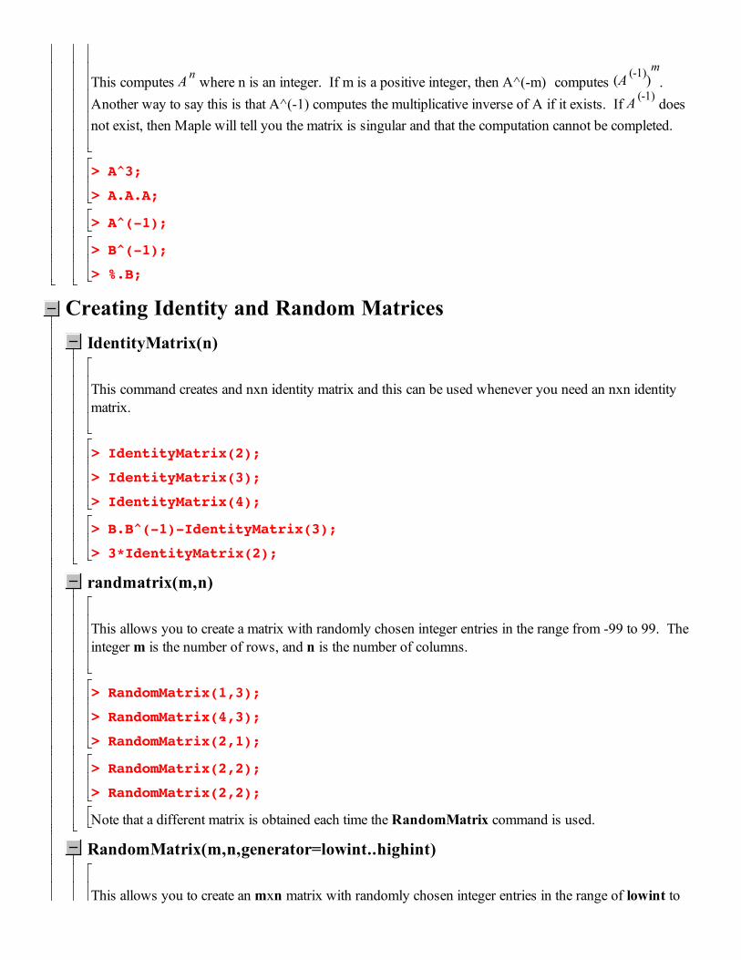
This computes A n where n is an integer. If m is a positive integer, then A^(-m) computes A -1( )( )m
. Another way to say this is that A^(-1) computes the multiplicative inverse of A if it exists. If A -1( ) does not exist, then Maple will tell you the matrix is singular and that the computation cannot be completed.
> A^3;
> A.A.A;
> A^(-1);
> B^(-1);
> %.B;
Creating Identity and Random MatricesIdentityMatrix(n)
This command creates and nxn identity matrix and this can be used whenever you need an nxn identity matrix.
> IdentityMatrix(2);
> IdentityMatrix(3);
> IdentityMatrix(4);
> B.B^(-1)-IdentityMatrix(3);
> 3*IdentityMatrix(2);
randmatrix(m,n)
This allows you to create a matrix with randomly chosen integer entries in the range from -99 to 99. The integer m is the number of rows, and n is the number of columns.
> RandomMatrix(1,3);
> RandomMatrix(4,3);
> RandomMatrix(2,1);
> RandomMatrix(2,2);
> RandomMatrix(2,2);
Note that a different matrix is obtained each time the RandomMatrix command is used.
RandomMatrix(m,n,generator=lowint..highint)
This allows you to create an mxn matrix with randomly chosen integer entries in the range of lowint to

highint. Again m represents the number of rows and n the number of columns.
> M:=RandomMatrix(3,4,generator=-4..7);
The Transpose and Inverse of a MatrixTranspose(A)
Issuing this command results in output which is the transpose of the matrix A.
> A:=RandomMatrix(2,4,generator=-9..9);
> B:=Transpose(A);
> Transpose(B)-A;
MatrixInverse(S)
The command gives as output the inverse of the square matrix S if it exists. Otherwise it tells you the matrix S is singular (noninvertible).
> S:=RandomMatrix(2,2,generator=-5..5);
> T:=MatrixInverse(S);
> S.T;
> T.S;
> M:=<<1,4,7>|<2,5,8>|<3,6,9>>;
> MatrixInverse(M);
Matrix Operations (revisited)
The MatrixInverse and Transpose commands can be used in conjunction with operator symbols.
> MatrixInverse(T)+Transpose(S);
Note that one can verify some identities for nxn matrices where n is fixed. For example, let us verify that A -1( )( )
T = A T( )
-1( ) for an arbitrary 2x2 invertible matrix A.
> A:=<<a,b>|<c,d>>;
> Transpose(MatrixInverse(A));
> MatrixInverse(Transpose(A));

We observe that the above two matrices are equal, and hence the desired identity is established for 2x2 matrices. Of course the equality of the above two matrices could have been more simply observed by noting that the following gives:
> Transpose(A^(-1))-(Transpose(A))^(-1);
Finally, note that this does not prove the identity, in general, for nxn matrices. We could use Maple to verify the identity for 3x3 matrices, then 4x4 matrices, then 5x5 matrices, etc. But we would never finish this program in our lifetime. We must have some other approach to verify the identity in general.
Help
You can get help on most linear algebra commands by simply typing in general, help(LinearAlgebra[command name]). For example:
> help(LinearAlgebra[RandomMatrix]);
>
For help, in general, on the linear algebra package go to Linear Algebra.
Matrix Arithmetic Problems
Turn in a printout of your work (not of the examples). Label problems clearly. Remember to save your work fairly regularly (z S), so that if a system error does occur, most of your work will not be lost. You may want to clear Maple variables after each problem (restart).
Problem 1
Let A =
-7 -8 4
-2 -3 -1
8 -5 5
éêêêêë
ùúúúúû
and B =
3 8 -9
-9 7 -3
-2 5 2
éêêêêë
ùúúúúû
. Compute the following:
a) 2A
b) A+B

c) 3A - 4B
d) 2 A( )T - 3 B( )T
e) AB
f) BA
g) A T B T
h) B A( )T
Problem 2
Let C =
2 4
-5 -5
4 -2
éêêêêë
ùúúúúû
and D = -1 3
1 -4
éêêë
ùúúû
. Verify that:
a) 2(CD)= (2C)D = C(2D)
b) C D( )T = D T C T
Problem 3
Let F = a b
c d
éêêë
ùúúû
, G = e f
g h
éêêë
ùúúû
, and H = i j
k l
éêêë
ùúúû
. Verify that:
a) (F + G) + H = F + (G + H)
b) (FG)H = F(GH)
c) F(G + H) = FG + FH
d) (G + H)F = GF + HF
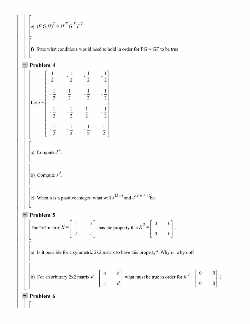
e) F G H( )T = H T G T F T
f) State what conditions would need to hold in order for FG = GF to be true.
Problem 4
Let J =
12
- 12
- 12
- 12
- 12
12
- 12
- 12
- 12
- 12
12
- 12
- 12
- 12
- 12
12
éêêêêêêêêêêêêêêë
ùúúúúúúúúúúúúúúû
.
a) Compute J 2.
b) Compute J 3.
c) When n is a positive integer, what will J 2 n( ) and J 2 n + 1( )be.
Problem 5
The 2x2 matrix K = 1 1
-1 -1
éêêë
ùúúû
has the property that K 2 = 0 0
0 0
éêêë
ùúúû
.
a) Is it possible for a symmetric 2x2 matrix to have this property? Why or why not?
b) For an arbitrary 2x2 matrix K = a b
c d
éêêë
ùúúû
what must be true in order for K 2 = 0 0
0 0
éêêë
ùúúû
?
Problem 6

Find the inverse of each of the following matrices.
a) -1 1
1 0
éêêë
ùúúû
b) 2 6
3 8
éêêë
ùúúû
c)
1 1 1
0 1 1
0 0 1
éêêêêë
ùúúúúû
d)
-1 -3 -3
2 6 1
3 8 3
éêêêêë
ùúúúúû
Problem 7
Let L =
0 2 3 0
0 4 5 0
0 1 0 3
2 0 1 3
éêêêêêêêë
ùúúúúúúúû
a) Find L -1( )
b) Use L -1( ) to solve Lx = b for the following choices of b.
i) b =
1
1
1
1
éêêêêêêêë
ùúúúúúúúû
ii) b =
1
2
3
4
éêêêêêêêë
ùúúúúúúúû

iii) b =
-2
1
0
0
éêêêêêêêë
ùúúúúúúúû
Problem 8
Let M=5 3
3 2
éêêë
ùúúû
, N = 6 2
2 4
éêêë
ùúúû
, and P = 4 -2
-6 3
éêêë
ùúúû
.
Solve each of the following matrix equations for X.
a) MX + N = P
b) XM + N = P