An acceleration of Newton's method:Super-Halley method q

J.M. Guti�errez *, M.A. Hern�andez 1

Universidad de La Rioja, Department of Matem�aticas y Computaci�on, C/ Luis de Ulloa s/n, 26004,

Logro~no, Spain

Abstract

From a study of the convexity we give an acceleration for Newton's method and

obtain a new third order method. Then we use this method for solving non-linear

equations in Banach spaces, establishing conditions on convergence, existence and

uniqueness of solution, as well as error estimates Ó 2001 Elsevier Science Inc. All rights

reserved.

Keywords: Non-linear equation; Newton's method; Kantorovich assumptions; Iterative processes;

Third order method

1. Introduction

The study of concavity and convexity of a real function is an old problemstudied by the mathematicians. It is perfectly established when a function isconcave or convex. However, it is not so developed how to measure thisconcavity or convexity. The degrees of convexity introduced by Jensen andPopoviciu [6] are interesting from the theorical standpoint, but their practicalapplication is too di�cult.

www.elsevier.com/locate/amcApplied Mathematics and Computation 117 (2001) 223±239

q Supported in part by a grant of the DGES PB-96-0120-C03-02 and a grant of the University of

La Rioja API-97/B12.* E-mail address: jmguti@dmc.unirioja.es (J.M. GutieÂrrez).1 E-mail: mahernan@dmc.unirioja.es

0096-3003/01/$ - see front matter Ó 2001 Elsevier Science Inc. All rights reserved.

PII: S0 0 96 -3 0 03 (9 9 )0 01 7 5- 7

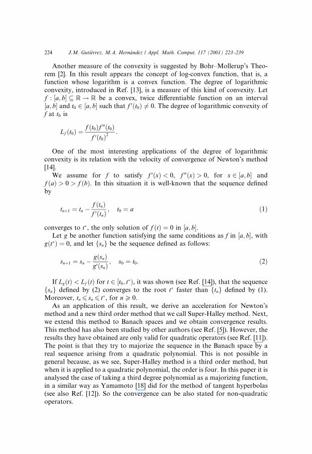
Another measure of the convexity is suggested by Bohr±Mollerup's Theo-rem [2]. In this result appears the concept of log-convex function, that is, afunction whose logarithm is a convex function. The degree of logarithmicconvexity, introduced in Ref. [13], is a measure of this kind of convexity. Letf : �a; b� � R! R be a convex, twice di�erentiable function on an interval�a; b� and t0 2 �a; b� such that f 0�t0� 6� 0. The degree of logarithmic convexity off at t0 is

Lf �t0� � f �t0�f 00�t0�f 0�t0�2

:

One of the most interesting applications of the degree of logarithmicconvexity is its relation with the velocity of convergence of Newton's method[14].

We assume for f to satisfy f 0�x� < 0, f 00�x� > 0, for x 2 �a; b� andf �a� > 0 > f �b�. In this situation it is well-known that the sequence de®nedby

tn�1 � tn ÿ f �tn�f 0�tn� ; t0 � a �1�

converges to t�, the only solution of f �t� � 0 in �a; b�.Let g be another function satisfying the same conditions as f in �a; b�, with

g�t�� � 0, and let fsng be the sequence de®ned as follows:

sn�1 � sn ÿ g�sn�g0�sn� ; s0 � t0: �2�

If Lg�t� < Lf �t� for t 2 �t0; t��, it was shown (see Ref. [14]), that the sequencefsng de®ned by (2) converges to the root t� faster than ftng de®ned by (1).Moreover, tn6 sn6 t�, for n P 0.

As an application of this result, we derive an acceleration for Newton'smethod and a new third order method that we call Super-Halley method. Next,we extend this method to Banach spaces and we obtain convergence results.This method has also been studied by other authors (see Ref. [5]). However, theresults they have obtained are only valid for quadratic operators (see Ref. [11]).The point is that they try to majorize the sequence in the Banach space by areal sequence arising from a quadratic polynomial. This is not possible ingeneral because, as we see, Super-Halley method is a third order method, butwhen it is applied to a quadratic polynomial, the order is four. In this paper it isanalysed the case of taking a third degree polynomial as a majorizing function,in a similar way as Yamamoto [18] did for the method of tangent hyperbolas(see also Ref. [12]). So the convergence can be also stated for non-quadraticoperators.

224 J.M. Guti�errez, M.A. Hern�andez / Appl. Math. Comput. 117 (2001) 223±239

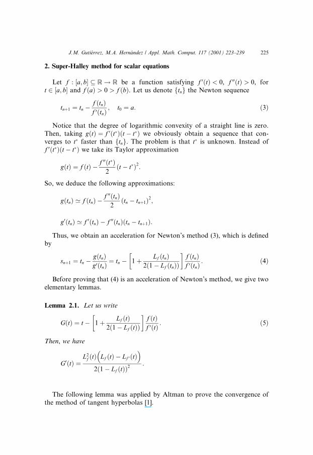
2. Super-Halley method for scalar equations

Let f : �a; b� � R! R be a function satisfying f 0�t� < 0, f 00�t� > 0, fort 2 �a; b� and f �a� > 0 > f �b�. Let us denote ftng the Newton sequence

tn�1 � tn ÿ f �tn�f 0�tn� ; t0 � a: �3�

Notice that the degree of logarithmic convexity of a straight line is zero.Then, taking g�t� � f 0�t���t ÿ t�� we obviously obtain a sequence that con-verges to t� faster than ftng. The problem is that t� is unknown. Instead off 0�t���t ÿ t�� we take its Taylor approximation

g�t� � f �t� ÿ f 00�t��2�t ÿ t��2:

So, we deduce the following approximations:

g�tn� ' f �tn� ÿ f 00�tn�2�tn ÿ tn�1�2;

g0�tn� ' f 0�tn� ÿ f 00�tn��tn ÿ tn�1�:Thus, we obtain an acceleration for Newton's method (3), which is de®ned

by

sn�1 � tn ÿ g�tn�g0�tn� � tn ÿ 1

�� Lf �tn�

2�1ÿ Lf �tn���

f �tn�f 0�tn� : �4�

Before proving that (4) is an acceleration of Newton's method, we give twoelementary lemmas.

Lemma 2.1. Let us write

G�t� � t ÿ 1

�� Lf �t�

2�1ÿ Lf �t���

f �t�f 0�t� : �5�

Then, we have

G0�t� �L2

f �t� Lf �t� ÿ Lf 0 �t�� �

2�1ÿ Lf �t��2:

The following lemma was applied by Altman to prove the convergence ofthe method of tangent hyperbolas [1].

J.M. Guti�errez, M.A. Hern�andez / Appl. Math. Comput. 117 (2001) 223±239 225

Lemma 2.2. Let us assume that f satisfies f �t�P 0 for a6 t6 t�, where t� is aroot of f, i.e., f �t�� � 0: The second derivative f 00 is non-decreasing for a6 t6 t�.Then, Lf �t�6 1=2; for a6 t6 t�:

Theorem 2.3. Under the previous assumptions for f, the sequence fsng defined by(4) is an acceleration of the Newton's method (3).

Proof. Let G the function de®ned by (5), F �t� � t ÿ �f �t�=f 0�t��, ftng and fsnggiven by (3) and (4), respectively. By Lemma 2.1 we have

limn!1

t� ÿ sn�1

t� ÿ tn�1

� limn!1

t� ÿ G�tn�t� ÿ F �tn� � lim

t!t�

t� ÿ G�t�t� ÿ F �t� � 0: �

From this acceleration we can de®ne a new method as follows:

t0 � a; tn�1 � G�tn� � tn ÿ 1

�� Lf �tn�

2�1ÿ Lf �tn���

f �tn�f 0�tn� : �6�

We call (6) Super-Halley method. In the next result we give conditions on theconvergence of (6).

Theorem 2.4. Let us assume that f satisfies f 0�t� < 0, f 00�t� > 0, for t 2 �a; b�,and f �a� > 0 > f �b�. Let t� 2 �a; b� such that f �t�� � 0. Suppose

Lf 0 �t�6 Lf �t� < 1; t 2 �a; t��: �7�Then the sequence ftng defined by (6) converges to t�. In addition, ftng is in-creasing.

Proof. We write (6) in the form tn�1 � 1=2�F �tn� � Q�tn��; where

F �t� � t ÿ f �t�f 0�t� ; Q�t� � t ÿ q�t�

q0�t� ; q�t� � f �t�f 0�t� : �8�

Then, by using the Mean Value Theorem

t� ÿ t1 � F � Q2�t�� ÿ F � Q

2�t0�6 F � Q

2

� �0�z0��t� ÿ t0�

for some z0 2 �t0; t��. Taking into account Lemma 2.1 and (7) we deduce

F 0�t� � Q0�t� � L2f �t�

�1ÿ Lf �t��2Lf �t�h

ÿ Lf 0 �t�iP 0; t 2 �a; t��

and consequently, t16 t�. Following an inductive process is easy to check tn6 t�

for n P 0.

226 J.M. Guti�errez, M.A. Hern�andez / Appl. Math. Comput. 117 (2001) 223±239

On the other hand we have

tn�1 ÿ tn � ÿ f �tn�f 0�tn�H Lf �tn�

ÿ �;

where H�t� � 1� �t=2�1ÿ t��:For n P 0; we derive from Lemma 2.2 thatH�Lf �tn�� > 0 and tn�1 P tn. Then ftng converges to u 2 �a; b�. Making n!1in (6) and taking into account H�Lf �tn��P 1 for n P 0, we have f �u� � 0: As fhas a unique root in �a; b�, we conclude u � t�. �

Note. A su�cient condition for (7) to hold is

f 000�t�P 0; t 2 �t0; t��:In fact, it is known (Lemma 2.2) that f in the previous situation satis®esLf �t� � 1=2 < 1. The ®rst inequality follows inmediately since Lf �t�P0 P Lf 0 �t�, for t 2 �t0; t��:

If (7) is not ful®lled, the convergence of (6) is a hard problem. We cannotguarantee the sequence obtained in this case to be increasing towards t�. In Ref.[13] more general convergence conditions for (6) have been established.

The method (6) is a third order method. This follows as a consequence of theGander's result [8].

Theorem 2.5. Let t� be a simple zero of f and H any function with H�0� � 1,H 0�0� � 1=2, jH 00�0�j <1. The iteration

tn�1 � tn ÿ H Lf �tn�ÿ � f �tn�

f 0�tn�is of third order.

However, if we use the method (6) for solving the equation p�t� � 0, p beinga quadratic polynomial, we obtain a fourth order method, as we state at thenext result.

Theorem 2.6. Let p be a quadratic polynomial with a simple zero t�. The Super-Halley method (6) for solving the equation p�t� � 0 is a fourth order method.

Proof. Let G be the function de®ned by (5). Observe that G�t�� � t�. By Lemma2.1 we obtain, for a quadratic polynomial p,

G0�t� � L3p�t�

2�1ÿ Lp�t��2

and then G0�t�� � 0. We can prove without di�culty that G00�t�� � 0 andG000�t�� � 0 too. However,

J.M. Guti�errez, M.A. Hern�andez / Appl. Math. Comput. 117 (2001) 223±239 227

G�iv��t�� � 3p00�t��3p0�t��3 6� 0: �

The previous results about the order of convergence of the sequence (6) holdif t� is a simple zero of f. When the multiplicity of t� is m > 1, we only canguarantee linear convergence [17].

In Theorem 2.6 we have established that Super-Halley method to solve aequation p�t� � 0, where p is a quadratic polynomial, is a fourth order method.Moreover, we can prove in this case that two iterations of Newton's method isequivalent to one iteration of Super-Halley method.

Theorem 2.7. Let p be a quadratic polynomial with two positive roots. Let ussuppose, without loss of generality, that

p�t� � bt2 ÿ t � a; ab6 1

4:

Denote by fzng the Newton sequence to solve p�t� � 0, and by ftng the iterates(6). Suppose z0 � t0. Then z2n � tn for n P 0:

Proof. Let G and F be the functions de®ned in (5) and (8), respectively. Then,

F F �t�� � � b bt2 ÿ a� �2 ÿ a�2bt ÿ 1�2�2bt ÿ 1� 2b�bt2 ÿ a� ÿ �2bt ÿ 1�� �

� b3t4 ÿ 6ab2t2 � 4abt � a2bÿ a�2bt ÿ 1� 2b�bt2 ÿ a� ÿ �2bt ÿ 1�� � � G�t�:

Therefore, z2 � F �z1� � F F �z0�� � � G�z0� � G�t0� � t1, z4 � F �z3� � F F �z2�� �� G�z2� � G�t1� � t2 and so on. �

3. Super-Halley method in Banach spaces

Let X and Y be Banach spaces and F : X � X ! Y , a non-linear, twiceFr�echet di�erentiable operator in an open convex domain X0 � X. For solvingthe equation

F �x� � 0 �9�we can use the next generalization of (6):

xn�1 � xn ÿ I�� 1

2LF �xn�Dÿ1

n

�CnF �xn�; n P 0; �10�

where x0 2 X0, I is the identity operator on X, Cn � �F 0�xn��ÿ1, Dn � I ÿ LF �xn�� �

and LF �xn� is the following linear operator [10]:

228 J.M. Guti�errez, M.A. Hern�andez / Appl. Math. Comput. 117 (2001) 223±239

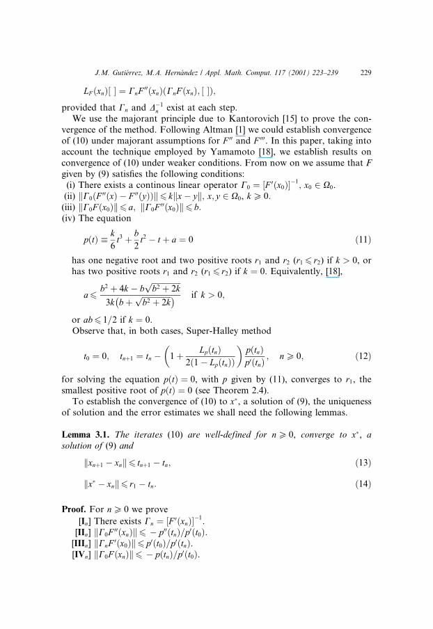
LF �xn�� � � CnF 00�xn� CnF �xn�; � �� �;provided that Cn and Dÿ1

n exist at each step.We use the majorant principle due to Kantorovich [15] to prove the con-

vergence of the method. Following Altman [1] we could establish convergenceof (10) under majorant assumptions for F 00 and F 000. In this paper, taking intoaccount the technique employed by Yamamoto [18], we establish results onconvergence of (10) under weaker conditions. From now on we assume that Fgiven by (9) satis®es the following conditions:

(i) There exists a continous linear operator C0 � �F 0�x0��ÿ1; x0 2 X0.

(ii) kC0�F 00�x� ÿ F 00�y��k6 kkxÿ yk; x; y 2 X0, k P 0:(iii) kC0F �x0�k6 a; kC0F 00�x0�k6 b:(iv) The equation

p�t� � k6

t3 � b2

t2 ÿ t � a � 0 �11�

has one negative root and two positive roots r1 and r2 (r16 r2) if k > 0, orhas two positive roots r1 and r2 (r16 r2) if k � 0. Equivalently, [18],

a6 b2 � 4k ÿ b���������������b2 � 2kp

3k b� ���������������b2 � 2kpÿ � if k > 0;

or ab6 1=2 if k � 0.Observe that, in both cases, Super-Halley method

t0 � 0; tn�1 � tn ÿ 1

�� Lp�tn�

2�1ÿ Lp�tn���

p�tn�p0�tn� ; n P 0; �12�

for solving the equation p�t� � 0, with p given by (11), converges to r1, thesmallest positive root of p�t� � 0 (see Theorem 2.4).

To establish the convergence of (10) to x�, a solution of (9), the uniquenessof solution and the error estimates we shall need the following lemmas.

Lemma 3.1. The iterates (10) are well-defined for n P 0, converge to x�, asolution of (9) and

kxn�1 ÿ xnk6 tn�1 ÿ tn; �13�

kx� ÿ xnk6 r1 ÿ tn: �14�

Proof. For n P 0 we prove

[In] There exists Cn � �F 0�xn��ÿ1.

[IIn] kC0F 00�xn�k6 ÿ p00�tn�=p0�t0�:[IIIn] kCnF 0�x0�k6 p0�t0�=p0�tn�.[IVn] kC0F �xn�k6 ÿ p�tn�=p0�t0�.

J.M. Guti�errez, M.A. Hern�andez / Appl. Math. Comput. 117 (2001) 223±239 229

[Vn] There exists Dÿ1n � �I ÿ LF �xn��ÿ1

and kDÿ1n k6 1=�1ÿ Lp�tn��.

Note that [Vn�1] follows as a consequence of [IIn�1], [IIIn�1], [IVn�1] andLemma 2.2 which guarantees Lp�t�6 1=2. Thus, we prove [In�1]±[IVn�1] usinginduction. Applying Altman's technique, (see Ref. [1]), [In�1], [IIn�1] and [IIIn�1]follow inmediately.

To prove [IVn�1], using Taylor's formula and (10), we obtain

F �xn�1� � ÿ 1

2F 00�xn�CnF �xn�Dÿ1

n CnF �xn� � 1

2F 00�xn��xn�1 ÿ xn�2

�Z xn�1

xn

F 00�x�� ÿ F 00�xn���xn�1 ÿ x�dx

� ÿ 1

2F 00�xn�CnF �xn�Dÿ1

n CnF �xn�

� 1

2F 00�xn� CnF �xn�� �2 � 1

8F 00�xn� LF �xn�Dÿ1

n CnF �xn�� �2

� 1

2F 00�xn�CnF �xn�LF �xn�Dÿ1

n CnF �xn�

�Z xn�1

xn

�F 00�x� ÿ F 00�xn���xn�1 ÿ x�dx:

Bearing in mind Dÿ1n � I � LF �xn�Dÿ1

n and writing yn � LF �xn�Dÿ1n CnF �xn�, we

have

F �xn�1� � 1

8F 00�xn�y2

n �Z xn�1

xn

�F 00�x� ÿ F 00�xn���xn�1 ÿ x�dx:

Denote sn � Lp�tn�. Notice that

kynk6 kLF �xn�kkDÿ1n kkCnF �xn�k6 ÿ snp�tn�

�1ÿ sn�p0�tn�and therefore,

kC0F �xn�1�k6 1

8

s3np�tn��1ÿ sn�2

� k6kxn�1 ÿ xnk36 1

8

s3np�tn��1ÿ sn�2

� k6�tn�1 ÿ tn�3:

Consequently

kC0F �xn�1�k6 p�tn�1� �15�and we conclude the induction.

So, we have

kxn�1 ÿ xnk � I� � 1

2LF �xn�

�Dÿ1

n CnF �xn�

6 1

�� Lp�tn�

2�1ÿ Lp�tn���

p�tn�p0�tn� � tn�1 ÿ tn;

230 J.M. Guti�errez, M.A. Hern�andez / Appl. Math. Comput. 117 (2001) 223±239

then (13) happens and ftng majorizes fxng. The convergence of ftng (see The-orem 2.4 and its note) implies the convergence of fxng to a limit x�. Makingn!1 in (15), we deduce F �x�� � 0.

Finally, for p P 0, kxn�p ÿ xnk6 tn�p ÿ tn: Making p !1 we obtain (14).�

Lemma 3.2. Under the previous assumptions we have, for k > 0,

kx� ÿ xn�1kr1 ÿ tn�1

6 kx� ÿ xnkr1 ÿ tn

� �3

; n P 0

and, for k � 0,

kx� ÿ xn�1kr1 ÿ tn�1

6 kx� ÿ xnkr1 ÿ tn

� �4

; n P 0:

Proof. This proof follows the technique used by Yamamoto in Ref. [18] for themethod of tangent hyperbolas. Observe that Dÿ1

n � I � LF �xn�Dÿ1n and then,

I � 1

2LF �xn�Dÿ1

n �1

2�I � Dÿ1

n � �1

2Dÿ1

n �Dn � I� � Dÿ1n I�ÿ 1

2LF �xn�

�:

Taking this into account we deduce

x� ÿ xn�1 � x� ÿ xn �Dÿ1n I�ÿ 1

2LF �xn�

�CnF �xn�

� ÿ Dÿ1n Cn F �x��

�ÿ F �xn� ÿ F 0�xn��x� ÿ xn� ÿ 1

2F 00�xn��x� ÿ xn�2

�� �x� ÿ xn� ÿ 1

2Dÿ1

n LF �xn�CnF �xn� ÿ Dÿ1n �x� ÿ xn�

ÿ 1

2Dÿ1

n CnF 00�xn��x� ÿ xn�2

� ÿ Dÿ1n Cn

Z x�

xn

F 00�x�� ÿ F 00�xn���x� ÿ x�dx� I

� ÿ Dÿ1n

��x� ÿ xn�

ÿ 1

2Dÿ1

n CnF 00�xn� �CnF �xn���2h

� �x� ÿ xn�2i

� ÿ Dÿ1n Cn

Z x�

xn

F 00�x�� ÿ F 00�xn���x� ÿ x�dx

ÿ 1

2Dÿ1

n CnF 00�xn� Cn

Z x�

xn

F 00�x��x��

ÿ x�dx�2

and therefore

J.M. Guti�errez, M.A. Hern�andez / Appl. Math. Comput. 117 (2001) 223±239 231

kx� ÿ xn�1k6 kDÿ1n kkCnF 0�x0�k

Z x�

xn

C0�F 00�x� ÿ F 00�xn���x� ÿ x�dx

� 1

2kDÿ1

n kkCnF 0�x0�kkC0F 00�xn�k Cn

Z x�

xn

F 00�x��x� ÿ x�dx

2

6 ÿ k�r1 ÿ tn�36p0�tn��1ÿ Lp�tn��

kx� ÿ xnkr1 ÿ tn

� �3

ÿ p00�tn�2p0�tn�3�1ÿ Lp�tn��

Z r1

tn

p00�z��r1

�ÿ z�dz

�2 kx� ÿ xnkr1 ÿ tn

� �4

: �16�

For k > 0, from (14), we have

kx� ÿ xn�1k6 ÿ k�r1 ÿ tn�36p0�tn��1ÿ Lp�tn��

"� p00�tn�

2p0�tn�3�1ÿ Lp�tn��

�Z r1

tn

p00�z��r1

�ÿ z�dz

�2#kx� ÿ xnk

r1 ÿ tn

� �3

� �r1 ÿ tn�1� kx� ÿ xnk

r1 ÿ tn

� �3

:

But if k � 0, from (16), we deduce

kx� ÿ xn�1k6 ÿ p00�tn�2p0�tn�3�1ÿ Lp�tn��

Z r1

tn

p00�z��r1

�ÿ z�dz

�2 kx� ÿ xnkr1 ÿ tn

� �4

� �r1 ÿ tn�1� kx� ÿ xnk

r1 ÿ tn

� �4

: �

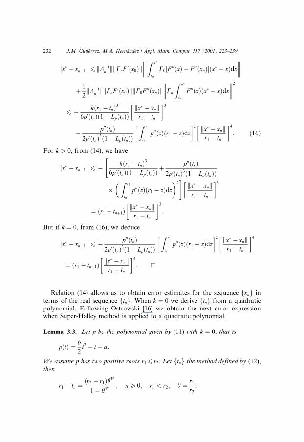
Relation (14) allows us to obtain error estimates for the sequence fxng interms of the real sequence ftng. When k � 0 we derive ftng from a quadraticpolynomial. Following Ostrowski [16] we obtain the next error expressionwhen Super-Halley method is applied to a quadratic polynomial.

Lemma 3.3. Let p be the polynomial given by (11) with k � 0, that is

p�t� � b2

t2 ÿ t � a:

We assume p has two positive roots r16 r2. Let ftng the method defined by (12),then

r1 ÿ tn � �r2 ÿ r1�h4n

1ÿ h4n ; n P 0; r1 < r2; h � r1

r2

;

232 J.M. Guti�errez, M.A. Hern�andez / Appl. Math. Comput. 117 (2001) 223±239

r1 ÿ tn � r1

4n; n P 0; r1 � r2:

When k > 0 the real sequence ftng in (14) is obtained from a cubic poly-nomial. In this case, it is di�cult to obtain an error expression by Ostrowskimethod. In the next lemma and in a di�erent way [12], we establish estimatesfor the error in this situation.

Lemma 3.4. Let p be the polynomial given by (11) with k > 0, that is

p�t� � k6

t3 � b2

t2 ÿ t � a:

Let us assume that p has two positive roots r16 r2 and a negative root, ÿr0. Let usconsider Super-Halley method ftng defined by (12), then, if r1 < r2;

r1 ÿ tn � �r2 ÿ r1�h3n���kp ÿ h3n ; n P 0;

where

k � r2 ÿ r1

r0 � r1

< 1; h ����kp r1

r2

< 1:

If r1 � r2, we haver1

4n6 r1 ÿ tn6

r1

3n:

Proof. The polynomial p de®ned above can be written in the form

p�t� � k6�r1 ÿ t��r2 ÿ t��r0 � t�:

Notice that comparing the coe�cients of t2 we obtain r1 � r26 r0.Let us write an � r1 ÿ tn, bn � r2 ÿ tn and cn � r0 � tn. Then p�tn� � 1

6kanbncn,

p0�tn� � 16k�anbn ÿ ancn ÿ bncn� and p00�tn� � 1

6k�2cn ÿ 2an ÿ 2bn�. Thus, taking

into account (12), we have

an�1 � r1 ÿ tn�1 � r1 ÿ tn � 1

�� Lp�tn�

2�1ÿ Lp�tn���

p�tn�p0�tn�

� k6

� �3 a3n

p0�tn�3�1ÿ Lp�tn��an�bn

� ÿ cn��b2n � c2

n� ÿ b2nc2

n

�:

In a similar way, we deduce

bn�1 � k6

� �3 b3n

p0�tn�3�1ÿ Lp�tn��bn�an

� ÿ cn��a2n � c2

n� ÿ a2nc2

n

�:

J.M. Guti�errez, M.A. Hern�andez / Appl. Math. Comput. 117 (2001) 223±239 233

Consequently,

an�1

bn�1

� a3n

b3n

H�tn�;

where

H�tn� � b2nc2

n � an�cn ÿ bn��b2n � c2

n�a2

nc2n � bn�cn ÿ an��a2

n � c2n�:

Notice that

H�tn� � b3nan�1

a3nbn�1

� �r1 ÿ G�tn���r2 ÿ tn�3�r2 ÿ G�tn���r1 ÿ tn�3

;

with G de®ned in (5). As G�r1� � r1, G0�r1� � G00�r1� � 0, we have for t close tor1

H�t� � G000�r1�6�r2 ÿ r1�2 � ÿ f 000�r1�

6f 0�r1� �r2 ÿ r1�2 � r2 ÿ r1

r0 � r1

:

Since tn ! r1 when n!1, we obtain

an

bn� anÿ1

bnÿ1

� �3

k � � � � � a0

b0

� �3n

k�3nÿ1�=2 �

���kp r1

r2

� �3n

1���kp :

Then, r1 ÿ tn � �r2 ÿ r1 � r1 ÿ tn��h3n=���kp � and the ®rst part follows.

If r1 � r2, we can write p�t� � 16k�r1 ÿ t�2�r0 � t�, where 2r16 r0. With the

same technique and notations, we obtain

an�1 � ana3

n ÿ cna2n ÿ c3

n

�an ÿ 2cn��a2n � 2c2

n�� an

an=cn� �3 ÿ an=cn� �2 ÿ 1

�an=cn� ÿ 2� � an=cn� �2 � 2� � :

Taking into account that an=cn6 12

and the function

f �x� � 1� x2 ÿ x3

�x2 � 2��2ÿ x�

increases in �0; 1=2�, we deduce an=46 an�16 an=3 and the result follows. �

Theorem 3.5. Let us assume (i)±(iv) and in addition

B � B�x1; r1 ÿ t1� � fx 2 X ; kxÿ x1k6 r1 ÿ t1g � X0:

Then the iterative method defined by (10) is well-defined, xn 2 B (interior of B) forn P 1 and the sequence fxng is convergent to x�, solution of (9). If r1 < r2 we have

234 J.M. Guti�errez, M.A. Hern�andez / Appl. Math. Comput. 117 (2001) 223±239

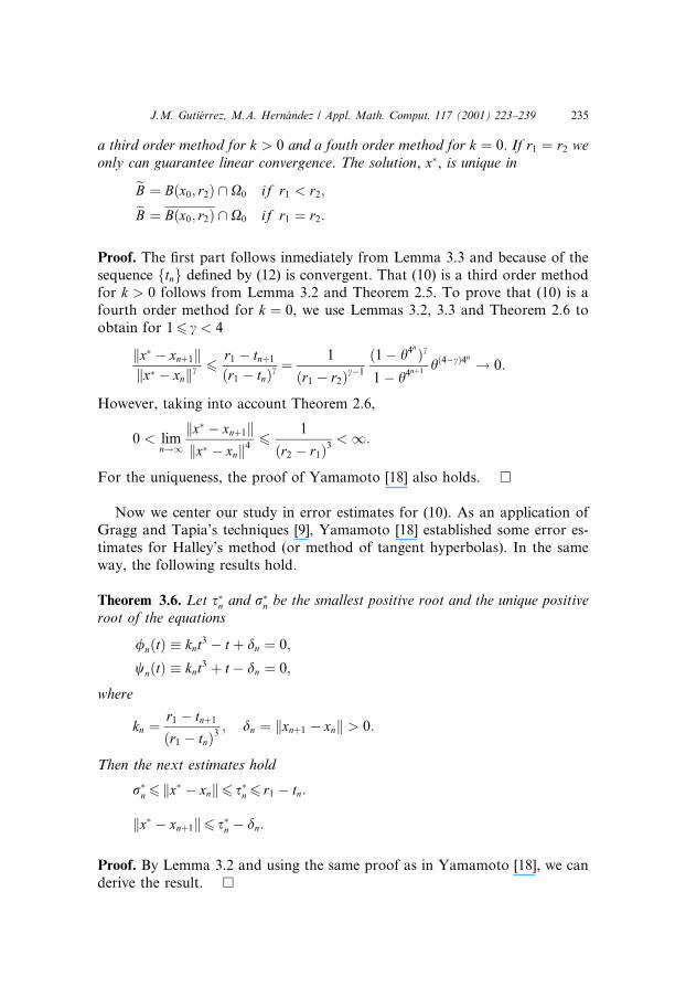
a third order method for k > 0 and a fouth order method for k � 0. If r1 � r2 weonly can guarantee linear convergence. The solution, x�, is unique ineB � B�x0; r2� \ X0 if r1 < r2;eB � B�x0; r2� \ X0 if r1 � r2:

Proof. The ®rst part follows inmediately from Lemma 3.3 and because of thesequence ftng de®ned by (12) is convergent. That (10) is a third order methodfor k > 0 follows from Lemma 3.2 and Theorem 2.5. To prove that (10) is afourth order method for k � 0, we use Lemmas 3.2, 3.3 and Theorem 2.6 toobtain for 16 c < 4

kx� ÿ xn�1kkx� ÿ xnkc 6

r1 ÿ tn�1

�r1 ÿ tn�c �1

�r1 ÿ r2�cÿ1

�1ÿ h4n�c1ÿ h4n�1 h�4ÿc�4n ! 0:

However, taking into account Theorem 2.6,

0 < limn!1kx� ÿ xn�1kkx� ÿ xnk4

6 1

�r2 ÿ r1�3<1:

For the uniqueness, the proof of Yamamoto [18] also holds. �

Now we center our study in error estimates for (10). As an application ofGragg and Tapia's techniques [9], Yamamoto [18] established some error es-timates for Halley's method (or method of tangent hyperbolas). In the sameway, the following results hold.

Theorem 3.6. Let s�n and r�n be the smallest positive root and the unique positiveroot of the equations

/n�t� � knt3 ÿ t � dn � 0;

wn�t� � knt3 � t ÿ dn � 0;

where

kn � r1 ÿ tn�1

�r1 ÿ tn�3; dn � kxn�1 ÿ xnk > 0:

Then the next estimates hold

r�n6 kx� ÿ xnk6 s�n6 r1 ÿ tn:

kx� ÿ xn�1k6 s�n ÿ dn:

Proof. By Lemma 3.2 and using the same proof as in Yamamoto [18], we canderive the result. �

J.M. Guti�errez, M.A. Hern�andez / Appl. Math. Comput. 117 (2001) 223±239 235

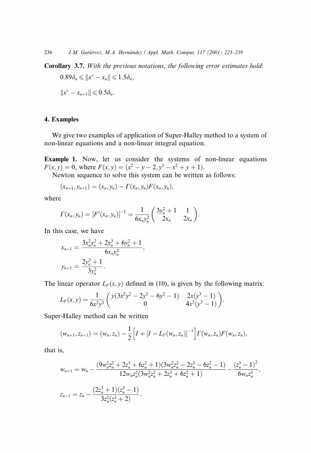
Corollary 3.7. With the previous notations, the following error estimates hold:

0:89dn6 kx� ÿ xnk6 1:5dn;

kx� ÿ xn�1k6 0:5dn:

4. Examples

We give two examples of application of Super-Halley method to a system ofnon-linear equations and a non-linear integral equation.

Example 1. Now, let us consider the systems of non-linear equationsF �x; y� � 0, where F �x; y� � �x2 ÿ y ÿ 2; y3 ÿ x2 � y � 1�.

Newton sequence to solve this system can be written as follows:

�xn�1; yn�1� � �xn; yn� ÿ C�xn; yn�F �xn; yn�;where

C�xn; yn� � �F 0�xn; yn��ÿ1 � 1

6xny2n

3y2n � 1 12xn 2xn

� �:

In this case, we have

xn�1 � 3x2ny2

n � 2y3n � 6y2

n � 1

6xny2n

;

yn�1 � 2y3n � 1

3y2n

:

The linear operator LF �x; y� de®ned in (10), is given by the following matrix:

LF �x; y� � 1

6x2y3

y�3x2y2 ÿ 2y3 ÿ 6y2 ÿ 1� 2x�y3 ÿ 1�0 4x2�y3 ÿ 1�

� �:

Super-Halley method can be written

�wn�1; zn�1� � �wn; zn� ÿ 1

2Ih� �I ÿ LF �wn; zn��ÿ1

iC�wn; zn�F �wn; zn�;

that is,

wn�1 � wn ÿ �9w2nz2

n � 2z3n � 6z2

n � 1��3w2nz2

n ÿ 2z3n ÿ 6z2

n ÿ 1�12wnz2

n�3w2nz2

n � 2z3n � 6z2

n � 1� ÿ �z3n ÿ 1�26wnz5

n

;

zn�1 � zn ÿ �2z3n � 1��z3

n ÿ 1�3z2

n�z3n � 2� :

236 J.M. Guti�errez, M.A. Hern�andez / Appl. Math. Comput. 117 (2001) 223±239

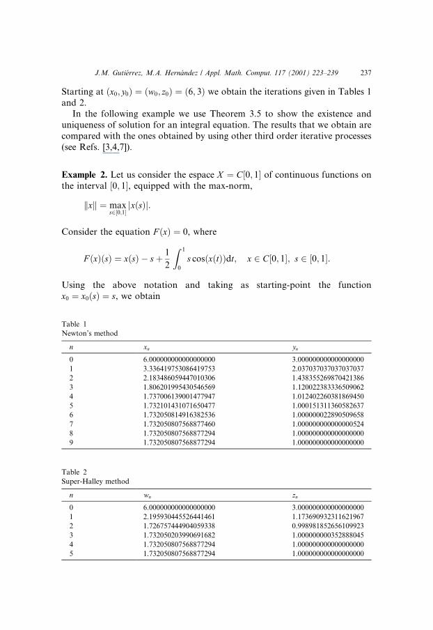
Starting at �x0; y0� � �w0; z0� � �6; 3� we obtain the iterations given in Tables 1and 2.

In the following example we use Theorem 3.5 to show the existence anduniqueness of solution for an integral equation. The results that we obtain arecompared with the ones obtained by using other third order iterative processes(see Refs. [3,4,7]).

Example 2. Let us consider the espace X � C�0; 1� of continuous functions onthe interval �0; 1�, equipped with the max-norm,

kxk � maxs2�0;1�

x�s�j j:

Consider the equation F �x� � 0, where

F �x��s� � x�s� ÿ s� 1

2

Z 1

0

s cos�x�t��dt; x 2 C�0; 1�; s 2 �0; 1�:

Using the above notation and taking as starting-point the functionx0 � x0�s� � s, we obtain

Table 1

Newton's method

n xn yn

0 6.000000000000000000 3.000000000000000000

1 3.336419753086419753 2.037037037037037037

2 2.183486059447010306 1.438355269870421386

3 1.806201995430546569 1.120022383336509062

4 1.737006139001477947 1.012402260381869450

5 1.732101431071650477 1.000151311360582637

6 1.732050814916382536 1.000000022890509658

7 1.732050807568877460 1.000000000000000524

8 1.732050807568877294 1.000000000000000000

9 1.732050807568877294 1.000000000000000000

Table 2

Super-Halley method

n wn zn

0 6.000000000000000000 3.000000000000000000

1 2.195930445526441461 1.173690932311621967

2 1.726757444904059338 0.998981852656109923

3 1.732050203990691682 1.000000000352888045

4 1.732050807568877294 1.000000000000000000

5 1.732050807568877294 1.000000000000000000

J.M. Guti�errez, M.A. Hern�andez / Appl. Math. Comput. 117 (2001) 223±239 237

F 0�z�x�s� � x�s� ÿ s2

Z 1

0

x�t� sin�z�t��dt;

�F 0�z��ÿ1y�s� � y�s� � s2Uz

Z 1

0

y�t� sin�z�t��dt;

where

Uz � 1ÿ 1

2

Z 1

0

t sin�z�t��dt;

F 00�z�xy�s� � ÿ s2

Z 1

0

x�t�y�t� cos�z�t��dt;

for x; y; z 2 C�0; 1� and s 2 �0; 1�: So we deduce

a � b � sin 1

2ÿ sin 1� cos 1; k � 1

2ÿ sin 1� cos 1:

In this case the majorizing polynomial is

p�t� � k6

t3 ÿ b2

t2 ÿ t � a

� 1

6�2ÿ sin 1� cos 1� t3� � 3�sin 1�t2 ÿ 6�2ÿ sin 1� cos 1�t � 6 sin 1

�which has two positive roots

r1 � 0:6095694860276291; r2 � 1:70990829134757:

Consequently, Theorem 3.5 guarantees that F �x� � 0 has a root in B�x0; r1� andthis is the only root in B�x0; r2� (we have written B�x0; r� � fx 2 X ; kxÿ x0k6 rgand B�x0; r� the corresponding closed ball).

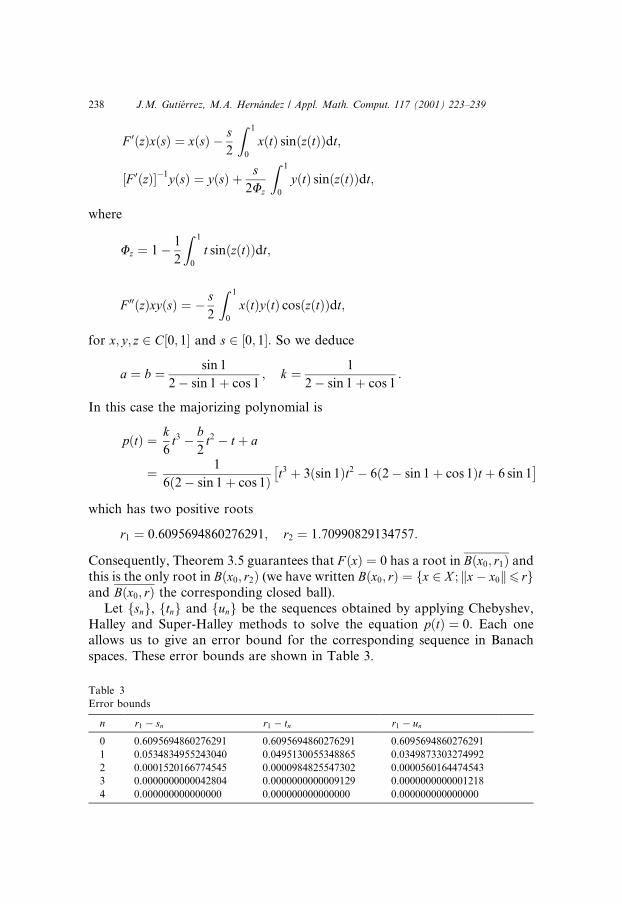
Let fsng, ftng and fung be the sequences obtained by applying Chebyshev,Halley and Super-Halley methods to solve the equation p�t� � 0. Each oneallows us to give an error bound for the corresponding sequence in Banachspaces. These error bounds are shown in Table 3.

Table 3

Error bounds

n r1 ÿ sn r1 ÿ tn r1 ÿ un

0 0.6095694860276291 0.6095694860276291 0.6095694860276291

1 0.0534834955243040 0.0495130055348865 0.0349873303274992

2 0.0001520166774545 0.0000984825547302 0.0000560164474543

3 0.0000000000042804 0.0000000000009129 0.0000000000001218

4 0.000000000000000 0.000000000000000 0.000000000000000

238 J.M. Guti�errez, M.A. Hern�andez / Appl. Math. Comput. 117 (2001) 223±239

Notice that the best error bounds are attained with Super-Halley method.For this equation and using Halley method, D�oring [7] gave the bound

kx� ÿ x2k6 0:000825:

Later, Candela and Marquina [3,4], gave the bounds

kx� ÿ x2k6 0:00037022683427694

and

kx� ÿ x2k6 0:00014987029635502

with Chebyshev and Halley method, respectively.

References

[1] M. Altman, Concerning the method of tangent hyperbolas for operator equations, Bull. Acad.

Pol. Sci., Serie Sci. Math., Ast. et Phys. 9 (1961) 633±637.

[2] R. Campbell, Les Integrales Euleriennes et Leurs Aplications, Dunod, Paris, 1966.

[3] V. Candela, A. Marquina, Recurrence relations for rational cubic methods I: The Halley

method, Comput. 44 (1990) 169±184.

[4] V. Candela, A. Marquina, Recurrence relations for rational cubic methods II: The Chebyshev

method, Comput. 45 (1990) 355±367.

[5] D. Chen, I.K. Argyros, Q.S. Qian, A local convergence theorem for the Super-Halley method

in a Banach space, App. Math. Lett. 7 (5) (1994) 49±52.

[6] Z. Ciesielski, Some propierties of convex functions of higher orders, Annales Polonici

Mathematici 7 (1959) 1±7.

[7] B. D�oring, Einige s�atze �uber das verfahren der tangierenden hyperbeln in Banach-R�aumen,

Aplikace Mat. 15 (1970) 418±464.

[8] W. Gander, On Halley's iteration method, Amer. Math. Monthly 92 (1985) 131±134.

[9] W.B. Gragg, R.A. Tapia, Optimal error bounds for the Newton±Kantorovich theorem, SIAM

J. Numer. Anal. 11 (1974) 10±13.

[10] J.M. Guti�errez, M.A. Hern�andez, M.A. Salanova, Accesibility of solutions by Newton's

method, Int. J. Comput. Math. 57 (1995) 239±247.

[11] J.M. Guti�errez, M.A. Hern�andez, M.A. Salanova, Resolution of quadratic equations in

Banach spaces, Numer. Funct. Anal. Opt. 17 (1/2) (1996) 113±121.

[12] J.M. Guti�errez, M.A. Hern�andez, A family of Chebyshev±Halley type methods in Banach

spaces, Bull. Austral. Math. Soc. 55 (1997) 113±130.

[13] M.A. Hern�andez, Newton±Raphson's method and convexity, Zb. Rad. Prirod.-Mat. Fak. Ser.

Mat. 22 (1) (1993) 159±166.

[14] M.A. Hern�andez, M.A. Salanova, A family of Newton type iterative processes, Int. J. Comput.

Math. 51 (1994) 205±214.

[15] L.V. Kantorovich, G.P. Akilov, Functional Analysis, Pergamon Press, Oxford, 1982.

[16] A.M. Ostrowski, Solution of Equations in Euclidean and Banach Spaces, Academic Press,

New York, 1943.

[17] J.F. Traub, Iterative Methods for Solution of Equations, Prentice-Hall, Englewood Cli�s, NJ,

1964.

[18] T. Yamamoto, On the method of tangent hyperbolas in Banach spaces, J. Comput. Appl.

Math. 21 (1988) 75±86.

J.M. Guti�errez, M.A. Hern�andez / Appl. Math. Comput. 117 (2001) 223±239 239