Simplex method - SRCC
20
Simplex method Simplex method is the method to solve ( LPP ) models which contain two or more decision variables. Basic variables: Are the variables which coefficients One in the equations and Zero in the other equations. Non-Basic variables: Are the variables which coefficients are taking any of the values, whether positive or negative or zero. Slack, surplus & artificial variables: a) If the inequality be (less than or equal, then we add a slack variable + S to change to =. b) If the inequality be (greater than or equal, then we subtract a surplus variable - S to change to =. c) If we have = we use artificial variables. The steps of the simplex method: Step 1: Determine a starting basic feasible solution. Step 2: Select an entering variable using the optimality condition. Stop if there is no entering variable. Step 3: Select a leaving variable using the feasibility condition.
-
Upload
khangminh22 -
Category
Documents
-
view
5 -
download
0
Transcript of Simplex method - SRCC

Simplex method
Simplex method is the method to solve ( LPP ) models which contain two or
more decision variables.
Basic variables:
Are the variables which coefficients One in the equations and Zero in the
other equations.
Non-Basic variables:
Are the variables which coefficients are taking any of the values, whether
positive or negative or zero.
Slack, surplus & artificial variables:
a) If the inequality be (less than or equal, then we add a slack
variable + S to change to =.
b) If the inequality be (greater than or equal, then we
subtract a surplus variable - S to change to =.
c) If we have = we use artificial variables.
The steps of the simplex method:
Step 1:
Determine a starting basic feasible solution.
Step 2:
Select an entering variable using the optimality condition. Stop if
there is no entering variable.
Step 3:
Select a leaving variable using the feasibility condition.
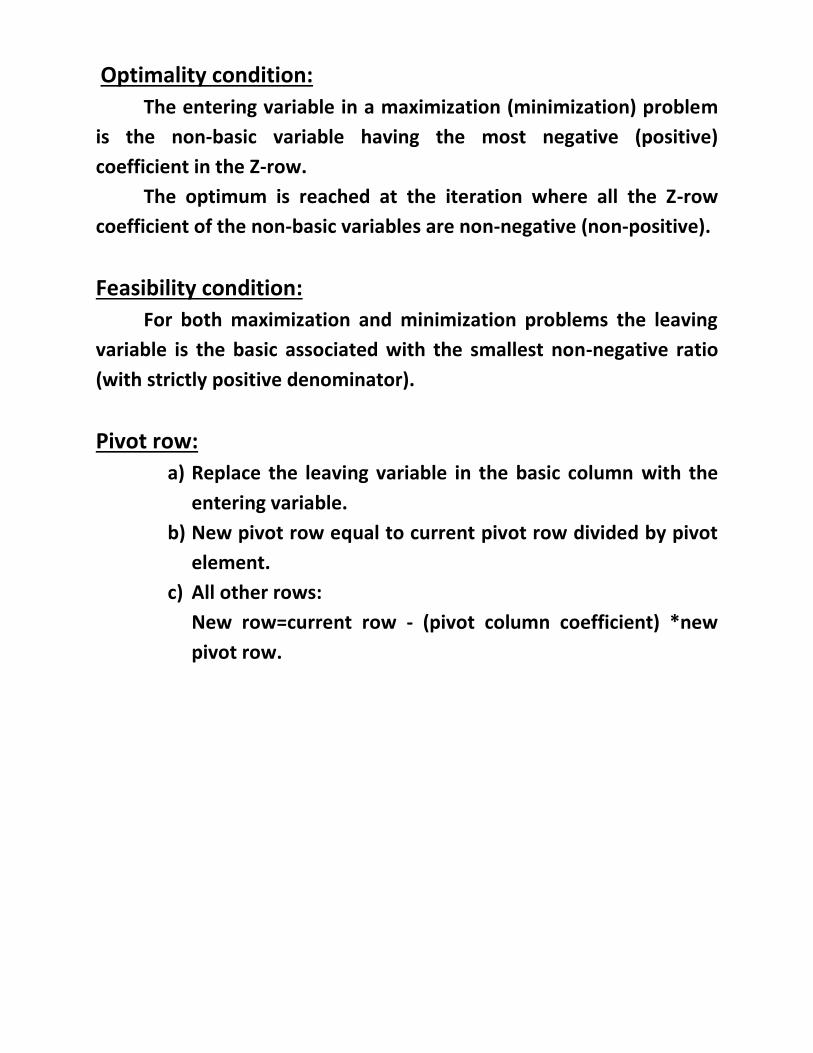
Optimality condition:
The entering variable in a maximization (minimization) problem
is the non-basic variable having the most negative (positive)
coefficient in the Z-row.
The optimum is reached at the iteration where all the Z-row
coefficient of the non-basic variables are non-negative (non-positive).
Feasibility condition:
For both maximization and minimization problems the leaving
variable is the basic associated with the smallest non-negative ratio
(with strictly positive denominator).
Pivot row:
a) Replace the leaving variable in the basic column with the
entering variable.
b) New pivot row equal to current pivot row divided by pivot
element.
c) All other rows:
New row=current row - (pivot column coefficient) *new
pivot row.

Example 1:
Use the simplex method to solve the (LP) model:
Subject to
Solution:
Subject to
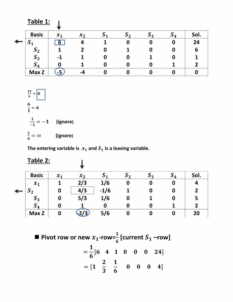
Table 1:
Basic Sol.
6 4 1 0 0 0 24 1 2 0 1 0 0 6 -1 1 0 0 1 0 1 0 1 0 0 0 1 2
Max Z -5 -4 0 0 0 0 0
(ignore)
(ignore)
The entering variable is and is a leaving variable.
Table 2:
Pivot row or new -row=
[current –row]
Basic Sol.
1 2/3 1/6 0 0 0 4
0 4/3 -1/6 1 0 0 2
0 5/3 1/6 0 1 0 5 0 1 0 0 0 1 2
Max Z 0 -2/3 5/6 0 0 0 20
- New -row=[ current –row]-(1)[ new –row]
=[1 2 0 1 0 0 6]- (1)[1 2/3 1/6 0 0 0 0 4]
=[0 4/3 -1/6 1 0 0 2]
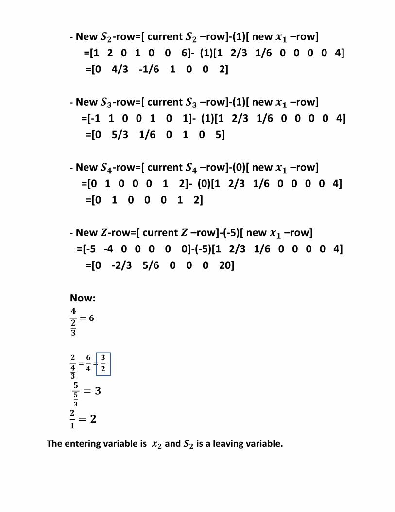
- New -row=[ current –row]-(1)[ new –row]
=[-1 1 0 0 1 0 1]- (1)[1 2/3 1/6 0 0 0 0 4]
=[0 5/3 1/6 0 1 0 5]
- New -row=[ current –row]-(0)[ new –row]
=[0 1 0 0 0 1 2]- (0)[1 2/3 1/6 0 0 0 0 4]
=[0 1 0 0 0 1 2]
- New -row=[ current –row]-(-5)[ new –row]
=[-5 -4 0 0 0 0 0]-(-5)[1 2/3 1/6 0 0 0 0 4]
=[0 -2/3 5/6 0 0 0 20]
Now:
The entering variable is and is a leaving variable.
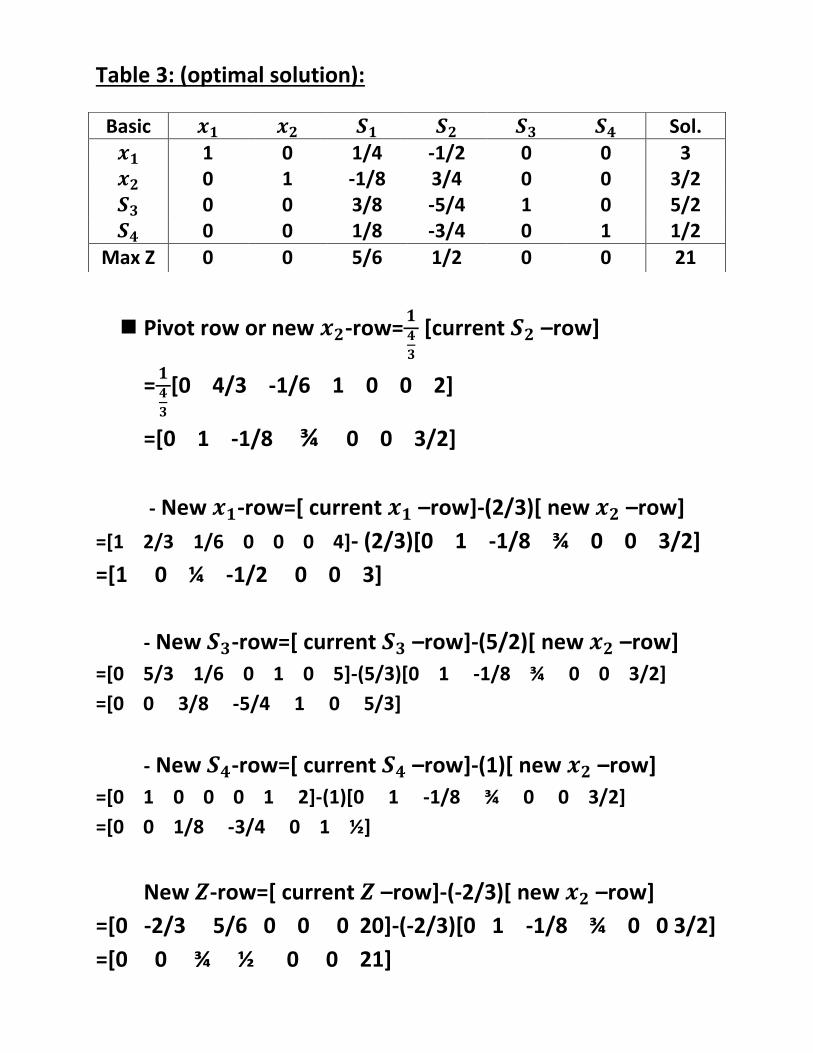
Table 3: (optimal solution):
Pivot row or new -row=
[current –row]
=
[0 4/3 -1/6 1 0 0 2]
=[0 1 -1/8 ¾ 0 0 3/2]
- New -row=[ current –row]-(2/3)[ new –row]
=[1 2/3 1/6 0 0 0 4]- (2/3)[0 1 -1/8 ¾ 0 0 3/2]
=[1 0 ¼ -1/2 0 0 3]
- New -row=[ current –row]-(5/2)[ new –row]
=[0 5/3 1/6 0 1 0 5]-(5/3)[0 1 -1/8 ¾ 0 0 3/2]
=[0 0 3/8 -5/4 1 0 5/3]
- New -row=[ current –row]-(1)[ new –row]
=[0 1 0 0 0 1 2]-(1)[0 1 -1/8 ¾ 0 0 3/2]
=[0 0 1/8 -3/4 0 1 ½]
New -row=[ current –row]-(-2/3)[ new –row]
=[0 -2/3 5/6 0 0 0 20]-(-2/3)[0 1 -1/8 ¾ 0 0 3/2]
=[0 0 ¾ ½ 0 0 21]
Basic Sol.
1 0 1/4 -1/2 0 0 3 0 1 -1/8 3/4 0 0 3/2 0 0 3/8 -5/4 1 0 5/2 0 0 1/8 -3/4 0 1 1/2
Max Z 0 0 5/6 1/2 0 0 21

Then the solution is:
Example 2:
Use the simplex method to solve the (LP) model:
Subject to
Solution:
Subject to
Table 1:
Basic Sol.
0.25 0.5 1 0 0 40 0.4 0.2 0 1 0 40 0 0.8 0 0 1 40
Max Z -2 -3 0 0 0 0

Pivot row or new -row=
[0 0.8 0 0 1 40]
=[0 1 0 0 1.25 50]
New -row=[ current –row]-(0.5)[ new –row]
=[0.25 0.5 1 0 0 40]-(0.5)[0 1 0 0 1.25 50]
=[0 0.5 0 0 -0.625 15]
New -row=[ current –row]-(0.2)[ new –row]
=[0.4 0.2 0 1 0 40]-(0.2)[0 1 0 0 1.25 50]
[0.4 0 0 1 -0.25 30]
New -row=[ current –row]-(-3)[ new –row]
=[-2 -3 0 0 0 0]-(-3)[0 1 0 0 1.25 50]
=[-2 0 0 0 3.75 150]
Table 2:
Basic Sol.
0.25 0 1 0 -0.625 15 0.4 0 0 1 -0.25 30 0 1 0 0 1.25 50
Max Z -2 0 0 0 3.75 150

(ignore)
Pivot row or new -row=
[0.25 0 1 0 -0.625 15]
=[1 0 4 0 -2.5 60]
New -row=[ current –row]-(0.4)[ new –row]
=[0.4 0 0 0 -0.25 30]-(0.4)[1 0 4 0 -2. 5 60]
[0 0 -1.6 0 -0.75 6]
New -row=[0 1 0 0 1.25 50]-(0)[1 0 4 0 -2. 5 60]
=[0 1 0 0 1.25 50]
New -row=[ current –row]-(-2)[ 1 0 4 0 -2.5 60]
=[-2 0 0 0 3.75 150]-(-2)[1 0 4 0 -2. 5 60]
[0 0 8 0 -1.25 270]
Table 3:
Basic Sol.
1 0 4 0 -2.5 60 0 0 -1.6 1 0.75 6
0 1 0 0 1.25 50
Max Z 0 0 8 0 -1.25 270
(ignore)
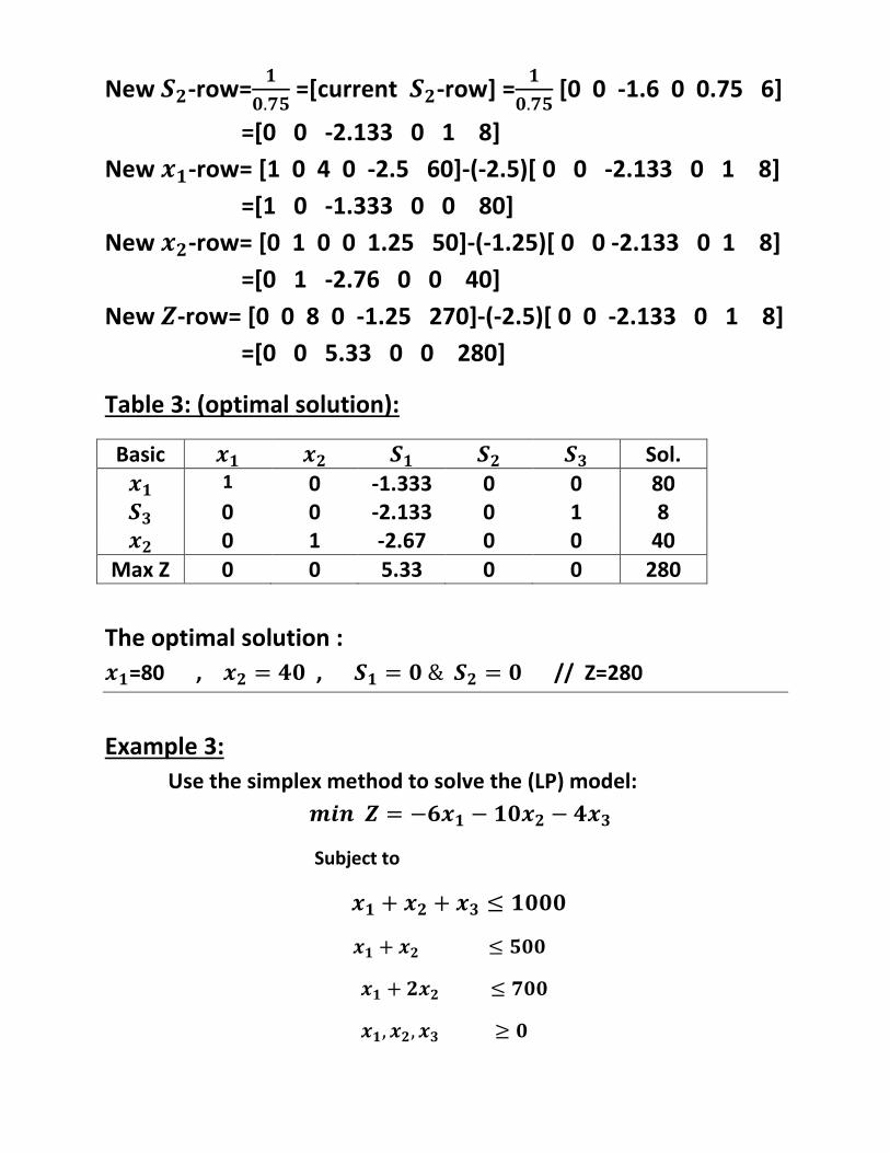
New -row=
=[current -row] =
[0 0 -1.6 0 0.75 6]
=[0 0 -2.133 0 1 8]
New -row= [1 0 4 0 -2.5 60]-(-2.5)[ 0 0 -2.133 0 1 8]
=[1 0 -1.333 0 0 80]
New -row= [0 1 0 0 1.25 50]-(-1.25)[ 0 0 -2.133 0 1 8]
=[0 1 -2.76 0 0 40]
New -row= [0 0 8 0 -1.25 270]-(-2.5)[ 0 0 -2.133 0 1 8]
=[0 0 5.33 0 0 280]
Table 3: (optimal solution):
Basic Sol.
1 0 -1.333 0 0 80 0 0 -2.133 0 1 8 0 1 -2.67 0 0 40
Max Z 0 0 5.33 0 0 280
The optimal solution :
=80 , , // Z=280
Example 3:
Use the simplex method to solve the (LP) model:
Subject to
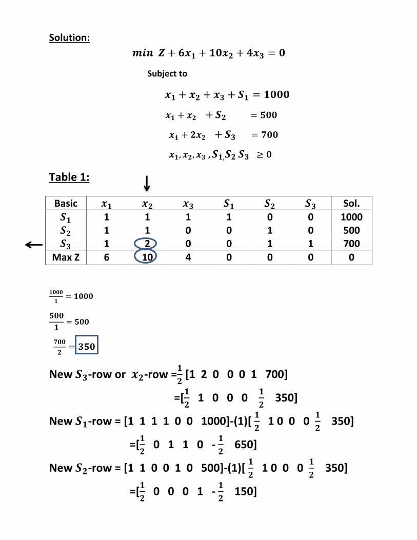
Solution:
Subject to
Table 1:
New -row or -row =
[1 2 0 0 0 1 700]
=[
1 0 0 0
350]
New -row = [1 1 1 1 0 0 1000]-(1)[
1 0 0 0
350]
=[
0 1 1 0 -
650]
New -row = [1 1 0 0 1 0 500]-(1)[
1 0 0 0
350]
=[
0 0 0 1 -
150]
Basic Sol.
1 1 1 1 0 0 1000 1 1 0 0 1 0 500 1 2 0 0 1 1 700
Max Z 6 10 4 0 0 0 0
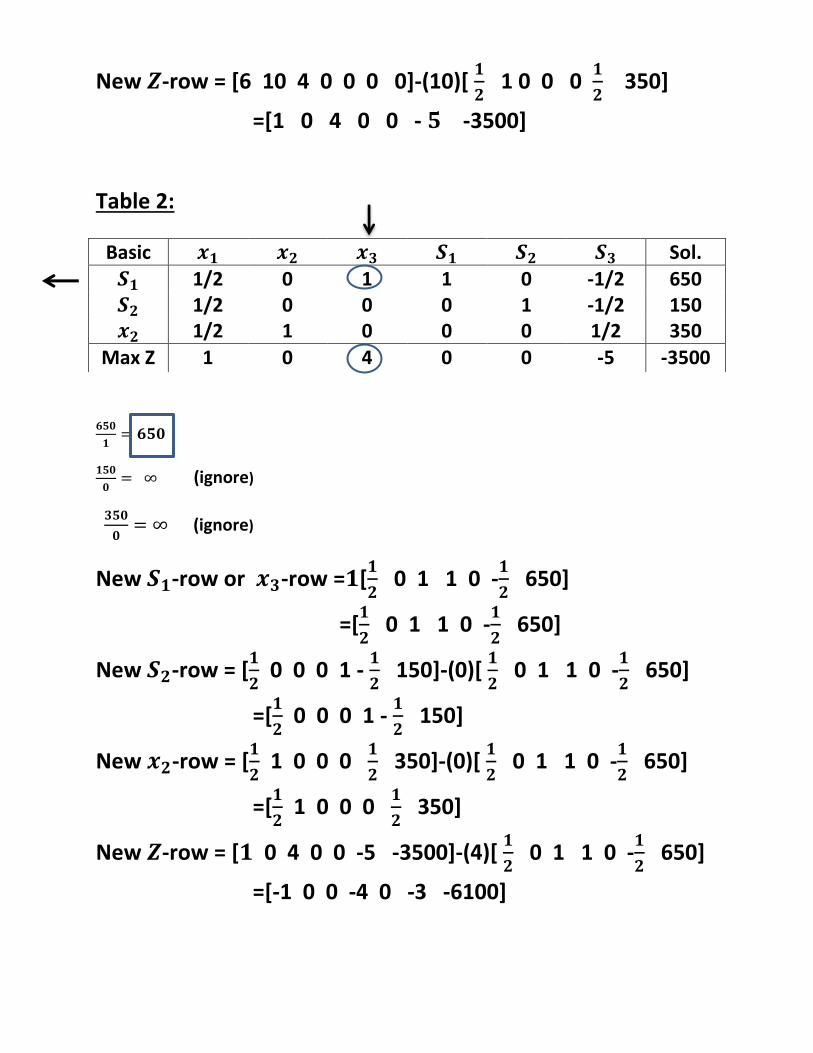
New -row = [6 10 4 0 0 0 0]-(10)[
1 0 0 0
350]
=[1 0 4 0 0 - -3500]
Table 2:
(ignore)
(ignore)
New -row or -row = [
0 1 1 0 -
650]
=[
0 1 1 0 -
650]
New -row = [
0 0 0 1 -
150]-(0)[
0 1 1 0 -
650]
=[
0 0 0 1 -
150]
New -row = [
1 0 0 0
350]-(0)[
0 1 1 0 -
650]
=[
1 0 0 0
350]
New -row = [ 0 4 0 0 -5 -3500]-(4)[
0 1 1 0 -
650]
=[-1 0 0 -4 0 -3 -6100]
Basic Sol.
1/2 0 1 1 0 -1/2 650 1/2 0 0 0 1 -1/2 150 1/2 1 0 0 0 1/2 350
Max Z 1 0 4 0 0 -5 -3500
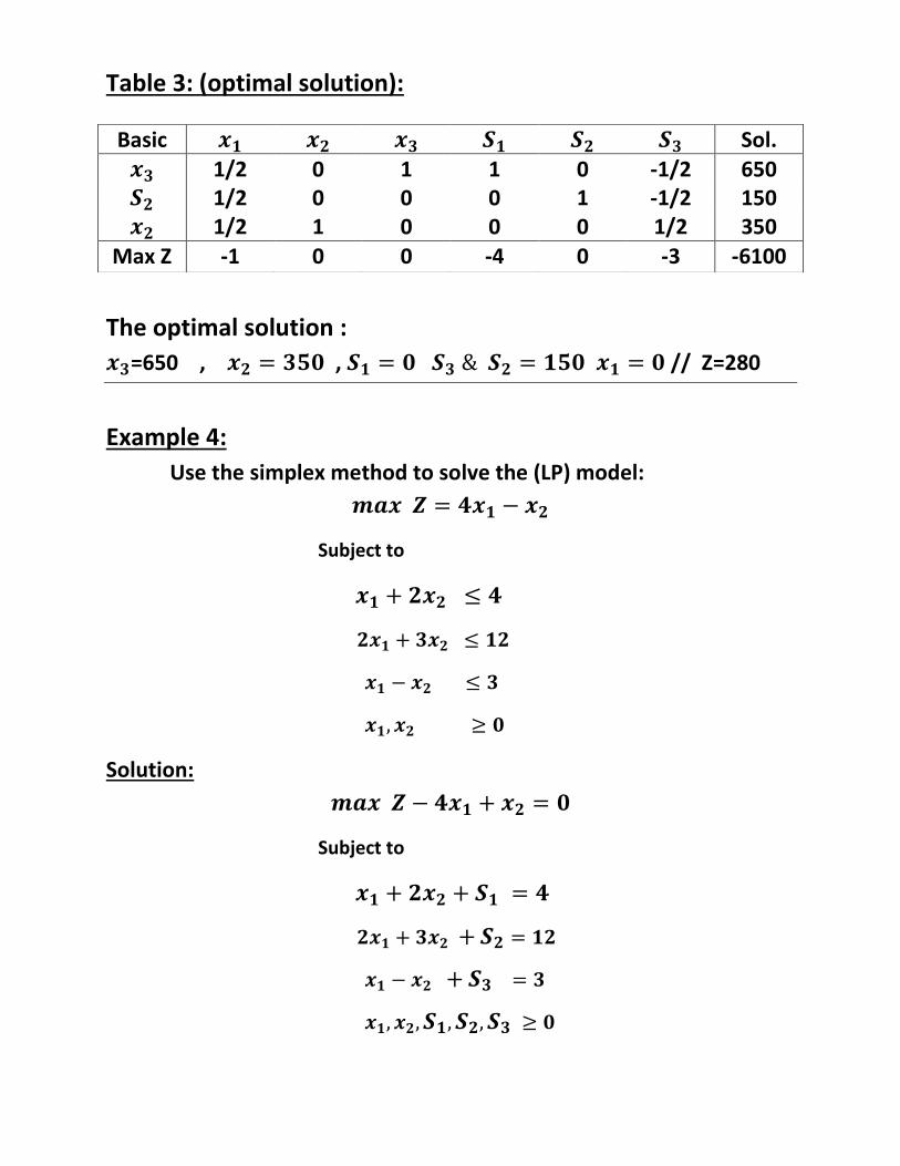
Table 3: (optimal solution):
The optimal solution :
=650 , , // Z=280
Example 4:
Use the simplex method to solve the (LP) model:
Subject to
Solution:
Subject to
Basic Sol.
1/2 0 1 1 0 -1/2 650 1/2 0 0 0 1 -1/2 150 1/2 1 0 0 0 1/2 350
Max Z -1 0 0 -4 0 -3 -6100

Table 1:
New -row or -row = [1 -1 0 0 1 3]
=[1 -1 0 0 1 3]
New -row = [1 2 1 0 0 4]-(1)[ ]
=[0 3 1 0 -1 1]
New -row = [2 3 0 1 0 12]-(2)[ ]
=[0 5 0 1 -2 6]
New -row = [-4 1 0 0 0 0]-(-4)[ ]
=[0 -3 0 0 4 12]
Table 2:
Basic Sol.
1 2 1 0 0 4 2 3 0 1 0 12 1 -1 0 0 1 3
Max Z -4 1 0 0 0 0
Basic Sol.
0 3 1 0 -1 1 0 5 0 1 -2 6 1 -1 0 0 1 3
Max Z 0 -3 0 0 4 12

(ignore)
New -row or -row =
[0 3 1 0 -1 1]
=[0 1 1/3 0 -1/3 1/3]
New -row = [0 5 0 1 -2 6]-(5)[ ]
=[0 0 -2/3 1 11/3 13/3]
New -row = [1 -1 0 0 1 3]-(-1)[ ]
=[1 0 1/3 0 2/3 10/3]
New -row = [0 -3 0 0 4 12]-(-3)[ ]
=[0 0 1 0 3 13]
Table 3: (optimal solution):
The optimal solution :
=10/3 , , // Z=13
Basic Sol.
0 1 1/3 0 -1/3 1/3 0 0 -2/3 1 11/3 13/3 1 0 1/3 0 2/3 10/3
Max Z 0 0 1 0 3 13
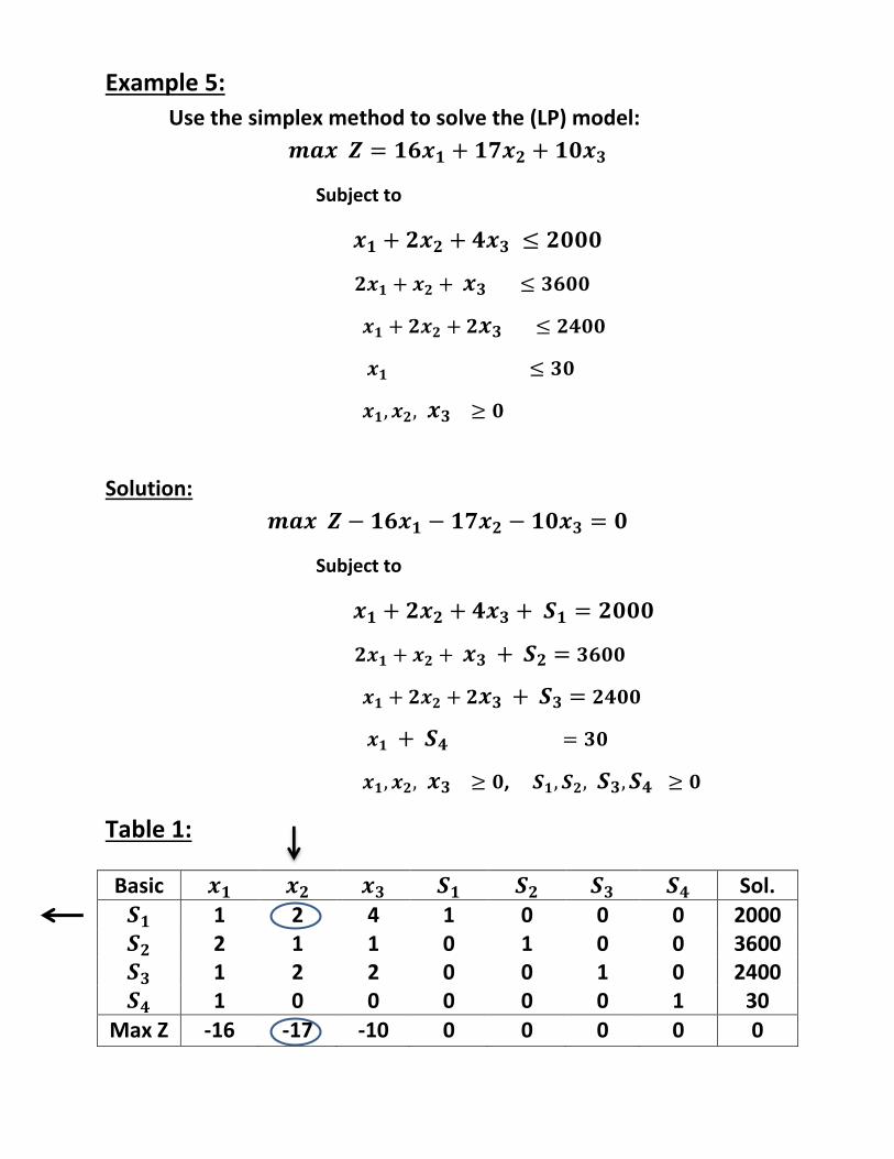
Example 5:
Use the simplex method to solve the (LP) model:
Subject to
Solution:
Subject to
,
Table 1:
Basic Sol.
1 2 4 1 0 0 0 2000 2 1 1 0 1 0 0 3600 1 2 2 0 0 1 0 2400 1 0 0 0 0 0 1 30
Max Z -16 -17 -10 0 0 0 0 0
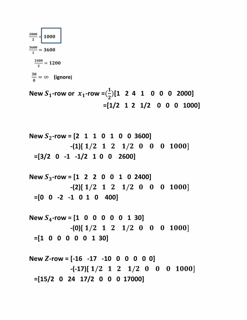
(ignore)
New -row or -row =
[1 2 4 1 0 0 0 2000]
=[1/2 1 2 1/2 0 0 0 1000]
New -row = [2 1 1 0 1 0 0 3600]
-(1)[
=[3/2 0 -1 -1/2 1 0 0 2600]
New -row = [1 2 2 0 0 1 0 2400]
-(2)[
=[0 0 -2 -1 0 1 0 400]
New -row = [1 0 0 0 0 0 1 30]
-(0)[
=[1 0 0 0 0 0 1 30]
New -row = [-16 -17 -10 0 0 0 0 0]
-(-17)[
=[15/2 0 24 17/2 0 0 0 17000]
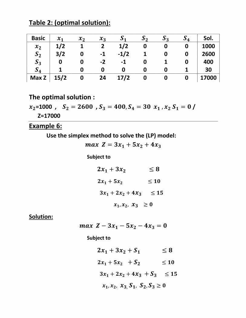
Table 2: (optimal solution):
The optimal solution :
=1000 , , /
Z=17000
Example 6:
Use the simplex method to solve the (LP) model:
Subject to
Solution:
Subject to
Basic Sol.
1/2 1 2 1/2 0 0 0 1000 3/2 0 -1 -1/2 1 0 0 2600 0 0 -2 -1 0 1 0 400 1 0 0 0 0 0 1 30
Max Z 15/2 0 24 17/2 0 0 0 17000
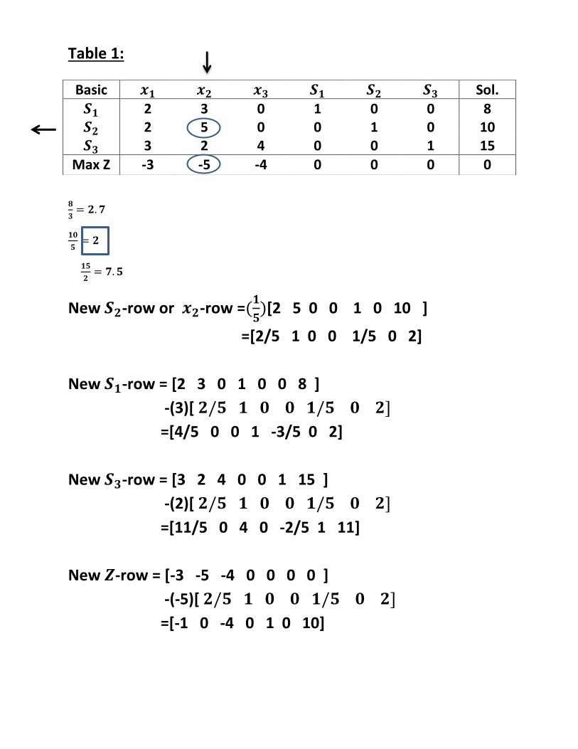
Table 1:
New -row or -row =
[2 5 0 0 1 0 10 ]
=[2/5 1 0 0 1/5 0 2]
New -row = [2 3 0 1 0 0 8 ]
-(3)[
=[4/5 0 0 1 -3/5 0 2]
New -row = [3 2 4 0 0 1 15 ]
-(2)[
=[11/5 0 4 0 -2/5 1 11]
New -row = [-3 -5 -4 0 0 0 0 ]
-(-5)[
=[-1 0 -4 0 1 0 10]
Basic Sol.
2 3 0 1 0 0 8 2 5 0 0 1 0 10 3 2 4 0 0 1 15
Max Z -3 -5 -4 0 0 0 0

Table 2:
New -row or -row =
[11/5 0 4 0 -2/5 1 11]
=[11/20 0 1 0 -1/10 1/4 11/4]
New -row = [4/5 0 0 1 -3/5 0 2 ]
-(0)[
=[4/5 0 0 1 -3/5 0 2]
New -row = [2/5 1 0 0 1/5 0 2 ]
New -row = [-1 0 -4 0 1 0 10 ]
-(-4)[
=[6/5 0 0 0 3/5 1 21]
Table 3: (optimal solution):
The optimal solution :
=2 ,
,
Z=21
,
Basic Sol.
4/5 0 0 1 -3/5 0 2 2/5 1 0 0 1/5 0 2 11/5 1 4 0 -2/5 1 11
Max Z -1 0 -4 0 1 0 10
Basic Sol.
4/5 0 0 1 -3/5 0 2 2/5 1 0 0 1/5 0 2 11/20 0 1 0 -1/10 1/4 11/4
Max Z 6/5 0 0 0 3/5 1 21
View publication statsView publication stats