Anstreicher–Terlaky type monotonic simplex algorithms for linear feasibility problems

Operations Research

Report 2005-03

Anstreicher-Terlaky type

monotonic simplex algorithms

for linear feasibility problems

Bilen Filiz, Zsolt Csizmadia and Tibor Illes

May 2005

Eotvos Lorand University of SciencesDepartment of Operations Research

Copyright c© 2005 Department of Operations Research,Eotvos Lorand University of Sciences,

Budapest, Hungary

ISSN 1215 - 5918

Operations Research Reports No. 2005-03 3

Anstreicher-Terlaky type

monotonic simplex algorithms

for linear feasibility problems

Bilen Filiz, Zsolt Csizmadia and Tibor Illes

Abstract

We define a variant of Anstreicher and Terlaky’s (1994) monotonicbuild-up (MBU) simplex algorithm for linear feasibility problems. Un-der a nondegeneracy assumption weaker than the normal one, the com-plexity of the algorithm can be given by m∆, where ∆ is a constantdetermined by the input data of the problem and m is the number ofconstraints. The constant ∆ cannot be bounded in general by a poly-nomial of the bit length of the input data.

Realizing an interesting property of degeneracy led us to construct anew recursive procedure to handle degenerate problems. The essence ofthis procedure is as follows. If a degenerate pivot tableau is obtained, wedefine a smaller problem, restricting the pivot position to a smaller partof the tableau. On this smaller problem, we follow the same principlesas before to choose the pivot position. The smaller problem is eithersolved completely or a new degenerate subproblem is identified. If thesubproblem was solved then we return to the starting larger problem,where either we can make a nondegenerate pivot, or detect that theproblem is infeasible. It is easy to see that the maximum depth of therecursively embedded subproblems is smaller than 2m.

Upper bounds for the complexities of linear programming version ofMBU and the first phase of the simplex algorithm can be found similarlyunder the nondegeneracy assumption.

Keywords: feasibility problem, Anstreicher-Terlaky type monotonicsimplex algorithms, degeneracy, linear programming.

Mathematics Subject Classification 2000: 90C20.

2005-03-01

4 Bilen Filiz, Zsolt Csizmadia and Tibor Illes

1 Introduction

The first model known in the literature to consider linear inequalities is theFourier mechanical principle, which was also a starting point of the worksof Gyula Farkas. The feasibility issues of linear were investigated by GyulaFarkas [5, 6] in the 19th century. The first known computational method forspecial linear inequality systems was formulated by Fourier. This methodwas generalized to arbitrary linear systems of inequalities by Motzkin, andthis method is known since as Fourier-Motzkin elimination [13].

The analysis of the solution techniques of linear systems of inequalitiesbecome a main issue of linear optimization developed in the middle of the20th century, and is still an interesting research area.

We consider the following feasibility problem

Ax = b, x ≥ 0 (1)

where A ∈ Rm×n,b ∈ R

m. Without loss of generality, we may assume thatrank(A) = m, for the feasibility check of the linear system, and the removalof the redundant equations can be done simultaneously by the Gauss-Jordanelimination. The most well known open question of feasibility problems iswhether there exists a strongly polynomial pivot algorithm for solving (1). Wegive answer to an easier question: we show that a variant of the Anstreicher-Terlaky type monotonic simplex algorithm can be formulated for the problem(1), which has a complexity bound of m∆, where ∆ is a constant determinedby the input data of the problem. Although ∆ is constant, it cannot bebounded by a polynomial of the bit length of the problem, and the analysisis also based on a special nondegeneracy assumption. Our result is new andup to our best knowledge no similar result is known in the literature. In-deed, since the development of Dantzig’s simplex algorithm [3, 4] there wasno pivot algorithm known, that has a complexity bound obtained from theanalysis of the algorithm. Most pivot algorithms starting from a given basismake exponential number of iterations on the Klee-Minty cube [11], or onsome other problem with very similar structure, before obtaining the optimalsolution. For the majority of the pivot algorithms, there are no theoreticalresults concerning the efficiency of the method other than the proof of finite-ness. On the other hand, practical experiences show ([12], page 19) that theaverage number of iterations required to solve a linear programming problemis O(m), where m is the number of constraints of the problem. The practi-cal experience have been supported by many probability based analysis. Inother words, it has been shown that the expected number of iterations of the

Operations Research Reports No. 2005-03

Anstreicher-Terlaky type monotonic simplex algorithms for feasibility problems 5

simplex algorithm is polynomial. We mention the works of Borgwardt [2] andTodd [16]. More information on the topic along with numerous references canbe found in the paper of Fukuda and Terlaky [7].

After Karmarkar’s famous paper [9] on interior point methods, new IPMalgorithms and their analysis became the most popular research area in linearprogramming, pushing the theoretical study and elaboration of new pivotmethods into the background.1 A rare exception is the monotonic built-upsimplex algorithm of Anstreicher and Terlaky [1], that represents a majorinnovation after the former simplex type algorithms. This algorithm has thefollowing main properties: (i) it does not necessarily keep primal feasibilityduring the iterations, (ii) it compares two kinds of pivot positions, (iii) incase of degeneracy it uses some kind of anti-degeneracy rule like minimalindex rule, (iv) if the feasibility of a primal variable is violated it is restoredafter a pivot is made on the so-called leading variable.

In this paper, we define a new algorithm for solving linear feasibility prob-lems following the main idea of the monotonic built-up simplex method ofAnstreicher and Terlaky [1]. We elaborated both the primal and dual ver-sions of our algorithm and both of them have the property that once a variablebecomes feasible, it remains so during the algorithm.

Our choice of pivot position differs from the usual ones from the literaturefor feasibility (linear programming) problems.

We show that our algorithm – under a nondegeneracy assumption – makesat most m∆ iterations before solving the linear feasibility problem. Becausethe fulfillment of the nondegeneracy assumption cannot be known a priori,we introduced a primal-dual recursive version of the algorithm that is capableof solving general degenerate problems without applying any general indexselection rule (as minimal index, lexicographic ordering of variables, etc).

A geometric interpretation of our algorithm is the following. Like thecriss-cross methods, the algorithm generates neighbouring points defined bythe intersection of the constraints – not necessarily feasible basis – of theproblem. If in any iteration the generated point lies on the feasible side ofany defining hyperplane, then any further point generated will lie on the sameside of the hyperplane.

In Section 2, we fix the definitions and notations used.

1The paper of Klee and Minty [11] ended the heroic age of the new pivot algorithms.The new pivot algorithms published afterwards were summarized by Terlaky and Zhang in[15].



In section 3, we define the MBU type simplex method, and prove some ofits important properties. In case of not locally strongly degenerate pivot se-quences, we calculate an upper bound for the complexity of the algorithm. Insection 4, the finiteness of the algorithm is proved without any nondegeneracyassumption. Conclusions close the paper.

2 Definitions and notations

We use the following notations throughout the paper. Scalars and indicesare denoted by small Latin letters, vectors by small boldface Latin letters,matrices by capital Latin letters, and finally index sets by capital calligraphicletters.

For an index set G ⊆ I := {1, 2, . . . , n} and a vector v ∈ Rn, we denote

the subvector of v indexed by G by vG , in other words (vG)i := vi, i ∈ G. Forany matrix T ∈ R

m×n, and index sets F ⊆ J := {1, . . . , m} and G ⊆ I, wedenote the submatrix of T whose rows and columns are indexed by F and G,respectively, by TFG.

Let B ∈ Rm×m be a nonsingular rectangular submatrix of A ∈ R

m×n andN be the matrix consisting of the columns of A not in B. The matrix Bis called a basis of the problem while the index sets IB ⊂ I and IN ⊂ Idenote the index sets of the basic and nonbasic variables, respectively. Itis well known that the corresponding basic solution is given by the formulab := xIB := B−1b, and T = B−1N ∈ R

m×(n−m) defines the short pivottableau corresponding to the basis B. The vector of nonbasic variables isxIN := 0.

For a given basis B, we use the following partition:

IB = I+B ∪ I0

B ∪ I−B ,

where

I+B = {i ∈ IB : xi > 0} , I0

B = {i ∈ IB : xi = 0} and I−B = {i ∈ IB : xi < 0} .

If we want to emphasize the feasibility of a variable xi, we will use thenotation I⊕

B = I+B ∪ I0

B and say that i ∈ I⊕B .

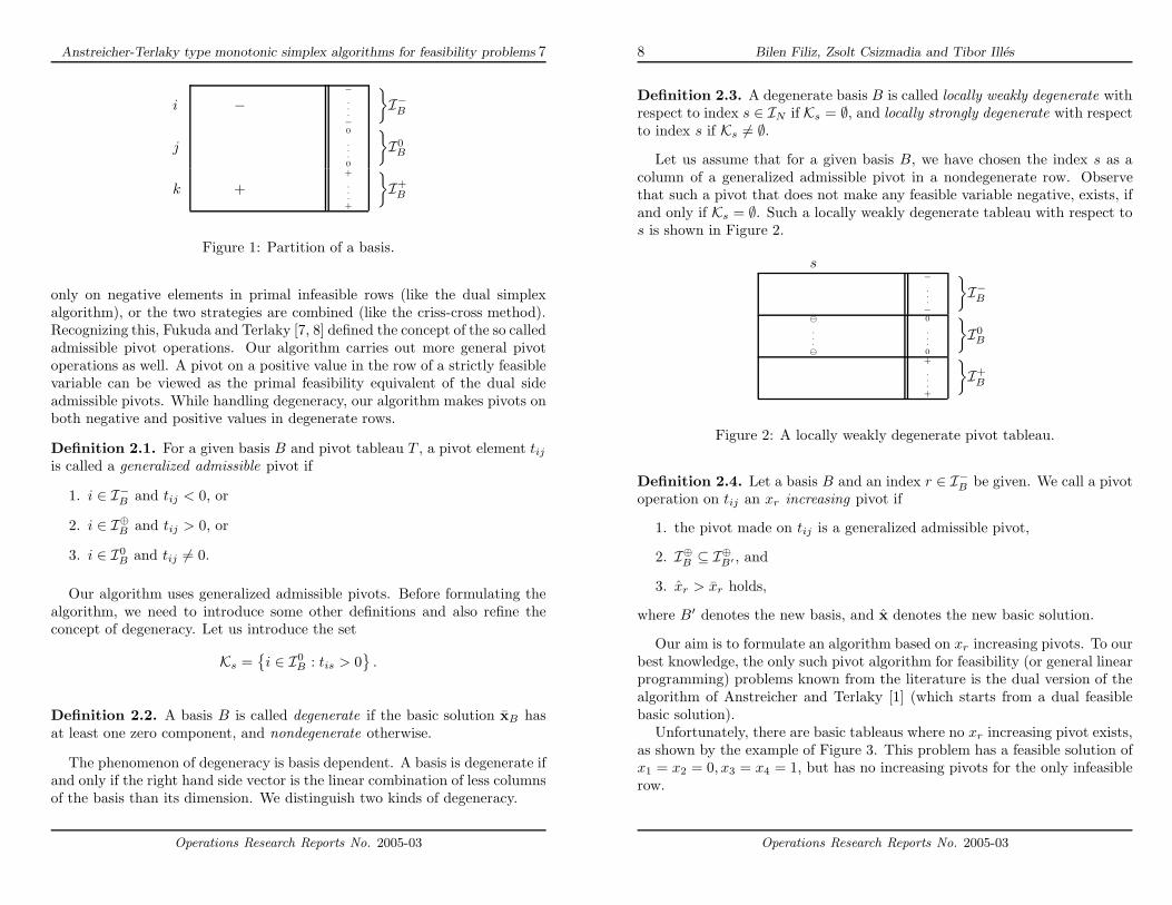
A sample basic tableau according to the above partition is shown in Figure1.

In most pivot algorithms known from the literature pivots are made onlyon positive elements in primal feasible rows (like the simplex algorithm), and



i −−...−

}I−

B

j

0

.

.

.0

}I0

B

k ++

.

.

.+

}I+

B

Figure 1: Partition of a basis.

only on negative elements in primal infeasible rows (like the dual simplexalgorithm), or the two strategies are combined (like the criss-cross method).Recognizing this, Fukuda and Terlaky [7, 8] defined the concept of the so calledadmissible pivot operations. Our algorithm carries out more general pivotoperations as well. A pivot on a positive value in the row of a strictly feasiblevariable can be viewed as the primal feasibility equivalent of the dual sideadmissible pivots. While handling degeneracy, our algorithm makes pivots onboth negative and positive values in degenerate rows.

Definition 2.1. For a given basis B and pivot tableau T , a pivot element tijis called a generalized admissible pivot if

1. i ∈ I−B and tij < 0, or

2. i ∈ I⊕B and tij > 0, or

3. i ∈ I0B and tij �= 0.

Our algorithm uses generalized admissible pivots. Before formulating thealgorithm, we need to introduce some other definitions and also refine theconcept of degeneracy. Let us introduce the set

Ks ={i ∈ I0

B : tis > 0}

.

Definition 2.2. A basis B is called degenerate if the basic solution xB hasat least one zero component, and nondegenerate otherwise.

The phenomenon of degeneracy is basis dependent. A basis is degenerate ifand only if the right hand side vector is the linear combination of less columnsof the basis than its dimension. We distinguish two kinds of degeneracy.



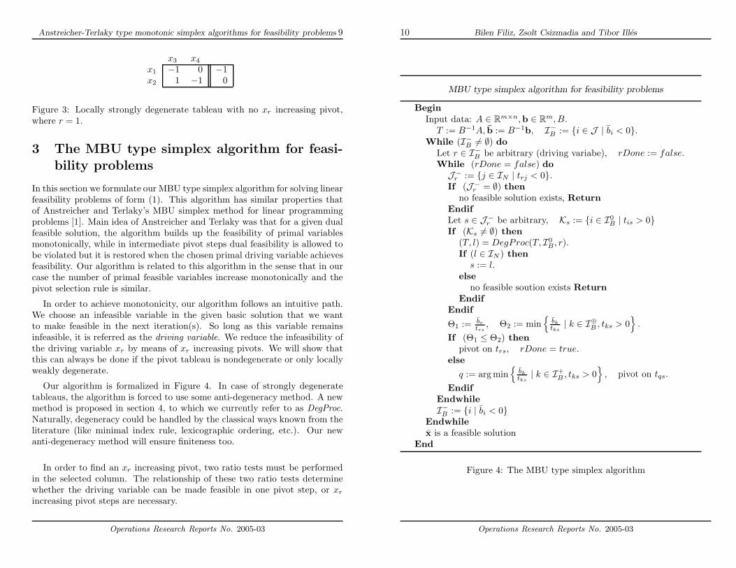
Definition 2.3. A degenerate basis B is called locally weakly degenerate withrespect to index s ∈ IN if Ks = ∅, and locally strongly degenerate with respectto index s if Ks �= ∅.

Let us assume that for a given basis B, we have chosen the index s as acolumn of a generalized admissible pivot in a nondegenerate row. Observethat such a pivot that does not make any feasible variable negative, exists, ifand only if Ks = ∅. Such a locally weakly degenerate tableau with respect tos is shown in Figure 2.

s−...−

}I−

B

�...�

0

.

.

.0

}I0

B

+

.

.

.+

}I+

B

Figure 2: A locally weakly degenerate pivot tableau.

Definition 2.4. Let a basis B and an index r ∈ I−B be given. We call a pivot

operation on tij an xr increasing pivot if

1. the pivot made on tij is a generalized admissible pivot,

2. I⊕B ⊆ I⊕

B′ , and

3. xr > xr holds,

where B′ denotes the new basis, and x denotes the new basic solution.

Our aim is to formulate an algorithm based on xr increasing pivots. To ourbest knowledge, the only such pivot algorithm for feasibility (or general linearprogramming) problems known from the literature is the dual version of thealgorithm of Anstreicher and Terlaky [1] (which starts from a dual feasiblebasic solution).

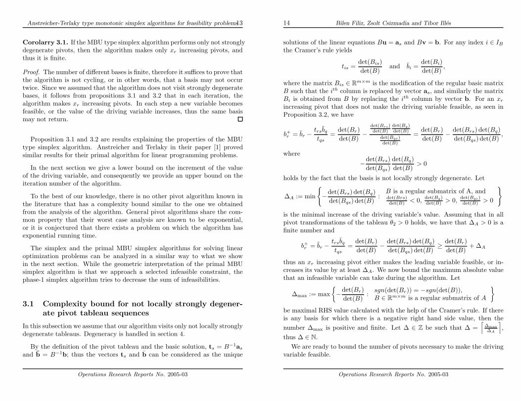
Unfortunately, there are basic tableaus where no xr increasing pivot exists,as shown by the example of Figure 3. This problem has a feasible solution ofx1 = x2 = 0, x3 = x4 = 1, but has no increasing pivots for the only infeasiblerow.



x3 x4

x1 −1 0 −1x2 1 −1 0

Figure 3: Locally strongly degenerate tableau with no xr increasing pivot,where r = 1.

3 The MBU type simplex algorithm for feasi-bility problems

In this section we formulate our MBU type simplex algorithm for solving linearfeasibility problems of form (1). This algorithm has similar properties thatof Anstreicher and Terlaky’s MBU simplex method for linear programmingproblems [1]. Main idea of Anstreicher and Terlaky was that for a given dualfeasible solution, the algorithm builds up the feasibility of primal variablesmonotonically, while in intermediate pivot steps dual feasibility is allowed tobe violated but it is restored when the chosen primal driving variable achievesfeasibility. Our algorithm is related to this algorithm in the sense that in ourcase the number of primal feasible variables increase monotonically and thepivot selection rule is similar.

In order to achieve monotonicity, our algorithm follows an intuitive path.We choose an infeasible variable in the given basic solution that we wantto make feasible in the next iteration(s). So long as this variable remainsinfeasible, it is referred as the driving variable. We reduce the infeasibility ofthe driving variable xr by means of xr increasing pivots. We will show thatthis can always be done if the pivot tableau is nondegenerate or only locallyweakly degenerate.

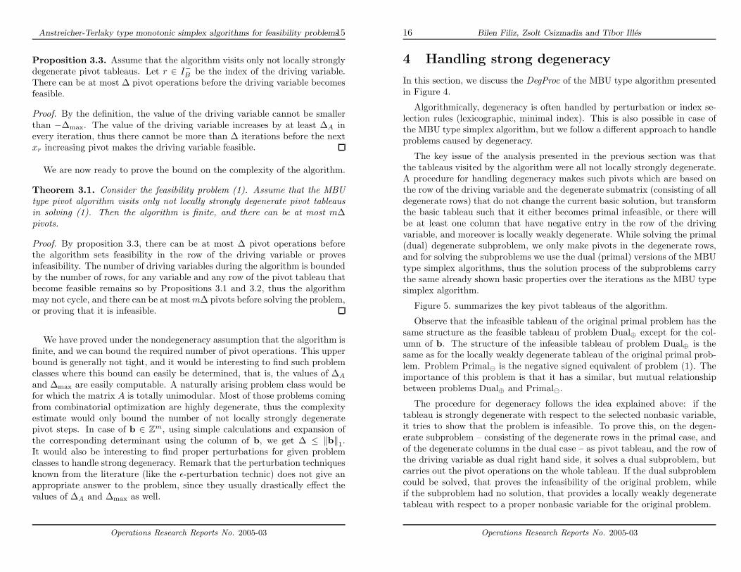
Our algorithm is formalized in Figure 4. In case of strongly degeneratetableaus, the algorithm is forced to use some anti-degeneracy method. A newmethod is proposed in section 4, to which we currently refer to as DegProc.Naturally, degeneracy could be handled by the classical ways known from theliterature (like minimal index rule, lexicographic ordering, etc.). Our newanti-degeneracy method will ensure finiteness too.

In order to find an xr increasing pivot, two ratio tests must be performedin the selected column. The relationship of these two ratio tests determinewhether the driving variable can be made feasible in one pivot step, or xr

increasing pivot steps are necessary.



MBU type simplex algorithm for feasibility problems

BeginInput data: A ∈ R

m×n,b ∈ Rm, B.

T := B−1A, b := B−1b, I−B := {i ∈ J | bi < 0}.

While (I−B �= ∅) do

Let r ∈ I−B be arbitrary (driving variabe), rDone := false.

While (rDone = false) doJ−

r := {j ∈ IN | trj < 0}.If (J−

r = ∅) thenno feasible solution exists, Return

EndifLet s ∈ J−

r be arbitrary, Ks := {i ∈ I0B | tis > 0}

If (Ks �= ∅) then(T, l) = DegProc(T, I0

B, r).If (l ∈ IN ) then

s := l.else

no feasible soution exists ReturnEndif

Endif

Θ1 := br

trs, Θ2 := min

{bk

tks| k ∈ I⊕

B , tks > 0}

.

If (Θ1 ≤ Θ2) thenpivot on trs, rDone = true.

else

q := arg min{

bk

tks| k ∈ I+

B , tks > 0}

, pivot on tqs.Endif

EndwhileI−

B := {i | bi < 0}Endwhilex is a feasible solution

End

Figure 4: The MBU type simplex algorithm


Anstreicher-Terlaky type monotonic simplex algorithms for feasibility problems11

The value of the two ratio tests are denoted by Θ1 and Θ2. From theirdefinition, it is easy to see that Θ1 > 0 and Θ2 ≥ 0. Furthermore, if the basisis not locally strongly degenerate, then Θ2 > 0 holds. The aim of the innercycle of the algorithm is to make the driving variable feasible.

We prove that if the given basis B is not locally strongly degenerate, thenthe algorithm makes only xr increasing pivots. First we investigate the casewhen the driving variable leaves the basis.

Proposition 3.1. For a given basis B, let r ∈ I−B and q ∈ I⊕

B , tqs > 0.Suppose that

bq

tqs= θ2 ≥ θ1 =

br

trs> 0,

where br < 0, trs < 0, bq ≥ 0 and tqs > 0. In this case a pivot is carried outon trs. Let us denote the new basis by B′, then

I⊕B ∪ {s} ⊂ I⊕

B′

holds, thus ∣∣I⊕B′

∣∣ >∣∣I⊕

B

∣∣ .Proof. When trs is the pivot position, the variable xr leaves the basis, whilevariable xs enters it. Let us denote the new basic solution (thus the new righthand side of the pivot tableau) by b+. We distinguish the following cases.

a) For the index s the right hand side becomes b+s = br

trs= θ1 > 0, making

the driving variable x+r = 0 feasible.

b) For i ∈ I+B , i �= s holds that b+

i = bi − tisbr

trs. If tis ≤ 0 then by

using bi ≥ 0, br < 0 and trs < 0 we have b+i > 0, because we add a

nonnegative number to an already positive bi. Otherwise if tis > 0 thenby b+

i = tis

(bi

tis− br

trs

)using the condition bi

tis≥ θ2 ≥ θ1 = br

trs> 0 we

get that b+i > 0.

c) For i ∈ I0B we have b+

i = bi − tis br

trs≥ 0, and by θ2 > 0 either I0

B = ∅ or

tis ≤ 0, thus b+i = − tisbr

trs≥ 0.

As we have seen, no feasible variable becomes infeasible while at least theleaving basic variable xr becomes feasible. It follows that

∣∣I⊕B′∣∣ >

∣∣I⊕B ∣∣.Operations Research Reports No. 2005-03


In the next proposition we investigate the case when a pivot is made outsidethe row of the driving variable. If the basis is not locally strongly degeneratefor the entering nonbasic variable, the pivot made by the algorithm is still xr

increasing.

Proposition 3.2. In a given iteration of the algorithm, for the actual basisB let r ∈ I−

B and q ∈ I⊕B , tqs > 0. Suppose that

0 ≤ bq

tqs= θ2 < θ1 =

br

trs,

where br < 0, trs < 0, bq ≥ 0 and tqs > 0. In this case a pivot is carriedout on tqs. Let us denote the new basis by B′. Then I⊕

B\{q} ⊆ I⊕B′\{s} and

0 > b+r ≥ br. Furthermore, if θ2 > 0, then 0 > b+

r > br holds.

Proof. Using the notations introduced in the previous lemma, we see thatbecause of the ratio test, for any index i ∈ I⊕

B we have i ∈ I⊕B′ if i �= q, as

proved in the previous lemma.Furthermore, b+

s = bq

tqs≥ 0, so s ∈ I⊕B′ thus

I⊕B\{q} ⊆ I⊕

B′\{s}providing that an already feasible variable does not become infeasible. Forthe index of the leading variable b+

r = br− trs bq

tqs, where − trsbq

tqs≥ 0, using that

trs < 0, tqs > 0 and bq ≥ 0. By the condition θ2 < θ1 we have 0 ≥ trs bq

tqs> br

thus

0 > b+r = br − trsbq

tqs≥ br.

If the basis is nondegenerate, or locally weakly degenerate, then θ2 > 0 holdsby definition, so bq

tqs> 0, thus −trs

bq

tqs> 0, and

0 > b+r = br − trs

bq

tqs> br,

finalizing the proof.

Geometrically, Proposition 3.2 can be interpreted as the new solution iscloser to the constraint of the driving variable.

Summarizing Propositions 3.1 and 3.2 we obtain the following result.



Corolarry 3.1. If the MBU type simplex algorithm performs only not stronglydegenerate pivots, then the algorithm makes only xr increasing pivots, andthus it is finite.

Proof. The number of different bases is finite, therefore it suffices to prove thatthe algorithm is not cycling, or in other words, that a basis may not occurtwice. Since we assumed that the algorithm does not visit strongly degeneratebases, it follows from propositions 3.1 and 3.2 that in each iteration, thealgorithm makes xr increasing pivots. In each step a new variable becomesfeasible, or the value of the driving variable increases, thus the same basismay not return.

Proposition 3.1 and 3.2 are results explaining the properties of the MBUtype simplex algorithm. Anstreicher and Terlaky in their paper [1] provedsimilar results for their primal algorithm for linear programming problems.

In the next section we give a lower bound on the increment of the valueof the driving variable, and consequently we provide an upper bound on theiteration number of the algorithm.

To the best of our knowledge, there is no other pivot algorithm known inthe literature that has a complexity bound similar to the one we obtainedfrom the analysis of the algorithm. General pivot algorithms share the com-mon property that their worst case analysis are known to be exponential,or it is conjectured that there exists a problem on which the algorithm hasexponential running time.

The simplex and the primal MBU simplex algorithms for solving linearoptimization problems can be analyzed in a similar way to what we showin the next section. While the geometric interpretation of the primal MBUsimplex algorithm is that we approach a selected infeasible constraint, thephase-1 simplex algorithm tries to decrease the sum of infeasibilities.

3.1 Complexity bound for not locally strongly degener-ate pivot tableau sequences

In this subsection we assume that our algorithm visits only not locally stronglydegenerate tableaus. Degeneracy is handled in section 4.

By the definition of the pivot tableau and the basic solution, ts = B−1as

and b = B−1b; thus the vectors ts and b can be considered as the unique



solutions of the linear equations Bu = as and Bv = b. For any index i ∈ IB

the Cramer’s rule yields

tis =det(Bis)det(B)

and bi =det(Bi)det(B)

,

where the matrix Bis ∈ Rm×m is the modification of the regular basic matrix

B such that the ith column is replaced by vector as, and similarly the matrixBi is obtained from B by replacing the ith column by vector b. For an xr

increasing pivot that does not make the driving variable feasible, as seen inProposition 3.2, we have

b+r = br − trsbq

tqs=

det(Br)det(B)

−det(Brs)det(B)

det(Bq)det(B)

det(Bqs)det(B)

=det(Br)det(B)

− det(Brs) det(Bq)det(Bqs) det(B)

,

where

−det(Brs)det(Bqs)

det(Bq)det(B)

> 0

holds by the fact that the basis is not locally strongly degenerate. Let

∆A := min

{−det(Brs) det(Bq)

det(Bqs) det(B):

B is a regular submatrix of A, anddet(Brs)det(B) < 0,

det(Bq)det(B) > 0, det(Bqs)

det(B) > 0

}

is the minimal increase of the driving variable’s value. Assuming that in allpivot transformations of the tableau θ2 > 0 holds, we have that ∆A > 0 is afinite number and

b+r = br − trsbq

tqs=

det(Br)det(B)

− det(Brs) det(Bq)det(Bqs) det(B)

≥ det(Br)det(B)

+ ∆A

thus an xr increasing pivot either makes the leading variable feasible, or in-creases its value by at least ∆A. We now bound the maximum absolute valuethat an infeasible variable can take during the algorithm. Let

∆max := max{−det(Br)

det(B): sgn(det(Br)) = −sgn(det(B)),

B ∈ Rm×m is a regular submatrix of A

}

be maximal RHS value calculated with the help of the Cramer’s rule. If thereis any basis for which there is a negative right hand side value, then thenumber ∆max is positive and finite. Let ∆ ∈ Z be such that ∆ =

⌈∆max∆A

⌉,

thus ∆ ∈ N.We are ready to bound the number of pivots necessary to make the driving

variable feasible.



Proposition 3.3. Assume that the algorithm visits only not locally stronglydegenerate pivot tableaus. Let r ∈ I−B be the index of the driving variable.There can be at most ∆ pivot operations before the driving variable becomesfeasible.

Proof. By the definition, the value of the driving variable cannot be smallerthan −∆max. The value of the driving variable increases by at least ∆A inevery iteration, thus there cannot be more than ∆ iterations before the nextxr increasing pivot makes the driving variable feasible.

We are now ready to prove the bound on the complexity of the algorithm.

Theorem 3.1. Consider the feasibility problem (1). Assume that the MBUtype pivot algorithm visits only not locally strongly degenerate pivot tableausin solving (1). Then the algorithm is finite, and there can be at most m∆pivots.

Proof. By proposition 3.3, there can be at most ∆ pivot operations beforethe algorithm sets feasibility in the row of the driving variable or provesinfeasibility. The number of driving variables during the algorithm is boundedby the number of rows, for any variable and any row of the pivot tableau thatbecome feasible remains so by Propositions 3.1 and 3.2, thus the algorithmmay not cycle, and there can be at most m∆ pivots before solving the problem,or proving that it is infeasible.

We have proved under the nondegeneracy assumption that the algorithm isfinite, and we can bound the required number of pivot operations. This upperbound is generally not tight, and it would be interesting to find such problemclasses where this bound can easily be determined, that is, the values of ∆A

and ∆max are easily computable. A naturally arising problem class would befor which the matrix A is totally unimodular. Most of those problems comingfrom combinatorial optimization are highly degenerate, thus the complexityestimate would only bound the number of not locally strongly degeneratepivot steps. In case of b ∈ Z

m, using simple calculations and expansion ofthe corresponding determinant using the column of b, we get ∆ ≤ ‖b‖1.It would also be interesting to find proper perturbations for given problemclasses to handle strong degeneracy. Remark that the perturbation techniquesknown from the literature (like the ε-perturbation technic) does not give anappropriate answer to the problem, since they usually drastically effect thevalues of ∆A and ∆max as well.



4 Handling strong degeneracy

In this section, we discuss the DegProc of the MBU type algorithm presentedin Figure 4.

Algorithmically, degeneracy is often handled by perturbation or index se-lection rules (lexicographic, minimal index). This is also possible in case ofthe MBU type simplex algorithm, but we follow a different approach to handleproblems caused by degeneracy.

The key issue of the analysis presented in the previous section was thatthe tableaus visited by the algorithm were all not locally strongly degenerate.A procedure for handling degeneracy makes such pivots which are based onthe row of the driving variable and the degenerate submatrix (consisting of alldegenerate rows) that do not change the current basic solution, but transformthe basic tableau such that it either becomes primal infeasible, or there willbe at least one column that have negative entry in the row of the drivingvariable, and moreover is locally weakly degenerate. While solving the primal(dual) degenerate subproblem, we only make pivots in the degenerate rows,and for solving the subproblems we use the dual (primal) versions of the MBUtype simplex algorithms, thus the solution process of the subproblems carrythe same already shown basic properties over the iterations as the MBU typesimplex algorithm.

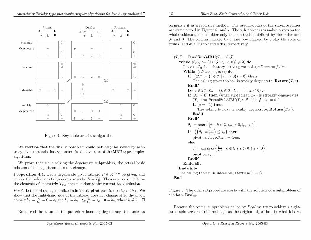
Figure 5. summarizes the key pivot tableaus of the algorithm.

Observe that the infeasible tableau of the original primal problem has thesame structure as the feasible tableau of problem Dual⊕ except for the col-umn of b. The structure of the infeasible tableau of problem Dual⊕ is thesame as for the locally weakly degenerate tableau of the original primal prob-lem. Problem Primal� is the negative signed equivalent of problem (1). Theimportance of this problem is that it has a similar, but mutual relationshipbetween problems Dual⊕ and Primal�.

The procedure for degeneracy follows the idea explained above: if thetableau is strongly degenerate with respect to the selected nonbasic variable,it tries to show that the problem is infeasible. To prove this, on the degen-erate subproblem – consisting of the degenerate rows in the primal case, andof the degenerate columns in the dual case – as pivot tableau, and the row ofthe driving variable as dual right hand side, it solves a dual subproblem, butcarries out the pivot operations on the whole tableau. If the dual subproblemcould be solved, that proves the infeasibility of the original problem, whileif the subproblem had no solution, that provides a locally weakly degeneratetableau with respect to a proper nonbasic variable for the original problem.



Primal Dual ⊕ Primal�Ax = b yT A = cT Ax = bx ≥ 0 y ≥ 0 x ≤ 0

strongly 0 0

degenerate +... + − +

...0 0

− − − 0 . . . 0 − +

⊕ �feasible ⊕ �

......

⊕ ⊕ ⊕ . . . ⊕ �↙↗ ↗↘↙↖

�infeasible ⊕ . . . ⊕ − ... ⊕ . . . ⊕ +

�−

↙↗ ↗↘↙↖weakly � 0 � 0

degenerate...

... ⊕ . . . ⊕ +...

...� 0 � 0− − 0 . . . 0 − − +

Figure 5: Key tableaus of the algorithm

We mention that the dual subproblem could naturally be solved by arbi-trary pivot methods, but we prefer the dual version of the MBU type simplexalgorithm.

We prove that while solving the degenerate subproblem, the actual basicsolution of the algorithm does not change.

Proposition 4.1. Let a degenerate pivot tableau T ∈ Rm×n be given, and

denote the index set of degenerate rows by D = I0B. Then any pivot made on

the elements of submatrix TDI does not change the current basic solution.

Proof. Let the chosen generalized admissible pivot position be tij ∈ TDI. Weshow that the right-hand side of the tableau does not change after the pivot,namely b+

i = bi

tij= 0 = bi and b+

k = bk + tkjbi

tij= bk +0 = bk, where k �= i.

Because of the nature of the procedure handling degeneracy, it is easier to



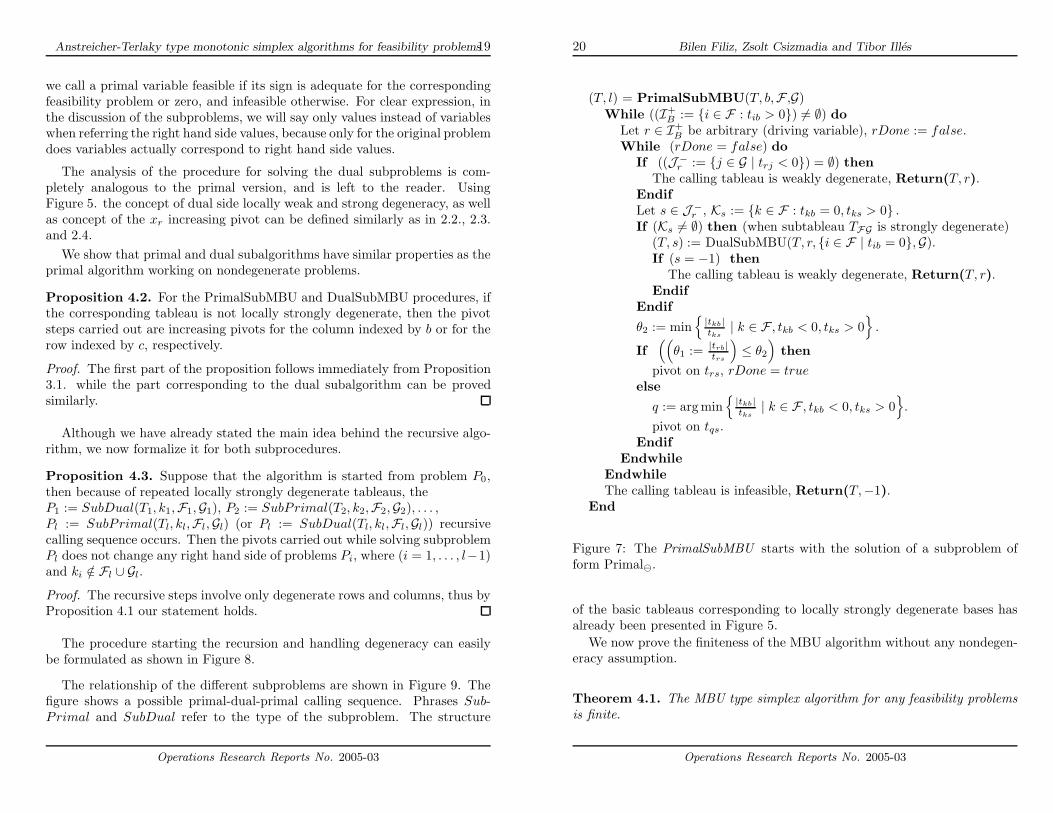
formulate it as a recursive method. The pseudo-codes of the sub-proceduresare summarized in Figures 6. and 7. The sub-procedures makes pivots on thewhole tableaus, but consider only the sub-tableau defined by the index setsF and G. The column indexed by b, and row indexed by c play the roles ofprimal and dual right-hand sides, respectively.

(T, l) = DualSubMBU(T, c,F ,G)While ((J −

B := {j ∈ G : tcj < 0}) �= ∅) doLet r ∈ J −

B be arbitrary (driving variable), rDone := false.While (rDone = false) do

If ((I+r := {i ∈ F | tir > 0}) = ∅) then

The calling pivot tableau is weakly degenerate, Return(T, r).EndifLet s ∈ I+

r , Ks = {k ∈ G | tck = 0, tsk < 0} .If (Ks �= ∅) then (when subtableau TFG is strongly degenerate)

(T, s) := PrimalSubMBU(T, r,F , {j ∈ G | tcj = 0}).If (s = −1) then

The calling tableau is weakly degenerate, Return(T, r).Endif

Endif

θ2 := max{

tck

tsr| k ∈ G, tck > 0, tsk < 0

}If

((θ1 := tcr

tsr

)≤ θ2

)then

pivot on tsr, rDone = true.else

q := arg max{

tck

tsr| k ∈ G, tck > 0, tsk < 0

}.

pivot on tsq.Endif

EndwhileEndwhileThe calling tableau is infeasible, Return(T,−1).

End

Figure 6: The dual subprocedure starts with the solution of a subproblem ofthe form Dual⊕.

Because the primal subproblems called by DegProc try to achieve a right-hand side vector of different sign as the original algorithm, in what follows



we call a primal variable feasible if its sign is adequate for the correspondingfeasibility problem or zero, and infeasible otherwise. For clear expression, inthe discussion of the subproblems, we will say only values instead of variableswhen referring the right hand side values, because only for the original problemdoes variables actually correspond to right hand side values.

The analysis of the procedure for solving the dual subproblems is com-pletely analogous to the primal version, and is left to the reader. UsingFigure 5. the concept of dual side locally weak and strong degeneracy, as wellas concept of the xr increasing pivot can be defined similarly as in 2.2., 2.3.and 2.4.

We show that primal and dual subalgorithms have similar properties as theprimal algorithm working on nondegenerate problems.

Proposition 4.2. For the PrimalSubMBU and DualSubMBU procedures, ifthe corresponding tableau is not locally strongly degenerate, then the pivotsteps carried out are increasing pivots for the column indexed by b or for therow indexed by c, respectively.

Proof. The first part of the proposition follows immediately from Proposition3.1. while the part corresponding to the dual subalgorithm can be provedsimilarly.

Although we have already stated the main idea behind the recursive algo-rithm, we now formalize it for both subprocedures.

Proposition 4.3. Suppose that the algorithm is started from problem P0,then because of repeated locally strongly degenerate tableaus, theP1 := SubDual(T1, k1,F1,G1), P2 := SubPrimal(T2, k2,F2,G2), . . . ,Pl := SubPrimal(Tl, kl,Fl,Gl) (or Pl := SubDual(Tl, kl,Fl,Gl)) recursivecalling sequence occurs. Then the pivots carried out while solving subproblemPl does not change any right hand side of problems Pi, where (i = 1, . . . , l−1)and ki /∈ Fl ∪ Gl.

Proof. The recursive steps involve only degenerate rows and columns, thus byProposition 4.1 our statement holds.

The procedure starting the recursion and handling degeneracy can easilybe formulated as shown in Figure 8.

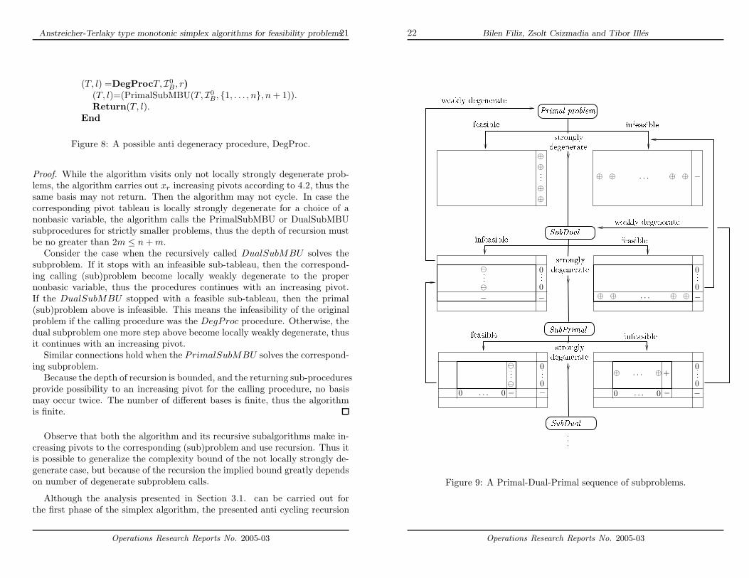
The relationship of the different subproblems are shown in Figure 9. Thefigure shows a possible primal-dual-primal calling sequence. Phrases Sub-Primal and SubDual refer to the type of the subproblem. The structure



(T, l) = PrimalSubMBU(T, b,F ,G)While ((I+

B := {i ∈ F : tib > 0}) �= ∅) doLet r ∈ I+

B be arbitrary (driving variable), rDone := false.While (rDone = false) do

If ((J −r := {j ∈ G | trj < 0}) = ∅) then

The calling tableau is weakly degenerate, Return(T, r).EndifLet s ∈ J −

r , Ks := {k ∈ F : tkb = 0, tks > 0} .If (Ks �= ∅) then (when subtableau TFG is strongly degenerate)

(T, s) := DualSubMBU(T, r, {i ∈ F | tib = 0},G).If (s = −1) then

The calling tableau is weakly degenerate, Return(T, r).Endif

Endif

θ2 := min{

|tkb|tks

| k ∈ F , tkb < 0, tks > 0}

.

If((

θ1 := |trb|trs

)≤ θ2

)then

pivot on trs, rDone = trueelse

q := arg min{

|tkb|tks

| k ∈ F , tkb < 0, tks > 0}.

pivot on tqs.Endif

EndwhileEndwhileThe calling tableau is infeasible, Return(T,−1).

End

Figure 7: The PrimalSubMBU starts with the solution of a subproblem ofform Primal�.

of the basic tableaus corresponding to locally strongly degenerate bases hasalready been presented in Figure 5.

We now prove the finiteness of the MBU algorithm without any nondegen-eracy assumption.

Theorem 4.1. The MBU type simplex algorithm for any feasibility problemsis finite.



(T, l) =DegProcT, I0B, r)

(T, l)=(PrimalSubMBU(T, I0B, {1, . . . , n}, n + 1)).

Return(T, l).End

Figure 8: A possible anti degeneracy procedure, DegProc.

Proof. While the algorithm visits only not locally strongly degenerate prob-lems, the algorithm carries out xr increasing pivots according to 4.2, thus thesame basis may not return. Then the algorithm may not cycle. In case thecorresponding pivot tableau is locally strongly degenerate for a choice of anonbasic variable, the algorithm calls the PrimalSubMBU or DualSubMBUsubprocedures for strictly smaller problems, thus the depth of recursion mustbe no greater than 2m ≤ n + m.

Consider the case when the recursively called DualSubMBU solves thesubproblem. If it stops with an infeasible sub-tableau, then the correspond-ing calling (sub)problem become locally weakly degenerate to the propernonbasic variable, thus the procedures continues with an increasing pivot.If the DualSubMBU stopped with a feasible sub-tableau, then the primal(sub)problem above is infeasible. This means the infeasibility of the originalproblem if the calling procedure was the DegProc procedure. Otherwise, thedual subproblem one more step above become locally weakly degenerate, thusit continues with an increasing pivot.

Similar connections hold when the PrimalSubMBU solves the correspond-ing subproblem.

Because the depth of recursion is bounded, and the returning sub-proceduresprovide possibility to an increasing pivot for the calling procedure, no basismay occur twice. The number of different bases is finite, thus the algorithmis finite.

Observe that both the algorithm and its recursive subalgorithms make in-creasing pivots to the corresponding (sub)problem and use recursion. Thus itis possible to generalize the complexity bound of the not locally strongly de-generate case, but because of the recursion the implied bound greatly dependson number of degenerate subproblem calls.

Although the analysis presented in Section 3.1. can be carried out forthe first phase of the simplex algorithm, the presented anti cycling recursion



+

⊕⊕ ⊕ ⊕

⊕⊕

⊕⊕

⊕⊕

⊕⊕ ⊕ ⊕

. . .

. . . . . .

. . .

. . .

��

��

��

��

��

��

− − −

− − − −

−

�

�

�

�

��

��

��

��

��

��

��

0

0

0

0

0 0

0

00 0

0

0

��

��

��

��

��

��

��

��

��

��

��

��

Figure 9: A Primal-Dual-Primal sequence of subproblems.



procedure cannot be naturally applied for the simplex algorithm. The mainreason for this is that when a subproblem is feasible, we greatly make use ofthe infeasibility of the driving variable to reach the conclusion that the callingproblem is infeasible.

4.1 Algorithm variants

As already stated, it would be possible to solve the degenerate subproblemswith an arbitrary pivot method, similarly like in the case of the Hungarianmethod for linear programming [10], in which the criss-cross method was used[14].

In practice, the efficiency of the algorithm could be increased if the choiceof the driving variable as well as the choice of the variable to enter the basiswould not be arbitrary, although this freedom may help in case of numericallybad problems.

The most expensive operation of the pivot methods is the calculation ofthe updated pivot row and column. However, for an efficient choice of pivotposition, it could be interesting to look for locally weakly degenerate columnsfor the driving variable. Similarly, it may happen that on a pivot tableauthere are infeasible variables that could be made feasible in only one step, butanother one would require even recursion.

If we know a greater part of the pivot tableau, it may be worth to checkfor possible change of the driving variable. If in any step the pivot tableauis locally strongly degenerate for the selected driving variable, it may as wellhappen that there is an infeasible variable that could be made feasible whilepreserving the monotonicity of the cardinality of the feasible variables. Sucha pivot would preserve the finiteness of the algorithm.

It must be noted however, that unfortunately in some cases neither of thesestrategies can be used, and recursion is necessary, like in the example of Figure3.

5 Conclusion

We introduced a new MBU type simplex algorithm for linear feasibility prob-lems, and presented a new anti-degeneracy procedure. The same analysis canbe made for the first phase of the primal simplex algorithm, and the origi-nal MBU simplex algorithm under the assumption that the tableaus visitedare not strongly degenerate. The presented anti-degeneracy procedure uses



the special structure of the MBU type simplex algorithm, therefore is notapplicable for the simplex method.

The anti-degeneracy rule is new, and differs from the known methods fromthe literature. The new complexity analysis of the algorithm proves to bemore interesting for locally weakly degenerate pivot sequences, and is verysensitive to perturbation. It would be interesting to find perturbations thatfit to the presented anti-degeneracy method.

References

[1] Anstreicher, K. M. and Terlaky T., A Monotonic Build-Up Simplex Al-gorithm for Linear Programming. Operations Research 42:556-561, 1994.

[2] Borgwardt, K. H., The Simplex Method: A Probabilistic Analysis. Algo-rithms and Combinatorics, Vol. 1, Springer, Berlin, 1987.

[3] Dantzig, G.B., Programming in a Linear Structure. Comptroller, USAF,Washington D.C., 1948.

[4] Dantzig, G.B., Linear Programming and Extensions. Princeton Univer-sity Press, Princeton, New Jersey, 1963.

[5] Farkas Gy., A Fourier-fele mechanikai elv alkalmazasai. Mathematikai esTermeszettudomanyi Ertesıto, 12:457-472, 1894.

[6] Farkas Gy., A Fourier-fele mechanikai elv alkalmazasainak algebraialapjarol. Mathematikai es Physikai Lapok 5:49-54, 1896.

[7] Fukuda K. and Terlaky T., Criss-cross methods: A fresh view on pivotalgorithms. Mathematical Programming 79:369-395, 1997.

[8] Fukuda K. and Terlaky T., On the existence of a short admissible pivotsequence for feasibility and linear optimization problems. Pure Mathe-matics with Applications 10 no. 4, 431-447, 1999.

[9] Karmarkar, N., A new polynomial-time algorithm for linear program-ming. Combinatorica 4:373-395, 1984.

[10] Klaszky, E., Terlaky, T., Magyar modszer tıpusu algoritmusok lineerisprogramozasi feladatok megoldasara. Alkalmazott Matematikai Lapok12, 1-14, 1986.



[11] Klee, V. and Minty, G.J., How good is the simplex algorithm? InO. Shisha, editor, Inequalities III, Academic Press, New York, 1972.

[12] Maros I., Computational Techniques of the Simplex Method. Kluwer Aca-demic Publishers, Boston, 2003.

[13] Prekopa A., On the development of optimization. American Mathemati-cal Monthly, 87:527–542, 1980.

[14] Terlaky, T., A convergent criss-cross method, Mathematische Opera-tionsforschung und Statistik Series Optimization , Vol. 16, No. 5, 683-690,1985.

[15] Terlaky T. and Zhang S., Pivot rules for linear programming: A survey onrecent theoretical developments. Annals of Operations Research 46:203-233, 1993.

[16] Todd, M. J., Polynomial expected behavior of a pivoting algorithm forlinear complementarity and linear programming problems. MathematicalProgramming 35:173-192, 1986.

Zsolt Csizmadia, Tibor IllesEotvos Lorand University, Department of Operations ResearchH- 1117 Budapest, Pazmany Peter setany 1/C.E-mail: [email protected], [email protected]

Filiz BilenEastern Mediterranean University, Department of MathematicsFamagusta, North-CyprusE-mail: [email protected]




Earlier Research Reports

1991-01 T. Illes, J. Mayer and T. Terlaky: A new approach to thecolour matching problem

1991-02 E. Klaszky, J. Mayer and T. Terlaky: A geometric program-ming approach to the chanel capacity problem

1992-01 Edvi T.: Karmarkar projektıv skalazasi algoritmusa

1992-02 Kassay G.: Minimax tetelek es alkalmazasaik

1992-03 T. Illes, I. Joo and G. Kassay: On a nonconvex Farkas theoremand its applications in optimization theory

1992-04 Interior point methods. Proceedings of the IPM 93. Work-

shop jan. 5. 1993

Recent Operations Research Reports

2003-01 Zsolt Csizmadia and Tibor Illes: New criss-cross type algo-rithms for linear complementarity problems with sufficient matrices

2003-02 Tibor Illes and Adam B. Nagy: A sufficient optimality criteriafor linearly constrained, separable concave minimization problems

2004-01 Tibor Illes and Marianna Nagy: The Mizuno–Todd–Ye predictor–corrector algorithm for sufficient matrix linear complementarity problem

2005-01 Miklos Ujvari: On a closedness theorem

2005-02 Falukozy Tamas es Vizvari Bela: Az arutozsde gabona szekciojanakarvarakozasai a kukorica kereskedesenek tukreben

2005-03 Bilen Filiz, Zsolt Csizmadia and Tibor Illes : Anstreicher-Terlaky type monotonic simplex algorithms for linear feasibility prob-lems

Anstreicher–Terlaky type monotonic simplex algorithms for linear feasibility problems

Documents

Transcript of Anstreicher–Terlaky type monotonic simplex algorithms for linear feasibility problems