arX

iv:0

711.

3921

v2 [

cond

-mat

.str

-el]

28

Nov

200

7

Simplex solid states of SU(N) quantum antiferromagnets

Daniel P. ArovasDepartment of Physics, University of California at San Diego, La Jolla, CA 92093

(Dated: February 19, 2013)

I define a set of wavefunctions for SU(N) lattice antiferromagnets, analogous to the valence bondsolid states of Affleck et al. [1], in which the singlets are extended over N-site simplices. As with thevalence bond solids, the new simplex solid (SS) states are extinguished by certain local projectionoperators, allowing one to construct Hamiltonians with local interactions which render the SS statesexact ground states. Using a coherent state representation, I show that the quantum correlations ineach SS state are calculable as the finite temperature correlations of an associated classical model,with N-spin interactions, on the same lattice. In three and higher dimensions, the SS states canspontaneously break SU(N) and exhibit N-sublattice long-ranged order, as a function of a discreteparameter which fixes the local representation of SU(N). I analyze this transition using a classicalmean field approach. For N > 2 the ordered state is selected via an ‘order by disorder’ mechanism.As in the AKLT case, the bulk representations fractionalize at an edge, and the ground state entropyis proportional to the volume of the boundary.

PACS numbers: 75.10.Hk, 75.10.Jm

I. INTRODUCTION

At the classical level, the thermodynamic propertiesof ferromagnets and antiferromagnets are quite similar.Both states break certain internal symmetries, whetherthey be discrete or continuous, and often crystalline pointgroup symmetries as well. Antiferromagnetism holds theinteresting possibility of frustration, which can lead tocomplex behavior even at the classical level.

Quantum mechanics further distinguishes antiferro-magnetism as the more interesting of the two phenom-ena. Quantum fluctuations compete with classical order-ing, and many models of quantum antiferromagnetismremain disordered even in their ground states. The rea-son is that on the local level, quantum antiferromagnetsprefer distinctly non-classical correlations, in that theyform singlets, which are superpositions of classical states.For a S = 1

2 Heisenberg antiferromagnet on a bipartitelattice, theorems by Marshall [2] and by Lieb and Mattis[3] rigorously prove that the ground state is a total spin

singlet: Stot = 0. Any total singlet can be expanded in a(nonorthogonal) basis of valence bonds, which are singlet

pairs (ij) ≡ 2−1/2(∣

∣↑i ↓j

⟩

−∣

∣↓i ↑j

⟩)

extending betweensites i and j. The most probable singlets are betweennearest neighbors, which thereby take full advantage of

the Heisenberg interaction J Si · Sj and achieve a mini-

mum possible energy ε0 = − 34 J for that particular link.

Taking linear combinations of such states lowers the en-ergy, via delocalization, with respect to any fixed singletconfiguration; this is the basic idea behind Anderson’scelebrated resonating valence bond (RVB) picture [4]. Ifone allows the singlet bonds to be long-ranged, such astate can even possess classical Neel order [5].

Taking advantage of quantum singlets, one canconstruct correlated quantum-disordered wavefunctionswhich are eigenstates of local projection operators. Thisfeature allows one to construct a many-body Hamiltonian

which renders the parent wavefunction an exact groundstate, typically with a gap to low-energy excitations. Per-haps the simplest example is the Majumdar-Ghosh (MG)model for a S = 1

2 spin-chain [6], the parent state ofwhich is given by alternating singlet bonds, viz.

∣

∣Ψ⟩

=∣

∣ · · · • • • • • • · · ·⟩

(1)

The key feature to∣

∣Ψ⟩

is that any consecutive trio ofsites (n, n+ 1, n+ 2) can only be in a state of total spinS = 1

2 – there is no S = 32 component. Thus,

∣

∣Ψ⟩

is aneigenstate of the projection operator

P3/2(n, n+1, n+2) = − 14 + 1

3

(

Sn +Sn+1 +Sn+2

)2(2)

with zero eigenvalue, and an exact ground state for

H = J∑

n P3/2(n, n + 1, n + 2). As∣

∣Ψ⟩

breaks lat-

tice translation symmetry, a second (degenerate) groundstate follows by shifting

∣

∣Ψ⟩

by one lattice spacing. Ex-tensions of the MG model to higher dimensions and tohigher spin, where the ground state is again of the Kekuleform, i.e. a product of local valence bond singlets, werediscussed by Klein [7].

Another example is furnished by the valence bondsolid (VBS) states of Affleck, Kennedy, Lieb, and Tasaki(AKLT) [1]. The general AKLT state is compactly writ-ten in terms of Schwinger boson operators [8]:

∣

∣Ψ(L ; M)⟩

=∏

〈ij〉

(

b†i↑ b†j↓ − b†i↓ b

†j↑)M ∣

∣ 0⟩

, (3)

which assigns m singlet creation operators to each linkof a lattice L. The total boson occupancy on each site iszM , where z is the lattice coordination number; in theSchwinger representation this corresponds to 2S. Thus, adiscrete family of AKLT states with S = 1

2zM is definedon each lattice, where M is any integer. The maximumtotal spin on any link is then Smax

ij = 2S −M , and anyHamiltonian constructed out of link projectors for total

2

spin S ∈[

2S −M + 1 , 2S]

, with positive coefficients,

renders∣

∣Ψ(L ; M)⟩

an exact zero energy ground state.The elementary excitations in these states were treatedusing a single mode approximation (SMA) in ref. [8].

The ability of two spins to form a singlet state is a spe-cial property of the group SU(2). Decomposing the prod-uct of two spin-S representations yields the well-knownresult,

S ⊗ S = 0 ⊕ 1 ⊕ 2 ⊕ · · · ⊕ 2S , (4)

and there is always a singlet available. If we replaceSU(2) by SU(3), this is no longer the case. The repre-sentations of SU(N) are classified by (N − 1)-row Young

tableaux (l1, l2, . . . , lN−1) with lj boxes in row j, and

with l1 ≥ l2 ≥ · · · ≥ lN−1. The product of two funda-mental (1, 0) representations of SU(3) is

3

⊗3

=

3

⊕6

, (5)

which does not contain a singlet. One way to rescue thetwo-site singlet, for general SU(N), is to take the productof the fundamental representation N with the antifun-damental N . This yields a singlet plus the (N2 − 1)-dimensional adjoint representation. In this manner, gen-eralizations of the SU(2) antiferromagnet can be definedin such a manner that the two-site valence bond structureis preserved, but only on bipartite lattices [9, 10].

Another approach is to keep the same representationof SU(N) on each site, but to create SU(N) singlets ex-tending over multiple sites. When each site is in thefundamental representation, one creates N -site singlets,

ǫα1...αN b†

α1

(i1) · · · b†αN

(iN )∣

∣ 0⟩

, (6)

where b†α(i) creates a Schwinger boson of flavor index αon site i. The SU(N) spin operators may be written interms of the Schwinger bosons as

Sαβ = b†α bβ − p

Nδαβ , (7)

with Tr (S) = 0, for the general symmetric (p, 0) repre-sentation. These satisfy the SU(N) commutation rela-tions,

[

Sαβ , S

µν

]

= δβµ Sαν − δαν S

βµ . (8)

Extended valence bond solid (XVBS) states were firstdiscussed by Affleck et al. in ref. [11]. In that work,SU(2N) states where N = mz were defined on lattices ofcoordination number z, with singlets extending over z+1sites. Like the MG model, the XVBS states break lat-tice translation symmetry t and their ground states aredoubly degenerate; they also break a charge conjugationsymmetry C, preserving the product t C. In addition toSMA magnons, the XVBS states were found to exhibitsoliton excitations interpolating between the degenerate

vacua. More recently, Greiter and Rachel [12] consideredSU(N) valence bond spin chains in both the fundamentaland other representations, constructing their correspond-ing Hamiltonians, and discussing soliton excitations. Ex-tensions of Klein models, with Kekule ground states con-sisting of products of local SU(N) singlets, were discussedby Shen [13], and more recently by Nussinov and Ortiz[14]. An SU(4) model on a two leg ladder with with adoubly degenerate Majumdar-Ghosh type ground statehas been discussed by Chen et al. [15].

Shen also discussed a generalization of Anderson’sRVB state to SU(N) spins, as a prototype of a spin-orbit liquid state [13]. A more clearly defined and well-analyzed model was recently put forward by Pankov,Moessner, and Sondhi [16], who generalized the Rokhsar-Kivelson quantum dimer model [17] to a model of res-onating singlet valence plaquettes. Their plaquettes areN -site SU(N) singlets (N = 3 and N = 4 modelswere considered), which resonate under the action of theSU(N) antiferromagnetic Heisenberg Hamiltonian, pro-jected to the valence plaquette subspace. The models andstates considered here do not exhibit this phenomenonof resonance. Rather, they are described by static “sin-glet valence simplex” configurations. Consequently, theirphysics is quite different, and in fact simpler. For exam-ple, with resonating valence bonds or plaquettes, one can

introduce vison excitations [18] which are Z2 vortex ex-citations, changing the sign of the bonds or plaquetteswhich are crossed by the vortex string [19]. For simplex(or plaquette) solids, there is no resonance, and the visondoes not create a distinct quantum state. The absence of‘topological quantum order’ in Klein and AKLT modelshas been addressed by Nussinov and Ortiz [14].

Here I shall explore further generalizations of theAKLT scheme, describing a family of ‘simplex solid’ (SS)states on N -partite lattices. While the general AKLTstate is written as a product over the links of a lattice L,with M singlet creation operators applied to a given link,the SS states, mutatis mutandis , apply M SU(N) singletoperators on each N -simplex. Each site then containsan SU(N) spin whose representation is determined byM and the lattice coordination. Furthermore, as is thecase with the AKLT states, the SS states admit a simplecoherent state description in terms of classical CPN−1

vectors. Their equal-time quantum correlations are thencomputable as the finite temperature correlations of anassociated classical model on the same lattice. A classicalordering transition in this model corresponds to a zero-temperature quantum critical point as a function of M(which is, however, a discrete parameter). I argue thatthe ordered SS states select a particular ordered struc-ture via an ‘order by disorder’ mechanism. Finally, Idiscuss what happens to these states at an edge, wherethe bulk SU(N) representation is effectively fractional-ized, and a residual entropy proportional to the volumeof the boundary arises.

3

II. SIMPLEX SOLIDS

Consider an N -site simplex Γ , and define the SU(N)singlet creation operator

R†Γ = ǫα1...α

N b†α1

(Γ1) · · · b†αN

(ΓN ) , (9)

where i = 1, . . . , N labels the sites Γi on the simplex.Any permutation µ of the labels has the trivial conse-

quence of R†Γ → sgn(µ)R†

Γ . Next, partition a lattice Linto N -site simplices, i.e. into N sublattices, and definethe state

∣

∣Ψ(L ; M)⟩

=∏

Γ

(

R†Γ

)M ∣

∣ 0⟩

, (10)

where M is an integer. Since each R†Γ operator adds one

Schwinger boson to every site in the simplex, the totalboson occupancy of any given site is p = ζM , whereζ is the number of simplices associated with each site.For lattices such as the Kagome and pyrochlore systems,where two neighboring simplices share a single site, wehave ζ = 2. For the tripartite triangular lattice, ζ =3. Recall that each site is in the (p, 0) representation ofSU(N), with one row of p boxes.

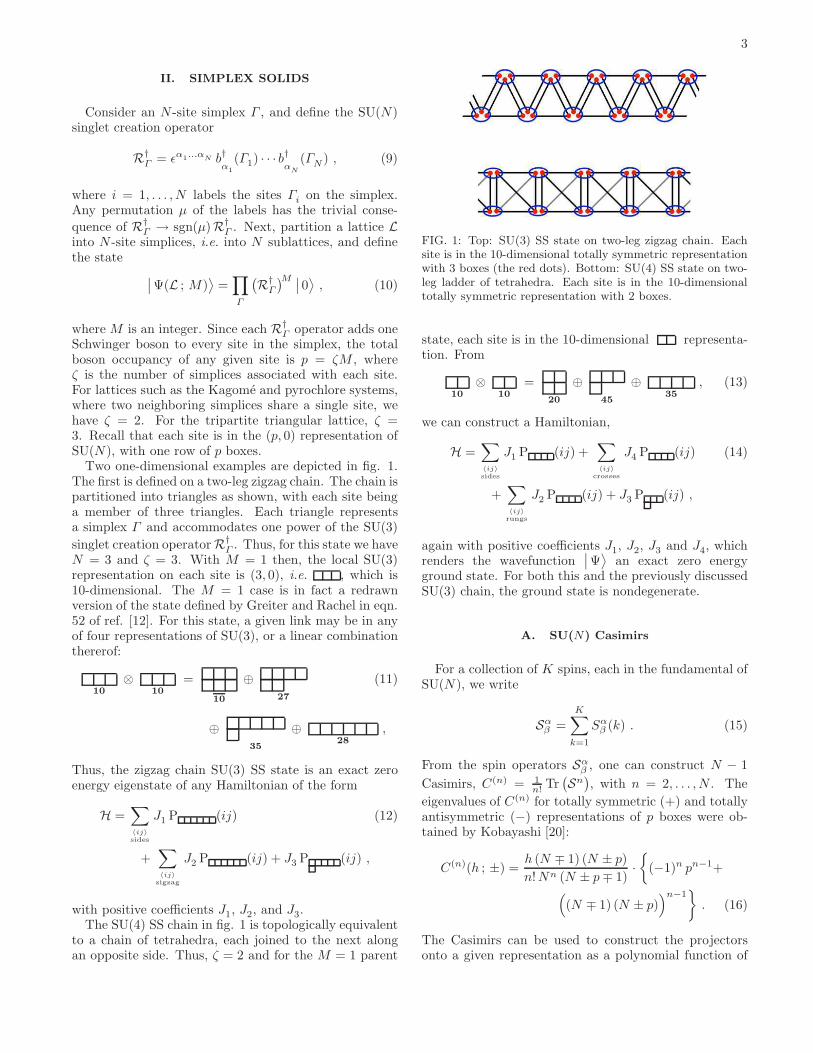
Two one-dimensional examples are depicted in fig. 1.The first is defined on a two-leg zigzag chain. The chain ispartitioned into triangles as shown, with each site beinga member of three triangles. Each triangle representsa simplex Γ and accommodates one power of the SU(3)

singlet creation operator R†Γ . Thus, for this state we have

N = 3 and ζ = 3. With M = 1 then, the local SU(3)representation on each site is (3, 0), i.e. , which is10-dimensional. The M = 1 case is in fact a redrawnversion of the state defined by Greiter and Rachel in eqn.52 of ref. [12]. For this state, a given link may be in anyof four representations of SU(3), or a linear combinationthererof:

10

⊗10

=

10

⊕27

(11)

⊕35

⊕28

,

Thus, the zigzag chain SU(3) SS state is an exact zeroenergy eigenstate of any Hamiltonian of the form

H =∑

〈ij〉sides

J1 P (ij) (12)

+∑

〈ij〉zigzag

J2 P (ij) + J3 P (ij) ,

with positive coefficients J1, J2, and J3.The SU(4) SS chain in fig. 1 is topologically equivalent

to a chain of tetrahedra, each joined to the next alongan opposite side. Thus, ζ = 2 and for the M = 1 parent

FIG. 1: Top: SU(3) SS state on two-leg zigzag chain. Eachsite is in the 10-dimensional totally symmetric representationwith 3 boxes (the red dots). Bottom: SU(4) SS state on two-leg ladder of tetrahedra. Each site is in the 10-dimensionaltotally symmetric representation with 2 boxes.

state, each site is in the 10-dimensional representa-tion. From

10

⊗10

=20

⊕45

⊕35

, (13)

we can construct a Hamiltonian,

H =∑

〈ij〉sides

J1 P (ij) +∑

〈ij〉crosses

J4 P (ij) (14)

+∑

〈ij〉rungs

J2 P (ij) + J3 P (ij) ,

again with positive coefficients J1, J2, J3 and J4, whichrenders the wavefunction

∣

∣Ψ⟩

an exact zero energyground state. For both this and the previously discussedSU(3) chain, the ground state is nondegenerate.

A. SU(N) Casimirs

For a collection of K spins, each in the fundamental ofSU(N), we write

Sαβ =

K∑

k=1

Sαβ (k) . (15)

From the spin operators Sαβ , one can construct N − 1

Casimirs, C(n) = 1n! Tr

(

Sn)

, with n = 2, . . . , N . The

eigenvalues of C(n) for totally symmetric (+) and totallyantisymmetric (−) representations of p boxes were ob-tained by Kobayashi [20]:

C(n)(h ; ±) =h (N ∓ 1) (N ± p)

n!Nn (N ± p∓ 1)·{

(−1)n pn−1+

(

(N ∓ 1) (N ± p))n−1

}

. (16)

The Casimirs can be used to construct the projectorsonto a given representation as a polynomial function of

4

the spin operators. In order to do so, though, we will needthe eigenvalues for all the representations which occur ina given product. Consider, for example, the case of threeSU(3) objects, each in their fundamental representation.We then have

3

⊗3

⊗3

= •1

⊕ 2 ·8

⊕10

. (17)

The eigenvalues of the quadratic and cubic Casimirs arefound to be

C(2)(•) = 0 C(2)( )

= 3 C(2)( ) = 6

C(3)(•) = −4 C(3)( )

= 0 C(3)( ) = 8 .

Therefore

P•(ijk) = 2 − 23 C

(2) + 14 C

(3) (18)

P (ijk) = −2 + C(2) − 12 C

(3) (19)

P (ijk) = 1 − 13 C

(2) + 14 C

(3) . (20)

Expressing the projector P (ijk) in terms of the localspin operators Sα

β (l), I find

P (ijk) = 1 − 16 Tr (S2

ijk) + 124 Tr (S3

ijk) (21)

= − 13 Tr

[

S(i)S(j) + S(j)S(k) + S(k)S(i)]

+ 18 Tr

[

S(i)S(j)S(k) + S(k)S(j)S(i)]

− 227 .

The projector thus contains both bilinear and trilinearterms in the local spin operators. One could also writethe projector in terms of the quadratic Casimir C(2) only,as

P (ijk) = 118 C

(2)(

C(2) − 3)

. (22)

This, however, would result in interaction terms suchas Tr

[

S(i)S(j)]

· Tr[

S(j)S(k)]

, which is apparentlyquadratic in S(j). For the representation, however,products such as Sα

β (i)Sµν (i) can be reduced to linear

combinations of the spin operators Sστ (i), as is familiar

in the case of SU(2). This simplification would then re-cover the expression in eqn. 21.

III. SS STATES IN d ≥ 2 DIMENSIONS

A. Kagome Lattice

The Kagome lattice, depicted in fig. 2, is a two-dimensional network of corner-sharing triangles, withζ = 2. It naturally accommodates a set of N = 3 SSstates. The simplest example consists of SU(3) objectsin the fundamental representation at each site, and places

FIG. 2: SU(3) simplex solid states on the Kagome lattice.

Applying the singlet operator R†Γ to all the up (down) tri-

angles generates the state˛

˛Ψ△

`

▽

´

¸

. Applying R†Γ to all the

triangular simplices generates the state˛

˛ Ψ¸

of eqn. 25. Thetwofold coordinated yellow sites at the top form a (10) edge(see sec. VIII).

SU(3) singlets on all the upward-pointing triangles (seefig. 2):

∣

∣Ψ△⟩

=∏

△R†

△∣

∣ 0⟩

. (23)

The lattice inversion operator I then generates a degen-

erate mate,∣

∣Ψ▽⟩

= I∣

∣Ψ△⟩

Both states are exact zeroenergy eigenstates of the Hamiltonian

H =∑

〈ijk〉∈120◦

P (ijk) , (24)

where the sum is over all 120◦ trios (ijk); there are sixsuch (ijk) trios for every hexagon. Since two of the threesites in each trio are antisymmetrized, The fully symmet-ric representation is completely absent. This modelbears obvious similarities to the MG model: its groundstate is a product over independent local singlets, hencethere are no correlations beyond a single simplex, and itspontaneously breaks a discrete lattice symmetry (in thiscase I) [21].

If we let the singlet creation operators act on both theup- and down-pointing triangles, we obtain a state whichbreaks no discrete lattice symmetries,

∣

∣Ψ⟩

=∏

△R†

△∏

▽R†

▽∣

∣ 0⟩

. (25)

For this state, each site is in the 6-dimensional rep-resentation. On any given link, then, there are the fol-lowing possibilities:

6

⊗6

=

6

⊕15

⊕15

. (26)

The fact that each link belongs to either an △ or ▽simplex, and the fact that a singlet operator R†

△/▽ is

5

associated with each simplex, means that no link can bein the fully symmetric representation. Thus,

∣

∣Ψ⟩

isan exact, zero-energy eigenstate of the Hamiltonian

H =∑

〈ij〉P (ij) . (27)

The states∣

∣Ψ△⟩

,∣

∣Ψ▽⟩

, and∣

∣Ψ⟩

are depicted in fig. 2.The actions of the quadratic and cubic Casimirs on the

possible representations for a given link are given in thefollowing table:

Repn C(2) C(3)

10/3 −80/27

16/3 64/27

28/3 352/27

Note that

C(3) = 83

(

C(2) − 32027

)

, (28)

hence the two Casimirs are not independent here. Wecan, however, write the desired projector,

P (ij) = 124

(

C(2) − 103

)(

C(2) − 163

)

(29)

= 124

(

Tr[

S(i)S(j)]

)2

+ 736 Tr

[

S(i)S(j)]

+ 527 ,

as a bilinear plus biquadratic interaction between neigh-boring spins. To derive this result, we write C(2) =12Tr

[

S(i) + S(j)]2

, whence

C(2) = Tr[

S(i)S(j)]

+ Tr(

S2)

= Tr[

S(i)S(j)]

+ p (N + p− 1) − p2

N. (30)

Next, consider the pyrochlore lattice in fig. 3. Thislattice consists of corner-sharing tetrahedra, with ζ = 2,and naturally accommodates an N = 4 SS state of theform

∣

∣Ψ⟩

=∏

tetrahedra

R†Γ

∣

∣ 0⟩

. (31)

Like the uniform SU(3) SS state on the Kagome lattice,this SU(4) state describes a lattice of spins which are inthe representation on each site; in the SU(4) casethis representation is 10-dimensional. From eqn. 13 wesee that each link, the sites of which appear in some sim-plex singlet creation operator, cannot have any weight

FIG. 3: The pyrochlore lattice and its quadripartite structure.

in the 35-dimensional totally symmetric repre-sentation. Hence, once again, the desired Hamiltonian isthat of eqn. 27. For SU(4),

C(2)( )

= 6 , C(2)( )

= 8 , C(2)( )

= 12 ,

and so

P (ij) = 124

(

C(2) − 6)(

C(2) − 8)

(32)

= 124

(

Tr[

S(i)S(j)]

)2

+ 16 Tr

[

S(i)S(j)]

+ 18 ,

Indeed, there is a rather direct correspondence betweenthe possible SU(3) SS states on the Kagome lattice andthe SU(4) SS states on the pyrochlore lattice. For exam-ple, one can construct a model with a doubly degenerateground state, similar to the MG model, by associating

the simplex singlet operators R†Γ with only the tetrahe-

dra which point along the (111) lattice direction.Finally, consider SU(4) states on the square lattice,

again in the representation on each site. We can once

again identify the exact ground state of the P (ij)Hamiltonian of eqn. 27. In this case, the ground stateis doubly degenerate, and is described by the ‘planar py-rochlore’ configuration shown in fig. 4.

IV. MAPPING TO A CLASSICAL MODEL

The correlations in the SS states are calculable usingthe coherent state representation. From results derivedin the Appendix I, the coherent state SS wavefunction isgiven by

Ψ[

{z(i)}]

= C∏

Γ

[

RΓ

(

z(Γ1) , . . . , z(ΓN ))

]M

, (33)

where C is a normalization constant, and

RΓ ≡ z(Γ1) ∧ z(Γ2) ∧ · · · ∧ z(ΓN )

= ǫα1...αN zα1

(Γ1) · · · zαN

(ΓN ) . (34)

6

FIG. 4: One of two doubly degenerate ground states forthe Hamiltonian of eqn. 27 applied to the square lattice,where each site is in the (2, 0, 0) representation of SU(4).The squares with crosses (or, equivalently, tetrahedra) repre-

sent singlet operators ǫαβγδ b†α(i) b†β(j) b†γ(k) b†δ(l) on the sim-

plex (ijkl). The resulting ‘planar pyrochlore’ configuration isequivalent to a checkerboard lattice of tetrahedra.

Here I have labeled the N sites on each simplex Γ by anindex i running from 1 to N .

Note that the coherent state probability density is

∣

∣Ψ∣

∣

2= |C|2

∏

Γ

∣

∣RΓ

∣

∣

2M, (35)

and that

∣

∣RΓ

∣

∣

2= ǫα1···αN ǫβ1···βN Q

α1β1

(Γ1) · · ·QαN

βN

(ΓN ) (36)

where Qαβ(i) = zα(i) zβ(i). Writing |Ψ|2 ≡ e−Hcl/T , wesee that that the probability density may be written asthe classical Boltzmann weight for a system described bythe classical Hamiltonian

Hcl = −∑

Γ

ln∣

∣RΓ

∣

∣

2, (37)

at a temperature T = 1/M [8, 22]. The classical inter-actions are N -body interaction, involving the matrices

Qαβ(i) on all the sites of a given N -site simplex, summedover all distinct simplices. For N = 2, this results in aclassical nearest-neighbor quantum antiferromagnet [8],with

HAKLT

cl = −∑

〈ij〉ln

(

1 − ni · nj

2

)

, (38)

with n = z†σz, where σ is the vector of Pauli matrices.This general feature of pair product wavefunctions of theBijl-Feynman, Laughlin, and AKLT form is thus valid forthe SS states as well.

As shown in Appendix I, the matrix element⟨

φ∣

∣ TK

∣

∣ψ⟩

of an operator

TK =∑

m,n

′T

k,lb1k1 · · · bN

kN b†1

l1 · · · b†NlN (39)

may be computed as an integral with respect to the mea-sure dµ (on each site) of the product φ(z)ψ(z) of coherentstate wavefunctions multiplied by the kernel

TK

(

{bα}, {b†α})

→(

N − 1 + p+K)

!

p !TK

(

{zα}, {zα})

.

(40)Thus, the quantum mechanical expectation values of Her-mitian observables in the SS states are expressible asthermal averages over the corresponding classical Hamil-

tonian Hcl of eqn. 37. The SS and VBS states thusshare the special property that their equal time quan-tum correlations are equivalent to thermal correlationsof an associated classical model on the same lattice, i.e.

in the same number of dimensions.

In this paper I will be content to merely elucidatethe correspondence between quantum correlations in∣

∣Ψ(L ; M⟩

) and classical correlations in Hcl. An applica-tion of this correspondence to a Monte Carlo evaluationof the classical correlations will be deferred to a futurepublication.

V. SINGLE MODE APPROXIMATION FORADJOINT EXCITATIONS

Following the treatment in ref. [8], I construct trialexcited states at wavevector k in the following manner.First, define the operator

φαβ(k) =∑

i

ηi φi,αβ(k) (41)

φi,αβ(k) = N−1/2∑

R

eik·R Sαβ (R, i) , (42)

where R is a Bravais lattice site and i labels the basiselements. Here, ηi is for the moment an arbitrary set ofcomplex-valued parameters and N is the total number of

unit cells in the lattice. The operators φαβ(k) transform

according to the (N2 − 1)-dimensional adjoint represen-tation of SU(N). Next, construct the trial state,

∣

∣φ⟩

≡ φαβ(k)∣

∣Ψ⟩

. (43)

and evaluate the expectation value of the Hamiltonian inthis state:

ESMA(k) =

⟨

φ∣

∣H∣

∣φ⟩

⟨

φ∣

∣φ⟩ =

η∗i fij(k) ηj

η∗i sij(k) ηj

. (44)

7

Here, fij(k) and sij(k) are, respectively, the oscillatorstrength and structure factor, given by

fij(k) = 12

⟨

Ψ∣

∣

[

φ†i,αβ(k) ,[

H , φj,αβ(k)]

]

∣

∣Ψ⟩

(45)

sij(k) =⟨

Ψ∣

∣φ†i,αβ(k)φj,αβ(k)∣

∣Ψ⟩

. (46)

Here I have assumed that H is a sum of local projec-

tors, and that H∣

∣Ψ⟩

= 0. Treating the ηi parametersvariationally, one obtains the equation

fij(k) ηj = ESMA

(k) sij(k) ηj . (47)

The lowest eigenvalue of this equation provides a rigorousupper bound to the lowest excitation energy at wavevec-tor k. The result is exact if all the oscillator strengthis saturated by a single mode, whence the SMA label.When

∣

∣Ψ⟩

is quantum-disordered, the SMA spectrum is

gapped. When∣

∣Ψ⟩

develops long-ranged order (for suf-ficiently large M parameter, and in d > 2 dimensions),the SMA spectrum is gapless.

VI. MEAN FIELD TREATMENT OFQUANTUM PHASE TRANSITION

The classical Hamiltonian of eqn 37 exhibits a global

SU(N) symmetry, where zσ(i) → Uσσ′ zσ′(i) for everylattice site i. Since the interactions are short-ranged,there can be no spontaneous breaking of this symmetryin dimensions d ≤ 2. In higher dimensions, the classicalmodel can order at finite temperature, corresponding toa quantum ordering at a finite value of m. For the AKLTstates, where N = 2, this phase transition was first dis-cussed in ref. [8]. I first discuss the N = 2 case and thengeneralize to arbitrary N > 2.

A. N = 2 : VBS States

Consider the N = 2 case, which on a lattice of coor-dination number z yields a family of wavefunctions de-scribing S = 1

2Mz objects with antiferromagnetic corre-lations. These are the AKLT valence bond solid (VBS)states. We have

z =

cos(

θ2

)

sin(

θ2

)

eiφ

, Q =1

2

1 + nz n+

n− 1 − nz

,

(48)where n = z†σz is a real unit vector, (σ are the Paulimatrices). Since

ǫα1β1 ǫα2β2 Qα1β1

(ΓA)Q

α2β2

(ΓB) = 1

2

(

1− nA· n

B

)

, (49)

the effective Hamiltonian is

Hcl = −∑

〈ij〉ln

(

1 − ni · nj

2

)

. (50)

The sum is over all links on the lattice. I assume thelattice is bipartite, so each link connects sites on the Aand B sublattices. I now make the mean field Ansatz

nA = m + δnA , nB = −m + δnB (51)

and expand H in powers of δni. Expanding to lowest

nontrivial order in the fluctuations δni, we obtain a meanfield Hamiltonian

HMF = E0 − hA

∑

i∈A

ni − hB

∑

j∈B

nj , (52)

where E0 is a constant and

hA

= −hB

=zm

1 + m2(53)

is the mean field. Here z is the lattice coordination num-ber. The self-consistency equation is then

m = 〈nA〉 =

∫

dn n ehA·n/T

/

∫

dn ehA·n/T , (54)

which yields

m = ctnhλ− 1

λ; λ =

z

T

m

1 +m2. (55)

The classical transition occurs at TMFc = 1

3z, so the SSstate exhibits a quantum phase transition at MMF

c =3z−1. For M > Mc the SS exhibits long-ranged two-sublattice Neel order. On the cubic lattice, the meanfield value MMF

c = 12 suggests that all the square lattice

VBS states, for which the minimal spin is S = 3 (withM = 1), are Neel ordered. Since the mean field treat-ment overestimates Tc due to its neglect of fluctuations,I conclude that the true Mc is somewhat greater than3z−1, which leaves open the possibility that the minimalM = 1 VBS state on the cubic lattice is a quantum dis-ordered state. Whether this is in fact the case could beaddressed by a classical Monte Carlo simulation.

B. N > 2 : SS States

For general N , I write

Qαβ(i) = 〈Qαβ(i) 〉 + δQαβ(i) , (56)

where the average is taken with respect to |Ψ|2 =

e−Hcl/T . To maximize |Ψ|2, i.e. to minimize Hcl, choose

a set{

Pσαβ

}

of N mutually orthogonal projectors, withσ = 1, . . . , N . The projectors satisfy the relations

Pσ Pσ′

= δσσ′ Pσ , (57)

and can each be written as

Pσαβ = ωσ

α ωσβ , (58)

8

where{

ωσ}

is a set of N mutually orthogonal CPN−1

vectors. Then if z(Γσ) = ωσ for each site Γσ in the

simplex, we haveRΓ = eiη, where η is an arbitrary phase,

and |RΓ |2 = 1. One then writes

Qσαβ ≡ 〈Qαβ(Γσ) 〉 =

1

Nδαβ +m

(

Pσαβ − 1

Nδαβ

)

. (59)

Here m ∈ [0, 1] is the order parameter, analogous to themagnetization. When m = 0, no special subspace is se-lected, and the correlations are isotropic. When m = 1,the Q-matrix is a projector onto the one-dimensional sub-space defined by ωσ. Note that 〈TrQ(Γσ) 〉 = 1, as itmust be.

At this point, there remains a freedom in assigning thevectors {ωσ} to the sites {Γσ} of each simplex. Consider,for example, the N = 3 case on the Kagome or triangu-lar lattice. The lattice is tripartite, so every A sublatticesite has 2 (Kagome) or 3 (triangular) nearest neighborson each of the B and C sublattices. However, as is well-known, the individual sublattices may have lower transla-tional symmetry than the underlying triangular Bravaislattice. Indeed, the sublattices may be translationallydisordered. I shall return to this point below. For themoment it is convenient to think in terms of N sublat-tices each of which has the same discrete symmetries asthe underlying Bravais lattice.

Expanding Hcl to lowest order in the fluctuations

δQαβ(i) on each site, and dropping terms of order (δQ)2

and higher, I obtain the mean field Hamiltonian,

HMF = E0 − ζ∑

i

hαβ(i)Qαβ(i) , (60)

where E0 is a constant. The mean field hαβ(i) is site-

dependent. On a ΓN site, we have

h(N)

αN

βN

=ǫα1α2...α

N ǫβ1β2...βN Q(1)

α1β1

· · ·Q(N−1)

αN−1β

N−1

ǫµ1...µN ǫν1...ν

N Q(1)

µ1ν1

· · · Q(N)

µN

νN

,

(61)In Appendix II I show that

hσαβ =

(

AN (m) δαβ +BN (m) Pσβα

)/

RN (m) , (62)

where

AN (m) = (N − 2) !

N−2∑

j=0

N − j − 1

j !mj

(

1 −m

N

)N−j−1

(63)

BN (m) = (N − 2) !

N−2∑

j=0

mj+1

j !

(

1 −m

N

)N−j−2

(64)

RN (m) = N !N∑

j=0

mj

j!

(

1 −m

N

)N−j

. (65)

Note that BN (0) = 0, BN (1) = 1, and R(1) = 1.The mean field Hamiltonian is then

HMF

= −∑

i

Tr(

ht(i)Q(i))

= −ζ BN (m)∑

i

∣

∣ω†(i) z(i)∣

∣

2, (66)

where hαβ(i) = hσ(i)αβ , where σ(i) labels the projector

associated with site i. The self-consistency relation is

obtained by evaluating the thermal average of Qαβ(i).

With xα ≡ |zα|2, I obtain

1

N+N − 1

Nm =

1∫

0

dx x (1 − x)N−2 exp(ζ bN(m)x/T )

1∫

0

dx (1 − x)N−2 exp(ζ bN (m)x/T )

,

(67)

where bN (m) = BN (m)/RN (m). It is simple to see thatm = 0 is a solution to this mean field equation. To findthe critical temperature Tc, expand the right hand sidein powers of m for small m. To lowest order, one finds

bN (m) =N

N − 1m+ O(m2) . (68)

The value of TMFc is determined by equating the coeffi-

cients of m on either side of the equation. I find

MMF

c (N, ζ) =1

TMFc (N, ζ)

=N2 − 1

ζ. (69)

This agrees with our previous result MMFc = 1

2 for theN = 2 state on the cubic lattice, for which ζ = 6. TheN = 3 SS on the Kagome lattice cannot develop long-ranged order which spontaneously breaks SU(N), owingto the Mermin-Wagner theorem. For the N = 4 SS onthe pyrochlore lattice, our mean field theory analysis sug-gests that the SS states are quantum disordered up toM ≈ 15

2 . Note that expression for MMFc reflects a compe-

tition between fluctuation effects, which favor disorder,and the coordination number, which favors order. Thenumerator, N2−1, is essentially the number of directionsin which Q can fluctuate about its average Q; this is thedimension of the Lie algebra su(N).

VII. ORDER BY DISORDER

At zero temperature, the classical model of eqn. 37 is

solved by maximizing∣

∣RΓ

∣

∣

2for each simplex Γ . This is

accomplished by partitioning the lattice L into N sublat-tices, such that no neighboring sites are elements of thesame sublattice. One then chooses any set of N mutually

orthogonal vectors ωσ ∈ CPN−1, and set zi = ωσ(i). On

every N -site simplex, then, each of the ωσ vectors will

9

FIG. 5: The Q = 0 structure on the Kagome lattice.

occur exactly once, resulting in∣

∣RΓ

∣

∣

2= 1, which is the

largest possible value. Thus, the model is unfrustrated,in the sense that every simplex Γ is fully satisfied by the

zi assignments, and the energy is the minimum possible

value: E0 = 0.For N = 2, there are two equivalent ways of partition-

ing a bipartite lattice into two sublattices. For N > 2,there are in general an infinite number of inequivalentpartitions, all of which have the same ground state en-

ergy E0 = 0. At finite temperature, though, the free en-ergy of these different orderings will in general differ, dueto the differences in their respective excitation spectra.A particular partition may then be selected by entropiceffects. This phenomenon is known as ‘order by disorder’[23, 24, 25].

To see how entropic effects might select a particularpartitioning, I derive a nonlinear σ-model, by expanding

Hcl about a particular zero-temperature ordered state.Start with

z(i) = ωσ(i)

(

1 − π†i πi

)1/2+ πi , (70)

where π†i ωσ(i) = 0. We may now expand

|RΓ |2 =∣

∣ǫα1···αN zα1(Γ1) · · · zα

N

(ΓN )∣

∣

2

= 1 − 12

∑

i,j

∣

∣ π†i ωσ(j) + ω†

σ(i) πj

∣

∣

2+ . . . (71)

Thus, the ‘low temperature’ classical Hamiltonian is

HLT =∑

〈ij〉

∣

∣ π†i ωσ(j) + ω†

σ(i) πj

∣

∣

2+ . . . , (72)

where the sum is over all nearest neighbor pairs on thelattice. The full SU(N) symmetry of the model is ofcourse not apparent in eqn. 72, since it is realized non-

linearly on the πi vectors.

Each πi vector is subject to a nonholonomic constraint,

π†i πi ≤ 1. To solve for the thermodynamics of HLT, I will

adopt a simplifying approximation, in which there is just

one nonholonomic constraint,∑

i π†i πi ≤ N , where N is

FIG. 6: The√

3 ×√

3 structure on the Kagome lattice.

the number of sites in the lattice. I fix the constraint byintroducing an auxiliary variable χ and demanding

N |χ|2 +∑

i

π†i πi = N , (73)

which I enforce with a Lagrange multiplier λ. The re-sulting model is

HLT =∑

〈ij〉

∣

∣ π†i ωσ(j)+ω

†σ(i) πj

∣

∣

2+λ(

N |χ|2+∑

i

π†i πi−N

)

.

(74)

The local constraints π†i ωσ(i) = 0 are retained.

It is convenient to rotate to a basis where ωσα = δα,σ,

in which case ω†σ(i) πj = πj,σ(i), i.e. the σ(i) component

of the vector πi. So long as σ(i) 6= σ(j) for nearest neigh-bors i and j, the local constraints have no effect on theHamiltonian. We are then left with a Gaussian theory in

the πi vectors. Leaving the constraint term aside for themoment, we can solve for the spectrum of the first part

of HLT. From this spectrum, we compute the density ofstates per site, g(ε). The free energy per site is then

F

N = −λ+ λ |χ|2 + T

∞∫

0

dε g(ε) ln

(

ε+ λ

T

)

. (75)

Since N is thermodynamically large, we can extremizewith respect to λ, to find the saddle point, yielding

1 = |χ|2 + T

∞∫

0

dεg(ε)

ε+ λ. (76)

Setting λ = χ = 0, I obtain an equation for Tc,

Tc =

[ ∞∫

0

dεg(ε)

ε

]−1

. (77)

For T < Tc, there is Bose condensation, and |χ|2 > 0.For T > Tc, the system is disordered. I stress that the

10

FIG. 7: Free energy for SU(3) simplex solid states on theKagome lattice. Dashed (red): Q = 0 structure. Solid (blue):√

3 ×√

3 structure.

disordered phase, described in this way, does not reflectthe SU(N) symmetry which must be present, owing tothe truncation in eqn. 72.

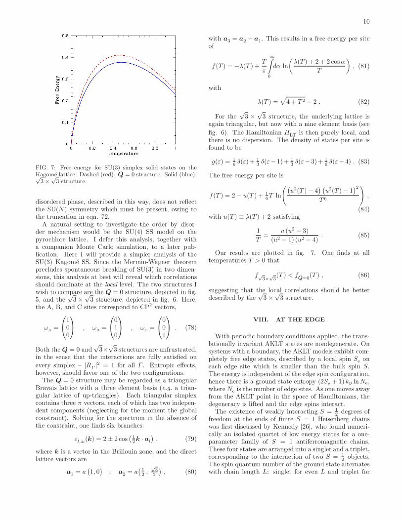
A natural setting to investigate the order by disor-der mechanism would be the SU(4) SS model on thepyrochlore lattice. I defer this analysis, together witha companion Monte Carlo simulation, to a later pub-lication. Here I will provide a simpler analysis of theSU(3) Kagome SS. Since the Mermin-Wagner theoremprecludes spontaneous breaking of SU(3) in two dimen-sions, this analysis at best will reveal which correlationsshould dominate at the local level. The two structures Iwish to compare are the Q = 0 structure, depicted in fig.5, and the

√3 ×

√3 structure, depicted in fig. 6. Here,

the A, B, and C sites correspond to CP2 vectors,

ωA =

100

, ωB =

010

, ωC =

001

. (78)

Both the Q = 0 and√

3×√

3 structures are unfrustrated,in the sense that the interactions are fully satisfied on

every simplex – |RΓ |2 = 1 for all Γ . Entropic effects,however, should favor one of the two configurations.

The Q = 0 structure may be regarded as a triangularBravais lattice with a three element basis (e.g. a trian-gular lattice of up-triangles). Each triangular simplexcontains three π vectors, each of which has two indepen-dent components (neglecting for the moment the globalconstraint). Solving for the spectrum in the absence ofthe constraint, one finds six branches:

εl,±(k) = 2 ± 2 cos(

12k · al

)

, (79)

where k is a vector in the Brillouin zone, and the directlattice vectors are

a1 = a(

1, 0)

, a2 = a(

12 ,

√3

2

)

, (80)

with a3 = a2 − a1. This results in a free energy per siteof

f(T ) = −λ(T ) +T

π

∞∫

0

dα ln

(

λ(T ) + 2 + 2 cosα

T

)

, (81)

with

λ(T ) =√

4 + T 2 − 2 . (82)

For the√

3 ×√

3 structure, the underlying lattice isagain triangular, but now with a nine element basis (see

fig. 6). The Hamiltonian HLT is then purely local, andthere is no dispersion. The density of states per site isfound to be

g(ε) = 16 δ(ε)+ 1

3 δ(ε− 1)+ 13 δ(ε− 3)+ 1

6 δ(ε− 4) . (83)

The free energy per site is

f(T ) = 2 − u(T ) + 16T ln

(

(

u2(T ) − 4) (

u2(T ) − 1)2

T 6

)

,

(84)with u(T ) ≡ λ(T ) + 2 satisfying

1

T=

u (u2 − 3)

(u2 − 1) (u2 − 4). (85)

Our results are plotted in fig. 7. One finds at alltemperatures T > 0 that

f√3×

√3(T ) < f

Q=0(T ) , (86)

suggesting that the local correlations should be betterdescribed by the

√3 ×

√3 structure.

VIII. AT THE EDGE

With periodic boundary conditions applied, the trans-lationally invariant AKLT states are nondegenerate. Onsystems with a boundary, the AKLT models exhibit com-pletely free edge states, described by a local spin Se oneach edge site which is smaller than the bulk spin S.The energy is independent of the edge spin configuration,hence there is a ground state entropy (2Se + 1) kB lnNe,where Ne is the number of edge sites. As one moves awayfrom the AKLT point in the space of Hamiltonians, thedegeneracy is lifted and the edge spins interact.

The existence of weakly interacting S = 12 degrees of

freedom at the ends of finite S = 1 Heisenberg chainswas first discussed by Kennedy [26], who found numeri-cally an isolated quartet of low energy states for a one-parameter family of S = 1 antiferromagnetic chains.These four states are arranged into a singlet and a triplet,corresponding to the interaction of two S = 1

2 objects.The spin quantum number of the ground state alternateswith chain length L: singlet for even L and triplet for

11

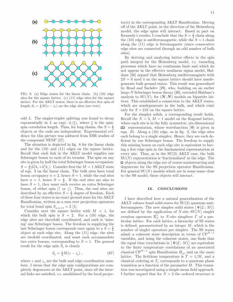
FIG. 8: (a) Edge states for the linear chain. (b) (10) edgesites for the square lattice. (c) (11) edge sites for the squarelattice. For the AKLT states, there is an effective free spin oflength Se = 1

2M(z − ze) on the edge sites (see text).

odd L. The singlet-triplet splitting was found to decayexponentially in L as exp(−L/ξ), where ξ is the spin-spin correlation length. Thus, for long chains, the S = 1

2objects at the ends are independent. Experimental evi-dence for this picture was adduced from ESR studies ofthe compound NENP [27].

The situation is depicted in fig. 8 for the linear chainand for the (10) and (11) edges on the square lattice.Recall that each link in the AKLT model supplies oneSchwinger boson to each of its termini. The spin on anysite is given by half the total Schwinger boson occupation:

S = 12 (b†↑b↑+b†↓b↓). Consider first the M = 1 AKLT state

of eqn. 3 on the linear chain. The bulk sites have totalboson occupancy n = 2, hence S = 1, while the end siteshave n = 1, hence S = 1

2 . If the end sites are also tohave S = 1, they must each receive an extra Schwingerboson, of either spin (↑ or ↓). Thus, the end sites aredescribed by an effective S = 1

2 degree of freedom. Eachof these four states is an exact ground state for the AKLTHamiltonian, written as a sum over projection operators

for total bond spin Sn,n+1 = 2 [1].Consider next the square lattice with M = 1, for

which the bulk spin is S = 2. For a (10) edge, theedge sites are threefold coordinated, and each is ‘miss-ing’ one Schwinger boson. The freedom in supplying thelast Schwinger boson corresponds once again to a S = 1

2object at each edge site. Along the (11) edge, the sitesare twofold coordinated, and must each accommodatetwo extra bosons, corresponding to S = 1. The generalresult for the edge spin Se is clearly

Se = 12M(z − ze) , (87)

where z and ze are the bulk and edge coordination num-bers. I stress that the edge spin configurations are com-pletely degenerate at the AKLT point, since all the inter-nal links are satisfied, i.e. annihilated by the local projec-

tor(s) in the corresponding AKLT Hamiltonian. Movingoff of the AKLT point, in the direction of the Heisenbergmodel, the edge spins will interact. Based in part onKennedy’s results, I conclude that the S = 1

2 chain alongthe (10) edge is antiferromagnetic, while the S = 1 chainalong the (11) edge is ferromagnetic (since consecutiveedge sites are connected through an odd number of bulksites).

By deriving and analyzing lattice effects in the spinpath integral for the Heisenberg model, i.e. tunnelingprocesses which have no continuum limit and which donot appear in the effective nonlinear sigma model, Hal-dane [28] argued that Heisenberg antiferromagnets with2S = 0 mod 4 on the square lattice should have nonde-generate bulk ground states. This result was generalizedby Read and Sachdev [29], who, building on an earlierlarge-N Schwinger boson theory [30], extended Haldane’sanalysis to SU(N), for (N , N ) models on bipartite lat-tices. This established a connection to the AKLT states,which are nondegenerate in the bulk, and which existonly for S = 2M on the square lattice.

For the simplex solids, a corresponding result holds.Recall the N = 3, M = 1 model on the Kagome lattice,where each site is in the fully symmetric, six-dimensional

representation, whose wavefunction∣

∣Ψ⟩

is given ineqn. 25. Along a (10) edge, as in fig. 2, the edge siteseach belong to a single simplex. Hence, they are each de-ficient by one Schwinger boson. The freedom to supplythis missing boson on each edge site is equivalent to hav-ing a free edge spin in the fundamental representation atevery site. Thus, as in the SU(2) AKLT case, the bulkSU(N) representation is ‘fractionalized’ at the edge. The

objects along the edge are of course noninteracting anddegenerate for the SS projection operator Hamiltonian.For general SU(N) models which are in some sense closeto the SS model, these objects will interact.

IX. CONCLUSIONS

I have described here a natural generalization of theAKLT valence bond solid states for SU(2) quantum anti-ferromagnets. The new simplex solid states

∣

∣Ψ(L ; M)⟩

are defined by the application of N -site SU(N) singlet

creation operators R†Γ to N -site simplices Γ of a par-

ticular lattice. For each lattice, a hierarchy of SS statesis defined, parameterized by an integer M , which is thenumber of singlet operators per simplex. The SS statesadmit a coherent state description in terms of CPN−1

variables, and using the coherent states, one finds thatthe equal time correlations in

∣

∣Ψ(L ; M)⟩

are equivalentto the finite temperature correlations of an associated

classical CPN−1 spin Hamiltonian Hcl, and on the samelattice. The fictitious temperature is T = 1/M , and aclassical ordering at Tc corresponds to a quantum phasetransition as a function of the parameter M . This transi-tion was investigated using a simple mean field approach.I further argued that for N > 2 the ordered structure is

12

selected by an ‘order by disorder’ mechanism, which inthe classical model amounts to an entropic favoring ofone among many degenerate T = 0 structures. I hope to

report on classical Monte Carlo study of Hcl on Kagome(N = 3) and pyrochlore (N = 4) lattices in a futurepublication; there the coherent state formalism derivedhere will be more extensively utilized. Finally, a kind of‘fractionalization’ of the bulk SU(N) representation atthe edge was discussed.

X. ACKNOWLEDGMENTS

This work grew out of conversations with Congjun Wu,to whom I am especially grateful for many several stim-ulating and useful discussions. I thank Shivaji Sondhi(who suggested the name “simplex solid”) for readingthe manuscript and for many insightful comments. I amindebted to Martin Greiter and Stephan Rachel for acritical reading of the manuscript, and for several helpfulsuggestions and corrections. I also gratefully acknowl-edge discussions with Eduardo Fradkin.

XI. APPENDIX I : PROPERTIES OF SU(N)COHERENT STATES

A. Definition of SU(N) coherent states

Consider the fully symmetric representation of SU(N)with p boxes in a single row I call this the p-representation, of dimension

(

N+p−1p

)

. Define the state

∣

∣ z ; p⟩

=1√p!

(

z1 b†1 + . . .+ zN b†N

)p ∣∣ 0⟩

, (88)

where z ∈ CPN−1 is a complex unit vector, with z†z = 1.In order to establish some useful properties regarding theSU(N) coherent states, it is convenient to consider theunnormalized coherent states

∣

∣ z , ξ)

= exp(

ξ zµ b†µ

) ∣

∣ 0⟩

=

∞∑

p=0

ξp

√p!

∣

∣ z ; p⟩

. (89)

Clearly∣

∣ z , ξ)

is a product ofN (unnormalized) coherentstates for the N Schwinger bosons. One then has

(

z , ξ∣

∣ z′ , ξ′)

= exp(

ξξ′ z†z′)

=

∞∑

p=0

(ξξ)p

p!

⟨

z ; p∣

∣ z′ ; p⟩

(90)

Equating the coefficients of (ξξ)p, one obtains the coher-ent state overlap,

⟨

z ; p∣

∣ z′ ; p⟩

=(

z†z′)p. (91)

B. Resolution of identity

Define the measure

dµ =

N∏

j=1

dRe(zj) d Im(zj)

πδ(

z†z − 1)

(92)

Next, consider the expression

P(ξ, ξ) =

∫

dµ∣

∣ z , ξ) (

z , ξ∣

∣

=∑

n1···nN

(

ξξ)

P

j nj

∏

j nj !INn1···nN

∣

∣n⟩ ⟨

n∣

∣

=∞∑

p=0

(

ξξ)p

p!

∫

dµ∣

∣ z ; p⟩ ⟨

z ; p∣

∣ (93)

where∣

∣n⟩

=∣

∣n1, . . . , nN

⟩

and

INn1···nN

≡1∫

0

dx1 · · ·1∫

0

dxN δ

( N∑

j=1

xj − 1

) N∏

j=1

xnj

j . (94)

Here, xj =∣

∣zj

∣

∣

2. If we define xj = (1 − xN ) yj for j =

1, . . . , N−1, then by integrating over xN one obtains theresult

INn1···nN

= IN−1

n1···nN−1

·1∫

0

dxN xn

N

N

(

1 − xN )N−2+PN−1

j=1 nj

=nN !

(

N − 2 +∑N−1

j=1 nj

)

!(

N − 1 +∑N−1

j=1 nj

)

!· IN−1

n1···nN−1

=n1! · · · nN !

(

N − 1 + n1 + . . .+ nN

)

!. (95)

Thus, equating the coefficient of(

ξξ)p

in eqn 93, onearrives at the result

11p =(N − 1 + p) !

p !

∫

dµ∣

∣ z ; p⟩⟨

z ; p∣

∣ , (96)

where the projector onto the p-representation is

11p ≡∑

n1···nN

δp,

P

j nj

∣

∣n⟩ ⟨

n∣

∣ . (97)

C. Continuous representation of a state˛

˛ψ¸

Let us define the state

∣

∣ψ⟩

≡ 1√p !ψ(

b†1, . . . , b†N

)∣

∣ 0⟩

=1√p !

∑

n

′ψn b

†1

n1 · · · b†Nn

N∣

∣ 0⟩

, (98)

13

where n = {n1, . . . , nN}, and where the prime on the

sum reflects the constraint∑N

j=1 nj = p. The overlap of∣

∣ψ⟩

with the coherent state∣

∣ z ; p⟩

is

⟨

z ; p∣

∣ψ⟩

=∑

n

′ψn z

n11 · · · zn

N

N (99)

= ψ(z1, . . . , zN ) . (100)

D. Matrix elements of representation-preservingoperators

Next, consider matrix elements of the generalrepresentation-preserving operator,

TK =∑

m,n

′T

k,lb1

k1 · · · bNk

N b†1l1 · · · b†N

lN . (101)

Here the prime on the sum indicates a constraint∑N

j=1 kj =∑N

j=1 lj = K. Then

⟨

φ∣

∣ TK

∣

∣ψ⟩

=1

p !

∑

m,nk,l

′′T

k,lφ∗m ψn (102)

×N∏

j=1

[

(mj + kj

)

! δm

j+k

j,n

j+l

j

]

,

where the double prime on the sum indicates constraintson each of the sums for m, n, k, and l. This may alsobe computed as an integral over coherent state wavefunc-tions:

∫

dµ φ(z)TK(z, z)ψ(z) =∑

m,nk,l

φm Tk,lψn

×N∏

j=1

zm

j+k

j

j zn

j+l

j

j

=∑

m,nk,l

′′INm+k φm T

k,lψn

N∏

j=1

δm

j+k

j,nq+ln

=p !

(

N − 1 + p+K)

!

⟨

φ∣

∣ TK

∣

∣ψ⟩

. (103)

Thus, the general matrix element may be written

⟨

φ∣

∣ TK

∣

∣ψ⟩

=

(

N − 1 + p+K)

!

p !

∫

dµ φ(z)TK(z, z)ψ(z) ,

(104)

where TK(z, z) is obtained from eqn. 101 by substitution

bj → zj and b†j → zj .

XII. APPENDIX II : THE LOCAL MEAN FIELD

With the definition of eqn. 59, I first compute

RN (m) ≡ Q(1) ∧ · · · ∧ Q(N)

= ǫα1...αN ǫβ1...β

N

(1 −m

Nδα1β1

+mP1α1β1

)

· · ·(1 −m

Nδα

Nβ

N

+mPNα

Nβ

N

)

,

(105)

where

Pσαβ = ωσ

β ωσα (106)

is the projector onto subspace spanned by ωσ. I nowsystematically expand in powers of the projectors andcontract over all free indices. The result is

RN (m) = N !N∑

j=0

ml

j!

(

1 −m

N

)N−j

.

The local mean field on a j = 1 site is given by theexpression in eqn. 61. Expanding the numerator,

RN (m)hNα

Nβ

N

= ǫα1α2...αN ǫβ1β2...β

N Q(1)

α1β1

· · · Q(N−1)

αN−1β

N−1

,

(107)in powers of the projectors, the term of order j is

(N − j − 1)!

(

1 −m

N

)N−j−1

mj ǫα1α2...αN ǫβ1β2...β

N

×∑

k1<...<kj<N

Pk1

α1β1

Pk2

α2β2

· · ·PkN−1

αN−1β

N−1

(108)

Writing

ǫα1α2...αN ǫβ1β2...β

N =∑

σ∈SN

sgn(σ) δα1β

σ(1)

· · · δα

Nβ

σ(N)

,

(109)we see that once this is inserted into eqn. 108, the onlysurviving permutations are the identity, and the (N − 1)two-cycles which include index N . All other permuta-tions result in contractions of indices among orthogonalprojectors, and hence yield zero. Furthermore using com-pleteness, we have

N−1∑

i=1

Piβ

Nα

N

= δβ

Nα

N

− P(N

βN

αN

. (110)

14

Thus,

ǫα1α2...αN ǫβ1β2...β

N

∑

k1<...<kj<N

Pk1

α1β1

Pk2

α2β2

· · ·PkN−1

αN−1β

N−1

=

(

N − 1

j

)

δβ

Nα

N

−∑

k1<...<kj<N

j∑

l=1

Pk

l

βN

αN

=

=

(

N − 1

j

)

δβ

Nα

N

−(

N − 2

j − 1

)

(

δβ

Nα

N

− PNβ

Nα

N

)

=

(

N − 2

j

)

δβ

Nα

N

+

(

N − 2

j − 1

)

PNβ

Nα

N

. (111)

From this expression, I obtain the results of eqns. 62, 63,64, and 65.

[1] I. Affleck, T. Kennedy, E. H. Lieb, and H. Tasaki, Phys.

Rev. Lett. 59, 799 (1987); Comm. Math. Phys, 115, 477(1988).

[2] W. Marshall, Proc. Roy. Soc. A 232, 48 (1955).[3] E. Lieb and D. C. Mattis, J. Math. Phys. 3, 749 (1962).[4] P. W. Anderson, Mater. Res. Bull. 8, 153 (1973); Science

235, 1196 (1987); P. Fazekas and P. W. Anderson, Phil.

Mag. 30, 423 (1974).[5] S. Liang, B. Doucot, and P. W. Anderson, Phys. Rev.

Lett. 61, 365 (1988).[6] C. K. Majumdar and D. K. Ghosh, J. Math. Phys. 10,

1388 (1969); C. K. Majumdar, J. Phys. C 3, 911 (1970);P. M. can den Broek, Phys. Lett. A 77, 261 (1980).

[7] D. J. Klein, J. Phys. A 15, 661 (1982).[8] D. P. Arovas, A. Auerbach, and F. D. M. Haldane, Phys.

Rev. Lett. 60, 531 (1988).[9] I. Affleck, Phys. Rev. Lett. 54, 966 (1985).

[10] It is worth remarking that the AKLT states themselvesdo not require a bipartite lattice, and indeed can be de-fined on any lattice. The corresponding classical model,given in eqn. 38, is then frustrated.

[11] I. Affleck, D. P. Arovas, J. B. Marson, and D. A. Rabson,Nucl. Phys. B 366, 467 (1991).

[12] Martin Greiter and Stephan Rachel, Phys. Rev. B 75,184441 (2007).

[13] Shun-Qing Shen, Phys. Rev. B 64, 132411 (2001).[14] Zohar Nussinov and Gerardo Ortiz, preprint

arXiv:cond-mat/0702377, sections XIV and XV.[15] Shu Chen, Congjun Wu, Shou-Cheng Zhang, and Yupeng

Wang, Phys. Rev. B 72, 214428 (2005).[16] S. Pankov, R. Moessner, and S. L. Sondhi, preprint

arXiv:cond-mat/07050846.[17] D. S. Rokhsar and S. A. Kivelson, Phys. Rev. Lett. 61,

2376 (1988).[18] T. Senthil and M. P. A. Fisher, Phys. Rev. B 63, 134521

(2001).[19] G. Misguich, D. Serban, and V. Pasquier, Phys. Rev.

Lett. 89, 137202 (2002).[20] Kozo Kobayashi, Prog. Theor. Phys. 49, 345 (1973). I

have normalized the Casimirs C(n) by a factor of 1n!

.

[21] By taking linear combinations˛

˛ Ψ△

¸

±˛

˛ Ψ▽

¸

, one canconstruct I eigenstates with eigenvalues ±1. A similarstate of affairs holds for the MG model, where groundstates of well-defined crystal momentum k = 0 and k = π

may be constructed from the degenerate broken symme-try wavefunctions.

[22] R. B. Laughlin, Phys. Rev. Lett. 50, 1395 (1983).[23] J. Villain, R. Bidaux, J.-P. Carton, and R. Conte, J.

Phys. (France) 41, 1263 (1980).[24] E. F. Shender, Sov. Phys. JETP 56, 178 (1982).[25] C. L. Henley, Phys. Rev. Lett. 62, 2056 (1989).[26] Tom Kennedy, J. Phys. Cond. Mat. 2, 5737 (1990).[27] M. Hagiwara, K. Katsumata, I. Affleck, B. I. Halperin,

and J. P. Renard, Phys. Rev. Lett 65, 3181 (1990); S. H.Glarum, S. Geschwind, K M. Lee, M. L. Kaplan, and J.Michel, Phys. Rev. Lett. 67, 1614 (1991).

[28] F. D. M. Haldane, Phys. Rev. Lett. 61, 1029 (1988).[29] N. Read and Subir Sachdev, Phys. Rev. Lett. 62, 1694

(1989).[30] D. P. Arovas and A. Auerbach, Phys. Rev. B 38, 316

(1988).