Available online at www.sciencedirect.com

www.elsevier.com/locate/compfluid

Computers & Fluids 37 (2008) 907–930

Review

The MAC method

S. McKee a,*, M.F. Tome b, V.G. Ferreira b, J.A. Cuminato b,A. Castelo b, F.S. Sousa b, N. Mangiavacchi c

a Department of Mathematics, University of Strathclyde, Livingstone Tower, 26 Richmond Street, Glasgow G1 1XH, UKb Department of Applied Mathematics and Statistics, University of Sao Paulo, USP, Sao Carlos, SP, Brazilc Department of Mechanical Engineering, State University of Rio de Janeiro, UERJ, Rio de Janeiro, Brazil

Received 1 January 2007; accepted 4 October 2007Available online 24 November 2007

Abstract

In this article recent advances in the Marker and Cell (MAC) method will be reviewed. The MAC technique dates back to the early1960s at the Los Alamos Laboratories and this article starts with a historical review, and then a brief discussion of related techniques.Improvements since the early days of MAC (and the Simplified MAC – SMAC) include automatic time-stepping, the use of the conjugategradient method to solve the Poisson equation for the corrected velocity potential, greater efficiency through stripping out the virtualparticles (markers) other than those near the free surface, and more accurate approximations of the free surface boundary conditions,the addition of bounded high accuracy upwinding for the convected terms (thereby being able to solve higher Reynolds number flows),and a (dynamics) flow visualization facility. More recently, effective techniques for surface and interfacial flows and, in particular, foraccurately tracking the associated surface(s)/interface(s) including moving contact angles have been developed. This article will concen-trate principally on a three-dimensional version of the SMAC method. It will eschew both code verification and model validation; insteadit will emphasize the applications that the MAC method can solve, from multiphase flows to rheology.� 2007 Elsevier Ltd. All rights reserved.

Contents

1. Introduction . . . . . . . . . . . . . . . . . . . . . . . . . . . . . . . . . . . . . . . . . . . . . . . . . . . . . . . . . . . . . . . . . . . . . . . . . . . . . . 9082. Background of the marker and cell method . . . . . . . . . . . . . . . . . . . . . . . . . . . . . . . . . . . . . . . . . . . . . . . . . . . . . . . . 9083. A review of interfacial tracking techniques . . . . . . . . . . . . . . . . . . . . . . . . . . . . . . . . . . . . . . . . . . . . . . . . . . . . . . . . . 9104. The emphasis of the review . . . . . . . . . . . . . . . . . . . . . . . . . . . . . . . . . . . . . . . . . . . . . . . . . . . . . . . . . . . . . . . . . . . . 9115. Governing equations. . . . . . . . . . . . . . . . . . . . . . . . . . . . . . . . . . . . . . . . . . . . . . . . . . . . . . . . . . . . . . . . . . . . . . . . . 911

0045-79

doi:10.1

* CorrE-m

5.1. Boundary conditions . . . . . . . . . . . . . . . . . . . . . . . . . . . . . . . . . . . . . . . . . . . . . . . . . . . . . . . . . . . . . . . . . . . . 9125.2. Interfacial and free surface conditions . . . . . . . . . . . . . . . . . . . . . . . . . . . . . . . . . . . . . . . . . . . . . . . . . . . . . . . . 912

6. Discretization. . . . . . . . . . . . . . . . . . . . . . . . . . . . . . . . . . . . . . . . . . . . . . . . . . . . . . . . . . . . . . . . . . . . . . . . . . . . . . 912

6.1. Markers and cells . . . . . . . . . . . . . . . . . . . . . . . . . . . . . . . . . . . . . . . . . . . . . . . . . . . . . . . . . . . . . . . . . . . . . . 9146.2. Initial approximation of the free surface . . . . . . . . . . . . . . . . . . . . . . . . . . . . . . . . . . . . . . . . . . . . . . . . . . . . . . 9146.3. Interfacial tension effects . . . . . . . . . . . . . . . . . . . . . . . . . . . . . . . . . . . . . . . . . . . . . . . . . . . . . . . . . . . . . . . . . 9146.4. Surface merging and splitting . . . . . . . . . . . . . . . . . . . . . . . . . . . . . . . . . . . . . . . . . . . . . . . . . . . . . . . . . . . . . . 915

6.4.1. Merging . . . . . . . . . . . . . . . . . . . . . . . . . . . . . . . . . . . . . . . . . . . . . . . . . . . . . . . . . . . . . . . . . . . . . . . 9156.4.2. Demerging . . . . . . . . . . . . . . . . . . . . . . . . . . . . . . . . . . . . . . . . . . . . . . . . . . . . . . . . . . . . . . . . . . . . . 916

30/$ - see front matter � 2007 Elsevier Ltd. All rights reserved.

016/j.compfluid.2007.10.006

esponding author. Tel.: +44 0 141 548 3671; fax: +44 0 141 548 3345.ail address: smck@maths.strath.ac.uk (S. McKee).

908 S. McKee et al. / Computers & Fluids 37 (2008) 907–930

7. Numerical procedure . . . . . . . . . . . . . . . . . . . . . . . . . . . . . . . . . . . . . . . . . . . . . . . . . . . . . . . . . . . . . . . . . . . . . . . . 916

7.1. Time-stepping procedure . . . . . . . . . . . . . . . . . . . . . . . . . . . . . . . . . . . . . . . . . . . . . . . . . . . . . . . . . . . . . . . . . 9177.2. Finite difference approximation of the convective terms . . . . . . . . . . . . . . . . . . . . . . . . . . . . . . . . . . . . . . . . . . . 917

8. Undulation removal . . . . . . . . . . . . . . . . . . . . . . . . . . . . . . . . . . . . . . . . . . . . . . . . . . . . . . . . . . . . . . . . . . . . . . . . . 917

8.1. Normal vector calculation . . . . . . . . . . . . . . . . . . . . . . . . . . . . . . . . . . . . . . . . . . . . . . . . . . . . . . . . . . . . . . . . 9188.2. Vertex balance procedure . . . . . . . . . . . . . . . . . . . . . . . . . . . . . . . . . . . . . . . . . . . . . . . . . . . . . . . . . . . . . . . . . 9188.3. Undulation removal procedure . . . . . . . . . . . . . . . . . . . . . . . . . . . . . . . . . . . . . . . . . . . . . . . . . . . . . . . . . . . . . 919

9. Curvature calculation . . . . . . . . . . . . . . . . . . . . . . . . . . . . . . . . . . . . . . . . . . . . . . . . . . . . . . . . . . . . . . . . . . . . . . . . 919

9.1. Normal vector approximation . . . . . . . . . . . . . . . . . . . . . . . . . . . . . . . . . . . . . . . . . . . . . . . . . . . . . . . . . . . . . 9209.2. Curvature approximation. . . . . . . . . . . . . . . . . . . . . . . . . . . . . . . . . . . . . . . . . . . . . . . . . . . . . . . . . . . . . . . . . 920

10. A dynamic contact angle . . . . . . . . . . . . . . . . . . . . . . . . . . . . . . . . . . . . . . . . . . . . . . . . . . . . . . . . . . . . . . . . . . . . . 92011. Data structure and system environment . . . . . . . . . . . . . . . . . . . . . . . . . . . . . . . . . . . . . . . . . . . . . . . . . . . . . . . . . . . 921

11.1. Data structure . . . . . . . . . . . . . . . . . . . . . . . . . . . . . . . . . . . . . . . . . . . . . . . . . . . . . . . . . . . . . . . . . . . . . . . . 92111.2. The module Modflow-3D. . . . . . . . . . . . . . . . . . . . . . . . . . . . . . . . . . . . . . . . . . . . . . . . . . . . . . . . . . . . . . . . 92211.3. The module Simflow-3D . . . . . . . . . . . . . . . . . . . . . . . . . . . . . . . . . . . . . . . . . . . . . . . . . . . . . . . . . . . . . . . . 92211.4. The module Visflow-3D . . . . . . . . . . . . . . . . . . . . . . . . . . . . . . . . . . . . . . . . . . . . . . . . . . . . . . . . . . . . . . . . . 92311.5. Communication between the modules . . . . . . . . . . . . . . . . . . . . . . . . . . . . . . . . . . . . . . . . . . . . . . . . . . . . . . . 923

12. Applications . . . . . . . . . . . . . . . . . . . . . . . . . . . . . . . . . . . . . . . . . . . . . . . . . . . . . . . . . . . . . . . . . . . . . . . . . . . . . . 923

12.1. Jet buckling . . . . . . . . . . . . . . . . . . . . . . . . . . . . . . . . . . . . . . . . . . . . . . . . . . . . . . . . . . . . . . . . . . . . . . . . . 92312.2. Splashing drop . . . . . . . . . . . . . . . . . . . . . . . . . . . . . . . . . . . . . . . . . . . . . . . . . . . . . . . . . . . . . . . . . . . . . . . 92312.3. Hydraulic jump . . . . . . . . . . . . . . . . . . . . . . . . . . . . . . . . . . . . . . . . . . . . . . . . . . . . . . . . . . . . . . . . . . . . . . . 92412.4. Rising bubbles. . . . . . . . . . . . . . . . . . . . . . . . . . . . . . . . . . . . . . . . . . . . . . . . . . . . . . . . . . . . . . . . . . . . . . . . 92412.5. Container filling . . . . . . . . . . . . . . . . . . . . . . . . . . . . . . . . . . . . . . . . . . . . . . . . . . . . . . . . . . . . . . . . . . . . . . 925

13. Viscoelastic flows . . . . . . . . . . . . . . . . . . . . . . . . . . . . . . . . . . . . . . . . . . . . . . . . . . . . . . . . . . . . . . . . . . . . . . . . . . . 925

13.1. Oldroyd-B. . . . . . . . . . . . . . . . . . . . . . . . . . . . . . . . . . . . . . . . . . . . . . . . . . . . . . . . . . . . . . . . . . . . . . . . . . . 92513.2. Elastic jet . . . . . . . . . . . . . . . . . . . . . . . . . . . . . . . . . . . . . . . . . . . . . . . . . . . . . . . . . . . . . . . . . . . . . . . . . . . 92513.3. Die-Swell . . . . . . . . . . . . . . . . . . . . . . . . . . . . . . . . . . . . . . . . . . . . . . . . . . . . . . . . . . . . . . . . . . . . . . . . . . . 927

14. Future developments . . . . . . . . . . . . . . . . . . . . . . . . . . . . . . . . . . . . . . . . . . . . . . . . . . . . . . . . . . . . . . . . . . . . . . . . 927Acknowledgements . . . . . . . . . . . . . . . . . . . . . . . . . . . . . . . . . . . . . . . . . . . . . . . . . . . . . . . . . . . . . . . . . . . . . . . . . . 928References . . . . . . . . . . . . . . . . . . . . . . . . . . . . . . . . . . . . . . . . . . . . . . . . . . . . . . . . . . . . . . . . . . . . . . . . . . . . . . . . 928

1. Introduction

The purpose of this article is to provide an overview ofthe recent advances in the MAC method. Although it is atechnology dating back to the early sixties at the Los Ala-mos Laboratories, with the considerably greater computingpower that we now enjoy, it is witnessing a revival and, forfree surface fluid flow problems, showing itself the equal ofany of the competing methods.

This review article will provide a brief history of theMAC technique, and even briefer description of relatedmethods but will include a fairly complete descriptionof the techniques and ideas behind the method. It willshow that, with high order monotone upwinding approx-imation of the inertial terms, high Reynolds numberflows are attainable and this will be illustrated by a sim-ulation of the hydraulic jump. Viscous jet flow will bestudied, particularly viscous jet buckling, examples ofcontainer filling will be given, and a liquid drop splash-ing onto a quiescent fluid will be simulated. Finally, weshall show how to extend the MAC method to viscoelas-tic fluid flow, thus opening up the field of computationalfree surface rheology, to which the method is particularlywell adapted.

2. Background of the marker and cell method

There was a prolific development of computationalfluid dynamics (CFD) methods in the fluid dynamicsgroup at Los Alamos Laboratories in the years from1958 to the late 1960s. This development was largelydue to the energy, creativity and leadership of FrancisHarlow. It was he who in 1958 developed the originalparticle-in-cell (PIC) code [21,35], which used mass parti-cles that carried material position, mass and speciesinformation. Despite the special capabilities of PIC forfollowing discontinuities, it did not give accurate solu-tions in general because the transfer of informationbetween the particles and the underlying grid resultedin numerical diffusion. Twenty years ago, in the 1980s,there was a resurgence of interest in particle methods,resulting in a variant called FLIP (e.g. see [7,8]); FLIPovercame this difficulty of numerical diffusion to a largeextent. The principal applications of FLIP have been inmagnetohydrodynamic flows, in the earth’s magneto-sphere and the sun’s heliosphere (see e.g. [9]).

The MAC method first appeared in 1965. It was devel-oped by Harlow and Welch [36,104] specifically for freesurface flows as a variant of PIC method. Based on an

S. McKee et al. / Computers & Fluids 37 (2008) 907–930 909

Eulerian staggered grid system, the MAC method is a finitedifference solution technique for investigating the dynamicsof an incompressible viscous fluid. It employs the primitivevariables of pressure and velocity. One of the key featuresis the use of Lagrangian virtual particles, whose coordi-nates are stored, and which move from a cell to the nextaccording to the latest computed velocity field. If a cell con-tains a particle it is deemed to contain fluid, thus providingflow visualization of the free surface. In 1970, Amsden andHarlow [1] subsequently developed a simplified MACmethod (SMAC) which circumvented difficulties with theoriginal method by splitting the calculation cycle into twoparts, namely: a provisional velocity field calculation fol-lowed by a velocity revision employing an auxiliary poten-tial function to ensure incompressibility throughout. In thisreport, Amsden and Harlow describe a specific program,ZUNI, which embodies the SMAC methodology. Thiscode was used to calculate two-dimensional flows in rectan-gular or cylindrical coordinates. It could deal with free sur-face flows and with free-slip or no-slip conditions appliedon rigid boundaries. In addition, provision was made forprescribed inflows and outflows, and for the placing of arectangular obstacle within the flow field. Fundamentallythough, the fluid domain was required to be rectangularand it was restricted to two dimensions. The MAC methodwas the basis of the later ‘‘particleless” techniques for com-pressible and incompressible flows: many variants of theSMAC code appeared over the intervening years and areactively continuing to appear today. Due to the limitationon the time step-size, Deville [18], Pracht [72] and Golafsh-ani [32] developed an implicit scheme. In particular, Pracht[72] developed an implicit treatment of the velocity similarto the implicit-fluid Eulerian (ICE) method (see [39]), usingan arbitrary Lagrangian–Eulerian (ALE) computationalmesh. This, in principle, allowed the calculation of flowsinvolving curved or moving boundaries. For recent workemploying these ideas, see [46]. Hirt and Shannon [41]and Nichols and Hirt [64] were concerned with a loss ofaccuracy on the free surface and suggested an improvedtreatment for the free surface stress conditions wherebythe normal stress was applied on the actual fluid surfacerather than on the centre of the surface cells.

The first ideas to be distributed internationally were theSOLA family of codes written by Hirt, Nichols and othersin the early 1970s. These include extensions to two immis-cible fluids in the SOLA-VOF code [42,43]. One member ofthe SOLA family was the SOLA-DF code which includedmultiphase treatment (see [99]). About the same time, But-ler and Rivard and others [10,75] developed the first reac-tive code, RICE; this evolved into the most widely usedcode, APACHE-CONCHAS-KIVA [74].

It is perhaps less well known that back in the 1960s Har-low and his co-workers also contributed to early numericalmodeling of turbulence and, in particular, by the postula-tion of the j–e model, now well known world-wide[37,38]. Work in this area continues: see, for example, a

recent application of the SMAC method to the j–e equa-tions by Ferreira et al. [24].

The 1980s saw many applications of the SMAC method:Sicilian and Hirt [79] developed a Containment Atmo-sphere Prediction (CAP) code using the PIC approach tomodel the flow of a containment; Miyata and Nishimura[61] and Miyata [62] used SMAC for the simulation of bothwater waves generated by ships and breaking waves overcircular and elliptical bodies. At the same time, the UKelectricity industry (then the Central Electricity GeneratingBoard) was taking an interest in the MAC method. McQu-een and Rutter [60] and Markham and Proctor [59]described modifications to the original fluid flow codeZUNI to provide enhanced performance. Essentially, theyemployed an automatic time-stepping routine and a pre-conditioned conjugate gradient solver for the Poissonequation in a rectangular region.

In the 1990s many authors considered different, butrelated methods, like volume of fluid (VOF) [43],Euler–Lagrangian tracking methods and, more recently,level set methods, a survey about which is given in thenext section. Nevertheless, there was a revival of theMAC method, principally by a research group in Brazil.Motivated initially by a research contract from UnileverResearch plc to simulate container filling, Tome andMcKee [88] substantially extended the work of McQueenand his group [60,59], developing an improved versionfor general regions called GENSMAC. An adaptationfor generalized Newtonian flow then followed [89], vis-cous jet buckling was studied using GENSMAC (see[91]) and apparatus was built to experimentally validatethe code [92].

At the turn of the millennium saw the development of asolid modeling shell for enhanced visual input and output(see [11]). An axisymmetric version [93] permitted the sim-ulation of G.I. Taylor’s experiments on jets impinging on aquiescent fluid, a full three-dimensional version was pro-duced [11,90,94] and high order monotone upwinding tech-niques were introduced to permit the simulation of ahydraulic jump (see [23]). In particular the code was showncapable of simulating effects such as the double roller effect(two vortices at the transition layer) predicted by the exper-iments of Craik et al. [13].

More recently, the GENSMAC code has beenextended to cope with generalized Newtonian flows inboth two and three dimensions [89,96]. An effectiveway of dealing with surface tension or interfacial tensionhas been developed for a 3D version of the code [81]:essentially this involves an accurate computation of boththe free surface normal and curvature at a (reasonablylarge) numbers of points. It has been demonstrated thatin practice the code can resolve moving contact angles[57]. However, where the code may prove to be at itsmost effective is in free surface rheological flows: an Old-royd-B fluid model has been simulated [95] and severalclassical problems have been solved.

910 S. McKee et al. / Computers & Fluids 37 (2008) 907–930

3. A review of interfacial tracking techniques

The original MAC method was solved on an Euleriangrid and the free surface was defined by whether a cell con-tained fluid or did not; it was said to contain fluid if the cellcontained one or more marker particles and it was definedto be empty if it had no marker particles. Marker and cellmethods are now much more sophisticated and provideaccurate resolution of interfaces (and free surface) by accu-rately determining the surface normal and curvature (see[81]). It is crucial, especially when interfacial tension ispresent, that any algorithm should be capable of not onlyaccurately obtaining and following an interface, but alsoable to cope with merging and separation. It will be conve-nient to divide the growing number of methods into four,somewhat overlapping, categories: front tracking, volumeof fluid, level set methods and hybrid methods.

Shock-capturing methods are usually associated withcompressible fluids; these methods are now extremelysophisticated, explicitly enforcing monotonicity through anon-linear step while simultaneously maintaining highorder. The reader is referred to, for example, the booksof Hirsch [40] and LeVeque [53]. The implementation anddevelopment of those ideas are usually credited to Glimmand his co-workers (see e.g. [27] and more recent papers[28–31]). Essentially, they represent the moving front by aconnected set of points, which form a moving internalboundary. To calculate the evolution inside the fluid, inthe vicinity of the interface, an irregular grid is constructedand a special finite difference stencil is used on these irreg-ular grids. Authors who have used this approach for differ-ent flow regimes include Chenn et al. [12], Darip et al. [17],Moretti [63], Peskin [70] (see also Fauci and Peskin [22] andFogelson and Peskin [25]). Tryggvason and his co-workers[20,34] have used front tracking methods for capturing thedeformation of bubbles. More recently, Galaktionov et al.[26] introduced an adaptive technique, based on both sur-face stretching and surface curvature analysis, for trackingstrongly deforming fluid volumes. Shin and Juric [78]employed the constraint of a level contour for front track-ing without connectivity. With echoes of Los Alamos, Jae-ger and Carin [46] presented a front tracking ALE methodin order to compute discontinuous solutions on unstruc-tured finite element meshes. Using an arbitrary Lagrang-ian–Eulerian formulation, the mesh is continuouslyadapted by moving the nearest nodes to the interface pro-viding a sharp solution there with no smearing.

Rather than employing virtual marker particles, the vol-ume of fluid (VOF) approach (see e.g. [44,52,65,98])involves using the volume fraction F ðw; tÞ to representthe free surface or interface. Typically, it represents a com-putational cell wij, e.g. wij ¼ fxi; xi 6 x 6 xiþ1g. If F ðw; tÞ ¼0 it is void of fluid. If 0 6 F ðw; tÞ 6 1 then the w containssome fluid. An advantage of representing the free surfaceas a volume fraction is the fact that we can write accuratealgorithms for advecting the volume fraction so that massis conserved, while still maintaining a reasonably sharp

representation of the free surface. On the other hand, a dis-advantage of the volume of fluid approach is the fact that itis difficult to accurately compute local curvature from vol-ume fractions. Some authors (e.g. [82,84]) have attemptedto overcome this difficulty, but it still remains a problem.Li et al. [54] have used the VOF approach to consider abubble subjected to shearing between two plates. A modi-fication of the VOF scheme was introduced by Harvieand Fletcher [45], while Zhao et al. [107] developed aVOF approach based on high order characteristics anddesigned to be employed on unstructured grids. Morerecently, VOF methods have been developed by Lorstadand Fuchs [55,56] and Kim and Lee [48,49]. Quadtreeadaptive VOF methods are also finding favour (see[33,103]). Adaptive grid local refinement has also beenemployed to increase the accuracy of the VOF method(see [87]).

Another approach that has been popular in recent yearsis the level set method. In this method, the interface is sim-ply captured by a contour of a particular scalar function.This was originally introduced by Osher and Sethian [69],and Sethian has produced two useful books on the subject[76,77]. To date, this interface technique has been used tomodel interfacial phenomena in fluid dynamics, grid gener-ation and material engineering, to name a few. In the levelset method a smooth function, called the level set function,is used to represent the free surface. Liquid regions areregions which have uðx; tÞ > 0. The interface (or free sur-face) is the set of points such that uðx; tÞ ¼ 0. One of theadvantages of the level set method is its simplicity, espe-cially when computing the curvature of a moving free sur-face. By representing the free surface in this way, the unitnormal vector n and the mean curvature j are simply

n ¼ rujruj ð1Þ

and

j ¼ r � rujruj ; ð2Þ

respectively. The level set method has the principal disad-vantage that the discretization of

ut þ u � ru ¼ 0 ð3Þ

(where u ¼ ½uðx; y; z; tÞ; vðx; y; z; tÞ;wðx; y; z; tÞ� is the under-lying velocity field) is likely to incur more numerical errorsthan a front tracking or a volume of fluid method, partic-ularly if the free surface experiences rapid changes in curva-ture. A common problem is that mass is not conserved.Recent papers on level sets applied to free surface andinterfacial problems include Sussman and Fatemi [83],Quecedo and Pastor [73] (see also [71]), Yue et al. [106]and Kohno and Tanahashi [50]. Level set methods copewell with merging and separation of interfaces. They pro-vide a direct means of obtaining the normal and curvature,but they suffer from inaccuracy and smearing. On the otherhand, VOF, particle methods and front tracking, while able

S. McKee et al. / Computers & Fluids 37 (2008) 907–930 911

to give, generally speaking, reasonably accurate representa-tion of the interface, cannot easily obtain the normal andthe curvature locally.

It is therefore perhaps not surprising that a number ofhybrid approaches have appeared recently. A level setapproach using Lagrangian marker particles has been sug-gested by Enright et al. [19]. A VOF approach using‘‘baby” cells have been put forward by Kim and Lee [48].A new VOF scheme that preserves mass exactly has beendeveloped by Aulisa et al. [2] (see also [33,47,55]). Nourga-liev et al. [66] introduce a characteristics-based matchingmethod which capitalizes on recent developments on levelsets. A novel scheme has been developed by coupling levelsets with adaptive mesh refinement (see [50]), while [3] com-bines a front tracking approach with marker particleswhich are area preserving.

The boundary integral method is another approach thatmay be used to resolve the free surface and can be effectivewhen inertial forces are negligible. In this method, the flowequations are mapped from the immiscible fluid domains tothe sharp interfaces separating them, thus reducing thedimensionality of the problem (the computational meshdiscretizes only the interface). In particular, Baker andMoore [4] and Tsai and Miksis [101] have used thisapproach to solve axisymmetric bubbles rising in a liquid.Impressive results were also obtained for the problem ofbursting bubbles by Boulton and Blake (see [6]).

4. The emphasis of the review

Having provided a historical backdrop to the MACmethod, the purpose of this paper is to describe the essenceof the modern marker and cell approach in sufficient detailto convey the flavor of the method, while not overburdeningthe reader with all the minor details associated with themethodology. For example, in three dimensions, to approx-imate the free surface in a reasonably accurate manner, it isnecessary to consider 24 cases; in this review we only discussthis in generality, referring the reader to the appropriatepaper. The same is also true of the many approximationsto curved boundaries. Equally, there are many boundedmonotone upwinding schemes available; we focus on thevariable-order non-oscillatory scheme (VONOS) [102] andrefer the reader to suitable references. This paper neithercontains code verification nor model validation, but refersthe reader to previous papers. However, the review doesinclude a number of applications, by no means exhaustive,to illustrate the power and potential of the method. Thepaper concludes with a speculative discussion on the futureof this and related approaches to free and interfacial flowsand proposes six test problems that a good free surface flowcode should be capable of solving.

5. Governing equations

The basic equations governing the flow of an incom-pressible fluid are the conservation of mass

r � u ¼ 0 ð4Þand conservation of momentum

qDu

Dt¼ q

ou

otþ u � ru

� �¼ q

ou

otþr:ðuuÞ

� �¼ r � rþ qg ¼ �rp þr � sþ qg; ð5Þ

where u is the fluid velocity field and r is the symmetricstress tensor; p and q are, respectively, the pressure anddensity of the fluid, and qg is the gravitational force. Thetensor s is known as the extra-stress tensor.

If multiphase flow is being considered then both densityand viscosity are deemed to be variable over the wholedomain, but constant in each specific fluid. Thus each fluidis taken to be incompressible and the continuity Eq. (4) isvalid over the whole domain. The pressure is discontinuousalong the interfaces, with a discontinuity proportional tothe local surface tension r and curvature j. Hence itbehaves like a Heaviside function and consequently theterm

�rjrH ð6Þneeds to be added to the right-hand side of Eq. (5). Thusthe interface(s) can be identified where the gradient of thisHeaviside function is non-zero.

A reasonably general constitutive relationship is that foran Oldroyd-B fluid

sþ k1 sO ¼ 2l Dþ k2 D

O

� �; ð7Þ

where the upper convected derivative AO

is defined by

AO

¼ DA

Dt� ruð ÞT � A� A � ruð Þ: ð8Þ

The rate of deformation tensor is

D ¼ 1

2ðruÞ þ ðruÞT� �

ð9Þ

and k1 and k2 are time constants (relaxation and retarda-tion respectively) and l is the apparent viscosity (note ifl is constant it is the dynamic viscosity). It will be founduseful to decompose the extra-stress tensor into Newtonianand non-Newtonian parts

s ¼ 2lk2

k1

� �Dþ S; ð10Þ

where S represents the non-Newtonian contribution of theextra-stress tensor.

If in Eq. (7) k2 ¼ 0 we obtain the Maxwell model (pureelasticity). If we choose k1 ¼ k2 ¼ 1 we obtain the Navier–Stokes equations of Newtonian fluid flow. The generalizedNewtonian flow equations arise if, in Eq. (7), k1 ¼ k2 ¼ 0but l is now a function of the local shear rate q. Shear thin-ning fluids occur frequently in industrial processes and thismodel is often sufficient to provide realistic solutions. If

q ¼ffiffiffiffiffiffiffiffiffiffiffiffiffiffiffiffi2trðD2Þ

qwith D given by (9), then we may employ

the Cross model [14]

912 S. McKee et al. / Computers & Fluids 37 (2008) 907–930

l� l1l� l0

¼ 1

1þ ðKqÞm ; ð11Þ

where m, l1, l0 and K are given positive constants relatedto the particular fluid under study. Note also that otheralternatives to the Cross model include Carreau–Yasudaand power-law models [5]. Note also that in the rheologicalliterature it is more common to use _c (rather than q) for thelocal shear rate.

Non-dimensionalising with respect to appropriatelength (L) and velocity (U) scales, with q0, l0 and r0 appro-priate reference values for the density, viscosity and surface(interfacial) tension respectively, leaves the continuityequation unchanged, but transforms (5) into

Du

Dt¼ �rp þr � sþ 1

Frg; ð12Þ

where Fr is the Froude number given by Fr ¼ U=ffiffiffiffiffiffiffiffiffiffiffi2Ljgj

p.

The surface tension (6) becomes

1

xe

rjqrH ; ð13Þ

where xe is the Weber number which is

xe ¼q0LU 2

r0

; ð14Þ

while (7) becomes

sþ We s5 ¼ 2l

qReDþ k2 D

5� �

; ð15Þ

where We ¼ UL�1k1 is the Weissenberg number andRe ¼ q0ULl�1

0 is the Reynolds number. Note that in orderto avoid possible confusion between the Weber and Weiss-enberg numbers a different font has been used. Eq. (9)remains unchanged, but (10) becomes

s ¼ 2lq

1

Rek2

k1

� �Dþ S: ð16Þ

Of course when there is only one phase, the density and vis-cosity are constant and the surface tension is either con-stant or zero, we may choose q0 ¼ l0 ¼ r0 ¼ 1 and (13)becomes

1

xejrH ð17Þ

with now xe ¼ qLU 2=r and (16) becomes

s ¼ 2

Rek2

k1

� �Dþ S: ð18Þ

The constitutive Eq. (15) now becomes

Sþ We S5¼ 2 1� k2

k1

� �D: ð19Þ

If further S � 0, then substitution of (18) into (5) results inthe familiar Navier–Stokes equations

ou

otþr:ðuuÞ ¼ � 1

qrp þ 1

qRer � l ruþ ðruÞT

þ 1

Fr2g� j

xerH ð20Þ

with now Re ¼ qUL=l.

5.1. Boundary conditions

The boundary conditions at the mesh boundary can beof several types, namely, no-slip, free-slip, prescribedinflow, prescribed outflow and continuative outflow.

Let un, ul and um denote the normal and tangentialvelocities to the boundary, respectively. Then, for a no-sliprigid boundary we have

un ¼ 0; ul ¼ 0; um ¼ 0

and for a prescribed inflow

un ¼ U inf ; ul ¼ 0; um ¼ 0;

where the subscript n, l and m denote the normal and thetwo tangential directions to the boundary, respectively.Of course, if the solid boundary had both a rotationaland/or a translational velocity, then this could equally bedescribed by no-slip conditions. For the Poisson equation(see Section 7) we require, for the potential function w,homogeneous Dirichlet boundary conditions at the freesurface and homogeneous Neumann boundary conditionsat the solid boundaries.

5.2. Interfacial and free surface conditions

As we shall see, the proposed method is capable of deal-ing with a low density fluid in two different ways: as one ofthe phases of the flow or as an inert phase, thus introducinga moving free boundary. At the free surface, the boundaryconditions for pressure and velocity, assuming zero viscousstress in the empty phase, are given by

r � nð Þ � n ¼ P cap; r � nð Þ � l ¼ 0; r � nð Þ �m ¼ 0; ð21Þwhere n, l and m are the local normal and tangential vec-tors to the free surface/interface. The viscous stress–tensorin the Newtonian case is given by

r ¼ �pIþ 2lRe

D ð22Þ

and P cap ¼ rjWe�1 is the capillary pressure, originatingfrom the effects of surface tension r.

6. Discretization

The MAC method employs finite differences on a stag-gered grid. For non-Newtonian fluids this can becomeextremely complex and so we shall focus on the discretiza-tion of the Navier–Stokes Eq. (20). Fig. 1 displays anexample of a staggered grid cell and the position of thevariables in this cell: the velocities are calculated at thefaces, and the other variables (pressure, density, viscosity

Fig. 1. Typical cell showing the location of the dependent variables.

S. McKee et al. / Computers & Fluids 37 (2008) 907–930 913

and, in the case of non-Newtonian flow, the non-Newto-nian part of the extra-stress tensor – in this figure thesevariables are denoted by /) are computed at the cell centre.Consider the x component of the non-dimensional momen-tum equation, expressed in Cartesian coordinates as

ouotþ oðuuÞ

oxþ oðuvÞ

oyþ oðuwÞ

oz

¼ � 1

qopoxþ l

qReo

2uox2þ o

2uoy2þ o

2uoz2

� �þ 1

qRe2

olox

ouoxþ ol

oyovoxþ ou

oy

� �þ ol

ozowoxþ ou

oz

� �� �þ 1

Fr2gx �

rjqxe

oHox

:

ð23Þ

This equation can be written in the compact form

ouotþ Cx ¼ �

1

qopoxþ V 1

x þ V 2x þ

1

Fr2gx �

rjqxe

oHox

; ð24Þ

where

Cx ¼oðuuÞoxþ oðuvÞ

oyþ oðuwÞ

oz; ð25Þ

V 1x ¼

lqRe

o2u

ox2þ o

2uoy2þ o

2uoz2

� �ð26Þ

and

V 2x ¼

1

qRe2olox

ouoxþ ol

oyovoxþ ou

oy

� �þ ol

ozowoxþ ou

oz

� �� �ð27Þ

are the convective (Cx) and viscous (V 1x , V 2

x) terms of (23).Eq. (23) is discretized by finite differences at the pointðiþ 1

2; j; kÞ of the cell as follows. The time derivative is dis-

cretized by the first-order forward difference. The otherterms of (24) are discretized at the time level n, i.e. the dis-cretization is explicit. Thus, in the following equations, theindex n is omitted to simplify the notation. The pressuregradient is discretized by central differences. Notice thatit is necessary to evaluate q at the face ðiþ 1

2; j; kÞ of the

cell, and we compute an approximation by averaging theknown neighbouring values. Thus

1

qopox¼

2ðpiþ1;j;k � pi;j;kÞDxðqiþ1;j;k þ qi;j;kÞ

: ð28Þ

To compute the viscosity, we use the harmonic mean

liþ12;j;k¼ 2

1

liþ1;j;kþ 1

li;j;k

!: ð29Þ

This is more accurate than a simple average [100]. Thus, theviscous term V 1

x using (29) becomes

V 1x

��iþ1

2;j;k¼ 4

Re 1liþ1;j;k

þ 1li;j;k

� qiþ1;j;k þ qi;j;k

�

ui�12;j;k� 2uiþ1

2;j;kþ uiþ3

2;j;k

Dx2

�þ

uiþ12;j�1;k � 2uiþ1

2;j;kþ uiþ1

2;jþ1;k

Dy2

þuiþ1

2;j;k�1 � 2uiþ12;j;kþ uiþ1

2;j;kþ1

Dz2

�: ð30Þ

The value of the viscosity on the edges of the cell is com-puted in a similar manner to (29). Thus V 2

x becomes

V 2x

��iþ1

2;j;k¼ 1

Reðqiþ1;j;k þ qi;j;kÞ

�ðliþ1;j;k � li;j;kÞðuiþ3

2;j;k� ui�1

2;j;kÞ

Dx2

(

þ 4

Dy1

li;j;k

þ 1

liþ1;j;k

þ 1

li;jþ1;k

þ 1

liþ1;jþ1;k

!�124

� 1

li;j;kþ 1

liþ1;j;kþ 1

li;j�1;kþ

1

liþ1;j�1;k

!�135

�viþ1;jþ1

2;kþ viþ1;j�1

2;k� vi;jþ1

2;k� vi;j�1

2;k

2Dx

�þ

uiþ12;jþ1;k � uiþ1

2;j�1;k

2Dy

�

þ 4

Dz1

li;j;kþ 1

liþ1;j;kþ 1

li;j;kþ1

þ 1

liþ1;j;kþ1

!�124

� 1

li;j;kþ 1

liþ1;j;kþ 1

li;j;k�1

þ

1

liþ1;j;k�1

!�135

�wiþ1;j;kþ1

2þ wiþ1;j;k�1

2� wi;j;kþ1

2� wi;j;k�1

2

2Dx

�þ

uiþ12;j;kþ1 � uiþ1

2;j;k�1

2Dz

�): ð31Þ

The discretizations of the momentum equations in the yand z directions are obtained in a similar fashion. Thenon-linear terms in the momentum equation are discretized

914 S. McKee et al. / Computers & Fluids 37 (2008) 907–930

using the high order bounded upwind VONOS scheme,omitted here for brevity. Full details of the implementationmay be found in Ferreira et al. [23]. This scheme is accurateand stable for simulations where the Reynolds number ishigh.

6.1. Markers and cells

The essence of the MAC method is the virtual markerparticles and the cells defined on an Eulerian grid. Markerparticles, often as many as 16 per cell, are moved from theircoordinates at time t to their new coordinates at time t þ Dtaccording to the newly computed velocity u at the cell cen-tre. The flow particles are evaluated on a three-dimensionaluniform Eulerian grid, in which every cell, at each timestep, is classified according to its position relative to the flu-ids and the rigid, or indeed moving, boundaries or/andinterfaces. Cells with more than half their volume withinthe computational domain are classified as BOUNDARY(B) cells; the same criterion is used for INFLOW (I) cells.Any cell completely inside the fluid is classified as a FULL(F) cell, those completely outside the fluid (but still withinthe computational domain) are EMPTY (E) cells. Thosecontaining marker particles are SURFACE (S) cells if theyhave at least one E neighbour. These criteria are applied toeach fluid in the simulation, and the INTERFACE cells areidentified as the cells that are S cells or F cells for morethan one fluid at the same time. Fig. 2 shows an exampleof cell flagging in a two-dimensional case (simply for clar-ity), with a classification for each fluid.

The cell classification is updated at each time step usinginformation provide by the (virtual) Lagrangian mesh con-stituted by the marker particles. Since these particles arerestricted by a CFL type condition, the interfaces moveat most one cell at each time step. Hence, it is only neces-sary to update cell classification in the neighbourhood ofthe surface cells. The procedure can be described in threesteps. First, the cells that contain particles are identified.If any of these identified cells are, at the next time step,found to be empty (E) then they are marked as surface(S) cell. Secondly, cells previously marked as S that nolonger contain particles are reflagged as either E or F

Fig. 2. Multi-fluid cell flagging example: (a) classification for fluids 1 and

according to the status of their neighbours. Thirdly, the fullcells that contain particles and have any E neighbouringcells are marked as S. (A neighbouring cell is defined asany cell that is contiguous with the face of another cell;cells that touch at edges or vertices are not considered tobe neighbours.)

6.2. Initial approximation of the free surface

In order to apply the free surface boundary conditions(21) in each S cell, approximations for the surface normalsare required. These are obtained according to the classifica-tion of the neighbouring cells (see e.g. [81]). For example:nc ¼ ð�1; 0; 0Þ, nc ¼ ð0;�1; 0Þ or nc ¼ ð0; 0;�1Þ if onlyone neighbour is an E cell; nc ¼ ð� 1ffiffi

2p ;� 1ffiffi

2p ; 0Þ,

nc ¼ ð0;� 1ffiffi2p ;� 1ffiffi

2p Þ or nc ¼ ð� 1ffiffi

2p ; 0;� 1ffiffi

2p Þ if there are two

neighbouring cells; and nc ¼ ð� 1ffiffi3p ; 0; 0Þ, nc ¼ ð0;� 1ffiffi

3p ; 0Þ

or nc ¼ ð� 1ffiffi3p ;� 1ffiffi

3p ;� 1ffiffi

3p Þ if there are three neighbouring

cells. Note that the notation nc means the normal at thecentre of the S cell under consideration. When surface orinterfacial tension is absent this has proven to be an effec-tive approach. However, when it is present it is not onlynecessary to obtain more accurate estimates of the nor-mals: it is necessary to obtain a good approximate of thesurface curvature at the centre of each surface cell. To dothis, it is crucial that sub-cell surface/interfacial tensioneffects are taken into account. In Section 9 we shall showhow this is achieved and how it can be used in the compu-tation of the capillary pressure.

6.3. Interfacial tension effects

In order to implement the interfacial tension effects inthe momentum equations, it is necessary to determine theresulting faces that need to be applied in the discretizeddomain.

If the mesh is chosen to be sufficiently fine, then theinterface can be approximated by the cells containing thefront. The interfacial tension forces in those cells are givenby a discretized form of

f ¼ � rjqxerH ; ð32Þ

2; (b) classification only for fluid 1; (c) classification only for fluid 2.

S. McKee et al. / Computers & Fluids 37 (2008) 907–930 915

where H is a Heaviside function that is 1 inside the partic-ular fluid under consideration and 0 outside.

It is convenient to define one Heaviside function H k foreach fluid k in the discretized domain. The Heaviside func-tion is constructed at each time step according to the cellclassification, and is given by

H kðx; y; zÞ ¼1 if ðx; y; zÞ is inside a full cell or

an interface cell of the fluid k;

0 otherwise;

8><>:such that the force to be applied in each cell is given by

f ¼ � rqxe

1

n

Xn

k¼1

jkrH k: ð33Þ

Each fluid supplies a different curvature and Heavisidefunction. For each fluid k the force is applied at each faceof the interfacial cell. For example, to calculate the forcecontribution in a single face ði� 1

2; j; kÞ, as shown in

Fig. 3, we have two Heaviside functions to be discretized,H 1 and H 2.

oH 1

oxjði�1

2;j;kÞ¼ H 1ðiDx; jDy; kDzÞ � H 1ðði� 1ÞDx; jDy; kDzÞ

Dx¼ 0;

ð34Þ

a b

Fig. 4. Steps required to pe

Fig. 3. Interface cell between fluids 1 and

oH 2

oxjði�1

2;j;kÞ¼ H 2ðiDx; jDy; kDzÞ � H 2ðði� 1ÞDx; jDy; kDzÞ

Dx

¼ 1

Dxð35Þ

and then the resulting force to be applied to face ði� 12; j; kÞ

is given by

fi�12;j;k¼ � r

2qi�12;j;k

Wej1

oH 1

ox

����ði�1

2;j;kÞþ j2

oH 2

ox

����ði�1

2;j;kÞ

!¼ � rj2

2Dxqi�12;j;k

xe: ð36Þ

The other cases follow a similar procedure. It is the gradi-ent of the Heaviside functions that provides the correctdirection of the applied forces in any particularconfiguration.

6.4. Surface merging and splitting

We describe a simple technique which works well in theabsence of surface tension. The ideas will be presentedpictorially.

6.4.1. Merging

Consider the example of two free surfaces travelingtowards each other as depicted in Fig. 4a. Without loss

c

rform surface merging.

2, with full cells in the opposite faces.

a b c

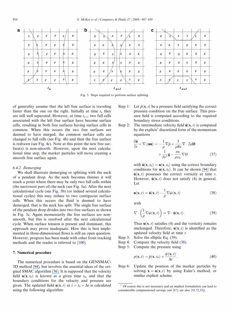
Fig. 5. Steps required to perform surface splitting.

1 Of course this is not necessary and an implicit formulation can lead toconsiderable computational savings (see [67]; see also [18,72,32]).

916 S. McKee et al. / Computers & Fluids 37 (2008) 907–930

of generality assume that the left free surface is travelingfaster than the one on the right. Initially at time tn theyare still well separated. However, at time tnþ1 two full cellsassociated with the left free surface have become surfacecells, resulting in both free surfaces having surface cells incommon. When this occurs the two free surfaces aredeemed to have merged, the common surface cells arechanged to full cells (see Fig. 4b) and then the free surfaceis redrawn (see Fig. 4c). Note at this point the new free sur-face(s) is non-smooth. However, upon the next calcula-tional time step, the marker particles will move creating asmooth free surface again.

6.4.2. Demerging

We shall illustrate demerging or splitting with the neckof a pendant drop. As the neck becomes thinner it willreach a point where there may be only two full cells within(the narrowest part of) the neck (see Fig. 5a). After the nextcalculational cycle (see Fig. 5b) (or indeed several calcula-tional cycles) this may reduce to two contiguous surfacecells. When this occurs the fluid is deemed to havedemerged, that is the neck has split. The single free surfaceof the pendant drop divides into two free surfaces as shownin Fig. 5c. Again momentarily the free surfaces are non-smooth, but this is resolved after the next calculationalcycle. When surface tension is present and dominant, thisapproach may prove inadequate. How this is best imple-mented in three-dimensional flows is still an open question.However, progress has been made with other front trackingmethods and the reader is referred to [100].

7. Numerical procedure

The numerical procedure is based on the GENSMAC-3D method [94], but involves the essential ideas of the ori-ginal SMAC algorithm [36]. It is supposed that the velocityfield uðx; t0Þ is known at a given time t0, and that theboundary conditions for the velocity and pressure aregiven. The updated field uðx; tÞ at t ¼ t0 þ Dt is calculatedusing the following algorithm:

Step 1: Let ~pðx; tÞ be a pressure field satisfying the correctpressure condition on the free surface. This pres-sure field is computed according to the requiredboundary stress conditions.

Step 2: The intermediate velocity field ~uðx; tÞ is computedby the explicit1 discretized form of the momentumequations

o~u

otþr:ðuuÞ ¼ � 1

qr~p þ 1

qRer � 2lD

þ 1

Fr2g� rj

qxerH ð37Þ

with ~uðx; t0Þ ¼ uðx; t0Þ using the correct boundaryconditions for uðx; t0Þ. It can be shown [94] that~uðx; tÞ possesses the correct vorticity at time t.However, ~uðx; tÞ does not satisfy (4) in general.Let

uðx; tÞ ¼ ~uðx; tÞ � 1

qrwðx; tÞ ð38Þ

with

� � r � 1

qrwðx; tÞ ¼ r � ~uðx; tÞ: ð39Þ

Thus uðx; tÞ satisfies (4) and the vorticity remainsunchanged. Therefore, uðx; tÞ is identified as theupdated velocity field at time t.

Step 3: Solve the elliptic Eq. (39).Step 4: Compute the velocity field (38).Step 5: Compute the pressure using

pðx; tÞ ¼ ~pðx; t0Þ þwðx; tÞ

Dt: ð40Þ

Step 6: Update the position of the marker particles bysolving _x ¼ uðx; tÞ by using Euler’s method, orsimilar explicit scheme.

S. McKee et al. / Computers & Fluids 37 (2008) 907–930 917

The last step in the calculation involves moving the markerparticles to their new positions. The coordinates of thesevirtual particles are stored and updated at each time stepby solving the differential equation dx=dt ¼ uðx; tÞ. Thisprovides the new coordinates of every particle, allowingus to determine whether or not it has moved to a new com-putational cell or it has left the containment region throughan outlet. By using the front tracking methodology [81],only marker particles on the free surface and the interfacesneed to be considered.

The elliptic Eq. (39) is solved using the conjugate gradi-ent method with the previous velocity field employed as theinitial guess. However, as the density variation across theinterface increases, more iterations are required for conver-gence of the method. In these cases, it is advisable to use adiagonal preconditioner to speed up the convergence of theconjugate gradient method.

The numerical procedure we have just described implic-itly assumes that we are dealing with Newtonian fluids. Thealgorithm extends fairly naturally to non-Newtonian fluids(and generalized Newtonian fluids, see [96]). Two furthersteps are required between step 4 an step 6, namely:

Step 5a: Update the components of the non-Newtonianextra-stress tensor on the rigid boundaries (formore detail, see [96]).

Step 5b: Compute the non-Newtonian extra-stress tensorS from Eq. (19)� �

Sþ We S

O

¼ 2 1� k2

k1

D: ð41Þ

Eq. (41) is solved by finite differences in an analogous wayto the Navier–Stokes equation. Details will not be givenhere, but it can be found in [92] for the two-dimensionalcase and in Tome et al. [97] for the three-dimensional case.

7.1. Time-stepping procedure

A time-stepping procedure for computing the appropri-ate time-step size for every cycle is employed. It is based onthe stability conditions (written in non-dimensional form)

Dt <Dx

kuk ; ð42Þ

Dt <Dx2Dy2Dz2

Dx2Dy2 þ Dx2Dz2 þ Dy2Dz2

Re2; ð43Þ

where the first inequality is understood componentwise.The restriction (42) requires that no particles should crossmore than one cell boundary in a given time interval; thisis an accuracy requirement. The second restriction (43)comes from the explicit discretization of the Navier–Stokesequations and is essentially a local von Neumann stabilityrequirement. Since low Reynolds number flows (0 6Re 6 10) are the primary concern, it is anticipated that(43) is generally the more restrictive condition.

Let Dtn be the time-step employed in the previous calcu-lational cycle and define

Dtvisc ¼1

2

Dx2Dy2Dz2

Dx2Dy2 þ Dx2Dz2 þ Dy2Dz2

Re2; ð44Þ

Dtu ¼ k1 �1

2� Dxjeumaxj

; ð45Þ

Dtv ¼ k2 �1

2� Dyjevmaxj

; ð46Þ

Dtw ¼ k3 �1

2� Dzjewmaxj

; ð47Þ

where j~umaxj, j~vmaxj and j~wmaxj are maximum of the tilde veloc-ities computed through (37) and 0 < ki 6 1; i ¼ 1; 2; 3. Theextra factor of 0.5 in (45)–(47) has been introduced as a con-servative measure to allow for the fact that only local stabil-ity analyses have been performed. The time-step employed inthe calculation is then chosen to be

Dtnþ1 ¼ k �minfDtvisc;Dtu;Dtv;Dtwg; ð48Þwhere 0 < k 6 1.

The factor k in (48) is necessary since the values of junþ1maxj,

jvnþ1maxj and jwnþ1

maxj at the beginning of the calculational cycleare not known. It is computationally more efficient to usethe tilde velocities with the factor k acting as a compensat-ing measure than using unþ1

max, vnþ1max, and wnþ1

max. However, ifDtu, Dtv or Dtw is less than Dtn then the tilde velocities arerecalculated and the time-step is revised. This time-steppingprocedure has proved to be an efficient automatic means ofadjusting the size of the time-step.

7.2. Finite difference approximation of the convective terms

For higher Reynolds numbers (Re � 1000) the convec-tive terms must be approximated by monotone, bounded,high accuracy upwinding. The upwinding scheme we haveselected to use is that due to Varonos and Bergeles [102](known as VONOS).

There are of course many others, but this proved to beone of the most effective when solving the hydraulic jumpproblem (see Section 12.3) – the reader is referred to thecomparison made by Ferreira et al. [23].

We require an approximation to the convective term,r � ðuuÞ, that is for the x component a bounded monotonehigh accuracy finite difference approximation is requiredfor

oðuuÞox

����iþ1

2;j;k

þ oðuvÞoy

����iþ1

2;j;k

þ oðuwÞoz

����iþ1

2;j;k

:

Since the VONOS scheme is complex and lengthy, it isomitted here; the reader may wish to consult the originalpaper [102] or Ferreira et al. [23] for details.

8. Undulation removal

The computation of the surface and interfacial tension isperformed at two levels: first at the sub-grid level, where

918 S. McKee et al. / Computers & Fluids 37 (2008) 907–930

small undulations in the fronts (free surfaces and inter-faces) are eliminated; and second at the cell level wherethe curvature at each surface or interface cell is approxi-mated. This approximation will be used in the implementa-tion of the pressure boundary condition at the free surfaceand in the calculation of the interfacial forces discussed inSection 8.3.

In many applications, in particular when the Reynoldsnumber is high (larger than 50), small undulations mayappear at the free surface and at the interfaces. This isdue to variations in the velocity field from cell to cell andmay be amplified in regions where the surface area isshrinking. They are physically removed by a combinationof surface and interfacial tension and viscous effects. Anumerical implementation that acts at cell level cannot takeinto account these sub-cell undulations and correctly sup-press then.

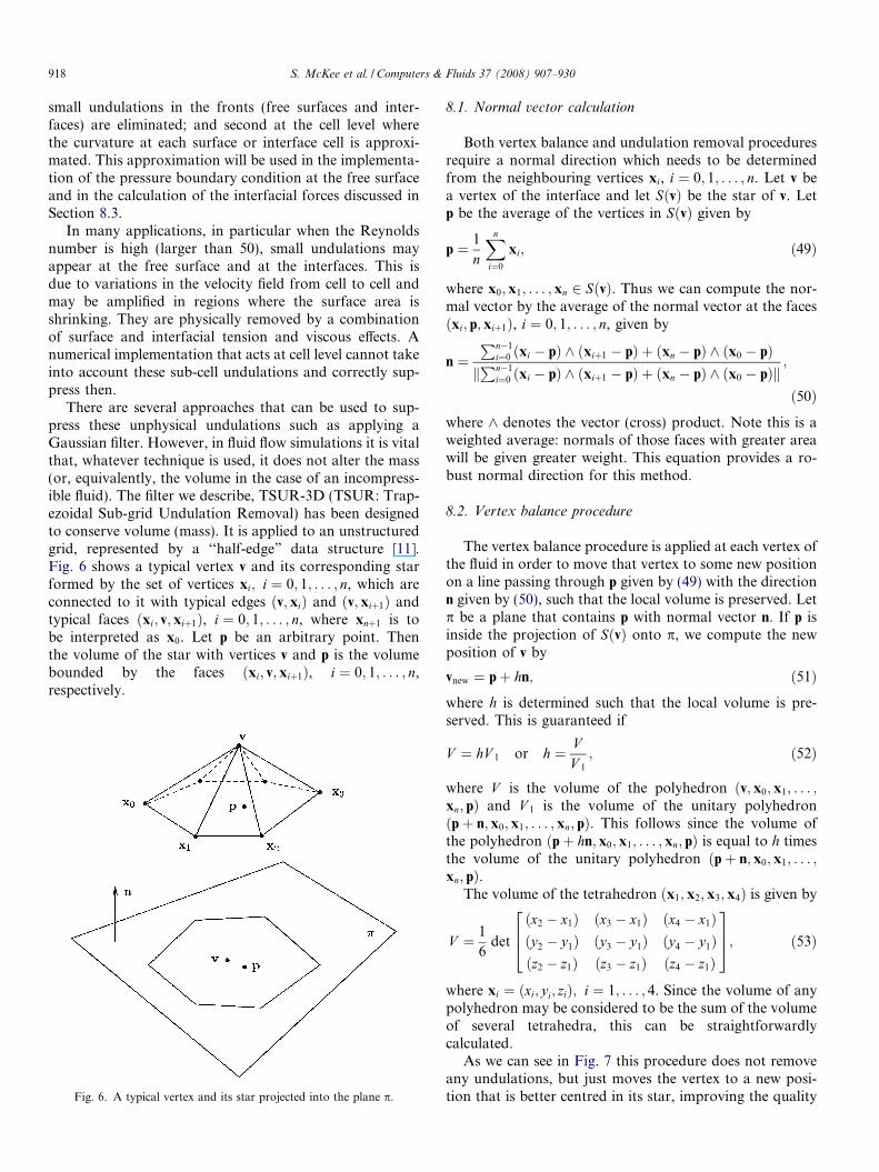
There are several approaches that can be used to sup-press these unphysical undulations such as applying aGaussian filter. However, in fluid flow simulations it is vitalthat, whatever technique is used, it does not alter the mass(or, equivalently, the volume in the case of an incompress-ible fluid). The filter we describe, TSUR-3D (TSUR: Trap-ezoidal Sub-grid Undulation Removal) has been designedto conserve volume (mass). It is applied to an unstructuredgrid, represented by a ‘‘half-edge” data structure [11].Fig. 6 shows a typical vertex v and its corresponding starformed by the set of vertices xi; i ¼ 0; 1; . . . ; n, which areconnected to it with typical edges ðv; xiÞ and ðv; xiþ1Þ andtypical faces ðxi; v; xiþ1Þ, i ¼ 0; 1; . . . ; n, where xnþ1 is tobe interpreted as x0. Let p be an arbitrary point. Thenthe volume of the star with vertices v and p is the volumebounded by the faces ðxi; v; xiþ1Þ, i ¼ 0; 1; . . . ; n,respectively.

Fig. 6. A typical vertex and its star projected into the plane p.

8.1. Normal vector calculation

Both vertex balance and undulation removal proceduresrequire a normal direction which needs to be determinedfrom the neighbouring vertices xi, i ¼ 0; 1; . . . ; n. Let v bea vertex of the interface and let SðvÞ be the star of v. Letp be the average of the vertices in SðvÞ given by

p ¼ 1

n

Xn

i¼0

xi; ð49Þ

where x0; x1; . . . ; xn 2 SðvÞ. Thus we can compute the nor-mal vector by the average of the normal vector at the facesðxi; p; xiþ1Þ, i ¼ 0; 1; . . . ; n, given by

n ¼Pn�1

i¼0 ðxi � pÞ ^ ðxiþ1 � pÞ þ ðxn � pÞ ^ ðx0 � pÞkPn�1

i¼0 ðxi � pÞ ^ ðxiþ1 � pÞ þ ðxn � pÞ ^ ðx0 � pÞk;

ð50Þwhere ^ denotes the vector (cross) product. Note this is aweighted average: normals of those faces with greater areawill be given greater weight. This equation provides a ro-bust normal direction for this method.

8.2. Vertex balance procedure

The vertex balance procedure is applied at each vertex ofthe fluid in order to move that vertex to some new positionon a line passing through p given by (49) with the directionn given by (50), such that the local volume is preserved. Letp be a plane that contains p with normal vector n. If p isinside the projection of SðvÞ onto p, we compute the newposition of v by

vnew ¼ pþ hn; ð51Þwhere h is determined such that the local volume is pre-served. This is guaranteed if

V ¼ hV 1 or h ¼ VV 1

; ð52Þ

where V is the volume of the polyhedron ðv; x0; x1; . . . ;xn; pÞ and V 1 is the volume of the unitary polyhedronðpþ n; x0; x1; . . . ; xn; pÞ. This follows since the volume ofthe polyhedron ðpþ hn; x0; x1; . . . ; xn; pÞ is equal to h timesthe volume of the unitary polyhedron ðpþ n; x0; x1; . . . ;xn; pÞ.

The volume of the tetrahedron ðx1; x2; x3; x4Þ is given by

V ¼ 1

6det

ðx2 � x1Þ ðx3 � x1Þ ðx4 � x1Þðy2 � y1Þ ðy3 � y1Þ ðy4 � y1Þðz2 � z1Þ ðz3 � z1Þ ðz4 � z1Þ

264375; ð53Þ

where xi ¼ ðxi; yi; ziÞ; i ¼ 1; . . . ; 4. Since the volume of anypolyhedron may be considered to be the sum of the volumeof several tetrahedra, this can be straightforwardlycalculated.

As we can see in Fig. 7 this procedure does not removeany undulations, but just moves the vertex to a new posi-tion that is better centred in its star, improving the quality

Fig. 7. A vertex with its star, before and after the vertex balanceprocedure has been applied.

S. McKee et al. / Computers & Fluids 37 (2008) 907–930 919

of the surface mesh while preserving local volume. As weshall see this improves the robustness of the undulationremoval procedure presented in the next section.

8.3. Undulation removal procedure

The vertex balance procedure is designed to produce amore homogeneous unstructured grid that represents thefree surface or interface. However, it cannot remove thesub-grid undulations; a smoothing procedure is requiredfor the effective removal of these undulations.

Let e be an edge of a surface and v1 and v2 its vertices asshown in Fig. 8. The smoothing procedure changes thepositions of v1 and v2 simultaneously in a such way thatthe local volume is preserved. Let n1 and n2 be the normalvectors computed by (50) at the vertices v1 and v2, respec-tively. We consider a normal vector at the edge e givenby the average of n1 and n2, namely:

n ¼ n1 þ n2

kn1 þ n2k2

:

Let m ¼ 12ðv1 þ v2Þ be the average of the vertices of the edge

e. We determine the heights h1 and h2 in the direction ofthis normal vector by

h1 ¼ hv1 �m; ni and h2 ¼ hv2 �m; ni; ð54Þ

where h�; �i denotes the inner (or dot) product. Next, wecompute the points p1 and p2 by

p1 ¼ v1 � h1n and p2 ¼ v2 � h2n: ð55Þ

Fig. 8. Undulation removal procedu

Thus, we have two polyhedra ðv1; x10; x11; . . . ; x1n; p1Þ withvolume V 1 and ðv2; x20; x21; . . . ; x2n; p2Þ with volume V 2,where ðx10; x11; . . . ; x1nÞ 2 Sðv1Þ and ðx20; x21; . . . ;x2nÞ 2 Sðv2Þ (see Fig. 8). We have to determine the new heighth in the direction of n such that the local volume is preserved.

We can exploit linearity between volumes of polyhedraand their heights by writing

V 1 þ V 2 ¼ V 1ðh=h1Þ þ V 2ðh=h2Þ ð56Þor

h ¼ V 1 þ V 2

V 1=h1 þ V 2=h2

: ð57Þ

The new positions of the vertices v1 and v2 are given by

v1 ¼ p1 þ hn and v2 ¼ p2 þ hn: ð58ÞThis undulation removal procedure is applied periodicallyto all the edges of the surface mesh with a period thathas to be chosen such that the surface is sufficientlysmooth, and the large scale undulations are not greatly af-fected. The frequency of application is dependent on theparticular problem, the grid resolution and the time step.Of course,this undulation removal procedure and the cur-vature calculation of the next section need not be appliedto a large class of problems – non-Newtonian low Rey-nolds number flows, especially when surface or interfacetension can be neglected.

9. Curvature calculation

The curvature is approximated by the surface that bestfits the points (the positions of the marker particles) in thatcell and its neighbours. Numerical experimentation (see[80,81]) suggests approximation by the paraboloid

pðx; yÞ ¼ ax2 þ bxy þ cy2 þ dxþ ey þ f : ð59ÞIn this approximation, we first need to determine the nor-mal vector at the cell centre. We can summarize the methodof curvature approximation by the following steps:

1. Given a surface at an interface cell, consider all pointsthat lie inside a sphere Sd with its centre at the cell centreand a given radius d.

2. Fit a plane to these points and compute its normal.3. Take a new coordinate system normal to the surface

using the computed normal from the second step.

re, showing an edge and its star.

920 S. McKee et al. / Computers & Fluids 37 (2008) 907–930

4. Consider a new sphere S�, centred at the cell centre, witha specified radius � and then map the points in thissphere to the new coordinate system.

5. In the new coordinate system compute the coefficients ofthe surface given by (59).

6. Compute the curvature of the fitted surface using

j ¼o2pon2

1þ ðopon Þ

2� 3=2

þo2pog2

1þ ðopog Þ

2� 3=2

; ð60Þ

where p is the fitted surface given by (59) and ðn; g; fÞ arethe coordinates of the new coordinate system. Note thef-axis is parallel to the normal vector.

In this method, the quality of the approximation is directlyrelated to the chosen radii d and �. Typically, d is chosen tobe of the order of a cell size and �, 1.5 times larger. Formore detailed discussion of the influence of these constantssee [81], where the optimum choice for these numbers isdiscussed.

How the normal vector and the curvature approxima-tions are made will be described in detail in the next sub-section.

9.1. Normal vector approximation

The region Sd associated with the cell S will include anumber of points (coordinates of the marker particles).Let that number be m ¼ mðdÞ. Let xi ¼ ðxi; yi; ziÞ,i ¼ 1; 2; . . . ;md, be the number of points inside Sd and thusthe number of points in cell S and its surrounding neigh-bours. The equation of the plane will be eitherz ¼ f ðx; yÞ, y ¼ f ðx; zÞ or x ¼ f ðy; zÞ, according to the max-imum absolute value of the cell normal vector components.For example, if

jhnC; ð0; 0; 1Þij > jhnC; ð1; 0; 0Þij and jhnC; ð0; 0; 1Þij> jhnC; ð0; 1; 0Þij;

where h�; �i denotes the inner product, the equation of theplane is given by z ¼ f ðx; yÞ ¼ axþ by þ c and the coeffi-cients a, b and c are then determined as a best least squaresfit to the given points. The normal vector to the planez ¼ axþ by þ c can then be calculated from

ns ¼ða; b;�1Þkða; b;�1Þk2

: ð61Þ

The other cases follow similarly. This procedure determinesns, but the sign may be incorrect. The correct sign can bedetermined by comparing ns with the normal at the cell cen-tre nc, previously obtained (Section 6.2). If hnC; nSi > 0 thesign is correct; otherwise the sign must be reversed.

9.2. Curvature approximation

Now let xi ¼ ðxi; yi; ziÞ, i ¼ 1; 2; . . . ;m�, be the pointslying in S�. With the normal vector ns given by the plane fit-

ting technique of Section 9.1, we choose another two tan-gent vectors at the surface such that they form anorthonormal basis together with the normal vector. Firstwe choose two of the three canonical vector e1 ¼ ð1; 0; 0Þ,e2 ¼ ð0; 1; 0Þ and e3 ¼ ð0; 0; 1Þ whose projections on thedirection of ns vector are smallest. Second, we apply theGram Schmidt method to obtain an orthonormal basis.Thus, we have a new coordinate system and the points xi

can be expressed in terms of this new coordinate systemas ni ¼ ðni; gi; fiÞ. This, then, allows us to fit the paraboloid

pðn; gÞ ¼ an2 þ bngþ cg2 þ dnþ egþ f

using least squares. This gives us the ‘‘best-fit” values for a,b, c, d, e and f from whence we obtain the curvature

j ¼ �2a

ð1þ d2Þ3=2þ b

ð1þ e2Þ3=2

!: ð62Þ

10. A dynamic contact angle

When two fluids, in this case water and air, meet at asolid surface they meet at an angle that is generally not nor-mal to that surface. This is called the contact angle and ifthe fluids are not quiescent then this angle will move. ThisSection is concerned with how the MAC method can trackthis moving contact angle.

The contact angle will have the effect of influencing thecurvature in the surface cells adjacent to the boundarycells. Thus these surface cells will not be employed directlyin the computation of the curvature. Instead the curvaturein this case is estimated using the free surface normal n1,computed at the point x1 of the surface in the adjacent cellopposite to the wall; the coordinates of x1 were previouslyobtained using the methods of Section 6.1, using the nor-mal to the free surface at the wall (which is prescribed inthe case of a constant angle) and the normal distance bof x1 from the wall. The details of the method may becomesomewhat clearer by referring to the situation depicted inFig. 9, which displays, for clarity, the equivalent two-dimensional problem. Again for simplicity of exposition,we shall, in the following, restrict ourselves to two dimen-sions. Generalization to three dimensions should be clear.

Let S1 be a surface cell adjacent to a boundary cell B forwhich we need to compute the capillary pressure. Let n1 bethe free surface (interface) unit normal, computed at thecentre x1 of the adjacent surface cell S2. Let n3 be the wallunit normal, and let n2 be the free surface (interface) unitnormal at the contact point which is obtained by addingthe (prescribed) contact angle / to the wall angle. Let sw

be the unit vector tangent to the wall. Finally, let ss bethe unit vector tangent to the free surface at the point ofcontact x2 at the current time t. The point of contact at aprevious time t ¼ t � Dt will be denoted by x2.

If the direction of the outward normal is specified, thena circle may be uniquely defined by its radius and one pointon its circumference. Consider then the circle passing

Fig. 9. Method for the approximation of the contact angle.

S. McKee et al. / Computers & Fluids 37 (2008) 907–930 921

through x1 and x2 with radius r. If the outward unit normalat x1 is n1 then this uniquely determines its centre which weshall denote by x0. The two main identities followimmediately:

x1 � x0 ¼ rn1; x2 � x0 ¼ rn2:

Therefore

x1 � x2 ¼ rðn1 � n2Þ: ð63Þ

On the other hand, if b denotes the normal distance fromx1 to the wall, we have that

b ¼ ðx1 � x2Þ � n3: ð64Þ

Hence, on substituting (63) into (64), we obtain

rðn1 � n2Þ � n3 ¼ b ð65Þand then

j ¼ 1

r¼ ðn1 � n2Þ � n3

b: ð66Þ

We do not explicitly impose a slip boundary condition atthe contact line. For B-cells adjacent to a S-cell we applystandard no-slip boundary conditions, and that the com-puted capillary pressure is applied at the S-cell. This isdue to the fact that the slip region is interpreted as re-stricted to a microscopic region in the proximity of the con-tact point, while in most of the B-cell the no-slip conditionswill still prevail. Therefore, the position of the marker par-ticles, which should be updated using the contact pointvelocity, will not be correct close to the wall. Hence, forthe analysis of the results, the position of the surface givenby the tracking points at the cell closest to the wall are onlyapproximate and may be disregarded, while the effectiveextension of the free surface and the contact point are givenby the approximation described in this Section. The above

procedure is quite general and, in principle, can be appliedto impose any contact angle.

In the case of a dynamic contact angle, the value of thecontact angle can be determined empirically using ‘‘Tan-ner’s law” (see [85,86])

uc ¼ F ðuÞ; ð67Þ

where uc is the velocity of the contact point in the directionof the wall and u is the contact angle related to the surfaceand wall normals given by

cosðuÞ ¼ n2 � n3: ð68Þ

One simple approximation for F ðuÞ is given by

F ðuÞ ¼ a0 þ a1u ð69Þ

for given constants a0 and a1.Recall that x2 is the contact point position at a previous

time, say t � Dt, the velocity of the contact point uc may beestimated using a first-order approximation

uc ¼ðx2 � x2Þ � sw

Dt; ð70Þ

where the direction of sw is determined by imposingsw � n2 > 0. The curvature, therefore, can be calculated bysolving (65)–(69).

A simple, but effective procedure is as follows. Firstcompute b directly from (65). Use the old value of uc asan initial guess and compute u from (67) with (69). Use(65) and (68) to determine r ¼ 1=j and n2. Eq. (66) isnow checked to see if it is satisfied. If not, then a bisection(or other root finding) algorithm may be used until uc hasbeen found to sufficient precision. Eq. (70) may then beused to calculate x2. For low Reynolds number simulation,when Dt is small due to viscous stability restrictions, correc-tion steps are not required.

11. Data structure and system environment

11.1. Data structure

Freeflow-3D uses two classes of data: direct and indirectdata. The first class contains the data concerning thedomain, velocities, pressure, cells, parameters used by thesimulator (Simflow-3D) and the representation of geomet-ric objects of the model. The direct data set is subdividedinto two sub-classes, namely, static and dynamic data.The static data comprise the data defining the domain,the discretization, the non-dimensionalization parametersand the time-independent fluid properties (e.g. viscosity).The dynamic data comprise data concerning velocities,pressure, cell type and the representation of geometricobjects. Velocity and pressure are stored as matrices. Thecells are represented by a matrix and, additionally, thosecontaining fluid, or on the rigid boundary, are also storedin a tree-like data structure. The reason for having someof the cells represented twice is because access to specificgroups of cells, namely F, S, B and I cells, is required

922 S. McKee et al. / Computers & Fluids 37 (2008) 907–930

throughout the code and in this case tree storage is muchmore efficient. On the other hand, when access to all cellsor to adjacent cells is required a matrix representation faresbetter. Moreover, further information can be built into thetree representation, improving the performance of thecode. For instance, for a S cell the normal vector needsto be stored, whereas for a boundary cell the intersectionsof the grid lines with the container surface arerequired.

The geometric objects have their surfaces approximatedby piecewise linear surfaces and so are represented by ahalf-edge data structure which is a B-Rep (Boundary Rep-resentation) [58] structure. This structure is used to repre-sent faces, edges, vertices and their topologicalrelationships. It was originally designed to model rigid sol-ids from a knowledge of their surfaces. The insertion anddeletion of data into the half-edge data structure are madeby the Euler operators which also guarantee the consis-tency of the represented object. Among other types of rep-resentations of solids (e.g. Constructive Solid Geometry,Spatial Occupancy Enumeration, Cell Decomposition[58]), the B-Rep representation was chosen because of itsconciseness, its explicit representation of the boundary sur-face and its capability to efficiently perform local modifica-tions to the object’s surface.

The data structure employed to represent the class ofindirect data was constructed with three main points inmind: the representation of geometric objects by their sur-faces, the performance of the algorithms involved in thesimulation, and the minimization of interdependency ofthe data. The indirect data consists of two types, calledContainers, Inflows and Outflows, representing containers,inflows and outflows, respectively. The Container datastructure is composed of geometric data (B-Rep), bound-ary condition types, information stored in a tree structureabout the cells that define the container and specific attri-butes of the container. In addition, the container can moveby prescribing trajectories such as harmonic motion, rota-tional motion, piecewise linear trajectories, splines trajecto-

ries and movements defined by external forces. Thesetypes of movements are stored in the Container datastructure.

The Inflow data structure is composed of geometric data(B-Rep), inflow properties, information about the con-tainer and the fluid related to the inflow, and a tree struc-ture storing information about the cells defining the inflowand specific attributes concerning the inflow. Like the con-tainers, the inflows can move by prescribing the trajectoriesof harmonic motion, piecewise linear trajectories and splines

trajectories. The information about the inflow movement isstored in the Inflow data structure.

The Outflow data structure is also composed of geomet-ric data (B-rep) and outflow properties such as its plane ofdefinition and orientation.

The data structures described above are used by Mod-flow-3D to build the initial configuration for the flow thatwill then be evolved by Simflow-3D.

11.2. The module Modflow-3D

Modflow-3D is responsible for data initialization of thesimulation module. It consists of an user-friendly graphicinterface for data input related to the flow, such as thedomain, mesh, cells, reference values, flow type, parame-ters, error tolerance used by the simulation module andgeometric objects making up the model. Modflow-3D alsopermits the visualization of the entered data. The techniqueused for viewing objects is rendering which makes it easierfor the user to interpret what he sees. In addition to theusual geometrical operations like rotation, translationand zoom, the user can choose the type of projection (par-allel, perspective), the viewer’s distance, the rendering type(e.g. Wire-frame, Flat, Gouraud, Phong) and ambientaland directional light intensity. Another useful feature ofthis module is the possibility of altering object visualizationproperties like color, visibility, transparency and lightreflection properties.

The geometric objects are represented using the half-edge B-Rep data structure, and this representation isachieved using a well known modeling technique: three-dimensional primitive instancing. The technique of primi-tive instancing permits the choice of objects from a menuof pre-defined objects by simply defining their parameters.Currently, there are several choices, such as open rectangu-lar (trapezoidal) boxes, open cylindrical/conical boxes,solid sphere, solid cylinder, pipe, solid square torus andso on.

The remaining data in the structures Container, Inflow,Outflow and Fluid are directly obtainable from a pull-down menu. For instance, the structure Inflow also con-tains information on: inflow plane and inflow orientation,inflow velocity, boundary condition type, parameters forparticle insertion (number of particles in each direction ineach cell), a tree storing the cell set defining the inflow dis-cretization and specific attributes of the inflow. The inflowscan be of type Linear or Parabolic. The inflow type Linearis defined by having a constant velocity profile while theParabolic inflow has a parabolic velocity profile. Like thestructure Inflow, the structure Outflow contains informa-tion about outflow plane and outflow orientation. The spe-cific attributes are data such as: visualization parameters,and data related to the nozzle definition and movement.

11.3. The module Simflow-3D

The module Simflow-3D is the central part of the simu-lation environment described in this article because itimplements the governing equations and boundary condi-tions. One of the main challenges in generalizing the ideasof the two-dimensional code, GENSMAC [88], to threedimensions was in dealing with the free surface. This wasbecause in two dimensions virtual particles were used torepresent the fluid, and this technique could not have beencarried over to three dimensions due to the very large num-ber of particles that would have been needed to represent

S. McKee et al. / Computers & Fluids 37 (2008) 907–930 923

the fluid to photographic precision. We resolved this prob-lem by introducing a new procedure whereby marker par-ticles were only employed on the surface of the fluid.This brought huge savings in storage and computing timemaking the extension of GENSMAC feasible for solvingfull three-dimensional problems efficiently.

11.4. The module Visflow-3D

Visflow-3D is responsible for the presentation of theoutput produced by Modflow-3D and Simflow-3D. Thisoutput comprises data from the flow model, object repre-sentation and properties of the flow saved at pre-definedinstants of time. Time-independent data are stored in a sin-gle file, while those which are time-dependent are stored ina sequence of files containing information about the geom-etry of objects, the flow properties, cell configuration, timeand cycle number. Visflow-3D allows the user to view thegeometry (containers, inflows and outflows), the fluid flowitself and also the flow properties (velocity, pressure, vis-cosity, shear rate and stress tensor components). LikeModflow-3D, Visflow-3D uses rendering techniques forobject presentation in order to make user-understandingof the pictures more immediate.

In addition to the viewing facilities provided by Mod-flow-3D, the user can view cuts of objects by planes parallelto one of the main axes or planes parallel to a user defineddirection. Flow properties can be viewed in three dimen-sions using rendering techniques by considering the flowproperty as a texture, or they can be viewed as contourlines. Both the velocity and the stress tensor can be visual-ized through its components; for instance, the velocity canbe understood by exhibiting its components u, v and w

while the stress tensor can be interpreted by viewing itscomponents Sxx; Sxy ; . . . ; Szz.

11.5. Communication between the modules

Communication between modules is carried out throughfiles. Modflow-3D outputs six files: three of them storeinformation on the half-edge structure of containers,inflows and fluids. Two files store information on the indi-rect structure of containers and inflows, and the sixth filestores all the remaining data such as viscosity, time-stepfactors, time-step size, scaling parameters, flow properties,etc. The module Simflow-3D has, as input, six files all withthe same structure as the output files of the module Mod-flow-3D. These files may have been created either by Mod-flow-3D or by Simflow-3D. The output files of Simflow-3Dhave four different purposes: normal exit – creates files forcontinuing the simulation if desired; forced exit – files cre-ated if an error occurs, this aids debugging; pre-definedtemporary saves – for the event of a system crash; andfinally, visualization files – for viewing the results. In thefirst three cases the files have the same structure as thoseof Modflow-3D; in the last they have the structure of Vis-flow-3D. The input for the module Visflow-3D is created in

three files containing information on the half-edge struc-ture of containers, inflows and fluids. These files are usedfor visualizing the objects. An additional five files, contain-ing the values of the velocity and pressure fields u, v, w, p

and the configuration of the cells, are created for visualiz-ing the flow properties. A further file containing time-inde-pendent data (called the manager) is created at thebeginning of the simulation and is used throughout.

12. Applications

We conclude this paper by presenting numerical simula-tions of three-dimensional free surface flows.

12.1. Jet buckling

When a cylindrical jet flows onto a rigid surface a phe-nomenon known as jet buckling can occur if the Reynoldsnumber is smaller than a prescribed value. This flow hasattracted the attention of a number of researchers andhas been studied both experimentally and numerically byCruickshank and Munson [15] and Cruickshank [16]. Theypresented results, both experimental and theoretical, forNewtonian jets. From their study, they obtained estimatesfor when jet buckling occurs. These are based on the Rey-nolds number and the aspect ratio H=D, where H is theheight of the inlet to the rigid plate and D is the jet diam-eter. For an axisymmetric jet, they found that if the condi-tions Re < 1:2 and H=D > 7:0 were satisfied then the jetwould buckle. In order to simulate this problem, we consid-ered a cylindrical thin jet of diameter D ¼ 6 mm issuingfrom an inlet situated at a height H ¼ 5 cm above the plate(so that H=D 8:33) flowing onto a rigid plate. A uniforminput velocity of U ¼ 1 m s�1 was set at the inlet, and thefluid viscosity m ¼ 0:012 m2 s�1 was used. Surface tensionwas neglected. The scaling parameters were U ;D; m so thatRe ¼ 0:5 and 1=F 2

r ¼ 0:242611. A mesh size of Dx ¼ Dy ¼Dz ¼ 0:001 mm (85� 85� 155) was employed. Fig. 10 dis-plays the fluid flow configuration at different times. Fig. 11also displays the equivalent fluid flow configuration for aplanar jet.

12.2. Splashing drop

A spherical drop of fluid of diameter D ¼ 10 mm isgiven an initial velocity of U ¼ 1 m s�1 and released froma height of 4 cm above a square container containing a qui-escent fluid. The value of the viscosity was m ¼ 10�6 m2 s�1

so that the Reynolds number Re ¼ UD=m ¼ 1; 000. Themesh used in this example was 100� 100� 100 cells(Dx ¼ Dy ¼ Dz ¼ 1:0 mm). The initial indentation may beobserved with the formation of a traveling wave. Highpressure beneath this indentation causes fluid to travelupwards (in the form of a splash). As the ‘‘splash” reachesits peak we can observe the surface waves being reflectedfrom the sides of the container (see Fig. 12). In this

Fig. 10. Three-dimensional numerical simulation of cylindrical jet buck-ling at different times.

Fig. 11. Three-dimensional numerical simulation of planar jet buckling atdifferent times.

Fig. 12. Three-dimensional numerical simulation the splashing drop atdifferent times.

Fig. 13. Three-dimensional numerical simulation of a circular hydraulicjump at different times.

924 S. McKee et al. / Computers & Fluids 37 (2008) 907–930

problem surface tension is insignificant (see, for example,[51]) and was neglected.

12.3. Hydraulic jump

The Freeflow3D code has been applied to simulate a cir-cular hydraulic jump. We considered a cylindrical jet of aviscous fluid flowing rapidly onto a rigid horizontal sur-face. The non-dimensional parameters were: Re ¼ 400,Fr ¼ 1:785. The scaling parameters were: inflow velocity

U ¼ 0:5 m s�1, inflow diameter D ¼ 8:0 mm and kinematicviscosity m ¼ 10�5 m2 s�1. Gravity was considered to be act-ing in the z-direction with g ¼ �9:81 m s�2. The mesh usedin this example was 100� 100� 100 cells (Dx ¼ Dy ¼Dz ¼ 1:0 mm). The Freeflow3D code solved this problemwith the above input data. Fig. 13 exhibits snapshots of thisrun at selected times. Surface tension has been neglected.

12.4. Rising bubbles

This example displays the simulation of three phase fluidflow of two bubbles with different densities, viscosities anddiameters, rising in a third phase with a greater density.The bubbles rise due to buoyancy forces. The non-dimen-sional parameters were: Re ¼ 55:75, Fr ¼ 1, xe ¼ 4:6. Forthe continuous phase, qf ¼ 880 kg=m3 and lf ¼ 0:0125 Ns=m2. For the larger bubble, D1 ¼ 4 mm, q1 ¼ 88 kg=m3

and l1 ¼ 0:00125 N s=m2, with Eo1 ¼ 4:6. Finally, for thesmaller bubble, D2 ¼ 2 mm, q2 ¼ 176 kg=m3 and l2 ¼

S. McKee et al. / Computers & Fluids 37 (2008) 907–930 925

0:0025 N s=m2, with Eo2 ¼ 1:15. The surface tension coeffi-cient for all interfaces was chosen to be rI ¼ 0:03 N=m.The lengths and velocities were non-dimensionalized usingD1 ¼ 4 mm and U ¼

ffiffiffiffiffiffiffiffigD1

p, respectively. The grid used in

this example was 32� 32� 64 cells. Fig. 14 displays thetime evolution of the flow. It can be seen that the largerbubble undergoes a larger deformation than the smallerbubble, due to its larger Eotvos number (Eo ¼ qgD2r�1).There is a small deflection in the trajectory of the smallerbubble as a result of the interaction with the larger bubbleas it passes by. Surface tension plays an important role.

12.5. Container filling

We present a calculation which simulates the fillingbehavior of a trapezoidal container with a rectangular noz-

Fig. 14. Two bubbles rising in a continuous phase, at different times.

Fig. 15. Simulation of the filling process of a trapezoidal container atdifferent times.

zle. The following input data were employed: The non-dimensional parameters were: Re ¼ 7:5, Fr ¼ 2:9146. Thescaling parameters were: velocity reference valueU ¼ 1:0 m s�1 (fluid velocity at the nozzle), length referencevalue L ¼ 12:0 mm (jet width in the x-direction), and kine-matic viscosity 1:6�3 m2 s�1. Gravity was assumed to beacting in the z-direction with g ¼ �9:81 m s�2. The meshused in this example was 80� 120� 70 cells(Dx ¼ Dy ¼ Dz ¼ 1:0 mm). The Freeflow3D code solvedthis problem with the above input data. Fig. 15 displaysa series of snapshots taken during this run.

13. Viscoelastic flows

13.1. Oldroyd-B

Complex fluids such as polymer melts and solutions,suspensions and micelle solutions are encountered in anvariety of industries and applications critical to modernday economies, and a fundamental understanding of theirbehavior is becoming increasingly important. There aremany models of viscoelasticity; the reader is referred tothe recent book by Owens and Phillips [68]. In this Sectionwe focus attention on just one, the Oldroyd-B model. Thiscan be characterized by the equations of mass and momen-tum conservation (4) and (5) and its constitutive equation

sþ k1 s5 ¼ 2l Dþ k2 D

5� �

; ð71Þ

where k1 and k2 are the relaxation and retardation timeconstants.

13.2. Elastic jet

To illustrate the effect of viscoelasticity on the bucklingphenomenon we applied Freeflow3D to simulate thin jetsflowing onto a rigid plate. We considered a rigid plate ofdimensions 6 cm � 6 cm and an axisymmetric nozzle situ-ated 12 cm above the rigid plate. The nozzle radius wasR ¼ 3 mm and the velocity of the jet issuing from the nozzlewas 1 m s�1. Two simulations were performed: one runwith a Newtonian jet and another run using a viscoelasticjet modeled by the Oldroyd-B constitutive equation. Thefluid properties were q ¼ 1; 000 kg=m3, l0 ¼ 0:004615Pa s, k1 ¼ 0:006 s, k2 ¼ 0:0006 s. Therefore we hadRe ¼ qUR=l0 ¼ 1:3 and We ¼ k1U=R ¼ 1. A mesh size of60 � 120 cells was employed in both simulations. We antic-ipated that the Newtonian jet will not buckle as the restric-tion Re < 1:2 is not satisfied (see Section 12.1). The resultsare displayed in Fig. 16 showing the jet flowing onto a rigidplate at different times. The Newtonian jet flows radiallywithout any sign of the buckling instability while the jetmodeled by the Oldroyd-B constitutive equation doesundergo slight buckling. The reason why the Oldroyd-Bjet buckles may be because of the extensional viscositywhich increased after the jet impinges upon the rigid plate.

Fig. 17. Fluid flow visualization at different times of the simulation of the extrudate swell for increasing values of Weeffect.

Fig. 16. Numerical simulation of jet impinging onto a rigid plate at different times. (a) Newtonian jet; (b) viscoelastic jet modeled by the Oldroyd-B model.

926 S. McKee et al. / Computers & Fluids 37 (2008) 907–930

S. McKee et al. / Computers & Fluids 37 (2008) 907–930 927

13.3. Die-Swell

We also applied the Freeflow3D code to the simulationof the extrudate swell of an Oldroyd-B fluid. The time-dependent flow of an axisymmetric jet flowing inside a tubeand then extruded in air was considered. The no-slipboundary condition is imposed on the tube walls, whilefully developed flow is assumed at the tube entrance. Onthe fluid free surface, the full stress conditions are applied.To simulate this problem the following input data wereemployed: tube radius R ¼ 1 cm, tube length L ¼ 3R,Dx ¼ Dy ¼ Dz ¼ 0:1 cm (20� 100� 100 cells). The fluidwas characterized by m0 ¼ 0:010 m2 s�1, k1 ¼ 0:01 s. Thescaling parameters were R, U ¼ 1, m0 and k1, givingRe ¼ UR=m0 ¼ 1 and We ¼ k1U=R ¼ 1. To demonstratethat the code can deal with the Oldroyd-B model, we usedthese input data and performed three simulations. In thefirst simulation the value of k2 ¼ 0:9k1 was used and inthe second simulation we used k2 ¼ 0:70k1 while in thethird simulation we chose k2 ¼ 0:5k1. Recall that the effec-tive Weissenberg number for the Oldroyd-B model is givenby (see [105]) Weeffect ¼ ð1� k2

k1ÞWe. Thus, in these simula-

tions we used Weeffect ¼ 0:1; 0:30; 0:5, respectively. Fig. 17shows the jet flowing inside the tube and then beingextruded into the air. For the time t ¼ 0:04s (first column)the jet is just leaving the tube and the differences betweenthe three simulations are not noticeable, at least to thehuman eye. However, at later times the jet is extruded intothe air and the differences between the three simulationsbecome clearer. This is particularly true for the case oft ¼ 0:12 s (last column), where we can observe that theresults for the case of Weeffect ¼ 0:5 present a much largerswelling than that of the other two simulations. Indeed,at the time t ¼ 0:12 s, the maximum swelling ratios(Sr ¼ Rmax=R) for the three simulations were 28% forWeeffect ¼ 0:1, 46% for Weeffect ¼ 0:30 and 59% forWeeffect ¼ 0:5.

14. Future developments

One of the attractive features of the MAC method is itssimplicity: a fixed Eulerian grid is used – it does not ‘suffer’from the complexity of adaptivity; finite difference meth-ods are employed and these, for the most part, are at mostsecond order; robustness is achieved through the use ofsmall, often very small time steps especially in the case oflow Reynolds number flows; the conjugate gradient solvertends to converge rapidly without the need for a precondi-tioner. Today, this ‘toy’ method of the 1960s has alreadybecome a useful scientific and technological tool, able tocompute quite large three-dimensional problems on gridsof the size of 1,000,000 computational cells using a modestcomputer and to display the results as a realistic videosequence. Tomorrow’s computers should make possiblecomputations over 1,000,000,000 computational cells.However, greater computing power itself may not be suffi-cient. One can think of many problems where this is true:

one such problem is that of bubbles rising in a beer glass –this could not be properly achieved with a billion compu-tational cells (unless, of course, the bubbles were treated asa continuum). We have seem that in order to computehigher Reynolds number flows it was found necessary toemploy high order monotone upwinding for the convectiveterms. In the future it will probably be necessary to sacri-fice the essential simplicity of the MAC approach andintroduce adaptivity and higher order methods or indeedother numerical methods such as finite elements or spectralcollocation. The ultimate goal is virtual reality computa-tional fluid dynamics (VRCFD) whereby the output is, ide-ally, in the form of a dynamic hologram (preferably in realtime) which is essentially indistinguishable from the ‘‘realthing”.

In Section 3 we presented a brief description of the vol-ume of fluid approach, the level set method and several dif-ferent front tracking techniques for solving free surfaceflow problems. Many codes have been written describingthe many variants (and hybrid variants) of the above.These codes are necessarily complex and it is becomingincreasingly difficult to compare one with the other, andthereby come to some kind of conclusion as to which isthe best. Indeed the word ‘best’ may have little meaninghere, as one code may be excellent at solving bubbly flowwhile another may be particularly effective when employedto compute viscoelastic flows. Nonetheless, it behoves theCFD community, in particular that large subset interestedin free surface flows, to attempt a systematic interrogationof all existing codes (and their underlying methods). Oneway to do this is for the community to agree on a set of testproblems that all good codes should be able to solve. Mostof us have experienced using a commercial code that didnot live up to the vendor’s claims: such codes, if subjectedto the test set, could be pinpointed and discounted.

To initiate this discussion the authors would like to con-clude by proposing six test problems that all ‘good’ codesshould be able to solve:

1. 3D jet buckling (Newtonian and viscoelastic).2. 3D splashing drop (Newtonian and viscoelastic): tung-

sten ball dropped from different heights – various con-figurations showing satellite drops from the resultantsplash.

3. 3D extrudate swelling (Newtonian and viscoelastic).4. 3D bursting bubble: a bubble bursting at the surface of a

fluid giving rise to a jet or a splash from its base.5. A large number of bubbles (>100, say) of different sizes,

densities and viscosities rising (and interacting) in afluid.

6. Rod climbing of a viscoelastic fluid at moderate Weiss-enberg number.

We suspect that not many existing codes could solvethese six problems. The MAC method, as described in thisarticle, cannot as yet, but we can foresee it being able to doso in the relatively near future.

928 S. McKee et al. / Computers & Fluids 37 (2008) 907–930

Acknowledgements

We acknowledgment support from the FAPESP (Fun-

dac�ao de Amparo a Pesquisa do Estado de Sao Paulo), Con-tract No. 04/16064-9. The second author has beensupported by CNPq (Conselho Nacional de Desenvolvimen-to Cientıfico e Tecnologico) under Grants Nos. 302048/2004-9, 504622/2003-0 and CAPES/GRICES Grant No.136/5.

References

[1] Amsden A, Harlow F. The SMAC method: a numerical techniquefor calculating incompressible fluid flows. Technical Report LA-4370, Los Alamos National Laboratory, 1970.

[2] Aulisa E, Manservisi S, Scardovelli R, Zaleski S. A geometricalarea-preserving volume-of-fluid advection method. J Comput Phys2003;192:355–64.

[3] Aulisa E, Manservisi S, Scardovelli R. A surface marker algorithmcoupled to an area-preserving marker redistribution method for three-dimensional interface tracking. J Comput Phys 2004;197:555–84.

[4] Baker GR, Moore DW. The rise and distortion of a two-dimensional gas bubble in an inviscid liquid. Phys Fluids A1989;9:1451–9.

[5] Bird RB, Armstrong RC, Hassager O. Dynamics of polymericliquids. Fluid mechanics, 2nd ed., vol. I. New York: John Wiley &Sons; 1967.

[6] Boulton-Stone JM, Blake JR. Gas bubbles bursting at a free surface.J Fluid Mech 1993;254:437–66.

[7] Brackbill JU, Ruppel HM. FLIP: a method for adaptively zoned,particle-in-cell calculations of fluid flows in two dimensions. JComput Phys 1986;65:314–43.

[8] Brackbill JU. The ringing instability in particle-in-cell calculationsof low-speed flow. J Comput Phys 1988;75:469–92.

[9] Brackbill JU. FLIP MHD: a particle-in-cell method for magneto-hydrodynamics. J Comput Phys 1991;96:163–92.

[10] Butler TD, O’Rourke PJ. A numerical method for two-dimensionalunsteady reacting flows. In: Sixteenth international symposium oncombustion. 1976. p. 1503–15.

[11] Castelo A, Tome MF, Cesar CNL, McKee S, Cuminato JA.Freeflow-3D and integrated simulation system for three-dimensionalfree surface flows. J Comput Visual Sci 2000;2:199–210.

[12] Chenn I-L, Glimm J, McBryan O, Plohr B, Yaniv S. Front trackingfor gas dynamics. J Comput Phys 1986;62:83–110.

[13] Craik AD, Latham RC, Fawkes MJ, Gribbon WF. The circularhydraulic jump. J Fluid Mech 1981;112:347–62.

[14] Cross MM. Rheology of non-Newtonian fluids: a new flow equationfor pseudo-plastic systems. J Coll Sci 1965;20:417–37.

[15] Cruickshank JO, Munson BR. Viscous-fluid buckling of plane andaxisymmetric jets. J Fluid Mech 1981;113:221–39.

[16] Cruickshank JO. Low-Reynolds-number instabilities in stagnatingjet flows. J Fluid Mech 1988;193:111–27.

[17] Darip P, Glimm J, Lindquist B, Maesumi M, McBryan O. On thesimulation of heterogeneous petroleum reservoirs. In: Wheeler M,editor. Numerical simulation in oil recovery. New York: SpringerVerlag; 1988.

[18] Deville MO. Numerical experiments on the MAC code for slowflow. J Comput Phys 1974;15:362–74.

[19] Enright D, Fedkiw R, Ferziger J, Mitchell I. A hybrid particle levelset method for improved interface capturing. J Comput Phys2002;183:83–116.

[20] Ervin EA, Tryggvason G. The rise of bubbles in a vertical shearflow. J Fluid Eng Trans ASME 1997;119:443–9.

[21] Evans MW, Harlow FH. The particle-in-cell method for hydrody-namic calculations. Los Alamos National Laboratory Report LA-2139, 1957.

[22] Fauci LJ, Peskin CS. A computational model of aquatic animallocomotion. J Comput Phys 1988;77:85–108.

[23] Ferreira VG, Tome MF, Mangiavacchi N, Castelo A, Cuminato JA,Fortuna AO, et al. High order upwinding and the hydraulic jump.Int J Numer Methods Fluids 2002;39:549–83.

[24] Ferreira VG, Mangiavacchi N, Tome MF, Castelo A, Cuminato JA,McKee S. Numerical simulation of turbulent free surface flow withtwo-equation k–e eddy-viscosity models. Int J Numer MethodsFluids 2004;44:347–75.

[25] Fogelson AL, Peskin CS. A fast numerical method for solving thethree-dimensional Stokes equations in the presence of gas suspendedparticles. J Comput Phys 1988;79:50–69.

[26] Galaktionov OS, Anderson PD, Peters GWM, Van de Vosse FN.An adaptive front tracking technique for three-dimensional tran-sient flows. Int J Numer Methods Fluids 2000;32:210–34.

[27] Glimm J, Grove JW, Lindquist B, McBryan O, Tryggvason G. Thebifurcation of tracked scalar waves. SIAM J Sci Comput1988;9:61–79.

[28] Glimm J, Grove JW, Li XL, Shyue KM, Zeng YN, Zhang Q. Three-dimensional front tracking. SIAM J Sci Comput 1998;19:703–27.

[29] Glimm J, Grove JW, Li XL, Tan DC. Robust computationalalgorithms for dynamic interface tracking in three dimensions.SIAM J Sci Comput 2000;21:2240–56.

[30] Glimm J, Grove JW, Zhang Q. Interface tracking for axisymmetricflows. SIAM J Sci Comput 2002;24:208–36.

[31] Glimm J, Li XL, Liu YJ, Xu ZL, Zhao N. Conservative fronttracking with improved accuracy. SIAM J Sci Comput2003;41:1926–47.

[32] Golafshani M. A simple numerical technique for transient creepflows with free surfaces. Int J Numer Methods Fluids1988;8:897–912.

[33] Greaves D. A quadtree adaptive method for simulating fluid flowswith moving interfaces. J Comput Phys 2004;194:35–56.

[34] Han J, Tryggvason G. Secondary breakup of axisymmetric liquiddrops. I. Acceleration by a constant body force. Phys Fluids1999;11:3650–67.

[35] Harlow F. hydrodynamic problems involving large fluid distortion.J Assoc Comput Mach 1957;4:137.

[36] Harlow F, Welch JE. Numerical calculation of time-dependentviscous incompressible flow of fluid with a free surface. Phys Fluids1965;8:2182–9.

[37] Harlow F, Nakayama PI. Turbulence transport equations. PhysFluids 1967;10:2323–32.

[38] Harlow F, Nakayama PI. Transport of turbulence energy decayrate. Los Alamos National Laboratory LA-3854, 1968.

[39] Harlow FH, Welch JE. A fast ICE solution procedure for flows withlargely invariant compressiblity. J Comput Phys 1981;40:254–61.

[40] Hirsch C. Numerical computation of internal and external flows,vols. 1 and 2. Wiley series in numerical methods in engineering,1988.

[41] Hirt CW, Shannon JP. Free-surface stress conditions for incom-pressible-flow calculations. J Comput Phys 1968;2:403–11.

[42] Hirt CW, Nichols BD, Romero NC. SOLA–A numerical solutionalgorithm for transient fluid flows. Los Alamos National Labora-tory LA-5852, 1972.

[43] Hirt CW, Nichols BD. Volume of Fluid (VOF) method for thedynamics of free boundaries. J Comput Phys 1981;39:201–25.

[44] Hirt CW. Flow3D users manual. Flow Science Inc.; 1988.[45] Harvie DJE, Fletcher DF. A new volume of fluid advection

algorithm: the defined donating region scheme. Int J NumerMethods Fluids 2001;35:151–72.

[46] Jaeger M, Carin M. The front-tracking ALE method: application toa model of the freezing of cell suspensions. J Comput Phys2002;179:704–35.

[47] Jamet D, Torres D, Brackbill JU. On the theory and computation ofsurface tension: the elimination of parasitic currents through energyconservation in the second-gradient method. J Comput Phys2002;182:262–76.

S. McKee et al. / Computers & Fluids 37 (2008) 907–930 929

[48] Kim MS, Lee WI. A new VOF-based numerical scheme for thesimulation of fluid flow with free surface. Part I: New free surface-tracking algorithm and its verification. Int J Numer Methods Fluids2003;42:765–90.

[49] Kim MS, Park JS, Lee WI. A new VOF-based numerical scheme forthe simulation of fluid flow with free surface. Part II: application tothe cavity filling and sloshing problems. Int J Numer MethodsFluids 2003;42:791–812.

[50] Kohno H, Tanahashi T. Numerical analysis of moving interfacesusing a level set method coupled with adaptive mesh refinement. IntJ Numer Methods Fluids 2004;45:921–44.

[51] Lampe J, Dilalla R, Grimaldi J, Rothstein JP. Impact dynamics ofdrops on thin films of viscoelastic wormlike micelle solutions. JNon-Newton Fluid Mech 2005;125:11–23.

[52] Lemos C. Higher-order schemes for free surface flows with arbitraryconfigurations. Int J Numer Methods Fluids 1996;23:545–66.

[53] LeVeque RJ. Numerical methods for conservation laws. Lectures inmathematics. Zurich: ETH; 1992.

[54] Li J, Renardy YY, Renardy M. Numerical simulation of breakup ofa viscous drop in simple shear flow through a volume-of-fluidmethod. Phys Fluids 2000;12:269–82.

[55] Lorstad D, Fuchs L. High-order surface tension VOF-model for 3Dbubble flows with high density ratio. J Comput Phys 2004;200:153–76.

[56] Lorstad D, Francois M, Shyy W, Fuchs L. Assessment of volume offluid and immersed boundary methods for droplet computations. IntJ Numer Methods Fluids 2004;46:109–25.

[57] Mangiavacchi N, Castelo A, Tome MF, Cuminato JA, Bambozzi deOliveira ML, McKee S. An effective implementation of surfacetension effects using the marker and cell methods for axisymmetricand planar flows. SIAM J Sci Comput 2005;26:1340–68.

[58] Mantyla M. An introduction to solid modeling. Rockville: ComputerScience Press; 1988.

[59] Markham G, Proctor MV. Modifications to the two-dimensionalincompressible fluid flow code ZUNI to provide enhanced perfor-mance. C.E.G.B. report TPRD/L/0063/M82, 1983.

[60] McQueen JF, Rutter P. Outline description of a recently imple-mented fluid flow code ZUNI. C.E.G.B. report LM/PHYS/258,1981.

[61] Miyata H, Nishimura S. Finite-difference simulation of nonlinearwaves generated by ships of arbitrary three-dimensional configura-tion. J Comput Phys 1985;60:391–436.

[62] Miyata H. Finite-difference simulation of breaking waves. J ComputPhys 1986;65:179–214.

[63] Moretti G. Computation of flows with shocks. Annual Rev FluidMech 1987;19:313–37.

[64] Nichols BD, Hirt CW. Improved free surface boundary conditionsfor numerical incompressible flow calculations. J Comput Phys1971;8:434.

[65] Nichols BD, Hirt CW, Hotchkins RS. SOLA-VOF: a solutionalgorithm for transient fluid flow with multiple free boundaries,Technical Report LA-8355, Los Alamos Scientific Laboratory,1988.

[66] Nourgaliev PR, Dinh TN, Theofanous TG. The characteristic-basedmatching (CBM) method for compressible flow with movingboundaries and interfaces. J Fluid Engng – Trans ASME2004;126:586–604.

[67] Oishi CM, Ferreira VG, Cuminato JA, Castelo A, Tome MF,Mangiavacchi N. Implementing implicit procedures in GENSMAC.TEMA (Tendencias Mat Apl Comput) 2004;5:257–66.

[68] Owens RG, Phillips TN. Computational rheology. Imperial CollegePress; 2002.

[69] Osher S, Sethian JA. Fronts propagating with curvature-dependentspeed: algorithms based on Hamilton–Jacobi formulations. JComput Phys 1988;79:1–49.

[70] Peskin CS. Numerical analysis of blood flow in the heart. J ComputPhys 1977;25:220–52.

[71] Popinet S, Zaleski S. A front-tracking algorithm for accuraterepresentation of surface tension. Int J Numer Methods Fluids1999;30:775–93.

[72] Pracht WE. A Numerical method for calculating transient creepingflows. J Comput Phys 1971;7:46–60.

[73] Quecedo M, Pastor M. Application of the level set method to thefinite element solution of two-phases flows. Int J Numer MethodsEng 2001;50:645–63.

[74] Ramshaw JD, Dukowicz JK. APACHE: a generalized-mesh Eule-rian computer code for multicomponent chemically reactive fluidflow. Los Alamos National Laboratory Report LA-7427, 1979.

[75] Rivard WC, Farmer OA, Butler TD. RICE: a computer programfor multicomponent chemically reactive flows at all speeds. LosAlamos National Laboratory Report LA-5812, 1975.

[76] Sethian JA. Theory, algorithms, and applications of level setmethods for propagating interfaces. Acta Numerica. Cambridge,UK: Cambridge University Press; 1995.

[77] Sethian JA. Level set methods: evolving interfaces in geometry.Fluid mechanics, computer vision and material sciences. Cambridge,UK: Cambridge University Press; 1996.

[78] Shin S, Juric D. Modeling three-dimensional multiphase flow usinga level contour reconstruction method for front tracking withoutconnectivity. J Comput Phys 2002;180:427–70.

[79] Sicilian JM, Hirt CW. An efficient computation scheme for trackingcontaminant concentrations in fluid flows. J Comput Phys1984;56:428–47.

[80] Sousa FS, Mangiavacchi N, Castelo A, Nonato LG, Tome MF,Cuminato JA. Simulation of 3D free-surface flows with surfacetension. In: Proceedings of 16th Brazilian congress of mechanicalengineering (COBEM), Uberlandia – MG, CD-ROM, 2001.

[81] Sousa FS, Mangiavacchi N, Nonato LG, Castelo A, Tome MF,McKee S. A front-tracking/front-capturing method for the simula-tion of 3D multi-fluid flows with free surfaces. J Comput Phys2004;198:469–99.

[82] Sussman M, Smereka P. Axisymmetric free boundary problems. JFluid Mech 1997;341:269–94.

[83] Sussman M, Fatemi E. An efficient interface-preserving level setredistancing algorithm and its application to interfacial incompress-ible fluid flow. SIAM J Sci Comput 1999;20:1165–91.

[84] Sussman M, Puckett EG. A coupled level set and volume-of-fluidmethod for computing 3D and axisymmetric incompressible two-phase flows. J Comput Phys 2000;162:301–37.

[85] Tanner LH. The spreading of silicone oil on horizontal surfaces. JPhys D 1979;12:1473–84.

[86] Tanner RI. Engineering Rheology. Cambridge, MA: Oxford Uni-versity Press; 1992.

[87] Theodorakakos A, Bergeles G. Simulation of sharp gas–liquidinterface using VOF method and adaptive grid local refinementaround the interface. Int J Numer Methods Fluids2004;45:421–39.

[88] Tome MF, McKee S. GENSMAC: a computational marker-and-cell method for free surface flows in general domains. J ComputPhys 1994;110:171–86.

[89] Tome MF, Duffy B, McKee S. A numerical technique for solvingunsteady non-Newtonian free surface flows. J Non-Newton FluidMech 1996;62:9–34.

[90] Tome MF, Castelo A, Cuminato JA, McKee S. GENSMAC3D:implementation of the Navier–Stokes equations and boundaryconditions for 3D free surface flows, Universidade de Sao Paulo,Departamento de Ciencia de Computac�ao e Estatıstica, Notas doICMC, No. 29, 1996.

[91] Tome MF, McKee S. Numerical simulation of viscous flow:buckling of planar jets. Int J Numer Methods Fluids1999;29:705–18.

[92] Tome MF, McKee S, Barratt L, Jarvis DA, Patrick AJ. Anexperimental and numerical investigation of container filling:viscous liquids. Int J Numer Methods Fluids 1999;31:1333–53.

930 S. McKee et al. / Computers & Fluids 37 (2008) 907–930

[93] Tome MF, Castelo A, Cuminato JA, Murakami J, Minghim R,Oliveira CF, et al. Numerical simulation of axisymmetric freesurface flows. J Comput Phys 2000;157:441–72.

[94] Tome MF, Castelo A, Cuminato JA, McKee S. GENSMAC3D: anumerical method for solving unsteady three-dimensional freesurfaces flows. Int J Numer Methods Fluids 2001;37:747–96.

[95] Tome MF, Mangiavacchi N, Cuminato JA, Castelo A, McKee S. Anumerical technique for solving unsteady viscoelastic free surfaceflows. J Non-Newton Fluid Mech 2002;106:61–106.

[96] Tome MF, Grossi L, Castelo A, Cuminato JA, Mangiavacchi N,Ferreira VG, et al. A numerical method for solving three-dimen-sional generalized Newtonian free surface flows. J Non-NewtonFluid Mech 2004;123:85–103.

[97] Tome MF, Castelo A, Federson F, Cuminato JA. A numericalmethod for solving the Oldroyd-B model for 3D free surface flows.In: Proceedings of XIV Congreso sobre Metodos Numericos Y SysAplicaciones – ENIEF 2004 – San Carlos de Bariloche, Argentina,2004.

[98] Torrey MD, Mjolsness RC, Stein LR. NASA-VOF3D: a threedimensional computer program for incompressible flows with freesurfaces. Technical Report LA-11009-MS, Los Alamos NationalLaboratory, 1987.

[99] Travis JR, Hirt CW, Rivard WC. Multidimensional effects in criticaltwo-phase flow. Nucl Sci Eng 1978;68:338.

[100] Tryggvason G, Bunner B, Ebrat O, Tauber W. Computations ofmultiphase flows by a finite difference/front tracking method. IMulti-fluid flows. In: 29th Computational fluid dynamics. Lectureseries 1998-03. Von Karman Institute for Fluid Dynamics; 1998.

[101] Tsai TM, Miksis MJ. Dynamics of a drop in a constricted capillarytube. J Fluid Mech 1994;274:197–217.

[102] Varonos A, Bergeles G. Development and assessment of a variable-order non-oscillatory scheme for convection term discretization. IntJ Numer Methods Fluids 1998;26:1–16.

[103] Wang JP, Borthwick AGL, Taylor RE. Finite-volume-type VOFmethod on dynamically adaptive quadtree grids. Int J NumerMethods Fluids 2004;45:485–508.

[104] Welch JE, Harlow FH, Shannon JP, Daly BJ. The MAC method.Technical Report LA-3425, Los Alamos National Laboratory, 1965.

[105] Yoo JY, Na Y. A numerical study of the planar contraction flow ofa viscoelastic fluid using the simpler algorithm. J Non-Newton FluidMech 1991;30:89–106.

[106] Yue WS, Lin CL, Patel VC. Numerical simulation of unsteadymultidimensional free surface motions by level set method. Int JNumer Methods Fluids 2003;42:853–84.

[107] Zhao Y, Tan HH, Zhang BL. A high-resolution characteristics-based implicit dual time-stepping VOF method for free surfaceflow simulation on unstructured grids. J Comput Phys 2002;183:233–73.