Shortest link method for contact detection in discrete element method

INTERNATIONAL JOURNAL FOR NUMERICAL AND ANALYTICAL METHODS IN GEOMECHANICSInt. J. Numer. Anal. Meth. Geomech., 2006; 30:783–801Published online 23 January 2006 in Wiley InterScience (www.interscience.wiley.com). DOI: 10.1002/nag.500

Shortest link method for contact detection indiscrete element method

Erfan G. Nezami}, Youssef M. A. Hashashn,y,z, Dawei Zhao}

and Jamshid Ghaboussi}

Department of Civil and Environmental Engineering, University of Illinois at Urbana-Champaign, IL 61801, U.S.A.

SUMMARY

With the increasing demand for discrete element simulations with larger number of particles andmore realistic particle geometries, the need for efficient contact detection algorithms is more evident.To date, the class of common plane (CP) methods is among the most effective and widely used contactdetection algorithms in discrete element simulations of polygonal and polyhedral particles. This paperintroduces a new approach to obtain the CP by employing a newly introduced concept of ‘shortest link’.Among all the possible line segments that connect any point on the surface of particle A to any point onthe surface of particle B, the one with the shortest length defines the shortest link between the two particles.The perpendicular bisector plane of the shortest link fulfils all the conditions of a CP, suggesting thatCP can be obtained by seeking the shortest link. A new algorithm, called shortest link method (SLM),is proposed to obtain the shortest link and subsequently the CP between any two polyhedral particles.Comparison of the analysis time between SLM and previously introduced algorithms demonstratethat SLM results in a substantial speed up for polyhedral particles contact detection. Copyright # 2006John Wiley & Sons, Ltd.

KEY WORDS: discrete element method; contact detection; common plane; polyhedral particles

1. INTRODUCTION

Cundall [1] introduces the discrete element method (DEM) to simulate the large deformation ofjointed rock masses. Cundall and Strack [2] extend the method to analyse assemblies of circulardisks and spheres. During the past two decades, DEM has been extensively used to study the

Contract/grant sponsor: National Science Foundation; contract/grant number: CMS-0113745

Contract/grant sponsor: Caterpillar, Inc.

Received 15 April 2005Revised 30 November 2005Accepted 1 December 2005Copyright # 2006 John Wiley & Sons, Ltd.

yE-mail: [email protected] Professor.}Graduate Student.

nCorrespondence to: Youssef M. A. Hashash, 2230c Newmark Civil Engineering Laboratory, 205 North MathewsAvenue, Urbana, IL 61801, U.S.A.

}Professor.

behaviour of granular materials [3–5]). DEM simulations have been used in large-scalesimulations of landslides [6, 7], ice flows [8], and dragline excavation [9].

The DEM requires the detection of contacts and the calculation of contact forces betweenpairs of particles at every simulation time step. Contact detection constitutes up to 70–80% ofthe total analysis time, especially when particles of complex geometry, such as polyhedrons, areconsidered. As a result, the development of a fast and reasonably accurate contact detectionscheme remains the major challenge in DEM simulations. This paper proposes a new approachto obtain the common plane (CP) for contact detection between two- and three-dimensional,polyhedral convex particles. Concave particles, can be modelled as a combination of severalconvex particles attached to each other.

2. COMMON PLANE METHOD FOR CONTACT DETECTION

Cundall [10] states that ‘a common plane is a plane that, in some sense, bisects the space betweenthe two contacting particles’ as illustrated in Figure 1. If the two particles are in contact, thenboth intersect the CP (Figure 1(a)), and if they are not in contact, then neither intersects it(Figure 1(b)). In CP method, the particle-to-particle contact detection problem reduces to muchsimpler plane-to-particle contact detection problem. CP can easily handle non-trivial situationssuch as vertex-to-vertex, vertex-to-edge or edge-to-edge contacts in 3-D, and it provides a robusttechnique to obtain the direction of contact forces. The use of the CP for contact detection isadvantageous over other methods as discussed in Reference [11]. The following section providesa brief description of the CP. The reader is referred to References [10, 11] for more details.

2.1. Definition of CP

The ‘distance’ dV of any point V in the space to any arbitrary plane is defined as

dV ¼ n � ðV0 � VÞ ð1Þ

where n is the unit vector normal to the plane and V0 is any point on the plane.

Particle B

Particle A

CP

Particle B

Particle ACP

(a) (b)

Figure 1. Common plane (CP) between two particles: (a) particles in contact, both particles intersect theCP; and (b) particles not in contact, neither particle intersects the CP.

Copyright # 2006 John Wiley & Sons, Ltd. Int. J. Numer. Anal. Meth. Geomech. 2006; 30:783–801

E. G. NEZAMI ET AL.784

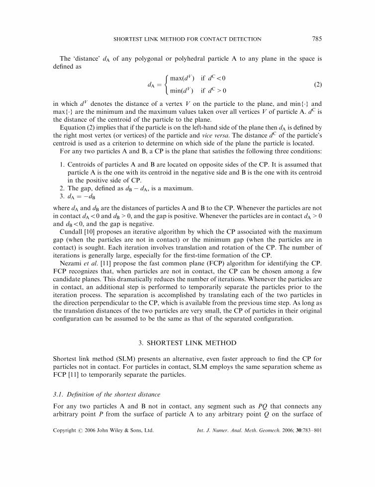
The ‘distance’ dA of any polygonal or polyhedral particle A to any plane in the space isdefined as

dA ¼maxðdV Þ if dC50

minðdV Þ if dC > 0

(ð2Þ

in which dV denotes the distance of a vertex V on the particle to the plane, and minf�g andmaxf�g are the minimum and the maximum values taken over all vertices V of particle A. dC isthe distance of the centroid of the particle to the plane.

Equation (2) implies that if the particle is on the left-hand side of the plane then dA is defined bythe right most vertex (or vertices) of the particle and vice versa. The distance dC of the particle’scentroid is used as a criterion to determine on which side of the plane the particle is located.

For any two particles A and B, a CP is the plane that satisfies the following three conditions:

1. Centroids of particles A and B are located on opposite sides of the CP. It is assumed thatparticle A is the one with its centroid in the negative side and B is the one with its centroidin the positive side of CP.

2. The gap, defined as dB � dA; is a maximum.3. dA ¼ �dB

where dA and dB are the distances of particles A and B to the CP. Whenever the particles are notin contact dA50 and dB > 0; and the gap is positive. Whenever the particles are in contact dA > 0and dB50; and the gap is negative.

Cundall [10] proposes an iterative algorithm by which the CP associated with the maximumgap (when the particles are not in contact) or the minimum gap (when the particles are incontact) is sought. Each iteration involves translation and rotation of the CP. The number ofiterations is generally large, especially for the first-time formation of the CP.

Nezami et al. [11] propose the fast common plane (FCP) algorithm for identifying the CP.FCP recognizes that, when particles are not in contact, the CP can be chosen among a fewcandidate planes. This dramatically reduces the number of iterations. Whenever the particles arein contact, an additional step is performed to temporarily separate the particles prior to theiteration process. The separation is accomplished by translating each of the two particles inthe direction perpendicular to the CP, which is available from the previous time step. As long asthe translation distances of the two particles are very small, the CP of particles in their originalconfiguration can be assumed to be the same as that of the separated configuration.

3. SHORTEST LINK METHOD

Shortest link method (SLM) presents an alternative, even faster approach to find the CP forparticles not in contact. For particles in contact, SLM employs the same separation scheme asFCP [11] to temporarily separate the particles.

3.1. Definition of the shortest distance

For any two particles A and B not in contact, any segment such as PQ that connects anyarbitrary point P from the surface of particle A to any arbitrary point Q on the surface of


SHORTEST LINK METHOD FOR CONTACT DETECTION 785

particle B is called a ‘link’ between the two particles (Figure 2). The link with the shortest lengthjPQj ¼ L is called the ‘shortest link’.

3.2. Closest points

Let A be a particle which is not in contact with the CP. Any point P on particle A for whichjdAj ¼ jdPj is called the ‘closest point’ of particle A to the CP. Figure 3 also shows the set SA;which is defined as the projections of all the closest points on the CP. Note that the set SA maycorrespond to a single vertex (Figure 3(a)), all the points on one edge (Figure 3(b)), or all thepoints on one face of the particle (Figure 3(c)).

3.3. Relationship between the shortest link and the CP

StatementThe perpendicular bisector plane (PBP) of the shortest link between two particles is the CP.

ProofLet SA and SB denote the sets of the projections of all the closest points from the particles A andB on the CP, respectively (Figure 4). The following provides a stepwise proof for the statementabove.

(i) SA \ SB=f: In other words, there is at least one point on the CP which belongs to bothsets SA and SB:

Assume that SA and SB have no overlap (Figure 4(a)). Then a line l can be drawn on the CPsuch that SA and SB are located on opposite sides of l: Rotation of the CP around the axis l inthe direction shown in Figure 4(a) will increase the distance of all the points of both particles tothe CP and results in a larger gap between the particles. This contradicts condition 2 that the CPresults in the maximum possible gap between the two particles.

Therefore, the two sets SA and SB have at least one point, such as R; in common. Point R isthe projection on CP of a closest point P from particle A, and a closest point, such as Q; onparticle B (Figure 4(b)).

(ii) The link PQ is the shortest link between the two particles.

Particle B

Particle A P

P

Q

Q

Figure 2. A link is a line segment that connects any point, P; on surface of particle A toany point, Q; on surface of particle B.



CP

A

SA

closestpoint

CP

A

SA

closestpoints

CP

A

SAclosestpoints

(a) (b)

(c)

Figure 3. Closest points of particle A to the CP and the set SA: (a) SA consists of onlyone point; (b) SA consists of all the points of a segment line; and (c) SA consists of all the

points inside and on the edges of a polygon.

CP

A

B

SA

SB

l

CP

A

SAR

P

SB

Q

B

(a) (b)

Figure 4. Relative position of SA and SB: (a) if SA \ SB ¼ f; then any rotation along lincreases the gap; and (b) R 2 SA \ SB:



Let P1Q1 be any arbitrary link with P1 on particle A and Q1 on particle B (Figure 5) and R1

be the point of intersection of segment P1Q1 and the CP. Let P01 and Q01 denote the projectionsof P1 and Q1 on the CP, respectively. As P is one of the closest points of particle A to the CP,jPRj4jP1P

01j: For the same reason, jQRj4jQ1Q

01j: So,

jP1Q1j ¼ jP1R1j þ jQ1R1j5jP1P01j þ jQ1Q

01j5jPRj þ jQRj ¼ jPQj

or

jP1Q1j5jPQj

Therefore, the link PQ is the shortest link between the two particles.(iii) The CP is the PBP of the shortest distance PQ:Point R is the projection of points P and Q on the CP. By definition, PR and QR are

perpendicular to the CP.Therefore, PQ is perpendicular to the CP.Also,

jPRj ¼ �dA and jQRj ¼ dB

From condition 3 of the definition of the CP,

�dA ¼ dB ) jPRj ¼ jQRj

Therefore, CP is the bisector of segment PQ: &

Therefore, the CP is PBP of segment PQ:

3.4. Identifying the shortest link between a point and a particle

The shortest link between a point and a particle is defined as the shortest possible segment thatconnects that point to any point from the particle. SLM frequently uses the shortest linkbetween a point in space and a particle to find the CP. This section is solely devoted to describehow such a link is found in SLM.

Let Q be a point outside particle A, as shown in Figure 6(a). Find a destination point P on thesurface of A such that PQ has the shortest possible length. Starting from any arbitrary point P0

on the surface of A, SLM obtains a series of intermediate points Pi ði ¼ 1; 2; . . . ; nÞ on thesurface of A, with jPiQj5jPi�1Qj: The last point Pn ¼ P is the closest point to Q:

Pi is determined based on the location of Pi�1 on the particle and its relative position withrespect to Q:

A B

P1

P

Q1

Q R

R1

Q´1

P´1

CP

Figure 5. PQ is the shortest link between the two particles.



Case 1: Pi�1 is a vertex of particle A (Figure 6(b)). In this case Pi is sought only on theneighbouring faces of Pi�1 (neighbouring faces of a vertex are those that share that vertex).

Case 2: Pi�1 is located on an edge of the particle but not on the vertices connected to it(Figure 6(c)). In this case point Pi is sought only on the two neighbouring faces that share thatedge.

Case 3: Pi�1 is located on a face of the particle but not on any edges or vertices of that face,Figure 6(d). In this case point Pi is sought only on the same face (including its edges andvertices).

The process continues until Pi ¼ Pi�1: The number of iterations depends on the relativeposition of the starting point P0 and point Q; as well as the geometry of the particle. The closerthe starting point P0 to destination point P; the faster the algorithm converges and less numberof iterations required.

3.5. CP identification in SLM

SLM indirectly identifies the CP by seeking the shortest link between the two particles.The algorithm seeks two points P 2 A and P 2 B such that PQ is the shortest link betweenparticles A and B. Starting from any two arbitrary points P0 2 A and Q0 2 B; SLM usesan iterative process, in which a series of intermediate points Pi 2 A and Qi 2 B ði ¼ 1; . . . ; nÞare found, such that Pn ¼ P and Qn ¼ Q (Figure 7). The ith iteration consists of two stepsas follows.

Step 1. For the point Qi�1; use the algorithm in Section 3.4 to find the closest point Pi onparticle A. Use Pi�1 as the starting point on particle A.

Particle A

Pi-1

Particle A

Pi-1

Particle A

Pi-1

Q

Particle A

P2P1

P0

P3 = P

(a) (b)

(c) (d)

Figure 6. Shortest link between a point and a particle: (a) SLM iterative process to find point P from P0;(b) Pi�1 is a vertex of particle A; (c) Pi�1 is on an edge; and (d) Pi�1 is on a face.



Step 2. For the newly found point Pi; use the same algorithm to find the closest point Qi onparticle B. Use Qi�1 as the starting point.

The ith iteration results in a pair of ðPi;QiÞ such that jPi�1Qi�1j > jPiQi j: The iterativeprocess continues until Pi ¼ Pi�1 and Qi ¼ Qi�1: The number of iterations depends on thestarting points P0Q0 as well as relative displacement of particles from the previous time step.In DEM applications, the change in particles’ positions between two time steps is very small.As a result, the average number of iterations required in SLM is rarely larger than 3 (seeSection 5).

3.5.1. Initialization. The first iteration for finding the shortest link requires two startingpoints P0 and Q0 on the surface of particles. If a shortest link is available from theprevious DEM time step, then the endpoints of that link are used as P0 and Q0: If there isno shortest link available from the previous DEM time step (that is, no CP has been detectedso far between the two particles), then three steps are performed to obtain the starting pointsP0 and Q0:

1. The PBP of the line that connects the centroids of the two particles is drawn.2. Among all the vertices of particle A, the one with the minimum absolute distance from that

plane is chosen as P0:3. Among all the vertices of particle B, the one with the minimum absolute distance from that

plane is chosen as Q0:

3.5.2. Special cases for identifying the shortest link. There are a few cases in which the SLMiterative scheme results in large number of iterations or potentially an infinite loop. One possibleexample is shown in Figure 8(a), in which both points P 0 and Q 0 are located on edges ofparticles. Applying the iterative SLM process results in a series of points Pi and Qi; all remainingon the same two edges. Such large/infinite loops may occur only if both points P 0 and Q 0 arelocated on faces or edges of particles and are limited to those shown in Figure 8(a–c). In Figure8(b) both points P0 and Q0 are located on faces of particles, and in Figure 8(c) one point is on anedge and the other one is on a face.

The above iterative algorithm is modified to prevent any potential large/infinite loop. At thebeginning of each iteration step, points Pi�1 and Qi�1 are examined. If they fall in one of the

Particle BParticle A

QQn =

1i−P

PP n =

1−iQ

0P

0Q

Figure 7. Shortest link method algorithm.



following three categories, then, instead of SLM iterative scheme, a direct geometrical approachis used to find the points Pi and Qi:

Case 1: If Pi�1 and Qi�1 are both located on edges (but not vertices) of particles, then pointsPi and Qi are found on the same edges, such that segment jPiQij has the shortest possible lengthbetween the two edges. This is done in three steps as follows:

i. Let e1 and e2 denote the edges. Let P be a plane parallel to both e1 and e2: Theprojections AB and CD of the two edges on plane P are obtained (Figure 9).

ii. Points P0 2 AB and Q0 2 CD are found such that P0Q0 is the shortest link betweensegments AB and CD (see Appendix A for details).

iii. The points Pi 2 e1 and Qi 2 e2 corresponding to P0 and Q0 are determined.

Case 2: If both Pi�1 and Qi�1 are located on the faces of particles (but not edges or vertices),then the following steps are performed:

i. Let f1 and f2 denote the planes containing the faces (Figure 10). Let P be the planenormal to both f1 and f2 that passes through Pi�1: The intersections of P and the facesdefine two line segments (AB and CD in Figure 10).

ii. The endpoints of the shortest link between the two segments AB and CD (found asexplained in Appendix A) define Pi and Qi:

Case 3: If one of Pi�1 or Qi�1 is located on an edge (not a face or a vertex) and the other oneon a face (not an edge or a vertex), then the following steps are performed to find Pi and Qi:

i. Let P denote the plane passing through the edge (e1 in Figure 11) normal to the face (f1).Such a plane specifies a line segment AB on the face.

ii. The endpoints of the shortest link between the edge and the segment AB (obtained asexplained in Appendix A) define Pi and Qi:

P0

Q0

Q1

P1

Particle A

Particle B

Q2

P2

Q3

(a)

P0

Q0

Q1

Q3

P1P2

Q2

Particle B

Particle A

(b)

P0

Q0

Q1

Q3

P1P2

Q2

Particle B

Particle A

(c)

Figure 8. Cases with non-unique shortest link: (a) both points are on edges; (b) both points are on faces;and (c) one point is on a face and the other on an edge.



Π

A

B

DC = Q´

P´

iP

iQ

e2e1

Figure 9. P0Q0 is the shortest link between segments AB and CD: Pi is the point corresponding toP0: Qi is the point corresponding to Q0:

A B

C = iQ

D

f2

f1

Π Π

iP

Figure 10. P is the plane normal to both faces. The shortest link betweensegments AB and CD defines PiQi:

A B

iQΠ Π

iPf1

e1

Figure 11. P is the plane normal to the face passing through the edge. The shortest link betweensegment AB and edge e1 defines PiQi:



3.6. 2-D implementation of SLM

In 2-D, the CP is a line rather than a plane. However, definitions of the shortest link and theshortest distance as well as the statement of Section 3.3 still hold. The algorithm to obtain theshortest link between a point and a particle in Section 3.4 is simplified as follows:

Case 1: Pi�1 is a vertex of particle A. In this case Pi is sought only on the two edges that share Pi�1:Case 2: Pi�1 is located on an edge of the particle but not on any vertices of that edge. In this

case point Pi is sought only on the same edge (including its vertices).In 2-D, CP identification algorithm of Section 3.5 is as follows. Starting from initial points

P0 2 A and Q0 2 B; a series of intermediate points Pi 2 A and Qi 2 B ði ¼ 1; . . . ; nÞ are found, inwhich the ith iteration consists of the two following steps.

Step 1: For the point Qi�1; find the closest point Pi on particle A.Step 2: For the newly found point Pi; find the closest point Qi on particle B.In the beginning of each iteration, if Pi�1 and Qi�1 are both located on edges of particles then,

instead of the iterative process explained above, points Pi and Qi are found on the same edges,such that segment jPiQij has the shortest possible length between the two edges.

4. UNIQUENESS OF CP

StatementFor any two convex particles the CP defined in Section 2.1 is unique.

ProofAssume that for two convex particles A and B, two different CPs exist, both satisfyingconditions 1–3 of the definition of the CP, and each of them being the PBP of a shortest linkbetween the two particles. Let PQ and P0Q0 be the associated shortest links, where P and P0

belong to particle A, and Q and Q0 belong to particle B (Figure 12).The following proves that the PBP of these two shortest link are identical.(i) P1Q1Q2P2 is a parallelogramAny point p ¼ ðp1; p2; p3Þ on segment PP0 (with pi being the ith Cartesian component in the

global Cartesian co-ordinate system 1-2-3) can be described as

pi ¼ Pi þmir; 04r41; i ¼ 1; 2; 3 ð3aÞ

where P ¼ ðP1;P2;P3Þ and subscript i represents the ith Cartesian component.

Particle A Particle B

P

P´

Q

Q´

H

Figure 12. Uniqueness of the CP.



!m ¼ ðm1;m2;m3Þ is the vector pointing from P to P0:

mi ¼ Pi � P0i; i ¼ 1; 2; 3

Likewise, any point q ¼ ðq1; q2; q3Þ on segment QQ0 can be represented as

qi ¼ Qi þ nis; 04s41; i ¼ 1; 2; 3 ð3bÞ

where Q ¼ ðQ1;Q2;Q3Þ and ni ¼ Qi �Q0i; i ¼ 1; 2; 3:The distance from a point p on PP0 to a point q on segment QQ0 is a function of two variables

r and s and is given by

Lðr; sÞ ¼

ffiffiffiffiffiffiffiffiffiffiffiffiffiffiffiffiffiffiffiffiffiffiffiffiffiffiffiffiffiffiffiffiX3

i¼1ðpi � qiÞ

2

r; 04r; s41 ð4Þ

Substituting from (3a) in (4) results in

Lðr; sÞ ¼

ffiffiffiffiffiffiffiffiffiffiffiffiffiffiffiffiffiffiffiffiffiffiffiffiffiffiffiffiffiffiffiffiffiffiffiffiffiffiffiffiffiffiffiffiffiffiffiffiffiffiffiffiffiffiffiffiffiffiX3

i¼1ðPi �Qi þmir� nisÞ

2

r; 04r; s41 ð5Þ

Note that

jPQj ¼ Lð0; 0Þ ¼

ffiffiffiffiffiffiffiffiffiffiffiffiffiffiffiffiffiffiffiffiffiffiffiffiffiffiffiffiffiffiffiffiffiX3

i¼1ðPi �QÞ2

r¼ L ð6aÞ

and

jP0Q0j ¼ Lð1; 1Þ ¼

ffiffiffiffiffiffiffiffiffiffiffiffiffiffiffiffiffiffiffiffiffiffiffiffiffiffiffiffiffiffiffiffiffiffiffiffiffiffiffiffiffiffiffiffiffiffiffiffiffiffiffiffiffiX3

i¼1ðPi �Qþmi � niÞ

2

r¼ L ð6bÞ

Combining (6a) and (6b) ffiffiffiffiffiffiffiffiffiffiffiffiffiffiffiffiffiffiffiffiffiffiffiffiffiffiffiffiffiffiffiffiffiX3

i¼1ðPi �QÞ2

r¼

ffiffiffiffiffiffiffiffiffiffiffiffiffiffiffiffiffiffiffiffiffiffiffiffiffiffiffiffiffiffiffiffiffiffiffiffiffiffiffiffiffiffiffiffiffiffiffiffiffiffiffiffiffiX3

i¼1ðPi �Qþmi � niÞ

2

r

or

2X3i¼1

ðPi �QiÞðmi � niÞ ¼ �X3i¼1

ðmi � niÞ2 ð7Þ

Convexity of particles guarantees that any point on segments PP0 and QQ0 is located inside oron the surface of particles A and B, respectively. As a result, the distance between any point p onPP0 and any point q on QQ0 is greater than the shortest distance L:

Lðr; sÞ5L; 04r; s41

or

Lðr; sÞ2 � L250; 04r; s41 ð8Þ

Substituting (5) in (8)X3i¼0

ðPi �Qi þmir� nisÞ2 � ðPi �QiÞ

250; 04r; s41

or X3i¼0

2ðPi �QiÞðmir� nisÞ þX3i¼0

ðmir� nisÞ250; 04r; s41



For ðr ¼ sÞ

2rX3i¼0

ðPi �QiÞðmi � niÞ þ r2X3i¼0

ðmi � niÞ250; 04r41 ð9Þ

Substituting (7) in (9) gives

�rX3i¼0

ðmi � niÞ2 þ r2

X3i¼0

ðmi � niÞ250; 04r41

or

ðr2 � rÞX3i¼0

ðmi � niÞ250; 04r41 ð10Þ

On the other hand,P3

i¼0 ðmi � niÞ2 is always zero or positive and for any 05r51; ðr2 � rÞ is

negative; that is,

ðr2 � rÞX3i¼0

ðmi � niÞ240; 04r41 ð11Þ

Combining (10) and (11) results in

ðr2 � rÞX3i¼0

ðmi � niÞ2 ¼ 0; 04r41

or

X3i¼0

ðmi � niÞ2 ¼ 0

which leads to

mi ¼ ni; i ¼ 1; 2; 3 ð12Þ

This proves that PQ ¼ P0Q0 and PQjjP0Q0:Therefore, P1Q1Q2P2 is a parallelogram.(ii) P1Q1Q2P2 is a rectangleIf PP0 is not perpendicular to PQ (Figure 12), then a point such as H can be found on QQ0;

such that jPH j5jPQj; which is a contradiction. As a result, P1P2 ? P1Q1:Therefore, P1Q1Q2P2 is a rectangle.(iii) CP is uniqueFrom (ii) PBP’s of P1Q1 and P2Q2 are identical.Therefore, the two CPs are identical. &

5. IMPLEMENTATION AND EXAMPLES

The performance of the SLM algorithm is demonstrated through a series of examples for 2-Dand 3-D particles. The computation time is compared with that using the FCP algorithmproposed by Nezami et al. [11] and the original iterative algorithm used by Cundall [10].



5.1. Contact detection in 2-D

Figure 13 depicts nine pairs of particles in various configurations in 2-D. For each config-uration, no previous CP is available. The CPs are obtained with both SLM, FCP and theconventional CP method and are shown in the figure, along with the shortest link for eachconfiguration. The resulting CPs from all three algorithms are identical. The speed up ratio R;defined as the ratio of the CPU run time for the conventional algorithm to that for SLMor FCP, is shown for each configuration and varies from 5 to 16 for SLM compared to 1–5for FCP.

SLM: R=5.7

FCP: R=2.3

SLM: R=9.6

FCP: R=3.1

SLM: R=16.4

FCP: R=4.6

SLM: R=5.0

FCP: R=2.6

SLM: R=11.3

FCP: R=3.3

SLM: R=11.8

FCP: R=3.0

SLM: R=15.9

FCP: R=3.6

SLM: R=9.8

FCP: R=1.3

SLM: R=10.5

FCP: R=3.7

Figure 13. SLM performance in 2-D relative to iterative method.



5.2. Contact detection in 3-D

SLM algorithm is implemented in the 3-D computer program BLOCKS3D version 2.0,developed by the authors. The program simulates polyhedral particles of any shape and sizedistribution. The performance of SLM is demonstrated through a series of examples andcompared to FCP and conventional common plane method [10] and FCP [11].

5.2.1. Simulation of particle flow. This set of examples consists of ten simulations. For eachsimulation a number of particles are dropped into a cubic box. For the first two simulations(500 and 4000 particles) a 0:30 m� 0:30 m box is used while the other eight simulations aredone using a 1:0 m� 1:0 m box. The average particle size in all simulations is D50 ¼ 3:8 cm;with minimum and maximum particle sizes of 2.0 and 5:0 cm; respectively. The time step is1:3� 10�4 s: The particles’ geometries are chosen evenly from those shown in Figure 14, andhave the following contact properties:

Normal stiffness Kn: 130 KN=mShear stiffness Ks: 102 KN=mContact friction angle fm: 358

Small stiffness values are chosen deliberately to increase the time step and reduce thecomputational effort. Once the particles are accumulated inside the box, two adjacent walls ofthe box are removed, allowing the particles to flow in two directions.

Figure 15 plots three snapshots of the simulation for 45 000 particles. The test is continueduntil the final stable configuration is achieved.

Figure 14. Particles with 4 vertices (tetrahedron), 5 vertices (pyramid), 8 vertices (cube) and 14 vertices.

Figure 15. Particle flow: simulation with 45 000 particles: (a) t ¼ 0:0 s; (b) t ¼ 1:4 s; and (c) t ¼ 2:0 s:



For each simulation, the speed up ratio R (defined as the ratio of the CPU run time spent inthe CP detection subroutines for conventional CP method to that for the FCP and SLM) isevaluated during the first 1000 time steps of the flow phase and is shown in Figure 16 as afunction of number of particles. The speed up ratio ranges for FCP algorithm from 13 to 10 andfor SLM algorithm from 21 to 17. The speed up ratio decreases with increasing number ofparticles; but, nevertheless, SLM provides consistently significant speed up. For SLMsimulations, the number of iterations required to calculate the CP at each time step is recorded.It is observed that around 95% of the contacts require two or less iterations in SLM.

5.2.2. Simulation of soil–tool interaction. This simulation involves pushing a loader bucket intoa pile of soil and lifting a load. The soil pile is generated by dropping 21 952 particles into a soilbin, composed of two side plates 0.60m apart and two end plates 0.4m apart. Then one of theend walls is removed allowing the particles to flow along the bin. The particles geometries arechosen evenly from those shown in Figure 14, with an average particle size of D50 ¼ 2:5 cm withminimum and maximum particle sizes of 1.0 and 4:0 cm; respectively. Contact properties of theparticles are the same as those in the prior simulations. Time step is chosen to be 1:2� 10�4 s:

The bucket is a scaled, simplified prototype of a typical commercial loader bucket, modelledwith five plates, as shown in Figure 17. It is initially positioned at an elevation 0:04 m above theground. The displacement of the bucket consists of a horizontal translation phase in which the

8

10

12

14

16

18

20

22

0 10,000 20,000 30,000 40,000 50,000

Shortest link methodFast common plane method

Spee

d up

rat

io, R

Number of particles

Figure 16. Speed up ratio R of SLM and FCP methods compared to conventional CP method.



bucket is pushed into the soil pile, a rotational phase, and a vertical translation phase. Eachphase is performed at a constant velocity.

Table I shows the duration of each phase along with the corresponding total displacement orrotation of the bucket. Figure 18 plots the initial configuration and a cross section of the pile(passing through the centreline of the bucket) at three different time steps.

The speed up ratio of both SLM and FCP compared to the conventional CP method arecalculated for the first 1000 time steps of each phase of bucket motion and shown in Table I. Aspeed up ratio of about 18 is observed for SLM and 12 for FCP. More than 98% of the contactsrequire two or less iterations in SLM.

6. CONCLUSION

It is shown that the common plane can be uniquely defined as the perpendicular bisector planeof the shortest link between the two particles. Based on this observation, a new algorithmis proposed in which the shortest link is sought. The algorithm is developed for convex 2-D and3-D polyhedral particles.

The performance of the new algorithm is examined through several examples. It is observedthat for large number of particles, the current algorithm runs up to 17 times faster thanconventional common plane.

Figure 17. Loader bucket, simulated by five plates.

Table I. Soil–tool interaction, speed up of SLM and FCP relative to iterative CP procedure.

Speed up ratio

Displacement phase Displacement Start time (s) End time (s) SLM FCP

Horizontal translation 0:25 m 0 8 18.31 12.54Rotation 658 5 16 18.14 11.12Vertical translation 0:18 m 13 20 18.05 11.68



APPENDIX A

This section provides an algorithm to obtain the shortest link between any two co-planar linesegments. The algorithm is frequently used in SLM scheme (Section 3.5.2). Let AB and CDdenote two co-planar segments as shown in Figure A1.

If AB and CD intersect, then the intersection point is the shortest link. In this case the shortestlink has a length of zero and is reduced to a point, Figure 19(a).

If AB and CD do not intersect, then the shortest link is the shortest segment among thefollowing, Figure A1(b).

i. AC, BC, AD, CD (Figure A1(b), left).ii. AA1; BB1; CC1 and DD1 where A1 and B1 are the projection of A and B on CD and C1

and D1 are the projections of C and D on AB (Figure A1(b), right). Note that among AA1;BB1; CC1 and DD1; only those with both ends inside the line segments are considered.

Figure 18. Soil–tool interaction simulation: (a) Initial configuration; (b) t ¼ 0:0 s;(c) t ¼ 5:0 s; and (d) t ¼ 20:0 s:

A

B

D

C A

D

C

B1

C1

A1

B D1A B

D

C

(a) (b)

Figure A1. The shortest link between two co-planar segments AB and CD: (a) AB and CD intersect;and (b) AB and CD do not intersect; CC1 is the shortest link.



ACKNOWLEDGEMENTS

This material is based upon work supported by the National Science Foundation under Grant No. CMS-0113745 and Caterpillar, Inc. Any opinions, findings, and conclusions or recommendations expressed inthis material are those of the authors and do not necessarily reflect the views of the National ScienceFoundation or Caterpillar, Inc. This support is gratefully acknowledged. The authors would also like tothank Mr Ibrahim Mohammad for preparing the visualization code VisDEM3D.

REFERENCES

1. Cundall PA. A computer model for simulating progressive large-scale movements in block rock mechanics.Proceedings of the Symposium of International Society of Rock Mechanics, vol. 8. Nancy, 1971.

2. Cundall PA, Strack ODL. A discrete numerical model for granular assemblies. Geotechnique 1979; 29(1):47–65.3. Bardet JP. Numerical simulation of the incremental responses of idealized granular materials. International Journal

of Plasticity 1994; 10(8):879–908.4. Thornton C, Barnes DJ. Computer simulated deformation of compact granular assemblies. Acta Mechanica 1986;

64:45–61.5. Bagi K. Stress and strain in granular assemblies. Mechanics of Materials 1996; 22:165–177.6. Cleary PW, Campbell CS. Self-lubrication for long run-out landslides: examination by computer simulation. Journal

of Geophysical Research}Solid Earth 1993; 98(B12):21911–21924.7. Campbell CS, Cleary PW, Hopkins MA. Large-scale landslide simulations: global deformation, velocities, and basal

friction. Journal of Geophysical Research}Solid Earth 1995; 100(B5):8267–8283.8. Hopkins MA, Hibler WD, Flato GM. On the numerical simulation of the sea ice ridging process. Journal of

Geophysical Research}Oceans 1991; 96(C3):4809–4820.9. Cleary PW. DEM simulation of industrial particle flows: case studies of dragline excavators, mixing in tumblers and

centrifugal mills. Powder Technology 2000; 209(1–3):83–104.10. Cundall PA. Formulation of a three-dimensional distinct element model. Part I: a scheme to detect and represent

contacts in a system composed of many polyhedral blocks. International Journal of Rock Mechanics, and MiningSciences & Geomechanics Abstracts 1988; 25(3):107–116.

11. Nezami E, Hashash YMA, Zhao D, Ghaboussi J et al. A fast contact detection algorithm for 3-D discrete elementmethod. Computers and Geotechnics 2004; 31(7):575–587.



Shortest link method for contact detection in discrete element method

Documents

Transcript of Shortest link method for contact detection in discrete element method