Nonlinear Analysis 74 (2011) 7365–7379

Contents lists available at SciVerse ScienceDirect

Nonlinear Analysis

journal homepage: www.elsevier.com/locate/na

Higher-order radial derivatives and optimality conditions in nonsmoothvector optimizationNguyen Le Hoang Anh a, Phan Quoc Khanh b, Le Thanh Tung c,∗

a Department of Mathematics, University of Science of Hochiminh City, 227 Nguyen Van Cu, District 5, Hochiminh City, Viet Namb Department of Mathematics, International University of Hochiminh City, Linh Trung, Thu Duc, Hochiminh City, Viet Namc Department of Mathematics, College of Science, Cantho University, Ninhkieu District, Cantho City, Viet Nam

a r t i c l e i n f o

Article history:Received 18 February 2011Accepted 27 July 2011Communicated by Ravi Agarwal

MSC:90C4649J5246G0590C2690C29

Keywords:Higher-order outer and inner radialderivatives

Calculus rulesQ -minimalityIdeal and weak efficiencyVarious kinds of proper efficiencyHigher-order optimality conditionsSet-valued vector optimization

a b s t r a c t

We propose notions of higher-order outer and inner radial derivatives of set-valued mapsandobtainmain calculus rules. Somedirect applications of these rules in proving optimalityconditions for particular optimization problems are provided. Then we establish higher-order optimality necessary conditions and sufficient ones for a general set-valued vectoroptimizationproblemwith inequality constraints. A number of examples illustrate both thecalculus rules and the optimality conditions. In particular, they explain some advantagesof our results over earlier existing ones and why we need higher-order radial derivatives.

© 2011 Elsevier Ltd. All rights reserved.

1. Introduction and preliminaries

In nonsmooth optimization, a large number of generalized derivatives have been introduced to replace the classicalFréchet andGateaux derivatives tomeet the continually increasing diversity of practical problems.We can recognize roughlytwo approaches: primal space and dual space approaches. Coderivatives, limiting subdifferentials and other notions in thedual space approach enjoy rich and fruitful calculus rules and little depend on convexity assumptions in applications; seee.g. the excellent book [1,2]. The primal space approach has beenmore developed so far, partially since it ismore natural andexhibits clear geometrical interpretations. Most generalized derivatives in this approach are based on linear approximationsand kinds of tangency. Hence, approximating cones play crucial roles. One of the early and most important notions are thecontingent cone and the corresponding contingent derivative; see [3,4]. For a subset A of a normed space X , the contingentcone of A at x ∈ cl A is

TA(x) = {u ∈ X : ∃tn → 0+, ∃un → u, ∀n, x + tnun ∈ A}.

∗ Corresponding author. Tel.: +84 909353482.E-mail addresses: nlhanh@hcmuns.edu.vn (N.L.H. Anh), pqkhanh@hcmiu.edu.vn (P.Q. Khanh), lttung@ctu.edu.vn, lttungct@gmail.com (L.T. Tung).

0362-546X/$ – see front matter© 2011 Elsevier Ltd. All rights reserved.doi:10.1016/j.na.2011.07.055

7366 N.L.H. Anh et al. / Nonlinear Analysis 74 (2011) 7365–7379

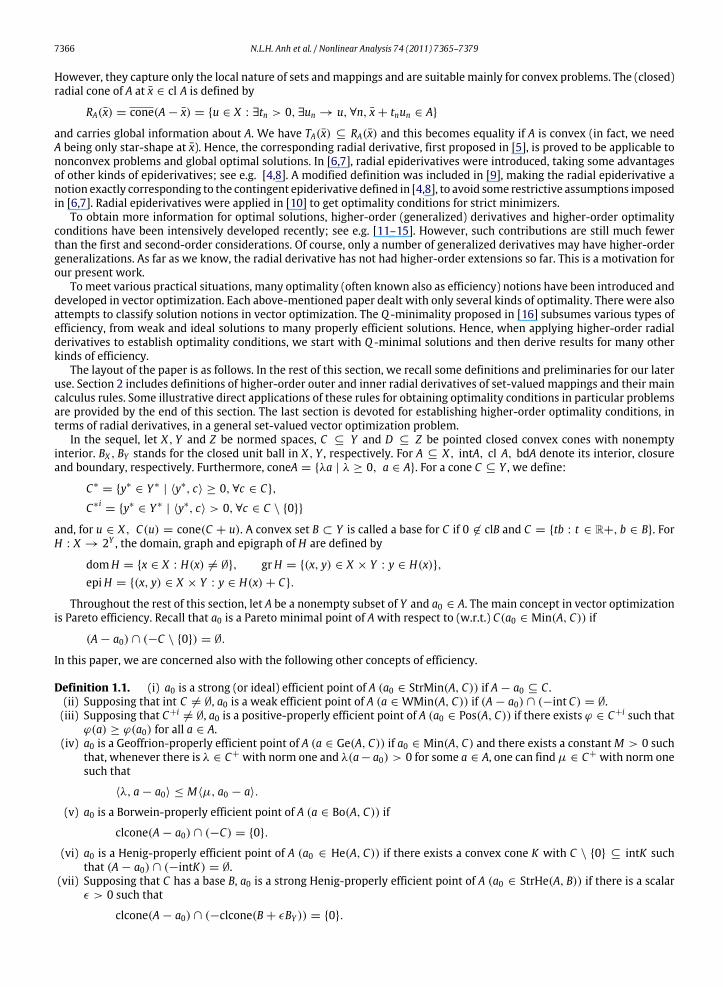
However, they capture only the local nature of sets andmappings and are suitable mainly for convex problems. The (closed)radial cone of A at x ∈ cl A is defined by

RA(x) = cone(A − x) = {u ∈ X : ∃tn > 0, ∃un → u, ∀n, x + tnun ∈ A}

and carries global information about A. We have TA(x) ⊆ RA(x) and this becomes equality if A is convex (in fact, we needA being only star-shape at x). Hence, the corresponding radial derivative, first proposed in [5], is proved to be applicable tononconvex problems and global optimal solutions. In [6,7], radial epiderivatives were introduced, taking some advantagesof other kinds of epiderivatives; see e.g. [4,8]. A modified definition was included in [9], making the radial epiderivative anotion exactly corresponding to the contingent epiderivative defined in [4,8], to avoid some restrictive assumptions imposedin [6,7]. Radial epiderivatives were applied in [10] to get optimality conditions for strict minimizers.

To obtain more information for optimal solutions, higher-order (generalized) derivatives and higher-order optimalityconditions have been intensively developed recently; see e.g. [11–15]. However, such contributions are still much fewerthan the first and second-order considerations. Of course, only a number of generalized derivatives may have higher-ordergeneralizations. As far as we know, the radial derivative has not had higher-order extensions so far. This is a motivation forour present work.

To meet various practical situations, many optimality (often known also as efficiency) notions have been introduced anddeveloped in vector optimization. Each above-mentioned paper dealt with only several kinds of optimality. There were alsoattempts to classify solution notions in vector optimization. The Q -minimality proposed in [16] subsumes various types ofefficiency, from weak and ideal solutions to many properly efficient solutions. Hence, when applying higher-order radialderivatives to establish optimality conditions, we start with Q -minimal solutions and then derive results for many otherkinds of efficiency.

The layout of the paper is as follows. In the rest of this section, we recall some definitions and preliminaries for our lateruse. Section 2 includes definitions of higher-order outer and inner radial derivatives of set-valued mappings and their maincalculus rules. Some illustrative direct applications of these rules for obtaining optimality conditions in particular problemsare provided by the end of this section. The last section is devoted for establishing higher-order optimality conditions, interms of radial derivatives, in a general set-valued vector optimization problem.

In the sequel, let X, Y and Z be normed spaces, C ⊆ Y and D ⊆ Z be pointed closed convex cones with nonemptyinterior. BX , BY stands for the closed unit ball in X, Y , respectively. For A ⊆ X, intA, cl A, bdA denote its interior, closureand boundary, respectively. Furthermore, coneA = {λa | λ ≥ 0, a ∈ A}. For a cone C ⊆ Y , we define:

C∗= {y∗

∈ Y ∗| ⟨y∗, c⟩ ≥ 0, ∀c ∈ C},

C∗ i= {y∗

∈ Y ∗| ⟨y∗, c⟩ > 0, ∀c ∈ C \ {0}}

and, for u ∈ X, C(u) = cone(C + u). A convex set B ⊂ Y is called a base for C if 0 ∈ clB and C = {tb : t ∈ R+, b ∈ B}. ForH : X → 2Y , the domain, graph and epigraph of H are defined by

domH = {x ∈ X : H(x) = ∅}, grH = {(x, y) ∈ X × Y : y ∈ H(x)},epiH = {(x, y) ∈ X × Y : y ∈ H(x) + C}.

Throughout the rest of this section, let A be a nonempty subset of Y and a0 ∈ A. The main concept in vector optimizationis Pareto efficiency. Recall that a0 is a Pareto minimal point of A with respect to (w.r.t.) C(a0 ∈ Min(A, C)) if

(A − a0) ∩ (−C \ {0}) = ∅.

In this paper, we are concerned also with the following other concepts of efficiency.

Definition 1.1. (i) a0 is a strong (or ideal) efficient point of A (a0 ∈ StrMin(A, C)) if A − a0 ⊆ C .(ii) Supposing that int C = ∅, a0 is a weak efficient point of A (a ∈ WMin(A, C)) if (A − a0) ∩ (−int C) = ∅.(iii) Supposing that C+i

= ∅, a0 is a positive-properly efficient point of A (a0 ∈ Pos(A, C)) if there exists ϕ ∈ C+i such thatϕ(a) ≥ ϕ(a0) for all a ∈ A.

(iv) a0 is a Geoffrion-properly efficient point of A (a ∈ Ge(A, C)) if a0 ∈ Min(A, C) and there exists a constantM > 0 suchthat, whenever there is λ ∈ C+ with norm one and λ(a− a0) > 0 for some a ∈ A, one can find µ ∈ C+ with norm onesuch that

⟨λ, a − a0⟩ ≤ M⟨µ, a0 − a⟩.

(v) a0 is a Borwein-properly efficient point of A (a ∈ Bo(A, C)) if

clcone(A − a0) ∩ (−C) = {0}.

(vi) a0 is a Henig-properly efficient point of A (a0 ∈ He(A, C)) if there exists a convex cone K with C \ {0} ⊆ intK suchthat (A − a0) ∩ (−intK) = ∅.

(vii) Supposing that C has a base B, a0 is a strong Henig-properly efficient point of A (a0 ∈ StrHe(A, B)) if there is a scalarϵ > 0 such that

clcone(A − a0) ∩ (−clcone(B + ϵBY )) = {0}.

N.L.H. Anh et al. / Nonlinear Analysis 74 (2011) 7365–7379 7367

(viii) a0 is a super efficient point of A (a0 ∈ Su(A, C)) if there is a scalar ρ > 0 such that

clcone(A − a0) ∩ (BY − C) ⊆ ρBY .

Note that Geoffrion originally defined the properness notion in (iv) for Rn with the ordering cone Rn+. Hartley extended

it to the case of arbitrary convex ordering cone. The above general definition of Geoffrion properness is taken from [17].For relations of the above notions and also other kinds of efficiency, see e.g. [16–20]. Some of them are collected in theproposition below.

Proposition 1.1. (i) StrMin(A) ⊆ Min(A) ⊆ WMin(A).(ii) Pos(A) ⊆ He(A) ⊆ Min(A).(iii) Su(A) ⊆ Ge(A) ⊆ Bo(A) ⊆ Min(A).(iv) Su(A) ⊆ He(A).(v) Su(A) ⊆ StrHe(A) and if C has a bounded base then Su(A) = StrHe(A).

From now on, unless otherwise specified, let Q ⊆ Y be an arbitrary nonempty open cone, different from Y .

Definition 1.2 ([16]).We say that a0 is a Q -minimal point of A (a0 ∈ Qmin(A)) if

(A − a0) ∩ (−Q ) = ∅.

Recall that an open cone in Y is said to be a dilating cone (or a dilation) of C , or dilating C if it contains C \ {0}. Let B beas before a base of C . Setting

δ = inf{‖b‖ : b ∈ B} > 0,

for each 0 < ϵ < δ, we associate to C a pointed open convex cone Cϵ(B), defined by

Cϵ(B) = cone(B + ϵBY ).

For each ϵ > 0, we also associate to C another open cone C(ϵ) defined as

C(ϵ) = {y ∈ Y : dC (y) < ϵd−C (y)}.

The various kinds of efficient points in Definition 1.1 are in fact Q -minimal points with Q being appropriately chosencones as follows.

Proposition 1.2 ([16]).

(i) a0 ∈ StrMin(A) if and only if a0 ∈ Qmin(A) with Q = Y \ (−C).(ii) a0 ∈ WMin(A) if and only if a0 ∈ Qmin(A) with Q = int C.(iii) a0 ∈ Pos(A) if and only if a0 ∈ Qmin(A) with Q = {y ∈ Y | ϕ(y) > 0}, ϕ being some functional in C+i.(iv) a0 ∈ Ge(A) if and only if a0 ∈ Qmin(A) with Q = C(ϵ) for some ϵ > 0.(v) a0 ∈ Bo(A) if and only if a0 ∈ Qmin(A) with Q being some open cone dilating C.(vi) a0 ∈ He(A) if and only if a0 ∈ Qmin(A) with Q being some open pointed convex cone dilating C.(vii) a0 ∈ StrHe(A) if and only if a0 ∈ Qmin(A) with Q = int Cϵ(B), ϵ satisfying 0 < ϵ < δ.(viii) (supposing that C has a bounded base) a0 ∈ Su(A) if and only if a0 ∈ Qmin(A)with Q = intCϵ(B), ϵ satisfying 0 < ϵ < δ.

2. Higher-order radial derivatives

We propose the following higher-order radial derivatives.

Definition 2.1. Let F : X → 2Y be a set-valued map and u ∈ X .

(i) Themth-order outer radial derivative of F at (x0, y0) ∈ gr F is

DmR F(x0, y0)(u) = {v ∈ Y : ∃tn > 0, ∃(un, vn) → (u, v), ∀n, y0 + tmn vn ∈ F(x0 + tnun)}.

(ii) Themth-order inner radial derivative of F at (x0, y0) ∈ gr F is

DmR F(x0, y0)(u) = {v ∈ Y : ∀tn > 0, ∀un → u, ∃vn → v, ∀n, y0 + tmn vn ∈ F(x0 + tnun)}.

Remark 2.1. Let us discuss some ideas behind this definition. The term ‘‘radial’’ in the definitions of the radial set orderivative of a map means taking directions which give points having global properties related to the set or graph of themap, not only local ones around the considered point (as in usual notions like the contingent derivative, where tn → 0+

appears). Here we propose higher-order notions based on this idea. Moreover, the higher-order character in our definition

7368 N.L.H. Anh et al. / Nonlinear Analysis 74 (2011) 7365–7379

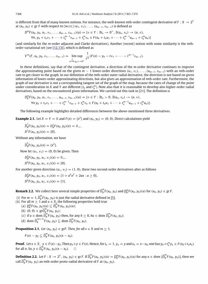
is different from that of many known notions. For instance, the well-knownmth-order contingent derivative of F : X → 2Y

at (x0, y0) ∈ gr F with respect to (w.r.t.) (u1, v1), . . . , (um−1, vm−1) is defined as

DmF(x0, y0, u1, v1, . . . , um−1, vm−1)(u) = {v ∈ Y : ∃tn → 0+, ∃(un, vn) → (u, v),

∀n, y0 + tnv1 + · · · + tm−1n vm−1 + tmn vn ∈ F(x0 + tnu1 + · · · + tm−1

n um−1 + tmn un)}

(and similarly for the m-order adjacent and Clarke derivatives). Another (recent) notion with some similarity is the mth-order variational set (see [12,13]), which is defined as

Vm(F , x0, y0, v1, . . . , vm−1) = lim supx

F−→x0,t→0+

1tm

(F(x) − y0 − tv1 − · · · − tm−1vm−1).

In these definitions, say that of the contingent derivative, a direction of the m-order derivative continues to improvethe approximating point based on the given m − 1 lower-order directions (u1, v1), . . . , (um−1, vm−1) with an mth-orderrate to get closer to the graph. In our definition of themth-order outer radial derivative, the direction is not based on giveninformation of lower-order approximating directions, but also gives an approximation of mth-order rate. Furthermore, thegraph of our derivative is not a corresponding tangent set of the graph of the map, because the rates of change of the pointunder consideration in X and Y are different (tn and tmn ). Note also that it is reasonable to develop also higher-order radialderivatives, based on the encountered given information. We carried out this task in [21]. The definition is

DmR F(x0, y0, u1, v1, . . . , um−1, vm−1)(u) = {v ∈ Y : ∃tn > 0, ∃(un, vn) → (u, v),

∀n y0 + tnv1 + · · · + tm−1n vm−1 + tmn vn ∈ F(x0 + tnu1 + · · · + tm−1

n um−1 + tmn un)}.

The following example highlights detailed differences between the above-mentioned three derivatives.

Example 2.1. Let X = Y = R and F(x) = {x2} and (x0, y0) = (0, 0). Direct calculations yield

D1RF(x0, y0)(x) = D1

RF(x0, y0)(x) = R+,

D1F(x0, y0)(x) = {0}.

Without any information, we have

D2RF(x0, y0)(x) = {x2}.

Now let (u1, v1) = (0, 0) be given. Then

D2RF(x0, y0, u1, v1)(x) = R+,

D2F(x0, y0, u1, v1)(x) = {0}.

For another given direction (u1, v1) = (1, 0), these two second-order derivatives alter as follows

D2RF(x0, y0, u1, v1)(x) = {1 + a2x2 + 2ax : a ≥ 0},

D2F(x0, y0, u1, v1)(x) = {1}.

Remark 2.2. We collect here several simple properties of DmR F(x0, y0) and Dm

R F(x0, y0)(u) for (x0, y0) ∈ gr F .

(i) For m = 1, DmR F(x0, y0) is just the radial derivative defined in [5].

(ii) For allm ≥ 1 and u ∈ X , the following properties hold true(a) Dm

R F(x0, y0)(u) ⊆ DmR F(x0, y0)(u);

(b) (0, 0) ∈ grDmR F(x0, y0);

(c) if u ∈ dom DmR F(x0, y0) then, for any h ≥ 0, hu ∈ dom D

mR F(x0, y0);

(d) dom D(m+1)R F(x0, y0) ⊆ dom D

mR F(x0, y0).

Proposition 2.1. Let (x0, y0) ∈ grF . Then, for all x ∈ X and m ≥ 1,

F(x) − y0 ⊆ DmR F(x0, y0)(x − x0).

Proof. Let x ∈ X, y ∈ F(x)−y0. Then y0+y ∈ F(x). Hence, for tn = 1, yn = y and xn = x−x0, one has y0+tmn yn ∈ F(x0+tnxn)for all n. So, y ∈ D

mR F(x0, y0)(x − x0). �

Definition 2.2. Let F : X → 2Y , (x0, y0) ∈ gr F . If DmR F(x0, y0)(u) = Dm

R F(x0, y0)(u) for any u ∈ dom [DmR F(x0, y0)], then we

call DmR F(x0, y0) an mth-order proto-radial derivative of F at (x0, y0).

N.L.H. Anh et al. / Nonlinear Analysis 74 (2011) 7365–7379 7369

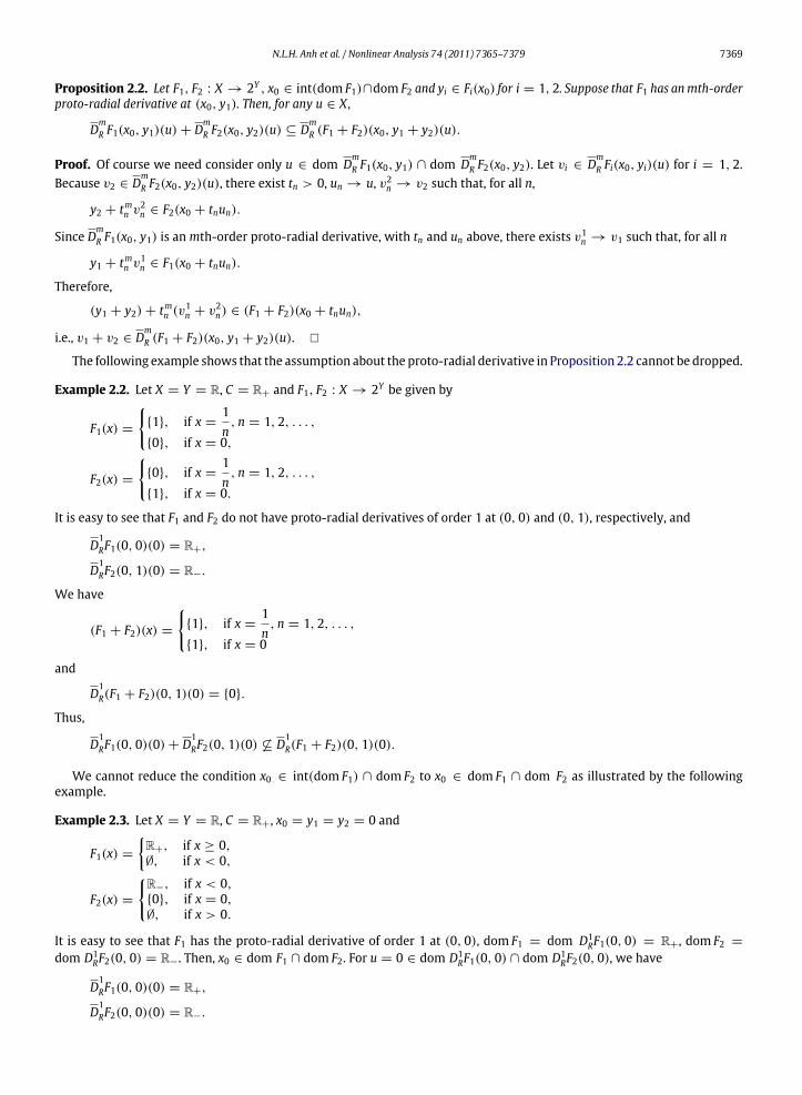
Proposition 2.2. Let F1, F2 : X → 2Y , x0 ∈ int(dom F1)∩dom F2 and yi ∈ Fi(x0) for i = 1, 2. Suppose that F1 has anmth-orderproto-radial derivative at (x0, y1). Then, for any u ∈ X,

DmR F1(x0, y1)(u) + D

mR F2(x0, y2)(u) ⊆ D

mR (F1 + F2)(x0, y1 + y2)(u).

Proof. Of course we need consider only u ∈ dom DmR F1(x0, y1) ∩ dom D

mR F2(x0, y2). Let vi ∈ D

mR Fi(x0, yi)(u) for i = 1, 2.

Because v2 ∈ DmR F2(x0, y2)(u), there exist tn > 0, un → u, v2

n → v2 such that, for all n,

y2 + tmn v2n ∈ F2(x0 + tnun).

Since DmR F1(x0, y1) is anmth-order proto-radial derivative, with tn and un above, there exists v1

n → v1 such that, for all n

y1 + tmn v1n ∈ F1(x0 + tnun).

Therefore,

(y1 + y2) + tmn (v1n + v2

n) ∈ (F1 + F2)(x0 + tnun),

i.e., v1 + v2 ∈ DmR (F1 + F2)(x0, y1 + y2)(u). �

The following example shows that the assumption about the proto-radial derivative in Proposition 2.2 cannot be dropped.

Example 2.2. Let X = Y = R, C = R+ and F1, F2 : X → 2Y be given by

F1(x) =

{1}, if x =

1n, n = 1, 2, . . . ,

{0}, if x = 0,

F2(x) =

{0}, if x =

1n, n = 1, 2, . . . ,

{1}, if x = 0.

It is easy to see that F1 and F2 do not have proto-radial derivatives of order 1 at (0, 0) and (0, 1), respectively, and

D1RF1(0, 0)(0) = R+,

D1RF2(0, 1)(0) = R−.

We have

(F1 + F2)(x) =

{1}, if x =

1n, n = 1, 2, . . . ,

{1}, if x = 0

and

D1R(F1 + F2)(0, 1)(0) = {0}.

Thus,

D1RF1(0, 0)(0) + D

1RF2(0, 1)(0) ⊆ D

1R(F1 + F2)(0, 1)(0).

We cannot reduce the condition x0 ∈ int(dom F1) ∩ dom F2 to x0 ∈ dom F1 ∩ dom F2 as illustrated by the followingexample.

Example 2.3. Let X = Y = R, C = R+, x0 = y1 = y2 = 0 and

F1(x) =

R+, if x ≥ 0,∅, if x < 0,

F2(x) =

R−, if x < 0,{0}, if x = 0,∅, if x > 0.

It is easy to see that F1 has the proto-radial derivative of order 1 at (0, 0), dom F1 = dom D1RF1(0, 0) = R+, dom F2 =

dom D1RF2(0, 0) = R−. Then, x0 ∈ dom F1 ∩ dom F2. For u = 0 ∈ dom D1

RF1(0, 0) ∩ dom D1RF2(0, 0), we have

D1RF1(0, 0)(0) = R+,

D1RF2(0, 0)(0) = R−.

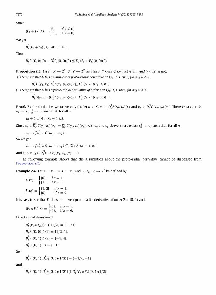
7370 N.L.H. Anh et al. / Nonlinear Analysis 74 (2011) 7365–7379

Since

(F1 + F2)(x) =

∅, if x = 0,R+, if x = 0,

we get

D1R(F1 + F2)(0, 0)(0) = R+.

Thus,

D1RF1(0, 0)(0) + D

1RF2(0, 0)(0) ⊆ D

1R(F1 + F2)(0, 0)(0).

Proposition 2.3. Let F : X → 2Y , G : Y → 2Z with Im F ⊆ dom G, (x0, y0) ∈ gr F and (y0, z0) ∈ grG.

(i) Suppose that G has an mth-order proto-radial derivative at (y0, z0). Then, for any u ∈ X,

DmR G(y0, z0)(D

1RF(x0, y0)(u)) ⊆ D

mR (G ◦ F)(x0, z0)(u).

(ii) Suppose that G has a proto-radial derivative of order 1 at (y0, z0). Then, for any u ∈ X,

D1RG(y0, z0)(D

mR F(x0, y0)(u)) ⊆ D

mR (G ◦ F)(x0, z0)(u).

Proof. By the similarity, we prove only (i). Let u ∈ X , v1 ∈ D1RF(x0, y0)(u) and v2 ∈ D

mR G(y0, z0)(v1). There exist tn > 0,

un → u, v1n → v1 such that, for all n,

y0 + tnv1n ∈ F(x0 + tnun).

Since v2 ∈ DmR G(y0, z0)(v1) = Dm

R G(y0, z0)(v1), with tn and v1n above, there exists v2

n → v2 such that, for all n,

z0 + tmn v2n ∈ G(y0 + tnv1

n).

So we get

z0 + tmn v2n ∈ G(y0 + tnv1

n) ⊆ (G ◦ F)(x0 + tnun)

and hence v2 ∈ DmR (G ◦ F)(x0, z0)(u). �

The following example shows that the assumption about the proto-radial derivative cannot be dispensed fromProposition 2.3.

Example 2.4. Let X = Y = R, C = R+ and F1, F2 : X → 2Y be defined by

F1(x) =

{0}, if x = 1,{1}, if x = 0,

F2(x) =

{1, 2}, if x = 1,{0}, if x = 0.

It is easy to see that F1 does not have a proto-radial derivative of order 2 at (0, 1) and

(F1 ◦ F2)(x) =

{0}, if x = 1,{1}, if x = 0.

Direct calculations yield

D2R(F1 ◦ F2)(0, 1)(1/2) = {−1/4},

D1RF2(0, 0)(1/2) = {1/2, 1},

D2RF1(0, 1)(1/2) = {−1/4},

D2RF1(0, 1)(1) = {−1}.

So

D2RF1(0, 1)[D

1RF2(0, 0)(1/2)] = {−1/4, −1}

and

D2RF1(0, 1)[D

1RF2(0, 0)(1/2)] ⊆ D

2R(F1 ◦ F2)(0, 1)(1/2).

N.L.H. Anh et al. / Nonlinear Analysis 74 (2011) 7365–7379 7371

We now investigate the sumM +N of twomultimapsM,N : X → 2Y . To expressM +N as a composition so that we canapply a chain rule, we define F : X → 2X×Y and G : X × Y → 2Y by, for I being the identity map on X and (x, y) ∈ X × Y ,

F = I × M and G(x, y) = N(x) + y. (1)

Then clearlyM + N = G ◦ F . However, the rule given in Proposition 2.3, though simple and relatively direct, is not suitablefor dealing with these F and G, since the intermediate space (Y there and X × Y here) is little involved. Inspired by [11,22],we develop another composition rule as follows. Let general multimaps F : X → 2Y and G : Y → 2Z be considered now.The so-called resultant multimap R : X × Z → 2Y is defined by

R(x, z) := F(x) ∩ G−1(z).

Then

dom R = gr(G ◦ F).

We define another kind of radial derivative of G ◦ F with a significant role of intermediate variable y as follows.

Definition 2.3. Let (x, z) ∈ gr(G ◦ F) and y ∈ clR(x, z).

(i) Themth-order y-radial derivative of the multimap G ◦ F at (x, z) is the multimap DmR (G ◦y F)(x, z) : X → 2Z given by

DmR (G ◦y F)(x, z)(u) := {w ∈ Z : ∃tn > 0, ∃(un, yn, wn) → (u, y, w),∀n ∈ N, yn ∈ R(x + tnun, z + tmn wn)}.

(ii) Themth-order quasi-derivative of the resultant multimap R at ((x, z), y) is defined by, for (u, w) ∈ X × Z ,

Dmq R((x, z), y)(u, w) := {y ∈ Y : ∃hn → 0+, ∃(un, yn, wn) → (u, y, w),

∀n ∈ N, y + hmn yn ∈ R(x + hnun, z + hm

n wn)}.

One has an obvious relationship between DmR (G ◦y F)(x, z) and D

mR (G ◦ F)(x, z) as noted in the next proposition.

Proposition 2.4. Given (x, z) ∈ gr(G ◦ F), y ∈ clR(x, z) and u ∈ X, one always has

DmR (G ◦y F)(x, z)(u) ⊆ D

mR (G ◦ F)(x, z).

Proof. This follows immediately from the definitions. �

Proposition 2.5. Let (x, z) ∈ gr(G ◦ F), y ∈ clR(x, z) and u ∈ X.

(i) If for all w ∈ Z one has

D1RF(x, y)(u) ∩ D

mR G

−1(z, y)(w) ⊆ Dmq R((x, z), y)(u, w), (2)

then

DmR G(y, z)[D

1RF(x, y)(u)] ⊆ D

mR (G ◦y F)(x, z)(u);

(ii) If (2) holds for all y ∈ clR(x, z), theny∈clR(x,z)

DmR G(y, z)[D

1RF(x, y)(u)] ⊆ D

mR (G ◦ F)(x, z)(u).

Proof. (i) If the left side of the conclusion of (i) is empty we are done. Let v ∈ DmR G(y, z)[D

1RF(x, y)(u)], i.e., there exists

some y ∈ D1RF(x, y)(u) such that y ∈ D

mR G

−1(z, y)(v). Then (2) ensures that y ∈ Dmq R((x, z), y)(u, v). This means the

existence of tn → 0+, (un, yn, vn) → (u, y, v) satisfying

y + tmn yn ∈ R(x + tnun, z + tmn vn).

With yn := y + tmn yn, we have

yn ∈ R(x + tnun, z + tmn vn).

So v ∈ DmR (G ◦y F)(x, z)(u) and we are done.

(ii) Is immediate from (i) and Proposition 2.4. �

7372 N.L.H. Anh et al. / Nonlinear Analysis 74 (2011) 7365–7379

Now we apply the preceding composition rules to establish sum rules for M,N : X → 2Y . For this purpose, we useF : X → 2X×Y and G : X × Y → 2Y defined in (1). Then,M + N = G ◦ F . For (x, z) ∈ X × Y , following [23] we set

S(x, z) := M(x) ∩ (z − N(x)).

Then the resultant multimap R : X × Y → 2X×Y associated to these F and G is

R(x, z) = {x} × S(x, z).

We also modify the definition of y-contingent derivative D(M +y N) in [23] to obtain a kind of radial derivatives as follows.

Definition 2.4. Given (x, z) ∈ dom S and y ∈ clS(x, z), themth-order y-radial derivative ofM +y N at (x, z) is themultimapDmR (M +y N)(x, z) : X → 2Y given by

DmR (M +y N)(x, z)(u) := {w ∈ Y : ∃tn > 0, ∃(un, yn, wn) → (u, y, w),∀n, yn ∈ S(x + tnun, z + tmn wn)}.

Observe that

DmR (M +y N)(x, z)(u) = D

mR (G ◦y F)(x, z)(u).

One has a relationship between DmR (M +y N)(x, z)(u) and D

mR (M + N)(x, z)(u) as follows.

Proposition 2.6. Given (x, z) ∈ gr(M + N) and y ∈ clS(x, z), one always has

DmR (M +y N)(x, z)(u) ⊆ D

mR (M + N)(x, z)(u).

Proof. This is an immediate consequence of the definitions. �

Proposition 2.7. Let (x, z) ∈ gr(M + N) and u ∈ X.

(i) Let y ∈ clS(x, z). If for all v ∈ Y , one has

DmR M(x, y)(u) ∩ [v − D

mR N(x, z − y)(u)] ⊆ D

mq S((x, z), y)(u, v), (3)

then

DmR M(x, y)(u) + D

mR N(x, z − y)(u) ⊆ D

mR (M +y N)(x, z)(u).

(ii) If (3) holds for all y ∈ clS(x, z), theny∈clS(x,z)

DmR M(x, y)(u) + D

mR N(x, z − y)(v) ⊆ D

mR (M + N)(x, z)(u).

Proof. (i) If the left side of the conclusion of (i) is empty, nothing is to be proved. If v ∈ DmR M(x, y)(u) + D

mR N(x, z − y)(u),

there exists some y ∈ DmR M(x, y)(u) such that y ∈ v−D

mR N(x, z−y)(u). Hence, (3) ensures that y ∈ D

mq S((x, z), y)(u, v).

Therefore, there exist tn → 0+, (un, yn, vn) → (u, y, v) such that

y + tmn yn ∈ S(x + tnun, z + tmn vn).

Setting yn := y + tmn yn, we have

yn ∈ S(x + tnun, z + tmn vn).

Consequently, v ∈ DmR (M +y N)(x, z)(u).

(ii) This follows from (i) and Proposition 2.6. �

The following example shows that assumption (3) cannot be dispensed and is not difficult to check.

Example 2.5. Let X = Y = R and M,N : X → 2Y be given by

M(x) =

{1}, if x =

1n, n = 1, 2, . . . ,

{0}, if x = 0,

N(x) =

{0}, if x =

1n, n = 1, 2, . . . ,

{1}, if x = 0.

N.L.H. Anh et al. / Nonlinear Analysis 74 (2011) 7365–7379 7373

Then

S(x, z) = M(x) ∩ (z − N(x)) =

{0}, if (x, z) = (0, 1),

{1}, if (x, z) =

1n, 1

, n = 1, 2, . . . ,

∅, otherwise.

Choose x = 0, z = 1, y = 0 ∈ clS(x, z) and u = v = 0. Then,

D1RM(x, y)(u) = R+,

D1RN(x, z − y)(u) = R−,

D1qS((x, z), y)(u, v) = {0}.

Thus,

D1RM(x, y)(u) ∩ [v − D

1RN(x, z − y)(u)] ⊆ D

1qS((x, z), y)(u, v).

Direct calculations show that the conclusion of Proposition 2.7 does not hold, since

D1R(M +y N)(x, z)(u) = {0}

and hence

D1RM(x, y)(u) + D

1RN(x, z − y)(u) ⊆ D

1R(M +y N)(x, z)(u).

Proposition 2.8. Let F : X → Y , (x0, y0) ∈ gr F , λ > 0 and β ∈ R. Then

(i) DmR (βF)(x0, βy0)(u) = βD

mR F(x0, y0)(u);

(ii) DmR (F)(x0, y0)(λu) = λmD

mR F(x0, y0)(u).

In the remaining part of this section, we apply Propositions 2.2 and 2.3 to establish necessary optimality conditionsfor several types of efficient solutions of some particular optimization problems. (Optimality conditions, using higher-orderradial derivatives, for general optimization problems are discussed in Section 3.) AsQ -minimality includesmany other kindsof solutions as particular cases, we first prove a simple characterization of this notion.

Proposition 2.9. Let X, Y and Q be as before, F : X → 2Y and (x0, y0) ∈ gr F . Then y0 is a Q -minimal point of F(X) if andonly if

DmR F(x0, y0)(X) ∩ (−Q ) = ∅. (4)

Proof. ‘‘Only if’’ suppose to the contrary that y0 is aQ -minimal point of F(X) but there exist x ∈ X and y ∈ DmR (F , x0, y0)(x)∩

(−Q ). There exist sequences tn > 0, xn → x and yn → y such that, for all n,

y0 + tmn yn ∈ F(x0 + tnxn).

Since the cone Q is open, we have tmn yn ∈ −Q for n large enough. Therefore,

tmn yn ∈ (F(x0 + tnxn) − y0) ∩ (−Q ),

a contradiction.‘‘If’’ assume that (4) holds. From Proposition 2.1 one has, for all x ∈ X ,

(F(x) − y0) ∩ (−Q ) ⊆ DmR F(x0, y0)(x − x0) ∩ (−Q ) = ∅.

This means that y0 is a Q -minimal point of F(X). �

Let X and Y be normed spaces, Y being partially ordered by a pointed closed convex cone C with nonempty interior,F : X → 2Y and G : X → 2X . Consider the problem

(P1) min F(x′) subject to x ∈ X and x′∈ G(x).

This problem can be restated as the following unconstrained problem: min(F ◦ G)(x). Recall that (x0, y0) is said to be aQ -minimal solution of (P2) if y0 ∈ (F ◦ G)(x0) and ((F ◦ G)(X) − y0) ∩ (−Q ) = ∅.

Proposition 2.10. Let ImG ⊆ dom F , (x0, z0) ∈ grG and (z0, y0) ∈ gr F . Assume that (x0, y0) is a Q -minimal solution of (P1).(i) If F has an mth-order proto-radial derivative at (z0, y0) then, for any u ∈ X,

DmR F(z0, y0)(D

1RG(x0, z0)(u)) ∩ (−Q ) = ∅. (5)

7374 N.L.H. Anh et al. / Nonlinear Analysis 74 (2011) 7365–7379

(ii) If F has a proto-radial derivative of order1 at (z0, y0) then, for any u ∈ X,

D1RF(z0, y0)(D

mR G(x0, z0)(u)) ∩ (−Q ) = ∅. (6)

Proof. By the similarity, we prove only (i). From Proposition 2.9, we have

DmR ((F ◦ G))(x0, y0) ∩ (−Q ) = ∅.

Proposition 2.3(i) says that

DmR F(z0, y0)(D

1RG(x0, z0)(u)) ⊆ D

mR (F ◦ G)(x0, y0)(u).

So

DmR F(z0, y0)(D

1RG(x0, z0)(u)) ∩ (−Q ) = ∅. �

Later on we adopt the usual convention that for x0 being feasible, (x0, y0) is a solution in a sense of a vector optimizationproblem if and only if y0 is the efficient point in this sense of the image of the feasible set, in the objective space. Then, fromPropositions 2.1 and 2.10 we obtain the following theorem.

Theorem 2.11. Let the assumptions of Proposition 2.10 be satisfied and (x0, y0) ∈ grF . Then (5) and (6) hold in each of thefollowing cases

(i) (x0, y0) is a strong efficient solution of (P1) and Q = Y \ (−C);(ii) (x0, y0) is a weak efficient solution of (P1) and Q = int C;(iii) (x0, y0) is a positive-properly efficient solution of (P1) and Q = {y : ϕ(y) > 0} for some functional ϕ ∈ C+i;(iv) (x0, y0) is a Geoffrion-properly efficient solution of (P1) and Q = C(ϵ) for some ϵ > 0 (C(ϵ) = {y ∈ Y : dC (y) <

ϵd−C (y)});(v) (x0, y0) is a Borwein-properly efficient solution of (P1) and Q = K for some open cone K dilating C;(vi) (x0, y0) is a Henig-properly efficient solution of (P1) and Q = K for some open convex cone K dilating C;(vii) (x0, y0) is a strong Henig-properly efficient solution of (P1) and Q = int Cϵ(B) for some ϵ satisfying 0 < ϵ < δ (B is a base

of C, Cϵ(B) = cone(B + ϵBY ) and δ = inf{‖b‖ : b ∈ B});(viii) (x0, y0) is a super efficient solution of (P1) and Q = int Cϵ(B) for ϵ satisfying 0 < ϵ < δ.

To compare with a result in [22], we recall the definition of contingent epiderivatives. For amultimap F between normedspaces X and Y , Y being partially ordered by a pointed convex cone C and a point (x, y) ∈ gr F , a single-valued mapEDF(x, y) : X → Y satisfying epi(EDF(x, y)) = TepiF (x, y) ≡ Tgr F+(x, y) is said to be the contingent epiderivative of Fat (x, y).

Example 2.6. Let X = Y = R, C = R+, G(x) = {−|x|} and F be defined by

F(x) =

R−, if x ≤ 0,∅, if x > 0.

Since G is single-valued, we try to make use of Proposition 5.2 of [22]. By a direct computation, we have DG(0,G(0))(h) =

{−|h|} for all h ∈ X and TepiF (G(0), 0) = R2 and hence the contingent epiderivative EDF(G(0), 0)(h) does not exist for anyh ∈ X . Therefore, the necessary condition in the mentioned proposition of [22] cannot be applied. However, F has an mth-order proto-radial derivative at (G(0), 0) and D

1R(0,G(0))(0) = {0}, D

mR F(G(0), 0)[D

1RG(0,G(0))(0)] = R−, which meets

−int C and hence Proposition 2.10 above rejects the candidate for a weak solution.

To illustrate sum rules, we consider the following problem

(P2) min F(x) subject to g(x) ≤ 0,

where X , Y are as for problem (P2), F : X → 2Y and g : X → Y . Denote S = {x ∈ X | g(x) ≤ 0} (the feasible set). DefineG : X → 2Y by

G(x) =

{0}, if x ∈ S,{g(x)}, otherwise.

Consider the following unconstrained set-valued optimization problem, for an arbitrary positive s,

(PC) min(F + sG)(x).

In the particular case, where Y = R and F is single-valued, (PC) is used to approximate (P2) in penaltymethods (see [24]).Optimality conditions for this general problem (PC) are obtained in [11] using calculus rules for variational sets and in [22] byusing such rules for contingent epiderivatives. Here we will apply Propositions 2.2 and 2.8 for mth-order radial derivativesto get the following necessary condition for several types of efficient solutions of (PC).

N.L.H. Anh et al. / Nonlinear Analysis 74 (2011) 7365–7379 7375

Proposition 2.12. Let dom F ⊆ dom G, x0 ∈ S, y0 ∈ F(x0) and either F or G has an mth-order proto-radial derivative at(x0, y0) or (x0, 0), respectively. If (x0, y0) is a Q -minimal solution of (PC) then, for any u ∈ X,

(DmR F(x0, y0)(u) + sD

mR G(x0, 0)(u)) ∩ −Q = ∅. (7)

Proof. Weneed to discuss only u ∈ domDmR F(x0, y0)∩domD

mR G(x0, 0). By Proposition 2.9, one getsD

mR (F +sG)(x0, y0)(u)∩

−Q = ∅. According to Proposition 2.8, sDmR G(x0, 0)(u) = D

mR (sG)(x0, 0)(u). Then, Proposition 2.2 yields

DmR F(x0, y0)(u) + sD

mR G(x0, 0)(u) ⊆ D

mR (F + sG)(x0, y0 + 0)(u).

The proof is complete. �

Similarly as stated in Theorem 2.11, formula (8) holds true for each of our eight kinds of efficient solutions of (P2), withQ being chosen correspondingly. The next example illustrates a case, Proposition 2.12 is more advantageous than earlierexisting results.

Example 2.7. Let X = Y = R, C = R+, g(x) = x4 − 2x3 and

F(x) =

R−, if x ≤ 0,∅, if x > 0.

Then S = [0, 2] and G(x) = {max{0, x4 − 2x3}}. Furthermore, since TepiF (0, 0) = R2, TepiG(0, 0) = {(x, y), y ≥ 0},the contingent epiderivative DF(0, 0)(h) does not exist for any h ∈ X and Proposition 5.1 of [22] cannot be employed.But F has a proto-radial derivative of order 1 at (0, 0), D

1RF(0, 0)(0) = R− and {0} ⊆ D

1RG(0, 0)(0) ⊆ R+. So,

D1RF(0, 0)(0) + sD

1RG(0, 0)(0) ∩ (−int C) = ∅. By Proposition 2.12, (x0, y0) is not a weak efficient solution of (PC). This

fact can be checked directly too.

3. Optimality conditions

Let X and Y be normed spaces partially ordered by pointed closed convex cones C and D, respectively, with nonemptyinterior. Let S ⊆ X, F : X → 2Y and G : X → 2Z . In this section, we discuss optimality conditions for the following generalset-valued vector optimization problem with inequality constraints

(P) min F(x), subject to x ∈ S, G(x) ∩ (−D) = ∅.

Let A := {x ∈ S : G(x) ∩ (−D) = ∅} and F(A) :=

x∈A F(x). We assume that F(x) = ∅ for all x ∈ X .

Proposition 3.1. Let dom F ∪ dom G ⊆ S and (x0, y0) is a Q -minimal solution for (P). Then, for any z0 ∈ G(x0) ∩ (−D) andx ∈ X,

DmR (F ,G)(x0, y0)(x) ∩ (−Q × −intD) = ∅. (8)

Proof. We need to investigate only x ∈ dom DmR (F ,G)(x0, y0). For all x ∈ A,

(F(x) − y0) ∩ (−Q ) = ∅.

Suppose (8) does not hold. Then, there exists x ∈ dom DmR (F ,G)(x0, y0) such that

(y, z) ∈ DmR (F ,G)(x0, y0)(x) (9)

and

(y, z) ∈ −Q × −intD. (10)

It follows from (9) that there exist {tn} with tn > 0 and {(xn, yn, zn)} in X × Y × Z with (xn, yn, zn) → (x, y, z) such that

(y0, z0) + tmn (yn, zn) ∈ (F ,G)(x0 + tnxn).

Hence, xn := x0 + tnxn ∈ dom (F ,G) ⊆ S and there exists (yn, zn) ∈ (F ,G)(xn) such that

(y0, z0) + tmn (yn, zn) = (yn, zn).

As (yn, zn) → (y, z), this implies that

yn − y0tmn

→ y, (11)

7376 N.L.H. Anh et al. / Nonlinear Analysis 74 (2011) 7365–7379

and

zn − z0tmn

→ z. (12)

Combining (10)–(12), one finds N > 0 such that, for n ≥ N ,

yn − y0tmn

∈ −Q , (13)

andzn − z0

tmn∈ −intD.

Thus, zn ∈ −D. Hence, xn ∈ A for large n.On the other hand, by (13) we get, for n ≥ N ,

yn − y0 ∈ −Q .

This is a contradiction. So, (8) holds. �

From Propositions 3.1 and 1.2, we obtain immediately the following result.

Theorem 3.2. Assume that dom F ∪ dom G ⊆ S. Then (8) holds in each of the following cases

(i) (x0, y0) is a strong efficient solution of (P) and Q = Y \ −C;(ii) (x0, y0) is a weak efficient solution of (P) and Q = int C;(iii) (x0, y0) is a positive-properly efficient solution of (P) and Q = {y : ϕ(y) > 0} for some functional ϕ ∈ C+i;(iv) (x0, y0) is a Geoffrion-properly efficient solution of (P) and Q = C(ϵ) for some scalar ϵ > 0;(v) (x0, y0) is a Borwein-properly efficient solution of (P) and Q = K for some open cone K dilating C;(vi) (x0, y0) is a Henig-properly efficient solution of (P) and Q = K for some open convex cone K dilating C;(vii) (x0, y0) is a strong Henig-properly efficient solution of (P) and Q = int Cϵ(B) for some ϵ satisfying 0 < ϵ < δ;(viii) (x0, y0) is a super efficient solution of (P) and Q = int Cϵ(B) for some ϵ satisfying 0 < ϵ < δ.

For the comparison purpose, we recall from [12] that the (first-order) variational set of type 2 of F : X → 2Y at (x0, y0) is

W 1(F , x0, y0) = lim supx

F−→x0

cone+(F(x) − y0),

where xF

−→ x0 means that x → x0 and x ∈ dom F . A multimap H : X → 2Y is called pseudoconvex at (x0, y0) ∈ grH if

epi H ⊆ (x0, y0) + Tepi H(x0, y0).

The following example shows a case where many existing theorems using other generalized derivatives do not work,while Theorem 3.2 rejects a candidate for a weak efficient solution.

Example 3.1. Let X = Y = R, C = R+ and F be defined by

F(x) =

[1, +∞), if x = 0,R+, if x = 1,∅, otherwise.

Let (x0, y0) = (0, 1) and u = 1. Then

W 1(F+, x0, y0) = R+.

Hence, Theorem 3.2 of [12] says nothing about (x0, y0). From Remark 2.2(i) and Proposition 4.1 of [12], we see that Theorem7 of [8], Theorem 5 of [25], Theorem 4.1 of [26], Proposition 3.1–3.2, and Theorem 4.1 of [5] cannot be applied to reject(x0, y0) as a candidate for a weak efficient solution.

On the other hand,

D1RF(x0, y0)(u) = [−1, +∞).

Then, D1RF(x0, y0)(u) ∩ (−int C) = ∅. It follows from Theorem 3.2(ii) that (x0, y0) is not a weak efficient solution.

The following example explains that we have to use higher-order radial derivatives instead of lower-order ones whenapplying Theorem 3.2 in some cases.

N.L.H. Anh et al. / Nonlinear Analysis 74 (2011) 7365–7379 7377

Example 3.2. Let X = Y = R, C = R+ and F be defined by

F(x) =

{0}, if x = 0,

{|x|}, if x = −1n, n = 1, 2, . . . ,

{−1}, if x =1n, n = 1, 2, . . . ,

∅, otherwise.

Let (x0, y0) = (0, 0) and u = 0. Then

D1RF(x0, y0)(u) = {0},

D2RF(x0, y0)(u) = R.

Because D2RF(x0, y0)(u) ∩ (−int C) = ∅, (x0, y0) is not a weak efficient solution. (But D

1RF(x0, y0) cannot be used here.)

We have seen that our necessary optimality conditions using radial derivatives are stronger than many existingconditions using other generalized derivatives, since images of a point or set through radial derivatives are larger than thecorresponding images through other derivatives. The next proposition gives a sufficient condition, which has a reasonablegap with the corresponding necessary condition in Proposition 3.1.

Proposition 3.3. Let dom F ∪ dom G ⊆ S, x0 ∈ A, y0 ∈ F(x0) and z0 ∈ G(x0) ∩ (−D). Then (x0, y0) is a Q -minimal solutionof (P) if the following condition holds

DmR (F ,G)(x0, y0)(A − x0) ∩ −(Q × D(z0)) = ∅. (14)

Proof. From Proposition 2.1, for x ∈ A one has

(F ,G)(x) − (y0, z0) ⊆ DmR (F ,G)(x0, y0)(x − x0).

Then

(F ,G)(x) − (y0, z0) ∩ −(Q × D(z0)) = ∅. (15)

Suppose the existence of x ∈ A and y ∈ F(x) such that y − y0 ∈ −Q . For any z ∈ G(x) ∩ (−D) one has z − z0 ∈ −D(z0) andhence (y, z) − (y0, z0) ∈ −(Q × D(z0)), contradicting (15). �

A natural question now arises: can we replace D by D(z0) in the necessary condition given by Proposition 3.1 to obtaina smaller gap with the sufficient one expressed by Proposition 3.3? Unfortunately, a negative answer is supplied by thefollowing example.

Example 3.3. Suppose that X = Y = Z = R, S = X , C = D = R+ and F : X → 2Y and G : X → 2Z are given by

F(x) =

{y : y ≥ x2}, if x ∈ [−1, 1],{−1}, if x ∈ [−1, 1],

G(x) = {z ∈ Z : z = x2 − 1}.

We have A = [−1, 1] in problem (P). It easy to see that (x0, y0) = (0, 0) is a weak efficient solution of (P). So the conditionof Theorem 3.2(ii) is satisfied. Take z0 = −1 ∈ G(x0) ∩ (−D). Since for all x ∈ X , D

2R(F ,G)(x0, y0, z0)(x) ⊆ R × R+, we have

D2R(F ,G)(x0, y0, z0)(x) ∩ −int(C × D) = ∅.

On the other hand, D(z0) = R. We claim the existence of x ∈ X such that

D2R(F ,G)(x0, y0, z0)(x) ∩ −int(C × D(z0)) = ∅.

Indeed, choose x > 0, xn = x and tn =2xn. Then

(y0, z0) + t2n (vn, wn) ∈ (F ,G)(x0 + tnxn)

means that

(0, −1) +4x2

(vn, wn) ∈ (F ,G)(2),

7378 N.L.H. Anh et al. / Nonlinear Analysis 74 (2011) 7365–7379

i.e.,

4x2

vn = −1,4x2

wn = 4.

So, there exist vn =−x24 →

−x24 ∈ −int C and wn = x2 → x2 ∈ −intD(z0). Thus,

−x24 , x2

∈ D

2R(F ,G)(x0, y0, z0)(x).

Similarly as before, from an assertion for Q -minimal solutions we always obtain the corresponding ones for our eightkinds of efficient solutions. Hence we arrive at the following sufficient conditions.

Theorem 3.4. Assume that dom F ∪ dom G ⊆ S, x0 ∈ A, y0 ∈ F(x0) and z0 ∈ G(x0) ∩ (−D). Let condition (14) hold. Then

(i) (x0, y0) is a strong efficient solution of (P) if Q = Y \ −C;(ii) (x0, y0) is a weak efficient solution of (P) if Q = int C;(iii) (x0, y0) is a positive-properly efficient solution of (P) if Q = {y : ϕ(y) > 0} for some functional ϕ ∈ C+i;(iv) (x0, y0) is a Geoffrion-properly efficient solution of (P) if Q = C(ϵ) for some scalar ϵ > 0;(v) (x0, y0) is a Borwein-properly efficient solution of (P) if Q = K for some open cone K dilating C;(vi) (x0, y0) is a Henig-properly efficient solution of (P) if Q = K for some open convex cone K dilating C;(vii) (x0, y0) is a strong Henig-properly efficient solution of (P) if Q = int Cϵ(B) for some scalar ϵ satisfying 0 < ϵ < δ;(viii) (x0, y0) is a super efficient solution of (P) if Q = int Cϵ(B) for some scalar ϵ satisfying 0 < ϵ < δ.

We illustrate advantages of Theorem 3.4 by showing a case where it works while many earlier results do not in thefollowing example.

Example 3.4. Let X = Y = R, C = R+ and F be defined by

F(x) =

{0}, if x = 0,

1n2

, if x = n for n = 1, 2, . . . ,

∅, otherwise.

Let (x0, y0) = (0, 0) and u ∈ dom D1RF(x0, y0) = R+. Then, for n = 1, 2 . . .,

D1RF(x0, y0)(u) =

un3

{0}.

It follows from Theorem 3.4(ii) that (x0, y0) is a weak efficient solution. It is easy to see that dom F = {0, 1, 2, . . .} is notconvex and F is not pseudoconvex at (x0, y0). So Theorem 8 of [8], Theorem 6 of [25] and Theorem 3.3 of [12] cannot beused.

Acknowledgments

This work was supported by National Foundation for Science and Technology Development of Viet Nam. The authors aregrateful to a referee for valuable remarks helping them to improve the paper.

References

[1] B.S. Mordukhovich, Variational Analysis and Generalized Differentiation, Vol. I–Basic Theory, Springer, Berlin, 2006.[2] B.S. Mordukhovich, Variational Analysis and Generalized Differentiation, Vol. II–Applications, Springer, Berlin, 2006.[3] J.P. Aubin, Contingent derivatives of set-valuedmaps and existence of solutions in nonlinear inclusions and differential inclusions, in: L. Nachbin (Ed.),

Advances in Mathematics, Supplementary Studies 7A, Academic Press, New York, 1981, pp. 160–232.[4] J.-P. Aubin, H. Frankowska, Set-Valued Analysis, Birkhauser, Boston, 1990.[5] A. Taa, Set-valued derivatives of multifunctions and optimality conditions, Numer. Funct. Anal. Optim. 19 (1998) 121–140.[6] F. Flores-Bazan, Optimality conditions in non-convex set-valued optimization, Math. Methods Oper. Res. 53 (2001) 403–417.[7] F. Flores-Bazan, Radial epiderivatives and asymptotic function in nonconvex vector optimization, SIAM J. Optim. 14 (2003) 284–305.[8] J. Jahn, R. Rauh, Contingent epiderivatives and set-valued optimization, Math. Methods Oper. Res. 46 (1997) 193–211.[9] R. Kasimbeyli, Radial epiderivatives and set-valued optimization, Optimization 58 (2009) 521–534.

[10] F. Flores-Bazan, B. Jimenez, Strict efficiency in set-valued optimization, SIAM J. Control Optim. 48 (2009) 881–908.[11] N.L.H. Anh, P.Q. Khanh, L.T. Tung, Variational sets: calculus and applications to nonsmooth vector optimization, Nonlinear Anal. TMA 74 (2011)

2358–2379.[12] P.Q. Khanh, N.D. Tuan, Variational sets of multivaluedmappings and a unified study of optimality conditions, J. Optim. Theory Appl. 139 (2008) 45–67.[13] P.Q. Khanh, N.D. Tuan, Higher-order variational sets and higher-order optimality conditions for proper efficiency in set-valued nonsmooth vector

optimization, J. Optim. Theory Appl. 139 (2008) 243–261.[14] M. Studniarski, Higher-order necessary optimality conditions in terms of Neustadt derivatives, Nonlinear Anal. 47 (2001) 363–373.[15] B. Jimenez, V. Novo, Higher-order optimality conditions for strict local minima, Ann. Oper. Res. 157 (2008) 183–192.[16] T.D.X. Ha, Optimality conditions for several types of efficient solutions of set-valued optimization problems, in: P. Pardalos, Th.M. Rassis, A.A. Khan

(Eds.), Nonlinear Analysis and Variational Problems, Springer, 2009, pp. 305–324 (Chapter 21).[17] P.Q. Khanh, Proper solutions of vector optimization problems, J. Optim. Theory Appl. 74 (1992) 105–130.[18] A. Guerraggio, E. Molho, A. Zaffaroni, On the notion of proper efficiency in vector optimization, J. Optim. Theory Appl. 82 (1994) 1–21.[19] E.K. Makarov, N.N. Rachkovski, Unified representation of proper efficiency by means of dilating cones, J. Optim. Theory Appl. 101 (1999) 141–165.

N.L.H. Anh et al. / Nonlinear Analysis 74 (2011) 7365–7379 7379

[20] P.Q. Khanh, Optimality conditions via norm scalarization in vector optimization, SIAM J. Control Optim. 31 (1993) 646–658.[21] N.L.H. Anh, P.Q. Khanh, Optimality conditions in set-valued optimization using radial sets and radial derivatives (submitted for publication).[22] J. Jahn, A.A. Khan, Some calculus rules for contingent epiderivatives, Optimization 52 (2003) 113–125.[23] S.J. Li, K.W. Meng, J.-P. Penot, Calculus rules for derivatives of multimaps, Set-Valued Anal. 17 (2009) 21–39.[24] R.T. Rockafellar, R.J.-B Wets, Variational Analysis, third ed., Springer, Berlin, 2009.[25] Y. Chen, J. Jahn, Optimality conditions for set-valued optimization problems, Math. Methods Oper. Res. 48 (1998) 187–200.[26] W. Corley, Optimality conditions for maximization of set-valued functions, J. Optim. Theory Appl. 58 (1988) 1–10.