DISCRETE MATHEMATICS
124
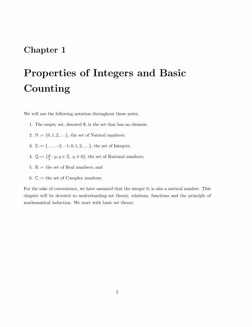
Chapter 1 Properties of Integers and Basic Counting We will use the following notation throughout these notes. 1. The empty set, denoted ∅, is the set that has no element. 2. N := {0, 1, 2,... }, the set of Natural numbers; 3. Z := {..., −2, −1, 0, 1, 2,... }, the set of Integers; 4. Q := { p q : p,q ∈ Z,q =0}, the set of Rational numbers; 5. R := the set of Real numbers; and 6. C := the set of Complex numbers. For the sake of convenience, we have assumed that the integer 0, is also a natural number. This chapter will be devoted to understanding set theory, relations, functions and the principle of mathematical induction. We start with basic set theory. 5
Transcript of DISCRETE MATHEMATICS
Chapter 1
Properties of Integers and Basic
Counting
We will use the following notation throughout these notes.
1. The empty set, denoted ∅, is the set that has no element.
2. N := 0, 1, 2, . . ., the set of Natural numbers;
3. Z := . . . ,−2,−1, 0, 1, 2, . . ., the set of Integers;
4. Q := pq : p, q ∈ Z, q 6= 0, the set of Rational numbers;
5. R := the set of Real numbers; and
6. C := the set of Complex numbers.
For the sake of convenience, we have assumed that the integer 0, is also a natural number. This
chapter will be devoted to understanding set theory, relations, functions and the principle of
mathematical induction. We start with basic set theory.
5
6 CHAPTER 1. PROPERTIES OF INTEGERS AND BASIC COUNTING
1.1 Basic Set Theory
We have already seen examples of sets, such as N,Z,Q,R and C at the beginning of this chapter.
For example, one can also look at the following sets.
Example 1.1.1. 1. 1, 3, 5, 7, . . ., the set of odd natural numbers.
2. 0, 2, 4, 6, . . ., the set of even natural numbers.
3. . . . ,−5,−3,−1, 1, 3, 5, . . ., the set of odd integers.
4. . . . ,−6,−4,−2, 0, 2, 4, 6, . . ., the set of even integers.
5. 0, 1, 2, . . . , 10.
6. 1, 2, . . . , 10.
7. Q+ = x ∈ Q : x > 0, the set of positive rational numbers.
8. R+ = x ∈ R : x > 0, the set of positive real numbers.
9. Q∗ = x ∈ Q : x 6= 0, the set of non-zero rational numbers.
10. R∗ = x ∈ R : x 6= 0, the set of non-zero real numbers.
We observe that the sets that appear in Example 1.1.1 have been obtained by picking certain
elements from the sets N,Z,Q,R or C. These sets are example of what are called “subsets of a
set”, which we define next. We also define certain operations on sets.
Definition 1.1.2 (Subset, Complement, Union, Intersection). 1. Let A be a set. If B is a
set such that each element of B is also an element of the set A, then B is said to be a
subset of the set A, denoted B ⊆ A.
2. Two sets A and B are said to be equal if A ⊆ B and B ⊆ A, denoted A = B.
3. Let A be a subset of a set Ω. Then the complement of A in Ω, denoted A′, is a set that
contains every element of Ω that is not an element of A. Specifically, A′ = x ∈ Ω : x 6∈ A.
4. Let A and B be two subsets of a set Ω. Then their
(a) union, denoted A ∪ B, is the set that exactly contains all the elements of A and all
the elements of B. To be more precise, A ∪B = x ∈ Ω : x ∈ A or x ∈ B.
(b) intersection, denoted A ∩B, is the set that exactly contains those elements of A that
are also elements of B. To be more precise, A ∩B = x ∈ Ω : x ∈ A and x ∈ B.
Example 1.1.3. 1. Let A be a set. Then A ⊆ A.
1.1. BASIC SET THEORY 7
2. The empty set is a subset of every set.
3. Observe that N ⊆ Z ⊆ Q ⊆ R ⊆ C.
4. As mentioned earlier, all examples that appear in Example 1.1.1 are subsets of one or more
sets from N,Z,Q,R and C.
5. Let A be the set of odd integers and B be the set of even integers. Then A ∩ B = ∅ and
A∪B = Z. Thus, it also follows that the complement of A, in Z, equals B and vice-versa.
6. Let A = b, c, b, c and B = a, b, c be subsets of a set Ω. Then A ∩ B = ∅ and
A ∪B = a, b, c, b, c, b, c .
Definition 1.1.4 (Cardinality). A set A is said to have finite cardinality, denoted |A|, if thenumber of distinct elements in A is finite, else the set A is said to have infinite cardinality.
Example 1.1.5. 1. The cardinality of the empty set equals 0. That is, |∅| = 0.
2. Fix a positive integer n and consider the set A = 1, 2, . . . , n. Then |A| = n.
3. Let S = 2x ∈ Z : x ∈ Z. Then S is the set of even integers and it’s cardinality is infinite.
4. Let A = a1, a2, . . . , am and B = b1, b2, . . . , bn be two finite subsets of a set Ω, with
|A| = m and B| = n. Also, assume that A ∩B = ∅. Then, by definition it follows that
A ∪B = a1, a2, . . . , am, b1, b2, . . . , bn
and hence |A ∪B| = |A|+ |B|.
5. Let A = a1, a2, . . . , am and B = b1, b2, . . . , bn be two finite subsets of a set Ω. Then
|A ∪ B| = |A| + |B| − |A ∩ B|. Observe that Example 1.1.5.4 is a particular case of this
result, when A ∩B = ∅.
6. Let A = a1, a2, . . . , am be a collection of singletons of a set Ω. Now choose
an element a ∈ Ω such that a 6= ai, for any i, 1 ≤ i ≤ n. Then verify that the set
B = S ∪a : S ∈ A equals a, a1, a, a2, . . . , a, am. Also, observe that A∩B = ∅and |B| = |A|.
Definition 1.1.6 (Power Set). Let A be a subset of a set Ω. Then the set that contains all
subsets of A is called the power set of A and is denoted by P(A) or 2A.
Example 1.1.7. 1. Let A = ∅. Then P(∅) = ∅, A = ∅.
2. Let A = ∅. Then P(A) = ∅, A = ∅, ∅.
3. Let A = a, b, c. Then P(A) = ∅, a, b, c, a, b, a, c, b, c, a, b, c.
4. Let A = b, c, b, c. Then P(A) = ∅, b, c, b, c, b, c, b, c .

8 CHAPTER 1. PROPERTIES OF INTEGERS AND BASIC COUNTING
1.2 Well Ordering Principle and the Principle of Mathematical
Induction
Axiom 1.2.1 (Well-Ordering Principle). Every non-empty subset of natural numbers contains
its least element.
We will use Axiom 1.2.1 to prove the weak form of the principle of mathematical induction.
The proof is based on contradiction. That is, suppose that we need to prove that “whenever the
statement P holds true, the statement Q holds true as well”. A proof by contradiction starts
with the assumption that “the statement P holds true and the statement Q does not hold true”
and tries to arrive at a contradiction to the validity of the statement P being true.
Theorem 1.2.2 (Principle of Mathematical Induction: Weak Form). Let P (n) be a statement
about a positive integer n such that
1. P (1) is true, and
2. P (k + 1) is true whenever one assumes that P (k) is true.
Then P (n) is true for all positive integer n.
Proof. On the contrary, assume that there exists n0 ∈ N such that P (n0) is not true. Now,
consider the set
S = m ∈ N : P (m) is false .
As n0 ∈ S, S 6= ∅. So, by Well-Ordering Principle, S must have a least element, say N . By
assumption, N 6= 1 as P (1) is true. Thus, N ≥ 2 and hence N − 1 ∈ N.Therefore, from the assumption that N is the least element in S and S contains all those
m ∈ N for which P (m) is false, one deduces that P (N − 1) holds true as N − 1 < N ≤ 2. Thus,
the implication “P (N − 1) is true” and Hypothesis 2 imply that P (N) is true.
This leads to a contradiction and hence our first assumption that there exists n0 ∈ N, suchthat P (n0) is not true is false.
Example 1.2.3. 1. Prove that 1 + 2 + · · · + n =n(n+ 1)
2.
Solution: Verify that the result is true for n = 1. Hence, let the result be true for n. Let
us now prove it for n + 1. That is, one needs to show that 1 + 2 + · · · + n + (n + 1) =(n+ 1)(n + 2)
2.
Using Hypothesis 2,
1 + 2 + · · ·+ n+ (n+ 1) =n(n+ 1)
2+ (n+ 1) =
n+ 1
2(n+ 2) .
Thus, by the principle of mathematical induction, the result follows.

1.2. WELL ORDERING PRINCIPLE AND THE PRINCIPLEOFMATHEMATICAL INDUCTION9
2. Prove that 12 + 22 + · · ·+ n2 =n(n+ 1)(2n + 1)
6.
Solution: The result is clearly true for n = 1. Hence, let the result be true for n and one
needs to show that 12 + 22 + · · ·+ n2 + (n+ 1)2 =(n+ 1)(n + 2) (2(n+ 1) + 1)
6.
Using Hypothesis 2,
12 + 22 + · · ·+ n2 + (n+ 1)2 =n(n+ 1)(2n + 1)
6+ (n+ 1)2
=n+ 1
6(n(2n+ 1) + 6(n+ 1))
=n+ 1
6
(2n2 + 7n+ 6
)=
(n+ 1)(n + 2) (2n+ 3)
6.
Thus, by the principle of mathematical induction, the result follows.
3. Prove that for any positive integer n, 1 + 3 + · · ·+ (2n − 1) = n2.
Solution: The result is clearly true for n = 1. Let the result be true for n. That is,
1 + 3 + · · · + (2n− 1) = n2. Now, we see that
1 + 3 + · · ·+ (2n − 1) + (2n+ 1) = n2 + (2n + 1) = (n+ 1)2.
Thus, by the principle of mathematical induction, the result follows.
4. AM-GM Inequality: Let n ∈ N and suppose we are given real numbers a1 ≥ a2 ≥ · · · ≥an ≥ 0. Then
Arithmetic Mean (AM) :=a1 + a2 + · · ·+ an
n≥ n
√a1 · a2 · · · · · an =: (GM) Geometric Mean.
Solution: The result is clearly true for n = 1, 2. So, we assume the result holds for any
collection of n non-negative real numbers. Need to prove AM ≥ GM, for any collection of
non-negative integers a1 ≥ a2 ≥ · · · ≥ an ≥ an+1 ≥ 0.
So, let us assume that A =a1 + a2 + · · · + an + an+1
n+ 1. Then, it can be easily verified that
a1 ≥ A ≥ an+1 and hence a1 − A, A − an+1 ≥ 0. Thus, (a1 − A)(A − an+1) ≥ 0. Or
equivalently,
A(a1 + an+1 −A) ≥ a1an+1. (1.1)
Now, according to our assumption, the AM-GM inequality holds for any collection of n
non-negative numbers. Hence, in particular, for the collection a2, a3, . . . , an, a1+an+1−A.That is,
AM =a2 + · · ·+ an + (a1 + an+1 −A)
n≥ n√
a2 · · · an · (a1 + an+1 −A) = GM. (1.2)
Buta2 + a3 + · · ·+ an + (a1 + an+1 −A)
n= A. Thus, by Equation (1.1) and Equation (1.2),
one has
An+1 ≥ (a2 · a3 · · · · · an · (a1 + an+1 −A)) ·A ≥ (a2 · a3 · · · · · an) a1an+1.
10 CHAPTER 1. PROPERTIES OF INTEGERS AND BASIC COUNTING
Therefore, we see that by the principle of mathematical induction, the result follows.
5. Fix a positive integer n and let A be a set with |A| = n. Then prove that P(A) = 2n.
Solution: Using Example 1.1.7, it follows that the result is true for n = 1. Let the result
be true for all subset A, for which |A| = n. We need to prove the result for a set A that
contains n+ 1 distinct elements, say a1, a2, . . . , an+1.
Let B = a1, a2, . . . , an. Then B ⊆ A, |B| = n and by induction hypothesis, |P(B)| = 2n.
Also, P(B) = S ⊆ a1, a2, . . . , an, an+1 : an+1 6∈ S. Therefore, it can be easily verified
that
P(A) = P(B) ∪ S ∪ an+1 : S ∈ P(B).
Also, note that P(B) ∩ S ∪ an+1 : S ∈ P(B) = ∅, as an+1 6∈ S, for all S ∈ P(B).
Hence, using Examples 1.1.5.4 and 1.1.5.6, we see that
|P(A)| = |P(B)| + |S ∪ an+1 : S ∈ P(B)| = |P(B)| + |P(B)| = 2n + 2n = 2n+1.
Thus, the result holds for any set that consists of n+1 distinct elements and hence by the
principle of mathematical induction, the result holds for every positive integer n.
We state a corollary of the Theorem 1.2.2 without proof. The readers are advised to prove
it for the sake of clarity.
Corollary 1.2.4 (Principle of Mathematical Induction). Let P (n) be a statement about a pos-
itive integer n such that for some fixed positive integer n0,
1. P (n0) is true,
2. P (k + 1) is true whenever one assumes that P (k) is true.
Then P (n) is true for all positive integer n ≥ n0.

1.3. STRONG FORM OF THE PRINCIPLE OF MATHEMATICAL INDUCTION 11
1.3 Strong Form of the Principle of Mathematical Induction
We are now ready to prove the strong form of the principle of mathematical induction.
Theorem 1.3.1 (Principle of Mathematical Induction: Strong Form). Let P (n) be a statement
about a positive integer n such that
1. P (1) is true, and
2. P (k + 1) is true whenever one assume that P (m) is true, for all m, 1 ≤ m ≤ k.
Then, P (n) is true for all positive integer n.
Proof. Let R(n) be the statement that “the statement P (m) holds, for all positive integers m
with 1 ≤ m ≤ n”. We prove that R(n) holds, for all positive integers n, using the weak-form
of mathematical induction. This will give us the required result as the statement “R(n) holds
true” clearly implies that “P (n) also holds true”.
As the first step of the induction hypothesis, we see that R(1) holds true (already assumed
in the hypothesis of the theorem). So, let us assume that R(n) holds true. We need to prove
that R(n+ 1) holds true.
The assumption that R(n) holds true is equivalent to the statement “P (m) holds true, for
all m, 1 ≤ m ≤ n”. Therefore, by Hypothesis 2, P (n + 1) holds true. That is, the statements
“R(n) holds true” and “P (n+1) holds true” are equivalent to the statement “P (m) holds true,
for all m, 1 ≤ m ≤ n + 1”. Hence, we have shown that R(n + 1) holds true. Therefore, we see
that the result follows, using the weak-form of the principle of mathematical induction.
We state a corollary of the Theorem 1.3.1 without proof.
Corollary 1.3.2 (Principle of Mathematical Induction). Let P (n) be a statement about a pos-
itive integer n such that for some fixed positive integer n0,
1. P (n0) is true,
2. P (k + 1) is true whenever one assume that P (m) is true, for all m, n0 ≤ m ≤ k.
Then P (n) is true for all positive integer n ≥ n0.
Remark 1.3.3 (Pitfalls). Find the error in the following arguments:
1. If a set of n balls contains a green ball then all the balls in the set are green.
Solution: If n = 1, we are done. So, let the result be true for any collection of n balls in
which there is at least one green ball.
So, let us assume that we have a collection of n + 1 balls that contains at least one green
ball. From this collection, pick a collection of n balls that contains at least one green ball.
Then by the induction hypothesis, this collection of n balls has all green balls.

12 CHAPTER 1. PROPERTIES OF INTEGERS AND BASIC COUNTING
Now, remove one ball from this collection and put the ball which was left out. Observe that
the ball removed is green as by induction hypothesis all balls were green. Again, the new
collection of n balls has at least one green ball and hence, by induction hypothesis, all the
balls in this new collection are also green. Therefore, we see that all the n + 1 balls are
green. Hence the result follows by induction hypothesis.
2. In any collection of n lines in a plane, no two of which are parallel, all the lines pass
through a common point.
Solution: If n = 1, 2 then the result is easily seen to be true. So, let the result be true
for any collection of n lines, no two of which are parallel. That is, we assume that if we
are given any collection of n lines which are pairwise non-parallel then they pass through
a common point.
Now, let us consider a collection of n+1 lines in the plane. We are also given that no two
lines in this collection are parallel. Let us denote these lines by ℓ1, ℓ2, . . . , ℓn+1. From this
collection of lines, let us choose the subset ℓ1, ℓ2, . . . , ℓn, consisting of n lines. By induction
hypothesis, all these lines pass through a common point, say P , the point of intersection
of the lines ℓ1 and ℓ2. Now, consider the collection ℓ1, ℓ2, . . . , ℓn−1, ℓn+1. This collection
again consists of n non-parallel lines and hence by induction hypothesis, all these lines pass
through a common point. This common point is P itself, as P is the point of intersection
of the lines ℓ1 and ℓ2. Thus, by the principle of mathematical induction the proof of our
statement is complete.
3. Consider the polynomial f(x) = x2 − x+ 41. Check that for 1 ≤ n ≤ 40, f(n) is a prime
number. Does this necessarily imply that f(n) is prime for all positive integers n? Check
that f(41) = 412 and hence f(41) is not a prime. Thus, the validity is being negated using
the proof technique “disproving by counter-example”.
1.4. DIVISIONALGORITHMAND THE FUNDAMENTAL THEOREMOFARITHMETIC13
1.4 Division Algorithm and the Fundamental Theorem of Arith-
metic
In the next few pages, we will try to study properties of integers that will be required later. We
start with a lemma, commonly known as the “division algorithm”. The proof again uses the
technique “proof by contradiction”.
Lemma 1.4.1 (Division Algorithm). Let a and b be two integers with b > 0. Then there exist
unique integers q, r such that a = qb + r, where 0 ≤ r < b. The integer q is called the quotient
and r, the remainder.
Proof. Without loss of generality, assume that a ≥ 0 and consider the set S = a+bx : x ∈ Z∩N.Clearly, a ∈ S and hence S is a non-empty subset of N. Therefore, by Well-Ordering Principle,
S contains its least element, say s0. That is, there exists x0 ∈ Z, such that s0 = a + bx0. We
claim that 0 ≤ s0 < b.
As s0 ∈ S ⊂ N, one has s0 ≥ 0. So, let if possible assume that s0 ≥ b. This implies that
s0 − b ≥ 0 and hence s0 − b = a+ b(x0 − 1) ∈ S, a contradiction to the assumption that s0 was
the least element of S. Hence, we have shown the existence of integers q, r such that a = qb+ r
with 0 ≤ r < b.
Uniqueness: Let if possible q1, q2, r1 and r2 be integers with a = q1b + r1 = q2b + r2, with
0 ≤ r1 ≤ r2 < b. Therefore, r2 − r2 ≥ 0 and thus, 0 ≤ (q1 − q2)b = r2 − r1 < b. Hence, we have
obtained a multiple of b that is strictly less than b. But this can happen only if the multiple is
0. That is, 0 = (q1 − q2)b = r2 − r1. Thus, one obtains r1 = r2 and q1 = q2 and the proof of
uniqueness is complete.
This completes the proof of the lemma.
Definition 1.4.2 (Greatest Common Divisor). 1. An integer a is said to divide an integer
b, denoted a|b, if b = ac, for some integer c. Note that c can be a negative integer.
2. Greatest Common Divisor: Let a, b ∈ Z \ 0. Then the greatest common divisor of a and
b, denoted gcd(a, b), is the largest positive integer c such that
(a) c divides a and b, and
(b) if d is any positive integer dividing a and b, then d divides c as well.
3. Relatively Prime/Coprime Integers: Two integers a and b are said to be relatively prime
if gcd(a, b) = 1.
Theorem 1.4.3 (Euclid’s Algorithm). Let a and b be two non-zero integers. Then there exists
an integer d such that
1. d = gcd(a, b), and

14 CHAPTER 1. PROPERTIES OF INTEGERS AND BASIC COUNTING
2. there exist integers x0, y0 such that d = ax0 + by0.
Proof. Consider the set S = ax+ by : x, y ∈ Z ∩ N. Then, either a ∈ S or −a ∈ S, as exactly
one of them is an element of N and both a = a · 1+ b · 0 and −a = a · (−1)+ b · 0 are elements of
the set ax+ by : x, y ∈ Z. Thus, S is non-empty subset of N. So, by Well-Ordering Principle,
S contains its least element, say d. As d ∈ S, there exist integers x0, y0 such that d = ax0+ by0.
We claim that d obtained as the least element of S also equals gcd(a, b). That is, we need
to show that d satisfies both the conditions of Definition 1.4.2.2.
We first show that d|a. By division algorithm, there exist integers q and r such that a = dq+r,
with 0 ≤ r < d. Thus, we need to show that r = 0. On the contrary, assume that r 6= 0. That is,
0 < r < d. Then by definition, r ∈ N and r = a−dq = a−q·(ax0+by0) = a·(1−qx0)+b·(−qy0) ∈ax+ by : x, y ∈ Z. Hence, r ∈ S and by our assumption r < d. This contradicts the fact that
d was the least element of S. Thus, our assumption that r 6= 0 is false and hence a = dq. This
implies that d|a. In a similar way, it can be shown that d|b.Now, assume that there is an integer c such that c divides both a and b. We need to show
that c|d. Observe that as c divides both a and b, c also divides both ax0 and by0 and hence
c also divides ax0 + by0 = d. Thus, we have shown that d satisfies both the conditions of
Definition 1.4.2.2 and therefore, the proof of the theorem is complete.
The above theorem is often stated as “the gcd(a, b) is a linear combination of the numbers
a and b”.
Example 1.4.4. 1. Consider two integers, say 155 and −275. Then, by division algorithm,
one obtains
−275 = (−2) · 155 + 35 155 = 4 · 35 + 15
35 = 2 · 15 + 5 15 = 3 · 5.
Hence, 5 = gcd(155,−275) and 5 = 9 · (−275) + 16 · 155, as
5 = 35−2·15 = 35−2(155−4·35) = 9·35−2·155 = 9(−275+2·155)−2·155 = 9·(−275)+16·155.
Also, note that 275 = 5·55 and 155 = 5·31 and thus, 5 = (9+31x)·(−275)+(16+55x)·155,for all x ∈ Z. Therefore, we see that there are infinite number of choices for the pair
(x, y) ∈ Z2, for which d = ax+ by.
2. In general, given two non-zero integers a and b, we can use the division algorithm to get
gcd(a, b). This algorithm is also attributed to Euclid. Without loss of generality, assume
that both a and b are positive and a > b. Then the algorithm proceeds as follows:
a = bq0 + r0 with 0 ≤ r0 < b, b = r0q1 + r1 with 0 ≤ r1 < r0,
r0 = r1q2 + r2 with 0 ≤ r2 < r1, r1 = r2q3 + r3 with 0 ≤ r3 < r2,... =
...
rℓ−1 = rℓqℓ+1 + rℓ+1 with 0 ≤ rℓ+1 < rℓ, rℓ = rℓ+1qℓ+2.
1.4. DIVISIONALGORITHMAND THE FUNDAMENTAL THEOREMOFARITHMETIC15
The process will take at most b − 1 steps as 0 ≤ r0 < b. Also, note that gcd(a, b) = rℓ+1
and it can be recursively obtained, using backtracking. That is,
rℓ+1 = rℓ−1 − rℓqℓ+1 = rℓ−1 − qℓ+1 (rℓ−2 − rℓ−1qℓ) = rℓ−1 (1 + qℓ+1qℓ)− qℓ+1rℓ−2 = · · · .
To proceed further, we need the following definitions.
Definition 1.4.5 (Prime/Composite Numbers). 1. The positive integer 1 is called the unity
or the unit element of Z.
2. A positive integer p is said to be a prime, if p has exactly two factors, namely, 1 and p
itself.
3. An integer r is called composite if r 6= 1,−1 and is not a prime.
We are now ready to prove an important result that helps us in proving the fundamental
theorem of arithmetic.
Lemma 1.4.6 (Euclid’s Lemma). Let p be a prime and let a, b ∈ Z. If p|ab then either p|a or
p|b.
Proof. If p|a, then we are done. So, let us assume that p does not divide a. But p is a prime and
hence gcd(p, a) = 1. Thus, by Euclid’s algorithm, there exist integers x, y such that 1 = ax+py.
Therefore,
b = b · 1 = b · (ax+ py) = ab · x+ p · by.
Now, the condition p|ab implies that p divides ab · x + p · by = b. Thus, we have shown that if
p|ab then either p|a or p|b.
Now, we are ready to prove the fundamental theorem of arithmetic that states that “every
positive integer greater than 1 is either a prime or is a product of primes. This product is unique,
except for the order in which the prime factors appear”.
Theorem 1.4.7 (Fundamental Theorem of Arithmetic). Let n ∈ N with n ≥ 2. Then there exist
prime numbers p1 > p2 > · · · > pk and positive integers s1, s2, . . . , sk such that n = ps11 ps22 · · · pskk ,
for some k ≥ 1. Moreover, if n also equals qt11 qt22 · · · qtℓℓ , for distinct primes q1, q2, . . . , qℓ and
positive integers t1, t2, . . . , tℓ then k = ℓ and for each i, 1 ≤ i ≤ k, there exists j, 1 ≤ j ≤ k such
that pi = qj and si = tj .
Proof. We prove the result using the strong form of the principle of mathematical induction. If
n equals a prime, say p then clearly n = p1 and hence the first step of the induction holds true.
Hence, let us assume that the result holds for all positive integers that are less than n. We need
to prove the result for the positive integer n.
If n itself is a prime then we are done. Else, there exists positive integers a and b such that
n = ab and 1 ≤ a, b < n. Thus, by the strong form of the induction hypothesis, there exist
16 CHAPTER 1. PROPERTIES OF INTEGERS AND BASIC COUNTING
primes pi’s, qj’s and positive integers si and tj ’s such that a = ps11 ps22 · · · pskk , for some k ≥ 1 and
b = qt11 qt22 · · · qtℓℓ , for some ℓ. Hence,
n = ab = ps11 ps22 · · · pskk qt11 qt22 · · · qtℓℓ .
Now, if some of the pi’s and qj’s are equal, they can be multiplied together to obtain n as a
product of distinct prime powers.
Thus, using the strong form of the principle of mathematical induction, the result is true for
all positive integer n. As far as the uniqueness is concerned, it follows by a repeated application
of Lemma 1.4.6.
To see this, observe that p1 divides n = qt11 qt22 · · · qtℓℓ implies that p1 divides exactly one of
them (the primes are distinct), say q1. Also, it is clear that in this case s1 = t1. For otherwise,
either p1 will divide qt22 · · · qtℓℓ , or q1 = p1 will divide ps22 · · · pskk . This process can be continued a
finite number of times to get the required result.
As an application of the fundamental theorem of arithmetic, one has the following well known
result. This is the first instance where we have used the contrapositive argument technique to
prove the result.
Corollary 1.4.8. Let n ∈ N with n ≥ 2. Suppose that for any prime p ≤ √n, p does not divide
n then n is prime.
Proof. Suppose n is not a prime. Then there exists positive integers a and b such that n = ab
and 2 ≤ a, b ≤ n. Also, note that at least one of them, say a ≤ √n. For if, both a, b >
√n then
n = ab > n, giving us a contradiction.
Since a ≤ √n, by Theorem 1.4.7, one of its prime factors, say p will satisfy p ≤ a ≤ √
n.
Thus, if n has no prime divisor less than or equal to√n then n must be itself be a prime.

1.5. RELATIONS, PARTITIONS AND EQUIVALENCE RELATION 17
1.5 Relations, Partitions and Equivalence Relation
We start with the definition of cartesian product of two sets and to define relations.
Definition 1.5.1 (Cartesian Product). Let A and B be two sets. Then their cartesian product,
denoted A×B, is defined as A×B = (a, b) : a ∈ A, b ∈ B.
Example 1.5.2. 1. Let A = a, b, c and B = 1, 2, 3, 4. Then
A×A = (a, a), (a, b), (a, c), (b, a), (b, b), (b, c), (c, a), (c, b), (c, c).A×B = (a, 1), (a, 2), (a, 3), (a, 4), (b, 1), (b, 2), (b, 3), (b, 4), (c, 1), (c, 2), (c, 3), (c, 4).
2. The Euclidean plane, denoted R2 = R× R = (x, y) : x ∈ R.
Definition 1.5.3 (Relation). A relation R on a non-empty set A, is a subset of A×A.
Example 1.5.4. 1. Let A = a, b, c, d. Then, some of the relations R on A are:
(a) R = A×A.
(b) R = (a, a), (b, b), (c, c), (d, d), (a, b), (a, c), (b, c).(c) R = (a, a), (b, b), (c, c).(d) R = (a, a), (a, b), (b, a), (b, b), (c, d).(e) R = (a, a), (a, b), (b, a), (a, c), (c, a), (c, c), (b, b).(f) R = (a, b), (b, c), (a, c), (d, d).
2. Consider the set Z∗ = Z \ 0. Some of the relations on Z∗ are as follows:
(a) R = (a, b) ∈ Z∗ × Z∗ : a|b.(b) Fix a positive integer n and define R = (a, b) ∈ Z2 : n divides a− b.(c) R = (a, b) ∈ Z2 : a ≤ b.(d) R = (a, b) ∈ Z2 : a > b.
3. Consider the set R2. Also, let us write x = (x1, x2) and y = (y1, y2). Then some of the
relations on R2 are as follows:
(a) R = (x,y) ∈ R2 × R2 : |x|2 = x21 + x22 = y21 + y22 = |y|2.(b) R = (x,y) ∈ R2 × R2 : x = αy for some α ∈ R∗.(c) R = (x,y) ∈ R2 × R2 : 4x21 + 9x22 = 4y21 + 9y22.(d) R = (x,y) ∈ R2 × R2 : x− y = α(1, 1) for some α ∈ R∗.(e) Fix a c ∈ R. Now, define R = (x,y) ∈ R2 × R2 : y2 − x2 = c(y1 − x1).(f) R = (x,y) ∈ R2 × R2 : |x| = α|y|, for some positive real number α.

18 CHAPTER 1. PROPERTIES OF INTEGERS AND BASIC COUNTING
4. Let A be the set of triangles in the plane. Then R = (a, b) ∈ A2 : a ∼ b, where ∼ stands
for similarity of triangles.
5. In R, define a relation R = (a, b) ∈ R2 : |a− b| is an integer.
6. Let A be any non-empty set and consider the set P(A). Then one can define a relation R
on P(A) by R = (S, T ) ∈ P(A) × P(A) : S ⊂ T.
Now that we have seen quite a few examples of relations, let us look at some of the properties
that are of interest in mathematics.
Definition 1.5.5. Let R be a relation on a non-empty set A. Then R is said to be
1. reflexive if (a, a) ∈ R, for all a ∈ A.
2. symmetric if (b, a) ∈ R whenever (a, b) ∈ R.
3. anti-symmetric if, for all a, b ∈ A, the conditions (a, b), (b, a) ∈ R implies that a = b in A.
4. transitive if, for all a, b, c ∈ A, the conditions (a, b), (b, c) ∈ R implies that (a, c) ∈ R.
We are now ready to define a relation that appears quite frequently in mathematics. Before
doing so, let us either use the symbol ∼ orR∼ for relation. That is, if a, b ∈ A then a ∼ b or
aR∼ b will stand for (a, b) ∈ R.
Definition 1.5.6. Let ∼ be a relation on a non-empty set A. Then ∼ is said to form an
equivalence relation if ∼ is reflexive, symmetric and transitive.
The equivalence class containing a ∈ A, denoted [a], is defined as [a] := b ∈ A : b ∼ a.
Example 1.5.7. 1. Let a, b ∈ Z. Then a ∼ b, if 10 divides a − b. Then verify that ∼ is an
equivalence relation. Moreover, the equivalence classes can be taken as [0], [1], . . . , [9].
Observe that, for 0 ≤ i ≤ 9, [i] = 10n + i : n ∈ Z. This equivalence relation in modular
arithmetic is written as a ≡ b (mod 10).
In general, for any fixed positive integer n, the statement “a ≡ b (mod n)” (read “a is
equivalent to b modulo n”) is equivalent to saying that a ∼ b if n divides a− b.
2. Determine the equivalence relations that appear in Example 1.5.4. Also, for each equiva-
lence relation, determine a set of equivalence classes.
Definition 1.5.8 (Partition of a set). Let A be a non-empty set. Then a partition Π of A, into
m-parts, is a collection of non-empty subsets A1, A2, . . . , Am, of A, such that
1. Ai ∩Aj = ∅ (empty set), for 1 ≤ i 6= j ≤ m and
2.m⋃
i=1Ai = A.

1.5. RELATIONS, PARTITIONS AND EQUIVALENCE RELATION 19
Example 1.5.9. 1. The partitions of A = a, b, c, d into
(a) 3-parts are a| b| cd, a| bc| d, ac| b| d, a| bd| c, ad| b| c, ab| c| d, where the
expression a|bc|d represents the partition A1 = a, A2 = b, c and A3 = d.(b) 2-parts are
a| bcd, b| acd, c| abd, d| abc, ab| cd, ac| bd and ad| bc.
2. Let A = Z and define
(a) A0 = 2x : x ∈ Z and A1 = 2x+ 1 : x ∈ Z. Then Π = A0, A1 forms a partition
of Zl into odd and even integers.
(b) Ai = 10n + i : n ∈ Z, for i = 1, 2, . . . , 10. Then Π = A1, A2, . . . , A10 forms a
partition of Z.
3. A1 = 0, 1, A2 = n ∈ N : n is a prime and A3 = n ∈ N : n ≥ 3, n is composite. ThenΠ = A1, A2, A3 is a partition of N.
4. Let A = a, b, c, d. Then Π = a, b, d, c is a partition of A.
Observe that the equivalence classes produced in Example 1.5.7.1 indeed correspond to the
non-empty sets Ai’s, defined in Example 1.5.9.2b. In general, such a statement is always true.
That is, suppose that A is a non-empty set with an equivalence relation ∼. Then the set of
distinct equivalence classes of ∼ in A, gives rise to a partition of A. Conversely, given any
partition Π of A, there is an equivalence relation on A whose distinct equivalence classes are the
elements of Π. This is proved as the next result.
Theorem 1.5.10. Let A be a non-empty set.
1. Also, let ∼ define an equivalence relation on the set A. Then the set of distinct equivalence
classes of ∼ in A gives a partition of A.
2. Let I be a non-empty index set such that Ai : i ∈ I gives a partition of A. Then there
exists an equivalence relation on A whose distinct equivalence classes are exactly the sets
Ai, i ∈ I.
Proof. Since ∼ is reflexive, a ∼ a, for all a ∈ A. Hence, the equivalence class [a] contains a, for
each a ∈ A. Thus, the equivalence classes are non-empty and clearly, their union is the whole
set A. We need to show that if [a] and [b] are two equivalence classes of ∼ then either [a] = [b]
or [a] ∩ [b] = ∅.Let x ∈ [a] ∩ [b]. Then by definition, x ∼ a and x ∼ b. Since ∼ is symmetric, one also
has a ∼ x. Therefore, we see that a ∼ x and x ∼ b and hence, using the transitivity of ∼,
a ∼ b. Thus, by definition, a ∈ [b] and hence [a] ⊆ [b]. But a ∼ b, also implies that b ∼ a (∼ is

20 CHAPTER 1. PROPERTIES OF INTEGERS AND BASIC COUNTING
symmetric) and hence [b] ⊆ [a]. Thus, we see that if [a]∩ [b] 6= ∅, then [a] = [b]. This proves the
first part of the theorem.
For the second part, define a relation ∼ on A as follows: for any two elements a, b ∈ A,
a ∼ b if there exists an i, i ∈ I such that a, b ∈ Ai. It can be easily verified that ∼ is indeed
reflexive, symmetric and transitive. Also, verify that the equivalence classes of ∼ are indeed the
sets Ai, i ∈ I.

1.6. FUNCTIONS 21
1.6 Functions
Definition 1.6.1 (Function). 1. Let A and B be two sets. Then a function f : A−→B is a
rule that assigns to each element of A exactly one element of B.
2. The set A is called the domain of the function f .
3. The set B is called the co-domain of the function f .
The readers should carefully read the following important remark before proceeding further.
Remark 1.6.2. 1. If A = ∅, then by convention, one assumes that there is a function, called
the empty function, from A to B.
2. If B = ∅, then it can be easily observed that there is no function from A to B.
3. Some books use the word “map” in place of “function”. So, both the words may be used
interchangeably throughout the notes.
4. Throughout these notes, whenever the phrase “let f : A−→B be a function” is used, it will
be assumed that both A and B are non-empty sets.
Example 1.6.3. 1. Let A = a, b, c, B = 1, 2, 3 and C = 3, 4. Then verify that the
examples given below are indeed functions.
(a) f : A−→B, defined by f(a) = 3, f(b) = 3 and f(c) = 3.
(b) f : A−→B, defined by f(a) = 3, f(b) = 2 and f(c) = 2.
(c) f : A−→B, defined by f(a) = 3, f(b) = 1 and f(c) = 2.
(d) f : A−→C, defined by f(a) = 3, f(b) = 3 and f(c) = 3.
(e) f : C−→A, defined by f(3) = a, f(4) = c.
2. Verify that the following examples give functions, f : Z−→Z.
(a) f(x) = 1, if x is even and f(x) = 5, if x is odd.
(b) f(x) = −1, for all x ∈ Z.
(c) f(x) = x (mod 10), for all x ∈ Z.
(d) f(x) = 1, if x > 0, f(0) = 0 and f(x) = 1, if x < 0.
Definition 1.6.4. Let f : A−→B be a function. Then,
1. for each x ∈ A, the element f(x) ∈ B is called the image of x under f .
2. the range/image of A under f equals f(A) = f(a) : a ∈ A.
22 CHAPTER 1. PROPERTIES OF INTEGERS AND BASIC COUNTING
3. the function f is said to be one-to-one if “for any two distinct elements a1, a2 ∈ A, f(a1) 6=f(a2)”.
4. the function f is said to be onto if “for every element b ∈ B there exists an element a ∈ A,
such that f(a) = b”.
5. for any function g : B−→C, the composition g f : A−→C is a function defined by
(g f)(a) = g(f(a)
), for every a ∈ A.
Example 1.6.5. 1. Let f : N−→Z be defined by f(x) =
−x2, if x is even,
x+ 1
2, if x is odd.
Then
prove that f is one-one. Is f onto?
Solution: Let us use the contrapostive argument to prove that f is one-one. Let if possible
f(x) = f(y), for some x, y ∈ N. Using the definition, one sees that x and y are either both
odd or both even. So, let us assume that both x and y are even. In this case,−x2
=−y2
and hence x = y. A similar argument holds, in case both x and y are odd.
Claim: f is onto.
Let x ∈ Z with x ≥ 1. Then 2x− 1 ∈ N and f(2x− 1) =(2x− 1) + 1
2= x. If x ∈ Z and
x ≤ 0, then −2x ∈ N and f(−2x) =−(−2x)
2= x. Hence, f is indeed onto.
2. Let f : N−→Z and g : Z−→Z be defined by, f(x) = 2x and g(x) =
0, if x is odd,
x/2, if x is even,
respectively. Then prove that the functions f and g f are one-one but g is not one-one.
Solution: By definiton, it is clear that f is indeed one-one and g is not one-one. But
g f(x) = g(f(x)) = g(2x) =2x
2= x,
for all x ∈ N. Hence, g f : N−→Z is also one-one.
The next theorem gives some result related with composition of functions.
Theorem 1.6.6 (Properties of Functions). Consider the functions f : A−→B, g : B−→C and
h : C−→D.
1. Then (h g) f = h (g f) (associativity holds).
2. If f and g are one-to-one then the function g f is also one-to-one.
3. If f and g are onto then the function g f is also onto.
Proof. First note that g f : A−→C and both (h g) f, h (g f) are functions from A to D.
Proof of Part 1: The first part is direct, as for each a ∈ A,
((h g) f) (a) = (h g) (f(a)) = h (g (f(a))) = h ((g f) (a)) = (h (g f)) (a).

1.6. FUNCTIONS 23
Proof of Part 2: Need to show that “whenever (g f)(a1) = (g f)(a2), for some a1, a2 ∈ A
then a1 = a2”.
So, let us assume that g(f(a1)) = (g f)(a1) = (g f)(a2) = g(f(a2)), for some a1, a2 ∈ A.
As g is one-one, the assumption gives f(a1) = f(a2). But f is also one-one and hence a1 = a2.
Proof of Part 3: To show that “given any c ∈ C, there exists a ∈ A such that (gf)(a) = c”.
As g is onto, for the given c ∈ C, there exists b ∈ B such that g(b) = c. But f is also given
to be onto. Hence, for the b obtained in previous step, there exists a ∈ A such that f(a) = b.
Hence, we see that c = g(b) = g(f(a)) = (g f)(a).
Definition 1.6.7 (Identity Function). Fix a set A and let eA : A−→A be defined by eA(a) = a,
for all a ∈ A. Then the function eA is called the identity function or map on A.
The subscript A in Definition 1.6.7 will be removed, whenever there is no chance of confusion
about the domain of the function.
Theorem 1.6.8 (Properties of Identity Function). Fix two non-empty sets A and B and let
f : A−→B and g : B−→A be any two functions. Also, let e : A−→A be the identity map defined
above. Then
1. e is a one-one and onto map.
2. the map f e = f .
3. the map e g = g.
Proof. Proof of Part 1: Since e(a) = a, for all a ∈ A, it is clear that e is one-one and onto.
Proof of Part 2: BY definition, (f e)(a) = f(e(a)) = f(a), for all a ∈ A. Hence, f e = f .
Proof of Part 3: The readers are advised to supply the proof.
Example 1.6.9. 1. Let f, g : N−→N be defined by, f(x) = 2x and g(x) =
0, if x is odd,
x/2, if x is even.
Then verify that g f : N−→N is the identity map, whereas f g maps even numbers to
itself and maps odd numbers to 0.
Definition 1.6.10 (Invertible Function). A function f : A−→B is said to be invertible if there
exists a function g : B−→A such that the map
1. g f : A−→A is the identity map on A, and
2. f g : B−→B is the identity map on B.
Let us now prove that if f : A−→B is an invertible map then the map g : B−→A, defined
above is unique.
Theorem 1.6.11. Let f : A−→B be an invertible map. Then the map
24 CHAPTER 1. PROPERTIES OF INTEGERS AND BASIC COUNTING
1. g defined in Definition 1.6.10 is unique. The map g is generally denoted by f−1.
2.(f−1
)−1= f .
Proof. The proof of the second part is left as an exercise for the readers. Let us now proceed
with the proof of the first part.
Suppose g, h : B−→A are two maps satisfying the conditions in Definition 1.6.10. Therefore,
g f = eA = h f and f g = eB = f h. Hence, using associativity of functions, for each
b ∈ B, one has
g(b) = g(eB(b)) = g ((f h)(b)) = (g f) (h(b)) = eA(h(b)) = h(b).
Hence, the maps h and g are the same and thus the proof of the first part is over.
Theorem 1.6.12. Let f : A−→B be a function. Then f is invertible if and only if f is one-one
and onto.
Proof. Let f be invertible. To show, f is one-one and onto.
Since, f is invertible, there exists the map f−1 : B−→A such that f f−1 = eB and
f−1 f = eA. So, now suppose that f(a1) = f(a2), for some a1, a2 ∈ A. Then, using the map
f−1, we get
a1 = eA(a1) =(f−1 f
)(a1) = f−1 (f(a1)) = f−1 (f(a2)) =
(f−1 f
)(a2) = eA(a2) = a2.
Thus, f is one-one. To prove onto, let b ∈ B. Then, by definition, f−1(b) ∈ A and f(f−1(b)
)=
(f f−1
)(b) = eB(b) = b. Hence, f is onto as well.
Now, let us assume that f is one-one and onto. To show, f is invertible. Consider the
map f−1 : B−→A defined by “f−1(b) = a whenever f(a) = b”, for each b ∈ B. This map is
well-defined as f is onto and onto (note that onto implies that for each b ∈ B, there exists a ∈ A
such that f(a) = b. Also, f is one-one implies that the element a obtained in the previous line
is unique).
Now, it can be easily verified that f f−1 = eB and f−1 f = eA and hence f is indeed
invertible.
We now state the following important theorem whose proof is beyond the scope of this book.
The theorem is popularly known as the “Cantor-Bernstein-Schroeder theorem”.
Definition 1.6.13 (Cantor-Bernstein-Schroeder Theorem). Let A and B be two sets. If there
exist injective (one-one) functions f : A−→B (i.e., |A| ≤ |B|) and g : B−→A (i.e., |A| ≥ |B|),then there exists a bijective (one-one and onto) function h : A−→B (i.e., |A| = |B|).

1.7. DISTINGUISHABLE BALLS 25
1.7 Distinguishable Balls
In the previous chapter, we had seen the following:
Let A and B be two non-empty finite disjoint subsets of a set S. Then
1. |A ∪B| = |A|+ |B|.
2. |A×B| = |A| · |B|.
3. A and B have the same cardinality if there exists a one-one and onto function f : A−→B.
Lemma 1.7.1. Let M and N be two sets such that |M | = m and |N | = n. Then the total
number of functions f : M−→N equals nm.
Proof: Let M = a1, a2, . . . , am and N = b1, b2, . . . , bn. Since a function is determined
as soon as we know the value of f(ai), for 1 ≤ i ≤ m, a function f : M−→N has the form
f ↔(
a1 a2 · · · am
f(a1) f(a2) · · · f(am)
)
,
where f(ai) ∈ b1, b2, . . . , bn, for 1 ≤ i ≤ m. As there is no restriction on the function f , f(a1)
has n choices, b1, b2, . . . , bn. Similarly, f(a2) has n choices, b1, b2, . . . , bn and so on. Thus, the
total number of functions f : M−→N is
n · n · · · · · n︸ ︷︷ ︸
m times
= nm.
Remark 1.7.2. Observe that Lemma 1.7.1 is equivalent to the following question: In how many
ways can m distinguishable/distinct balls be put into n distinguishable/distinct
boxes? Hint: Number the balls as a1, a2, . . . , am and the boxes as b1, b2, . . . , bn.
Lemma 1.7.3. Let M and N be two sets such that |M | = m and |N | = n. Then the total
number of distinct one-to-one functions f : M−→N is n(n− 1) · · · (n−m+ 1).
Proof: Observe that “f is one-to-one” means “whenever x 6= y we must have f(x) 6= f(y)”.
Therefore, if m > n, then the number of such functions is 0.
So, let us assume that m ≤ n with M = a1, a2, . . . , am and N = b1, b2, . . . , bn. Then by
definition, f(a1) has n choices, b1, b2, . . . , bn. Once f(a1) is chosen, there are only n− 1 choices
for f(a2) (f(a2) has to be chosen from the set b1, b2, . . . , bn \ f(a1)). Similarly, there are
only n−2 choices for f(a3) (f(a3) has to be chosen from the set b1, b2, . . . , bn\f(a1), f(a2)),and so on. Thus, the required number is n · (n − 1) · (n− 2) · · · · · (n−m+ 1).
Remark 1.7.4. 1. The product n(n− 1) · · · · 3 · 2 · 1 is denoted by n!, and is commonly called
“n factorial”.

26 CHAPTER 1. PROPERTIES OF INTEGERS AND BASIC COUNTING
2. By convention, we assume that 0! = 1.
3. Using the factorial notation n ·(n−1) ·(n−2) · · · · ·(n−m+1) =n!
(n−m)!. This expression
is generally denoted by n(m), and is called the falling factorial of n. Thus, if m > n then
n(m) = 0 and if n = m then n(m) = n!.
4. The following conventions will be used in these notes:
0! = 0(0) = 1, 00 = 1, n(0) = 1 for all n ≥ 1, 0(m) = 0 for m 6= 0.
The proof of the next corollary is immediate from Lemma 1.7.3 and hence the proof is
omitted.
Corollary 1.7.5. Let M and N be two sets such that |M | = |N | = n (say). Then the number
of one-to-one functions f : M−→N equals n!, called “n-factorial”.
1.8. BINOMIAL THEOREM 27
1.8 Binomial Theorem
Lemma 1.8.1. Let N be a finite set consisting of n elements. Then the number of distinct
subsets of N , of size k, 1 ≤ k ≤ n, equalsn!
k! (n− k)!.
Proof: It can be easily verified that the result holds for k = 1. Hence, we fix a positive
integer k, with 2 ≤ k ≤ n. Then observe that any one-to-one function f : 1, 2, . . . , k−→N
gives rise to the following:
1. a set K = Im(f) = f(i) : 1 ≤ i ≤ k. The set K is a subset of N and |K| = k (as f is
one-to-one). Also,
2. given the set K = Im(f) = f(i) : 1 ≤ i ≤ k, one gets a one-to-one function g :
1, 2, . . . , k−→K, defined by g(i) = f(i), for 1 ≤ i ≤ k.
Therefore, we define two sets A and B by
A = f : 1, 2, . . . , k−→N | f is one-to-one, and
B = K ⊂ N | |K| = k × f : 1, 2, . . . , k−→K | f is one-to-one.
Thus, the above argument implies that there is a bijection between the sets A and B and
therefore, using Item 3 on Page 25, it follows that |A| = |B|. Also, using Lemma 1.7.3, we know
that |A| = n(k) and |B| = |K ⊂ N | |K| = k| × k!. Hence
Number of subsets of N of size k = |K ⊂ N | |K| = k| =n(k)
k!=
n!
(n− k)! · k! .
Remark 1.8.2. Let N be a set consisting of n elements.
1. Then, for n ≥ k, the numbern!
k! (n− k)!is generally denoted by
(nk
), and is called “n choose
k”. Thus,(nk
)is a positive integer and equals “Number of subsets, of a set consisting of n
elements, of size k”.
2. Let K be a subset of N of size k. Then N \K is again a subset of N of size n− k. Thus,
there is one-to-one correspondence between subsets of size k and subsets of size n − k.
Thus,(nk
)=(
nn−k
).
3. The following conventions will be used:
(n
k
)
=
0, if n < k,
1, if k = 0.

28 CHAPTER 1. PROPERTIES OF INTEGERS AND BASIC COUNTING
Lemma 1.8.3. Fix a positive integer n. Then, for any two commuting symbols x and y
(x+ y)n =
n∑
k=0
(n
k
)
xkyn−k.
Proof: The expression (x+ y)n = (x+ y) · (x+ y) · · · · · (x+ y)︸ ︷︷ ︸
ntimes
. Note that the above mul-
tiplication is same as adding all the 2n products (appearing due to the choice of either choosing
x or choosing y, from each of the above n-terms). Since either x or y is chosen from each of the
n-terms, the product looks like xkyn−k, for some choice of k, 0 ≤ k ≤ n. Therefore, for a fixed
k, 0 ≤ k ≤ n, the term xkyn−k appears(nk
)times as we need to choose k places from n places,
for x (and thus leaving n− k places for y), giving the expression(nk
)as a coefficient of xkyn−k.
Hence, the required result follows.
Remark 1.8.4. Fix a positive integer n.
1. Then the numbers(nk
)are called Binomial Coefficients as they appear in the expansion
of (x+ y)n (see Lemma 1.8.3).
2. Substituting x = y = 1, one gets 2n =n∑
k=0
(nk
).
3. Observe that (x + y + z)n = (x+ y + z) · (x+ y + z) · · · · · (x+ y + z)︸ ︷︷ ︸
ntimes
. Note that in this
expression, we need to choose, say
(a) i places from the n possible places for x (i ≥ 0),
(b) j places from the remaining n− i places for y (j ≥ 0) and
thus leaving the n− i− j places for z (with n− i− j ≥ 0). Hence, one has
(x+ y + z)n =∑
i,j≥0,i+j≤n
(n
i
)
·(n− i
j
)
xiyjzn−i−j.
4. The expression(ni
)·(n−i
j
)=
n!
i! j!; (n − i− j)!is also denoted by
( ni,j,n−i−j
).
5. Similarly, if i1, i2, . . . , ik are non-negative integers, such that i1 + i2 + · · · + ik = n, then
the coefficient of xi11 xi22 · · · xikk in the expansion of (x1 + x2 + · · · + xk)
n equals(
n
i1, i2, . . . , ik
)
=n!
i1! · i2! · · · ik!.
That is,
(x1 + x2 + · · ·+ xk)n =
∑
i1,...,ik≥0i1+i2+···+ik=n
(n
i1, i2, . . . , ik
)
xi11 xi22 · · · xikk .
These coefficient and called multinomial coefficients.

1.9. ONTO FUNCTIONS AND THE STIRLING NUMBERS OF SECOND KIND 29
1.9 Onto Functions and the Stirling Numbers of Second Kind
Before proceeding further, recall the definition of partition of a non-empty set into m parts given
on Page 18.
Definition 1.9.1. Let |A| = n. Then the number of partitions of the set A into m-parts is
denoted by S(n,m). The symbol S(n,m) is called the Stirling number of the second kind.
Remark 1.9.2. 1. The following conventions will be used:
S(n,m) =
1, if n = m
0, if n > 0,m = 0
0, if n < m.
.
2. If n > m then a recursive method to compute the numbers S(n,m) is given in Lemma 1.9.5.
A formula for the numbers S(n,m) is also given in Equation (1.2).
3. Consider the problem of determining the number of ways of putting m distin-
guishable/distinct balls into n indistinguishable boxes with the restriction
that no box is empty.
Let M = a1, a2, . . . , am be the set of m distinct balls. Then, we observe the following:
(a) Since the boxes are indistinguishable, we can assume that the number of balls in each
of the boxes is in a non-increasing order.
(b) Let Ai, for 1 ≤ i ≤ n, denote the set of balls in the i-th box. Then |A1| ≥ |A2| ≥· · · ≥ |An| and
n⋃
i=1Ai =M .
(c) As each box is non-empty, each Ai is non-empty, for 1 ≤ i ≤ n.
Thus, we see that we have obtained a partition of the set M , consisting of m elements,
into n-parts, A1, A2, . . . , An. Hence, the number of required ways is given by S(m,n), the
Stirling number of second kind.
We are now ready to look at the problem of counting the number of onto functions f :
M−→N . But to make the argument clear, we take an example.
Example 1.9.3. Let f : a, b, c, d, e−→1, 2, 3 be an onto function given by
f(a) = f(b) = f(c) = 1, f(d) = 2 and f(e) = 3.
Then this onto function, gives a partition B1 = a, b, c, B2 = d and B3 = e of the set
a, b, c, d, e into 3-parts. Also, suppose that we are given a partition A1 = a, d, A2 = b, e

30 CHAPTER 1. PROPERTIES OF INTEGERS AND BASIC COUNTING
and A3 = c of a, b, c, d, e into 3-parts. Then, this partition gives rise to the following 3! onto
functions from a, b, c, d, e into 1, 2, 3:
f1(a) = f1(d) = 1, f1(b) = f1(e) = 2, f1(c) = 3, i .e., f1(A1) = 1, f1(A2) = 2, f1(A3) = 3
f2(a) = f2(d) = 1, f2(b) = f2(e) = 3, f2(c) = 2, i .e., f2(A1) = 1, f2(A2) = 3, f2(A3) = 2
f3(a) = f3(d) = 2, f3(b) = f3(e) = 1, f3(c) = 3, i .e., f3(A1) = 2, f3(A2) = 1, f3(A3) = 3
f4(a) = f4(d) = 2, f4(b) = f4(e) = 3, f4(c) = 1, i .e., f4(A1) = 2, f4(A2) = 3, f4(A3) = 1
f5(a) = f5(d) = 3, f5(b) = f5(e) = 1, f5(c) = 2, i .e., f5(A1) = 3, f5(A2) = 1, f5(A3) = 2
f6(a) = f6(d) = 3, f6(b) = f6(e) = 2, f6(c) = 1, i .e., f6(A1) = 3, f6(A2) = 2, f6(A3) = 1.
Lemma 1.9.4. Let M and N be two finite sets with |M | = m and |N | = n. Then the total
number of onto functions f : M−→N is n!S(m,n).
Proof: By definition, “f is onto” implies that “for all y ∈ N there exists x ∈ M such that
f(x) = y. Therefore, the number of onto functions f : M−→N is 0, whenever m < n. So, let
us assume that m ≥ n and N = b1, b2, . . . , bn. Then, we observe the following:
1. Fix i, 1 ≤ i ≤ n. Then f−1(bi) = x ∈ M |f(x) = bi is a non-empty set as f is an onto
function.
2. f−1(bi) ∩ f−1(bj) = ∅, whenever 1 ≤ i 6= j ≤ n as f is a function.
3.n⋃
i=1f−1(bi) =M as the domain of f is M .
Therefore, if we write Ai = f−1(bi), for 1 ≤ i ≤ n, then A1, A2, . . . , An gives a partition of M
into n-parts. Also, for 1 ≤ i ≤ n and x ∈ Ai, we note that f(x) = bi. That is, for 1 ≤ i ≤ n,
|f(Ai)| = |bi| = 1.
Conversely, each onto function f :M−→N is completely determined by
• a partition, say A1, A2, . . . , An, of M into n = |N | parts, and
• a one-to-one function g : A1, A2, . . . , An−→N , where f(x) = bi, whenever x ∈ Aj and
g(Aj) = bi.
Hence,
∣∣f :M−→N : f is onto
∣∣ =
∣∣g : A1, A2, . . . , An−→N : g is one-to-one
∣∣
×∣∣Partition of M into n-parts
∣∣
= n! S(m,n). (1.1)
Lemma 1.9.5. Let m and n be two positive integers and let ℓ = minm,n. Then
nm =ℓ∑
k=1
(n
k
)
k!S(m,k). (1.2)
1.9. ONTO FUNCTIONS AND THE STIRLING NUMBERS OF SECOND KIND 31
Proof: Let M and N be two sets with |M | = m and |N | = n and let A denote the set of all
functions f : M−→N . We compute |A| using two different methods to get Equation (1.2).
The first method uses Lemma 1.7.1 to give |A| = nm. The second method uses the idea of
onto functions. Let f0 : M−→N be any function and let K = f0(M) = f0(x) : x ∈ M ⊂ N .
Then, using f0, we define a function g : M−→K, by g(x) = f0(x), for all x ∈ M . Then clearly
g is an onto function with |K| = k for some k, 1 ≤ k ≤ ℓ = minm,n. Thus, A =ℓ⋃
k=1
Ak,
where Ak = f : M−→N | |f(M)| = k, for 1 ≤ k ≤ ℓ. Note that Ak ∩ Aj = ∅, whenever1 ≤ j 6= k ≤ ℓ. Now, using Lemma 1.8.1, a subset of N of size k can be selected in
(nk
)ways.
Thus, for 1 ≤ k ≤ ℓ
|Ak| =∣∣K : K ⊂ N, |K| = k
∣∣×∣∣f :M−→K | f is onto
∣∣ =
(n
k
)
k!S(m,k).
Therefore,
|A| =∣∣∣∣∣
ℓ⋃
k=1
Ai
∣∣∣∣∣=
ℓ∑
k=1
|Ak| =ℓ∑
k=1
(n
k
)
k!S(m,k).
Remark 1.9.6. 1. The numbers S(m,k) can be recursively calculated using Equation (1.2).
(a) For example, taking n ≥ 1 and substituting m = 1 in Equation (1.2) gives
n = n1 =
1∑
k=1
(n
k
)
k!S(1, k) = n · 1! · S(1, 1).
Thus, S(1, 1) = 1. Now, using n = 1 and m ≥ 2 in Equation (1.2) gives
1 = 1m =1∑
k=1
(1
k
)
k!S(m,k) = 1 · 1! · S(m, 1).
Hence, the above two calculations implies that S(m, 1) = 1 for all m ≥ 1.
(b) Use this to verify that S(5, 2) = 15, S(5, 3) = 25, ;S(5, 4) = 10, S(5, 5) = 1.
2. The problem of counting the total number of onto functions f : M−→N , with
|M | = m and |N | = n is similar to the problem of determining the number of ways
to put m distinguishable/distinct balls into n distinguishable/distinct boxes
with the restriction that no box is empty.
Example 1.9.7. Determine the number of ways to seat 4 couples in a row if each couple seats
together.
Solution: A couple can be thought of as one cohesive group (they are to be seated together).
So, the 4 cohesive groups can be arranged in 4! ways. But a couple can sit either as “wife and
husband” or “husband and wife”. So, the total number of arrangements is 24 4!.

32 CHAPTER 1. PROPERTIES OF INTEGERS AND BASIC COUNTING
1.10 Indistinguishable Balls and Distinguishable Boxes
Example 1.10.1. Consider the following three problems which have the same solution.
1. Determine the number of distinct strings that can be formed using 3 A’s and 6 B’s.
2. Determine the number of solutions to the equation x1+x2+x3+x4 = 6, where each xi ∈ Zand 0 ≤ xi ≤ 6.
3. Determine the number of ways of placing 6 indistinguishable balls into 4 distinguishable
boxes.
Solution: The solution is based on the understanding that all the three problems corre-
spond to forming strings using +’s (or |’s) and 1’s (or balls) in place of A’a and B’s?
ABBBABABB
ABBBBBAAB
BBABBBABA
+111 + 1 + 11 = 0 + 3 + 1 + 2
+11111 + +1 = 0 + 5 + 0 + 1
11 + 111 + 1+ = 2 + 3 + 1 + 0
| | || | |
| | |
Figure 1.1: Understanding the three problems
Note that the 3 A’s are indistinguishable among themselves and the same holds for 6 B’s.
Thus, we need to find 3 places, from the 9 = 3 + 6 places, for the A’s. Hence, the answer
is(93
). The answer will remain the same as we just need to replace A’s with +’s (or |’s)
and B’s with 1’s (or balls) in any string of 3 A’s and 6 B’s. See Figure 1.1 or note that
four numbers can be added using 3 +’s or four adjacent boxes can be created by putting 3
vertical lines or |’s.
We now generalize this example to a general case.
Lemma 1.10.2. Determine the number of
1. solutions to the equation x1 + x2 + · · ·+ xn = m, where each xi ∈ Z and 0 ≤ xi ≤ m.
2. ways to put m indistinguishable balls into n distinguishable boxes.
Proof: Note that the number m or the m balls can be replaced with m 1’s or m ⋆’s.
Once this is done, using the idea in Example 1.10.1.2, we see that it is enough to find the
number of distinct strings formed using n − 1 +’s (or |’s) and m 1’s (or m ⋆’s). Then the
indistinguishability of the +’s (or |’s) and placing them among the 1’s (or ⋆’s), we get
(n− 1 +m
m
)
=
(n− 1 +m
n− 1
)
=
(m+
(n− 1
)
m
)
.

1.10. INDISTINGUISHABLE BALLS AND DISTINGUISHABLE BOXES 33
Remark 1.10.3. Observe that the problems in Lemma 1.10.2 is same as “ Determine the
number of non-decreasing sequences of length m using the numbers 1, 2, . . . , n”. Hint: Since we
are looking at a non-decreasing sequences, we note that the sequence is determined if we know
the number of times a particular number has appeared in the sequence. So, let xi, for 1 ≤ i ≤ n,
denote the number of times the number i has appeared in the sequence.
34 CHAPTER 1. PROPERTIES OF INTEGERS AND BASIC COUNTING
1.11 Indistinguishable Balls in Indistinguishable Boxes
To study the number of onto functions f :M−→N , we were lead to the study of “partition of a
set consisting of m elements into n parts”. In this section, we study the partition of a number
m into n parts and look at a few problems in which this idea can be used.
Definition 1.11.1 (Partition of a number). A partition of a positive integer m into n parts, is
a non-increasing sequence of positive numbers x1, x2, . . . , xn such thatn∑
k=1
xk = m. The number
of such partitions is denoted by Π(m,n).
Remark 1.11.2. 1. For example, the distinct partitions of 7 into 4 parts are given by 4 +
1 + 1 + 1, 3 + 2 + 1 + 1, 2 + 2 + 2 + 1. Hence, Π(7, 4) = 3. Verify that Π(7, 2) = 3 and
Π(7, 3) = 4.
2. For a fixed positive integerm, Π(m) denotes the number of partitions of m. Hence, Π(m) =m∑
k=1
Π(m,k). Verify that Π(7) = 15.
3. By convention, we let Π(0, 0) = 1 and Π(m,n) = 0, whenever n > m.
We are now ready to associate the study of partitions of a number with the following prob-
lems.
Example 1.11.3. 1. Determine the number of ways of putting m indistinguishable balls
into n indistinguishable boxes with the restriction that no box is empty?
Solution: Since the balls are indistinguishable balls, the problem reduces to counting the
number of balls in each box with the condition that no box is empty. As the boxes are also
indistinguishable, they can be arranged in such a way that the number of balls inside them
are in non-increasing order. Hence, we have the answer as Π(m,n).
2. Determine the number of ways to put m indistinguishable balls into n indistinguish-
able boxes.
Solution: The problem can be rephrased as follows: “suppose that each box already has
1 ball, i.e., initially, each of the n boxes are non-empty. Now let us determine the num-
ber of ways of putting m indistinguishable balls into the n indistinguishable boxes that are
already non-empty.” This new problem is same as “in how many ways can m + n indis-
tinguishable balls be put into n indistinguishable boxes with the restriction that no box
is empty”. Therefore, the answer to our problem reduces to computing Π(m+ n, n).
3. Use the above idea to show that Π(2m,m) = Π(m) for any positive integer m. Hint:
Π(2m,m) corresponds to “putting 2m indistinguishable balls into m indistinguishable boxes
with the condition that no box empty”, where as Π(m) corresponds to “putting m balls into
m indistinguishable boxes”.

1.11. INDISTINGUISHABLE BALLS IN INDISTINGUISHABLE BOXES 35
Till now, we have been looking at problems that required arranging the objects into a row.
That is, we differentiated between the arrangements ABCD and BCDA. In this section, we
briefly study the problem of arranging the objects into a circular fashion. That is, if we are
arranging the four distinct chairs, named A,B,C and D, at a round table then the arrangements
ABCD and the arrangement BCDA are the same. That is, the main problem that we come
across circular arrangements as compared to problems in the previous sections is “there is no
object that can truly be said to be placed at the number 1 position”. The problems related with
round table configurations will be dealt at length in Chapter 3.
So, to get distinct arrangements at a round table, we need to fix an object and assign it the
number 1 position and study the distinct arrangement of the other n− 1 objects relative to the
object which has been assigned position 1. We will look at two examples to understand this
idea.
Example 1.11.4. 1. Determine the number of ways to sit 8 persons at a round table.
Solution: Method 1: Let us number the chairs as 1, 2, . . . , 8. Then, we can pick one of
the person and ask him/her to sit on the chair that has been numbered 1. Then relative to
this person, the other persons (7 of them) can be arranged in 7! ways. So, the total number
of arrangements is 7!.
Method 2: The total number of arrangements of 8 persons if they are to be seated in a row
is 8!. Since the cyclic arrangement P1P2 · · ·P8 is same as the arrangement P8P1P2 · · ·P7
and so on, we need to divide the number 8! by 8 to get the actual number as 7!.
2. Recall Example 1.9.7. Suppose we are now interested in making the 4 couples sit in a
round table. Find the number of seating arrangements.
Solution: Note that using Example 1.11.4.1, the 4 cohesive units can be arranged in 3!
ways. But we can still have the couples to sit either as “wife and husband” or “husband
and wife’. Hence, the required answer is 243!.

36 CHAPTER 1. PROPERTIES OF INTEGERS AND BASIC COUNTING
1.12 Lattice Paths and Catalan Numbers
Consider a lattice of integer lines in the plane. The set S = (m,n) : m,n = 0, 1, 2, . . . are
said to be the points of the lattice and the lines joining these points are called the edges of
the lattice. Now, let us fix two points in this lattice, say (m1, n1) and m2, n2, with m2 ≥ m1
and n2 ≥ n1. Then we define an increasing/lattice path from (m1, n1) to (m2, n2) to be a
subset e1, e2, . . . , ek of S such that
1. either e1 = (m1, n1 + 1) or e1 = (m1 + 1, n1);
2. either ek = (m2, n2 − 1) or ek = (m2 − 1, n2); and
3. if we represent the tuple ei = (ai, bi), for 1 ≤ i ≤ k, then for 2 ≤ j ≤ k,
(a) either aj = aj−1 and bj = bj−1 + 1
(b) or bj = bj−1 and aj = aj−1 + 1.
That is, the movement on the lattice is either to the RIGHT or UP (see Figure 1.2). Now, let
us look at some of the questions related to this topic.
(0, 0)
(2, 3)
(8, 7)
RIGHT
UP
Figure 1.2: A lattice with a lattice path from (2, 3) to (8, 7)
Example 1.12.1. 1. Determine the number of lattice paths from (0, 0) to (m,n).
Solution: Note that at each stage, the coordinates of the lattice path increases, by exactly
one positive value, either in the X-coordinate or in the Y -coordinate. Therefore, to reach
(m,n) from (0, 0), the total increase in the X-direction is exactly m and in the Y -direction
is exactly n. That is, each lattice path is a sequence of length m+ n, consisting of m R’s
(movement along X-axis/RIGHT) and n U ’s (movement along the Y -axis/UP). So, we
need to find m places for the R’s among the m+ n places (R and U together). Thus, the
required answer is(m+n
m
).

1.12. LATTICE PATHS AND CATALAN NUMBERS 37
2. Use the method of lattice paths to prove the following result on Binomial Coefficients:
m∑
ℓ=0
(n+ ℓ
ℓ
)
=
(n+m+ 1
m
)
.
Solution: Observe that the right hand side corresponds to the number of lattice paths from
(0, 0) to (m,n + 1), whereas the left hand side corresponds to the number of lattice paths
from (0, 0) to (ℓ, n), where 0 ≤ ℓ ≤ m.
Now, fix ℓ, 0 ≤ ℓ ≤ m. Then to each lattice path from (0, 0) to (ℓ, n), say P , we adjoin the
path Q = U RR · · ·R︸ ︷︷ ︸
m−ℓ times
. Then the path P ∪Q, corresponding to a lattice path from (0, 0) to
(ℓ, n) and from (ℓ, n) to (ℓ, n + 1) and finally from (ℓ, n + 1) to (m,n + 1), gives a lattice
path from (0, 0) to (m,n + 1). These lattice paths, as we vary ℓ, for 0 ≤ ℓ ≤ m, are all
distinct and hence the result follows.
Determine the number of lattice paths from (0, 0) to (n, n) that do not go above the line
Y = X (see Figure 1.3).
Solution: The first move from (0, 0) is R (corresponding to moving to the point (1, 0)) as we
are not allowed to go above the line Y = X. So, in principle, all our lattice paths are from (1, 0)
to (n, n) with the condition that these paths do not cross the line Y = X.
Using Example 1.12.1.1, the total number of lattice paths from (1, 0) to (n, n) is(2n−1n
). So,
we need to subtract from(2n−1n
)a number, say N0, where N0 equals the number of lattice paths
from (1, 0) to (n, n) that cross the line Y = X.
(0, 0)
(k, k)
(n, n)
(0, 0)
(k, k)
(n, n)(n+ 1, n − 2)
Figure 1.3: Lattice paths giving the mirror symmetry from (0, 0) to (k, k)
To compute the value of N0, we decompose each lattice path that crosses the line Y = X
into two sub-paths. Let P be a path from (1, 0) to (n, n) that crosses the line Y = X. Then
this path crosses the line Y = X for the first time at some point, say (k, k), 1 ≤ k ≤ n− 1.

38 CHAPTER 1. PROPERTIES OF INTEGERS AND BASIC COUNTING
Claim: there exists a 1-1 correspondence between lattice paths from (1, 0) to (n, n) that crosses
the line Y = X and the lattice paths from (0, 1) to (n+ 1, n− 1).
Let P = P1P2 . . . P2k−1P2kP2k+1 . . . P2n−1 be the path from (1, 0) to (n, n) that crosses the
line Y = X. Then P1, P2, . . . , P2k−2 consist of a sequence of (k − 1) R’s and (k − 1) U ’s.
Also, P2k−1 = P2k = U and the sub-path P2k+1P2k+2 . . . P2n−1 consist of a sequence that has
(n− k) R’s and (n− k − 1) U ’s. Also, for any i, 1 ≤ i ≤ 2k − 2, in the sub-path P1P2 . . . Pi,
# of R’s = |j : Pj = R, 1 ≤ j ≤ i| ≥ |ℓ : Pℓ = U, 1 ≤ ℓ ≤ i| = # of U’s. (1.1)
Now, P is mapped to a path Q, such that Qi =
Pi, if 2k + 1 ≤ i ≤ 2n− 1,
R,U \ Pi, if 1 ≤ i ≤ 2k.
Then we see that the path Q consists of exactly (k − 1) + 2 + (n − k) = n + 1 R’s and (k −1) + (n− k − 1) = n− 2 U ’s. Also, the condition that Qi = R,U \ Pi, for 1 ≤ i ≤ 2k, implies
that the path Q starts from the point (0, 1). Therefore, Q is a path that starts from (0, 1) and
consists of (n + 1) R’s and (n − 2) U ’s and hence Q ends at the point (n+ 1, n − 1).
Also, if Q′ is a path from (0, 1) to (n + 1, n − 1), then Q′ consists of (n + 1) R’s and
(n − 2) U ’s. So, in any such sequence an instant occurs when the number of R’s exceeds the
number of U ’s by 2. Suppose this occurrence happens for the first time at the (2k)th instant,
for some k, 1 ≤ k ≤ n − 1. Then there are (k + 1) R’s and (k − 1) U ’s till the first (2k)th
instant and (n − k) R’s and (n − 1 − k) U ’s in the remaining part of the sequence. So, Q′ can
be replaced by a path P ′, such that (P ′)i =
(Q′)i, if 2k + 1 ≤ i ≤ 2n − 1,
R,U \ (Q′)i, if 1 ≤ i ≤ 2k.
It can be easily verified that P ′ is a lattice path from (1, 0) to (n, n) that crosses the line
Y = X. Thus, the proof of the claim is complete.
Hence, the number of lattice paths from (1, 0) to (n, n) that crosses the line Y = X equals
the number of lattice paths from (0, 1) to (n+1, n−1). But, using Example 1.12.1.1, the number
of lattice paths from (0, 1) to (n + 1, n − 1) equals(2n−1n+1
). Hence, the number of lattice paths
from (0, 0) to (n, n) that does not go above the line Y +X is
(2n− 1
n
)
−(2n− 1
n+ 1
)
=1
n+ 1
(2n
n
)
.
This number is popularly known as the nth Catalan Number, denoted Cn.
1.13. CATALAN NUMBERS CONTINUED ... 39
1.13 Catalan Numbers Continued ...
Remark 1.13.1. The book titled “enumerative combinatorics” by Stanley [10] gives a com-
prehensive list of places in combinatorics where Catalan numbers appear. A few of them are
mentioned here for the inquisitive mind. The equivalence between these problems can be better
understood after the chapter on recurrence relations.
1. Suppose in an election two candidates A and B get exactly n votes. Then Cn equals the
number of ways of counting the votes such that candidate A is always ahead of candidate
B. For example,
C3 = 5 = |AAABBB,AABABB,AABBAB,ABAABB,ABABAB|.
2. Suppose, we need to multiply n+1 given numbers, say a1, a2, . . . , an+1. Then the different
ways of multiplying these numbers, without changing the order of the elements, equals Cn.
For example,
C3 = 5 = |(((a1a2)a3)a4), ((a1a2)(a3a4)), ((a1(a2a3))a4), (a1((a2a3)a4)), (a1(a2(a3a4)))|.
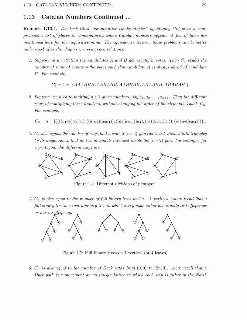
3. Cn also equals the number of ways that a convex (n+2)-gon cab be sub-divided into triangles
by its diagonals so that no two diagonals intersect inside the (n+2)-gon. For example, for
a pentagon, the different ways are
1
23
4
51
23
4
51
23
4
51
23
4
51
23
4
5
Figure 1.4: Different divisions of pentagon
4. Cn is also equal to the number of full binary trees on 2n + 1 vertices, where recall that a
full binary tree is a rooted binary tree in which every node either has exactly two offsprings
or has no offspring.
♥
♥
♥♥
♥♥
♥♥♥ ♥ ♥ ♥
♥♥
♥♥
♥♥♥ ♥
Figure 1.5: Full binary trees on 7 vertices (or 4 leaves)
5. Cn is also equal to the number of Dyck paths from (0, 0) to (2n, 0), where recall that a
Dyck path is a movement on an integer lattice in which each step is either in the North

40 CHAPTER 1. PROPERTIES OF INTEGERS AND BASIC COUNTING
East or in the South East direction (so the only movement from (0, 0) is either to (1, 1) or
to (1,−1)).
6. Cn also equals the number of n nonintersecting chords joining 2n points on the circumfer-
ence of a circle.
Figure 1.6: Non-intersecting chords using 6 points on the circle
7. Cn also equals the number of integer sequences that satisfy 1 ≤ a1 ≤ a2 ≤ · · · ≤ an and
ai ≤ i, for all i, 1 ≤ i ≤ n.
The following article has been taken from [2].
Let An denote the set of all lattice paths from (0, 0) to (n, n) and let Bn ⊂ An denote the set of
all lattice paths from (0, 0) to (n, n) that does not go above the line Y = X. Then, the numerical
values of |An| and |Bn| imply that (n+ 1) · |Bn| = |An|. The question arises:
can we find a partition of the set An into (n+1)-parts, say S0, S1, S2, . . . , Sn such that S0 = Bn
and |Si| = |S0|, for 1 ≤ i ≤ n?
The answer is in affirmative. Observe that any path from (0, 0) to (n, n) has n right moves.
So, the path is specified as soon as we know the successive right moves R1, R2, . . . , Rn, where
Ri equals ℓ if and only if Ri lies on the line Y = ℓ. For example, in Figure 1.3, R1 = 0, R2 =
0, R3 = 1, R4 = 1, . . . . These Ri’s satisfy
0 ≤ R1 ≤ R2 ≤ · · · ≤ Rn ≤ n. (1.1)
That is, any element of An can be represented by an ordered n-tuple (R1, R2, . . . , Rn) satisfying
Equation (1.1). Conversely, it can be easily verified that any ordered n-tuple (R1, R2, . . . , Rn)
satisfying Equation (1.1) corresponds to a lattice path from (0, 0) to (n, n). Note that, using
Remark 1.13.1.7, among the above n-tuples, the tuples that satisfy Ri ≤ i− 1, for 1 ≤ i ≤ n are
elements of Bn, and vice-versa. Now, we use the tuples that represent the elements of Bn to get
n+1 maps, f0, f1, . . . , fn, in such a way that fj(Bn) and fk(Bn) are disjoint, for 0 ≤ j 6= k ≤ n,
and An =n⋃
k=0
fk(Bn). In particular, for a fixed k, 0 ≤ k ≤ n, the map fk : Bn−→An is defined
by
fk((R1, R2, . . . , Rn)
)= (Ri1 ⊕n+1 k,Ri2 ⊕n+1 k, . . . , Rin ⊕n+1 k),
where ⊕n+1 denotes addition modulo n+ 1 and i1, i2, . . . , in is a rearrangement of the numbers
1, 2, . . . , n such that 0 ≤ Ri1 ⊕n+1 k ≤ Ri2 ⊕n+1 k ≤ · · · ≤ Rin ⊕n+1 k. The readers are advised
to prove the following exercise as they give the required partition of the set An.
1.14. GENERALIZATIONS 41
1.14 Generalizations
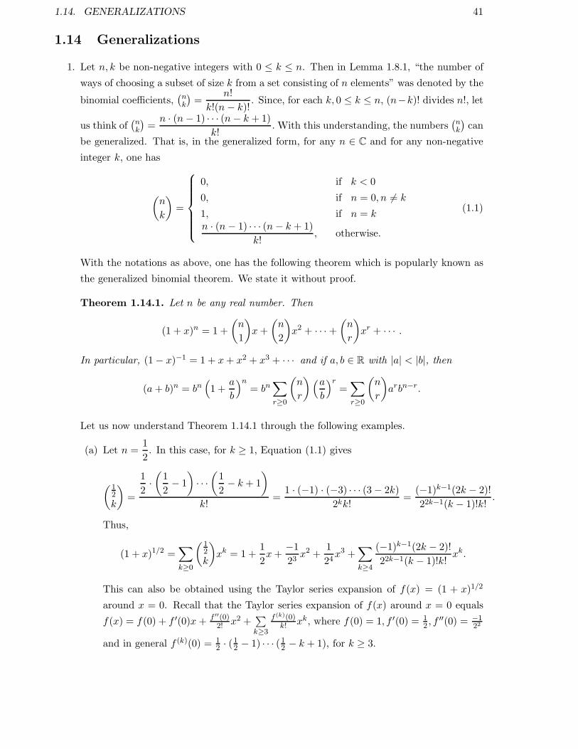
1. Let n, k be non-negative integers with 0 ≤ k ≤ n. Then in Lemma 1.8.1, “the number of
ways of choosing a subset of size k from a set consisting of n elements” was denoted by the
binomial coefficients,(nk
)=
n!
k!(n− k)!. Since, for each k, 0 ≤ k ≤ n, (n−k)! divides n!, let
us think of(nk
)=n · (n− 1) · · · (n− k + 1)
k!.With this understanding, the numbers
(nk
)can
be generalized. That is, in the generalized form, for any n ∈ C and for any non-negative
integer k, one has
(n
k
)
=
0, if k < 0
0, if n = 0, n 6= k
1, if n = kn · (n− 1) · · · (n− k + 1)
k!, otherwise.
(1.1)
With the notations as above, one has the following theorem which is popularly known as
the generalized binomial theorem. We state it without proof.
Theorem 1.14.1. Let n be any real number. Then
(1 + x)n = 1 +
(n
1
)
x+
(n
2
)
x2 + · · ·+(n
r
)
xr + · · · .
In particular, (1− x)−1 = 1 + x+ x2 + x3 + · · · and if a, b ∈ R with |a| < |b|, then
(a+ b)n = bn(
1 +a
b
)n= bn
∑
r≥0
(n
r
)(a
b
)r=∑
r≥0
(n
r
)
arbn−r.
Let us now understand Theorem 1.14.1 through the following examples.
(a) Let n =1
2. In this case, for k ≥ 1, Equation (1.1) gives
(12
k
)
=
1
2·(1
2− 1
)
· · ·(1
2− k + 1
)
k!=
1 · (−1) · (−3) · · · (3− 2k)
2kk!=
(−1)k−1(2k − 2)!
22k−1(k − 1)!k!.
Thus,
(1 + x)1/2 =∑
k≥0
(12
k
)
xk = 1 +1
2x+
−1
23x2 +
1
24x3 +
∑
k≥4
(−1)k−1(2k − 2)!
22k−1(k − 1)!k!xk.
This can also be obtained using the Taylor series expansion of f(x) = (1 + x)1/2
around x = 0. Recall that the Taylor series expansion of f(x) around x = 0 equals
f(x) = f(0) + f ′(0)x+ f ′′(0)2! x2 +
∑
k≥3
f(k)(0)k! xk, where f(0) = 1, f ′(0) = 1
2 , f′′(0) = −1
22
and in general f (k)(0) = 12 · (12 − 1) · · · (12 − k + 1), for k ≥ 3.

42 CHAPTER 1. PROPERTIES OF INTEGERS AND BASIC COUNTING
(b) Let n = −r, where r is a positive integer. Then, for k ≥ 1, Equation (1.1) gives
(−rk
)
=−r · (−r − 1) · · · (−r − k + 1)
k!= (−1)k
(r + k − 1
k
)
.
Thus,
(1 + x)n =1
(1 + x)r= 1− rx+
(r + 1
2
)
x2 +∑
k≥3
(r + k − 1
k
)
(−x)k.
The readers are advised to get the above expression using the Taylor series expansion
of (1 + x)n around x = 0.
2. Let n,m ∈ N. Recall the identity nm =m∑
k=0
(nk
)k!S(m,k) =
n∑
k=0
(nk
)k!S(m,k) that appeared
in Lemma 1.9.5 (see Equation (1.2)). We note that for a fixed positive integer m, the above
identity is same as the matrix product X = AY , where
X =
0m
1m
2m
3m
...
nm
, A =
(00
)0 0 0 · · · 0
(10
) (11
)0 0 · · · 0
(20
) (21
) (22
)0 · · · 0
(30
) (31
) (32
) (33
)· · · 0
......
......
. . ....
(n0
) (n1
) (n2
) (n3
)· · ·
(nn
)
and Y =
0!S(m, 0)
1!S(m, 1)
2!S(m, 2)...
n!S(m,n)
.
Hence, if we know the inverse of the matrix A, we can write Y = A−1X. Check that
A−1 =
(00
)0 0 0 · · · 0
−(10
) (11
)0 0 · · · 0
(20
)−(21
) (22
)0 · · · 0
−(30
) (31
)−(32
) (33
)· · · 0
......
......
. . ....
(−1)n(n0
)(−1)n−1
(n1
)(−1)n−2
(n2
)(−1)n−3
(n3
)· · ·
(nn
)
.
This gives us a way to calculate the Stirling numbers of second kind as a function of
binomial coefficients. That is, verify that
S(m,n) =1
n!
∑
k≥0
(−1)k(n
k
)
(n− k)m. (1.2)
The above ideas imply that for all non-negative integers n the identity
a(n) =∑
k≥0
(n
k
)
b(k) holds if and only if b(n) =∑
k≥0
(−1)k(n
k
)
a(k) holds.
1.14. GENERALIZATIONS 43
3. We end this chapter with an example which has a history (see [5]) of being solved by many
mathematicians such as Montmort, N. Bernoulli and de Moivre. We present the idea that
was proposed by Euler.
Example 1.14.2. On a rainy day, n students leave their umbrellas (which are indistin-
guishable) outside their examination room. Determine the number of ways of collecting the
umbrellas so that no student collects the correct umbrella when they finish the examination?
This problem is generally known by the Derangement problem.
Solution: Let the students be numbered 1, 2, . . . , n and suppose that the ith student has
the umbrella numbered i, 1 ≤ i ≤ n. So, we are interested in the number of permutations
of the set 1, 2, . . . , n such that the number i is not at the ith position, for 1 ≤ i ≤ n.
Let Dn represent the number of derangements. Then it can be checked that D2 = 1 and
D3 = 2. They correspond the permutations 21 for n = 2 and 231, 312 for n = 3. We will
try to find a relationship of Dn with Di, for 1 ≤ i ≤ n− 1.
Let us have a close look at the required permutations. We note that n should not be
placed at the nth position. So, n has to appear some where between 1 and n − 1. That
is, for some i, 1 ≤ i ≤ n− 1
(a) n appears at the ith position and i appears at the nth position, or
(b) n appears at the ith position and i does not appear at the nth position.
Case (a): Fix i, 1 ≤ i ≤ n − 1. Then the position of n and i is fixed and the remaining
numbers j, for j 6= i, n should not appear at the jth place. As j 6= i, n, the problem
reduces to the number of derangements of n − 2 numbers which by our notation equals
Dn−2. As i can be any one of the integers 1, 2, . . . , n − 1, the number of derangements
corresponding to the first case equals (n− 1)Dn−2.
Case (b): Fix i, 1 ≤ i ≤ n − 1. Then the position of n is at the ith place but i is not
placed at the nth position. So, in this case, the problem reduces to placing the numbers
1, 2, . . . , n− 1 at the places 1, 2, . . . , i− 1, i+ 1, . . . , n such that the number i is not to be
placed at the nth position and for j 6= i, j is not placed at the jth position. Let us rename
the positions as a1, a2, . . . , an−1, where ai = n and aj = j for j 6= i.
Then, with this renaming, the problem reduces to placing the numbers 1, 2, . . . , n − 1 at
places a1, a2, . . . , an−1 such that the number j, for 1 ≤ j ≤ n − 1, is not placed at aj ’th
position. This corresponds to the derangement of n− 1 numbers that this by our notation
equals Dn−1. Thus, in this case the number of derangements equals (n− 1)Dn−1.
Hence, Dn = (n − 1)Dn−1 + (n − 1)Dn−2. Or equivalently, D2 = 1 and D1 = 0 imply
Dn − nDn−1 = −(Dn−1 − (n − 1)Dn−2
)= (−1)2
(Dn−2 − (n − 2)Dn−3
)= · · · = (−1)n.

44 CHAPTER 1. PROPERTIES OF INTEGERS AND BASIC COUNTING
Therefore,
Dn = nDn−1 + (−1)n = n((n− 1)Dn−2 + (−1)n−1
)+ (−1)n
= n(n− 1)Dn−2 + n(−1)n−1 + (−1)n
...
= n(n− 1) · · · 4 · 3 D2 + n(n− 1) · · · 4(−1)3 + · · ·+ n(−1)n−1 + (−1)n
= n!
(
1 +−1
1!+
(−1)2
2!+ · · ·+ (−1)n−1
(n− 1)!+
(−1)n
n!
)
.
Or, in other words limn−→∞
Dn
n!=
1
e.
Notes: Most of the ideas for this chapter have come from the books [4], [7] and [8].

Chapter 2
Advanced Counting and Generating
Functions
2.1 Pigeonhole Principle
The pigeonhole principle states that if there are n + 1 pigeons and n holes (boxes), then there
is at least one hole (box) that contains two or more pigeons. It can be easily verified that the
pigeonhole principle is equivalent to the following statements:
1. If m pigeons are put into m pigeonholes, there is an empty hole if and only if there’s a
hole with more than one pigeon.
2. If n pigeons are put into m pigeonholes, with n > m, then there is a hole with more than
one pigeon.
3. For two finite sets A and B, there exists a one to one and onto function f : A −→ B if
and only if |A| = |B|.
Remark 2.1.1. Recall that the expression ⌈x⌉, called the ceiling function, is the smallest
integer ℓ, such that ℓ ≥ x and the expression ⌊x⌋, called the floor function, is the largest
integer k, such that k ≤ x.
1. [Generalized Pigeonhole Principle] if there are n pigeons and m holes with n > m,
then there is at least one hole that contains ⌈ nm⌉ pigeons.
2. Dirichlet was the one who popularized this principle.
Example 2.1.2. Let a be an irrational number. Then prove that there exist infinitely many
rational numbers s =p
q, such that |a− s| < 1
q2.
45

46 CHAPTER 2. ADVANCED COUNTING AND GENERATING FUNCTIONS
Proof. Let N ∈ N. Without loss of generality, we assume that a > 0. By α, we will denote
the fractional part of α. That is, α = α− ⌊α⌋.Now, consider the fractional parts 0, a, 2a, . . . , Na of the first (N + 1) multiples
of a and the N subintervals [0, 1N ), [ 1N ,
2N ), . . . , [N−1
N , 1) of [0, 1). Clearly ka, for k a positive
integer, cannot be an integer as a is an irrational number. Thus, by the pigeonhole principle,
two of the above fractional parts must fall into the same subinterval. That is, there exist integers
u, v and w such that u > v but
ua ∈ [w
N,w + 1
N) and va ∈ [
w
N,w + 1
N).
Thus, |ua − va| < 1
Nand |ua − va| = |(u − v)a − (⌊ua⌋ − ⌊va⌋)|. Now, let q = u − v
and p = ⌊ua⌋ − ⌊va⌋. Then p, q ∈ Z, q 6= 0 and |qa− p| < 1N . Dividing by q, we get
|a− p
q| < 1
Nq≤ 1
q2as 0 < q ≤ N.
Therefore, we have found a rational numberp
qsuch that |a− p
q| < 1
q2. We will now show that
the number of such pairs (p, q) is infinite.
On the contrary, assume that there are only a finite number of rational numbers, say
r1, r2, . . . , rM such that
ri =piqi, for i = 1, . . . ,M, and |a− ri| <
1
q2i.
Since a is an irrational number, none of the differences |a−ri|, for i = 1, 2, . . . ,M , will be exactly
0. Therefore, there exists an integer Q such that
|a− ri| >1
Q, for all i = 1, 2, . . . ,M.
We now, apply our earlier argument to this Q. The argument gives the existence of a fraction
r =p
qsuch that |a−r| < 1
Qq <1Q < |a−ri|, for 1 ≤ i ≤M . Hence, r 6= ri, for all i = 1, 2, . . . ,M.
On the other hand, we also have, |a− r| < 1
q2contradicting the assumption that the fractions
ri, for i = 1, 2, . . . ,M , were all the fractions with this property.

2.2. PIGEONHOLE PRINCIPLE CONTINUED ... 47
2.2 Pigeonhole Principle Continued ...
Example 2.2.1. 1. Let a1, a2, . . . , amn+1 be a sequence of distinct mn + 1 real numbers.
Then prove that this sequence has a subsequence of either (m+ 1) numbers that is strictly
increasing or (n+ 1) numbers that is strictly decreasing.
Observation: The statement is NOT TRUE if there are exactly mn numbers. For ex-
ample, consider the sequence 4, 3, 2, 1, 8, 7, 6, 5, 12, 11, 10, 9 of 12 = 3× 4 distinct numbers.
This sequence neither has an increasing subsequence of 4 numbers nor a decreasing subse-
quence of 5 numbers. Also, observe that if we take any number different from 1, 2, . . . , 12
and place it at any position in the above sequence then it can be verified that there is either
an increasing subsequence of 4 numbers or a decreasing subsequence of 5 numbers. For
example, if we place 7.5,
(a) “before the number 4” or “between the numbers 8 and 7” or “after the number 9”,
then there is a decreasing subsequence of length 5.
(b) “between the numbers 4 and 8” or between the numbers 7 and 9, then there is an
increasing subsequence of length 4.
Proof. Let T be the given sequence. That is, T = akmn+1k=1 and define
ℓi = maxs
s : an increasing subsequence of length s exists starting with ai.
Then there aremn+1 positive integers ℓ1, ℓ2, . . . , ℓmn+1. If there exists a j, 1 ≤ j ≤ mn+1,
such that ℓj ≥ m+1, then by definition of ℓj, there exists an increasing sequence of length
m+1 starting with aj and thus the result follows. So, on the contrary assume that ℓi ≤ m,
for 1 ≤ i ≤ mn+ 1.
That is, we have mn + 1 numbers (ℓ1, . . . , ℓmn+1) and all of them have to be put in the
boxes numbered 1, 2, . . . ,m. So, by the generalized pigeonhole principle, there are at least⌈mn+ 1
m
⌉
= n+1 numbers (ℓi’s) that lies in the same box. Therefore, let us assume that
there exist numbers 1 ≤ i1 < i2 < · · · < in+1 ≤ mn+ 1, such that
ℓi1 = ℓi2 = · · · = ℓin+1 . (2.1)
That is, the length of the largest increasing subsequences of T starting with the numbers
ai1 , ai2 , . . . , ain+1 are all equal. We now claim that ai1 > ai2 > · · · > ain+1 .
We will show that ai1 > ai2 . A similar argument will give the other inequalities and hence
the proof of the claim. On the contrary, let if possible ai1 < ai2 (recall that ai’s are
distinct) and consider a largest increasing subsequence ai2 = α1 < α2 < · · · < αi2 of T ,
starting with ai2 , that has length ℓi2 . This subsequence with the assumption that ai1 < ai2
gives an increasing subsequence
ai1 < ai2 = α1 < α2 < · · · < αℓi2

48 CHAPTER 2. ADVANCED COUNTING AND GENERATING FUNCTIONS
of T , starting with ai1 , of length ℓi2 +1. So, by definition of ℓi’s, ℓi1 ≥ ℓi2 +1. This gives a
contradiction to the equality, ℓi1 = ℓi2 , in Equation (2.1). Hence the proof of the example
is complete.
2. Prove that there exist two powers of 3 whose difference is divisible by 2011.
Proof. Consider the set S = 1 = 30, 3, 32, 33, . . . , 32011. Then |S| = 2012. Also, we
know that when we divide positive integers by 2011 then the possible remainders are
0, 1, 2, . . . , 2010 (corresponding to exactly 2011 boxes). So, if we divide the numbers in S
with 2011, then by pigeonhole principle there will exist at least two numbers 0 ≤ i < j ≤2011, such that the remainders of 3j and 3i, when divided by 2011, are equal. That is,
2011 divides 3j − 3i. Hence, this completes the proof.
Observe that this argument also implies that “there exists a positive integer ℓ such that
2011 divides 3ℓ − 1” or “there exists a positive power of 3 that leaves a remainder 1 when
divided by 2011” as gcd(3, 2011) = 1.
3. Prove that there exists a power of three that ends with 0001.
Proof. Consider the set S = 1 = 30, 3, 32, 33, . . .. Now, let us divide each element of
S by 104. As |S| > 104, there exist i > j such that the remainders of 3i and 3j , when
are divided by 104, are equal. But gcd(104, 3) = 1 and thus, 104 divides 3ℓ − 1. That is,
3ℓ − 1 = s · 104 for some positive integer s. That is, 3ℓ = s · 104 + 1 and hence the result
follows.

2.3. PRINCIPLE OF INCLUSION AND EXCLUSION 49
2.3 Principle of Inclusion and Exclusion
The following result is well known and hence we omit the proof.
Theorem 2.3.1. Let U be a finite set. Suppose A and B are two subsets of U . Then the number
of elements of U that are neither in A nor in B are
|U | −(|A|+ |B| − |A ∩B|
).
Or equivalently, |A ∪B| = |A|+ |B| − |A ∩B|.
A generalization of this to three subsets A,B and C is also well known. To get a result that
generalizes Theorem 2.3.1 for n subsets A1, A2, . . . , An, we need the following notations:
S1 =n∑
i=1
|Ai|, S2 =∑
1≤i<j≤n
|Ai∩Aj |, S3 =∑
1≤i<j<k≤n
|Ai∩Aj∩Ak|, · · · , Sn = |A1∩A2∩· · ·∩An|.
With the notations as defined above, we have the following theorem, called the inclusion-
exclusion principle. This theorem can be easily proven using the principle of mathematical
induction. But we give a separate proof for better understanding.
Theorem 2.3.2. [Inclusion-Exclusion Principle] Let A1, A2, . . . , An be n subsets of a finite set
U . Then the number of elements of U that are in none of A1, A2, . . . , An is given by
|U | − S1 + S2 − S3 + · · ·+ (−1)nSn. (2.1)
Or equivalently,
|A1 ∪A2 ∪ · · · ∪An| = S1 − S2 + · · · + (−1)n−1Sn. (2.2)
Proof. We show that if an element x ∈ U belongs to exactly k of the subsets A1, A2, . . . , An,
for some k ≥ 1, then its contribution in (2.1) is zero. Suppose x belongs to exactly k subsets
Ai1 , Ai2 , . . . , Aik . Then we observe the following:
1. The contribution of x in |U | is 1.
2. The contribution of x in S1 is k as x ∈ Aij , 1 ≤ j ≤ k.
3. The contribution of x in S2 is(k2
)as x ∈ Aij ∩Ail , 1 ≤ j < l ≤ k.
4. The contribution of x in S3 is(k3
)as x ∈ Aij ∩Ail ∩Aim , 1 ≤ j < l < m ≤ k.
Proceeding this way, we have
5. The contribution of x in Sk is(kk
)= 1, and
6. The contribution of x in Sℓ for ℓ ≥ k + 1 is 0.

50 CHAPTER 2. ADVANCED COUNTING AND GENERATING FUNCTIONS
So, the contribution of x in (2.1) is
1− k +
(k
2
)
−(k
3
)
+ · · ·+ (−1)k−1
(k
k − 1
)
+ (−1)k(k
k
)
+ 0 · · · + 0 = (1− 1)k = 0.
This completes the proof of the theorem. The readers are advised to prove the equivalent
condition.
Example 2.3.3. 1. Determine the number of 10-letter words using ENGLISH alphabets that
does not contain all the vowels.
Solution: Let U be the set consisting of all the 10-letters words using ENGLISH alphabets
and let Aα be a subset of U that does not contain the letter α. Then we need to compute
|Aa ∪Ae ∪Ai ∪Ao ∪Au| = S1 − S2 + S3 − S4 + S5,
where S1 =∑
α∈a,e,i,o,u
|Aα| =(51
)2510, S2 =
(52
)2410, S3 =
(53
)2310, S4 =
(54
)2210 and
S5 = 2110. So, the required answer is5∑
k=1
(−1)k−1(5k
)(26− k)10.
2. Determine the number of integers between 1 and 1000 that are coprime to 2, 3, 11 and 13.
Solution: Let U = 1, 2, 3, . . . , 1000 and let Ai = n ∈ U : i divides n, for i =
2, 3, 11, 13. Then note that we need the value of |U | − |A2 ∪ A3 ∪ A11 ∪ A13|. Observe
that
|A2| = ⌊10002
⌋ = 500, |A3| = ⌊10003
⌋ = 333, |A11| = ⌊100011
⌋ = 90, |A13| = ⌊100013
⌋ = 76,
|A2 ∩A3| = ⌊10006
⌋ = 166, |A2 ∩A11| = ⌊100022
⌋ = 45, |A2 ∩A13| = ⌊100026
⌋ = 38,
|A3 ∩A11| = ⌊100033
⌋ = 30, |A3 ∩A13| = ⌊100039
⌋ = 25, |A11 ∩A13| = ⌊1000143
⌋ = 6,
|A2 ∩A3 ∩A11| = 15, |A2 ∩A3 ∩A13| = 12, |A2 ∩A11 ∩A13| = 3,
|A3 ∩A11 ∩A13| = 2, |A2 ∩A3 ∩A11 ∩A13| = 1.
Thus, the required number is
1000−((500+333+90+76)−(166+45+38+30+25+6)−(15+12+3+2)−1
)= 1000−720 = 280.
3. (Euler’s φ-function Or Euler’s totient function) Let n denote a positive integer.Then the
Euler φ-function is defined by
φ(n) =∣∣k : 1 ≤ k ≤ n, gcd(n, k) = 1
∣∣. (2.3)
Determine a formula for φ(n) in terms of its prime factors.
Solution: Let n = pα11 pα2
2 · · · pαkk be the unique decomposition of n as product of distinct
2.3. PRINCIPLE OF INCLUSION AND EXCLUSION 51
primes p1, p2, . . . , pk, U = 1, 2, . . . , n and let Api = m ∈ U : pi divides m, for 1 ≤ i ≤k. Then, by definition
φ(n) = |U | − S1 + S2 − S3 + · · ·+ (−1)kSk
= n−k∑
i=1
n
pi+
∑
1≤i<j≤k
n
pipj− · · ·+ (−1)k
n
p1p2 · · · pk
= n
k∏
i=1
(
1− 1
pi
)
. (2.4)

52 CHAPTER 2. ADVANCED COUNTING AND GENERATING FUNCTIONS
2.4 Formal Power Series
In this chapter, we will first try to develop the theory of generating functions by getting closed
form expressions for some known recurrence relations. These ideas will be used later to get some
binomial identities.
To do so, we first recall from Page 41 that for all n ∈ Q and k ∈ Z, k ≥ 0, the binomial
coefficients,(nk
), are well defined, using the idea that
(nk
)=n(n− 1)(n − 2) · · · (n − k + 1)
k!. We
now start with the definition of “formal power series” over Q and study its properties in some
detail.
Definition 2.4.1 (Formal power series). An algebraic expression of the form f(x) =∑
n≥0anx
n,
where an ∈ Q for all n ≥ 0, is called a formal power series in the indeterminate x over Q.
The set of all formal power series in the indeterminate x, with coefficients from Q will be
denoted by P(x).
Remark 2.4.2. 1. Given a sequence of numbers an ∈ Q : n = 0, 1, 2, . . ., one associates
two formal power series, namely,∑
n≥0anx
n and∑
n≥0anxn
n!. The expression
∑
n≥0anx
n is called
the generating function and the expression∑
n≥0anxn
n!is called the exponential generating
function, for the numbers an : n ≥ 0.
2. Let f(x) =∑
n≥0anx
n be a formal power series. Then the coefficient of xn, for n ≥ 0, in
f(x) is denoted by [xn]f(x). That is, a0 = [x0]f(x) and an = [xn]f(x), for n ≥ 1.
3. One thinks of∑
n≥0anx
n as an algebraic expression. In general, one is interested only in
computing the coefficient of certain power of x and not in evaluating them for any value
of x. But, if at all there is a need to evaluate it at a point, say x0, then one needs to
determine its “radius of convergence” and then evaluate it if x0 lies within that radius.
We need the following definition to proceed further.
Definition 2.4.3 (Equality of two formal power series). Two elements f(x) =∑
n≥0anx
n and
g(x) =∑
n≥0bnx
n of P(x) are said to be equal if an = bn, for all n ≥ 0.
We are now ready to define the algebraic rules:
Definition 2.4.4. Let f(x) =∑
n≥0anx
n, g(x) =∑
n≥0bnx
n ∈ P(x). Then their
1. sum/addition is defined by
f(x) + g(x) =∑
n≥0
anxn +
∑
n≥0
bnxn =
∑
n≥0
(an + bn)xn.

2.4. FORMAL POWER SERIES 53
2. product is defined by
f(x) ·g(x) =
∑
n≥0
anxn
·
∑
n≥0
bnxn
=∑
n≥0
cnxn, where cn =
n∑
k=0
akbn−k, for n ≥ 0.
This product is also called the Cauchy product.
Remark 2.4.5. 1. In case of exponential power series, the product of f(x) =∑
n≥0anxn
n!and
g(x) =∑
n≥0bnxn
n!equals
∑
n≥0dnxn
n!, where dn =
n∑
k=0
(nk
)akbn−k, for n ≥ 0.
2. Note that the expression eex−1 is a well defined formal power series as the definition ey =
∑
n≥0
yn
n!implies that ee
x−1 =∑
n≥0
(ex − 1)n
n!and hence
[xm]eex−1 = [xm]
∑
n≥0
(ex − 1)n
n!=
m∑
n=0
[xm](ex − 1)n
n!. (2.1)
That is, for each m ≥ 0, [xm]eex−1 is a sum of a finite number of real numbers. Where
as the expression eexis not a formal power series as the computation of [xm]ee
x, for all
m ≥ 0, will indeed require an infinite sum.
Thus, under the algebraic operations defined above, it can be checked that the set P(x) forms
a Commutative Ring with identity, where the identity element is given by the formal power series
f(x) = 1. In this ring, the element f(x) =∑
n≥0anx
n is said to have a reciprocal if there exists
another element g(x) =∑
n≥0bnx
n ∈ P(x) such that f(x) ·g(x) = 1. So, the question arises, under
what conditions on the coefficients of f(x), can we find g(x) ∈ P(x) such that f(x)g(x) = 1.
The answer to this question is given in the following proposition.
Proposition 2.4.6. Let f(x) =∑
n≥0anx
n ∈ P(x). Then there exists g(x) ∈ P(x) satisfying
f(x) · g(x) = 1 if and only if a0 6= 0.
Proof. Let g(x) =∑
n≥0bnx
n ∈ P(x). Then, by the definition of Cauchy product, f(x)g(x) =
∑
n≥0cnx
n, where cn =n∑
k=0
akbn−k, for all n ≥ 0. Therefore, using the definition of equality of two
power series, we see that f(x)g(x) = 1 if and only if c0 = 1 and cn = 0, for all n ≥ 1.
Therefore, if a0 = 0 then c0 = 0 and hence the Cauchy product f(x)g(x) can never equal 1.
However, if a0 6= 0, then the coefficients bn’s can be recursively obtained as follows:
b0 =1
a0as 1 = c0 = a0b0.
b1 =−1
a0· (a1b0) as 0 = c1 = a0b1 + a1b0.

54 CHAPTER 2. ADVANCED COUNTING AND GENERATING FUNCTIONS
b2 =−1
a0· (a2b0 + a1b1) as 0 = c2 = a0b2 + a1b1 + a2b0. And in general, if we have already
computed the values of bk, for k ≤ r, then
br+1 =−1
a0· (ar+1b0 + arb1 + · · ·+ a1br) as 0 = cr+1 = ar+1b0 + arb1 + · · ·+ a1br + a0br+1.
Note that if the coefficients an’s come from R, a commutative ring with unity, then one needs
b0 to be an invertible element of R for Proposition 2.4.6 to hold true. Let us now look at the
composition of two formal power series. Recall that, if f(x) =∑
n≥0anx
n, g(x) =∑
n≥0bnx
n ∈ P(x)
then the composition (f g)(x) = f(g(x)) =∑
n≥0an(g(x))
n =∑
n≥0an(
∑
m≥0bmx
m)n may not be
defined (just to compute the constant term of the composition, one may have to look at an
infinite sum). For example, let f(x) = ex and g(x) = x + 1. Note that g(0) = 1 6= 0. Here,
(f g)(x) = f(g(x)) = f(x + 1) = ex+1. So, as function f g is well defined, but there is no
formal procedure to write ex+1 as∑
k≥0
akxk ∈ P(x) (i.e., with ak ∈ Q) and hence ex+1 is not a
formal power series over Q.
The next result gives the condition under which the composition (f g)(x) is well defined.
Proposition 2.4.7. Let f(x) =∑
n≥0anx
n and g(x) =∑
n≥0bnx
n be two formal power series. Then
the composition (f g)(x) is well defined if either f is a polynomial or b0 = 0.
Moreover, suppose that a0 = 0. Then, there exists g(x) =∑
n≥0bnx
n, with b0 = 0, such that
(f g)(x) = x. Furthermore, (g f)(x) is well defined and (g f)(x) = x.
Proof. Let (f g)(x) = f(g(x)) =∑
n≥0cnx
n and suppose that either f is a polynomial or
b0 = 0. Then to compute ck = [xk] (f g)(x), for k ≥ 0, one just needs to consider the terms
a0 + a1g(x) + a2(g(x))2 + · · ·+ ak(g(x))
k. Hence, each ck is a real number and (f g)(x) is welldefined. This completes the proof of the first portion. The proof of the other part is left to the
readers.
We now define the formal differentiation of elements of P(x) and state a result without proof.
Definition 2.4.8 (Differentiation). Let f(x) =∑
n≥0anx
n ∈ P(x). Then the formal differentia-
tion of f(x), denoted Df(x), is defined by
Df(x) = a1 + 2a2x+ · · ·+ nanxn−1 + · · · =
∑
n≥1
nanxn−1.
Proposition 2.4.9. Let f(x) =∑
n≥0anx
n ∈ P(x). Then f(x) = a0, a constant, whenever
Df(x) = 0. Also, f(x) = a0ex whenever Df(x) = f(x).

2.5. FORMAL POWER SERIES CONTINUED ... 55
2.5 Formal Power Series Continued ...
Before proceeding further, let us look at some important examples, where the above results can
be used.
Example 2.5.1. Using the generalized binomial theorem (see Theorem 1.14.1), recall that, for
a positive integer r, the formal power series
∑
n≥0
(n+ r − 1
n
)
xn equals1
(1− x)r. (2.1)
In particular, for r = 1, the formal power series∑
n≥0xn equals
1
1− x.
1. Determine a closed form expression for∑
n≥0nxn ∈ P(x).
Solution: As1
1− x=∑
n≥0xn, one has
1
(1− x)2= D
(1
1− x
)
= D
(
∑
n≥0xn
)
=∑
n≥0nxn−1.
Thus, the closed form expression isx
(1− x)2.
This can also be computed as follows:
Let S =∑
n≥0nxn = x + 2x2 + 3x3 + · · · . Then xS = x2 + 2x3 + 3x4 + · · · . Hence,
(1− x)S = x+ x2 + x3 + · · · = x(1 + x+ x2 + · · · ) = x
1− x. Thus, S =
x
(1− x)2.
2. Let f(x) =∑
n≥0anx
n ∈ P(x). Determinen∑
k=0
ak.
Solution: Recall that the Cauchy product of f(x) =∑
n≥0anx
n and g(x) =∑
n≥0bnx
n equals
∑
n≥0cnx
n, where cn =n∑
k=0
akbn−k, for n ≥ 0. Therefore, to get cn =n∑
k=0
ak, one needs
bk = 1, for all k ≥ 0. That is,n∑
k=0
ak = cn = [xn]
(
f(x) · 1
1− x
)
.
Hence, the Cauchy product helps us in computing the sum of the first N coefficients of a
formal power series, for any N ≥ 1.
3. Determine the sum of the squares of the first N positive integers.
Solution: Using Equation (2.1), observe that k = [xk−1]
(1
(1− x)2
)
. Therefore, using
Example 2.5.1.2, one has
N∑
k=1
k = [xN−1]
(1
(1− x)2· 1
1− x
)
= [xN−1]1
(1− x)3=
(N − 1 + 3− 1
N − 1
)
=N(N + 1)
2.
4. Determine a closed form expression forN∑
k=1
k2.
Solution: Using Example 2.5.1.1, observe that∑
k≥0
kxk =x
(1− x)2. Therefore, using the

56 CHAPTER 2. ADVANCED COUNTING AND GENERATING FUNCTIONS
differentiation operator, one obtains
∑
k≥0
k2xk = x
∑
k≥0
k2xk−1
= xD
(x
(1 − x)2
)
=x(1 + x)
(1− x)3. (2.2)
Thus, by Example 2.5.1.2
N∑
k=1
k2 = [xN ]
(x(1 + x)
(1− x)3· 1
1− x
)
= [xN−1]
(1
(1− x)4
)
+ [xN−2]
(1
(1− x)4
)
=
(N − 1 + 4− 1
N − 1
)
+
(N − 2 + 4− 1
N − 2
)
=N(N + 1)(2N + 1)
6.
5. Determine a closed form expression forN∑
k=1
k3.
Solution: Using Equation (2.2), observe that∑
k≥0
k2xk =x(1 + x)
(1− x)3. So,
∑
k≥0
k3xk = x
∑
k≥0
k3xk−1
= xD
(x(1 + x)
(1 − x)3
)
=x(1 + 4x+ x2)
(1− x)4.
Thus, by Example 2.5.1.2
N∑
k=1
k3 = [xN ]
(x(1 + 4x+ x2
(1− x)4)· 1
1− x
)
= [xN−1]
(1
(1− x)5
)
+ [xN−2]
(4
(1− x)5
)
+ [xN−3]
(1
(1− x)5
)
=
(N − 1 + 5− 1
N − 1
)
+ 4
(N − 2 + 5− 1
N − 2
)
+
(N − 3 + 5− 1
N − 3
)
=
(N(N + 1)
2
)2
.
Hence, we observe that we can inductively use this technique to get a closed form expression
forN∑
k=1
kr, for any positive integer r.
6. Determine a closed form expression for∑
n≥0
n2 + n+ 6
n!.
Solution: As we need to compute the infinite sum, Cauchy product cannot be used. Also,
one needs to find a convergent series, which when evaluated at some x0, gives the required
expression. Therefore, recall that the series ex =∑
n≥0
xn
n!, converges for all x ∈ R and
evaluating ex at x = 1, gives∑
n≥0
1
n!= e. Similarly,
n
n!= [xn] (xD(ex)) = [xn] (xex) and
2.5. FORMAL POWER SERIES CONTINUED ... 57
n2
n!= [xn] (xD(xDex)) = [xn]
((x+ x2)ex
). Thus,
∑
n≥0
n2 + n+ 6
n!= (x+ x2)ex + xex + 6ex
∣∣∣∣x=1
= 9e.
7. Let n and r be two fixed positive integers. Then determine the number of non-negative
integer solutions to the system x1 + x2 + · · ·+ xn = r.
Solution: Recall that this number equals(r+n−1
r
)(see Lemma 1.10.2).
In this chapter, we can think of the problem as follows: the above system can be interpreted
as coming from the monomial xr, where r = x1+x2+ · · ·+xn. That is, the problem reduces
to finding the coefficients of yxk of a formal power series, for non-negative integers xk’s.
Now, recall that the terms yxk appear with a coefficient 1 in the expression1
1− y=∑
i≥0yi.
Hence, the question reduces to computing
[yr]
(1
(1− y)(1− y) · · · (1− y)
)
= [yr]1
(1− y)n=
(r + n− 1
r
)
.
We now look at some examples that may require the use of the package “MATHEMATICA”
or “MAPLE” or ... to obtain the exact answer. So, in the examples given below, one is interested
in getting only a formal power series whose coefficient gives the required result even though it
may be difficult to compute the coefficient.
Example 2.5.2. 1. For fixed positive integers n and r, determine the number of non-negative
integer solutions to the system x1 + 2x2 + · · ·+ nxn = r.
Solution: The ideas from Example 2.5.1.7 imply that one needs to consider the formal
power series∑
i≥0xki =
1
1− xk. Hence, need to compute
[xr]1
(1− x)(1− x2) · · · (1− xn).
2. Determine the number of solutions to the system x1 + x2 + · · · + x5 = n, where xi’s are
non-negative integer, x1 ≥ 4, x4 ≤ 10 and xr is a multiple of r, whenever r 6= 1, 4.
Solution: The condition x1 ≥ 4 corresponds to looking at xk, for k ≥ 4, which corresponds
to the formal power series∑
k≥4
xk. Similarly, x4 ≤ 10 gives the formal power series10∑
k=0
xk
and the condition xr is a multiple of r, for r 6= 1, 4, corresponds to∑
k≥0
xrk. So, we need
to compute the coefficient of xn in the product
∑
k≥4
xk
·(
10∑
k=0
xk
)
·
∑
k≥0
x2k
·
∑
k≥0
x3k
·
∑
k≥0
x5k
=x4(1− x11)
(1− x)2(1− x2)(1− x3)(1− x5).

58 CHAPTER 2. ADVANCED COUNTING AND GENERATING FUNCTIONS
3. Determine the number of ways in which 100 voters can cast their 100 votes for 10 candi-
dates such that no candidate gets more than 20 votes.
Solution: Note that we are assuming that the voters are identical. So, we need to solve the
system in non-negative integers to the system x1 + x2 + · · ·+ x10 = 100, with 0 ≤ xi ≤ 20,
for 1 ≤ i ≤ 10. So, we need to find the coefficient of x100 in
(20∑
k=1
xk
)10
=(1 − x21)10
(1− x)10=
(10∑
i=0
(−1)i(10
i
)
x21i
)
·
∑
j≥0
(10 + j − 1
j
)
xj
.
Thus, the required answer equals [x100]
(20∑
k=1
xk)10
=4∑
i=0(−1)i
(10i
)·(109−21i
9
).
Before moving to the applications of formal power series to the solution of recurrence rela-
tions, let us list a few well known power series. The readers are requested to get a proof for
their satisfaction.Table of Formal Power Series
ex =∑
k≥0
xk
k!log(1− x) = − ∑
k≥1
xk
k, |x| < 1
(1 + x)a =∑
r≥0
(ak
)xk, |x| < 1
1
1− x=
∑
k≥0
xk, |x| < 1
1
(1− x)a=
∑
k≥0
(a+k−1
k
)xk, |x| < 1
1√1− 4x
=∑
k≥0
(2kk
)xk, |x| < 1
4
x−r(1 + x)n =∑
k≥−r
( nr+k
)xk, |x| < 1
xn
(1− x)n+1=
∑
k≥0
(kn
)xk, n ≥ 0, |x| < 1
sin(x) =∑
r≥0
(−1)rx2r+1
(2r + 1)!cos(x) =
∑
r≥0
(−1)rx2r
(2r)!
sinh(x) =∑
r≥0
x2r+1
(2r + 1)!cosh(x) =
∑
r≥0
x2r
(2r)!
1−√1− 4x
2x=∑
k≥0
1
k + 1
(2kk
)xk, |x| < 1
4
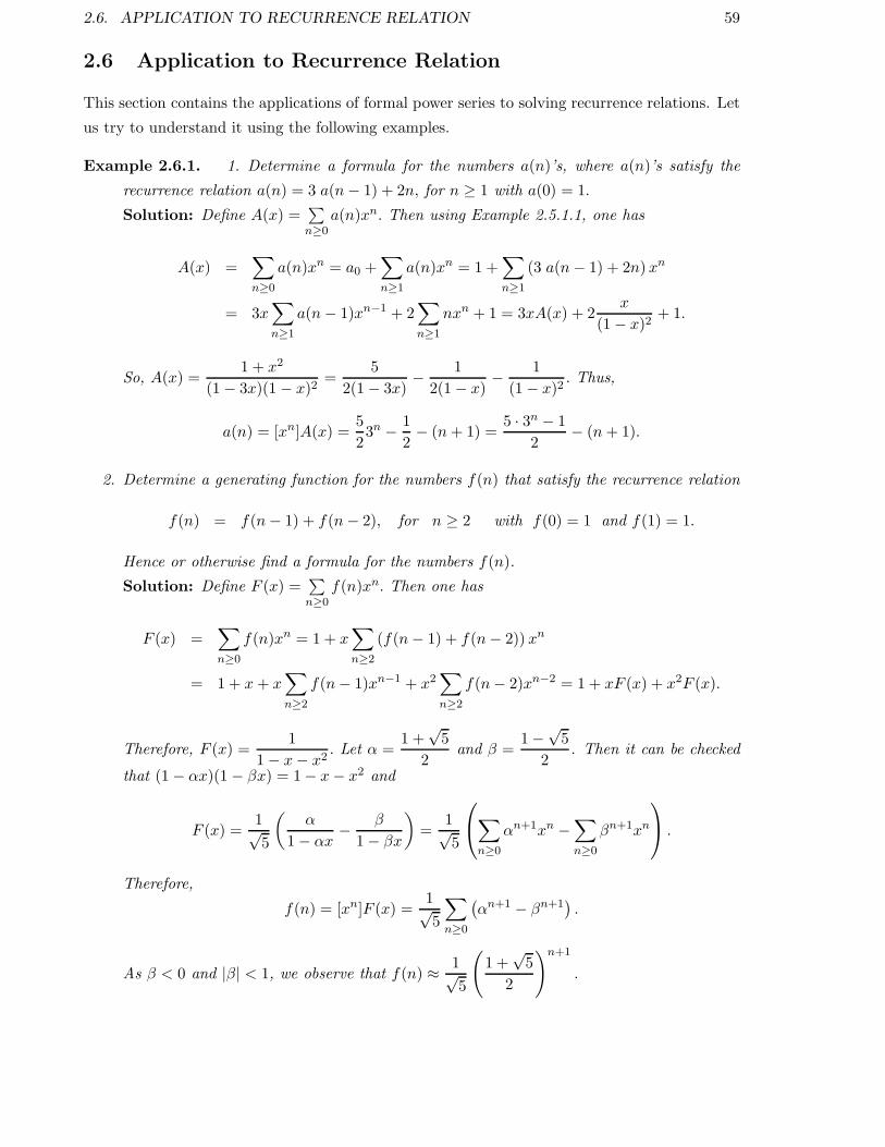
2.6. APPLICATION TO RECURRENCE RELATION 59
2.6 Application to Recurrence Relation
This section contains the applications of formal power series to solving recurrence relations. Let
us try to understand it using the following examples.
Example 2.6.1. 1. Determine a formula for the numbers a(n)’s, where a(n)’s satisfy the
recurrence relation a(n) = 3 a(n− 1) + 2n, for n ≥ 1 with a(0) = 1.
Solution: Define A(x) =∑
n≥0a(n)xn. Then using Example 2.5.1.1, one has
A(x) =∑
n≥0
a(n)xn = a0 +∑
n≥1
a(n)xn = 1 +∑
n≥1
(3 a(n− 1) + 2n) xn
= 3x∑
n≥1
a(n− 1)xn−1 + 2∑
n≥1
nxn + 1 = 3xA(x) + 2x
(1− x)2+ 1.
So, A(x) =1 + x2
(1− 3x)(1 − x)2=
5
2(1− 3x)− 1
2(1− x)− 1
(1− x)2. Thus,
a(n) = [xn]A(x) =5
23n − 1
2− (n+ 1) =
5 · 3n − 1
2− (n+ 1).
2. Determine a generating function for the numbers f(n) that satisfy the recurrence relation
f(n) = f(n− 1) + f(n− 2), for n ≥ 2 with f(0) = 1 and f(1) = 1.
Hence or otherwise find a formula for the numbers f(n).
Solution: Define F (x) =∑
n≥0f(n)xn. Then one has
F (x) =∑
n≥0
f(n)xn = 1 + x∑
n≥2
(f(n− 1) + f(n− 2)) xn
= 1 + x+ x∑
n≥2
f(n− 1)xn−1 + x2∑
n≥2
f(n− 2)xn−2 = 1 + xF (x) + x2F (x).
Therefore, F (x) =1
1− x− x2. Let α =
1 +√5
2and β =
1−√5
2. Then it can be checked
that (1− αx)(1 − βx) = 1− x− x2 and
F (x) =1√5
(α
1− αx− β
1− βx
)
=1√5
∑
n≥0
αn+1xn −∑
n≥0
βn+1xn
.
Therefore,
f(n) = [xn]F (x) =1√5
∑
n≥0
(αn+1 − βn+1
).
As β < 0 and |β| < 1, we observe that f(n) ≈ 1√5
(
1 +√5
2
)n+1
.

60 CHAPTER 2. ADVANCED COUNTING AND GENERATING FUNCTIONS
Remark 2.6.2. The numbers f(n), for n ≥ 0 are called Fibonacci numbers. It is
related with the following problem: Suppose a couple bought a pair of rabbits (each one
year old) in the year 2001. If a pair of rabbits starts giving birth to a pair of rabbits as
soon as they grow 2 years old, determine the number of rabbits the couple will have in the
year 2025.
3. Determine a formula for the numbers a(n)’s, where a(n)’s satisfy the recurrence relation
a(n) = 3 a(n− 1) + 4a(n− 2), for n ≥ 2 with a(0) = 1 and a(1) = c, a constant.
Solution: Define A(x) =∑
n≥0a(n)xn. Then
A(x) =∑
n≥0
a(n)xn = a0 + a1x+∑
n≥2
a(n)xn = 1 + cx+∑
n≥2
(3 a(n − 1) + 4 a(n− 2)) xn
= 1 + cx+ 3x∑
n≥2
a(n− 1)xn−1 + 4x2∑
n≥2
an−2xn−2
= 1 + cx+ 3x(A(x) − a0) + 4x2A(x).
So, A(x) =1 + (c− 3)x
(1− 3x− 4x2)=
1 + (c− 3)x
(1 + x)(1− 4x).
(a) If c = 4 then A(x) =1
1− 4xand hence an = [xn] A(x) = 4n.
(b) If c 6= 4 then A(x) =1 + c
5· 1
1− 4x+
4− c
5· 1
1 + xand hence
an = [xn] A(x) =(1 + c) 4n
5+
(−1)n(4− c)
5.
4. Determine a sequence, a(n) ∈ R : n ≥ 0, such that a0 = 1 andn∑
k=0
a(k)a(n−k) =(n+2
2
),
for all n ≥ 1.
Solution: Define A(x) =∑
n≥0a(n)xn. Then, using the Cauchy product, one has
A(x)2 =∑
n≥0
(n∑
k=0
a(k)a(n − k)
)
xn =∑
n≥0
(n+ 2
2
)
xn =1
(1− x)3.
Hence, A(x) = 1(1−x)3/2
and thus a(n) = (−1)n(−3/2
n
)=
3 · 5 · 7 · · · (2n+ 1)
2n n!, for all n ≥ 1.
5. Determine a generating function for the numbers f(n,m), n,m ∈ Z, n,m ≥ 0 that satisfy
f(n,m) = f(n− 1,m) + f(n− 1,m− 1), (n,m) 6= (0, 0) with (2.1)
f(n, 0) = 1, for all n ≥ 0 and f(0,m) = 0, for all m > 0.
Hence or otherwise, find a formula for the numbers f(n,m).
Solution: Note that in the above recurrence relation, the value of m need not be ≤ n.
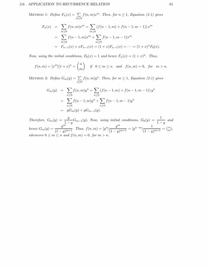
2.6. APPLICATION TO RECURRENCE RELATION 61
Method 1: Define Fn(x) =∑
m≥0f(n,m)xm. Then, for n ≥ 1, Equation (2.1) gives
Fn(x) =∑
m≥0
f(n,m)xm =∑
m≥0
(f(n− 1,m) + f(n− 1,m− 1)) xm
=∑
m≥0
f(n− 1,m)xm +∑
m≥0
f(n− 1,m− 1)xm
= Fn−1(x) + xFn−1(x) = (1 + x)Fn−1(x) = · · · = (1 + x)nF0(x).
Now, using the initial conditions, F0(x) = 1 and hence Fn(x) = (1 + x)n. Thus,
f(n,m) = [xm](1 + x)n =
(n
m
)
if 0 ≤ m ≤ n and f(n,m) = 0, for m > n.
Method 2: Define Gm(y) =∑
n≥0f(n,m)yn. Then, for m ≥ 1, Equation (2.1) gives
Gm(y) =∑
n≥0
f(n,m)yn =∑
n≥0
(f(n− 1,m) + f(n− 1,m− 1)) yn
=∑
n≥0
f(n− 1,m)yn +∑
n≥0
f(n− 1,m− 1)yn
= yGm(y) + yGm−1(y).
Therefore, Gm(y) =y
1− yGm−1(y). Now, using initial conditions, G0(y) =
1
1− yand
hence Gm(y) =ym
(1− y)m+1. Thus, f(n,m) = [yn]
ym
(1− y)m+1= [yn−m]
1
(1 − y)m+1=(nm
),
whenever 0 ≤ m ≤ n and f(n,m) = 0, for m > n.

62 CHAPTER 2. ADVANCED COUNTING AND GENERATING FUNCTIONS
2.7 Application to Recurrence Relation Continued ...
Example 2.7.1. 1. Determine a generating function for the numbers S(n,m), n,m ∈ Z, n,m ≥0 that satisfy
S(n,m) = mS(n− 1,m) + S(n − 1,m− 1), (n,m) 6= (0, 0) with (2.1)
S(0, 0) = 1, S(n, 0) = 0, for all n > 0 and S(0,m) = 0, for all m > 0.
Hence or otherwise find a formula for the numbers S(n,m).
Solution: Define Gm(y) =∑
n≥0S(n,m)yn. Then, for m ≥ 1, Equation (2.1) gives
Gm(y) =∑
n≥0
S(n,m)yn =∑
n≥0
(mS(n− 1,m) + S(n− 1,m− 1)) yn
= m∑
n≥0
S(n− 1,m)yn +∑
n≥0
S(n− 1,m− 1)yn
= myGm(y) + yGm−1(y).
Therefore, Gm(y) =y
1−myGm−1(y). Using initial conditions, G0(y) = 1 and hence
Gm(y) =ym
(1− y)(1 − 2y) · · · (1−my)= ym
m∑
k=1
αk
1− ky, (2.2)
where αk =(−1)m−kkm
k! (m− k)!, for 1 ≤ k ≤ m. Thus,
S(n,m) = [yn]
(
ymm∑
k=1
αk
1− ky
)
=
m∑
k=1
[yn−m]αk
1− ky
=
m∑
k=1
αkkn−m =
m∑
k=1
(−1)m−kkn
k! (m− k)!
=1
m!
m∑
k=1
(−1)m−kkn(m
k
)
=1
m!
m∑
k=1
(−1)k(m− k)n(m
k
)
. (2.3)
Therefore, S(n,m) =1
m!
m∑
k=1
(−1)k(m− k)n(mk
)and m! S(n,m) =
m∑
k=1
(−1)k(m− k)n(mk
).
The above expression was already obtained earlier (see Equation (1.1) and Exercise 30).
This identity is generally known as the Stirling’s Identity.
Observation:
(a) Hn(x) =∑
m≥0S(n,m)xm is not considered. But verify that
Hn(x) = (x+ xD)n · 1 as H0(x) = 1.
Therefore, H1(x) = x, H2(x) = x+ x2, · · · . Hence, it is difficult to obtain a general
formula for its coefficients. But it is helpful in showing that the numbers S(n,m),
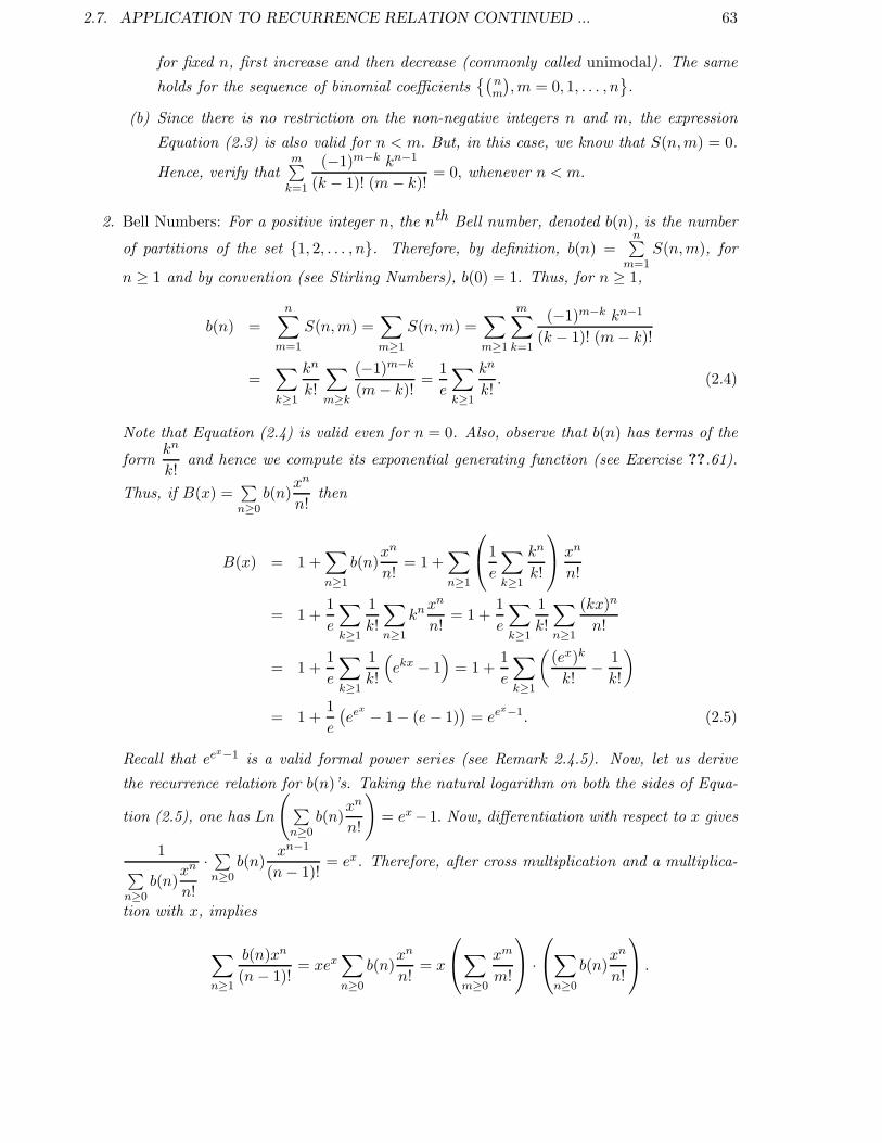
2.7. APPLICATION TO RECURRENCE RELATION CONTINUED ... 63
for fixed n, first increase and then decrease (commonly called unimodal). The same
holds for the sequence of binomial coefficients(
nm
),m = 0, 1, . . . , n
.
(b) Since there is no restriction on the non-negative integers n and m, the expression
Equation (2.3) is also valid for n < m. But, in this case, we know that S(n,m) = 0.
Hence, verify thatm∑
k=1
(−1)m−k kn−1
(k − 1)! (m− k)!= 0, whenever n < m.
2. Bell Numbers: For a positive integer n, the nth Bell number, denoted b(n), is the number
of partitions of the set 1, 2, . . . , n. Therefore, by definition, b(n) =n∑
m=1S(n,m), for
n ≥ 1 and by convention (see Stirling Numbers), b(0) = 1. Thus, for n ≥ 1,
b(n) =
n∑
m=1
S(n,m) =∑
m≥1
S(n,m) =∑
m≥1
m∑
k=1
(−1)m−k kn−1
(k − 1)! (m− k)!
=∑
k≥1
kn
k!
∑
m≥k
(−1)m−k
(m− k)!=
1
e
∑
k≥1
kn
k!. (2.4)
Note that Equation (2.4) is valid even for n = 0. Also, observe that b(n) has terms of the
formkn
k!and hence we compute its exponential generating function (see Exercise ??.61).
Thus, if B(x) =∑
n≥0b(n)
xn
n!then
B(x) = 1 +∑
n≥1
b(n)xn
n!= 1 +
∑
n≥1
1
e
∑
k≥1
kn
k!
xn
n!
= 1 +1
e
∑
k≥1
1
k!
∑
n≥1
knxn
n!= 1 +
1
e
∑
k≥1
1
k!
∑
n≥1
(kx)n
n!
= 1 +1
e
∑
k≥1
1
k!
(
ekx − 1)
= 1 +1
e
∑
k≥1
((ex)k
k!− 1
k!
)
= 1 +1
e
(ee
x − 1− (e− 1))= ee
x−1. (2.5)
Recall that eex−1 is a valid formal power series (see Remark 2.4.5). Now, let us derive
the recurrence relation for b(n)’s. Taking the natural logarithm on both the sides of Equa-
tion (2.5), one has Ln
(
∑
n≥0b(n)
xn
n!
)
= ex−1. Now, differentiation with respect to x gives
1∑
n≥0b(n)
xn
n!
· ∑n≥0
b(n)xn−1
(n− 1)!= ex. Therefore, after cross multiplication and a multiplica-
tion with x, implies
∑
n≥1
b(n)xn
(n− 1)!= xex
∑
n≥0
b(n)xn
n!= x
∑
m≥0
xm
m!
·
∑
n≥0
b(n)xn
n!
.
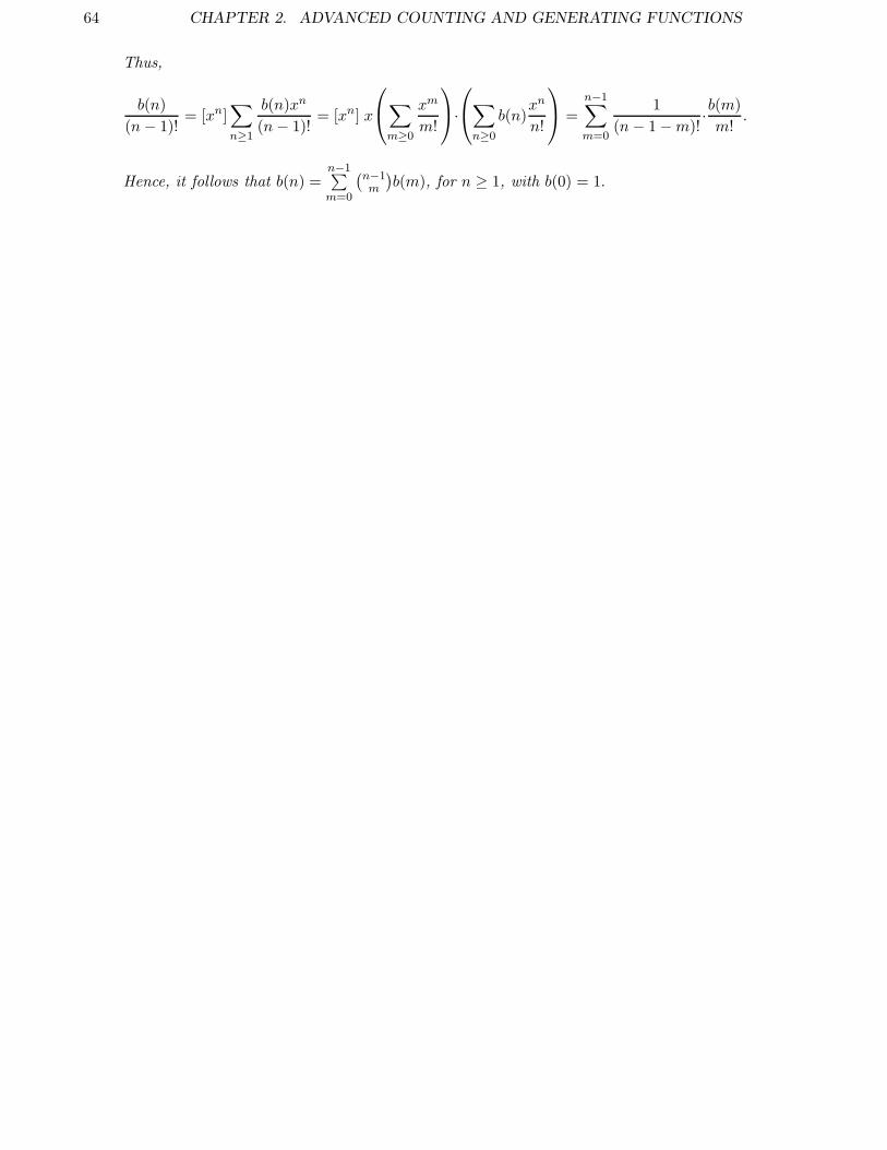
64 CHAPTER 2. ADVANCED COUNTING AND GENERATING FUNCTIONS
Thus,
b(n)
(n− 1)!= [xn]
∑
n≥1
b(n)xn
(n− 1)!= [xn] x
∑
m≥0
xm
m!
·
∑
n≥0
b(n)xn
n!
=
n−1∑
m=0
1
(n− 1−m)!·b(m)
m!.
Hence, it follows that b(n) =n−1∑
m=0
(n−1m
)b(m), for n ≥ 1, with b(0) = 1.

2.8. APPLICATION TO RECURRENCE RELATION CONTINUED ... 65
2.8 Application to Recurrence Relation Continued ...
Example 2.8.1. Determine the number of ways of arranging n pairs of parentheses (left and
right) such that at any stage the number of right parentheses is always less than or equal to the
number of left parentheses.
Solution: Recall that this number equals Cn, the nth Catalan number (see Page 39). Let us
obtain a recurrence relation for these numbers and use it to get a formula for Cn’s.
Let Pn denote the arrangements of those n pairs of parentheses that satisfy “at any stage, the
number of left parentheses is always greater than or equal to the number of right parentheses”.
Then |Pn| = Cn, for all n ≥ 1. Also, let Qn denote those elements of Pn for which, “at the
2k-th stage, for k < n, the number of left parentheses is strictly greater than the number of right
parentheses”.
We now claim that |Q1| = 1 and |Qn| = |Pn−1|, for n ≥ 2.
Clearly |Q1| = 1. Note that, for n ≥ 2, any element of Qn, necessarily starts with two left
parentheses and ends with two right parentheses. So, if we remove the first left parenthesis and
the last right parenthesis from each element of Qn then one obtains an element of Pn−1. In a
similar way, if we add one left parenthesis at the beginning and a right parenthesis at the end of
an element of Pn−1, one obtains an element of Qn. Hence, there is one-to-one correspondence
between the set Qn and Pn−1. Thus, |Qn| = |Pn−1| = Cn−1.
Let n ≥ 2 and consider an element of Pn. Then, for some k, 1 ≤ k ≤ n, the first k pairs of
parentheses will have the property that the number of left parentheses is strictly greater than the
number of right parentheses, for 1 ≤ ℓ < k, i.e., they form an element of Qk and the remaining
(n − k) pairs of parentheses will form an element of Pn−k. Hence, if |P0| = |Q1| = 1, one
has Cn = |Pn| =n∑
k=1
|Qk||Pn−k| =n∑
k=1
|Pk−1||Pn−k| =n∑
k=1
Ck−1Cn−k, for n ≥ 2. Now, define
C(x) =∑
n≥0Cnx
n. Then
C(x) =∑
n≥0
Cnxn = 1 +
∑
n≥1
Cnxn = 1 +
∑
n≥1
(n∑
k=1
Ck−1Cn−k
)
xn
= 1 + x
∑
k≥1
Ck−1xk−1
∑
n≥k
Cn−kxn−k
= 1 + x
C(x)∑
k≥1
Ck−1xk−1
= 1 + x (C(x))2 .
Thus, x C(x)2 − C(x) + 1 = 0 and C(x) =1±
√1− 4x
2x. Therefore, using C0 = 1, one obtains

66 CHAPTER 2. ADVANCED COUNTING AND GENERATING FUNCTIONS
C(x) =1−
√1− 4x
2x. Hence,
Cn = [xn]C(x) =1
2· [xn+1]
(1−
√1− 4x
)
= −1
2·
1
2
(1
2− 1
)(1
2− 2
)
· · ·(1
2− n
)
(n+ 1)!(−4)n+1
= 2(−4)n · 1 · (−1) · (−3) · (−5) · · · (1− 2n)
2n+1(n+ 1)!= 2n
1 · 3 · 5 · · · (2n − 1)
(n + 1)!
=1
n+ 1
(2n
n
)
, the nth Catalan Number.
The ideas learnt in the previous sections will be used to get closed form expressions for sums
arising out of binomial coefficients. To do so, recall the list of formal power series that appear
on Page 58.
Example 2.8.2. 1. Find a closed form expression for the numbers a(n) =∑
k≥0
( kn−k
).
Solution: Define A(x) =∑
n≥0a(n)xn. Then
A(x) =∑
n≥0
a(n)xn =∑
n≥0
∑
k≥0
(k
n− k
)
xn =∑
k≥0
∑
n≥0
(k
n− k
)
xn
=∑
k≥0
xk
∑
n≥k
(k
n− k
)
xn−k
=∑
k≥0
xk(1 + x)k =∑
k≥0
(x(1 + x)
)k=
1
1− x(1 + x).
Therefore, Example 2.6.1.2 implies a(n) = [xn]A(x) = [xn]1
1− x(1 + x)= Fn, the n-th
Fibonacci number.
2. Find a closed form expression for the polynomials a(n, x) =⌊n2⌋
∑
k=0
(n−kk
)(−1)kxn−2k.
Solution: Define A(x, y) =∑
n≥0a(n, x)yn. Then
A(x, y) =∑
n≥0
a(n, x)yn =∑
n≥0
⌊n2⌋
∑
k=0
(n− k
k
)
(−1)kxn−2k
yn
=∑
k≥0
(−1)ky2k
∑
n≥2k
(n− k
k
)
(xy)n−2k
=∑
k≥0
(−1)ky2k(xy)−k
∑
t≥k
(t
k
)
(xy)t
=∑
k≥0
(−y2)k(xy)−k (xy)k
(1− xy)k+1=
1
1− xy·∑
k≥0
( −y21− xy
)k
=1
1− xy· 1
1− −y2
1−xy
=1
1− xy + y2=
1
(1− αy)(1 − βy),

2.8. APPLICATION TO RECURRENCE RELATION CONTINUED ... 67
where α =x+
√x2 − 4
2and β =
x−√x2 − 4
2. Thus,
a(n, x) = [yn]A(x, y) = [yn]1
1− xy + y2= [yn]
1
α− β
(α
1− αy− β
1− βy
)
=1
α− β
(αn+1 − βn+1
)
=1√
x2 − 4
(
x+√x2 − 4
2
)n+1
−(
x−√x2 − 4
2
)n+1
.
Since α and β are the roots of y2 − xy + 1 = 0, α2 = αx− 1 and β2 = βx− 1. Therefore,
verify that the a(n, x)’s satisfy the recurrence relation a(n, x) = xa(n− 1, x)− a(n− 2, x),
for n ≥ 2, with initial conditions a(0, x) = 1 and a(1, x) = x.
Let A = (aij) be an n×n matrix, with aij = 1, whenever |i−j| = 1 and 0, otherwise. Then
A is an adjacency matrix of a tree T on n vertices, say 1, 2, . . . , n with the vertex i being
adjacent to i+ 1, for 1 ≤ i ≤ n − 1. It can be verified that if a(n, x) = det(xIn − A), the
characteristic polynomial of A, then a(n, x)’s satisfy the above recurrence relation. The
polynomials a(n, 2x)’s are also known as Chebyshev’s polynomial of second kind.

68 CHAPTER 2. ADVANCED COUNTING AND GENERATING FUNCTIONS
2.9 Applications to Generating Functions Continued ...
Let us now substitute different values for x to obtain different expressions and then use them to
get binomial identities.
1. Let x = z+1
z. Then
√x2 − 4 = z − 1
zand we obtain a(n, z + 1
z ) =z2n+2 − 1
(z2 − 1)zn. Hence, we
have⌊n2⌋
∑
k=0
(n−kk
)(−1)k
(z + 1
z
)n−2k=
z2n+2 − 1
(z2 − 1)zn. Or equivalently,
⌊n2⌋
∑
k=0
(n− k
k
)
(−1)k(z2 + 1
)n−2kz2k =
z2n+2 − 1
z2 − 1.
2. Writing x in place of z2, we obtain the following identity.
⌊n2⌋
∑
k=0
(n− k
k
)
(−1)k (x+ 1)n−2k xk =xn+1 − 1
x− 1=
n∑
k=0
xk. (2.1)
3. Hence, equating the coefficient of xm in (2.1) gives the identity
⌊n2⌋
∑
k=0
(−1)k(n− k
k
)(n− 2k
m− k
)
=
1, if 0 ≤ m ≤ n;
0, otherwise.
4. Substituting x = 1 in (2.1) gives⌊n2⌋
∑
k=0
(−1)k(n−k
k
)2n−2k = n+ 1.
Example 2.9.1. Determine the generating function for the numbers a(n, y) =∑
k≥0
(n+k2k
)yk.
Solution: Define A(x, y) =∑
n≥0a(n, y)xn. Then
A(x, y) =∑
n≥0
∑
k≥0
(n+ k
2k
)
yk
xn =∑
k≥0
(y
x
)k∑
n≥k
(n+ k
2k
)
xn+k
=∑
k≥0
(y
x
)k x2k
(1− x)2k+1=
1
1− x
∑
k≥0
(yx
(1− x)2
)k
=1− x
(1− x)2 − xy.
1. Verify that if we substituting y = −2 then
∑
k≥0
(n+ k
2k
)
(−2)k = [xn] A(x,−2) = [xn]1− x
(1 + x2)= (−1)⌈n/2⌉.
2. Verify that if we substituting y = −4 then
∑
k≥0
(n+ k
2k
)
(−4)k = [xn] A(x,−4) = [xn]1− x
(1 + x)2= (−1)n(2n+ 1).

2.9. APPLICATIONS TO GENERATING FUNCTIONS CONTINUED ... 69
3. Let f(n) =∑
k≥0
(n+k2k
)2n−k and let F (z) =
∑
n≥0f(n)zn. Then verify that
F (z) = A(2z,1
2) =
1− 2z
(1 − z)(1 − 4z)=
2
3· 1
1− 4z+
1
3· 1
1− z.
Hence, f(n) = [zn]F (z) =2 · 4n3
+1
3=
22n+1 + 1
3.
Notes: Most of the ideas for this chapter have come from book [11].
Chapter 3
Groups and Polya Theory
3.1 Groups
Our aim in this chapter is to look at groups and use it to the study of questions of the type:
1. How many different necklace configurations are possible if we use 6 beads of 3 different
colors? Or, for that matter what if we use n beads of m different colors?
2. How many different necklace configurations are possible if we use 12 beads among which
3 are red, 5 are blue and 4 are green? And a generalization of this problem.
3. Counting the number of chemical compounds which can be derived by the substitution of
a given set of radicals in a given molecular structure.
It can be easily observed that if we want to look at different color configurations of a necklace
formed using 6 beads, we need to understand the symmetries of a hexagon. Such a study is
achieved through what in literature is called groups. Once we have learnt a bit about groups,
we study group action. This study helps us in defining an equivalence relation on the set of
color configurations for a given necklace. And it turns out that the number of distinct color
configurations is same as the number of equivalence classes.
Before coming to the definition and its properties, let us look at the properties of the sets
N,Z,Q,R and C. We know that the sets Z,Q,R and C satisfy the following:
Binary Operation: for every a, b ∈ Z (Q,R,C), a + b, called the addition of a and b, is an
element of Z (Q,R,C);
Addition is Associative: for every a, b, c ∈ Z (Q,R,C), (a+ b) + c = a+ (b+ c);
Additive Identity: the element zero, denoted 0, is an element of Z (Q,R,C) and has the
property that for every a ∈ Z (Q,R,C), a+ 0 = a = 0+ a;
71

72 CHAPTER 3. GROUPS AND POLYA THEORY
Additive Inverse: For every element a ∈ Z (Q,R,C), there exists an element −a ∈ Z (Q,R,C)
such that a+ (−a) = 0 = −a+ a;
Addition is Commutative: We also have a+ b = b+ a for every a, b ∈ Z (Q,R,C).
Now, let us look at the sets Z∗ = Z− 0,Q∗ = Q− 0,R∗ = R − 0 and C∗ = C− 0.As in the previous case, we see that similar statements hold true for the sets Z∗,Q∗,R∗ and C∗.
Namely,
Binary Operation: for every a, b ∈ Z∗ (Q∗,R∗,C∗), a · b, called the multiplication of a and b,
is an element of Z∗ (Q∗,R∗,C∗);
Multiplication is Associative: for every a, b, c ∈ Z∗ (Q∗,R∗,C∗), (a · b) · c = a · (b · c);
Multiplicative Identity: the element one, denoted 1, is an element of Z∗ (Q∗,R∗,C∗) and for
all a ∈ Z∗ (Q∗,R∗,C∗), a · 1 = a = 1 · a;
Multiplication is Commutative: One also has a · b = b · a for every a, b ∈ Z∗ (Q∗,R∗,C∗).
Observe that if we choose a ∈ Z∗ with a 6= 1,−1 then there does not exist an element b ∈ Z∗
such that a · b = 1 = b ·a. Whereas, for the sets Q∗,R∗ and C∗ one can always find a b such that
a · b = 1 = b · a.Based on the above examples, an abstract notion called groups is defined. Formally, one
defines a group as follows.
Definition 3.1.1 (Group). A group G, usually denoted (G, ∗), is a non-empty set, together with
a binary operation, say ∗, such that the elements of G satisfy the following:
1. for every a, b, c ∈ G, (a ∗ b) ∗ c = a ∗ (b ∗ c) (Associativity Property) holds in G;
2. there is an element e ∈ G such that a∗e = a = e∗a, for all a ∈ G (Existence of Identity);
3. for every element a ∈ G, there exists an element b ∈ G such that a∗b = e = b∗a (Existence
of Inverse).
In addition, if the set G satisfies a∗b = b∗a, for every a, b ∈ G, then G is said to be an abelian
(commutative) group.
Before proceeding with examples of groups that concerns us, we state a few basic results in
group theory without proof. The readers are advised to prove it for themselves.
Remark 3.1.2. Let (G, ∗) be a group. Then the following hold:
1. The identity element of G is unique. Hence, the identity element is denoted by e.
2. For each fixed a ∈ G, the element b ∈ G such that a∗b = e = b∗a is also unique. Therefore,
for each a ∈ G, the element b that satisfies a ∗ b = e = b ∗ a is denoted by a−1.
3.1. GROUPS 73
3. Also, for each a ∈ G, (a−1)−1 = a.
4. If a∗b = a∗c, for some a, b, c ∈ G then b = c. Similarly, if b∗d = c∗d, for some b, c, d ∈ G
then b = c. That is, the cancelation laws in G.
5. For each a, b ∈ G, (ab)−1 = b−1a−1.
6. By convention, we assume a0 = e, for all a ∈ G.
7. For each a ∈ G, (an)−1 = (a−1)n, for all n ∈ Z.
In the remaining part of this chapter, the binary operation may not be explicitly mentioned
as it will be clear from the context. Now, let us now look at a few examples that will be used
later in this chapter.
Example 3.1.3. Symmetric group on n letters: Let N denote the set 1, 2, . . . , n. A
function f : N−→N is called a permutation on n elements if f is both one-to-one and onto. Let
Sn = f : N−→N | f is one to one and onto. That is, Sn is the set of all permutations of the
set 1, 2, . . . , n. Then the following can be verified:
1. Suppose f, g ∈ Sn. Then f : N−→N and g : N−→N are two one-to-one and onto func-
tions. Therefore, one uses the composition of functions to define the composite function
f g : N−→N by (f g)(x) = f(g(x)
). Then it can be easily verified that f g is also
one-to-one and onto. Hence f g ∈ Sn. That is, “composition of function”, denoted ,defines a binary operation in Sn.
2. It is well known that the composition of functions is an associative operation and thus
(f g) h = f (g h).
3. The function e : N−→N defined by e(i) = i, for all i = 1, 2, . . . , n is the identity function.
That is, check that f e = f = e f , for all f ∈ Sn.
4. Now let f ∈ Sn. As f : N−→N is a one-to-one and onto function, f−1 : N−→N defined
by f−1(i) = j, whenever f(j) = i, for all i = 1, 2, . . . , n, is a well defined function and is
also one-to-one and onto. That is, for each f ∈ Sn, f−1 ∈ Sn and f f−1 = e = f−1 f .
Thus (Sn, ) is a group. This group is called the Symmetric/Permutation group on n letters. If
σ ∈ Sn then one represents this by writing σ =
(
1 2 · · · n
σ(1) σ(2) · · · σ(n)
)
. This representation
of an element of Sn is called a two row notation. Observe that as σ is one-to-one and onto
function from N to N , it can be checked that N = σ(1), σ(2), . . . , σ(n). Hence, there are n
choices for σ(1), n − 1 choices for σ(2) (all elements of N except σ(1)) and so on. Thus, the
total number of elements in Sn is n! = n(n− 1) · · · 2 · 1.
74 CHAPTER 3. GROUPS AND POLYA THEORY
Before discussing other examples, let us try to understand the group Sn. As seen above,
any element σ ∈ Sn can be represented using a two-row notation. There is another notation for
permutations that is often very useful. This notation is called the cycle notation. Let us try to
understand this notation.
Definition 3.1.4. Let σ ∈ Sn and let S = i1, i2, . . . , ik ⊆ 1, 2, . . . , n be distinct. If σ
satisfies
σ(iℓ) = iℓ+1, for all ℓ = 1, 2, . . . , k − 1, σ(ik) = i1 and σ(r) = r for r 6∈ S
then σ is called a k-cycle and is denoted by σ = (i1, i2, . . . ik) or (i2, i3, . . . , ik, i1) and so on.
Example 3.1.5. 1. The permutation σ =
(
1 2 3 4 5
2 3 4 1 5
)
in cycle notation can be written
as (1234), (2341), (3412), or (4123) as σ(1) = 2, σ(2) = 3, σ(3) = 4, σ(4) = 1 and σ(5) = 5.
2. The permutation
(
1 2 3 4 5 6
2 3 1 4 6 5
)
in cycle notation equals (123)(65) as σ(1) = 2, σ(2) =
3, σ(3) = 1, σ(4) = 4, σ(5) = 6 and σ(6) = 5. That is, this element is formed with the
help of two cycles (123) and (56).
3. Consider two permutations σ = (143)(27) and τ = (1357)(246). Then, there composition,
denoted σ τ , is obtained as follows:
(σ τ)(1) = σ(τ(1)
)= σ(3) = 1, (σ τ)(2) = σ
(τ(2)
)= σ(4) = 3, (σ τ)(3) = σ
(τ(3)
)=
σ(5) = 5, (στ)(4) = σ(τ(4)
)= σ(6) = 6, (στ)(5) = 2, (στ)(6) = 7 and (στ)(7) = 4.
Hence
σ τ = (143)(27)(1357)(246) =
(
1 2 3 4 5 6 7
1 3 5 6 2 7 4
)
= (235)(467).
4. Similarly, verify that (1456)(152) = (16)(245).
Definition 3.1.6. Two cycles σ = (i1, i2, . . . , it) and τ = (j1, j2, . . . , js) are said to be disjoint
if
i1, i2, . . . , it ∩ j1, j2, . . . , js = ∅.
The proof of the following theorem can be obtained from any standard book on abstract
algebra.
Theorem 3.1.7. Let σ ∈ Sn. Then σ can be written as a product of disjoint cycles.
Remark 3.1.8. Observe that the representation of a permutation as a product of disjoint cycles,
none of which is the identity, is unique up to the order of the disjoint cycles. The representation
of an element σ ∈ Sn as product of disjoint cycles is called the cyclic decomposition of σ.

3.2. EXAMPLE OF GROUPS 75
3.2 Example of Groups
Example 3.2.1. 1. Symmetries of regular n-gons in plane.
(a) Suppose a unit square is placed at the coordinates (0, 0, 0), (1, 0, 0), (0, 1, 0) and (1, 1, 0).
Our aim is to move the square in space such that the position of the vertices may
change but they are still placed at the above mentioned coordinates. The question
arises, what are the possible ways in which this can be done? It can be easily verified
that the possible configurations are as follows (see Figure 3.1):
r
rf
41
2 3
18023
4 1
9034
1 2
27012
3 4
f
r14
3 2
18032
1 4
9021
4 3
27043
2 1
Figure 3.1: Symmetries of a square.
Let r denote the counter-clockwise rotation of the square by 90 and f denote the
flipping of the square along the vertical axis passing through the midpoint of opposite
horizontal edges (see Figure 3.1). Then note that the possible configurations corre-
spond to the set
G = e, r, r2, r3, f, rf, r2f, r3f with relations r4 = e = f2 and fr3 = rf. (3.1)
Using (3.1), observe that (rf)2 = (rf)(rf) = r(fr)f = r(r3f)f = r4f2 = e. Sim-
ilarly, it can be checked that (r2f)2 = (r3f)2 = e. That is, all the terms f, rf, r2f
and r3f are flips. The group G is generally denoted by D4 and is called the Dihe-
dral group or the symmetries of a square. This group can also be represented as
follows:
e, (1234), (13)(24), (1432), (14)(23), (24), (12)(34), (13).
Exercise: Relate the two representations of the group D4.
(b) In the same way, one can define the symmetries of an equilateral triangle (see Figure
3.2). This group is denoted by D3 and is represented as
D3 = e, r, r2, f, rf, r2f with relations r3 = e = f2 and fr2 = rf, (3.2)

76 CHAPTER 3. GROUPS AND POLYA THEORY
where r is a counter-clockwise rotation by 120 =2π
3and f is a flip. Using Figure 3.2,
one can check that the group D3 can also be represented by
D3 = e, (ABC), (ACB), (BC), (CA), (AB).
r
B
C
A
120
C
A
B
240
A
B
C
rff
r
A
C
B
120
C
B
A
240
B
A
C
Figure 3.2: Symmetries of an Equilateral Triangle.
(c) For a regular pentagon, it can be verified that the group of symmetries of a regular
pentagon is given by G = e, r, r2, r3, r4, f, rf, r2f, r3f, r4f with r5 = 2 = f2 and
rf = fr4, where r denotes a counter-clockwise rotation through an angle of 72 =2π
5and f is a flip along a line that passes through a vertex and the midpoint of the opposite
edge. Or equivalently, if we label the vertices of a regular pentagon, counter-clockwise,
with the numbers 1, 2, 3, 4 and 5 then
G = e, (1, 2, 3, 4, 5), (1, 3, 5, 2, 4), (1, 4, 2, 5, 3), (1, 5, 4, 3, 2), (2, 5)(3, 4),(1, 3)(4, 5), (1, 5)(2, 4), (1, 2)(3, 5), (1, 4)(2, 3).
(d) In general, one can define symmetries of a regular n-gon. This group is denoted by
Dn,has 2n elements and is represented as
e, r, r2, . . . , rn−1, f, rf, . . . , rn−1f with rn = e = f2 and frn−1 = rf. (3.3)
Here the symbol r stands for a counter-clockwise rotation through an angle of2π
nand
f stands for a vertical flip.
2. Symmetries of regular platonic solids.
(a) Recall from geometry that a tetrahedron is a 3-dimensional regular object that is com-
posed of 4-equilateral triangles such that any three triangles meet at a vertex (see

3.2. EXAMPLE OF GROUPS 77
Figure 3.1). Observe that a tetrahedron has 6 edges, 4 vertices and 4 faces. If we
denote the vertices of the tetrahedron with numbers 1, 2, 3 and 4, then the symmetries
of the tetrahedron can be represented with the help of the group,
G = e, (234), (243), (124), (142), (123), (132), (134), (143), (12)(34), (13)(24), (14)(23),
where, for distinct numbers i, j, k and ℓ, the element (ijk) is formed by a rotation of
120 along the line that passes through the vertex ℓ and the centroid of the equilateral
triangle with vertices i, j and k. Similarly, the group element (ij)(kℓ) is formed by
a rotation of 180 along the line that passes through mid-points of the edges (ij) and
(kℓ).
A DodecahedronAn Icosahedron
1
2
4
3
A Tetrahedron
12 3
4
56 7
8
A Cube
1
3
2
45
6
An Octahedron
Figure 3.3: Regular Platonic solids.
(b) Consider the Cube and the Octahedron given in Figure 3.3. It can be checked that the
group of symmetries of the two figures has 24 elements. We give the group elements
for the symmetries of the cube, when the vertices of the cube are labeled. The readers
are required to compute the group elements for the symmetries of the octahedron. For
the cube (see Figure 3.3), the group elements are
i. e, the identity element;
ii. 3 × 3 = 9 elements that are obtained by rotations along lines that pass through
the center of opposite faces (3 pairs of opposite faces and each face is a square:

78 CHAPTER 3. GROUPS AND POLYA THEORY
corresponds to a rotation of 90). In terms of the vertices of the cube, the group
elements are
(1234)(5678), (13)(24)(57)(68), (1432)(5876), (1265)(3784), (16)(25)(38)(47),
(1562)(3487), (1485)(2376), (18)(45)(27)(36), (1584)(2673).
iii. 2 × 4 = 8 elements that are obtained by rotations along lines that pass through
opposite vertices (4 pairs of opposite vertices and each vertex is incident with 3
edges: correspond to a rotation of 120). The group elements in terms of the
vertices of the cube are
(254)(368), (245)(386), (163)(457), (136)(475), (275)(138),
(257)(183), (168)(274), (186)(247).
iv. 1×6 = 6 elements that are obtained by rotations along lines that pass through the
midpoint of opposite edges (6 pairs of opposite edges: corresponds to a rotation
of 180). The corresponding elements in terms of the vertices of the cube are
(14)(67)(28)(35), (23)(58)(17)(46), (15)(37)(28)(64), (26)(48)(17)(35),
(12)(78)(35)(46), (34)(56)(17)(28).
12 3
4
56 7
8
90 rotations along lines that
pass through opposite faces.
12 3
4
56 7
8
120 rotations along lines that
pass through opposite vertices.
12 3
4
56 7
8
180 rotations along lines that
pass through opposite edges.
Figure 3.4: Understanding the group of symmetries of a cube.
(c) Consider now the icosahedron and the dodecahedron (see Figure 3.3). Note that the
icosahedron has 12 vertices, 20 faces and 30 edges and the dodecahedron has 20 ver-
tices, 12 faces and 30 edges. It can be checked that the group of symmetries of the two
figures has 60 elements. We give the idea of the group elements for the symmetries
of the icosahedron. The readers are required to compute the group elements for the
symmetries of the dodecahedron. For the icosahedron, one has
i. e, the identity element;
ii. 2× 10 = 20 elements that are obtained by rotations along lines that pass through
the center of opposite faces (10 pairs of opposite faces and each face is an equi-
lateral triangle: corresponds to a rotation of 120);

3.2. EXAMPLE OF GROUPS 79
iii. 6 × 4 = 24 elements that are obtained by rotations along lines that pass through
opposite vertices (6 pairs of opposite vertices and each vertex is incident with 5
edges: corresponds to a rotation of 72);
iv. 1× 15 = 15 elements that are obtained by rotations along lines that pass through
the midpoint of opposite edges (15 pairs of opposite edges: corresponds to a rota-
tion of 180).

80 CHAPTER 3. GROUPS AND POLYA THEORY
3.3 SubGroups
To proceed further, we study the notion of subgroup of a given group. That is, if (G, ∗) is a
group and H is a non-empty subset of G then under what condition is (H, ∗) a group in its own
right (it is important to note that the binary operation is the same as that in G). Formally, we
have the following definition.
Definition 3.3.1 (Subgroup). Let (G, ∗) be a group. Then a non-empty subset H of G is said
to be a subgroup of G, if H itself forms a group with respect to the binary operation ∗.
Example 3.3.2. 1. Let G be a group with identity element e. Then G and e are them-
selves groups and hence they are subgroups of G. These two subgroups are called trivial
subgroups.
2. Z, the set of integers, and Q, the set of rational numbers, are subgroups of (R,+), the set
of real numbers with respect to addition.
3. The set e, r2, f, r2f forms a subgroup of D4.
4. Let σ ∈ S4. Then, using Theorem 3.1.7, we know that σ has a cycle representation. With
this understanding it can be easily verified that the group D4 is a subgroup of S4.
5. Consider H = e, r, r2, . . . , rn−1 as a subset of Dn. Then it can be easily verified that H
is a subgroup of D4. This subgroup is also written as 〈r〉 to indicate that it is generated by
the element r of D4.
Before proceeding further, let us look at the following two results which help us in proving
“whether or not a given non-empty subset H of a group G is a subgroup of G”?
Theorem 3.3.3 (Subgroup Test). Let G be a group and let H be a non-empty subset of G.
Then H is a subgroup of G if for each a, b ∈ H, ab−1 ∈ H.
Proof. As H is non-empty, we can find an x ∈ H. Therefore, for a = x and b = x, the
condition ab−1 ∈ H implies that e = aa−1 ∈ H. Thus, H has the identity element of G. Hence,
for each h ∈ H ⊂ G, eh = h = he.
We now need to prove that for each h ∈ H, h−1 ∈ H. To do so, note that for a = e and
b = h the condition ab−1 ∈ H reduces to h−1 = eh−1 ∈ H.
As a third step, we show that H is closed with respect to the binary operation of G. So, let
us assume that x, y ∈ H. Then by the previous paragraph, y−1 ∈ H. Therefore, for a = x and
b = y−1 the condition ab−1 ∈ H implies that xy = x(y−1)−1 ∈ H. Hence, H is also closed with
respect to the binary operation of G.
Finally, we see that since the binary operation ofH is same as that ofG and since associativity
holds in G, it holds in H as well.

3.3. SUBGROUPS 81
We now give another result without proof that helps us in deciding whether a non-empty
subset of a group is a subgroup or not.
Theorem 3.3.4. [Two-Step Subgroup Test] Let H be a non-empty subset of a group G. Then
H is a subgroup if the two conditions given below hold.
1. For each a, b ∈ H, ab ∈ H (i.e., H is closed with respect to the binary operation of G).
2. For each a ∈ H, a−1 ∈ H.
We now give a few examples to understand the above theorems.
Example 3.3.5. 1. Consider the group (Z,+). Then in the following cases, the given subsets
do not form a subgroup.
(a) Let H = 0, 1, 2, 3, . . . ⊂ Z. Note that, for each a, b ∈ H, a+ b ∈ H and the identity
element 0 ∈ H. But H is not a subgroup of Z, as for all n 6= 0, −n 6∈ H.
(b) Let H = Z \ 0 = . . . ,−3,−2,−1, 1, 2, 3, . . . ⊂ Z. Note that, the identity element
0 6∈ H and hence H is not a subgroup of Z.
(c) Let H = −1, 0, 1 ⊂ Z. Then H contains the identity element 0 of Z and for each
h ∈ H, h−1 = −h ∈ H. But H is not a subgroup of Z as 1 + 1 = 2 6∈ H.
2. Let G be an abelian group with identity e. Consider the sets H = x ∈ G : x2 = e and
K = x2 : x ∈ G. Then prove that both H and K are subgroups of G.
Proof. Clearly e ∈ H and e ∈ K. Hence, both H and K are non-empty subsets of G. We
first show that H is a subgroup of G.
As H is non-empty, pick x, y ∈ H. Thus, x2 = e = y2. We will now use Theorem 3.3.3,
to show that xy−1 ∈ H. But this is equivalent to showing that(xy−1
)2= e. But this is
clearly true as G is abelian implies that
(xy−1
)2= x2(y−1)2 = e(y2)−1 = e−1 = e.
Thus, H is indeed a subgroup of G by Theorem 3.3.3.
Now, let us prove that K is a subgroup of G. We have already seen that K is non-empty.
Thus, we just need to show that for each x, y ∈ K, xy−1 ∈ K.
Note that x, y ∈ K implies that there exists a, b ∈ G such that x = a2 and y = b2. As
b ∈ G, b−1 ∈ G. Also, xy−1 = a2(b2)−1 = a2(b−1)2 = (ab−1)2 ∈ K as G is abelian and
ab−1 ∈ G. Thus, K is also a subgroup of G.
As a last result of this section, we prove that the condition of the above theorems can be
weakened if we assume that H is a finite, non-empty subset of a group G.
82 CHAPTER 3. GROUPS AND POLYA THEORY
Theorem 3.3.6. [Finite Subgroup Test] Let G be a group and let H be a non-empty finite subset
of G. If H is closed with respect to the binary operation of G then H is a subgroup of G.
Proof. By Theorem 3.3.4, we just need to show that for each a ∈ H, a−1 ∈ H. If
a = e ∈ H then a−1 = e−1 = e ∈ H. So, let us assume that a 6= e and a ∈ H. Now consider
the set S = a, a2, a3, . . . , an, . . .. As H is closed with respect to the binary operation of G,
S ⊂ H. But H has only finite number of elements. Hence, all these elements of S cannot be
distinct. That is, there exist positive integers, say m,n with m > n, such that am = an. Thus,
using Remark 3.1.2, one has am−n = e. Hence, a−1 = am−n−1 and by definition am−n−1 ∈ H.
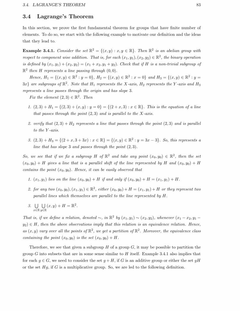
3.4. LAGRANGE’S THEOREM 83
3.4 Lagrange’s Theorem
In this section, we prove the first fundamental theorem for groups that have finite number of
elements. To do so, we start with the following example to motivate our definition and the ideas
that they lead to.
Example 3.4.1. Consider the set R2 = (x, y) : x, y ∈ R. Then R2 is an abelian group with
respect to component wise addition. That is, for each (x1, y1), (x2, y2) ∈ R2, the binary operation
is defined by (x1, y1) + (x2, y2) = (x1 + x2, y1 + y2). Check that if H is a non-trivial subgroup of
R2 then H represents a line passing through (0, 0).
Hence, H1 = (x, y) ∈ R2 : y = 0, H2 = (x, y) ∈ R2 : x = 0 and H3 = (x, y) ∈ R2 : y =
3x are subgroups of R2. Note that H1 represents the X-axis, H2 represents the Y -axis and H3
represents a line passes through the origin and has slope 3.
Fix the element (2, 3) ∈ R2. Then
1. (2, 3) +H1 = (2, 3) + (x, y) : y = 0 = (2 + x, 3) : x ∈ R. This is the equation of a line
that passes through the point (2, 3) and is parallel to the X-axis.
2. verify that (2, 3) +H2 represents a line that passes through the point (2, 3) and is parallel
to the Y -axis.
3. (2, 3) +H3 = (2 + x, 3 + 3x) : x ∈ R = (x, y) ∈ R2 : y = 3x − 3. So, this represents a
line that has slope 3 and passes through the point (2, 3).
So, we see that if we fix a subgroup H of R2 and take any point (x0, y0) ∈ R2, then the set
(x0, y0) + H gives a line that is a parallel shift of the line represented by H and (x0, y0) + H
contains the point (x0, y0). Hence, it can be easily observed that
1. (x1, y1) lies on the line (x0, y0) +H if and only if (x0, y0) +H = (x1, y1) +H.
2. for any two (x0, y0), (x1, y1) ∈ R2, either (x0, y0)+H = (x1, y1)+H or they represent two
parallel lines which themselves are parallel to the line represented by H.
3.⋃
x∈R
⋃
y∈R
(x, y) +H = R2.
That is, if we define a relation, denoted ∼, in R2 by (x1, y1) ∼ (x2, y2), whenever (x1 − x2, y1 −y2) ∈ H, then the above observations imply that this relation is an equivalence relation. Hence,
as (x, y) vary over all the points of R2, we get a partition of R2. Moreover, the equivalence class
containing the point (x0, y0) is the set (x0, y0) +H.
Therefore, we see that given a subgroup H of a group G, it may be possible to partition the
group G into subsets that are in some sense similar to H itself. Example 3.4.1 also implies that
for each g ∈ G, we need to consider the set g+H, if G is an additive group or either the set gH
or the set Hg, if G is a multiplicative group. So, we are led to the following definition.

84 CHAPTER 3. GROUPS AND POLYA THEORY
Definition 3.4.2 (Left and Right Coset). Let G be a group and let H be a subgroup of G. Then
for each g ∈ G the set
1. gH = gh : h ∈ H is called the left coset of H in G.
2. Hg = hg : h ∈ H is called the right coset of H in G.
Remark 3.4.3. Since the identity element e ∈ H, for each fixed g ∈ G, g = ge ∈ gH. Hence,
we often say that gH is the left coset of H containing g. Similarly, g ∈ Hg and hence Hg is
said to be the right coset of H containing g.
Example 3.4.4. Consider the group D4 and let H = e, f and K = e, r2 be two subgroups
of D4. Then observe the following:
H = e, f = Hf, Hr = r, fr = H fr,
H r2 = r2, fr2 = H fr2 and H r3 = r3, fr3 = H fr3. (3.1)
H = e, f = fH, rH = r, rf = rf H,
r2 H = r2, r2f = r2f H and r3 H = r3, r3f = r3f H. (3.2)
K = e, r2 = Kr2 = r2K, Kr = r, r3 = rK = Kr3 = r3K
Kf = f, r2f = fK = K r2f = r2f K and
K fr = fr, fr3 = fr K = K fr3 = fr3 K. (3.3)
From (3.1) and (3.2), we note that in general Hg 6= gH, for each g ∈ D4, whereas from (3.3),
we see that Kg = gK, for each g ∈ D4. So, there should be a way to distinguish between these
two subgroups of D4. This leads to study of normal subgroups and beyond. The interested reader
can look at any standard book in abstract algebra to go further in this direction.
Now, let us come back to the partition of a group using its subgroup. The proof of the
theorem is left as an exercise for the readers.
Theorem 3.4.5. Let H be a subgroup of a group G. Suppose a, b ∈ G. Then the following
results hold for left cosets of H in G:
1. aH = H if and only if a ∈ H,
2. aH is a subgroup of G if and only if a ∈ H,
3. either aH = bH or aH ∩ bH = ∅,
4. aH = bH if and only if a−1b ∈ H.
Similarly one obtains the following results for right cosets of H in G.
1. Ha = H if and only if a ∈ H,

3.4. LAGRANGE’S THEOREM 85
2. Ha is a subgroup of G if and only if a ∈ H,
3. either Ha = Hb or Ha ∩Hb = ∅,
4. Ha = Hb if and only if ab−1 ∈ H.
Furthermore, aH = Ha if and only if H = aHa−1 = aha−1 : h ∈ H.
To proceed further, we need the following definition.
Definition 3.4.6 (Order of a Group). The number of elements in G, denoted |G|, is called the
order of G. If |G| <∞, then G is called a group of finite order.
We are now ready to prove the main result of this section, namely the Lagrange’s Theorem.
Theorem 3.4.7. Let H be a subgroup of a finite group G. Then |H| divides |G|. Moreover, the
number of distinct left (right) cosets of H in G equals|G||H| .
Proof. We give the proof for left cosets. A similar proof holds for right cosets. Since G
is a finite group, the number of left cosets of H in G is finite. Let g1H, g2H, . . . , gmH be the
collection of all left cosets of H in G. Then by Theorem 3.4.5, two cosets are either equal or
they are disjoint. That is, G is a disjoint union of the sets g1H, g2H, . . . , gmH.
Also, it can be easily verified that |aH| = |bH|, for each a, b ∈ G. Hence, |giH| = |H|, for alli = 1, 2, . . . ,m. Thus, |G| =
∣∣∣∣
m⋃
i=1giH
∣∣∣∣=
m∑
i=1|giH| = m|H| (the disjoint union gives the second
equality). Thus, |H| divides |G| and the number of left cosets equals m =|G||H| .
Remark 3.4.8. The number m in Theorem 3.4.7 is called the index of H in G, and is denoted
by [G : H] or iG(H).
Theorem 3.4.7 is a statement about any subgroup of a finite group. It may so happen that the
group G and its subgroup H may have infinite number of elements but the number of left (right)
cosets of H in G may be finite. One still talks of index of H in G in such cases. For example,
consider H = 10Z as a subgroup of the additive group Z. Then [Z : H] = 10. In general, for a
fixed positive integer m, consider the subgroup mZ of the additive group Z. Then it can be easily
verified that [Z : mZ] = m.

86 CHAPTER 3. GROUPS AND POLYA THEORY
3.5 Applications of Lagrange’s Theorem
Before coming to our next remark, we need the following definition and example.
Definition 3.5.1 (Order of an Element). Let G be a group and let g ∈ G. Then the smallest
positive integer m such that gm = e is called the order of g. If there is no such positive
integer then g is said to have infinite order. The order of an element is denoted by O(g).
Example 3.5.2. 1. The only element of order 1 in a group G is the identity element of G.
2. In D4, the elements r2, f, rf, r2f, r3f have order 2, whereas the elements r and r3 have
order 4.
With the definition of the order of an element, we now prove that in general, the converse of
Lagrange’s Theorem is not true. To see this consider the group G discussed in Example 3.2.1.2a.
This group has 12 elements and 6 divides 12. Whereas it can be shown that G doesn’t have a
subgroup of order 6. We give a proof for better understanding of cosets.
Proof. Let if possible, H be a subgroup of order 6 in G, where
G = e, (234), (243), (124), (142), (123), (132), (134), (143), (12)(34), (13)(24), (14)(23).
Observe that G has exactly 8 elements of the form (ijk), for distinct numbers i, j and k, and
each has order 3. Hence, G has exactly 8 elements of order 3. Let a ∈ G with O(a) = 3. Then
using Theorem 3.4.5, we see that cosets of H in G will be exactly 2 and at the same time, the
possible cosets could be H, aH and a2H (as a3 = e, no other coset exists). Hence, at most two
of the cosets H, aH and a2H are distinct. But, using Theorem 3.4.5, it can be easily verified
that the equality of any two of them gives a ∈ H. Therefore, all the 8 elements of order 3 must
be elements of H. That is, H must have at least 9 elements (8 elements of order 3 and one
identity). This is absurd as |H| = 6.
We now derive some important corollaries of Lagrange’s Theorem. We omit the proof as it
can be found in any standard textbook in abstract algebra. The first corollary is about the order
of an element of a finite group. The observation that for each g ∈ G, the set H = e, g, g2 , g3, . . .forms a subgroup of any finite group G gives the proof of the next result.
Corollary 3.5.3. Let G be a finite group and let g ∈ G. Then O(g) divides |G|.
Remark 3.5.4. Corollary 3.5.3 implies that if G is a finite group of order n then the possible
orders of its elements are the divisors of n. For example, if |G| = 30 then for each g ∈ G, O(g) ∈1, 2, 3, 5, 6, 10, 15, 30.
Let G be a finite group. Then in the first corollary, we have shown that for any g ∈ G, O(g)
divides |G|. Therefore, |G| = m ·O(g), for some positive integer m. Hence
g|G| = gm·O(g) = (gO(g))m = em = e.
This observation gives our next result.

3.5. APPLICATIONS OF LAGRANGE’S THEOREM 87
Corollary 3.5.5. Let G be a finite group. Then, for each g ∈ G, g|G| = e.
Let P be an odd prime and consider the set Z∗p = 1, 2, . . . , p − 1. Then, check that Z∗
p
forms a group with respect to the binary operation
a⊙ b = the remainder, when ab is divided by p.
Applying Corollary 3.5.5 to Z∗p gives the famous result called the Fermat’s Little Theorem. To
state this, recall that for a, b ∈ Z, the notation “a ≡ b (mod p)” indicates that p divides a− b.
Corollary 3.5.6. Let a be any positive integer and let p be a prime. Then ap−1 ≡ 1 (mod p),
if p does not divide a. In general, ap ≡ a (mod p).
We now state without proof a generalization of the Fermat’s Little Theorem, popularly
known as the Euler’s Theorem. to do so, let Un = k : 1 ≤ k ≤ n, gcd(k, n) = 1, for each
positive integer n. Then Un, with binary operation
a⊙ b = the remainder, when ab is divided by n
forms a group. Also, recall that the symbol ϕ(n) gives the number of integers between 1 and
n that are coprime to n. That is, |Un| = ϕ(n), for each positive integer n. Now applying
Corollary 3.5.5 to Un, gives the next result.
Corollary 3.5.7. Let a, n ∈ Z with n > 0. If gcd(a, n) = 1 then aϕ(n) ≡ 1 (mod n).
Example 3.5.8. 1. Find the unit place in the expansion of 131001.
Solution : Observe that 13 ≡ 3 (mod 10). So, 131001 ≡ 31001 (mod 10). Also, 3 ∈ U10
and therefore by Corollary 3.5.5, 3|U10| = 1 (mod 10). But |U10| = 4 and 1001 = 4·250+1.
Thus,
131001 ≡ 31001 ≡ 34·250+1 ≡ (34)250 · 31 ≡ 1 · 3 ≡ 3 (mod 10).
Hence, the unit place in the expansion of 131001 is 3.
2. Find the unit and tens place in the expansion of 231002.
Solution : Observe that 23 ∈ U100 and 23|U100| = 1 (mod 100). But |U100| = 40 and
1002 = 40 · 25 + 2. Hence
231002 ≡ 2340·25+2 ≡ (2340)25 · 232 ≡ 1 · 232 ≡ 529 ≡ 29 (mod 100).
Hence, the unit place is 9 and the tens place is 2 in the expansion of 231002.

88 CHAPTER 3. GROUPS AND POLYA THEORY
3.6 Group Action
Definition 3.6.1. Let (G, ·) be a group with identity e. Then G is said to act on a set X, if
there exists an operator ⋆ : G×X−→X satisfying the following conditions:
1. e ⋆ x = x, for all x ∈ X, and
2. g ⋆ (h ⋆ x) = (g · h) ⋆ x, for all x ∈ X and g, h ∈ G.
Remark 3.6.2. 1. Let us assume that X consists of a set of points and let us suppose that
the group G acts on X by moving the points. Then, Definition 3.6.1 can be interpreted as
follows:
(a) the first condition implies that the identity element of the group does not move any
element of X. That is, the points in X remain fixed when they are acted upon by the
identity element of G.
(b) the second condition implies that if a point, say x0 ∈ X, is first acted upon by an
element h ∈ G and then by an element g ∈ G then the final position of x0 is same as
the position it would have reached if it was acted exactly once by the element g ·h ∈ G.
2. Fix an element g ∈ G. Then the set g ⋆ x : x ∈ X = X.
For, otherwise, there exist x, y ∈ X such that g ⋆ x = g ⋆ y. Then, by definition,
x = e ⋆ x = (g−1 · g) ⋆ x = g−1 ⋆ (g ⋆ x) = g−1 ⋆ (g ⋆ y) = (g−1 · g) ⋆ y = e ⋆ y = y.
That is, g just permutes the elements of X. Or equivalently, each g ∈ G gives rise to a
one-one, onto function from X into itself.
3. There may exist g, h ∈ G, with g 6= h such that g ⋆ x = h ⋆ x, for all x ∈ X,.
Before proceeding further with definitions and results related with group action, let us look
at a few examples.
Example 3.6.3. 1. Consider the dihedral group D6 = e, r, . . . , r5, f, rf, . . . , r5f, with r6 =e = f2 and rf = fr5. Here, f stands for the vertical flip and r stands for counter clockwise
rotation by an angle ofπ
3. Then D6 acts on the labeled edges/vertices of a regular hexagon
by permuting the labeling of the edges/vertices (see Figure 3.5).
a1
a2a3
a4a5
a6
f−→
a3
a2a1
a6a5
a4
and 14
23
65
r2−→ 52
61
43
Figure 3.5: Action of f on labeled edges and of r2 on labeled vertices of a regular hexagon.
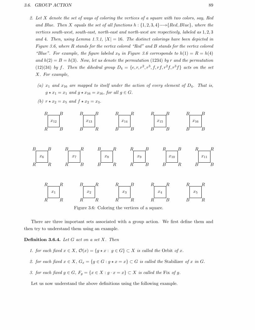
3.6. GROUP ACTION 89
2. Let X denote the set of ways of coloring the vertices of a square with two colors, say, Red
and Blue. Then X equals the set of all functions h : 1, 2, 3, 4−→Red,Blue, where the
vertices south-west, south-east, north-east and north-west are respectively, labeled as 1, 2, 3
and 4. Then, using Lemma 1.7.1, |X| = 16. The distinct colorings have been depicted in
Figure 3.6, where R stands for the vertex colored “Red” and B stands for the vertex colored
“Blue”. For example, the figure labeled x9 in Figure 3.6 corresponds to h(1) = R = h(4)
and h(2) = B = h(3). Now, let us denote the permutation (1234) by r and the permutation
(12)(34) by f . Then the dihedral group D4 = e, r, r2, r3, f, rf, r2f, r3f acts on the set
X. For example,
(a) x1 and x16 are mapped to itself under the action of every element of D4. That is,
g ⋆ x1 = x1 and g ⋆ x16 = x16, for all g ∈ G.
(b) r ⋆ x2 = x5 and f ⋆ x2 = x3.
x1
R
R R
R
x2
R
B R
R
x3
R
R B
R
x4
R
R R
B
x5
B
R R
R
x12
R
B B
B
x13
B
B B
R
x14
B
B R
B
x15
B
R B
B
x16
B
B B
B
x6
R
B B
R
x7
R
B R
B
x8
B
B R
R
x9
R
R B
B
x10
B
R B
R
x11
B
R R
B
Figure 3.6: Coloring the vertices of a square.
There are three important sets associated with a group action. We first define them and
then try to understand them using an example.
Definition 3.6.4. Let G act on a set X. Then
1. for each fixed x ∈ X, O(x) = g ⋆ x : g ∈ G ⊂ X is called the Orbit of x.
2. for each fixed x ∈ X, Gx = g ∈ G : g ⋆ x = x ⊂ G is called the Stabilizer of x in G.
3. for each fixed g ∈ G, Fg = x ∈ X : g · x = x ⊂ X is called the Fix of g.
Let us now understand the above definitions using the following example.

90 CHAPTER 3. GROUPS AND POLYA THEORY
Example 3.6.5. Consider the set X given in Example 3.6.3.2. Then using the depiction of the
set X in Figure 3.6, we have
O(x2) = x2, x3, x4, x5, Gx2 = e, rf, and Frf = x1, x2, x4, x7, x10, x13, x15, x16.
The readers should compute the different sets by taking other examples to understand the above
defined sets.
We now state a few results associated with the above definitions. The proofs are omitted as
they can be easily verified.
Proposition 3.6.6. Let G act on a set X.
1. Then for each fixed x ∈ X, the set Gx is a subgroup of G.
2. Define a relation, denoted ∼, on the set X, by x ∼ y if there exists g ∈ G, such that
g ⋆ x = y. Then prove that ∼ defines an equivalence relation on the set X. Furthermore,
the equivalence class containing x ∈ X equals O(x) = g ⋆ x : g ∈ G ⊂ X.
3. Fix x ∈ X and let t ∈ O(x). Then O(x) = O(t). Moreover, if g ⋆x = t then Gx = g−1Gtg.
Let G act on a set X. Then Proposition 3.6.6 helps us to relate the distinct orbits of X
under the action of G with the cosets of G. This is stated and proved as the next result.
Theorem 3.6.7. Let a group G act on a set X. Then for each fixed x ∈ X, there is a one-to-
one correspondence between the elements of O(x) and the set of all left cosets of Gx in G. In
particular,
|O(x)| = [G : Gx] = the number of left cosets of Gx in G.
Moreover, if G is a finite group then |G| = |O(x)| · |Gx|, for all x ∈ X.
Proof. Let S be the set of distinct left cosets of Gx in G. Then S = gGx : g ∈ G and
|S| = [G : Gx]. Consider the map τ : S−→O(x) by τ(gGx) = g ⋆ x. Let us first check that this
map is well-defined.
So, suppose that the left cosets gGx and hGx are equal. That is, gGx = hGx. Then,
using Theorem 3.4.5 and the definition of group action, one obtains the following sequence of
assertions:
gGx = hGx ⇐⇒ h−1g ∈ Gx ⇐⇒ (h−1g) ⋆ x = x⇐⇒ h−1 ⋆ (g ⋆ x) = x⇐⇒ g ⋆ x = h ⋆ x.
Thus, by definition of the map τ , one has gGx = hGx ⇐⇒ τ(gGx) = τ(hGx). Hence, τ is not
only well-defined but also one-one.
To show τ is onto, note that for each y ∈ O(x), there exists an h ∈ G, such that h ⋆ x = y.
Also, for this choice of h ∈ G, the coset hGx ∈ S. Therefore, for this choice of h ∈ G,
τ(hGx) = h ⋆ x = y holds. Hence, τ is onto.
3.6. GROUP ACTION 91
Therefore, we have shown that τ gives a one-to-one correspondence between O(x) and the
set S. This completes the proof of the first part. The other part follows by observing that by
definition ; [G : Gx] =|G||Gx|
, for each subgroup Gx of G whenever |G| is finite.The following lemmas are immediate consequences of Proposition 3.6.6 and Theorem 3.6.7.
We give the proof for the sake of completeness.
Lemma 3.6.8. Let G be a finite group acting on a set X. Then, for each y ∈ X,
∑
x∈O(y)
|Gx| = |G|.
Proof. Recall that, for each x ∈ O(y), |O(x)| = |O(y)|. Hence, using Theorem 3.6.7, one
has |G| = |Gx| · |O(x)|, for all x ∈ X. Therefore,
∑
x∈O(y)
|Gx| =∑
x∈O(y)
|G||O(x)| =
∑
x∈O(y)
|G||O(y)| =
|G||O(y)|
∑
x∈O(y)
1 =|G|
|O(y)| |O(y)| = |G|.
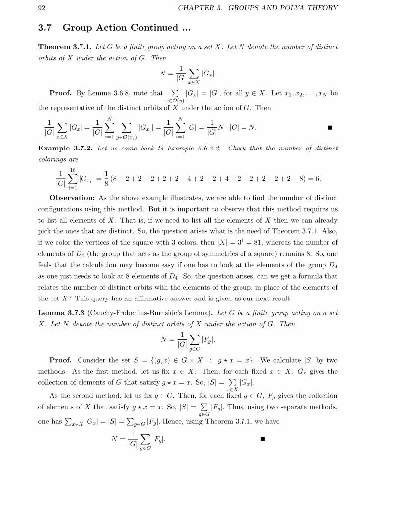
92 CHAPTER 3. GROUPS AND POLYA THEORY
3.7 Group Action Continued ...
Theorem 3.7.1. Let G be a finite group acting on a set X. Let N denote the number of distinct
orbits of X under the action of G. Then
N =1
|G|∑
x∈X
|Gx|.
Proof. By Lemma 3.6.8, note that∑
x∈O(y)
|Gx| = |G|, for all y ∈ X. Let x1, x2, . . . , xN be
the representative of the distinct orbits of X under the action of G. Then
1
|G|∑
x∈X
|Gx| =1
|G|N∑
i=1
∑
y∈O(xi)
|Gxi | =1
|G|N∑
i=1
|G| = 1
|G|N · |G| = N.
Example 3.7.2. Let us come back to Example 3.6.3.2. Check that the number of distinct
colorings are
1
|G|16∑
i=1
|Gxi | =1
8(8 + 2 + 2 + 2 + 2 + 2 + 4 + 2 + 2 + 4 + 2 + 2 + 2 + 2 + 2 + 8) = 6.
Observation: As the above example illustrates, we are able to find the number of distinct
configurations using this method. But it is important to observe that this method requires us
to list all elements of X. That is, if we need to list all the elements of X then we can already
pick the ones that are distinct. So, the question arises what is the need of Theorem 3.7.1. Also,
if we color the vertices of the square with 3 colors, then |X| = 34 = 81, whereas the number of
elements of D4 (the group that acts as the group of symmetries of a square) remains 8. So, one
feels that the calculation may become easy if one has to look at the elements of the group D4
as one just needs to look at 8 elements of D4. So, the question arises, can we get a formula that
relates the number of distinct orbits with the elements of the group, in place of the elements of
the set X? This query has an affirmative answer and is given as our next result.
Lemma 3.7.3 (Cauchy-Frobenius-Burnside’s Lemma). Let G be a finite group acting on a set
X. Let N denote the number of distinct orbits of X under the action of G. Then
N =1
|G|∑
g∈G
|Fg|.
Proof. Consider the set S = (g, x) ∈ G × X : g ⋆ x = x. We calculate |S| by two
methods. As the first method, let us fix x ∈ X. Then, for each fixed x ∈ X, Gx gives the
collection of elements of G that satisfy g ⋆ x = x. So, |S| = ∑
x∈X|Gx|.
As the second method, let us fix g ∈ G. Then, for each fixed g ∈ G, Fg gives the collection
of elements of X that satisfy g ⋆ x = x. So, |S| = ∑
g∈G|Fg|. Thus, using two separate methods,
one has∑
x∈X |Gx| = |S| =∑g∈G |Fg|. Hence, using Theorem 3.7.1, we have
N =1
|G|∑
g∈G
|Fg|.
3.7. GROUP ACTION CONTINUED ... 93
Example 3.7.4. Let us come back to Example 3.6.3.2. Check that |Fe| = 16, |Fr| = 2, |Fr2 | =4, |Fr3 | = 2, |Ff | = 4, |Frf | = 8, |Fr2f | = 4 and |Fr3f | = 8. Hence, the number of distinct
configurations are
1
|G|∑
g∈G
|Fg| =1
8(16 + 2 + 4 + 2 + 4 + 8 + 4 + 8) = 6.
It seems that we may still need to know all the elements of X to compute the above terms.
But it will be shown in the next section that to compute |Fg|, for any g ∈ G, we just need to
know the decomposition of g as product of disjoint cycles.

94 CHAPTER 3. GROUPS AND POLYA THEORY
3.8 The Cycle Index Polynomial
Let G be a group acting on a set X. Then as mentioned at the end of the previous section,
we need to understand the cycle decomposition of each g ∈ G as product of disjoint cycles.
Redfield and Polya observed that elements of G with the same cyclic decomposition made the
same contribution to the sets of fixed points. They defined the notion of cycle index polynomial
to keep track of the cycle decomposition of the elements of G. Let us start with a few definitions
and examples to better understand the use of cycle decomposition of an element of a permutation
group.
Definition 3.8.1. A permutation σ ∈ Sn is said to have the cycle structure 1ℓ1 2ℓ2 · · ·nℓn, ifthe cycle representation of σ has ℓi cycles of length i, for 1 ≤ i ≤ n. Observe that
t∑
i=1i · ℓi = n.
Example 3.8.2. 1. Let e be the identity element of Sn. Then e = (1) (2) · · · (n) and hence
the cycle structure of e, as an element of Sn equals 1n.
2. Let σ =
(
1 2 3 4 5 6 7 8 9 10 11 12 13 14 15
3 6 7 10 14 1 2 13 15 4 11 5 8 12 9
)
. Then it can be
easily verified that in the cycle notation, σ = (1 3 7 2 6) (4 10) (5 14 12) (8 13) (9 15) (11).
Thus, the cycle structure of σ is 11233151.
3. Consider the group G of symmetries of the tetrahedron (see Example 3.2.1.2a). Then the
elements of G have the following cycle structure:
14 for exactly 1 element corresponding to the identity element;
1131 for exactly 8 elements corresponding to 3 cycles;
22 for exactly 3 elements corresponding to (12)(34), (13)(24)&(14)(23).
Definition 3.8.3. Let G be a permutation group on n symbols. For a fixed g ∈ G, let ℓk(g)
denote the number of cycles of length k, 1 ≤ k ≤ n, in the cycle representation of g. Then the
cycle index polynomial of G, as a permutation group on n symbols, is a polynomial in n variables
z1, z2, . . . , zn given by
PG(z1, z2, . . . , zn) =1
|G|
∑
g∈G
zℓ1(g)1 z
ℓ2(g)2 · · · zℓn(g)n
.
Before, we look at a few examples, note that for each fixed g ∈ G, the condition that g has
exactly ℓk(g) cycles of length k, 1 ≤ k ≤ n, implies that each term zℓ1(g)1 z
ℓ2(g)2 · · · zℓn(g)n in the
summation satisfies 1 · ℓ1(g) + 2 · ℓ2(g) + · · ·+ n · ℓn(g) = n.
Example 3.8.4. 1. Let G be the dihedral group D4 (see Example 3.2.1.2). Then
e = (1)(2)(3)(4)−→z41 , r = (1234)−→z4, r3 = (1432)−→z4, r
2 = (13)(24)−→z22 ,
f = (14)(23)−→z22 , rf = (1)(3)(24)−→z21z2, r2f = (12)(34)−→z22 , r
3f = (13)(2)(4)−→z21z2.
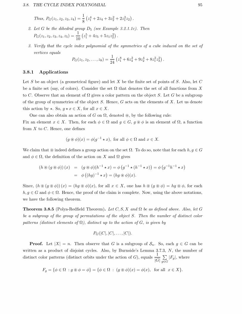
3.8. THE CYCLE INDEX POLYNOMIAL 95
Thus, PG(z1, z2, z3, z4) =1
8
(z41 + 2z4 + 3z22 + 2z21z2
).
2. Let G be the dihedral group D5 (see Example 3.2.1.1c). Then
PG(z1, z2, z3, z4, z5) =1
10
(z51 + 4z5 + 5z1z
22
).
3. Verify that the cycle index polynomial of the symmetries of a cube induced on the set of
vertices equals
PG(z1, z2, . . . , z8) =1
24
(z81 + 6z24 + 9z42 + 8z21z
23
).
3.8.1 Applications
Let S be an object (a geometrical figure) and let X be the finite set of points of S. Also, let C
be a finite set (say, of colors). Consider the set Ω that denotes the set of all functions from X
to C. Observe that an element of Ω gives a color pattern on the object S. Let G be a subgroup
of the group of symmetries of the object S. Hence, G acts on the elements of X. Let us denote
this action by ⋆. So, g ⋆ x ∈ X, for all x ∈ X.
One can also obtain an action of G on Ω, denoted ⊛, by the following rule:
Fix an element x ∈ X. Then, for each φ ∈ Ω and g ∈ G, g ⊛ φ is an element of Ω, a function
from X to C. Hence, one defines
(g ⊛ φ)(x) = φ(g−1 ⋆ x), for all φ ∈ Ω and x ∈ X.
We claim that ⊛ indeed defines a group action on the set Ω. To do so, note that for each h, g ∈ G
and φ ∈ Ω, the definition of the action on X and Ω gives
(h⊛ (g ⊛ φ)) (x) = (g ⊛ φ)(h−1 ⋆ x) = φ(g−1 ⋆ (h−1 ⋆ x)
)= φ
(g−1h−1 ⋆ x
)
= φ((hg)−1 ⋆ x
)= (hg ⊛ φ)(x).
Since, (h⊛ (g ⊛ φ)) (x) = (hg ⊛ φ)(x), for all x ∈ X, one has h ⊛ (g ⊛ φ) = hg ⊛ φ, for each
h, g ∈ G and φ ∈ Ω. Hence, the proof of the claim is complete. Now, using the above notations,
we have the following theorem.
Theorem 3.8.5 (Polya-Redfield Theorem). Let C,S,X and Ω be as defined above. Also, let G
be a subgroup of the group of permutations of the object S. Then the number of distinct color
patterns (distinct elements of Ω), distinct up to the action of G, is given by
PG(|C|, |C|, . . . , |C|).
Proof. Let |X| = n. Then observe that G is a subgroup of Sn. So, each g ∈ G can be
written as a product of disjoint cycles. Also, by Burnside’s Lemma 3.7.3, N , the number of
distinct color patterns (distinct orbits under the action of G), equals1
|G|∑
g∈G|Fg|, where
Fg = φ ∈ Ω : g ⊛ φ = φ = φ ∈ Ω : (g ⊛ φ)(x) = φ(x), for all x ∈ X.

96 CHAPTER 3. GROUPS AND POLYA THEORY
We claim that “g ∈ G fixes a color pattern (or an element of Ω) if and only if φ colors the
elements in a given cycle of g with the same color”.
Suppose that g ⊛ φ = φ. That is, (g ⊛ φ)(x) = φ(x), for all x ∈ X. So, using the definition,
one has φ(g−1 ⋆ x) = φ(x), for all x ∈ X. In particular, for a fixed x0 ∈ X, one also has
φ(x0) = φ(g ⋆ x0) = φ(g2 ⋆ x0
)= · · · .
Note that, for each fixed x0 ∈ X and g ∈ G, the permutation (x0, g⋆x0, g2 ⋆x0, . . .) corresponds
to a cycle of g. Therefore, if g fixes a color pattern φ, i.e., g ⊛ φ = φ, then φ assigns the same
color to each element of any cycle of g.
Conversely, fix an element g ∈ G and let φ be a color pattern (a function) that has the
property that every point in a given cycle of g is colored with the same color. That is, φ(x) =
φ(g ⋆ x), for each x ∈ X. Or equivalently, φ(x) = φ(g−1 ⋆ x
)= (g⊛ φ)(x), for all x ∈ X. Hence,
by definition, g ⊛ φ = φ. Thus, g fixes the color pattern φ. Hence, the proof of the claim is
complete.
Therefore, we observe that for a fixed g ∈ G, a cycle of g can be given a color independent
of another cycle of g. Also, the number of distinct colors equals |C|. Hence, using the principle
of basic counting (see Item 2 on Page 25), for a fixed g ∈ G, |Fg| = |C|ℓ1(g) · |C|ℓ2(g) · · · |C|ℓn(g),where for each k, 1 ≤ k ≤ n, ℓk(g) denotes the number of cycles of g of length k. Thus,
N =1
|G|∑
g∈G
|Fg| =1
|G|∑
g∈G
|C|ℓ1(g) · |C|ℓ2(g) · · · |C|ℓn(g) = PG(|C|, |C|, . . . , |C|).
We now give a few examples to indicate the importance of Theorem 3.8.5.
Example 3.8.6. 1. Determine the number of distinct color patterns, when the vertices of a
pentagon is colored with 3 colors.
Solution: It can be easily observed that the group D5, the group of symmetries of a
pentagon, acts on the color patterns. Now, verify that
PD5(z1, z2, . . . , z5) =1
|D5|(z51 + 4z5 + 5z1z
22) =
z51 + 4z5 + 5z1z22
10.
Thus, by Theorem 3.8.5, the required number equals N =1
10(35 + 4 · 3 + 5 · 3 · 32) = 39.
2. Suppose we are given beads of 3 different colors and that there are at least 6 beads of each
color. Determine the distinct necklace patterns that are possible using the 6 beads.
Solution: Since we are forming a necklace using 6 beads, the group D6 acts on the 6 beads
of the necklace. Also, the cycle index polynomial of D6 equals PD6(z1, z2, . . . , z5, z6) =1
|D6|(z61 + 2z6 + 2z23 + z32 + 3z32 + 3z21z
22). Hence, by Theorem 3.8.5, the number of distinct
necklace patterns equals1
12(36 + 2 · 3 + 2 · 32 + 4 · 33 + 3 · 32 · 32) = 92.

3.8. THE CYCLE INDEX POLYNOMIAL 97
3. Consider the 2 × 2 square given in Figure 3.7. Determine the number of distinct color
patterns, when the vertices of the given figure are colored with two colors.
Solution: Observe that D4 is the group of symmetries of the 2× 2 square and it needs to
act on 9 vertices. So, we need to write the elements of D4 as a subgroup of S9. Hence, the
cycle index polynomial is given by PD4(z1, . . . , z9) =z91 + 2z1z
24 + z1z
42 + 4z31z
32
8and the
number of distinct color patterns equals 102.
1 2 3
7 8 9
4 5 6
The 2× 2 Square
1 2 3 4
5 6 7 8
9 10 11 12
13 14 15 16
The 4× 4 Square
Figure 3.7: Faces and Vertices of Squares
4. Determine the number of distinct color patterns when the edges of a cube are colored with
2 colors.
Solution: Using the group of symmetries of the cube given on Page 77, the cycle index
polynomial corresponding to the faces equals PG(z1, . . . , z12) =z121 + 6z34 + 3z62 + 8z43 + 6z21z
52
24.
Thus, the required number is 218.

98 CHAPTER 3. GROUPS AND POLYA THEORY
3.9 Polya Inventory Theorem
In this section, the ideas of the previous subsection are generalized. This generalization allows
us to count the distinct number of necklaces even if there are not sufficient number of beads
of each color. To do this, each element of C is assigned a weight, that in turn gives weight to
each color pattern. This weight may be a number, a variable or in general, an element of a
commutative ring with identity. The setup for our study remains the same. To start with, we
have the following definitions.
Definition 3.9.1 (Weight of a color pattern). Let A be a commutative ring with identity (the
elements of A are called weights). Let w : C−→A be a map that assigns weights to each color.
Then, the weight of a color pattern φ : X−→C, with respect to the weight function w is given by
w(φ) =∏
x∈Xw(φ(x)
).
Fix g ∈ G. Then we have seen that g fixes a color pattern φ ∈ Ω if and only if φ colors the
elements in a given cycle of g with the same color. Similarly, for each fixed g ∈ G and φ ∈ Ω,
one has
w(g ⊛ φ) =∏
x∈X
w(g ⊛ φ(x)
)=∏
x∈X
w(φ(g−1 ⋆ x)
)=∏
y∈X
w(φ(y)
)= w(φ), (3.1)
as g⋆x : x ∈ X = X (see Remark 3.6.2). That is, for a fixed φ ∈ Ω, the weight of each element
of O(φ) = g ⊛ φ : g ∈ G is the same and it equals w(φ). That is, w(φ) = w(ψ), whenever
ψ = g ⊛ φ, for some g ∈ G.
Example 3.9.2. Let X consist of the set of faces of a cube, G be the group of symmetries of the
cube and let C consist of two colors ‘Red’ and ‘Blue’. Thus, if the weights R and B are assigned
to the two elements of C then the weight
1. B6 corresponds to “all faces being colored Blue”;
2. R2B4 corresponds to “any two faces being colored ‘Red’ and the remaining four faces being
colored ‘Blue’;
3. R3B3 corresponds to “any three faces being colored ‘Red’ and the remaining three faces
being colored ‘Blue’ and so on.
Example 3.9.2 indicates that different color patterns need not have different weights. We
also need the following definition to state and prove results in this area.
Definition 3.9.3 (Pattern Inventory). Let G be a group acting on the set Ω (the set of color
patterns) and let w : C−→A be a weight function. The pattern inventory, denoted I, under the
action of G on Ω, with respect to w, is the sum of the weights of the orbits. That is, I =∑
∆w(∆),
where the sum runs over all the distinct orbits ∆ obtained by the action of G on Ω.

3.9. POLYA INVENTORY THEOREM 99
With the above definitions, we are ready to prove the Polya’s Enumeration Theorem. To do
so, we first need to prove the weighted Burnside’s Lemma. This Lemma is the weighted version
of the Burnside’s Lemma 3.7.3.
Lemma 3.9.4. With the definitions and notations as above,
I =∑
∆
w(∆) =1
|G|∑
g∈G
∑
φ∈Ω
g⊛φ=φ
w(φ),
where the sum runs over all the distinct orbits ∆ obtained by the action of G on Ω.
Proof. As G acts on Ω, for each α ∈ Ω, the application of Lemma 3.6.7 gives |Gα| · |O(α)| =|G|. Since ∆ is an orbit under the action of G, for each φ ∈ ∆, |Gφ| · |∆| = |G|. Also, by
definition, w(∆) = w(φ), for all φ ∈ ∆. Thus,
w(∆) = w(φ) =1
|∆|∑
φ∈∆
w(φ) =∑
φ∈∆
1
|∆|w(φ) =∑
φ∈∆
|Gφ||G| w(φ) =
1
|G|∑
φ∈∆
|Gφ| · w(φ).
Let Fg = φ ∈ Ω : g ⊛ φ = φ. Then ∑
φ∈Ω
∑
g∈Gφ
w(φ) =∑
g∈G
∑
φ∈Fg
w(φ) and hence
I =∑
∆
w(∆) =∑
∆
1
|G|∑
φ∈∆
|Gφ| · w(φ) =1
|G|∑
∆
∑
φ∈∆
|Gφ| · w(φ) =1
|G|∑
φ∈Ω
|Gφ| · w(φ)
=1
|G|∑
φ∈Ω
∑
g∈Gφ
w(φ) =1
|G|∑
g∈G
∑
φ∈Fg
w(φ).
We are now in a position to prove the Polya’s Enumeration Theorem. Before doing so, recall
that Fg consists precisely of those color schemes which color each cycle of g with just one color
(see the argument used in the second paragraph in the proof of Theorem 3.8.5).
Theorem 3.9.5 (Polya’s Enumeration Theorem). With the definitions and notations as above,
I =∑
∆
w(∆) = PG(x1, x2, . . . , xn),
where the sum runs over all the distinct orbits ∆ obtained by the action of G on Ω and xi =∑
c∈Cw(c)i, is the ith power sum of the weights of the colors. In particular, if weight of each color
is 1, I = PG(|C|, |C|, . . . , |C|).
Proof. Using the weighted Burnside Lemma 3.9.4, we need to prove that
∑
g∈G
∑
φ∈Fg
w(φ) =∑
g∈G
xℓ1(g)1 x
ℓ2(g)2 · · · xℓn(g)n ,
where ℓi(g) is the number of cycles of length i in the cycle representation of g.
Now, fix a g ∈ G. Suppose g has exactly t disjoint cycles, say g1, g2, . . . , gt. As Fg consists
precisely of those color schemes which color each cycle of g with just one color, we just need

100 CHAPTER 3. GROUPS AND POLYA THEORY
to determine the weight of such a color pattern. To do so, for 1 ≤ i ≤ t, define Xi to be that
subset of X whose elements form the cycle gi. Then, it is easy to see that X1,X2, . . . ,Xt defines
a partition of X. Also, the condition that x and g ⋆x belong to the same cycle of g, implies that
w(φ(si)) = w(φ(g ⋆ si)), for each si ∈ Xi, 1 ≤ i ≤ t. Thus, for each φ ∈ Fg,
w(φ) =∏
x∈X
w(φ(x)) =
t∏
i=1
∏
x∈Xi
w(φ(x)) =
t∏
i=1
w(φ(si))|Xi|.
Note that if we pick a term from each factor int∏
i=1
(∑
c∈Cw(c)|Xi|
)
and take the product of
these terms, we obtain all the terms oft∏
i=1
(∑
c∈Cw(c)|Xi|
)
. All these terms also appear in
∑
φ∈Fg
t∏
i=1w(φ(si))
|Xi| because as φ is allowed to vary over all elements of Fg, the images φ(si), for
1 ≤ i ≤ t, take all values in C. The argument can also be reversed and hence it follows that
∑
φ∈Fg
w(φ) =∑
φ∈Fg
t∏
i=1
w(φ(si))|Xi| =
t∏
i=1
(∑
c∈C
w(c)|Xi|
)
.
Now, assume that g has ℓk(g) cycles of length k, 1 ≤ k ≤ n. This means that in the
collection |X1|, |X2|, . . . , |Xt|, the number 1 appears ℓ1(g) times, the number 2 appears ℓ2(g)
times and so on till the number n appears ℓn(g) times (note that some of the ℓi(g)’s may be
zero). Consequently,t∏
i=1
(∑
c∈C
w(c)|Xi|
)
equalsn∏
k=1
xℓk(g)k , as x1 =
∑
c∈C
w(c), x2 =∑
c∈C
w(c)2 and
so on till xn =∑
c∈Cw(c)n. Hence,
∑
φ∈Fg
w(φ) =n∏
k=1
xℓk(g)k and thus, the required result follows.
Example 3.9.6. 1. Consider a necklace consisting of 6 beads. If there are 3 color choices,
say R,B and G, then determine
(a) the number of necklaces that have at least one R bead.
(b) the number of necklaces that have three R, two B and one G bead.
Solution: Recall that D6 acts on a regular hexagon and its cycle index polynomial equals
PD6(z1, z2, . . . , z6) =1
12(z61 + 4z32 + 2z23 + 2z6 + 3z21z
22).
So, for the first part, at least one R needs to be used and the remaining can be any number
of B and/or G. So, we define the weight of the color R as x and that of B and G as 1.
Therefore, by Polya’s Enumeration Theorem 3.9.5,
I =1
12
((x+ 1 + 1)6 + 4(x2 + 1 + 1)3 + 2(x3 + 1 + 1)2
+2(x6 + 1 + 1) + 3(x+ 1 + 1)2(x2 + 1 + 1)2)
= x6 + 2x5 + 9x4 + 16x3 + 29x2 + 20x + 15.

3.9. POLYA INVENTORY THEOREM 101
So, the required answer is 1 + 2 + 9 + 16 + 29 + 20 = 77.
For the second part, define the weights as R,B and G itself. Then
I =1
12
((R+B +G)6 + 4(R2 +B2 +G2)3 + 2(R3 +B3 +G3)2
+2(R6 +B6 +G6) + 3(R +B +G)2(R2 +B2 +G2)2).
The required answer equals the coefficient of R3B2G in I, which equals
1
12
((6
3, 2, 1
)
+ 3 · 2 · 2)
=1
12
(6!
3!2!+ 6
)
= 6.
We end this chapter with a few Exercises. But before doing so, we give the following example
with which Polya started his classic paper on this subject.
Example 3.9.7. Suppose we are given 6 similar spheres in three different colors, say, three Red,
two Blue and one Yellow (spheres of the same color being indistinguishable). In how many ways
can we distribute the six spheres on the 6 vertices of an octahedron freely movable in space?
Solution: Here X = 1, 2, 3, 4, 5, 6 and C = R,B, Y . Using Example 3.2.1.2b on Page 77
the cycle index polynomial corresponding to the symmetric group of the octahedron that acts on
the vertices of the octahedron is given by
1
24
(z61 + 6z21z4 + 3z21z
22 + 8z23 + 6z32
).
Hence, the number of patterns of the required type is the coefficient of the term R3B2Y in
I =1
24
((R+B + Y )6 + 6(R +B + Y )2(R4 +B4 + Y 4) + 3(R +B + Y )2(R2 +B2 + Y 2)2
+8(R3 +B3 + Y 3)2 + 6(R2 +B2 + Y 2)3).
Verify that this number equals 3.
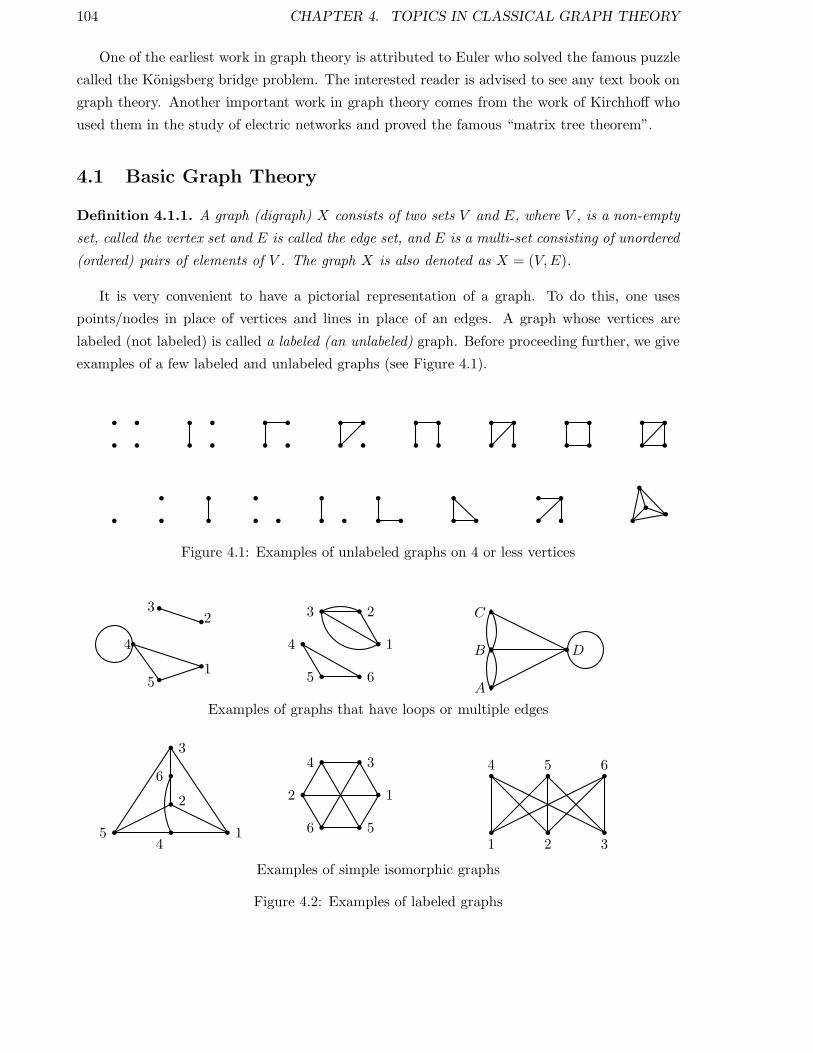
104 CHAPTER 4. TOPICS IN CLASSICAL GRAPH THEORY
One of the earliest work in graph theory is attributed to Euler who solved the famous puzzle
called the Konigsberg bridge problem. The interested reader is advised to see any text book on
graph theory. Another important work in graph theory comes from the work of Kirchhoff who
used them in the study of electric networks and proved the famous “matrix tree theorem”.
4.1 Basic Graph Theory
Definition 4.1.1. A graph (digraph) X consists of two sets V and E, where V , is a non-empty
set, called the vertex set and E is called the edge set, and E is a multi-set consisting of unordered
(ordered) pairs of elements of V . The graph X is also denoted as X = (V,E).
It is very convenient to have a pictorial representation of a graph. To do this, one uses
points/nodes in place of vertices and lines in place of an edges. A graph whose vertices are
labeled (not labeled) is called a labeled (an unlabeled) graph. Before proceeding further, we give
examples of a few labeled and unlabeled graphs (see Figure 4.1).
Figure 4.1: Examples of unlabeled graphs on 4 or less vertices
1
23
4
5
Examples of graphs that have loops or multiple edges
14
23
65A
B
C
D
1 2 3
4 5 6
Examples of simple isomorphic graphs
12
34
56154
2
6
3
Figure 4.2: Examples of labeled graphs
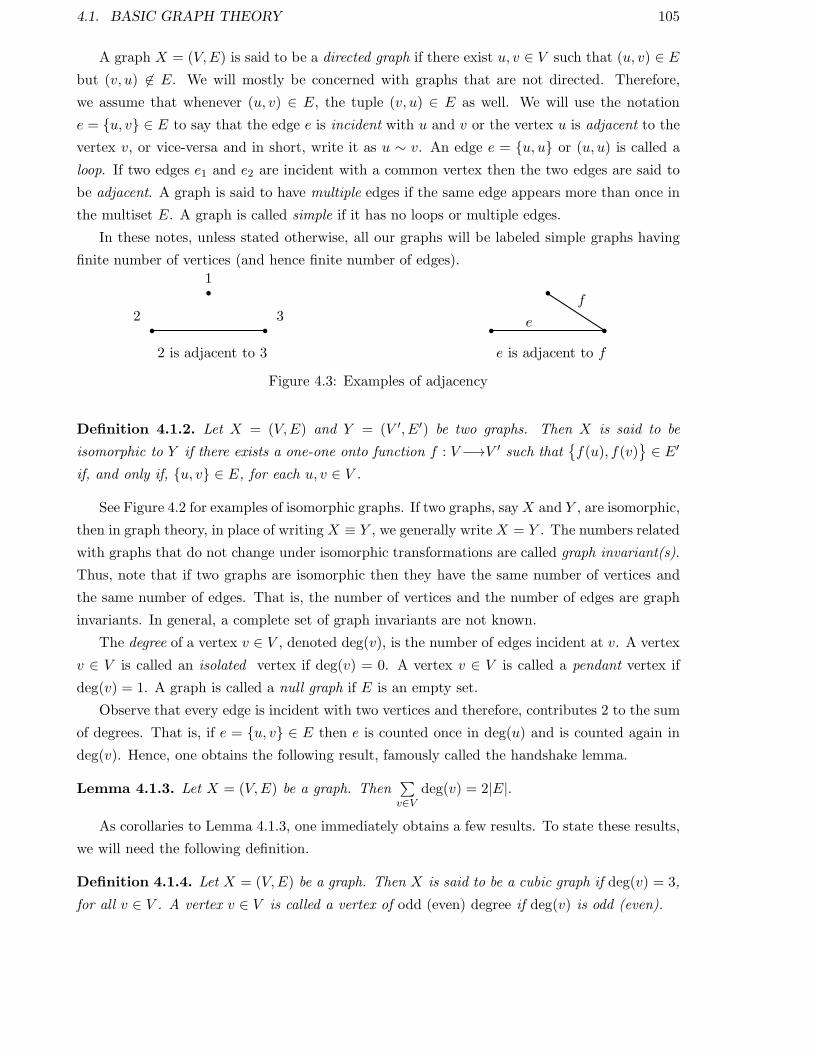
4.1. BASIC GRAPH THEORY 105
A graph X = (V,E) is said to be a directed graph if there exist u, v ∈ V such that (u, v) ∈ E
but (v, u) 6∈ E. We will mostly be concerned with graphs that are not directed. Therefore,
we assume that whenever (u, v) ∈ E, the tuple (v, u) ∈ E as well. We will use the notation
e = u, v ∈ E to say that the edge e is incident with u and v or the vertex u is adjacent to the
vertex v, or vice-versa and in short, write it as u ∼ v. An edge e = u, u or (u, u) is called a
loop. If two edges e1 and e2 are incident with a common vertex then the two edges are said to
be adjacent. A graph is said to have multiple edges if the same edge appears more than once in
the multiset E. A graph is called simple if it has no loops or multiple edges.
In these notes, unless stated otherwise, all our graphs will be labeled simple graphs having
finite number of vertices (and hence finite number of edges).
1
2 3
2 is adjacent to 3
e
f
e is adjacent to f
Figure 4.3: Examples of adjacency
Definition 4.1.2. Let X = (V,E) and Y = (V ′, E′) be two graphs. Then X is said to be
isomorphic to Y if there exists a one-one onto function f : V−→V ′ such thatf(u), f(v)
∈ E′
if, and only if, u, v ∈ E, for each u, v ∈ V .
See Figure 4.2 for examples of isomorphic graphs. If two graphs, sayX and Y , are isomorphic,
then in graph theory, in place of writingX ≡ Y , we generally write X = Y . The numbers related
with graphs that do not change under isomorphic transformations are called graph invariant(s).
Thus, note that if two graphs are isomorphic then they have the same number of vertices and
the same number of edges. That is, the number of vertices and the number of edges are graph
invariants. In general, a complete set of graph invariants are not known.
The degree of a vertex v ∈ V , denoted deg(v), is the number of edges incident at v. A vertex
v ∈ V is called an isolated vertex if deg(v) = 0. A vertex v ∈ V is called a pendant vertex if
deg(v) = 1. A graph is called a null graph if E is an empty set.
Observe that every edge is incident with two vertices and therefore, contributes 2 to the sum
of degrees. That is, if e = u, v ∈ E then e is counted once in deg(u) and is counted again in
deg(v). Hence, one obtains the following result, famously called the handshake lemma.
Lemma 4.1.3. Let X = (V,E) be a graph. Then∑
v∈Vdeg(v) = 2|E|.
As corollaries to Lemma 4.1.3, one immediately obtains a few results. To state these results,
we will need the following definition.
Definition 4.1.4. Let X = (V,E) be a graph. Then X is said to be a cubic graph if deg(v) = 3,
for all v ∈ V . A vertex v ∈ V is called a vertex of odd (even) degree if deg(v) is odd (even).
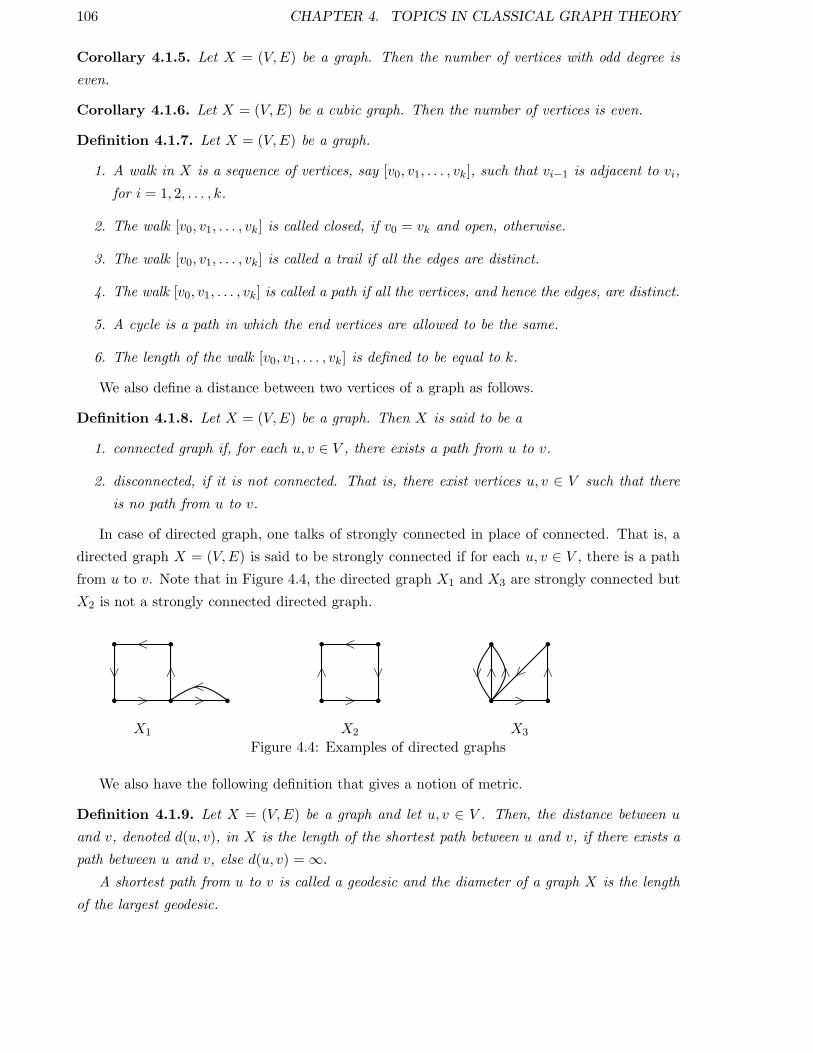
106 CHAPTER 4. TOPICS IN CLASSICAL GRAPH THEORY
Corollary 4.1.5. Let X = (V,E) be a graph. Then the number of vertices with odd degree is
even.
Corollary 4.1.6. Let X = (V,E) be a cubic graph. Then the number of vertices is even.
Definition 4.1.7. Let X = (V,E) be a graph.
1. A walk in X is a sequence of vertices, say [v0, v1, . . . , vk], such that vi−1 is adjacent to vi,
for i = 1, 2, . . . , k.
2. The walk [v0, v1, . . . , vk] is called closed, if v0 = vk and open, otherwise.
3. The walk [v0, v1, . . . , vk] is called a trail if all the edges are distinct.
4. The walk [v0, v1, . . . , vk] is called a path if all the vertices, and hence the edges, are distinct.
5. A cycle is a path in which the end vertices are allowed to be the same.
6. The length of the walk [v0, v1, . . . , vk] is defined to be equal to k.
We also define a distance between two vertices of a graph as follows.
Definition 4.1.8. Let X = (V,E) be a graph. Then X is said to be a
1. connected graph if, for each u, v ∈ V , there exists a path from u to v.
2. disconnected, if it is not connected. That is, there exist vertices u, v ∈ V such that there
is no path from u to v.
In case of directed graph, one talks of strongly connected in place of connected. That is, a
directed graph X = (V,E) is said to be strongly connected if for each u, v ∈ V , there is a path
from u to v. Note that in Figure 4.4, the directed graph X1 and X3 are strongly connected but
X2 is not a strongly connected directed graph.
>
>
>
>
<
>
X1
>
>
<
>
X2
>
>>
>
X3
>
>
Figure 4.4: Examples of directed graphs
We also have the following definition that gives a notion of metric.
Definition 4.1.9. Let X = (V,E) be a graph and let u, v ∈ V . Then, the distance between u
and v, denoted d(u, v), in X is the length of the shortest path between u and v, if there exists a
path between u and v, else d(u, v) = ∞.
A shortest path from u to v is called a geodesic and the diameter of a graph X is the length
of the largest geodesic.

4.1. BASIC GRAPH THEORY 107
With the definitions as above, one has the following result in graph theory.
Proposition 4.1.10. Let X = (V,E) be a non-null graph. Then X is disconnected if and only
if the vertex set V can be partitioned into two parts, say V1, V2, such that if e = u, v ∈ E then
either both u, v ∈ V1 or both u, v ∈ V2.
Proof. Let us assume that there exists a partition of V into two parts, say V1 and V2, satisfying
the properties stated in the proposition. Since V1 and V2 are non-empty, there exists u ∈ V1
and v ∈ V2. We claim that there is no path in X joining the vertices u and v. For if, there is a
path from u to v, then there will be at least one edge, say e = x, y ∈ E such that x ∈ V1 and
y ∈ V2. This contradicts the assumption that either both x, y ∈ V1 or both x, y ∈ V2.
Conversely, let us assume that X is a disconnected graph. Now, fix a vertex, say u ∈ V
and define V1 = x ∈ V : d(u, x) < ∞. Since X is disconnected V1 V and hence the set
V2 = V \ V1 is a non-empty subset of V . Clearly the two sets V1 and V2 give a partition of V
and there is no edge joining a vertex in V1 with a vertex in V2. Hence, this completes the proof
of the proposition.
We end this section, with a small list of well known graphs and a set of exercises.
Definition 4.1.11. 1. Let X = (V,E) be a graph on |V | = n vertices, with V = v1, v2, . . . , vn.Then X is said to be a
(a) null graph, denoted 0n, if E = ∅.(b) path graph, denoted Pn, if E = vi, vi+1 : 1 ≤ i ≤ n− 1.(c) cycle graph, denoted Cn, if E = vi, vi+1 : 1 ≤ i ≤ n− 1 ∪ v1, vn.(d) tree if X is connected and has no cycle.
(e) complete graph, denoted Kn, if E = vi, vj : 1 ≤ i < j ≤ n.(f) d-regular graph if deg(vi) = d for all i = 1, 2, . . . , n. Note that a cycle graph is a
2-regular graph, whereas the complete graph Kn is a (n− 1)-regular graph.
2. A graph X = (V,E) is said to be a bipartite graph, if V is a disjoint union of two sets, say
V1 and V2 such that every edge of X is incident with a vertex in V1 and the other with a
vertex in V2.
3. A graph X = (V,E) is said to be a complete bipartite graph, if V = v1, . . . , vm, u1, . . . , unand E = vi, uj : 1 ≤ i ≤ m, 1 ≤ j ≤ n. This graph is denoted by Km,n.

108 CHAPTER 4. TOPICS IN CLASSICAL GRAPH THEORY
1
P1
1 2
P2
2
1
3
P3
1
4
2
3
P4
3
2
4
1
5
P5
1
K1
1 2
K2
2
1
3
K3
1
4
2
3
K4
1
23
4
5K5
2
1
3
C3
1
4
2
3
C4
1
23
4
5C5
15
42
63C6
1 2
K1,1
2
1
3
K1,2
1
4
2
3
K2,2
1 2 3
4 5
K2,3
Figure 4.5: Some well known family of graphs
4.2 Graph Operations
A graph Y = (V ′, E′) is said to be a subgraph of a graph X = (V,E) if V ′ ⊂ V and E′ ⊂ E.
One also states this by saying that the graph X is a supergraph of the graph Y . A subgraph
Y = (V ′, E′) of X = (V,E) is said to be a spanning subgraph if V ′ = V and is called an induced
subgraph if, for each u, v ∈ V ′ ⊂ V , the edge u, v ∈ E′ whenever u, v ∈ E. In this case, the
set V ′ is said to induce the subgraph Y and this is denoted by writing Y = X[V ′]. With the
definitions as above, one observes the following:
1. Every graph is its own subgraph.
2. If Z is a subgraph of Y and Y is a subgraph of X then Z is also a subgraph of X.
3. A single vertex of a graph is also its subgraph.
4. A single edge of a graph together with its incident vertices is also its subgraph.
We also have the following graph operations.
Definition 4.2.1. 1. Let X1 = (V1, E1) and X2 = (V2, E2) be two graphs. Then the
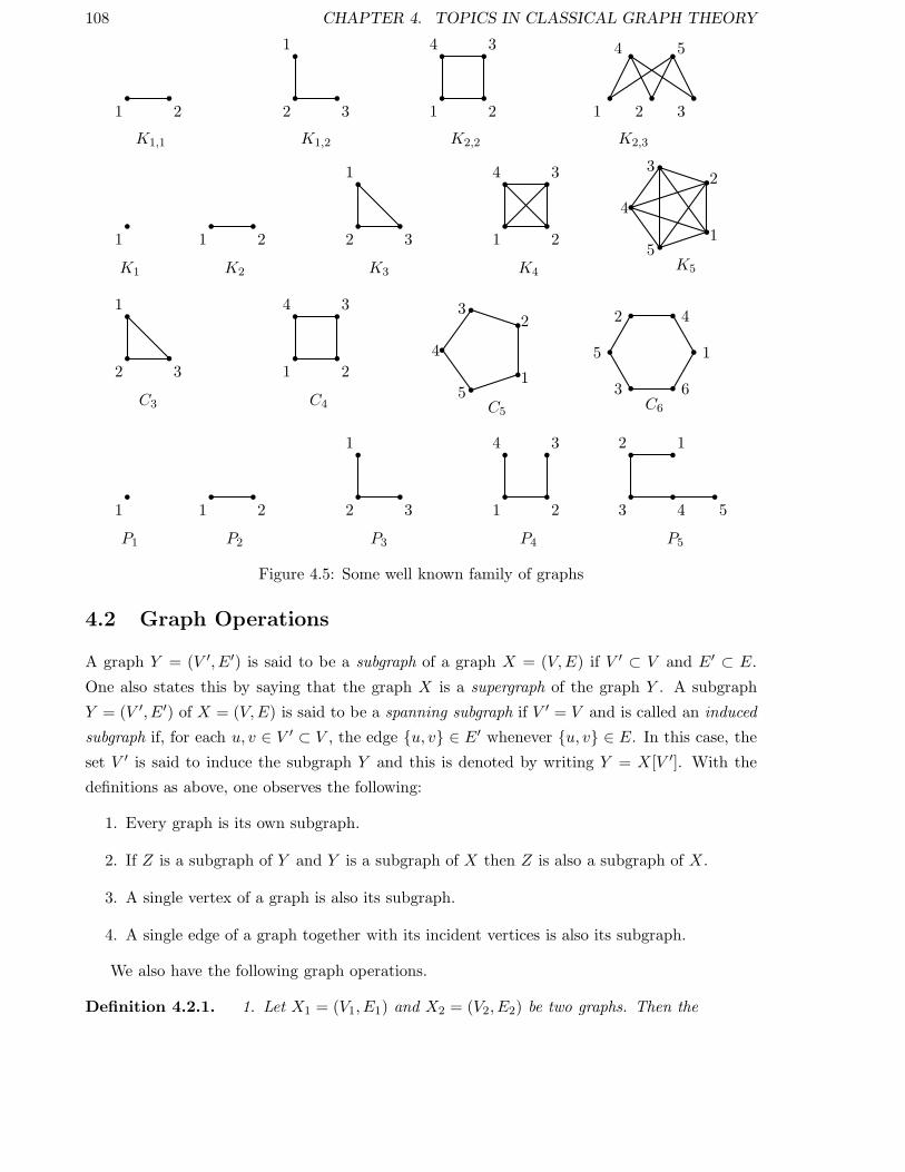

4.2. GRAPH OPERATIONS 109
(a) union of X1 and X2, denoted X1 ∪X2, is a graph whose vertex set is V1 ∪ V2 and the
edge set is E1 ∪ E2.
(b) intersection of X1 and X2, denoted X1 ∩X2, is a graph whose vertex set is V1 ∩ V2and the edge set is E1 ∩E2.
2. Let X = (V,E) be a graph and fix a subset U ⊂ V and F ⊂ E. Then
(a) X \ U denotes a subgraph of X that is obtained by removing all the vertices v ∈ U
from X and all edges that are incident with some vertex v ∈ U .
(b) X \ F denotes a subgraph of X that is obtained by the removal of each edge e ∈ F .
Thus, note that X \F is a spanning subgraph of X, whereas X \U is an induced subgraph
of X on the vertex set V \ U . If U = v and F = e, then one writes X \ v in place of
X \ v and X \ e in place of X \ e.
3. Let X = (V,E) be a graph and let v be a vertex such that v 6∈ V . Also, suppose that there
exist x, y ∈ V such that e = x, y 6∈ E. Then
(a) X + v is a graph that is obtained from X by including the vertex v and joining it
to all other vertices of X. That is, X + v = (V ′, E′), where V ′ = V ∪ v and
E′ = E ∪ v, u : u ∈ V .
(b) X + e is a graph that is obtained from X by joining the edge e. That is, X + e =
(V ′, E′), where V ′ = V and E′ = E ∪ e.
(c) Let X = (V,E) and Y = (V ′, E′) be two graphs with V ∩ V ′ = ∅. Then the
i. join of X and Y , denoted X + Y = (V1, E1), is a graph having V1 = V ∪ V ′ and
E1 = E ∪E′ ∪ u, v : u ∈ V, v ∈ V ′.ii. cartesian product of X and Y , denoted X × Y = (V1, E1), is a graph having
V1 = V ×V ′ and whose edge set consists of all elements (u1, u2), (v1, v2), whereeither u1 = v1 and u2, v2 ∈ E′ or u2 = v2 and u1, v1 ∈ E.
See Figure 4.6 for examples related to the above graph operations.
The graph operations defined above lead to the concepts of what are called connected com-
ponents, cut-vertices, cut-edge/bridges and blocks in a graph. We define them now.
Definition 4.2.2. Let X = (V,E) be a graph. Then
1. a connected component (or in short component) of X is a connected induced subgraph
Y = (V ′, E′) of X such that if Z is any connected subgraph of X that has Y as its
subgraph then Y = Z.
2. a vertex v ∈ V is called a cut-vertex if the number of components in X \ v increases.

110 CHAPTER 4. TOPICS IN CLASSICAL GRAPH THEORY
a
b
X
1 2 3
Y
1a 2a 3a
1b 2b 3b
X × Y
11 21 31
1222
32
13 23 33
Y × Y
1
4
2
3
X2 = X1 \ 1, 3, 2, 4NOT an induced subgraph of X1
1
4
2
3
X1 = K2 +K2
1
23
4
5X3 = X1 + 5
1
4
2
3
X5 = X2 ∩X4
1 2 3
4 5 6
X4
1 2 3
4 5 6
X6 = X1 ∪X4
Figure 4.6: Examples of graph operations
3. an edge e ∈ E is called a cut-edge/bridge if the number of components in X \ e increases.
4. a block of X is a maximal induced connected subgraph of X having no cut-vertex.
5. a clique of X is a maximal induced complete subgraph of X.
We also need the following important definitions related with graph operations.
Definition 4.2.3. Let X = (V,E) be a graph with |V | = n. Then
1. the complement graph of X is the graph Y = (V ′, E′), denoted X, such that V ′ = V and
E′ = E(Kn) \E, where E(Kn) is the edge set of the complete graph Kn.
2. the line graph of X is the graph Y = (V ′, E′), denoted L(X), such that V ′ = E and any
two elements of V ′ are joined by an edge if they have a common vertex of X incident to
them.
See Figure 4.8 for examples of line and complement graphs. Observe that if X = (V,E)
is the complement of the graph Y = (V ′, E′) then V = V ′. If |V | = n, then the set E can
be obtained by removing those edges of Kn that are also edges of Y . In other words, the two
graphs are complementary to each other. A graph X is said to be self-complementary if X = X .
For example, the path P4, on 4 vertices, and the cycle C5, on 5 vertices, are self-complementary
graphs.
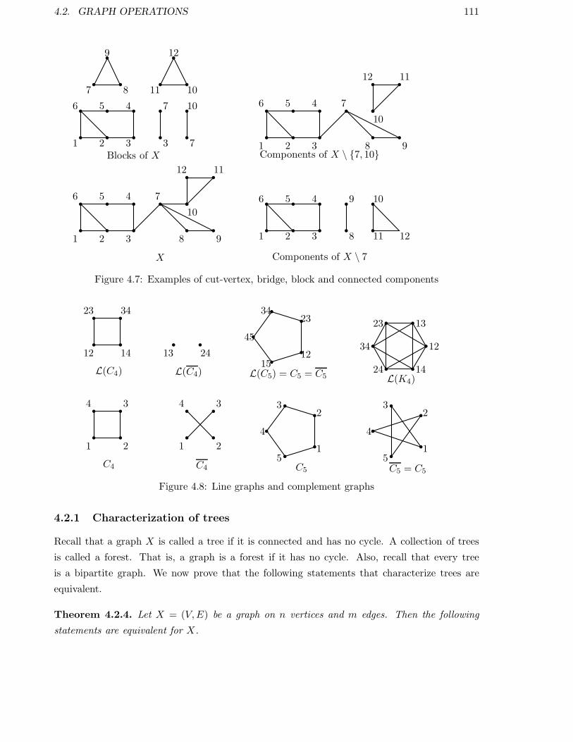
4.2. GRAPH OPERATIONS 111
1 2 3
456 7
8 9
10
1112
X
1 2 3
456
3
7
7
10
7 8
9
1011
12
Blocks of X
1 2 3
456
8
9
11
10
12
Components of X \ 7
1 2 3
456 7
8 9
10
1112
Components of X \ 7, 10
Figure 4.7: Examples of cut-vertex, bridge, block and connected components
1
4
2
3
C4
1
4
2
3
C4
1
23
4
5C5
1
23
4
5C5 = C5
12
23
14
34
L(C4)
13 24
L(C4)
12
2334
45
15L(C5) = C5 = C5
1234
1323
1424L(K4)
Figure 4.8: Line graphs and complement graphs
4.2.1 Characterization of trees
Recall that a graph X is called a tree if it is connected and has no cycle. A collection of trees
is called a forest. That is, a graph is a forest if it has no cycle. Also, recall that every tree
is a bipartite graph. We now prove that the following statements that characterize trees are
equivalent.
Theorem 4.2.4. Let X = (V,E) be a graph on n vertices and m edges. Then the following
statements are equivalent for X.
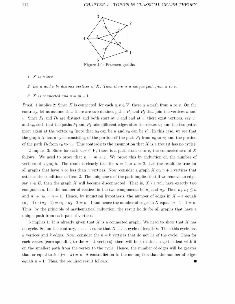
112 CHAPTER 4. TOPICS IN CLASSICAL GRAPH THEORY
1
2
3
4
5
a
bc
d
e
Figure 4.9: Petersen graphs
1. X is a tree.
2. Let u and v be distinct vertices of X. Then there is a unique path from u to v.
3. X is connected and n = m+ 1.
Proof. 1 implies 2: Since X is connected, for each u, v ∈ V , there is a path from u to v. On the
contrary, let us assume that there are two distinct paths P1 and P2 that join the vertices u and
v. Since P1 and P2 are distinct and both start at u and end at v, there exist vertices, say u0
and v0, such that the paths P1 and P2 take different edges after the vertex u0 and the two paths
meet again at the vertex v0 (note that u0 can be u and v0 can be v). In this case, we see that
the graph X has a cycle consisting of the portion of the path P1 from u0 to v0 and the portion
of the path P2 from v0 to u0. This contradicts the assumption that X is a tree (it has no cycle).
2 implies 3: Since for each u, v ∈ V , there is a path from u to v, the connectedness of X
follows. We need to prove that n = m + 1. We prove this by induction on the number of
vertices of a graph. The result is clearly true for n = 1 or n = 2. Let the result be true for
all graphs that have n or less than n vertices. Now, consider a graph X on n + 1 vertices that
satisfies the conditions of Item 2. The uniqueness of the path implies that if we remove an edge,
say e ∈ E, then the graph X will become disconnected. That is, X \ e will have exactly two
components. Let the number of vertices in the two components be n1 and n2. Then n1, n2 ≤ n
and n1 + n2 = n + 1. Hence, by induction hypothesis, the number of edges in X − e equals
(n1−1)+(n2−1) = n1+n2−2 = n−1 and hence the number of edges in X equals n−1+1 = n.
Thus, by the principle of mathematical induction, the result holds for all graphs that have a
unique path from each pair of vertices.
3 implies 1: It is already given that X is a connected graph. We need to show that X has
no cycle. So, on the contrary, let us assume that X has a cycle of length k. Then this cycle has
k vertices and k edges. Now, consider the n − k vertices that do not lie of the cycle. Then for
each vertex (corresponding to the n− k vertices), there will be a distinct edge incident with it
on the smallest path from the vertex to the cycle. Hence, the number of edges will be greater
than or equal to k + (n − k) = n. A contradiction to the assumption that the number of edges
equals n− 1. Thus, the required result follows.
4.2. GRAPH OPERATIONS 113
As a next result in this direction, we prove that a tree has at least two pendant (end) vertices.
Theorem 4.2.5. Let X be a non-trivial tree. Then X has at least two vertices of degree 1.
Proof. Let X = (V,E) with |V | = n ≥ 2. Then, by Theorem 4.2.4, |E| = n − 1. Also, by
handshake lemma (Lemma 4.1.3), we know that 2|E| = ∑
v∈Vdeg(v). Thus, 2(n−1) =
n∑
i=1deg(vi).
Now, X is connected implies that deg(v) ≥ 1, for all v ∈ V and hence the above equality implies
that there are at least two vertices for which deg(v) = 1. This ends the proof of the result.
For more results on trees, see the book graph theory by Harary [6].
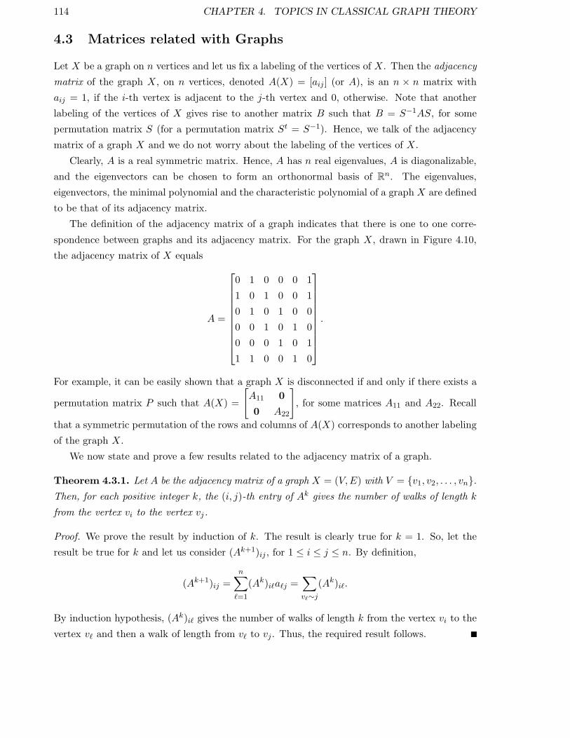
114 CHAPTER 4. TOPICS IN CLASSICAL GRAPH THEORY
4.3 Matrices related with Graphs
Let X be a graph on n vertices and let us fix a labeling of the vertices of X. Then the adjacency
matrix of the graph X, on n vertices, denoted A(X) = [aij ] (or A), is an n × n matrix with
aij = 1, if the i-th vertex is adjacent to the j-th vertex and 0, otherwise. Note that another
labeling of the vertices of X gives rise to another matrix B such that B = S−1AS, for some
permutation matrix S (for a permutation matrix St = S−1). Hence, we talk of the adjacency
matrix of a graph X and we do not worry about the labeling of the vertices of X.
Clearly, A is a real symmetric matrix. Hence, A has n real eigenvalues, A is diagonalizable,
and the eigenvectors can be chosen to form an orthonormal basis of Rn. The eigenvalues,
eigenvectors, the minimal polynomial and the characteristic polynomial of a graph X are defined
to be that of its adjacency matrix.
The definition of the adjacency matrix of a graph indicates that there is one to one corre-
spondence between graphs and its adjacency matrix. For the graph X, drawn in Figure 4.10,
the adjacency matrix of X equals
A =
0 1 0 0 0 1
1 0 1 0 0 1
0 1 0 1 0 0
0 0 1 0 1 0
0 0 0 1 0 1
1 1 0 0 1 0
.
For example, it can be easily shown that a graph X is disconnected if and only if there exists a
permutation matrix P such that A(X) =
[
A11 0
0 A22
]
, for some matrices A11 and A22. Recall
that a symmetric permutation of the rows and columns of A(X) corresponds to another labeling
of the graph X.
We now state and prove a few results related to the adjacency matrix of a graph.
Theorem 4.3.1. Let A be the adjacency matrix of a graph X = (V,E) with V = v1, v2, . . . , vn.Then, for each positive integer k, the (i, j)-th entry of Ak gives the number of walks of length k
from the vertex vi to the vertex vj .
Proof. We prove the result by induction of k. The result is clearly true for k = 1. So, let the
result be true for k and let us consider (Ak+1)ij , for 1 ≤ i ≤ j ≤ n. By definition,
(Ak+1)ij =
n∑
ℓ=1
(Ak)iℓaℓj =∑
vℓ∼j
(Ak)iℓ.
By induction hypothesis, (Ak)iℓ gives the number of walks of length k from the vertex vi to the
vertex vℓ and then a walk of length from vℓ to vj . Thus, the required result follows.
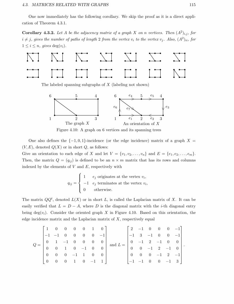
4.3. MATRICES RELATED WITH GRAPHS 115
One now immediately has the following corollary. We skip the proof as it is a direct appli-
cation of Theorem 4.3.1.
Corollary 4.3.2. Let A be the adjacency matrix of a graph X on n vertices. Then (A2)i,j , for
i 6= j, gives the number of paths of length 2 from the vertex vi to the vertex vj . Also, (A2)ii, for
1 ≤ i ≤ n, gives deg(vi).
The labeled spanning subgraphs of X (labeling not shown)
1 2 3
456
The graph X An orientation of X1 2 3
456
e1 e2
e4 e5
e3e6 e7
> <
> >
> <<
Figure 4.10: A graph on 6 vertices and its spanning trees
One also defines the −1, 0, 1-incidence (or the edge incidence) matrix of a graph X =
(V,E), denoted Q(X) or in short Q, as follows:
Give an orientation to each edge of X and let V = v1, v2, . . . , vn and E = e1, e2, . . . , em.Then, the matrix Q = (qij) is defined to be an n × m matrix that has its rows and columns
indexed by the elements of V and E, respectively with
qij =
1 ej originates at the vertex vi,
−1 ej terminates at the vertex vi,
0 otherwise.
The matrix QQt, denoted L(X) or in short L, is called the Laplacian matrix of X. It can be
easily verified that L = D − A, where D is the diagonal matrix with the i-th diagonal entry
being deg(vi). Consider the oriented graph X in Figure 4.10. Based on this orientation, the
edge incidence matrix and the Laplacian matrix of X, respectively equal
Q =
1 0 0 0 0 1 0
−1 −1 0 0 0 0 −1
0 1 −1 0 0 0 0
0 0 1 0 −1 0 0
0 0 0 −1 1 0 0
0 0 0 1 0 −1 1
and L =
2 −1 0 0 0 −1
−1 3 −1 0 0 −1
0 −1 2 −1 0 0
0 0 −1 2 −1 0
0 0 0 −1 2 −1
−1 −1 0 0 −1 3
.

116 CHAPTER 4. TOPICS IN CLASSICAL GRAPH THEORY
Note that depending on the orientation of the graph X, the incidence matrices may differ,
but there is no change in its Laplacian matrix. Hence, there is again a one to one correspondence
between the Laplacian matrix and the corresponding graph.
Let X be a graph on n vertices and let L be its Laplacian matrix. Then note that if we
add the 2-nd, 3-rd and so on till n-th row of L to the first row of L then the first row of L
equals the zero vector. Hence, det(L) = 0. A similar statement is true for the columns as
L is a symmetric matrix. The above argument also implies that 0 is an eigenvalue of L with
corresponding eigenvector e = (1, 1, . . . , 1)t. Also, L = QQt and hence L is a positive semi-
definite matrix. That is, all the eigenvalues of L are non-negative and there is a non-zero vector
x0 such that xt0Lx0 = 0. Using a result in matrix theory, it can be easily shown that the graph
X is disconnected if and only if the multiplicity of the eigenvalue 0 is at least 2.

4.4. MATRIX TREE THEOREM 117
4.4 Matrix Tree Theorem
We will now state a result in matrix theory, called the Cauchy Binet Theorem, and use it to
prove the famous theorem called the Matrix-Tree Theorem (Kirchhoff 1847). To do so, note that
for an m × n matrix A and S ⊂ 1, 2, . . . ,m, T ⊂ 1, 2, . . . , n, the notation A[S|T ] denotesthe sub-matrix of A that is determined by the rows that correspond to the elements of S and
the columns that correspond to the elements of T . For example, if
A =
1 2 1 3 4
2 1 3 1 0
1 2 4 4 1
and B =
[
2 1 4
2 4 1
]
then B = A[1, 3 | 2, 3, 5]. Also, the notation A(S|T ) corresponds to the matrix A[Sc|T c],
where for any subset W of Z, W c denotes the complement of W in Z. Thus,
A(1, 3 | 2, 3, 5) = A[2|1, 4] =[
2 1]
.
We also write A[i|j] and (A(i|j)) in place of A[i|j] and (A(i|j)).We now use the above notation to prove a result related to the edge incidence matrix of a
connected graph.
Lemma 4.4.1. Let X be a connected graph on n vertices and m edges. Also, let Q be its edge
incidence matrix. If T ⊂ 1, 2, . . . ,m with |T | = n − 1 then det(Q[1, 2, . . . , n − 1|T ]) = ±1 if
and only if the subgraph Y of X, consisting of edges that correspond only to the elements of T ,
forms a spanning tree of X.
Proof. Note that X is a connected graph and hence m ≥ n−1. Thus, there always exists subsets
T of 1, 2, . . . ,m with |T | = n− 1.
Now, suppose that Y is not a tree. Then the condition that Y has n vertices and n−1 edges
implies that Y is disconnected. Consider a component, say Y , of Y that does not contain the
vertex n. Note that one can relabel the vertices and edges of X so that Q[1, 2, . . . , n− 1|T ]) =[
Q1 0
0 Q2
]
, where Q1 is the edge incidence matrix of Y . That is, the vertices and edges of Y
appear in the first block of the above partitioned matrix. Since Q1 has exactly two non-zero
entries 1 and −1, if we add all the rows of Q[1, 2, . . . , n− 1|T ] corresponding to the rows of Q1,
then they will add to the zero vector and hence det(Q[1, 2, . . . , n− 1|T ]) = 0.
Now, let us assume that Y is a tree. Then we need to show that det (Q[1, 2, . . . , n− 1 |T ]) =±1. To do so, we relabel the vertices of Y , other than the n-th vertex, say vn, as follows:
Let T = t1, t2, . . . , tn−1. As Y is a tree, it has at least two vertices of degree 1. Let u1 be
a vertex that is distinct from vn with deg(u1) = 1. Without loss of generality, let t1 be the
edge incident with the vertex u1. Now, use the graph Y \ u1 to obtain a vertex u2 distinct from
vn. Also, let t2 be the edge incident with u2. We continue this process till we have obtained

118 CHAPTER 4. TOPICS IN CLASSICAL GRAPH THEORY
the vertices u1, u2, . . . , un−1, all distinct from vn, with corresponding edges t1, t2, . . . , tn−1.Observe that this relabeling of the vertices and edges of Y determines a matrix, say E, which is
a permutation of the rows and columns of the matrix Q[1, 2, . . . , n− 1 |T ]. Also, observe that
the matrix E has been constructed in such a way that all its diagonal entries are either 1 or −1.
Thus, det(E) = ±1 and hence det (Q[1, 2, . . . , n − 1 |T ]) = ±1. Thus, we have obtained the
required result.
To prove our main result of this section, called the matrix tree theorem, we need the following
result that gives the determinant of product of two rectangular matrices.
Theorem 4.4.2 (Cauchy Binet Theorem). Let A and B be two m × n and n × m matrices,
respectively, for some positive integers m and n with m ≤ n. Then
det(AB) =∑
T
det (A[1, 2, . . . ,m |T ]) det (B[T |1, 2, . . . ,m]) ,
where the summation runs over all subsets T of 1, 2, . . . , n with |T | = m.
Now, let A =
[
0 −1 4
2 0 1
]
and B =
2 2
1 4
−4 1
. Then det(AB) = det
([
−17 8
0 5
])
= −85
and by Theorem 4.4.2, det(AB) equals
det
([
0 −1
2 0
] [
2 2
1 4
])
+det
([
0 4
2 1
] [
2 2
−4 1
])
+det
([
−1 4
0 1
] [
1 4
−4 1
])
= 12− 80− 17.
Before proceeding further, consider the graph X given in Figure 4.10. Let L be its Laplacian
matrix. Then verify that all the cofactors of L are equal and it equals 14. Note that Figure 4.10
also contains 14 labeled spanning trees of X (the spanning trees in Figure 4.10 have not been
labeled as such).
Theorem 4.4.3 (Matrix Tree Theorem). Let X be a connected labeled graph and let L be its
Laplacian matrix. Then all the cofactors of L are equal and their common value equals the
number of spanning trees of X.
Proof. Recall that L(i|j) denotes the sub-matrix of L that is obtained from L by removing the
i-th row and the j-th column. Also, recall that if we add the 2-nd, 3-rd and so on till n-th row
of L = (ℓij) to the first row of L then the first row of L equals the zero vector.
Thus, if we add all the rows, except the first row, of L(1|1) to the first row of L(1|1), thenthe first row of L(1|1) equals −(ℓ12, ℓ13, . . . , ℓ1n). Thus, det(L(1|1)) = − det(L(2|1)). That is,
the cofactors of ℓ11 and ℓ21 are equal. A similar argument applied to L(i|i) will imply that the
cofactors of ℓii and ℓki are equal, for all i and k. Now, using the symmetry of L, it follows that
all the cofactors of L are equal.

4.4. MATRIX TREE THEOREM 119
Let us now prove that this number equals the number of spanning trees of X. To do so, let
us assume that |E| = m and consider L(n|n) = (QQt)(n|n). This corresponds to removing the
n-th row of Q and n-th column of Qt. Thus, using the Cauchy Binet Theorem 4.4.2,
det(L(n|n)) = det((QQt)(n|n)
)
=∑
T
det (Q[1, 2, . . . , n − 1 |T ]) det(Qt[T |1, 2, . . . , n− 1]
)
=∑
T
(
det (Q[1, 2, . . . , n− 1 |T ]))2
,
where the summation runs over all subsets T of 1, 2, . . . ,m with |T | = n − 1. Thus, we need
to show that det (Q[1, 2, . . . , n − 1 |T ]) = ±1, whenever the sub-graph Y of X, consisting of
edges that correspond only to the elements of T , forms a tree (a spanning tree).
But this holds true as has been shown in Lemma 4.4.1. Thus, the required result follows.
We end this section with a result of Cayley which gives the number of labeled trees.
Corollary 4.4.4 (Cayley 1897). The number of labeled trees on n vertices equals nn−2.
Proof. Note that the collection of all labeled trees on n vertices basically corresponds to the span-
ning trees of the complete graph Kn. So, let us apply the matrix tree theorem (Theorem 4.4.3)
to the graph Kn. In this case, the Laplacian matrix of Kn equals
L(Kn) = L =
n− 1 −1 −1 · · · −1
−1 n− 1 −1 · · · −1
−1 −1 n− 1 · · · −1...
. . .. . .
. . ....
−1 −1 −1 · · · n− 1
and it can be easily verified that det(L(1|1)
)= nn−2.
For more results on topics that relate matrices with graphs, the readers are advised to see
the excellent books by Bapat [1] and Cvetokiv et al [3].

120 CHAPTER 4. TOPICS IN CLASSICAL GRAPH THEORY
4.5 Eulerian graphs
In this section, the graphs can have loops and multiple edges. Such graphs are called multi-
graphs. Let X = (V,E) be a graph. Then recall that a trail in X is a walk in which each edge
is distinct. A graph is said to be an Eulerian graph or a closed Eulerian trail (in short Eulerian)
if there is a closed trail that traverses each edge of X exactly once. Note that this is equivalent
to saying that a graph X is Eulerian, if one can find a walk that traverses every edge of X
exactly once and finishes at the starting vertex. A non-Eulerian graph is called an Eulerian trail
if there is a walk that traverses every edge of X exactly once. The graphs that have a closed
trail traversing each edge exactly once have been name “Eulerian graphs” due to the solution of
Konigsberg bridge problem by Euler in 1736. The problem is as follows: The city Konigsberg
(the present day Kaliningrad) is divided into 4 land masses by the river Pregel. These land
masses are joined by 7 bridges (see Figure 4.11). The question required one to answer “is there
a way to start from a land mass that passes through all the seven bridges in Figure 4.11 and
returns back to the starting land mass”? Euler, rephrased the problem along the following lines:
Let the four land masses be denoted by the vertices A,B,C and D of a graph and let the 7
bridges correspond to 7 edges of the graph. Then he asked “does this graph has a closed trail
that traverses each edge exactly once”? He gave a necessary and sufficient condition for a graph
to have such a closed trail and thus giving a negative answer to Konigsberg bridge problem.
Observe that the definition implies that either the graph X is a connected multi-graph or in
more generality, X may have isolated vertices but it has exactly one component that contains
all the edges of X. So, let us assume that the multi-graphs in this section are connected. One
can also relate this with the problem of drawing a given figure with pencil such that neither the
pencil is lifted from the paper nor a line is repeated.
B D
C
A
Figure 4.11: Konigsberg bridge problem
To state and prove the result of Euler that states that “a connected graph X = (V,E) is
Eulerian if and only if deg(v) is even, for each v ∈ V , we need the following result.
Lemma 4.5.1. Let X = (V,E) be a connected multi-graph such that deg(v) ≥ 2, for each v ∈ V .
Then X contains a circuit.
Proof. The result is clearly true if X has either a loop or a multiple edge. So, let us assume that
X is a simple graph. The proof is constructive in nature. Let us start with a vertex v0 ∈ V .

4.5. EULERIAN GRAPHS 121
As X is connected, there exists a vertex v1 ∈ V that is adjacent to v0. Since X is a simple
graph and deg(v) ≥ 2, for each v ∈ V , there exists a vertex v2 ∈ V adjacent to v1 with v2 6= v0.
Similarly, there exists a vertex v3 ∈ V adjacent to v2 with v3 6= v1. Note that either v3 = v0, in
which case, one has a circuit [v0v1v2v0] or else one can proceed as above to get a vertex v4 ∈ V
and so on.
As the number of vertices is finite, the process of getting a new vertex will finally end with
a vertex vi being adjacent to a vertex vk, for some i, 0 ≤ i ≤ k − 2. Hence, [vivi+1vi+2 . . . vkvi]
forms a circuit. Thus, the proof of the lemma is complete.
Let us now prove the following theorem.
Theorem 4.5.2 (Euler 1736). Let X = (V,E) be a connected graph. Then X is an Eulerian
graph if and only if each vertex of X has even degree.
Proof. Let X = (V,E) be an Eulerian graph with a closed Eulerian trail T ≡ [v0v1 . . . vk−1vk =
v0]. By the very nature of the trail, for each v ∈ V , the trail T enters v through an edge and
departs v from another edge of X. Thus, at each stage, the process of coming in and going out,
contributes 2 to degree of v. Also, the trail T passes through each edge of X exactly once and
hence each vertex must be of even degree.
Conversely, let us assume that each vertex of X has even degree. We need to show that X
is Eulerian. We prove the result by induction on the number of edges of X. As each vertex has
even degree and X is connected, by Lemma 4.5.1 X contains a circuit, say C. If C contains
every edge of X then C gives rise to a closed Eulerian trail and we are done. So, let us assume
that C is a proper subset of E. Now, consider the graph X ′ that is obtained from X by removing
all the edges in C. Then, X ′ may be a disconnected graph but each vertex of X ′ still has even
degree. Hence, we can use induction to each component to X ′ to get a closed Eulerian trail for
each component of X ′.
As each component of X ′ has at least one vertex in common with C, we use the following
method to construct the required closed Eulerian trail: start with a vertex, say v0 of C. If there
is a component of X ′ having v0 as a vertex, then traverse this component and come back to v0.
This is possible as each component is Eulerian. Now, proceed along the edges of C until we get
another component of X ′, say at v1. Traverse the new component of X ′ starting with v1 and
again come back to v1. This process will come to an end as soon as we return back to the vertex
v0 of C. Thus, we have obtained the required closed Eulerian trail.
We state two consequences of Theorem 4.5.2 to end this section. The proofs are omitted as
they can be easily obtained using the arguments used in the proof of Theorem 4.5.2.
Corollary 4.5.3. Let X = (V,E) be a connected graph. Then X has an Eulerian trail if and
only if X has exactly two vertices of odd degree.

122 CHAPTER 4. TOPICS IN CLASSICAL GRAPH THEORY
1
234
56
Figure 4.12: Constructing a closed Eulerian trail
Corollary 4.5.4. Let X = (V,E) be a connected graph. Then X is an Eulerian graph if and
only if the edge set of X can be partitioned into cycles.
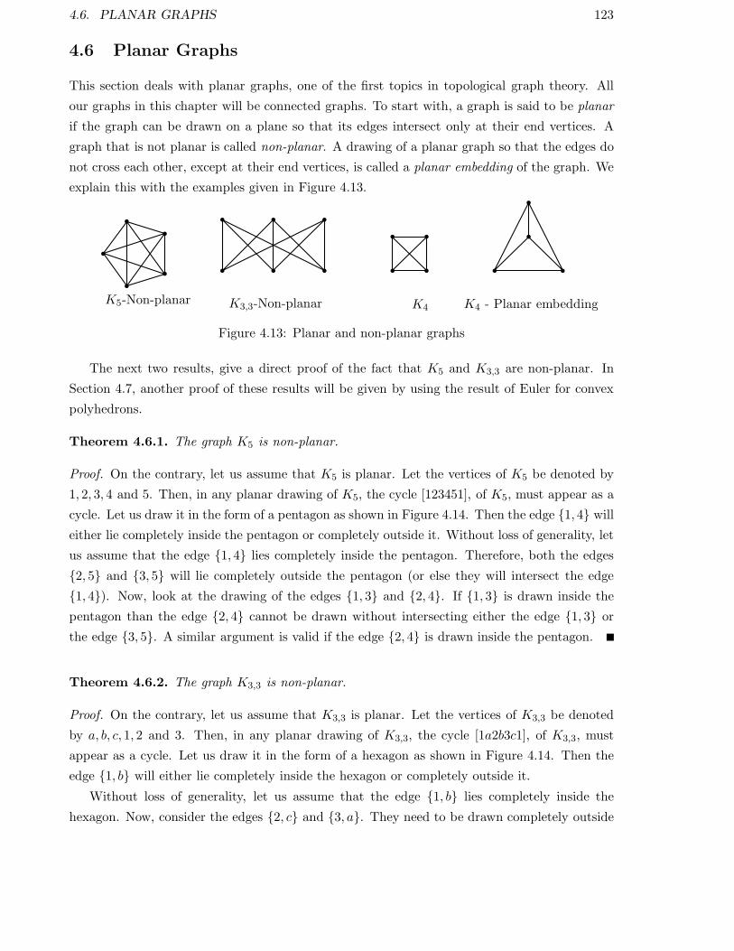
4.6. PLANAR GRAPHS 123
4.6 Planar Graphs
This section deals with planar graphs, one of the first topics in topological graph theory. All
our graphs in this chapter will be connected graphs. To start with, a graph is said to be planar
if the graph can be drawn on a plane so that its edges intersect only at their end vertices. A
graph that is not planar is called non-planar. A drawing of a planar graph so that the edges do
not cross each other, except at their end vertices, is called a planar embedding of the graph. We
explain this with the examples given in Figure 4.13.
K5-Non-planar K3,3-Non-planar K4 K4 - Planar embedding
Figure 4.13: Planar and non-planar graphs
The next two results, give a direct proof of the fact that K5 and K3,3 are non-planar. In
Section 4.7, another proof of these results will be given by using the result of Euler for convex
polyhedrons.
Theorem 4.6.1. The graph K5 is non-planar.
Proof. On the contrary, let us assume that K5 is planar. Let the vertices of K5 be denoted by
1, 2, 3, 4 and 5. Then, in any planar drawing of K5, the cycle [123451], of K5, must appear as a
cycle. Let us draw it in the form of a pentagon as shown in Figure 4.14. Then the edge 1, 4 will
either lie completely inside the pentagon or completely outside it. Without loss of generality, let
us assume that the edge 1, 4 lies completely inside the pentagon. Therefore, both the edges
2, 5 and 3, 5 will lie completely outside the pentagon (or else they will intersect the edge
1, 4). Now, look at the drawing of the edges 1, 3 and 2, 4. If 1, 3 is drawn inside the
pentagon than the edge 2, 4 cannot be drawn without intersecting either the edge 1, 3 or
the edge 3, 5. A similar argument is valid if the edge 2, 4 is drawn inside the pentagon.
Theorem 4.6.2. The graph K3,3 is non-planar.
Proof. On the contrary, let us assume that K3,3 is planar. Let the vertices of K3,3 be denoted
by a, b, c, 1, 2 and 3. Then, in any planar drawing of K3,3, the cycle [1a2b3c1], of K3,3, must
appear as a cycle. Let us draw it in the form of a hexagon as shown in Figure 4.14. Then the
edge 1, b will either lie completely inside the hexagon or completely outside it.
Without loss of generality, let us assume that the edge 1, b lies completely inside the
hexagon. Now, consider the edges 2, c and 3, a. They need to be drawn completely outside

124 CHAPTER 4. TOPICS IN CLASSICAL GRAPH THEORY
1
23
4
5K5-Non-planar
1
23
4
51
23
4
5
1 2 3
a b c
K3,3-Non-planar
1b
a2
c3
Figure 4.14: Non-planarity of the graphs K5 and K3,3
the hexagon (or else they will intersect the edge 1, b). Once 2, c is drawn outside the
hexagon then the edge 3, a cannot be drawn without intersecting either the edge 1, b or the
edge 2, c. A similar argument is valid if the edge 3, a is drawn outside the hexagon.
Thus, we have shown that the graphs K5 and K3,3 are non-planar. It can be easily observed
that if X is a graph that has K5 or K3,3 as its subgraph then X will also be non-planar. A
necessary and sufficient condition for a graph to be non-planar was given by Kuratowski. To
understand the statement of the theorem, we need to know the condition under which two graphs
are homeomorphic.
Let X = (V,E) be a graph. Let e = u, v be an edge of X and let z 6∈ V . Then, the
graph Y = (V ′, E′) is said to be obtained from the graph X = (V,E) by insertion of the vertex
z if V ′ = V ∪ z and E′ = (E \ e) ∪ u, z, z, v. That is, Y has been obtained from X
by dividing the edge e = u, v into two edges u, z and z, v, or equivalently, a vertex z of
degree 2 has been introduced on the edge e. This process of insertion of a new vertex of degree
2 is sometimes called subdivision of an edge. The inverse of this process is called edge merging.
A repeated application of edge subdivision leads to the following definition.
Definition 4.6.3. Let X and Y be two graphs. Then they are said to be homeomorphic if both
X and Y can be obtained from a graph, say Z, by inserting new vertices of degree 2 on the edges
of Z.
For example, all the paths are homeomorphic to each other and in particular to the graph
K2. Similarly, all the cyclic graphs are homeomorphic to the cycle C3, when one is interested
in the study of simple graphs. In general, one can say that all cyclic graphs are homeomorphic
to a graph X = (V,E), where V = v and E = e, e (i.e., a graph having exactly one vertex
and a loop). Also, note that if two graphs are isomorphic then they are also homeomorphic.
Figure 4.15 gives examples of homeomorphic graphs that are different from a path or a cycle.

4.6. PLANAR GRAPHS 125
Figure 4.15: Homeomorphic graphs
With this understanding, the theorem of Kuratowski states that “a simple connected graph
is planar if and only if it does not contain any subgraph that is homeomorphic to either K5 or
K3,3”. The proof of the theorem is out of the scope of these notes. The interested readers can
see the book “graph theory” by Harary [6] for a proof. We end this section with the following
observations which directly follow from Kuratowski theorem.
Observations:
1. Among all simple connected non-planar graphs
(a) the complete graph K5 has minimum number of vertices.
(b) the complete bipartite graph K3,3 has minimum number of edges.
2. If Y is a non-planar subgraph of a graph X then X is also non-planar.
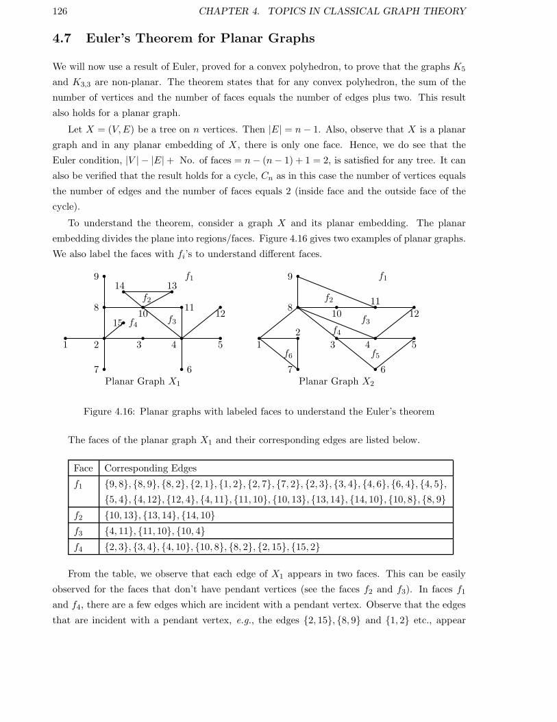
126 CHAPTER 4. TOPICS IN CLASSICAL GRAPH THEORY
4.7 Euler’s Theorem for Planar Graphs
We will now use a result of Euler, proved for a convex polyhedron, to prove that the graphs K5
and K3,3 are non-planar. The theorem states that for any convex polyhedron, the sum of the
number of vertices and the number of faces equals the number of edges plus two. This result
also holds for a planar graph.
Let X = (V,E) be a tree on n vertices. Then |E| = n− 1. Also, observe that X is a planar
graph and in any planar embedding of X, there is only one face. Hence, we do see that the
Euler condition, |V | − |E|+ No. of faces = n− (n− 1) + 1 = 2, is satisfied for any tree. It can
also be verified that the result holds for a cycle, Cn as in this case the number of vertices equals
the number of edges and the number of faces equals 2 (inside face and the outside face of the
cycle).
To understand the theorem, consider a graph X and its planar embedding. The planar
embedding divides the plane into regions/faces. Figure 4.16 gives two examples of planar graphs.
We also label the faces with fi’s to understand different faces.
15
3 4 51 2
6
8
9
1011
12
7
1314f1
f2
f3f4
Planar Graph X1
3 4 512
6
8
9
1011
12
7
f1
f2
f3f4
f5f6
Planar Graph X2
Figure 4.16: Planar graphs with labeled faces to understand the Euler’s theorem
The faces of the planar graph X1 and their corresponding edges are listed below.
Face Corresponding Edges
f1 9, 8, 8, 9, 8, 2, 2, 1, 1, 2, 2, 7, 7, 2, 2, 3, 3, 4, 4, 6, 6, 4, 4, 5,5, 4, 4, 12, 12, 4, 4, 11, 11, 10, 10, 13, 13, 14, 14, 10, 10, 8, 8, 9
f2 10, 13, 13, 14, 14, 10f3 4, 11, 11, 10, 10, 4f4 2, 3, 3, 4, 4, 10, 10, 8, 8, 2, 2, 15, 15, 2
From the table, we observe that each edge of X1 appears in two faces. This can be easily
observed for the faces that don’t have pendant vertices (see the faces f2 and f3). In faces f1
and f4, there are a few edges which are incident with a pendant vertex. Observe that the edges
that are incident with a pendant vertex, e.g., the edges 2, 15, 8, 9 and 1, 2 etc., appear

4.7. EULER’S THEOREM FOR PLANAR GRAPHS 127
twice when traversing a particular face. This observation leads to the proof of Euler’s theorem
for planar graphs which is the next result.
Theorem 4.7.1. Let X = (V,E) be a connected planar graph. Then the number of faces,
denoted Nf , in any planar embedding of X satisfies
|V | − |E|+Nf = 2.
Proof. We prove the result by induction on Nf , the number of faces of the graph. Let Nf = 1.
Then it can be easily observed that X cannot have a subgraph that is isomorphic to a cycle.
For if, X has a subgraph isomorphic to a cycle then in any planar embedding of X, Nf ≥ 2.
Therefore, X is a connected graph without cycle and hence X is a tree and this case has already
been verified in the second paragraph of this section.
So, let us assume that the result is true whenever a planar embedding results in Nf ≤ n.
Now, let X be a connected planar graph whose embedding results in Nf (X) = n + 1. Now,
choose an edge that is not a cut-edge, say e. Then X \ e is still a connected graph. Also, the
edge e is incident with two separate faces and hence it’s removal will combine the two faces and
thus X \ e has only n faces. Thus, by induction hypothesis,
|V (X \ e)| − |E(X \ e)|+Nf (X \ e) = 2.
This in turn implies that |V (X)| − |E(X)| +Nf (X) = 2 as |V (X \ e)| = |V (X)|, |E(X \ e)| =|E(X)| − 1 and Nf (X \ e) = Nf (X) + 1.
Thus, by the principle of mathematical induction, the result holds.
Theorem 4.7.1 implies that the number of faces of a planar graph is independent of the
embedding as it is just a function of the number of vertices and the number of edges of a graph,
which are graph invariants. This observation leads to the next result and hence the proof is
omitted.
Corollary 4.7.2. Let X be a connected planar graph. Then Nf (X), the number of faces of X,
is independent of the planar embedding.
Theorem 4.7.1 can be used to obtain quite a few inequalities involving the number of vertices
and the number of edges of a planar graph. We state them next and use them to prove that the
graphs K5 and K3,3 are non-planar.
Corollary 4.7.3. Let X be a connected planar graph having n vertices and m edges. If n ≥ 3,
then m ≤ 3n− 6.
Proof. Without loss of generality, let us assume that X is a simple connected planar graph with
n ≥ 3. Then a face of X can be enclosed with at least 3 edges. As each edge is incident with
exactly two faces, one has 2m = 2|E| ≥ 3Nf . Thus, using Euler’s theorem, we have
2 = |V | − |E|+Nf = n−m+Nf ≤ n−m+2
3m

128 CHAPTER 4. TOPICS IN CLASSICAL GRAPH THEORY
and hence the required result follows.
Corollary 4.7.4. The complete graph K5 is non-planar.
Proof. Suppose there exists a planar embedding of K5. Then the Corollary 4.7.3 implies that
10 = |E(K5)| ≤ 3|V (K5)| − 6 = 3× 5− 6 = 9,
a contradiction. Thus, the required result follows.
An idea similar to the idea used in the proof of Corollary 4.7.3 gives another prove of the
non-planarity of K3,3.
Corollary 4.7.5. The complete bipartite graph K3,3 is non-planar.
Proof. Suppose there exists a planar embedding of K3,3. Note that the condition that K3,3 is
bipartite (each cycle of K3,3 consists of at least 4 edges), in each planar embedding of K3,3, each
face of of the embedding will be enclosed with at least 4 edges.
Then, as in the proof of Corollary 4.7.2, one has 2m = 2|E| ≥ 4Nf . Thus, using Euler’s
theorem, we have
2 = |V | − |E|+Nf ≤ n−m+m
2≤ 6− 9 +
9
2=
3
2,
a contradiction and hence the required result follows.
Corollary 4.7.6. Let X be a simple connected planar graph. Then X has a vertex of degree
less than or equal to 5.
Proof. Let δ = mindeg(v) : v ∈ V (X). Then we need to show that δ ≤ 5.
If |V (X)| ≤ 2, then there is nothing to prove. So, let us assume that |V (X)| ≥ 3. Thus,
by definition 2|E| = ∑
v∈V (X)
deg(v) ≥ δ|V (X)|. Now, using Corollary 4.7.3, one has δ|V (X)| ≤
2(3|V (X)|− 6
)or equivalently, (6− δ)|V (X)| ≥ 12 and hence δ ≤ 5. Thus, one has the required
result.
This result is used in the proof of the five color theorem. This result is out of the scope of
this book. The interested readers are advised to see the book “Graph Theory” by Harary [6].

4.8. STEREOGRAPHIC PROJECTION 129
4.8 Stereographic Projection
Consider the two graphs in Figure 4.16. The faces have been denoted with fi, for some positive
integer i. Note that in the embedding of both the graphs, there is a face, denoted f1, which
seems to be an infinite face, whereas the other faces seem to be enclosed by the edges of the
graphs. It turns out that the face f1, which seems to form an infinite face, can be made into
a closed face by embedding the graph into a sphere and then projecting it back on to a plane
after rotating the sphere in such a way that a point of the face f1 touches the plane. This idea
will be clear at the end of this section. This projection is called the stereographic projection. An
example of the same has been shown in Figure 4.17.
Np
Figure 4.17: Stereographic projection
The stereographic projection consists of the following:
• place a sphere on the plane and let Sp be the point on the sphere that touches the plane.
The point Sp is called the south pole.
• Now, draw the line passing through the point Sp and the center of the sphere. This line
intersects the sphere at a point, say Np. The point Np is called the north pole of the
sphere. See Figure 4.17 for the north pole.
• Now, given any point x on the sphere, draw a straight line that passes through Np and
x. This line will intersect the plane at a unique point, say y. Then the stereographic
projection of the point x is defined to be the point y on the plane.
It can be easily observed that the stereographic projection, defined above, has an inverse
map, which maps any point on the plane to a point on the sphere. To do this, let y1 be a point
on the plane. Join the point y1 with Np, the north pole. Then this line will intersect the sphere
at a unique point. This point will be the inverse image of the point y1. Also, the image of

130 CHAPTER 4. TOPICS IN CLASSICAL GRAPH THEORY
the point Np, the north pole, under the stereographic projection is the point at infinity in the
extended plane (i.e., R2 ∪ ∞).Before proceeding with the result that states that every face of planar embedding of a planar
graph X can be made into an infinite face and/or bounded face, we observe that using the
stereographic projection, a planar embedding and embedding on a sphere are one and the same.
Theorem 4.8.1. Let v be a vertex of a connected planar graph X. Then X can be embedded in
the plane in such a way that v is on the exterior face of the embedding.
Proof. Let X be a planar embedding of X. Use the stereographic projection to project this
embedding on the sphere. Let this embedding on the sphere be called Z. It is clear that this
embedding exists, as explained in previous paragraphs. Now let f be the face that has v as one
of its vertices. Take a point z in f and fix it. Now, place the sphere, on a plane, in such a way
that the point z (on the sphere) acts as the north pole. Then the projection of the embedding
Z with the point z as the north pole, gives a planar embedding of X with the required property.