
Discrete Mathematics - Mr. Coach Lowe / FrontPage
92
699 Discrete Mathematics As the use of cellular telephones, modems, pagers, and fax machines has grown in recent years, the increasing demand for unique telephone numbers has necessitated the creation of new area codes in many areas of the United States. Counting the number of possible telephone numbers in a given area code is a combinatorial problem, and such problems are solved using the techniques of discrete mathematics. See page 707 for more on the subject of telephone area codes. 9.1 Basic Combinatorics 9.2 The Binomial Theorem 9.3 Probability 9.4 Sequences 9.5 Series 9.6 Mathematical Induction 9.7 Statistics and Data (Graphical) 9.8 Statistics and Data (Algebraic) CHAPTER 9
-
Upload
khangminh22 -
Category
Documents
-
view
1 -
download
0
Transcript of Discrete Mathematics - Mr. Coach Lowe / FrontPage

699
Discrete Mathematics
As the use of cellular telephones, modems, pagers, andfax machines has grown in recent years, the increasingdemand for unique telephone numbers has necessitatedthe creation of new area codes in many areas of theUnited States. Counting the number of possible telephonenumbers in a given area code is a combinatorial problem,and such problems are solved using the techniques of discrete mathematics. See page 707 for more on the subject of telephone area codes.
9.1 Basic Combinatorics
9.2 The BinomialTheorem
9.3 Probability
9.4 Sequences
9.5 Series
9.6 MathematicalInduction
9.7 Statistics and Data(Graphical)
9.8 Statistics and Data(Algebraic)
C H A P T E R 9
5144_Demana_Ch09pp699-790 1/13/06 3:05 PM Page 699

Chapter 9 OverviewThe branches of mathematics known broadly as algebra, analysis, and geometrycome together so beautifully in calculus that it has been difficult over the years tosqueeze other mathematics into the curriculum. Consequently, many worthwhile top-ics like probability and statistics, combinatorics, graph theory, and numerical analy-sis that could easily be introduced in high school are (for many students) either firstseen in college electives or else never seen at all. This situation is gradually chang-ing as the applications of noncalculus mathematics become increasingly more impor-tant in the modern, computerized, data-driven workplace. Therefore, besides intro-ducing important topics like sequences and series and the Binomial Theorem, thischapter will touch on some other discrete topics that might prove useful to you in thenear future.
700 CHAPTER 9 Discrete Mathematics
9.1Basic CombinatoricsWhat you’ll learn about■ Discrete Versus Continuous
■ The Importance of Counting
■ The Multiplication Principleof Counting
■ Permutations
■ Combinations
■ Subsets of an n-Set
. . . and whyCounting large sets is easy ifyou know the correct formula.
Discrete Versus ContinuousA point has no length and no width, and yet intervals on the real line—which are madeup of these dimensionless points—have length! This little mystery illustrates the distinction between continuous and discrete mathematics. Any interval (a, b) containsa of real numbers, which is why you can zoom in on an interval foreverand there will still be an interval there. Calculus concepts like limits and continuitydepend on the mathematics of the continuum. In discrete mathematics, we are con-cerned with properties of numbers and algebraic systems that do not depend on thatkind of analysis. Many of them are related to the first kind of mathematics that most ofus ever did, namely counting. Counting is what we will do for the rest of this section.
The Importance of CountingWe begin with a relatively simple counting problem.
continuum
BIBLIOGRAPHYFor students: Images of Infinity, GeraldJenkins (Ed.), Leapfrog Group, 1995.For teachers: Discrete Mathematics inthe Schools, Joseph G. Rosenstein,Deborah S. Franzblau, Fred S. Roberts(Eds.), NCTM and AMS, 1998.
Discrete Mathematics ThroughApplications, Nancy Crisley et al., W. H.Freeman, 1994.
VideosDiscrete Mathematics: Cracking theCode, COMAP Video
EXAMPLE 1 Arranging Three Objects in OrderIn how many different ways can three distinguishable objects be arranged in order?
SOLUTION It is not difficult to list all the possibilities. If we call the objects A, B,and C, the different orderings are: ABC, ACB, BAC, BCA, CAB, and CBA. A good wayto visualize the six choices is with a tree diagram, as in Figure 9.1. Notice that we havethree choices for the first letter. Then, branching off each of those three choices are twochoices for the second letter. Finally, branching off each of the 3 � 2 � 6 branchesformed so far is one choice for the third letter. By beginning at the “root” of the tree, wecan proceed to the right along any of the 3 � 2 � 1 � 6 branches and get a differentordering each time. We conclude that there are six ways to arrange three distinguishableobjects in order. Now try Exercise 3.FIGURE 9.1 A tree diagram for ordering
the letters ABC. (Example 1)
A
C
B
A
A
A
A
C
B
C
B
C
B
C
B
5144_Demana_Ch09pp699-790 1/13/06 3:05 PM Page 700

SECTION 9.1 Basic Combinatorics 701
Scientific studies will usually manipulate one or more variables and
observe the effect of that manipulation on one or more variables. The keyto understanding the significance of the effect is to know what is likely to occur bychance alone, and that often depends on counting. For example, Exploration 1shows a real-world application of Example 1.
responseexplanatory
OBJECTIVEStudents will be able to use the multiplica-tion principle of counting, permutations, orcombinations to count the number of waysthat a task can be done.
MOTIVATEAsk students to find the number of possibleways one can choose two marbles from abag containing three marbles: (1) if theorder is important (6), and (2) if the order isnot important (3).
LESSON GUIDEDay 1: Discrete Versus Continuous; TheImportance of Counting; The MultiplicationPrinciple of Counting; PermutationsDay 2: Combinations; Subsets of an n-set
The Multiplication Principle of CountingYou would not want to draw the tree diagram for ordering five objects (ABCDE), butyou should be able to see in your mind that it would have 5 � 4 � 3 � 2 � 1 � 120branches. A tree diagram is a geometric visualization of a fundamental counting prin-ciple known as the Multiplication Principle.
EXPLORATION 1 Questionable Product Claims
A salesman for a copying machine company is trying to convince a client tobuy his $2000 machine instead of his competitor’s $5000 machine. To makehis point, he lines up an original document, a copy made by his machine,and a copy made by the more expensive machine on a table and asks 60office workers to identify which is which. To everyone’s surprise, not a sin-gle worker identifies all three correctly. The salesman states triumphantlythat this proves that all three documents look the same to the naked eye andthat therefore the client should buy his company’s less expensive machine.
What do you think?
1. Each worker is essentially being asked to put the three documents in thecorrect order. How many ways can the three documents be ordered? 6
2. Suppose all three documents really do look alike. What fraction of theworkers would you expect to put them into the correct order by chancealone? 1/6
3. If zero people out of 60 put the documents in the correct order, should weconclude that “all three documents look the same to the naked eye”? No
4. Can you suggest a more likely conclusion that we might draw from theresults of the salesman’s experiment? It is likely that the salesman rigged the test
EXPLORATION EXTENSIONSA car manufacturing company asked 1000people to view their latest two-door coupeavailable in four colors (Alabaster White,Black, Cherry Red, and Dusk Blue). Theviewers were asked to list their color prefer-ences in order from favorite. How manyways could the colors be ordered? (24)Of the 1000 viewers, how many would youexpect to choose the preference orderAlabaster White, Black, Cherry Red, andDusk Blue? (41 2/3 � 42 people assumingall preferences are equally likely to bechosen.)
TEACHING NOTEIf time is limited for this chapter, the fol-lowing groups of topics can be coveredindependently:1. 9.1, 9.2, 9.32. 9.1, 9.3 (with omission of Binomial
Distributions)3. 9.4, 9.54. 9.6, 9.7
Multiplication Principle of Counting
If a procedure P has a sequence of stages S1, S2, . . . , Sn and if
S1 can occur in r1 ways,
S2 can occur in r2 ways,...
Sn can occur in rn ways,
then the number of ways that the procedure P can occur is the product
r1r2 � � � rn.
5144_Demana_Ch09pp699-790 1/13/06 3:05 PM Page 701

702 CHAPTER 9 Discrete Mathematics
PermutationsOne important application of the Multiplication Principle of Counting is to count thenumber of ways that a set of n objects (called an n-set) can be arranged in order. Eachsuch ordering is called a permutation of the set. Example 1 showed that there are3! � 6 permutations of a 3-set. In fact, if you understood the tree diagram, you canprobably guess how many permutations there are of an n-set.
It is important to be mindful of how the choices at each stage are affected by the choicesat preceding stages. For example, when choosing an order for the letters ABC we have3 choices for the first letter, but only 2 choices for the second and 1 for the third.
EXAMPLE 2 Using the Multiplication PrincipleThe Tennessee license plate shown here consists of three letters of the alphabet fol-lowed by three numerical digits (0 through 9). Find the number of different licenseplates that could be formed
(a) if there is no restriction on the letters or digits that can be used;
(b) if no letter or digit can be repeated.
SOLUTION Consider each license plate as having six blanks to be filled in: threeletters followed by three numerical digits.
(a) If there are no restrictions on letters or digits, then we can fill in the first blank 26 ways, the second blank 26 ways, the third blank 26 ways, the fourth blank 10 ways, the fifth blank 10 ways, and the sixth blank 10 ways. By the MultiplicationPrinciple, we can fill in all six blanks in 26 � 26 � 26 � 10 � 10 � 10 �17,576,000 ways. There are 17,576,000 possible license plates with no restric-tions on letters or digits.
(b) If no letter or digit can be repeated, then we can fill in the first blank 26 ways, thesecond blank 25 ways, the third blank 24 ways, the fourth blank 10 ways, the fifthblank 9 ways, and the sixth blank 8 ways. By the Multiplication Principle, we canfill in all six blanks in 26 � 25 � 24 � 10 � 9 � 8 � 11,232,000 ways. Thereare 11,232,000 possible license plates with no letters or digits repeated.
Now try Exercise 5.
TEACHER’S NOTEEncourage students to ask the followingquestions prior to actually doing any count-ing. (1) What is the process that is beingcompleted? Does the order matter (either interms of completing the problem correctlyor simplifying calculations)? (2) What is thefirst stage? How many ways can it be com-pleted? (3) What is the second stage? Howmany ways can it be completed? And so on.
LICENSE PLATE RESTRICTIONS
Although prohibiting repeated lettersand digits as in Example 2 would makeno practical sense (why rule out morethan 6 million possible plates for no goodreason?), states do impose some restric-tions on license plates. They rule out cer-tain letter progressions that could beconsidered obscene or offensive.
Permutations of an n-set
There are n! permutations of an n-set.
FACTORIALS
If n is a positive integer, the symbol n! (read “n factorial”) represents the prod-uct n(n � 1)(n � 2)(n � 3) � � � 2 • 1. Wealso define 0! � 1.
EXAMPLE 3 Distinguishable PermutationsCount the number of different 9-letter “words” (don’t worry about whether they’re inthe dictionary) that can be formed using the letters in each word.
(a) DRAGONFLY (b) BUTTERFLY (c) BUMBLEBEE
Usually the elements of a set are distinguishable from one another, but we can adjustour counting when they are not, as we see in Example 3.
continued
5144_Demana_Ch09pp699-790 1/13/06 3:06 PM Page 702

SECTION 9.1 Basic Combinatorics 703
In many counting problems, we are interested in using n objects to fill r blanks inorder, where r � n. These are called The procedure for counting them is the same; only this time we run out of blanksbefore we run out of objects.
The first blank can be filled in n ways, the second in n � 1 ways, and so on until we cometo the rth blank, which can be filled in n � �r � 1� ways. By the Multiplication Principle,we can fill in all r blanks in n�n � 1��n � 2� � � � �n � r � 1� ways. This expression canbe written in a more compact (but less easily computed) way as n!��n � r�!.
permutations of n objects taken r at a time.
SOLUTION
(a) Each permutation of the 9 letters forms a different word. There are 9! � 362,880such permutations.
(b) There are also 9! permutations of these letters, but a simple permutation of thetwo T’s does not result in a new word. We correct for the overcount by dividing
by 2!. There are 92!! � 181,440 distinguishable permutations of the letters in
BUTTERFLY.
(c) Again there are 9! permutations, but the three B’s are indistinguishable, as are the
three E’s, so we divide by 3! twice to correct for the overcount. There are 39!3!!
�
10,080 distinguishable permutations of the letters in BUMBLEBEE.
Now try Exercise 9.
Distinguishable Permutations
There are n! distinguishable permutations of an n-set containing n distinguishableobjects.
If an n-set contains n1 objects of a first kind, n2 objects of a second kind, and soon, with n1 � n2 �� � �� nk � n, then the number of distinguishable permutationsof the n-set is
n1!n2!n3
n!!� � � nk!.
Permutation Counting Formula
The number of permutations of n objects taken r at a time is denoted nPr and isgiven by
nPr � �n �
n!r�!
for 0 r n.
If r � n, then nPr � 0.
Notice that nPn � n!��n � n�! � n!�0! � n!�1 � n!, which we have already seen is thenumber of permutations of a complete set of n objects. This is why we define 0! � 1.
PERMUTATIONS ON A CALCULATOR
Most modern calculators have an nPr
selection built in. They also computefactorials, but remember that factorialsget very large. If you want to count thenumber of permutations of 90 objectstaken 5 at a time, be sure to use the nPr
function. The expression 90!/85! is likelyto lead to an overflow error.
5144_Demana_Ch09pp699-790 1/13/06 3:06 PM Page 703

704 CHAPTER 9 Discrete Mathematics
NOTES ON EXAMPLEExample 4 shows some paper-and-pencilmethods for calculating permutations. It isimportant that students have the algebraicskills to perform these operations since thenumbers in some counting problems mayexceed the capacity of a calculator.
CombinationsWhen we count permutations of n objects taken r at a time, we consider different order-ings of the same r selected objects as being different permutations. In many applicationswe are only interested in the ways to select the r objects, regardless of the order inwhich we arrange them. These unordered selections are called objects taken r at a time.
combinations of n
EXAMPLE 4 Counting PermutationsEvaluate each expression without a calculator.
(a) 6P4 (b) 11P3 (c) nP3
SOLUTION
(a) By the formula, 6P4 � 6!��6 � 4�! � 6!�2! � �6 • 5 • 4 • 3 • 2!��2! � 6 • 5 • 4 • 3 �360.
(b) Although you could use the formula again, you might prefer to apply theMultiplication Principle directly. We have 11 objects and 3 blanks to fill:
11P3 � 11 • 10 • 9 � 990.
(c) This time it is definitely easier to use the Multiplication Principle. We have nobjects and 3 blanks to fill; so assuming n � 3,
nP3 � n�n � 1��n � 2�.
Now try Exercise 15.
Combination Counting Formula
The number of combinations of n objects taken r at a time is denoted nCr and isgiven by
nCr � r!�n
n�
!r�!
for 0 r n.
If r � n, then nCr � 0.
EXAMPLE 5 Applying PermutationsSixteen actors answer a casting call to try out for roles as dwarfs in a production ofSnow White and the Seven Dwarfs. In how many different ways can the director castthe seven roles?
SOLUTION The 7 different roles can be thought of as 7 blanks to be filled, and we have 16 actors with which to fill them. The director can cast the roles in
16P7 � 57,657,600 ways. Now try Exercise 12.
5144_Demana_Ch09pp699-790 1/13/06 3:06 PM Page 704

SECTION 9.1 Basic Combinatorics 705
We can verify the nCr formula with the Multiplication Principle. Since every permuta-tion can be thought of as an unordered selection of r objects followed by a particularordering of the objects selected, the Multiplication Principle gives nPr � nCr • r!.
Therefore
nCr � nrP!r �
r1! •
�n �
n!r�!
� r!�n
n�
!r�!
.
EXAMPLE 6 Distinguishing Combinationsfrom Permutations
In each of the following scenarios, tell whether permutations (ordered) or combina-tions (unordered) are being described.
(a) A president, vice-president, and secretary are chosen from a 25-member gardenclub.
(b) A cook chooses 5 potatoes from a bag of 12 potatoes to make a potato salad.
(c) A teacher makes a seating chart for 22 students in a classroom with 30 desks.
SOLUTION
(a) Permutations. Order matters because it matters who gets which office.
(b) Combinations. The salad is the same no matter what order the potatoes are chosen.
(c) Permutations. A different ordering of students in the same seats results in a dif-ferent seating chart.
Notice that once you know what is being counted, getting the correct number is easywith a calculator. The number of possible choices in the scenarios above are: (a) 25P3 �13,800, (b) 12C5 � 792, and (c) 30P22 � 6.5787 � 1027.
Now try Exercise 19.
EXAMPLE 7 Counting CombinationsIn the Miss America pageant, 51 contestants must be narrowed down to 10 finalistswho will compete on national television. In how many possible ways can the tenfinalists be selected?
SOLUTION Notice that the order of the finalists does not matter at this phase; allthat matters is which women are selected. So we count combinations rather than permutations.
51C10 � 10
5!14!1!
� 12,777,711,870.
The 10 finalists can be chosen in 12,777,711,870 ways.
Now try Exercise 27.
A WORD ON NOTATION
Some textbooks use P�n, r� instead of nPr
and C(n, r) instead of nCr. Much more
common is the notation ( ) for nCr. Bothn
r
COMBINATIONS ON A CALCULATOR
Most modern calculators have an nCrselection built in. As with permutations,it is better to use the nCr function than
to use the formula r!(n
n�
!r)!
, as the
individual factorials can get too largefor the calculator.
( ) and nCr are often read “n choose r.”n
r
5144_Demana_Ch09pp699-790 1/13/06 3:06 PM Page 705
706 CHAPTER 9 Discrete Mathematics
ALERTSome students find counting problemsvery challenging. They often want toapply a formula blindly rather than to gothrough a thinking process. In particular,students frequently forget to pay attentionto whether or not the order is important ina particular problem.
The solution to Example 9b suggests a general rule that will be our last counting for-mula of the section.
Formula for Counting Subsets of an n-Set
There are 2n subsets of a set with n objects (including the empty set and the entire set).
EXAMPLE 8 Picking Lottery NumbersThe Georgia Lotto requires winners to pick 6 integers between 1 and 46. The order inwhich you select them does not matter; indeed, the lottery tickets are always printedwith the numbers in ascending order. How many different lottery tickets are possible?
SOLUTION There are 46C6 � 9,366,819 possible lottery tickets of this type.(That’s more than enough different tickets for every person in the state of Georgia!)
Now try Exercise 29.
Subsets of an n-SetAs a final application of the counting principle, consider the pizza topping problem.
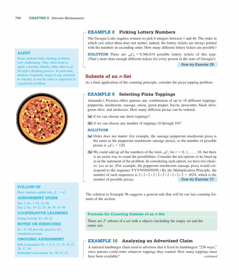
EXAMPLE 9 Selecting Pizza ToppingsArmando’s Pizzeria offers patrons any combination of up to 10 different toppings:pepperoni, mushroom, sausage, onion, green pepper, bacon, prosciutto, black olive,green olive, and anchovies. How many different pizzas can be ordered
(a) if we can choose any three toppings?
(b) if we can choose any number of toppings (0 through 10)?
SOLUTION
(a) Order does not matter (for example, the sausage-pepperoni-mushroom pizza isthe same as the pepperoni-mushroom-sausage pizza), so the number of possiblepizzas is 10C3 � 120.
(b) We could add up all the numbers of the form 10Cr for r � 0, 1, . . . , 10, but thereis an easier way to count the possibilities. Consider the ten options to be lined upas in the statement of the problem. In considering each option, we have two choic-es: yes or no. (For example, the pepperoni-mushroom-sausage pizza would cor-respond to the sequence YYYNNNNNNN.) By the Multiplication Principle, thenumber of such sequences is 2 • 2 • 2 • 2 • 2 • 2 • 2 • 2 • 2 • 2 � 1024, which is thenumber of possible pizzas. Now try Exercise 37.
FOLLOW-UPHave students explain why nPn � n!.
ASSIGNMENT GUIDEDay 1: Ex. 1–12, 23–26Day 2: Ex. 19–22, 29, 36–39, 43–48
COOPERATIVE LEARNINGGroup Activity: Ex. 49, 52
NOTES ON EXERCISESEx. 43–48 provide practice for standardized tests.
ONGOING ASSESSMENTSelf-Assessment: Ex. 3, 5, 9, 12, 15, 19, 27,29, 37, 39Embedded Assessment: Ex. 50, 51, 53
EXAMPLE 10 Analyzing an Advertised ClaimA national hamburger chain used to advertise that it fixed its hamburgers “256 ways,”since patrons could order whatever toppings they wanted. How many toppings musthave been available? continued
5144_Demana_Ch09pp699-790 1/13/06 3:06 PM Page 706
SECTION 9.1 Basic Combinatorics 707
SOLUTION We need to solve the equation 2n � 256 for n. We could solve this eas-ily enough by trial and error, but we will solve it with logarithms just to keep themethod fresh in our minds.
2n � 256
log 2n � log 256
n log 2 � log 256
n � lolgog
2526
n � 8
There must have been 8 toppings from which to choose.
Now try Exercise 39.
WHY ARE THERE NOT 1000 POSSIBLE
AREA CODES?
While there are 1000 three-digit numbersbetween 000 and 999, not all of them areavailable for use as area codes. For exam-ple, area codes cannot begin with 0 or 1,and numbers of the form abb have beenreserved for other purposes.
CHAPTER OPENER PROBLEM (from page 699)
PROBLEM: There are 680 three-digit numbers that are available for use as areacodes in North America. As of April 2002, 305 of them were actually being used(Source: www.nanpa.com). How many additional three-digit area codes are avail-able for use? Within a given area code, how many unique telephone numbers aretheoretically possible?
SOLUTION: There are 680 � 305 � 375 additional area codes available.Within a given area code, each telephone number has seven digits chosen from theten digits 0 through 9. Since each digit can theoretically be any of 10 numbers,there are
10 • 10 • 10 • 10 • 10 • 10 • 10 � 107 � 10,000,000
different telephone numbers possible within a given area code.
Putting these two results together, we see that the unused area codes in April 2002represented an additional 3.75 billion possible telephone numbers!
QUICK REVIEW 9.1In Exercises 1–10, give the number of objects described. In somecases you might have to do a little research or ask a friend.
1. The number of cards in a standard deck 52
2. The number of cards of each suit in a standard deck 13
3. The number of faces on a cubical die 6
4. The number of possible totals when two dice are rolled 11
5. The number of vertices of a decagon 10
6. The number of musicians in a string quartet 4
7. The number of players on a soccer team 11
8. The number of prime numbers between 1 and 10, inclusive 4
9. The number of squares on a chessboard 64
10. The number of cards in a contract bridge hand 13
5144_Demana_Ch09pp699-790 1/13/06 3:06 PM Page 707

708 CHAPTER 9 Discrete Mathematics
20. 7 digits are selected (without repetition) to form a telephone number. permutations
21. 4 students are selected from the senior class to form a committeeto advise the cafeteria director about food. combinations
22. 4 actors are chosen to play the Beatles in a film biography.
23. License Plates How many different license plates begin withtwo digits, followed by two letters and then three digits if no let-ters or digits are repeated? 19,656,000
24. License Plates How many different license plates consist offive symbols, either digits or letters? 60,466,176
25. Tumbling Dice Suppose that two dice, one red and one green,are rolled. How many different outcomes are possible for the pairof dice? 36
26. Coin Toss How many different sequences of heads and tails arethere if a coin is tossed 10 times? 1024
27. Forming Committees A 3-woman committee is to be electedfrom a 25-member sorority. How many different committees canbe elected? 2300
28. Straight Poker In the original version of poker known as“straight” poker, a five-card hand is dealt from a standarddeck of 52. How many different straight poker hands arepossible? 2,598,960
29. Buying Discs Juan has money to buy only three of the 48 com-pact discs available. How many different sets of discs can he pur-chase? 17,296
30. Coin Toss A coin is tossed 20 times and the heads and tailssequence is recorded. From among all the possible sequences ofheads and tails, how many have exactly seven heads? 77,520
31. Drawing Cards How many different 13-card hands include theace and king of spades? 37,353,738,800
32. Job Interviews The head of the personnel department inter-views eight people for three identical openings. How many differ-ent groups of three can be employed? 56
33. Scholarship Nominations Six seniors at Rydell High Schoolmeet the qualifications for a competitive honor scholarship at amajor university. The university allows the school to nominate upto three candidates, and the school always nominates at least one.How many different choices could the nominating committeemake? 41
34. Pu-pu Platters A Chinese restaurantwill make a Pu-pu platter “to order”containing any one, two, or three selec-tions from its appetizer menu. If themenu offers five different appetizers,how many different platters could bemade? 25
SECTION 9.1 EXERCISES
In Exercises 1–4, count the number of ways that each procedure canbe done.
1. Line up three people for a photograph. 6
2. Prioritize four pending jobs from most to least important. 24
3. Arrange five books from left to right on a bookshelf. 120
4. Award ribbons for 1st place to 5th place to the top five dogs in adog show. 120
5. Homecoming King and Queen There are four candidates forhomecoming queen and three candidates for king. How manyking-queen pairs are possible? 12
6. Possible Routes There are three roads from town A to town B and four roads from town B to town C. How many differ-ent routes are there from A to C by way of B? 12
7. Permuting Letters How many 9-letter “words” (not necessarily in any dictionary) can be formed from the lettersof the word LOGARITHM? (Curiously, one such arrange-ment spells another word related to mathematics. Can youname it?) 362,880 (ALGORITHM)
8. Three-Letter Crossword Entries Excluding J, Q, X, and Z,how many 3-letter crossword puzzle entries can be formed thatcontain no repeated letters? (It has been conjectured that all ofthem have appeared in puzzles over the years, sometimes withpainfully contrived definitions.) 9240
9. Permuting Letters How many distinguishable 11-letter“words” can be formed using the letters in MISSISSIPPI? 34,650
10. Permuting Letters How many distinguishable 11-letter“words” can be formed using the letters in CHATTANOOGA? 1,663,200
11. Electing Officers The 13 members of the East BrainerdGarden Club are electing a President, Vice-President, andSecretary from among their members. How many different wayscan this be done? 1716
12. City Government From among 12 projects under considera-tion, the mayor must put together a prioritized (that is, ordered)list of 6 projects to submit to the city council for funding. Howmany such lists can be formed? 665,280
In Exercises 13–18, evaluate each expression without a calculator. Thencheck with your calculator to see if your answer is correct.
13. 4! 24 14. �3!��0!� 6
15. 6P2 30 16. 9P2 72
17. 10C7 120 18. 10C3 120
In Exercises 19–22, tell whether permutations (ordered) or combinations (unordered) are being described.
19. 13 cards are selected from a deck of 52 to form a bridge hand.combinations
5144_Demana_Ch09pp699-790 1/13/06 3:06 PM Page 708

35. Yahtzee In the game of Yahtzee, five dice are tossed simultane-ously. How many outcomes can be distinguished if all the dice aredifferent colors? 7776
36. Indiana Jones and the Final Exam Professor Indiana Jonesgives his class 20 study questions, from which he will select 8 tobe answered on the final exam. How many ways can he select thequestions? 125,970
37. Salad Bar Mary’s lunch always consists of a full plate of saladfrom Ernestine’s salad bar. She always takes equal amounts ofeach salad she chooses, but she likes to vary her selections. If shecan choose from among 9 different salads, how many essentiallydifferent lunches can she create? 511
38. Buying a New Car A new car customer has to choose fromamong 3 models, each of which comes in 4 exterior colors, 3 inte-rior colors, and with any combination of up to 6 optional acces-sories. How many essentially different ways can the customerorder the car? 2304
39. Pizza Possibilities Luigi sells one size of pizza, but he claimsthat his selection of toppings allows for “more than 4000 differentchoices.” What is the smallest number of toppings Luigi couldoffer? 12
40. Proper Subsets A subset of set A is called proper if it is nei-ther the empty set nor the entire set A. How many proper subsetsdoes an n-set have? 2n � 2
41. True-False Tests How many different answer keys are possiblefor a 10-question True-False test? 1024
42. Multiple-Choice Tests How many different answer keys arepossible for a 10-question multiple-choice test in which eachquestion leads to choice a, b, c, d, or e? 9,765,625
Standardized Test Questions43. True or False If a and b are positive integers such that
a � b � n, then ( ) � ( ). Justify your answer.
44. True or False If a, b, and n are integers such that
a � b � n, then ( ) � ( ). Justify your answer.
You may use a graphing calculator when evaluating Exercises 45–48.
45. Multiple Choice Lunch at the Gritsy Palace consists of anentrée, two vegetables, and a dessert. If there are four entrées, sixvegetables, and six desserts from which to choose, how manyessentially different lunches are possible? D
(A) 16
(B) 25
(C) 144
(D) 360
(E) 720
nb
na
nb
na
46. Multiple Choice How many different ways can the judgeschoose 5th to 1st places from ten Miss America finalists? D
(A) 50
(B) 120
(C) 252
(D) 30,240
(E) 3,628,800
47. Multiple Choice Assuming r and n are positive integers withr � n, which of the following numbers does not equal 1? B
(A) (n � n)!
(B) nPn
(C) nCn
(D) ( )(E) ( ) ( )
48. Multiple Choice An organization is electing 3 new board mem-bers by approval voting. Members are given ballots with the namesof 5 candidates and are allowed to check off the names of all candi-dates whom they would approve (which could be none, or even allfive). The three candidates with the most checks overall are elected.In how many different ways can a member fill out the ballot? C
(A) 10
(B) 20
(C) 32
(D) 125
(E) 243
Explorations49. Group Activity For each of the following numbers, make up
a counting problem that has the number as its answer.
(a) 52C3
(b) 12C3
(c) 25P11
(d) 25
(e) 3 • 210
50. Writing to Learn You have a fresh carton containing onedozen eggs and you need to choose two for breakfast. Givea counting argument based on this scenario to explain why
12C2 � 12C10.
51. Factorial Riddle The number 50! ends in a string of consecutive 0’s.
(a) How many 0’s are in the string? 12
(b) How do you know?
nn � r
nr
nn
SECTION 9.1 Basic Combinatorics 709
5144_Demana_Ch09pp699-790 1/13/06 3:06 PM Page 709
52. Group Activity Diagonals of a Regular Polygon InExploration 1 of Section 1.6, you reasoned from data points andquadratic regression that the number of diagonals of a regularpolygon with n vertices was �n2 � 3n��2.
(a) Explain why the number of segments connecting all pairs ofvertices is nC2.
(b) Use the result from part (a) to prove that the number of diago-nals is �n2 � 3n��2.
Extending the Ideas53. Writing to Learn Suppose that a chain letter (illegal if money
is involved) is sent to five people the first week of the year. Eachof these five people sends a copy of the letter to five more peopleduring the second week of the year. Assume that everyone whoreceives a letter participates. Explain how you know with certain-ty that someone will receive a second copy of this letter later inthe year.
54. A Round Table How many different seating arrangements arepossible for 4 people sitting around a round table? 6
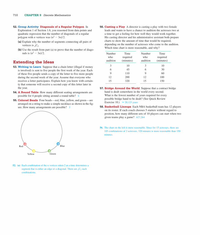
55. Colored Beads Four beads—red, blue, yellow, and green—arearranged on a string to make a simple necklace as shown in the fig-ure. How many arrangements are possible? 3
Red
Yellow Green
Blue
56. Casting a Play A director is casting a play with two femaleleads and wants to have a chance to audition the actresses two at a time to get a feeling for how well they would work together. His casting director and his administrative assistant both preparecharts to show the amount of time that would be required,depending on the number of actresses who come to the audition. Which time chart is more reasonable, and why?
57. Bridge Around the World Suppose that a contract bridgehand is dealt somewhere in the world every second. What is the fewest number of years required for every possible bridge hand to be dealt? (See Quick ReviewExercise 10.) � 20,123 years
58. Basketball Lineups Each NBA basketball team has 12 playerson its roster. If each coach chooses 5 starters without regard toposition, how many different sets of 10 players can start when twogiven teams play a game? 627,264
710 CHAPTER 9 Discrete Mathematics
Number Timewho required
audition (minutes)
3 106 459 110
12 20015 320
Number Timewho required
audition (minutes)
3 106 309 60
12 10015 150
52. (a) Each combination of the n vertices taken 2 at a time determines asegment that is either an edge or a diagonal. There are nC2 suchcombinations.
56. The chart on the left is more reasonable. Since for 15 actresses, there are105 combinations of 2 actresses, 320 minutes is more reasonable than 150minutes.
5144_Demana_Ch09pp699-790 1/13/06 3:06 PM Page 710

SECTION 9.2 The Binomial Theorem 711
9.2The Binomial TheoremWhat you’ll learn about■ Powers of Binomials
■ Pascal’s Triangle
■ The Binomial Theorem
■ Factorial Identities
. . . and whyThe Binomial Theorem is a mar-velous study in combinatorialpatterns.
Powers of BinomialsMany important mathematical discoveries have begun with the study of patterns. Inthis chapter, we want to introduce an important polynomial theorem called theBinomial Theorem, for which we will set the stage by observing some patterns.
If you expand �a � b�n for n � 0, 1, 2, 3, 4, and 5, here is what you get:
�a � b�0 � 1
�a � b�1 � 1a1b0 � 1a0b1
�a � b�2 � 1a2b0 � 2a1b1 � 1a0b2
�a � b�3 � 1a3b0 � 3a2b1 � 3a1b2 � 1a0b3
�a � b�4 � 1a4b0 � 4a3b1 � 6a2b2 � 4a1b3 � 1a0b4
�a � b�5 � 1a5b0 � 5a4b1 � 10a3b2 � 10a2b3 � 5a1b4 � 1a0b5
Can you observe the patterns and predict what the expansion of �a � b�6 will look like?You can probably predict the following:
1. The powers of a will decrease from 6 to 0 by 1’s.
2. The powers of b will increase from 0 to 6 by 1’s.
3. The first two coefficients will be 1 and 6.
4. The last two coefficients will be 6 and 1.
At first you might not see the pattern that would enable you to find the other so-calledbinomial coefficients, but you should see it after the following Exploration.
OBJECTIVEStudents will be able to expand a power of a binomial using the binomial theorem orPascal’s triangle. They will also find thecoefficient of a given term of a binomialexpansion.
MOTIVATEHave students expand (2x � y)4 using thedistributive property. (16x4 � 32x3y � 24x2y2 � 8xy3 � y4)Explain that this section will give them easier ways to do this kind of calculation.
LESSON GUIDEDay 1: Powers of Binomials; Pascal’sTriangleDay 2: The Binomial Theorem; FactorialIdentities
EXPLORATION EXTENSIONSHave the students find the coefficient of ab2
in (a � b)3 by using the distributive propertyor using exponents and without combininglike terms. The relevant terms in the expan-sion will be abb, bab, and bba. There arethree of these terms, so the coefficient ofab2 is 3. Now have the students list all pos-sible ways to have a3b2 and state thecoefficient of this term in the expansionof (a � b)5. (aaabb, aabba, abbaa, …; 10)
EXPLORATION 1 Exploring the Binomial Coefficients
1. Compute 3C0, 3C1, 3C2, and 3C3. Where can you find these numbers in thebinomial expansions above?
2. The expression 4 nCr �0, 1, 2, 3, 4� tells the calculator to compute 4Cr foreach of the numbers r � 0, 1, 2, 3, 4 and display them as a list. Wherecan you find these numbers in the binomial expansions above?
3. Compute 5 nCr �0, 1, 2, 3, 4, 5�. Where can you find these numbers in thebinomial expansions above?
By now you are probably ready to conclude that the binomial coefficients in the expan-sion of �a � b�n are just the values of nCr for r � 0, 1, 2, 3, 4, . . . , n. We also hope youare wondering why this is true.
5144_Demana_Ch09pp699-790 1/13/06 3:06 PM Page 711

712 CHAPTER 9 Discrete Mathematics
The expansion of
�a � b�n � �a � b��a � b��a � b� . . . �a � b��
consists of all possible products that can be formed by taking one letter (either a or b)from each factor �a � b�. The number of ways to form the product arbn�r is exactlythe same as the number of ways to choose r factors to contribute an a, since the rest ofthe factors will obviously contribute a b. The number of ways to choose r factors fromn factors is nCr.
DEFINITION Binomial Coefficient
The binomial coefficients that appear in the expansion of �a � b�n are the values of
nCr for r � 0, 1, 2, 3, . . . , n.
A classical notation for nCr, especially in the context of binomial coefficients, is
(nr ). Both notations are read “n choose r.”
EXAMPLE 1 Using nCr to Expand a BinomialExpand (a � b)5, using a calculator to compute the binomial coefficients.
SOLUTION Enter 5 nCr {0, 1, 2, 3, 4, 5} into the calculator to find the binomialcoefficients for n � 5. The calculator returns the list {1, 5, 10, 10, 5, 1}. Using thesecoefficients, we construct the expansion:
(a � b)5 � 1a5 � 5a4b � 10a3b2 � 10a2b3 � 5ab4 � 1b5.
Now try Exercise 3.
Pascal’s TriangleIf we eliminate the plus signs and the powers of the variables a and b in the “triangular” array of binomial coefficients with which we began this section, we get:
1
1 1
1 2 1
1 3 3 1
1 4 6 4 1
1 5 10 10 5 1. . .. . .. . .
This is called in honor of Blaise Pascal (1623–1662), who used it inhis work but certainly did not discover it. It appeared in 1303 in a Chinese text, thePrecious Mirror, by Chu Shih-chieh, who referred to it even then as a “diagram of theold method for finding eighth and lower powers.”
Pascal’s triangle
TABLE TRICK
You can also use the table display toshow binomial coefficients. For example,let Y1 � 5 nCr X, and set TblStart � 0and �Tbl � 1 to display the binomialcoefficients for (a � b)5.
THE NAME GAME
The fact that Pascal’s triangle was not discovered by Pascal is ironic, but hardlyunusual in the annals of mathematics.We mentioned in Chapter 5 that Herondid not discover Heron’s formula, andPythagoras did not even discover thePythagorean theorem. The history of cal-culus is filled with similar injustices.
n factors
5144_Demana_Ch09pp699-790 1/13/06 3:06 PM Page 712

SECTION 9.2 The Binomial Theorem 713
EXAMPLE 2 Extending Pascal’s TriangleShow how row 5 of Pascal’s triangle can be used to obtain row 6, and use the infor-mation to write the expansion of �x � y�6.
SOLUTION The two outer numbers of every row are 1’s. Each number betweenthem is the sum of the two numbers immediately above it. So row 6 can be foundfrom row 5 as follows:
These are the binomial coefficients for �x � y�6, so
�x � y�6 � x6 � 6x5y � 15x4y2 � 20x3y3 � 15x2y4 � 6xy5 � y6.
Now try Exercise 7.
For convenience, we refer to the top “1” in Pascal’s triangle as row 0. That allows usto associate the numbers along row n with the expansion of �a � b�n.
Pascal’s triangle is so rich in patterns that people still write about them today. One ofthe simplest patterns is the one that we use for getting from one row to the next, as inthe following example.
The technique used in Example 1 to extend Pascal’s triangle depends on the followingrecursion formula.
Here’s a counting argument to explain why it works. Suppose we are choosing r objectsfrom n objects. As we have seen, this can be done in nCr ways. Now identify one of then objects with a special tag. How many ways can we choose r objects if the taggedobject is among them? Well, we have r � 1 objects yet to be chosen from among then � 1 that are untagged, so n�1Cr �1. How many ways can we choose r objects if thetagged object is not among them? This time we must choose all r objects from amongthe n � 1 without tags, so n �1Cr . Since our selection of r objects must either containthe tagged object or not contain it, n�1Cr �1 � n�1Cr counts all the possibilities with nooverlap. Therefore, nCr � n�1Cr�1 � n�1Cr .
It is not necessary to construct Pascal’s triangle to find specific binomial coefficients,
since we already have a formula for computing them: nCr � ( ) � r!�n
n�
!r�!
. This
formula can be used to give an algebraic formula for the recursion formula above, but wewill leave that as an exercise for the end of the section.
nr
Recursion Formula for Pascal’s Triangle
( ) � ( ) � ( ) or, equivalently, nCr � n�1Cr�1 � n�1Crn � 1
rn � 1r � 1
nr
5144_Demana_Ch09pp699-790 1/13/06 3:06 PM Page 713

714 CHAPTER 9 Discrete Mathematics
The Binomial TheoremWe now state formally the theorem about expanding powers of binomials, known as the
Binomial Theorem. For tradition’s sake, we will use the symbol ( ) instead of nCr.nr
ALERT
Students often make sign errors when theyapply the binomial theorem to an expres-sion of the form (a � b)n. Emphasize thatthis must be interpreted as (a � (�b))n.
EXAMPLE 3 Computing Binomial CoefficientsFind the coefficient of x10 in the expansion of �x � 2�15.
SOLUTION The only term in the expansion that we need to deal with is 15C10 x1025.This is
1105!5!!
• 25 • x10 � 3003 • 32 • x10 � 96,096 x10.
The coefficient of x10 is 96,096. Now try Exercise 15.
The Binomial Theorem
For any positive integer n,
�a � b�n � (n0)an � (n
1)an�1b � . . . � (nr )an�rbr � . . . � (n
n )bn,
where
(nr ) � nCr �
r!�nn�
!r�!
.
EXAMPLE 4 Expanding a BinomialExpand �2x � y2�4.
SOLUTION We use the Binomial Theorem to expand �a � b�4 where a � 2x andb � �y2.
�a � b�4 � a4 � 4a3b � 6a2b2 � 4ab3 � b4
�2x � y2�4� �2x�4
� 4�2x�3��y2� � 6�2x�2��y2�2
� 4�2x���y2�3� ��y2�4
� 16x4 � 32x3y2 � 24x2y4 � 8xy6 � y8
Now try Exercise 17.
Factorial IdentitiesExpressions involving factorials combine to give some interesting identities, most ofthem relying on the basic identities shown below (actually two versions of the sameidentity).
Basic Factorial Identities
For any integer n � 1, n! � n(n � 1)!
For any integer n � 0, (n � 1)! � (n � 1)n!
FOLLOW-UP
Ask how many terms the expanded formof (x � y)23 has. (24)
ASSIGNMENT GUIDE
Day 1: Ex. 1–15 odd, 27, 28Day 2: Ex. 17–25 odd, 29, 34–40
COOPERATIVE LEARNING
Group Activity: Ex. 42
NOTES ON EXERCISES
Ex. 9–12 should be done first without a grapher in order to familiarize students with the algebraic manipulations required to calculate binomial coefficients.Ex. 29–31, 33–34, and 43–45 requirestudents to prove various statementsrelating to binomial coefficients or theBinomial Theorem.Ex. 35–40 provide practice for standardizedtests.
ONGOING ASSESSMENT
Self-Assessment: Ex. 3, 7, 15, 17, 33Embedded Assessment: Ex. 32, 41
THE BINOMIAL THEOREM
IN � NOTATION
For those who are already familiar withsummation notation, here is how theBinomial Theorem looks:
(a � b)n � n
r�0( )an�rbr.
Those who are not familiar with thisnotation will learn about it in Section 9.4.
nr
5144_Demana_Ch09pp699-790 1/13/06 3:06 PM Page 714

SECTION 9.2 The Binomial Theorem 715
EXAMPLE 5 Proving an Identity with Factorials
Prove that ( ) � ( ) � n for all integers n � 2.
SOLUTION
( ) � ( ) � 2!(n
(n�
�
11)�
!2)!
� 2!(n
n�
!2)!
Combination counting formula
� (n�
21()n(n
�
)(n1�
)!1)!
�n(n
2�
(n1�
)(n2�
)!2)!
Basic factorial identities
� n2
2� n �
n2
2� n
� 22n
� n Now try Exercise 33.
n2
n � 12
n2
n � 12
QUICK REVIEW 9.2 (Prerequisite skill Section A.2)
In Exercises 1–10, use the distributive property to expand the binomial.
1. �x � y�2 x2 � 2xy � y2 2. �a � b�2 a2 � 2ab � b2
3. �5x � y�2 25x2 � 10xy � y2 4. �a � 3b�2a2 � 6ab � 9b2
5. �3s � 2t�2 6. �3p � 4q�2
7. �u � v�3 8. �b � c�3
9. �2x � 3y�3 10. �4m � 3n�3
SECTION 9.2 EXERCISES
In Exercises 1–4, expand the binomial using a calculator to find thebinomial coefficients.
1. (a � b)4 2. (a � b)6
3. (x � y)7 4. (x � y)10
In Exercises 5–8, expand the binomial using Pascal’s triangle to findthe coefficients.
5. �x � y�3 6. �x � y�5
7. �p � q�8 8. �p � q�9
In Exercises 9–12, evaluate the expression by hand (using the formula)before checking your answer on a grapher.
9. ( ) 36 10. ( ) 1365
11. ( ) 1 12. ( ) 11660
166166
1511
92
In Exercises 13–16, find the coefficient of the given term in the binomial expansion.
13. x11y3 term, �x � y�14 364 14. x5y8 term, �x � y�13 1287
15. x4 term, �x � 2�12 126,720 16. x7 term, �x � 3�11 26,730
In Exercises 17–20, use the Binomial Theorem to find a polynomial expansion for the function.
17. f �x� � �x � 2�5 18. g�x� � �x � 3�6
19. h�x� � �2x � 1�7 20. f �x� � �3x � 4�5
In Exercises 21–26, use the Binomial Theorem to expand each expression.
21. �2x � y�4 22. �2y � 3x�5
23. �x� � y��6 24. �x� � 3��4
25. �x�2 � 3�5 26. �a � b�3�7
27. Determine the largest integer n for which your calculator willcompute n!.
5144_Demana_Ch09pp699-790 1/13/06 3:06 PM Page 715

28. Determine the largest integer n for which your calculator
will compute ( ).29. Prove that ( ) � ( ) � n for all integers n � 1.
30. Prove that ( ) � ( ) for all integers n � r � 0.
31. Use the formula ( ) � r!�n
n�
!r�!
to prove that
( ) � ( ) � ( ). (This is the pattern in Pascal’s
triangle that appears in Example 2.)
32. Find a counterexample to show that each statement is false.
(a) �n � m�! � n! � m!
(b) �nm�! � n!m!
33. Prove that ( ) � ( ) � n2 for all integers n � 2.
34. Prove that ( ) � ( ) � n2 for all integers n � 2.
Standardized Test Questions35. True or False The coefficients in the polynomial expansion of
(x � y)50 alternate in sign. Justify your answer.
36. True or False The sum of any row of Pascal’s triangle is aneven integer. Justify your answer.
You may use a graphing calculator when evaluating Exercises 37–40.
37. Multiple Choice What is the coefficient of x4 in the expansionof (2x � 1)8? C
(A) 16
(B) 256
(C) 1120
(D) 1680
(E) 26,680
38. Multiple Choice Which of the following numbers does notappear on row 10 of Pascal’s Triangle? B
(A) 1
(B) 5
(C) 10
(D) 120
(E) 252
n � 1n � 1
nn � 2
n � 12
n2
n � 1r
n � 1r � 1
nr
nr
nn � r
nr
nn � 1
n1
n100
39. Multiple Choice The sum of the coefficients of(3x � 2y)10 is A
(A) 1
(B) 1024
(C) 58,025
(D) 59,049
(E) 9,765,625
40. Multiple Choice (x � y)3 � (x � y)3 � D
(A) 0
(B) 2x3
(C) 2x3 � 2y3
(D) 2x3 � 6xy2
(E) 6x2y � 2y3
Explorations41. Triangular Numbers Numbers of the form 1 � 2 � . . . � n
are called because they count numbers intriangular arrays, as shown below:
triangular numbers
716 CHAPTER 9 Discrete Mathematics
(a) Compute the first 10 triangular numbers.
(b) Where do the triangular numbers appear in Pascal’s triangle?
(c) Writing to Learn Explain why the diagram below showsthat the nth triangular number can be written as n�n � 1��2.
(d) Write the formula in part (c) as a binomial coefficient. (This iswhy the triangular numbers appear as they do in Pascal’s triangle.)
5144_Demana_Ch09pp699-790 1/13/06 3:06 PM Page 716

SECTION 9.2 The Binomial Theorem 717
42. Group Activity Exploring Pascal’s Triangle Break intogroups of two or three. Just by looking at patterns in Pascal’s triangle, guess the answers to the following questions. (It is easierto make a conjecture from a pattern than it is to construct aproof!)
(a) What positive integer appears the least number of times? 2
(b) What number appears the greatest number of times? 1
(c) Is there any positive integer that does not appear in Pascal’s triangle? no
(d) If you go along any row alternately adding and subtracting thenumbers, what is the result? 0
(e) If p is a prime number, what do all the interior numbers alongthe pth row have in common? All are divisible by p.
(f) Which rows have all even interior numbers?
(g) Which rows have all odd numbers?
(h) What other patterns can you find? Share your discoveries withthe other groups.
Extending the Ideas43. Use the Binomial Theorem to prove that the sum of the entries
along the nth row of Pascal’s triangle is 2n. That is,
( ) � ( ) � ( ) � . . . � ( ) � 2n.
[Hint: Use the Binomial Theorem to expand (1 � 1)n.]
44. Use the Binomial Theorem to prove that the alternating sum alongany row of Pascal’s triangle is zero. That is,
( ) � ( ) � ( ) � . . . � ��1�n( ) � 0.
45. Use the Binomial Theorem to prove that
( ) � 2( ) � 4( ) � . . . � 2n ( ) � 3n. nn
n2
n1
n0
nn
n2
n1
n0
nn
n2
n1
n0
42. (f) Rows that are powers of 2: 2, 4, 8, 16, etc. (g) Rows that are 1 less than a power of 2: 1, 3, 7, 15, etc.
43. 2n � (1 � 1)n � � 1n10 � � 1n�111 � � 1n�212 � ... � � 101n � � � � � � � ... � � nn
n2
n1
n0
nn
n2
n1
n0
5144_Demana_Ch09pp699-790 1/13/06 3:06 PM Page 717

718 CHAPTER 9 Discrete Mathematics
9.3ProbabilityWhat you’ll learn about■ Sample Spaces and Probability
Functions
■ Determining Probabilities
■ Venn Diagrams and TreeDiagrams
■ Conditional Probability
■ Binomial Distributions
. . . and whyEveryone should know howmathematical the “laws ofchance” really are.
Sample Spaces and Probability FunctionsMost people have an intuitive sense of probability. Unfortunately, this sense is notoften based on a foundation of mathematical principles, so people become victims ofscams, misleading statistics, and false advertising. In this lesson, we want to build onyour intuitive sense of probability and give it a mathematical foundation.
EXAMPLE 1 Testing Your Intuition About ProbabilityFind the probability of each of the following events.
(a) Tossing a head on one toss of a fair coin.
(b) Tossing two heads in a row on two tosses of a fair coin.
(c) Drawing a queen from a standard deck of 52 cards.
(d) Rolling a sum of 4 on a single roll of two fair dice.
(e) Guessing all 6 numbers in a state lottery that requires you to pick 6 numbersbetween 1 and 46, inclusive.
SOLUTION
(a) There are two equally likely outcomes: �T, H�. The probability is 1�2.
(b) There are four equally likely outcomes: �TT, TH, HT, HH�. The probability is 1�4.
(c) There are 52 equally likely outcomes, 4 of which are queens. The probability is4�52, or 1�13.
(d) By the Multiplication Principle of Counting (Section 9.1), there are 6 � 6 � 36 equally likely outcomes. Of these, three ��1, 3�, �3, 1�, �2, 2�� yield asum of 4 (Figure 9.2). The probability is 3�36, or 1�12.
(e) There are 46C6 � 9,366,819 equally likely ways that 6 numbers can be chosenfrom 46 numbers without regard to order. Only one of these choices wins the lot-tery. The probability is 1�9,366,819 � 0.00000010676. Now try Exercise 5.
FIGURE 9.2 A sum of 4 on a roll of two dice. (Example 1d)
Notice that in each of these cases we first counted the number of possible outcomes ofthe experiment in question. The set of all possible outcomes of an experiment is the
of the experiment. An is a subset of the sample space. Each of our sample spaces consisted of a finite number of , which enabledus to find the probability of an event by counting.
equally likely outcomeseventsample space
Probability of an Event (Equally Likely Outcomes)
If E is an event in a finite, nonempty sample space S of equally likely outcomes, thenthe of the event E is
P(E) � .the number of outcomes in Ethe number of outcomes in S
probability
5144_Demana_Ch09pp699-790 1/13/06 3:06 PM Page 718

SECTION 9.3 Probability 719
TEACHING NOTE
Probability theory got its start as an analysisof games of chance. It has grown to includemany industrial and scientific applications.
OBJECTIVE
Students will be able to identify a samplespace and calculate probabilities and condi-tional probabilities in sample spaces withequally likely or unequally likely outcomes.
MOTIVATE
Ask which is more likely when tossing twodice: a sum of 3 or a sum of 5? (5)
LESSON GUIDE
Day 1: Sample Spaces and ProbabilityFunctions; Determining Probabilities; VennDiagrams and Tree Diagrams.Day 2: Conditional Probability; BinomialDistributions.
The hypothesis of equally likely outcomes is critical here. Many people guess wronglyon the probability in Example 1d because they figure that there are 11 possible out-comes for the sum on two fair dice: �2, 3, 4, 5, 6, 7, 8, 9, 10, 11, 12� and that 4 is oneof them. (That reasoning is correct so far.) The reason that 1�11 is not the probabilityof rolling a sum of 4 is that all those sums are not equally likely.
On the other hand, we can assign probabilities to the 11 outcomes in this smaller sam-ple space in a way that is consistent with the number of ways each total can occur. Thetable below shows a , in which each outcome is assigned aunique probability by a probability function.
Outcome Probability
2 1�36
3 2�36
4 3�36
5 4�36
6 5�36
7 6�36
8 5�36
9 4�36
10 3�36
11 2�36
12 1�36
We see that the outcomes are not equally likely, but we can find the probabilities ofevents by adding up the probabilities of the outcomes in the event, as in the followingexample.
EXAMPLE 2 Rolling the DiceFind the probability of rolling a sum divisible by 3 on a single roll of two fair dice.
SOLUTION The event E consists of the outcomes �3, 6, 9, 12�. To get the proba-bility of E we add up the probabilities of the outcomes in E (see the table of the prob-ability distribution):
P�E� � 326 �
356 �
346 �
316 �
1326 �
13
.
Now try Exercise 7.
Notice that this method would also have worked just fine with our 36-outcome samplespace, in which every outcome has probability 1/36. In general, it is easier to work withsample spaces of equally likely events because it is not necessary to write out the prob-ability distribution. When outcomes do have unequal probabilities, we need to knowwhat probabilities to assign to the outcomes.
probability distribution
IS PROBABILITY JUST FOR GAMES?
Probability theory got its start in lettersbetween Blaise Pascal (1623–1662) andPierre de Fermat (1601–1665) concerninggames of chance, but it has come a longway since then. Modern mathematicianslike David Blackwell (1919), the firstAfrican-American to receive a fellowshipto the Institute for Advanced Study atPrinceton, have greatly extended boththe theory and the applications ofprobability, especially in the areas ofstatistics, quantum physics, and information theory. Moreover, the workof John Von Neumann (1903–1957) hasled to a separate branch of modern discrete mathematics that really isabout games, called Game Theory.
5144_Demana_Ch09pp699-790 1/13/06 3:06 PM Page 719
720 CHAPTER 9 Discrete Mathematics
The probability of any event can then be defined in terms of the probability function.
EMPTY SET
A set with no elements is the emptyset, denoted by �.
DEFINITION Probability Function
A is a function P that assigns a real number to each outcomein a sample space S subject to the following conditions:
1. 0 P�O� 1 for every outcome O;
2. the sum of the probabilities of all outcomes in S is 1;
3. P��� � 0.
probability function
Probability of an Event (Outcomes not Equally Likely)
Let S be a finite, nonempty sample space in which every outcome has a probabilityassigned to it by a probability function P. If E is any event in S, the ofthe event E is the sum of the probabilities of all the outcomes contained in E.
probability
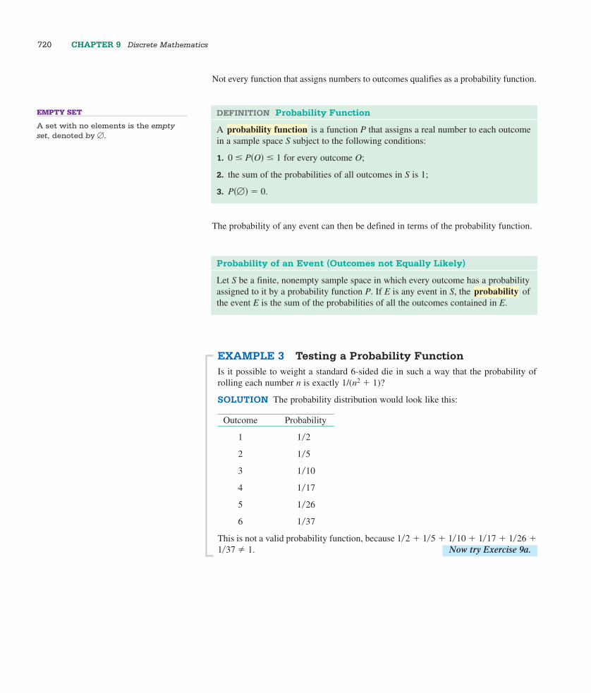
Not every function that assigns numbers to outcomes qualifies as a probability function.
EXAMPLE 3 Testing a Probability FunctionIs it possible to weight a standard 6-sided die in such a way that the probability ofrolling each number n is exactly 1/(n2 � 1)?
SOLUTION The probability distribution would look like this:
Outcome Probability
1 1�2
2 1�5
3 1�10
4 1�17
5 1�26
6 1�37
This is not a valid probability function, because 1�2 � 1�5 � 1�10 � 1�17 � 1�26 �1�37 � 1. Now try Exercise 9a.
5144_Demana_Ch09pp699-790 1/13/06 3:06 PM Page 720

SECTION 9.3 Probability 721
EXAMPLE 4 Choosing Chocolates, Sample Space ISal opens a box of a dozen chocolate cremes and generously offers two of them toVal. Val likes vanilla cremes the best, but all the chocolates look alike on the outside.If four of the twelve cremes are vanilla, what is the probability that both of Val’s picksturn out to be vanilla?
SOLUTION The experiment in question is the selection of two chocolates, withoutregard to order, from a box of 12. There are 12C2 � 66 outcomes of this experiment,and all of them are equally likely. We can therefore determine the probability bycounting.
The event E consists of all possible pairs of 2 vanilla cremes that can be chosen, with-out regard to order, from 4 vanilla cremes available. There are 4C2 � 6 ways to formsuch pairs.
Therefore, P�E� � 6�66 � 1�11. Now try Exercise 25.
Many probability problems require that we think of events happening in succession,often with the occurrence of one event affecting the probability of the occurrence ofanother event. In these cases, we use a law of probability called the MultiplicationPrinciple of Probability.
Determining ProbabilitiesIt is not always easy to determine probabilities, but the arithmetic involved is fairlysimple. It usually comes down to multiplication, addition, and (most importantly)counting. Here is the strategy we will follow:
Strategy for Determining Probabilities
1. Determine the sample space of all possible outcomes. When possible,choose outcomes that are equally likely.
2. If the sample space has equally likely outcomes, the probability of an eventE is determined by counting:
P�E� � the number of outcomes in E
the number of outcomes in S.
3. If the sample space does not have equally likely outcomes, determine theprobability function. (This is not always easy to do.) Check to be sure thatthe conditions of a probability function are satisfied. Then the probability ofan event E is determined by adding up the probabilities of all the outcomescontained in E.
5144_Demana_Ch09pp699-790 1/13/06 3:06 PM Page 721

722 CHAPTER 9 Discrete Mathematics
Multiplication Principle of Probability
Suppose an event A has probability p1 and an event B has probability p2 under theassumption that A occurs. Then the probability that both A and B occur is p1p2.
If the events A and B are , we can omit the phrase “under the assumptionthat A occurs,” since that assumption would not matter.
As an example of this principle at work, we will solve the same problem as that posedin Example 4, this time using a sample space that appears at first to be simpler, butwhich consists of events that are not equally likely.
EXAMPLE 5 Choosing Chocolates, Sample Space IISal opens a box of a dozen chocolate cremes and generously offers two of them toVal. Val likes vanilla cremes the best, but all the chocolates look alike on the outside.If four of the twelve cremes are vanilla, what is the probability that both of Val’s picksturn out to be vanilla?
SOLUTION As far as Val is concerned, there are two kinds of chocolate cremes:vanilla �V � and unvanilla �U�. When choosing two chocolates, there are four possibleoutcomes: VV, VU, UV, and UU. We need to determine the probability of the out-come VV.
Notice that these four outcomes are not equally likely! There are twice as many Uchocolates as V chocolates. So we need to consider the distribution of probabilities,and we may as well begin with P�VV �, as that is the probability we seek.
The probability of picking a vanilla creme on the first draw is 4�12. The probability ofpicking a vanilla creme on the second draw, under the assumption that a vanilla cremewas drawn on the first, is 3�11. By the Multiplication Principle, the probability of draw-ing a vanilla creme on both draws is
142 •
131 �
111.
Since this is the probability we are looking for, we do not need to compute the prob-abilities of the other outcomes. However, you should verify that the other probabili-ties would be:
P�VU � � 142 •
181 �
383
P�UV � � 182 •
141 �
383
P�UU � � 182 •
171 �
1343
Notice that P�VV � � P�VU � � P�UV � � P�UU � � �1�11� � �8�33� � �8�33� ��14�33� � 1, so the probability function checks out. Now try Exercise 33.
independent
ORDERED OR UNORDERED?
Notice that in Example 4 we had asample space in which order was dis-regarded, whereas in Example 5 wehave a sample space in which ordermatters. (For example, UV and VU aredistinct outcomes.) The order mattersin Example 5 because we are consider-ing the probabilities of two events (firstdraw, second draw), one of which affectsthe other. In Example 4, we are simplycounting unordered combinations.
5144_Demana_Ch09pp699-790 1/13/06 3:06 PM Page 722

SECTION 9.3 Probability 723
JOHN VENN
John Venn (1834–1923) was an Englishlogician and clergyman, just like hiscontemporary, Charles L. Dodgson.Although both men used overlapping circles to illustrate their logical syllo-gisms, it is Venn whose name lives onin connection with these diagrams.Dodgson’s name barely lives on at all,and yet he is far the more famous ofthe two: under the pen name LewisCarroll, he wrote Alice’s Adventures inWonderland and Through the LookingGlass.
FIGURE 9.3 A Venn diagram forExample 6. The overlapping region commonto both circles represents “girls who playsports.” The region outside both circles (butinside the rectangle) represents “boys whodo not play sports.”
Girls Sports
FIGURE 9.4 A Venn diagram forExample 6 with the probabilities filled in.
Girls Sports
0.27 0.27 0.35
0.11
Venn Diagrams and Tree DiagramsWe have seen many instances in which geometric models help us to understand alge-braic models more easily, and probability theory is yet another setting in which this istrue. , associated mainly with the world of set theory, are good for visualizing relationships among events within sample spaces. , whichwe first met in Section 9.1 as a way to visualize the Multiplication Principle ofCounting, are good for visualizing the Multiplication Principle of Probability.
EXAMPLE 6 Using a Venn DiagramIn a large high school, 54% of the students are girls and 62% of the students playsports. Half of the girls at the school play sports.
(a) What percentage of the students who play sports are boys?
(b) If a student is chosen at random, what is the probability that it is a boy who doesnot play sports?
SOLUTION To organize the categories, we draw a large rectangle to represent thesample space (all students at the school) and two overlapping regions to represent“girls” and “sports” (Figure 9.3). We fill in the percentages (Figure 9.4) using the fol-lowing logic:
• The overlapping (green) region contains half the girls, or (0.5)(54%) � 27% of thestudents.
• The yellow region (the rest of the girls) then contains (54 – 27)% � 27% of the students.
• The blue region (the rest of the sports players) then contains (62 – 27)% � 35% ofthe students.
• The white region (the rest of the students) then contains (100 – 89)% � 11% of thestudents. These are boys who do not play sports.
We can now answer the two questions by looking at the Venn diagram.
(a) We see from the diagram that the ratio of boys who play sports to all students who
play sports is 00..3652
, which is about 56.45%.
(b) We see that 11% of the students are boys who do not play sports, so 0.11 is theprobability. Now try Exercises 27a–d.
Tree diagramsVenn diagrams
5144_Demana_Ch09pp699-790 1/13/06 3:06 PM Page 723

724 CHAPTER 9 Discrete Mathematics
Conditional ProbabilityThe probability of drawing a chocolate chip cookie in Example 7 is an example of
, since the “cookie” probability is on the “jar”outcome. A convenient symbol to use with conditional probability is P�A �B�, pro-nounced “P of A given B,” meaning “the probability of the event A, given that event Boccurs.” In the cookie jars of Example 7,
P�chocolate chip � jar A� � 24
and P�chocolate chip � jar B� � 1.
(In the tree diagram, these are the probabilities along the branches that come out of thetwo jars, not the probabilities at the ends of the branches.)
The Multiplication Principle of Probability can be stated succinctly with this notationas follows:
P�A and B� � P�A� • P�B �A�.
This is how we found the numbers at the ends of the branches in Figure 9.6.
As our final example of a probability problem, we will show how to use this formula ina different but equivalent form, sometimes called the formula:
conditional probability
dependentconditional probability
EXAMPLE 7 Using a Tree DiagramTwo identical cookie jars are on a counter. Jar A contains 2 chocolate chip and 2 peanutbutter cookies, while jar B contains 1 chocolate chip cookie. We select a cookie at ran-dom. What is the probability that it is a chocolate chip cookie?
SOLUTION It is tempting to say 3�5, since there are 5 cookies in all, 3 of whichare chocolate chip. Indeed, this would be the answer if all the cookies were in thesame jar. However, the fact that they are in different jars means that the 5 cookies arenot equally likely outcomes. That lone chocolate chip cookie in jar B has a much bet-ter chance of being chosen than any of the cookies in jar A. We need to think of thisas a two-step experiment: first pick a jar, then pick a cookie from that jar.
Figure 9.5 gives a visualization of the two-step process. In Figure 9.6, we have filledin the probabilities along each branch, first of picking the jar, then of picking thecookie. The probability at the end of each branch is obtained by multiplying the prob-abilities from the root to the branch. (This is the Multiplication Principle.) Notice thatthe probabilities of the 5 cookies (as predicted) are not equal.
The event “chocolate chip” is a set containing three outcomes. We add their proba-bilities together to get the correct probability:
P�chocolate chip� � 0.125 � 0.125 � 0.5 � 0.75. Now try Exercise 29.FIGURE 9.6 The tree diagram forExample 7 with the probabilities filled in.Notice that the five cookies are not equallylikely to be drawn. Notice also that the prob-abilities of the five cookies do add up to 1.
JarA
JarB CC
PB
CC
CC
PB
0.5
0.5
0.25
0.25
0.25
0.25
0.125
0.125
0.125
0.125
0.51
FIGURE 9.5 A tree diagram for Example 7.
JarA
JarB CC
PB
CC
CC
PB
Conditional Probability Formula
If the event B depends on the event A, then P(B � A) � P(A
Pa(And
)B)
.
ALERT
Many students, when faced with a newprobability experiment, will begin manip-ulating probability formulas before theyunderstand the experiment. Ask them tolist a few elements of the sample space tobetter understand the problem. Then theycan begin calculating the probability ofthe event.
5144_Demana_Ch09pp699-790 1/13/06 3:06 PM Page 724

SECTION 9.3 Probability 725
EXAMPLE 8 Using the Conditional Probability FormulaSuppose we have drawn a cookie at random from one of the jars described inExample 7. Given that it is chocolate chip, what is the probability that it came fromjar A?
SOLUTION By the formula,
P� jar A �chocolate chip� �
� �1�
02.�7�25�4�
� 00..2755
� 13
Now try Exercise 31.
P� jar A and chocolate chip�
P�chocolate chip�
EXPLORATION 1 Testing Positive for HIV
As of the year 2003, the probability of an adult in the United States havingHIV/AIDS was 0.006 (Source: 2004 CIA World Factbook). The ELISA test isused to detect the virus antibody in blood. If the antibody is present, the testreports positive with probability 0.997 and negative with probability 0.003. Ifthe antibody is not present, the test reports positive with probability 0.015 andnegative with probability 0.985.
1. Draw a tree diagram with branches to nodes “antibody present” and “anti-body absent” branching from the root. Fill in the probabilities for NorthAmerican adults (age 15–49) along the branches. (Note that these twoprobabilities must add up to 1.)
2. From the node at the end of each of the two branches, draw branches to“positive” and “negative.” Fill in the probabilities along the branches.
3. Use the Multiplication Principle to fill in the probabilities at the ends ofthe four branches. Check to see that they add up to 1.
4. Find the probability of a positive test result. (Note that this event consistsof two outcomes). 0.02089
5. Use the conditional probability formula to find the probability that a per-son with a positive test result actually has the antibody, i.e., P(antibodypresent �positive). � 0.286
You might be surprised that the answer to part 5 is so low, but it should becompared with the probability of the antibody being present before seeing thepositive test result, which was 0.006. Nonetheless, that is why a positiveELISA test is followed by further testing before a diagnosis of HIV/AIDS ismade. This is the case with many diagnostic tests.
EXPLORATION EXTENSIONS
A reporter announces that there is an 80%chance of a thunderstorm tomorrow, andif the thunderstorm materializes there is a14% chance that it will produce a torna-do. What is the probability that there willbe a tornado tomorrow? (11.2%)
What is the probability that there is astorm, but that it does not produce a tornado? (68.8%)
5144_Demana_Ch09pp699-790 1/13/06 3:06 PM Page 725

726 CHAPTER 9 Discrete Mathematics
Did the form of those answers look a little familiar? Watch what they look like whenwe let p � 1�6 and q � 5�6:
P�four 3’s� � p4
P�no 3’s� � q4
P�two 3’s� � ( ) p2q2
You can probably recognize these as three of the terms in the expansion of �p � q�4.This is no coincidence. In fact, the terms in the expansion
�p � q�4 � p4 � 4p3q1 � 6p2q2 � 4p1q3 � q4
give the exact probabilities of 4, 3, 2, 1, and 0 threes (respectively) when we toss a fairdie four times! That is why this is called a binomial probability distribution. The gen-eral theorem follows.
42
EXAMPLE 9 Repeating a Simple ExperimentWe roll a fair die four times. Find the probability that we roll:
(a) all 3’s. (b) no 3’s. (c) exactly two 3’s.
SOLUTION
(a) We have a probability 1�6 of rolling a 3 each time. By the MultiplicationPrinciple, the probability of rolling a 3 all four times is �1�6�4 � 0.00077.
(b) There is a probability 5�6 of rolling something other than 3 each time. By theMultiplication Principle, the probability of rolling a non-3 all four times is �5�6�4 � 0.48225.
(c) The probability of rolling two 3’s followed by two non-3’s (again by theMultiplication Principle) is �1�6�2�5�6�2 � 0.01929. However, that is not the onlyoutcome we must consider. In fact, the two 3’s could occur
anywhere among the four rolls, in exactly ( ) � 6 ways. That gives us 6 outcomes,
each with probability �1�6�2�5�6�2. The probability of the event “exactly two 3’s”
is therefore ( )�1�6�2�5�6�2 � 0.11574.
Now try Exercise 47.
42
42
Binomial DistributionsWe noted in our “Strategy for Determining Probabilities” that it is not always easy todetermine a probability distribution for a sample space with unequal probabilities. Aninteresting exception for those who have studied the Binomial Theorem (Section 9.2)is the binomial distribution.
5144_Demana_Ch09pp699-790 1/13/06 3:06 PM Page 726

SECTION 9.3 Probability 727
Number of successes out ofn independent repetitions Probability
n pn
n � 1 ( nn � 1)pn�1q
.
.
....
r (nr )pr qn�r
.
.
....
1 (n1)pqn�1
0 qn
THEOREM Binomial Distribution
Suppose an experiment consists of n independent repetitions of an experiment withtwo outcomes, called “success” and “failure.” Let P(success) � p and P(failure) � q.(Note that q � 1 � p.)
Then the terms in the binomial expansion of �p � q�n give the respective probabili-ties of exactly n, n � 1, . . . , 2, 1, 0 successes. The distribution is shown below:
EXAMPLE 10 Shooting Free ThrowsSuppose Michael makes 90% of his free throws. If he shoots 20 free throws, and ifhis chance of making each one is independent of the other shots (an assumption youmight question in a game situation), what is the probability that he makes
(a) all 20?
(b) exactly 18?
(c) at least 18?
SOLUTION We could get the probabilities of all possible outcomes by expanding�0.9 � 0.1�20, but that is not necessary in order to answer these three questions. Wejust need to compute three specific terms.
(a) P�20 successes� � �0.9�20 � 0.12158
(b) P�18 successes� � ( ) �0.9�18�0.1�2 � 0.28518
(c) P�at least 18 successes� � P�18� � P�19� � P�20�
� ( )�0.9�18�0.1�2 � ( )�0.9�19 �0.1� � �0.9�20
� 0.6769 Now try Exercise 49.
2019
2018
2018
BINOMIAL PROBABILITIES
ON A CALCULATOR
Your calculator might be programmed tofind values for the binomial probabilitydistribution function (binompdf). Thesolutions to Example 10 in one calcula-tor syntax, for example, could beobtained by:
(a) binompdf(20, .9, 20) (20 repetitions,0.9 probability, 20 successes)
(b) binompdf(20, .9, 18) (20 repetitions,0.9 probability, 18 successes)
(c) 1 � binomcdf(20, .9, 17) (1 minus thecumulative probability of 17 or fewersuccesses)
Check your owner’s manual for moreinformation.
FOLLOW-UP
Assume that the probability that a new-born child is a particular sex is 50%. In afamily of four children, what is the proba-bility of the given event?
a. All the children are girls. (1/16)
b. No two of the children are the same sex. (0)
c. All the children are boys or girls. (1)
d. A least two of the children are boys.(11/16)
ASSIGNMENT GUIDE
Day 1: Ex. 3–27, multiples of 3Day 2: Ex. 30–48, multiples of 3, 51–56
COOPERATIVE LEARNING
Group Activity: Ex. 32, 60
NOTES ON EXERCISES
Ex. 1–26 are typical probability practice,problems.Ex. 43–50 are binomial probabilities.Ex. 51–56 provide practice for standard-ized tests.Ex. 61 and 62 are expected value problems.
ONGOING ASSESSMENT
Self-Assessment: Ex. 5, 7, 9, 25, 27, 29,31, 33, 47, 49Embedded Assessment: Ex. 9, 37, 42,57, 62
5144_Demana_Ch09pp699-790 1/13/06 3:06 PM Page 727

728 CHAPTER 9 Discrete Mathematics
QUICK REVIEW 9.3 (Prerequisite skill Section 9.1)
In Exercises 1–8, tell how many outcomes are possible for the experiment.
1. A single coin is tossed. 2
2. A single 6-sided die is rolled. 6
3. Three different coins are tossed. 8
4. Three different 6-sided dice are rolled. 216
5. Five different cards are drawn from a standard deck of 52.
6. Two chips are drawn simultaneously without replacementfrom a jar containing 10 chips. 45
7. Five people are lined up for a photograph. 120
8. Three-digit numbers are formed from the numbers�1, 2, 3, 4, 5� without repetition. 60
In Exercises 9 and 10, evaluate the expression by pencil and paper.Verify your answer with a calculator.
9. 1
5
0
CC
3
3
112 10.
1
5
0
CC
2
2
29
SECTION 9.3 EXERCISES
In Exercises 1–8, a red die and a green die have been rolled. What isthe probability of the event?
1. The sum is 9. 1/9 2. The sum is even. 1/2
3. The number on the red die is greater than the number on the greendie. 5/12
4. The sum is less than 10. 5/6 5. Both numbers are odd. 1/4
6. Both numbers are even. 1/4 7. The sum is prime. 5/12
8. The sum is 7 or 11. 2/9
9. Writing to Learn Alrik’s gerbil cage has four compartments,A, B, C, and D. After careful observation, he estimates the propor-tion of time the gerbil spends in each compartment and constructsthe table below.
In Exercises 11–16, a single candy of this type is selected at randomfrom a newly-opened bag. What is the probability that the candy hasthe given color(s)?
11. Brown or tan 0.4 12. Red, green, or orange 0.4
13. Red 0.2 14. Not red 0.8
15. Neither orange nor yellow 16. Neither brown nor tan 0.6
A peanut version of the same candy has all the same colors except tan.The proportions of the peanut version are given in the following table.
Compartment A B C D
Proportion 0.25 0.20 0.35 0.30
Color Brown Red Yellow Green Orange Tan
Proportion 0.3 0.2 0.2 0.1 0.1 0.1
Color Brown Red Yellow Green Orange
Proportion 0.3 0.2 0.2 0.2 0.1
(a) Is this a valid probability function? Explain.
(b) Is there a problem with Alrik’s reasoning? Explain.
10. (Continuation of Exercise 9) Suppose Alrik determines that hisgerbil spends time in the four compartments A, B, C, and D in theratio 4:3:2:1. What proportions should he fill in the table above? Isthis a valid probability function? 0.4, 0.3, 0.2, 0.1; yes
The maker of a popular chocolate candy that is covered in a thin col-ored shell has released information about the overall color proportionsin its production of the candy, which is summarized in the followingtable.
In Exercises 17–22, a candy of this type is selected at random fromeach of two newly-opened bags. What is the probability that the twocandies have the given color(s)?
17. Both are brown. 0.09 18. Both are orange. 0.01
19. One is red, and the other is green. 0.08
20. The first is brown, and the second is yellow. 0.06
21. Neither is yellow. 0.64
22. The first is not red, and the second is not orange. 0.72
Exercises 23–32 concern a version of the card game “bid Euchre” thatuses a pack of 24 cards, consisting of ace, king, queen, jack, 10, and 9in each of the four suits (spades, hearts, diamonds, and clubs). In bidEuchre, a hand consists of 6 cards. Find the probability of each event.
23. Euchre A hand is all spades. 1/134,596
24. Euchre All six cards are from the same suit. 1/33,649
25. Euchre A hand includes all four aces. 5/3542
5. 2,598,960
5144_Demana_Ch09pp699-790 1/13/06 3:06 PM Page 728

SECTION 9.3 Probability 729
26. Euchre A hand includes two jacks of the same color (called theright and left bower). 190/1771
27. Using Venn Diagrams A and B are events in a sample space Ssuch that P�A� � 0.6, P�B� � 0.5, and P�A and B� � 0.3.
(a) Draw a Venn diagram showing the overlapping sets A and Band fill in the probabilities of the four regions formed.
(b) Find the probability that A occurs but B does not. 0.3
(c) Find the probability that B occurs but A does not. 0.2
(d) Find the probability that neither A nor B occurs. 0.2
(e) Are events A and B independent? (That is, does P�A �B) � P�A�?) yes
28. Using Venn Diagrams A and B are events in a sample space Ssuch that P�A� � 0.7, P�B� � 0.4, and P�A and B� � 0.2.
(a) Draw a Venn diagram showing the overlapping sets A and Band fill in the probabilities of the four regions formed.
(b) Find the probability that A occurs but B does not. 0.5
(c) Find the probability that B occurs but A does not. 0.2
(d) Find the probability that neither A nor B occurs. 0.1
(e) Are events A and B independent? (That is, does P�A �B) � P�A�?) no
In Exercises 29 and 30, it will help to draw a tree diagram.
29. Piano Lessons If it rains tomorrow, the probability is 0.8 thatJohn will practice his piano lesson. If it does not rain tomorrow,there is only a 0.4 chance that John will practice. Suppose that thechance of rain tomorrow is 60%. What is the probability that Johnwill practice his piano lesson? 0.64
30. Predicting Cafeteria Food If the school cafeteria serves meatloaf, there is a 70% chance that they will serve peas. If they do notserve meat loaf, there is a 30% chance that they will serve peasanyway. The students know that meat loaf will be served exactlyonce during the 5-day week, but they do not know which day. Iftomorrow is Monday, what is the probability that
(a) the cafeteria serves meat loaf? 0.20
(b) the cafeteria serves meat loaf and peas? 0.14
(c) the cafeteria serves peas? 0.38
31. Conditional Probability There are two precalculus sections atWest High School. Mr. Abel’s class has 12 girls and 8 boys, whileMr. Bonitz’s class has 10 girls and 15 boys. If a West High precal-culus student chosen at random happens to be a girl, what is theprobability she is from Mr. Abel’s class? [Hint: The answer is not12/22.] 3/5
32. Group Activity Conditional Probability Two boxes are onthe table. One box contains a normal coin and a two-headed coin;the other box contains three normal coins. A friend reaches into abox, removes a coin, and shows you one side: a head. What is theprobability that it came from the box with the two-headed coin? 3/5
33. Renting Cars Floppy Jalopy Rent-a-Car has 25 cars available forrental— 20 big bombs and 5 midsize cars. If two cars are selected atrandom, what is the probability that both are big bombs? 19/30
34. Defective Calculators Dull Calculators, Inc., knows that aunit coming off an assembly line has a probability of 0.037 ofbeing defective. If four units are selected at random during thecourse of a workday, what is the probability that none of the unitsare defective? � 0.860
35. Causes of Death The government designates a single cause foreach death in the United States. The resulting data indicate that45% of deaths are due to heart and other cardiovascular diseaseand 22% are due to cancer.
(a) What is the probability that the death of a randomly selectedperson will be due to cardiovascular disease or cancer? 0.67
(b) What is the probability that the death will be due to someother cause? 0.33
36. Yahtzee In the game of Yahtzee, on the first roll five dice aretossed simultaneously. What is the probability of rolling five of a kind (which is Yahtzee!) on the first roll? 1/1296
37. Writing to Learn Explain why the following statement cannotbe true. The probabilities that a computer salesperson will sellzero, one, two, or three computers in any one day are 0.12, 0.45,0.38, and 0.15, respectively.
38. HIV Testing A particular test for HIV, the virus that causesAIDS, is 0.7% likely to produce a false positive result—a resultindicating that the human subject has HIV when in fact the personis not carrying the virus. If 60 individuals who are HIV-negativeare tested, what is the probability of obtaining at least one falseresult? � 34.4%
39. Graduate School Survey The Earmuff Junction CollegeAlumni Office surveys selected members of the class of 2000. Ofthe 254 who graduated that year, 172 were women, 124 of whomwent on to graduate school. Of the male graduates, 58 went on tograduate school. What is the probability of the given event?
(a) The graduate is a woman. 86/127
(b) The graduate went on to graduate school. 91/127
(c) The graduate was a woman who went on to graduate school.62/127
40. Indiana Jones and the Final Exam Professor Indiana Jonesgives his class a list of 20 study questions, from which he willselect 8 to be answered on the final exam. If a given studentknows how to answer 14 of the questions, what is the probabilitythat the student will be able to answer the given number of ques-tions correctly?
(a) All 8 questions 77/3230
(b) Exactly 5 questions 308/969
(c) At least 6 questions 176/323
5144_Demana_Ch09pp699-790 1/13/06 3:06 PM Page 729

41. Graduation Requirement To complete the kinesiologyrequirement at Palpitation Tech you must pass two classes chosenfrom aerobics, aquatics, defense arts, gymnastics, racket sports,recreational activities, rhythmic activities, soccer, and volleyball.If you decide to choose your two classes at random by drawingtwo class names from a box, what is the probability that you willtake racket sports and rhythmic activities? 1/36
42. Writing to Learn During July in Gunnison, Colorado,the probability of at least 1 hour a day of sunshine is 0.78, theprobability of at least 30 minutes of rain is 0.44, and the probabil-ity that it will be cloudy all day is 0.22. Write a paragraphexplaining whether this statement could be true.
In Exercises 43–50, ten dimes dated 1990 through 1999 are tossed.Find the probability of each event.
43. Tossing Ten Dimes Heads on the 1990 dime only 1/1024
44. Tossing Ten Dimes Heads on the 1991 and 1996 dimesonly 1/1024
45. Tossing Ten Dimes Heads on all 10 dimes 1/1024
46. Tossing Ten Dimes Heads on all but one dime 5/512
47. Tossing Ten Dimes Exactly two heads 45/1024
48. Tossing Ten Dimes Exactly three heads 15/128
49. Tossing Ten Dimes At least one head 1023/1024
50. Tossing Ten Dimes At least two heads 1013/1024
Standardized Test Questions51. True or False A sample space consists of equally likely events.
Justify your answer.
52. True or False The probability of an event can be greater than 1.Justify your answer.
Evaluate Exercises 53–56 without using a calculator.
53. Multiple Choice The probability of rolling a total of 5 on apair of fair dice is D
(A) 14
. (B) 15
.
(C) 16
. (D) 19
.
(E) 111.
54. Multiple Choice Which of the following numbers could not bethe probability of an event? E
(A) 0 (B) 0.95
(C) 43�
(D) π3
(E) π2
55. Multiple Choice If A and B are independent events,then P(A �B) � A
(A) P(A). (B) P(B).
(C) P(B �A). (D) P(A) • P(B).
(E) P(A) � P(B).
56. Multiple Choice A fair coin is tossed three times in succes-sion. What is the probability that exactly one of the coins showsheads? C
(A) 18
(B) 13
(C) 38
(D) 12
(E) 23
Explorations57. Empirical Probability In real applications, it is often neces-
sary to approximate the probabilities of the various outcomes of anexperiment by performing the experiment a large number of timesand recording the results. Barney’s Bread Basket offers five differentkinds of bagels. Barney records the sales of the first 500 bagels in agiven week in the table shown below:
730 CHAPTER 9 Discrete Mathematics
Type of Bagel Number Sold
Plain 185
Onion 60
Rye 55
Cinnamon Raisin 125
Sourdough 75
(a) Use the observed sales number to approximate the probabilitythat a random customer buys a plain bagel. Do the same foreach other bagel type and make a table showing the approxi-mate probability distribution.
(b) Assuming independence of the events, find the probability thatthree customers in a row all order plain bagels. � 0.051
(c) Writing to Learn Do you think it is reasonable to assumethat the orders of three consecutive customers actually areindependent? Explain.
58. Straight Poker In the original version of poker known as“straight” poker, a 5-card hand is dealt from a standard deck of 52 cards. What is the probability of the given event?
(a) A hand will contain at least one king. 18,472/54,145
(b) A hand will be a “full house” (any three of one kind and a pairof another kind). 6/4165
5144_Demana_Ch09pp699-790 1/13/06 3:06 PM Page 730
59. Married Students Suppose that 23% of all college students aremarried. Answer the following questions for a random sample ofeight college students.
(a) How many would you expect to be married? � 2
(b) Would you regard it as unusual if the sample contained fivemarried students? yes
(c) What is the probability that five or more of the eight studentsare married? � 1.913%
60. Group Activity Investigating an Athletic Program Auniversity widely known for its track and field program claimsthat 75% of its track athletes get degrees. A journalist investigateswhat happened to the 32 athletes who began the program over a 6-year period that ended 7 years ago. Of these athletes, 17 havegraduated and the remaining 15 are no longer attending any college. If the university’s claim is true, the number of athleteswho graduates among the 32 examined should have been governed by binomial probability with p � 0.75.
(a) What is the probability that exactly 17 athletes should havegraduated? � 0.396%
(b) What is the probability that 17 or fewer athletes should havegraduated? � 0.596%
(c) If you were the journalist, what would you say in your storyon the investigation? The university’s graduation rate seems to beexaggerated.
Extending the Ideas61. Expected Value If the outcomes of an experiment are
given numerical values (such as the total on a roll of two dice,or the payoff on a lottery ticket), we define the to be the sum of all the numerical values times their respectiveprobabilities.
For example, suppose we roll a fair die. If we roll a multiple of 3,we win $3; otherwise we lose $1. The probabilities of the twopossible payoffs are shown in the table below:
expected value
The expected value is 3 � �2�6� � ��1� � �4�6� � �6�6� � �4�6� � 1�3.
We interpret this to mean that we would win an average of 1�3 dollar per game in the long run.
(a) A game is called fair if the expected value of the payoff iszero. Assuming that we still win $3 for a multiple of 3, whatshould we pay for any other outcome in order to make thegame fair? $1.50
(b) Suppose we roll two fair dice and look at the total under theoriginal rules. That is, we win $3 for rolling a multiple of 3 and lose $1 otherwise. What is the expected value of thisgame? 1/3
62. Expected Value (Continuation of Exercise 61) Gladys has a personal rule never to enter the lottery (picking 6 numbers from 1 to 46) until the payoff reaches 4 million dollars. When it does reach4 million, she always buys ten different $1 tickets.
(a) Assume that the payoff for a winning ticket is 4 million dollars.What is the probability that Gladys holds a winning ticket?(Refer to Example 1 of this section for the probability of anyticket winning.)
(b) Fill in the probability distribution for Gladys’s possible payoffsin the table below. (Note that we subtract $10 from the $4 mil-lion, since Gladys has to pay for her tickets even if she wins.)
SECTION 9.3 Probability 731
Value Probability
�3 2/6
�1 4/6
(c) Find the expected value of the game for Gladys. �5.73
(d) Writing to Learn In terms of the answer in part (b),explain to Gladys the long-term implications of her strategy.
Value Probability
�10
�3,999,990
5144_Demana_Ch09pp699-790 1/13/06 3:06 PM Page 731

9.4SequencesWhat you’ll learn about■ Infinite Sequences
■ Limits of Infinite Sequences
■ Arithmetic and GeometricSequences
■ Sequences and GraphingCalculators
. . . and whyInfinite sequences, especiallythose with finite limits, areinvolved in some key conceptsof calculus.
Infinite SequencesOne of the most natural ways to study patterns in mathematics is to look at an orderedprogression of numbers, called a . Here are some examples of sequences:
1. 5, 10, 15, 20, 25
2. 2, 4, 8, 16, 32, . . . , 2k, . . .
3. �1k
: k � 1, 2, 3, . . .�4. �a1, a2, a3, . . . , ak, . . .�, which is sometimes abbreviated �ak�
The first of these is a , while the other three are Notice that in (2) and (3) we were able to define a rule that gives the kth number in thesequence (called the ) as a function of k. In (4) we do not have a rule, butnotice how we can use subscript notation �ak� to identify the kth term of a “general”infinite sequence. In this sense, an infinite sequence can be thought of as a function thatassigns a unique number �ak� to each natural number k.
kth term
infinite sequences. finite sequence
sequence
732 CHAPTER 9 Discrete Mathematics
OBJECTIVE
Students will be able to express arith-metic and geometric sequences explicitlyand recursively; they will also be able tofind limits of convergent sequences.
MOTIVATE
Ask students to find the 100th term of thesequence 7, 10, 13, 16, … (304)
LESSON GUIDE
Day 1: Infinite Sequences; Limits of InfiniteSequencesDay 2: Arithmetic and GeometricSequences; Sequences and GraphingCalculators
AGREEMENT ON SEQUENCES
Since we will be dealing primarily with
infinite sequences in this book, theword “sequence” will mean an infinitesequence unless otherwise specified.
EXAMPLE 1 Defining a Sequence ExplicitlyFind the first 6 terms and the 100th term of the sequence �ak� in which ak � k2 � 1.
SOLUTION Since we know the kth term explicitly as a function of k, we need onlyto evaluate the function to find the required terms:
a1 � 12 � 1 � 0, a2 � 3, a3 � 8, a4 � 15, a5 � 24, a6 � 35, and
a100 � 1002 � 1 � 9999.
Now try Exercise 1.
EXAMPLE 2 Defining a Sequence RecursivelyFind the first 6 terms and the 100th term for the sequence defined recursively by theconditions:
b1 � 3
bn � bn�1 � 2 for all n � 1.
Explicit formulas are the easiest to work with, but there are other ways to definesequences. For example, we can specify values for the first term (or terms) of asequence, then define each of the following terms by a formula relating itto previous terms. Example 2 shows how this is done.
recursively
continued
5144_Demana_Ch09pp699-790 1/13/06 3:06 PM Page 732

SECTION 9.4 Sequences 733
ALERT
In giving a recursive definition for asequence, some students will give only therecursive formula. Point out in Example 2that the formula bn � bn�1 � 2 coulddefine many different sequences—but onlyone sequence that begins with b1 � 3.
TEACHING NOTE
Consistent with the philosophy of thisbook, we are using limit notation herebecause it is intuitively clear to students.It is easy to push any discussion of limitsbeyond the realm of intuitive clarity, butwe do not recommend it in this course.For the same reason, we are using certainproperties of limits here without provingor stating them as theorems.
SOLUTION We proceed one term at a time, starting with b1 � 3 and obtaining eachsucceeding term by adding 2 to the term just before it:
b1 � 3
b2 � b1 � 2 � 5
b3 � b2 � 2 � 7
etc.
Eventually it becomes apparent that we are building the sequence of odd natural num-bers beginning with 3:
�3, 5, 7, 9, . . .�.
The 100th term is 99 terms beyond the first, which means that we can get there quicklyby adding 99 2’s to the number 3:
b100 � 3 � 99 � 2 � 201.
Now try Exercise 5.
Limits of Infinite SequencesJust as we were concerned with the end behavior of functions, we will also be con-cerned with the end behavior of sequences.
EXAMPLE 3 Finding Limits of SequencesDetermine whether the sequence converges or diverges. If it converges, give the limit.
(a) 11
, 12
, 13
, 14
, . . . , 1n
, . . .
(b) 21
, 32
, 43
, 54
, . . .
(c) 2, 4, 6, 8, 10, . . .
(d) �1, 1, �1, 1, . . . , (�1)n, . . .
SOLUTION
(a) limny�
1n
� 0, so the sequence converges to a limit of 0.
(b) Although the nth term is not explicitly given, we can see that an � n �
n1
.
limny�
n �
n1
� limny� (1 �
1n
) � 1 � 0 � 1. The sequence converges to a limit of 1.
(c) This time we see that an � 2n. Since limny�
2n � �, the sequence diverges.
(d) This sequence oscillates forever between two values and hence has no limit. The sequence diverges.
Now try Exercise 13.
DEFINITION Limit of a Sequence
Let �an� be a sequence of real numbers, and consider limny�
an. If the limit is
a finite number L, the sequence converges and L is the limit of the sequence. If thelimit is infinite or nonexistent, the sequence diverges.
5144_Demana_Ch09pp699-790 1/13/06 3:06 PM Page 733

734 CHAPTER 9 Discrete Mathematics
DEFINITION Arithmetic Sequence
A sequence �an� is an if it can be written in the form
�a, a � d, a � 2d, . . . , a � �n � 1�d, . . .� for some constant d.
The number d is called the .
Each term in an arithmetic sequence can be obtained recursively from its precedingterm by adding d:
an � an�1 � d (for all n � 2).
common difference
arithmetic sequence
TEACHING NOTE
Emphasize that an arithmetic or geometricsequence {an} can be defined in either oftwo ways: (1) explicitly, in terms of thevariable n, or (2) recursively, in terms of theprevious term an�1.
It might help to review the rules for finding the end behavior asymptotes of rationalfunctions (page 240 in Section 2.6) because those same rules apply to sequences thatare rational functions of n, as in Example 4.
Arithmetic and Geometric SequencesThere are all kinds of rules by which we can construct sequences, but two particular typesof sequences dominate in mathematical applications: those in which pairs of successiveterms all have a common difference ( sequences), and those in which pairs of
successive terms all have a common quotient, or ratio ( sequences). We willtake a closer look at these in this section.
geometricarithmetic
PRONUNCIATION TIP
The word “arithmetic” is probablymore familiar to you as a noun, refer-ring to the mathematics you studiedin elementary school. In this word,the second syllable (“rith”) is accent-ed. When used as an adjective, thethird syllable (“met”) gets the accent.(For the sake of comparison, a similarshift of accent occurs when goingfrom the noun “analysis” to theadjective “analytic”)
EXAMPLE 5 Defining Arithmetic SequencesFor each of the following arithmetic sequences, find (a) the common difference,(b) the tenth term, (c) a recursive rule for the nth term, and (d) an explicit rule for thenth term.
(1) �6, �2, 2, 6, 10, . . .
(2) ln 3, ln 6, ln 12, ln 24, . . .
EXAMPLE 4 Finding Limits of SequencesDetermine whether the sequence converges or diverges. If it converges, give the limit.
(a) �n3�
n1
� (b) �n35�
n2
1� (c) �nn
3
2�
�
2n
�SOLUTION
(a) Since the degree of the numerator is the same as the degree of the denominator,the limit is the ratio of the leading coefficients.
Thus limny�
n
3�
n1
� 31
� 3. The sequence converges to a limit of 3.
(b) Since the degree of the numerator is less than the degree of the denominator, the
limit is zero. Thus limny�
n3
5�
n2
1 � 0. The sequence converges to 0.
(c) Since the degree of the numerator is greater than the degree of the denominator,
the limit is infinite. Thus limny�
nn
3
2�
�
2n
is infinite. The sequence diverges.
Now try Exercise 15.
continued
5144_Demana_Ch09pp699-790 1/13/06 3:06 PM Page 734

SECTION 9.4 Sequences 735
SOLUTION
(1) (a) The difference between successive terms is 4.
(b) a10 � �6 � (10 � 1)(4) � 30
(c) The sequence is defined recursively by a1 � �6 and an � an�1 � 4 for alln � 2.
(d) The sequence is defined explicitly by an � �6 � (n � 1)(4) � 4n � 10.
(2) (a) This sequence might not look arithmetic at first, but
ln 6 � ln 3 � ln 63
� ln 2 (by a law of logarithms) and the difference
between successive terms continues to be ln 2.
(b) a10 � ln 3 � (10 � 1)ln 2 � ln 3 �9 ln 2 � ln(3 • 29) � ln 1536
(c) The sequence is defined recursively by a1 � ln 3 and an � an�1 � ln 2 for all n � 2.
(d) The sequence is defined explicitly by an � ln 3 � (n � 1)ln 2
� ln (3 • 2n�1). Now try Exercise 21.
DEFINITION Geometric Sequence
A sequence �an� is a if it can be written in the form
�a, a • r, a • r2, . . . , a • rn�1, . . .� for some nonzero constant r.
The number r is called the .
Each term in a geometric sequence can be obtained recursively from its precedingterm by multiplying by r:
an � an�1 • r (for all n � 2).
common ratio
geometric sequence
EXAMPLE 6 Defining Geometric SequencesFor each of the following geometric sequences, find (a) the common ratio, (b) the tenthterm, (c) a recursive rule for the nth term, and (d) an explicit rule for the nth term.
(1) 3, 6, 12, 24, 48, . . .
(2) 10�3, 10�1, 101, 103, 105, . . .
SOLUTION
(1) (a) The ratio between successive terms is 2.
(b) a10 � 3 • 210�1 � 3 • 29 � 1536
(c) The sequence is defined recursively by a1 � 3 and an � 2an�1
for n � 2.
(d) The sequence is defined explicitly by an � 3 • 2n�1.
continued
5144_Demana_Ch09pp699-790 1/13/06 3:06 PM Page 735

736 CHAPTER 9 Discrete Mathematics
EXAMPLE 7 Constructing SequencesThe second and fifth terms of a sequence are 3 and 24, respectively. Find explicit andrecursive formulas for the sequence if it is (a) arithmetic and (b) geometric.
SOLUTION
(a) If the sequence is arithmetic, then a2 � a1 � d � 3 and a5 � a1 � 4d � 24.Subtracting, we have
(a1 � 4d) � (a1 � d) � 24 � 3
3d � 21
d � 7
Then a1 � d � 3 implies a1 � �4.
The sequence is defined explicitly by an � �4 � (n � 1) • 7, or an � 7n � 11.
The sequence is defined recursively by a1 � �4 and an � an�1 � 7 for n � 2.
(b) If the sequence is geometric, then a2 � a • r1 � 3 and a5 � a • r4 � 24. Dividing,we have
aa
1
1
•
•
rr
4
1 � 234
r3 � 8
r � 2
Then a1 • r1 � 3 implies a1 � 1.5.
The sequence is defined explicitly by an � 1.5(2)n�1, or an � 3(2)n�2.
The sequence is defined recursively by a1 � 1.5 and an � 2 • an�1
Now try Exercise 29.
(2) (a) Applying a law of exponents, � 10�1�(�3) � 102, and the ratio between
(a) successive terms continues to be 102.
(b) a10 � 10�3 • (102)10�1 � 10�3�18 � 1015
(c) The sequence is defined recursively by a1 � 10�3 and an � 102an � 1 for n � 2.
(d) The sequence is defined explicitly by an � 10�3(102)n�1 � 10�3�2n�2 � 102n�5.
Now try Exercise 25.
10�1
10�3
5144_Demana_Ch09pp699-790 1/13/06 3:06 PM Page 736

SECTION 9.4 Sequences 737
Sequences and Graphing CalculatorsAs with other kinds of functions, it helps to be able to represent a sequence geometri-cally with a graph. There are at least two ways to obtain a sequence graph on a graph-ing calculator. One way to graph explicitly defined sequences is as scatter plots ofpoints of the form �k, ak�. A second way is to use the sequence graphing mode on agraphing calculator.
EXAMPLE 8 Graphing a Sequence Defined ExplicitlyProduce on a graphing calculator a graph of the sequence �ak� in which ak � k2 � 1.
Method 1 (Scatter Plot)
The command seq�K, K, 1, 10�y L1 puts the first 10 natural numbers in list L1. (Youcould change the 10 if you wanted to graph more or fewer points.)
The command L12 � 1y L2 puts the corresponding terms of the sequence in list L2.
A scatter plot of L1, L2 produces the graph in Figure 9.7a.
Method 2 (Sequence Mode)
With your calculator in Sequence mode, enter the sequence ak � k2 � 1 in the Y �list as u(n) � n2 � 1 with nMin � 1, nMax � 10, and u(nMin) � 0. (You couldchange the 10 if you wanted to graph more or fewer points.) Figure 9.7b shows thegraph in the same window as Figure 9.7a.
FIGURE 9.7 The sequence ak � k2 � 1 graphed (a) as a scatter plot and (b) using thesequence graphing mode. Tracing along the points gives values of ak for k � 1, 2, 3, . . .(Example 8)
Now try Exercise 33.
[–1, 15] by [–10, 100]
(b)
X=6 Y=35n=6
1
X=6 Y=35[–1, 15] by [–10, 100]
(a)
EXAMPLE 9 Generating a Sequence with a CalculatorUsing a graphing calculator, generate the specific terms of the following sequences:
(a) (Explicit) ak � 3k � 5 for k � 1, 2, 3, . . .
(b) (Recursive) a1 � �2 and an � an�1 � 3 for n � 2, 3, 4, . . .
SEQUENCE GRAPHING
Most graphers enable you to graph in“sequence mode.” Check your owner’s manual to see how to use this mode.
FOLLOW-UP
Ask students to discuss the relative advan-tages and disadvantages of graphingsequences in scatter plots or in sequencemode.
ASSIGNMENT GUIDE
Day 1: Ex. 1–20Day 2: Ex. 21–36, multiples of 3; Ex. 43–48
COOPERATIVE LEARNING
Group Activity: Ex. 41, 42
NOTES ON EXERCISES
Ex. 41, 42 are examples of "mathemagic."Ex. 43–48 provide practice for standardizedtests.
ONGOING ASSESSMENT
Self-Assessment: Ex. 1, 5, 13, 15, 21, 25,29, 33Embedded Assessment: Ex. 49, 53, 54
continued
5144_Demana_Ch09pp699-790 1/13/06 3:06 PM Page 737

738 CHAPTER 9 Discrete Mathematics
FIGURE 9.9 Typing these two commands(on the left of the viewing screen) willgenerate the terms of the recursively definedsequence with a1 � �2 and an � an�1 � 3(Example 9b).
–2
Ans+3
41
–2
107
FIGURE 9.10 The two commands on the left will generate the Fibonacci sequence as theENTER key is pressed repeatedly.
The Fibonacci sequence can be defined recursively using three statements.
0 A:1 B
A+B C:A B:C A1
23
11
The Fibonacci Sequence
The Fibonacci sequence can be defined recursively by
a1 � 1
a2 � 1
an � an�2 � an�1
for all positive integers n � 3.
FIBONACCI NUMBERS
The numbers in the Fibonaccisequence have fascinated profession-al and amateur mathematicians alikesince the thirteenth century. Not onlyis the sequence, like Pascal’s triangle,a rich source of curious internal pat-terns, but the Fibonacci numbersseem to appear everywhere innature. If you count the leaflets on aleaf, the leaves on a stem, the whorlson a pine cone, the rows on an ear ofcorn, the spirals in a sunflower, or thebranches from a trunk of a tree, theytend to be Fibonacci numbers. (Checkphyllotaxy in a biology book.)
SOLUTION
(a) On the home screen, type the two commands shown in Figure 9.8. The calculator willthen generate the terms of the sequence as you push the ENTER key repeatedly.
(b) On the home screen, type the two commands shown in Figure 9.9. The first com-mand gives the value of a1. The calculator will generate the remaining terms ofthe sequence as you push the ENTER key repeatedly.
Notice that these two definitions generate the very same sequence!
Now try Exercises 1 and 5 on your calculator.
A recursive definition of an can be made in terms of any combination of precedingterms, just as long as those preceding terms have already been determined. A famousexample is the , named for Leonardo of Pisa (ca. 1170–1250),who wrote under the name Fibonacci. You can generate it with the two commandsshown in Figure 9.10.
Fibonacci sequence
FIGURE 9.8 Typing these two commands(on the left of the viewing screen) willgenerate the terms of the explicitly definedsequence ak � 3k � 5. (Example 9a)
0 K
K+1 K:3K–5
1–2
0
74
5144_Demana_Ch09pp699-790 1/13/06 3:06 PM Page 738

SECTION 9.4 Sequences 739
QUICK REVIEW 9.4 (For help, see Section P.1.)
In Exercises 1 and 2, evaluate each expression when a � 3, d � 4,and n � 5.
1. a � �n � 1�d 19 2. n2
�2a � �n � 1�d� 55
In Exercises 3 and 4, evaluate each expression when a � 5, r � 4,and n � 3.
3. a • rn�1 80 4. 105a�1 � rn�
1 � r
In Exercises 5–10, find a10.
5. ak � k �
k1
10/11 6. ak � 5 � �k � 1�3 32
7. ak � 5 • 2k�1 2560 8. ak � 43
(12
)k�1
1/384
9. ak � 32 � ak�1 and a9 � 17 15
10. ak � 25/256k2
2k
SECTION 9.4 EXERCISES
In Exercises 1–4, find the first 6 terms and the 100th term of theexplicitly-defined sequence.
1. un � n �
n1
2. vn � n �
42
3. cn � n3 � n 4. dn � n2 � 5n
In Exercises 5–10, find the first 4 terms and the eighth term of therecursively-defined sequence.
5. a1 � 8 and an � an�1 � 4, for n � 2 8, 4, 0, �4; �20
6. u1 � �3 and uk�1 � uk � 10, for k � 1 �3, 7, 17, 27; 67
7. b1 � 2 and bk�1 � 3bk, for k � 1 2, 6, 18, 54; 4374
8. v1 � 0.75 and vn � ��2�vn�1, for n � 2
9. c1 � 2, c2 � �1, and ck�2 � ck � ck�1, for k � 1
10. c1 � �2, c2 � 3, and ck � ck�2 � ck�1, for k � 3
In Exercises 11–20, determine whether the sequence converges ordiverges. If it converges, give the limit.
11. 1, 4, 9, 16, . . . , n2, . . . Diverges
12. 12
, 14
, 18
, 116, . . . ,
21n, . . . Converges to 0
13. 11
, 14
, 19
, 116, . . . Converges to 0
14. �3n � 1� Diverges
15. �32n�
�
31n
� Converges to �1
16. �2nn�
�
11
� Converges to 2
17. �(0.5)n� Converges to 0
18. �(1.5)n� Diverges
19. a1 � 1 and an�1 � an � 3 for n � 1 Diverges
20. u1 � 1 and un�1 � u3n for n � 1 Converges to 0
In Exercises 21–24, the sequences are arithmetic. Find
(a) the common difference,
(b) the tenth term,
(c) a recursive rule for the nth term, and
(d) an explicit rule for the nth term.
21. 6, 10, 14, 18, . . . 22. �4, 1, 6, 11, . . .
23. �5, �2, 1, 4, . . . 24. �7, 4, 15, 26, . . .
In Exercises 25–28, the sequences are geometric. Find
(a) the common ratio,
(b) the eighth term,
(c) a recursive rule for the nth term, and
(d) an explicit rule for the nth term.
25. 2, 6, 18, 54, . . . 26. 3, 6, 12, 24, . . .
27. 1, �2, 4, �8, 16, . . . 28. �2, 2, �2, 2, . . .
29. The fourth and seventh terms of an arithmetic sequence are �8and 4, respectively. Find the first term and a recursive rule for thenth term. a1 � �20; an � an�1 � 4 for n � 2
30. The fifth and ninth terms of an arithmetic sequence are �5 and�17, respectively. Find the first term and a recursive rule for thenth term. a1 � 7; an � an�1 � 3 for n � 2
31. The second and eighth terms of a geometric sequence are 3 and192, respectively. Find the first term, common ratio, and anexplicit rule for the nth term.
32. The third and sixth terms of a geometric sequence are �75 and�9375, respectively. Find the first term, common ratio, and anexplicit rule for the nth term.
In Exercises 33–36, graph the sequence.
33. an � 2 � 1n
34. bn � n� � 3
35. cn � n2 � 5 36. dn � 3 � 2n
5144_Demana_Ch09pp699-790 1/13/06 3:06 PM Page 739

37. Rain Forest Growth The bungy-bungy tree in the Amazon rain forestgrows an average 2.3 cm per week. Writea sequence that represents the weeklyheight of a bungy-bungy over the course of1 year if it is 7 meters tall today. Displaythe first four terms and the last two terms.
38. Half-Life (See Section 3.2) Thorium-232 has a half-life of 14 bil-lion years. Make a table showing the half-life decay of a sample ofThorium-232 from 16 grams to 1 gram; list the time (in years, start-ing with t � 0) in the first column and the mass (in grams) in the sec-ond column. Which type of sequence is each column of the table?
39. Arena Seating The first row of seating in section J of theAthena Arena has 7 seats. In all, there are 25 rows of seats in sec-tion J, each row containing two more seats than the row precedingit. How many seats are in section J? 775
40. Patio Construction Pat designs a patio with a trapezoid-shaped deck consisting of 16 rows of congruent slate tiles. Thenumbers of tiles in the rows form an arithmetic sequence. Thefirst row contains 15 tiles and the last row contains 30 tiles. Howmany tiles are used in the deck? 360
41. Group Activity Pair up with a partner to create a sequencerecursively together. Each of you picks five random digits from 1to 9 (with repetitions, if you wish). Merge your digits to make alist of ten. Now each of you constructs a ten-digit number usingexactly the numbers in your list.
Let a1 � the (positive) difference between your two numbers.
Let an�1 � the sum of the digits of an for n � 1.
This sequence converges, since it is eventually constant. What isthe limit? (Remember, you can check your answer in the back ofthe book.)
42. Group Activity Here is an interesting recursively defined wordsequence. Join up with three or four classmates and, withouttelling it to the others, pick a word from this sentence. Then, withcare, count the letters in your word. Move ahead that many wordsin the text to come to a new word. Count the letters in the newword. Move ahead again, and so on. When you come to a pointwhen your next move would take you out of this problem, stop.Share your last word with your friends. Are they all the same?
Standardized Test Questions43. True or False If the first two terms of a geometric sequence are
negative, then so is the third. Justify your answer.
44. True or False If the first two terms of an arithmetic sequenceare positive, then so is the third. Justify your answer.
You may use a graphing calculator when solving Exercises 45–48.
45. Multiple Choice The first two terms of an arithmetic sequenceare 2 and 8. The fourth term is A
(A) 20. (B) 26. (C) 64. (D) 128. (E) 256.
46. Multiple Choice Which of the following sequences is divergent? B
(A) �n �
n100� (B) �n�� (C) ���n� (D) �2nn�
�
12
� (E) �n�2�
47. Multiple Choice A geometric sequence �an� begins 2, 6, . . . .
What is aa
6
2? E
(A) 3 (B) 4 (C) 9 (D) 12 (E) 81
48. Multiple Choice Which of the following rules for n � 1 willdefine a geometric sequence if a1 � 0? C
(A) an�1 � an � 3 (B) an�1 � an � 3 (C) an�1 � an 3
(D) an�1 � a3n (E) an�1 � an • 3n�1
Explorations49. Rabbit Populations Assume that 2 months after birth, each
male-female pair of rabbits begins producing one new male-female pair of rabbits each month. Further assume that the rabbitcolony begins with one newborn male-female pair of rabbits andno rabbits die for 12 months. Let an represent the number of pairsof rabbits in the colony after n � 1 months.
(a) Writing to Learn Explain why a1 � 1, a2 � 1, and a3 � 2.
(b) Find a4, a5, a6, . . . , a13.
(c) Writing to Learn Explain why the sequence �an�, 1 n 13, is a model for the size of the rabbit colony for a 1-year period.
50. Fibonacci Sequence Compute the first seven terms of thesequence whose nth term is
an � ( )n
� ( )n
.
How do these seven terms compare with the first seven terms ofthe Fibonacci sequence?
51. Connecting Geometry and Sequences In the followingsequence of diagrams, regular polygons are inscribed in unit cir-cles with at least one side of each polygon perpendicular to thepositive x-axis.
1 � 5�
2
15�
1 � 5�
2
15�
740 CHAPTER 9 Discrete Mathematics
(a) (b)
(c) (d)
y y
y y
x x
x x
1 1
1 1
5144_Demana_Ch09pp699-790 1/13/06 3:06 PM Page 740

(a) Prove that the perimeter of each polygon in the sequence isgiven by an � 2n sin ���n�, where n is the number of sides inthe polygon.
(b) Investigate the value of an for n � 10, 100, 1000, and 10,000. What conclusion can you draw? an → 2� as n → �
52. Recursive Sequence The population of Centerville was525,000 in 1992 and is growing annually at the rate of 1.75%.Write a recursive sequence �Pn� for the population. State the firstterm P1 for your sequence.
53. Writing to Learn If �an� is a geometric sequence with all posi-tive terms, explain why �log an� must be arithmetic.
54. Writing to Learn If �bn� is an arithmetic sequence, explainwhy �10bn� must be geometric.
Extending the Ideas55. A Sequence of Matrices Write out the first seven terms of the
“geometric sequence” with the first term the matrix
�1 1� and the common ratio the matrix � �. How is this
sequence of matrices related to the Fibonacci sequence?
56. Another Sequence of Matrices Write out the first seventerms of the “geometric sequence” which has for its first term the
matrix �1 a� and for its common ratio the matrix � �.How is this sequence of matrices related to the arithmetic sequence?
1 d0 1
0 11 1
SECTION 9.4 Sequences 741
52. P1 � 525,000 and Pn � 1.0175Pn � 1, n � 2 55. a1 � [1 1], a2 � [1 2], a3 � [2 3], a4 � [3 5], a5 � [5 8], a6 � [8 13], a7 � [13 21].The entries in the terms of this sequence are successive pairs of terms from the Fibonacci sequence. 56. Each matrix has the form [1 a � (n � 1)d ], so the second entries of this geometric sequence of matrices form an arithmetic sequence with first term a and common difference d.
5144_Demana_Ch09pp699-790 1/13/06 3:06 PM Page 741

742 CHAPTER 9 Discrete Mathematics
9.5SeriesWhat you’ll learn about■ Summation Notation
■ Sums of Arithmetic andGeometric Sequences
■ Infinite Series
■ Convergence of GeometricSeries
. . . and whyInfinite series are at the heartof integral calculus.
Summation NotationWe want to look at the formulas for summing the terms of arithmetic and geometricsequences, but first we need a notation for writing the sum of an indefinite numberof terms. The capital Greek letter sigma ��� provides our shorthand notation for a“summation.”
DEFINITION Summation Notation
In , the sum of the terms of the sequence �a1, a2, . . . , an� isdenoted
n
k�1ak
which is read “the sum of ak from k � 1 to n.”
The variable k is called the .index of summation
summation notation
Although you probably computed them correctly, there is more going on in number 4and number 5 in the above exploration than first meets the eye. We will have more tosay about these “infinite” summations toward the end of this section.
Sums of Arithmetic and Geometric SequencesOne of the most famous legends in the lore of mathematics concerns the Germanmathematician Karl Friedrich Gauss (1777–1855), whose mathematical talent wasapparent at a very early age. One version of the story has Gauss, at age ten, being
EXPLORATION EXTENSIONS
Ask the students to speculate about thevalue of #3 if 12 is replaced by a larger eveninteger or a larger odd integer.
EXPLORATION 1 Summing with Sigma
Sigma notation is actually even more versatile than the definition above sug-gests. See if you can determine the number represented by each of the follow-ing expressions.
1. 5
k�13k 45 2.
8
k�5k2 174 3.
12
n�0cos �n�� 1 4.
�
n�1sin �n�� 0 5.
�
k�1130k
13
(If you’re having trouble with number 5, here’s a hint: Write the sum as adecimal!)
SUMMATIONS ON A CALCULATOR
If you think of summations as sum-ming sequence values, it is not hardto translate sigma notation into cal-culator syntax. Here, in calculatorsyntax, are the first three summa-tions in Exploration 1. (Don’t trythese on your calculator until youhave first figured out the answerswith pencil and paper.)
1. sum (seq (3K, K, 1, 5))
2. sum (seq (K^2, K, 5, 8))
3. sum (seq (cos (N�), N, 0, 12))
5144_Demana_Ch09pp699-790 1/13/06 3:06 PM Page 742

SECTION 9.5 Series 743
OBJECTIVE
Students will be able to use sigma notationand find finite sums of terms in arithmeticand geometric sequences; they will also beable to find sums of convergent geometricseries.
MOTIVATE
Have the students speculate what the sum of1/2 � 1/4 � 1/8 � · · · might be. (1)
LESSON GUIDE
Day 1: Summation Notation; Sums ofArithmetic and Geometric SequencesDay 2: Infinite Series; Convergence ofGeometric Series
in a class that was challenged by the teacher to add up all the numbers from 1 to100. While his classmates were still writing down the problem, Gauss walked to thefront of the room to present his slate to the teacher. The teacher, certain that Gausscould only be guessing, refused to look at his answer. Gauss simply placed it facedown on the teacher’s desk, declared “There it is,” and returned to his seat. Later,after all the slates had been collected, the teacher looked at Gauss’s work, whichconsisted of a single number: the correct answer. No other student (the legend goes)got it right.
The important feature of this legend for mathematicians is how the young Gauss got theanswer so quickly. We’ll let you reproduce his technique in Exploration 2.
EXPLORATION 2 Gauss’s Insight
Your challenge is to find the sum of the natural numbers from 1 to 100 with-out a calculator.
1. On a wide piece of paper, write the sum 1 � 2 � 3 � . . . � 99 � 100
“1 � 2 � 3 � � � � � 98 � 99 � 100.”
2. Underneath this sum, write the sum 100 � 99 � 98 � . . . � 2 � 1
“100 � 99 � 98 � � � � � 3 � 2 � 1.”
3. Add the numbers two-by-two in vertical columns and notice that you getthe same identical sum 100 times. What is it? 101
4. What is the sum of the 100 identical numbers referred to in part 3? 10, 100
5. Explain why half the answer in part 4 is the answer to the challenge. Canyou find it without a calculator? The sum in 4 involves two copies of the same pro-
gression, so it doubles the sum of the progression. The answer is 5050.
EXPLORATION EXTENSIONS
Have the students write the series
1 � 2 � 3 � . . . � 98 � 99 � 100 and100 � 99 � 98 � . . . � 3 � 2 � 1 insigma notation. Then discuss the propertiesof summation
(1) n
k�1ak �
n
k�1bk �
n
k�1(ak � bk) and
(2) n
k�1cak � c
n
k�1ak
(where c is a constant) and how these prop-erties relate to Gauss’s insight.
If this story is true, then the youthful Gauss had discovered a fact that his elders knewabout arithmetic sequences. If you write a finite arithmetic sequence forward on one lineand backward on the line below it, then all the pairs stacked vertically sum to the samenumber. Multiplying this number by the number of terms n and dividing by 2 gives us ashortcut to the sum of the n terms. We state this result as a theorem.
THEOREM Sum of a Finite Arithmetic Sequence
Let �a1, a2, a3, . . . , an� be a finite arithmetic sequence with common difference d.Then the sum of the terms of the sequence is
n
k�1ak � a1 � a2 � � � � � an
� n (a1 �
2an )
� n2
�2a1 � �n � 1�d �
5144_Demana_Ch09pp699-790 1/13/06 3:06 PM Page 743

744 CHAPTER 9 Discrete Mathematics
Proof
We can construct the sequence forward by starting with a1 and adding d each time, or wecan construct the sequence backward by starting at an and subtracting d each time. Wethus get two expressions for the sum we are looking for:
n
k�1ak � a1 � �a1 � d� � �a1 � 2d� � � � � � �a1 � �n � 1�d�
n
k�1ak � an � �an � d� � �an � 2d� � � � � � �an � �n � 1�d�
Summing vertically, we get
2 n
k�1ak¬� �a1 � an� � �a1 � an� � � � � � �a1 � an�
2 n
k�1ak¬� n�a1 � an�
n
k�1ak¬� n (a1 �
2an)
If we substitute a1 � �n � 1�d for an, we get the alternate formula
n
k�1ak �
n2
�2a1 � �n � 1�d�.
EXAMPLE 1 Summing the Terms of an ArithmeticSequence
A corner section of a stadium has 8 seats along the front row. Each successive rowhas two more seats than the row preceding it. If the top row has 24 seats, how manyseats are in the entire section?
SOLUTION The numbers of seats in the rows form an arithmetic sequence with
a1 � 8, an � 24, and d � 2.
Solving an � a1 � �n � 1�d, we find that
24 � 8 � �n � 1��2�
16 � �n � 1��2�
8 � n � 1
n � 9
Applying the Sum of a Finite Arithmetic Sequence Theorem, the total number of seatsin the section is 9�8 � 24��2 � 144.
We can support this answer numerically by computing the sum on a calculator:
sum(seq�8 � �N � 1�2, N, 1, 9� � 144.
Now try Exercise 7.
5144_Demana_Ch09pp699-790 1/13/06 3:06 PM Page 744

SECTION 9.5 Series 745
As you might expect, there is also a convenient formula for summing the terms of afinite geometric sequence.
EXAMPLE 2 Summing the Terms of a GeometricSequence
Find the sum of the geometric sequence 4, �4/3, 4/9, �4/27, . . . , 4(�1/3)10.
SOLUTION We can see that a1 � 4 and r � �1�3. The nth term is 4(�1�3�10,which means that n � 11. (Remember that the exponent on the nth term is n � 1, notn.) Applying the Sum of a Finite Geometric Sequence Theorem, we find that
11
n�14(�
13
)n�1
� � 3.000016935.
We can support this answer by having the calculator do the actual summing:
sum�seq�4��1/3�^�N � 1�, N, 1, 11� � 3.000016935. Now try Exercise 13.
4�1 � ��1�3�11�
1 � ��1�3�
THEOREM Sum of a Finite Geometric Sequence
Let �a1, a2, a3, . . . , an� be a finite geometric sequence with common ratio r � 1.
Then the sum of the terms of the sequence is
n
k�1ak � a1 � a2 � � � � � an
� a1(
11
�
�
rrn)
Proof
Because the sequence is geometric, we have
n
k�1ak¬� a1 � a1 • r � a1 • r2 � � � � � a1 • rn�1.
Therefore,
r • n
k�1ak¬� a1 • r � a1 • r2 � � � � � a1 • rn�1 � a1 • rn.
If we now subtract the lower summation from the one above it, we have (after elimi-nating a lot of zeros):
( n
k�1ak) � r • ( n
k�1ak)¬� a1 � a1 • rn
( n
k�1ak)�1 � r�¬� a1�1 � rn�
n
k�1ak¬�
a1(11�
�
rrn)
5144_Demana_Ch09pp699-790 1/13/06 3:06 PM Page 745

746 CHAPTER 9 Discrete Mathematics
FOLLOW-UP
Ask if an infinite arithmetic series can everconverge. (Only if it is a constant series of0’s, which is not arithmetic in the usualsense since d � 0.)
ASSIGNMENT GUIDE
Day 1: Ex. 3–24, multiples of 3; Ex. 35, 37Day 2: Ex. 25–32; Ex. 41–46
COOPERATIVE LEARNING
Group Activity: Ex. 39, 40
NOTES ON EXERCISES
Ex. 1–34 are standard summation and seriesproblems, to provide practice with the for-mulas. Ex. 41–46 provide practice for standardizedtests.
ONGOING ASSESSMENT
Self-Assessment: Ex. 7, 13, 23, 25, 31Embedded Assessment: Ex. 35, 47, 49
DEFINITION Infinite Series
An is an expression of the form
�
n�1an � a1 � a2 � � � � �an � � � �.
infinite series
As one practical application of the Sum of a Finite Geometric Sequence Theorem, wewill tie up a loose end from Section 3.6, wherein you learned that the future value FVof an ordinary annuity consisting of n equal periodic payments of R dollars at an inter-est rate i per compounding period (payment interval) is
FV � R�1 � i
i�n � 1.
We can now consider the mathematics behind this formula. The n payments remain inthe account for different lengths of time and so earn different amounts of interest. Thetotal value of the annuity after n payment periods (see Example 8 in Section 3.6) is
FV � R � R�1 � i� � R�1 � i�2 � � � � � R�1 � i�n�1.
The terms of this sum form a geometric sequence with first term R and common ratio�1 � i�. Applying the Sum of a Finite Geometric Sequence Theorem, the sum of the nterms is
FV �R(
11
�
�
((11
�
�
ii��n)
� R1 � �
�
1i� i�n
� R(1 � i
i)n � 1
Infinite SeriesIf you change the “11” in the calculator sum in Example 2 to higher and higher num-bers, you will find that the sum approaches a value of 3. This is no coincidence. In thelanguage of limits,
limn→�
n
k�1 4(�
13
) k�1
� limn→�
� 4�1
4��
30�
Since limn→∞
(�1/3)n � 0.
� 3
This gives us the opportunity to extend the usual meaning of the word “sum,” whichalways applies to a finite number of terms being added together. By using limits, wecan make sense of expressions in which an infinite number of terms are added together.Such expressions are called .infinite series
4�1 � ��1�3�n�
1 � ��1�3�
5144_Demana_Ch09pp699-790 1/13/06 3:06 PM Page 746

SECTION 9.5 Series 747
The first thing to understand about an infinite series is that it is not a true sum. Thereare properties of real number addition that allow us to extend the definition of a � b tosums like a � b � c � d � e � f, but not to “infinite sums.” For example, we can addany finite number of 2’s together and get a real number, but if we add an infinite num-ber of 2’s together we do not get a real number at all. Sums do not behave that way.
What makes series so interesting is that sometimes (as in Example 2) the sequence of, all of which are true sums, approaches a finite limit S:
limn→�
n
k�1ak � lim
n→��a1 � a2 � � � � � an� � S.
In this case we say that the series to S, and it makes sense to define S as the. In sigma notation,
∞
k�1ak � lim
n→� n
k�1ak � S.
If the limit of partial sums does not exist, then the series and has no sum.diverges
sum of the infinite seriesconverges
partial sums
EXAMPLE 3 Looking at Limits of Partial SumsFor each of the following series, find the first five terms in the sequence of partialsums. Which of the series appear to converge?
(a) 0.1 � 0.01 � 0.001 � 0.0001 � � � �
(b) 10 � 20 � 30 � 40 � � � �
(c) 1 � 1 � 1 � 1 � � � �
SOLUTION
(a) The first five partial sums are �0.1, 0.11, 0.111, 0.1111, 0.11111�. These appear tobe approaching a limit of 0.1� � 1�9, which would suggest that the series convergesto a sum of 1�9.
(b) The first five partial sums are �10, 30, 60, 100, 150�. These numbers increasewithout bound and do not approach a limit. The series diverges and has no sum.
(c) The first five partial sums are �1, 0, 1, 0, 1�. These numbers oscillate and do notapproach a limit. The series diverges and has no sum.
Now try Exercise 23.
You might have been tempted to “pair off” the terms in Example 3c to get an infi-nite summation of 0’s (and hence a sum of 0), but you would be applying a rule(namely the associative property of addition) that works on finite sums but not, ingeneral, on infinite series. The sequence of partial sums does not have a limit, so anymanipulation of the series in Example 3c that appears to result in a sum is actuallymeaningless.
ALERT
Some students will expect a series with r � �1 to converge because the partialsums do not go to infinity. Explain that thepartial sums alternate between two values,so the series does not converge.
5144_Demana_Ch09pp699-790 1/13/06 3:06 PM Page 747

Convergence of Geometric SeriesDetermining the convergence or divergence of infinite series is an important part of acalculus course, in which series are used to represent functions. Most of the conver-gence tests are well beyond the scope of this course, but we are in a position to settlethe issue completely for geometric series.
748 CHAPTER 9 Discrete Mathematics
Proof
If r � 1, the series is a � a � a � � � �, which is unbounded and hence diverges.If r � �1, the series is a � a � a � a � � � �, which diverges. (See Example 3c.)If r � 1, then by the Sum of a Finite Geometric Sequence Theorem, the nth partial sumof the series is �n
k�1a • rk�1 � a�1 � rn���1 � r�. The limit of the partial sums is
limn→��a�1 � rn���1 � r��, which converges if and only if limn→�rn is a finite number. But limn→�rn is 0 when �r � 1 and unbounded when �r � 1. Therefore, the sequence of partial sums converges if and only if �r � 1, in which case the sum of the series is
limn→�
�a�1 � rn�� �1 � r�� � a�1 � 0���1 � r� � a��1 � r�.
TEACHING NOTE
The grapher allows students to visualize theconvergence of an infinite geometric series.The ease of visual understanding was notavailable before recent technologicaladvances.
EXAMPLE 4 Summing Infinite Geometric SeriesDetermine whether the series converges. If it converges, give the sum.
(a) ��
k�1
3�0.75�k�1 (b) ��
n�0(��
45
� )n
(c) ��
n�1( �
�
2� )n
(d) 1 � �12
� � �14
� � �18
� � � � �
SOLUTION
(a) Since �r � � �0.75 � 1, the series converges. The first term is 3�0.75�0 � 3, so thesum is a��1 � r� � 3��1 � 0.75� � 12.
(b) Since � r � � ��4�5 � 1, the series converges. The first term is ��4�5�0 � 1, sothe sum is a��1 � r� � 1��1 � ��4�5�� � 5�9.
(c) Since �r � � ���2� 1, the series diverges.
(d) Since �r � � �1�2 � 1, the series converges. The first term is 1, and so the sum isa��1 � r� � 1��1 � 1�2� � 2.
Now try Exercise 25.
NOTES ON EXAMPLES
Example 4d can be easily demonstratedwith a blank sheet of paper. Tear the paperin half and label one half “1/2.” Tear theremaining half in half and label one part“1/4.” Tear the remaining fourth in half andlabel one part “1/8.” Continue this processuntil the students are able to visualize thatby putting the fractional parts back togetheragain they will very nearly make one“whole” piece of paper with an “infinitelysmall” portion missing.
THEOREM Sum of an Infinite Geometric Series
The geometric series ��k�1
a • rk�1 converges if and only if �r � 1. If it does con-
verge, the sum is a��1 � r�.
5144_Demana_Ch09pp699-790 1/16/06 11:54 AM Page 748

SECTION 9.5 Series 749
QUICK REVIEW 9.5 (For help, see Section 9.4.)
In Exercises 1–4, �an� is arithmetic. Use the given information to finda10.
1. a1 � 4; d � 2 22 2. a1 � 3; a2 � 1 �15
3. a3 � 6; a8 � 21 27 4. a5 � 3; an�1 � an � 5 for n � 1 28
In Exercises 5–8, �an� is geometric. Use the given information to finda10.
5. a1 � 1; a2 � 2 512 6. a4 � 1; a6 � 2 8
7. a7 � 5; r � �2 �40 8. a8 � 10; a12 � 40 20
9. Find the sum of the first 5 terms of the sequence �n2�. 55
10. Find the sum of the first 5 terms of the sequence �2n � 1�. 25
EXAMPLE 5 Converting a Repeating Decimalto Fraction Form
Express 0.2�3�4� � 0.234234234 . . . in fraction form.
SOLUTION We can write this number as a sum: 0.234 � 0.000234 �0.000000234 � � � �.
This is a convergent infinite geometric series in which a � 0.234 and r � 0.001. Thesum is
1 �
ar
� 1 �
0.203.0401
� 00..293949
� 293949
� 12161
.
Now try Exercise 31.
SECTION 9.5 EXERCISES
In Exercises 1–6, write each sum using summation notation, assumingthe suggested pattern continues.
1. �7 � 1 � 5 � 11 � � � � � 53
2. 2 � 5 � 8 � 11 � � � � � 29
3. 1 � 4 � 9 � � � � � �n � 1�2
4. 1 � 8 � 27 � � � � � �n � 1�3
5. 6 � 12 � 24 � 48 � � � �
6. 5 � 15 � 45 � 135 � � � �
In Exercises 7–12, find the sum of the arithmetic sequence.
7. �7, �3, 1, 5, 9, 13 18
8. �8, �1, 6, 13, 20, 27 57
9. 1, 2, 3, 4, . . . , 80 3240
10. 2, 4, 6, 8, . . . , 70 1260
11. 117, 110, 103, . . . , 33 975
12. 111, 108, 105, . . . , 27 2001
In Exercises 13–16, find the sum of the geometric sequence.
13. 3, 6, 12, . . . , 12,288 24,573
14. 5, 15, 45, . . . , 98,415 147,620
15. 42, 7, 76
, . . . , 42 (16
)8
50.4(1 � 6�9) � 50.4
16. 42, �7, 76
, . . . , 42 (� 16
)9
36 � 6�8 � 36
In Exercises 17–22, find the sum of the first n terms of the sequence.The sequence is either arithmetic or geometric.
17. 2, 5, 8, . . . ; n � 10 155 18. 14, 8, 2, . . . ; n � 9 �90
19. 4, �2, 1, �12
, . . . ; n � 12 83
(1 � 2�12) � 2.666
20. 6, �3, 32
, �34
, . . . ; n � 11 4 (1 � 2�11) � 4.002
21. �1, 11, �121, . . . ; n � 9 �196,495,641
22. �2, 24, �288, . . . ; n � 8 66,151,030
5144_Demana_Ch09pp699-790 1/13/06 3:06 PM Page 749

750 CHAPTER 9 Discrete Mathematics
23. Find the first six partial sums of the following infinite series. If thesums have a finite limit, write “convergent.” If not, write “diver-gent.”
(a) 0.3 � 0.03 � 0.003 � 0.0003 � � � �
(b) 1 � 2 � 3 � 4 � 5 � 6 � � � �
24. Find the first six partial sums of the following infinite series. If thesums have a finite limit, write “convergent.” If not, write “divergent.”
(a) �2 � 2 � 2 � 2 � 2 � � � � divergent
(b) 1 � 0.7 � 0.07 � 0.007 � 0.0007 � � � � convergent
In Exercises 25–30, determine whether the infinite geometric seriesconverges. If it does, find its sum.
25. 6 � 3 � 32
� 34
� � � � 26. 4 � 43
� 49
� 247 � � � �
27. 614 �
312 �
116 �
18
� � � � no
28. 418 �
116 �
136 �
196 � � � � no
29. �
j�13 (
14
)j
yes; 1 30. �
n�15 (
23
)n
yes; 10
In Exercises 31–34, express the rational number as a fraction ofintegers.
31. 7.14141414 . . . 707/99 32. 5.93939393 . . . 196/33
33. �17.268268268 . . . 34. �12.876876876 . . .
35. Savings Account The table below shows the December bal-ance in a fixed-rate compound savings account each year from1996 to 2000.
37. Annuity Mr. O’Hara deposits $120 at the end of each monthinto an account that pays 7% interest compounded monthly. After10 years, the balance in the account, in dollars, is
120�1 � 01.027
0
� 120�1 � 01.027
1
� � � �
� 120�1 � 01.027
119
.
(a) This is a geometric series. What is the first term? What is r? 120; 1 � 0.07/12
(b) Use the formula for the sum of a finite geometric sequence tofind the balance. $20,770.18
38. Annuity Ms. Argentieri deposits $100 at the end of each monthinto an account that pays 8% interest compounded monthly. After10 years, the balance in the account, in dollars, is
100�1 � 01.028
0
� 100�1 � 01.028
1
� � � �
� 100�1 � 01.028
119
.
(a) This is a geometric series. What is the first term? What is r? 100; 1 � 0.08/12
(b) Use the formula for the sum of a finite geometric sequence tofind the balance. $18,294.60
39. Group Activity Follow the Bouncing Ball When “super-balls” sprang upon the scene in the 1960s, kids across the UnitedStates were amazed that these hard rubber balls could bounce to90% of the height from which they were dropped. If a superball isdropped from a height of 2 m, how far does it travel by the time ithits the ground for the tenth time? [Hint: The ball goes down tothe first bounce, then up and down thereafter.] � 24.05 m
40. Group Activity End Behavior Does the graph of
f �x� � 2 ( )have a horizontal asymptote to the right? How does this relate tothe convergence or divergence of the series
2 � 2.1 � 2.205 � 2.31525 � � � � ?
Standardized Test Questions41. True or False If all terms of a series are positive, the series
sums to a positive number. Justify your answer.
42. True or False If �
n�1an and
�
n�1bn both diverge, then
�
n�1(an � bn)
diverges. Justify your answer.
You should solve Exercises 43–46 without the use of a calculator.
43. Multiple Choice The series 3�1 � 3�2 � 3�3 � � � � �3�n � � � � A
(A) converges to 1/2 (B) converges to 1/3 (C) converges to 2/3
(D) converges to 3/2 (E) diverges
1 � 1.05x
1 � 1.05
Year 1996 1997 1998 1999 2000
Balance $20,000 $22,000 $24,200 $26,620 $29,282
(a) The balances form a geometric sequence. What is r? 1.1
(b) Write a formula for the balance in the account n years afterDecember 1996. 20,000(1.1)n
(c) Find the sum of the December balances from 1996 to 2006,inclusive. $370,623.34
36. Savings Account The table below shows the December bal-ance in a simple interest savings account each year from 1996 to2000.
Year 1996 1997 1998 1999 2000
Balance $18,000 $20,016 $22,032 $24,048 $26,064
(a) The balances form an arithmetic sequence. What is d?
(b) Write a formula for the balance in the account n years afterDecember 1996. 18,000 � 2016n
(c) Find the sum of the December balances from 1996 to 2006,inclusive. $308,880
5144_Demana_Ch09pp699-790 1/13/06 3:06 PM Page 750

44. Multiple Choice If �
n�1xn � 4, then x � D
(A) 0.2. (B) 0.25. (C) 0.4. (D) 0.8. (E) 4.0.
45. Multiple Choice The sum of an infinite geometric series withfirst term 3 and second term 0.75 is C
(A) 3.75. (B) 2.4. (C) 4. (D) 5. (E) 12.
46. Multiple Choice �
n�04��
53
n
� E
(A) �6 (B) �52
(C) 32
(D) 10 (E) divergent
Explorations47. Population Density The National Geographic Picture Atlas of
Our Fifty States (2001) groups the states into 10 regions. The twolargest groupings are the Heartland (Table 9.1) and the Southeast(Table 9.2). Population and area data for the two regions are givenin the tables. The populations are official 2000 U.S. Census figures.
(a) What is the total population of each region?
(b) What is the total area of each region?
(c) What is the population density (in persons per square mile) ofeach region?
(d) Writing to Learn For the two regions, compute the popu-lation density of each state. What is the average of the sevenstate population densities for each region? Explain why theseanswers differ from those found in part (c).
48. Finding a Pattern Write the finite series �1 � 2 � 7 � 14 �23 � � � � � 62 in summation notation.
Table 9.2 The Southeast
State Population Area (mi2)
Alabama 4,447,100 51,705Arkansas 2,673,400 53,187Florida 15,982,378 58,644Georgia 8,186,453 58,910Louisiana 4,468,976 47,751Mississippi 2,844,658 47,689S. Carolina 4,012,012 31,113
Table 9.1 The Heartland
State Population Area (mi2)
Iowa 2,926,324 56,275Kansas 2,688,418 82,277Minnesota 4,919,479 84,402Missouri 5,595,211 69,697Nebraska 1,711,283 77,355North Dakota 642,200 70,703South Dakota 754,844 77,116
Extending the Ideas49. Fibonacci Sequence and Series Complete the following
table, where Fn is the nth term of the Fibonacci sequence and Sn isthe nth partial sum of the Fibonacci series. Make a conjecturebased on the numerical evidence in the table.
Sn � n
k�1Fk
n Fn Sn Fn�2 � 1
1 1 1 1
2 1 2 2
3 2 4 4
4 3 7 7
5 5 12 12
6 8 20 20
7 13 33 33
8 21 54 54
9 34 88 88
Conjecture: Sn � Fn�2 � 1
50. Triangular Numbers Revisited Exercise 41 in Section 9.2introduced triangular numbers as numbers that count objectsarranged in triangular arrays:
SECTION 9.5 Series 751
1 151063
In that exercise, you gave a geometric argument that the nth trian-gular number was n�n � 1��2. Prove that formula algebraicallyusing the Sum of a Finite Arithmetic Sequence Theorem.
51. Square Numbers and Triangular Numbers Prove that thesum of two consecutive triangular numbers is a square number;that is, prove
Tn�1 � Tn � n2
for all positive integers n � 2. Use both a geometric and an alge-braic approach.
52. Harmonic Series Graph the sequence of partial sums of theharmonic series:
1 � 12
� 13
� 14
� � � � � 1n
� � � � .
Overlay on it the graph of f �x� � ln x. The resulting pictureshould support the claim that
1 � 12
� 13
� 14
� � � � � 1n
� ln n,
for all positive integers n. Make a table of values to further sup-port this claim. Explain why the claim implies that the harmonicseries must diverge.
5144_Demana_Ch09pp699-790 1/13/06 3:06 PM Page 751

752 CHAPTER 9 Discrete Mathematics
9.6Mathematical InductionWhat you’ll learn about■ The Tower of Hanoi Problem
■ Principle of MathematicalInduction
■ Induction and Deduction
. . . and whyThe principle of mathematicalinduction is a valuable tech-nique for proving combinatorialformulas.
The Tower of Hanoi ProblemYou might be familiar with a game that is played with a stack of round washers of dif-ferent diameters and a stand with three vertical pegs (Figure 9.11). The game is notdifficult to win once you get the hang of it, but it takes a while to move all the washerseven when you know what you are doing. A mathematician, presented with this game,wants to figure out the minimum number of moves required to win the game—notbecause of impatience, but because it is an interesting mathematical problem.
In case mathematics is not sufficient motivation to look into the problem, there is alegend attached to the game that provides a sense of urgency. The legend has it that agame of this sort with 64 golden washers was created at the beginning of time. A spe-cial order of far eastern monks has been moving the washers at one move per secondever since, always using the minimum number of moves required to win the game.When the final washer is moved, that will be the end of time. The Tower of HanoiProblem is simply to figure out how much time we have left.
We will solve the problem by proving a general theorem that gives the minimumnumber of moves for any number of washers. The technique of proof we use is calledthe principle of mathematical induction, the topic of this section.
Proof
(The Anchor) First, we note that the assertion is true when n � 1. We can certainlymove the one washer to the right peg in (minimally) one move, and 21 � 1 � 1.
(The Inductive Hypothesis) Now let us assume that the assertion holds for n � k; thatis, the minimum number of moves required to move k washers is 2k � 1. (So far theonly k we are sure of is 1, but keep reading.)
(The Inductive Step) We next consider the case when n � k � 1 washers. To get atthe bottom washer, we must first move the entire stack of k washers sitting on top of it.By the assumption we just made, this will take a minimum of 2k � 1 moves. We canthen move the bottom washer to the free peg (1 move). Finally, we must move the stackof k washers back onto the bottom washer—again, by our assumption, a minimum of2k � 1 moves. Altogether, moving k � 1 washers requires
�2k � 1� � 1 � �2k � 1� � 2 • 2k � 1 � 2k�1 � 1
moves. Since that agrees with the formula in the statement of the proof, we have shown theassertion to be true for n � k � 1 washers—under the assumption that it is true for n � k.
Remarkably, we are done. Recall that we did prove the theorem to be true for n � 1.Therefore, by the Inductive Step, it must also be true for n � 2. By the Inductive Stepagain, it must be true for n � 3. And so on, for all positive integers n.
FIGURE 9.11 The Tower of Hanoi Game.The object is to move the entire stack ofwashers to the rightmost peg, one washer ata time, never placing a larger washer on topof a smaller washer.
THEOREM The Tower of Hanoi Solution
The minimum number of moves required to move a stack of n washers in a Towerof Hanoi game is 2n � 1.
TOWER OF HANOI HISTORY
The legend notwithstanding, theTower of Hanoi dates back to 1883,when Édouard Lucas marketed thegame as “La Tour de Hanoï,” broughtback from the Orient by “Professor N. Claus de Siam”—an anagram of“Professor Lucas d’Amiens.” The leg-end appeared shortly thereafter. Thegame has been a favorite among com-puter programmers, so a web searchon “Tower of Hanoi” will bring upmultiple sites that allow you to playit on your home computer.
OBJECTIVE
Students will be able to use the principle ofmathematical induction to prove mathemati-cal generalizations.
MOTIVATE
Ask…Suppose a sequence is defined recursivelyby a1 � 2 and an�1 � an
2 � 3an. How canyou be sure that a364 is defined?
5144_Demana_Ch09pp699-790 1/13/06 3:07 PM Page 752

SECTION 9.6 Mathematical Induction 753
EXPLORATION EXTENSIONS
A shop owner has 500 cans of tomatoes thatare near their expiration date. She decides todisplay them in a triangular pyramid andlower the price to try to sell them quickly.How many cans will be on the bottom layer,and will there be any cans left over?
If we apply the Tower of Hanoi Solution to the legendary Tower of Hanoi Problem, themonks will need 264 � 1 seconds to move the 64 golden washers. The largest currentconjecture for the age of the universe is something on the order of 20 billion years. Ifyou convert 264 � 1 seconds to years, you will find that the end of time (at least accord-ing to this particular legend) is not exactly imminent. In fact, you might be surprisedat how much time is left!
EXPLORATION 1 Winning the Game
One thing that the Tower of Hanoi Solution does not settle is how to get thestack to finish on the rightmost peg rather than the middle peg. Predictably, itdepends on where you move the first washer, but it also depends on theheight of the stack. Using a website game, or coins of different sizes, or eventhe real game if you have one, play the game with 1 washer, then 2, then 3,then 4, and so on, keeping track of what your first move must be in order tohave the stack wind up on the rightmost peg in 2n � 1 moves. What is thegeneral rule for a stack of n washers?
Principle of Mathematical InductionThe proof of the Tower of Hanoi Solution used a general technique known as the princi-ple of mathematical induction. It is a powerful tool for proving all kinds of theorems aboutpositive integers. We anchor the proof by establishing the truth of the theorem for 1, thenwe show the inductive hypothesis that “true for k” implies “true for k � 1.”
Principle of Mathematical Induction
Let Pn be a statement about the integer n. Then Pn is true for all positive integers nprovided the following conditions are satisfied:
1. (the anchor) P1 is true;
2. (the inductive step) if Pk is true, then Pk�1 is true.
A good way to visualize how the principle works is to imagine an infinite sequence ofdominoes stacked upright, each one close enough to its neighbor so that any kthdomino, if it falls, will knock over the �k � 1�st domino (Figure 9.12). Given that fact(the inductive step), the toppling of domino 1 guarantees the toppling of the entire infi-nite sequence of dominoes.
Let us use the principle to prove a fact that we already know.
EXAMPLE 1 Using Mathematical InductionProve that 1 � 3 � 5 � . . . � �2n � 1� � n2 is true for all positive integers n.
SOLUTION Call the statement Pn. We could verify Pn by using the formula for the sum of an arithmetic sequence, but here is how we prove it by mathematicalinduction.
FIGURE 9.12 The Principle ofMathematical Induction visualized bydominoes. The toppling of domino #1 guarantees the toppling of domino n for all positive integers n.
continued
5144_Demana_Ch09pp699-790 1/13/06 3:07 PM Page 753

754 CHAPTER 9 Discrete Mathematics
ALERT
Students tend to find mathematical induc-tion to be a difficult topic. There is confu-sion about what is assumed and what needsto be shown. Stress that when we assume Pk
is true, we are making an assumption abouta particular value of k.
(The Anchor) For n � 1, the equation reduces to P1: 1 � 12, which is true.
(The Inductive Hypothesis) Assume that the equation is true for n � k. That is,assume
Pk: 1 � 3 � . . . � �2k � 1� � k2 is true.
(The Inductive Step) The next term on the left-hand side would be 2�k � 1) � 1.We add this to both sides of Pk and get
1 � 3 � . . . � �2k � 1� � �2�k � 1� � 1� � k2 � �2 �k � 1� � 1�
� k2 � 2k � 1
� (k � 1)2
This is exactly the statement Pk�1, so the equation is true for n � k � 1. Therefore,Pn is true for all positive integers, by mathematical induction.
Now try Exercise 1.
EXAMPLE 2 Using Mathematical InductionProve that 12 � 22 � 32 � . . . � n2 � �n�n � 1��2n � 1���6 is true for all positiveintegers n.
SOLUTION Let Pn be the statement 12 � 22 � 32 � . . . � n2 ��n�n � 1��2n � 1���6.
(The Anchor) P1 is true because 12 � �1�2��3���6.
(The Inductive Hypothesis) Assume that Pk is true, so that
12 � 22 � . . . � k2 �k(k � 1)
6(2k � 1).
(The Inductive Step) The next term on the left-hand side would be �k � 1�2. We addthis to both sides of Pk and get
12 � 22 � . . . � k2 � �k � 1�2 �k�k � 1�
6�2k � 1�� �k � 1�2
�
�
�
�
This is exactly the statement Pk�1, so the equation is true for n � k � 1. Therefore,Pn is true for all positive integers, by mathematical induction.
Now try Exercise 13.
�k � 1���k � 1� � 1��2�k � 1� � 1�
6
�k � 1��k � 2��2k � 3�
6
�k � 1��2k2 � k � 6k � 6�
6
k�k � 1��2k � 1� � 6�k � 1�2
6
Notice that we did not plug in k � 1 on both sides of the equation Pn in order to verifythe inductive step; if we had done that, there would have been nothing to verify. If youfind yourself verifying the inductive step without using the inductive hypothesis, youcan assume that you have gone astray.
5144_Demana_Ch09pp699-790 1/13/06 3:07 PM Page 754

SECTION 9.6 Mathematical Induction 755
Induction and DeductionThe words induction and deduction are usually used to contrast two patterns of logicalthought. We reason by when we use evidence derived from particular examplesto draw conclusions about general principles. We reason by when we reasonfrom general principles to draw conclusions about specific cases.
When mathematicians prove theorems, they use deduction. In fact, even a “proof bymathematical induction” is a deductive proof, since it consists of applying the generalprinciple to a particular formula. We have been careful to use the term
in this section to distinguish it from inductive reasoning, which is oftengood for inspiring conjectures—but not for proving general principles.
Exploration 2 illustrates why mathematicians do not rely on inductive reasoning.
inductionmathematical
deductioninduction
Applications of mathematical induction can be quite different from the first two examples.Here is one involving divisibility.FOLLOW-UP
Ask whether or not mathematical inductioncan be used to prove the statement Pn:
1
1• 2 �
21• 3 � � � � �
n(n1� 1) �
2nn�
�
11
(No. For example, P1 is not true.)
ASSIGNMENT GUIDE
Ex. 1, 4, 5, 10, 15, 17, 19, 21, 23, 25, 28,34, 37–42, 49
COOPERATIVE LEARNING
Group Activity: Ex. 35
NOTES ON EXERCISES
Ex. 9–12 require students only to write thestatements P1, Pk, and Pk�1 for a givenstatement Pn.Ex. 37–42 provide practice for standardizedtests.Ex. 51–53 require extended mathematicalinduction.Ex. 47 is related to Ex. 49 in Section 9.5.
ONGOING ASSESSMENT
Self-Assessment: Ex. 1, 13, 19Embedded Assessment: Ex. 21, 22, 28,
36, 46
EXPLORATION 2 Is n2 � n � 41 Prime for all n?
1. Plug in the numbers from 1 to 10. Are the results all prime? Yes
2. Repeat for the numbers from 11 to 20. Still all prime
3. Repeat for the numbers from 21 to 30. (Ready to make your conjecture?) Still all prime
4. What is the smallest value of n for which n2 � n � 41 is not prime? 40
There is one situation in which (nonmathematical) induction can constitute a proof. In, one reasons from specific cases to the general principle by
considering all possible cases. This is simple enough when proving a theorem like“All one-digit prime numbers are factors of 210,” but it can involve some very elegantmathematics when the number of cases is seemingly infinite. Such was the case in theproof of the Four-Color Map Theorem, in which all possible cases were settled withthe help of a clever computer program.
enumerative induction
THE FOUR-COLOR MAP THEOREM
In 1852, Francis Guthrie conjecturedthat any map on a flat surface couldbe colored in at most four colors sothat no two bordering regions wouldshare the same color. Mathematicianstried unsuccessfully for almost 150years to prove (or disprove) the con-jecture, until Kenneth Appel andWolfgang Haken finally proved it in1976.
EXAMPLE 3 Proving DivisibilityProve that 4n � 1 is evenly divisible by 3 for all positive integers n.
SOLUTION Let Pn be the statement that 4n � 1 is evenly divisible by 3 for all posi-tive integers n.
(The Anchor) P1 is true because 41 � 1 � 3 is divisible by 3.
(The Inductive Hypothesis) Assume that Pk is true, so that 4k � 1 is divisible by 3.
(The Inductive Step) We need to prove that 4k�1 � 1 is divisible by 3.
Using a little algebra, we see that 4k�1 � 1 � 4 • 4k � 1 � 4�4k � 1� � 3.
By the inductive hypothesis, 4k � 1 is divisible by 3. Of course, so is 3. Therefore,4�4k � 1� � 3 is a sum of multiples of 3, and hence divisible by 3. This is exactly thestatement Pk�1, so Pk�1 is true. Therefore, Pn is true for all positive integers, bymathematical induction. Now try Exercise 19.
5144_Demana_Ch09pp699-790 1/13/06 3:07 PM Page 755

756 CHAPTER 9 Discrete Mathematics
QUICK REVIEW 9.6 (Prerequisite skill Sections A.2 and 1.2)
In Exercises 1–3, expand the product.
1. n�n � 5� n2 � 5n 2. �n � 2��n � 3� n2 � n � 6
3. k�k � 1��k � 2� k3 � 3k2 � 2k
In Exercises 4–6, factor the polynomial.
4. n2 � 2n � 3 (n � 3)(n � 1)
5. k3 � 3k2 � 3k � 1 (k � 1)3
6. n3 � 3n2 � 3n � 1 (n � 1)3
In Exercises 7–10, evaluate the function at the given domain valuesor variable expressions.
7. f �x� � x � 4; f �1�, f �t�, f �t � 1� 5; t � 4; t � 5
8. f �n� � n �
n1
; f �1�, f �k�, f �k � 1� 12
; k �
k
1;
k
k
�
�
12
9. P�n� � 3n
2�
n1
; P�1�, P�k�, P�k � 1� 12
; 3k
2�
k1
; 23kk
�
�
24
10. P�n� � 2n2 � n � 3; P�1�, P�k�, P(k � 1) �2; 2k2 � k � 3;2k2 � 3k � 2
SECTION 9.6 EXERCISES
In Exercises 1–4, use mathematical induction to prove that the state-ment holds for all positive integers.
1. 2 � 4 � 6 � . . . � 2n � n2 � n
2. 8 � 10 � 12 � . . . � �2n � 6� � n2 � 7n
3. 6 � 10 � 14 � . . . � �4n � 2� � n�2n � 4�4. 14 � 18 � 22 � . . . � �4n � 10� � 2n�n � 6�
In Exercises 5–8, state an explicit rule for the nth term of the recursive-ly defined sequence. Then use mathematical induction to prove the rule.
5. an � an�1 � 5, a1 � 3 6. an � an�1 � 2, a1 � 7
7. an � 3an�1, a1 � 2 8. an � 5an�1, a1 � 3
In Exercises 9–12, write the statements P1, Pk, and Pk�1. (Do not writea proof.)
9. Pn: 1 � 2 � . . . � n � n�n
2� 1�
10. Pn: 12 � 32 � 52 � . . . � �2n � 1)2 �n�2n � 1
3��2n � 1�
11. Pn: 1
1• 2 �
21• 3 � . . . �
n • �n1� 1� �
n �
n
1
12. Pn: n
k�1k4 �
In Exercises 13–20, use mathematical induction to prove that the state-ment holds for all positive integers.
13. 1 � 5 � 9 � . . . � �4n � 3� � n�2n � 1�14. 1 � 2 � 22 � . . . � 2n�1 � 2n � 1
15. 1
1• 2 �
21• 3 �
31• 4 � . . . �
n(n1� 1) �
n �
n1
16. 1
1• 3 �
31• 5 � . . . �
�2n � 1�1�2n � 1��
2nn� 1
17. 2n � 2n 18. 3n � 3n
19. 3 is a factor of n3 � 2n. 20. 6 is a factor of 7n � 1.
In Exercises 21 and 22, use mathematical induction to prove that thestatement holds for all positive integers. (We have already seen eachproved in another way.)
21. The sum of the first n terms of a geometric sequence with firstterm a1 and common ratio r � 1 is a1�1 � rn ���1 � r�.
22. The sum of the first n terms of an arithmetic sequence with firstterm a1 and common difference d is
Sn � n2
�2a1 � �n � 1�d�.
In Exercises 23 and 24, use mathematical induction to prove that theformula holds for all positive integers.
23. Triangular Numbers n
k�1k �
n�n2� 1�
24. Sum of the First n Cubes n
k�1k3 �
n2�n4� 1�2
[Note that if you put the results from Exercises 23 and 24 together,you obtain the pleasantly surprising equation
13 � 23 � 33 � . . . � n3 � �1 � 2 � 3 � . . . � n)2.�
In Exercises 25–30, use the results of Exercises 21–24 and Example 2to find the sums.
25. 1 � 2 � 3 � . . . � 500 26. 12 � 22 � . . . � 2502
27. 4 � 5 � 6 � . . . � n 28. 13 � 23 � 33 � . . . � 753
29. 1 � 2 � 4 � 8 � . . . � 234 �3.44 � 1010
30. 1 � 8 � 27 � . . . � 3375 14,400
n�n � 1��2n � 1��3n2 � 3n � 1�
30
5144_Demana_Ch09pp699-790 1/13/06 3:07 PM Page 756

SECTION 9.6 Mathematical Induction 757
In Exercises 31–34, use the results of Exercises 21–24 and Example 2to find the sum in terms of n.
31. n
k�1�k2 � 3k � 4� 32.
n
k�1�2k2 � 5k � 2�
33. n
k�1�k3 � 1� 34.
n
k�1�k3 � 4k � 5�
35. Group Activity Here is a proof by mathematical induction thatany gathering of n people must all have the same blood type.
(Anchor) If there is 1 person in the gathering, everyone in thegathering obviously has the same blood type.
(Inductive Hypothesis) Assume that any gathering of k peoplemust all have the same blood type.
(Inductive Step) Suppose k � 1 people are gathered. Send one ofthem out of the room. The remaining k people must all have thesame blood type (by the inductive hypothesis). Now bring the firstperson back and send someone else out of the room. You getanother gathering of k people, all of whom must have the sameblood type. Therefore all k � 1 people must have the same bloodtype, and we are done by mathematical induction.
This result is obviously false, so there must be something wrongwith the proof. Explain where the proof goes wrong.
36. Writing to Learn Kitty is having trouble understanding mathe-matical induction proofs because she does not understand theinductive hypothesis. If we can assume it is true for k, she asks,why can’t we assume it is true for n and be done with it? After all,a variable is a variable! Write a response to Kitty to clear up herconfusion.
Standardized Test Questions37. True or False The goal of mathematical induction is to prove
that a statement Pn is true for all real numbers n. Justify youranswer.
38. True or False If Pn is the statement “(n � 1)2 � 4n,” then P1 istrue. Justify your answer.
You may use a graphing calculator when solving Exercises 39–42.
39. Multiple Choice In a proof by mathematical induction that
1 � 2 � 3 � . . . � n � n(n
2� 1) for all positive integers n,
the inductive hypothesis would be to assume that E
(A) n � 1.
(B) k � 1.
(C) 1 � 1(1
2�1).
(D) 1 � 2 � 3 � . . . � n � n(n
2� 1) for all positive integers n.
(E) 1 � 2 � 3 � . . . � k � k(k
2� 1) for some positive integer k.
40. Multiple Choice The first step in a proof by mathematicalinduction is to prove A
(A) the anchor.
(B) the inductive hypothesis.
(C) the inductive step.
(D) the inductive principle.
(E) the inductive foundation.
41. Multiple Choice Which of the following could be used to prove that 1 � 3 � 5 � . . . � (2n � 1) � n2 for all positive integers n? B
I. Mathematical induction
II. The formula for the sum of a finite arithmetic sequence
III. The formula for the sum of a finite geometric sequence
(A) I only
(B) I and II only
(C) I and III only
(D) II and III only
(E) I, II, and III
42. Multiple Choice Mathematical induction can be used to prove
that, for any positive integer n, n
k�1k3 � C
(A) n(n
2� 1)
(B) n2(n
2� 1)2
(C) n2(n
4� 1)2
(D) n3(n
2� 1)3
(E) n3(n
8� 1)3
Explorations43. Use mathematical induction to prove that 2 is a factor of
�n � 1��n � 2� for all positive integers n.
44. Use mathematical induction to prove that 6 is a factor of n�n � 1��n � 2� for all positive integers n. (You may assume the assertion in Exercise 43 to be true.)
45. Give an alternate proof of the assertion in Exercise 43 based on thefact that �n � 1��n � 2� is a product of two consecutive integers.
46. Give an alternate proof of the assertion in Exercise 44 based onthe fact that n�n � 1��n � 2� is a product of three consecutiveintegers.
5144_Demana_Ch09pp699-790 1/13/06 3:07 PM Page 757

758 CHAPTER 9 Discrete Mathematics
Extending the IdeasIn Exercises 47 and 48, use mathematical induction to prove that thestatement holds for all positive integers.
47. Fibonacci Sequence and Series Fn�2 � 1� n
k�1Fk,
where �Fn� is the Fibonacci sequence.
48. If �an� is the sequence 2�, 2� �� �2��,
2� �� �2����� ��2���, . . . , then an � 2.
49. Let a be any integer greater than 1. Use mathematical induction toprove that a � 1 divides an � 1 evenly for all positive integers n.
50. Give an alternate proof of the assertion in Exercise 49 based onthe Factor Theorem of Section 2.4.
It is not necessary to anchor a mathematical induction proof at n � 1;we might only be interested in the integers greater than or equal tosome integer c. In this case, we simply modify the anchor and induc-tive step as follows:
Anchor: Pc is true.
Inductive Step: If Pk is true for some k � c, then Pk�1 is true.
(This is sometimes called the Extended Principle of MathematicalInduction.) Use this principle to prove the statements in Exercises 51and 52.
51. 3n � 4 � n, for all n � 2 52. 2n � n2, for all n � 4
53. Proving the interior angle formula Use extended mathe-matical induction to prove Pn for n � 3. Pn: The sum of the interior angles of an n-sided polygon is180°�n � 2�.
48. Pn: an � 2. P1 is true: a1 � 2� � 2. Now assume that Pk is true: ak � 2. Note that ak � 1 � 2 � ak�, so that ak � 12 � 2 � ak � 2 � 2 � 4;
therefore ak � 1 � 2, so Pk � 1 is true. Therefore, Pn is true for all n � 1.49. Pn: a � 1 is a factor of an � 1. P1 is true because a � 1 is a factor of a � 1. Now assume Pk is true so that a � 1 is a factor of ak � 1. Then ak � 1 � 1 � a � ak
� 1 � a(ak � 1) � (a � 1). Since a � 1 is a factor of both terms in the sum, it is a factor of the sum, and so Pk � 1 is true. Therefore, Pn is true for all positiveintegers n.
50. Let P(a) � an � 1. Since P(1) � 1n � 1 � 0, the Factor Theorem for polynomials allows us to conclude that a � 1 is a factor of P.51. Pn: 3n � 4 � n for n � 2. P2 is true since 3 � 2 � 4 � 2. Now assume that Pk is true: 3k � 4 � k. Then 3(k � 1) � 4 � 3k � 3 � 4 � (3k � 4) � 3 �
k � 3 � k � 1, so Pk � 1 is true. Therefore, Pn is true for all n � 2.52. Pn: 2n � n2 for n � 4. P4 is true since 24 � 42. Now assume that Pk is true: 2k � k2. Then 2k � 1 � 2 � 2k � 2 � k2 � k2 � 2k � 1 � (k � 1)2.
(The inequality 2k2 � k2 � 2k � 1, or equivalently, k2 � 2k � 1, is true for all k � 4 because k2 � k � k � 4k � 2k � 2k � 2k � 1.) Thus Pk � 1 is true,so Pn is true for all n � 4.
53. Use P3 as the anchor and obtain the inductive step by representing any n-gon as the union of a triangle and an (n � 1)-gon.
5144_Demana_Ch09pp699-790 1/13/06 3:07 PM Page 758
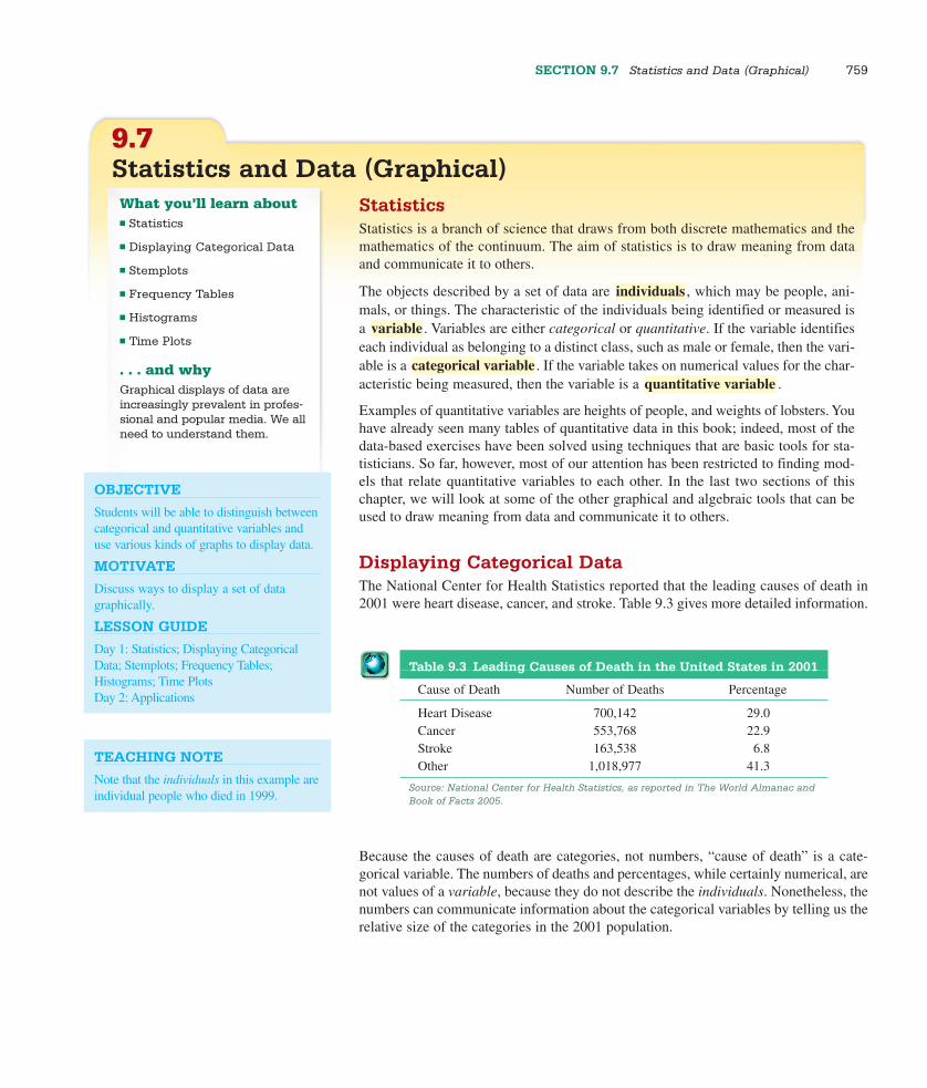
SECTION 9.7 Statistics and Data (Graphical) 759
9.7Statistics and Data (Graphical)What you’ll learn about■ Statistics
■ Displaying Categorical Data
■ Stemplots
■ Frequency Tables
■ Histograms
■ Time Plots
. . . and whyGraphical displays of data areincreasingly prevalent in profes-sional and popular media. We allneed to understand them.
OBJECTIVE
Students will be able to distinguish betweencategorical and quantitative variables anduse various kinds of graphs to display data.
MOTIVATE
Discuss ways to display a set of datagraphically.
LESSON GUIDE
Day 1: Statistics; Displaying CategoricalData; Stemplots; Frequency Tables;Histograms; Time PlotsDay 2: Applications
StatisticsStatistics is a branch of science that draws from both discrete mathematics and themathematics of the continuum. The aim of statistics is to draw meaning from dataand communicate it to others.
The objects described by a set of data are , which may be people, ani-mals, or things. The characteristic of the individuals being identified or measured isa . Variables are either categorical or quantitative. If the variable identifieseach individual as belonging to a distinct class, such as male or female, then the vari-able is a . If the variable takes on numerical values for the char-acteristic being measured, then the variable is a .
Examples of quantitative variables are heights of people, and weights of lobsters. Youhave already seen many tables of quantitative data in this book; indeed, most of thedata-based exercises have been solved using techniques that are basic tools for sta-tisticians. So far, however, most of our attention has been restricted to finding mod-els that relate quantitative variables to each other. In the last two sections of thischapter, we will look at some of the other graphical and algebraic tools that can beused to draw meaning from data and communicate it to others.
Displaying Categorical DataThe National Center for Health Statistics reported that the leading causes of death in2001 were heart disease, cancer, and stroke. Table 9.3 gives more detailed information.
quantitative variablecategorical variable
variable
individuals
Table 9.3 Leading Causes of Death in the United States in 2001
Cause of Death Number of Deaths Percentage
Heart Disease 700,142 29.0Cancer 553,768 22.9Stroke 163,538 6.8Other 1,018,977 41.3
Source: National Center for Health Statistics, as reported in The World Almanac andBook of Facts 2005.
Because the causes of death are categories, not numbers, “cause of death” is a cate-gorical variable. The numbers of deaths and percentages, while certainly numerical, arenot values of a variable, because they do not describe the individuals. Nonetheless, thenumbers can communicate information about the categorical variables by telling us therelative size of the categories in the 2001 population.
TEACHING NOTE
Note that the individuals in this example areindividual people who died in 1999.
5144_Demana_Ch09pp699-790 1/13/06 3:07 PM Page 759

760 CHAPTER 9 Discrete Mathematics
FIGURE 9.13 Causes of death in the United States in 2001 shown in (a) a bar graph, (b) a 3-D pie chart, and (c) a circle graph.
Stroke6.8%
Other41.3%
Cancer22.9%
HeartDisease29.0%
Stroke6.8%
Other41.3%
Cancer22.9%
HeartDisease29.0%
Cause of Death
HeartDisease
Cancer Stroke Other
(a)
1,000,000
1,200,000
800,000
600,000
400,000
200,000
0
Num
ber
of D
eath
s
(b) (c)
In bar charts of categorical data, the y-axis has a numerical scale, but thex-axis is labeled by category. The rectangular bars are separated by spaces to show thatno continuous numerical scale is implied. (In this respect, a bar graph differs from a his-togram, to be described later in this section.) A circle graph or a pie chart consists ofshaded or colored sections of a circle or “pie.” The central angles for the sectors are foundby multiplying the percentages by 360°. For example, the angle for the sector represent-ing cancer victims in Figure 9.13c is
22.9% • 360° � 82.4°.
It used to require time, skill, and mathematical savvy to draw data displays that wereboth visually appealing and geometrically accurate, but modern spreadsheet programshave made it possible for anyone with a computer to produce high-quality graphs fromtabular data with the click of a button.
StemplotsA quick way to organize and display a small set of quantitative data is with a ,
also called a . Each number in the data set is split into a ,
consisting of its initial digit or digits, and a , which is its final digit.leafstemstem-and-leaf plot
stemplot
We can get that information directly from the numbers, but it is very helpful to see thecomparative sizes visually. This is why you will often see categorical data displayed graph-ically, as a (Figure 9.13a), a (Figure 9.13b), or a (Figure 9.13c). For variety, the popular press also makes use of picture graphs suitedto the categories being displayed. For example, the bars in Figure 9.13a could be madeto look like tombstones of different sizes to emphasize that these are causes of death.In each case, the graph provides a visualization of the relative sizes of the categories,with the pie chart and circle graph providing the added visualization of how the cate-gories are parts of a whole population.
circle graphpie chartbar chart
5144_Demana_Ch09pp699-790 1/13/06 3:07 PM Page 760

SECTION 9.7 Statistics and Data (Graphical) 761
Stem Leaf
5 76 7 8 5 9 6 7 9
10 6 11 0 2 2 3 3 6 7 712 0 0 1 1 1 1 3 4 4 5 7 8 9 13 0 0 0 1 2 2 3 3 3 4 5 5 6 8 14 0 3 4 5 7 9 15 3 6 16 17 6
Notice that we include the “leafless” stems (6, 7, 16) in our plot, as those empty gapsare significant features of the visualization. For the same reason, be sure that each“leaf” takes up the same space along the stem. A branch with twice as many leavesshould appear to be twice as long. Now try Exercise 1.
EXAMPLE 1 Making a StemplotTable 9.4 gives the percentage of each state’s population that was 65 or older in thelast official Census (2000). Make a stemplot for the data.
SOLUTION To form the stem-and-leaf plot, we use the whole number part of each number as the stem and the tenths digit as the leaf. We write the stems in orderdown the first column and, for each number, write the leaf in the appropriate stemrow. Then we arrange the leaves in each stem row in ascending order. The final plotlooks like this:
Table 9.4 Percentages of State Residents in 2000 Who Were 65 or Older
AL 13.0 HI 13.3 MA 13.5 NM 11.7 SD 14.3AK 5.7 ID 11.3 MI 12.3 NY 12.9 TN 12.4AZ 13.0 IL 12.1 MN 12.1 NC 12.0 TX 9.9AR 14.0 IN 12.4 MS 12.1 ND 14.7 UT 8.5CA 10.6 IO 14.9 MO 13.5 OH 13.3 VT 12.7CO 9.7 KS 13.3 MT 13.4 OK 13.2 VA 11.2CT 13.8 KY 12.5 NE 13.6 OR 12.8 WA 11.2DE 13.0 LA 11.6 NV 11.0 PA 15.6 WV 15.3FL 17.6 ME 14.4 NH 12.0 RI 14.5 WI 13.1GA 9.6 MD 11.3 NJ 13.2 SC 12.1 WY 11.7
Source: U.S. Census Bureau, 2001.
5144_Demana_Ch09pp699-790 1/13/06 3:07 PM Page 761

762 CHAPTER 9 Discrete Mathematics
EXAMPLE 2 Making a Split-Stem StemplotThe per capita federal aid to state and local governments for the top 15 states (in thiscategory) in 2003 are shown in Table 9.5. Make a stemplot that provides a good visu-alization of the data. What is the average of the 15 numbers? Why is the stemplot abetter summary of the data than the average?
EXPLORATION 1 Using Information from a Stemplot
By looking at both the stemplot and the table, answer the following questionsabout the distribution of senior citizens among the 50 states.
1. Judging from the stemplot, what was the approximate average nationalpercentage of residents who were 65 or older?
2. In how many states were more than 15% of the residents 65 or older? 3
3. Which states were in the bottom tenth of all states in this statistic?
4. The numbers 5.7 and 17.6 are so far above or below the other numbers inthis stemplot that statisticians would call them outliers. Quite often there issome special circumstance that sets outliers apart from the other individu-als under study and explains the unusual data. What could explain the twooutliers in this stemplot?
EXPLORATION EXTENSIONS
Have the students discuss how the data fromTable 9.4 might have been organized in abar graph and a circle graph. Then havethem discuss the benefits of using the stem-plot for answering the questions in thisExploration.
Sometimes the data are so tightly clustered that a stemplot has too few stems to give ameaningful visualization of the data. In such cases we can spread the data out by split-ting the stems, as in Example 2.
Table 9.5 Federal Aid to State and Local GovernmentsPer Capita (2003) in Dollars
AL 3713 ND 1900 MI 1709WY 2829 ME 1836 MT 1563NY 2262 WV 1823 MA 1533NM 2005 SD 1799 KY 1449VT 1913 R1 1724 LA 1443
Source: U.S. Census Bureau Public Information Office.
SOLUTION We first round the data to $100 units, which does not affect the visu-alization. Then, to spread out the data a bit, we split each stem, putting leaves 0–4on the lower stem and leaves 5–9 on the upper stem.
Stem Leaf
1 4 41 5 6 7 7 8 8 8 9 9 2 0 32 83 3 7
continued
5144_Demana_Ch09pp699-790 1/13/06 3:07 PM Page 762

SECTION 9.7 Statistics and Data (Graphical) 763
The average of the 15 numbers is $1,967, but this is misleading. The table shows thateleven of the numbers are lower than that, while only four are higher. It is better toobserve that the distribution is clustered fairly tightly around $1,800, with the num-ber for Alabama being a significant outlier on the high end.
Now try Exercise 3.
Sometimes it is easier to compare two sets of data if we have a visualization that allowsus to view both stemplots simultaneously. use the samestems, but leaves from one set of data are added to the left, while leaves from anotherset are added to the right.
Back-to-back stem-plots
Mark McGwire Barry Bonds
9 9 3 01 6 9
9 2 2 4 5 5 9 9 3 2 2 3 3 3 4 4 7 7
9 2 4 0 2 6 98 2 5
5 60 7 3
EXAMPLE 3 Making Back-to-Back StemplotsMark McGwire and Barry Bonds entered the major leagues in 1986 and had over-lapping careers until 2001, the year that McGwire retired. During that period theyaveraged 36.44 and 35.44 home runs per year, respectively. Compare their annualhome run totals with a back-to-back stemplot. Can you tell which player was moreconsistent as a home run hitter?
SOLUTION We form a back-to-back stemplot with McGwire’s totals branchingoff to the left and Bond’s to the right.
The single-digit home run years for McGwire can be explained by fewer times at bat(late entry into the league in 1986 and injuries in 1993 and 1994). If those years areignored as anomalies, McGwire’s numbers seem to indicate more consistency. Bond’srecord-setting 73 in 2001 was (and still is) an outlier of such magnitude that it actuallyinspired more skepticism than admiration among baseball fans.
Now try Exercise 5.
Table 9.6 Major League Home Run Totals for Mark McGwire and Barry Bonds through 2001
Year 86 87 88 89 90 91 92 93 94 95 96 97 98 99 00 01
McGwire 3 49 32 33 39 22 42 9 9 39 52 58 70 65 32 29Bonds 16 25 24 19 33 25 34 46 37 33 42 40 37 34 49 73
Source: Major League Baseball Enterprises, 2002.
5144_Demana_Ch09pp699-790 1/13/06 3:07 PM Page 763
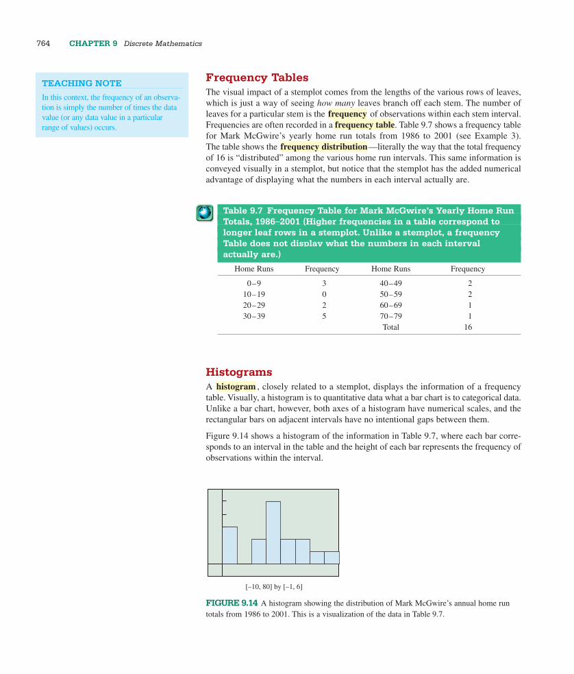
764 CHAPTER 9 Discrete Mathematics
TEACHING NOTE
In this context, the frequency of an observa-tion is simply the number of times the datavalue (or any data value in a particularrange of values) occurs.
FIGURE 9.14 A histogram showing the distribution of Mark McGwire’s annual home runtotals from 1986 to 2001. This is a visualization of the data in Table 9.7.
[–10, 80] by [–1, 6]
Frequency TablesThe visual impact of a stemplot comes from the lengths of the various rows of leaves,which is just a way of seeing how many leaves branch off each stem. The number ofleaves for a particular stem is the of observations within each stem interval.Frequencies are often recorded in a frequency table. Table 9.7 shows a frequency tablefor Mark McGwire’s yearly home run totals from 1986 to 2001 (see Example 3). The table shows the —literally the way that the total frequencyof 16 is “distributed” among the various home run intervals. This same information isconveyed visually in a stemplot, but notice that the stemplot has the added numericaladvantage of displaying what the numbers in each interval actually are.
HistogramsA , closely related to a stemplot, displays the information of a frequencytable. Visually, a histogram is to quantitative data what a bar chart is to categorical data.Unlike a bar chart, however, both axes of a histogram have numerical scales, and therectangular bars on adjacent intervals have no intentional gaps between them.
Figure 9.14 shows a histogram of the information in Table 9.7, where each bar corre-sponds to an interval in the table and the height of each bar represents the frequency ofobservations within the interval.
histogram
Table 9.7 Frequency Table for Mark McGwire’s Yearly Home RunTotals, 1986–2001 (Higher frequencies in a table correspond tolonger leaf rows in a stemplot. Unlike a stemplot, a frequency Table does not display what the numbers in each interval actually are.)
Home Runs Frequency Home Runs Frequency
0–9 3 40–49 2 10–19 0 50–59 220–29 2 60–69 1 30–39 5 70–79 1
Total 16
frequency distribution
frequency
5144_Demana_Ch09pp699-790 1/13/06 3:07 PM Page 764
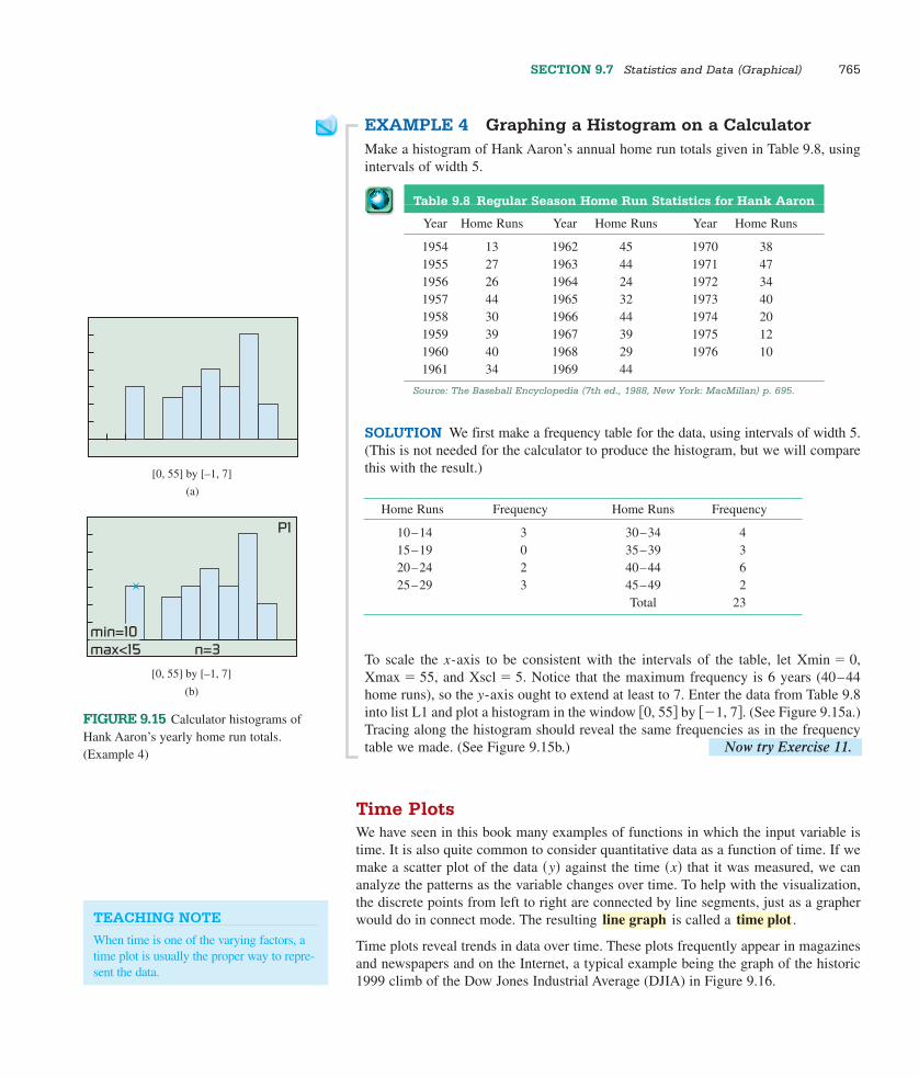
SECTION 9.7 Statistics and Data (Graphical) 765
EXAMPLE 4 Graphing a Histogram on a CalculatorMake a histogram of Hank Aaron’s annual home run totals given in Table 9.8, usingintervals of width 5.
SOLUTION We first make a frequency table for the data, using intervals of width 5.(This is not needed for the calculator to produce the histogram, but we will comparethis with the result.)
Table 9.8 Regular Season Home Run Statistics for Hank Aaron
Year Home Runs Year Home Runs Year Home Runs
1954 13 1962 45 1970 381955 27 1963 44 1971 471956 26 1964 24 1972 341957 44 1965 32 1973 401958 30 1966 44 1974 201959 39 1967 39 1975 121960 40 1968 29 1976 101961 34 1969 44
Source: The Baseball Encyclopedia (7th ed., 1988, New York: MacMillan) p. 695.
Home Runs Frequency Home Runs Frequency
10–14 3 30–34 415–19 0 35–39 320–24 2 40–44 625–29 3 45–49 2
Total 23
To scale the x-axis to be consistent with the intervals of the table, let Xmin � 0,Xmax � 55, and Xscl � 5. Notice that the maximum frequency is 6 years (40–44home runs), so the y-axis ought to extend at least to 7. Enter the data from Table 9.8into list L1 and plot a histogram in the window �0, 55� by ��1, 7�. (See Figure 9.15a.)Tracing along the histogram should reveal the same frequencies as in the frequencytable we made. (See Figure 9.15b.) Now try Exercise 11.
Time PlotsWe have seen in this book many examples of functions in which the input variable istime. It is also quite common to consider quantitative data as a function of time. If wemake a scatter plot of the data �y� against the time �x� that it was measured, we cananalyze the patterns as the variable changes over time. To help with the visualization,the discrete points from left to right are connected by line segments, just as a grapherwould do in connect mode. The resulting is called a .
Time plots reveal trends in data over time. These plots frequently appear in magazinesand newspapers and on the Internet, a typical example being the graph of the historic1999 climb of the Dow Jones Industrial Average (DJIA) in Figure 9.16.
time plotline graph
FIGURE 9.15 Calculator histograms ofHank Aaron’s yearly home run totals.(Example 4)
[0, 55] by [–1, 7]
(b)
[0, 55] by [–1, 7]
(a)
P1
n=3min=10max<15
TEACHING NOTE
When time is one of the varying factors, atime plot is usually the proper way to repre-sent the data.
5144_Demana_Ch09pp699-790 1/13/06 3:07 PM Page 765

766 CHAPTER 9 Discrete Mathematics
FIGURE 9.16 Time plot of the Dow Jones Industrial Average during the spectacular year 1999. Investors get a good visu-alization of where the stock market has been, although the trick is to figure out where it is going. (Source: Quote.com, asreported by the Associated Press in the Chattanooga Times/Free Press.)
March 29,1999First closeabove 10,000
Dec. 31 19989181.43
Nov. 16Fed raisesinterest rates
Dec. 2311,405.76+24.23%
Aug. 24Fed raisesinterest rates
June 30Fed raisesinterest rates
Daily closesJ JJA AM MF S O N D
9,000
9,500
10,000
10,500
11,000
11,500
Table 9.9 Millions of Units of CDs Shipped to Retailers Each Year 1991–2003
Year 1991 1992 1993 1994 1995 1996 1997 1998 1999 2000 2001 2002 2003
CDs 333.3 407.5 495.4 662.1 722.9 778.9 753.1 847.0 938.9 942.5 881.9 803.3 745.9
Source: Recording Industry Association of America, as reported in the World Almanac and Book of Facts 2005.
FIGURE 9.17 A time plot of CD volumeover the years from 1991 to 2003, as reflectedin shipments to retailers. (Example 5)
1991 2003
100
1000
y
x
EXAMPLE 5 Drawing a Time PlotTable 9.9 gives the number of compact disc (CD) units shipped to retailers each yearin the 13-year period from 1991 to 2003. (The numbers are shown in millions, netafter returns.) Display the data in a time plot and analyze the 13-year trend.
SOLUTION The horizontal axis represents time (in years) from 1991 to 2003. Thevertical axis represents the number of CDs shipped that year, in millions of units.Since the visualization is enhanced by showing both axes in the viewing window, thevertical axis of a time plot is usually translated to cross the x-axis at or near the begin-ning of the time interval in the data. You can create this effect on your grapher byentering the years as �1, 2, 3, . . . , 13� rather than �1991, 1992, 1993, . . . , 2003�. Thelabeling on the x-axis can then display the years, as shown in Figure 9.17.
The time plot shows that CD shipments increased steadily from 1991 to 1999 withespecially good years from 1994 to 1996; then they declined steadily from 2000 to2003. The music industry knew the reason for the dramatic turnaround—do you?
Now try Exercise 17.
5144_Demana_Ch09pp699-790 1/13/06 3:07 PM Page 766

SECTION 9.7 Statistics and Data (Graphical) 767
FOLLOW-UP
Discuss ways to determine whether a barchart, circle graph, stemplot, histogram, ortime plot would be the most effective wayto display a set of data.
ASSIGNMENT GUIDE
Day 1: Ex. 2–10 even, 16–20Day 2: Ex. 23–25, 27–32, 35, 36
COOPERATIVE LEARNING
Group Activity: Ex. 33, 34
NOTES ON EXERCISES
Most of the exercises in this section are rou-tine and give students practice in the meth-ods of plotting data.Ex. 27–32 provide practice for standardizedtests.
ONGOING ASSESSMENT
Self-Assessment: Ex. 1, 3, 5, 11, 17, 19Embedded Assessment: Ex. 20, 23, 24
Table 9.10 Millions of Units of Cassettes Shipped to Retailers, 1991–2003
Year 1991 1992 1993 1994 1995 1996 1997 1998 1999 2000 2001 2002 2003
Cass 360.1 366.4 339.5 345.4 272.6 225.3 172.6 158.5 123.6 76 45 31.1 17.2
Source: Recording Industry Association of America, as reported in the World Almanac and Book of Facts 2005.
FIGURE 9.18 A time plot comparing cassette shipments and CD shipments for the time periodfrom 1991 to 2003. (Example 6)
1991 2003
100
500
1000
EXAMPLE 6 Overlaying Two Time PlotsTable 9.10 gives the number of cassette units shipped to retailers each year in the 13-year period from 1991 to 2003. (The numbers are shown in millions, net afterreturns.) Compare the cassette trend with the CD trend by overlaying the time plotsfor the two products.
SOLUTION The two time plots are shown in Figure 9.18. The popularity of cas-sette tapes declined as more consumers switched to CD (and eventually MP3)technology. Now try Exercise 19.
QUICK REVIEW 9.7In Exercises 1–6, solve for the required value.
1. 457 is what percent of 2953? � 15.48%
2. 827 is what percent of 3950? � 20.94%
3. 52° is what percent of 360°? � 14.44%
4. 98° is what percent of 360°? � 27.22%
5. 734 is 42.6% of what number? � 1723
6. 5106 is 55.5% of what number? 9200
In Exercises 7–10, round the given value to the nearest whole num-ber in the specified units.
7. $234,598.43 (thousands of dollars) $235 thousand
8. 237,834,289 (millions) 238 million
9. 848.36 thousands (millions) 1 million
10. 1432 millions (billions) 1 billion
5144_Demana_Ch09pp699-790 1/13/06 3:07 PM Page 767

768 CHAPTER 9 Discrete Mathematics
SECTION 9.7 EXERCISES
Table 9.11 shows the home run statistics for Roger Maris during hismajor league career.
1. Make a stemplot of the data in Table 9.11. Are there any outliers?
2. Make a back-to-back stemplot comparing the annual home runproduction of Roger Maris (Table 9.11) with that of Hank Aaron(Table 9.8 on page 765). Write a brief interpretation of the stemplot.
In Exercises 3–6, construct the indicated stemplot from the data inTable 9.12. Then write a brief interpretation of the stemplot.
3. A stemplot showing life expectancies of males in the nations ofSouth America (Round to nearest year and use split stems.)
4. A stemplot showing life expectancies of females in the nations ofSouth America (Round to nearest year and use split stems.)
5. A back-to-back stemplot for life expectancies of males andfemales in the nations of South America (Round to nearest yearand use split stems.)
6. A stemplot showing the difference between female and male lifeexpectancies in the nations of South America (Use unrounded dataand do not split stems.)
In Exercises 7 and 8, use the data in Table 9.12 to construct the indicatedfrequency table, using intervals 60.0–64.9, 65.0–69.9, etc.
7. Life expectancies of males in the nations of South America
8. Life expectancies of females in the nations of South America
In Exercises 9–12, draw a histogram for the given table.
9. The frequency table in Exercise 7
10. The frequency table in Exercise 8
11. Table 9.13 of Willie Mays’ annual home run totals, using intervals1–5, 6–10, 11–15, etc.
12. Table 9.13 of Mickey Mantle’s annual home run totals, using inter-vals 0–4, 5–9, 10–14, etc.
In Exercises 13–16, make a time plot for the indicated data.
13. Willie Mays’s annual home run totals given in Table 9.13
14. Mickey Mantle’s annual home run totals given in Table 9.13
15. Mark McGwire’s home run totals given in Table 9.6 on page 763
16. Hank Aaron’s home run totals given in Table 9.8 on page 765
Table 9.13 Regular Season Home Run Statistics for Willie Mays and Mickey Mantle
Year Mays Mantle Year Mays Mantle
1951 20 13 1962 38 301952 4 23 1963 47 151953 41 21 1964 52 351954 51 27 1965 37 191955 36 37 1966 22 231956 35 52 1967 23 221957 29 34 1968 13 181958 34 42 1969 281959 29 31 1970 181960 40 40 1971 81961 49 54 1972 6
Source: The Baseball Encyclopedia, 7th ed., 1988.
Table 9.12 Life Expectancy by Gender for the Nations of South America
Nation Male Female
Argentina 72.0 79.7Bolivia 62.5 67.9Brazil 67.5 75.6Chile 73.1 79.8Colombia 67.6 75.4Ecuador 73.2 79.0Guyana 60.1 64.8Paraguay 72.1 77.3Peru 67.5 71.0Suriname 66.8 71.6Uruguay 72.7 79.2Venezuela 71.0 77.3
Source: The World Almanac and Book of Facts, 2005.
Table 9.11 Regular Season Home RunStatistics for Roger Maris
Year Home Runs
1957 141958 281959 161960 391961 611962 331963 231964 261965 81966 131967 91968 5
Source: The Baseball Encyclopedia, 7th ed., 1988.
5144_Demana_Ch09pp699-790 1/13/06 3:07 PM Page 768

SECTION 9.7 Statistics and Data (Graphical) 769
Table 9.14 shows the total amount of money won (in units of $1000,rounded to the nearest whole number) by the leading money winnersin women’s (LPGA) and men’s (PGA) professional golf for selectedyears between 1970 and 2003.
17. Make a time plot for the men’s winnings in Table 9.14. Write abrief interpretation of the time plot.
18. Make a time plot for the women’s winnings in Table 9.14. Write abrief interpretation of the time plot.
19. Compare the trends in Table 9.14 by overlaying the time plots.Write a brief interpretation.
20. Writing to Learn (Continuation of Exercise 19)The data in Table 9.14 show that the earnings for the top PGA player rose by a modest 68% in the decade from 1975 to 1985, while the earningsfor the top LPGA player rose by a whopping 338%.Although this was, in fact, a strong growth periodfor women’s sports, statisticians would be unlikelyto draw any conclusions from a comparison of thesetwo numbers. Use the visualization from the com-parative time plot in Exercise 19 to explain why.
In Exercises 21 and 22, compare performances by overlaying timeplots.
21. The time plots from Exercises 13 and 14 to compare the perfor-mances of Mays and Mantle
22. The time plots from Exercises 15 and 16 to compare the perfor-mances of McGwire and Aaron
Table 9.14 Yearly Winnings (in Thousands of Dollars) of the Top Money Winners in Men’s and Women’s Golf for Selected Years 1970–2003
Year Men (PGA) Women (LPGA)
1970 157 301975 323 951980 531 2311985 542 4161990 1165 8641995 1655 6671996 1780 10021997 2067 12371998 2591 10931999 6617 15922000 9188 18772001 5688 21062002 6913 28642003 7574 2030
Source: The World Almanac and Book of Facts 2005.
In Exercises 23 and 24, analyze the data as indicated.
23. The salaries of the workers in one department of the GarciaBrothers Company (given in thousands of dollars) are as follows:
33.5, 35.3, 33.8, 29.3, 36.7, 32.8, 31.7, 36.3, 33.5, 28.2, 34.8,33.5, 35.3, 29.7, 38.5, 32.7, 34.8, 34.2, 31.6, 35.4
(a) Complete a stemplot for this data set.
(b) Create a frequency table for the data.
(c) Draw a histogram for the data. What viewing window didyou use?
(d) Why does a time plot not work well for the data?
24. The average wind speeds for one year at 44 climatic data centersaround the United States are as follows:
9.0, 6.9, 9.1, 9.2, 10.2, 12.5, 12.0, 11.2, 12.9, 10.3, 10.6, 10.9, 8.7,10.3, 11.0, 7.7, 11.4, 7.9, 9.6, 8.0, 10.7, 9.3, 7.9, 6.2, 8.3, 8.9, 9.3,11.6, 10.6, 9.0, 8.2, 9.4, 10.6, 9.5, 6.3, 9.1, 7.9, 9.7, 8.8, 6.9, 8.7,9.0, 8.9, 9.3
(a) Complete a stemplot for this data set.
(b) Create a frequency table for the data.
(c) Draw a histogram for the data. What viewing window didyou use?
(d) Why does a circle graph not work well for the data?
In Exercises 25 and 26, compare by overlaying time plots for the datain Table 9.15
25. The populations of California, New York, and Texas from 1990through 2000
26. The populations of Florida, Illinois, and Pennsylvania from 1990through 2000
Table 9.15 Population (in millions) ofthe Six Most Populous States
Census CA FL IL NY PA TX
1900 1.5 0.5 4.8 7.3 6.3 3.01910 2.4 0.8 5.6 9.1 7.7 3.91920 3.4 1.0 6.5 10.4 8.7 4.71930 5.7 1.5 7.6 12.6 9.6 5.81940 6.9 1.9 7.9 13.5 9.9 6.41950 10.6 2.8 8.7 14.8 10.5 7.71960 15.7 5.0 10.1 16.8 11.3 9.61970 20.0 6.8 11.1 18.2 11.8 11.21980 23.7 9.7 11.4 17.6 11.9 14.21990 29.8 12.9 11.4 18.0 11.9 17.02000 33.9 16.0 12.4 19.0 12.3 20.9
Source: The World Almanac and Book of Facts 2005.
5144_Demana_Ch09pp699-790 1/13/06 3:07 PM Page 769
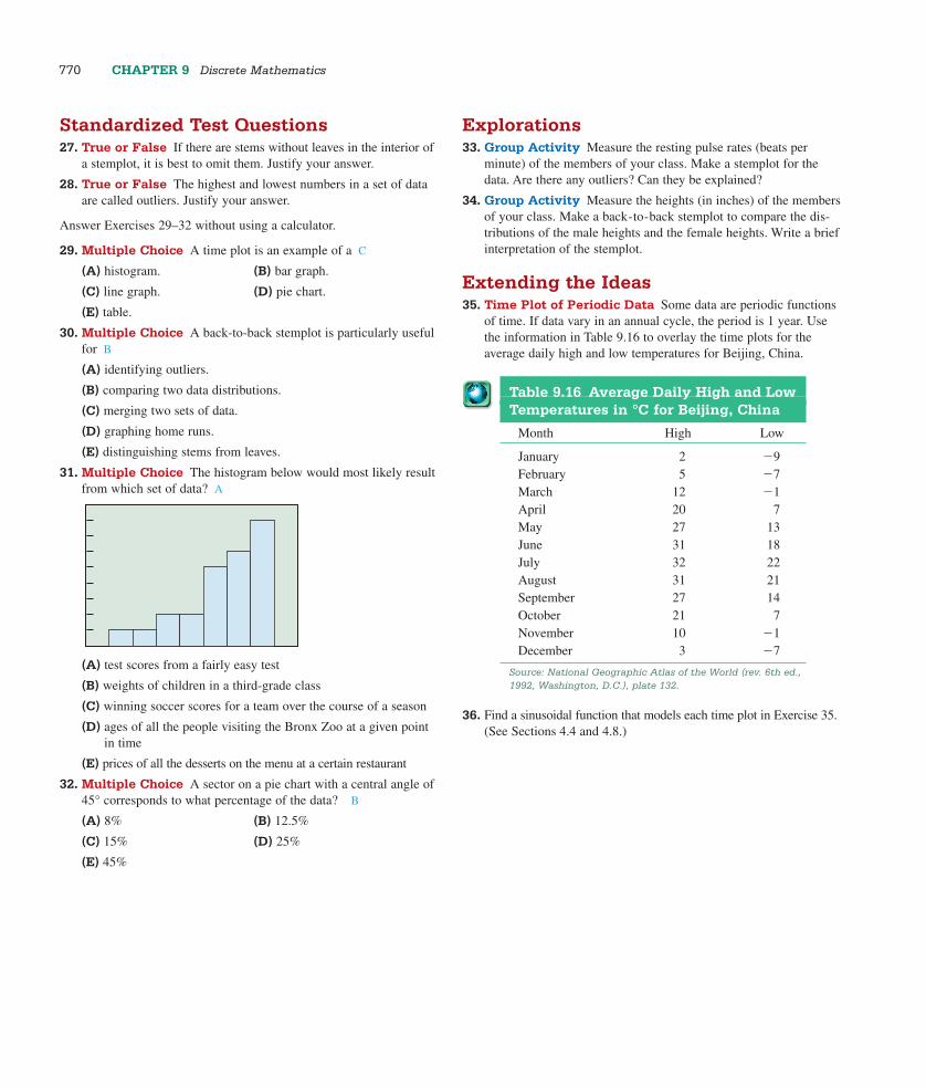
770 CHAPTER 9 Discrete Mathematics
Standardized Test Questions27. True or False If there are stems without leaves in the interior of
a stemplot, it is best to omit them. Justify your answer.
28. True or False The highest and lowest numbers in a set of dataare called outliers. Justify your answer.
Answer Exercises 29–32 without using a calculator.
29. Multiple Choice A time plot is an example of a C
(A) histogram. (B) bar graph.
(C) line graph. (D) pie chart.
(E) table.
30. Multiple Choice A back-to-back stemplot is particularly usefulfor B
(A) identifying outliers.
(B) comparing two data distributions.
(C) merging two sets of data.
(D) graphing home runs.
(E) distinguishing stems from leaves.
31. Multiple Choice The histogram below would most likely resultfrom which set of data? A
(A) test scores from a fairly easy test
(B) weights of children in a third-grade class
(C) winning soccer scores for a team over the course of a season
(D) ages of all the people visiting the Bronx Zoo at a given pointin time
(E) prices of all the desserts on the menu at a certain restaurant
32. Multiple Choice A sector on a pie chart with a central angle of45° corresponds to what percentage of the data? B
(A) 8% (B) 12.5%
(C) 15% (D) 25%
(E) 45%
Explorations33. Group Activity Measure the resting pulse rates (beats per
minute) of the members of your class. Make a stemplot for thedata. Are there any outliers? Can they be explained?
34. Group Activity Measure the heights (in inches) of the membersof your class. Make a back-to-back stemplot to compare the dis-tributions of the male heights and the female heights. Write a briefinterpretation of the stemplot.
Extending the Ideas35. Time Plot of Periodic Data Some data are periodic functions
of time. If data vary in an annual cycle, the period is 1 year. Usethe information in Table 9.16 to overlay the time plots for theaverage daily high and low temperatures for Beijing, China.
36. Find a sinusoidal function that models each time plot in Exercise 35.(See Sections 4.4 and 4.8.)
Table 9.16 Average Daily High and LowTemperatures in °C for Beijing, China
Month High Low
January 2 �9February 5 �7March 12 �1April 20 7May 27 13June 31 18July 32 22August 31 21September 27 14October 21 7November 10 �1December 3 �7
Source: National Geographic Atlas of the World (rev. 6th ed.,1992, Washington, D.C.), plate 132.
5144_Demana_Ch09pp699-790 1/13/06 3:07 PM Page 770

SECTION 9.8 Statistics and Data (Algebraic) 771
9.8Statistics and Data (Algebraic)What you’ll learn about■ Parameters and Statistics
■ Mean, Median, and Mode
■ The Five-Number Summary
■ Boxplots
■ Variance and StandardDeviation
■ Normal Distributions
. . . and whyThe language of statistics isbecoming more commonplacein our everyday world.
Parameters and StatisticsThe various numbers that are associated with a data set are called . Theyserve to describe the individuals from which the data come, so the gathering and pro-cessing of such numerical information is often called .You sawmany examples of descriptive statistics in Section 9.7.
The science of statistics comes in when we use descriptive statistics (like the resultsof a study of 1500 smokers) to make judgments, called inferences, about entire pop-ulations (like all smokers). Statisticians are really interested in the numbers called
that are associated with entire populations. Since it is usually eitherimpractical or impossible to measure entire populations, statisticians gather statisticsfrom carefully chosen , then use the science of tomake inferences about the parameters.
inferential statisticssamples
parameters
descriptive statistics
statistics
OBJECTIVE
Students will be able to use measures ofcenter, the five-number summary, a boxplot,standard deviation, and normal distributionto describe quantitative data.
MOTIVATE
Discuss ways to use a number to describe aset of quantitative data.
LESSON GUIDE
Day 1: Parameters and Statistics; Mean,Median, and Mode; The Five-NumberSummary; BoxplotsDay 2: Variance and Standard Deviation;Normal Distributions
TEACHING NOTE
Most students should be familar with themean, median, and mode from previousmathematics courses.
EXAMPLE 1 Distinguishing a Parameter from a StatisticA 1996 study called Kids These Days: What Americans Really Think About the NextGeneration reported that 33% of adolescents say there is no adult at home when theyreturn from school. The report was based on a survey of 600 randomly selected peo-ple aged 12 to 17 years old and had a margin of error of �4% (Source: PublicAgenda). Did the survey measure a parameter or a statistic, and what does that“margin of error” mean?
SOLUTION The survey did not measure all adolescents in the population, so it didnot measure a parameter. They sampled 600 adolescents and found a statistic. On theother hand, the statement “33% of adolescents say there is no adult at home” is mak-ing an inference about all American adolescents. We should interpret that statement interms of the margin of error, as meaning “between 29% and 37% of all American ado-lescents would say that there is no adult at home when they return from school.” In otherwords, the statisticians are confident that the parameter is within �4% of their samplestatistic, even though they only sampled 600 adolescents—a tiny fraction of the ado-lescent population! The mathematics that gives them that confidence is based on thelaws of probability and is scientifically reliable, but we will not go into it here.
Now try Exercise 1.
Mean, Median, and ModeIf you wanted to study the effect of chicken feed additives on the thickness of eggshells, you would need to sample many eggs from different hens under various feed-ing conditions. Suppose you were to gather data from 50 eggs from hens eating feedA and 50 eggs from hens eating feed B. How would you compare the two? The sim-plest way would be to find the average egg shell thickness for each feed and comparethose two numbers.
5144_Demana_Ch09pp699-790 1/13/06 3:07 PM Page 771

The word “average,” however, can have several different meanings, all of them some-how measures of center.
• If we say, “The average on last week’s test was 83.4,” we are referring to the. (This is what most people usually think of as “average.”)
• If we say, “The average test score puts you right in the middle of the class,” we arereferring to the .
• If we say, “The average American student starts college at age 18,” we are referringto the .
We will look at each of these measures separately.
mode
median
mean
772 CHAPTER 9 Discrete Mathematics
DEFINITION Mean
The of a list of n numbers �x1, x2, . . . , xn � is
x� �x1 � x2 �
n
. . . � xn� 1n
n
i�1xi.
mean
The mean is also called the arithmetic mean, arithmetic average, or average value.
EXAMPLE 2 Computing a MeanFind the mean annual home run total for Roger Maris’s major league career, 1957–1968(Table 9.11 on page 768).
SOLUTION According to Table 9.11, we are looking for the mean of thefollowing list of 12 numbers: �14, 28, 16, 39, 61, 33, 23, 26, 8, 13, 9, 5�.
x� � � 21725
� 22.9
Now try Exercise 9.
14 � 28 � 16 � � � � � 9 � 5
12
As common as it is to use the mean as a measure of center, sometimes it can be mis-leading. For example, if you were to find the mean annual salary of a Geography majorfrom the University of North Carolina working in Chicago in 1997, it would probablybe a number in the millions of dollars. This is because the group being measured,which is not very large, includes an outlier named Michael Jordan. The mean can bestrongly affected by outliers.
We call a statistic if it is not strongly affected by outliers (See Exploration 1,Section 9.7). While the mean is not a resistant measure of center, the median is.
resistant
DEFINITION Median
The of a list of n numbers �x1, x2, . . . , xn � arranged in order (eitherascending or descending) is
• the middle number if n is odd, and
• the mean of the two middle numbers if n is even.
median
5144_Demana_Ch09pp699-790 1/13/06 3:07 PM Page 772

SECTION 9.8 Statistics and Data (Algebraic) 773
À LA MODE
The mode can also be used for categoricalvariables.
Both the mean and the median are important measures of center. A somewhat lessimportant measure of center (but a measure of possible significance statistically) is themode.
EXAMPLE 3 Finding a MedianFind the median of Roger Maris’s annual home run totals. (See Example 2.)
SOLUTION First, we arrange the list in ascending order: �5, 8, 9, 13, 14, 16, 23, 26,28, 33, 39, 61�. Since there are 12 numbers, the median is the mean of the 6th and 7thnumbers:
16 �
223
� 19.5.
Notice that this number is quite a bit smaller than the mean (22.9). The mean is stronglyaffected by the outlier representing Maris’s record-breaking season, while the medianis not. The median would still have been 19.5 if he had hit only 41 home runs that sea-son, or, indeed, if he had hit 81. Now try Exercise 11.
DEFINITION Mode
The of a list of numbers is the number that appears most frequentlyin the list.
mode
EXAMPLE 4 Finding a ModeFind the mode for the annual home run totals of Hank Aaron (Table 9.8 on page 765).Is this number of any significance?
SOLUTION It helps to arrange the list in ascending order: �10, 12, 13, 20, 24, 26,27, 29, 30, 32, 34, 34, 38, 39, 39, 40, 40, 44, 44, 44, 44, 45, 47�.
Most numbers in the list appear only once. Three numbers appear twice, and the num-ber 44 appears four times. The mode is 44.
It is rather unusual to have that many repeats of a number in a list of this sort. (Bycomparison, the Maris list has no repeats—and hence no mode—while the lists forMays, Mantle, McGwire, and Bonds contain no number more than twice.) The modein this case has special significance only to baseball trivia buffs, who recognize 44 asAaron’s uniform number!
Now try Exercise 17.
NOTES ON EXAMPLES
Example 4 mentions a situation in whichthe mode does not exist.
Example 4 demonstrates why the mode is less useful as a measure of center. Themode (44) is a long way from the median (34) and the mean (32.83), either of whichdoes a much better job of representing Aaron’s annual home run output over thecourse of his career.
5144_Demana_Ch09pp699-790 1/13/06 3:07 PM Page 773

774 CHAPTER 9 Discrete Mathematics
EXAMPLE 6 Working with a Weighted Mean
At Marty’s school, it is an administrative policy that the final exam must count 25%of the semester grade. If Marty has an 88.5 average going into the final exam, whatis the minimum exam score needed to earn a 90 for the semester?
EXAMPLE 5 Using a Frequency TableA teacher gives a 10-point quiz and records the scores in a frequency table (Table 9.17)as shown below. Find the mode, median, and mean of the data.
SOLUTION The total of the frequencies is 30, so there are 30 scores.
The mode is 7, since that is the score with the highest frequency.
The median of 30 numbers will be the mean of the 15th and 16th numbers. The tableis already arranged in descending order, so we count the frequencies from left to rightuntil we come to 15. We see that the 15th number is a 7 and the 16th number is a 6.The median, therefore, is 6.5.
To find the mean, we multiply each number by its frequency, add the products, anddivide the total by 30:
Table 9.17 Quiz Scores for Example 5
Score 10 9 8 7 6 5 4 3 2 1 0Frequency 2 2 3 8 4 3 3 2 1 1 1
The formula for finding the mean of a list of numbers �x1, x2, . . . , xn� with frequencies� f1, f2, . . . , fn� is
x� � � .
This same formula can be used to find a , in which numbers �x1, x2, . . . , xn�are given before the mean is computed. The weights act the same way as fre-quencies.
weightsweighted mean
xi fi fi
x1 f1 � x2 f2 � � � � � xn fnf1 � f2 � � � � � fn
x� �
30
� 5.93�
[10�2� � 9�2� � 8�3� � 7�8� � 6�4� � 5�3�� 4�3� � 3�2� � 2�1� � 1�1� � 0�1�]
Now try Exercise 19.
TEACHING NOTE
Note that the weights used can be the val-ues 25 and 75 or 0.25 and 0.75. Eithermethod will give the same result for theaverage value.
continued
5144_Demana_Ch09pp699-790 1/13/06 3:07 PM Page 774

SECTION 9.8 Statistics and Data (Algebraic) 775
ALERT
Stress the difference between the range of afunction (which is a set of numbers) and therange of a data set (which is a number).
The Five-Number SummaryMeasures of center tell only part of the story of a data set. They do not indicate howwidely distributed or highly variable the data are. Measures of spread do. The simplestand crudest measure of spread is the , which is the difference between the max-imum and minimum values in the data set:
Range � maximum � minimum.
For example, the range of numbers in Roger Maris’s annual home run production is61 � 5 � 56. Like the mean, the range is a statistic that is strongly influenced by out-liers, so it can be misleading. A more resistant (and therefore more useful) measure isthe interquartile range, which is the range of the middle half of the data.
Just as the median separates the data into halves, the separate the data intofourths. The Q1 is the median of the lower half of the data, the
is the median, and the Q3 is the median of the upperhalf of the data. The (IQR) measures the spread between the firstand third quartiles, comprising the middle half of the data:
IQR � Q3 � Q1.
Taken together, the maximum, the minimum, and the three quartiles give a fairly com-plete picture of both the center and the spread of a data set.
interquartile rangethird quartilesecond quartile
first quartilequartiles
range
SOLUTION The preliminary average (88.5) is given a weight of 0.75 and the finalexam (x) is given a weight of 0.25. We will assume that a semester average of 89.5will be rounded to a 90 on the transcript. Therefore,
� 89.5
0.25x � 89.5�1� � 88.5�0.75�
x � 92.5
Interpreting the answer, we conclude that Marty needs to make a 93 on the final exam.
Now try Exercise 21.
88.5�0.75� � x�0.25�
0.75 � 0.25
FINDING QUARTILES
When we are finding the quartiles for adata set with an odd number of values,we do not consider the middle value to beincluded in either the lower or the upperhalf of the data.
DEFINITION Five-Number Summary
The of a data set is the collection
�minimum, Q1, median, Q3, maximum�.
five-number summary
COMPUTING STATISTICS
ON A CALCULATOR
Modern calculators will usually processlists of data and give statistics like themean, median, and quartiles with a pushof a button. Consult your owner’s manual.
EXAMPLE 7 Five-Number Summary and SpreadFind the five-number summaries for the male and female life expectancies in SouthAmerican nations (Table 9.12 on page 768) and compare the spreads.
SOLUTION Here are the lists in ascending order.
Males:
�59.0, 60.5, 61.5, 66.7, 67.9, 68.5, 69.0, 70.3, 71.4, 71.9, 72.1, 72.6�continued
5144_Demana_Ch09pp699-790 1/13/06 3:07 PM Page 775

776 CHAPTER 9 Discrete Mathematics
You can learn a lot about the data by considering the shape of the distribution, as visu-alized in a histogram. Try answering the questions in Exploration 1.
Females:
�66.2, 66.7, 67.7, 72.8, 74.3, 74.4, 74.6, 76.5, 76.6, 78.8, 79.0, 79.4�
We have spaced the lists to show where the quartiles appear. The median of the 12values is midway between the 6th and 7th values. The first quartile is the median ofthe lower 6 values (i.e., midway between the 3rd and 4th), and the third quartile is themedian of the upper 6 values (i.e., midway between the 9th and 10th).
The five-number summaries are shown below.
Males: �59.0, 64.1, 68.75, 71.65, 72.6�
Females: �66.2, 70.25, 74.5, 77.7, 79.4�
The males have a range of 72.6 � 59.0 � 13.6 and an IQR of 71.65 � 64.1 � 7.55.
The females have a range of 79.4 � 66.2 � 13.2 and an IQR of 77.7 � 70.25 � 7.45.
Not only do the women live longer, but there is less variability in their life expectan-cies (as measured by the IQR). Male life expectancy is more strongly affected by dif-ferent political conditions within countries (war, civil strife, crime, etc.).
Now try Exercise 23.
EXPLORATION 1 Interpreting Histograms
1. Of the two histograms shown in Figure 9.19, which displays a data set withmore variability? Figure (b)
2. Of the three histograms in Figure 9.20, which has a median less than itsmean? Which has a median greater than its mean? Which has a medianapproximately equal to its mean? Figure (b); Figure (c); Figure (a)
EXPLORATION EXTENSIONS
Have the students discuss which might bethe better statistic to use (mean or median)for interpreting the data in the graphs ofFigure 9.20.
FIGURE 9.19 Which data set has morevariability? (Exploration 1)
(b)
(a)
FIGURE 9.20 Which graph shows a data set in which the mean is less than the median? Greater than the median? Approximatelyequal to the median? (Exploration 1)
(a) (b) (c)
5144_Demana_Ch09pp699-790 1/13/06 3:07 PM Page 776
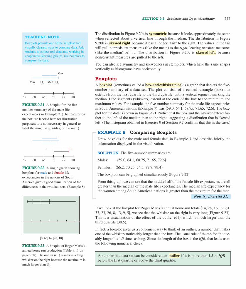
SECTION 9.8 Statistics and Data (Algebraic) 777
TEACHING NOTE
Boxplots provide one of the simplest andvisually clearest ways to compare data. Askstudents to collect real data and, working incooperative learning groups, use boxplots tocompare the data.
FIGURE 9.21 A boxplot for the five-number summary of the male lifeexpectancies in Example 7. (The features onthe box are labeled here for illustrativepurposes; it is not necessary in general tolabel the min, the quartiles, or the max.)
Min
Max
Med Q3
Q1
7570656055 80
FIGURE 9.22 A single graph showingboxplots for male and female lifeexpectancies in the nations of SouthAmerica gives a good visualization of thedifferences in the two data sets. (Example 8)
7570656055 80
The distribution in Figure 9.20a is because it looks approximately the samewhen reflected about a vertical line through the median. The distribution in Figure9.20b is because it has a longer “tail” to the right. The values in the tailwill pull nonresistant measures (like the mean) to the right, leaving resistant measures(like the median) behind. The distribution in Figure 9.20c is becausenonresistant measures are pulled to the left.
You can also see symmetry and skewedness in stemplots, which have the same shapesvertically as histograms have horizontally.
BoxplotsA (sometimes called a ) is a graph that depicts the five-number summary of a data set. The plot consists of a central rectangle (box) thatextends from the first quartile to the third quartile, with a vertical segment marking themedian. Line segments (whiskers) extend at the ends of the box to the minimum andmaximum values. For example, the five-number summary for the male life expectanciesin South American nations (Example 7) was �59.0, 64.1, 68.75, 71.65, 72.6�. The box-plot for the data is shown in Figure 9.21. Notice that the box and the whisker extend fur-ther to the left of the median than to the right, suggesting a distribution that is skewedleft. (The histogram obtained in Exercise 9 of Section 9.7 confirms that this is the case.)
EXAMPLE 8 Comparing BoxplotsDraw boxplots for the male and female data in Example 7 and describe briefly theinformation displayed in the visualization.
SOLUTION The five-number summaries are:
Males: �59.0, 64.1, 68.75, 71.65, 72.6�
Females: �66.2, 70.25, 74.5, 77.7, 79.4�
The boxplots can be graphed simultaneously (Figure 9.22).
From this graph we can see that the middle half of the female life expectancies are allgreater than the median of the male life expectancies. The median life expectancy forthe women among South American nations is greater than the maximum for the men.
Now try Exercise 31.
box-and-whisker plotboxplot
skewed left,
skewed right
symmetric
If we look at the boxplot for Roger Maris’s annual home run totals �14, 28, 16, 39, 61,33, 23, 26, 8, 13, 9, 5�, we see that the whisker on the right is very long (Figure 9.23).This is a visualization of the effect of the outlier (61), which is much larger than thethird quartile (30.5).
In fact, a boxplot gives us a convenient way to think of an outlier: a number that makesone of the whiskers noticeably longer than the box. The usual rule of thumb for “notice-ably longer” is 1.5 times as long. Since the length of the box is the IQR, that leads us tothe following numerical check.
A number in a data set can be considered an if it is more than 1.5 � IQRbelow the first quartile or above the third quartile.
outlier
FIGURE 9.23 A boxplot of Roger Maris’sannual home run production (Table 9.11 onpage 768). The outlier (61) results in a longwhisker on the right because the maximum ismuch larger than Q3.
[0, 65] by [–5, 10]
5144_Demana_Ch09pp699-790 1/13/06 3:07 PM Page 777
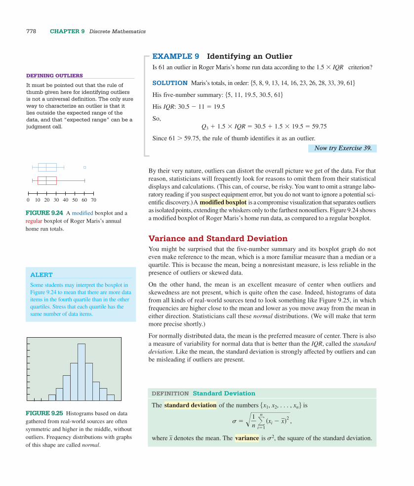
778 CHAPTER 9 Discrete Mathematics
DEFINING OUTLIERS
It must be pointed out that the rule ofthumb given here for identifying outliersis not a universal definition. The only sureway to characterize an outlier is that itlies outside the expected range of thedata, and that “expected range” can be ajudgment call.
EXAMPLE 9 Identifying an OutlierIs 61 an outlier in Roger Maris’s home run data according to the 1.5 � IQR criterion?
SOLUTION Maris’s totals, in order: �5, 8, 9, 13, 14, 16, 23, 26, 28, 33, 39, 61�
His five-number summary: �5, 11, 19.5, 30.5, 61�
His IQR: 30.5 � 11 � 19.5
So,Q3 � 1.5 � IQR � 30.5 � 1.5 � 19.5 � 59.75
Since 61 � 59.75, the rule of thumb identifies it as an outlier.
Now try Exercise 39.
By their very nature, outliers can distort the overall picture we get of the data. For thatreason, statisticians will frequently look for reasons to omit them from their statisticaldisplays and calculations. (This can, of course, be risky. You want to omit a strange labo-ratory reading if you suspect equipment error, but you do not want to ignore a potential sci-entific discovery.)A is a compromise visualization that separates outliersas isolated points, extending the whiskers only to the farthest nonoutliers. Figure 9.24 showsa modified boxplot of Roger Maris’s home run data, as compared to a regular boxplot.
Variance and Standard DeviationYou might be surprised that the five-number summary and its boxplot graph do noteven make reference to the mean, which is a more familiar measure than a median or aquartile. This is because the mean, being a nonresistant measure, is less reliable in thepresence of outliers or skewed data.
On the other hand, the mean is an excellent measure of center when outliers andskewedness are not present, which is quite often the case. Indeed, histograms of datafrom all kinds of real-world sources tend to look something like Figure 9.25, in whichfrequencies are higher close to the mean and lower as you move away from the mean ineither direction. Statisticians call these normal distributions. (We will make that termmore precise shortly.)
For normally distributed data, the mean is the preferred measure of center. There is alsoa measure of variability for normal data that is better than the IQR, called the standarddeviation. Like the mean, the standard deviation is strongly affected by outliers and canbe misleading if outliers are present.
modified boxplot
FIGURE 9.24 A modified boxplot and aregular boxplot of Roger Maris’s annualhome run totals.
403020100 50 60 70
ALERT
Some students may interpret the boxplot inFigure 9.24 to mean that there are more dataitems in the fourth quartile than in the otherquartiles. Stress that each quartile has thesame number of data items.
DEFINITION Standard Deviation
The of the numbers �x1, x2, . . . , xn � is
� � �1n
� �n
i�1��x�i �� x���2�,
where x� denotes the mean. The is �2, the square of the standard deviation.variance
standard deviationFIGURE 9.25 Histograms based on datagathered from real-world sources are oftensymmetric and higher in the middle, withoutoutliers. Frequency distributions with graphsof this shape are called normal.
5144_Demana_Ch09pp699-790 1/13/06 3:07 PM Page 778

SECTION 9.8 Statistics and Data (Algebraic) 779
ALERT
Students often have trouble getting an intu-itive sense for standard deviation. You maywish to point out that, typically, approxi-mately two-thirds of the data values arewithin one standard deviation of the mean.The standard deviation is not directly relatedto the number of values, and a larger stan-dard deviation indicates that the numbersare more spread out.
If we define the “deviation” of a data value to be how much it differs from the mean,then the variance is just the mean of the squared deviations. The standard deviation isthe square root of the mean of the squared deviations, which is why it is sometimescalled the root mean square deviation. The symbol “�” is a lowercase Greek lettersigma.
Calculating a standard deviation by hand can be tedious, but with modern calculatorsit is usually only necessary to enter the list of data and push a button. In fact, most cal-culators give you a choice of two standard deviations, one slightly larger than the other.The larger one (usually called s) is based on the formula
s � �n�
�
1�1
� �n
i�1��x�i �� x���2�.
The difference is that the � formula is for finding the true parameter, which means thatit only applies when �x1, x2, . . . , xn � is the whole . If �x1, x2, . . . , xn � is asample from the population, then the s formula actually gives a better estimate of theparameter than the � formula does. So use the larger standard deviation when your datacome from a sample (which is almost always the case).
EXAMPLE 10 Finding Standard Deviation witha Calculator
A researcher measured 30 newly hatched loon chicks and recorded their weights ingrams as shown in Table 9.18.
Based on the sample, estimate the mean and standard deviation for the weights ofnewly hatched loon chicks. Are these measures useful in this case, or should we usethe five-number summary?
SOLUTION We enter the list of data into a calculator and choose the command thatwill produce statistics of a single variable. The output from one such calculator isshown in Figure 9.26.
The mean is x� � 87.49 grams. For standard deviation, we choose Sx � 3.51 gramsbecause the calculations are based on a sample of loon chicks, not the entire popula-tion of loon chicks.
A histogram �Xscl � 2� in the window �77, 98� by �0, 10� shows that the distributionis normal (as we would expect from nature), containing no outliers or strongskewedness. Therefore, the mean and standard deviation are appropriate measures(Figure 9.27). Now try Exercise 35.
Table 9.18 Weights in Grams of 30 Loon Chicks
79.5 87.5 88.5 89.2 91.6 84.5 82.1 82.3 85.7 89.884.0 84.8 88.2 88.2 82.9 89.8 89.2 94.1 88.0 91.191.8 87.0 87.7 88.0 85.4 94.4 91.3 86.4 85.7 86.0
population
FIGURE 9.26 Single-variable statistics ina typical calculator display. (Example 10)
1–Var Stats
n=30
Sx=3.509823652sx=3.450830818
∑x2=229992.25
x=87.49–∑x=2624.7
FIGURE 9.27 The weights of the loonchicks in Example 10 appear to be normal,with no outliers or strong skewedness. Weconclude that the mean and standarddeviation are appropriate measures of centerand variability, respectively.
[77, 98] by [0, 10]
5144_Demana_Ch09pp699-790 1/13/06 3:07 PM Page 779

780 CHAPTER 9 Discrete Mathematics
Normal DistributionsAlthough we use the word normal in many contexts to suggest typical behavior, in thecontext of statistics and data distributions it is really a technical term. If you graph thefunction
y � e�x2�2
in the window ��3, 3� by �0, 1�, you will see what means mathematically(Figure 9.28).
The shape corresponds to the kind of distribution we have been calling “normal.” Infact, this curve, called a or is a precise mathematicalmodel for normal behavior. That is where the mean and standard deviation come in.
The standard deviation of the curve in Figure 9.28 is 1. Using calculus, we can find thatabout 68% of the total area under this curve lies between �1 and 1 (Figure 9.29a).Since any normal distribution has this shape, about 68% of the data in any normal dis-tribution lie within 1 standard deviation of the mean.
Similarly, we can find that about 95% of the total area under the Gaussian curve liesbetween �2 and 2 (Figure 9.29b), implying that about 95% of the data in any normaldistribution lie within 2 standard deviations of the mean.
Similarly, we can find that about 99.7% (nearly all) of the total area under the Gaussiancurve lies between �3 and 3 (Figure 9.29c), implying that about 99.7% of the data inany normal distribution lie within 3 standard deviations of the mean.
normal curveGaussian curve
normal
FIGURE 9.28 The graph of y � e�x2�2.
This is a Gaussian (or normal) curve.
y
x
FIGURE 9.29 (a) About 68% of the area under a Gaussian curve lies within 1 unit of themean. (b) About 95% of the area lies within 2 units of the mean. (c) About 99.7% of the arealies within 3 units of the mean. If we think of the units as standard deviations, this gives us amodel for any normal distribution.
y
x
y
x
y
x(a) (b) (c)
FOLLOW-UP
Ask the students what it means for a teacherto grade a set of tests “on a curve.”
The 68–95–99.7 Rule
If the data for a population are normally distributed with mean � and standarddeviation �, then
• approximately 68% of the data lie between � � 1� and � � 1�;
• approximately 95% of the data lie between � � 2� and � � 2�;
• approximately 99.7% of the data lie between � � 3� and � � 3�.
What makes this rule so useful is that normal distributions are common in a wide vari-ety of statistical applications. We close the chapter with a simple application.
5144_Demana_Ch09pp699-790 1/13/06 3:07 PM Page 780

SECTION 9.8 Statistics and Data (Algebraic) 781
ASSIGNMENT GUIDE
Day 1: Ex. 3–30, multiples of 3Day 2: Ex. 36, 39, 42, 43–48, 53–55, 58
COOPERATIVE LEARNING
Group Activity: Ex. 49, 50
NOTES ON EXERCISES
Ex. 2–21 deal with measures of center.Ex. 22–32 deal with five-number summariesand boxplots.Ex. 33–42 deal with standard deviation andvariance and normal distributions.Ex. 43–48 provide practice for standardizedtests.Ex. 49 demonstrates that there are no gener-alizations concerning the order of the mean,median, and mode for a set of data.
ONGOING ASSESSMENT
Self-Assessment: Ex. 1, 9, 11, 17, 19,21, 23, 31, 35, 39, 41Embedded Assessment: Ex. 32, 40, 42
EXAMPLE 11 Using the 68–95–99.7 RuleBased on the research data presented in Example 10, would a loon chick weighing 95grams be in the top 2.5% of all newly hatched loon chicks?
SOLUTION We assume that the weights of newly hatched loon chicks are normal-ly distributed in the whole population. Since we do not know the mean and standarddeviation for the whole population (the parameters � and �), we use x� � 87.49 andSx � 3.51 as estimates.
Look at Figure 9.29b. The shaded region contains 95% of the area, so the two identi-cal white regions at either end must each contain 2.5% of the area. That is, to be inthe top 2.5%, a loon chick will have to weigh at least 2 standard deviations more thanthe mean:
x� � 2Sx � 87.49 � 2�3.51� � 94.51 grams.
Since 95 � 94.51, a 95-gram loon chick is indeed in the top 2.5%.
Now try Exercise 41.
If you study statistics more deeply someday you will learn that there is more going onin Example 11 than meets the eye. For starters, we need to know that the chicks arereally a random sample of all loon chicks (not, for example, from the same geographi-cal area). Also, we lose some accuracy by using a statistic to estimate the true standarddeviation, and statisticians have ways of taking that into account.
This section has only offered a brief glimpse into how statisticians use mathematics. Ifyou are interested in learning more, we urge you to find a good statistics textbook andpursue it!
QUICK REVIEW 9.8 (Prerequisite skill Section 9.5)
In Exercises 7–10, write the sum in sigma notation.
7. x1 f1 � x2 f2 � x3 f3 � � � � � x8 f88. �x1 � x��2 � �x2 � x��2 � � � � � �x10 � x��2
9. 510 ��x1 � x��2 � �x2 � x��2 � � � � � �x50 � x��2�
10. �17
[(x1 �� x��2 �� �x2 ��x��2 ��� � � �� �x7 ��x��2��
In Exercises 1–6, write the sum in expanded form.
1. 7
i�1xi 2.
5
i�1�xi � x�)
3. 17
7
i�1xi 4.
15
5
i�1�xi � x�)
5. 15
5
i�1�xi � x�)2 6. �
15
5
i�1(�xi � x���2�
5144_Demana_Ch09pp699-790 1/13/06 3:07 PM Page 781

782 CHAPTER 9 Discrete Mathematics
SECTION 9.8 EXERCISES
10. The area of the continents, from the data in Table 9.20.
11. Find the median of the data in Table 9.19. (See Exercise 9.) 2
12. Find the median of the data in Table 9.20. (See Exercise 10.)
13. Home Run Production Determine the average annual homerun production for Willie Mays and for Mickey Mantle for theircareer totals of 660 over 22 years and 536 over 18 years, respec-tively. Who had the greater production rate?30 runs/yr; � 29.8 runs/yr; Mays
14. Painting Houses A painting crew in State College,Pennsylvania, painted 12 houses in 5 days, and a crew in CollegeStation, Texas, painted 15 houses in 7 days. Determine the averagenumber of houses per day each crew painted. Which crew had thegreater rate?
15. Skirt Production The Hip-Hop House produced 1147 scooterskirts in 4 weeks, and What-Next Fashion produced 1516 scooterskirts in 4 weeks. Which company had the greater production rate?What-Next Fashion
16. Per Capita Income Per capita income (PCI) is an averagefound by dividing a nation’s gross national product (GNP) by itspopulation. India has 882,575,000 people and a GNP of 311 bil-lion dollars, and Mexico has 87,715,000 people and a GNP of 218billion dollars. Determine the PCI for India and for Mexico.Which nation has the greater income per person? � $352; � $2485; Mexico
17. Find the median and mode of the numbers in Table 9.18 on page 779 (weights in grams of newly-hatched loon chicks).
Table 9.20 Size of Continent
Continent Area (km2)
Africa 30,065,000Antarctica 13,209,000Asia 44,579,000Australia/Oceania 8,112,000Europe 9,938,000North America 24,474,000South America 17,819,000
Source: Worldatlas.com, 2005.
1. In each case, identify whether the number described is a parame-ter or a statistic.
(a) The average score on last week’s quiz was 73.4.
(b) About 13% of the human population is left-handed.
(c) In a study of laboratory rats, 93% became aggressive whendeprived of sleep. statistic
2. In each case, identify whether the average described is a mean, median, or mode.
(a) The average Irish child with red hair also has freckles. mode
(b) The pitcher’s earned run average is 2.35. mean
(c) The choir lined up with tall people in the back,short people in front, and people of average height in the middle. median
In Exercises 3–6, find the mean of the data set.
3. �12, 23, 15, 48, 36� 26.8 4. �4, 8, 11, 6, 21, 7� 9.5
5. �32.4, 48.1, 85.3, 67.2, 72.4, 55.3� � 60.12
6. �27.4, 3.1, 9.7, 32.3, 12.8, 39.4, 73.7� � 28.3
In Exercises 7 and 8, find the mean population of the six states listedin Table 9.15 (page 769) for the indicated year.
7. 1900 3.9 million 8. 1990 � 16.83 million
In Exercises 9 and 10, find the mean of the indicated data.
9. The number of satellites (moons), from the data in Table 9.19. � 15.2 satellites
Table 9.19 Planetary Satellites
Planet Number of Satellites
Mercury 0Venus 0Earth 1Mars 2Jupiter 61Saturn 33Uranus 26Neptune 13Pluto 1
Source: World Almanac and Book of Facts, 2005.
5144_Demana_Ch09pp699-790 1/13/06 3:07 PM Page 782

18. In 1998, a total of 116,517 students took the Advanced Placementexamination in Calculus AB. From the frequency table below, findthe mean score in Calculus AB in 1998. (Source: The CollegeBoard.) � 3.05
25. The following salaries for employees in one department of theGarcia Brothers Company (in thousands of dollars):
33.5, 35.3, 33.8, 29.3, 36.7, 32.8, 31.7, 37.3, 33.5, 28.2, 34.8,33.5, 29.7, 38.5, 32.7, 34.8, 34.2, 31.6, 35.4
In Exercises 26–28, make (a) a boxplot and (b) a modified boxplotfor the data.
26. The annual home run production data for Mark McGwire in Table 9.6 (page 763)
27. The annual home run production data for Barry Bonds in Table9.6 (page 763)
28. The annual CD shipments in Table 9.9 (page 766)
In Exercises 29 and 30, refer to the wind speed data analyzed inExercise 24.
29. Some wind turbine generators, to be efficient generators of power,require average wind speeds of at least 10.5 mph. Approximatelywhat fraction of the climatic centers are suited for these wind tur-bine generators? 3/11
30. If technology improves the efficiency of the wind turbines so thatthey are efficient in winds that average at least 7.5 mph, approxi-mately what fraction of the climatic centers are suited for theseimproved wind generators? 10/11
In Exercises 31 and 32, use simultaneous boxplots of the annual homerun production data for Willie Mays and Mickey Mantle in Table 9.13(page 768) to answer the question.
31. (a) Which data set has the greater range? Mays
(b) Which data set has the greater interquartile range? Mays
32. Writing to Learn Write a paragraph explaining the differencein home run production between Willie Mays and Mickey Mantle.
In Exercises 33–38, find the standard deviation and variance of thedata set. (Since the data set is the population under consideration, use� in each case, rather than s.)
33. �23, 45, 29, 34, 39, 41, 19, 22� � � 9.08; �2 � 82.5
34. �28, 84, 67, 71, 92, 37, 45, 32, 74, 96�35. The CD shipment data in Table 9.9 (page 766)
36. The cassette shipment data in Table 9.10 (page 767)
37. The data in Exercise 24 � � 1.53; �2 � 2.34
38. The data in Exercise 25 � � 2.60; �2 � 6.77
39. Mark McGwire’s annual home run production (Table 9.6, page 763)ranges from a low of 3 to a high of 70. Is either of these numbersan outlier by the 1.5 � IQR criterion? no
40. Writing to Learn Is it possible for the standard deviation of aset to be negative? To be zero? Explain your answer in both cases.
SECTION 9.8 Statistics and Data (Algebraic) 783
AP Examination Grade Number of Students
5 9879
4 5119
3 6143
2 2616
1 3027
AP Examination Grade Number of Students
5 18,522
4 27,102
3 31,286
2 20,732
1 18,875
In Exercises 20 and 21 use the data in Table 9.16 (page 770).
(a) Find the average (mean) of the indicated temperatures for Beijing.
(b) Find the weighted average using the number of days in the monthas the weight. (Assume no leap year.)
(c) Compare your results in parts (a) and (b). Do the weights have aneffect on the average? Why or why not? Which average is the bet-ter indicator for these temperatures?
20. The monthly high temperatures
21. The monthly low temperatures
In Exercises 22–25, determine the five-number summary, the range,and the interquartile range for the sets of data specified. Identify anyoutliers.
22. The annual home run production data for Mark McGwire andBarry Bonds in Table 9.6 (page 763).
23. The annual home run production data for Willie Mays and MickeyMantle in Table 9.13 (page 768).
24. The following average annual wind speeds at 44 climatic data cen-ters around the United States:
9.0, 6.9, 9.1, 9.2, 10.2, 12.5, 12.0, 11.2, 12.9, 10.3, 10.6, 10.9, 8.7,10.3, 11.0, 7.7, 11.4, 7.9, 9.6, 8.0, 10.7, 9.3, 7.9, 6.2, 8.3, 8.9, 9.3,11.6, 10.6, 9.0, 8.2, 9.4, 10.6, 9.5, 6.3, 9.1, 7.9, 9.7, 8.8, 6.9, 8.7,9.0, 8.9, 9.3
19. In 1998, a total of 26,784 students took the Advanced Placementexamination in Calculus BC. From the frequency table below, findthe mean score in Calculus BC in 1998. (Source: The CollegeBoard.) � 3.61
5144_Demana_Ch09pp699-790 1/13/06 3:07 PM Page 783

41. SAT Scores In 1995, scores on the Scholastic Aptitude Testswere re-scaled to their original mean (500) with an approximatestandard deviation of 100. SAT scores in the general populationhave a normal distribution.
(a) Approximately what percentage of the 1995 scores fellbetween 400 and 600? 68%
(b) Approximately what percentage of the 1995 scores fell below300? 2.5%
(c) By 2001 the national average on the SAT Math section hadrisen to 514. Is this number a parameter or a statistic?
42. ACT Scores In 2001, the national mean ACT Math score was20.7, with an approximate standard deviation of 6. ACT scores inthe general population have a normal distribution.
(a) Approximately what percentage of the 2001 scores were higherthan 26.7? 16%
(b) Approximately what ACT Math score would one need tomake in 2001 to be ranked among the top 2.5% of all whotook the test? 32.7
(c) Writing to Learn Mean ACT scores are published state bystate. If we add up the 50 state means and divide by 50, willthe result be a good estimate for the national mean score?Explain your answer.
Standardized Test Questions43. True or False The median is strongly affected by outliers.
Justify your answer.
44. True or False The length of the box in a boxplot is theinterquartile range. Justify your answer.
You may use a graphing calculator when solving Exercises 45–48.
45. Multiple Choice The plot of a normal distribution will be A
(A) symmetric.
(B) skewed left.
(C) skewed right.
(D) lower in the middle than at the ends.
(E) of no predictable shape.
46. Multiple Choice A frequency table for a set of 25 quiz gradesis given below. What is the mean of the data? B
47. Multiple Choice Professor Mitchell grades the exams of his 30students and finds that the scores have a mean of 81.3 and a medi-an of 80.5. He later determines that the top student deserves 9 extra points for a misgraded proof. After the error is corrected,the scores have B
(A) a mean of 81.3 and a median of 80.5.
(B) a mean of 81.6 and a median of 80.5.
(C) a mean of 81.6 and a median of 80.8.
(D) a mean of 90.3 and a median of 80.5.
(E) a mean of 90.3 and a median of 89.5.
48. Multiple Choice If the calorie contents of robin eggs are nor-mally distributed with a mean of 25 and a standard deviation of1.2, then 95% of all robin eggs will have a calorie content in theinterval C
(A) [21.4, 28.6].
(B) [22, 28].
(C) [22.6, 27.4].
(D) [23, 27].
(E) [23.8, 26.2].
Explorations49. Group Activity List a set of data for which the inequality holds.
(a) Mode � median � mean
(b) Median � mean � mode
(c) Mean � mode � median
50. Group Activity List a set of data for which the equation orinequality holds.
(a) Standard deviation � interquartile range
(b) Interquartile range � standard deviation
(c) Range � interquartile range
51. Is it possible for the standard deviation of a data set to be greaterthan the range? Explain.
52. Why can we find the mode of categorical data but not the mean ormedian?
53. Draw a boxplot for which the inequality holds.
(a) Median � mean
(b) 2 � interquartile range � range
(c) Range � 2 � interquartile range
54. Construct a set of data with median 5, mode 6, and mean 7.
784 CHAPTER 9 Discrete Mathematics
Quiz Grade 10 9 8 7 6 5 4 3 2 1
Number of Students 3 3 5 6 4 3 1 0 0 0
(A) 7.00
(B) 7.28
(C) 7.35
(D) 7.60
(E) 7.86
5144_Demana_Ch09pp699-790 1/13/06 3:07 PM Page 784

Extending the IdeasWeighting Data by Population The average life expectancies formales and females in South American nations were given in Table 9.12(page 768). To find an overall average life expectancy for males orfemales in all of these nations, we would need to weight the national dataaccording to the various national populations. Table 9.21 is an extensionof Table 9.12, showing the populations (in millions). Assume that malesand females appear in roughly equal numbers in every nation.
Table 9.21 Life Expectancy by Gender andPopulation (in millions) for the Nations of South America
Nation Female Male Population
Argentina 79.7 72.0 39.1Bolivia 67.9 62.5 8.7Brazil 75.6 67.5 184.1Chile 79.8 73.1 15.8Colombia 75.4 67.6 42.3Ecuador 79.0 73.2 13.2Guyana 64.8 60.1 0.7Paraguay 77.3 72.1 6.2Peru 71.0 67.5 27.5Suriname 71.6 66.8 0.4Uruguay 79.2 72.7 3.4Venezuela 77.3 71.0 25.0
Source: The World Almanac and Book of Facts 2005.
In Exercises 55 and 56, use the data in Table 9.21 to find the mean lifeexpectancy for each group.
55. Women living in South American nations 75.9 years
56. Men living in South American nations 68.7 years
57. Quality Control A plant manufactures ball bearings to the pur-chaser’s specifications, rejecting any output with a diameter thatdeviates more than 0.1 mm from the specified value. If the ballbearings are produced with the specified mean and a standarddeviation of 0.05 mm, what percentage of the output will berejected? 5%
58. Quality Control A machine fills12-ounce cola cans with a mean of 12.08 ounces of cola and a stan-dard deviation of 0.04 ounces.Approximately what percentage of the cans will actually contain less than the advertised 12 ouncesof cola? 2.5%
SECTION 9.8 Statistics and Data (Algebraic) 785
which are sometimes entirely incor-rect, to surmise what the customerswant. That’s why we use mathematics.
We use a set of questions, called a“Customer Satisfaction Survey” to findout what values are important to thecustomers. Then we can analyze theraw information and find out suchthings as the differences between fre-quent and infrequent users, and howmales and females differ in their uses of the product. In this way, Ilearn all about people, and we, as a company, know how to tailora product to our customers.
Math at Work
In the course of getting my bachelor’s degree in communica-tions, I took a class in math communications research, and
I enjoyed it immensely. After I graduated from college, I inter-viewed in print journalism, but I wasn’t a good editor. Since I really enjoyed research and analysis, I got started in researchmanagement.
What I like best about my job is that I get to act as a detective,using math to find out about people. Basically, my job is tobring the voice of the customers into a product developmentplan, so we can figure out how to make a product for them.There are two ways to get to know your customers: mathe-matics and psychology. Using psychology, the people devel-oping the product have a tendency to use their gut feelings,
Veronica Guerrerro
5144_Demana_Ch09pp699-790 1/13/06 3:07 PM Page 785

786 CHAPTER 9 Discrete Mathematics
CHAPTER 9 Key Ideas
PROPERTIES, THEOREMS, AND FORMULAS
Multiplication Principle of Counting 701Permutation Counting Formula 703Combination Counting Formula 704Formula for Counting Subsets of an n-Set 706Recursion Formula for Pascal’s Triangle 713The Binomial Theorem 714Basic Factorial Identities 714Probability of an Event (Equally Likely
Outcomes) 718
Probability of an Event (Outcomes Not Equally Likely) 720
Multiplication Principle of Probability 722Conditional Probability Formula 724Sum of a Finite Arithmetic Sequence Theorem 743Sum of a Finite Geometric Sequence Theorem 745Sum of an Infinite Geometric Series Theorem 748Principle of Mathematical Induction 753The 68-95-99.7 Rule 780
CHAPTER 9 Review Exercises
12. Bridge Hands How many 13-card bridge hands include all fouraces and exactly one king? 708,930,508
13. Coin Toss Suppose that a coin is tossed five times. How manydifferent outcomes include at least two heads? 26
14. Forming Committees A certain small business has35 employees, 21 women and 14 men. How many differentemployee representative committees are there if the committeemust consist of two women and two men? 19,110
15. Code Words How many code words of any length can be spelledout using game tiles of five different letters (including single-lettercode words)? 325
16. A Pocket of Coins Sean tells Moira that he has less than 50cents in American coins in his pocket and no two coins of thesame denomination. How many possible total amounts could be inSean’s pocket? 16
17. Permutations Find the number of distinguishable permutationsthat can be made from the letters in
(a) GERMANY 5040; Meg Ryan
(b) PRESBYTERIANS 778,377,600; Britney Spears
In each case, can you find a permutation that spells the first andlast name of a well-known female entertainer?
18. Permutations Find the number of distinguishable permutationsthat can be made from the letters in
(a) FLORIDA 5040
(b) TALLAHASSEE 831,600
The collection of exercises marked in red could be used as a chaptertest.
In Exercises 1–6, evaluate the expression by hand, then check yourresult with a calculator.
1. ( ) 792 2. ( ) 310,866
3. 18C12 18,564 4. 35C28 6,724,520
5. 12P7 3,991,680 6. 15P8 259,459,200
7. Code Words How many five-character code words are there ifthe first character is always a letter and the other characters areletters and/or digits? 43,670,016
8. Scheduling Trips A travel agent is trying to schedule a client’strip from city A to city B. There are three direct flights, threeflights from A to a connecting city C, and four flights from thisconnecting city C to city B. How many trips are possible? 15
9. License Plates How many license plates begin with two lettersfollowed by four digits or begin with three digits followed bythree letters? Assume that no letters or digits are repeated.14,508,000
10. Forming Committees A club has 45 members, and its mem-bership committee has three members. How many different mem-bership committees are possible? 14,190
11. Bridge Hands How many 13-card bridge hands include the ace,king, and queen of spades? 8,217,822,536
789787
125
PROCEDURES
Strategy for Determining Probabilities 721
5144_Demana_Ch09pp699-790 1/13/06 3:07 PM Page 786

CHAPTER 9 Review Exercises 787
In Exercises 19–24, expand each expression.
19. �2x � y�5 20. �4a � 3b�7
21. �3x2 � y3�5 22. (1 � 1x
)6
23. �2a3 � b2�9 24. �x�2 � y�1�4
25. Find the coefficient of x8 in the expansion of �x � 2�11.
26. Find the coefficient of x2y6 in the expansion of �2x � y�8.
In Exercises 27–30, list the elements of the sample space.
27. Spinners A game spinner on a circular region divided into 6equal sectors numbered 1–6 is spun. {1, 2, 3, 4, 5, 6}
28. Rolling Dice A red die and a green die are rolled.
29. Code Words A two-digit code is selected from the digits �1, 3, 6�, where no digits are to be repeated.
30. Production Line A product is inspected as it comes off theproduction line and is classified as either defective or nondefec-tive. {defective, nondefective}
In Exercises 31–34, a penny, a nickel, and a dime are tossed.
31. List all possible outcomes.
32. List all outcomes in the event “two heads or two tails.”
33. List all outcomes in the complement of the event in Exercise 32(i.e., the event “neither two heads nor two tails.”) {HHH, TTT}
34. Find the probability of tossing at least one head. 7/8
35. Coin Toss A fair coin is tossed six times. Find the probability ofthe event “HHTHTT.” 1/64
36. Coin Toss A fair coin is tossed five times. Find the probabilityof obtaining two heads and three tails. 5/16
37. Coin Toss A fair coin is tossed four times. Find the probabilityof obtaining one head and three tails. 1/4
38. Assembly Line In a random check on an assembly line,the probability of finding a defective item is 0.003. Find the probability of a nondefective item occurring 10 times in a row. � 0.97
39. Success or Failure An experiment has only two possible out-comes—success (S) or failure (F)—and repetitions of the experi-ment are independent events. If P(S) � 0.5, find the probability ofobtaining three successes and one failure in four repetitions. 0.25
40. Success or Failure For the experiment in Exercise 39, explainwhy the probability of one success and three failures is equal tothe probability of three successes and one failure.
In Exercises 41–44, an experiment has only two possible outcomes—success (S) or failure (F)—and repetitions are independent events. Theprobability of success is 0.4.
41. Find the probability of SF on two repetitions. 0.24
42. Find the probability of SFS on three repetitions. 0.096
43. Find the probability of at least one success on two repetitions. 0.64
44. Explain why the probability of one success and three failures isnot equal to the probability of three successes and one failure.
45. Mixed Nuts Two cans of mixed nuts of different brands areopen on a table. Brand A consists of 30% cashews, while brandB consists of 40% cashews. A can is chosen at random, and a nutis chosen at random from the can. Find the probability that thenut is
(a) from the brand A can. 0.5
(b) a brand A cashew. 0.15
(c) a cashew. 0.35
(d) from the brand A can, given that it is a cashew. � 0.43
46. Horse Racing If the track is wet, Mudder Earth has a 70%chance of winning the fifth race at Keeneland. If the track is dry,she only has a 40% chance of winning. Weather forecasts predictan 80% chance that the track will be wet. Find the probabilitythat
(a) the track is wet and Mudder Earth wins. 0.56
(b) the track is dry and Mudder Earth wins. 0.08
(c) Mudder Earth wins. 0.64
(d) (in retrospect) the track was wet, given that Mudder Earthwon. 0.875
In Exercises 47 and 48, find the first 6 terms and the 40th term of thesequence.
47. an � nn
2
�
�
11
0, 1, 2, 3, 4, 5; 39
48. bk � �k�
�
2�1
k
�1, 43
, �2, 156, �
136,
674; � 2.68 � 1010
In Exercises 49–54, find the first 6 terms and the 12th term of thesequence.
49. a1 � �1 and an � an�1 � 3, for n � 2
50. b1 � 5 and bk � 2bk�1, for k � 2
51. Arithmetic sequence, with a1 � �5 and d � 1.5
52. Geometric sequence, with a1 � 3 and r � 1�3
53. v1 � �3, v2 � 1, and vk � vk�2 � vk�1, for k � 3
54. w1 � �3, w2 � 2, and wk � wk�2 � wk�1, for k � 3
In Exercises 55–62, the sequences are arithmetic or geometric. Find anexplicit formula for the nth term. State the common difference or ratio.
55. 12, 9.5, 7, 4.5, . . . 56. �5, �1, 3, 7, . . .
57. 10, 12, 14.4, 17.28, . . . 58. 18
, �14
, 12
, �1, . . .
59. a1 � �11 and an � an�1 � 4.5 for n � 2
60. b1 � 7 and bn � �1�4� bn�1 for n � 2
61. The fourth and ninth terms of a geometric sequence are �192 and196,608, respectively. an � 3(�4)n�1; r � �4
62. The third and eighth terms of an arithmetic sequence are 14 and�3.5, respectively. an � 24.5 � 3.5n; d � �3.5
5144_Demana_Ch09pp699-790 1/13/06 3:07 PM Page 787

788 CHAPTER 9 Discrete Mathematics
In Exercises 63–66, find the sum of the terms of the arithmeticsequence.
63. �11, �8, �5, �2, 1, 4, 7, 10 �4
64. 13, 9, 5, 1, �3, �7, �11 7
65. 2.5, �0.5, �3.5, . . . , �75.5 �985.5
66. �5, �3, �1, 1, . . . , 55 775
In Exercises 67–70, find the sum of the terms of the geometricsequence.
67. 4, �2, 1, �12
, 14
, �18
21/8
68. �3, �1, �13
, �19
, �217 �121/27
69. 2, 6, 18, . . . , 39,366 59,048
70. 1, �2, 4, �8, . . . , �8192 �5461
In Exercises 71 and 72, find the sum of the first 10 terms of the arith-metic or geometric sequence.
71. 2187, 729, 243, . . . 72. 94, 91, 88, . . . 805
In Exercises 73 and 74, graph the sequence.
73. an � 1 � ��
n1�n
74. an � 2n2 � 1
75. Annuity Mr. Andalib pays $150 at the end of each month into anaccount that pays 8% interest compounded monthly. At the end of10 years, the balance in the account, in dollars, is
150�1 � 01.028
0
� 150�1 � 01.028
1
� � � � � 150�1 � 01.028
119
.
Use the formula for the sum of a finite geometric series to find thebalance. $27,441.91
76. Annuity What is the minimum monthly payment at month’s endthat must be made in an account that pays 8% interest compound-ed monthly if the balance at the end of 10 years is to be at least$30,000? $163.99
In Exercises 77–82, determine whether the geometric series con-verges. If it does, find its sum.
77. ∞
j�1
2( 34
)j
converges; 6 78. ∞
k�1
2(� 13
)k
converges; �12
79. ∞
j�1
4(� 43
)j
diverges 80. ∞
k�1
5( 65
)k
diverges
81. ∞
k�1
3�0.5�k converges; 3 82. ∞
k�1
�1.2�k diverges
In Exercises 83–86, write the sum in sigma notation.
83. �8 � 3 � 2 � � � � � 92
84. 4 � 8 � 16 � 32 � � � � � 2048
85. 12 � 32 � 52 � � � �
86. 1 � 12
� 212 �
213 � � � �
∞
k�0(
12
)k
or ∞
k�1(
12
)k�1
In Exercises 87–90, use summation formulas to evaluate the expression.
87. n
k�1�3k � 1�
n(3n2� 5) 88.
n
k�13k2
3n(n � 16)(2n � 1)
89. 25
k�1�k2 � 3k � 4� 4650 90.
175
k�1�3k2 � 5k � 1� 5,328,575
In Exercises 91–94, use mathematical induction to prove that the state-ment is true for all positive integers n.
91. 1 � 3 � 6 � � � � � n�n
2� 1� �
n�n � 16��n � 2�
92. 1 • 2 � 2 • 3 � 3 • 4 � � � � � n(n � 1) �n�n � 1
3��n � 2�
93. 2n�1 n!
94. n3 � 2n is divisible by 3.
In Exercises 95–98, construct (a) a stemplot, (b) a frequency table,and (c) a histogram for the indicated data.
95. Real Estate Prices Use intervals of $10,000. The median salesprices (in units of $10,000) for homes in 30 randomly selectedmetropolitan areas in 2001 were as follows:
10.7, 11.4, 12.7, 11.5, 14.6, 13.6, 9.2, 21.9, 16.1, 12.2, 13.5, 12.6,12.0, 14.7, 23.4, 12.4, 17.0, 11.7, 11.5, 10.6, 14.1, 15.4, 15.8,17.6, 14.7, 11.7, 12.7, 9.1, 16.4, 14.8
(Source: National Association of Realtors, as reported in TheWorld Almanac and Book of Facts, 2002.)
96. Popular Web Sites Use intervals of 5 million. The numberof visitors (in units of 10 million) to the top 25 Web sites in2001 (as measured May 1–31) were as follows:
7.1, 6.1, 5.8, 3.3, 2.9, 2.8, 2.6, 2.0, 2.0, 2.0, 1.9, 1.9, 1.9, 1.5,1.4, 1.4, 1.3, 1.3, 1.2, 1.2, 1.1, 1.1, 1.1, 1.1, 1.1
(Source: Media Matrix, as reported in The New York TimesAlmanac, 2002.)
97. Beatles Songs Use intervals of length 10. The lengths (in sec-onds) of 24 randomly selected Beatles songs that appeared onsingles are as follows, in order of release date:
143, 120, 120, 139, 124, 144, 131, 132, 148, 163, 140, 177, 136,124, 179, 131, 180, 137, 156, 202, 191, 197, 230, 190
(Source: Personal collection.)
5144_Demana_Ch09pp699-790 1/13/06 3:07 PM Page 788

CHAPTER 9 Review Exercises 789
98. Passing Yardage In 1995, Warren Moon of the MinnesotaVikings became the first pro quarterback to pass for 60,000 totalyards. Use intervals of 1000 yards for Moon’s regular seasonpassing yards given in Table 9.22.
In Exercises 99–102, find the five-number summary, the range, theinterquartile range, the standard deviation, and the variance � for thespecified data (use � and �2). Identify any outliers.
99. The data in Exercise 95 100. The data in Exercise 96
101. The data in Exercise 97 102. The data in Exercise 98
In Exercises 103–106, construct (a) a boxplot and (b) a modified box-plot for the specified data.
103. The data in Exercise 95 104. The data in Exercise 96
105. The data in Exercise 97 106. The data in Exercise 98
Table 9.22 Regular Season PassingYardage Statistics for Warren Moon
Year Yards Year Yards
1978 1112 1987 28061979 2382 1988 23271980 3127 1989 36311981 3959 1990 46891982 5000 1991 46901983 5648 1992 25211984 3338 1993 34851985 2709 1994 42641986 3489 1995 4228
Source: The Minnesota Vikings, as reported by Julie Staceyin USA Today on September 25, 1995 and www.nfl.com
107. Make a back-to-back stemplot of the data in Exercise 97, show-ing the earlier 12 songs in one plot and the later 12 songs in theother. Write a sentence interpreting the stemplot.
108. Make simultaneous boxplots of the data in Exercise 97, showingthe earlier 12 songs in one boxplot and the later 12 songs in theother.
(a) Which set of data has the greater range?
(b) Which set of data has the greater interquartile range?
109. Time Plots Make a time plot for the data in Exercise 97,assuming equal time intervals between songs. Interpret the trendrevealed in the time plot.
110. Damped Time Plots Statisticians sometimes use a techniquecalled damping to smooth out random fluctuations in a time plot.Find the mean of the first four numbers in Exercise 97, the meanof the next four numbers, and so on. Then graph the six meansas a function of time. Is there a clear trend?
111. Find row 9 of Pascal’s triangle.
112. Show algebraically that
nPk � n�kPj � nPk�j.
113. Baseball Bats Suppose that the probability of producing adefective baseball bat is 0.02. Four bats are selected at random.What is the probability that the lot of four bats contains the fol-lowing?
(a) No defective bats � 0.922
(b) One defective bat � 0.075
114. Lightbulbs Suppose that the probability of producing a defec-tive lightbulb is 0.0004. Ten lightbulbs are selected at random.What is the probability that the lot of 10 contains the following?
(a) No defective lightbulbs � 0.996
(b) Two defective lightbulbs � 7.18 � 10�6
111. 1 9 36 84 126 126 84 36 9 1 112. nPk � n�kPj � (n �
n!k)!
� [(n
(�
n �
k)k�
)!j]!
� (n �
nk!� j)! �
[n � (nk!� j)]! � nPk � j
5144_Demana_Ch09pp699-790 1/13/06 3:07 PM Page 789

790 CHAPTER 9 Discrete Mathematics
CHAPTER 9 Project
Analyzing Height Data
The set of data below was gathered from a class of 30 precal-culus students. Use this set of data or collect the data for yourown class and use it for analysis.
Heights of students in inches
66 69 72 64 6870 71 66 65 6372 59 64 63 6668 63 64 71 7169 62 61 67 6964 73 75 61 70
5. What can you say about the data if the mean and medianvalues are close?
6. Find the five-number summary for the class heights.
7. Create a boxplot and explain what information it givesabout the data set.
8. A new student is now added to the class. He is a 7'2" starbasketball player. Add his height to the data set.Recalculate the mean, median, and five-number summary.Create a new boxplot and use your calculator to plot itunderneath the boxplot for the original class. How does thisnew student affect the statistics?
9. Explain why this new student would be considered an out-lier and the importance of identifying outliers when calcu-lating statistics and making predictions from them.
10. Suppose now that three additional basketball players trans-ferred into the class. They are 7'0", 6'11" and 6'10".Recalculate the statistics from number 9 and discuss theimplications of using these statistics to make predictionsfor other precalculus classes.
1. Create a stem-and-leaf plot of the data using split stems.From this data, what is the approximate average height of astudent in the class?
2. Create a frequency table for the data using an interval of 2.What information does this give?
3. Create a histogram for the data using an interval of 2. Whatconclusions can you draw from this representation of thedata? Can you estimate the average height for males and theaverage height for females?
4. Compute the mean, median, and mode for the data set. Discusswhether each is a good measure of the average height of a stu-dent in the class. Is each a good predictor for average height ofstudents in other precalculus classes?
5144_Demana_Ch09pp699-790 1/13/06 3:07 PM Page 790