Discrete Structures in Mathematics and Computer Science

Department ofMathematics

andDepartment of

Computer Science

CompSci 225 (2019)

Discrete Structures in

Mathematics and Computer Science

Coursebook

Contents

1 Logic and Proofs 1

1.1 Introduction to logic . . . . . . . . . . . . 1

1.2 Truth values . . . . . . . . . . . . . . . . . 2

1.3 Tautologies, contradictions and contingentpropositions . . . . . . . . . . . . . . . . . 5

1.4 Logical equivalence and logical implication 5

1.5 Introduction to proofs . . . . . . . . . . . 7

1.6 Proofs by contraposition and contradiction 10

1.7 Counterexamples and proof by cases . . . 13

1.8 Proof by construction . . . . . . . . . . . 13

1.9 Language in proofs . . . . . . . . . . . . . 14

1.10 Predicates and Quantifiers . . . . . . . . . 15

1.11* Tautologies and implications in predicatelogic . . . . . . . . . . . . . . . . . . . . . 18

2 Integers and Divisibility 21

2.1 Definitions . . . . . . . . . . . . . . . . . . 21

2.2 Basic properties of integers . . . . . . . . 22

2.3 Finding all factors of a positive integer . . 23

2.4 Common Divisors . . . . . . . . . . . . . . 25

2.5 The Euclidean algorithm . . . . . . . . . . 26

2.6 Congruences and modular arithmetic . . . 29

3 Induction and Recursion 33

3.1 Induction . . . . . . . . . . . . . . . . . . 33

3.2 The second principle of mathematical in-duction . . . . . . . . . . . . . . . . . . . 38

3.3 Loop invariant theorem . . . . . . . . . . 39

3.4 Recursive definitions . . . . . . . . . . . . 39

3.5 * Recurrence relations . . . . . . . . . . . . 41

3.6 * Solving recurrence relations . . . . . . . . 43

3.6.1 Solving linear homogeneous recur-rence relations . . . . . . . . . . . 44

4 Graphs 47

4.1 Introduction to graphs . . . . . . . . . . . 47

4.2 Basic terminology . . . . . . . . . . . . . . 53

4.3 Representing graphs . . . . . . . . . . . . 60

4.4 Connectivity, paths and circuits . . . . . . 64

4.5 Euler paths . . . . . . . . . . . . . . . . . 71

4.6 * Isomorphism of graphs . . . . . . . . . . . 76

4.7 * Hamilton paths and circuits . . . . . . . . 83

i

ii CONTENTS

5 Trees 87

5.1 Introduction to trees . . . . . . . . . . . . 87

5.2 Some applications of trees . . . . . . . . . 94

5.3 Properties of trees . . . . . . . . . . . . . 95

5.4 Expression trees . . . . . . . . . . . . . . 98

5.5 Spanning trees . . . . . . . . . . . . . . . 99

6 Sets, Relations and Functions 101

6.1 Sets . . . . . . . . . . . . . . . . . . . . . 101

6.2 Set operations . . . . . . . . . . . . . . . . 103

6.3 Ordered pairs, Cartesian products . . . . 106

6.4 Relations . . . . . . . . . . . . . . . . . . 107

6.5 Equivalence relations . . . . . . . . . . . . 109

6.6 Partial orderings . . . . . . . . . . . . . . 111

6.7 Functions . . . . . . . . . . . . . . . . . . 123

6.8 Equality of functions . . . . . . . . . . . . 124

6.9 Function composition . . . . . . . . . . . 125

6.10 Partial functions . . . . . . . . . . . . . . 126

6.11 Types of functions . . . . . . . . . . . . . 126

7 Enumeration 131

7.1 Introduction . . . . . . . . . . . . . . . . . 131

7.2 Arrangement problems . . . . . . . . . . . 131

7.3 Selections . . . . . . . . . . . . . . . . . . 133

7.4 Selections with repetitions allowed . . . . 135

7.5 Some properties of binomial coefficients . 137

7.6 The inclusion/exclusion principle . . . . . 138

7.7 The pigeonhole principle . . . . . . . . . . 140

7.8 * Trickier pigeonhole applications . . . . . . 142

8 Deterministic Finite Automata 143

8.1 Alphabet and strings . . . . . . . . . . . . 143

8.2 Operations on languages . . . . . . . . . . 144

8.3 Designing Finite Automata . . . . . . . . 149

8.4 Automata for operations on languages . . 150

9 Codes 153

9.1 Prefix codes and optimal binary trees . . 153

9.2 Introduction to error-correcting codes . . 157

9.3 * Gray codes . . . . . . . . . . . . . . . . . 161

9.4 * RSA public-key cryptosystem . . . . . . . 162

Index 167

Logic and Proofs

1.1 Introduction to logic

A proposition is a statement which is either true or false.For example:

1. “The sun is a star.”

2. “The moon is made of cheese.”

3. “ 2 + 2 = 4.”

4. “ 2 + 3 = 7.”

5. “Every even integer greater than 4 is the sum oftwo prime numbers.”

6. “ 2 > 3 or 2 < 3.”

7. “If the world is flat then 2 + 2 = 4.”

We only insist that the statement is true or false, wedo not need to know which it is. Notice that the lasttwo examples are formed by combining simpler proposi-tions, namely “2 > 3”, “2 < 3”, “The world is flat”, and“2 + 2 = 4”. A proposition which has been built up inthis way is called a compound proposition, as opposed toa simple proposition which cannot be split into simplerpropositions.

Example 1.1 Identify which of the following are propo-sitions, and which are not:

1. “ 2x = 100”

2. “ 2x = 100 for some integer x”

3. “Shake well before opening”

4. “CompSci 225 is the largest course at the Univer-sity of Auckland”

Notation

We typically use letters like p, q and r to stand for simplepropositions: we call these propositional variables. Weusually use capital letters like A, B and C to denotecompound propositions, or propositions which might besimple or might be compound.

1

2 TOPIC 1. LOGIC AND PROOFS

Connectives

When we want to build more complicated propositionsout of simpler ones, we use connectives. If A and B arepropositions, then so are the following:

¬A A ∧B A ∨B A→ B A↔ B

We read these as “not A”, “A and B”, “A or B”, “A im-plies B” (or “if A then B”) and “A is equivalent to B”(or “A if and only if B”) respectively. We can combinecompound propositions into more and more complicatedpropositions. For example, if p denotes the proposition“It is raining”, q denotes the proposition “The sun isshining” and r denotes the proposition “There is a rain-bow”, then (p ∧ q) → r represents the proposition “If itis raining and the sun is shining, then there is a rain-bow”, while (p∧¬r)→ ¬q represents the proposition “Ifit is raining and there is no rainbow, then the sun is notshining”.

Example 1.2 How can the following advertising sloganbe translated into a logical expression?

“If you drink and drive, you’re a bloodyidiot.”

Solution. Let p denote the proposition ”You drink”.Let q denote the proposition ”You drive”.Let r denote the proposition ”You’re a bloody idiot”Then the slogan can be expressed as

(p ∧ q) → r

Example 1.3 How can the following English sentence betranslated into a logical expression?

“You cannot go to the pub if you are under18 years old, unless you are accompanied bya parent.”

1.2 Truth values

We refer to the truth or falsity of a proposition as itstruth value. The truth value of a compound propositiondepends only on the truth or falsity of the propositionsfrom which it was built, according to rules which we cangive for each connective. We will consider these in detaillater, but we can summarize them in the following table,

1.2. TRUTH VALUES 3

which we call a “truth table”. In this table, 0 represents“false” and 1 represents “true”.

A B ¬A A ∧B A ∨B A→ B A↔ B0 0 1 0 0 1 10 1 1 0 1 1 01 0 0 0 1 0 01 1 0 1 1 1 1

Truth

The truth value of a compound proposition depends onthe truth values of the propositions it was built from,according to the following rules:

• ¬A is false if A is true, and it is true if A is false.

• A ∧ B is true if both A and B are true: otherwiseit is false.

• A∨B is true if either A or B is true, or if both aretrue (so ∨ represents “inclusive or”).

• A→ B is true unless A is true and B is false. [Thisrule may seem odd—why is (0 = 1)→ (2 + 2 = 5)true? This rule is a standard convention in logic.To help make sense of it, consider the statement“For any real number x, if x > 2 then x2 > 4”.Try substituting the values x = 1 and x = −3 into“if x > 2 then x2 > 4”.]

• A ↔ B is true if A and B have the same truthvalue, and false otherwise.

Example 1.4 It is important to distinguish the logicalconnective → from the rules of deduction.

Suppose that the proposition “if it snows today, then wewill go skiing” is true. Suppose also that the hypothe-sis “it is snowing today” is true. Then from these twopropositions we can deduce the conclusion “we will goskiing”.

The rule of deduction is called modus ponens and can bewritten as (p ∧ (p→ q))→ q.

Truth tables

Using these rules, we can build up the truth table for anycompound proposition.


Example 1.5 For example, here are the truth tables forp→ (q ∨ ¬r) and (p→ q) ∨ (q → r).

p q r ¬r q ∨ ¬r p→ (q ∨ ¬r)0 0 0 1 1 10 0 1 0 0 10 1 0 1 1 10 1 1 0 1 11 0 0 1 1 11 0 1 0 0 01 1 0 1 1 11 1 1 0 1 1

p q r (p → q) ∨ (q → r)0 0 0 0 1 0 1 0 1 00 0 1 0 1 0 1 0 1 10 1 0 0 1 1 1 1 0 00 1 1 0 1 1 1 1 1 11 0 0 1 0 0 1 0 1 01 0 1 1 0 0 1 0 1 11 1 0 1 1 1 1 1 0 01 1 1 1 1 1 1 1 1 1

The second style becomes more useful as the propositionsget more complicated. The column between the verticallines gives the truth value of the whole proposition.

Example 1.6 Write out the truth table for p→ (q∨ r).

Example 1.7 Let

p : Blaise Pascal invented several calculating ma-chines,

q : The first all-electronic digital computer wasconstructed in the twentieth century,

r : π was calculated to 1,000,000 decimal digits in1954.

Represent the following proposition symbolically and con-struct a truth table.

Either Blaise Pascal invented several calcu-lating machines and it is not the case thatthe first all-electronic digital computer wasconstructed in the twentieth century: or πwas calculated to 1,000,000 decimal digits in1954.

Other connectives

We can define some other useful binary connectives be-sides the ones we have already mentioned. The most

1.3. TAUTOLOGIES, CONTRADICTIONS AND CONTINGENT PROPOSITIONS 5

useful ones are ⊕, nand and nor, which denote “exclu-sive or”, “not-and” and “not-or”. Thus A ⊕ B is true ifand only if either A is true or B is true, but not both.Also A nand B is true if and only if A ∧B is false, andA nor B is true if and only if A ∨B is false.

Example 1.8 Complete the following truth table:

p q p⊕ q p nand q p nor q0 00 11 01 1

1.3 Tautologies, contradictions and contingentpropositions

A tautology is a proposition that is always true , no mat-ter what truth values we assign to the propositional vari-ables it contains. For example, we showed in an earlierexample that (p→ q)∨ (q → r) is a tautology. A contra-diction is a proposition that is always false , no matterwhat truth values we assign to the propositional variablesit contains. A proposition that is neither a tautology nora contradiction is said to be contingent. Here are someexamples.

1. p ∨ ¬p is a tautology.

2. p→ p is a tautology.

3. p ∧ ¬p is a contradiction.

4. ¬(p→ q) ∧ ¬p is a contradiction.

5. p→ (q → r) is contingent.

6. p ∧ (q → p) is contingent.

1.4 Logical equivalence and logical implication

Two propositions A and B are logically equivalent , writ-ten A ⇔ B, if, whenever we assign truth values to thepropositional variables they contain, A and B have thesame truth value. Thus A ⇔ B holds if and only ifA ↔ B is a tautology. To decide whether or not twopropositions are logically equivalent, we can use truthtables. For example, to show that p → q ⇔ ¬q → ¬p,we build up the following truth table:

p q p → q ¬q → ¬p0 0 1 1 1 10 1 1 0 1 11 0 0 1 0 01 1 1 0 1 0

Notice that columns 3 and 5 are identical.


Alternatively, we can try to convert one to the otherusing the following standard logical equivalences:

¬¬p ⇔ p Double negation

p ∧ qp ∨ q

⇔⇔

q ∧ pq ∨ p

!Commutative laws

p ∧ (q ∧ r)p ∨ (q ∨ r)

⇔⇔

(p ∧ q) ∧ r(p ∨ q) ∨ r

!Associative laws

p ∧ (q ∨ r)p ∨ (q ∧ r)

⇔⇔

(p ∧ q) ∨ (p ∧ r)(p ∨ q) ∧ (p ∨ r)

!Distributive laws

p ∧ pp ∨ p

⇔⇔

pp

!Idempotent laws

¬(p ∧ q)¬(p ∨ q)

⇔⇔

¬p ∨ ¬q¬p ∧ ¬q

!De Morgan’s laws

p → qp → q

⇔⇔

¬p ∨ q¬(p ∧ ¬q)

!Implication laws

For example, we can show that p → q ⇔ ¬q → ¬p asfollows:

p→ q ⇔ ¬p ∨ q

⇔ q ∨ ¬p⇔ ¬¬q ∨ ¬p⇔ ¬q → ¬p

Example 1.9 Show that ¬(p∨q) and ¬p∧¬q are logicallyequivalent. This equivalence is one of De Morgan’s lawsfor propositions, named after the English mathematicianAugustus De Morgan, of the mid-19th century.

Example 1.10 Use De Morgan’s laws (and the otherlogic laws) to expand and simplify the negations of thesepropositions.

1. p ∧ ¬q

2. (p→ q)

3. (p ∨ ¬q) ∧ (¬p ∨ r)

4. (p ∧ ¬q ∧ ¬r) ∨ ¬(q ∨ ¬r).

1.5. INTRODUCTION TO PROOFS 7

Logical implication

Let A and B be propositions. We say that A logicallyimplies B, written A⇒ B, if, whenever we assign truthvalues to the propositional variables they contain, if Ais true then B is also true. Thus A ⇒ B if and only ifA→ B is a tautology, and A⇔ B if and only if A⇒ Band B ⇒ A. That is, A ⇔ B if and only if A ↔ B is atautology.

To clarify, the symbol → is a logical operation (definedusing a truth table) while the symbol ⇒ usually denotessome process of deduction.

1.5 Introduction to proofs

Mathematics is different from many other facets of life, asit is based on logic and proof. One of the most importantreasons to study mathematics is to improve your abilityto think logically, precisely, carefully and critically.

Definitions

An important principle in mathematics is the need forprecise definitions. Every technical word or symbol inmathematics has a precise definition. It must be un-ambiguous whether an object satisfies a definition or not.

Example 1.11 Which of the following are good defini-tions?

1. An integer is even if it is something like 2 or 4.

2. An integer n is even if there exists an integer ksuch that n = 2k.

3. An integer n is even if there exists an integer ksuch that n = 2k + 1.

4. An integer n is even if n ∈ A.

5. An integer n is even if sin(n) = cos(n) = 0.

Theorems

A theorem is a mathematical proposition thatis true.

Theorems are essentially conditional statements, althoughthe wording of a theorem may obscure this fact. Sincetheorems are conditional then we have to start doingmathematics with some initial facts that are assumedto be true: these are given by definitions and axioms.

There are several basic types of theorem:


• ‘a is a B’ (i.e., the object a satisfies the definitionB).

• ‘if A then B’ (i.e., if a is an object that satisfiesdefinition A then it also satisfies definition B).

• ‘there is an a that satisfies B’ (i.e., a definition isnot vacuous).

Example 1.12 Theorem: 8 is an even integer.

Example 1.13 Theorem: If n is even then n2 is even.

Example 1.14 Theorem: Let n ∈ N. A set with n ele-ments has exactly 2n subsets. (In this wording the theo-rem does not seem to be a conditional statement; expressthis theorem as a conditional statement.)

Example 1.15 Theorem: Let n ∈ N. There exists a setwith n elements.

Hypothesis and conclusion

When the theorem is expressed as a conditional state-ment A ⇒ B then A is called the hypothesis and B iscalled the conclusion of the theorem.

Proofs

Mathematics is about facts (theorems). The interestingquestion is how do facts become “accepted” or “agreed”as part of mathematics. The discoverer of a mathemat-ical fact is required to communicate their ideas to thewider community of mathematicians. But mathemati-cians are a hard audience to please: they are scepticaland don’t want to be fooled. So they do not simplybelieve everything that they are told is true. Mathe-maticians first insist on precise definitions before evenagreeing that a claim is meaningful. Then, mathemati-cians are not convinced that a statement is true untila precise, rigorous, logical argument has been providedand checked: a mathematical proof. The ability to thinklogically and to read proofs not only increases mathe-matical understanding, but also hones skills that can beused in other situations. In this section we will discusssome basic methods of proof.

1.5. INTRODUCTION TO PROOFS 9

Direct proofs

By a proof of a theorem we mean a logical argument thatestablishes the theorem to be true.

The most natural form of proof is a direct proof.

Suppose that we wish to prove the theorem P ⇒ Q.Since P → Q is true whenever P is false, we need onlyshow that whenever P is true, so is Q.

Therefore:

in a direct proof we assume that the hypothe-sis of the theorem, P , is true and demonstratethat the conclusion, Q is true.

It then follows that P → Q is always true.

Examples with integers

We will illustrate some types of proofs by proving certainelementary facts about the integers. (Later on we willprove results about Sets and Graphs using the same typesof proofs). We will use the following two definitions.

1. An integer n is called even if it can be written inthe form n = 2k for some integer k.

2. An integer n is called odd if it can be written in theform n = 2k + 1 for some integer k.

Example 1.16 Prove the theorem: n = 7 is an oddinteger.

Example 1.17 Prove the theorem: If n is an odd integerthen n+ 1 is an even integer.

Proof: Let n = 2k+ 1 for some integer k. Then n+ 1 =2k + 1 + 1 = 2(k + 1) is of the form 2l for some integerl, and so n+ 1 is even.

We will also use the fact that every integer is either evenor odd but not both. The following theorem is provedusing a direct proof.

Example 1.18 Prove the theorem: If n is an even inte-ger, then n2 is an even integer.


Example 1.19 Is the following argument correct? Itsupposedly shows that n is an even integer whenever n2

is an even integer.

Suppose that n2 is even. Then n2 = 2k forsome integer k. Let n = 2l for some integerl. This shows that n is even.

Example 1.20 Prove the theorem: If x is a real numberand x2 − 1 = 0, then x = −1 or x = 1.

Law of syllogism

Many proofs use the law of syllogism, which states

[(p→ q) ∧ (q → r)]⇒ (p→ r).

Example 1.21 Suppose that x is some fixed real number,and let p, q, r and s be the propositions

p: x2 − 1 = 0

r: (x + 1)(x− 1) = 0

s: x+ 1 = 0 or x− 1 = 0

q: x = −1 or x = 1.

Write out the logical expression established in the previ-ous example. Hence, by two applications of the law ofsyllogism we conclude that p⇒ q, that is, the theorem isproved.

1.6 Proofs by contraposition and contradiction

The law of contraposition

The contrapositive law states that the propositions p→ qand ¬q → ¬p are logically equivalent.

To prove a theorem p → q by this method, we give adirect proof of the proposition ¬q → ¬p by assuming¬q and proving ¬p. The contrapositive law allows us toconclude that p→ q.

1.6. PROOFS BY CONTRAPOSITION AND CONTRADICTION 11

Example 1.22 Find the contrapositive of the statement:

If I have studied hard enough, I will find theexam easy.

Solution. If I find the exam difficult, then I didn’t study hardenough.

Example 1.23 Prove the following theorem using thelaw of contrapositive: If x + y > 100, then x > 50 ory > 50.

Example 1.24 Prove the following theorem using thelaw of contrapositive: If n is an integer and n2 is even,then n is even.

Proof by contradiction

A very different style of proof is proof by contradiction.

To prove the theorem p→ q: Assume p and ¬q are trueand deduce a false statement r. Since (p ∧ ¬q) → r istrue but r is false, we can conclude that the premisep∧¬q of this conditional statement is false. But then itsnegation ¬(p ∧ ¬q) is true, which is logically equivalentto the desired statement p→ q.

Example 1.25 Show that ¬(p∧¬q) is logically equivalentto p→ q.

Example 1.26 Prove by contradiction: If a, b ∈ Z aresuch that a is odd and a+ b is even then b is odd.

Solution. Assume, for a contradiction, that a is odd, a + b iseven and b is even. So a = 2k + 1 and b = 2l for some integersk, l. But then a+ b = 2k+1+ 2l = 2(k+ l) + 1. Since k+ l ∈ Z itfollows that a+ b is odd, but this contradicts the fact that a+ b iseven. Hence b cannot have been even and so b must be odd.

Example 1.27 Prove by contradiction: If a, b ∈ Z thena2 − 4b = 2.

Proving this theorem by contradiction seems natural be-


cause the theorem expresses a negative idea (that a2−4bis not equal to 2). Thus, when we negate the conclusion,we obtain the positive statement that a2 − 4b = 2.

Example 1.28 Prove by contradiction that there is norational number r such that r2 = 2.

Recall that a rational number is one that can be writ-ten as the quotient of two integers. Note also that thetheorem to be proved can be written as the conditionalstatement: If r is a rational number, then r2 = 2. Againproving this theorem by contradiction seems natural be-cause the theorem expresses a negative idea (that r2 isnot equal to 2). Thus, when we negate the conclusion,we obtain the positive statement that there is a rationalnumber r such that r2 = 2.

Example 1.29 Prove by contradiction: If a, b ∈ R aresuch that a ∈ Q and a+ b ∈ Q then b ∈ Q.

Example 1.30 Prove by contradiction: If n is the sumof the squares of two odd integers, then n is not a perfectsquare.

Example 1.31 Prove by contradiction that there are in-finitely many prime numbers.

Solution. (This proof is due to the great Euclid, who lived around300 BC in ancient Greece.)

Assume, for a contradiction, that there are finitely many primes.Write them as {p1, p2, ...pn} for some natural number n. Considerthe number q = p1p2...pn+1. By its construction, q is not divisibleby any of the primes p1, p2, ...pn. Hence, q must itself be primeor it must be divisible by another prime that is not in the set{p1, p2, ...pn}. In either case, we find a prime that is not in ouroriginal set. Hence we achieve our contradiction.

If and only if statements

To prove: A if and only ifB then we need to proveA→ Band B → A. Sometimes “if and only if” is abbreviatedas “iff”.

Example 1.32 Prove that n is even if and only if n2 iseven.

1.7. COUNTEREXAMPLES AND PROOF BY CASES 13

1.7 Counterexamples and proof by cases

Proof by cases

There are other types of proofs as well. One methodof proof that is quite important in discrete mathematicsis proof by mathematical induction, which is discussedlater in the course. Another type of proof is a proof bycases, in which the theorem to be proved is subdividedinto parts, each of which is proved separately. The nextexample demonstrates this technique.

Example 1.33 Show that if n is an integer then n3 − nis even. (Since every integer n is either even or odd,consider these two cases.)

Example 1.34 Let x, y ∈ R. Prove that |xy| = |x| · |y|.

Counterexamples

To close this section, we will briefly consider the problemof disproving a proposition p→ q, that is, of showing thatit is false. A conditional statement is false only when itspremise is true and its conclusion is false, we must findan instance in which p is true and q is false. Such aninstance is called a counter-example to the statement.

Example 1.35 For example, consider the statement: Ifan integer n is the sum of the squares of two even in-tegers, then n is not a perfect square. To disprove thisstatement, find a counterexample.

1.8 Proof by construction

This method is a much more ‘positive’ method than proofby contradiction. It is a method for proving the existenceof certain objects, by actually finding one.

Example 1.36 Prove that for every positive integer kthere exists a positive integer n greater than k such thatthe remainder of n when divided by 5 is 1.

We can prove it by constructing such a positive integer


n. Simply take n = 5k + 1. This is greater than k, andwhen we divide n by 5 we get remainder 1.

1.9 Language in proofs

Human understanding and communication rely on lan-guage. The purpose of a proof is to communicate thetruth of a statement through language. Remember thata proof is supposed to convince a sceptical reader that astatement is true. The right way to read a proof is to notbelieve it, but to challenge the proof and argue with it,and to try to break it. The right way to write a proof isto make the argument so clear and natural that no-onecan doubt that the statement is true. To write a beauti-ful and convincing proof you should give the reader cluesto what is going on both locally and in the proof as awhole. In the previous sections we looked at the proofstructure as a whole; now we look at the usage of ordi-nary English, which mostly gives the local informationabout the proof.

Rules of thumb for proofs

1. Tell the reader from the start what the general ap-proach of the proof will be.

2. Introduce names for objects before you use them.Ensure that every technical word has a precise mean-ing that has been defined earlier (or is standardterminology in the subject).

3. Use words like “hence”, “therefore”, “thus”, “so”,“then”, “note,” “recall” etc as signposts.

A proof that is well laid-out and signposted is much easierto read.

We now outline some starting statements and end cuesthat you might use in some common proof formats.

Direct proof

To Prove: Implication p→ q. If p true then q true.

Method: Assume p true and deduce q true.

Start Cues: “We prove directly . . . ”, “Let p be as inthe statement”.

End Cues: “q, as required.” “Q.E.D.”, ✷, “. . . as wasto be shown”/ Restatement of the result.

The logical structure of direct proof is the most simple-minded and most common: assume the hypothesis orhypotheses and deduce the conclusion. Direct proof isfrequently cued in the first sentence.

The “Q.E.D.” abbreviating the Latin “Quod Erat Demon-strandum” that you may have seen or written ought tobe a reliable cue to the end of a direct proof.

1.10. PREDICATES AND QUANTIFIERS 15

Proof by contraposition

To Prove: Implication p→ q. If p (true) then q (true).

Method: Prove “¬q → ¬p”. Assume not q, deduce notp.

Start Cues: “We prove the contrapositive”, “We shownot q implies not p”, “We procede indirectly”, “As-sume not q . . . ”

End Cues: “So, by contraposition”, Restatement of theoriginal ‘p→ q’

The thing to remember is that once you start down thispath assuming ¬q and deducing ¬p, the proof is really adirect one, although something different than what youstarted with.

Proof by contradiction

To Prove: Implication p→ q. If p then q.

Method: Assume p AND not q, deduce a contradiction

Start Cues: “We prove by contradiction”, “Assume, fora contradiction”, “Suppose (not q)”

End Cues: “Which is a contradiction. Hence q must betrue, which completes the proof.”

Proof by cases

To Prove: (p ∨ q)→ r

Method: Prove p→ r, then prove q → r

Start Cues: “We prove by cases . . . ”

Case start: “Case 1 (2, . . . )”, “In the first case”

Case end: “. . . finishes Case 1”, “So we are done in thefirst case”

End Cues: “So in either case . . . ”

1.10 Predicates and Quantifiers

A predicate is a function on some domain D such thatP (x) is a proposition/statement for each value x ∈ D.

For example, for D = N, P (n) could be any of

1. n is even.

2. n is prime

3. n = 3

4. n > 512

5. 1 + 2 + · · ·+ n = n(n+ 1)/2

These are not predicates P (n):


1. n = x

2. 1 + 2 + · · ·+ n = n(n+ 1)/2 for all n

A statement like p(n) that includes the variable n is nota proposition, since it cannot be said to be true or falseuntil we know what n is. There are two ways we can turnit into a proposition. The first is to substitute in someparticular value of n, to get propositions like p(4) andp(17). The other way is to quantify the predicate. To dothis we use one of the two quantifiers ∀ and ∃. The firstof these, ∀, is called the universal quantifier. It means“For all ”, or “For every ”. So, for example, thestatement ∀n p(n) means “For every n, n is even”. Thesecond quantifier, ∃, is called the existential quantifier.It means “For some ”, or “There exists such that”.For example, ∃n p(n) means “There is some n such that nis even”. So in this case ∀n p(n) is false, whereas ∃n p(n)is true. Sometimes we make the domain of definitionmore explicit: for example, we could have written theseexamples as ∀n ∈ N (p(n)) and ∃n ∈ N (p(n)).

If we quantify a predicate p to get a proposition, the truthvalue of a resulting proposition depends on the truth val-ues of the various propositions p(d) for the elements d ofthe domain of definition. To be precise, ∀x p(x) is true ifp(d) is true for every element d of the domain of defini-tion of p. On the other hand, ∃x p(x) is true if p(d) is truefor at least one element d of the domain of definition.

Example 1.37 Let P (n) be the predicate with domain Nsuch that P (n) is true if and only if n is even. So P (1)is false and P (2) is true.

Then ∀n ∈ N, P (n) is false and ∃n ∈ N, P (n) is true.

Example 1.38 Let P (n) be the predicate with domain Zsuch that P (n) is true if and only if n2 ≥ n.

What are P (1) and P (2)?

Is ∀n ∈ Z, P (n) true or false?

Is ∃n ∈ Z, P (n) true or false?

What happens if we change P (n) to be the predicate n2 >n?

Example 1.39 Consider the following statements (thisexample is due to Lewis Carroll, and is discussed in Rosen’sbook). The first two are called premises and the third iscalled the conclusion. The entire set is called an argu-ment.

“All lions are fierce”“Some lions do not drink coffee.”“Some fierce creatures do not drink coffee.”

Let P (x), Q(x), and R(x) be the statements “x is a lion,”

1.10. PREDICATES AND QUANTIFIERS 17

“x is fierce,” and “x drinks coffee,” respectively. As-suming that the universe of discourse is the set of allcreatures, express the statements in the argument usingquantifiers and P (x), Q(x), and R(x).

Example 1.40 Consider the following argument:

All humans make mistakes.I do not make mistakes.Therefore, I am not a human.

Express this argument using quantifiers.

Solution. Let p(x) be the statement ”x is human”.Let q(x) be the statement ”x makes mistakes”.The statement “All humans make mistakes” is ∀x, p(x) → q(x).Let the constant symbol a stand for the individual ”I”.Then the argument becomes:

(∀x(p(x) → q(x))) ∧ ¬q(a) → ¬p(a).

Free and bound variables

We refer to the variable n in a predicate p(n) as a freevariable. This is because we are free to substitute anyparticular value of n to get a proposition. In contrast,the variables n in ∀n p(n) or in ∃n p(n) are called boundvariables. They are bound by the quantifiers, so we can-not substitute particular values in.

Predicates with more than one variable

We allow predicates to have two or more variables. Forexample, we may use p(x, y) to denote the predicate “xis greater than y”, (“x > y”) with domain of definitionthe set R × R. Then x and y are both free variables inp(x, y). We can quantify either one of the variables, orwe can quantify both of them. For example, ∀y p(x, y)is a predicate that has only one free variable, namelyx. In this case, it means “x is greater than every realnumber”. Of course, this is false for every real numberx (since p(x, x + 1) is false), so ∃x∀y p(x, y) is a falseproposition. On the other hand, consider the predicate∃x p(x, y), which has y as its only free variable. Thismeans “Some real number is greater than y”. This is truefor every y, since for example p(y + 1, y) holds. So theproposition ∀y∃x p(x, y) is true. This example shows thatwe have to be careful about the order of the quantifiers:∃x∀y p(x, y) and ∀y∃x p(x, y) do not have the same truthvalue.

If the predicate has more than one variable, it is notnecessary for the domains of definition for the differentvariables to be the same. For example, if P denotes theset of all people, then we can use p(x, y) to denote therelation “person x is more than y years old”, with domain


of definition P × N. Of course, if we intend to use bothp(x, y) and p(y, x) then the domains should be the same.

Example 1.41 Suppose we define the predicates p(x, y)for “x knows y”, q(x, y) for “x likes y”, r(x) for “x isrich” and s(x) for “x is famous”, and the constant sym-bol a for Andrew. Here are some examples of statementswe can translate into predicate logic.

• Everybody knows Andrew: ∀x p(x, a).

• Everybody who knows Andrew likes him: ∀x (p(x, a)→q(x, a)).

• Nobody likes a person who is famous but not rich:∀x∀y ((s(x) ∧ ¬r(x)) → ¬q(y, x)).

• Some famous people are not rich: ∃x (s(x)∧¬r(x)).

• Not every rich person is famous: either ¬∀x(r(x) →s(x)) or ∃x(r(x) ∧ ¬s(x)).

• Everybody likes anybody who is rich: ∀x∀y (r(y)→q(x, y)) or ∀y (r(y)→ ∀x q(x, y)).

• Andrew likes everybody who is not rich: ∀x(¬r(x) →q(a, x)).

• Everybody likes somebody: ∀x∃y q(x, y).

Notice that we actually translate “Some famous peopleare not rich” as “At least one famous person is not rich”.

Example 1.42 Let Q(x, y, z) be the statement “ x+ y =z”. What are the truth values of the statements

∀x∀y∃zQ(x, y, z) and ∃z∀x∀yQ(x, y, z)?

Example 1.43 Use quantifiers to express the statement“There is a woman who has taken a flight on every airlinein the world.”

1.11 * Tautologies and implications in predicatelogic

A proposition in predicate logic that is always true, nomatter what the domains of definition and meaning ofthe predicates it contains (so long as the domains of def-inition are non-empty) is said to be a tautology.

1.11.* TAUTOLOGIES AND IMPLICATIONS IN PREDICATE LOGIC 19

Example 1.44

1. ∀x∀y (p(x, y)→ p(y, x)) is not a tautology.

2. ∃x∃y (p(x, y)→ p(y, x)) is a tautology.

3. ∃x∀y p(x, y)→ ∀y∃x p(x, y) is a tautology.

4. ∀y∃x p(x, y)→ ∃x∀y p(x, y) is not a tautology.

Proof:

1. To show that a proposition is not a tautology, weneed to find some domain of definition and somemeaning for the predicate in which the propositionis false. In this case we can take the domain tobe R and p(x, y) to be “x > y”. Then p(1, 0) istrue and p(0, 1) is false, so p(1, 0)→ p(0, 1) is false.Thus there is some y such that p(1, y)→ p(y, 1) isfalse, so ∀y (p(1, y) → p(y, 1)) is false. Thereforethere is some x for which ∀y (p(x, y) → p(y, x))is false, so ∀x∀y (p(x, y) → p(y, x)) is false. Thus∀x∀y (p(x, y)→ p(y, x)) is not a tautology.

2. To show that a proposition is a tautology, we needto show it is true in any non-empty domain of def-inition and any meaning of the predicate. So let Dbe a non-empty set, and let p(x, y) be a predicatewith domain of definition D×D. Then, since D isnon-empty, we can find some d ∈ D. Now p(d, d)is either true or it is false: either way, p(d, d) →p(d, d) is true. Therefore there is some y ∈ Dsuch that p(d, y)→ p(y, d) is true, so ∃y (p(d, y)→p(y, d)) is true. Thus there is some x ∈ D such that∃y (p(x, y) → p(y, x)) is true, so ∃x∃y (p(x, y) →p(y, x)) is true. Since this is true for any domainD and any predicate p, ∃x∃y (p(x, y) → p(y, x)) isa tautology.

3. Exercise

4. Exercise

Some implications

Recall that we say propositions A and B are logicallyequivalent (written A ⇔ B) if A ↔ B is a tautology, inother words if A and B must have the same truth value.We say that A logically implies B (written A ⇒ B) ifA → B is a tautology, in other words, if A is true thenB must be true.


Example 1.45

1. ∀x∀y p(x, y)⇔ ∀y∀x p(x, y).

2. ∃x∃y p(x, y)⇔ ∃y∃x p(x, y).

Proof:

1. Let D and E be non-empty sets, and let p be apredicate with domain of definition D × E. Then∀x∀y p(x, y) is true if and only if p(x, y) is truefor every (x, y) ∈ D × E, and the same holds for∀y∀x p(x, y). So ∀x∀y p(x, y) and ∀y∀x p(x, y) al-ways have the same truth value.

2. Exercise.

Negating quantifiers

1. ¬(∀n, p(n)) ⇔ ∃n, (¬p(n))

2. ¬(∃n, p(n)) ⇔ ∀n, (¬p(n))

Proof:

1. Let D be a non-empty set and let p be a predicatewith domain of definition D. Suppose ¬∀x p(x) istrue. Then ∀x p(x) is false, in other words it is notthe case that p(x) is true for every x ∈ D. So theremust be some x ∈ D for which p(x) is false. Then¬p(x) is true, so ∃x¬p(x) is true.On the other hand, if ¬∀x p(x) is false, then ∀x p(x)is true, so p(x) is true for every x ∈ D. Thus ¬p(x)is false for every x ∈ D, in other words there is nox ∈ D for which ¬p(x) is true, so ∃x¬p(x) is false.

2. Exercise.

Example 1.46 Re-write these propositions without usingany negation symbols.

1. ¬∀x ∈ Z, ∃y ∈ Z, xy = 1.

2. ¬∃x ∈ R, ∃y ∈ Q, xy > 1.

Solution.

1. ∃x ∈ Z, ∀y ∈ Z, xy = 1.

2. ∀x ∈ R, ∀y ∈ Q, xy ! 1.

Integers and Divisibility

2.1 Definitions

Basic objects we use in this course

• Natural numbers : These are 0, 1, 2, 3, 4, 5, . . . .The set of all natural numbers is denoted by N.

We sometimes write Z≥1 or P for the set {1, 2, 3, . . .}of natural numbers that are ≥ 1.

• Integers : These are . . . , –3, –2, –1, 0, 1, 2, 3, . . . .The set of all integers is denoted by Z.

• Variables : We use symbols such as m, n, r, s, tto denote integers whose values are variable or un-known; we call these integer variables.

Factors

Let m and n be integers. Then we say that m is a factorof n (or a divisor of n), or that m divides n, if n = k ·mfor some integer k.

Prime numbers

A prime number is a positive integer n which has exactlytwo positive factors, namely 1 and n itself.

Rational numbers

A rational number is any number r that can be writtenin the form m

n where m and n are integers and n > 0.

The integer m is called the numerator and the integer nis called the denominator of the rational number r = m

n .

The set of all rational numbers is denoted by Q.

Example 2.1 5, 0, 2−3 (= −2

3), and 11123 are rational

numbers.

Every integer k is a rational number (because k = k1 ).

21

22 TOPIC 2. INTEGERS AND DIVISIBILITY

2.2 Basic properties of integers

The following hold for all integers k, m and n :

Associative laws:

k + (m+ n) = (k +m) + n k · (m · n) = (k ·m) · n

Commutative laws:

k +m= m+ k k ·m= m · k

Identity laws:

k + 0= k k · 1 = k

Distributive law:

k · (m+ n) = (k ·m) + (k · n)

Other properties:

k + (−k) = 0 k · 0 = 0

Transitivity

If k is a factor of m, and m is a factor of n, then k is afactor of n.

Proof. If m = ku and n = mv for integers u and v, thenn = mv = (ku)v = k(uv), with uv ∈ Z.

Anti-symmetry

Let m,n be integers such that m > 0 and n > 0: If m isa factor of n, and n is a factor of m, then m = n.

Proof. Since m is a factor of n we have n = mk for someinteger k ≥ 1. Hence m ! n. Similarly, if n is a factor ofm then n ! m. Thus m ! n and n ! m, which togetherimply that m = n.

Notation and summary

We often write m | n when m is a factor of n.

With this notation, we can summarise properties of the“factor” relation as follows. For all positive integers mand n:

• n | n [reflexive]

• If k | m and m | n then k | n [transitive]

• If m | n and n | m then m = n [anti-symmetric]

Further exercises

Let a, b, c ∈ Z. Prove the following statements.

• a | 0 for all a ∈ Z.

• If a | b and b | a then a = ±b.

• If a | b and a | c then a | (b+ c).

2.3. FINDING ALL FACTORS OF A POSITIVE INTEGER 23

• If a | b then ac | bc.

Is it true that if a | (bc) then either a | b or a | c?Warning: Do not confuse the statement (or relation)a | b with the number a/b.

2.3 Finding all factors of a positive integer

Let n be a positive integer. How do we find all factorsof n?

But first, why would we want to find all factors of n?

Secure data transmission (e.g. for internet banking) re-quires methods of encryption that are impervious to in-terception.

One of the principal methods (called the ‘RSA algo-rithm’) uses arithmetic based on integers expressible asproduct of two large prime numbers, and the difficulty of‘cracking’ messages encrypted using this method relieson the difficulty of factorising large integers (with 300digits or more). For more discussion see Section 9.4.

Algorithm for finding all factors of a positive in-teger

For any positive integer n, let Factors(n) denote the setof all (positive) factors of n.

For example, Factors(90) = {1, 2, 3, 5, 6, 9, 10, 15, 18, 30, 45, 90}.Question: Given n, how do we find Factors(n)?

Simple algorithm — called FindFactors(n):

Given the positive integer n as input,

1. Initialise k = 1;

2. if k > n then stop; otherwise if k | n then outputk;

3. Increment k by 1 (i.e. k ← k + 1), then go to step2.

Algorithm correctness

An algorithm is called correct if it terminates and satisfiesits specification — that is, if it does what it is expectedto do.

This algorithm terminates after n steps, since k is incre-mented at each iteration.

Correctness in this case means that the algorithm shouldfind all factors of n.

Proof of correctness of FindFactors(n):

• If m is a factor of n, then the algorithm outputs mwhen step 2 is executed for the mth time (that is,when k = m), and

• If m is an output of the algorithm, then by step 2it must be a factor of n.


These two things ensure that m is an output of the algo-rithm if and only if m is a factor of m, so the algorithmis correct.

Lemma 2.1 Let n be any positive integer, and also sup-pose that n > 1. If k is the smallest factor of n withk > 1, then k is prime.

For example, the smallest factor of 15 is 3, which is prime.

Proof (by contradiction).

Let k be the smallest factor of n with k > 1. Suppose,for a contradiction, that k is NOT prime. Then k hassome factor j with 1 < j < k. But now j | k and k | n,so j | n, and therefore j is a factor of n smaller thank, and with j > 1. This contradicts the definition ofk. Hence the supposition that k was not prime is false,which completes the proof.

The Fundamental Theorem of Arithmetic

This theorem is fundamental to the study of integers:Every integer n > 1 can be written as a product of primenumbers.

For example, 90 = 2 · 3 · 3 · 5 and 2016 = 25 · 32 · 7.We will discuss this theorem again in Section 3.2. Thereare many ways to prove this. One of them is to provethe correctness of the following ‘constructive’ algorithm:

Given the integer n > 1 as input,

1. Initialise m = n;

2. Find and output the smallest factor k of m withk > 1;

3. If k = m then stop; otherwise replace m by mk , and

go to step 2.

Proof of correctness

The algorithm always terminates, since the value of mdecreases each time that step (3) is executed, unless k =m.

Next, let the outputs of the algorithm be k1, k2, . . . , ks,and letm1,m2, . . . ,ms be the corresponding values takenby m.

By Lemma 2.1 each ki is prime, since it is the smallestfactor of some integer mi greater than 1.

Also m1 = n = k1 ·m2, and then m2 = k2 · m3, and soon, until ms−1 = ks−1 ·ms, and then ms = ks · 1 = ks.Thus

n = k1 ·m2 = k1 ·k2 ·m3 = . . . = k1 ·k2 ·k3 ·. . .·ks−2 ·ms−1

= k1 · k2 · k3 · . . . · ks−1 ·ms = k1 · k2 · k3 · . . . · ks−1 · ks,which gives n as a product of the primes k1, k2, . . . , ks.

2.4. COMMON DIVISORS 25

Example 2.2 Take n = 90. Then the algorithm proceedsas follows:

• m = 90 [initialisation];

• Output k = 2, and replace m by 902 = 45;



• Output k = 5, and stop [since k = 5 = m].

This algorithm gives 90 = 2 · 3 · 3 · 5.

Example 2.3 Take n = 63756. Then the algorithm pro-ceeds as follows:

• m = 63756 [initialisation];







• Output k = 23, and stop [since k = 23 = m].

This algorithm gives 63756 = 2 · 2 · 3 · 3 · 7 · 11 · 23.

2.4 Common Divisors

Let m and n be positive integers.

A common divisor of m and n is any (positive) integer kthat divides both m and n.

The greatest common divisor of m and n is the largestinteger k that divides both m and n. It is denoted bygcd(m,n).

Example 2.4 The divisors of 18 are 1, 2, 3, 6, 9 and 18,and the divisors of 24 are 1, 2, 3, 4, 6, 8, 12 and 24, andtherefore the common divisors of 18 and 24 are 1, 2, 3and 6.

The greatest common divisor is gcd(18, 24) = 6

Lemma 2.2 If k is a common divisor of m and n, thenk divides am+ bn for all integers a and b.


Proof. Since k divides m and n, we know that m = krand n = ks for integers r and s. It then follows that

am+ bn = a(kr) + b(ks) = k(ar + bs)

and therefore k divides am+ bn. ✷

As a corollary, also k divides am − bn for all integersa and b (because we can simply replace b by −b in theabove proof).

Example 2.5 Let m ∈ N be an integer such that m > 0.Show that gcd(m, 0) = m.

Does gcd(0, 0) make sense?

The Division Theorem (Quotient and Remain-der)

Let m and n be integers with n > 0. Then there existintegers q and r such that m = qn+ r, with 0 ! r < n.

The integers q and r are called the quotient and remain-der of m on division by n, respectively.

Note that the remainder r has to be less than n. Alsonote that n is a factor of m if and only if the remainderr is zero.

Proof: Consider all multiples of n in increasing order,namely

. . . ,−4n,−3n,−2n,−n, 0, n, 2n, 3n, 4n, . . . .

Among these, find the largest multiple qn of n with theproperty that qn ! m, and then take r = m− qn.

Then r ≥ 0 (because m ≥ qn), and if r ≥ n then we havem− qn = r ≥ n, and therefore m ≥ n+ qn = (q + 1)n.

But this shows there is a LARGER multiple (q + 1)n ofn with (q + 1)n ! m, and so contradicts the choice of q.

Thus m = qn+ r, and 0 ! r < n, as required.

Example 2.6 When we divide m = 111 by n = 15 weget 111 = 7 · 15 + 6, with quotient q = 7 and remainderr = 6.

2.5 The Euclidean algorithm

This is a fast algorithm for finding greatest common divi-sors. It was written down by Euclid in about 300BC, andre-discovered independently in India and China centurieslater.

2.5. THE EUCLIDEAN ALGORITHM 27

Euclidean algorithm

Let the input be positive integers m and n.

The main idea of the algorithm is that if m = qn+r then

gcd(m,n) = gcd(n, r).

Termination of the algorithm is provided by the casegcd(m, 0) = m.

We give the algorithm in detail:

1. If m < n, then set a = n and b = m;or if m > n, then set a = m and b = n;or if m = n, then output n as gcd(m,n) and

stop;

2. Apply the division theorem to find integers q andr such that a = qb+ r, with 0 ! r < b;

3. If r = 0 then output b as gcd(m,n) and stop; oth-erwise re-set a = b and then re-set b = r, and go tostep 2.

Example 2.7 Take m = 120 and n = 25. Then proceedas follows:

1. a = 120 and b = 25 [initialisation]

2. Find 120 = 4·25+20, and re-set a = 25 and b = 20;

3. Find 25 = 1 · 20+ 5, and re-set a = 20 and b = 5;

4. Find 20 = 4 · 5 + 0, output b = 5 and stop [sincer = 0].

This algorithm gives gcd(120, 25) = 5.

Example 2.8 Take m = 148 and n = 784. Then proceedas follows:

1. a = 784 and b = 148 [initialisation]

2. Find 784 = 5 · 148 + 44, and re-set a = 148 andb = 44;



5. Find 16 = 1 · 12+ 4, and re-set a = 12 and b = 4;

6. Find 12 = 3 · 4 + 0, output b = 4 and stop [sincer = 0].

This algorithm gives gcd(148, 784) = 4.


Analysis of the Euclidean Algorithm

First, we can observe that the values of a and b decreaseeach time that step (3) is executed, except when r = 0,and it follows that the algorithm always terminates.

Now suppose the algorithm terminates after t steps. Wewish to show that the value output by the algorithmis the greatest common divisor of the integers a and b.The simplest way to show this is to write a = bq + r,where 0 ! r < b, and to note that the correctness of thealgorithm follows from the correctness, at each iteration,of the statement

gcd(a, b) = gcd(b, r).

Lemma 2.3 Let a, b be positive integers and let a = bq+r where 0 ! r < b. Then gcd(a, b) = gcd(b, r).

Proof. Consider the sets S1 = {d ∈ P : d | a ∧ d | b} andS2 = {d ∈ P : d | b ∧ d | r}. So S1 is the set of commondivisors of a and b, while S2 is the set of common divisorsof b and r. We will show that S1 = S2, and hence theyhave the same largest element.

So let d ∈ S1. Then d | a and d | b and so by Lemma 2.2we have that d is a divisor of a− bq = r. Hence d | b andd | r and so d ∈ S2. Conversely, suppose d ∈ S2. Thend | b and d | r and so d | (bq + r) = a. So d | a andd ∈ S1. It follows that S1 = S2. ✷

Extended Euclidean Algorithm

The extended Euclidean algorithm computes not onlythe integer d = gcd(a, b), but also integers s, t such thatd = as + bt. These integers are interesting for someapplications. These integers can also be computed by“reversing” the calculations in Euclid’s algorithm.

Example 2.9 Recall the calculations from Example 2.7.Working backwards we have

5 = 25− 1 · 20= 25− 1 · (120− 4 · 25)= 5 · 25− 1 · 120.

Example 2.10 Using the calculations from Example 2.8find integers s, t such that 148s+ 784t = 4.

2.6. CONGRUENCES AND MODULAR ARITHMETIC 29

2.6 Congruences and modular arithmetic

Binary arithmetic

The set of integers can be partitioned into two subsets:

Even integers { . . . ,−8,−6,−4,−2, 0, 2, 4, 6, 8, . . . }Odd integers { . . . ,−7,−5,−3,−1, 1, 3, 5, 7, 9, . . . }

These are the sets of integers that leave remainder 0 or1 on division by 2, respectively, so we can label them as[0] and [1].

We can write [0]+ [0] = [0], [0]+ [1] = [1], [1]+ [0] = [1]and [1] + [1] = [0], to indicate that

• if m is even and n is even then m+ n is even,

• if m is even and n is odd then m+ n is odd,

• if m is odd and n is even then m+ n is odd,

• if m is odd and n is odd then m+ n is even.

Similarly, we write [0]·[0] = [0], [0]·[1] = [0], [1]·[0] = [0]and [1] · [1] = [1].

Integer congruence

Let m be any integer greater than 1.

We say that two integers a and b are congruent modulom, and write a ≡b (mod m), if a and b leave the sameremainder on division by m.

Example 2.11 17 ≡ 37 (mod 10), since both leave re-mainder 7 on division by 10.

Similarly, a ≡b (mod 2) if and only if a and b are botheven (leaving remainder 0 on division by 2) or both odd(leaving remainder 1 on division by 2).

Generally, n ≡0 (mod m) if and only if n is a multipleof m (leaving remainder 0 on division by m).

Example 2.12What are the integers congruent to 1 mod3?

These are . . . –14, –11, –8, –5, –2, 1, 4, 7, 10, 13, . . . .

Note that any two of these differ by a multiple of 3.

For example, 16− 4 = 12 = 3 · 4, and 10− (−8) = 18 =3 · 6.In general, we have (3a+1)−(3b+1) = 3a−3b = 3(a−b).


Theorem 2.1 a ≡ b (mod m) if and only if a − b is amultiple of m

Proof: Suppose that division by m gives a = qm + rand b = sm+ t, with remainders r and t (both less thanm). Then we have

a− b = (qm+ r) − (sm+ t) = (q − s)m+ (r − t).

‘Only if ’ part: If a ≡ b (mod m), then by definition,r = t, and so a− b = (q− s)m, which is a multiple of m.

‘If ’ part: If a− b is a multiple of m, then so is

(a− b)− (q − s)m = r − t.

But 0 ! r < m and 0 ! t < m, so −m < r − t < m.Since the only multiple of m strictly between −m and+m is 0, it follows that r − t = 0, so r = t, and thusa≡b (mod m). ✷

Properties of congruence mod m

• a≡a (mod m) [reflexive]

• If a≡b (mod m) then b≡a (mod m) [symmetric]

• If a ≡ b (mod m) and b ≡ c (mod m) then a ≡ c(mod m) [transitive]

These are easy to prove from the definition of congruencemod m (viz. leaving the same remainder on division bym).

Congruence classes

Let k be any integer greater than 1, and let m be anyinteger.

By the division theorem, we have m = qk + r with0 ! r < k. Then the set of all integers congruentto m mod k is the set of all integers leaving remainder ron division by k, namely

. . . ,−3k+r, −2k+r, −k+r, r, k+r, 2k+r, 3k+r, . . . .

This set is called the congruence class of m mod k, andis denoted by [m].

Note that [m] contains m (since m = qk + r). Also[m] = [r], and more generally, [m] = [n] if and only ifm≡n (mod k).

The number of congruence classes mod k is k

Let k be any integer greater than 1. Then we know thatfor any integer m, the congruence class [m] consists of allintegers leaving the same remainder r as m on divisionby k, and in particular, [m] = [r], where 0 ! r < k.

2.6. CONGRUENCES AND MODULAR ARITHMETIC 31

It follows that every integer m lies in exactly one of thek congruence classes [0], [1], [2], . . . , [k−1].

Example 2.13 there are just two congruence classes mod2, namely

[0] = { . . . ,−8,−6,−4,−2, 0, 2, 4, 6, . . . } even integers

[1] = { . . . ,−7,−5,−3,−1, 1, 3, 5, 7, . . . } odd integers.

Similarly, the ten congruence classes mod 10 are[0] = { . . . ,−50,−40,−30,−20,−10, 0, 10, 20, 30, 40, . . . }[1] = { . . . ,−49,−39,−29,−19, −9, 1, 11, 21, 31, 41, . . . }[2] = { . . . ,−48,−38,−28,−18, −8, 2, 12, 22, 32, 42, . . . }[3] = { . . . ,−47,−37,−27,−17, −7, 3, 13, 23, 33, 43, . . . }[4] = { . . . ,−46,−36,−26,−16, −6, 4, 14, 24, 34, 44, . . . }[5] = { . . . ,−45,−35,−25,−15, −5, 5, 15, 25, 35, 45, . . . }[6] = { . . . ,−44,−34,−24,−14, −4, 6, 16, 26, 36, 46, . . . }[7] = { . . . ,−43,−33,−23,−13, −3, 7, 17, 27, 37, 47, . . . }[8] = { . . . ,−42,−32,−22,−12, −2, 8, 18, 28, 38, 48, . . . }[9] = { . . . ,−41,−31,−21,−11, −1, 9, 19, 29, 39, 49, . . . }.

The ring of all congruence classes mod k

Any integer n contained in the congruence class [r] iscalled a representative of the class.

The set of all congruence classes mod k is denoted by Zk.In other words,

Zk = {[0], [1], [2], . . . , [k−1]}.Most books simply write Zk = {0, 1, . . . , k − 1}.When equipped with addition and multiplication, Zk isan example of an algebraic structure known as a ‘ring’,called the ring of integers modulo k, and if p is a primenumber, then Zp is a field. Prime fields are very useful inconstructing error-correcting codes, and in cryptography.

Some more exercises

Fix m ∈ N and let a, b, c, d ∈ Z be such that a ≡ b(mod m) and c≡d (mod m). Show that

1. a+ c≡b+ d (mod m).

2. ac≡bd (mod m).

Induction and Recursion

3.1 Induction

The well-ordering property

The following fundamental fact about the set of integers{0, 1, 2, . . .} is useful for proofs. It leads to the idea ofproof by induction.

Theorem 3.1 (The Well-Ordering Property) Everynonempty set of nonnegative integers has a least element.

Mathematical induction

Many theorems are that a statement P (n) is true for allpositive integers n (here, P (n) is a predicate or proposi-tional function). Mathematical induction is a techniquefor proving theorems of this kind. In other words, math-ematical induction is used to prove propositions of theform ∀nP (n), where the universe of discourse is the set{0, 1, 2, . . .} of non-negative integers, or sometimes theset {1, 2, . . .}.A proof by mathematical induction that P (n) is true forevery positive integer n consists of two steps:

Basis step The proposition P (0) (or sometimes P (1))is shown to be true.

Inductive step The implication

P (n)→ P (n+ 1)

is shown to be true for every non-negative integern.

The inductive hypothesis

Here P (n) is called the inductive hypothesis. When wecomplete both steps of a proof by mathematical induc-tion, we have proved that P (n) is true for all positiveintegers n; that is, we have shown that ∀nP (n) is true.

Expressed as a rule of inference, this proof technique canbe stated as

[P (0) ∧ ∀n(P (n)→ P (n+ 1))]→ ∀n ∈ NP (n).

33

34 TOPIC 3. INDUCTION AND RECURSION

How to write a proof by induction

The first step in the proof is to show that P (0) is true.This amounts to showing that the particular statementP (n) obtained when n is replaced by 0 is true.

The next step is to show that P (n)→ P (n+1) is true forevery positive integer n. This can be done by assumingthat P (n) is true and showing that under this hypothesisP (n+ 1) must also be true.

The final step of the proof is to invoke the “principleof mathematical induction” which implies the theorem∀n, P (n) is true.

Example 3.1 When doing an inductive proof, think ofa (business) letter format.

Let P (n) be the statement “ . . . ”.

P (m) is true because . . .

Assume P (k), for some k ≥ m, is true:

Here is an argument that P (k + 1)must be true, assuming that P (k)is true. . . .

Thus, by the principle of mathematical induc-tion,

P (n) is true for every integer n ≥ m.

Although we are taking m = 0 in this discussion it issometimes convenient to start with m = 1, or m = 2,etc.

Important remark

In a proof by mathematical induction it is not assumedthat P (n) is true for all positive integers! It is only shownthat if P (n) is true, then P (n + 1) is also true, thatis, P (n) → P (n + 1). Thus, a proof by mathematicalinduction is not a circular argument.

When we use mathematical induction to prove a theorem,we first show that P (0) is true. Then we know that P (1)is true, since P (0) implies P (1). Further, we know thatP (2) is true, since P (1) implies P (2). Continuing alongthese lines, we see that P (k) is true, for any positiveinteger k.

The domino illustration

A way to illustrate the principle of mathematical induc-tion is to consider an infinite row of dominoes, labelled1, 2, 3, . . . , n, where each domino is standing up. LetP (n) be the proposition that domino n is knocked over.If P (1) is true (meaning: the first domino is knocked

3.1. INDUCTION 35

over), and if P (n) → P (n + 1) is true (meaning: if then-th domino is knocked over then it also knocks over the(n + 1)-th domino), then all the dominoes are knockedover.

Why mathematical induction is valid

The validity of mathematical induction as a proof tech-nique comes from the well-ordering property of the nat-ural numbers.

Suppose we know that P (0) is true and that the propo-sition P (n) → P (n + 1) is true for all positive integersn. To show that P (n) must be true for all positive in-tegers, assume that there is at least one positive integerfor which P (n) is false.

• Then the set S of non-negative integers for whichP (n) is false is nonempty.

• Thus, by the well-ordering property, S has a leastelement, which will be denoted by k. We know thatk cannot be 0 since P (0) is true.

• Since k is positive and greater than 1, k − 1 is apositive integer.

• Furthermore, since k − 1 is less than k, it is not inS, so P (k − 1) must be true.

• Since the implication P(k− 1)→ P (k) is also true,it must be the case that P (k) is true. This contra-dicts the choice of k.

• Hence, P (n) must be true for every positive integern.

We will use a variety of examples to illustrate how the-orems are proved using mathematical induction. (Manytheorems proved in this section via mathematical induc-tion can be proved using different methods. However, itis worthwhile to try to prove a theorem in more than oneway, since one method of attack may succeed whereasanother approach may not.)

Summation example

Mathematical induction is often used to verify summa-tion formulae.

Example 3.2 Use mathematical induction to prove thatthe sum of the first n odd positive integers is n2.

Solution.

Let P (n) denote the proposition that the sum of the first n oddpositive integers is n2.


Basis step: P (0) is the claim that the sum of the first zero oddpositive integers is 02 = 0. This is true.

Some students may be more comfortable starting with n = 1in this case. P (1) states that the sum of the first odd positiveinteger is 12. This is true since the sum of the first oddpositive integer is 1.

Inductive step: Show that P (n) → P (n+ 1) is true ∀n ∈ Z+.Suppose that P (n) is true for a positive integer n; that is

1 + 3 + 5 + · · ·+ (2n − 1) = n2

(Note that the nth odd positive integer is (2n − 1), sincethis integer is obtained by adding 2 a total number of n − 1times to 1). We must show that P (n+1) is true, assumingthat P (n) is true. Note that P (n+ 1) is the statement that

1 + 3 + 5 + · · ·+ (2n − 1) + (2n+ 1) = (n+ 1)2

So, assuming that P (n) is true, it follows that1 + 3 + 5 + · · ·+ (2n − 1) + (2n+ 1)

= [1 + 3 + 5 + · · ·+ (2n − 1)] + (2n+ 1)= n2 + (2n+ 1)= (n+ 1)2

This shows that P (n+ 1) follows from P (n). Note that weused the inductive hypothesis P (n) in the second equality toreplace the sum of the first n odd positive integers by n2.Since P (1) is true and the implication P (n) → P (n + 1)is true ∀n ∈ Z+, the principle of mathematical inductionshows that P (n) is true for all positive integers n.

Example 3.3 Use mathematical induction to show that

1 + 2 + 22 + · · ·+ 2n = 2n+1 − 1

for all nonnegative integers n.

Inequality example

The next example uses the principle of mathematical in-duction to prove an inequality.

Example 3.4 Use mathematical induction to prove theinequality

n < 2n

for all positive integers n.

Divisibility examples

Example 3.5 Let x be a fixed integer. Use mathematicalinduction to prove that, for all integers n ≥ 1,

xn − 1 = (x− 1)(xn−1 + xn−2 + · · ·+ x+ 1).

[Hint: xn+1 − 1 = (x− 1)xn + (xn − 1).]

3.1. INDUCTION 37

Example 3.6 Use mathematical induction to prove thatn3−n is divisible by 3 whenever n is a positive integer.

Number of subsets example

Example 3.7 Use mathematical induction to show thatif S is a finite set with n elements, then S has 2n subsets.

Factorial example

Example 3.8 Use mathematical induction to prove that2n < n! for every positive integer n with n ≥ 4.

Geometric examples

Example 3.9 Let n be a positive integer. Show thatany 2n × 2n chessboard with one square removed can betiled using L-shaped pieces, where these pieces cover threesquares at a time.

Example 3.10 A finite number of straight lines dividesthe plane into regions. Prove that these regions can becoloured using two colours so that adjacent regions (i.e.,regions that meet in more than just one corner) do nothave the same colour.

Basis at other than 0 or 1

Sometimes we need to show that P (n) is true for n =k, k+1, k+2, . . ., where k is an integer other than 0 or 1.We can use mathematical induction to accomplish thisas long as we change the basis step.


Example 3.11 Prove using induction that if n > 4 is aninteger then n2 > n+ 16.

3.2 The second principle of mathematicalinduction

There is another form of mathematical induction that isoften useful in proofs. With this form we use the samebasis step as before, but we use a different inductive step.We assume that P (k) is true for all values k = 1, . . . , nand show that P (n+ 1) must also be true based on thisassumption. This is called the second principle of math-ematical induction. We summarize the two steps used toshow that P (n) is true for all positive integers n:

Basis step: The proposition P (1) is shown to be true.

Inductive step: It is shown that

[P (1) ∧ P (2) ∧ · · · ∧ P (n)]→ P (n+ 1)

is true for every positive integer n.

The two forms of mathematical induction are equivalent;that is, each can be shown to be a valid proof techniqueassuming the other. We leave it as an exercise for thestudent to show this.

Example 3.12 Show that if n is an integer greater than1, then n can be written as the product of primes.

Solution.

Let P (n) denote the proposition that n can be written as a productof primes.

Basis step: P (2) is true since it can be written as the product ofone prime, itself.

Inductive step: Assume that P (k) is true for all positive inte-gers k with k ≤ n. To complete the inductive step it must beshown that P (n + 1) is true under this assumption. Thereare two cases to consider, namely, when n+1 is prime andwhen n + 1 is composite. If n + 1 is prime then we canimmediately see that P (n + 1) is true. Otherwise n + 1 iscomposite and thus can be written as a product of two pos-itive integers a and b with 2 ≤ a ≤ b < n + 1. By theinduction hypothesis, both a and b can be written as theproduct of primes. Thus, if n+ 1 is composite, then it canbe written as the product of primes, namely, those primesin the factorizations of a and b.

Example 3.13 Prove that every amount of postage of 12cents or more can be formed using just 4-cent and 5-centstamps.

3.3. LOOP INVARIANT THEOREM 39

3.3 Loop invariant theorem

Consider a segment of computer program of the form

While G do B

The condition G is called the guard and B is called thebody. An iteration of the loop is one execution of B. Theloop terminates when the guard condition becomes false.

A statement S is a loop invariant if, whenever S is truebefore an iteration, S remains true after the iteration.

Example 3.14 The following is an inefficient algorithmto compute the quotient and remainder:

Input: m,n ∈ P

1. Set q = 0 and r = n

2. While (r ≥ m) do

• q = q + 1

• r = r −m

Let S be the statement n = mq+r. Then S is true at thebeginning of the loop and S stays true through the bodyof the loop.

Theorem 3.2 (Loop invariant theorem) Let S be an in-variant of the loop “while G do B”. Suppose S is true onthe first entry into the loop. Then S stays true at everyiteration of the loop, and if the loop terminates then S istrue after the last iteration.

3.4 Recursive definitions

Sometimes it is difficult to define an object explicitly.However, it may be easy to define this object in terms ofitself. This process is called recursion.

We can use recursion to define sequences, functions, andsets. In previous discussions, we specified the terms of asequence using an explicit formula.

Example 3.15 The sequence of powers of 2 is given byan = 2n for n = 0, 1, 2, . . .. However, this sequence canalso be defined by giving the first term of the sequence,namely, a0 = 1, and a rule for finding a term of thesequence from the previous one, namely, an+1 = 2an forn = 0, 1, 2, . . ..


Recursively defined functions

To define a function with the set of nonnegative integersas its domain,

1. Specify the value of the function at zero (and pos-sibly 1, 2, . . . ).

2. Give a rule for finding its value at an integer fromits values at smaller integers.

Such a definition is called a recursive or iterative or in-ductive definition.

Example 3.16 Suppose that f is defined recursively by

f(0) = 3,

f(n+ 1) = 2f(n) + 3.

Find f(1), f(2), f(3), and f(4).

Example 3.17 Give an inductive definition of the fac-torial function F (n) = n!.

Specifying the first few values of a function

In some recursive definitions of functions, the values ofthe function at the first k positive integers are specified,and a rule is given for the determining the value of thefunction at larger integers from its values at some or allof the preceding k integers.

Example 3.18 The Fibonacci numbers, f0, f1, f2, . . . ,are defined by the equations f0 = 0, f1 = 1, and

fn = fn−1 + fn−2

for n = 2, 3, 4, . . .. What are the Fibonacci numbersf2, f3, f4, f5, f6?

Example 3.19 Show that fn > αn−2, whereα = (1 +

√5)/2, whenever n ≥ 3.

(Hint: first show that α2 = 1 + α)

3.5.* RECURRENCE RELATIONS 41

3.5 * Recurrence relations

Consider the following type of counting problem:

Example 3.20 How many bit strings of length n do notcontain two consecutive zeros?

Example 3.21 The number of bacteria in a colony dou-bles every hour. If a colony begins with five bacteria, howmany will be present in n hours?

Recurrence relations introduction

In the previous section we discussed how sequences canbe defined recursively. Recursive definitions can be usedto solve counting problems. When they are, the rule forfinding terms from those that precede them is called arecurrence relation.

Definition 3.1 A recurrence relation for the sequence{an} is a formula that expresses an in terms of one ormore of the previous terms of the sequence, namely,a0, a1, . . . , an−1, for all integers n with n ≥ n0, where n0

is a nonnegative integer.

A sequence is called a solution of a recurrence relation ifits terms satisfy the recurrence relation.

Example 3.22 Let {an} be a sequence that satisfies therecurrence relation an = an−1 − an−2 for n = 2, 3, 4, . . .,and suppose that a0 = 3 and a1 = 5. What are a2 anda3?

Example 3.23 Determine whether the sequence {an} isa solution of the recurrence relation an = 2an−1 − an−2for n = 2, 3, 4, . . ., where an = 3n for every nonnegativeinteger n. Answer the same question where an = 2n andwhere an = 5.

Initial conditions

The initial conditions for a sequence specify the termsthat precede the first term where the recurrence relationtakes effect.


The recurrence relation and initial conditions uniquelydetermine a sequence. This is the case since a recurrencerelation, together with initial conditions, provide a recur-sive definition of the sequence. Any term of the sequencecan be found from the initial conditions using the re-currence relation a sufficient number of times. However,there are better ways for computing the terms of certainclasses of sequences defined by recurrence relations andinitial conditions.

We can use recurrence relations to model a wide varietyof problems, such as finding compound interest, countingrabbits an island, determining the number of moves inthe tower of Hanoi puzzle, and counting bit strings withcertain properties.

Compound interest

Example 3.24 Suppose that a person deposits $10,000in a savings account at a bank yielding 11% per year withinterest compounded annually. How much will be in theaccount after 30 years?

Rabbits and the Fibonacci numbers

The next example shows how the population of rabbitson an island can be modelled using a recurrence relation.

Example 3.25 Consider the following problem, whichwas originally posed by Leonardo di Pisa, also known asFibonacci, in the 13th century in his book Liber abaci.A young pair of rabbits (one of each sex) is placed onan island. A pair of rabbits does not breed until they aretwo months old. After they are two months old, eachpair of rabbits produces another pair each month. Find arecurrence relation for the number of pairs of rabbits onthe island after n months, assuming that no rabbits everdie.

The towers of Hanoi

The next example involves a famous puzzle.

Example 3.26 A popular puzzle of the late 19th cen-tury, called the Towers of Hanoi, consists of three pegsmounted on a board together with discs of different sizes.

Initially these discs are placed on the first peg in orderof size, with the largest on the bottom. The rules of thepuzzle allow discs to be moved one at a time from onepeg to another as long as a disc is never placed on top ofa smaller disc.

3.6.* SOLVING RECURRENCE RELATIONS 43

The goal of the puzzle is to have all the discs on thesecond peg in order of size, with the largest on the bottom.

Let Hn denote the number of moves needed to solve theTowers of Hanoi problem with n discs. Set up a recur-rence relation for the sequence {Hn}.

Non-consecutive 0’s

Example 3.27 Find a recurrence relation and give ini-tial conditions for the number of bit strings of length nthat do not have two consecutive 0’s. How many such bitstrings are there of length five?

Codewords

The next example shows how a recurrence relation canbe used to model the number of codewords that are al-lowable using certain validity checks.

Example 3.28 A computer system considers a stringof decimal digits a valid codeword if it contains an evennumber of 0 digits. For instance, 1230407869 is valid,whereas 120987045608 is not valid.

Let an be the number of valid n-digit codewords. Find arecurrence relation for an.

3.6 * Solving recurrence relations

A wide variety of recurrence relations occur in models.Some of these recurrence relations can be solved usingiteration or some other ad hoc technique. However, oneimportant class of recurrence relations can be explicitlysolved in a systematic way. These are recurrence rela-tions that express the terms of a sequence as linear com-binations of previous terms.

Linear homogeneous recurrence relations

Definition 3.2 A linear homogeneous recurrence rela-tion of degree k with constant coefficients is a recurrencerelation of the form

an = c1an−1 + c2an−2 + · · ·+ ckan−k

where c1, c2, . . . , ck are real numbers, and ck = 0.


The recurrence relation in the definition is linear sincethe right-hand side is a sum of constant multiples of theprevious terms of the sequence. The recurrence relationis homogeneous since no terms occur that are not mul-tiples of the aj’s. The coefficients of the terms of thesequence are all constants, rather than functions thatdepend on n. The degree is k because an is expressed interms of the previous k terms of the sequence.

A consequence of the second principle of mathematicalinduction is that a sequence satisfying the recurrence re-lation in the definition is uniquely determined by thisrecurrence relation and the k initial conditions

a0 = C0, a1 = C1, . . . , ak−1 = Ck−1.

Linear homogeneous recurrence relations are studied fortwo reasons. First, they often occur in modelling of prob-lems. Second, they can be systematically solved.

3.6.1 Solving linear homogeneous recurrence re-lations

The basic approach for solving linear homogeneous re-currence relations is to look for solutions of the forman = rn, where r is a constant. Note that an = rn is asolution of the recurrence relation

an = c1an−1 + c2an−2 + · · ·+ ckan−k

if and only if

rn = c1rn−1 + c2r

n−2 + · · ·+ ckrn−k.

Characteristic equation

When both sides of this equation are divided by rn−k

and the right-hand side is subtracted from the left, weobtain the equivalent equation

rk − c1rk−1 − c2r

k−2 − · · ·− ck−1r − ck = 0.

Consequently, the sequence {an} with an = rn is a so-lution if and only if r is a solution of this last equation,which is called the characteristic equation of the recur-rence relation. The solutions of this equation are calledthe characteristic roots of the recurrence relation. As wewill see, these characteristic roots can be used to givean explicit formula for all the solutions of the recurrencerelation.

Linear homogeneous recurrence relations of de-gree two: distinct roots

We now turn our attention to linear homogeneous recur-rence relations of degree two. First, consider the casewhen there are two distinct characteristic roots.

Theorem 3.3 Let c1 and c2 be real numbers. Supposethat r2 − c1r − c2 = 0 has two distinct roots r1 and r2.

3.6.* SOLVING RECURRENCE RELATIONS 45

Then the sequence {an} is a solution of the recurrencerelation

an = c1an−1 + c2an−2

if and only if an = β1rn1 + β2rn2 for n = 0, 1, 2, . . ., whereβ1 and β2 are constants.

Proof: See lecture.

The actual procedure for solving the recurrence relation


with initial values a0 and a1 is the following (providedthat the roots of the characteristic equation are distinct.):

Step 1 : Identify the characteristic polynomial p(x) andfind its roots r1 and r2

Step 2 : If r1 = r2 then the general solution is of theform

an = β1rn1 + β2r

n2

where β1 and β2 are constants.

Step 3 : Determine the values of β1 and β2 by usingthe initial conditions a0 and a1.

Example 3.29 Solve the recurrence relation

an+2 + 2an+1 − 3an = 0

with initial values a0 = 1 and a1 = −1.

Solution.

Step 1 Determine the characteristic equation by substitutingan = rn and factoring out rn

rn+2 + 2rn+1 − 3rn = 0r2 + 2r − 3 = 0

(r + 3)(r − 1) = 0Take r1 = − 3 and r2 = 1.

Step 2 The general solution is

an = β1(− 3)n + β2(1)n

Step 3 Using the initial values a0 = 1 and a1 = − 1 we obtaina0 = 1 = β1 + β2 (n = 0)a1 = − 1 = β2 − 3β1 (n = 1)

and this gives us β1 = β2 = 12 .

Thus an = 12 + 1

2 (− 3)n, n ≥ 0 is the unique solution tothe given recurrence relation.

Example 3.30 What is the solution of the recurrencerelation

an = an−1 + 2an−2

with a0 = 2 and a1 = 7?

Example 3.31 Find an explicit formula for the Fibonaccinumbers.


Linear homogeneous recurrence relations of de-gree two: one root of multiplicity two

Theorem 4.2 does not apply when there is one character-istic root of multiplicity two. This case can be handledusing the following theorem.

Theorem 3.4 Let c1 and c2 be real numbers with c2 = 0.Suppose that r2 − c1r − c2 = 0 has only one root r1.A sequence {an} is a solution of the recurrence relationan = c1an−1 + c2an−2 if and only if an = β1rn1 + β2nrn1 ,for n = 0, 1, 2, . . ., where β1 and β2 are constants.

The actual procedure for solving the recurrence relation


with initial values a0 and a1 is the following (providedthat the roots of the characteristic equation are not dis-tinct):

Step 1 : Identify the characteristic polynomial p(x) andfind its roots r1 and r2

Step 2 : If r1 = r2 then the general solution is of theform

an = β1rn1 + β2nr

n1 = (β1 + nβ2)r

n1

where β1 and β2 are constants.

Step 3 : Determine the values of β1 and β2 by usingthe initial conditions a0 and a1.

Example 3.32 Solve the recurrence relation

an + 2an−1 + an−2 = 0

with initial values a0 = 1 and a1 = −3.

Example 3.33 What is the solution of the recurrencerelation

an = 6an−1 − 9an−2

with initial conditions a0 = 1 and a1 = 6?

Graphs

The subject of graph theory was initiated by LeonhardEuler. He used it to solve the famous Konigsberg bridgeproblem, which we will discuss later in this chapter.

Graph theory has turned out to be an important tool forsolving problems in many fields. For example, one canmodel the internet by representing webpages as dots andhyperlinks as arrows from one dot to another. Google’sPageRank algorithm was developed by Larry Page andSergey Brin using ideas from graph theory. Social net-works and power infrastructures can also be representedas graphs. By analysing the graph one can determinewhich nodes have the most influence, or one can evaluatethe vulnerability of a network against failure or attack.Facebook and other social network companies use infor-mation obtained from the graph as a marketing tool andfor offering improved services. Problems such as find-ing the shortest tour through a number of cities can beexpressed and solved using graph theory, and are a keycomponent of GPS-based navigation systems. There aremany more applications.

4.1 Introduction to graphs

Graphs are discrete structures formed of dots (called ver-tices) and lines (called “edges” or “arcs”) that run be-tween the vertices.

Examples of graphs

Example 4.1 A simple example of a graph is the follow-ing representation of roads between some towns in NewZealand. In such a picture we are not concerned with theroads within the towns, so it suffices to represent eachtown as a single dot, or vertex. Similarly, we are notconcerned with the length of the road, or the exact routeit takes across the land. So it suffices to represent theroad with a single line.

Note that all the roads are two-way roads (can drive fromAuckland to Hamilton or from Hamilton to Aucklandalong the same road).

47

48 TOPIC 4. GRAPHS

Auckland

Tauranga

Marton

Napier

Wellington

Palmerston North

Hamilton

Example 4.2 Now suppose the above graph is not agraph of roads, but of fibre optic cables between somecomputer data centres in these towns. Each data cen-tre is represented by a vertex, and each optical cable byan edge.

Note that there is at most one cable between two comput-ers in this network and that each cable operates in bothdirections. In other words, this network can be modeledusing a simple graph.

Definition 4.1 A simple graph G = (V,E) consists ofV , a nonempty set of vertices, and E, a set of unorderedpairs of distinct elements of V called edges.

Multigraphs

Sometimes there are multiple optical cables between com-puters in a network. This is the case when there is heavytraffic between computers. A network with multiple linesis displayed below. Simple graphs may not be sufficientto model such networks. Instead, multigraphs are used,which consist of vertices and undirected edges betweenthese vertices, with multiple edges between pairs of ver-tices allowed.

Every simple graph is also a multigraph. However, notall multigraphs are simple graphs, since in a multigraphtwo or more edges may connect the same pair of vertices.

4.1. INTRODUCTION TO GRAPHS 49

Example 4.3 The following is a multigraph. Note thatwe label the edges, so that c and d are both edges fromAuckland to Marton, representing different cables fromAuckland to Marton data centres.

Auckland

Tauranga

Marton

Napier

Wellington

a b

g fe

Palmerston North

Hamilton

cd

We cannot use a pair of vertices to specify an edge of agraph when multiple edges are present. This makes theformal definition of multigraphs somewhat complicated.

Definition 4.2 A Multigraph G = (V,E) consists of aset V of vertices, a set E of edges, and a function f fromE to {{u, v}|u, v ∈ V, u = v} . The edges e1 and e2 arecalled multiple or parallel edges if f(e1) = f(e2).

Loops and pseudographs

Example 4.4 A graph may contain edges between a ver-tex and itself. These are called loops. The definitionsabove for graphs and multigraphs do not allow loops, sowe define pseudographs below. The following image hassome loops added to the previous graph.

50 TOPIC 4. GRAPHS

Auckland

Tauranga

Marton

Napier

Wellington

a b

c

g fe

Hamilton d

x

y

Palmerston North

Definition 4.3 A pseudograph G = (V,E) consists of aset V of vertices, a set E of edges, and a function f fromE to {{u, v}|u, v ∈ V }. An edge is a loop if f(e) = {u, u}for some u ∈ V .

We often say “{u, v} is an edge of G” for a graph G =(V,E) if there is at least one edge e with f(e) = {u, v}.

To summarize, pseudographs are the most general type ofundirected graphs since they may contain loops and mul-tiple edges. Multigraphs are undirected graphs that maycontain multiple edges but may not have loops. Finally,simple graphs are undirected graphs with no multipleedges or loops.

Directed graphs

Example 4.5 The optical cables in a computer networkmay not operate in both directions. For instance, in thefollowing graph, the host computer in Auckland can only

4.1. INTRODUCTION TO GRAPHS 51

send data to Marton.

Auckland

Tauranga

Marton

Napier

Wellington

Hamilton

Palmerston North

We use directed graphs to model such networks. Theedges of a directed graph are ordered pairs rather thansets. Loops, ordered pairs of the same element, are al-lowed, but multiple edges in the same direction betweentwo vertices are not.

Definition 4.4 A directed graph (V,E) consists of a setof vertices V and a set of edges E that are ordered pairsof elements of V .

Directed multigraphs

Example 4.6 There may be several one-way fibre cablesbetween two data centres. Such a network is shown next.

52 TOPIC 4. GRAPHS

Tauranga

Marton

Napier

Wellington

Auckland

Palmerston North

Hamilton

Directed graphs are not sufficient for modeling such anetwork, since multiple edges are not allowed in thesegraphs. Instead we use directed multigraphs.

Definition 4.5 A directed multigraph G = (V,E) con-sists of a set V of vertices, a set E of edges, and afunction f from E to {(u, v)|u, v ∈ V } . The edges e1and e2 are multiple edges if f(e1) = f(e2).

As before, we will say that (u, v) is an edge of G = (V,E)as long as there is at least one edge e with f(e) = (u, v).We will often interchangeably use the edge e and theordered pair (u, v) associated to it, unless the identity ofindividual multiple edges is important.

Example 4.7 We give one more example of a directedgraph. Let G = (V,E) where V = {0, 1, 2, 3, 4, 5, 6, 7, 8, 9}and the set E of edges is

E = {(0, 1), (0, 2), (0, 3), (2, 2), (2, 4), (3, 4), (3, 5), (4, 0),(5, 6), (5, 8), (6, 8), (7, 9), (8, 6), (8, 7), (9, 8)}.

Then the graph is pictured below.

4.2. BASIC TERMINOLOGY 53

Summary of terminology

The definitions of the various types of graphs are sum-marized in Table 4.1.

Graph theory has been applied and developed in a widerange of subjects and applications. Hence, the termi-nology is not completely standard. When reading otherbooks and webpages you should be careful that the no-tions “graph” and “multigraph” may have slightly differ-ent meanings.

Table 4.1: Graph TerminologyType Edges Multiple Edges Allowed? Loops Allowed?

Simple graph Undirected No NoMultigraph Undirected Yes NoPseudograph Undirected Yes YesDirected graph Directed No Yes

Directed multigraph Directed Yes Yes

4.2 Basic terminology

We introduce some basic vocabulary used in graph the-ory.

Terminology on vertices and edges

Definition 4.6 Two vertices u and v in an undirectedgraph G are called adjacent (or neighbors) in G if {u, v}is an edge of G. If e = {u, v}, the edge e is called incidentwith the vertices u and v. The edge e is also said to con-nect u and v. The vertices u and v are called endpointsof the edge {u, v}.

Degree

To keep track of how many edges are incident to a vertex,we make the following definition.

Definition 4.7 The degree of a vertex in an undirectedgraph is the number of edges incident with it, except thata loop at a vertex contributes twice to the degree of thatvertex. The degree of the vertex v is denoted by deg(v).

54 TOPIC 4. GRAPHS

Example 4.8 What are the degrees of the vertices in thegraphs G and H?

f e g

dcb

a

G

a b c

de f

H

The handshaking theorem

Every edge is incident with exactly two (possibly equal)vertices. Hence, the sum of the degrees of the verticesis twice the number of edges. This result is sometimescalled the Handshaking Theorem, because of the analogybetween an edge having two endpoints and a handshakeinvolving two hands.

Theorem 4.1 [The Handshaking Theorem] Let G = (V,E)be an undirected graph with |E| edges. Then

2|E| =∑

v∈Vdeg(v)

(Note this applies even if multiple edges and loops arepresent.)

Proof: See lecture.

Example 4.9 How many edges are there in a graph with10 vertices each of degree 6?

Theorem 4.1 shows that the sum of the degrees of thevertices of an undirected graph is even. This simple facthas many consequences, one of which is given as Theo-rem 4.2.

Theorem 4.2 An undirected graph has an even numberof vertices of odd degree.

Proof: See lecture.


Terminology for directed graphs

We now give some useful terminology for graphs withdirected edges.

Definition 4.8 When (u, v) is an edge of the graph Gwith directed edges, u is said to be adjacent to v and vis said to be adjacent from u. The vertex u is called theinitial vertex of (u, v), and v is called the terminal or endvertex of (u, v). The initial vertex and terminal vertex ofa loop are the same. We say an edge (u, v) is outgoingfrom u and ingoing to v.

In-degree and out-degree

Definition 4.9 In a graph with directed edges the in-degree of a vertex v, denoted by deg−(v), is the numberof edges with v as their terminal vertex. The out-degreeof v, denoted by deg+(v), is the number of edges withv as their initial vertex. (Note that a loop at a vertexcontributes 1 to both the in-degree and the out-degree ofthis vertex.)

56 TOPIC 4. GRAPHS

Example 4.10 Find the in-degree and out-degree of eachvertex in the graph G with directed edges shown below.

ba

fe d

c

Since each edge has an initial vertex and a terminal ver-tex, the sum of the in-degrees and the sum of the out-degrees of all vertices in a graph with directed edges arethe same. Both of these sums are the number of edges inthe graph. This result is stated as the following theorem.

Theorem 4.3 Let G = (V,E) be a graph with directededges. Then

∑

v∈Vdeg−(v) =

∑

v∈Vdeg+(v) = |E|.

Underlying graph

There are many properties of a graph with directed edgesthat do not depend on the direction of its edges. Conse-quently, it is often useful to ignore these directions. Theundirected graph that results from ignoring directions ofedges is called the underlying undirected graph. A graphwith directed edges and its underlying undirected graphhave the same number of edges.

We will now introduce several classes of simple graphs.These graphs are often used as examples and arise inmany applications.


Complete graphs

The complete graph on n vertices, denoted by Kn, isthe simple graph that contains exactly one edge betweeneach pair of distinct vertices. The graphs Kn, for n =1, 2, 3, 4, 5, 6 are displayed below.

K5K6

K1

K2 K3 K4

Cycle graphs

The cycle graphCn, n ≥ 3, consists of n vertices v1, v2, . . . , vnand edges {v1, v2}, {v2, v3}, . . . , {vn−1, vn} and {vn, v1}.The cycle graphs C3, C4, C5, and C6 are displayed below.

C3 C4 C5 C6

n-Cubes

The n-cube, denoted by Qn is the graph that has verticesrepresenting the 2n bit strings of length n. Two vertices

58 TOPIC 4. GRAPHS

are adjacent if and only if the bit strings that they repre-sent differ in exactly one bit position. The graphsQ1, Q2,and Q3 are displayed below.

Q1 Q2 Q3

Bipartite graphs

Sometimes a graph has the property that its vertex setcan be divided into two disjoint subsets such that eachedge connects a vertex in one of these subsets to a vertexin the other subset. For example, consider the graphrepresenting all the students in this class and the set ofcourses they are taking. We draw an edge between astudent and a course if the student is taking that course.The vertex set is the union S ∪ C where S is the set ofstudents and C is the set of courses.

Definition 4.10 A simple graph G is called bipartiteif its vertex set V can be partitioned into two disjointnonempty sets V1 and V2 such that every edge in thegraph connects a vertex in V1 and a vertex in V2 (so thatno edge in G connects either two vertices in V1 or twovertices in V2).

Example 4.11 Show that C6 is bipartite.

Example 4.12 Show that K3 is not bipartite.


Example 4.13 Are the graphs G and H displayed belowbipartite?

G

H

Complete bipartite graphs

The complete bipartite graph Km,n is the graph that hasits vertex set partitioned into two subsets of m and nvertices, respectively. There is an edge between two ver-tices if and only if one vertex is in the first subset andthe other vertex is in the second subset.

Example 4.14 The complete bipartite graphs K2,3 andK3,3 are displayed below.

K3,3

K2,3

60 TOPIC 4. GRAPHS

Union of two graphs

Two or more graphs can be combined in various ways.The new graph that contains all the vertices and edgesof these graphs is called the union of the graphs. We willgive a more formal definition for the union of two simplegraphs.

Definition 4.11 The union of two simple graphs G1 =(V1, E1) and G2 = (V2, E2) is the simple graph with ver-tex set V1∪V2 and edge set E1∪E2. The union of G1 andG2 is denoted by G1∪G2. (Note: we assume V1∩V2 = ∅.)

Example 4.15 Find the union of the graphs G1 and G2

shown below.

G1 G2

4.3 Representing graphs

There are many useful ways to represent graphs. Whenworking with graphs, it is helpful to be able to choose themost convenient representation. In this section we willshow how to represent graphs in several different ways.

Sometimes, two graphs have exactly the same structure,in the sense that there is a one-to-one correspondencebetween their vertex sets that preserves edges. In such acase, we say that the two graphs are isomorphic. Deter-mining whether two graphs are isomorphic is an impor-tant problem of graph theory that we will study in thissection.

Adjacency lists

One way to represent a graph without multiple edges is tolist all the edges of this graph. Another way to representa graph with no multiple edges is to use adjacency lists ,which specify the vertices that are adjacent to each vertexof the graph.

4.3. REPRESENTING GRAPHS 61

Example 4.16 Use adjacency lists to describe the simplegraph given below.

a b

c d

Example 4.17 Represent the directed graph shown belowby listing all the vertices that are the terminal vertices ofedges starting at each vertex of the graph.

dc

a b

Adjacency matrices

Carrying out graph algorithms using the representationof graphs by lists of edges, or by adjacency lists, can becumbersome if there are many edges in the graph. Tosimplify computation, graphs can be represented usingmatrices. Two types of matrices commonly used to rep-resent graphs will be presented here. One is based on theadjacency of vertices, and the other is based on incidenceof vertices and edges.

Suppose that G = (V,E) is a simple graph where |V | =n. Suppose that the vertices ofG are listed as v1, v2, . . . , vn.The adjacency matrix A (or AG) of G with respect to thislisting of the vertices, is the n× n zero-one matrix with1 as its (i, j)th entry when vi and vj are adjacent, and 0as its (i, j)th entry when they are not adjacent. In otherwords, if its adjacency matrix is A = [aij ], then

aij =

{1 if {vi, vj} is an edge of G0 otherwise

62 TOPIC 4. GRAPHS

Note that an adjacency matrix of a graph is based on theordering chosen for the vertices. Hence, there are poten-tially as many as n! different adjacency matrices for agraph with n vertices, since there are n! different order-ings of n vertices. However, once a listing v1, v2, . . . , vnof the vertices has been decided, the adjacency matrix isuniquely determined by the graph.

The adjacency matrix of a simple graph is symmetric,meaning that aij = aji, since both of these entries are 1when vi and vj are adjacent, and both are 0 otherwise.Furthermore, since a simple graph has no loops, eachentry aii, i = 1, 2, 3, . . . , n, is 0.

Example 4.18 Use an adjacency matrix to represent thegraph shown below.

a b

cd

Example 4.19 Draw a graph with the adjacency matrix

⎡

⎢⎢⎣

0 1 1 01 0 0 11 0 0 10 1 1 0

⎤

⎥⎥⎦ .

Adjacency matrices can also be used to represent undi-rected graphs with loops and with multiple edges. Aloop at the vertex vi is represented by a 1 at the (i, i)thposition of the adjacency matrix. When multiple edgesare present, the adjacency matrix is no longer a zero-onematrix, since the (i, j)th entry of this matrix equals thenumber of edges that are associated to {vi, vj}. All undi-rected graphs, including multigraphs and pseudographs,have symmetric adjacency matrices.

4.3. REPRESENTING GRAPHS 63

Example 4.20 Use an adjacency matrix to represent thepseudograph shown below.

a b

d c

The adjacency matrix for a directed graph does not haveto be symmetric, since there may not be an edge fromvj to vi when there is an edge from vi to vj . Adjacencymatrices can also be used to represent directed multi-graphs. Again, such matrices are not zero-one matriceswhen there are multiple edges in the same direction con-necting two vertices In the adjacency matrix for a di-rected multigraph, aij equals the number of edges thatare associated to (vi, vj).

Incidence matrices

Another common way to represent graphs is to use in-cidence matrices . Let G = (V,E) be an undirectedgraph. Suppose that v1, v2, . . . , vn are the vertices ande1, e2, . . . , em are the edges of G. Then the incidence ma-trix with respect to this ordering of V and E is the n×mmatrix M = [mij ] where

mij =

{1 if ej is is incident with vi0 otherwise

64 TOPIC 4. GRAPHS

Example 4.21 Represent the graph shown below with anincidence matrix.

v1 v2

v5 v4

e4 v3e1

e2

e3 e6

e5

Incidence matrices can also be used to represent multi-ple edges and loops. Multiple edges are represented inthe incidence matrix using columns with identical en-tries, since these edges are incident with the same pairof vertices. Loops are represented using a column withexactly one entry equal to 1, corresponding to the vertexthat is incident with this loop.

Example 4.22 Represent the pseudograph shown belowusing an incidence matrix.

e8

v4

e7

e1

e2

v1 e3v2 e4 v3

e5

v5

e6

4.4 Connectivity, paths and circuits

Many problems can be studied by considering paths formedby traveling along the edges of graphs. For instance, theproblem of determining whether a message can be sent

4.4. CONNECTIVITY, PATHS AND CIRCUITS 65

between two computers using intermediate links can bestudied with a graph model.

Paths and circuits

We begin by defining the basic terminology of paths andcircuits.

Definition 4.12

• A path of length n from u to v, where n is anon-negative integer, in an undirected graph is asequence of edges e1, . . . , en of the graph such thatf(e1) = {x0, x1}, f(e2) = {x1, x2}, . . . , f(en) ={xn−1, xn}, where x0 = u and xn = v. When thegraph is simple, we denote this path by its vertexsequence x0, x1, . . . , xn (since listing these verticesuniquely determines the path).

• The path is a circuit (or cycle) if it begins andends at the same vertex, that is, if u = v. The pathor circuit is said to pass through or traverse thevertices x1, x2, . . . , xn−1 .

• A path or circuit is simple if it does not containthe same edge more than once.

We remark that the graph theory literature does notagree on whether or not a simple path is allowed to visitany vertex twice (except perhaps the intial vertex beingequal to the final vertex, in the case of a circuit). Thegraph theory literature contains other notions, such as“walk” and “trail” that are more general than the no-tion of “simple path”.

When it is not necessary to distinguish between mul-tiple edges, we will denote a path e1, e2, . . . , en wheref(ei) = {xi−1, xi} for i = 1, 2, . . . , n by its vertex se-quence x0, x1, . . . , xn. This notation identifies a pathonly up to the vertices it passes through. There may bemore than one path that passes through this sequence ofvertices.

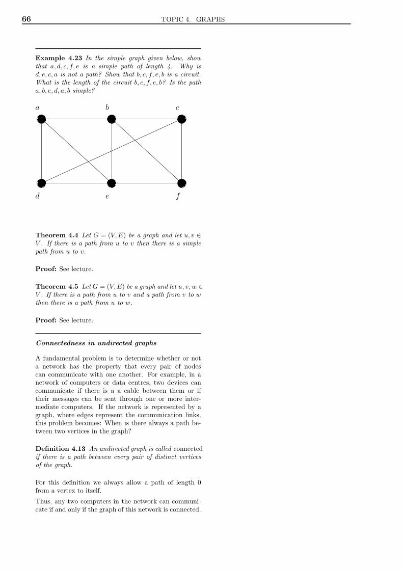
66 TOPIC 4. GRAPHS

Example 4.23 In the simple graph given below, showthat a, d, c, f, e is a simple path of length 4. Why isd, e, c, a is not a path? Show that b, c, f, e, b is a circuit.What is the length of the circuit b, c, f, e, b? Is the patha, b, e, d, a, b simple?

a b c

d e f

Theorem 4.4 Let G = (V,E) be a graph and let u, v ∈V . If there is a path from u to v then there is a simplepath from u to v.

Proof: See lecture.

Theorem 4.5 Let G = (V,E) be a graph and let u, v, w ∈V . If there is a path from u to v and a path from v to wthen there is a path from u to w.

Proof: See lecture.

Connectedness in undirected graphs

A fundamental problem is to determine whether or nota network has the property that every pair of nodescan communicate with one another. For example, in anetwork of computers or data centres, two devices cancommunicate if there is a a cable between them or iftheir messages can be sent through one or more inter-mediate computers. If the network is represented by agraph, where edges represent the communication links,this problem becomes: When is there always a path be-tween two vertices in the graph?

Definition 4.13 An undirected graph is called connectedif there is a path between every pair of distinct verticesof the graph.

For this definition we always allow a path of length 0from a vertex to itself.

Thus, any two computers in the network can communi-cate if and only if the graph of this network is connected.


Example 4.24 Is the graph G shown below connected?Why or why not? Is the graph H shown below connected?Why or why not?

a b

d

c

e

gf

h j

k

m

p

n

G H

Theorem 4.6 There is a simple path between every pairof distinct vertices of a connected undirected graph.

Proof: See lecture.

Components

A graph that is not connected is the union of two ormore connected graphs, each pair of which has no vertexin common. These disjoint connected graphs are calledthe connected components of the graph.

68 TOPIC 4. GRAPHS

Example 4.25 What are the connected components ofthe graph G shown below?

b c

fd

a

e

Paths and circuits in directed multigraphs

Definition 4.14

• A path of length n, where n is a positive integer,from u to v in a directed multigraph is a sequence ofedges e1, e2, . . . , en of the graph such that f(e1) =(x0, x1), f(e2) = (x1, x2), . . . , f(en) = (xn−1, xn),where x0 = u and xn = v. When there are nomultiple edges in the graph, this path is denoted byits vertex sequence x0, x1, x2, . . . , xn.

• A path that begins and ends at the same vertex iscalled a circuit or cycle.

• A path or circuit is called simple it does not con-tain the same edge more than once and each vertexonly appears once unless the initial vertex is thefinal vertex or there is a loop in the graph.

When it is not necessary to distinguish between mul-tiple edges, we will denote a path e1, e2, . . . , en wheref(e1) = (xi−1, xi) for i = 1, 2, . . . , n by its vertex se-quence x0, x1, . . . , xn. The notation identifies a path onlyup to the vertices it passes through. There may be morethan one path that passes through this sequence of ver-tices.

Connectedness in directed graphs

There are two notions of connectedness in directed graphs,depending on whether the directions of the edges are con-sidered. Again we declare that a vertex is always stronglyconnected with itself (by a path of length zero).

Definition 4.15 Two vertices a, b in a directed graphare strongly connected if there is a path from a to b anda path from b to a.


A directed graph is strongly connected if there is a pathfrom a to b and a path from b to a whenever a and b arevertices in the graph.

For a directed graph to be strongly connected there mustbe a sequence of directed edges from any vertex in thegraph to any other vertex. A directed graph can fail tobe strongly connected but still be in “one piece.” Tomake this precise, the following definition is given.

Definition 4.16 A directed graph is weakly connectedif there is a path between any two vertices in the under-lying undirected graph.

That is, a directed graph is weakly connected if and onlyif there is always a path between two vertices when thedirections of the edges are disregarded. Clearly, anystrongly connected directed graph is also weakly con-nected.

Theorem 4.7 Let G = (V,E) be a directed graph.

1. Every vertex is strongly connected to itself.

2. Let u, v ∈ V . If u is strongly connected to v then vis strongly connected to u.

3. Let u, v, w ∈ V . If u is strongly connected to vand v is strongly connected to w then u is stronglyconnected to w.

Proof: See lecture.

70 TOPIC 4. GRAPHS

Example 4.26 Are the directed graphs G and H shownbelow strongly connected? Are they weakly connected?

a b

c

d e

a b

c

d e

G

H

Counting paths between vertices

The number of paths between two vertices in a graph canbe determined using its adjacency matrix.

Theorem 4.8 Let G be a graph with adjacency matrix Awith respect to the ordering v1, v2, . . . , vn (with directed orundirected edges, with multiple edges and loops allowed).The number of different paths of length r from vi to vj ,where r is a positive integer, equals the (i, j)th entry ofAr.

Proof: See lecture.

4.5. EULER PATHS 71

Example 4.27 How many paths of length 4 are therefrom a to d in the simple graph G shown below?

a b

cd

G

4.5 Euler paths

We now tell a famous story in the history of graph the-ory. Back in the 18th century, the town of Konigsbergwas part of Prussia (it is now called Kaliningrad and ispart of the Russian republic). The town was dividedinto four sections by the Pregel River. These four sec-tions included the two regions on the banks of the Pregel,Kneiphof Island, and the region between the two branchesof the Pregel. In the 18th century seven bridges con-nected these regions. The image below (from the Mac-Tutor website) depicts these regions and bridges.

The people in the town enjoyed walking through the townon Sundays. They wondered whether it was possible tostart at some location in the town, travel across all thebridges without crossing any bridge twice, and return tothe starting point.

The Swiss mathematician Leonhard Euler showed thatno such Sunday stroll exists. His solution was publishedin 1736, and is considered to be the birth of graph the-ory. Euler studied this problem using the multigraph ob-tained when the four regions are represented by verticesand the bridges are represented by edges. This multi-graph is shown below.

72 TOPIC 4. GRAPHS

Euler circuits and paths

The problem of traveling across every bridge withoutcrossing any bridge more than once can be rephrasedin terms of this model. The question becomes: Is therea circuit in this multigraph that contains every edge ex-actly once? (Note that this circuit is required to visitevery edge, so it must visit vertices of degree > 2 morethan once.) This may seem an artificial problem, but ithas applications in scheduling postal delivery routes andtrash collection services.

Definition 4.17 An Euler circuit in a graph G is a sim-ple circuit containing every edge of G. An Euler path inG is a path containing every edge of G exactly once.

Example 4.28 Which of the undirected graphs belowhave an Euler circuit? Of those that do not, which havean Euler path?

a b

d

e

a b

c d

e

a b

c

de

c

G2G1

G3

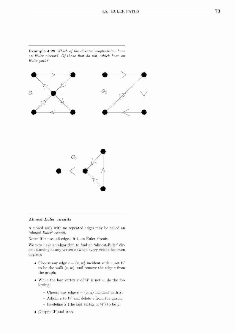
4.5. EULER PATHS 73

Example 4.29 Which of the directed graphs below havean Euler circuit? Of those that do not, which have anEuler path?

G3

G2G1

Almost Euler circuits

A closed walk with no repeated edges may be called an‘almost-Euler’ circuit.

Note: If it uses all edges, it is an Euler circuit.

We now have an algorithm to find an ‘almost-Euler’ cir-cuit starting at any vertex v (when every vertex has evendegree):

• Choose any edge e = {v, w} incident with v, set Wto be the walk (v, w), and remove the edge e fromthe graph;

• While the last vertex x of W is not v, do the fol-lowing:

– Choose any edge e = {x, y} incident with x;

– Adjoin e to W and delete e from the graph;

– Re-define x (the last vertex of W ) to be y.

• Output W and stop.

74 TOPIC 4. GRAPHS

Building larger almost-Euler circuit

Suppose T = (v0, v1, . . . , vk, v0) and U = (w0, w1, . . . , wℓ, w0)are almost-Euler circuits with a common vertex, say vi =wj , but with no edges in common.

Then we can attach T and U together at the commonvertex vi = wj to create a longer almost-Euler circuit,namely

(v0, v1, . . . , vi, wj+1, . . . , wℓ, w0, . . . , wj−1, wj , vi+1, . . . , vk, v0).

In other words, follow T from v0 to vi = wj , then followU from wj (through wℓ and w0) to wj again, and thencomplete the circuit by taking T the rest of the way fromwj = vi to v0.

Necessary and sufficient condition for Euler cir-cuits

There are simple criteria for determining whether a multi-graph has an Euler circuit or an Euler path. Euler discov-ered them when he solved the famous Konigsberg bridgeproblem. We will assume that all graphs discussed inthis section have a finite number of vertices and edges.

What can we say if a connected multigraph has an Eulercircuit? What we can show is that every vertex musthave even degree.

• To do this, first note that an Euler circuit beginswith a vertex a and continues with an edge incidentto a, say {a, b}. The edge {a, b} contributes 1 todeg(a).

• Each time the circuit passes through a vertex itcontributes 2 to the vertex’s degree, since the cir-cuit enters via an edge incident with this vertexand leaves via another such edge.

• Finally, the circuit terminates where it started, con-tributing 1 to deg(a). Therefore, deg(a) must beeven, because the circuit contributes 1 when it be-gins, 1 when it ends, and 2 every time it passesthrough a (if it ever does).

• A vertex other than a has even degree becausethe circuit contributes 2 to its degree each timeit passes through the vertex.

• We conclude that if a connected graph has an Eulercircuit, then every vertex must have even degree.

Example 4.30 Solve the Konigsberg bridge problem.

Is this necessary condition for the existence of an Eulercircuit also sufficient? That is, must an Euler circuitexist in a connected multigraph if all vertices have evendegree? The next result is one of the first big theoremsin graph theory.

4.5. EULER PATHS 75

Theorem 4.9 A connected multigraph has an Euler cir-cuit if and only if each of its vertices has even degree.

The algorithm below gives the constructive procedure forfinding Euler circuits.

procedure Euler(G: connected multigraph with all verticesof even degree)

C := a circuit in G beginning at an arbitrarily chosen ver-tex with edges successively added to form a path thatreturns to this vertex.

Initially C is empty.

H := G with the edges of C removed

while H has edges

begin

S := a circuit in H beginning at a vertex in H thatalso is an endpoint of an edge of C

H := H with edges of S and all isolated vertices re-moved

C := C with S inserted at the appropriate vertex

end {C is an Euler circuit}

Example 4.31 Many puzzles ask you to draw a picturein a continuous motion, without lifting the pencil off thepage, so that no part of the picture is retraced. We cansolve such puzzles using Euler circuits and paths. Forexample, can Mohammed’s scimitars, shown below, bedrawn in this way, where the drawing begins and ends atthe same point?

a

b

c

d

ef

i

j

k

hg

Necessary and sufficient condition for Euler paths

Theorem 4.10 A connected multigraph has an Eulerpath but not an Euler circuit if and only if it has exactlytwo vertices of odd degree.

76 TOPIC 4. GRAPHS

Example 4.32 Which graphs shown below have an Eu-ler path?

G3

G1 G2

Example 4.33 Returning to 18th-century Konigsberg,is it possible to start at some point in the town, travelacross all the bridges exactly once, and end up at someother point in town?

Example 4.34 A domino is a rectangle divided into twosquares with each square numbered one of 0, 1, . . . , 6.Two squares on a single domino can have the same num-ber. Show that the twenty-one distinct dominoes can bearranged in a circle so that touching dominoes have ad-jacent squares with identical numbers. (Hint : Considerthe complete graph K7 with vertices labeled 0, 1, . . . , 6.This has a Euler circuit since each of its vertices hasdegree 6.)

4.6 * Isomorphism of graphs

We often need to know whether it is possible to drawtwo graphs in the same way. For instance, in chemistry,graphs are used to model compounds. Different com-pounds can have the same molecular formula but can

4.6.* ISOMORPHISM OF GRAPHS 77

differ in structure. Such compounds will be representedby graphs that cannot be drawn in the same way. Thegraphs representing previously known compounds can beused to determine whether a supposedly new compoundhas been studied before.

Isomorphic graphs

Definition 4.18 The simple graphs G1 = (V1, E1) andG2 = (V2, E2) are isomorphic if there is a one-to-oneand onto function h : V1 → V2 with the property that aand b are adjacent in G1 if and only if h(a) and h(b) areadjacent in G2, for all a and b in V1. Such a function his called an isomorphism.

In other words, when two simple graphs are isomorphic,there is a one-to-one correspondence between vertices ofthe two graphs that preserves the adjacency relationship.

Example 4.35 Show that the graphs G = (V,E) andH = (W,F ), displayed below, are isomorphic.

HG

Invariant properties

It is often difficult to determine whether two simple graphsare isomorphic. There are n! possible one-to-one corre-spondences between the vertex sets of two simple graphswith n vertices. Testing each such correspondence to seewhether it preserves adjacency and nonadjacency is im-practical if n is at all large.

However, we can often show that two simple graphs arenot isomorphic by showing that they do not share a prop-erty that isomorphic simple graphs must both have. Sucha property is called an invariant with respect to isomor-phism of simple graphs. For instance:

• Isomorphic simple graphs must have the same num-ber of vertices, since there is a one-to-one corre-spondence between the sets of vertices of the graphs.

• Isomorphic simple graphs must have the same num-ber of edges, because the one-to-one correspondencebetween vertices establishes a one-to-one correspon-dence between edges.

78 TOPIC 4. GRAPHS

• The degrees of the vertices in isomorphic simplegraphs must be the same. That is, a vertex v ofdegree d in G must correspond to a vertex h(v) ofdegree d in H , since a vertex w in G is adjacent tov if and only if h(v) and h(w) are adjacent in H .

Number of vertices and edges in isomorphic graphs

The number of vertices, the number of edges, and thedegrees of the vertices are all invariants under isomor-phism. If any of these quantities differ in two simplegraphs, these graphs cannot be isomorphic.

However, when these invariants are the same, it doesnot necessarily mean that the two graphs are isomorphic.There are no useful sets of invariants currently knownthat can be used to determine whether simple graphsare isomorphic.

Example 4.36 Determine whether the graphs G and Hshown below are isomorphic.

d

gh

s

v

y

a b

c

e f

z

w x

t

u

G H

To show that a function h from the vertex set of a graphG to the vertex set of a graph H is an isomorphism, weneed to show that h preserves edges. One helpful wayto do this is to use adjacency matrices. In particular, toshow that h is an isomorphism, we can show that the ad-jacency matrix of G is the same as the adjacency matrixof H , when rows and columns are labeled to correspondto the images under h of the vertices in G that are thelabels of these rows and columns in the adjacency matrixof G.


Example 4.37 Determine whether the graphs G and Hdisplayed below are isomorphic.

a b

cd

w x

yz

G

H

Paths and isomorphism

There are several ways that paths and circuits can helpdetermine whether two graphs are isomorphic. For ex-ample, the existence of a simple circuit of a particularlength is a useful invariant that can be used to show thattwo graphs are not isomorphic. In addition, paths can beused to construct mappings that may be isomorphisms.

80 TOPIC 4. GRAPHS

Example 4.38 Determine whether the graphs shown be-low are isomorphic.

a b

c

de

f

x

r

s

z y

t

G H

We have shown how the existence of a type of path,namely, a simple circuit of a particular length, can beused to show that two graphs are not isomorphic. Wecan also use paths to find mappings that are potentialisomorphisms.

Example 4.39 Determine whether the graphs shown be-low are isomorphic.

a

b

c

d

e

v

w

x

y

z

G H


* Subgraphs

Sometimes we need only part of a graph to solve a prob-lem. For instance, we may care only about one part ofa large computer network, such as the part that involvesthe data centres in Auckland, Hamilton, Wellington, andChristchurch. We can ignore the other centres and ca-bles. In the graph model we remove the vertices cor-responding to the computer centres other than the fourof interest, and we remove all edges incident with anyvertex that was removed.

When edges and vertices are removed from a graph, with-out removing endpoints of any remaining edges, a smallergraph is obtained. Such a graph is called a subgraph ofthe original graph.

Definition 4.19 A subgraph of a graph G = (V,E) isa graph H = (W,F ) where W ⊆ V and F ⊆ E.

Notice that, in the definition of a subgraph, we must re-move any edges which have had one of their endpointsremoved. This does not mean that we may not also re-move some of the other edges. For example, for any graphG = (V,E), the graph H = (V,∅) counts as a (ratheruninteresting) example of a subgraph.

82 TOPIC 4. GRAPHS

Example 4.40 Let G be the graph shown below. Whichof the graphs H1, H2, H3 are subgraphs of G?

G

u

v

w

z

H1u

v

w

z

H2

v

w

z

u

H3

w

z

u

4.7.* HAMILTON PATHS AND CIRCUITS 83

4.7 * Hamilton paths and circuits

We have developed necessary and sufficient conditionsfor the existence of paths and circuits that contain everyedge of a multigraph exactly once. Can we do the samefor simple paths and circuits that contain every vertex ofthe graph exactly once?

Definition 4.20 A path x0, x1, . . . , xn−1, xn in the graphG = (V,E) is called a Hamilton path if

V = {x0, x1, . . . , xn−1, xn}

and xi = xj for 0 ≤ i < j ≤ n.A circuit

x0, x1, . . . , xn−1, xn, x0

(with n > 1) in a graph G = (V,E) is called a Hamiltoncircuit if x0, x1, . . . , xn−1, xn is a Hamilton path.

Hamilton’s puzzle

This terminology comes from a puzzle invented in 1857by the Irish mathematician Sir William Rowan Hamilton.Hamilton’s puzzle consisted of a wooden dodecahedron (apolyhedron with 12 regular pentagons as faces, as shownbelow, with a peg at each vertex of the dodecahedron,and string. The 20 vertices of the dodecahedron werelabeled with different cities in the world. The object ofthe puzzle was to start at a city and travel along theedges of the dodecahedron (see the following picture),visiting each of the other 19 cities exactly once, and endback at the first city. The circuit traveled was markedoff using the strings and pegs.

Example 4.41 Since we cannot supply each student witha wooden solid with pegs and string, we will consider theequivalent question: Is there a circuit in the graph shownbelow that passes through each vertex exactly once? Thissolves the puzzle since this graph is isomorphic to the

84 TOPIC 4. GRAPHS

graph consisting of the vertices and edges of the dodeca-hedron.

Example 4.42 Which of the simple graphs below have aHamilton circuit or, if not, a Hamilton path?

a

b c

d

ef

g

b c

g

ef

G1

G2

Determining whether a graph contains a Hamil-ton circuit

Is there a simple way to determine whether a graph hasa Hamilton circuit or path? At first, it might seem thatthere should be an easy way to determine this, since thereis a simple way to answer the similar question of whethera graph has an Euler circuit.

Surprisingly, there are no known simple necessary andsufficient criteria for the existence of Hamilton circuits.However, many theorems are known that give sufficientconditions for the existence of Hamilton circuits. Also,certain properties can be used to show that a graph hasno Hamilton circuit.

4.7.* HAMILTON PATHS AND CIRCUITS 85

• A graph with a vertex of degree 1 cannot have aHamilton circuit, since in a Hamilton circuit eachvertex is incident with two edges in the circuit.

• If a vertex in the graph has degree 2, then bothedges that are incident with this vertex must bepart of any Hamilton circuit.

• When a Hamilton circuit is being constructed andthis circuit has passed through a vertex, then all re-maining edges incident with this vertex, other thanthe two used in the circuit, can be removed fromconsideration.

• A Hamilton circuit cannot contain a smaller circuitwithin it.

Example 4.43 Show that neither graph displayed belowhas a Hamilton circuit.

G1 G2

Example 4.44 Show that Kn has a Hamilton circuitwhenever n ≥ 3.

The traveling salesperson problem

Suppose the drawing in Figure 4.1 is a map showing fourcities and the distances in kilometers between them. Sup-pose that a salesperson must visit each city exactly once,starting and ending in city A. Which route from city tocity will minimize the total distance that must be trav-eled?

86 TOPIC 4. GRAPHS

A

B C

D

30

50

35 25

40

30

Figure 4.1:

This problem can be solved by writing all possible Hamil-tonian circuits starting and ending at A and calculatingthe total distance traveled for each.

Route Total Distance (in kilometers)ABCDA 30+30+25+40=125ABDCA 30+35+25+50=140ACBDA 50+30+35+40=155ACDBA 140 [ABDCA backwards]ADBCA 155 [ACBDA backwards]ADCBA 125 [ABCDA backwards]

Thus either route ABCDA or ADCBA gives a minimumtotal distance of 125 kilometers.

The general traveling salesperson problem involves find-ing a Hamiltonian circuit to minimize the total distancetraveled for an arbitrary graph with n vertices in whicheach edge is marked with a distance. One way to solvethe general problem is to use the above method. Writedown all Hamiltonian circuits starting and ending at aparticular vertex, compute the total distance for each,and pick one for which this total is minimal. However,even for medium-sized values of n this method is imprac-tical. At present, there is no known algorithm for solvingthe general traveling salesperson problem that is more ef-ficient. However, there are efficient algorithms that find‘pretty good’ solutions, that is, circuits that, while notnecessarily having the least possible total distance, havesmaller total distances than most other Hamiltonian cir-cuits.

Trees

The word “tree” is used slightly differently between math-ematicians and computer scientists. For a mathemati-cian, a tree is a connected graph that contains no simplecircuits. In this sense, trees were used by Arthur Cayleyin 1857 to count certain types of chemical compounds.They have many other applications.

Trees are particularly useful in computer science. Here,it is usual to study “rooted trees”, which are trees with adistinguished vertex called the “root”. Rooted trees of-ten also have a sense of “direction”. A family tree is anexample of a rooted tree. Rooted trees allow efficient al-gorithms for locating items in a list, and the constructionof efficient codes for storing and transmitting data.

5.1 Introduction to trees

Our first example is the genealogical family tree of theBernoulli family. (This family includes a number of fa-mous Swiss mathematicians). This is a graph where thevertices represent family members and the edges repre-sent parent-child relationships. This is a rooted tree withNikolaus Bernoulli being the “root” vertex. If we forgetthe root and the “ordering” then we obtain an undirectedconnected graph with no simple circuits, which is themathematicians notion of a tree.

Nikolaus

Nikolaus I

Nikolaus II

Jacob Johann I

Nikolaus III

(1695ï1776)

Daniel Johann II

(1654ï1705)

(1623ï1708)

(1662ï1716)

(1687ï1759)

(1667ï1748)

(1710ï1782) (1710ï1790)

Johann III Jacob II(1746ï1807) (1759ï1789)

Definition 5.1 A tree is a connected undirected graphwith no simple circuits.

87

88 TOPIC 5. TREES

Since a tree cannot have a simple circuit, a tree cannotcontain multiple edges or loops. Therefore any tree mustbe a simple graph.

Example 5.1Which of the graphs shown below are trees?

(c)(a) (b) (d)

Forests

Any connected graph that contains no simple circuits isa tree. What about graphs containing no simple circuitsthat are not necessarily connected? These graphs arecalled forests and have the property that each of theirconnected components is a tree.

Example 5.2 The figure shown below displays a forest.

Unique simple paths

Trees are often defined as undirected graphs with theproperty that there is a unique simple path between everypair of vertices. The following theorem shows that thisalternative definition is equivalent to our definition.

5.1. INTRODUCTION TO TREES 89

Theorem 5.1 An undirected graph is a tree if and onlyif there is a unique simple path between any two of itsvertices.

Proof: See lecture.

Example 5.3 Prove that every tree is a bipartite graphand show that the converse of this statement is not true.

Solution. Fix any vertex v0. Let V1 be the set of all verticeswhose unique path length from v0 is even and let V2 be the set ofall vertices whose unique path length from v0 is odd.So every vertex of the tree can be partitioned into two subsets V1

and V2 such that every edge of the tree joins some vertex in V1 tosome vertex in V2.Therefore, every tree is a bipartite graph.

The converse of the statement is not true . The complete bipartitegraph K2,2 (shown below) forms a counterexample, as it has a sim-ple circuit. For more counterexamples, simply take any bipartitegraph that is not connected.

Rooted trees

In many applications of trees a particular vertex of atree is designated as the root. Once we specify a root,we can assign a direction to each edge as follows. Sincethere is a unique path from the root to each vertex of thegraph (from Theorem 5.1), we direct each edge away fromthe root. Thus, a tree together with its root produces adirected graph called a rooted tree.

We can change an unrooted tree into a rooted tree bychoosing any vertex as the root. Note that differentchoices of the root produce different rooted trees.

90 TOPIC 5. TREES

Example 5.4 The figure shown below displays the rootedtrees formed by designating a to be the root and c to bethe root, respectively, in a tree.

Root c

Root a

a

b c d a

b

c

d

e

f g

f g e

We usually draw a rooted tree with its root at the topof the graph. The arrows indicating the directions of theedges in a rooted tree can be omitted, since the choice ofroot determines the directions of the edges.

Terminology for rooted trees

The terminology for rooted trees has botanical and ge-nealogical origins. Suppose that T is a rooted tree.

• If v is a vertex in T other than the root, the parentof v is the unique vertex u such that there is adirected edge from u to v.

• When u is the parent of v, v is called a child of u.

• Vertices with the same parent are called siblings.

• The ancestors of a vertex other than the root arethe vertices in the path from the root to this vertex,excluding the vertex itself and including the root(that is, its parent, its parent’s parent, and so on,until the root is reached).

• The descendants of a vertex v are those verticesthat have v as an ancestor.

• A vertex of a tree is called a leaf (or terminal ver-tex ) if it has no children.

• Vertices that have children are called internal ver-tices. The root is an internal vertex unless it is theonly vertex in the graph, in which case it is a leaf.


• If a is a vertex in a tree, the subtree with a asits root is the subgraph of the tree consisting of aand its descendants and all edges incident to thesedescendants.

We cannot use terms like parent/child/ancestor/descendantwhen discussing un-rooted trees, but leaf (only one edge),internal vertices (at least 2 edges) make sense. The wordsubtree is a dangerous word since a subgraph of a tree isnot necessarily the same as a subtree of a rooted tree.We will try not to cause confusion with these words.

Example 5.5 In the rooted tree T (with root a) shownbelow, find the parent of c, the children of g, the siblingsof h, all ancestors of e, all descendants of b, all internalvertices, and all leaves. What is the subtree rooted at g?

a

b

c

d e

f

g

h i j

k ml

m-ary trees and binary trees

Rooted trees with the property that all of their internalvertices have the same number of children are used inmany different applications. Later in this topic we willuse such trees to study problems involving coding.

Definition 5.2 A rooted tree is called an m-ary tree ifevery vertex has no more than m children. The tree iscalled a fullm-ary tree if every internal vertex has exactlym children. An m-ary tree with m = 2 is called a binarytree.

92 TOPIC 5. TREES

Example 5.6 Are the rooted trees shown below full m-ary trees for some positive integer m?

(Full) Binary tree

3-ary tree

Full 3-ary tree

Ordered rooted tree

An ordered rooted tree is a rooted tree where the childrenof each internal vertex are ordered. Ordered rooted treesare drawn so that the children of each internal vertex areshown in order from left to right. Note that a representa-tion of a rooted tree in the conventional way determinesan ordering for its edges. We will use such orderings ofedges in drawings without explicitly mentioning that weare considering a rooted tree to be ordered.

• In an ordered binary tree, if an internal vertex hastwo children, the first child is called the left childand the second child is called the right child.


• The tree rooted at the left child of a vertex is calledthe left subtree of this vertex, and the tree rooted atthe right child of a vertex is called the right subtreeof the vertex.

The student should note that for some applications everyvertex of a binary tree, other than the root, is designatedas a right or a left child of its parent. This is done evenwhen some vertices have only one child. We will makesuch designations whenever it is necessary, but not oth-erwise.

Example 5.7 What are the left and right children ofd in the binary tree T shown below (where the order isthat implied by the drawing)? What are the left and rightsubtrees of c?

a

b c

d

e

f g

h i

j k

l

m

Given an ordered rooted tree one can consider severalmethods to list all the vertices in the tree.

One approach is called the preorder algorithm: Preorder(T )runs on a tree T with root r by printing the root, thenif x1, . . . , xk are the children (in order) the algorithmrecursively calls Preorder(T1), . . . , Preorder(Tk) whereeach Ti is the sub-tree with root xi.

The postorder algorithm is: Postorder(T ) on a tree Twith root r and children x1, . . . , xk in order runs Postorder(T1),. . . , Postorder(Tk) and then prints the root r.

Just as in the case of graphs, there is no standard ter-minology used to describe trees, rooted trees, orderedrooted trees, and binary trees. This nonstandard termi-nology occurs since trees are used extensively throughoutcomputer science, which is a relatively young field. Thestudent should carefully check meanings given to termsdealing with trees whenever they occur.

94 TOPIC 5. TREES

5.2 Some applications of trees

We now discuss some applications of trees in computerscience, chemistry, and business.

Trees in Chemistry

An important abstraction in chemistry is to write moleculesas graphs. Atoms are represented as vertices and chem-ical bonds are writted as edges. Sometimes the graphshave cycles (e.g., Benzene) but in many important casesthey are trees. Note that, in these cases, they naturallyarise as trees without a root. The English mathematicianArthur Cayley discovered trees in 1857 when he was try-ing to enumerate the isomers of compounds of the formCnH2n+2, which are called saturated hydrocarbons.

In graph models of saturated hydrocarbons, each carbonatom is represented by a vertex of degree 4, and eachhydrogen atom is represented by a vertex of degree 1.There are 3n+2 vertices in a graph representing a com-pound of the form CnH2n+2. The number of edges insuch a graph is half the sum of the degrees of the ver-tices. Hence, there are (4n+2n+2)/2 = 3n+1 edges inthis graph. Since the graph is connected and the numberof edges is one less than the number of vertices (Theorem5.2 below), it must be a tree.

The nonisomorphic trees (i.e., ones that really do corre-spond to different molecules) with n vertices of degree 4and 2n+ 2 of degree 1 represent the different isomers ofCnH2n+2. For instance, when n = 4, there are exactlytwo nonisomorphic trees of this type (it is a good exer-cise to verify this). Hence, there are exactly two differentisomers of C4H10. Their structures are displayed below.These two isomers are called butane and isobutane.

C

C

C

C

C

H

H

H

H

H

H

H

H

H

H

H

H

H

CC

C

H H

H

H

H

H

H

Butane

Isobutane

Computer file systems

Folders/directories on a computer disk have a tree struc-ture corresponding to sub-folders/sub-directories. The

5.3. PROPERTIES OF TREES 95

root directory contains the entire file system. Thus, afile system may be represented by a rooted tree, wherethe root represents the root directory, internal verticesrepresent subdirectories, and leaves represent ordinaryfiles or empty directories. One such file system is shownbelow. In this system, the file khr is in the directory rj.

rje

khr

bin

ard ple

/

5.3 Properties of trees

Counting vertices and edges in trees

We will often need results relating the numbers of edgesand vertices of various types in trees.

Theorem 5.2 A tree with n vertices has n− 1 edges.

Proof: See lecture.

The number of vertices in a full m-ary tree with a spec-ified number of internal vertices is determined, as thefollowing theorem shows. As in Theorem 5.2, we will usen to denote the number of vertices in a tree.

Theorem 5.3 A full m-ary tree with i internal verticescontains n = mi+ 1 vertices.

Proof: See lecture.

Example 5.8 Let T be a full m-ary tree with 28 vertices.What are the possible values of m?

Solution. i = 27/m. Since i must be an integer, m must be 1,3, 9, or 27.

Counting leaves

Suppose that T is a full m-ary tree with n vertices. Leti be the number of internal vertices and l the numberof leaves in this tree. Once one of n, i, and l is known,the other two quantities are determined. How to find theother two quantities from the one that is known is givenin the following theorem.

96 TOPIC 5. TREES

Theorem 5.4 A full m-ary tree

1. with n vertices has

• i = (n− 1)/m internal vertices and

• l = [(m− 1)n+ 1]/m leaves,

2. with i internal vertices has

• n = mi+ 1 vertices and

• l = (m− 1)i+ 1 leaves,

3. with l leaves has

• n = (ml − 1)/(m− 1) vertices and

• i = (l − 1)/(m− 1) internal vertices.

Proof: See lecture.

Example 5.9 Suppose that someone starts a chain letter.Each person who receives the letter is asked to send it onto four other people. Some people do this, but others donot send any letters. How many people have seen theletter, including the first person, if no one receives morethan one letter and if the chain letter ends after therehave been 100 people who read it but did not send it out?How many people sent out the letter?

Height and levels

For many applications it is desirable to use rooted treesthat are “balanced,” so that the subtrees at each vertexcontain paths of approximately the same length. Somedefinitions will make this concept clear.

• The level of a vertex v in a rooted tree is the lengthof the unique path from the root to this vertex. Thelevel of the root is defined to be zero.

• The height of a rooted tree is the maximum of thelevels of vertices. In other words, the height of arooted tree is the length of the longest path fromthe root to any vertex.

5.3. PROPERTIES OF TREES 97

Example 5.10 Find the level of each vertex in the rootedtree shown below. What is the height of this tree?

a

b c d

e f g h

j

p

nmlki

Example 5.11 Let T be a full m-ary tree with 50 ver-tices. What must m be if T has height 2?

Solution. i = 49/m. Since i must be an integer, m must be 1,7, or 49.

If m = 1, then a tree of height 2 has precisely 3 vertices.

If m = 7, then a tree of height 2 with 50 vertices can exist.

If m = 49, then T has precisely 1 internal vertex and hence height1.

So if T has height 2, then it m = 7.

Balance

A rooted m-ary tree of height h is called balanced if allleaves are at levels h or h− 1.

Is the rooted tree shown above balanced? Draw a treethat is not balanced.

The following results relate the height and the numberof leaves in m-ary trees.

Theorem 5.5 There are at most mh leaves in an m-arytree of height h.

Proof: See lecture.

98 TOPIC 5. TREES

Corollary 5.1 If an m-ary tree of height h has l leaves,then h ≥ ⌈logm l⌉. If the m-ary tree is full and balanced,then h = ⌈logm l⌉. (We are using the ceiling functionhere. Recall that ⌈x⌉ is the smallest integer greater thanor equal to x.)

5.4 Expression trees

Arithmetic expressions

Mathematical expressions that consist of integers and in-teger variables, combined together using addition, sub-traction and multiplication, are called arithmetic expres-sions.

Some examples are 0, 2, x, y, 2+x, x ·y, ((x ·y)−(2+x))and ((x · y)− (2 + x)) + y.

Arithmetic expressions can be defined inductively as fol-lows:

• Integer variables and integers are arithmetic ex-pressions.

• If A and B are arithmetic expressions, then so areA+B, A−B and A ∗B (= A ·B).

Expression trees

Every arithmetic expression can be represented by a tree,called an expression tree. For example, (x − y) ∗ ((x +9)− 4) can be represented by

∗

− −

x y + 4

x 9

Inductive definition of an expression tree

Let Te be the tree representing the arithmetic expressione.

Basis: If e is an integer or integer variable, take Te as asingle vertex labelled e.

Induction: If e is of the form A ⋄B (where ⋄ is +, − or·), then take the expression trees TA and TB (for A andB), and create Te by introducing a new root vertex withlabel ⋄, and new edges from this vertex to the roots ofTA and TB.

•

• •

⋄

TA TB

5.5. SPANNING TREES 99

Theorem 5.6 In an expression tree T , every leaf is la-belled with an integer or integer variable, and every in-terior vertex is labelled with +, · or −.

Proof: We use induction on the number of vertices.

Basic step: If T has one vertex then the expression isa single integer or integer variable, and that vertex is aleaf (and there are no interior vertices), so the conclusionholds.

Inductive step: Suppose T has more than one vertex.Then T is the tree for an expression of the form A ⋄ B,with root labelled ⋄. By induction, we may suppose TA

and TB have the required properties. Now every leaf ofT is a leaf of TA or TB, and so is labelled with an integeror integer variable, while every interior vertex of T otherthan the root is an interior vertex of TA or TB, so islabelled with +, · or −.

5.5 Spanning trees

Consider the system of roads in the North Island repre-sented by the simple connected graph shown below. Ifit snows, the only way a road can be kept open is us-ing a snow-plough, but this costs a lot of money. Thetransport department wants to plough the fewest roadsso that it will be possible to drive between any pair oftowns. How can this be done?

Tirau

Tauranga

Waioru

National Park

Ohakune

Taupo

At least five roads must be ploughed to ensure that thereis a path between any two towns. Note that the subgraphrepresenting these roads is a tree, since it is connectedand contains six vertices and five edges.

This problem was solved with a connected subgraph withthe minimum number of edges containing all vertices ofthe original simple graph. Such a graph must be a tree.

Definition 5.3 Let G be a simple graph. A spanningtree of G is a subgraph of G that is a tree containingevery vertex of G.

A simple graph with a spanning tree must be connected,since there is a path in the spanning tree between any

100 TOPIC 5. TREES

two vertices. The converse is also true; that is, everyconnected simple graph has at least one spanning tree.We will give an example before proving this result.

Example 5.12 Find a spanning tree of the simple graphG shown below.

u w

xyz

Another characterization of connected graphs

Theorem 5.7 A simple graph is connected if and onlyif it has a spanning tree.

Proof: See lecture.

Sets, Relations and Functions

6.1 Sets

A set is a collection of objects. The objects in the setare called the elements of the set. We indicate that theobject x is an element of the set A by writing x ∈ A:otherwise, we write x /∈ A.

We have three basic ways of specifying a particular set;enumeration, comprehension and replacement.

Enumeration to describe a set by enumeration, we listthe elements. The order is unimportant, and itmakes no difference if we list an element more thanonce. So the following specifications are equivalent:

A = {2, 4, 6, 8}A = {6, 8, 4, 2}A = {2, 4, 2, 6, 2, 8}

Comprehension or Abstraction to describe a set bycomprehension, we give some rule to determine whetheror not a given object is in the set. To use the sameexample as above, we have

A = { x : x is an even integer and 2 ! x ! 8 }

This is also often called “set builder” notation. Someauthors use the symbol | instead of :, e.g., A = {2n |n ∈ Z, 1 ! n ! 4}.

Replacement to describe a set by replacement, we takesome set we already know and specify some rulefor obtaining the elements of the new set from theelements of the old one. For example, if B ={1, 2, 3, 4} then

A = { 2x : x ∈ B }

When we use enumeration, we may need to use threedots, . . . , for example to describe {1, 2, . . . , 20} or {0, 1, 2, . . .}.When we use comprehension, we abbreviate

{ x : x ∈ S and P (x) } by { x ∈ S : P (x) }.

Notation

We also have standard symbols for the following sets:

∅ The empty set, which has no elements.

N The set of natural numbers, {0, 1, 2, . . .}.(This notation is not standard; some authors de-note this as Z≥0.)

101

102 TOPIC 6. SETS, RELATIONS AND FUNCTIONS

P The set of positive integers, {1, 2, 3, . . .}.

(This notation is not standard; some authors de-note this as N or Z≥1.)

Z The set of integers.

Q The set of rational numbers,

{ m

n: m ∈ Z, n ∈ P }.

R The set of real numbers.

Subsets, equality of sets, power set

Let A and B be sets. We say that A is a subset of B,written A ⊆ B, if every element of A is an element of B.For example, every natural number is a real number, soN ⊆ R. Notice that ∅ ⊆ A for every set A.

Again, let A and B be sets. We say that A and B areequal , written A = B, if they have exactly the sameelements. Note that there is no notion of “repeated”elements in a set, so that {1, 1, 1, 2, 2, 3}= {1, 2, 3}.

Example 6.1

{ x ∈ R : x2 − 5x+ 6 = 0 } = .

Notice that if A = B then A ⊆ B and B ⊆ A, andconversely if A ⊆ B and B ⊆ A then A = B.

Example 6.2 Let A = {1}, B = {1, {1}} and C ={2, 3, {1, 2, 3}}.

The integer 1 is an element of A, so 1 ∈ A. Similarly,1 ∈ B and 1 ∈ C. The set B also contains the element{1}. So we can say {1} ∈ B and {1} ∈ A. Similarly,2 ∈ C and {1, 2, 3} ∈ C.

We have A ⊆ A, A ⊆ B and A ⊆ C.

We also have A ∈ A since A does not contain the element{1}, but, as we said, A ∈ B since B does contain theelement A = {1}.

6.2. SET OPERATIONS 103

Example 6.3 Let A = { x ∈ Z : x = 2p, p ∈ Z },B = { y ∈ Z : y = 2q + 2, q ∈ Z },andC = { z ∈ Z : z = 3r − 1, r ∈ Z }.

(a) Is A = B?

(b) Is A = C?

Solution.

(a) Yes. We need to show that A ⊆ B and B ⊆ A.Take a ∈ A. Then a = 2p for some p ∈ Z. If we setq = p − 1, then q ∈ Z and a = 2p = 2(q + 1) = 2q + 2 soa ∈ B.Therefore, A ⊆ B.Next, take b ∈ B. Then b = 2q+2 for some q ∈ Z. If we setp = q+1, then p ∈ Z and b = 2(p − 1)+2 = 2p − 2+2 = 2p.So b ∈ A. Therefore, B ⊆ A.Since A ⊆ B and B ⊆ A, we have A = B.

(b) No. 4 ∈ A since 4 = 2(2). But 4 /∈ C since if it were, then4 = 3r − 1, so r = 5

3 /∈ Z. So 4 /∈ C, and A = C

Power Set

Given a set A we can form the power set of A, denotedby P(A), containing all the subsets of A.

Example 6.4 If A = {1, 2} then

P(A) =

We will show later that if A has n elements then P(A)has 2n elements.

6.2 Set operations

We can form new sets from old ones using the operationsof union, intersection and complement. Given two setsA and B, we define

• the union of A and B, written A ∪B, by

A ∪B = { x : x ∈ A or x ∈ B }.

[NB. we use “inclusive or”, in other words the abovemeans “x ∈ A, or x ∈ B, or possibly both”]

• the intersection of A and B, written A ∩B, by

A ∩B = { x : x ∈ A and x ∈ B }.

• the relative complement or difference of B with re-spect to A, written A \B, by

A \B = { x : x ∈ A and x /∈ B }.


The easiest way to visualize these is by using Venn dia-grams: we draw circles to represent the sets A andB, andshade the regions we are interested in. Note that Venndiagrams have limited use when considering more com-plex problems, and they are not acceptable as a methodof proof.

Universal set

It is sometimes useful to fix some universal set U , and saythat we are only interested in elements of U and subsetsof U . For example, we might take U = N or U = R. Ifwe have fixed some universal set U , and A ⊆ U , then wedefine the absolute complement of A, written A, by

A = {x ∈ U : x /∈ A }.

In other words, A = U \ A. In a Venn diagram, werepresent U by a rectangular box containing all the othersets.

Notice that A \B = A ∩B.

Laws for combining sets

The operations we have described satisfy certain laws,similar to the commutative law x + y = y + x and thedistributive law x(y+z) = xy+xz for real numbers. Forany subsets A, B and C of a universal set U we have

A = A Double complement

A ∩B = B ∩A CommutativeA ∪B = B ∪A

A ∩ (B ∩ C) = (A ∩B) ∩ C AssociativeA ∪ (B ∪ C) = (A ∪B) ∪ C

A ∩ (B ∪ C) = (A ∩B) ∪ (A ∩C) DistributiveA ∪ (B ∩ C) = (A ∪B) ∩ (A ∪C)

A ∩ A = A IdempotentA ∪ A = A

A \ (B ∩ C) = (A \B) ∪ (A \ C)A \ (B ∪ C) = (A \B) ∩ (A \ C)

(B ∩ C) = B ∪C De Morgan’s(B ∪ C) = B ∩C

Proof of laws

We won’t prove all of these here: we will just give oneexample of how to prove them.

If A, B and C are sets, then

A ∩ (B ∪C) = (A ∩B) ∪ (A ∩ C).

Proof: We will first show the lhs is a subset of the rhs.Suppose x ∈ A ∩ (B ∪ C). Then x ∈ A and x ∈ B ∪ C.

6.2. SET OPERATIONS 105

Since x ∈ B ∪ C, x ∈ B or x ∈ C. Hence (x ∈ A) ∧ (x ∈B∨x ∈ C). Now we apply the distributive law for ∧ and∨, to deduce that (x ∈ A ∧ x ∈ B) ∨ (x ∈ A ∧ x ∈ C).This implies that x ∈ A ∩ B or x ∈ A ∩ C, and so x ∈(A ∩B) ∪ (A ∩ C). Hence

A ∩ (B ∪ C) ⊆ (A ∩B) ∪ (A ∩ C). (∗)

We now show that (A∩B)∪ (A∩C) ⊆ A∩ (B ∪C). Lety ∈ (A ∩ B) ∪ (A ∩ C). Then y ∈ A ∩ B or y ∈ A ∩ C.So (y ∈ A ∧ y ∈ B) ∨ (y ∈ A ∧ y ∈ C). Applying thedistributive rule again we find (y ∈ A) ∧ (y ∈ B ∨ y ∈C). This means y ∈ A and y ∈ B ∪ C. So we havey ∈ A ∩ (B ∪C). Hence

(A ∩B) ∪ (A ∩ C) ⊆ A ∩ (B ∪ C).

Combining this with (∗), we get

A ∩ (B ∪ C) = (A ∩B) ∪ (A ∩ C),

as required.

Example 6.5 Prove that A ∩B = A∪B by showing thateach set is a subset of the other.

Proof: Suppose that x ∈ A ∩B

It follows that x ∈and so ¬ .

Thus x ∈ A x ∈ B.

Hence

This shows that ⊆ .

Now suppose that x ∈ A ∪B.

Then ∨It follows that ¬Hence, x A ∩B

Therefore x ∈This demonstrates that ⊆ .

Since we have demonstrated that each set is a subset ofthe other, these two sets must be equal and the identityis proved.

Cardinality

If A is a finite set, we denote the number of elements ofA, (cardinality of A), by |A|.


Example 6.6 Let A = {2, 3, 5, 7, 11, 13} andB = {1, 3, 5, 7, 9}

Find |A|, |B|, |A \B|, |B \A|, |A ∪B|, |A ∩B|.

Solution. |A| = 6|B| = 5|A \B| = |{2, 11, 13}| = 3|B \A| = |{1, 9}| = 2|A ∪ B| = |{1, 2, 3, 5, 7, 9, 11, 13}| = 8|A ∩ B| = |{3, 5, 7}| = 3

6.3 Ordered pairs, Cartesian products

Given two objects x and y, we can form the ordered pair(x, y). Unlike the pair set {x, y}, the order in which theelements appear is important: given two ordered pairs(x, y) and (u, v), we have

(x, y) = (u, v) ⇔ x = u and y = v.

Similarly, we have ordered triples (x, y, z), ordered 4-tuples (w, x, y, z), and so on, where if (x1, x2, . . . , xn) and(y1, y2, . . . , yn) are ordered n-tuples then

(x1, x2, . . . , xn) = (y1, y2, . . . , yn)⇔ xi = yi

for i = 1, 2, . . . , n.

Cartesian product

Given sets A and B, we form the Cartesian product of Aand B, written A×B, defined by

A×B = { (a, b) : a ∈ A, b ∈ B }.

If A and B are finite sets then |A×B| = |A| · |B|.

If A1, A2, . . . , An are sets, we define A1×A2× · · ·×An

to be the set of all n-tuples (a1, a2, . . . , an) where ai ∈ Ai

for i = 1, 2, . . . , n.

We sometimes write An for A× A× · · ·×A︸︷︷︸n times

. In partic-

ular, we often write A2 for A×A.

Example 6.7 The grid of squares used in the game ofbattleships is the example

{1, 2, 3, 4, 5, 6, 7, 8}× {a, b, c, d, e, f, g, h}

of a Cartesian product.

6.4. RELATIONS 107

a

b

c

d

e

fg

h

1 2 3 4 6 7 85

a

b

c

d

e

fg

h

1 2 3 4 6 7 85

Example 6.8 What is the Cartesian product A×B×Cwhere A = {0, 1}, B = {1, 2}, and C = {0, 1, 2}? Whatis (A×B)× C?

6.4 Relations

Let A and B be sets. A binary relation from A to B isa subset of A×B. A binary relation on A is a subset ofA×A.

We use binary relations to represent relationships be-tween the elements of A and the elements of B. If R isa binary relation from A to B, and (x, y) ∈ A×B, then(x, y) ∈ R if and only if the relationship holds betweenthe element x and the element y.

Example 6.9 Take A = {1, 2, 3}, and let R be the rela-tion on A defined by

(x, y) ∈ R ⇔ x < y.

Then we have R = {(1, 2), (1, 3), (2, 3)}.

Example 6.10 Let A be the set of students at Auck-land University, and let B be the set of courses. Let Rbe the relation that consists of those pairs (a, b) where ais a student in course b. For instance, if Sooyoun Leeand Wiremu Ngata are enrolled in 225, the pair (Sooy-oun Lee, 225) and (Wiremu Ngata, 225) belong to R. IfSooyoun Lee is also enrolled in 220, then the pair (Sooy-oun Lee, 220) is also in R. However, if Wiremu Ngata isnot enrolled in 220, then the pair (Wiremu Ngata, 220)is not in R.


Properties of relations

We often use infix notation for relations. In other words,we write (x, y) ∈ R as x R y. This is particularly com-mon with relations like <, =, ⊆ and so on that havestandard names. If (x, y) /∈ R, we write x R y.

There are various properties that a relation on a setmight or might not have. We say that a relation R on aset A is

• reflexive if for all x ∈ A, x R x.

• symmetric if for all x, y ∈ A, if x R y then y R x.

• antisymmetric if for all x, y ∈ A, if x R y and y R xthen x = y.

• transitive if for all x, y, z ∈ A, if x R y and y R zthen x R z.

Example 6.11 Consider the relation = on any set A.Which of the above properties hold?

Example 6.12 Consider the relation < on R. Which ofthe above properties hold?

Example 6.13 Consider the relation | on Z, defined by

a | b ⇔ for some c ∈ Z, b = ac.

Which of the above properties hold?

Example 6.14 Can a relation be both symmetric andantisymmetric?

Example 6.15 A relation on a finite set S can be pic-tured as a directed (pseudo)graph. Let the vertex set ofthe graph be S and the pairs (x, y) satisfying the relationare represented as directed edges (x, y). Draw the relation| on the set S = {1, 2, 3, 4, 5, 6}.

6.5. EQUIVALENCE RELATIONS 109

6.5 Equivalence relations

Let A be a set. An equivalence relation on A is a binaryrelation on A that is reflexive, symmetric and transitive.We often use symbols like ∼ , ≡ and ∼= for equivalencerelations.

Example 6.16 On the set of students attending Auck-land University, define one student to be related to an-other whenever their surnames begin with the same letter.Is this an equivalence relation?

Example 6.17 Let S denote the set of all people in NewZealand. Define a relation R on S by letting x R y meanthat x has the same mother as y. Is this an equivalencerelation?

Does the answer change if we define x R y to mean thatx has the same mother or father as y?

Example 6.18 Consider the set Z of integers. Fix someinteger m > 1. Then the relation of congruence modulom, defined by

x≡y (mod m) ⇔ m | x− y,

is an equivalence relation.

Example 6.19 Let G = (V,E) be a simple graph. Con-sider the binary relation on V such that, for u, v ∈ V ,u R v if and only if there is a path from u to v. This isan equivalence relation, which we call connectivity.

Example 6.20 Let C denote the set of all computerprograms. Define a relation ∼ on C as follows: ForC,C′ ∈ C (in other words, for any two computer pro-grams C and C′) we write C ∼ C′ if, for all possibleprogram inputs x, either C and C′ both do not terminateon input x, or else both C and C′ terminate on input xand return the same output.


Example 6.21 Let f : A → B be a function. Then therelation ∼ f on A, defined by

x ∼ f y ⇔ f(x) = f(y)

is an equivalence relation. We call this relation the equiv-alence relation induced by f .

Equivalence classes, partitions

Let ∼ be an equivalence relation on a set A, and letx ∈ A. The equivalence class of x under ∼ , denoted by[x], is the set of all elements of A that are related to xunder ∼ , i.e.

[x] = { y ∈ A : x ∼ y }

We denote the set of equivalence classes of elements of Aunder ∼ by [A] or by A/∼ .

Example 6.22 Consider the relation of congruence mod-ulo 2 on the set Z. What are [0], [1]?

Example 6.23 Let G be a simple graph and let R be therelation of connectivity. The equivalence classes are theconnected components of the graph.

Solution. [1] = {1, − 1}, [14] = {14, − 14}, and [0] = {0}.

Equivalence class lemma

If ∼ is an equivalence relation on A, and x, y ∈ A, thenthe following are equivalent:

1. x ∼ y.

2. [x] = [y].

3. [x] ∩ [y] = ∅.

Proof: We show that (1) implies (2), (2) implies (3)and (3) implies (1).

(1)⇒ (2) Suppose x ∼ y. Let z ∈ [y]. Then y ∼ z, sowe have x ∼ y ∼ z, and so by transitivity we havex ∼ z. Thus z ∈ [x]. Hence [y] ⊆ [x]. Conversely,let w ∈ [x]. Then x ∼ w, so by symmetry we havew ∼ x. So w ∼ x ∼ y, and so w ∼ y. Hence y ∼ w,so w ∈ [y]. Thus [x] ⊆ [y], so [x] = [y].

(2)⇒ (3) Suppose [x] = [y]. Then [x] ∩ [y] = [x] ∩ [x] =[x]. By reflexivity, x ∼ x, so x ∈ [x], so [x] = ∅.Thus [x] ∩ [y] = ∅.

6.6. PARTIAL ORDERINGS 111

(3)⇒ (1) Suppose [x] ∩ [y] = ∅. Let z ∈ [x] ∩ [y]. Thenx ∼ z and y ∼ z. By symmetry, we have z ∼ y, sox ∼ z ∼ y, and therefore by transitivity we havex ∼ y.

Hence (1), (2) and (3) are equivalent.

In other words, if [x] and [y] are equivalence classes theneither [x] = [y] or [x] and [y] are disjoint. We say thatthe relation ∼ partitions the set A.

Definition 6.1 A (finite) partition of a set X is a set{X1, . . . , Xt} where Xi ⊆ X, Xi = ∅ and:

1. Xi ∩Xj = ∅ when 1 ! i < j ! t;

2. X1 ∪X2 ∪ · · · ∪Xt = X.

An example of a partition is cutting a cake into pieces:No slice of cake is empty, slices of cake have no crumbsin common, putting the slices together forms the wholecake.

Example 6.24 Let R be the relation on Z such thatx R y if and only if x = y or x = −y. Show that R is anequivalence relation. What are [1], [−14], and [0]?

Solution. [1] = {1, − 1}, [14] = {14, − 14}, and [0] = {0}.

The graph representing an equivalence relation on a finiteset is a union of complete graphs (with loops at everyvertex).

6.6 Partial orderings

Introduction

A commonly used type of relation is an ordering. Forinstance, words in a dictionary are ordered using a re-lation called “lexicographical ordering”. We also orderreal numbers and integers in familiar ways.

Consider the usual ordering on Z. Then the set of inte-gers satisfying the relation is {(x, y) ∈ Z2 | x ! y}. Onecan verify that this relation is reflexive, antisymmetric,and transitive. Other relations that have these propertiescan be considered to be somehow “analogous” to familiarorderings.

Poset

A relation R on a set S is called a partial ordering orpartial order if it is reflexive, antisymmetric, and transi-tive. A set S together with a partial ordering R is calleda partially ordered set, or poset, and is denoted by (S,R).


Example 6.25 Show that the “greater than or equal”relation (≥) is a partial ordering on the set of integers.

Example 6.26 The divisibility relation | is a partial or-dering on the set of positive integers P = Z≥1, since itis reflexive, antisymmetric, and transitive, as was shownin Example 6.4. We see that (P, |) is a poset.

Example 6.27 Show that the inclusion relation ⊆ is apartial ordering on the power set of a set S.

Example 6.28 Let A be the set of all strings over thealphabet {0, 1}. We say that x ∈ A is a prefix of y ∈ Aif y = xv for some v ∈ A. For example 01 is a prefix of01111, while 01 is not a prefix of 1111. Show that thisrelation is a partial ordering.

Example 6.29 Let S be the set of all students in COMP-SCI 225. Define a partial ordering ≼ such that x ≼ y ifand only if x’s height is less than or equal to y’s height.Is (S, ≼ ) a poset?

Notation

In a poset the notation a ≼ b denotes that (a, b) ∈ R.This symbol is used to emphasise the similarity to thefamiliar “less than or equal to” relation. But be careful:Just because a relation is denoted by a symbol like ≼does not automatically imply it has exactly the sameproperties as !. We write a ≺ b to mean a ≼ b, buta = b. Also, we say “a is less than b” or “b is greaterthan a” if a ≺ b.

Comparable

When a and b are elements of the poset (S, ≼ ), it is notnecessary that either a ≼ b or b ≼ a. For instance, in(P(Z),⊆), {1, 2} is not related to {1, 3}, and vice versa,since neither set is contained within the other. Similarly,in (P, |), 2 is not related to 3 and 3 is not related to 2,since 2 "3 and 3 "2. This leads to the following definition.


The elements a and b of a poset (S, ≺ ) arecalled comparable if either a ≼ b or b ≼ a.When a and b are elements of S such thatneither a ≼ b nor b ≼ a, a and b are calledincomparable.

Example 6.30 In the poset (P, |), are the integers 3 and9 comparable? Are 5 and 7 comparable?

Example 6.31 In the poset (P(S),⊆), where S = {a, b, c},{a} is not comparable to {b}, and {a, b} is not comparableto {b, c}.

Totally ordered set

The adjective “partial” is used to describe partial order-ings since pairs of elements may be incomparable. Whenevery two elements in the set are comparable, the relationis called a total ordering.

Definition 6.2 If (S, ≼ ) is a poset and every two ele-ments of S are comparable, S is called a totally orderedor linearly ordered set, and ≼ is called a total order or alinear order. A totally ordered set is also called a chain.

Example 6.32 The poset (Z,!) is totally ordered, sincea ! b or b ! a whenever a and b are integers.

Example 6.33 The poset (P, |) is not totally orderedsince it contains elements that are incomparable, suchas 5 and 7.

Well ordered set

We say that (S, ≼ ) is a well-ordered set if it is a poset suchthat ≼ is a total ordering and such that every nonemptysubset of S has a least element. (a is a least element of(S, ≼ ) if a ≼ b for all b ∈ S.)


Example 6.34 The most familiar example of a well-ordered set is the set (N,!) of natural numbers, with theusual “less than or equals” ordering.

Example 6.35 The set of ordered pairs of positive in-tegers, P × P, with (a1, a2) ≼ (b1, b2) if a1 < b1, or ifa1 = b1, and a2 ! b2 (the lexicographic ordering), is awell-ordered set.

Example 6.36 The set Z, with the usual ! ordering, isnot well ordered since the set of negative integers, whichis a subset of Z, has no least element.

Lexicographic order

The letters of the alphabet have a standard ordering ‘a’< ‘b’ < · · · < ‘z’. The “dictionary” or “lexicographic”ordering turns this ordering on letters into an orderingon words. This is a special case of a general principle:given an alphabet set A that is a poset one can impose anordering on strings over the alphabet A. We now explainthis construction.

First, we will show how to construct a partial orderingon the Cartesian product of two posets, (A1, ≼ 1) and(A2, ≼ 2). The lexicographic ordering ≼ on A1 × A2 isdefined by specifying that one pair is less than a secondpair if the first entry of the first pair is less than (in A1)the first entry of the second pair, or if the first entries areequal, but the second entry of this pair is less than (inA2) the second entry of the second pair. In other words,(a1, a2) is less than (b1, b2), that is

(a1, a2) ≺ (b1, b2),

either if a1 ≺ 1 b1 or if both a1 = b1 and a2 ≺ 2 b2.

We obtain a partial ordering ≼ by adding equality to theordering ≺ on A × B. The verification of this is left asan exercise.

Example 6.37 Determine whether (3, 5) ≺ (4, 8), whether(3, 8) ≺ (4, 5), and whether (4, 9) ≺ (4, 11) in the poset(Z × Z, ≼ ), where ≼ is the lexicographic ordering con-structed from the usual ! relation on Z.

Example 6.38 On Figure 6.1, indicate the set of or-


dered pairs in P× P that are less than (3, 4).

. . .

. . .

. . .

. . .

. . .

. . .

. . .

......

......

......

......

...

(1,7) (2,7) (3,7) (4,7) (5,7) (6,7) (7,7) (8,7) (9,7)

(1,4)

(1,6)

(1,5)

(1,3)

(1,2)

(1,1) (2,1)

(9,6)

(9,5)

(9,4)

(9,3)

(9,2)

(9,1)(8,1)(7,1)(6,1)(5,1)(4,1)(3,1)

(2,2)

(3,3)

(5,5)

(6,6) (8,6)

(8,5)

(8,4)

(8,3)

(8,2)

(7,6)

(7,5)

(7,4)

(7,3)

(7,2)

(6,5)

(6,4)

(6,3)

(6,2)

(5,6)(4,6)(3,6)(2,6)

(2,5)

(2,4)

(2,3)

(3,5)

(3,4)

(3,2)

(4,5)

(4,3)

(4,4)

(4,2)

(5,4)

(5,3)

(5,2)

Figure 6.1:

Cartesian product of posets

A lexicographic ordering can be defined on the Cartesianproduct of n posets (A1, ≼ 1), (A2, ≼ 2), . . . , (An, ≼ n). De-fine the partial ordering ≼ on A1 ×A2 × · · ·×An by

(a1, a2, . . . , an) ≺ (b1, b2, . . . , bn)

if a1 ≺ 1 b1, or if there is an integer i > 0 such thata1 = b1, . . . , ai = bi, and ai+1 ≺ i+1 bi+1. In other words,one n-tuple is less than a second n-tuple if the entry ofthe first n-tuple in the first position where the two n-tuples disagree is less than the entry in that position inthe second n-tuple.

Example 6.39 Note that (1, 2, 3, 5) ≺ (1, 2, 4, 3), sincethe entries in the first two positions of these 4-tuplesagree, but in the third position the entry in the first 4-tuple, 3, is less than that in the second 4-tuple, 4. (Herethe ordering on 4-tuples is the lexicographic ordering thatcomes from the usual “less than or equals” relation on theset of integers.)

Lexicographic ordering of strings

Consider the strings ala2 · · · am and b1b2 · · · bn on a par-tially ordered set S. Suppose these strings are not equal


in length. Let t be the minimum of m and n. The defini-tion of lexicographic ordering is that the string a1a2 · · · amis less than b1b2 · · · bn if and only if

(a1, a2, . . . , at) ≺ (b1, b2, . . . , bt), or(a1, a2, . . . , at) = (b1, b2, . . . bt) and m < n,

where ≺ in this inequality represents the lexicographicordering of St. In other words, to determine the orderingof two different strings, the longer string is truncated tothe length of the shorter string, namely, to t = min(m,n)terms. Then the t-tuples made up of the first t terms ofeach string are compared using the lexicographic orderingon St. One string is less than another string if the t-tuplecorresponding to the first string is less than the t -tupleof the second string, or if these two t-tuples are the same,but the second string is longer. The verification that thisis a partial ordering is left as an exercise.

Directed graph

We can draw a directed graph of a poset (called a Hassediagram or lattice diagram) as follows. Each element ofthe poset is represented by a dot, called a vertex. Anarrow, called a directed edge, is drawn from element a toelement b if a ≼ b. The diagram in Figure 6.2(a) is adigraph of the poset ({1, 2, 3, 4},!).

Redundant edges

Many edges in the directed graph for a finite poset donot have to be shown since they must be present. Forinstance, consider the directed graph for the partial or-dering {(a, b) | a ! b} on the set {l, 2, 3, 4}, shownin Figure 6.2(a). Since this relation is a partial order-ing, it is reflexive, and its directed graph has loops at allvertices.

Consequently, we do not have to show these loops sincethey must be present; in Figure 6.2(b) loops and arrowsare not shown.


4

3

2

1

(a)

4

3

2

1

(b)

4

3

2

1

(c)

Figure 6.2:

Because a partial ordering is transitive, we do not haveto show those edges that must be present because oftransitivity. For example, in Figure 6.2(c) the edges(1, 3), (1, 4), and (2, 4) are not shown since they mustbe present. If we assume that all edges are pointed “up-ward” (as they are drawn in the figure), we do not haveto show the directions of the edges; Figure 6.2(c) doesnot show directions.

Hasse diagrams

To draw the diagram, execute the following procedure.Start with the directed graph for this relation. Draw itso that arrows are always pointing upwards. Because apartial ordering is reflexive, a loop is present at everyvertex. Remove these loops. Remove all edges whosepresence is imposed by transitivity. For instance, if (a, b)and (b, c) are in the partial ordering, remove the edge(a, c), since it must be present also. Furthermore, if (c, d)is also in the partial ordering, remove the edge (a, d),since is must be present also. Finally, arrange each edgeso that its initial vertex is below its terminal vertex (asit is drawn on paper). Remove all the arrows on thedirected edges, since the direction on the edges is nowindicated by which vertices are “higher” on the page.Note that Hasse diagrams never have horizontaledges!

These steps are well-defined, and only a finite number ofsteps need to be carried out for a finite poset. When allthe steps have been taken, the resulting diagram containssufficient information to find the partial ordering. Thisdiagram is called a Hasse diagram, named after the 20thcentury German mathematician Helmut Hasse.


Example 6.40 Draw the Hasse diagram representing thepartial ordering {(a, b) : a | b} on {1, 2, 3, 4, 6, 8, 12}.

Example 6.41 Draw the Hasse diagram for the poset(P(S),⊆), where S is the set {a, b, c}.

Maximal and minimal elements

For many applications it is useful to be able to identifycertain extremal elements of partially ordered students.For example, a prize might be given to the student in acourse with the highest grade.

An element of a poset is called maximal if it is not lessthan any element of the poset. That is, a is maximal inthe poset (S, ≼ ) if there is no b ∈ S such that a ≺ b.Similarly, an element of a poset is called minimal if it isnot greater than any element of the poset. That is, a isminimal if there is no element b ∈ S such that b ≺ a.Maximal and minimal elements are easy to spot usinga Hasse diagram. They are the elements with nothingabove them or with nothing below them.

Example 6.42 Which elements of the poset

({2, 4, 5, 10, 12, 20, 25}, |)

are maximal, and which are minimal?

Greatest and least elements

Sometimes there is an element in a poset that is greaterthan every other element. Such an element is called thegreatest element. That is, a is the greatest element of theposet (S, ≼ ) if b ≼ a for all b ∈ S. The greatest elementis unique when it exists. Likewise, an element is calledthe least element if it is less than all the other elementsin the poset. That is, a is the least element of (S, ≼ ) ifa ≼ b for all b ∈ S. The least element is unique when itexists.

Example 6.43 Determine whether the posets representedby the Hasse diagrams in Figure 6.3 have a greatest ele-ment and a least element. Determine whether the posetshave maximal and minimal elements. Is a maximal el-ement always a greatest element? Is a greatest element


always a maximal element?

(d)(c)

(a) (b)

a

b c

dd

c

a b

a

b c d d e

c

a b

Figure 6.3:


Example 6.44 Let S be a set. Determine whether thereis a greatest element and a least element in the poset(P(S),⊆).

Solution. The least element is the empty set, since ∅ ⊆ T forany subset T of S. The set S is the greatest element in this poset,since T ⊆ S whenever T is a subset of S.

Example 6.45 Is there a greatest element and a leastelement in the poset (P, |)?

Solution. The integer 1 is the least element since 1 | n whenevern is a positive integer. Since there is no integer that is divisibleby all positive integers, there is no greatest element.

* Upper and lower bounds

Let (S, ≼ ) be a poset and A ⊆ S a subset of it. Then(A, ≼ ) is also a poset. Sometimes it is possible to findan element in S that is greater than all the elements inthe subset A. An element u ∈ S such that a ≼ u for allelements a ∈ A is called an upper bound of A. Likewise,an element l ∈ S such that l ≼ a for all elements a ∈ Ais called a lower bound of A.

Example 6.46 Find the lower and upper bounds of thesubsets {a, b, c}, {j, h}, and {a, c, d, f} in the poset withthe Hasse diagram shown below

a

b

d

g

hj

f

e

c

Figure 6.1


* Least upper bound and greatest lower bound

An element x is called the least upper bound of the subsetA if x is an upper bound that is less than every otherupper bound of A. Since there is only one such element,if it exists, it makes sense to call this element the leastupper bound. That is, x is the least upper bound of Aif a ≼ x whenever a ∈ A, and x ≼ z whenever z is anupper bound of A. Similarly, the element y is called thegreatest lower bound of A if y is a lower bound of A andz ≼ y whenever z is a lower bound of A. The greatestlower bound of A is unique if it exists. The greatest lowerbound and least upper bound of a subset A are denotedby glb(A) and lub(A), respectively.

Example 6.47 Find the greatest lower bound and theleast upper bound of {b, d, g}, if they exist, in the posetshown in Figure 6.6.

Example 6.48 Find the greatest lower bound and theleast upper bound of the sets {3, 9, 12} and {1, 2, 4, 5, 10}if they exist, in the poset (P, |).

Solution. An integer is a lower bound of {3, 9, 12} if 3, 9, and12 are divisible by this integer. The only such integers are 1 and3. Since 1 | 3, 3 is the greatest lower bound of {3, 9, 12}. Theonly lower bound for the set {1, 2, 4, 5, 10} with respect to | is theelement 1. Hence, 1 is the greatest lower bound for {1, 2, 4, 5, 10}.

Relational Calculus

There are various operations that can be performed onrelations to obtain a new relation.

Complement relation

Let R be a binary relation from A to B, so that R ⊆A×B. The complement relation is R′ = (A×B) \R. Inother words, a R b if and only if a R′ b.

Example 6.49 The complement of the binary relation< on R is ≥.The complement of the binary relation = on R is =.


Converse relation

Let R be a binary relation from A to B, so that R ⊆A×B. The converse relation is R′ ⊆ B ×A defined by

R′ = {(b, a) ∈ B ×A : (a, b) ∈ R}.

Example 6.50 The converse of the binary relation < onR is ≥.The converse of the binary relation = on R is =.

Notice that, unlike the inverse function f−1, which onlyexists if f is a bijection, the converse relation alwaysexists for any relation.

Relational images and preimages

If R is a relation from A to B and we have C ⊆ A,D ⊆ B, then we define the relational image of C underR, R(C), by

R(C) = { y ∈ B : ∃x ∈ C (x R y) }

and we define the relational preimage of D under R by

R←(D) = { x ∈ A : ∃y ∈ D (x R y) }.

In the special case where the relation is a function f , wecan rewrite these definitions as

f(C) = { f(x) : x ∈ C }f←(D) = { x ∈ A : f(x) ∈ D }.

Example 6.51 Let S = {1, 2, 3, 4}. Define a relation Rfrom S to S by letting x R y mean x < y. Then find

a R ({1, 2})

b R ({3})

c R← ({2, 3})

d R← ({4})

Example 6.52 Consider the relation | on Z, defined by

a | b ⇔ for some c ∈ Z, b = ac.

Find:

a R ({12})

b R← ({12})

Solution. R ({12}) = {... − 36, − 24, − 12, 0, 12, 24, 36, ...}

6.7. FUNCTIONS 123

R← ({12}) = {± 1, ± 2, ± 3, ± 4, ± 6, ± 12}

Union and Intersection operations

Let R1 and R2 be two binary relations on A × B. Wedefine the union

R1 ∪R2 = {(a, b) ∈ A×B : (a, b) ∈ R1 ∨ (a, b) ∈ R2}.

Example 6.53 The union of the relations = and > onR is ≥.

Let R1 and R2 be two binary relations on A × B. Wedefine the intersection

R1 ∩R2 = {(a, b) ∈ A×B : (a, b) ∈ R1 ∧ (a, b) ∈ R2}.

Example 6.54 The intersection of the relations ≥ and! on R is =.

6.7 Functions

Let A and B be sets. Informally, a function f from A toB is a rule that assigns, to each element x of A a uniqueelement f(x) of B, called the image of x under f .

Formally, a function is a special type of relation. A func-tion from A to B is a binary relation f from A to B suchthat for every x ∈ A there is exactly one y ∈ B such that(x, y) ∈ f . We never use infix notation for functions: in-stead, we use the notation we are already familiar with,by abbreviating (x, y) ∈ f as y = f(x).

We indicate that f is a function from A to B by writingf : A → B. We call A the domain of f , denoted byDom(f), and B the codomain of f . Note that not everyelement of B has to be the image of some element of A:the set of all such elements of B is called the range orimage of f , in other words

Im(f) = { y : for some x ∈ Dom(f), y = f(x) }.


A Bf

BA

x

f

f(x)

Figure 6.2

Example 6.55 Let X be the set of all real numbers be-tween 0 and 100 inclusive, and let Y be the set of allreal numbers between 32 and 212 inclusive. The functionF : X → Y that assigns to each Celsius temperature c itscorresponding Fahrenheit temperature F (c) is defined by

F (c) =9

5c+ 32

What are the domain, codomain and image of F?

6.8 Equality of functions

We say the functions f : A→ B and g : C → D are equalif

• A = C (the functions have the same domain);

• B = D (the functions have the same codomain);

• f(a) = g(a) for all a ∈ A (the functions ‘agree’ onA).

In other words, all three things making up the functionmust be the same.

The range of a function

We define the range or image of f : A→ B as the set

Im(f) = {f(a) : a ∈ A}.

6.9. FUNCTION COMPOSITION 125

This is the set of all values of f taken (in B) by f .

Example 6.56

• The negation function f : Z→ Z (taking n to −n)has range Z itself.

• The successor function S : N → N (which takes nto n+1) has range N\{0} = {1, 2, 3, 4, 5, 6, 7, . . .}.

• The squaring function f : Z→ Z (which takes n ton2) has range {0, 1, 4, 9, 16, 25, 36, 49, 64, 81, . . .}.

• The range of the sign function σ : Z→ Z is {−1, 0, 1}.

6.9 Function composition

Let f : A → B and g : B → C be functions. We definethe composition g ◦ f : A → C by declaring that, forevery x ∈ A,

(g ◦ f)(x) = g(f(x)).

x

A B

f(x)

C

g(f(x))

g ◦ f

gf

Figure 6.3

Composition is associative

If f : A → B, g : B → C and h : C → D are functionsthen

h ◦ (g ◦ f) = (h ◦ g) ◦ f.

Proof: Notice that h ◦ (g ◦ f) and (h ◦ g) ◦ f both havedomain A and codomain D. For every x ∈ A we have

(h ◦ (g ◦ f))(x) = h(g ◦ f(x))= h(g(f(x)))

= h ◦ g(f(x))= ((h ◦ g) ◦ f)(x)

So h ◦ (g ◦ f) and (h ◦ g) ◦ f have the same domain, andtake the same values for every element of the domain,that is they are equal.


6.10 Partial functions

A partial function f : A → B is a weaker form of afunction, still having an input set A and an output setor codomain B, but with a rule f that assigns to eachelement a of a subset of A a unique element f(a) of B.

In other words, a partial function is defined for just someof the elements of its input set.

For example, take A = B = R and define f(x) = 1/xwhen x is non-zero.

The domain of a partial function f : A → B is the setof all a ∈ A for which f(a) is defined. Hence if D is thedomain of f , then the restriction h of f to D is a functionh : D → B.

The range of a partial function f : A→ B is still the setof values it takes, i.e. {f(a) : a ∈ D}, where D is thedomain.

A partial function f : A → B is called a total function(or just a function) if its domain is A.

Equality of partial functions

The partial functions f : A→ B and g : X → Y are equalif

• A = X (the functions have the same input set).

• B = Y (the functions have the same output set).

• The functions have the same domain, say D, and

• f(a) = g(a) for all a ∈ D (i.e. the functions ‘agree’on D).

6.11 Types of functions

1–1 and onto

We say that f : A → B is 1–1 or injective if, for everyx, y ∈ A with x = y we have f(x) = f(y) (or, equiva-lently, if f(x) = f(y) implies that x = y).

We say that f is onto or surjective if, for every y ∈ Bthere is some x ∈ A with f(x) = y (or, equivalently, ifIm(f) = B).

We say that f is a 1–1 correspondence or bijection if itis both 1–1 and onto.

6.11. TYPES OF FUNCTIONS 127

One-to-one functionOnto function

Not a functionOne-to-one

correspondence

Figure 6.4

Identity function, inverse function

For any set A, we define the identity function 1A : A→ Aby declaring that, for every x ∈ A,

1A(x) = x.

Notice that 1A is a bijection. If f : A→ B is a functionthen f ◦ 1A = f = 1B ◦ f .Warning: Be careful not to confuse the identity function1A with the constant function f(x) = 1 for all x ∈ A.

Let f : A → B be a function. An inverse of f is afunction g : B → A such that g ◦ f = 1A and f ◦ g = 1B.

Inverses are unique

If f has an inverse g, then it is unique. To prove this,note that if h is also an inverse of f then

h = h ◦ 1B= h ◦ (f ◦ g)= (h ◦ f) ◦ g= 1A ◦ g= g

If f has an inverse, it is denoted by f−1.


Invertible functions are bijections

Theorem 6.1 If f : A → B is a function, then f hasan inverse if and only if f is a bijection.

Proof: Suppose first that f is a bijection. If y ∈ Bthen there is some x ∈ A with f(x) = y. Since f is 1–1,this x is unique. So we can define g : B → A by

g(y) = the unique x ∈ A such that f(x) = y.

For any x ∈ A we have g(f(x)) = x, and for every y ∈ Bwe have f(g(y)) = y. So g = f−1.

Conversely, suppose that f has an inverse. We must showf is 1–1 and onto.

f is 1–1 Suppose x, y ∈ A with f(x) = f(y). Thenf−1(f(x)) = f−1(f(y)), that is x = y.

f is onto Let y ∈ B. Put x = f−1(y). Then y = f(x).

So f is a bijection, as required.

Example 6.57 Let f be the function from {a, b, c} to{1, 2, 3} such that f(a) = 2, f(b) = 3, f(c) = 1. Is finvertible? If it is, what is its inverse?

Example 6.58 Let f be the function from Z to Z withf(x) = x2. Is f invertible?

What about if we restrict it to a function from N to N?

Example 6.59 Let f be the function from Z to Z withf(x) = 2x. Is f invertible?

Solution. No. f is not onto as Im(f) = {x : x = 2p, p ∈ Z},and Im(f)⊂ Z. So f is not invertible.

Preimages

If a function is not invertible all is not lost. We call theset of elements in the domain of a function f : S → Tthat are mapped to y ∈ T by f the preimage of y underf . This is denoted by f←(y).

6.11. TYPES OF FUNCTIONS 129

f←(y) = {x : f(x) = y}

We can also consider the preimage of a set.

f←(B) = {x : f(x) ∈ B,B ⊆ T }

Example 6.60 Let f be the function from Z to Z withf(x) = x2. What is the preimage of 4? What is thepreimage of {4, 9}?

Enumeration

7.1 Introduction

In this section we will consider problems involving count-ing the number of ways that we can choose a number ofobjects. These basically fall into two types: arrangementproblems in which the order in which we make the choicesis significant, and selection problems in which the orderis not significant.

We have three basic rules in solving these problems.

The union rule: Let A1, A2, . . . , Ak be finite, disjointsets (i.e. finite sets such that, for i = j, Ai ∩ Aj =

∅). Then |⋃k

i=1 Ai| =∑k

i=1 |Ai|.

The product rule: Let S be a set of ordered k-tuples(s1, s2, . . . , sk) such that, for each i = 1, 2, . . . , kand each possible choice of s1, s2, . . . , si−1, thereare ni possible choices for si. Then |S| = n1n2 · · ·nk.

The counting lemma: Let A and B be finite sets andlet ψ : A → B be a function such that, for everyb ∈ B, |ψ←(b)| = r. Then |B| = |A|/r. (Hereψ←(b) = { a ∈ A : ψ(a) = b }.)

7.2 Arrangement problems

Arrangements with replacement

We have n different types of object and we want to putr of them in a row. The ordering matters. We have anunlimited supply of each type of object. How many wayscan we do this?

This is a straightforward use of the product rule. Forexample consider 4 consecutive throws of a 6-sided dice.The first throw gives us one out of six numbers, as doesthe second, third and fourth. Hence the number of possi-ble results is 64. In general, the number of arrangementsof r things from a set of n things with replacement is

nr.

Example 7.1 How many car number plates can be madeup out of 3 letters (‘A’,. . . ,‘Z’) followed by 4 digits (‘0’,. . . ,‘9’)

131

132 TOPIC 7. ENUMERATION

Arrangements without replacement

Given a set X , an r-permutation of X is an arrangementof r of the elements of X in order, with no repetition ofelements. We denote the number of r-permutations ofa set with n elements by P (n, r). By the product rule,there are n(n − 1)(n − 2) · · · (n − r + 1) r-permutationsof X . So we have

P (n, r) = n(n− 1)(n− 2) · · · (n− r + 1) =n!

(n− r)!.

In the case r = n, we simply refer to a permutation ofX . The number of permutations of an n-element set isP (n, n) = n!.

Example 7.2 In how many ways can we choose a chair-person, vice-chairperson, secretary, and treasurer from agroup of 10 persons?

Example 7.3 Imagine a row of 5 chairs in a room.There are 7 persons in the room. In how many wayscan 5 among them sit on the row of chairs?

Example 7.4 Three men and three women are going tooccupy a row of six seats. In how many different orderscan they be seated so that men occupy the two end seats?

Arrangements with repetitions

In many cases, we do not want to consider all the per-mutations of X as being distinct. For example, if weregard the two Gs in EGG as being identical, then thereare only 3 ways to arrange the letters of the word EGG,rather than 3! = 6.

Suppose that the elements of a set X are partitioned intok disjoint sets X1, X2, . . . , Xk with |Xi| = ni.

• We wish to count the number of types of arrange-ment of the elements of X , in which two arrange-ments are deemed to be of the same type if thecorresponding terms come from the same set Xi.

• We let A denote the set of arrangements of the ele-ments of X , and B the set of types of arrangement.

• If ψ : A → B is the function which takes a givenarrangement to its type, then, for every b ∈ B,|ψ←(b)| = n1!n2! · · ·nk!.

7.3. SELECTIONS 133

• So by the counting lemma we have

|B| = |A|n1!n2! · · ·nk!

=n!

n1!n2! · · ·nk!.

Example 7.5 How many strings can be formed using thefollowing letters?

WHANGAMOMONA

Example 7.6 How many distributions of ten differentbooks are possible if Vanessa is to receive 5 books, Paulis to receive 3 books, and Rachel is to receive 2 books?

Example 7.7 A playoff between two teams consists of atmost five games. No games end in a draw. The first teamthat wins three games wins the playoff. In how manyways can the playoff occur?

Example 7.8 Three jars of rhubarb jam and three jars ofmanuka honey are to be put in a row on a shelf. In howmany different orders can they be placed so that there isa jar of jam at each end of the shelf?

7.3 Selections

We now consider counting problems in which the orderwe make our choices does not matter. In other words,instead of choosing an ordered r-tuple of elements of aset X , we are going to choose an r-element subset ofX . We denote the number of r-element subsets of ann-element set by C(n, r), or

(nr

).

To calculate(nr

), let X be an n-element set, let A be

the set of r-permutations of X and let B be the set ofr-element subsets of X . Define ψ : A→ B by

ψ((x1, x2, . . . , xr)) = {x1, x2, . . . , xr}.

Then, for any Y ∈ B, ψ←(Y ) is the set of permutationsof Y , which has cardinality P (r, r) = r!. So, by thecounting lemma, we have

(n

r

)= |B| = |A|

r!=

n!

(n− r)!r!.


The numbers(nr

)are called binomial coefficients . Some

of their properties are given in section 7.5.

Example 7.9 An ordinary deck of 52 cards consists offour suits (clubs, diamonds, hearts, and spades) of 13denominations each (ace, 2-10, jack, queen, king).

(a) How many (unordered) five-card poker hands, se-lected from an ordinary 52-card deck, are there?

(b) How many poker hands contain cards all of the samesuit?

(c) How many poker hands contain three cards of onedenomination and two cards of a second denomi-nation?

Example 7.10 In a non-standard set of 40 playing cards(10 cards of 4 different suits) how many distinct four-cardhands contain cards comprising of exactly

(a) one suit?

(b) two suits?

(c) three suits?

(d) four suits?

Solution.

(a)!41

"!104

"= 840.

(b)!42

" #!103

"!101

"+

!102

"!102

"+

!101

"!103

"$= 26, 550.

(c)!43

" #!102

"!101

"!101

"+

!101

"!102

"!101

"+

!101

"!101

"!102

"$= 54, 000.

(d)!44

"!101

"!101

"!101

"!101

"= 10, 000.

Example 7.11 Suppose a class of 12 students is to bedivided into four study groups of three students. In howmany ways can this be done (a) if the groups study dif-ferent subjects; (b) if the groups study the same subject?

7.4. SELECTIONS WITH REPETITIONS ALLOWED 135

Example 7.12 A certain class consists of 16 men and 13women. How many different committees can be chosenfrom this class if the committees consist of:

(a) 9 people?

(b) 5 men and 4 women?

(a) 9 men or 9 women?

Solution.

(a)!299

"= 10, 015, 005.

(b)!165

"×

!134

"= 3, 123, 120.

(c)!169

"+

!139

"= 11, 440 + 715 = 12, 155.

Example 7.13 How many routes are there from thelower left corner of an n × n square grid to the upperright corner if we are restricted to traveling only to theright or upward?

Figure 7.1

Example 7.14 An investor is going to invest $16,000 infour stocks chosen from a list of twelve prepared by herbroker. How many different investments are possible if

(a) $4000 is to be invested in each stock?

(b) $6000 is to be invested in one stock, $5000 in an-other, $3000 in the third, and $2000 in the fourth?

7.4 Selections with repetitions allowed

Suppose we have a bag containing a large number of mar-bles in each of three colors: brown, yellow and blue. In


how many ways can we select 5 marbles from the bag?In this case we are selecting 5 objects from 3 types, withorder unimportant and with repetition allowed.

To answer this question, we will exhibit a 1–1 corre-spondence between the set of solutions and the set ofsequences of 5 0s and 2 1s. The correspondence is asfollows: a selection of i brown marbles, j blue marblesand p yellow marbles corresponds to the sequence of i 0sfollowed by a 1 followed by j 0s followed by a 1 followedby p 0s. For example, the selection “1 brown, 0 blue, 4yellow” corresponds to the sequence 0110000.

So now we just need to work out how many sequences of5 0s and 2 1s there are. Well, there are 7 symbols, andwe must select the 2 places to put the 1s. So the answeris(72

).

In general, the number of ways of selecting n objectsfrom k types, with order unimportant but with repetitionallowed, is (

n+ k − 1

k − 1

).

= number of ways of selecting n objects of k different types

= number of ways of placing n indistinguishable objects into k bins

= number of ways of arranging n objects and k − 1 dividers

In Section 7.5 we learn that(n+ k − 1

k − 1

)=

(n+ k − 1

n

).

If k is greater than n then it is easier to calculate theexpression to the right.

Example 7.15 A bakery sells 8 varieties of muffins. Ap-ple, banana, blueberry, cheese, chocolate, double choco-late, peach and everyone’s favorite, broccoli. How manyways are there to select

1. 16 muffins?

2. 16 muffins with at least one of each kind?

3. 16 muffins with at least two peach and at least threechocolate?

4. 16 muffins with no more than two broccoli?

5. 16 muffins with at least two cheese, at least threechocolate and no more than two broccoli muffins?

Example 7.16 Donut King makes four different typesof donuts.

(a) How many different assortments of one dozen donutscan be purchased?

7.5. SOME PROPERTIES OF BINOMIAL COEFFICIENTS 137

(b) How many different assortments of one dozen donutscan be purchased that include at least one donut ofeach type?

(c) How many different assortments of one dozen donutscan be purchased that include no more than threechocolate donuts?

Example 7.17 A math lecturer is about to assign gradesof A, B, C or D, where D is a failing grade, to his classof 100 students. How many different grade distributionsare possible if:

1. Any distribution is allowed.

2. No more than 80% of the students may pass.

3. No fewer than 50% of the students may pass.

4. No more than 20% of the students may get A grades.

5.* Conditions 2, 3 and 4 apply.

Example 7.18 A generous eccentric withdraws $700 in$100 notes from the bank. He meets 3 strangers in thestreet on his way home and gives all this money away tothem.

(a) In how many ways can the money be distributed amongthe 3 strangers?

(b) In how many ways can the money be distributedamong the 3 strangers if each stranger gets at least$100?

Solution.

(a)!7+3−1

3−1

"= 36.

(b)!4+3−1

3−1

"= 15. First give $100 to each stranger and then

share out the remaining $400.

7.5 Some properties of binomial coefficients

We now describe some of the facts about the binomialcoefficients

(nk

). First, the reason for the name.

Fact 1: for any real numbers a and b, and any n ∈ N,

(a+ b)n =n∑

k=0

(n

k

)an−kbk.


This is the binomial theorem. We will prove this later,using induction and Fact 3 (below).

Fact 2: For any n ∈ N and k ∈ {0, 1, . . . , n},(n

k

)=

(n

n− k

)and

(n

0

)=

(n

n

)= 1.

This is because the number of ways of selecting k objectsis the same as the number of ways of selecting which n−kobjects to omit.

Fact 3 (Pascal’s Identity): For any n ∈ N and k ∈{0, 1, . . . , n},

(n+ 1

k + 1

)=

(n

k + 1

)+

(n

k

).

This is because we can choose k + 1 of the n+ 1 objectseither by choosing k+1 of the first n objects or by choos-ing k of the first n objects together with the (n + 1)th

object.

Example 7.19 Let n be a positive integer. Show that

(n

0

)+

(n

1

)+ · · ·+

(n

n− 1

)+

(n

n

)= 2n.

7.6 The inclusion/exclusion principle

We know that if A and B are disjoint sets then |A∪B| =|A|+ |B|. What if A and B are not disjoint? In counting|A|+ |B|, we have counted the elements of A ∩B twice,so if we subtract |A ∩ B|, we will get the right number.In other words,

|A ∪B| = |A|+ |B|− |A ∩B|.

What about three sets A, B and C? As before, in count-ing |A| + |B| + |C| the elements of A ∩ B, A ∩ C, andB ∩ C will be counted more than once. If we subtract(|A∩B|+ |A∩C|+ |B ∩C|

), we will have dealt properly

with elements which are in two of the sets. However, ele-ments of A∩B∩C will have been added three times andsubtracted three times, so we must add them in again toget

|A ∪B ∪ C| =(|A|+ |B|+ |C|

)

−(|A ∩B|+ |A ∩ C|+ |B ∩ C|

)

+|A ∩B ∩ C|.In general, let A1, A2, . . . , An be sets. Let I = {1, 2, . . . , n}.For 1 ! k ! n, let Pk = { J ⊆ I : |J | = k }. Then

∣∣∣n⋃

i=1

Ai

∣∣∣ =n∑

k=1

[(−1)k−1

∑

J∈Pk

∣∣∣⋂

i∈JAi

∣∣∣

]. (∗)

This result is known as the inclusion/exclusion prin-ciple.

7.6. THE INCLUSION/EXCLUSION PRINCIPLE 139

Proof of the inclusion/exclusion principle

To prove this result, consider the contribution of a typ-ical element x of

⋃ni=1 Ai to the right hand side of the

equation. Suppose that x is in m of the sets, namelyAi1 , Ai2 , . . . , Aim . First, fix some k with 1 ! k ! n. Thecontribution of x to

∑J∈Pk

∣∣⋂i∈J Ai

∣∣ is the number ofsets in Pk which are subsets of {i1, i2, . . . , im}, in otherwords the number of k-element subsets of an m-elementset, which is

(mk

). In particular, x contributes nothing if

k > m. So the total contribution of x to the right handside of (∗) is

m∑

k=1

[(−1)k−1

(m

k

)]= 1−

(m∑

k=0

(m

k

)(−1)k

)

= 1− (1 + (−1))m

= 1

Using the inclusion/exclusion principle

Example 7.20 Suppose that there are 1807 first yearstudents at Auckland University. Of these, 453 are takinga course in biology, 567 are taking a course in chemistry,and 299 are taking courses in both biology and chemistry.How many are not taking a course in either biology or inchemistry?

Example 7.21 How many numbers between 1 and 1000are divisible by 3, 5 or 7?

Solution. For each n ∈ P = Z≥1, let Mn denote the set ofnumbers between 1 and 1000 which are divisible by n. Then |Mn| =% 1000

n

&. Notice that Mm ∩Mn = Ml, where l is the least common

multiple of m and n. By the inclusion/exclusion principle, we have

|M3 ∪M5 ∪M7|=

!|M3|+ |M5|+ |M7|

"

−!|M3 ∩M5|+ |M3 ∩M7|+ |M5 ∩M7|

"

+!|M3 ∩M5 ∩M7|

"

=!|M3|+ |M5|+ |M7|

"

−!|M15|+ |M21|+ |M35|

"+

!|M105|

"

= (333 + 200 + 142) − (66 + 47 + 28) + 9

= 543

Example 7.22 Among a group of 200 Auckland Uni-versity students, 19 study French, 10 study German, and28 study Spanish. If 3 study both French and German,8 study both French and Spanish, 4 study both German


and Spanish, and 1 studies French, German, and Span-ish, how many of these students are not studying French,German, or Spanish?

7.7 The pigeonhole principle

In its simplest form, the pigeonhole principle states thatif m objects (maybe letters or pigeons) are placed inton boxes (called “pigeonholes”), and m > n, then onepigeonhole must receive at least two objects.

General pigeonhole principle

In general, if the number of objects is more than k timesthe number of pigeonholes, then some pigeonhole mustcontain at least k + 1 objects.

In general, if the elements of a set with N elements arepartitioned into k subsets, then one of the subsets mustcontain at least

⌈Nk

⌉elements.

(Note ⌈ ⌉ is the ceiling function. ⌈x⌉ means take thesmallest integer which is greater than or equal to x. Forexample ⌈9.1⌉ = 10.)

Proof: Suppose A is a set with |A| = N , and A ispartitioned into subsets A1, A2, . . . , Ak. In other words,A1, A2, . . . , Ak are disjoint sets whose union is the wholeof A. Let x = N

k . Suppose that |Ai| < x for each i. Then

N =k∑

i=1

|Ai|

<k∑

i=1

x

= kx

= N

This contradiction shows that there must be at least onei such that |Ai| ≥ x. But then, since |Ai| is an integer,we must have |Ai| ≥ ⌈x⌉, ie |Ai| ≥

⌈Nk

⌉, as required.

Example 7.23 How many students must be in a classto guarantee that at least two students receive the samescore on the final exam, if the exam is graded on a scalefrom 0 to 100 points?

7.7. THE PIGEONHOLE PRINCIPLE 141

Example 7.24 Suppose that 83 marbles are to put into 9bags. Then one bag must receive at least

⌈839

⌉= ⌈9.22⌉ =

10 marbles.

Example 7.25 How many people must be selected from acollection of fifteen married couples to ensure that at leasttwo of the persons chosen are married to each other?

Example 7.26 Choose any five points from the interiorof an equilateral triangle having sides of length 1. Showthat the distance between some pair of these points doesnot exceed 1

2 .

Example 7.27 Show that, among a collection of n2 + 1objects, there are either n+1 which are identical or n+1which are all different.

Solution. Let p = ‘the number of sets of identical objects’.

There are now two possibilities, either p ≤ n or p > n.

(i) Suppose that p ≤ n, then n2+1p > n, therefore some set of

identical objects contains at least n + 1 objects. That is, at leastn+ 1 objects are identical.

(ii) Suppose that p > n, then there are at least n+1 sets of identicalobjects. That is, at least n+ 1 objects are all different.

Hence, among a collection of n2 +1 objects, there are either n+1which are identical or n+ 1 which are all different.


7.8 * Trickier pigeonhole applications

We now give some examples which show how the pigeon-hole principle can be used to solve non-trivial problems.

Example 7.28 Let A ⊆ {1, 2, . . . , 14} with |A| = 6.Show that A has distinct subsets B and C such that thesum of the elements of B equals the sum of the elementsof C.

Example 7.29 Assume that in a group of six people,each pair of individuals consists of two friends or twoenemies. Show that there are either three mutual friendsor three mutual enemies.

Example 7.30 During a month with 30 days a netballteam plays at least 1 game a day, but no more than 45games. Show that there must be a period of some num-ber of consecutive days during which the team must playexactly 14 games.

Deterministic Finite Automata

8.1 Alphabet and strings

Alphabet

Let Σ be a finite alphabet. When Σ contains k letters, wesay Σ is a k-letter alphabet. A 1-letter alphabet is a unaryalphabet, and a 2-letter alphabet is a binary alphabet.Our typical binary alphabet is {a, b}. A finite sequenceof symbols from Σ is called a string or word.

Strings

Each string v is of the form σ1σ2 . . .σn, where σi ∈ Σ.The length of v, denoted by |v|, is the number of symbolsit has. Thus, |abb| = 3, |baba| = 4, and |a| = 1.

The string of length 0 is called the empty string. It isdenoted λ.

There are kn strings of length n over a k-letter alphabet.

Concatenation operation

The set of all strings over the alphabet Σ is

Σ⋆ = {σ1σ2 . . .σm | σ1,σ2, . . . ,σm ∈ Σ, m ∈ N}.

We denote strings by the letters u, v, w, . . ..

The concatenation of u and v is obtained by writing ufollowed by v. Concatenation is denoted by u · v. Wehave:

u · (v · w) = (u · v) · w.

Note that for any string u, because λ is the empty string,we have λ · u = u · λ = u.

We sometime write uv, instead of u · v.

Substrings

For a string u we denote by un the following string:

un = u · u · . . . · u.︸︷︷︸n times

If a string w occurs in a string u, we say that w is asubstring of u . That is, w is a substring of u if u = u1wu2

for some strings u1 and u2. One can see that every stringu is a substring of itself (take u1 = u2 = λ).

A string w is a prefix of a string u if u can be written aswu1.

For example, The prefixes of aabbba are λ, a, aa, aab,aabb, aabbb and aabbba.

143

144 TOPIC 8. DETERMINISTIC FINITE AUTOMATA

Languages

A language over an alphabet Σ is a subset of Σ⋆.

Here are some examples of languages:

1. ∅, Σ⋆, {an | n ∈ N}, {aba, bab}.

2. {w ∈ {a, b}⋆ | bab is a substring of w}.

3. {w ∈ Σ⋆ | w has even length }.

4. {w ∈ Σ⋆ | w has a substring aba}.

We denote languages by U , V , W , L, . . ..

8.2 Operations on languages

Boolean operations

Let U and V be languages over an alphabet Σ. Thefollowing operations on languages are called Boolean op-erations :

1. The union of U and V is U ∪ V ,

2. The intersection of U and V is is U ∩ V ,

3. The complement of U is Σ⋆ \ U .

Concatenation operation

Let U and W be languages on some alphabet set Σ. Theconcatenation of U and W , denoted by U · W , is thelanguage U ·W = {u · w | u ∈ U,w ∈W}.

Example 8.1 Let U = {aba, bab} and W = {aab, bba}.Then U ·W = {abaaab, ababba, babaab, babbba}.

Deterministic finite automata

Let U be a language over an alphabet Σ. Suppose weare given a string v, and we would like to check whetherv belongs to U . A deterministic finite automaton (DFA)is an algorithm that determines whether v belongs to Uor not.

We can represent a finite automata as a labeled directedgraph. We call this graph the transition diagram.

8.2. OPERATIONS ON LANGUAGES 145

Formal definition of a DFA

Definition 8.1 A deterministic finite automaton (DFA)is a 5-tuple (S, q0, T, F,Σ), where

• S is the set of states.

• T is the transition function T : S × Σ→ S.

• F is a subset of S called the set of accepting states.

• Σ is an alphabet.

• q0 is the initial state. Note that q0 ∈ S.

Example 8.2 Let us look at the language U that consistsof all strings u such that u contains the substring baa.We want to design an algorithm that, given a string v,determines whether v ∈ U . Below is the Find-baa(v)-algorithm that on input

v = σ1 . . .σn

determines if v contains baa as a sub-string (and if itdoes, then v ∈ U).

Find-baa(v)-algorithm

The algorithm makes its transitions from one state toanother depending on the input symbol σ read. Thetransition function is T : {0, 1, 2, 3}×{a, b}→ {0, 1, 2, 3}given by the following Table.

a b0 0 11 2 12 3 13 3 3

We can represent a finite automata as a labeled directedgraph. We call this graph transition diagram. Thereforewe have the following transition diagram for the Find-baa(v)-algorithm.

As a program, the algorithm Find-baa is the following:

1. Initialize variables i = 1 and state = 0.


2. If state = 0 and σi = a then set state = 0.

3. If state = 0 and σi = b then set state = 1.





8. If state = 3 and σi ∈ {a, b} then state = 3.

9. Increment i by one.

10. If i = n + 1 then go to Line 11. Otherwise go toLine 2.

11. If state = 3 then output accept. Otherwise outputreject.

Example 8.3 What is the transition table for the follow-ing transition diagram?

0 1 2

3 4 5

6

78

a

b a

b

a

b

a

b ba

ab

a

b

b

a

b

a

Runs and acceptance

Let M = (S, q0, T, F,Σ) be a DFA and u = σ1 . . .σn bea string. The run of the automaton on u is the sequenceof states s1, s2, . . . , sn, sn+1 such that s1 is the initialstate and T (si,σi) = si+1 for all i = 1, . . . , n.

The run of M on a string u = σ1 . . .σn can be viewed ofas the execution the following algorithm Run(M, u):

1. Initialize s = q0, i = 1, and print s.

2. While i ≤ n do

(a) Set σ = σi.

(b) Set s = T (s,σ).

(c) Print s.

(d) Increment i

8.2. OPERATIONS ON LANGUAGES 147

Let M = (S, q0, T, F,Σ) be a DFA and u = σ1 . . .σn be astring. We say thatM accepts u if the run s1, . . . , sn, sn+1

of M on u is such that the last state sn+1 ∈ F . Such arun is called an accepting run.

DFA recognizable languages

Let M = (S, q0, T, F,Σ) be a DFA. The language ac-cepted by M, denoted by L(M), is the language L(M) ={w | the automaton M accepts w}.

A language L ⊆ Σ⋆ is DFA recognizable if there exists aDFA M such that L = L(M).

Example 8.4 Consider a DFA with exactly one state.If the state is an accepting state, then the automatonaccepts the language Σ⋆. If the state is not an acceptingstate, then the automaton recognizes the empty language∅.

Example 8.5 Consider the language L = {u} consistingof one word u = σ1 . . .σn.

This language L is recognized by the following DFA (S, 0, T, F ):

1. S = {0, 1, 2, 3, 4, . . . , n+ 1} with 0 being the initialstate.

2. For all i ≤ n− 1, T (i,σi+1) = i+1. In other casesT (s,σ) = n+ 1.

3. The accepting state is n.


Example 8.6 Describe languages accepted by the DFAbelow:

8.3. DESIGNING FINITE AUTOMATA 149

8.3 Designing Finite Automata

Given a language L, we would like design a deterministicfinite automata that recognizes the language L. But canwe always do so? And if so, how?

For example, let us consider the language L = {abna |n ∈ N}. Is there a DFA recognising L?

Example 8.7 Consider the language L = {u | u ∈{a, b}⋆ such that u contains an odd number of a’s andan even number of b’s }.Our problem is to design a DFA recognizing this lan-guage.

One way of doing so, is to count the number of a’s andb’s in each given word. But we don’t really need to countthe number of a’s and b’s. We just need to keep trackof four cases: whether the number of a’s is odd or even,and whether the number of b’s is odd or even. We cando this with four states:

State 0: Even number of a’s and b’s.

Stete 1: Even number of a’s and odd number of b’s .

State 2: Odd number of a’s and b’s.

State 3: Odd number of a’s and even number of b’s.

We get the following transition diagram:

0 1 2

3 ba

ba

b

b a

a


8.4 Automata for operations on languages

Union automata

Let M1 = (S1, q(1)0 , T1, F1) and M2 = (S2, q

(2)0 , T2, F2),

and let two DFA recognizing L1 = L(M1) and L2 =L(M2).

The Union Problem: Design a DFA M = (S, q0, T, F )that recognizes L1 ∪ L2.

Construction of DFA M = (S, q0, T, F ) for L1 ∪ L2

1. The set S of states is S1 × S2.

2. The initial state is the pair (q(1)0 , q(2)0 ).

3. The transition function T is the product of thetransition functions T1 and T2, that is:

T ((p, q),σ) = (T1(p,σ), T2(q,σ)),

where p ∈ S1, q ∈ S2, and σ ∈ Σ.

4. The set F of final states consists of all pairs (p, q)such that either p ∈ F1 or q ∈ F2.

The notation for the new automaton is: M1 ⊕M2.

Why does the construction work?

If u ∈ L1 ∪ L2 then either M1 accepts u or M2 acceptsu. In either case, since M simulates both M1 and M2,the string u must be accepted by M.

If u is accepted by M then the run of M on u is splitinto two runs: one is the run of M1 on u and the otheris the run of M2 on u. Since M accepts u, it must bethe case that one of the runs is accepting.

Intersection automata

Let M1 = (S1, q(1)0 , T1, F1) and M2 = (S2, q

(2)0 , T2, F2),

and let two DFA recognizing L1 = L(M1) and L2 =L(M2).

The intersection problem: Design a DFAM = (S, q0, T, F )that recognizes L1 ∩ L2.

Construction of DFA M = (S, q0, T, F ) for L1 ∩ L2

1. The set S of states is S1 × S2.

2. The initial state is the pair (q(1)0 , q(2)0 ).

3. The transition function T is the product of thetransition functions T1 and T2, that is:

T ((p, q),σ) = (T1(p,σ), T2(q,σ)),

where p ∈ S1, q ∈ S2, and σ ∈ Σ.

4. The set F of final states consists of all pairs (p, q)such that p ∈ F1 and q ∈ F2.

The notation for the automaton M is this: M1 ⊗M2.

8.4. AUTOMATA FOR OPERATIONS ON LANGUAGES 151

Complementation automata

The complementation problem:

Given a DFA M = (S, q0, T, F ), design a DFA that rec-ognizes the complement of L(M).

This is a simple procedure. Keep the original states,the initial state, and the transition function T . Swap:Declare non-accepting states as accepting, and acceptingstates non-accepting.

Codes

9.1 Prefix codes and optimal binary trees

Codewords

To represent symbols, computers use strings of 0’s and1’s called codewords. For example, in the ASCII (Amer-ican Standard Code for Information Interchange) code,the letter A is represented by the codeword 01000001, Bby 01000010, and C by 01000011. In this system eachsymbol is represented by some string of eight bits, wherea bit is either a 0 or a 1. To translate a long string of0’s and 1’s into its ASCII symbols we use the followingprocedure: Find the ASCII symbol represented by thefirst 8 bits, the ASCII symbol represented by the second8 bits, etc. For example, 010000110100000101000010 isdecoded as CAB.

For many purposes this kind of representation works well.However, there are situations, as in large-volume stor-age, where this is not an efficient method. In a fixedlength representation, such as ASCII, every symbol isrepresented by a codeword of the same length. A moreefficient approach is to use codewords of variable lengths,where the symbols used most often have shorter code-words than the symbols used less frequently. For exam-ple, in normal English usage the letters E, T, A, and Oare used much more frequently than the letters Q, J, X,and Z.

Example 9.1 The most frequently used letters in Englishare, in order: E, T, A, O, I, N, S, H, R, D, . . . . Thesimplest way to assign the shortest codewords to the mostfrequently used symbols is by the following table.

E T A O I N S H R D0 1 00 01 10 11 000 001 010 011

In this way we have assigned the shortest possible code-words to the most frequently used letters and longercodewords to the other letters. This appears to be amore efficient approach than assigning all these letters acodeword of the same fixed length, which would have tobe three or more.

But how can we decode a string of 0’s and 1’s? For exam-ple, how should the string 0110110 be decoded? Shouldwe start by looking at only the first digit, or the first two,or the first three? Depending upon the number of digitsused, the first letter could be E, O, D or something else.We see that in order to use variable length codewords we

153

154 TOPIC 9. CODES

need to select representations that permit unambiguousdecoding.

Prefix property and prefix codes

A way to do this is to construct codewords so that nocodeword is the first part of any other codeword. Such aset of codewords is said to have the prefix property. Thisproperty is not enjoyed by the above choice of codewordssince the codeword for T is also the first part of the code-word for A. On the other hand, the set of codewordsS = {000, 001, 01, 10, 11} has the prefix property sinceno codeword appears as the first part of another code-word. The method to decode a string of 0’s and 1’s intocodewords having the prefix property is to read one digitat a time until this string of digits becomes a codeword,then repeat the process starting with the next digit, andcontinue until the decoding is done.

Example 9.2 Using the set of codewords S above, decodethe string 001100100011.

An efficient method of representation should use code-words such that :

1. the codewords have the prefix property; and

2. the symbols used frequently have shorter codewordsthan those used less often.

Using a binary tree to construct prefix codes

A full binary tree can be used to construct a set of code-words with the prefix property by assigning 0 to eachedge from a parent to its left child and 1 to each edgefrom a parent to its right child. Following the unique di-rected path from the root to a terminal vertex will give astring of 0’s and 1’s. The set of all strings formed in thisway will be a set of codewords with the prefix property,because corresponding to any codeword we can find theunique directed path by working down from the root ofthe binary tree, going left or right accordingly as eachdigit is 0 or 1. By definition we finish at a terminalvertex, and so this codeword cannot be the first part ofanother codeword.

9.1. PREFIX CODES AND OPTIMAL BINARY TREES 155

Example 9.3 For the binary tree in the figure below,assign 0’s and 1’s to its edges as implied above. Whatcodewords are produced?

By using a binary tree we have found a way to producecodewords that have the prefix property. It remains tofind a method for assigning shorter codewords to themore frequently used symbols.

Example 9.4 For the codewords produced in the previousexample, which should be used for the more frequentlyused symbols?

Notice that these codewords correspond to the terminalvertices that are closest to the root. Thus, to obtainan efficient method for representing symbols by variablelength codewords, we can use a binary tree and assignthe most frequently used symbols to the terminal verticesthat are closest to the root.

Weighted trees

Suppose w1,w2,. . .,wk are nonnegative real numbers. Abinary tree for the weights w1,w2,. . .,wk is a binary treewith k terminal vertices labeled w1, w2, . . . , wk. A bi-nary tree for the weights w1, w2, . . . , wk has total weightd1w1 + d2w2 + · · · + dkwk, where di is the length ofthe directed path from the root to the vertex labeledwi (i = 1, . . . , k).

156 TOPIC 9. CODES

Example 9.5 What are the total weights of the binarytrees shown below?

3 5

3 9 5 6 6

9

For the coding problem we want to find a binary tree ofsmallest possible total weight in which the frequencies ofthe symbols to be encoded are the weights. A binary treefor the weights w1, w2, . . . , wk is called an optimal binarytree for the weights w1, w2, . . . , wk when its total weightis as small as possible.

The following algorithm due to David A. Huffman pro-duces an optimal binary tree for the weights w1, w2, . . . , wk.The idea is to create a binary tree by using the two small-est weights, say w1 and w2, replace w1 and w2 by w1+w2

in the list of weights, and then repeat the process.

Huffman’s optimal binary tree algorithm

For nonnegative real numbers w1, w2, . . . , wk, this algo-rithm constructs an optimal binary tree for the weightsw1, w2, . . . , wk.

Step 1 (select smallest weights). If there are two ormore weights in the list of weights, select the twosmallest weights, say V and W . (Ties can be bro-ken arbitrarily.) Otherwise, we are done.

Step 2 (make binary tree). Construct a binary tree withthe root assigned the label V +W , its left child as-signed the label V , and its right child assigned thelabel W . Include in this construction any binarytrees that have the labels V or W assigned to aroot. Replace V and W in the list of weights byV +W . Go to step 1.

9.2. INTRODUCTION TO ERROR-CORRECTING CODES 157

Example 9.6 Construct the optimal binary tree for theweights 2, 3, 4, 7, 8. What is the total weight of thistree?

In order to find codewords with the prefix property suchthat the most frequently used symbols are assigned theshortest codewords, we construct an optimal binary treewith the stated frequencies of the symbols as its weights.Then by assigning 0’s and 1’s to the edges of this treeas described previously, codewords can be efficiently as-signed to the various symbols.

Example 9.7 Suppose the characters E, T, A, Q, and Zhave expected usage rates of 32, 28, 20, 4, and 1, respec-tively. Construct an efficient assignment of prefix codesto these characters.

Example 9.8 Given a text, let wi be the number of oc-currences of the i-th symbol. Suppose a binary tree forthose weights has total weight W =

∑i diwi. If we en-

code our text using the corresponding prefix code, thenthe resulting file has length W . (So it is shortest whenwe minimize W .)

9.2 Introduction to error-correcting codes

When a radio message is sent through space, interferencewith the transmission of a single letter or character mayresult in the receipt of an incorrect communication.

If the message NEXT STOP JOME is received, it maybe clear that this was not the intended message. Perhapsthe actual message was NEXT STOP ROME or NEXTSTOP NOME, or something else.

It is often essential that a message be received as in-tended. For this reason, such messages are rarely sentin English (or French or German or any other commonlanguage), since transmission error often results in a mis-interpretation.

Alphabets and words

To ensure the accuracy of a message, it is useful to encodeit, that is, to use a new language in which it is less likelythat two words will be confused with each other.

Definition 9.1 For an integer b ≥ 2, the set

A = {0, 1, . . . , b− 1}of b symbols is an alphabet. An ordered n-tuple of sym-bols in A is called a word of length n or simply an n-word(over A.)

158 TOPIC 9. CODES

The Hamming distance

Definition 9.2 For two n-words x and y, the distanced(x, y), often called the Hamming distance, between xand y is the number of coordinates at which x and ydiffer.

Example 9.9 Let x = 0101101, y = 1011110 and z =0111101. Then d(x, y) = 5, d(x, z) = 1, d(y, z) = 4.

Theorem 9.1 The Hamming distance has the followingproperties.

1. d(u, v) ≥ 0, and d(u, v) = 0 if and only if u = v;

2. d(u, v) = d(v, u) for all u, v ∈ V (G);

3. d(u, v) ≤ d(u,w) + d(w, v) for all u, v, w ∈ V (G)(The triangle inequality)

Proof: See lecture.

* Codes

Definition 9.3 Let n be a positive integer and A an al-phabet of b elements. A fixed-length code C is a collec-tion of words of length n over A. The fixed-length code Cis also called an (n, b)-code. If b = 2, then C is a binarycode.

Example 9.10 Give an example of a (6, 2)-code.

* Distance of a code

Definition 9.4 The distance d(C) of C is

d(C) = min{d(x, y)},

where the minimum is taken over all pairs x, y of distinctcode words.

9.2. INTRODUCTION TO ERROR-CORRECTING CODES 159

Example 9.11 What is the distance of the followingcode?

C = {000000, 001101, 010011, 100101}.

The challenge in coding theory is to construct a code that

1. uses as simple an alphabet as possible to facilitatetransmission of messages,

2. uses a sufficiently large n so that many code wordsare available and so that there is a great enoughdistance between every two code words, and

3. uses a sufficiently small n to simplify transmissionof messages.

Example 9.12 Suppose a code word of the code in theprevious example is transmitted, but that one symbol getschanged. If the received word is

110011

then what word was sent?

* t-error correcting codes

We now turn to the problem of constructing codes. Ide-ally, a code should be constructed so that even if a smallnumber of errors do occur due to interference, the mes-sage can still be understood.

Definition 9.5 A code is t-error correcting if, whenevera code word x is transmitted, then x is the unique codeword closest to the word received, even when up to t er-rors have occurred in the transmission of x.

Example 9.13 Let C = {00000, 11111}. Then C is a2-error correcting code. (This is not an efficient code!)

We assume that if there is a unique code word at mini-mum distance from the received word, then the receivedword was intended to be the code word.

160 TOPIC 9. CODES

* What can we say about d(C)?

Example 9.14 Suppose that an (n, b)-code is 1-errorcorrecting. Is it possible for two code words to be at dis-tance 1? Is it possible for two code words to be at distance2?

Theorem 9.2 A code C is t-error correcting if and onlyif d(C) ≥ 2t+ 1.

Proof: See lecture.

* Perfect codes

If an (n, b)-code C is t-error correcting, there is a limiton how many code words C can contain.

Theorem 9.3 If C is a t-error correcting (n, b)-code,then

|C| ≤⌊bn

s

⌋,

where

s =

(n

0

)+

(n

1

)(b−1)+

(n

2

)(b−1)2+ · · ·+

(n

t

)(b−1)t.

Definition 9.6 A t-error correcting (n, b)-code C is per-fect if |C| = bn/s, where s is given by the above the-orem. (That is, for every n-word w over the alphabet{0, 1, . . . , b − 1}, there is exactly one code word in Cwithin a distance of at most t from w.)

* A graphical representation of codes

Consider the graph G on {0, 1, . . . , b − 1}n where thereis an edge between vertices u = (u1, u2, . . . , un) and v =(v1, v2, . . . , vn) if and only if ui = vi for exactly one i(1 ≤ i ≤ n). A code can be considered as a subset of G.

Example 9.15 How many vertices does G have? De-scribe the graph when b = 2.

The Hamming distance between two code words is thesame as the length of the shortest path in G between thetwo corresponding vertices. For a good code (i.e., onewith a large distance), the code words are placed at suit-ably selected vertices of G so that the minimum distanceamong all pairs of code words is as large as possible.

9.3. * GRAY CODES 161

9.3 * Gray codes

In this section we illustrate another application of codes.

Introductory example to Gray codes

The position of a rotating pointer can be represented indigital form. One way to do this is to split the circle into2n arcs of equal length and to assign a bit string of lengthn to each arc. Two ways to do this using bit strings oflength three will be shown in the lecture.

The digital representation of the position of the pointercan be determined using a set of n contacts. Each contactis used to read one bit in the digital representation of theposition.

When the pointer is near the boundary of two arcs, amistake may be made in reading its position. This mayresult in a major error in the bit string read. For in-stance, in the coding scheme above, if a small error ismade in determining the position of the pointer, the bitstring 100 is read instead of 011. All three bits are in-correct!

To minimize the effect of an error in determining theposition of the pointer, the assignment of the bit stringsto the 2n arcs should be made so that only one bit isdifferent in the bit strings represented by adjacent arcs.A Gray code is precisely a way to do this.

Gray codes

Definition 9.7 As described above, we can intuitivelythink of a Gray code as a labeling of arcs of a circle sothat adjacent arcs are labeled with bit strings that differin exactly one bit.

Formally, a n-bit Gray code is an ordered cyclic sequenceof the 2n n-bit strings (codewords) such that successivecodewords differ by a single bit.

We can find a Gray code by listing all bit strings of lengthn in such a way that each string differs in exactly oneposition from the preceding bit string, and the last stringdiffers from the first in exactly one position.

If you prefer thinking with graphs instead of binary strings,we can solve this problem using the n-cube Qn. Specifi-cally, a Hamiltonian circuit on Qn is a Gray code, if youthink of each vertex’s coordinates as the codewords andthe circuit as the order in which the codewords are to belisted. These Hamiltonian circuits are not too hard tofind (try it yourself on Q3 and Q4!)

Binary-reflect Gray codes

There are many n-bit Gray codes, but we will be con-cerned only with one special class that has some useful

162 TOPIC 9. CODES

properties. Suppose that:

G(n) =

⎛

⎜⎜⎜⎜⎜⎝

G0

G1

G2...

G2n−1

⎞

⎟⎟⎟⎟⎟⎠

is an n-bit Gray code, written in the form of a 2n × nbinary matrix so that the ith row of the matrix is the ithcodeword.

Example 9.16 Use the above matrix of codewords toderive an (n+1)-bit Gray code (in a recursive manner).

Wewill consider only so-called binary-reflected Gray codesobtained when the above recursive definition is applied,starting with the trivial 1-bit Gray code.

Example 9.17 What is the trivial 1-bit Gray code?

9.4 * RSA public-key cryptosystem

Consider the following problems:

1. PRIME: Is n a prime number?

2. COMPOSITE: Is n a composite number?

3. FACTORIZE: Find a, b < n, if possible, such thatn = ab. Otherwise report that none exist (andthat, for n ≥ 2, n is prime.)

We have listed problems in this form in order to pinpointthe difference between COMPOSITE and FACTORIZE,which at first sight look as if they might be the same.Actually it is the first two, PRIME and COMPOSITEthat are identical in their complexity.

Although FACTORIZE may look the same as COMPOS-ITE, it is in reality asking for a lot more, namely an ex-plicit factorization. If we can find a and b less than nsuch that n = ab, then we automatically know that n iscomposite, but the point is that there are circumstancesunder which we are able to assert that n is compositewithout any factors being explicitly given.

Fermat’s little theorem

A standard result in elementary number theory, known as’Fermat’s little theorem’, illustrates how this can happen.

9.4. * RSA PUBLIC-KEY CRYPTOSYSTEM 163

Theorem 9.4 If p is a prime number, then for any in-teger a, ap ≡a mod p, and if p does not divide a thenap−1 ≡1 mod p.

Example 9.18 Suppose that, for some n and a, we findthat an ≡ a mod n. It immediately follows from Fer-mat’s little theorem that n cannot be prime, so (if n ≥ 2)it must be composite. But the method of showing thisis rather indirect, and the computation that an−1 ≡ 1mod n may not itself tell us anything about the factor-ization of n.

Example 9.19 Show that if an−1 ≡ 1 (mod n) thenan ≡a (mod n). Find a counterexample to the converseof this statement.

The theorem and example show that it is sometimes pos-sible to discover that a number n is composite withoutactually finding any of its factors. A more elaborate ver-sion of these ideas leads to the Miller-Rabin primalitytest which, assuming the Riemann hypothesis is true,determines whether an integer is prime or composite inpolynomial time. A different method, which determinesprimality in polynomial time without any assumptions,is due to Agrawal, Kayal and Saxena.

Public-key cryptosystems

The apparent difficulty of factorizing large numbers, andthe comparative ease of producing large primes, has givenrise to one of the most popular ’public-key cryptosys-tems’, called the RSA system after its inventors RonaldRivest, Adi Shamir and Leonard Adleman.

The idea of a public-key cryptosystem is that there is apublic key and a private key. Everyone can know thepublic key, but the private key must be kept secret. Us-ing the public key, anyone can encrypt a message to geta ciphertext. Determining the message in a given cipher-text should be extremely hard without the private key.The important mathematical notion is that of a ’trap-door’ or one-way function: namely a function which iseasy to compute, but whose inverse is hard to computewithout some additional information.

Most importantly, public key cryptography can be usedfor digital signatures, which solve the authentication prob-lem. For example, how do you know that your automaticsoftware updates are not a virus? The software updatecomes with a digital signature (generated by the soft-ware vendor) which can be verified using a public key“hard-wired” into the operating system/application. En-abling secure automatic updates would have been a realheadache without public key cryptography.

164 TOPIC 9. CODES

The private key

Suppose that p and q are chosen as two distinct ‘large’prime numbers, and let n = pq. Once the encryptionprocedure has been carried out (that is, input has beenstored in a coded, ’secret’ form), the special knowledgeneeded for decryption (or recovering the input), calleda private key, is a number d between 1 and n which iscoprime with (p− 1)(q− 1), that is, d and (p− 1)(q− 1)share no common factor,

The public key

As gcd(d, (p−1)(q−1)) = 1, by Euclid’s algorithm thereare integers e and b such that ed + b(p − 1)(q − 1) = 1.We assume that 0 ≤ e < (p− 1)(q − 1). The public key,the information required for encryption is then the pair(e, n).

The encryption function

Now we describe how an integer M in the range 0 ton−1 (public key cryptography is mainly used to transmitsymmetric session keys; so there is no loss of generalityin assuming the message is a moderate-sized integer) isencrypted using the public key. We write the encryptedversion as f(M), so that f is the trapdoor function men-tioned above. We let

f(M) = Me mod n

Suppose that we are also in possession of the private key,d. This may then be used to ‘decrypt’ the original valueM from its encrypted version f(M) by using

M = (f(M))d mod n

To check the truth of this equation, since 0 ≤ M ≤ n− 1it is enough to show that M ed ≡M mod n. Now p andq are distinct primes and so this amounts to show thatM ed ≡M mod p and M ed ≡M mod q.

Example 9.20 Show that M ed ≡M mod p and M ed ≡M mod q.

The signature function

Now we describe how to make digital signatures usingRSA. A document or file is passed through a “hash func-tion” to obtain an integer M . A signature is generated(by the user who knows the private key) as

S = Md mod n

9.4. * RSA PUBLIC-KEY CRYPTOSYSTEM 165

The receiver gets the document and S, as well as thepublic key (n, e). They also use the hash function tocompute M and then verify the equation

M = Se mod n

Efficiency and Security

For the method to be useful, two properties are required:

1. (Efficiency) It must be possible to carry out thearithmetic involved in selecting p, q and d, and incalculating the encrypted and decrypted numbersreasonably quickly (by computer), given the rele-vant keys.

2. (Security) It must be prohibitively costly to de-crypt the encrypted version of the message withoutpossession of the private key.

Selecting p, q and d

First, one selects p and q of the desired size using theprimality test mentioned above. Next, to select d, it issufficient to take a prime number larger than p and q(and below pq) since all prime factors of (p − 1)(q − 1)must be less than any number so chosen.

To perform the encryption and decryption, we have tosee how powers mod n can be rapidly computed.

Example 9.21 Compute 107 mod 3233 using just 9 mul-tiplications.

In general, if e has k binary digits, l of them 1s, in itsbinary expansion, then it will require k+ l−2 multiplica-tions mod n to evaluate M e mod n which is O(log n).

Cost to decrypt without private key?

A justification of property 2 is more a matter of faith atpresent, but certainly no easy method of decryption isknown which does not essentially involve factorization ofn.

Given that the system stands or falls on the difficultyof factorizing large numbers, how large do p and q haveto be to make it reasonably secure? At present thereare algorithms known which will factorize numbers ofover 200 digits using massive distributed computation,so allowing for possible improvements in this it seemssafe for the moment to employ primes p and q of at least1000 bits (i.e., 300 digits; so that n will have about 600digits).

166 TOPIC 9. CODES

Index

absolute complement, 104abstraction (set), 101accepting states, 145adjacent vertices, 53alphabet, 143and (∧), 2antisymmetric, 108arrangements with repeti-

tions, 132arrangements with re-

placement, 131associative laws, 6, 104

bijection, 126binary relation, 107binomial coefficients, 134,

137binomial theorem, 138bipartite graph, 58bound variable, 17

cardinality, 105Cartesian product (A ×

B), 106circuit in graph, 65codewords, 153coding theory, 157codomain, 123commutative laws, 6, 104complement, 104

absolute, 104relative (\), 103

complement (\), 103complete bipartite graph,

59complete graph, 57component of graph, 67composition of functions,

125compound proposition, 1,

4comprehension (set), 101concatenation, 143, 144conclusion, 3, 8congruence, 29congruence class, 30connected graph, 66connectives (¬, ∧, ∨, → ,

↔ , ⊕, nand,nor), 2, 5

contingent proposition, 5contradiction, 5contrapositive, 10counterexample, 13counting lemma, 131cycle graph, 57cycle in graph, 65

De Morgan’s laws, 6, 104decryption, 164degree of vertex, 53deterministic finite au-

tomaton, 145DFA, 145DFA recognizable, 147digital signature, 164directed graph, 51disjoint sets, 131distance of a code, 158distributive laws, 6, 104divisor, 21domain, 123double negation, 6

element, 101empty set (∅), 101encryption, 164enumeration, 101equivalence class, 110equivalence relation, 109error correcting codes, 159Euclidean algorithm, 26Euler circuit, 72Euler path, 72existential quantifier, 16exists (∃), 16

factor, 21for all (∀), 16free variable, 17function, 123

composition, 125domain, 123identity, 127image, 124injective, 126inverse, 127range, 124surjective, 126

graph, 48adjacency list, 60adjacency matrix, 61adjacent, 53degree, 53edge, 48endpoints, 53incident, 53neighbour, 53vertex, 48

greatest element, 118

Hamilton circuit, 83Hamilton path, 83Hamming distance, 158handshaking theorem, 54

167

168 Index

Hasse diagram, 117Huffman’s algorithm, 156hypothesis, 3, 8

idempotent laws, 6, 104identity function, 127image (function), 123, 124implication laws, 6in-degree, 55incidence matrix of graph,

63incident edge, 53inclusion/exclusion prin-

ciple, 138–140inclusive or (∨), 3initial state, 145injective, 126integers (Z), 21, 102intersection (∩), 103inverse function, 127

language, 144language accepted, 147lattice diagram, 117laws

associative, 6, 104commutative, 6, 104De Morgan’s, 6, 104distributive, 6, 104for sets, 104–105idempotent, 6, 104implication, 6

least element, 118lexicographic ordering,

114logical connectives

(¬, ∧, ∨, → , ↔ ), 2(⊕, nand, nor), 5

logical equivalence (⇔ ), 5logical implication (⇒ ), 7loop, 50loop invariant, 39lower bound, 120

maximal, 118minimal, 118modus ponens, 3multigraph, 49

n-cube, 57natural numbers (N), 21,

101not (¬), 2

one-to-one, 126onto, 126or (∨), 2ordered pair, 106out-degree, 55

partial order, 111partition, 111Pascal’s identity, 138path in graph, 65permutation, 132

r-permutation, 132pigeonhole principle, 140–

142

poset, 111positive integers (P), 102postorder algorithm, 93power set, 103predicate, 15prefix, 143prefix property, 154preimage (f←(y)), 128preorder algorithm, 93prime, 21private key, 164product rule (enumera-

tion), 131proof by contradiction, 11proposition, 1

compound, 1, 4contingent, 5contradiction, 5simple, 1tautology, 5

pseudograph, 50public key, 164

quantifier, 16quotient, 26

r-permutation, 132range (function), 124rational numbers (Q), 21,

102real numbers (R), 102reflexive, 108relative complement (\),

103remainder, 26replacement, 101

selections, 133, 136selections with repeti-

tions, 135set, 101

complement (\), 103difference (\), 103disjoint, 131empty (∅), 101equal, 102intersection, 103laws, 104–105subset, 102union, 103

set builder, 101simple graph, 48simple proposition, 1state, 145statement, 1strongly connected, 69subgraph, 81subset, 102substring, 143surjective, 126symmetric, 108

tautology, 5, 18total order, 113transition diagram, 144,

145transition function, 145transitive, 108

Index 169

truth table, 3–5truth value, 2

union (∪), 103union of graphs, 60union rule (enumeration),

131universal quantifier, 16

universal set, 104upper bound, 120

variable, 21Venn diagram, 104

well-ordered, 113word, 143

Discrete Structures in Mathematics and Computer Science

Documents

Transcript of Discrete Structures in Mathematics and Computer Science