Discrete Mathematics Haluk Bingol - CmpE

Discrete Mathematics

Haluk Bingol

Contents

Part 1. Preliminaries 1

Chapter 1. Preliminaries 31. Motivation 32. On definitions 33. Similar statements 44. Set of Numbers 4

Part 2. Basics 7

Chapter 2. Logic 91. Motivation 92. Foundations 93. Propositional Logic 114. Propositional Equivalence 135. Quantifiers 14Problems with Solutions 14

Chapter 3. Sets, Relations, and Functions 151. Set 152. Relation 183. Functions 20Problems with Solutions 23

Chapter 4. Relations on a Set 251. Relations on a Set 252. Observations on the Matrix of a Relation 253. Closure of Relations 264. Compatibility Relation 265. Equivalence Relation 27Problems with Solutions 29

Chapter 5. Partial Ordering, Lattice 311. Partial Ordering 312. Hasse Diagram 333. Lattice 344. Applications 37Problems with Solutions 37

Part 3. Algebra 39

Chapter 6. Algebraic Structures 411. Motivation 412. Algebraic Structures 423. Algebraic Structures with One Binary Operation 444. Algebraic Structures with two Binary Operations 465. Summary 50Problems with Solutions 50

Chapter 7. Boolean Algebras 53

iii

iv CONTENTS

1. Reminders 532. Lattices 533. Boolean Algebras 534. Boolean Algebra 585. Canonical Expressions in Boolean Algebras 58

Part 4. Number Systems 59

Chapter 8. Number Systems 611. Natural Numbers 612. Integers 62

Chapter 9. Division 631. Division 632. Prime Numbers 643. Common Divisors and Multiples 654. Modular Arithmetic 66

Part 5. Combinatorics 67

Chapter 10. Counting 691. Motivation 692. Cardinality: Finite and Infinite Sets 703. The Number of Ways 724. The Pigeonhole Principle 755. Counting Methods: Permutation, Combination and Others 756. Supplementary Materials 77Problems with Solutions 79

Chapter 11. Recurrence 811. Motivation 812. Recurrence Equations 81Problems with Solutions 81

Part 6. Graphs 83

Chapter 12. Graphs 851. Introduction 852. Graphs 853. Undirected Graphs 894. Path Problems 935. Planarity and Coloration 936. Tree 94Problems with Solutions 96

Bibliography 99

Index 101

The Notation Index 103

The Concepts Index 105

Part 1

Preliminaries

CHAPTER 1

Preliminaries

1. Motivation

This text is not meant to be printed. It is designed to be read electronically. You will find manyhyperlinks to sources in the web. Especially incredible wikipedia.com, which this book is dedicatedto, gets many of them.

2. On definitions

Definitions are one of the starting points of mathematics. We should understand them well. Bydefinition what we actually do is to give a “name” to “something”. To start with, “that something”should be well-defined, that is, everybody understand the same without any ambiguity. What is in it,what is not in it should be clearly understood. Once we are all agree on “it”, we give a “name”.

The given name is not important. It could be some other name. Consider a text on geometry.Suppose we replace every occurrence of rectangle with triangle. The entire text would be still perfectlyproper geometry text. This would be obvious if one considers the translation of the text to anotherlanguage.

Example 2.1. Suppose we all agree on parallelogram and right angle and try to define rectangle.A parallelogram is called rectangle if it has a right angle. Here we have an object which satisfies theconditions of both parallegram and right angle.

Note that in plain English we use the form “A is called B if A satisfies the followings . . . ” todefine B. This may be falsely interpreted as one way implication such as “A satisfies the followings. . . �! B”. Actually what is intented is two-way implication such as “A is called B if and only ifA satisfies the followings . . . ”. More formally, it should be something like “A satisfies the followings. . . �! B” and “B �! A satisfies the followings . . . ” at the same time. Instead of this long form,we write “A satisfies the followings . . . ! B” in short.

In the language of mathematics, we use “ ! ” symbol in our definition. For example let n be anatural number. We want to define evenness of natural numbers.

n is even ! n is divisible by 2.

Here the left hand side is not derived from the right hand side. It is just defined to be that way. Inorder to emphasize this we use the following notation:

n is even� ! n is divisible by 2.

Unfortunately. this symbol is also used in di↵erent meaning. “a ! b” means b can be obtainedfrom a using some applications of rules, and similarly, a can also be obtained from b. This is theregular use of “ ! ”.

We feel that regular use of “=” should be di↵erentiated from the usage of “=” in definitions. Forexample in

1 + (1 + 1) = 1 + 2 = 3

the usage of “=” is the regular usage meaning the right hand side of “=” is obtained from the lefthand side by applying some rules. In the case of defining subtraction as

a� b = a+ b�1

where b�1 is the additive inverse of b, a� b is defined in terms of known binary operation + and unaryoperation of additive inverse. Therefore these will be written as

1 + (1 + 1) = 1 + 2 = 3

a� b , a+ b�1

in this text.

3

4 1. PRELIMINARIES

Example 2.2. Golden ration is the ratio of the sides of a rectangle which is presumable theaesthetically best. It is usually represented by �. This can be given as:

� , 1 +p5

2.

As a summary, we exclusively use , and� ! in the definitions. Therefore, it does not make

sense trying to prove expressions such as A� ! B or A , B. On the other hand, in the expressions

such as A ! B or A = B, the right hand side should be able to obtained from the left hand side.At the same time, the left hand side also should be able to obtained from the right hand side. Thatis, they are “provable”.

In addition to this notation, the concept defined is presented in di↵erent color as in the case ofnew concept .

Example 2.3. Z+ , { z 2 Z | z > 0 }.

Example 2.4. n is even� ! n is divisible by 2.

3. Similar statements

Sometimes two statements are very similar. They di↵er in a very few points. For example definitionof evenness and oddness in natural numbers is given as follows:

Definition 3.1. n is even� ! n is divisible by 2.

Definition 3.2. n is odd� ! n is not divisible by 2.

In order to emphasize the di↵erences of such cases the following notation is used.

Definition 3.3. n isevenodd

� ! n isdivisiblenot divisible

by 2.

Example 3.1. Let ⇢ be a relation on A, that is ⇢ ✓ A⇥A.

⇢ is called

reflexivesymmetricantisymmetrictransitive

� !

8a 2 A [a ⇢ a]8a, b 2 A [a ⇢ b �! b ⇢ a]8a, b 2 A [a ⇢ b ^ b ⇢ a �! a = b]8a, b, c 2 A [a ⇢ b ^ b ⇢ c �! a ⇢ c]

.

4. Set of Numbers

We use the following symbols to represent the sets of various numbers.

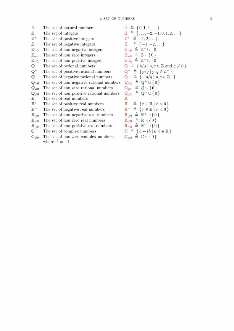
4. SET OF NUMBERS 5

N The set of natural numbers N , { 0, 1, 2, . . . }Z The set of integers Z , { . . . ,�2,�1, 0, 1, 2, . . . }Z+ The set of positive integers Z+ , { 1, 2, . . . }Z� The set of negative integers Z� , {�1,�2, . . . }Z�0 The set of non negative integers Z�0 , Z+ [ { 0 }Z 6=0 The set of non zero integers Z 6=0 , Zr { 0 }Z0 The set of non positive integers Z0 , Z� [ { 0 }Q The set of rational numbers Q , { p/q | p, q 2 Z and q 6= 0 }Q+ The set of positive rational numbers Q+ , { p/q | p, q 2 Z+ }Q� The set of negative rational numbers Q� , {�p/q | p, q 2 Z+ }Q�0 The set of non negative rational numbers Q�0 , Q+ [ { 0 }Q 6=0 The set of non zero rational numbers Q 6=0 , Qr { 0 }Q0 The set of non positive rational numbers Q0 , Q� [ { 0 }R The set of real numbers RR+ The set of positive real numbers R+ , { r 2 R | r > 0 }R� The set of negative real numbers R� , { r 2 R | r < 0 }R�0 The set of non negative real numbers R�0 , R+ [ { 0 }R 6=0 The set of non zero real numbers R 6=0 , Rr { 0 }R0 The set of non positive real numbers R0 , R� [ { 0 }C The set of complex numbers C , { a+ i b | a, b 2 R }C 6=0 The set of non zero complex numbers C 6=0 , Cr { 0 }

where i2 = �1

Part 2

Basics

CHAPTER 2

Logic

1. Motivation

In the first half of 1900s mathematicians believed that entire mathematics can be constructed froma set of axioms, inference rules and symbolic logic. In 1910’s, Bertrand Russell, now known due to hisworks in philosophy, and Alfred North Whitehead published Principia Mathematica which providedcarefully designed construction of mathematics. They claim that every true mathematical statementcan be proved by this way. Unfortunately in 1931 Kurt Godel proved, in his incompleteness theorem,that there are some true statements that cannot be proven if the axiomatic system is consistent andsu�ciently powerful to express the arithmetic of the natural numbers. The famous incompletenesstheorem becomes one of the important milestones in Computer Science, too.

The logic is important for Computer Science in many ways. Search in the web is one of them.When we do search using a search engine in the Internet, we express ourselves using logic. For exampletyping

“Bertrand Russell Mathematica OR Kurt -philosopher”

to Google for search means we are looking pages which contains “Bertrand” and “Russell” wordstogether, either of the words “Mathematica” or “Kurt” but we do not want word “philosopher” inour search. This can be rewritten in logic as “Bertrand” AND “Russell” AND *“Mathematica” OR“Kurt”) AND NOT“philosopher”.

2. Foundations

We use the notation of [TZ82] in defining well-formed logical formula. We use spaces in order toimprove readability as in the case of 8x �(x) or � ^ which should formally be written as 8x�(x) or� ^ .

2.1. Well-formed formula. It is not possible to evaluate an expression such as 2+3+⇥7 sinceit is not properly formed.

Example 2.1. The following expressions are not meaningful. Try to interpret them.i. p ^ q ^ ^ qqii. 1 + + + 1iii. ⇥ / / + � � + 2 3 4iv. 1 2 +v. 1 2 3 ⇥ +

It is correct that these expressions cannot be interpreted in the usual interpretation which is calledinfix notation. Actually the last two can be interpreted in postfix notation as 1 + 2 and 1 + (2 ⇥ 3),respectively. The postfix notation is sometimes called reverse polish notation since it is the reverse ofprefix notation invented by Polish mathematician Jan Lukasiewicz around 1920’s.

Properly formed expressions is the starting point of logic. Formally properly expression is calledwell-formed formula.

The language consists of:Free variables: a0, a1, . . .Bound variables: x0, x1, . . .A predicate symbol: 2Logical symbols: ¬, _ , ^ , �! , ! , 8, 9.Auxiliary symbols: (, ), [, ].�, , ⌘ are meta symbols.

Definition 2.1 (well-formed formula (w↵)).

A formula is well-formed formula (w↵)� ! it is deducible from the following rules:

9

http://en.wikipedia.org/wiki/Bertrand_russell

http://en.wikipedia.org/wiki/Alfred_North_Whitehead

http://en.wikipedia.org/wiki/Principia_Mathematica

http://en.wikipedia.org/wiki/Infix_notation

http://en.wikipedia.org/wiki/Postfix_notation

http://en.wikipedia.org/wiki/Prefix_notation

10 2. LOGIC

i. If a and b are free variables, then [a 2 b] is a w↵.ii. If � and are w↵s, then ¬�, [� _ ], [� ^ ], [� �! ], and [� ! ] are w↵.iii. If � is a w↵ and x is a bound variable, then 8x �(x) and 9x �(x) are w↵, where �(x) is the

formula obtained from the w↵ � by replacing each occurrence of some free variable a by thebound variable x. We call 8x�(x) and 9x�(x) respectively, the formula obtained from � byuniversally , or existentially qualifying on the variable a.

Example 2.2. Examples of w↵s are as follows where p = x0 and q = x1.i. p and q are w↵s due to Definition 2.1(i).ii. ¬p, p _ q, p ^ q, p �! q, p ! q are w↵s due to Definition 2.1(ii).iii. [p ^ q] _ ¬p, [p ^ q] _ ¬[p �! q] are w↵s due to Definition 2.1(i) and (ii) .iv. 9x [x 2 a1] is a w↵. Since

[a0 2 a1] by Definition 2.1(i)9x [x 2 a1] by existential qualifying on a0.

v. 9x [x 2 a1] ^ 8x [x 2 a1] is a w↵.

2.2. Logical Axioms.

Axiom 1 (Logical Axioms).i. � �! [ �! �].ii. [� �! [ �! ⌘]] �! [[� �! ] �! [� �! ⌘]].iii. [¬� �! ¬ ] �! [ �! �].iv. 8x[� �! (x)] �! [� �! 8x (x)] where free variable a on which we are quantifying does

not occur in �.v. 8x�(x) �! �(a) where �(a) is the formula obtained by replacing each occurrence of the bound

variable x in �(x) by the free variable a.

2.3. Rules of Inference.

Axiom 2 (Rules of Inference).i. From � and � �! to infer .ii. From � to infer 8x�(x) where �(x) is obtained from � by replacing each occurrence of some free

variable by x.

Notation.

i. � and � �! =) .ii. � =) 8x�(x).Definition 2.2 (Logically Equivalence).

� is logically equivalent to � ! � is deducible using only the logical axioms. It is denoted by

� ! .

2.4. Equality.

Definition 2.3 (Equality).

a=b� ! 8x [x 2 a ! x 2 b].

Proposition 2.1.i. a = a.ii. a = b �! b = a.iii. a = b ^ b = c �! a = c.

Proof.

i. 8x[x 2 a ! x 2 a].ii. 8x[x 2 a ! x 2 b] =) 8x[x 2 b ! x 2 a].iii. 8x[x 2 a ! x 2 b] ^ 8x[x 2 b ! x 2 c] =) 8x[x 2 a ! x 2 c].

⇤Question 2.1. Do you think that

• NAN = NAN where NAN is “not a number” in programming.• h1

1

i=h11

i

where⇥11⇤is an indeterminate form of limits in Calculus.

3. PROPOSITIONAL LOGIC 11

p f 0=

F

f 1=

p

f 2=

¬p

f 3=

T

F F F T TT F T F T

Table 1. Boolean functions of one variable

p q f 0=

F

f 1=

p^

q

f 2=

¬(p�!

q)

f 3=

p

f 4 f 5=

q

f 6=

p�q

f 7=

p_

q

f 8=

pNORq

f 9=

p !

q

f 10=

¬q

f 11

f 12=

¬p

f 13=

p�!

q

f 14=

pNAND

q

f 15=

T

F F F F F F F F F F T T T T T T T TF T F F F F T T T T F F F F T T T TT F F F T T F F T T F F T T F F T TT T F T F T F T F T F T F T F T F T

Table 2. Boolean functions of two variables

Remark 2.1. If a = b and a w↵ holds for a, then it must hold for b.

a = b =) [�(a) ! �(b)].

3. Propositional Logic

Definition 3.1. A proposition is a statement that is either true or false but not both. The truthvalue of a true proposition is true, denoted by T and that of false proposition is false, denoted by F .

Notation. Propositions are represented by lower case letters such as p, r, q.

3.1. Compound Propositions. We generate new propositions from existing ones by meansof well-formed-formulation. Any w↵ is a generated new proposition based on already establishedpropositions.

Definition 3.2. The set B , {T, F } is called boolean domain where T and F denotes true andfalse, respectively. An n�tuple (p1, p2, . . . , pn) where p

i

2 B is called a boolean n�tuple.

Definition 3.3. An n�operand truth table is a table that assigns a boolean value to all booleann�tuples. A propositional operator is a rule defined by a truth table.

Definition 3.4. An operator is calledmonadicdyadic

if it hasonetwo

operand(s).

Remark 3.1.i. A boolean n�tuple is an element of Bn, that is, (p1, p2, . . . , pn) 2 Bn.ii. There are 2n di↵erent binary n�tuples.iii. A truth table of a predicate p actually defines a function f

p

: Bn ! B.iv. There are 22

ndi↵erent truth tables (functions) of binary n�tuples.

v. There are 221= 4 monadic operators, identity , negation, constant-True, constant-False, as given

in Table 3.1.vi. There are 22

2= 16 dyadic operators as given in Table 3.1.

vii. Note that the functions in the Table 3.1 have interesting properties: Firstly, notice the relationbetween f

i

and the binary representation of i if F and T are represented as 0 and 1, respectively.For example f11 corresponds to TFTT = 1011. Secondly, f

i

= ¬f15�i

as in the case of f3 = ¬f12viii. NAND and NOR are extensively used in logic design in Computer Engineering.ix. p NAND q , ¬(p ^ q). That is, f14(p, q) = ¬f1(p, q).x. p NOR q , ¬(p _ q). That is, f8(p, q) = ¬f7(p, q).

12 2. LOGIC

Definition 3.5. Any w↵ is a compound propositions .

Remark 3.2. In other words, propositions formed from existing propositions using logical opera-tors are called compound propositions .

Definition 3.6. Let p be a proposition. The negation of p, denoted by ¬p or p, is the statement“It is not the case that p”.

Definition 3.7. Let p and q be propositions. The conjunction of p and q, denoted by p ^ q, isthe proposition “p and q”.

p ^ q ,(T, if both p and q are true,

F, otherwise.

Definition 3.8. Let p and q be propositions. The disjunction of p and q, denoted by p _ q, isthe proposition “p or q”.

p _ q ,(F, if both p and q are false,

T, otherwise.

Definition 3.9. Let p and q be propositions.

Theexclusive orconditional statementbiconditional statement

, denoted byp� qp �! qp ! q

, is the functionf6f13f9

in the Table 3.1.

Remark 3.3.i. Conditional p �! q, sometimes called implication.ii. Some other English usages are “if p, then q”, “p implies q” and many more.iii. p is called the hypothesis. q is called the conclusion.

Remark 3.4.i. Biconditional p ! q, sometimes called bi-implication or if-and-only-if , i↵ in short.ii. Some other English usages are “p is necessary and su�cient for q”, “p i↵ q”.iii. Note that p ! q is equivalent to (p �! q) ^ (q �! p).

Definition 3.10. Two compound propositions �(x1, x2, . . . , xn) and (x1, x2, . . . , xn) of the same

variables x1, x2, . . . , xn, are called equivalent� ! they have the same truth tables. It is denoted by

�(x1, x2, . . . , xn) () (x1, x2, . . . , xn),

Remark 3.5. The biconditional, p ! q, is an operator. The equivalence of two compoundpropositions, p () q, is an equivalence relation on the set of all propositions.

Definition 3.11. Let p �! q.

Theconversecontrapositiveinverse

of p �! q isq �! p¬q �! ¬p¬p �! ¬q

.

Corollary 3.1.

Theimplication, p �! qconverse, q �! p

is equivalent tocontrapositive, ¬q �! ¬pinverse, ¬p �! ¬q .

3.2. Application. Logic descriptions is used in all branches of science and engineering. Unam-biguous, precise, consistent reporting is a must.

3.2.1. Translating English sentences. Consider a detective story such as one from Sherlock Holmes.There are people P1, P2, . . . , Pn

. There are corresponding propositions p1, p2, . . . , pn where pi

meansperson P

i

is the murderer. Of course there is a description of the rest of the story which can berepresented as q(p1, p2, . . . , pn). In this formulization if person P3 is the murderer then the truthassignment of (F, F, T, F, . . . , F ) makes q true, that is, q(F, F, T, F, . . . , F ) = T . Here we assume thatthere is one murderer so there is only one entry p

i

= T .3.2.2. System specifications. In engineering precise, formal descriptions are needed. Software de-

velopment is one of them. A typical software life cycle is as follows: A customer who needs a customtailored software solution defines what she wants. This definition will be given to the contractingcompany. The developers start developing the software. At the end the software is delivered to thecostumer. The costumer checks if the developed software meets the specification.

4. PROPOSITIONAL EQUIVALENCE 13

Equivalence Namep ^ T ⌘ p Identity lawsp _ F ⌘ pp ^ F ⌘ F Domination lawsp _ T ⌘ Tp ^ p ⌘ p Idempotent lawsp _ p ⌘ pp ^ q ⌘ q ^ p Commutativity lawsp _ q ⌘ q _ pp ^ (q ^ r) ⌘ (p ^ q) ^ r Associativity lawsp _ (q _ r) ⌘ (p _ q) _ rp ^ (q _ r) ⌘ (p ^ q) _ (p ^ r) Distributivity lawsp _ (q ^ r) ⌘ (p _ q) ^ (p _ r)p ^ (p _ q) ⌘ p Absorption lawsp _ (p ^ q) ⌘ pp ^ ¬p ⌘ F Negation lawsp _ ¬p ⌘ T¬(p ^ q) ⌘ ¬p _ ¬q De Morgan’s laws¬(p _ q) ⌘ ¬p ^ ¬q¬(¬p) ⌘ p Double negation law

Table 3. The laws of logic

In such a scenario the definition should be as precise as possible. Think about the consequences ifthe definition is not precise, informal, possibly ambiguous. It is not that unusual that the definitionshave some conflict or contradicting requirements.

3.2.3. Boolean search. Search in web. It is already mentioned in the motivation that search enginesunderstand the language of predicates.• Translating English sentences• System specifications• Boolean search. Search in web.• Logic puzzles• Logic and bit operations

4. Propositional Equivalence

We use w↵ for compound propositions.

Definition 4.1. A w↵ is called atautologycontradiction

� ! it is alwaystruefalse

independent of the truth

values of its propositions. A w↵ that is neither tautology not contradiction is called a contingency .

Example 4.1. Some simple forms are as follows:Tautologies: T , ¬F , p _ T , p _ ¬p.Contradictions: F , ¬T , p ^ F , p ^ ¬p.Contingencies: p, ¬p, p _ F , p ^ T .

Definition 4.2 (Logically Equivalence).

Two w↵s p and q are called logically equivalent� ! The w↵ p ! q is a tautology. Logically

equivalence of p and q is denoted by p ⌘ q or p () q.

Remark 4.1. Note that logically equivalence is an equivalence relation on the set of all w↵ since:i. Reflexivity: 8p [p () p].ii. Symmetry: 8p, q [(p () q) �! (q () p)].iii. Transitivity: 8p, q, r [(p () q) ^ (q () r) �! (p () r)].

Laws of logically equivalence are given in Table 3.

Example 4.2. T () ¬F , ¬F () p _ T , p _ T () p _ ¬p.

14 2. LOGIC

5. Quantifiers

8x [p(x) _ q(x)](= 8x p(x) _ 8x q(x)8x [p(x) ^ q(x)]() 8x p(x) ^ 8x q(x)9x [p(x) _ q(x)]() 9x p(x) _ 9x q(x)9x [p(x) ^ q(x)] =) 9x p(x) ^ 9x q(x)

Acknowledgment. These notes are based on various books but especially [Ros07, TZ82].

Problems with Solutions

P 2.1. a) Express each of these statements using quantifiers and the following predicateswhere the domain consists of all people.S(x) : x is a student in this class. M(x) : x is a mathematicianL(x) : x likes discrete mathematics course. C(x, y) : x and y are colleaguesK(x, y) : x knows y

i) There are exactly two students in this class who like discrete mathematics course.ii) Every student in this class knows Kurt Godel or knows a mathematician who is a colleagueof Kurt Godel.iii) There is no student in this class who knows everybody else in this class

b) Using rules of inference provide a formal proof forIf 8x [S(x)_Q(x)], and 8x [(¬S(x)^Q(x))! P (x)] are true then 8x [¬P (x)! S(x)] is alsotrue where the domains of all quantifiers are the same.

Solution.

a)i) 9x9y [x 6= y ^ S(x) ^ S(y) ^ L(x) ^ L(y) ^ 8z (S(z) ^ L(z)! z = x _ z = y)]ii) 8x [S(x)! [K(x,Godel) _ 9y (M(y) ^ C(y,Godel) ^K(x, y))]]iii) ¬9x8y [S(x) ^ ((S(y) ^ x 6= y)! K(x, y))]

b)1. 8x [S(x) _Q(x)] Premise2. 8x [(¬S(x) ^Q(x))! P (x)] Premise3. S(a) _Q(a) (1) universal generalization4. (¬S(a) ^Q(a))! P (a) (2) universal generalization5. ¬(¬S(a) ^Q(a)) _ P (a) (4) logical equivalence p! q ⌘ ¬p _ q6. (S(a) _ ¬Q(a)) _ P (a) (5) De Morgan7. (P (a) _ S(a)) _ ¬Q(a) (6) Commutativity and associativity of _8. (P (a) _ S(a)) _ S(a) (7) and (3) resolution9. P (a) _ S(a) (8) Idempotent law10. ¬P (a)! S(a) (9) logical equivalence p! q ⌘ ¬p _ q11. 8x (¬P (x)! S(x)) Universal generalization (a was arbitrary)

CHAPTER 3

Sets, Relations, and Functions

1. Set

1.1. Sets.

Definition 1.1. A set is unordered collection of objects.

Remark 1.1. We do not define set , element , and membership properly. A set is a collection ofelements. Sets are usually represented by capital letters A, B, . . . . Sets are defined either listing of theelements as in A = { a1, a2, . . . }. or those elements that satisfy predicate P (a) as in A = { a | P (a) }.Note that the order of the elements is not important. Due to that unordered n-tuple is represented

as { a1, a2, . . . , an }. If a is an element of A, it is denoted as a 2 A, otherwise as a /2 A.

Example 1.1. The set of natural numbers N = { 0, 1, 2, . . . }. 8 2 N but �3 /2 N.

Example 1.2. E = {x | x 2 N ^ x is even } = {x 2 N | x is even } where the second form is ashort form of the first.

Definition 1.2. The empty set , denoted ;, has no elements in it.

Remark 1.2. There is one and only one empty set. ; has interesting properties: Let A = ; andB = { ; }. Then A 2 B and A ✓ B.

Remark 1.3. Let P (x) be a property. Then the following two propositions are true:i. 8x 2 ; [P (x)]ii. ¬9x 2 ; [P (x)]

Definition 1.3 (Equality of Sets).

A isequalnot equal

to B, denoted byA = BA 6= B

,� ! 8x [x 2 A ! x 2 B ]

9a (a 2 A ^ a /2 B) _ 9b (b /2 A ^ b 2 B).

Example 1.3. { 1, 2, 3 } = { 2, 1, 3 }. Order of elements is not important.

Example 1.4. { 1, 2, 3 } = { 1, 1, 2, 3 }. Repetition of elements is not important.

Example 1.5. x 6= {x }, and {x } 6= { {x } }.Definition 1.4 (Subset).

A is asubsetproper subset

of B, denoted byA ✓ BA ⇢ B

,� ! 8a (a 2 A �! a 2 B)

A ✓ B ^ 9b (b /2 A ^ b 2 B).

Theorem 1.1.Let A be a set.

i. 8A [; ✓ A].ii. 8A [A ✓ A].

Definition 1.5 (Cardinality, Finite Set, Infinite Set). A is finite and n is the cardinality of A� ! There are exactly n distinct elements in A. The cardinality of A is denoted by |A |. A is infinite� ! A is not finite.

Remark 1.4. This definition of infinity needs elaboration.

Example 1.6.0 = | ; |.1 = | { a } | = | { a, a } | = | { ; } | = | { { ; } } | = | { { { ; } } } | = | { { ;, { ; } } } |.2 = | { a, b } | = | { ;, { { ; } } } | = | { ;, { ; } } |.

15

16 3. SETS, RELATIONS, AND FUNCTIONS

Definition 1.6 (Power Set). The power set of A: 2A , {S | S ✓ A }.

Example 1.7. 2{ 1,2,3 } = { ;, { 1 } , { 2 } , { 3 } , { 1, 2 } , { 1, 3 } , { 2, 3 } , { 1, 2, 3 } }.2; = { ; }, 2{ ; } = { ;, { ; } }, 22{ ; }

= { ;, { ; } , { { ; } } , { ;, { ; } } }.

Theorem 1.2. A =S

S22A S.

Theorem 1.3. If A is finite,�� 2A

�� = 2|A |.

Theorem 1.4. 2A = 2B �! A = B.

Proof. By Theorem 1.2, 2A = 2B =)S

S22A S =S

S22B S. Therefore A = B. ⇤Definition 1.7 (Ordered n�tuple). The ordered n�tuple (a1, a2, . . . , an) is the ordered collection

that has ai

as its ith element. (a1, a2) is called ordered pairs . (a1, a2, . . . , an) is equal to (b1, b2, . . . , bn),

denoted by (a1, a2, . . . , an) = (b1, b2, . . . , bn),� ! 8i 2 { 1, . . . , n } a

i

= bi

.

Remark 1.5. An unordered n�tuple is represented by a set. Sets can be used to represent orderedtuples, too. Ordered n�tuple can be represented as sets as:

(a1, a2) , { a1, { a2 } }(a1, a2, a3) , { a1, { a2, { a3 } } }

. . .

Definition 1.8 (Cartesian Product). The cartesian product of A and B is defiend as A⇥B ,{ (a, b) | a 2 A ^ b 2 B }.

Remark 1.6. Note that A ⇥ B 6= B ⇥ A. As an example A = { 1 } and B = { b }. ThenA⇥B = { (1, b) } and B ⇥A = { (b, 1) }. Hence A⇥B 6= B ⇥A.

Theorem 1.5. A⇥ ; = ; ⇥A = ;.

Theorem 1.6. A⇥B = ; �! (A = ; _ B = ;).

Proof. Suppose ¬(A = ; _ B = ;).) A 6= ; ^ B 6= ;.) 9a 2 A ^ 9b 2 B.) (a, b) 2 A⇥B.) A⇥B 6= ;.Hence A = ; _ B = ;. ⇤

Definition 1.9. The Cartesian product of the sets A1, A2, . . . , An

is defined as A1⇥A2⇥ · · ·⇥An

, { (a1, a2, . . . , an) | 8i 2 { 1, . . . , n } ai

2 Ai

}.

Definition 1.10 (Power of a Set An). The nth power of a set , denoted by An, is defined as

A1 = A

An+1 = An ⇥A where n 2 Z+.

1.2. Set Operations.

Definition 1.11 (Union, Intersection).

Theunionintersection

of A and B defined asA [B , {x | x 2 A _ x 2 B }A \B , {x | x 2 A ^ x 2 B } .

Remark 1.7. Set operations can be visualized by Venn diagrams as in Fig. 1

Example 1.8. For sets A,B,C in the figure,A [B = A [ C but B 6= C. &%

'$AkB kC

Definition 1.12. Let C = {A1, A2, . . . , An

} be a collection of sets.

Theunionintersection

of collection C is defined as

Sn

i=1Ai

, A1 [A2 [ · · · [An

= {x | 9i 2 { 1, . . . , n } x 2 Ai

}Tn

i=1Ai

, A1 \A2 \ · · · \An

= {x | 8i 2 { 1, . . . , n } x 2 Ai

}. 1

1. SET 17

(a) Union. (b) Intersection.

(c) Set di↵erence. (d) Symmetric set di↵erence.

Figure 1. Set operations.

Definition 1.13. A and B are disjoint� ! A \B = ;.

Theorem 1.7 (Principle of Inclusion-Exclusion).

|A [B | =(|A |+ |B | if A \B = ;,|A |+ |B |� |A \B | if A \B 6= ;.

Definition 1.14 (Set Di↵erence). The di↵erence ofA andB is defined asArB , {x | x 2 A ^ x /2 B }.

Definition 1.15 (Symmetric Di↵erence). The symmetric di↵erence of A and B is defined as A�B, (A [B)r(A \B).

Definition 1.16 (Complement). The complement of A with respect to the universal set U : A ,U rA.

Theorem 1.8 (Set Identities).Let A,B,C be sets and U be the universal set.A [ ; = A A \ U = A IdentityA [ U = U A \ ; = ; DominationA [A = A A \A = A Idempotent

(A) = A ComplementationA [B = B [A A \B = B \A (Commutativity)A [ (B [ C) = (A [B) [ C A \ (B \ C) = (A \B) \ C (Associativity)A [ (B \ C) = (A [B) \ (A [ C) A \ (B [ C) = (A \B) [ (A \ C) (Distributivity)A [B = A \B A \B = A [B (De Morgan)A [ (A \B) = A A \ (A [B) = A (Absorption)A [A = U A \A = ; (Complement)


Proof of A \ (B [ C) = (A \B) [ (A \ C).A \ (B [ C)= {x | x 2 A \ (B [ C) } definition of membership= {x | x 2 A ^ (x 2 B [ C) } definition of \= {x | x 2 A ^ (x 2 B _ x 2 C) } definition of [= {x | (x 2 A ^ x 2 B) _ (x 2 A ^ x 2 C) } distributivity of ^ over _= {x | (x 2 (A \B) _ (x 2 (A \ C) } definition of \= {x | x 2 (A \B) [ (A \ C) } definition of [= (A \B) [ (A \ C) definition of membership

⇤

2. Relation

Remark 2.1. A⇥B = { (a, b) | a 2 A ^ b 2 B }.

Definition 2.1 (Matrix). An array of numbers with n rows and m columns is called an n ⇥mmatrix . The entry at the ith row and jth column of matrix M is denoted by [M ]

ij

. A matrix withentries 0 and 1 only is called a binary matrix . Binary matrices are also called (0, 1)�matrices.

Definition 2.2. ↵ is called a binary relation from A to B� ! ↵ ✓ A ⇥ B. We use the infix

notation of a↵ b whenever (a, b) 2 ↵.

Remark 2.2. If sets A and B are finite with |A| = n and |B| = m, the elements of A and Bcan be listed in an arbitrary order as A = { a1, a2, . . . , an } and B = { b1, b2, . . . , bm }. Then binaryrelation ↵ ✓ A⇥B can be represented by an n⇥m (0, 1)�matrix, denoted by M

↵

, as

[M↵

]ij

,(1, a

i

↵ bj

0, otherwise.

Note that there are n rows correspond to the ordered elements of A, and m columns correspondto the ordered elements of B.

Example 2.1.Let ↵ = { (3, b), (3, c), (7, c) } ✓ A⇥B where A = { 1, 3, 7 } and B = { a, b, c, d }.

Using the orderings ofA = { 1, 3, 7 } and B = { a, b, c, d } we have

M↵

=

a b c d137

2

40 0 0 00 1 1 00 0 1 0

3

5

Using a di↵erent orderings such asA = { 7, 1, 3 } and B = { c, a, d, b } the matrixchanges to

M↵

=

c a d b713

2

41 0 0 00 0 0 01 0 0 1

3

5.

2. RELATION 19

Remark 2.3. The cartesian and the matrix representations are related. Rotate the cartesianrepresentation by 90� clockwise, and compare with the matrix representation.

Question 2.1. How many di↵erent binary relations from A to B can be defined?

2.1. Composition of Relations.

Definition 2.3 (Composition of Relations).Let ↵ ✓ A ⇥ B,� ✓ B ⇥ C. The composition of ↵ and �, denoted by ↵ � �, is defined as ↵ � � ,{ (a, c) 2 A⇥ C | 9b 2 B [a↵ b ^ b� c] }.

Remark 2.4. Note that ↵ � � ✓ A ⇥ C. Note that this notation of composition is di↵erent thatthe notation of composition of functions which will be discussed at Sec. 3.

Definition 2.4 (Boolean Matrix Multiplication).Let M

↵

and M�

be n⇥m and m⇥ p binary matrices. The binary product of M�

and M↵

, denoted byM

↵

�M�

, is an n⇥ p binary matrix defined as

[M↵

�M�

]ij

,(1, 9k [1 k m ^ [M

↵

]ik

= 1 ^ [M�

]kj

= 1]

0, otherwise.

Remark 2.5. Binary matrix multiplication can be defined by means of logic functions.

[M↵

�M�

]ij

=m_

k=1

[M↵

]ik

^ [M�

]kj

where ^ and _ are logical AND and OR functions. The notationW

m

k=1, is similar toP

m

k=1, is definedasW

n

k=1 , p1 _ p2 _ · · · _ pn

.

Example 2.2. Using orders A = { 1, 2 }, B = { a, b, c } and C = {A,B,C,D }:

1 1 00 1 0

��

2

41 1 1 00 1 1 01 0 0 1

3

5 =

1 1 1 00 1 1 0

�

M↵

� M�

= M↵��

But regular matrix multiplication gives:1 1 00 1 0

�⇥

2

41 1 1 00 1 1 01 0 0 1

3

5 =

1 2 2 00 1 1 0

�

M↵

⇥ M�

= M↵

⇥M�

.

Theorem 2.1. M↵�� = M

↵

�M�

.

Theorem 2.2 (Associativity).(↵ � �) � � = ↵ � (� � �) whenever (↵ � �) � � is defined.

Corollary 2.3 (Associativity).M

↵

� (M�

�M�

) = (M↵

�M�

)�M�

whenever M↵

� (M�

�M�

) is defined.


Definition 2.5 (Inverse of a Binary Relation). The inverse of a binary relation, denoted by ↵�1,

is defined as b↵�1 a� ! a ↵ b.

Definition 2.6. The transpose of a matrix, denoted by M>, is defined as [M>]ij

, [M ]ji

.

Theorem 2.4. M↵

�1 = (M↵

)>.

Theorem 2.5. [↵ � �]�1 = ��1 � ↵�1.

Definition 2.7. The complement of ↵, denoted as ↵, is defined as a↵ b� ! ¬ a↵ b.

Theorem 2.6. M↵

= 1�M↵

where 1 is matrix of all 1s.

Example 2.3. Show that (↵)�1 = (↵�1)(a, b) 2 (↵)�1 , (b, a) 2 ↵, (b, a) /2 ↵, (a, b) /2 ↵�1 , (a, b) 2 (↵�1).

3. Functions

Remark 3.1. Let f be a relation from A to B. Pick an a 2 A and consider the corresponding setB

a

✓ B defined as Ba

, { b | (a, b) 2 f }. Note that |Ba

| could be 0, 1, 2, . . . .

If |Ba

| =01n � 2

, then a isnot mapped to any b 2 Bmapped to exactly one b 2 Bmapped to n elements of B

.

Definition 3.1. A relation f ✓ A⇥B is called partial function� ! 8a 2 A |B

a

| 1.

Remark 3.2. Any computer program is actually a partial function from its input space to itsoutput space. For some inputs in its domain it terminates and produces outputs. For some otherinputs it does not terminate. Hence for those inputs there is no corresponding outputs. That is thereason that it is a partial function.

Definition 3.2. A relation f ✓ A⇥B is called function� ! 8a 2 A |B

a

| = 1.

Example 3.1. Remember function y = f(x) = 1x�1 from Calculus. It is considered to be a func-

tion from R to R. Properly speaking this statement is not true since it is not defined at x = 1 2 R.

-5 -4 -3 -2 -1 0 1 2 3 4 5

-3

-2

-1

1

2

3

Actually, it is a function from Rr { 1 } to R. On the other hand, it is a partial function from R to R.

Definition 3.3.ABf(A)

is called thedomaincodomainrange

of f and written asdom fcod fran f

.

Question 3.1. Consider the ceiling function f(x) = dx e. dom f = ?, cod f = ?, ran f = ?

Notation.

• b = f(a)� ! a f b

• A function f from A to B is represented by f : A! B.• The set all functions from A to B is represented by BA.• f(C) = { f(c) | c 2 C } for C ✓ A.

Remark 3.3.

LetBA

PR

be the set of allfunctionspartial functionsrelations

from A to B. Then BA ✓ P ✓ R.

3. FUNCTIONS 21

Question 3.2.

•��BA

�� =?• | P | =?• |R | =?

Theorem 3.1. If A and B are finite sets, not both empty, then��BA

�� = |B ||A |.

Question 3.3. Let A be a nonempty set.

•�� ;A

�� = ?

•��A; �� = ?

•�� ;;

�� = ?

Definition 3.4. Let f : A! B and AS

✓ A ✓ AL

.Function f

S

✓ AS

⇥B is the restriction of f to AS

� ! [8a 2 A, 8b 2 B ((a, b) 2 fS

! (a, b) 2 f)].Then partial function f

L

✓ AL

⇥B is an extension of f to AL

� ! [8a 2 A1, 8b 2 B ((a, b) 2 fL

! (a, b) 2 f)].

Remark 3.4 (The inverse of a function). Note that for any relation ↵ from A to B, there is aunique inverse relation from B to A. This inverse relation usually denoted by ↵�1. Since a function ffrom A to B is also a relation, there is an inverse relation from B to A which is also denoted as f�1.Note that f�1 is a relation but not necessarily a function. f�1 becomes a function if and only if f isa bijection.

Definition 3.5. Let f : A! B.

f is called

the identitya surjectionan injectiona bijectiona permutation

� !

A = B ^ 8a 2 A f(a) = af(A) = B8a1, a2 2 A [a1 6= a2 ! f(a1) 6= f(a2)]surjection ^ injectionf : A! A and f is a bijection

.

Theorem 3.2. Let f : A ! B and g : B ! C be functions If f and g aresurjectionsinjectionsbijections

, then

g � f is alsoa surjectionan injectiona bijection

.

Remark 3.5 (Composition of functions). The notations of composition of relations and composi-tion of functions are unfortunately inconsistent. Let f : A! B and g : B ! C. Then the compositionof function f with function g is represented by g � f . On the other hand, the composition of relationf with relation g is f � g. Although we end up with two di↵erent expressions, they actually representthe same set

{(a, c) 2 A⇥ C | a 2 A, c 2 C, 9b 2 B ((a, b) 2 A⇥B ^ (b, c) 2 B ⇥ C)}.When f and g are functions, we always use functional interpretation and notation.

Functional interpretations. In traditional notation for functions, we have b = f(a) and c =g(b). Hence c = g(b) = g(f(a)) = (g � f)(a).

Relational interpretations. Since functions are special relations, we can apply composition ofrelations to these special relations. Then functions f and g are also two relations. So in relationnotation, we have afb and bgc. Then f � g is the composition of relation f with relation g. Note thatf � g is relation from A to C. Hence we have a(f � g)c.

This inconsistency in notation is probably due to the convenience of matrix representations inthe composition of relations. Remember that M

↵�� = M↵

�M�

where M↵�� is the matrix of the

composition of ↵ with �. A formula such as M��↵ = M

↵

�M�

would not be that convenient.

Theorem 3.3. Let f : A ! B and g : B ! C be functions. Then the composition of functionsg � f is a function: g � f : A! C where (g � f)(a) = g(f(a)).


Remark 3.6.

• If functions f : A! B and g : B ! C are invertible, then the function g �f is also invertibleand (g � f)�1 = f�1 � g�1.

• f�1(B) = { a 2 A | f(a) 2 B }• Let f : R! R. Then f and f�1 are symmetric with respect to y = x line.

Example 3.2.Show that any function f : A ! B can be represented as the composition of functions g and h,f = h � g, where g is a surjection, h is an injection.

DefineD = {Di

✓ A | d1, d2 2 Di

, f(d1) = f(d2) }.Define g : A! D 3 g(a) = D

i

= f�1(f(a)).Then, clearly g is a surjection since 8D

i

2D⇥9a 2 A

⇥D

i

= f�1(f(a))⇤⇤, hence g(a) = D

i

.Define h : D ! B 3 h(D

i

) = h(f�1(f(a))) =f(a).Let D

i

6= Dj

. Then, for di

2 Di

and dj

2 Dj

,f(d

i

) 6= f(dj

). So h(Di

) 6= h(Dj

). Therefore, h isan injection.

(h � g)(a) = h(g(a)) = h(f�1(f(a))) = f(a)So, h � g = f .

Question 3.4.• Are D

i

’s disjoint?• What is f�1(B)?• What is f(f�1(B))?• What kind of function is f if B\f(A) = ;?• What kind of function is f if 8b 2 B

⇥�� f�1(b)�� = 1

⇤?

• If |A | = n, |B | = n, what is the number di↵erent functions f ?

Remark 3.7. Let f : A ! B be a function and A and B be finite sets. If f isan injectiona surjectiona bijection

.

then|A | |B ||A | � |B ||A | = |B |

.

For functions from a set to itself has an interesting property that it can be applied repeatedly. Letf : A! A be a function and a 2 A. Then f(a), f(f(a)), . . . , f(f(f(a))), . . . are all defined.

Definition 3.6 (Power of a function). Let f : A ! A be a function. Power of a function isdefined as

i. f1 , f .ii. fn+1 , f � fn for n 2 Z+.

Definition 3.7 (fixed point). Let f : A ! A be a function. a 2 A is called a fixed point of f� ! f(a) = a,

PROBLEMS WITH SOLUTIONS 23

Remark 3.8. Fixed points are important in Computer Science. If a is a fixed point of f thenfn(a) = a for all n 2 N.

Question 3.5. Consider functions from R to R. Let a, b, c 2 R.• What are the fixed points of f(x) = ax+ b where a and b are real parameters? Consider the caseswhere a = 1 and b = 1, a = 2 and b = 1, and a = 1 and b = 0.

• What are the fixed points of f(x) = ax2 + bx + c where a, b and c are real parameters? Considerthe cases for di↵erent values of a, b and c.

• What are the fixed points of f(x) = sinx?• The function f(x) = rx(1 � x) from Z to Z is called the logistics map where r 2 R is a parame-ter [Str94]. Although it seems simple logistic map has unexpectedly rich properties if it is appliediteratively, i.e. x

n+1 = rxn

(1�xn

). Try to plot logistic map for r = 2.8, r = 3.3, r = 3.5, r = 3.857.

Acknowledgment. These notes are based on various books but especially [PY73, Ros07,TZ82, Gal89, Hol60, Nes09].


P 3.1. a) Prove or disprove that set di↵erence distributes over union, that is,

A� (B [ C) = (A�B) [ (A� C).

b) Given a nonempty set A, let f : A! A and g : A! A where

8a 2 A f(a) = g(f(f(a))) and g(a) = f(g(f(a)))

Prove that f = g.

Solution.

a) A� (B [ C) = (A�B) [ (A� C)Consider the following counter example which disproves the statement.Let A = {1, 2, 4, 5}, B = {2, 3, 5, 6} and C = {4, 5, 6, 7}.Then A� (B [ C) = {1, 2, 4, 5}� {2, 3, 4, 5, 6, 7} = {1} and(A�B) [ (A� C) = ({1, 2, 4, 5}� {2, 3, 5, 6}) [ ({1, 2, 4, 5}� {4, 5, 6, 7}) = {1, 2, 4}.Hence, A� (B [ C) 6= (A�B) [ (A� C).

b) Proof by contradiction: Let f : A! A and g : A! A and8a 2 A f(a) = g(f(f(a))) (I), and g(a) = f(g(f(a))) (II), but f 6= g.Then 9s 2 A f(s) 6= g(s).

f(s) 6= g(s), g(f(f(s))) 6= g(s) since f = g(f(f)), f(g(f(f(f(s))))) 6= g(s) since g = f(g(f)), f(g(f(f| {z }

f

(f(s))))) 6= g(s)

, f(f(f(s))) 6= g(s) since f = g(f(f)), f(f( f|{z}

g(f(f(s)))

))) 6= g(s)

, f(f(g(f(f(s))))) 6= g(s) since f = g(f(f)), f(f(g(f| {z }

g

(f(s))))) 6= g(s)

, f(g(f(s))) 6= g(s) since g = f(g(f)), g(s) 6= g(s) since g = f(g(f)). Contradiction!Hence, f = g.

CHAPTER 4

Relations on a Set

1. Relations on a Set

Definition 1.1. Let ⇢ be a relation on A, that is ⇢ ✓ A⇥A.

⇢ is called


� !

8a 2 A [a ⇢ a]8a, b 2 A [a ⇢ b �! b ⇢ a]8a, b 2 A [a ⇢ b ^ b ⇢ a �! a = b]8a, b, c 2 A [a ⇢ b ^ b ⇢ c �! a ⇢ c]

Theorem 1.1. If ⇢ is


then ⇢�1 is


.

Example 1.1.

a

�� b

��

c

d e

2

66664

0 1 1 0 00 0 0 1 10 0 0 0 00 0 0 0 00 0 0 0 0

3

77775A treeRST

1 4oo

�� ✏✏2

OO

3oo

^^

2

664

0 0 0 01 0 0 01 1 0 01 1 1 0

3

775 greater then relationRST

•1↵1)) •2

↵7))

↵3

ii •3↵9

ii

2

40 1 01 0 10 1 0

3

5 a↵b� ! | a� b | = 1

RST

2. Observations on the Matrix of a Relation

Let ↵ ✓ A⇥A.

• ↵ is ordinary �! No pattern in the matrix.2

664

1 1 0 00 0 1 01 0 0 11 0 1 0

3

775

• '' •��

Use directed graph.• ↵ is reflexive ! The main diagonal is all 1’s.2

664

1 1 0 00 1 1 01 0 1 11 0 1 1

3

775

•a��⌘ •

Omit loops.

25

26 4. RELATIONS ON A SET

• ↵ is symmetric ! The matrix is symmetric.2

664

1 1 0 01 0 1 00 1 1 00 0 0 1

3

775

2

664

1 . . .1 0 . .0 1 1 .0 0 0 1

3

775

• '' •gg ⌘ • •

Use undirected graph.• ↵ is both reflexive and symmetric.2

664

1 0 1 00 1 1 01 1 1 10 0 1 1

3

775

2

664

. . . .0 . . .1 1 . .0 0 1 .

3

775

• ''⌘⌘•gg��⌘ • •

• ↵ is transitive.

•

((

((•

•

VV

3. Closure of Relations

Example 3.1. Given a relation ↵0 which is not reflexive, a new relation ↵1 can be defined whichis reflexive and ↵0 ✓ ↵1. More than that, there are many reflexive relations ↵

j

with ↵0 ✓ ↵j

. Notethat ↵1 is the smallest one satisfying this.

↵0 =

2

664

1 1 0 00 1 1 01 0 1 11 0 1 0

3

775 ↵1 =

2

664

1 1 0 00 1 1 01 0 1 11 0 1 1

3

775 ↵2 =

2

664

1 1 1 00 1 1 01 0 1 11 0 1 1

3

775

Definition 3.1. Let ↵ be a relation on a set A. Let P be a property such as reflexivity, symmetry,

transitivity. � is called closure of ↵ with respect to P� ! � is a relation with property P and ↵ ✓ �

with 8� [↵ ✓ �] where � is a relation with property P and � ✓ �

Remark 3.1. Note that � is the smallest relation satisfying this.

4. Compatibility Relation

Let � ✓ A⇥A.

Definition 4.1 (Compatibility Relation).

A relation � is a compatibility relation� !

i. � is reflexiveii. � is symmetric

Remark 4.1. Note that equivalence relation has one more property, namely transitivity.� is an equivalence relation �! � is a compatibility relation.

Definition 4.2. C ✓ A is called a compatibility class (compatible)� !

8c1, c2 2 C [c1 � c2] where � is a compatibility relation.

Definition 4.3. A compatibility class which is not properly contained in any other compatibilityclass is called a maximal compatibility class (maximal compatible).

Definition 4.4. A complete cover , C�

(A), of A with respect to � is a collection of all and onlythe maximal compatibles induced by �.� ! A collection, C

�

(A), of all and only the maximal compatibles induced by � on A is called acomplete cover of A.

5. EQUIVALENCE RELATION 27

Theorem 4.1. If � is compatibility relation on a finite set A and C is a compatibility class, thenthere is a maximal compatibility class C

0such that C ✓ C

0.

Theorem 4.2. There is a one-to-one correspondence between � and C�

(A).

Theorem 4.3. � is a compatibility relation on A� ! 9 relation ⇢ from A to some B 3 � = ⇢⇢�1

with 8a 2 A [9b 2 B [a ⇢ b]]

Example 4.1.

Complete coverC�

(A) = {A1, A2, A3, A4, A5, A6} is a complete cover.C

0�

(A) = {A1, A2, A3, A4, A5, A7} is not since A4 ✓ A7.

4.1. Application of Compatibility Relation.

Example 4.2 (Minimization of Incompletely Specified Finite State Machines). S = { a, b, c, d, e }I1 I2 I3

a c,0 e,1 -b c,0 e,- -c b,- c,0 a,-d b,0 c,- e,-e - e,0 a,-

Definition 4.5. States a and b are compatible, a�b, where � ✓ S⇥S� ! If no applicable input

sequence to both a and b produce conflicting outputs.

� is a compatibility relation since 8a, b 2 Si. a�a.ii. a�b �! b�a.

ap

b c,c e,ep

c ⇥ b,c c,ep

d b,c c,e b,c c,e ⇥p

e ⇥ e,e c,e a,a ⇥p

a b c d e

{ a, b } is a compatible.{ a, b, d } is a maximal compatible.{ { a, b, d } , { b, c, e } } is a complete cover.

Let A = { a, b, d } , B = { b, c, e }I1 I2 I3

A B,0 B,1 B,-B B,0 B,0 A,-

5. Equivalence Relation

Definition 5.1 (Equivalence Relation).

A relation � is a equivalence relation� !

i. � is reflexive


ii. � is symmetriciii. � is transitive

Theorem 5.1. If � is an equivalence relation �! � is also a compatibility relation.

Definition 5.2 (Equivalence Class).A maximal compatible of � is called an equivalence class where � is an equivalence relation.

Theorem 5.2. Let {Ei

} be complete cover. 8E1, E2 2 C�

(A) [Ei

\ Ej

= ;]

Theorem 5.3. 8a 2 A [a belongs to one and only one equivalence class].

Definition 5.3 (Partition).

A set P = {Ai

6= ; | Ai

✓ A } is called a partition of A� !

i.S

i

Ai

= Aii. A

i

\Aj

= ; if i 6= j.

Each Ai

is called a block of P .

P is called the partition of singletons� ! 8A

i

2 P [|Ai

| = 1].The partition of singletons and the partition {A } are called the trivial partitions.

Example 5.1. Let A = { 1, 2, 3, 4, 5 }. Then sets P1 = { { 1 } , { 2 } , { 3 } , { 4 } , { 5 } }, P2 ={ { 1 } , { 2, 3, 4, 5 } }, P3 = { { 1 } , { 2, 4, 5 } , { 3 } }, P4 = { { 1, 2 } , { 3, 5 } , { 4 } }, P5 = { { 1, 2, 3, 4, 5 } }are partitions of A.Note that P1 and P5 are the trivial partitions.

Theorem 5.4. There is a one-to-one corresponding between equivalence relations on A and parti-tions on A.

Definition 5.4. Dichotomy is a partition with two blocks.

Theorem 5.5. � is an equivalence relation on A ! 9B⇥9f : A! B

⇥� = ff�1

⇤⇤.

P = {A1, A2, A3, A4 }.

Theorem 5.6. Let ↵ and � be equivalence relations on A.↵ � is an equivalence relation ! ↵� = �↵

Proof.

() part:) ↵� is an equivalence relation �! ↵� is symmetric �! ↵� = (↵�)�1 = ��1↵�1 = �↵.Since ↵ and � are symmetric.(( part:)

i. 8a 2 A [a↵a ^ a�a] �! a↵�a. reflexivity.ii. 8a, b 2 A a(↵�)b �! a(�↵)b �! 9d 2 A [a�d ^ d↵b] �! d�a ^ b↵d �! b(↵�)a.

symmetry.iii. Left as an exercise. ⇤

5.1. Applications of Equivalence Relations. An application of equivalence relations is statereduction of a completely specified FSM.

Definition 5.5. A finite state machine (FSM ) is a system M = [Q,S,R,↵,� ] whereQ is a finite set of statesS is a finite set of input symbols (input of alphabet, stimulus)R is a finite set of output symbols (output alphabet, response)↵ : Q⇥ S ! Q is the state function� : Q⇥ S ! R is the output function


Example 5.2 (State Reduction of a Completely Specified Finite State Machine).Let FSM be defined as: Q = { a, b, c, d, e, f, g, h } S = { I1, I2 } R = { 0, 1 } and ↵ and � are defined inthe following table:

↵,� I1 I2a b, 1 h, 1b f, 1 d, 1c d, 0 e, 1d c, 0 f, 1e d, 1 c, 1f c, 1 c, 1g c, 1 d, 1h c, 0 a, 1

Define ⌘✓ Q⇥Q as follows:a is equivalent to b ! a ⌘ b� ! no input sequence can distinguish a from b.

⌘ is an equivalence relationsince 8a, b, c 2 S

i. a ⌘ aii. a ⌘ b �! b ⌘ aiii. a ⌘ b, b ⌘ c �! a ⌘ c

a

b

b,fd,h

c

d

c,de,f

e

b,dc,h

d,fc,d

f

b,cc,h

c,fc,d

c,dc,c

g

b,cd,h

c,fd,d

c,dc,d

c,cc,d

h

c,da,e

c,ca,f

a b c d e f g h

f e

d

c

ba

h

g

complete cover:{ { a } , { b } , { c, d } , { e, f, g } , {h } }

Let A = { a } , B = { b } , C = { c, d } , E = { e, f, g } , H = {h }I1 I2

A B,1 H,1B E,1 C,1C C,0 E,1E C,0 C,1H C,1 A,1

Acknowledgment. These notes are based on various books but especially [PY73, Ros07,TZ82, Gal89]. Class of CMPE220 of Fall 2008 did the initial LATEX draft of hand written notes.


P 4.1. Let ⇢ ✓ A⇥A, ⇢�1 be the inverse relation of ⇢, and iA

be the identity relation of A. Whatkind of relation is ⇢ if


i) iA

✓ ⇢.ii) i

A

\ ⇢ = ; .iii) ⇢�1 = ⇢.iv) ⇢ \ ⇢�1 ✓ i

A

.v) ⇢ \ ⇢�1 = ;.vi) ⇢ = [

i2N ⇢i.Justify your answers.Solution.

If

iA

✓ ⇢iA

\ ⇢ = ;⇢�1 = ⇢.⇢ \ ⇢�1 ✓ i

A

.⇢ \ ⇢�1 = ;.⇢ = [

i2N ⇢i.

, then ⇢ is

reflexiveirreflexivesymmetricantisymetricasymmetrictransitive

.

Justification is left as exercise.

CHAPTER 5

Partial Ordering, Lattice

1. Partial Ordering

Definition 1.1. Let be a relation on A, ✓ A⇥A.

is a Partial Ordering� !

i. reflexiveii. antisymmetriciii. transitive.

a < b� ! a b ^ a 6= b.

Theorem 1.1. The inverse relation �1 of a partial ordering is also a partial ordering, denotedby �.

Theorem 1.2. The directed graph of a partial ordering relation contains no circuits of lengthgreater than 1.

Definition 1.2 (Poset).A partly ordered set (poset), denoted [A, ], consists of a set A and a partial ordering relation onA.

Definition 1.3. Let [A, ] be a poset. a, b 2 A are said to be comparable� ! a b _ b a.

a, b 2 A are incomparable� ! a, b 2 A are not comparable.

Definition 1.4 (Linearly ordered set). [A, ] is called a linearly ordered set� ! 8a, b 2

A [a b _ b a].

Remark 1.1. Note that some elements of a poset are incomparable but every two elements in atotally ordered set should be comparable.

Example 1.1.

a b

c

@@ 77

d

^^

e

__ ??

f

OO

g

^^

Let A = { a, b, c, d, e, f, g } and b a repre-sented by b! a.

Note that c a, f a. There should be anarc from f to a, too. In order to simplify thefigure this kind of arcs are omitted.

a and b are not comparable. So there is noelement that is larger than all the other elements.Similarly there is no element that is smaller thanall the other elements.

Definition 1.5 (Consistent Enumeration).A consistent enumeration of a finite poset A is a function i : A! N such that8a

p

, aq

2 A [ap

aq

�! i(ap

) i(aq

)].

Theorem 1.3. Every finite poset admits of a consistent enumeration.

Example 1.2.

A = { a, b }2A = { ;, { a } , { b } , { a, b } }

[P (A),✓ ] is a poset.

31

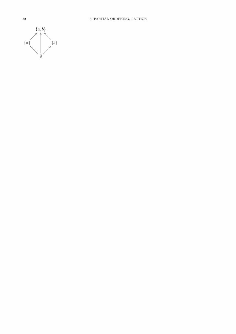
32 5. PARTIAL ORDERING, LATTICE

{a, b}

{b}

__

{a}

??

;

OO

__ ??

2. HASSE DIAGRAM 33

2. Hasse Diagram

Definition 2.1. Let [A, ] be a poset and a, b 2 A with a 6= b. a is an immediate predecessor of

b, denoted by a � b,� ! a < b and @c 2 A [a < c < b].

b is an immediate successor of a, denoted by b � a,� ! a < b and @c 2 A [a < c < b].

Remark 2.1.

i. As convention an upper element is larger than a lower element.ii. Immediate predecessor relation is

• not reflexive• not symmetric• not transitive

iii. Given an immediate predecessor relation one can obtain the corresponding partial ordering.iv. covers �.v. Immediate relation simplifies the graph of partial ordering relation.

Definition 2.2. The graph of � is called Hasse Diagram.

Example 2.1. Reflexive+Symmetric+Transitive

a��

b

__

↵↵c

??

11

d

OO

__ ??

11

RST

a

b

__

c

??

d

OO

__ ??

RST

a

b

__

c

??

d

__ ??

RST

Example 2.2.a | b � ! 9c 2 Z [b = ca]

Let A = { a 2 N | a | 100 } and define a relation on A as a b� ! a | b.

100��

20��

==

50��

aa

4��

??

44

10��

aa ==

OO

25��

aa

jj

2��

__ ==

OO

MM

MM

5��

aa >>

OO

QQ

QQ

1��

aa ==

QQ MM

PP NN

EE

]]

Graph of

100

20 50

4 10 25

2 5

1

Graph of �• not reflexive• not symmetric• not transitive

Hasse diagram.


3. Lattice

Definition 3.1. Let [A, ] be a poset.

m 2 A ismaximalminimal

� ! @a 2 A [m < a]@a 2 A [a < m]

.

Definition 3.2. Let [A, ] be a poset and B ✓ A.

s 2 A is called a supremum of set B� !

i. 8b 2 B b s.ii. @a 2 A 8b 2 B b a �! a < s.

Question 3.1. Define infimum of B.

Remark 3.1. Consider intervals X = [0, 1] and Y = (0, 1) of the real numbers R. Then 0 and 1are minimal and maximal of X, respectively. Since 0 /2 Y , 0 cannot be a minimal of Y . 0 is a infimumof Y . 1 is a supremum of Y . Since R is totally ordered, there is no other infimum than 0. So we cansay that 0 is the infimum of Y . Similarly 1 is the supremum of Y .

Definition 3.3. Let [A, ] be a poset and I,O 2 A.IO

is thegreatestleast

� ! 8a 2 A [a I]8a 2 A [O a]

. I and O are called universal upper bound and universal

lower bound , respectively.

Remark 3.2.• From now on all posets are finite.• If poset is finite, there are minimal and maximal elements but there may not be universal upperand lower bounds.

Example 3.1.

a b

c

d e f

g h

i

j k

maximals: a, b, h.minimals: d,g,j,k.greatest: none.least: none.

3. LATTICE 35

Definition 3.4. Let [A, ] be a poset and a, b 2 A.A least upper bound (lub) of a and b is c 2 A

i. a c and b cii. @x 2 A [a x ^ b x ^ x < c]

Remark 3.3. Let a, b 2 A.i. Least upper bound of a and b may not exist.ii. There may be more than one lub.iii. It may be unique. If lub of a and b is unique, then it is denoted as a+ b.

Theorem 3.1. 8a, b 2 A [ lub exists] �! [A, ] has the universal upper bound I.

Example 3.2.

a b

c d

e

f

• There is no universal upper bound.• a and b are maximal elements.• a and b are lub of c and d.• e and f are lower bounds of c and d.• e is unique glb of c and d.• f is the universal lower bound O.


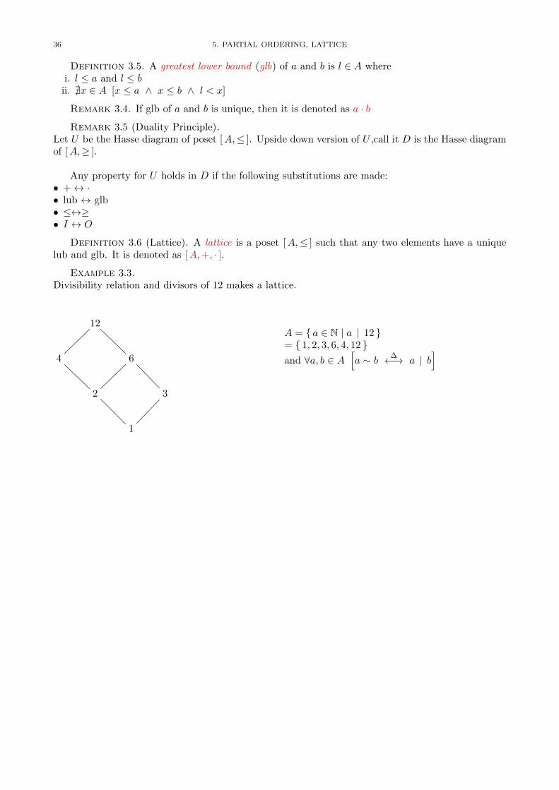
Definition 3.5. A greatest lower bound (glb) of a and b is l 2 A wherei. l a and l bii. @x 2 A [x a ^ x b ^ l < x]

Remark 3.4. If glb of a and b is unique, then it is denoted as a · b

Remark 3.5 (Duality Principle).Let U be the Hasse diagram of poset [A, ]. Upside down version of U ,call it D is the Hasse diagramof [A,� ].

Any property for U holds in D if the following substitutions are made:• +$ ·• lub $ glb• $�• I $ O

Definition 3.6 (Lattice). A lattice is a poset [A, ] such that any two elements have a uniquelub and glb. It is denoted as [A,+, · ].

Example 3.3.Divisibility relation and divisors of 12 makes a lattice.

12

4 6

2 3

1

A = { a 2 N | a | 12 }= { 1, 2, 3, 6, 4, 12 }and 8a, b 2 A

ha ⇠ b

� ! a | bi


Theorem 3.2. Let [A,+, · ] be a lattice and a, b, c 2 A.i. a+ a = a idempotencyii. a+ b = b+ a commutativityiii. (a+ b) + c = a+ (b+ c) associativityiv. a+ (a · b) = a absorptionv. a+ b = b ! a · b = a ! a b consistency

4. Applications

• PageRank of Google.• Measure the similarity of two orderings (ranking) on a set, i.e. Pearson correlation.

Acknowledgment. These notes are based on various books but especially [PY73, Ros07,Gal89].


P 5.1.

Definition 4.1. Let f, g : Z+ ! R. g dominates f� ! 9m 2 R+ and 9k 2 Z+ such that

|f(n)| m |g(n)| for all n 2 Z+ where n � k

Definition 4.2. For f : Z+ ! R, f is big Theta of g, denoted by f 2 ⇥(g),� ! there exist

constants m1,m2 2 R+ and k 2 Z+ such that m1|g(n)| |f(n)| m2|g(n)|, for all n 2 Z+, wheren � k.a) Let RZ+

be the set of all functions from Z+ to R.Define the relation � on RZ+

as

f�g� ! f 2 ⇥(g) for f, g 2 RZ+

.

Prove that � is an equivalence relation on RZ+.

b) Let [f ]�

represent the equivalence class of f 2 RZ+for the relation �. Let E be the set of

equivalence classes induced by �. Define the relation ↵ on E by

[f ]�

↵ [g]�

, for f, g 2 RZ+,

� ! f is dominated by g.

Show that ↵ is a partial order.Use shorthand notations F for RZ+

and [f ] for [f ]�

.

Solution.

a) We need to show that � is reflexive, symmetric and transitive.i. For each f 2 F , |f(n)| 1 |f(n)| for all n � 1. So f�f , and � is reflexive.ii. For f, g 2 F ,

f�g ) f 2 ⇥(g)

) mf

|g(n)| |f(n)| Mf

|g(n)| for n � k where mf

,Mf

2 R+ and k 2 Z+

) |g(n)| 1/mf

|f(n)| and 1/Mf

|f(n)| |g(n)|) m

g

|f(n)| |g(n)| Mg

|f(n)| for n � k with mg

= 1/Mf

,Mg

= 1/mf

2 R+

) g 2 ⇥(f)

) g�f.

So � is symmetric.iii. Let f, g, h 2 F with f�g, g�h. Then, f 2 ⇥(g) and g 2 ⇥(h) ) for all n 2 Z+, there exist

constants mf

,Mf

,mg

,Mg

2 R+ and kf

, kg

2 Z+ such thatm

f

|g(n)| |f(n)| Mf

|g(n)| for n � kf

, andm

g

|h(n)| |g(n)| Mg

|h(n)| for n � kg

. Then for n � max{kf

, kg

},m

f

mg

|h(n)| mf

|g(n)| |f(n)| and|f(n)| M

f

|g(n)| Mf

Mg

|h(n)|. Hence for n � k,m |h(n)| |f(n)| M |h(n)|


where m = mf

mg

,M = Mf

Mg

2 R+ and k = max{kf

, kg

} 2 Z+. So f�h, that is, �transitive.

b) We need to show that ↵ is reflexive, antisymmetric and transitive. Let f, g, h 2 RZ+.

i. f is dominated by f since |f(n)| |f(n)| for n � 1. So [f ]↵[f ], hence ↵ is reflexive.ii. Suppose [f ]↵[g] and [g]↵[f ]. Then

|f(n)| mf

|g(n)| for n � kf

for some mf

and kf

. Similarly,|g(n)| m

g

|f(n)| for n � kg

for some mg

and kg


, kg

}1/m

f

|f(n)| |g(n)| mg

|f(n)|. That is, g(n) 2 ⇥(f(n)). That means f and g are in thesame equivalence class of �, i.e. [f ] = [g]. So ↵ is antisymmetric.

iii. Suppose [f ]↵[g] and [g]↵[h]. Then|f(n)| m

f

|g(n)| for n � kf

for some mf

and kf

, and|g(n)| m

g

|h(n)| for n � kg

for some mg

and kg


, kg

}|f(n)| m

f

mg

|h(n)|. Therefore [f ]↵[h]. Hence ↵ is transitive.

P 5.2. Let F denote the set of all partial orderings on a set A. Define a relation on F such that

for ↵,� 2 F , ↵ � � ! 8a, b 2 A [a↵b! a�b]. Show that is a partial ordering on F .

Solution.

i. is reflexive. Since 8↵ 2 F 8a, b 2 A [a↵b! a↵b]) ↵ ↵.ii. is antisymmetric. Suppose for ↵,� 2 F , ↵ � and � ↵. Then↵ � ) 8a, b 2 A [a↵b! a�b] and� ↵) 8c, d 2 A [c�d! c↵d]. That is, 8a, b 2 A [a↵b$ a�b]. Hence ↵ = �.

iii. is transitive. Suppose for ↵,�, � 2 F , ↵ � and � �.↵ � ) 8a, b 2 A [a↵b! a�b]. Similarly,� � ) 8a, b 2 A [a�b! a�b]. Hence8a, b 2 A [a↵b! a�b]. That is, ↵ �.

Hence on F is a partial ordering.

Part 3

Algebra

CHAPTER 6

Algebraic Structures

1. Motivation

Suppose there are two research labs A and B. Lab A investigates gravitation. They do test ontwo masses m1 and m2. They discover that the attraction force F

g

is given as

Fg

= cg

m1m2

r2

where r is the distance between them and cg

is a constant.Lab B investigates electrical charges. The force observed is attractive if the charges are opposite

sign, repulsive otherwise. Yet, they measure that the force Fe

between two spheres charged as q1 andq2 is given as

Fe

= ce

q1q2r2

where r is the distance between them and ce

is a constant.Yet somewhere else, a theoretical physicist works on hypothetical forces. She assumes that the

force between two bodies is proportional to some property of the body denoted by b. She also assumesthat the force is inversely proportional to the square of the distance of the bodies. So she summarizeher assumptions as

Fx

= cx

b1b2r2

.

She did continue in her investigations. She figure out many properties of this hypothetical system.Then in a conference somebody from Lab A happens to listen her presentation with amazement.

This lady did all the work for them. All they have to do is to apply her findings with changing cx

with their constant cg

.Mathematics is an abstraction. Yet, algebraic structures is just this kind of abstraction. It could

be hard to find similarities between polynomials, integers and N ⇥ N square matrices. But actuallythey have very similar properties which will be call ring in this chapter.

Example 1.1. Part a.Let’s solve a+ x = b for x where a, b, x 2 Z.

a+ x = b

(�a) + (a+ x) = (�a) + b

((�a) + a) + x = (�a) + b

0 + x = (�a) + b

x = (�a) + b.

Part b.Let’s solve A + X = B for X where A,B,X areN ⇥N real matrices.

A+X = B

(�A) + (A+X) = (�A) +B

((�A) +A) +X = (�A) +B

0 +X = (�A) +B

X = (�A) +B.

Question 1.1. Compare Part a and Part b of Example 1.1. What are the di↵erences and simi-larities?

Question 1.2. Solve A+X = B for X ifi. A,B,X are N ⇥N rational matrices.ii. A,B,X are N ⇥N integer matrices.iii. A,B,X are N ⇥N natural number matrices.iv. A,B,X are polynomials with complex coe�cients in y.v. A,B,X are polynomials with real coe�cients in y.vi. A,B,X are polynomials with rational coe�cients in y.vii. A,B,X are polynomials with integer coe�cients in y.viii. A,B,X 2 C.

41

42 6. ALGEBRAIC STRUCTURES

ix. A,B,X 2 R.x. A,B,X 2 Q.xi. A,B,X 2 Z.xii. A,B,X 2 N.xiii. A,B,X 2 RrQ.xiv. A,B,X are 2D vectors.xv. A,B,X are 3D vectors.

Question 1.3.

i. Some of the systems given in Question 1.2 have no solution. Can you find a pattern when thereis a solution. What properties of what do you need in order to solve equation A+X = B?

ii. Reconsider Question 1.2 when addition is replaced by multiplication, that is, A⇥X = B. Notethat multiplication may not be defined in some concepts.

2. Algebraic Structures

Consider the equation A+X = B. In order to interpret the equation correctly we need to knowcouple of things: What is “+” represents? What are A, B and X? If A, B and X are of the same“type”, what set do they member of? The only concept that does not need further explanation is theequality “=”.

Question 2.1. It should be an equivalence relation but do we really know what actually “=”means? We know that there are more than one equivalence relations can be defined on a set. Sowhich one is this? Recall that equivalence relations 5.1 is covered in Chapter 4.

2.1. Binary Operations.

Remark 2.1. At this point, you may want to refresh the definition of function 3.2.

Definition 2.1. A binary operation ? on set A is a function ? : A⇥ A! A. A binary operationis represented by a ? b instead of the traditional functional notation ?((a, b)) where a, b 2 A.

Question 2.2. What is the di↵erence between ?((a, b)) and ?(a, b)?

Definition 2.2. Let A = {a1, · · · , an}. An operation table represents the binary operation ? in atable form where a

i

? aj

= ak

.

? a1 · · · ai

· · · aj

· · · an

a1 . · · · . · · · . · · · ....

......

......

ai

. · · · . · · · ak

· · · ....

......

......

aj

. · · · am

· · · . · · · ....

......

......

an

. · · · . · · · . · · · .

Remark 2.2. This representation is valid if the elements of A can be made into a list. Some setshave, some cannot have such a list. Making a list of elements is an importing concept which we will belooking at in Chapter 10 when we discuss finiteness and type of infinities in more detail. The elementsof a finite set can always be made a list. If the set is not finite, there are two di↵erent cases. If the setis countable infinite such as N, there is a natural list that can be used for operational table. Note thatin this case the operational table would be an infinite table. If the set is uncountable infinite such asR, then the elements cannot be put in a list. Concepts such as finiteness, infinity, countable infinity,uncountable infinity will be covered in Chapter 10.

Remark 2.3. The order of operation is important. ai

? aj

= ak

6= am

= aj

? ai

.

Definition 2.3. A binary operation ? onA is called associative� ! 8a, b, c 2 A [(a ? b) ? c = a ? (b ? c)]

Definition 2.4. A binary operation ? on A is called commutative� ! 8a, b 2 A [a ? b = b ? a].

2. ALGEBRAIC STRUCTURES 43

2.2. Algebraic Structure.

Definition 2.5. A nonempty set A and binary operations f1, f2, · · · , fn defined on A together iscalled an algebraic structure, denoted by [A, f1, f2, · · · , fn ], where n 2 Z+.

Example 2.1. Let V be a vector space. Addition of two vectors is represented as v1 + v2 forv1, v2 2 V . Then [V,+] is an algebraic structure. Note that + is both associative and commutative.

Question 2.3. In general, multiplication of two vectors is not defined. Only in 3D, cross multi-plication of two vectors is defined, denoted as v1 ⇥ v2. Let V be 3D vector space and v1, v2, v3 2 V .

i. Is ⇥ associative?ii. Is ⇥ commutative?iii. Is it the case that v1 ⇥ (v2 + v3) = (v1 ⇥ v2) + (v1 ⇥ v3)?

Question 2.4. In vector spaces, scalar multiplication is defined. How do you put that intoalgebraic structure notation?

2.3. Sub-Algebraic Structures. Two similar but not exactly the same systems can be investi-gated. A special case of similar structures is the case when one set is a subset of another.

Suppose B ✓ A and a binary operation ? on A is defined. Since a binary operation is a functionfrom A⇥A, and since B ⇥B ✓ A⇥A, we can try to restrict it to B.

One needs to be very careful at this point. The danger can be better seen in simpler case: Whatwe have is a function f : A! A. We have B ✓ A and we want to restrict function to B. It is perfectlypossible that for some elements of B the image under the function may not be in B at all, that is,f(b) 2 ArB for some b 2 B. Whenever that happens, the function can not be a binary operation.This concern is called closedness.

Example 2.2 (Subspace). Think about vectors in X � Y plane. This makes a 2D vector space.Vectors in X � Y � Z is a vector space in 3D. Let’s denote 2D and 3D vector spaces by R2 and R3,respectively. Define addition of two vectors in the usual way in both R2 and R3. Then we obtainedtwo independent algebraic structures

⇥R2,+

⇤and

⇥R3,+

⇤.

Are they really independent? Actually⇥R2,+

⇤is a special case of

⇥R3,+

⇤. Any vector v =

[x y]> 2 R2 can be mapped to a unique vector, denoted by v = [x y 0]> 2 R3. We say that R2 is asubspace of R3.

Note that for all v1, v2 2 R2 we have v = v1 + v2 2 R2. If we map v1, v2 into R3, we obtainv1, v2 2 R3. This time use addition in R3 to obtain u = v1 + v2 2 R3. Is it the case that v = u? Thiscan be visualized as: a

v -- v = u

v1

66

,, v1

77

v2

KK

,, v2

KK

Example 2.3 (Addition on Reals and Rationals). Consider the set of real numbers, R. Withordinary addition, + : R ⇥ R ! R , it makes the algebraic system, [R,+ ]. Now, consider the set ofrational numbers. Depending how you look at it, a rational number is a real number or not. Here weassume that a rational number is also a real number. Hence Q ✓ R. The addition + in reals can berestricted to Q. Let +

Q

: Q⇥Q! Q be the restriction of addition in reals to rationals.Fortunately addition of any two rational numbers is again a rational number. So we can safely

restrict + in R to Q and obtain binary operation +Q

in Q.

Example 2.4 (Multiplication on Reals and Negative Integers). Multiplication on real numbers isa binary operation.

⇥R : R⇥ R! R.On the other hand restriction of it to negative integers

⇥ : Z� ⇥ Z� ! Z+

is not a binary operation since the codomain not Z� any more.


Example 2.5 (Multiplication in Irrational Numbers). An irrational number is a real number thatis not rational. Using this definition the set of irrational numbers can be represented as A = RrQ.Note that we use A since there is no agreed symbol for the set of irrational numbers as we have R forreals.

Clearly A ✓ R. Then try to restrict multiplication ⇥ in reals to irrationals. The restricted function⇥

A

would be⇥

A

: A⇥A! R.Note that it is not the case that

⇥A

: A⇥A! A

sincep2 2 A but

p2 ⇥

A

p2 = 2 62 A. That is, the restriction of multiplication in the set of reals

to the set of irrationals is not a binary operation in irrationals. In other words, the restriction is notclosed.

3. Algebraic Structures with One Binary Operation

3.1. Semigroup.

Definition 3.1. An algebraic structure G = [A, ? ] is called semigroup� !

i. ? is associative.

3.2. Monoid.

Definition 3.2. Let [A, ? ] be an algebraic structure.`re2 A is called

left-identityright-identity(two-sided) identity

� !8a 2 A [` ? a = a]8a 2 A [a ? r = a]8a 2 A [e ? a = a ? e = a]

.

Remark 3.1.

i. There may exist none, one or both of ` or r.ii. There is no need to be semigroup in order to have left, right or two-sided identities.

Theorem 3.1. If ` and r are left and right identities of a semigroup G, then ` = r.

Theorem 3.2. If two-sided identity exists, then it is unique.

Question 3.1. The theorem says that there could not be two di↵erent identities. Is it possiblethat there are two di↵erent left-identities `1 and `2? The same question for right-identities?

Definition 3.3. An algebraic structure M = [A, ? ] is called monoid� !

i. M is a semigroup.ii. M has the identity, denoted by e.

Question 3.2. Consider a row of the operation table of a monoid. What can be said about thenumber of identities?

Definition 3.4 (Subsemigroup, Submonoid).

Let A = [A, ? ] and B = [B, � ] be semigroupsmonoids

.

B is said to besubsemigroupsubmonoid

of A � !i. B ✓ Aii. � is the restriction of ? to B.

Remark 3.2. This is a typical definition of sub-structures. An equivalent but more compactdefinition would be as follows:

Asemigroupmonoid

B = [B, � ] is said to be asubsemigroupsubmonoid

of

anothersemigroupmonoid

A = [A, ? ]� !

i. B ✓ Aii. � is the restriction of ? to B.

3. WITH ONE BINARY OPERATION 45

Example 3.1. Let A = { 1, 2, 3, 4 } and B = { 3, 4 }. Define binary operators as follows.⇤ 1 2 3 41 . 1 . .2 1 2 3 43 . 3 3 44 . 4 4 4

� 3 43 3 44 4 4

Then 2 and 3 are identities of ⇤ and � in sets A and B, respectively. Note that � is the restrictionof ⇤ to B. Note also that 3 is not an identity in A.

Question 3.3. Let B = [B, �] be a submonoid of A = [A, ⇤] with identities eB

and eA

, respectively.Is it possible that e

A

6= eB

?

Table 1. default

* 1 2 3 41 . 1 . .2 1 2 3 43 . 3 3 44 . 3 4 4

3.3. Groups.

Definition 3.5 (Inverse).Let G = [A, ? ] be a monoid with the identity e. Let a 2 A.`a

ra

ba

2 A is calledleft inverseright inverse(two-sided) inverse

of a� !

`a

? a = ea ? r

a

= eba

? a = a ? ba

= e.

Theorem 3.3. If ` and r are left and right inverses of a, respectively, then ` = r in a monoid.

Question 3.4. Is it possible that a has two di↵erent left-inverses, `1 and `2?

Notation 3.1. The inverse of a is represented by a�1.

Definition 3.6 (Group).

An algebraic structure G = [A, ? ] is called group� !

i. G is a monoid.ii. 8a 2 A, there is a unique inverse of a, denoted by a�1.

If A is finite, G is said to be a finite group and |A | is called the order of G.

Theorem 3.4. Let G = [A, ? ] be a group and a, b 2 A. a ? x = b and y ? a = b have uniquesolutions, namely, x = a�1 ? b and y = b ? a�1.

Theorem 3.5 (Cancellation). In a group,i. a ? b = a ? c) b = c.ii. b ? a = c ? a) b = c.

Remark 3.3. We know these two theorems in numbers since primary school. What the theoremssay is that they are valid if the system satisfy the group axioms.

Notation 3.2. a ? b is represented by ab when the binary operation ? is clear in the context.

Theorem 3.6 (Cayley). Every finite group can be represented by a group of permutations.

Definition 3.7 (Permutation). Let A be a finite set. A bijection � : A! A is called a permuta-tion.

Example 3.2 (Group of Permutations).


Let A = {x1, x2, x3 } be a set with 3 elements.A permutation on A can be represented as:✓

x1x2x3x2x1x3

◆= (213).

There are 3! = 6 permutations:

a = (123)

b = (132)

c = (213)

d = (231)

e = (312)

f = (321)

Let S3 , { a, b, c, d, e, f } be the set of per-mutations on A.Define a binary operation } on S3 as the compo-sition, that is, ↵ } � , � � ↵ where ↵,� 2 S3.Hence x 2 A is mapped to �(↵(x)).

b} c = (132)} (213)

= (213) � (132)= (213)((132))

= (231) = d

1 // 1

��

1

2

��

2

@@

2

3

@@

3 // 3} a b c d e fa a b c d e fb b ? d ? ? ?c c ? ? ? ? ?d d ? ? ? ? ?e e ? ? ? ? ?f f ? ? ? ? ?

Definition 3.8. S3 = [S3,} ] is called the symmetric group of order 3, S3. Symmetric groups Sn

can be extended for any n 2 N.

Remark 3.4. |Sn

| = n!

Definition 3.9. Let G = [A, ? ] and H = [B, � ] be two groups. Group G is said to be a subgroup

of group H� !

i. A ✓ B.ii. ? is the restriction of � to A.

Remark 3.5.

i. [G, ? ] is a subgroup of itself.ii. [ { e } , ? ] is a subgroup of G.

Definition 3.10. Subgroups G and { e } are called the trivial subgroups. Any subgroup that isnot trivial is called proper subgroup.

Theorem 3.7. T 6= ; is a subgroup of G ! 8a, b 2 T

⇥ab�1 2 T

⇤.

Theorem 3.8. Let H be a subgroup of G. Then the order of H divides the order of G.

Definition 3.11. A group with commutative binary operation is called abelian group.

4. Algebraic Structures with two Binary Operations

4.1. Ring.

Definition 4.1 (Ring). An algebraic structure R = [A, ?, � ] is called ring� !

i. [A, ? ] is an abelian group.ii. [A, � ] is a semigroup.iii. 8a, b, c 2 A

a � (b ? c) = (a � b) ? (a � c)(b ? c) � a = (b � a) ? (c � a)

4. WITH TWO BINARY OPERATIONS 47

Notation 4.1. Usual notation for a ring is R = [A,+, ·]Use ab for a · b.0 is the additive identity .�a is the additive inverse of a.1 is the multiplicative identity .a�1 is the multiplicative inverse of a.

Remark 4.1. Note that since [A,+ ] is a group, the additive identity 0 and additive inverse �afor all a should be there. On the other hand, [A, · ] is simple a semigroup. Therefore the multiplicativeidentity may not exist. Even if the multiplicative identity exists, multiplicative inverse may not.

Definition 4.2 (Commutative Ring). A ring with commutative multiplication is called commu-tative ring .

Theorem 4.1. Let R = [A, ?, �] be a ring. 8a, b 2 Ai. 0 � a = a � 0 = 0ii. (�a) � b = a � (�b) = �(a � b)iii. (�a) � (�b) = a � b.

Proof.

Part (i)

(a � 0) ? 0 = a � 0 //definition of additive identity

= a � (0 ? 0) //definition of additive identity

= (a � 0) ? (a � 0) //multiplication distributes over addition.

Using cancellation by a � 0 in group [A, ?], we have 0 = a � 0. The remaining part 0 = 0 � a can beproven similarly.

Part (ii)

(a � b) ? (�(a � b)) = 0 //additive inverse

= 0 � b //from part (i)

= (a ? (�a)) � b //definition of additive identity

= (a � b) ? ((�a) � b) //distributivity of � over ?.

Using cancellation by a � 0 in group [A, ?], we have �(a � b) = (�a) � b. The remaining part �(a � b) =a � (�b) can be proven similarly.

Part (iii)

(�a) � (�b) = �(a � (�b)) //from part (ii)

= �(�(a � b)) //from part (ii)

= a � b //definition of additive inverse.

⇤Remark 4.2. We knew these properties of numbers since primary school. Now we learn that they

are valid not only in numbers but any algebraic structure that satisfy conditions of ring such as thering of polynomials or the ring of matrices as seen shortly.

Example 4.1.i. [N,+, · ] is not a ring, since there is no additive inverse.ii. [Z,+, · ] is a ring. So do [Q,+, · ], [R,+, · ] and [C,+, · ].iii. Consider the set of polynomials with real coe�cients in x, denoted by R[x]. With regular addition

and multiplication of polynomials, [R[x],+, · ] is a ring, called the ring of polynomials .

Question 4.1.i. What is the additive identity of group [R[x],+ ]?ii. What is the additive inverse of 5x2 + 3x+ 7 in [R[x],+ ]?iii. Is there a multiplicative identity in semigroup [R[x], · ]?iv. What is the multiplicative inverse of 5x2 + 3x+ 7 in [R[x],+, · ]?


Question 4.2. Consider the set of N ⇥M matrices with real entries, denoted by RN⇥M

. Withregular addition and multiplication of matrices, [R

N⇥M

,+, · ] is not a ring. Why? Can you make it aring by additional constraints?

Definition 4.3 (Subring). A ring A = [A,�,⌦ ] is said to be a subring of another ring B =

[B,+,⇥ ]� !

i. A ✓ B.ii. � is the restriction of + to A.iii. ⌦ is the restriction of ⇥ to A.

Theorem 4.2. Let T and R be rings. T is a subring of R ! 8a, b 2 T [(a� b), ab 2 T ].

Definition 4.4. Let T be a subring of ring R. If 8r 2 T [8a 2 R [ar, ra 2 T ]], then T is calledan ideal of R.

4.2. Field.

Definition 4.5. A field , F = [A,+, · ], is a ring such that [Ar { 0 } , · ] is an abelian group. If Ais finite, F is called finite field (Galois field).

Remark 4.3. Note that in 0 in Ar { 0 } is the additive identity of group [A,+ ].

Definition 4.6. Let Zn

, { 0, · · · , n� 1 } where n 2 N, n � 2,a � b , remainder of a+b

n

,

a � b , remainder of ab

n

.

Theorem 4.3. [Zp

,�,� ] is a field if p is a prime number.

Remark 4.4. Take n = 2. Since 2 is prime, [Z2,�,� ] is a field.Actually, this is the field that Computer Engineering/Science is based on: Z2 = { 0, 1 } where 0

and 1 are integers. Another interpretation of 0 and 1 would be “false” and “true”, respectively. Then,one can interpret the binary operations � and � as logical functions f : B⇥B! B and g : B⇥B! Bwhere B = { 0, 1 } but this time in the logical meaning.

Question 4.3. What logical functions do � and � correspond? Can you express them in termsof ^ , _ and ¬?

Example 4.2.i. [Z,+, · ] is not a field, since there is no multiplicative inverse.ii. [Q,+, · ] is a field. So do [R,+, · ] and [C,+, · ].

Question 4.4. [R[x],+, · ] is not a field, since no multiplicative inverse of x + 1 2 R[x]r { 0 }exists. What is 0 in this context? Can you extend it into a field?

4.3. Lattice. Lattice has two definitions: poset-wise and algebraic.

Definition 4.7. A (algebraic) lattice, L = [A,t,u ] is a nonempty set A with binary operationst,u, called join and meet , i↵i) x u y = y u x x t y = y t xii) x u (y u z) = (x u y) u z x t (y t z) = (x t y) t ziii) x u (x t y) = x x t (x u y) = x

Remark 4.5. Let [A,t,u] and [A,+, ·] be lattices algebraic and poset sense, respectively. Thena t b = a+ b and a u b = a · b.

4.4. Vector Spaces.

Definition 4.8. Let V = [V,+] be an additive abelian group. Let F be a field. Let · : F ⇥V ! Vbe a function. The group V is then called a vector space over the field F� ! For a, b 2 F , �!v ,�!u 2 V , the following conditions are satisfied:i. a · (�!v +�!u ) = a ·�!v + a ·�!uii. (a+ b) ·�!v = a ·�!v + b ·�!viii. a · (b ·�!v ) = (ab) ·�!v

4. WITH TWO BINARY OPERATIONS 49

iv. 1 ·�!v = �!v

where 1 is the multiplicative identity of F . Elements of V and F are called vectors and scalars,respectively. The function · is called scalar multiplication.

Remark 4.6. Note that vector spaces are not algebraic structures.

Example 4.3. In Physics we use vectors spaces over real numbers. For example 3D vectors arerepresented as R3. In our formal notation it should be V = R3 and F = R. Then we have

�!v ,

2

4x1x2x3

3

5 2 R3 and r ·�!v = r ·

2

4x1x2x3

3

5 ,

2

4r · x1r · x2r · x3

3

5 .

Example 4.4. Let Q2⇥2 be the set of 2⇥ 2 matrices over rational numbers. Define the product ofa rational number by a 2⇥ 2 matrix as a 2⇥ 2 matrix obtained by multiplying each of the entries bythe rational number, i.e. for a 2 Q and M 2 Q2⇥2, [a ·M ]

ij

= a[Mij

] where [M ]ij

is the i,j-th entryof the matrix. Then Q2⇥2 is a vector space over Q.

Example 4.5. Let F [x] be the set of all polynomials in x with coe�cients in F . Multiplicationof a polynomial by a scalar is defined by multiplying each coe�cient with that scalar. Then F [x] is avector space over F .

Question 4.5. Prove that 0 ·�!v =�!0 .

Question 4.6. What is wrong in the following?

0 = 0

0 · 1 = 0 · 21 = 2.


5. Summary

Single Binary Operation, [A,� ]

• Binary operation• Semigroup

i. associativity• Monoid

i. semigroupii. identity

• Groupi. monoidii. inverse

• Abelian Groupi. groupii. commutativity

Two Binary Operations , [A,�,⌦ ]

• Ring R = [A,�,⌦ ]i. [A,� ] is an abelian groupii. [A,⌦] is a semigroupiii. ⌦ right and left distributes over �

• Field F = [A,�,⌦ ]i. [A,�,⌦ ] is a ringii. [A \ { 0 } ,⌦ ] is an abelian group

• Lattice L = [A,�,⌦ ]

Figure 1. Note that an operation can be of any combinations of associativity, com-mutativity and identity.

Acknowledgment. These notes are based on various books but especially [PY73, LP98, Ros07,Gal89].


P 6.1. Prove the following theorem.

Theorem 5.1. Let G be a group and a1, a2, . . . , an 2 G. Then (a1a2 · · · an)�1 = a�1n

a�1n�1 · · · a

�11 .

Solution.

Use induction on n.Induction Base. For n = 1, (a)�1 = a�1.Induction Hypotesis. Assume that (a1a2 · · · an)�1 = a�1

n

a�1n�1 · · · a

�11 for n.

[a1a2 · · · anan+1][a�1n+1a

�1n

a�1n�1 · · · a

�11 ] = [a1a2 · · · an][an+1a

�1n+1][a

�1n

a�1n�1 · · · a

�11 ]

= [a1a2 · · · an][e][a�1n

a�1n�1 · · · a

�11 ] since a

n+1a�1n+1 = e

= [a1a2 · · · an][a�1n

a�1n�1 · · · a

�11 ]

= e by the induction hypotesis.


So a�1n+1a

�1n

a�1n�1 · · · a

�11 is a right inverse of a1a2 · · · anan+1.

[a�1n+1a

�1n

a�1n�1 · · · a

�11 ][a1a2 · · · anan+1] = [a�1

n+1a�1n

a�1n�1 · · · a

�12 ][a�1

1 a1][a2 · · · anan+1]

= [a�1n+1a

�1n

a�1n�1 · · · a

�12 ][e][a2 · · · anan+1] since a�1

1 a1 = e

= . . .

= a�1n+1an+1 = e.

So a�1n+1a

�1n

a�1n�1 · · · a

�11 is a left inverse of a1a2 · · · anan+1.

Hence a�1n+1a

�1n

· · · a�11 is the inverse of a1a2 · · · an+1.

CHAPTER 7

Boolean Algebras

1. Reminders

i. Partial ordering = reflexive + antisysmmetic + transitiveii. Poset [S, ]iii. Immediate predecessor �iv. Immediate successor �v. Hasse diagramvi. Maximal and minimal elementsvii. Universal upper bound (greatest element), 1viii. Universal lower bound (least element), 0ix. Least upper bound (lub, join), a� bx. Greatest lower bound (glb, meet), a� bxi. Lattice, L = [L,�,� ]

2. Lattices

Definition 2.1. a 2 L is called an atom� ! 0 � a.

Definition 2.2. Let [L,�,� ] be a lattice.

a 2 L is said to be join-irreducible� ! 8x, y 2 L [x� y = a �! x = a _ y = a].

Remark 2.1.i. The universal lower bound 0 is join-irreducible.ii. All the atoms are join-irreducible.

Definition 2.3. A lattice is called finite length� ! All chains in L are finite.

Theorem 2.1. If L is a finite length lattice then every element a 2 L can be represented as a jointof a finite number of join-irreducible elements of L.

Definition 2.4. Expression x � y = a is called an irredundant join of a� ! Any subset of

{x, y } no longer represents a.

Theorem 2.2. If L is a distributive, finite length lattice, then 8a 2 L there is a unique represen-tation as the join of irredundant set of join-irreducible elements.

Example 2.1. [Z+, | ] is a lattice where | is divisibility. In this lattice prime numbers are atoms.The powers of primes are the join-irreducible elements.

3. Boolean Algebras

Definition 3.1. A lattice is a poset [L, ], any two elements of which have unique join and meet,denoted by [L,�,� ].

3.1. Distributive Lattice.

Definition 3.2. A lattice [L,�,� ] is said to be distributive� ! 8a, b, c 2 L

i. a� (b� c) = (a� b)� (a� c)ii. a� (b� c) = (a� b)� (a� c).

Theorem 3.1. Let A be a set.i.⇥2A,[,\

⇤is a lattice.

ii. ; 2 2A is the universal lower bound.iii. A 2 2A is the universal upper bound.

53

54 7. BOOLEAN ALGEBRAS

iv.⇥2A,[,\

⇤is a distributive lattice.

Example 3.1. Let A be a finite set. Then A = { a1, a2, . . . , an } be a listing of elements of A. Let

Aj

2 2A. Define bAj = (bAj

1 , bAj

2 , . . . , bAjn

) 2 Bn such that

bAj

i

=

(1, a

i

2 Aj

,

0, ai

/2 Aj

.

Notice that

f : 2A ! Bn

Aj

7! (bAj

1 , bAj

2 , . . . , bAjn

)

is a bijection.

Example 3.2. Let A = { a, b, c }

b; ! (0, 0, 0)

b{ a } ! (1, 0, 0)

b{ a,c } ! (1, 0, 1)

b{ a,b,c } ! (1, 1, 1)

Question 3.1. Let A1, A2 2 2A. Then A1 [ A2, A1 \ A2, A1 2 2A. What can you say about

bA1[A2j

, bA1\A2j

, bA1j

?

3.2. n-cube.

Definition 3.3. Bn is called n-cube where n 2 N.

Example 3.3.

•

• • • •

• • • • • •

• • • •

B0 B1 B2 B3

Note thati. The diagram of Bn can be generated by two of diagrams of Bn�1.ii. The diagram of Bn is a undirected graph where vertices are b 2 Bn, and b1, b2 2 Bn are adjacent

� ! they di↵er in exactly one coordinate.

Theorem 3.2. Let A be a finite set with |A | = n. The Hasse diagram of⇥2A,[,\

⇤is the n-cube.

Example 3.4. Let A = { a, b, c }.

{ a, b, c }

{ a, b } { a, c } { b, c }

{ a } { b } { c }

;

3. BOOLEAN ALGEBRAS 55

(1, 1, 1)

(1, 1, 0) (1, 0, 1) (0, 1, 1)

(1, 0, 0) (0, 1, 0) (0, 0, 1)

(0, 0, 0)


3.3. Bounded Lattice.

Definition 3.4. A lattice L is called bounded� ! L has universal upper and lower bounds, 1

and 0, respectively.

3.4. Complemented Lattice.

Definition 3.5. Let L = [L,�,� ] be a bounded lattice. b 2 L is called a complement of a 2 L� ! a� b = 0 ^ a� b = 1.

Remark 3.1.i. In general, complement may not exist.ii. If it exists, it may not be unique. So complement is a relation rather then a function.

iii.01

is a complement of10

.

Example 3.5.

1

a b c

0

bc

is a complement of a

3. BOOLEAN ALGEBRAS 57

Example 3.6.

{ 4 }

{ 1, 3 } { 2, 2 }

{ 1, 1, 2 }

{ 1, 1, 1, 1 }

The lattice of partitions of 4 is not complemented.


Theorem 3.3 (Uniqueness of complement). Let L = [L,�,� ] be a bounded, distributive lattice.If b and c are complements of a, then b = c.

Remark 3.2. Note that complement of a may not exist. If it exists, then it is unique.

Theorem 3.4 (Involution). Let L = [L,�,� ] be a bounded, distributive lattice. If a 2 L has thecomplement a 2 L, then a has its complement which is a. That is a = a.

Theorem 3.5 (De Morgan). Let L = [L,�,� ] be a bounded, distributive lattice. If complementsof a and b exist, then

a� b = a� b and a� b = a� b

Definition 3.6. A bounded lattice L = [L,�,� ] is said to be complemented� ! 8a 2 L 9b 2

L b is a complement of a.

4. Boolean Algebra

Definition 4.1. A bounded, distributive, complemented lattice is called a boolean algebra. B =[B,�,�, , 0, 1 ] denotes a boolean algebra with a is the complement of a, 0 and 1 are the universallower and upper bounds, respectively.

Example 4.1. Let A be a finite set.⇥2A,[,\

⇤is a booean algebra

⇥2A,[,\, , 0, 1

⇤.

5. Canonical Expressions in Boolean Algebras

Theorem 5.1. Let B be a boolean algebra and x 2 B. x is join-irreducible ! x is an atom.

Remark 5.1. Let B = { b1, b2, . . . , bn } be the set of all atoms of boolean algebra B.i. No two elements of B is comparable.ii. The join of any subset of B is irredundant.iii. Any such join represents a unique element of B.iv. Therefore there is a bijection between 2B and B.

' : B ! 2B

a 7! the subset whose join represents a.

v. ' preserves � and �'(a� b) = '(a) [ '(b)'(a� b) = '(a) \ '(b)

'(a) = '(a).

Theorem 5.2 (Stone representation). A boolean algebra B = [B,�,�, , 0, 1 ] of finite length isisomorphic to 2B.

Theorem 5.3. The Hasse diagram of a boolean algebra with n atoms is the n-cube.

Theorem 5.4. A boolean algebra with n atoms has 2n elements.

Remark 5.2. A boolean algebra B is entirely represented by n where n is the number of atoms.Bn

denotes one such algebra.

Part 4

Number Systems

CHAPTER 8

Number Systems

1. Natural Numbers

Definition 1.1 (Natural Numbers, (Peano Axioms)). The set of natural numbers is a set N thatsatisfies the following five axioms:P1. 90 2 N.P2. 8n 2 N 9s(n) 2 N. (s(n) is called the successor of n).P3. 8n 2 N, s(n) 6= 0.P4. 8m,n 2 N [s(m) = s(n) �! m = n].P5. 8A ✓ N [0 2 A ^ 8n (n 2 A �! s(n) 2 A) �! A = N].

Remark 1.1. These axioms are called Peano axioms [Gal89]. Note that s is a function given ass : N! N.

Remark 1.2.

0s(0)s(s(0))· · ·

is called

zeroonetwo· · ·

and represented by

012· · ·

Question 1.1. Does there exist such a set?

Question 1.2. Is it unique? That is, if N1 and N2 are sets satisfying the Peano axioms, then areN1 and N2 isomorphic?

Definition 1.2. The predecessor of n, p(n), is p(n) = m� ! s(m) = n.

Definition 1.3 (Addition).+ : N⇥ N! N defined as:

n+m =

(n, m = 0,

s(n) + p(m), otherwise.

Remark 1.3. n+m is called the sum of n and m.

Definition 1.4 (Multiplication).⇥ : N⇥ N! N defined as:

n⇥m =

(0, m = 0,

n+ n⇥ p(m), otherwise.

Remark 1.4. n⇥m is called the product of n and m.

Definition 1.5 (Ordering). : N⇥ N! {T, F} defined as:

m n means

8><

>:

F, if m 6= 0 and n = 0,

T, if m = 0,

p(m) p(n), otherwise.

Question 1.3. Define exponentiation nm.

Question 1.4. What kind of algebraic structure is[N,+][N,⇥][N,+,⇥]

?

61

http://en.wikipedia.org/wiki/Peano_axioms

62 8. NUMBER SYSTEMS

2. Integers

Definition 2.1. Consider the relations on N⇥N defined as 8(a, b), (c, d) 2 N⇥N [(a, b) s (c, d) ! a+ d = b+ c]

Example 2.1. Some elements of the relation s are the followings:· · · (0, 2) s (1, 3) (0, 1) s (1, 2) (0, 0) s (1, 1) (1, 0) s (2, 1) (2, 0) s (3, 1) · · ·· · · (0, 2) s (2, 4) (0, 1) s (2, 3) (0, 0) s (2, 2) (1, 0) s (3, 2) (2, 0) s (4, 2) · · ·· · · · · · · · · · · · · · · · · · · · ·

Theorem 2.1. The relation s is an equivalence relation on N⇥N. Moreover, the set of equivalenceclasses, N⇥ N/ s, is the set

N⇥ N/ s= { [ (n, 0 ) ] | n 2 N } [ { [ ( 0, n ) ] | n 2 N ^ n 6= 0 }

Proof. Let [ ( a, b ) ] , [ ( c, d ) ] , [ ( e, f ) ] 2 N⇥ N/ s.

(1) [ ( a, b ) ] s [ ( a, b ) ], since a+ b = b+ a. So s is reflexive.(2) [ ( a, b ) ] s [ ( c, d ) ] �! [ ( c, d ) ] s [ ( a, b ) ], since a+ d = b+ c. So s is symmetric.(3) If [ ( a, b ) ] s [ ( c, d ) ]^ [ ( c, d ) ] s [ ( e, f ) ], then a+ d = b+ c and c+ f = d+ e. Adding the

two a + d + c + f = b + c + d + e, then a + f = b + e. Hence [ ( a, b ) ] s [ ( e, f ) ]. So s istransitive.

Therefore s is an equivalence relation on N⇥ N. ⇤Example 2.2. Some equivalence classes of N⇥ N/ s are:

· · ·[ ( 2, 0 ) ] = { (n+ 2, n ) | n 2 N }[ ( 1, 0 ) ] = { (n+ 1, n ) | n 2 N }[ ( 0, 0 ) ] = { (n, n ) | n 2 N }[ ( 0, 1 ) ] = { (n, n+ 1 ) | n 2 N }[ ( 0, 2 ) ] = { (n, n+ 2 ) | n 2 N }· · ·

Definition 2.2 (Integers). The set N⇥ N/ s is the set of integers and is denoted by Z.

Definition 2.3 (Addition and Multiplication in Z). Let [ ( a, b ) ] , [ ( c, d ) ] 2 Z. Define + : Z⇥Z!Z and ⇥ : Z⇥ Z! Z

[ ( a, b ) ] + [ ( c, d ) ] = [ ( a+ c, b+ d ) ]

[ ( a, b ) ]⇥ [ ( c, d ) ] = [ ( ac+ bd, ad+ bc ) ]

Theorem 2.2. 8x 2 Z 9x0 2 Z [x+ x0 = x0 + x = 0]. Denote x0 by �x.

Remark 2.1. x = [ ( a, b ) ] �! �x = [ ( b, a ) ]

Question 2.1. What kind of algebraic structure is[Z,+][Z,⇥][Z,+,⇥]

?

Definition 2.4. Z+ = { [ (n, 0 ) ] | n 2 N \ { 0 } } is called the set of positive integers. Z� ={ [ ( 0, n ) ] | n 2 N \ { 0 } } is called the set of negative integers.

Definition 2.5 (Ordering in Z).Let x, y 2 Z

• x is less than y, denoted by x < y,� ! y � x = y + (�x) 2 Z+.

• x is less than or equal to y, denoted by x y� ! (x < y _ x = y).

Acknowledgment. These notes are based on various books but especially [PY73, Ros07,Men08, TZ82, Gal89].

CHAPTER 9

Division

1. Division

Definition 1.1 (Division).

Let d, n 2 Z. d divides n� ! 9c 2 Z n = cd.

dn

is afactor or divisormultiple

ofnd

.

Notation. If d divides n, we write d | n. If d does not divide n, we write d - n.

Theorem 1.1. Let d, n,m, a, b 2 Z.i. n | n (reflexivity)ii. d | n ^ n | m �! d | m (transitivity)iii. d | n ^ d | m �! d | (an+ bm) (linearity)iv. d | n �! ad | an (multiplication)v. ad | an ^ a 6= 0 �! d | n (cancellation)vi. 1 | n (1 divides every integer)vii. n | 0 (every integer divides 0)viii. 0 | n �! n = 0 (0 divides only 0)ix. d | n ^ n 6= 0 �! | d | |n |x. d | n ^ n | d �! | d | = |n |xi. d | n ^ d 6= 0 �! (n/d) | n

Remark 1.1.i. The expression an+ bm is called a linear combination of n and m.ii. Every common multiple of n and m can be written as a linear combination of n and m.

Due to linearity d | n ^ d | m �! d | (n+m) ^ d | (nm).

Question 1.1. Prove that d | n ^ d | m �! d | (nm) using linearity.

Theorem 1.2 (The Division Algorithm).Let n 2 Z, d 2 Z+. Then there are unique q, r 2 Z with 0 r < d such that n = qd+ r.

Definition 1.2.Let n = qd+ r as in the division algorithm.dnqr

is called

divisordividendquotient q = n div dremainder r = n mod d

The division algorithm is given as Algorithm 1. A trace of the algorithm for n = 13, d = 3 is givenin Example 1.1.

Example 1.1. 3 divides 13. That is, n = 13, d = 3.n d q r13 3 010 17 24 31 4

1

63

64 9. DIVISION

Algorithm 1: The Division Algorithm

Input: Dividend n > 0 and divisor d > 0Output: Quotient q and remainder r where 0 r < d

1 begin2 q 03 while n � d do4 q q + 15 n n� d6 end7 r n8 end

2. Prime Numbers

Definition 2.1. Let n 2 Z+. n > 1 is called prime� ! The only positive divisors of n are 1

and n. If n is not prime, then n is called composite.

Notation. Prime numbers are usually denoted by p, p0, pi

, q, q0, qi

.

Example 2.1. There are 4 primes less than 10. There are 25 prime numbers less than 100 whichare 2, 3, 5, 7, 11, 13, 17, 19, 23, 29, 31, 37, 41, 43, 47, 53, 59, 61, 67, 71, 73, 79, 83, 89, and 97. So for40 % of the numbers between 1 and 10 are prime where as only 25 % of the numbers between 1 and100 are prime. The primes becomes sparse as the numbers grow. There are 168, that is 17 %, primenumbers less than 1000.

Theorem 2.1. Every integer n > 1 is either a prime number or a product of prime numbers.

Proof. Use induction on n. As an induction base n = 2 is a prime. Assume that it is true forall the numbers m where 1 < m < n, that is 8m 2 Z [1 < m < n] m is either a prime or a product ofprimes.We want to prove that it is true for n, too. Consider n.

i. Case: n is prime. Then we are done.ii. Case: n is not prime. Then there must be a positive divisor d that divides n, that is, 9d 2 Z(d >

0 ^ d 6= 1 ^ d 6= n)9c 2 Zn = cd. Since both 1 < c < n and 1 < d < n, by the inductionhypothesis they are either prime or a product of primes. Therefore their product n should be aproduct of primes. ⇤Theorem 2.2 (Euclid).

There are infinitely many prime numbers.

Remark 2.1. The proof of the theorem is given in Elements by Euclid (300 BC).

Notation. Let P be the set of prime numbers.

Theorem 2.3. a 2 Z ^ b 2 Z ^ p 2 P ^ p | ab �! p | a _ p | b. More generally,a1, a2, . . . , ai 2 Z ^ p 2 P ^ p | a1a2 · · · an �! 9i 2 { 1, . . . , n } p | a

i

.

Theorem 2.4 (The Fundamental Theorem of Arithmetic).Every integer n > 1 can be written uniquely as a product of nondecreasing primes.

Example 2.2.2 = 2 6 = 2 · 3 30 = 2 · 3 · 54 = 2 · 2 = 22 12 = 2 · 2 · 3 = 22 · 3 720 = 2 · 2 · 2 · 2 · 3 · 3 · 5 = 24 · 32 · 51

Remark 2.2.i. Given an integer n > 1, it is not easy to decide whether n is prime.ii. There is no known formula that generates primes only.iii. Prime numbers of the form 2p � 1, where p 2 P, are called Mersenne primes. As of 2009, there

are 47 Mersenne primes known. The largest is 243,112,609 � 1 [Wik09].iv. Numbers in the form of F

n

= 22n+1 where n 2 N are called Fermat numbers . F0 = 3, F1 = 5, F2 =

17, F3 = 257, F4 = 65, 537 are all prime but Euler (1732) found that F5 = 232+1 = 641⇥6, 700, 417is not prime. Beyond F5 no Fermat primes have been found [Apo].

3. COMMON DIVISORS AND MULTIPLES 65

Theorem 2.5. Let n 2 Z+ be composite. Then there is a prime divisor p of n and p pn.

Definition 2.2. Let ⇡(x) be the number of primes p satisfying 2 p x.

Remark 2.3. The density of primes drops as the numbers grow.n 101 102 103

Number of primes in {2, 3, · · · , n} 4 25 168Percentage of primes in {2, 3, · · · , n} 40% 25% 17%

Theorem 2.6 (The Prime Number Theorem (Hadamard + Vallee Poussin, 1896)).

limx!1

⇡(x) lnx

x= 1

Corollary 2.7 (Goldbach’s Conjecture (1742)).Every even integer n > 2 is the sum of two primes.

Definition 2.3 (Twin Primes).If p and p+ 2 are primes, they are called twin primes.

Theorem 2.8 (The Twin Prime Conjecture).There are infinitely many twin primes.

3. Common Divisors and Multiples

Definition 3.1 (Common Divisor).

Let a, b 2 Z. d 2 Z+ is called a common divisor of a and b.� ! d | a ^ d | b. Let cd(a, b) be the

set of all common divisors of a and b.

Remark 3.1. 8a, b 2 Z [1 2 cd(a, b)]. So, cd(a, b) 6= ;.

Theorem 3.1. 8a, b 2 Z 9d 2 Z+ such that d 2 cd(a, b) ^ 9x, y 2 Z (d = ax + by). Moreover,8k 2 cd(a, b) [k | d].

Theorem 3.2. 8a, b 2 Z 9!d 2 Z with the following properties:i. d � 0ii. d 2 cd(a, b)iii. 8e 2 cd(a, b) �! e | d.

Proof. By Theorem 3.1 there is at least one d satisfying (ii) and (iii). Note that �d also satisfiesthe condition (iii). Suppose d0 also satisfies (ii) and (iii), then d | d0 and d0 | d, so | d | = | d0 |. Hencethere is exactly one d � 0 satisfying both (ii) and (iii). ⇤

Definition 3.2 (Greatest Common Divisor). The number d in Theorem 3.2 is called the greatestcommon divisor (gcd) of a and b and denoted by a D b or gcd(a, b).

Remark 3.2. a D b is the operator notation, gcd(a, b) is the function notation of the greatestcommon divisor.

Theorem 3.3. The gcd has the following properties:i. a D b = b D a (commutativity)ii. a D (b D c) = (a D b) D c (associativity)iii. | a | (b D c) = (ab) D (ac) (distributivity)iv. a D 1 = 1 D a = 1v. a D 0 = 0 D a = | a |

Definition 3.3. If a D b = 1, then a and b are said to be relatively prime, denoted by a ? b.

Remark 3.3. a ? b ! 9x, y 2 Z xa+ yb = 1.

Theorem 3.4 (Euclid’s lemma).a | bc ^ a ? b �! a | c.

Proof. Since a ? b we can write 1 = ax+ by. Therefore c = cax+ cby. Since a | cax and a | bc,a | (cax+ cby). Hence a | c. ⇤

Theorem 3.5. p 2 P ^ p - a �! p D a = 1

66 9. DIVISION

Theorem 3.6. a and b are relatively prime. ! @p 2 P [p | a ^ p | b].

Example 3.1. Due to unique prime factorization, a positive integer can be represented as a vectorwhere ith entry of the vector is the power of the ith prime number in the prime factorization of thenumber.

n prime factors vector10 21 ⇥ 30 ⇥ 51 ⇥ 70 ⇥ 110 ⇥ · · · [ 10100 · · · ]12 22 ⇥ 31 ⇥ 50 ⇥ 70 ⇥ 110 ⇥ · · · [ 21000 · · · ]63 20 ⇥ 32 ⇥ 50 ⇥ 71 ⇥ 110 ⇥ · · · [ 02010 · · · ]

Consider the dot product of the corresponding vectors. The corresponding vectors are perpendicularif and only if the numbers are relatively prime:[ 10100 · · · ] · [ 02010 · · · ] = 0 �! 10 ? 63.[ 10100 · · · ] · [ 21000 · · · ] = 2 6= 0 �! 10 6? 12.

Question 3.1. What is the dimension of this vector space?

Definition 3.4. Let a, b 2 Z+. The smallest m 2 Z+ with a | m and b | m is called the leastcommon multiple of a and b, denoted by lcm(a, b).

Remark 3.4. A more proper approach would be the approach of the greatest common divisor:First define the set of common multiples, denoted by cm(a, b). Then show that cm(a, b) 6= ; sinceab 2 cm(a, b). Finally, show that there is the least element in cm(a, b).

Theorem 3.7. Let [ ai

] and [ bi

] be the vector representations of a and b. Then

gcd(a, b) =Y

i

pmin{ai,bi}i

and lcm(a, b) =Y

i

pmax{ai,bi}i

where pi

is the ith prime number in the vector representation.

4. Modular Arithmetic

Reminder 4.1. The division algorithm of Theorem 1.2 states that for n 2 Z, d 2 Z+ there existunique q, r 2 Z with n = qd+ r and 0 r < d. Note that r = n mod d and q = n div d.

Definition 4.1. Let a, b 2 Z and m 2 Z+. a is said to be congruent to b modulo m, denoted by

a ⌘ b (mod m).� ! m | (a� b). If a and b are not congruent modulo m, then a 6⌘ b (mod m).

Theorem 4.1. a ⌘ b (mod m) ! a mod m = b mod m.

Theorem 4.2. a ⌘ b (mod m) ! 9k 2 Z [a = b+ km].

Theorem 4.3. Let m 2 Z+ and a, b, c, d 2 Z.a ⌘ b (mod m) ^ c ⌘ d (mod m)�! a+ c ⌘ b+ d (mod m) ^ ac ⌘ bd (mod m).

Definition 4.2. The congruence class of amodulom is defined as [a]m

, {n 2 Z | 9k 2 Z n = a+ km }

Theorem 4.4. 8x, y 2 [a]m

x ⌘ y (mod m)

Theorem 4.5. Let a, b, c, d 2 Z and m 2 Z+ (m > 1). If a ⌘ b (mod m) and c ⌘ d (mod m) thena) a+ c ⌘ b+ d (mod m)b) ac ⌘ bd (mod m)c) 8x 2 Z, ax ⌘ bx (mod m)d) 8n 2 Z+, an ⌘ bn (mod m).

————– @HB ————–

Application 4.1.i. Hashing Functions.ii. Pseudorandom Numbers.iii. Cryptology.

Acknowledgment. These notes are based on various books such as [PY73, Ros07, Gal89] butespecially [Apo].

Part 5

Combinatorics

CHAPTER 10

Counting

1. Motivation

Counting the number of di↵erent ways of satisfying a condition is important in science includingProbability, Statistical Physics and, of course, Computer Science. Theory of Algorithms in ComputerScience deals with finding an algorithm which has the minimum number of steps. Then one needs toknow what is the possible number of steps.

Example 1.1.i. How many vertices in a complete binary tree?ii. How many steps are needed in order to traverse a binary tree?iii. If you have n items, how many comparisons do you need to make in order to sort them?

Question 1.1.i. Suppose there are 3 balls looks like the same but one of them is di↵erent in weight only. How

many comparisons in weight does it needed to figure out the di↵erent one?ii. The same question for 12 balls?

Example 1.2. Consider a room filled with air. The room divided into two halves. You are sittingin one of the halves. What is the possibility that all the molecules would be in the other half. Ourevery day observations says that that does not happen frequently. If that happens frequently enough,you would be su↵ocated. What is the probability that it happens, if the number of molecules in theroom is n where

i. n = 2?ii. n = 8?iii. n is in the order of Avogadro number, that is n ⇡ 1024?iv. What is you estimate of n if the room is 4⇥ 5⇥ 3 in meters?

Assume that air is an ideal gas where molecules are free to move without any interaction from eachother.

This chapter deals with finite sets. Let A and B be finite sets. Let |A | = ↵ and |B | = �. SinceA is finite, the elements of A can be listed as an ↵-tuple (a1, a2, . . . , a↵). This ordering is used for thefollowing proofs.

Definition 1.1 (Factorial).Let n 2 N.

i. 0! = 1ii. n! = n · (n� 1)! for n > 0.

Remark 1.1. Use of factorial is quite old. One of the earliest use of factorials is in the proof ofprime numbers are infinite given by Euclid around 300BC. The proof is based on the idea that theremust be a prime between n and n! + 1.

Definition 1.2 (Factorial Power).Let n, r 2 Z+.nr , (n+ 0) (n+ 1)(n+ 2) · · · (n+ (r � 1)),nr , (n� (r � 1)) · · · (n� 2)(n� 1) (n� 0).nr and nr are called rising factorial power and falling factorial power and are read as n to the r risingand n to the r falling , respectively.

Remark 1.2. Notice that

nr =n!

(n� r)!.

The notation of the rising and falling factorial power is due to [GKP98]

69

70 10. COUNTING

Definition 1.3 (The set of bits).B , { 0, 1 }.

2. Cardinality: Finite and Infinite Sets

Numbers such as integers or reals are infinitely many. Then how do you represent them in comput-ers? The number of bits in a register of a typical computer is usually 32 bits. Therefore the number ofdi↵erent bit patterns that can be obtained using 32-bit is 232. This is a quite big number but clearlynot big enough to represent integers.

The real numbers are represented in computer by means of floating point arithmetic but we havethe same representation problem since the set of real numbers is also infinite.

Do we really have the same problem?

Definition 2.1. Let A and B be sets. A and B are said to be of the same cardinality , denoted

by |A | = |B | , � ! There is a bijection from A to B.

Definition 2.2. Inm

, {m,m+ 1, . . . , n } where m,n 2 Z and m n.

Definition 2.3. A set A is called finite� ! A has the same cardinality of In1 for some n 2 N,

or A = ;.

Notation 2.1. The cardinality of Z+ is denoted by @0, read as aleph null. That is, @0 , |Z+ |.

Definition 2.4. A set A is called countable� ! A is finite or A has the same cardinality of Z+.

Definition 2.5. A set A is called uncountable� ! A is not countable.

Example 2.1 (Hilbert’s Hotel). Infinite sets have unintuitive properties. Hilbert provide a verynice story about a hotel with countably infinite rooms. Suppose the hotel is completely full and theo�cer at the reception is good in mathematics.One person arrives. The receptionist asks every person in room number k to move the the roomnumber k + 1. By doing that the room number 1 becomes empty and the new comer gets it.This time countably infinite group of people arrives. The receptionist asks every one in room numberk to move the the room number 2k. By doing so all the rooms with odd numbers become empty. Sothe kth person of the new group gets the room with number 2k + 1.

Theorem 2.1. |N | = @0.

Proof. Define f : N ! Z+ such that f(n) = n+ 1. Since f is a bijection (left as exercise), |N |=|Z+ | . ⇤

Theorem 2.2. |E | = @0 and |O | = @0 where E,O are even and odd natural numbers, respectively.

Proof. Define f : N! E such that f(n) = 2n and g : N! O such that g(n) = 2n+ 1. Since fand g are bijections (left as exercise), |E | =|N | and |O | =|N | . ⇤

Theorem 2.3. |Z� | = @0.

Proof. Define f : Z+ ! Z� such that f(n) = �n. Since f is a bijection (left as exercise), |Z� |=|Z+ | . ⇤

Theorem 2.4. |Z | = @0.

Proof. Define f : N! Z such that

f(n) =

8><

>:

�k, n = 2k, k 6= 0, k 2 N0, n = 0

k, n = 2k + 1, k 2 N.

Since f is a bijection, |Z | =|N | . ⇤

Theorem 2.5. |Q+ | = @0.

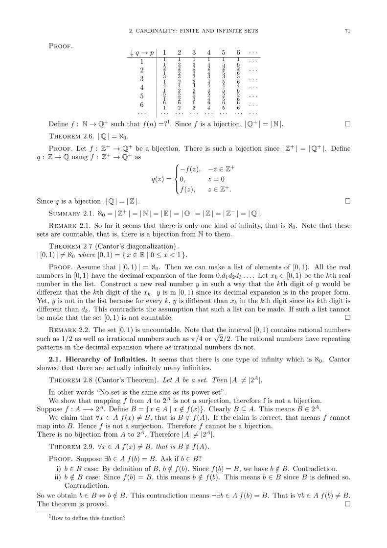
2. CARDINALITY: FINITE AND INFINITE SETS 71

Proof.

# q ! p 1 2 3 4 5 6 · · ·1 1

112

13

14

15

16 · · ·

2 21

22

23

24

25

26 · · ·

3 31

32

33

34

35

36 · · ·

4 41

42

43

44

45

46 · · ·

5 51

52

53

54

55

56 · · ·

6 61

62

63

64

65

66 · · ·

· · · · · · · · · · · · · · · · · · · · · · · ·Define f : N! Q+ such that f(n) =?1. Since f is a bijection, |Q+ | = |N |. ⇤Theorem 2.6. |Q | = @0.

Proof. Let f : Z+ ! Q+ be a bijection. There is such a bijection since |Z+ | = |Q+ |. Defineq : Z! Q using f : Z+ ! Q+ as

q(z) =

8><

>:

�f(z), �z 2 Z+

0, z = 0

f(z), z 2 Z+.

Since q is a bijection, |Q | = |Z |. ⇤Summary 2.1. @0 = |Z+ | = |N | = |E | = |O | = |Z | = |Z� | = |Q |.Remark 2.1. So far it seems that there is only one kind of infinity, that is @0. Note that these

sets are countable, that is, there is a bijection from N to them.

Theorem 2.7 (Cantor’s diagonalization).| [0, 1) | 6= @0 where [0, 1) = {x 2 R | 0 x < 1 }.

Proof. Assume that | [0, 1) | = @0. Then we can make a list of elements of [0, 1). All the realnumbers in [0, 1) have the decimal expansion of the form 0.d1d2d3 . . . . Let x

k

2 [0, 1) be the kth realnumber in the list. Construct a new real number y in such a way that the kth digit of y would bedi↵erent that the kth digit of the x

k

. y is in [0, 1) since its decimal expansion is in the proper form.Yet, y is not in the list because for every k, y is di↵erent than x

k

in the kth digit since its kth digit isdi↵erent than d

k

. This contradicts the assumption that such a list can be made. If such a list cannotbe made that the set [0, 1) is not countable. ⇤

Remark 2.2. The set [0, 1) is uncountable. Note that the interval [0, 1) contains rational numberssuch as 1/2 as well as irrational numbers such as ⇡/4 or

p2/2. The rational numbers have repeating

patterns in the decimal expansion where as irrational numbers do not.

2.1. Hierarchy of Infinities. It seems that there is one type of infinity which is @0. Cantorshowed that there are actually infinitely many infinities.

Theorem 2.8 (Cantor’s Theorem). Let A be a set. Then |A| 6= |2A|.In other words “No set is the same size as its power set”.We show that mapping f from A to 2A is not a surjection, therefore f is not a bijection.

Suppose f : A �! 2A. Define B = {x 2 A | x /2 f(x)}. Clearly B ✓ A. This means B 2 2A.We claim that 8x 2 A f(x) 6= B, that is B /2 f(A). If the claim is correct, that means f cannot

map into B. Hence f is not a surjection. Therefore f cannot be a bijection.There is no bijection from A to 2A. Therefore |A| 6= |2A|.

Theorem 2.9. 8x 2 A f(x) 6= B, that is B /2 f(A).

Proof. Suppose 9b 2 A f(b) = B. Ask if b 2 B?

i) b 2 B case: By definition of B, b /2 f(b). Since f(b) = B, we have b /2 B. Contradiction.ii) b /2 B case: Since f(b) = B, this means b /2 f(b). This means b 2 B since B is defined so.

Contradiction.

So we obtain b 2 B , b /2 B. This contradiction means ¬9b 2 A f(b) = B. That is 8b 2 A f(b) 6= B.The theorem is proved. ⇤

1How to define this function?

72 10. COUNTING

Remark 2.3. Using the Theorem 2.8 we can obtain infinitely many infinities based on N. LetN0 = N. Then |2N| 6= |N|. We can extend this as follows:

DefineN1 = 2N0

N2 = 2N1

. . .. Then

|N1| 6= |N0||N2| 6= |N1|. . .

.

Remark 2.4. The set of real numbers also produces an other chain of infinities as follows: LetR0 = R. Then |2R| 6= |R|. We can extend this as follows:

DefineR1 = 2R0

R2 = 2R1

. . .. Then

|R1| 6= |R0||R2| 6= |R1|. . .

.

Question 2.1. Are the hierarchies of N0, N1, . . . and R0, R1, . . . related or di↵erent?

3. The Number of Ways

Suppose there are n1 ways to go from A to B and n2 ways to go from C to D.

� ))A n1

))5555B

(( � � ))C n2

))5555D

(( � .

3.1. The Product Rule.

Remark 3.1. Let A and B be finite sets where |A | = ↵ and |B | = �.

Theorem 3.1 (The Product Rule).Suppose A� B and C �D are connected in serial. The number of di↵erent ways to go from ⇤ to 4is n1 ⇥ n2.

⇤ ))A n1

))5555B

(( � ))C n2

))5555D

)) 4 .

Theorem 3.2 (The number of elements of cartesian product).Let A be finite set. Then |An | = |A |n.

Proof. By induction on n using the product rule. ⇤Corollary 3.3 (The number of bit strings of length n).

Let Bn be the the set of bit strings of length n where B = { 0, 1 }. Then |Bn | = 2n.

Theorem 3.4 (The number of truth tables).There are 22

ndi↵erent truth tables for propositions in n variables.

Proof. There are 2n rows in a truth table of n variables. For each row, one can assign twochoices, namely F or T. Hence there are 22

ndi↵erent assignments. ⇤

The following theorem will be proved in steps.

Theorem 3.5 (The number of various type of functions).

The number of

functionsinjectionssurjectionsbijectionspartial functions

from A to B is

�↵

�↵

?�!(� + 1)↵

.

3. THE NUMBER OF WAYS 73

Proof. The number of functions from A to B, that is��BA

�� = |B ||A |.Since A is finite, the elements of A can be listed as (a1, a2, . . . , a↵). Use this ordering of elements:

For

a1 2 Aa2 2 A. . .a↵

2 A

, there are

��. . .�

di↵erent choices for

f(a1) 2 Bf(a2) 2 B. . .f(a

↵

) 2 B

.

By product rule, there are �� . . .� = �↵ di↵erent ways. ⇤

Proof. The number of injections from A to B is �↵.If |A | > |B |, then there is no injection from A to B. So consider the case of |A | |B |. Since A isfinite, the elements of A can be listed. Use this ordering of elements:

For

a1 2 Aa2 2 A. . .a↵

2 A

, there are

� � 0� � 1. . .� � (↵� 1)

di↵erent choices for

f(a1) 2 Bf(a2) 2 B. . .f(a

↵

) 2 B

.

By product rule, there are (� � 0)(� � 1) . . . (� � (↵� 1)) = �↵ di↵erent ways. ⇤

Example 3.1. A common approach to counting is to define a bijection to a set whose cardinalityis already known.

We prove that the number of bit strings of length n is |Bn | = 2n by defining a bijection toB{ 1,2,...,n } whose cardinality is 2n. Consider the set B{ 1,2,...,n } of functions from { 1, 2, . . . , n } to B.Define a function

f : B{ 1,2,...,n } ! { 0, 1 }n

g 7! (b1, b2, . . . , bn)

where g 2 B{ 1,2,...,n } and bi

= g(i), i 2 { 1, 2, . . . , n }.f is a bijection (proof?). Therefore

|Bn | =��B{ 1,2,...,n }

�� = |B || { 1,2,...,n } | = 2n.

Remark 3.2. IPv4 is the currently used protocol for the Internet in which every device on theInternet should have a unique ID. IPv4 uses 32-bit IDs which is usually written as four numbersseparated by dots as in the case of 127.0.0.1. Therefore 232 devices can be connected to the Internetat a given time. Although it is a very big number, it is not big enough for the demand of the future.IPv6 is planned to use 128-bit ID’s.

Theorem 3.6 (The number of subsets).Let A be a finite set. Then

�� 2A�� = 2|A | = 2↵.

Proof. Use ↵-tuple (a1, a2, . . . , a↵) of A. Define a function

f : 2A ! B↵

A 7! (b1, b2, . . . , b↵)

where A 2 2A and bi

=

(1, a

i

2 A,

0, ai

/2 A..

f is a bijection (proof?). Therefore�� 2A

�� = |B↵ | = 2↵ = 2|A |. ⇤

Theorem 3.7. Let A1, A2, . . . , An

be finite sets. Then |A1 ⇥A2 ⇥ . . .⇥An

| = |A1 | |A2 | · · · |An

|

3.2. The Sum Rule.

Theorem 3.8 (The Sum Rule).Suppose A�B and C �D is connected in parallel. The number of di↵erent ways to go from ⇤ to 4is n1 + n2.

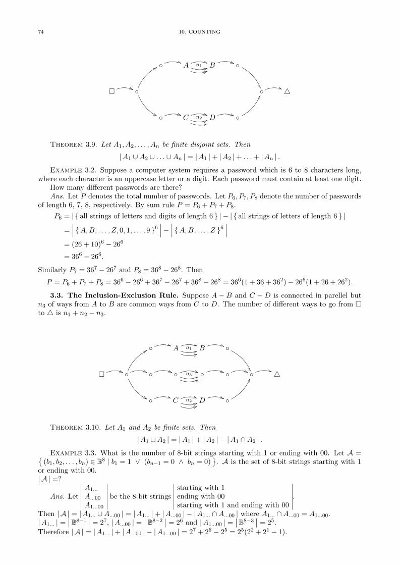
74 10. COUNTING

� ))A n1

))5555B

(( �

��⇤ (( �

88

&&

� ** 4

� ))C n2

))5555D

(( �

HH

Theorem 3.9. Let A1, A2, . . . , An

be finite disjoint sets. Then

|A1 [A2 [ . . . [An

| = |A1 |+ |A2 |+ . . .+ |An

| .

Example 3.2. Suppose a computer system requires a password which is 6 to 8 characters long,where each character is an uppercase letter or a digit. Each password must contain at least one digit.

How many di↵erent passwords are there?Ans. Let P denotes the total number of passwords. Let P6, P7, P8 denote the number of passwords

of length 6, 7, 8, respectively. By sum rule P = P6 + P7 + P8.

P6 = | { all strings of letters and digits of length 6 } |� | { all strings of letters of length 6 } |

=�� {A,B, . . . , Z, 0, 1, . . . , 9 }6

�� {A,B, . . . , Z }6

��

= (26 + 10)6 � 266

= 366 � 266.

Similarly P7 = 367 � 267 and P8 = 368 � 268. Then

P = P6 + P7 + P8 = 366 � 266 + 367 � 267 + 368 � 268 = 366(1 + 36 + 362)� 266(1 + 26 + 262).

3.3. The Inclusion-Exclusion Rule. Suppose A � B and C � D is connected in parellel butn3 of ways from A to B are common ways from C to D. The number of di↵erent ways to go from ⇤to 4 is n1 + n2 � n3.

� ))A n1

))5555B

(( �

��⇤ (( �

88

&&

(( � (( � n3((6666 �

(( � (( � ** 4

� ))C n2

))5555D

(( �

HH

Theorem 3.10. Let A1 and A2 be finite sets. Then

|A1 [A2 | = |A1 |+ |A2 |� |A1 \A2 | .

Example 3.3. What is the number of 8-bit strings starting with 1 or ending with 00. Let A =�(b1, b2, . . . , bn) 2 B8 | b1 = 1 _ (b

n�1 = 0 ^ bn

= 0) . A is the set of 8-bit strings starting with 1

or ending with 00.| A | =?

Ans. LetA1...

A...00

A1...00

be the 8-bit stringsstarting with 1ending with 00starting with 1 and ending with 00

.

Then | A | = |A1... [A...00 | = |A1... |+ |A

...00 |� |A1... \A...00 | where A1... \A

...00 = A1...00.|A1... | =

��B8�1�� = 27, |A

...00 | =��B8�2

�� = 26 and |A1...00 | =��B8�3

�� = 25.Therefore | A | = |A1... |+ |A

...00 |� |A1...00 | = 27 + 26 � 25 = 25(22 + 21 � 1).

5. COUNTING METHODS 75

Table 1. Summary of Counting Methods

ordered unordered

with repetition nr

�n+r�1

r

�

without repetition P(n, r) = n!(n�r)! = nr

�n

r

�= P(n,r)

r! = n!(n�r)!r! =

n

r

r!

Theorem 3.11. Let P be the set of partial functions from A to B. Then | P | = (� + 1)↵.

Proof. Let B = B[{ b0 } where b0 /2 B. Let p 2 P. Define setAp

= { a 2 A | p(a) is not defined }.Then define function p⇤ : A! B such that

p⇤(a) =

(p(a), a 2 A\A

p

,

b0, a 2 Ap

.

Note that p⇤ is a function. Then define function f as

f : P ! BA

p 7! p⇤

f is a bijection (proof ?). Hence | P | =��BA

�� = | B ||A | = (� + 1)↵ ⇤

4. The Pigeonhole Principle

Theorem 4.1 (The Pigeonhole Principle).If k + 1 or more objects are placed into k boxes, then there is at least one box containing 2 or moreobjects.

Theorem 4.2. Among any n+ 1 positive integers not exceeding 2n, there must be an integer thatdivides one of the other integers.

Theorem 4.3 (The Generalized Pigeonhole Principle).If n objects are placed into k boxes, then there is at least one box containing at least dn/k e objects.

Theorem 4.4. Let A and B be finite sets and f : A ! B be a function. If |A | > |B |, then fcannot be an injection.

Proof. Assume that f is an injection. Then f maps each a 2 A into di↵erent b 2 B. Since|A | > |B | by pigeonhole principle, 9a1, a2 2 A [f(a1) = f(a2) = b] for some b 2 B. Hence f cannotbe injective. ⇤

Example 4.1. Let Ai

= (xi

, yi

) i = 1, 2, . . . , 5 be a set of five distinct points with integer coordi-nates in the xy-plane.

Show that the midpoints of the line joining at least one pair of these points have integer coordinates.

Ans.⇣xi+xj

2 , yi+yj

2

⌘is the coordinate of the mid point of A

i

and Aj

. Notice that in order to have

its coordinates integer, xi

+ xj

and yi

+ yj

should be both even. For (xi

, yi

) pair there are four boxes,these are (O,O), (O,E), (E,O), (E,E) where E and O represent even and odd numbers, respectively.Since there are five points, by the pigeonhole principle, two of them should be in the same box. Takethese two points. Their mid point has integer coordinates since x

i

+ xj

and yi

+ yj

are even numbers.

5. Counting Methods: Permutation, Combination and Others

Many counting problems can be put into the following form:There are n objects. Select r of them (r n). Then the result depends on the following questions

as given in Table 1:i. Can an item be reselected? That is, is repetition allowed?ii. Is order of items important?

Definition 5.1. Let A be any finite set. A permutation � of A is a bijection from A to itself.

Remark 5.1. If |A | = n, then it is represented as

� =

✓a1 a2 · · · a

n

ai1 a

i2 · · · ain

◆=�ai1 a

i2 · · · ain

�

where f(aj

) = aij with i, j, i

j

2 { 1, . . . , n }.

76 10. COUNTING

Definition 5.2. The number of distinct subsets with r elements that can be chosen from a setwith n elements is called binomial coe�cient , denoted by

�n

r

�, and is pronounced “n choose r”.

Theorem 5.1. For n, r 2 N, the binomial coe�cients satisfy the following recurrence relation:

i. ✓n

0

◆=

✓n

n

◆= 1

ii. ✓n

r

◆=

✓n� 1

r

◆+

✓n� 1

r � 1

◆for 0 < r < n.

Remark 5.2. Note that Theorem 5.1 leads to the famous Pascal’s triangle.1 2 3 4 5 6 7 8 9 10

1 1 1 1 1 1 1 1 1 1 12 1 2 3 4 5 6 7 8 93 1 3 6 10 15 21 28 364 1 4 10 20 35 56 845 1 5 15 35 70 1266 1 6 21 56 1267 1 7 28 848 1 8 369 1 9

10 1The numbers in the first column are the natural numbers. The numbers in the second and the third

columns are called the triangular and tetrahedral numbers, respectively. The nth triangular numberis simply the sum of the first n integers. The tetrahedral numbers are the sums of the triangularnumbers.

History of binomial coe�cients and Pascal’s triangle goes way back than Pascal. The Pythagoreansconsidered the triangular numbers around 540 BC. The Greek mathematicians investigated tetrahedralnumbers at the beginning of 200 BC. The binomial numbers as coe�cients of (a + b)n appeared inthe works of mathematicians in China around 1100. Hindu mathematicians began to encounter thebinomial coe�cients in combinatorial problems in 1150s. Pascal puts his triangle in 1665.

Theorem 5.2. For n, r 2 N and r n,✓n

r

◆=

n!

(n� r)!r!=

nr

r!.

Theorem 5.3. ✓n

r

◆=

✓n

n� r

◆.

Example 5.1. Let A be a set with n elements. We want to count the number of distinct subsetsof the set A that have exactly r elements.

Example 5.2. Consider A = { a, b, c, d, e }.i. How many di↵erent words of length 3?

Ans. 5⇥ 5⇥ 5 = 53 = 125. Note that each f 2 A{ 1,2,3 } give a di↵erent word.ii. How many di↵erent words of length 3 if no letter is allowed to repeat?

Ans. 5 ⇥ 4 ⇥ 3 = 53 = 60. Note that each f 2 A{ 1,2,3 } where f is an injection gives a di↵erentword.

iii. How many di↵erent words of length 3 if the order of letters is not important?Ans. There are 53 words with order. Each letter combination is counted 3! = 6 times. So53

3! =�53

�= 10

iv. How many di↵erent words of length 3 if letters are allowed to repeat but the order of the lettersis not important?Ans.

6. SUPPLEMENTARY MATERIALS 77

aaa bbb ccc ddd eee 12345673 - - - - 00011112 - 1 - - 0011011- 1 - 1 1 10110102 1 - - - 0010111

Notice that problem is equivalent to selecting 3 balls out of 5 di↵erent boxes. Hence�5+3�1

3

�.

Example 5.3. How many bit strings of length n contains exactly r 1’s?Ans. r positions out of n positions are selected and set to 1. The remaining n � r positions are

set to 0. The order of r positions is not important. So�n

r

�.

Example 5.4. How many ways are there for 8 men and 5 women to stand in a line so that no twowomen stand next to each other, given that all the women are identical, as well as the men?

Ans. There are 9 positions separated by men so that no two women stand next to each other. So�95

�= 126.

men 1 2 3 4 5 6 7 8women 1 2 3 4 5 6 7 8 9

Example 5.5.i. How many solutions does the equation x1 + x2 + x3 = 11 have, where x1, x2, x3 2 N?

Ans. Note that since 1+ 1+1+1+1+1+1+1+1+1+1 = 11 the pattern 11/1111/11111which corresponds to 2+4+5 is a solution. So the number of solutions is

�11+3�12

�.

ii. The same question with constraint x1 � 1, x2 � 2, x3 � 3?Ans. Pick 1 of type 1, 2 of type 2, and 3 of type 3. Then there are additional 5 selections out

of 3 item types. So�5+3�1

5

�.

Example 5.6. How many ways are there to place 10 indistinguishable balls into 8 distinguishablebins? (Consider atoms. Electrons are indistinguishable. The energy levels of an atom are distinguish-able.)

Ans. Rephrase the problem as 10 balls and 7 separators. So�10+8�1

7

�.

Example 5.7. Suppose that S is a set with n elements. How many ordered pairs (A,B) are theresuch that A and B are subsets with A ✓ B?

Ans. {A,BrA,SrB } is a partition of S. So any a 2 S should belong to one of them. Since Sis finite, one can list its elements as (s1, s2, . . . , sn). Let

bi

=

8><

>:

0, si

2 A,

1, si

2 BrA,

2, si

2 SrB.

Then for any (b1, b2, . . . , bn) 2 { 0, 1, 2 }n, define A = { si

| bi

= 0 } and B = { si

| bi

= 0 _ bi

= 1 },hence A ✓ B. Notice that we define a bijection between the set of ternary n-tuples { 0, 1, 2 }n) andour set of (A,B) pairs. So the number is equal to the number of ternary n-tuples, that is 3n.

6. Supplementary Materials

6.1. Some Useful Sequences. A great source of sequences is so called The On-Line Encyclo-pedia of Integer Sequences (OEIS) [Slo09]) available at https://oeis.org/. It is a catalog of more than150000 sequences. It is a great source for combinatorics.

Definition 6.1. The Stirling number , S(n, k) is the number of ways to partition a set of cardinalityn into exactly k nonempty subsets.

Definition 6.2. The nth Bell number , Bn

is the number of partitions of a set with n members,or equivalently, the number of equivalence relations on it. (Sequence A000110 in [Slo09]). It is namedin honor of Eric Temple Bell.

6.2. Approximations for n! and�n

r

�. There is no closed form of n!. Therefore calculating n!

for large n is not easy. It takes too much computation. Some approximations are usually used instead.

https://oeis.org/

https://oeis.org/A000110

78 10. COUNTING

6.2.1. Approximations for n!. Stirling provided an approximation for n! in 1730. Stirling’s ap-proximation is quite good for n � 1 [Rei67, Mac03]. Even as small values as n = 10, the error isless than 1%.

n! = 1⇥ 2⇥ · · ·⇥ n

lnn! = ln 1 + ln 2 + · · ·+ lnn

⇡Z

n

1lnx dx = [x lnx� x|n1 = n lnn� n+ 1

⇡ n lnn� n

n! ⇡ en lnn�n = elnn

ne�n = nne�n.

With the next order of correction, it is:

n! ⇡ nne�n

p2⇡n

lnn! ⇡ n lnn� n+1

2ln(2⇡n).

A better approximation is:

p2⇡n

⇣ne

⌘n

e1/(12n+1) < n! <p2⇡n

⇣ne

⌘n

e1/12n.

6.2.2. Approximations for�n

r

�. Using approximations for n!,

�n

r

�is obtained:

✓n

r

◆=

n!

(n� r)!r!

ln

✓n

r

◆= lnn!� ln(n� r)!� ln r!

⇡ n lnn� n

� ((n� r) ln(n� r)� (n� r))

� (r ln r � r)

= n lnn� (n� r) ln(n� r)� r ln r

= lnnn � ln(n� r)(n�r) ln rr

= lnnn

(n� r)(n�r)rr.

log2

✓n

r

◆= log2

nn

(n� r)(n�r)rr

= log2n(n�r)

(n� r)(n�r)

nr

rr

= log2

✓n

n� r

◆n�r

+ log2⇣nr

⌘r

= (n� r) log2n

n� r+ r log2

n

r

= n

✓(n� r)

nlog2

n

n� r+

r

nlog2

n

r

◆

= n

(n� r)

nlog2

1(n�r)

n

+r

nlog2

1r

n

!

= n

⇣1� r

n

⌘log2

1�1� r

n

� + r

nlog2

1r

n

!

= nH2

⇣ rn

⌘.


where the binary entropy function, H2 (x), is given as

H2 (x) = �x log2 x� (1� x) log2(1� x)

= x log21

x+ (1� x) log2

1

(1� x).

Acknowledgment. These notes are based on various books but especially [Ros07].


P 10.1. Suppose that S is a set with n elements. How many ordered pairs (A,B) are there suchthat A and B are subsets of S with A ✓ B? [Hint: Show that each element of S belongs to A,BrA,or SrB.]

Solution.Let A and B subsets of S with A ✓ B.

8s 2 S [s 2 S] tautology

,8s 2 S [(s 2 B) � (s 2 S �B)] since B ✓ S

) S = B [ (S �B)

and B \ (S �B) = ;,8s 2 S [((s 2 A) � (s 2 B �A)) � (s 2 S �B)] since A ✓ B

) B = A [ (B �A)

and A \ (B �A) = ;Hence, for every s 2 S there are three mutually disjoint alternatives: s belongs to either A or BrA,or SrB. Since the choice for di↵erent elements are independent from each other, the result can befound by the rule of product. The number of ordered pairs is

3 · 3 · · · · · 3| {z }n times

= 3n.

P 10.2. Show that a subset of a countable set is also countable.

Solution.

Let A ✓ B. If A is finite by definition it is countable.Suppose A is infinite. We define a bijection from N to A as follows: Since B is countable there

is a bijection from N to B. Using this bijection we can make a list of elements of B. Use this list,drop all elements that are not in A. This will be a new list which contains only the elements of A.Define a function f : N! A as f(n) 7! a

n

where an

is the nth elements of A in the new list. This isa bijection since for any n 2 N there is a unique a

n

2 A. and vice versa.

P 10.3.

Definition 6.3. A function f : A! A is said to have a fixed point if there exists x 2 A such thatf(x) = x.

Let A = {1, 2, . . . , n} for some n 2 N. How many one-to-one functions f : A ! A have at leastone fixed point?

Solution.

The number of one-to-one functions, which have at least one fixed point, can be computed bysubtracting the number of one-to-one functions, which does not have any fixed points, from thenumber of all one-to-one functions.

The number of all one-to-one functions f : A! A is n!A function which does not have any fixed point is a derangement. The number of derangements

of a set with n element is Dn

where:

Dn

= n!

1� 1

1!+

1

2!� 1

3!+ ....+ (�1)n 1

n!

�.

80 10. COUNTING

Hence the answer is n!�Dn

P 10.4. Show that a subset of a countable set is also countable.

Solution.Let A be a countable set and B be a subset of A.i) If A is finite, then B should be finite too since |B| |A|. Hence B is countable.ii) If A is not finite, then there exists a bijection f : A �! N. If B is finite, it is countable. For infiniteB we can list its elements as follows:

b1 = f�1 (min{ f(b) | b 2 B })b2 = f�1 (min{ f(b) | b 2 B � {b1} })b3 = f�1 (min{ f(b) | b 2 B � {b1, b2} })... = .......

bn

= f�1 (min{ f(b) | b 2 B � {b1, b2, ....., bn�1} })This is equivalent to saying that we are listing B’s elements in the same order as they are listed by f .Hence, B is countable.

CHAPTER 11

Recurrence

1. Motivation

2. Recurrence Equations


P 11.1. Markov chains are powerful models that are often used in Computer Science. In oneapplication of Markov models is the population dynamics where there are two types A and B incompetition with populations n

A

and nB

where the total population nA

+ nB

is constant. So if typeA increases by one, type B should decrease by one. Then, the state i of the system can be representedby the population of A, that is, i = n

A

. Hence there are N + 1 states represented by 0, 1, · · · , N .If the system is in state i, then it moves to state i � 1 and i + 1 with probabilities p

i,i�1 and pi,i+1,

respectively. Then with probability 1� (pi,i�1+ p

i,i+1) it stays in i. The states 0 and N are absorbingstates. When the system gets in one of these, there is no way to leave them, i.e. p0,1 = p

N,N�1 = 0and p0,0 = p

N,N

= 1.Assuming p

i,i�1 = pi,i+1 = a, one obtains the following recurrence equation:

x0 = 0,xi

= axi+1 + (1� 2a)x

i

+ axi�1, 8i 0 < i < N,

xN

= 1.

Solve this recurrence relation.

Solution.The characteristic equation of x

i

= axi+1 + (1� 2a)x

i

+ axi�1 is ar2 � 2ar + a = 0. ar2 � 2ar + a =

a(r2 � 2r + 1) = a(r � 1)2. Since r = 1 is the root with multiplicity 2, the solution would bexi

= (�0 + �1i)ri = �0 + �1i.Use boundry conditions to find the values of �0 and �1.x0 = 0 = �0 + �10 = �0. So �0 = 0.xN

= 1 = �0 + �1N = �1N . So �1 = 1/N .Finally, the solution is x

i

= i/N for i = 0, 1, . . . , N .

P 11.2. Let { an

} and { bn

} be two sequences whose terms are coupled as

an+1 = ↵1an + �1bn

bn+1 = ↵2an + �2bn

where ↵1,↵2,�1,�2 2 R and � = ↵1�2 � ↵2�1 6= 0.Solve a

n

and bn

when a0 = C and b0 = D.

Solution.The degenerated case is when ↵2 = 0 and �1 = 0. In this case the sequences are not coupled and theyare solved separately. That is, a

n

= C↵n

1 and bn

= D�n2 .Consider the non-degenarated case. Assume �1 6= 0. Then

bn

=1

�1(a

n+1 � ↵1an)(1)

bn+1 =

1

�1(a

n+2 � ↵1an+1).(2)

81

82 11. RECURRENCE

Substituting bn

and bn+1 into the second relation, we obtain

0 = bn+1 � ↵2an � �2bn

) 0 =1

�1(a

n+2 � ↵1an+1)� ↵2an ��2�1

(an+1 � ↵1an)

) 0 = (an+2 � ↵1an+1)� �1↵2an � �2(an+1 � ↵1an)

) 0 = an+2 + (�↵1 � �2)an+1 + (�↵2�1 + ↵1�2)an

Let A1 = �↵1 � �2 and A0 = �↵2�1 + ↵1�2. Then an+2 + A1an+1 + A0an = 0. By change of index

an

+ A1an�1 + A0an�2 = 0. Use characteristic root technique to solve an

. Once an

is obtained asan

= f(an�1, an�2), use Eq 1.

Part 6

Graphs

CHAPTER 12

Graphs

1. Introduction

Graph is a very powerful representation used in many disciplines including Computer Science,Management, Physics and of course Mathematics. Interactions, relations of objects are usually repre-sented by a graph.

On the other hand, graphs are used for social entertainment. Remember questions such as “canyou draw this without removing your pencil from the paper” as in Fig. 1.

Example 1.1. Consider www, web pages and links. A web page has links to other web pages.A web page a can have many links to page b but there may be no link from b to a. Your web pageprobably have a link to google.com but you would be very lucky if home page of google.com has a linkto your web page.

A web page can have a link to an item in itself. Long web pages have internal links to headingsin it.

2. Graphs

Definition 2.1 (Multigraph).A Multigraph G = (V,A,' ) consists of a nonempty set V of vertices, a set A of arcs and a function' : A! V ⇥ V

Remark 2.1.• V is nonempty but A could be empty. So, a single vertex with no arcs is the most simple graph.• arcs will be denoted by Greek letters.

• arc �!↵ =��!(u, v) if '(�!↵ ) = (u, v).

• Function ' is in general not an injection. So it is possible that '(�!↵i

) = '(�!↵j

) = (u, v) for �!↵i

6= �!↵j

.

Hence, two vertices can be connected more than once, and therefore��!(u, v) representation of arcs

becomes ambiguous.

Definition 2.2 (Multiplicity).Multiplicity of (u, v) ,

��'�1((u, v))��.

Definition 2.3 (Simple Graph).A simple graph is a multigraph G = (V,A,' ) such that ' is an injection.

Figure 1. Envelope

85

86 12. GRAPHS

Remark 2.2. Multiplicity of any ordered pair (u, v) is at most 1. Therefore (u, v) is su�cient todenote the arc. Hence a simple graph can be represented as G = (V,') where ' is a relation on V .

Remark 2.3. A multigraph G can be represented as G = (V,') where V is the vertex set,' : V ⇥ V ! N is the function expressing the multiplicity of (v1, v2).

Example 2.1.

v1

�!↵1

ss

�!↵3 ''�!

↵5ww

�!↵6

⌥⌥v2

�!↵4

33 v3

�!↵2

gg

v4 �!↵7

++ v5

2

66664

1 2 1 0 00 0 1 0 01 0 0 0 00 0 0 0 10 0 0 0 0

3

77775

path: ��!↵1↵3↵2

simple path: ��!↵4↵2↵1↵5

elementary path: ��!↵6↵4

circuit: ��!↵3↵2

loop: �!↵1

2. GRAPHS 87

Definition 2.4 (Path).

Let G = (V,A,' ) be a multigraph. Given an arc��!(u, v) 2 A, u is called the origin, v is called terminus.

A path P of G is a sequence of arcs �!↵0�!↵1 . . . such that for every pair, �!↵

i

,��!↵i+1, the origin of ��!↵

i+1 isthe terminus of �!↵

i

.

Definition 2.5.

A path which does not traverse the samearcvertex

twice is calleda simple path.an elementary path.

Definition 2.6. Circuit is a finite path such that the origin of the first one coincides with theterminus of the last.

Definition 2.7. Simple circuit is a circuit which is a simple path.

Question 2.1. Define elementary circuit.

Definition 2.8. The number of arcs in a finite path is called the order of the path.

Definition 2.9. A circuit of order 1 is called loop.

2.1. Reachability and Strong-Connectedness.

Definition 2.10. v is said to be reachable from u 2 G = (V,A,' )� ! u = v or there is a path

from u to v.

Definition 2.11. Simple graph G⇤ associated with G is the simple graph obtained by eliminatingall but one of the arcs if the multiplicity is more than 1.

Remark 2.4.i. Connection array M

G

⇤ of G⇤ has only 0s and 1s.ii. [M

G

⇤ ]ij

= 1 means there is an arc from vi

to vj

.

Definition 2.12. Power of a relation on A.

⇢k =

(⇢⇢k�1 k > 1,

⇢ k = 1.

Remark 2.5.• M

⇢

k+1 = M⇢

M⇢

k = (M⇢

)k+1

• ⇢⇢k = ⇢k⇢

Theorem 2.1. Let G = (V, ⇢ ) be a simple graph describing ⇢.There is a path of order n from u to v ! (u, v) 2 ⇢n.

Remark 2.6. Given a simple graph G = (V, ⇢ ), the array (M⇢

)k describes the relation on V :“there is at least one path of order exactly k”. In other words, [(M

⇢

)k]ij

= 1 ! there is at leastone path of order k from v

i

to vj

.

Reachability for G⇤ = (V, ⇢ ) can be obtained by Algorithm 2 where |V | = n.

Algorithm 2: Reachability

/* reachability for G⇤ = (V, ⇢) */

/* where |V | = n */

1 begin2 M(G) M

⇢

+ I3 for k = 2 to n� 1 do4 M(G) M(G) +M

⇢

k

5 end6 end

88 12. GRAPHS

Definition 2.13. G is a multigraph and G⇤ is the associated simple graph.The reachability array M(G) of G is defined as

[M(G)]ij

=

(1, 9k for which [M

⇢

k ]ij

= 1 where 1 k n� 1,

0, otherwise.

Remark 2.7. [M(G)]ij

= 1 ! there is a path from vi

to vj

in G.

Definition 2.14. A multigraph is said to be strongly connected� ! there is a path from v

i

tovj

for all vi

, vj

2 V .

Definition 2.15. G = [V,A,'] is a multigraph, {V1, V2 } dichotomy of V . The set of arcs fromvertices of V1 to vertices of V2 is called the cut-set of G relative to the dichotomy {V1, V2 }.

Example 2.2.

a)Is it strongly connected? No, there is no way to v1.

v11

~~ 2 ''

3

⇠⇠v2 4

//

5

33

6

v48

ss

9

~~ 10wwv3

7

YY

MG

⇤ =

2

664

0 1 0 10 0 0 10 1 0 00 1 1 0

3

775

M(G) = MG

⇤

MG

2 =

2

664

0 1 0 10 0 0 10 1 0 00 1 1 0

3

775 _

2

664

0 1 0 10 0 0 10 1 0 00 1 1 0

3

775

2

664

0 1 0 10 0 0 10 1 0 00 1 1 0

3

775

=

2

664

0 1 0 10 0 0 10 1 0 00 1 1 0

3

775 _

2

664

0 1 1 10 1 1 00 0 0 10 1 0 1

3

775 =

2

664

0 1 1 10 1 1 10 1 0 10 1 1 1

3

775

MG

3 =

2

664

0 1 1 10 1 1 10 1 0 10 1 1 1

3

775 _

2

664

0 1 0 10 0 0 10 1 0 00 1 1 0

3

775

2

664

0 1 1 10 1 1 00 0 0 10 1 0 1

3

775

=

2

664

0 1 1 10 1 1 10 1 0 10 1 1 1

3

775 _

2

664

0 1 1 10 1 0 10 1 1 00 1 1 1

3

775 =

2

664

0 1 1 10 1 1 10 1 1 10 1 1 1

3

775

MG

⇤ = . . . =

2

664

0 1 1 10 1 1 10 1 1 10 1 1 1

3

775 not strongly connected.

b) use V0 = { { v1, v4 } , { v2, v3 } } as an example.Then the cut-set relative to V0 is {↵1,↵8,↵9,↵10 }.

3. UNDIRECTED GRAPHS 89

q00/1

,,1/0,,

q1

0/0tt

1/0

ll

q2

0/0

TT

1/1

YY

Figure 2. State transition diagram

Example 2.3.

Theorem 2.2. G = [V,A,'] is strongly connected ! for every dichotomy {V1, V2 }, the cut-setis non empty.

1

2.2. Application of Multigraphs.• Graphs are used to represent state transition of finite state machines Fig. 2.• Many data structures are represented as graphs Fig. 3, Fig. 4, Fig. 5.• Some other systems are also represented by graphs Fig. 6.• Computer networks• Interconnecting networks• Parallel architectures• Graph algorithms

3. Undirected Graphs

If the relation is symmetric: • (( •hh ⌘ • •Definition 3.1 (Multiple undirected graph).

A multiple undirected graph G = (V,E,' ) consists of a set V of vertices, a set E of edges and afunction ' from E to the set of unordered pairs in V .

Notation. If '(↵) =< u, v > we write (u, v).

Definition 3.2. For (u, v) 2 E, u and v are called terminals.

Definition 3.3. A chain is a sequence of edges (v0, v1)(v1, v2)(v2, v3) · · · (vn�1, vn).A simple chain if no edge is repeated.An elementary chain if no vertices is repeated.A cycle if v0 = v

n

A simple cycle ⌘ simple chain + cycle.

Definition 3.4. G = (V,E,' ) is connected� ! 8v1, v2 2 V [there is a chain between v1 and

v2].

1 @HB check

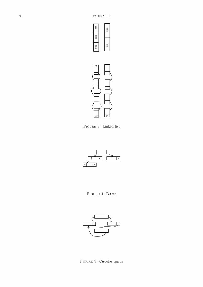
90 12. GRAPHS

Figure 3. Linked list

Figure 4. B-tree

Figure 5. Circular queue

3. UNDIRECTED GRAPHS 91

Figure 6. Flow chart

Definition 3.5. Let G be an undirected graph. The corresponding adjoint multigraph, GA, isobtained by replacing each edge by a pair of opposite arcs.

Definition 3.6 (Subgraph).G0 = (V 0, E0,'0 ) is called a subgraph of G = (V,E,' ) if V 0 ✓ V , E0 ✓ E and E0 consists of all theedges in E joining vertices in V 0. If E0 is a subset of all the edges in E joining vertices in V 0, then G0

is called partial subgraph.

Definition 3.7. A component G0 of G is a connected subgraph such that no vertex in V 0 isconnected to a vertex in V \ V 0 in G.

Theorem 3.1. Let G be an undirected multigraph.G is connected ! GA is strongly connected. ! “something similar to cut-set theorem”. ! G has only one component.

Theorem 3.2. A connected undirected simple graph with |V | = n � 1, must have at least n � 1edges.

Definition 3.8. Let G = (V,E,' ) be connected. A vertex v is called a cut-point if the subgraphobtained by deleting it is not connected.

Theorem 3.3. v is a cut-point ! there exist vertices u and w such that every chain connectingu and w passes through v.

Example 3.1.

a 1

2

3 4

b

5 6

c 7

12

d 8

9 10

e

13

f 11 g

h

i. A simple chain which is not an elementarychain: 4, 9, 11, 10, 5.

ii. A simple cycle: 9, 10, 11 or 1, 6, 13, 12, 3.iii. Is G connected? Yes.iv. How many components does G have? 1.

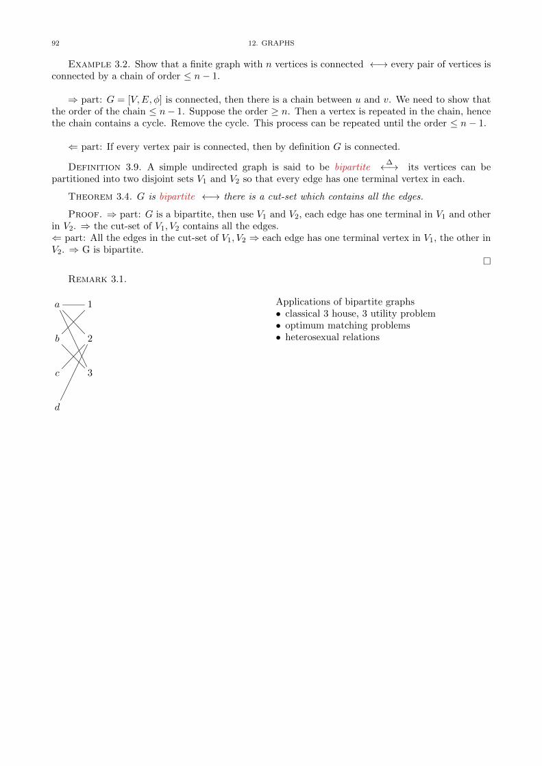
92 12. GRAPHS

Example 3.2. Show that a finite graph with n vertices is connected ! every pair of vertices isconnected by a chain of order n� 1.

) part: G = [V,E,�] is connected, then there is a chain between u and v. We need to show thatthe order of the chain n� 1. Suppose the order � n. Then a vertex is repeated in the chain, hencethe chain contains a cycle. Remove the cycle. This process can be repeated until the order n� 1.

( part: If every vertex pair is connected, then by definition G is connected.

Definition 3.9. A simple undirected graph is said to be bipartite� ! its vertices can be

partitioned into two disjoint sets V1 and V2 so that every edge has one terminal vertex in each.

Theorem 3.4. G is bipartite ! there is a cut-set which contains all the edges.

Proof. ) part: G is a bipartite, then use V1 and V2, each edge has one terminal in V1 and otherin V2. ) the cut-set of V1, V2 contains all the edges.( part: All the edges in the cut-set of V1, V2 ) each edge has one terminal vertex in V1, the other inV2. ) G is bipartite.

⇤Remark 3.1.

a 1

b 2

c 3

d

Applications of bipartite graphs• classical 3 house, 3 utility problem• optimum matching problems• heterosexual relations

5. PLANARITY AND COLORATION 93

4. Path Problems

Definition 4.1. For a multigraph G:indegreeoutdegree

of a vertex v is the number of axesterminateoriginated

on v.

Definition 4.2. For an undirected multigraph G, degree of a vertex v is the number of edgesincident on v.

Definition 4.3. isolated vertex is a vertex of degree 0.

Definition 4.4. AnEulerian chainEulerian cycle

in an undirected multigraph is achaincycle

that uses every

edge once and only once.

Theorem 4.1. An undirected multigraph without isolated vertices has an Eulerian cycle ! itis connected and contains no vertices of odd degree.

Theorem 4.2. G = [V,E,'] without isolated vertices has an Eulerian chain ! it is connectedand contains exactly two vertices of odd degrees.

Definition 4.5. AnHamilton pathHamilton circuit

in a multigraph is apathcircuit

which passes through each

of the vertices exactly once.

Definition 4.6. A multigraph is complete if every point of vertices is joined by at least one arc.

Theorem 4.3. Every complete multigraph contains a Hamiltonian path.

shortest path algorithm pp77. Read 2.4.1, 2.4.2, 2.4.3

Question 4.1. G = [V,A,↵]. d+(v) = indegree(v), d�(v) = outdegree(v).Show

Pv2V d+(v) =

Pv2V d�(v) = |A |.

Theorem 4.4. There is even number of vertices which have odd degrees in an undirected multi-graph.

5. Planarity and Coloration

Application. Consider printed circuit boards (PCB) used in electronic devices. Legs of integratedcircuits (IC) are electrically connected by means of channels of the PCB. While channel run on PCB,they should not cross each other. If they do, short circuits occur. So drawing channels withoutcrossing each other becomes an importing issue. Very same problem occurs in the integrated circuitproduction. In this case electronic components such as resistors, transistors are structures on a siliconwafer. There is channels on silicon to connect them electrically. This is problem can be converted tothe problem of drawing a graph on a plane or planarity of graphs.

Definition 5.1. A finite undirected multigraph is planar if it can be drawn on a plane in such away that no two of its edges intersect except, possibly, at vertices.

Definition 5.2. An undirected multigraphG = (V,E,') is said to be n-colorable� ! 9f, f : V !

{ 1, 2, . . . , n } such that if (u, v) 2 E then f(u) 6= f(v).

Theorem 5.1 (The Four-color Theorem).Every planar graph is 4-colorable.

Definition 5.3. Minimum number n for which an undirected multigraph is n-colorable is calledthe chromatic number of the graph.

Theorem 5.2. If the maximum degree of vertices is n, then the chromatic number is less than orequal to n+ 1.

Theorem 5.3. An undirected multigraph is 2-colorable ! it contains no cycles of odd length.

Theorem 5.4. A tree is 2-colorable.

Haluk BINGOL

pair

94 12. GRAPHS

Definition 5.4. Let G be a connected planar graph. A region of G is a domain of the planesurrounded by edges of the graph such that any two points in it can be joined by a line not crossingany edge. The edges touching a region contain a simple cycle called the contour of the region. Tworegions are said to be adjacent if the contours of the two regions have at least one edge in common.

Theorem 5.5 (Euler Formula).If a connected planar graph has ⌫ vertices, e edges and r regions then ⌫ � e+ r = 2.

Theorem 5.6. If G is a connected simple graph without loops, and has ⌫ vertices, e edges and rregions,then 3

2r e 3⌫ � 6.

K3,3 K5

Theorem 5.7 (Kuratowski).An undirected multigraph is planar ! it contains no partial subgraphs of either K3,3 or K5.

6. Tree

Definition 6.1. A tree is a connected undirected graph with no cycles. A tree of an isolatedvertex is called degenerated tree.

Theorem 6.1. Let G = [V,E,↵] and G is a nondegenerated tree. ! every pair of vertices is connected by one and only one chain ! G is connected but deletion of an edge makes it disconnected ! G has no cycles and if an edge is added, one and only one cycle is formed.

Theorem 6.2. A nondegenerated tree contains at least two vertices of degree 1.

Theorem 6.3. G = [V,E,↵] with |V | = n � 1G is a tree ! G contains no cycle and has n-1 edges ! G is connected and has n-1 edges

Definition 6.2 (Spanning Tree).A spanning tree of a connected undirected graph G = [V,E,↵] is a tree T = [V,E

0,↵] where E

0 ✓ Eand ↵

0is the restriction of ↵ to E

0.

Remark 6.1. There may be many spanning trees for G.

Definition 6.3. Aminimal spanning tree is a spanning tree which has minimum number of edges.2

Algorithm 3: The Minimal Spanning Tree Algorithm

1 begin/* minimal spanning tree algorithm here */

2 end

6.1. Minimal Spanning Tree Algorithm.

2@HB correct this

6. TREE 95

6.2. Rooted Tree.

Definition 6.4. A rooted tree R is a directed graph obtained by specifying as the root a specialvertex v and each chain between v and some u is replaced by a path from v to u. The order of thepath from v to u is called the level of u. For every arc (��!u,w), u and w are a predecessor-successorpair. Any vertex whose outdegree is 0 is called a leaf .

Remark 6.2. Rooted trees are classical representations for hierarchical structures.• organization charts

• procedures in programming languages

• algebra of commutative operations

• scope of variables in procedural programming languages

Definition 6.5. An oriented rooted tree is a rooted tree such that the set of arcs issuing from anyvertex is an ordered set.

96 12. GRAPHS

Representation

Example 6.1. Hu↵mann coding is a cod-ing technique which is optimum in mean codinglength.

Acknowledgment. These notes are based on various books but especially [PY73, Ros07,TZ82, Gal89].


P 12.1. Let G = [V,E] be a simple, undirected and connected graph which does not contain anyself-loops. Prove that G is a bipartite graph if and only if G does not contain any cycle of odd length.

Solution.Let G = [V,E] be a loop-free simple, undirected, connected and bipartite graph with V = V1 [ V2.

Let C = {(v1, v2), (v2, v3), (v3, v4), . . . , (vn, v1), } be a cycle in G. Let v1 2 V1. (The proof forv1 2 V2 is similar.) Since G is a bipartite graph v

i

and vi+1 must belong to di↵erent sets V1 and V2.

Hence, the sequence v1 � v2, . . . , vn � v1 is an alternating sequence between the edges of V1 and V2.For this sequence to start and end with the same vertex there must be odd number of vertices in thissequence. Hence, the number of edges on C must be even.

(( Part) Let G = [V,E] be a loop-free simple, undirected and connected graph with no cycles ofodd length. Let x 2 V , andV1 = {v 2 V | the length of a shortest path between x and v is odd} andV2 = {w 2 V | the length of a shortest path between x and w is even}.

Note thati) x 2 V2

ii) V1 \ V2 = ;iii) V1 [ V2 = V .

Claim: each edge {a, b} 2 E has one vertex in V1 and the other vertex in V2.


To prove this claim suppose that there exists an edge e = {a, b} 2 E with a 6= b and a, b 2 V1.(The proof for a, b 2 V2 is similar) Let E

a

= {{a, v1}, {v1, v2}, . . . , {vm�1, x}} be the m edges in ashortest path from a to x and let E

b

= {{b, v10}, {v10, v20}, . . . , {vn�10, x}} be the n edges in a shortest

path from b to x. m and n are both odd since a, b 2 V1.If {v1, v2, . . . , vm�1}\ {v10, v20, . . . , vm�1

0} = ;, then the set of edges C1 = {{a, b}}[Ea

[Eb

is a cycleof odd length in G. Otherwise, let w( 6= x) be the first vertex where the paths come together and let

C2 = {{a, b}} [ {{a, v1}, {v1, v2}, . . . , {vi, w}} [ {{b, v10}, {v10, v20}, . . . , {vj 0, w}}for some 1 i m� 1 and 1 j n� 1. Then either C2 or C1 � C2 is a cycle of odd-length in G.

P 12.2. Suppose d1, d2, . . . , dn 2 Z+ withP

n

i=1 di = 2n� 2. Show that there is a tree that has nvertices with degree sequence d1, d2, . . . , dn.

Solution.Note that 8i [d

i

> 0]. Use induction on the number of vertices n.Case n = 1. Since 2n � 2 = 0, the degree sequence is d1 = 0 only. A degenerated tree with one

vertex satisfies the proposition. Note that d1 = 0 does not actually satisfy the rule that di

> 0. Sothe question should have one more condition such as n > 1. Hence induction should start from n = 2.

Induction Base. n = 2. Since 2n� 2 = 2, the degree sequence can only be d1 = 1, d2 = 1. A treewith 2 vertices connected by an edge satisfies it.

Induction. Assume that it is true for n � 2. Then show that is must be true for n+ 1.Consider a degree sequence d1, d2, . . . , , dn, dn+1. If we can show that there exist vertices v

k

of degree dk

= 1 and v`

of degree d`

> 1, then we can construct such tree as follows: Reindexd1, d2, . . . , dn�1, dn, dn+1 so that we have dn > 1 and d

n+1 = 1. Hence, dn

�1 > 0. By induction hypote-sis, there exists a corresponding tree T with n vertices for the degree sequence d1, d2, . . . , dn�1, dn� 1.Obtain a new tree T 0 by add vertex v

n+1 to T by connecting vn+1 to v

n

. The degree sequence of T 0

becomes d1, d2, . . . , , dn � 1 + 1, dn+1 = 1.

Existence of dk

= 1. Suppose 8i 2 { 1, 2, . . . , n } [di

> 1]. Then di

� 2, soP

n

i=1 di �P

n

i=1 2 =2n > 2n� 2. Since

Pn

i=1 di = 2n� 2, there must be at lease one vertex with dk

< 2, that is dk

= 1.Existence of d

`

> 1. Suppose 8i 2 { 1, 2, . . . , n } [di

= 1]. ThenP

n

i=1 di =P

n

i=1 1 = n < 2n � 2.Since

Pn

i=1 di = 2n� 2, There must be at lease one vertex with dk

> 1.

Bibliography

[Apo] Tom M. Apostol. Introduction to Analytic Number Theory. Springer-Verlag.[Gal89] Steven Galovich. Introduction to Mathematical Structures. Harcourt Brace Jovanovich, Inc., 1989.[GKP98] Ronald L. Graham, Donald E. Knuth, and Oren Patashnik. Concrete Mathematics: A Foundation for Computer

Science. Addison-Wesley, 1998.[Hol60] Paul Holmos. Naive Set Theory. Van Nastrand, 1960.[LP98] Rudolf Lidl and Gunter Pilz. Applied Abstract Algebra. Springer, 1998.[Mac03] David MacKay. Information Theory,Inference, and Learning. Cambridge University Press, 2003.[Men08] Eliott Mendelson. Number Systems and the Foundation of Analysis. Dover, 2008.[Nes09] Ali Nesin. Mathematige Giris: III. Sayma. Nesin Yayincilik, 2009.[PY73] Franco P. Preparata and Raymond T. Yeh. Introduction to Discrete Structures. Addison-Wesley, 1973.[Rei67] Frederick Reif. Berkeley Physics: Statistical Physics. McGraw-Hill, 1967.[Ros07] Kenneth H. Rosen. Discrete Mathematics and its Applications. McGraw-Hill, 2007.[Slo09] N. J. A. Sloane. The On-Line Encyclopedia of Integer Sequences (OEIS), 2009.[Str94] Steven H. Strogatz. Nonlinear Dynamics and Chaos. Perseus Books Publishing, 1994.[TZ82] Gaisi Takeuti and Wilson M. Zaring. Introduction to Axiomatic Set Theory. Springer-Verlag, 1982.[Wik09] Wikipedia. Mersenne Prime, 2009.

99

BIBLIOGRAPHY 101

.

The Notation Index

(a1, a2), 16(a1, a2, . . . , an), 16=

(a1, a2, . . . , an) = (b1, b2, . . . , bn), 16sets, 15

A ⇢ B, 15A ✓ B, 15A⇥B, 16G = (V,A,' ), 85;, 15C 6=0, 5C, 5N, 5Q+, 5Q�, 5Q�0, 5Q0, 5Q 6=0, 5Q, 5R+, 5R�, 5R�0, 5R0, 5R 6=0, 5R, 5Z+, 5Z�, 5Z�0, 5Z0, 5Z 6=0, 5Z, 5|A |, 152A, 16a < b, 31a↵ b, 18a 2 A, 15a /2 A, 15{ a1, a2, . . . }, 15{ a | P (a) }, 15

103

The Concepts Index

binary relation, 18

cardinality, 15cartesian product, 16

dyadic, 11

empty, 16empty set, 15equal

ordered pairs, 16set, 15

finite set, 15function

partial, 20

infinite set, 15

monadic, 11Multigraph, 85

operatordyadic, 11monadic, 11

ordered n�tuple, 16ordered pairs, 16

power set, 16proper subset, 15

relationboolean matrix multiplication, 19complement, 20composition, 19inverse, 20transpose, 20

seta 2 A, 15a /2 A, 15binary relation, 18cardinality, 15cartesian product, 16disjoint, 17element, 15empty set, 15equal, 15finite set, 15infinite set, 15membership, 15ordered n�tuple, 16ordered pairs, 16power set, 16proper subset, 15representation, 15set, 15set operations

complement, 17

di↵erence, 17intersection, 16symmetric di↵erence, 17union, 16

subset, 15subset, 15

truth table, 11

105

Discrete Mathematics Haluk Bingol - CmpE

Documents

Transcript of Discrete Mathematics Haluk Bingol - CmpE