Discrete Isoperimetric Inequalities onGraphs

Senior Seminar

By

Sanjay Shrestha

Department of Mathematics

Saint Marys College of California

Moraga, California

Mentor:Dr. Ellen Veomett

Supervisor:Dr. Kathryn Porter

May 21, 2017

1 Introduction

The topic of this senior thesis project is that of “Discrete Isoperimetric Inequlities on

Graphs”. The word “isoperimetric” refers to sets having the same boundary or same perime-

ter. Isoperimetric problems ask for sets whose volume is smallest with the given perimeter.

The Isoperimetric inequality in the Eucleadean plane refers to among all sets of same perime-

ter which one has the largest area. Zenodorus (200BC - 140 BC), an ancient Greek mathe-

matician proved that, “The circle encloses a greater area than any regular polygon of equal

perimeter”[1]. He also theorized that the sphere has the greatest volume of any solid with the

same surface area. While we will not be talking about spheres and circles in this paper, the

isoperimetric problem on the Euclidean plane helps us to better understand the topic. This

paper is about discrete isoperimetric inequalities on graphs, and in particular on boolean

cubes. We will be discussing both edge isoperimetric problems and vertex isoperimetric

problems. But first, we must define a graph and a boolean cube.

Definition 1. A graph (G) consists of a set of vertices V, and set of edges E ⊂ V × V ,

which can be written as G = (V,E). (Our graphs in this paper do not have weighted vertices

or edges or directed edges.)

Example 1. We can visualize the graph in figure 1 with circular dots as vertices and the line

between them as edges. Define the graph, V = {A,B,C,D} and E = {(A,B), (B,C), (C,D), (D,A)}

where the order of the vertices to each edge does not matter.

Figure 1: Example of a graph

Definition 2. A Boolean cube is a graph G = (V,E) where V = {0, 1}d and {x, y} ∈ E

ifn∑

i=1

|xi − yi| = 1

where x = (x1, x2, ...xn) and y = (y1, y2, ....yn). A Boolean cube is also called a hamming

ball, d-cube or a hypercube. We use the notation Qd to refer it.

Figure 2: Boolean cubes of Q1, Q2 and Q3 respectively

So, we know what a graph is and what a Boolean cube is. Let us finally define the main

topics of this paper: the edge isoperimetric problem and the vertex isoperimetric problem.

Definition 3. For any graph G, and S ⊆ V we define

Θ(S) = {e ∈ E : e = {v, w}, v ∈ S & w 6∈ S}

and we call Θ(S) the edge-boundary of S.

Example 2. In the figure 1, if we consider S = {A,B}, the edge boundary will be Θ(S) =

{AD,BC}.

Definition 4. Given a graph G, if we fix the size of S, |S| = k, the edge isoperimetric

problem is to minimize the size of the edge-boundary over all S ⊆ V with |S| = k. We will

refer to the edge isoperimetric problem with EIP.

Example 3. Consider figure 1. As we said in example 3, Θ{A,B} = {AD,BC}. If we set

|S| = 2 then we can visually convince ourselves that |Θ(S)| = 2 is the smallest boundary

possible. If we choose non incident vertices we get a larger boundary. For example, if we

choose S = {A,C} then Θ(A,C) = {AB,AD,BC,BA} so that |Θ(S)| = 4. The solution of

EIP gives the smallest value of |Θ(S)| among all sets S of size k.

Now we will introduce n-cycle graph to find the solution of the EIP.

2 EIP in n-cycle graph (Zn)

Definition 5. We define a graph Zn = (V,E) where V = {0, 1, 2, 3, .......n − 1} and E =

{(x, y) ∈ V : x− y ≡ 1(mod n)}.

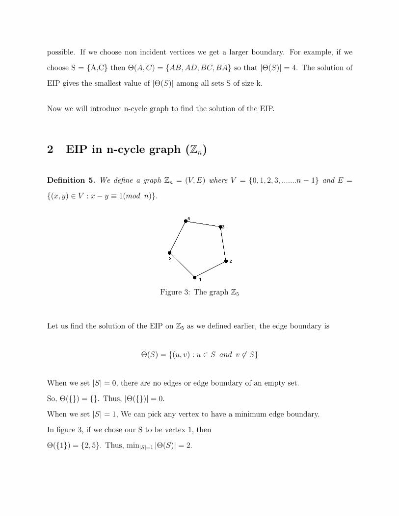
Figure 3: The graph Z5

Let us find the solution of the EIP on Z5 as we defined earlier, the edge boundary is

Θ(S) = {(u, v) : u ∈ S and v 6∈ S}

When we set |S| = 0, there are no edges or edge boundary of an empty set.

So, Θ({}) = {}. Thus, |Θ({})| = 0.

When we set |S| = 1, We can pick any vertex to have a minimum edge boundary.

In figure 3, if we chose our S to be vertex 1, then

Θ({1}) = {2, 5}. Thus, min|S|=1 |Θ(S)| = 2.

Similarly, if we set |S| = 2, We can choose any two vertices that are adjacent to each other.

In the above figure if we chose 1 and 2 to be our vertices then

Θ({1, 2}) = {5, 3}. Thus, |min|S|=2 |Θ(S)| = 2.

In the same manner,

for |S| = 3, we will get min|S|=3 |Θ(S)| = 2,

for |S| = 4, we will get min|S|=4 |Θ(S)| = 2,

for |S| = 5, we will get min|S|=5 |Θ(S)| = 0.

Table 1: Summary of minimum boundary to Zn

k 0 1 2 3 4 5 6 . . n - 1 n|min|S|=kΘ(S) 0 2 2 2 2 2 2 2 2 2 0

From the solution to the EIP of Z5, we can clearly see that for all G and for all S ⊆ V ,

Θ(V −S) = Θ(S) (The proof to this is given below). And min|S|=k |Θ(S)| = min|S|=n−k |Θ(S)|

for k > 1/2|V |.

Theorem 1. For any graph G with G = (V,E) and S ⊆ V , Θ(V − S) = Θ(S).

Proof. Let S ⊆ V By the definition of edge boundary, we have

Θ(S) = {e ∈ E : e = {v, w}, v ∈ S and w 6∈ S}

and

Θ(V − S) = {e ∈ E : e = {v, w}, v ∈ (V − S) & w 6∈ (V − S)}

and we can rewrite,

Θ(V − S) = {e ∈ E : e = {v, w}, v 6∈ S & w ∈ S}

(Since V − S means all the set of vertices that are not in S)

Thus, Θ(V − S) = Θ(S).

Definition 6. The degree of a vertex is the number of edges incident to that vertex.

Example 4. In figure 3, each vertex is incident with two edges. Thus, the degree of each

vertex is 2.

Definition 7. A graph is called regular if every vertex has the same degree.

Example 5. In all of our figures above, each vertex has the same degree, so all of our graphs

above are regular graphs. In the figure below, we can notice certain vertices have degree 4

and some have degree 3, so the graph is not regular. While figure 3 is a regular graph with

each vertices have a degree 2.

Figure 4: Example of a non-regular graph

Definition 8. Let E(S) = {e ∈ E : e = {v, w}, v ∈ S & w ∈ S} then E(S) is called the

induced edges of S.

Example 6. In figure 3, For S{1, 2}, E(S) = E({1, 2}) = {12}.

Lemma 1. If G = (V,E, δ) is a regular graph of degree δ and S ⊆ V , then for all S ⊆ V ,

|Θ(S)|+ 2|E(S)| = δ|S|.

Proof. Assume G = (V,E, δ) is a regular graph of degree δ and S ⊆ V .

Let Θ(S) be the edge boundary and E(S) be the induced edges within S.

On the right hand side of our given equation, we have,

δ|S| where δ is the degree of the graph and |S| is number of vertices in our set S.

δ|S| counts the total number of edges that are connected to S.

While on the left hand side, |Θ(S)| counts the total number of edges that connected with

S but not within S and E(S) counts the edges that are connected from one vertex of S to

another. So, this means you need to count each edge twice inorder to count all degrees of

all vertices of S. Thus, Θ|S|+ 2E(S) is also counting the total number of edges from S.

Therefore, |Θ(S)|+ 2|E(S)| = δ|S|.

Definition 9. The induced edge problem on a graph is to maximize |E(S)| over all

S ⊆ V with |S| = k.

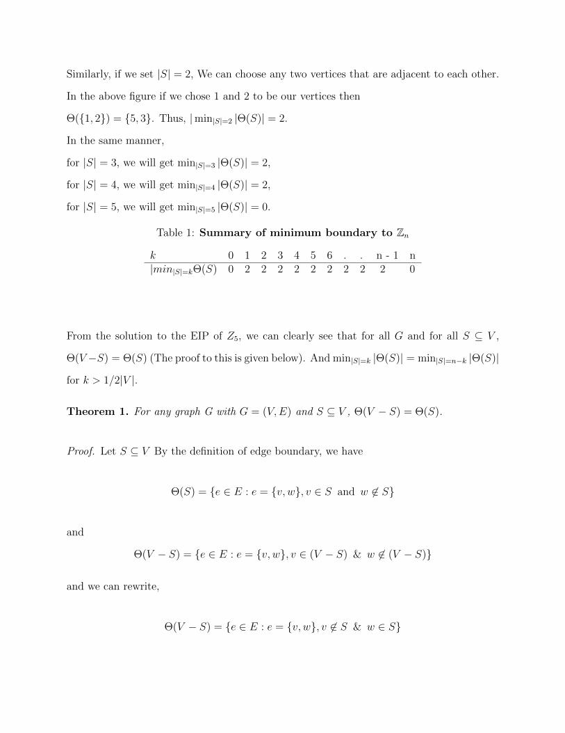
Example 7. In the figure below, if S = {00, 11} then, E(S) = 0 and the size of the edge-

boundary is 4. But for k = 2 and if S = {00, 01}, then we have our maximized |E(S)|. Then

our new size of the edge-boundary is 2 and E(S) = 1.

Corollary 1. If G is a regular graph, then S ⊆ V is a solution of the induced edge problem

iff it is a solution of the EIP. Also for all k min|S|=k |Θ(S)| = δk − 2 max|S|=k |E(S)|.

Proof. Suppose S∗ ⊆ V such that Θ(S∗) is a small as possible and |S∗| = k. From Lemma

1, we know,

|Θ(S∗)| = δk − 2|E(S∗)|.

Now suppose S1 ⊆ V|S1|=k with |E(S1)| > |E(S∗)|

Again from Lemma 1.1, we have

|Θ(S1)| = δk − 2|E(S1)|

< δk − 2|E(S∗)|

= |Θ(S∗)| From Lemma1)

So,|Θ(S1)| < |Θ(S∗)|. This is contradiction. Thus, min|S|=k |Θ(S)| = δk − 2 max|S|=k |E(S)|

and S is solution of the induced edge problem if and only if it is a solution of the EIP.

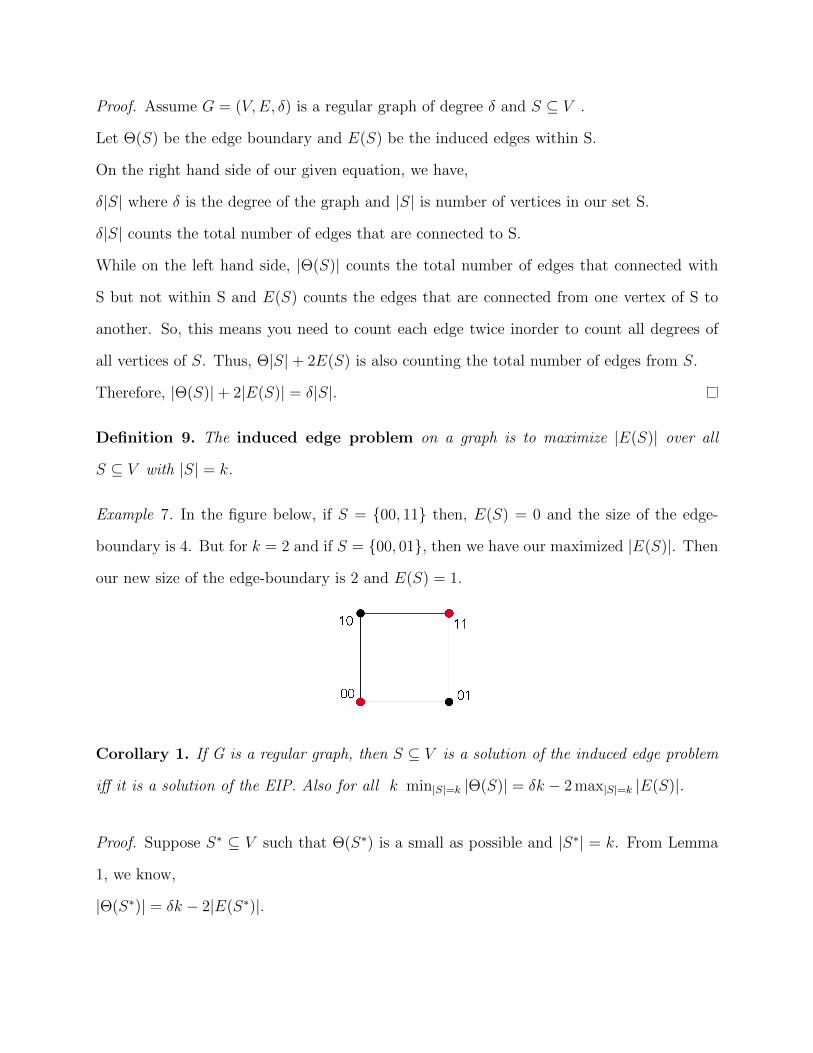
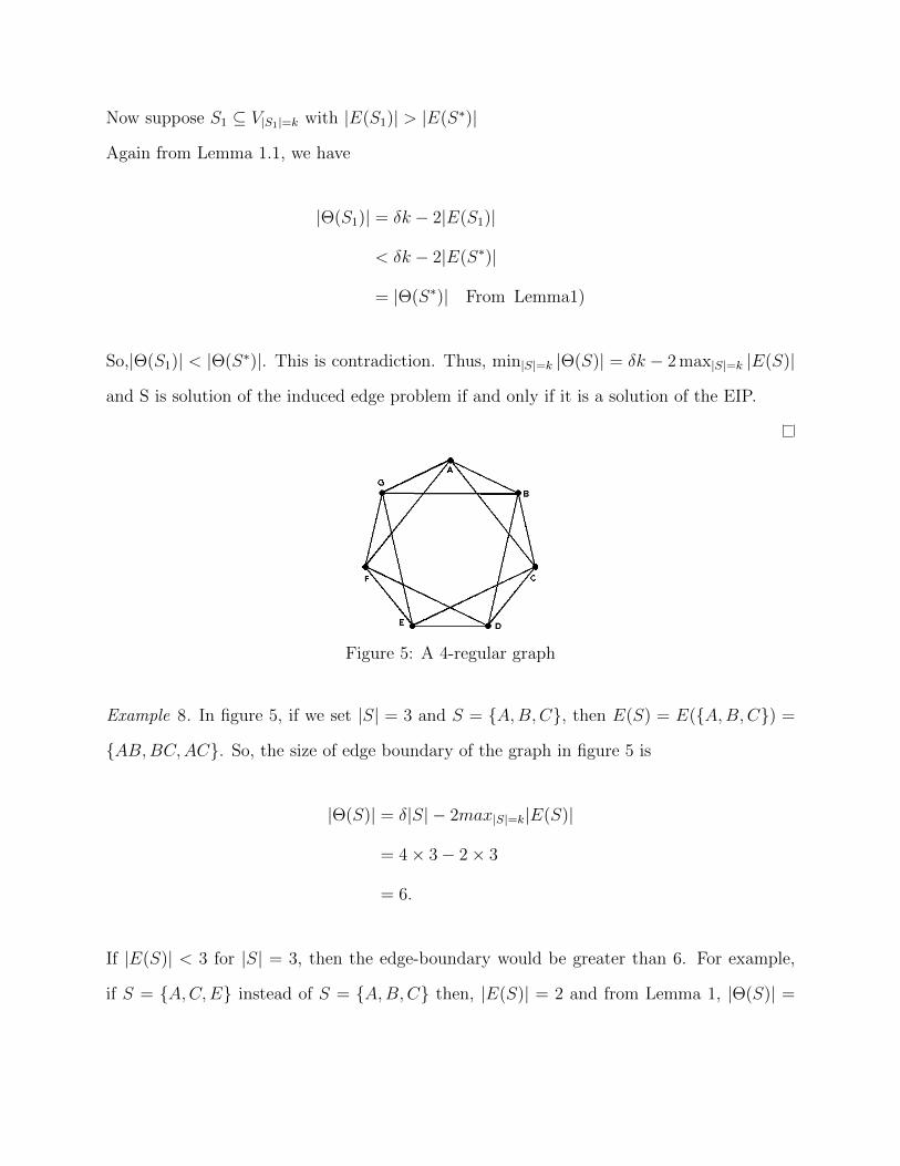
Figure 5: A 4-regular graph

Example 8. In figure 5, if we set |S| = 3 and S = {A,B,C}, then E(S) = E({A,B,C}) =

{AB,BC,AC}. So, the size of edge boundary of the graph in figure 5 is

|Θ(S)| = δ|S| − 2max|S|=k|E(S)|

= 4× 3− 2× 3

= 6.

If |E(S)| < 3 for |S| = 3, then the edge-boundary would be greater than 6. For example,

if S = {A,C,E} instead of S = {A,B,C} then, |E(S)| = 2 and from Lemma 1, |Θ(S)| =

4× 3− 2× 2 = 8. This also shows that whenever we pick our vertices in S, we should pick

vertices in S that are incident to each other which maximizes our incident edge problem.

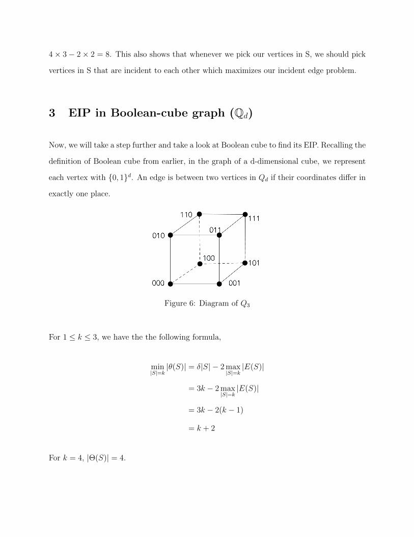
3 EIP in Boolean-cube graph (Qd)

Now, we will take a step further and take a look at Boolean cube to find its EIP. Recalling the

definition of Boolean cube from earlier, in the graph of a d-dimensional cube, we represent

each vertex with {0, 1}d. An edge is between two vertices in Qd if their coordinates differ in

exactly one place.

Figure 6: Diagram of Q3

For 1 ≤ k ≤ 3, we have the the following formula,

min|S|=k|θ(S)| = δ|S| − 2 max

|S|=k|E(S)|

= 3k − 2 max|S|=k|E(S)|

= 3k − 2(k − 1)

= k + 2

For k = 4, |Θ(S)| = 4.

For k ≥ 4,

min|S|=k|Θ(S)| = min

|S|=8−k|Θ(S)|

By now, we can visually calculate EIP for Q3 and the solution is given in the below table.

Table 2: Summary of solution to Q3

k 0 1 2 3 4 5 6 7 8|min|S|=kΘ(S) 0 3 4 5 4 5 4 3 0

Definition 10. Lexicographic ordering is the ordering of vertices in the binary numbering

system with 0 and 1.

We use W.H.Kautz’s lexicographic numbering formula to find the initial segment, which is

given by

lex(x) = 1 +d∑

i=1

x(d−i+1)2i−1

where,

d is the dimension of the Boolean cube and

i is the length of the the coordinates.

Example 9. Some examples of lexicographic ordering is given in table 3.

Definition 11. Suppose X is a finite ordered set. An initial segment of size k is the first

k elements in X, according to the given order.

The solution to edge isoperimetric problem on a hypercube is an initial segment of the

lexicographic numbering. If we have a graph G, and lexicographically order the vertices of

Table 3: Lexicographic Ordering

Q1 Q2 Q3 Q4 Numbering0 00 000 0000 11 01 001 0001 2

10 010 0010 311 011 0011 4

100 0100 5101 0101 6110 0110 7111 0111 8

1000 91001 101010 111011 121100 131101 141110 151111 16

the graph, then we need to find the initial segment and all the vertices up to the initial

segment will have the minimum edge boundary of that graph.

Figure 7: A lexicographic ordering of Q4

So to find a solution of an EIP using the above lexicographic numbering, let us look at the

following example.

Example 10. For Q3 which is figure 6, if the lexicographic numbering for 101 which comes

out to be |S| = 5 is calculated as

lex(x) = 1 +d∑

i=1

xi2i−1

= 1 + x1 × 20 + x2 × 21 + x3 × 22

= 1 + 1× 1 + 0× 2 + 1× 4

= 6

So, the first six number of the lexicographic numbers are the sets of size 6 with the minimum

boundary. They are {000, 001, 010, 011, 100, 101}.

We will not be proving how the initial segment of the lexicographic ordering is the solution

to edge isoperimetric problem but we will prove the one for Vertex Isoperimetric Problem.

4 Vertex Isoperimetric Problem

Definition 12. For any graph G = (V,E, δ), and S ⊆ V the vertex boundary is

∂(S) = {w ∈ V − S : ∃e ∈ E, e = {v, w} and v ∈ S}

Example 11. In the figure 1, if we set S = {A,B} where S is the set of vertices, the vertex

boundary of S will be Φ(S) = {D,C}.

Definition 13. Given a graph G, if we fix the size of S and an integer k, the vertex

isoperimetric problem is to minimize the size of the vertex-boundary over all vertex sets

S ⊆ V with |S| = k. We will refer to the vertex isoperimetric problem as VIP.

We can also represent the Vertex Isoperimetric Problem as

Φ(A) = {v ∈ V : either v ∈ A or (v, a) ∈ E for some a ∈ A}

Both definition 12 and the above definition are the same, so we will be using the later one.

Definition 12 counts all the vertices that are neighbors of our set S but not the vertices in S

while the above definition counts both.

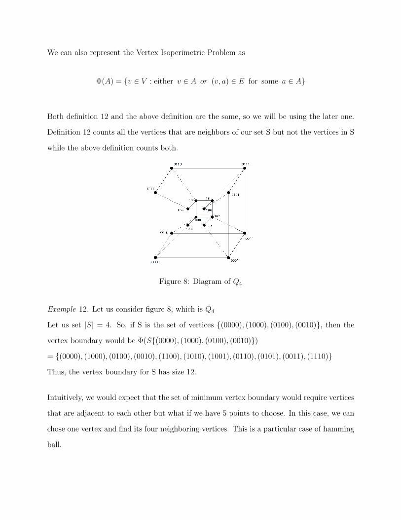
Figure 8: Diagram of Q4

Example 12. Let us consider figure 8, which is Q4

Let us set |S| = 4. So, if S is the set of vertices {(0000), (1000), (0100), (0010)}, then the

vertex boundary would be Φ(S{(0000), (1000), (0100), (0010)})

= {(0000), (1000), (0100), (0010), (1100), (1010), (1001), (0110), (0101), (0011), (1110)}

Thus, the vertex boundary for S has size 12.

Intuitively, we would expect that the set of minimum vertex boundary would require vertices

that are adjacent to each other but what if we have 5 points to choose. In this case, we can

chose one vertex and find its four neighboring vertices. This is a particular case of hamming

ball.

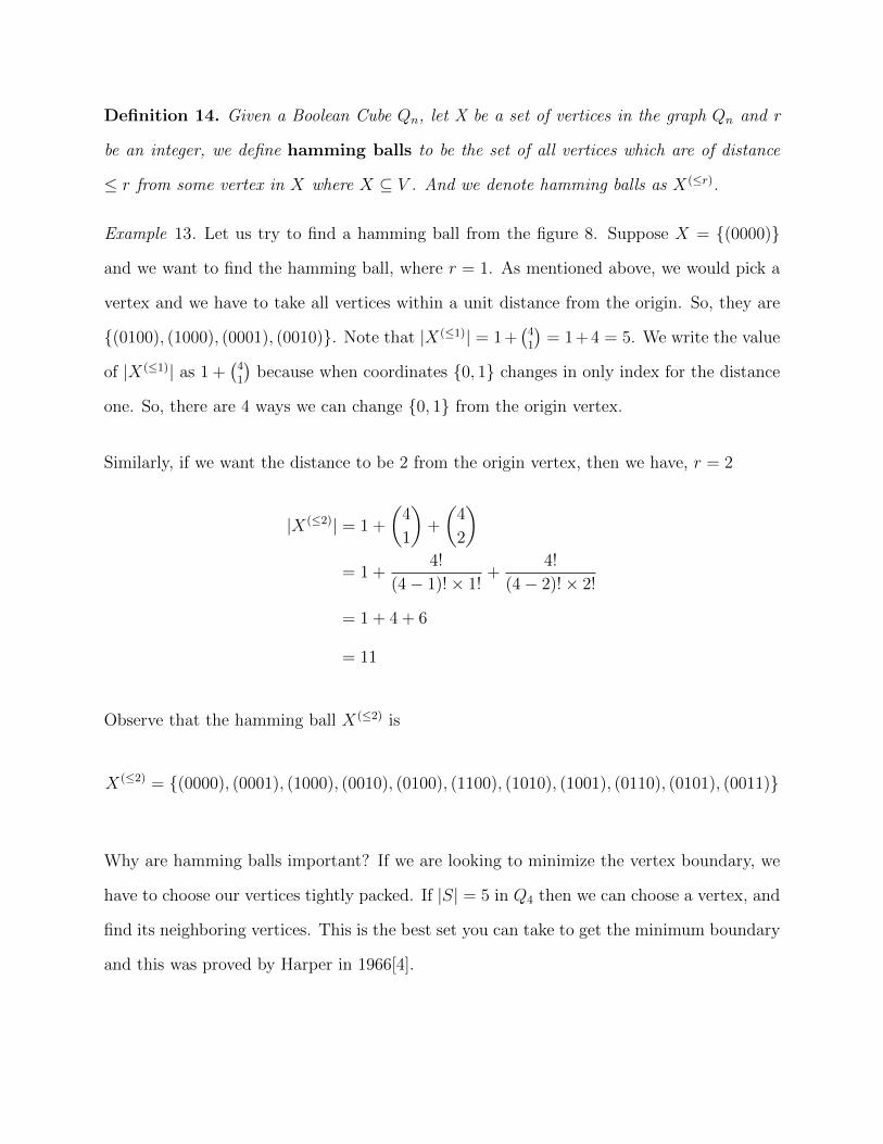
Definition 14. Given a Boolean Cube Qn, let X be a set of vertices in the graph Qn and r

be an integer, we define hamming balls to be the set of all vertices which are of distance

≤ r from some vertex in X where X ⊆ V . And we denote hamming balls as X(≤r).

Example 13. Let us try to find a hamming ball from the figure 8. Suppose X = {(0000)}

and we want to find the hamming ball, where r = 1. As mentioned above, we would pick a

vertex and we have to take all vertices within a unit distance from the origin. So, they are

{(0100), (1000), (0001), (0010)}. Note that |X(≤1)| = 1+(41

)= 1+4 = 5. We write the value

of |X(≤1)| as 1 +(41

)because when coordinates {0, 1} changes in only index for the distance

one. So, there are 4 ways we can change {0, 1} from the origin vertex.

Similarly, if we want the distance to be 2 from the origin vertex, then we have, r = 2

|X(≤2)| = 1 +

(4

1

)+

(4

2

)= 1 +

4!

(4− 1)!× 1!+

4!

(4− 2)!× 2!

= 1 + 4 + 6

= 11

Observe that the hamming ball X(≤2) is

X(≤2) = {(0000), (0001), (1000), (0010), (0100), (1100), (1010), (1001), (0110), (0101), (0011)}

Why are hamming balls important? If we are looking to minimize the vertex boundary, we

have to choose our vertices tightly packed. If |S| = 5 in Q4 then we can choose a vertex, and

find its neighboring vertices. This is the best set you can take to get the minimum boundary

and this was proved by Harper in 1966[4].

Figure 9: Hamming ball of different sizes starting with red vertex

But what if our vertex lies between two successive hamming balls? For example for Q4,

our hamming balls are of size 1,5,11 and 15. We are not able to use Harper’s Theorem on

hamming balls to find the minimum boundary if our size of the set is between 1,5 and 11.

So, we must introduce simplicial ordering and Harper’s theorem to solve this problem. Let

us begin by defining simplicial ordering.

Definition 15. Let x, y ∈ {0, 1}d where x = (x1, x2, ...., , , xn) and y = (y1, y2, ......., yn). If

d = 1 then {0, 1}1 = {(0), (1)} and we define (0) < (1) if d > 1 then x < y if x has less

number of 1s than y, or if they have an equal number of 1s, we look at the first index i where

xi 6= yi and define x < y if yi = 1 and y < x if xi = 1

Example 14. The following table shows the simplicial ordering for different dimension of Q.

If we notice, the numbers start increasing from left to right with gradually filling 1 each time

all the way to left and then adding more ones.

In our proof below, we will define a set S which is a subset of Qn and prove that the boundary

of the initial segment of size |S| is no larger than the boundary of S. The initial segment we

defined for the lexicographic ordering is the same for simiplicial ordering as well.

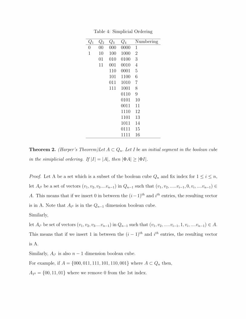
Table 4: Simplicial Ordering

Q1 Q2 Q3 Q4 Numbering0 00 000 0000 11 10 100 1000 2

01 010 0100 311 001 0010 4

110 0001 5101 1100 6011 1010 7111 1001 8

0110 90101 100011 111110 121101 131011 140111 151111 16

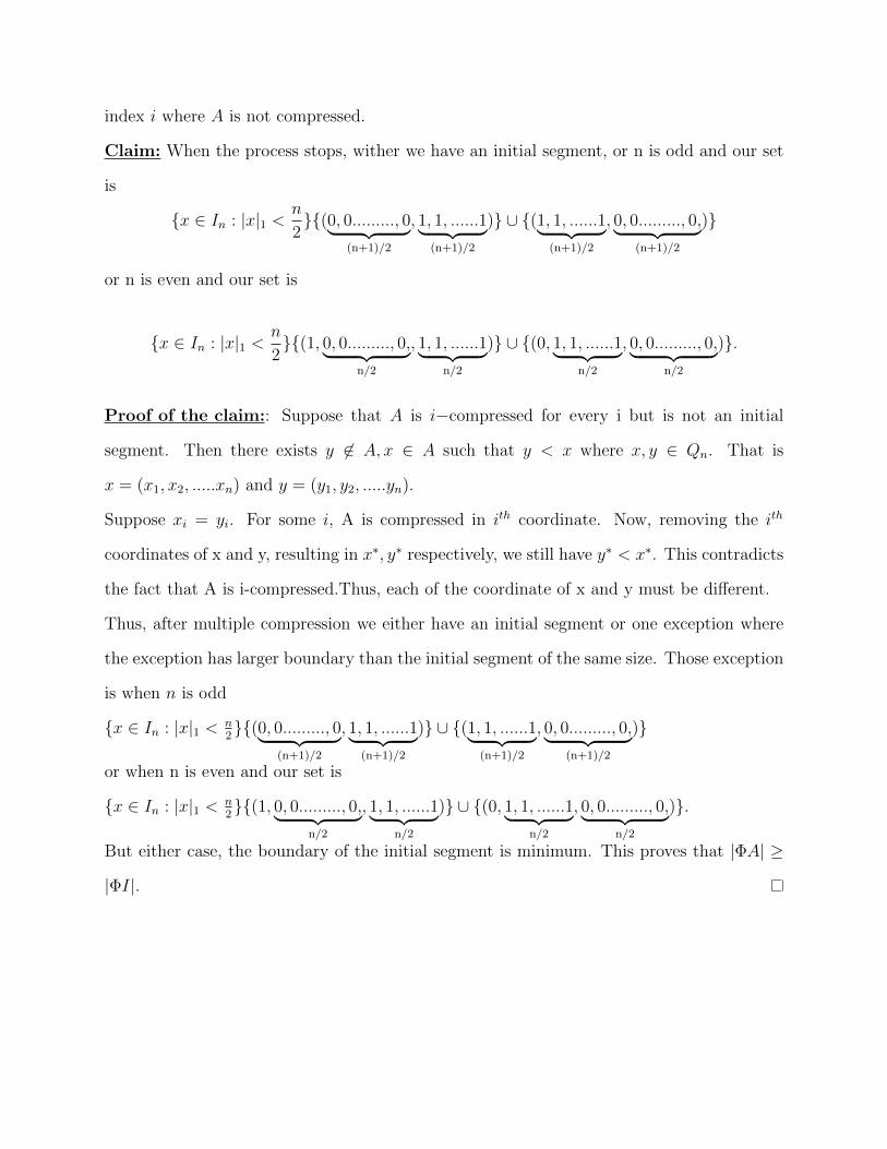
Theorem 2. (Harper’s Theorem)Let A ⊂ Qn. Let I be an initial segment in the boolean cube

in the simiplicial ordering. If |I| = |A|, then |ΦA| ≥ |ΦI|.

Proof. Let A be a set which is a subset of the boolean cube Qn and fix index for 1 ≤ i ≤ n,

let Ai0 be a set of vectors (v1, v2, v3....vn−1) in Qn−1 such that (v1, v2, .....vi−1, 0, vi, ....vn−1) ∈

A. This means that if we insert 0 in between the (i−1)th and ith entries, the resulting vector

is in A. Note that Ai0 is in the Qn−1 dimension boolean cube.

Similarly,

let Ai1 be set of vectors (v1, v2, v3....vn−1) in Qn−1 such that (v1, v2, .....vi−1, 1, vi, ....vn−1) ∈ A.

This means that if we insert 1 in between the (i − 1)th and ith entries, the resulting vector

is A.

Similarly, Ai1 is also n− 1 dimension boolean cube.

For example, if A = {000, 011, 111, 101, 110, 001} where A ⊂ Qn then,

A10 = {00, 11, 01} where we remove 0 from the 1st index.

Figure 10: A Simplicial ordering of Q4

A11 = {11, 01, 10} where we remove 1 from the 1st index.

Now, we define Ci which is the i-compression of A by taking Qn−1 dimension and fixing

the ith coordinate such that |(Ci)i0| = |Ai0| and (Ci)i0 is an initial segment in Qn−1 and

|(Ci)i1| = |Ai1| and (Ci)i1 is an initial segment in Qn−1. Now we note that,

(ΦA)i0 = Φ(Ai0) ∪ Ai1

(ΦCi)i0 = Φ((Ci)i0) ∪ (Ci)i1

Here, ΦCi)i0 is either equal to Φ((Ci)i0) or (Ci)i1 because the boundary of an initial segment

is itself an initial segment. So, for Φ(Ci) = Φ(Ci)0i ∪ Φ(Ci)i

1 both the boundaries for (Ci)0i

and (Ci)1i are disjoint. And similarly, for Φ(A) = Φ(A)0i ∪ Φ(A)1i both the boundaries

for (A)0i and (A)1i are disjoint. This follows by our definition, that |(Ci)i1| = |Ai1 | and

|(Ci)i0| = |Ai0|. Also, (Ci)i0 is the initial segment in Qn−1. Since, So by induction we have,

|Φ(Ci)i1| ≤ |Φ(Ai1)| and |Φ(Ci)i0| ≤ |Φ(Ai0)|.

We continue to do compression in the ith, we move onto another index i + 1 and perform

compression until A is compressed. After doing multiple compression in every coordinate,

the process must stop and the result with be either A is the initial segment or there is some

index i where A is not compressed.

Claim: When the process stops, wither we have an initial segment, or n is odd and our set

is

{x ∈ In : |x|1 <n

2}{(0, 0........., 0︸ ︷︷ ︸

(n+1)/2

, 1, 1, ......1︸ ︷︷ ︸(n+1)/2

)} ∪ {(1, 1, ......1︸ ︷︷ ︸(n+1)/2

, 0, 0........., 0,︸ ︷︷ ︸(n+1)/2

)}

or n is even and our set is

{x ∈ In : |x|1 <n

2}{(1, 0, 0........., 0,︸ ︷︷ ︸

n/2

, 1, 1, ......1︸ ︷︷ ︸n/2

)} ∪ {(0, 1, 1, ......1︸ ︷︷ ︸n/2

, 0, 0........., 0,︸ ︷︷ ︸n/2

)}.

Proof of the claim:: Suppose that A is i−compressed for every i but is not an initial

segment. Then there exists y 6∈ A, x ∈ A such that y < x where x, y ∈ Qn. That is

x = (x1, x2, .....xn) and y = (y1, y2, .....yn).

Suppose xi = yi. For some i, A is compressed in ith coordinate. Now, removing the ith

coordinates of x and y, resulting in x∗, y∗ respectively, we still have y∗ < x∗. This contradicts

the fact that A is i-compressed.Thus, each of the coordinate of x and y must be different.

Thus, after multiple compression we either have an initial segment or one exception where

the exception has larger boundary than the initial segment of the same size. Those exception

is when n is odd

{x ∈ In : |x|1 < n2}{(0, 0........., 0︸ ︷︷ ︸

(n+1)/2

, 1, 1, ......1︸ ︷︷ ︸(n+1)/2

)} ∪ {(1, 1, ......1︸ ︷︷ ︸(n+1)/2

, 0, 0........., 0,︸ ︷︷ ︸(n+1)/2

)}

or when n is even and our set is

{x ∈ In : |x|1 < n2}{(1, 0, 0........., 0,︸ ︷︷ ︸

n/2

, 1, 1, ......1︸ ︷︷ ︸n/2

)} ∪ {(0, 1, 1, ......1︸ ︷︷ ︸n/2

, 0, 0........., 0,︸ ︷︷ ︸n/2

)}.

But either case, the boundary of the initial segment is minimum. This proves that |ΦA| ≥

|ΦI|.

5 Conclusion

Harper’s theorem for VIP allow us to avoid direct calculation to find the minimal boundary

on Φ(I) or Φ(A) which can get really messy. It is easier if our size of A is the size of a

Hamming ball |X(≤r)|. Both Lexicographic ordering and simplicial ordering helps us find

the minimum boundary for edge and vertex isoperimetric problems on Boolean cubes. The

solution to discrete edge Isoperimetric problem and vertex isoperimetric problem helps to

find solution in various areas such as wirelength problem, minimum path problem, bandwidth

problem and many more.

6 Acknowledgements

I would like to thank my advisor Dr. Ellen Veomett for the support, help and suggestions

throughout the writing of this paper.

References

[1] Cibulis, A. On Zenodorus’s problem, Latvia. (2004),

[2] Harper L.H. Global Methods for Combinatorial Isoperimetric Problems. Cambridge Stud-

ies in Advanced Mathematics 90, Cambridge Univ,. Press(2004)

[3] Leader Imre. Discrete Isoperimetric Inequalities Probabilistic Combinatorics and its Ap-

plications. Volume 44 (1991)

[4] Harper L.H.. Optimal numberings and isoperimetric problems on graphs, J. Combinato-

rial Theory I1966, 385-394