Unit 2: Systems of Linear Inequalities
22
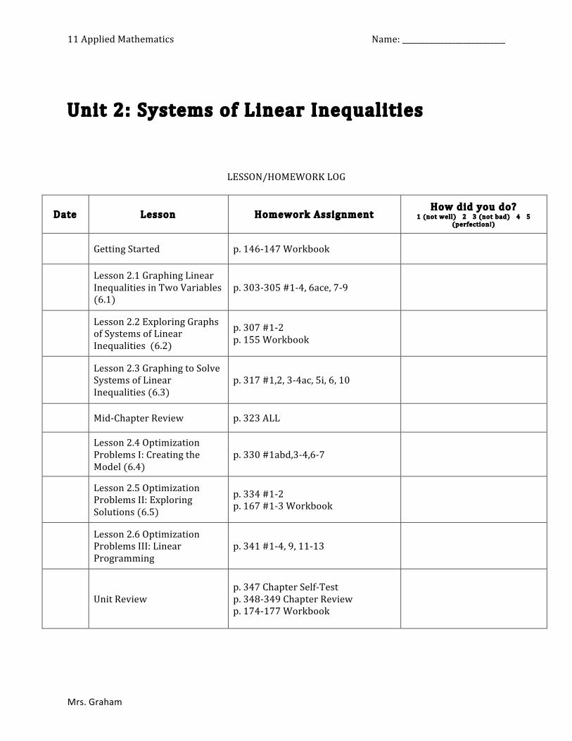
11 Applied Mathematics Name: ___________________________ Mrs. Graham Unit 2: Systems of Linear Inequalities LESSON/HOMEWORK LOG Date Lesson Homework Assignment How did you do? 1 (not well) 2 3 (not bad) 4 5 (perfection!) Getting Started p. 146147 Workbook Lesson 2.1 Graphing Linear Inequalities in Two Variables (6.1) p. 303305 #14, 6ace, 79 Lesson 2.2 Exploring Graphs of Systems of Linear Inequalities (6.2) p. 307 #12 p. 155 Workbook Lesson 2.3 Graphing to Solve Systems of Linear Inequalities (6.3) p. 317 #1,2, 34ac, 5i, 6, 10 MidChapter Review p. 323 ALL Lesson 2.4 Optimization Problems I: Creating the Model (6.4) p. 330 #1abd,34,67 Lesson 2.5 Optimization Problems II: Exploring Solutions (6.5) p. 334 #12 p. 167 #13 Workbook Lesson 2.6 Optimization Problems III: Linear Programming p. 341 #14, 9, 1113 Unit Review p. 347 Chapter SelfTest p. 348349 Chapter Review p. 174177 Workbook
-
Upload
khangminh22 -
Category
Documents
-
view
0 -
download
0
Transcript of Unit 2: Systems of Linear Inequalities
11 Applied Mathematics Name: ___________________________
Mrs. Graham
Unit 2: Systems of Linear Inequalities
LESSON/HOMEWORK LOG
Date Lesson Homework Assignment How did you do?
1 (not well) 2 3 (not bad) 4 5 (perfection!)
Getting Started p. 146-‐147 Workbook
Lesson 2.1 Graphing Linear Inequalities in Two Variables (6.1)
p. 303-‐305 #1-‐4, 6ace, 7-‐9
Lesson 2.2 Exploring Graphs of Systems of Linear Inequalities (6.2)
p. 307 #1-‐2 p. 155 Workbook
Lesson 2.3 Graphing to Solve Systems of Linear Inequalities (6.3)
p. 317 #1,2, 3-‐4ac, 5i, 6, 10
Mid-‐Chapter Review p. 323 ALL
Lesson 2.4 Optimization Problems I: Creating the Model (6.4)
p. 330 #1abd,3-‐4,6-‐7
Lesson 2.5 Optimization Problems II: Exploring Solutions (6.5)
p. 334 #1-‐2 p. 167 #1-‐3 Workbook
Lesson 2.6 Optimization Problems III: Linear Programming
p. 341 #1-‐4, 9, 11-‐13
Unit Review p. 347 Chapter Self-‐Test p. 348-‐349 Chapter Review p. 174-‐177 Workbook

11 Applied Mathematics
2

11 Applied Mathematics
3
Getting Started
Linear Inequality: A linear inequality is a relationship between two linear expressions in which one expression is less than (<), greater than (>), less than or equal to (≤), or greater than or equal to (≥) the other expression.
Set of Real Numbers:
Terms: Discrete Data:
_________________________________________________________________________________________________________
_________________________________________________________________________________________________________
Continuous Data: _________________________________________________________________________________________________________
_________________________________________________________________________________________________________
Independent Variable: _________________________________________________________________________________________________________
_________________________________________________________________________________________________________
Dependent Variable: _________________________________________________________________________________________________________
_________________________________________________________________________________________________________
11 Applied Mathematics
4
Solving Inequalities Rules The rules for inequalities are the same as those for equations with a couple extra. 1) If you multiply or divide an inequality by a negative you MUST REVERSE the inequality. Example: 2) If you invert an inequality, you must reverse the inequality provided both sides have the SAME SIGN . Example:

11 Applied Mathematics
5
11 Applied Mathematics
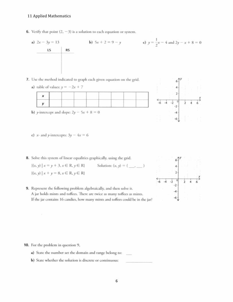
6
11 Applied Mathematics
7
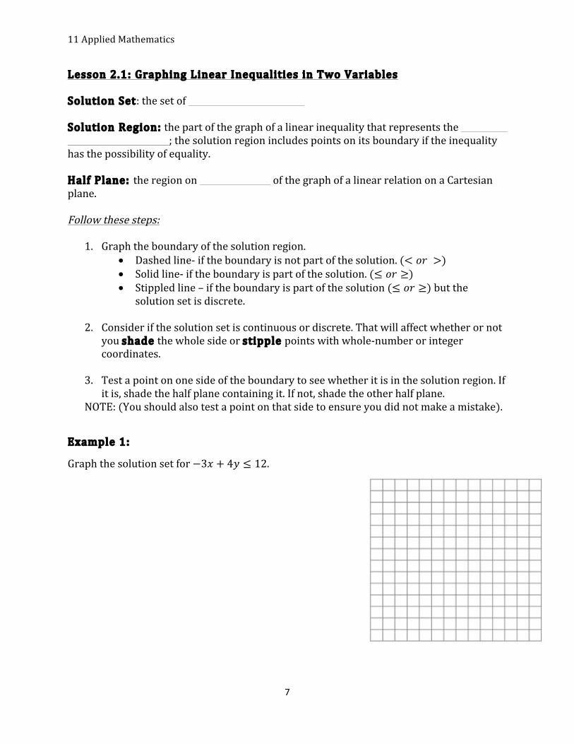
Lesson 2.1: Graphing Linear Inequalities in Two Variables
Solution Set: the set of Solution Region: the part of the graph of a linear inequality that represents the ; the solution region includes points on its boundary if the inequality has the possibility of equality. Half Plane: the region on of the graph of a linear relation on a Cartesian plane. Follow these steps:
1. Graph the boundary of the solution region. • Dashed line-‐ if the boundary is not part of the solution. (< 𝑜𝑟 >) • Solid line-‐ if the boundary is part of the solution. (≤ 𝑜𝑟 ≥) • Stippled line – if the boundary is part of the solution (≤ 𝑜𝑟 ≥) but the
solution set is discrete.
2. Consider if the solution set is continuous or discrete. That will affect whether or not you shade the whole side or stipple points with whole-‐number or integer coordinates.
3. Test a point on one side of the boundary to see whether it is in the solution region. If it is, shade the half plane containing it. If not, shade the other half plane.
NOTE: (You should also test a point on that side to ensure you did not make a mistake).
Example 1:
Graph the solution set for −3𝑥 + 4𝑦 ≤ 12.
11 Applied Mathematics
8
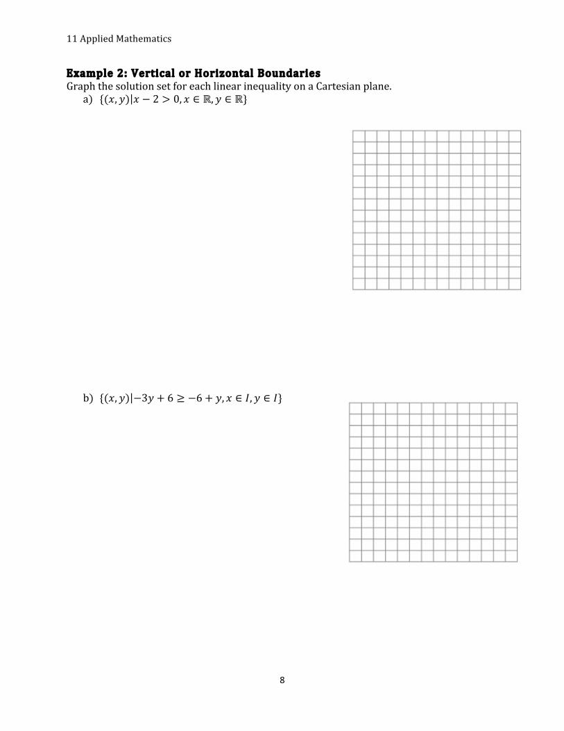
Example 2: Vertical or Horizontal Boundaries Graph the solution set for each linear inequality on a Cartesian plane.
a) {(𝑥,𝑦) 𝑥 − 2 > 0, 𝑥 ∈ ℝ,𝑦 ∈ ℝ}
b) {(𝑥,𝑦) −3𝑦 + 6 ≥ −6+ 𝑦, 𝑥 ∈ 𝐼,𝑦 ∈ 𝐼}

11 Applied Mathematics
9
Example 3: Solving a word problem A sports store has a net revenue of $100 on every pair of downhill skis sold and $120 on every snowboard sold. The manager’s goal is to have a net revenue of more than $600 a day from the sales of these two items. What combinations of ski and snowboard sales will meet or exceed this daily sales goal? Choose two combinations that make sense, and explain your choices. (*Use a graphing calculator to solve).

11 Applied Mathematics
10
Lesson 2.2: Exploring Graphs of Systems of Linear Inequalities
System of Linear Inequalities: a set of two or more linear inequalities that are graphed on the same coordinate plane; the of their solution regions represents the solution set for the system. NOTE: All of the inequalities in a system of linear inequalities are graphed on the same coordinate plane. The region where their solution regions represents the solution set to the system. Example 1: Graph this system of linear inequalities. Justify your representation of the solution set.
{(𝑥,𝑦) 𝑥 + 𝑦 ≤ 5, 𝑥 ∈ 𝐼,𝑦 ∈ 𝐼} {(𝑥,𝑦) 𝑥 + 3𝑦 > 0, 𝑥 ∈ 𝐼,𝑦 ∈ 𝐼}
11 Applied Mathematics
11
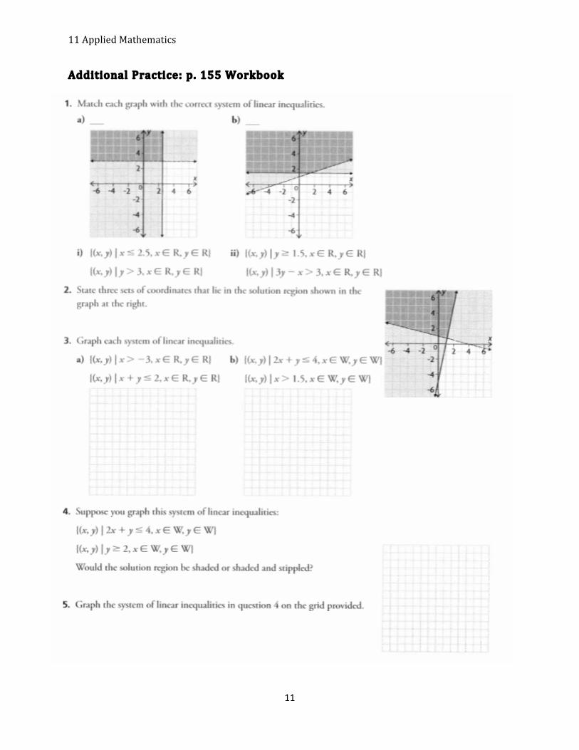
Additional Practice: p. 155 Workbook

11 Applied Mathematics
12
Lesson 2.3: Graphing to Solve Systems of Linear Inequalities Example 1: A company makes two types of boats on different assembly lines: aluminum fishing boats and fibreglass bow riders.
• When both assembly lines are running at full capacity, a maximum of 20 boats can be made in a day.
• The demand for fibreglass boats is greater than the demand for aluminum boats, so company makes at least 5 more fibreglass boats than aluminum boats each day.
What combinations of boats should the company make each day? Strategy 1: Use graph paper
11 Applied Mathematics
13
Strategy 2: Use graphing technology On Your Own: Graph the solution set for the following system of inequalities. State two possible solutions from the set. Check your work.
{(𝑥,𝑦) 2𝑥 + 𝑦 > 6, 𝑥 ∈𝑊,𝑦 ∈𝑊} {(𝑥,𝑦) 𝑦 ≤ 3, 𝑥 ∈𝑊,𝑦 ∈𝑊}

11 Applied Mathematics
14
Example 2: To raise funds to buy new instruments, the band committee has 500 T-‐shirts to sell. The T-‐shirts come in red or blue. Based on sales of the same T-‐shirts at a fundraiser five years ago, the committee expects to sell at least twice as many blue T-‐shirts as red T-‐shirts.
a) Define the variable and restrictions. Write a system of linear inequalities that models the situation.
b) Graph the system. (Use graphing technology). c) Suggest a combination of T-‐shirt sales that could be made.

11 Applied Mathematics
15
Lesson 2.4: Optimization Problems I: Creating the Model Optimization Problem: a problem where a quantity must be following a set of guidelines or conditions. Constraint: a of the optimization problem being modelled, represented by a linear inequality. Objective Function: in an optimization problem, the equation that represents the between the two variables in the system of linear inequalities and the quantity to be optimized. Feasible Region: the for a system of linear inequalities that is modelling an optimization problem. Steps to follow:
1. Identify the quantity that must be optimized. Look for key words such as maximize or minimize, largest or smallest, and greatest or least.
2. Define the variables that affect the quantity to be optimized. Identify any restrictions on these variables.
3. Write a system of linear inequalities to describe all the constraints of the problem. Graph the system.
4. Write an objective function to represent the relationship between the variables and the quantity to be optimized.
Example 1: Four teams are travelling to a baseball tournament in cars and minivans. Each team has no more than 3 coaches and 10 athletes. Each car can take 5 team members, and each minivan can take 8 team members. No more than 5 minivans and 11 cars are available. The school wants to know what combination of cars and minivans will require the maximum or minimum number of vehicles. Create and verify a model to represent this situation.
11 Applied Mathematics
16
Example 2: A refinery produces oil and gas.
• At least 2 L of gasoline is produced for each litre of heating oil. • The refinery can produce up to 9 million litres of heating oil and 6 million litres of
gasoline each day , • Gasoline is projected to sell for $1.10 per litre. Heating oil is projected to sell for
$1.75 per litre. The company needs to determine the daily combination of gas and heating oil that must be produced to maximize revenue. Create a model to represent this situation.

11 Applied Mathematics
17
Lesson 2.5: Optimization Problems II: Exploring Solutions Optimal Solution: a in the solution set that represents the maximum or minimum value of the objective function. The (points of intersection) of the feasible region represent the for the objective function. Example 1: Consider the model shown:
Restrictions: 𝑥 ∈ ℝ,𝑦 ∈ ℝ Constraints: 𝑥 + 3𝑦 ≤ 9, 𝑥 − 𝑦 ≤ 3, 𝑥 ≥ −3 Objective Function: 𝑃 = 2𝑥 + 𝑦
a) What point in the feasible region would result in the maximum value of the objective function? How could you have predicted this graphically?
b) What point in the feasible region would result in the minimum value of the objective function? How could you have predicted this graphically?
11 Applied Mathematics
18
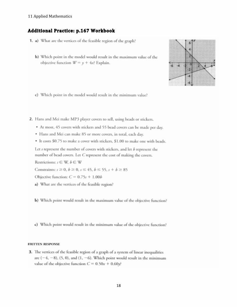
Additional Practice: p.167 Workbook

11 Applied Mathematics
19
Lesson 2.6: Optimization Problems III: Linear Programming Linear Programming: a used to determine which solutions in the feasible region result in the optimal solutions of the objective function. Example: Larry and Tony are baking cupcakes and banana mini-‐loaves to sell at a school fundraiser.
• No more than 60 cupcakes and 35 mini-‐loaves can be made each day. • Larry and Tony can make more than 80 baked goods, in total, each day. • It costs $0.50 to make a cupcake and $0.75 to make a mini-‐loaf.
They want to know the minimum costs to produce the baked goods.
11 Applied Mathematics
20

11 Applied Mathematics
21

11 Applied Mathematics
22