HAL Id: tel-03168284https://tel.archives-ouvertes.fr/tel-03168284

Submitted on 12 Mar 2021

HAL is a multi-disciplinary open accessarchive for the deposit and dissemination of sci-entific research documents, whether they are pub-lished or not. The documents may come fromteaching and research institutions in France orabroad, or from public or private research centers.

L’archive ouverte pluridisciplinaire HAL, estdestinée au dépôt et à la diffusion de documentsscientifiques de niveau recherche, publiés ou non,émanant des établissements d’enseignement et derecherche français ou étrangers, des laboratoirespublics ou privés.

Education policy, inequalities and student achievementAsma Benhenda

To cite this version:Asma Benhenda. Education policy, inequalities and student achievement. Political science. École deshautes études en sciences sociales (EHESS), 2020. English. �NNT : 2020EHES0044�. �tel-03168284�

Table des matieres

Remerciements 1

Resume de la these 3

Introduction Generale 5

1 Teacher Screening, On-the-Job Evaluations and Performance 21

1.1 Introduction . . . . . . . . . . . . . . . . . . . . . . . . . . . . . . . . . . . 21

1.2 Institutional Setting : Teacher Evaluations . . . . . . . . . . . . . . . . . . 25

1.3 Data and Summary Statistics . . . . . . . . . . . . . . . . . . . . . . . . . 29

1.4 How Efficient are Teacher Evaluations in Identifying Good Teachers ? . . . 33

1.5 What is the Impact of the Classroom Observation Evaluation on Teachers ? 39

1.6 Conclusion . . . . . . . . . . . . . . . . . . . . . . . . . . . . . . . . . . . 43

1.7 References . . . . . . . . . . . . . . . . . . . . . . . . . . . . . . . . . . . . 44

1.8 Tables and Figures . . . . . . . . . . . . . . . . . . . . . . . . . . . . . . . 48

1.9 Additional Tables and Figures . . . . . . . . . . . . . . . . . . . . . . . . 55

1.10 Data Appendix . . . . . . . . . . . . . . . . . . . . . . . . . . . . . . . . . 76

2 Absence, Substitutability and Productivity : Evidence from Teachers 83

2.1 Introduction . . . . . . . . . . . . . . . . . . . . . . . . . . . . . . . . . . . 83

2.2 Institutional Setting . . . . . . . . . . . . . . . . . . . . . . . . . . . . . . 87

2.3 Conceptual Framework . . . . . . . . . . . . . . . . . . . . . . . . . . . . . 90

2.4 Data and Descriptive Statistics . . . . . . . . . . . . . . . . . . . . . . . . 91

2.5 Empirical Strategy . . . . . . . . . . . . . . . . . . . . . . . . . . . . . . . 95

2.6 Baseline Results . . . . . . . . . . . . . . . . . . . . . . . . . . . . . . . . 97

2.7 Robustness Checks . . . . . . . . . . . . . . . . . . . . . . . . . . . . . . . 99

iii

2.8 Heterogeneity Analysis . . . . . . . . . . . . . . . . . . . . . . . . . . . . . 101

2.9 Conclusion . . . . . . . . . . . . . . . . . . . . . . . . . . . . . . . . . . . 104

2.10 Tables and Figures . . . . . . . . . . . . . . . . . . . . . . . . . . . . . . . 108

2.11 Detailed Conceptual Framework . . . . . . . . . . . . . . . . . . . . . . . 119

2.12 Data Appendix . . . . . . . . . . . . . . . . . . . . . . . . . . . . . . . . . 128

3 Stay a Little Longer ? Teacher Turnover, Retention and Quality in Di-

sadvantaged Schools 131

3.1 Introduction . . . . . . . . . . . . . . . . . . . . . . . . . . . . . . . . . . . 131

3.2 Institutional Setting . . . . . . . . . . . . . . . . . . . . . . . . . . . . . . 133

3.3 Data and Descriptive Evidence . . . . . . . . . . . . . . . . . . . . . . . . 136

3.4 Empirical Strategy . . . . . . . . . . . . . . . . . . . . . . . . . . . . . . . 142

3.5 Results . . . . . . . . . . . . . . . . . . . . . . . . . . . . . . . . . . . . . . 143

3.6 Conclusion . . . . . . . . . . . . . . . . . . . . . . . . . . . . . . . . . . . 145

3.7 References . . . . . . . . . . . . . . . . . . . . . . . . . . . . . . . . . . . . 146

3.8 Tables and Figures . . . . . . . . . . . . . . . . . . . . . . . . . . . . . . . 147

3.9 Appendix . . . . . . . . . . . . . . . . . . . . . . . . . . . . . . . . . . . . 165

iv

Remerciements

Mes annees de these ont ete des annees d’epanouissement intellectuel exceptionnel.

J’en sors avec la profonde volonte de continuer a me consacrer a la recherche et a l’analyse

des politiques publiques.

Je remercie d’abord Julien Grenet et Thomas Piketty, qui ont encadre cette these,

pour m’avoir transmis leur enthousiasme pour la recherche, et surtout pour une recherche

resolument ancree dans le debat public et motivee par les grandes questions. J’espere

pouvoir etre fidele a cette vision dans les annees a venir.

Il est difficile de resumer en quelques lignes ce que cette these doit a Julien. Il a

contribue a de nombreuses etapes de mon developpement intellectuel, et ceci bien avant

la these. Alors que j’entrais a peine a l’Ecole normale superieure de Cachan, il a pris le

temps de me former, avec un sens de la pedagogie hors norme. Je lui suis reconnaissante

de ne pas avoir compte son temps, pour son niveau d’exigence et de rigueur qui m’a pousse

a continuellement donner le meilleur de moi-meme. Je lui suis aussi reconnaissante pour

sa presence attentive tout au long de ces annees : j’ai partage avec lui mes succes, et,

surtout, j’ai toujours pu compter sur lui dans les nombreux moments de doutes, de gros

decouragement, et d’echecs cuisants qui egrenent la vie de thesarde. Je mesure difficilement

la chance que j’ai eue de le rencontrer si tot dans mon parcours, et suis heureuse de

continuer a travailler avec lui dans les annees a venir.

Je remercie Thomas pour son soutien et ses encouragements indefectibles et decisifs

tout au long de la these, et plus specifiquement lors des moments cruciaux qu’ont ete

mes sejours aux universites de Columbia et de Berkeley, ainsi pendant la periode critique

de transition vers le post-doc. Je le remercie de porter un agenda de recherche visant a

mieux comprendre les mecanismes generateurs d’inegalites : je me souviens bien de ma

lecture des Hauts revenus en France quand je n’etais qu’en prepa B/L : cette lecture a

fait partie de celles qui m’avaient convaincue de m’orienter vers l’economie.

1

Je tiens a adresser des remerciements tous particuliers a Jonah Rockoff. Mon sejour a

l’universite de Columbia sous sa direction a ete un tournant majeur de la these. Ses re-

marques et suggestions avisees tout au long de la these m’ont permis de considerablement

progresser. Je le remercie chaleureusement pour son soutien et ses encouragements.

Merci a Pauline Givord, Corinne Prost et Roland Rathelot pour avoir accepte de faire

partie du jury et pour avoir pris le temps de lire le manuscript de these. Leurs remarques

attentives m’ont ete tres utiles pour le finaliser.

Merci aux chercheurs du campus Jourdan et au-dela avec qui j’ai echange plus ponc-

tuellement : Marc Gurgand, mais aussi Luc Behaghel, Adrien Bouguen, Julien Combe,

Emma Duchini, Gabrielle Fack, Laurent Gobillon, Arthur Heim, Melina Hillion, Jesse

Rothstein, Arnaud Riegert, Camille Terrier et Clementine Van Effenterre.

Je remercie tous ceux qui m’ont permis de ne pas perdre de vue le lien entre recherche

et debat public. Merci a ceux qui ont participe a Regards croises sur l’economie entre

2011 et 2018 et plus specifiquement Claire Montialoux et Gabriel Zucman pour m’avoir

confie les clefs de cette maison que j’ai eue le plaisir de diriger pendant les annees de

these. Merci aussi a la DEPP : Catherine Moisan, pour avoir soutenu le projet de these

a ses tout debuts, mais aussi Cedric Afsa, Pierrette Briant, Caroline Simonis-Sueur et

Fabienne Rosenwald pour avoir facilite l’acces aux donnees, Caroline Caron et Sophie

Ruiz pour avoir partage leurs connaissances sur ces donnees, et Jean-Pierre Prudent pour

ses indications cruciales sur les bases SIRH. Merci a la Cour des comptes, et surtout a

Loıc Robert, pour avoir soutenu le projet sur les enseignants en Education prioritaire.

Merci a mes camarades jourdaniens pour leur bonne humeur : mes co-bureaux, Benja-

min, Helene, Luis, Martin, Nicolas, Quentin et Quitterie, mais aussi Alessandro, Aurelie,

Fanny, Jose, Marianne, Simon, et Yannick.

Merci enfin a mes proches : mon parcours et cette these doivent beaucoup a leur

confiance et soutien inconditionnels.

2

Resume de la these

Cette these analyse l’efficacite des dispositifs mis en place par la puissance publique

pour atteindre leurs trois principaux objectifs : attirer et retenir des enseignants de qua-

lite, aider les enseignants a s’ameliorer, et appareiller les enseignants a leurs eleves de facon

a reduire les inegalites educatives. Par rapport a l’essentiel de la litterature academique

existante consacree aux politiques educatives a destination des enseignants, cette these

elargit le champ d’analyse au role d’acteurs peu etudies dans la litterature : les jurys des

concours de recrutement, les inspecteurs d’academie et les chefs d’etablissement (chapitre

I), mais aussi les enseignants remplacants, qu’ils soient titulaires ou contractuels (chapitre

II). Elle etend enfin la discussion au systeme educatif dans son ensemble a travers l’ana-

lyse d’un mecanisme d’incitations non-monetaires mis en place pour attirer et retenir les

enseignants dans les etablissements defavorises (chapitre III).

Cette these commence par rappeler que le premier enjeu est, en amont, de mesurer

la qualite des enseignants. Si cette these confirme le role proeminent de l’experience des

enseignants, et met en avant celui de la note pedagogique et du statut de contractuel, il

semble cependant clair qu’aucun des indicateurs analyses ne permet, a lui seul, d’expliquer

les variations de qualite des enseignants. Les resultats de cette these vont ainsi dans le

sens de la litterature existante qui souligne qu’enseigner est une activite complexe et

multidimensionnelle, qui ne saurait se reduire a une seule et unique competence. En ce

qui concerne objectif au lui-meme de retention des enseignants de qualite, cette these

met en evidence le fait que les enseignants contractuels, recrutes ≪ sur le tas ≫ pour

assurer continuite de la qualite de l’enseignement en l’absence d’enseignant titulaire, ne

semblent pas etre mesure de remplir pleinement cette mission, que ce soit dans le contexte

d’affectation a l’annee ou de remplacements plus ponctuels.

Cette these souligne ensuite la difficulte a mettre en place des interventions efficaces

3

visant a aider les enseignants deja en poste a ameliorer leur performance. Si la note

d’inspection permet de capturer une dimension de la qualite des enseignants, l’inspection

elle-meme ne permet pas aux enseignants de progresser. Ce resultat contraste avec celui

de la litterature, qui met en evidence l’impact positif de dispositifs comparables, mais

beaucoup plus cibles et intensifs - et donc beaucoup plus couteux.

Cette these montre enfin que des mecanismes d’incitations non-monetaires existants

tels que le dispositif Affectation prioritaire a valoriser ne semblent pas avoir d’effet statis-

tiquement en termes de taux de mobilite ni de composition de la population enseignante

dans les etablissements defavorises, meme si ce dispositif permet de reduire les ecarts,

entre etablissements defavorises et les autres etablissements, de taux de sortie de la pro-

fession pour les enseignants inexperimentes. Reduire les inegalites dans la distribution

des enseignants entre les differents etablissements demeure donc un defi majeur pour la

puissance publique.

4

Introduction Generale

Cette these part du constat suivant : les enseignants sont l’un des facteurs decisifs de

la reussite de leurs eleves. Le consensus au sein de la litterature existante est que d’im-

portantes variations existent entre les enseignants en termes de capacite a faire progresser

leurs eleves (aussi appelee ≪ valeur ajoutee ≫), et que ces variations ont des consequences

majeures, a court terme comme a long terme. A court terme, une difference d’un ecart-

type de valeur ajoutee se traduit par une difference d’environ 10 % d’ecart-type dans le

progres de leurs eleves aux tests standardises de competences (Chetty et al., 2014a). A

long terme, les eleves affectes a des enseignants a forte valeur ajoutee ont plus de chance

de faire des etudes superieures et de beneficier de salaires plus eleves (Chetty et al., 2014b).

Ce constat souleve deux questions qui constituent la problematique de la these.

Premierement, il est crucial de mieux comprendre ce qui fait un bon enseignant :

quels sont les principaux determinants de la qualite des enseignants ? Il n’existe pas en-

core de reponse claire a cette question. Les principales pistes explorees, tels que le niveau

de diplome ou la certification, ne sont pas concluantes (Kane et al., 2008). Seules les

premieres annees d’experience expliquent de facon significative les ecarts de performance

entre les enseignants : l’ecart d’experience entre un enseignant sans aucune experience

et un enseignant plus experimente peut expliquer entre 5 et 10 % de la valeur-ajoutee

des enseignants (Rivkin et al., 2005). Cet effet se concentre cependant sur les premieres

annees : au-dela de ces cinq premieres annees, l’experience ne permet plus d’expliquer les

differences de valeur ajoutee (Rockoff, 2004). Deuxiemement, il est essentiel d’identifier les

politiques publiques susceptibles d’ameliorer la qualite des enseignants. Aux Etats-Unis,

la principale solution proposee consiste a lier directement des decisions majeures de res-

sources humaines telles que la promotion ou le licenciement des enseignants a des mesures

de valeur ajoutee (Green et al., 2012). Cette approche est neanmoins tres controversee

5

et fait l’objet de debats methodologiques (Rothstein, 2016) et politiques (McNeil, 2012)

importants.

Ces deux questions sont lourdes d’enjeux en termes de politique publique : en moyenne,

les pays de l’OCDE consacrent 5 % de leur PIB aux depenses educatives, et plus de

80 % des depenses educatives de fonctionnement sont attribuees a la remuneration des

personnels. En France, 65 milliards d’euros par an sont dedies a la remuneration des en-

seignants, soit plus de 3 % du PIB (OCDE, 2018). Ces depenses ne sont pas reparties

de facon egale sur le territoire : d’apres nos calculs, le salaire moyen brut des ensei-

gnants des etablissements publics les plus favorises est 10 a 15 % superieur a celui des

enseignants des etablissements les moins favorises (Benhenda, 2019). Ces disparites sont

essentiellement dues a des differences de composition de la population enseignante entre

ces etablissements. Par exemple, en 2014, l’experience moyenne des enseignants dans les

etablissements de l’Education prioritaire les plus defavorises est de 11 ans contre plus de

14 ans hors Education prioritaire (Benhenda, 2018). La proportion d’enseignants de moins

de 35 ans est, en 2015, de 38 % dans les etablissements d’Education prioritaire les plus

defavorises contre 24 % hors Education prioritaire (Dgesco, 2015). Ce phenomene est com-

mun a beaucoup d’autres pays developpes (OCDE, 2018). Aux Etats-Unis par exemple, le

nombre moyen d’annees d’experience des enseignants en sciences dans les etablissements

les plus defavorises est de 11,5 annees contre 15,5 annees dans les etablissements les plus

defavorises. Cela a des consequences considerables en termes d’inegalites de reussite sco-

laire : l’ecart de qualite des enseignants entre les etablissements favorises et defavorises

represente 20 % des inegalites de reussite scolaire entre les eleves de ces etablissements

(US Department of Education, 2013).

A cela s’ajoute le fait que la plupart des pays developpes font face a une crise majeure

de recrutement. D’apres l’OCDE (2018), ≪ la penurie d’enseignants est l’un des problemes

les plus urgents auxquels font face les systemes educatifs ≫. En France, le nombre d’ad-

mis aux concours enseignants du second degre public en 2016 est inferieur de 13 % aux

besoins de recrutement. Cette penurie touche principalement les mathematiques, ou 35 %

des postes au concours de l’Agregation et 20 % au CAPES ne sont pas pourvus (DEPP,

2016). Dans ce contexte, ameliorer, ou meme maintenir, la qualite de l’enseignement est

6

un defi delicat, surtout dans les etablissements les plus defavorises.

Face a ce defi, la contribution de cette these est d’analyser l’efficacite des dispositifs mis

en place par la puissance publique pour atteindre leurs trois principaux objectifs : ≪ attirer

et retenir des enseignants de qualite, aider les enseignants a s’ameliorer, et appareiller les

enseignants a leurs eleves de facon a reduire les inegalites educatives ≫ (OCDE, 2018). Par

rapport a l’essentiel de la litterature academique existante sur les politiques educatives a

destination des enseignants, cette these se propose de depasser le cadre d’analyse standard

qui se limite aux deux principaux protagonistes du systeme educatif : les enseignants

titulaires d’un cote, et leurs eleves, de l’autre. Ce cadre d’analyse ne met pas suffisamment

l’accent sur le fait que les enseignants font partie d’une organisation, avec de nombreux

acteurs et mecanismes, souvent presentes comme auxiliaires, mais qui peuvent en fait

jouer un role important dans la qualite de l’enseignement. Cette these elargit ainsi le

champ d’analyse au role d’acteurs peu etudies dans la litterature : les jurys des concours

de recrutement, les inspecteurs d’academie et les chefs d’etablissement (chapitre I), mais

aussi les enseignants remplacants, qu’ils soient titulaires ou contractuels (chapitre II). Elle

etend enfin la discussion au systeme educatif dans son ensemble a travers l’analyse d’un

mecanisme d’incitations non-monetaires mis en place pour attirer et retenir les enseignants

dans les etablissements defavorises (chapitre III).

Le recrutement des enseignants

Assurer la qualite de l’enseignement commence des le recrutement des enseignants

(chapitre I). Cette these analyse ainsi le role du jury des concours de recrutement des

enseignants du secondaire public a travers les notes qu’ils attribuent aux candidats. En

France, il existe deux principaux concours de recrutement pour les enseignants du secon-

daire public. Le premier est le CAPES (Certificat d’aptitude au professorat de l’enseigne-

ment du second degre). Les enseignants capetiens ont essentiellement vocation a enseigner

au college et au lycee. Le second est l’Agregation. Les agreges ont essentiellement voca-

tion a enseigner au lycee et en classe preparatoire aux grandes ecoles. Ces deux concours

se deroulent en deux etapes : un examen ecrit, puis, pour les candidats admissibles, un

examen oral. Les examens ecrits se composent de dissertations et de commentaires de do-

7

cuments en lettres et en histoire-geographie et d’exercices en mathematiques. Les examens

oraux se decomposent en trois parties : lecon, entretien et analyse de texte ou exercices

pour les mathematiques.

Deux specificites de ce concours en font un objet d’analyse particulierement pertinent

par rapport aux resultats de la litterature existante sur l’effet de la certification sur la

qualite des enseignants (Koedel et al., 2015). Premierement, le concours francais est plus

selectif que le processus de certification aux Etats-Unis, auquel l’essentiel de la litterature

est consacree. C’est particulierement le cas pour l’Agregation, dont une part significative

de candidats sont issus des Grandes Ecoles, et dont le taux d’admission a l’Agregation est

de 15 % contre plus de 30 % pour le CAPES (Depp, 2016). Deuxiemement, la specificite

du concours francais est sa dimension tres academique : il vise avant tout a evaluer les

connaissances de contenu des candidats plutot que leur savoir-faire pedagogique. Cela

permet ainsi d’analyser, en creux, la contribution des connaissances academiques a la

qualite des enseignants.

L’evaluation des enseignants

Une fois que les enseignants sont en poste, deux principaux acteurs sont en charge

de mesurer leurs performances et de les aider a progresser : le chef d’etablissement et

les inspecteurs d’academie. Les chefs d’etablissement evaluent leurs enseignants tous les

ans. Chaque annee, au mois de janvier, les chefs d’etablissement redigent un rapport sur

leurs enseignants, ou ils les evaluent en fonction de plusieurs criteres : ponctualite (etre

a l’heure, respecter les echeances) ; assiduite (pas d’absences injustifiees) ; efficacite (ini-

tiative, organisation, jugement), autorite (prise de decision, sens des responsabilites) et

influence (participation a des activites extra-scolaires, interactions avec les collegues). Ils

evaluent egalement les enseignants de facon quantitative en leur attribuant une note sur

40, appelee note administrative. La principale originalite de la notation des enseignants

par les chefs d’etablissements en France par rapport a ses equivalents a l’etranger est son

faible enjeu en termes de carriere. Contrairement a d’autres pays comme les Etats-Unis

(Jacob et Lefgren, 2008), le chef d’etablissement ne prend pas de decisions de ressources

humaines (recrutement, licenciement, promotion, etc.) car le systeme educatif francais

8

est tres centralise. L’analyse menee dans cette these permet donc egalement de contri-

buer au debat sur la decentralisation du systeme educatif qui donnerait plus de pouvoir

decisionnaire au chef et ses consequences en termes de qualite des enseignants (voir Eyles

et Machin (2015) pour le debat sur ≪ l’academisation ≫ au Royaume-Uni par exemple).

Une autre specificite de la note administrative par rapport aux evaluations etudiees

dans la litterature est qu’il est explicitement demande aux chefs d’etablissement de donner

≪ une appreciation sur la maniere de servir de l’enseignant, en dehors d’appreciation a

caractere pedagogique ≫. L’objectif de cette recommandation est que la note administra-

tive soit complementaire avec la note d’inspection, donnee par les inspecteurs d’academie.

Les inspecteurs d’academie sont des cadres superieurs de l’Education nationale, en general

d’anciens enseignants. Leur principale mission est de veiller a la mise en œuvre de la po-

litique educative dans les classes et les etablissements, et d’inspecter les personnels ensei-

gnants. A notre connaissance, il n’existe aucune etude consacree a l’efficacite du processus

d’inspection en France, malgre le fait que des ressources significatives y soient consacrees :

il existe environ 3 000 inspecteurs, avec un salaire brut mensuel de 3 600 euros. Le pro-

cessus d’inspection se deroule en trois grandes etapes. La premiere est la preparation de

cette visite par l’inspecteur. L’inspecteur a acces a l’ensemble des supports pedagogiques

de l’enseignant (cours, cahiers des eleves, etc.) ainsi qu’a ses precedentes evaluations

(notes d’inspection et notes administratives). Puis l’inspecteur se rend dans la classe de

l’enseignant pour observer un ou plusieurs de ses cours. Enfin, l’inspecteur fait un retour

individuel a l’enseignant et lui prodigue des conseils pour progresser.

L’objectif de ce processus est double : evaluer les enseignants, mais aussi leur fournir

un soutien pedagogique et un retour precis sur leur travail afin de leur donner les outils

necessaires pour progresser. Cette these analyse l’efficacite du processus d’inspection en

fonction de ses deux objectifs. L’essentiel de la litterature existante consacree au processus

d’evaluation s’interesse a des dispositifs tres localises, intenses et souvent dans des envi-

ronnements controles. Ils mettent en evidence pour l’essentiel l’efficacite de ces dispositifs

a mesurer la qualite des enseignants (Kane et al., 2011) et a les aider a progresser (Taylor

et Tyler, 2012). La contribution de cette these est de s’interesser a un dispositif national,

a grande echelle et peu intense. Par cette analyse, cette these contribue aussi en creux au

debat sur la difficulte d’elargir l’echelle de dispositifs efficaces mais tres locaux.

9

Les enseignants remplacants

Le dernier type d’acteurs auquel se consacre cette these sont les enseignants rem-

placants, dont la fonction premiere est d’assurer la continuite de l’enseignant en l’absence

de l’enseignant titulaire. Il existe deux types d’enseignants remplacants, de statuts et

niveaux de qualification differents : les enseignants titulaires sur zones de remplacement

(TZR) et les enseignants contractuels. Les enseignants TZR sont des enseignants titu-

laires, certifies ou agreges, mis en reserve et a la disposition du rectorat pour effectuer

des remplacements sur une zone geographique definie appelee zone de remplacement. Les

enseignants TZR, qui representent environ 15 % de la population enseignante (Benhenda,

2018), ont des caracteristiques observables tres comparables aux autres enseignants titu-

laires, a l’exception du fait qu’ils sont en moyenne moins experimentes : les enseignants

TZR ont en moyenne 10 annees d’experience contre 14 annees pour les autres enseignants

titulaires. Face au manque d’attractivite de la profession enseignante, l’Education natio-

nale a recours de facon de plus en plus perenne aux enseignants contractuels. Ces derniers

sont recrutes directement par les academies via une procedure distincte de celle employee

pour recruter les enseignants titulaires. Les candidats postulent directement sur une pla-

teforme en ligne. Il y a deux conditions d’eligibilite : etre titulaire d’une licence et ne pas

avoir de casier judiciaire. Les candidats selectionnes sont recrutes sur la base d’un contrat

a duree determinee d’une duree maximale d’un an. En 2016-2017, les enseignants contrac-

tuels representent environ 7 % de la population enseignante. Leur poids dans la population

enseignante est en forte croissance ces dernieres annees. En 2016-2017, la croissance an-

nuelle du nombre d’enseignants de titulaire est de 1 % tandis que celle des enseignants

contractuels est de 10 % (DEPP, 2018). Il existe de fortes disparites geographiques dans

la presence de contractuels, meme au sein d’une meme academie : ainsi dans l’academie

de Creteil, le taux de contractuels est de 13,7 % dans le departement de Seine Saint-Denis

contre 7,7 % en Seine-et-Marne (Cour des comptes, 2018). Dans les etablissements les plus

defavorises de l’Education prioritaire, plus de 16 % des enseignants sont des contractuels

(Benhenda, 2018).

Ce phenomene n’est pas propre a la France mais touche de nombreux pays developpes

(OCDE, 2018). En Italie, les enseignants non-titulaires representent 26 % de la population

enseignante dans etablissements defavorises contre seulement 12 % dans les etablissements

10

les plus favorises. Dans l’etat americain du Massachussetts, seulement 2,7 % des ensei-

gnants sont contractuels dans les etablissements les plus favorises contre plus de 12.5 %

dans les etablissements les plus defavorises.

Malgre l’importance de ce phenomene, qualifie par la Cour des comptes de ≪ d’enjeu

desormais significatif pour l’Education nationale ≫, il existe tres peu de travaux consacres

a l’effet des enseignants contractuels sur les performances de leurs eleves. La principale

etude existante porte sur le contexte tres specifique d’un pays en developpement, ou le

systeme de gestion des enseignants titulaires est defaillant, et ou les enseignants contrac-

tuels ont un niveau de qualification comparable aux titulaires et sont etroitement controles

(Duflo et al., 2015). La contribution de cette these est donc de s’interesser a un pays

developpe, la France, ou le contexte tres different : les contractuels sont en general re-

crutes sur le tas, avec des criteres d’eligibilite minimaux et sans vraiment de mecanismes

incitatifs une fois qu’ils sont en poste.

Attirer et retenir les enseignants dans les

etablissements defavorises

La derniere contribution de cette these elargit la focale : elle passe d’une analyse

d’acteurs a l’analyse d’un dispositif centralise visant a influencer les comportements de ces

acteurs et ainsi ameliorer leur allocation entre les differents etablissements. Ce dispositif

a pour objectif de pallier le fait que les eleves des etablissements defavorises sont plus

susceptibles de faire face a une forte instabilite des equipes enseignantes. En moyenne,

les enseignants affectes aux etablissements les plus defavorises de l’Education prioritaire

passent six annees consecutives dans le meme etablissement, contre plus de huit ans hors

Education prioritaire, soit un ecart de 25 %. Le taux de mobilite inter-etablissement

dans les etablissements hors Education prioritaire est de moins de 5 % contre plus de

10 % en Education prioritaire (Benhenda, 2018). Cette forte instabilite des equipes peut

affecter negativement les performances des eleves a travers deux principaux mecanismes.

Le premier est un effet de composition, lorsque les meilleurs enseignants sont les plus

susceptibles de quitter ces etablissements (Adnot et al., 2017). Le second est lie a l’effet

perturbateur et la perte de capital humain specifique a l’etablissement provoque par cette

instabilite (Ronfeldt et al., 2013).

11

Le principal dispositif analyse par la litterature pour faire face a ce phenomene est un

systeme de compensation financiere pour les enseignants affectes dans les etablissements

defavorises. Les etudes existantes ne permettent pas de conclure sur leur efficacite : cer-

taines, se focalisant plus specifiquement sur les Etats-Unis (Feng et Sass, 2016), mettent

en evidence un effet positif de ces dispositifs sur la qualite des enseignants et la stabilite

des equipes, tandis que d’autres, analysant le contexte francais (Prost, 2013) ne trouvent

pas d’effets statistiquement significatif. Par ailleurs, de nombreux elements suggerent que

les enseignants sont tres sensibles aux dimensions non pecuniaires de leurs conditions de

travail (Hanushek et al., 2004 ; Worth et al., 2018).

Cette these se propose ainsi d’analyser un dispositif centralise et d’incitations non

monetaires visant a attirer et retenir les enseignants dans les colleges publics defavorises,

baptise ≪ Affectation a caractere prioritaire justifiant une valorisation ≫ (APV). En

France, l’affectation des enseignants est realisee au moyen d’une procedure informatique

centralisee : les enseignants soumettent en ligne une liste hierarchisee de vœux puis sont af-

fectes selon une version modifiee de l’algorithme d’acceptation differee de Gale et Shapley

(Combe et al., 2018). Les principaux criteres definissant l’ordre de priorite des enseignants

sont la situation familiale, l’experience professionnelle (nombre d’annees depuis l’entree

dans la profession enseignante), l’anciennete (nombre d’annees consecutives passees dans

le meme etablissement), et l’anciennete en etablissement classe APV, souvent egalement

classe Education prioritaire. L’objectif de cette etude est ainsi d’evaluer l’efficacite du bo-

nus APV a atteindre ses deux principaux objectifs, tels qu’ils sont presentes dans les textes

officiels : ≪ rendre plus attractives les affectations a caractere prioritaire ≫ et ≪ d’inciter

[les enseignants] a s’investir durablement pour une periode d’au moins cinq ans ≫.

Plan de la these et principaux resultats

Cette these s’articule autour de trois parties. La premiere analyse le lien entre les notes

des enseignants aux concours de recrutement, la note donnee par le chef d’etablissement

(appelee note administrative) et la note d’inspection d’une part, et la capacite des ensei-

gnants a faire progresser leurs eleves d’autre part. La deuxieme partie s’interesse a l’effet

des absences et remplacements des enseignants sur les performances scolaires de leurs

eleves. Enfin, la troisieme partie analyse l’efficacite du dispositif Affectation prioritaire a

12

valoriser a attirer et retenir les enseignants dans les etablissements les plus defavorises.

L’ensemble de cette these s’appuie sur des donnees administratives exhaustives fournies

par la Direction de l’evaluation, de la prospective et de la performance du ministere de

l’Education nationale (MENJ-DEPP).

Chapitre I

Ce chapitre s’appuie sur des donnees qui incluent des informations sur les enseignants

telles que leur identifiant national, leur matiere, leur niveau de certification, leur ni-

veau d’experience, leur etablissement d’affectation, ainsi que leurs notes aux concours,

leurs notes administratives et d’inspection. Ces donnees incluent egalement des infor-

mations sur les eleves telles que leur identifiant individuel crypte, leurs caracteristiques

sociodemographiques, ainsi que leurs notes aux epreuves ecrites du Diplome national du

brevet (DNB) et du Baccalaureat.

Pour identifier le lien entre les notes d’evaluation des enseignants et leur capacite a

faire progresser leurs eleves, ce chapitre exploite les variations inter-matieres et intra-eleve

(pour un eleve donne) du nombre de jours d’absence et le nombre de jours de remplace-

ment. Il s’agit d’exploiter le fait que chaque eleve de troisieme a plusieurs enseignants au

cours de l’annee et que ses performances scolaires sont mesurees separement dans plusieurs

matieres a la fin de l’annee, via les epreuves du DNB. De ce fait, chaque annee, chaque

eleve est observe avec plusieurs enseignants, un par matiere. La methode ici employee

consiste a faire le lien, pour chaque eleve, entre les evaluations relatives de ses differents

enseignants et ses performances relatives dans les differentes matieres des epreuves finales

du brevet (francais, mathematiques, histoire-geographie). A niveau scolaire donne, les

eleves obtiennent-ils de moins bons resultats dans une matiere donnee, par rapport aux

autres matieres, quand l’enseignant de la matiere consideree a de meilleures evaluations

que les autres enseignants de l’eleves dans les autres matieres ? Le principal objectif de

cette approche (effets fixes eleves) est de neutraliser l’effet des determinants inobservables

des performances scolaires, consideres comme constants entre matieres, qui peuvent etre

correles aux evaluations des enseignants.

Deux principaux resultats emergent de cette analyse. Premierement, la note d’ins-

pection est la seule note d’evaluation liee de facon statistiquement significative aux per-

formances des enseignants. La magnitude de ce lien est tres faible : une difference d’un

13

ecart-type dans la note d’inspection est associee a une augmentation de 2 % d’ecart-type

des performances des eleves. Ce lien entre note pedagogique et qualite des enseignants

est plus fort pour les eleves issus de famille a faible revenu que pour les autres. Le statut

d’agrege, les notes aux concours (ecrit comme oral) ou la note du chef d’etablissement ne

semblent pas, quant a eux, etre lies de facon statistiquement significative a la qualite des

enseignants.

Deuxiemement, l’inspection ne semble avoir aucun effet durable sur les performances

des enseignants. L’annee de l’inspection, les enseignants sont legerement moins absents.

Ainsi, si l’inspection semble atteindre partiellement son premier objectif, mesurer la qua-

lite des enseignants, elle ne semble pas etre en mesure d’atteindre son second objectif,

aider les enseignants a ameliorer leurs performances.

Chapitre II

La specificite des donnees exploitees dans ce chapitre par rapport a celles du chapitre

precedent est qu’elles contiennent des informations detaillees sur les conges des ensei-

gnants telles que la date precise de ces conges et leur motif, pour chaque enseignant. Elles

permettent egalement de faire le lien entre chaque conge et, le cas echeant, l’enseignant

qui a effectue le remplacement.

Pour identifier l’impact causal du nombre de jours d’absence et de remplacement des

enseignants sur les performances des eleves, ce chapitre combine la methode ≪ en coupe

≫ utilisee au premier chapitre (exploitation des variations inter-matieres et intra-eleves)

a une approche longitudinale : il s’agit d’exploiter le fait que chaque enseignant est ob-

serve plusieurs annees, et que son nombre de jours d’absence et de remplacement varie

d’une annee a une autre. La methodologie employee consiste a faire le lien, pour chaque

enseignant, entre ses variations dans le nombre d’absences et de remplacements et les va-

riations interannuelles des performances scolaires de ses eleves. Les annees ou l’enseignant

est davantage absent/moins souvent remplace correspondent-elles a des annees de moindre

performance pour ses eleves ? Le principal objectif de cette approche est de ≪ neutraliser

≫ les determinants inobservables de l’effet enseignant qui ne varient pas d’une annee a

une autre.

Cette analyse montre que les absences des enseignants ont un effet negatif et statis-

tiquement significatif sur les performances scolaires des eleves, quel que ce soit le type

14

d’etablissement considere. En moyenne, un jour supplementaire d’absence non remplace

reduit les performances scolaires des eleves d’environ de 0.02 % d’un ecart-type, ce qui est

comparable aux resultats mis en evidence par la litterature. Cet effet est statistiquement

significatif, meme s’il convient de souligner que sa magnitude est faible. L’effet moyen

de 10 jours d’absence non remplaces est en effet equivalent a un quart de l’effet d’une

augmentation de la taille des classes au college d’un eleve 1. Seuls les enseignants titulaires

sur zone de remplacement semblent avoir un effet compensateur statistiquement significa-

tif : un jour de remplacement par un titulaire sur zone de remplacement compense jusqu’a

25 % de l’impact negatif d’un jour d’absence non remplace sur les performances des eleves.

A l’inverse, les enseignants contractuels n’ont aucun effet compensateur statistiquement

significatif. Ce resultat suggere que les enseignants titulaires sur zone de remplacement

sont en mesure d’assurer une partie de la continuite de la qualite de l’enseignement,

contrairement aux enseignants contractuels.

Chapitre III

Les enseignants du secondaire sont affectes selon une procedure automatisee, qui prend

en compte un certain nombre de criteres tels que la situation familiale de l’enseignant, son

nombre d’annees d’experience et son anciennete dans l’etablissement (nombre d’annees

consecutives passees dans le meme etablissement). Le dispositif Affectation prioritaire a

valoriser (APV) consiste a attribuer des points de mobilite supplementaires aux ensei-

gnants qui ont ete affectes dans les etablissements ayant recus la classification APV, et

qui y ont exerce pendant plusieurs annees consecutives.

Afin d’evaluer ce dispositif, nous nous interessons a une reforme majeure de la struc-

ture de ce bonus en 2005. Avant 2005, les enseignants en APV commencaient a beneficier

d’un bonus a partir de trois ans d’anciennete. Apres 2005, la duree d’anciennete requise

est passee a cinq ans. La valeur du bonus APV a cinq ans d’anciennete est desormais

equivalente a la valeur du bonus experience pour un enseignant ayant accumule 43 ans

d’experience. Notre analyse suggere que cette reforme a permis d’augmenter de 0,3 annee

l’anciennete moyenne des enseignants exercant dans les etablissements concernes par la bo-

nification APV, par rapport aux enseignants affectes a des etablissements non concernes.

Une analyse plus fine nous permet d’observer que le principal effet de cette reforme est

1. voir Benhenda (2018) pour le detail de ce calcul.

15

que les enseignants ont plus tendance a rester dans leur etablissement APV jusqu’a 5 ans

d’anciennete, mais aussi a le quitter des qu’ils atteignent le nombre d’annees requises pour

beneficier de la bonification. Cette reforme a egalement permis de reduire la probabilite

des enseignants inexperimentes affectes a un etablissement APV de quitter la profession

enseignante.

Cette reforme n’a pas eu en revanche d’effet clair sur la composition des enseignants,

telle qu’elle est mesuree par leur nombre d’annees d’experience, ni sur les ecarts moyens

de performance scolaire des eleves (mesures par leurs notes standardisees aux epreuves

du DNB) entre les etablissements APV et les autres.

Principaux enseignements de la these

La principale contribution de cette these, comme enonce au debut de cette introduc-

tion, est d’analyser l’efficacite des dispositifs mis en place par la puissance publique pour

atteindre leurs trois principaux objectifs : i) attirer et retenir des enseignants de qualite ;

ii) aider les enseignants a s’ameliorer ; iii) appareiller les enseignants a leurs eleves de facon

a reduire les inegalites educatives. Au terme de l’analyse menee dans cette these, nous

mettons en evidence les conclusions pouvant etre tirees par rapport a ces trois objectifs.

Attirer et retenir enseignants de qualite

Cette these rappelle que le premier enjeu est, en amont, de mesurer la qualite des

enseignants. Si cette these confirme le role proeminent de l’experience des enseignants, et

met en avant celui de la note pedagogique et du statut de contractuel, il semble cependant

clair qu’aucun des indicateurs analyses ne permet, a lui seul, d’expliquer les variations de

qualite des enseignants. Les resultats de cette these vont ainsi dans le sens de la litterature

existante qui souligne qu’enseigner est une activite complexe et multidimensionnelle, qui

ne saurait se reduire a une seule et unique competence.

En ce qui concerne objectif de retention des enseignants de qualite, cette these met

en avant l’urgence de politiques plus ambitieuses pour l’atteindre. La France, comme

de nombreux autres pays developpes, souffre d’une crise de recrutement des enseignants

majeure. Cette crise a des consequences directes sur la qualite de l’enseignement : un

des principaux resultats de cette these est que les enseignants contractuels, recrutes sur

16

le tas pour assurer continuite de la qualite de l’enseignement en l’absence d’enseignant

titulaire, ne semblent pas etre mesure de remplir pleinement cette mission, que ce soit

dans le contexte d’affectation a l’annee ou de remplacements plus ponctuels.

Aider les enseignants a s’ameliorer

Cette these met en evidence la difficulte a mettre en place des interventions efficaces

visant a aider les enseignants deja en poste a ameliorer leur performance. Si la note

d’inspection permet de capturer une dimension de la qualite des enseignants, l’inspection

elle-meme ne permet pas aux enseignants de progresser. Ce resultat contraste avec celui

de la litterature, qui met en evidence l’impact positif de dispositifs comparables, mais

beaucoup plus cibles et intensifs - et donc beaucoup plus couteux.

Appareiller les enseignants a leurs eleves de facon a reduire les inegalites

educatives

Cette these fait tout d’abord le constat d’une inegale distribution des caracteristiques

observables des enseignants, telles que l’experience, entre les etablissements defavorises

et les autres. Aussi, dans les etablissements defavorises, les enseignants contractuels sont

surrepresentes, et les enseignants plus frequemment absents et moins remplaces.

Cette these montre ensuite que des mecanismes d’incitations non-monetaires exis-

tants tels que le dispositif APV ne semblent pas avoir d’effet statistiquement significatif

en termes de taux de mobilite ni de composition de la population enseignante dans les

etablissements defavorises, meme si ce dispositif permet de reduire les ecarts de taux de

sortie de la profession pour les enseignants inexperimentes. Reduire les inegalites de dis-

tribution des enseignants entre les differents etablissements demeure donc un defi majeur

pour la puissance publique.

Pour autant, la litterature internationale mentionnee dans cette these souligne que

lorsque les moyens alloues sont ambitieux, il est possible d’agir de facon significative

sur la composition de la population enseignante dans les etablissements defavorises. En

France, la question reste de savoir si les reformes recentes d’incitations monetaires dans

les etablissements de l’Education prioritaire sont a meme de relever ce defi. Un de nos

travaux en cours s’interesse a la reforme de l’Education prioritaire de 2015, dont l’un des

volets est d’augmenter la prime des enseignants dans ces etablissements de plus de 60 %,

17

la portant a pres de 3.500 euros par an dans les etablissements les plus defavorises de

l’Education prioritaire. Une analyse preliminaire suggere que cette reforme permet aux

salaires moyens dans les etablissements les plus defavorises d’etre equivalents a ceux des

enseignants dans les etablissements plus favorises. La question qui reste ouverte est de

savoir si cela est suffisant pour agir de facon consequente sur la composition enseignante

dans les etablissements les plus defavorises.

Bibliographie

Adnot, M., Dee, T., Katz, V., Wyckoff, J. (2017). Teacher turnover, teacher quality,

and student achievement in DCPS. Educational Evaluation and Policy Analysis, 39(1),

54-76.

Benhenda, A. (2018), Gestion des enseignants et inegalites scolaires dans les colleges

de l’education prioritaire, Paris School of Economics/Institut des politiques publiques,

Rapport pour la Cour des comptes, mai, 132 p.

Benhenda (2019). Teaching Staff Characteristics and Spending per Student in French

Disadvantaged Schools, Travail en cours.

Chetty, R., Friedman, J. N., & Rockoff, J. E. (2014a). Measuring the impacts of

teachers I : Evaluating bias in teacher value-added estimates. American Economic Review,

104(9), 2593-2632.

Chetty, R., Friedman, J. N., & Rockoff, J. E. (2014). Measuring the impacts of teachers

II : Teacher value-added and student outcomes in adulthood. American economic review,

104(9), 2633-79.

Combe J., Tercieux O. Terrier C. (2018). The Design of Teacher Assignment : Theory

and Evidence, Document de travail, Ecole d’economie de Paris.

Cour des comptes, 2018. Le recours croissant aux personnels contractuels, Communi-

cation a la commission des finances du Senat.

DEPP (2016). Concours Enseignants 2016 du Second Degre Public, Note d’informa-

tion, Ministere de l’Education nationale.

DEPP (2018). Les personnels du ministere de l’Education nationale en 2016-2017,

Note d’information, Ministere de l’Education nationale.

Dgesco (2015). Education prioritaire Tableau de bord national Donnees 2014-2015,

18

ministere de l’Education nationale.

Duflo, E., Hanna, R., Ryan, S. P. (2012). Incentives Work : Getting Teachers to Come

to School. The American Economic Review, 102(4) : 1241-1278.

Feng, L., Sass, T. R. (2016). The Impact of Incentives to Recruit and Retain Tea-

chers in “Hard-to-Staff” Subjects. Working Paper 141, National Center for Analysis of

Longitudinal Data in Education Research.

Green III, P. C., Baker, B. D., Oluwole, J. (2012). The legal and policy implications

of value-added teacher assessment policies. BYU Educ. LJ, 1.

Eyles A., Machin S. (2015), The Introduction of Academy Schools to England’s Edu-

cation, CEP Discussion Paper No. 1368.

Hanushek, E.A., Kain, J.F. Rivkin, S.G. (2004). Why Public Schools Lose Teachers.

Journal of Human Resources, 39(2), pp.326-354.

Jacob, B. A., Lefgren, L. (2008). Can principals identify effective teachers ? Evidence

on subjective performance evaluation in education. Journal of labor Economics, 26(1),

101-136.

Kane, T. J., Rockoff, J. E., Staiger, D. O. (2008). What does certification tell us about

teacher effectiveness ? Evidence from New York City. Economics of Education review,

27(6), 615-631.

Kane, T. J., Taylor, E. S., Tyler, J. H., Wooten, A. L. (2011). Identifying Effec-

tive Classroom Practices using Student Achievement Data. Journal of Human Resources,

46(3), 587-613.

Koedel, C., Parsons, E., Podgursky, M., Ehlert, M. (2015). Teacher preparation pro-

grams and teacher quality : Are there real differences across programs ? Education Finance

and Policy, 10(4), 508-534.

OCDE (2018), Effective Teacher Policies : Insights from PISA, PISA, OECD Publi-

shing, Paris.

Prost, C. (2013). Teacher mobility : Can Financial Incentives Help Disadvantaged

Schools to Retain their Teachers ?. Annals of Economics and Statistics, 171-191.

McNeil, M. (2012). Reports detail Race to Top winners’ challenges : States face diffi-

culties delivering on promises. Education Week. Retrieved from www.edweek.org.

Rivkin, S. G., Hanushek, E. A., & Kain, J. F. (2005). Teachers, schools, and academic

achievement. Econometrica, 73(2), 417-458.

19

Rockoff, J. E. (2004). The impact of individual teachers on student achievement :

Evidence from panel data. American economic review, 94(2), 247-252.

Ronfeldt, M., Loeb, S., Wyckoff, J. (2013). How teacher turnover harms student

achievement. American Educational Research Journal, 50(1), 4-36.

Rothstein, J. (2017). Measuring the Impacts of Teachers : Comment. American Eco-

nomic Review, 107 (6) : 1656-84.

Taylor, E.S. and Tyler, J.H. (2012). The effect of evaluation on teacher performance.

American Economic Review, 102(7), pp.3628-51.

Worth, J., Lynch, S., Hilary, J., Rennie, C., Andrade, J. (2018). Teacher Workforce

Dynamics in England. Slough :National Foundation for Educational Research.

20

Chapitre 1

Teacher Screening, On-the-Job

Evaluations and Performance

I study the relationship between systematic screening, on-the-job teacher evaluations,

and teacher performance in secondary school. Using comprehensive French administrative

data, I exploit within-student across subject variation and find that having a non-certified

teacher is associated with a 6 percent decrease in student achievement. Among certified

teachers, only the evaluation based on classroom observation is significantly related to

teacher performance. I then investigate whether classroom observation has an impact on

teacher performance and behaviour during the year of evaluation and in subsequent years.

An event study shows that classroom observation has no statistically significant impact on

student achievement nor on teachers’ probability to quit. I find that teachers are slightly

less likely to be absent during the year of the evaluation, suggesting that this evaluation

provokes a temporary change in teacher behaviour. JEL : I2, J2, M51.

1.1 Introduction

There is growing evidence showing substantial variation in teacher effectiveness (see

Koedel et al., 2015 for a review). However, there is still little evidence on how to identify

good teachers and how to improve teacher performance despite the considerable attention

researchers dedicate to this question. 1 This paper analyses teacher evaluations, one of the

main tools used by policy makers to solve this issue. How efficient are teacher evaluations

1. see Loyalka (2019) for a recent discussion

21

in identifying good teachers ? Do teacher evaluations have an impact on subsequent teacher

performance ?

A lot of public resources are devoted to evaluating teachers. In the United States for

example, evaluations can cost up to $4,000 per teacher each year. 2 Teacher evaluation is

widespread in many developed countries : across the OECD, more than 75 % of students

are enrolled in schools where teachers are evaluated (Isore, 2009). Because of the impor-

tance of this practice, more evidence on its efficiency is needed. The existing set of papers

on this question are conducted in very specific contexts, often in controlled environments,

with frequent, feedback intensive and high stake evaluations, which are not representative

of most teacher evaluation systems (see Steinberg and Donaldson, 2016 for a review).

This paper analyses the relationship among nationwide certification exams, on-the-job

teacher evaluations, and teacher performance in secondary school. I use administrative

data on 22,519 teachers and 502,302 students covering French public secondary schools

from 2006-2015. I analyse multiple evaluations, both before recruitment and on-the-job,

aiming at measuring potentially relevant dimensions of effective teaching : i) written and

oral certification exam scores, aimed at measuring content-knowledge ; ii) classroom ob-

servation grade by an external inspector, aimed at measuring pedagogical and relational

skills ; iii) school principal grade, aimed at measuring good behaviour outside the class-

room.

First, I examine the screening/accountability objective of teacher evaluation. How

efficient are teacher evaluations in identifying good teachers ? I exploit the fact that, in

secondary school, teachers are subject-specific to identify the relationship between teacher

evaluations and student achievement. I exploit within student, across subject variation in

teachers, and a fortiori in teachers’ evaluations, to identify their relationship with teacher

effectiveness in raising students’ test scores in 9th grade and 12th grade. I find that ha-

ving a non-certified teacher rather than a certified teacher is associated with a 6 percent

decrease in student achievement. Among certified teachers, I find neither the certifica-

tion level (high, called Agregation vs. basic, called CAPES), nor the certification grades

(written nor oral) are associated with student achievement gains, whether analysed se-

parately or jointly in a horse race with the other evaluation grades. I also find that the

2. This figure corresponds to the Cincinatti teacher evaluation system, see Taylor and Tyler (2012) formore details.

22

school principal grade is not statistically associated with student achievement, whatever

the specification. The only evaluation grade significantly associated with student achieve-

ment gains is the classroom observation grade. Both in 9th grade and 12th grade, a one

standard deviation increase in the classroom observation grade is associated with around

two percent of a standard deviation increase in student achievement gains. I find that low

income students are more sensitive to the classroom observation grade, especially in 12th

grade. I find no statistically significant heterogeneity by teacher experience.

Second, I analyse the human capital formation dimension. Do teacher evaluations

have an impact on subsequent teacher behaviour and performance ? I focus on classroom

observation because i) the previous analysis shows its corresponding grade is the only one

significantly related to teacher effectiveness ; ii) contrary to the school principal evaluation,

this evaluation does not occur every year, which allows me to conduct an event study. I

deal with endogeneity steming from non-random teacher - student matching with teacher

and classroom-year fixed effects. I start by analysing the impact of the evaluation on

teacher behaviour. The intuition I want to test is whether classroom observation and its

feedback have a motivating effect both at the extensive and intensive margins. I measure

the extensive margin with teachers’ probability to quit. To measure the intensive margin, I

follow the literature and use comprehensive administrative data on teacher absence spells

to measure effort (see Jacob, 2013 for a discussion). I find that classroom observation

has no statistically significant impact on the probability to quit. I find that teachers are

slightly less likely to be absent during the year of the evaluation, suggesting that this

evaluation provokes a temporary change on the intensive margin. To analyse the impact

of the evaluation on teacher performance, I study its impact on student achievement. I

find that the classroom observation has no statistically significant impact on student test

scores.

The contribution of this paper to the literature is twofold. First, it contributes to

the literature on teacher evaluations. This paper is globally consistent with the growing

evidence that classroom observations do predict student achievement gains (Kane et al.,

2013, Garret and Steinberg, 2015 ; Araujo et al., 2016, Bacher-Hicks et al., 2017, Jacob et

al., 2018). However, this paper is at odds with the literature showing that the classroom

observation has a positive impact on subsequent teacher performance (Taylor and Tyler,

2012). An important point to consider is, as mentioned above, most of the literature

23

analyses intensive, high stakes but small programs, focused on a few hundreds teachers.

These targeted programs are not representative of most existing evaluation systems. In

this paper, I study a nationwide program designed to handle the whole population of

secondary teachers in France (hundred of thousands of teachers). While the certification

exam is pretty high stakes, the two on-the-job evaluations are low stakes as they have

limited impact on teacher careers. This is different from the setting studied by Taylor

and Tyler (2012) where a successful evaluation is required to get tenure. Therefore, these

results have major implication for public policy since they highlight the challenges of

taking efficient but small programs to scale.

This paper also contributes to the literature on screening measures of effective tea-

ching. This literature mostly focuses on teacher certification in the United States (Kane,

Rockoff and Staiger, 2008) and finds that it is, at best, a very weak predictor of teacher

quality. While teacher certification in the United States is neither selective nor compe-

titive (Koedel, 2011), the certification process in France is academically demanding and

has low passing rates. This is particularly the case for the higher level of certification, the

Agregation, which draws applicants from the elite French Grandes Ecoles and universities

and has a passing rate of around 10 %. In that sense, this paper relates to the literature

on Teach for America, a highly selective program which recruits college graduates from

elite US universities to teach in low income areas. These papers find positive effects of

this program ( Boyd et al., 2006 ; Kane et al., 2008 ; Henry et al., 2014). While Teach for

America is an alternative certification program, focused on a small fraction of candidates,

the French certification process is government-run and the only way to become a tenured

and certified teacher. Furthermore, in this paper, I analyse not only the impact of the

certification level, but also of the precise certification test scores, at both stages (written

then oral) of the certification process. This relates this present paper to recent work which

uses detailed data on teacher applications to a centralized multi-stage application process

(Goldhaber et al., 2017 ; Jacob et al., 2016).

The remainder of this paper proceeds as follows. Section 2 provide a detailed descrip-

tion of the evaluations. Section 3 describes the data. Section 4 analyses the relationship

between teacher evaluations and student achievement. Section 5 studies the impact of the

classroom evaluation on teacher effort and performance. Section 6 discusses the results

and concludes.

24

1.2 Institutional Setting : Teacher Evaluations

1.2.1 Secondary School Teachers in France

The public French educational system is highly centralized. The French territory is

composed of 25 large administrative regions. Contrary to the United States for example,

schools have little autonomy : they are all required to follow the same national curriculum.

School principals cannot hire nor fire their teachers. Certified teachers are assigned via

a centralized point-based system. Candidates submit a rank-ordered list of choices and

are assigned according to a modified version of the school-proposing Deferred Acceptance

mechanism (Combes, Tercieux and Terrier, 2016).

Secondary school teachers are subject-specific : each subject is taught by a different

teacher. In 9th grade, students are not tracked by major nor ability. In 12th grade, students

are tracked by major, mainly hard science or social sciences. In both 9th and 12th grades,

students stay in the same class, with the same peers throughout the school year and in

every subject. At the end of 9th grade, students take a national and externally graded

examination called Diplome national du Brevet in three subjects : French, Math and

History. At the end of 12th grade, students take another national and externally graded

examination called Baccalaureat .

1.2.2 The Certification Process

Teacher certification is obtained after passing a competitive national examination. This

examination is taken after at least a year of intensive preparation at university depart-

ments specifically dedicated to teacher training. The examination for teaching in middle

school (college) or high school (lycee) is subject-specific. There are two main certification

levels for teachers teaching in secondary or high schools. The basic certification level is

called Certificat d’aptitude au professorat de l’enseignement du second degre (CAPES).

Basic certification recipients are essentially meant to teach in secondary school (which

includes 9th grade) or in high school (which includes 12th grade). The advanced certifi-

cation level is called Agregation. Advanced certification recipients are essentially meant

to teach in the academic track of high school (which includes 12th grade) and sometimes

in higher education, at the undergraduate level. 3 The advanced certification is more se-

3. The Certifie and Agrege statuses are defined, respectively, by the Decree n°72-581 of July 4, 1972and by the Decree n°72-580 of July 4, 1972.

25

lective than the basic one : for example, in mathematics in 2008, the passing rate for

the basic certification is equal to 25 percent whereas the passing rate for the advanced

certification is equal to 15 percent.

For both certification levels, the examination is composed of two successive stages :

a written examination stage and an oral examination stage. First, candidates have to

take written tests. For French literature and History, these tests are written essays. For

mathematics, they consist of problem sets. In the second stage, candidates who pass the

written stage can take the oral tests. These tests are composed of three main parts. The

first part consists of a lesson given in front of the selection board. The second part consists

in an interview. The last part consists of a critical analysis of a text in French literature

and in an exercise in mathematics. Overall, the certification examinations are mostly

academic exercises designed by public universities to provide comprehensive assessments

of advanced subject-specific content knowledge.

1.2.3 The Classroom Observation Evaluation

The main objectives of the classroom observation is to both evaluate teachers and

to provide them with feedback. The classroom observation is performed by professional

inspectors, who are experienced teachers. Over the 2007-2015 period, there are approxima-

tely 3,000 inspectors in mainland France, that is, on average, approximately one inspector

per 100 teachers.

The on-site visit unfolds as follows. First, inspectors prepare their visit and they

notify teachers in advance about this visit. There is no mandatory period between this

notification and the actual date of the visit. Before the visit, the inspector asks the teacher

to give him access to documents of his choice, such as a sample of teaching material,

students’ homework, students’ workbooks, etc. The teacher can also be asked to fill out a

form about the extra curricular activities he supervises. If the teacher has been inspected

before, the inspector has access to his previous reports and grades (Marcel and Veyrac,

2013).

Second, the inspection itself has four main parts :

- One-on-one meeting between the school principal and the inspector to discuss the

principal’s school overall strategy ;

- Classroom observation : inspectors can observe one or more courses (which may

26

be given to different students). The school principal can also join in though it is

not mandatory to do so ;

- One-on-one meeting between the inspector and the teacher : this a debriefing of

the classroom observation. The teacher explains his pedagogical strategy and the

inspector gives him specific feedback and advice ;

- Meeting between the teacher, the school principal and the inspector : this last part

is optional. Its main objective is to discuss potential requests from the teacher and

questions regarding the overall school strategy.

Following the on-site visit, the teacher receives the inspector’s official report. Usually

this report is a one or two pages document where the inspector gives a qualitative as-

sessment of the teacher, commenting on the classroom observation and the one-on-one

meeting with the teacher (Cauterman and Daunay, 2007). In their qualitative analysis

of 111 inspection reports, Poggi et al.(2006) describe the main items usually tackled in

these reports : how the teacher manages his classroom (time management, how he gives

students instructions, how he uses the board and/or his slides, etc.), how he interacts

with his students (if he takes into acccount the heterogeneity of their needs etc.), his

character (moral and relational qualities, observed during the classroom observation and

the debriefing) and finally his content-knowledge.

This qualitative report does not include the classroom observation grade, which is the

quantitative assessment of the on-site visit. The classroom observation grade is harmo-

nized within region and communicated to the teacher at the begining of the following

school year. Inspectors are asked to follow a national grading table, which depends on the

teacher’s certification level and ranking on the wage scale (Table 1.6). The aim of this

grading scale is to make sure that there is enough variation within each notch of the wage

scale 4 because, as we shall explain in detail below, this grade is used in the teacher pro-

motion process. In Table 1.6, we mainly observe that the minimum and maximum grades

increase with the ranking on the wage scale and the certification level. For example, the

grade of teachers with basic certification whose rank on the wage scale is inferior to four

must be between 32 and 47 points. This grading scale justifies in particular the standar-

disation of the classroom observation grade by teachers’ certification level and ranking on

4. Memorandum n° 96-024 of January 9, 1996 : “ L’objectif est[...] d’assurer [...] pour chaque echelon,une repartition bien etalee des notes pedagogiques.”

27

the wage scale.

1.2.4 The School Principal Evaluation

Teachers are evaluated each year by their school principal. School principals are tea-

chers’ immediate manager.

In January of each year, school principals fill in a report on their teachers. First, they

assess them according to the following items : i) punctuality : being on time, respec-

ting deadlines ; ii) assiduity : never being absent without authorisation ; iii) efficiency :

initiative, organisation, judgment ; iv) authority : decision-making, sense of responsibi-

lity ; v) influence : taking part in the daily activities of the school outside the classroom,

interactions with colleagues.

For each of these items, the assessment takes the form of a letter grade, from TB

(Tres Bien, i.e. Very Good) to M (Mediocre). Second, school principals write a small

paragraph providing a qualitative assessment of the teacher. Finally, the school principal

gives a mark over 40. Like the classroom observation grade, the school principal grade

depends on the teacher’s certification level and ranking on the wage scale, according to

a national grading scale (Table 1.8). The structure of the national grading scale for the

school principal grade is, however, different from the classroom observation grading scale

as the school principal grade scale has a smaller range. This means that there is much

less room for variations in the school principal grade than in the classroom observation

grade.

Importantly, principals are explicitly instructed not to take into consideration all pe-

dagogical criteria from their evaluation. 5 They are also asked to explicitely motivate any

negative assessment with “precise and detailed facts”. Teachers’ sickness or maternity

leaves cannot motivate a negative assessment. If the school principal gives the teacher a

lower grade than the one he got the previous year, he has to discuss it beforehand with

the teacher.

School principals who give grades outside the range of this grading table must justify

it to the regional authority with an additional report. A grade outside the range of the

grading table can be contested both by the regional authority and the teacher.

5. Circular of December 13, 2013 : ““appreciation sur la maniere de servir de l’enseignant, en dehorsd’appreciation a caractere pedagogique”

28

1.2.5 Impact of the Classroom Observation and the School Principal

Grades on Teachers’ Careers

The two on-the-job evaluation grades can marginally impact teachers’ wage progres-

sion. Teacher salaries are determined by the Ministry of Education through a national

wage scale. The main criteria for promotion is teaching experience. However, promotion

can also be fostered by positive on- the-job evaluations. More precisely, teachers are ran-

ked on a list for promotion (tableau d’avancement) according to the weighted average

of their classroom observation grade (60 percent) and their school principal grade (40

percent). Teachers ranked at the top of the list for promotion need less teaching expe-

rience to go up on the wage scale than teachers at the bottom of the list for promotion.

For example, to go from the fifth notch to the sixth notch on the wage scale, teachers

ranked at the top of the list for promotion need two years and six months of experience

whereas teachers ranked at the bottom of the list for promotion need three years and six

months of experience.

1.3 Data and Summary Statistics

1.3.1 Data

This study relies on administrative data provided by the Statistical Department of

the French Ministry of Education (see the data appendix for a detailed description of the

datasets). Its main strength is that it is comprehensive. I have information on six cohorts

of candidates of the certification examination, from the school years 2005-06 through

2011-12. I also have data on teachers, including their on the job evaluation grades, and

their students from 2007 to 2015. Its other strength is that I am able to match each

teacher to all her students.

An important limitation of this data is that while it is a panel of all secondary school

students, externally graded test scores are only available at the end of 9th grade and

12th grade. Thus, when I analyse teachers’ impact on students, my analysis focuses on

two samples of teachers who have passed the certification examination between 2006 and

2015, and their students between 2007 and 2015 : French, Math and History 9th grade

teachers and 12th grade teachers.

29

1.3.2 Teacher and Student Characteristics

I present summary statistics on teacher and student characteristics. In order to discuss

the external validity of the estimation samples for teacher quality, I also report statistics

for all secondary school teachers teaching between 2006-2007 and 2011-2012. Teachers

in the estimation sample are significantly younger and less experienced than all teachers

(table 1.10) . The average age difference between all teachers and teachers in the estimation

sample is equal to 11.2 years and is significant at the one percent level. This is because the

sample is composed of teachers who had passed the certification examination from 2006 to

2011. On average, teachers in the sample have around three years of experience. Teachers

in the sample are more likely to teach in the Parisian suburbs (Creteil and Versailles

academies), which are the most unattractive areas for teachers based on their preference

for job placement (DEPP, 2014). Table 1.11 reports average student characteristics for all

students and for sampled students. Low-income students (identified by their financial aid

status) and low achievers are over-represented in the samples. For example, 21 percent

of all students are financial aid recipients against 31 percent of sampled students. The

difference is significant at the 1 percent level. This confirms the fact that the samples

over-represent unattractive areas.

1.3.3 Frequency of the Classroom Observation

I analyse empirically the average frequency of the classroom observation. In theory,

novice teachers should be more frequently inspected : they should be systematically graded

during their first year of teaching and are inspected every three years throughout the

beginning of their career (Suchaut, 2012). In practice, I observe in the data that, on

average, teachers are inspected approximately every seven years, with variations across

teaching subject (Figure 1.6). For French teachers, the average number of years between

two inspections is 7.51 years, whereas for Math teachers it is 6.37 years and for Physics

teachers it is 5.89 years. The inspection is more likely to happen at the beginning of the

career than at the end. As shown in Figure 1.7, approximately 20 % of inspections happen

during the first five years of experience, with a peak of 8 percent during the third year of

experience.

I also investigate whether inspectors are more likely to inspect teachers from the same

school consecutively. This would imply that the probability of being inspected in a given

30

month for a teacher would depend of the probability of another teacher in the same school

being inspected. I test this hypothesis by plotting the number of inspections per month

and per school (Figure 1.8). I observe that the distribution of the number of inspections

by month per school is pretty uniform, with probabilities falling between 0.2 and 0.3. This

suggests that, for a teacher, the probability of being inspected in a given month does not

depend on the inspections of the other teachers in the same school.

1.3.4 Correlation between the Evaluation Grades

The evaluation grades are described in the figures in the Appendix. I study the cor-

relation between the three evaluation grades in order to get a grasp of the relationships

between them (Table 1.1). The correlation between the oral certification grade and the

written certification grade is weak. For both 9th and 12th grade teachers, the correlation

coefficient is equal to 0.07 and is statistically significant at the one percent level. The

classroom observation grade is midly correlated with both certification grades at the one

percent level. The correlation coefficient is equal to 0.2 . Finally, the school principal

grade is very weakly correlated with the certification grades : the correlation coefficient

is equal to 0.02. The strongest correlation is between the school principal grade and the

classroom observation grade, with a correlation coefficient equal to 0.4-0.5. Overall, all

the evaluation grades are weakly to mildly correlated with each other, which suggests that

these grades do not duplicate each other and measure different quantities or have large

measurement errors.

1.3.5 Relationship between the Evaluation Grades and Teacher Cha-

racteristics

I analyse their relationship with observable teacher characteristics in order to get a

better grasp of what is captured by the evaluation grades. I run regressions of teacher

characteristics on each teacher evaluation grades.

The Certification Oral and Written Grades. Candidates who graduated from elite

universities perform better both at the written and oral exam than those with a master

degree and than those with only a bachelor’s degree (Table 1.5 ). This is consistent with

the fact that the certification grades aims at measuring content-knowledge. The oral and

31

written certification grades are weakly correlated : a standard deviation increase in the

written exam grade is associated with only 9 % of a standard deviation increase in the

oral exam grade. This weak correlation suggests that the written and the oral exams are

not redundant.

The Classroom Observation Grade. To analyse the relationship between the class-

room observation grade and teacher characteristics, I run several specifications (Table

1.7). One includes school fixed effect to allow comparison within school (column 2). Ano-

ther takes advantage of the fact that each teachers can have multiple grades and includes

teacher fixed effects (Column 3). Teacher characteristics include number of years of expe-

rience, teaching topic, certification level (Agregation i.e. high level of certification), and

absence behaviour (number of absence spells and number of days of absence). Whatever

the specification, teaching experience is consistently positively associated with an increase

in the classroom observation grade. However, there is no statistically significant correla-

tion between teacher absence and the classroom observation grade in any specification.

This suggests that the classroom observation grade captures skills that are associated with

teacher experience, but not with teacher absence behaviour. This is consistent with the

fact the classroom observation grade aims primarily at capturing teachers’ pedagogical

skills.

The School Principal Grade. I run the same specifications as for the classroom

observation grade to analyse the relationship between the school principal grade and

teacher characteristics (Table 1.9). In all specifications, teaching experience is statistically

significantly associated with the school principal grade. The magnitude of this correlation

is comparable to that of the classroom observation grade. Surprisingly, the correlation

between teacher absences and the school principal grade is not statistically significant.

This suggests that the school principal grade does not actually measure variations in

attendance and that official guidelines might not fully implemented by school principals.

1.3.6 Teacher Evaluations and Student Background

I analyse the relationship between teacher evaluations and student socioeconomic

background in order to analyse the assortative mating between teachers and students.

I measure student socioeconomic background with their financial aid status. Figures 1.11

32

and 1.12 plots the average share of high certification teachers (Agreges, ordered by percen-

tile rank), the average percentile rank administrative, certification and classroom observa-

tion grades by the share of financial aid student per school (ordered by percentile rank).

They both suggest non-random teacher-student matching. For example, in 12th grade,

schools with the largest share of teachers with the high certification level (Agreges) are

those with the smallest share of financial aid students.

1.4 How Efficient are Teacher Evaluations in Identifying

Good Teachers ?

In this section, I investigate whether teachers evaluations are able to capture teacher’s

impact on student achievement. The identification of this parameter raises empirical chal-

lenges that I discuss before moving to the results.

1.4.1 Empirical Strategy

Framework. The main objective of this analysis is to identify the relationship bet-

ween teacher evaluations and teacher quality. Formally, the underlying education produc-

tion function is that student test scores Aiskt are determined by student fixed effect θi,

school fixed effect θk, year fixed effect θt, topic fixed effect θs, and teacher fixed effect θj :

Aiskt = θi + θj + θk + θt + θs + ǫijkts (1.1)

In that framework, the aim becomes to analyse the relationship between teacher fixed

effects and teacher evaluations :

θj = ρTj + uj (1.2)

where uj is independent from ǫijkts. Thus, equation 1.1 writes :

Aiskt = ρTj + θi + θk + θt + θs + (ǫijkts + uj) (1.3)

Identification Issues. The main identification issue stems from the non-random

teacher-student matching : if teachers with higher evaluation grades tend to be systema-

tically assigned to better students, a naive cross-section regression would lead to upward-

33

biased estimates of the relationship between teacher evaluation grades and student achie-

vement gains. Steinberg and Garett (2017) for example show that classroom composition

significantly influences teacher performance as measured by classroom observation scores.

Empirical Strategy. French students take only two externally graded examinations

during their studies : at the end of 9th and 12th grades. I address the teacher-student sor-

ting identification issue with student fixed effects. I do not exploit within-student variation

in teacher evaluation grades across years but within-student variation in teacher evalua-

tion grades across subject (Lavy, 2010 ; Clotfelter, Ladd and Vigdor ; 2010). Formally, the

model is the following :

Ai,s,k,t = Tj(i,s,k,t)β + θi + θs ∗ θt + ei,s,k,t (1.4)

where Ai,s,k,t the achievement of student i in subject s, in school k and in school year

t ;the function j(i, s, k, t) returns the identity of the unique teacher teaching student i, in

subject s, in school k and in school year t. Tj(i,s,k,t) is a vector of this teacher evaluation

grades ; θi student i fixed effect to capture time-invariant student confounding factors

such as student family background, ability, etc. ; and θs ∗ θt the interaction of θs subject

s fixed effect and θt school year t fixed effect to take into account the fact that exam

difficulty may vary across years and subject.

Identification Hypothesis. The identification hypothesis is that the unobservable

determinants of students differential achievement across subject are uncorrelated with

the corresponding differences in their teachers’ evaluations. Intuitively, this identification

hypothesis would be violated if students who are relatively more able in some subject

((ei,s,k,t − ei,s′,k,t) > 0) were systematically assigned to teacher with better evaluation

grades (TJ(i,s,k,t) − TJ(i,s′,k,t) > 0). If it were the case, I could not disentangle the effect

of teacher credentials from the fact that some students are intrinsically high-achievers in

some subjects : the results would overestimate the effect of teacher evaluations.

I am able to test this hypothesis in 12th grade by controlling for each students’ test

scores in 9th grade, a proxy for their prior ability (see robustness checks below). Fur-

thermore, in contrast to 9th grade, there are several tracks in 12th grade, corresponding

to subject major (science (serie Scientifique) and humanities (serie Economique et social

34

). 6 Jackson (2014) for example shows that there is a positive teacher-student assorta-

tive mating across high school tracks. This would lead to the relative positive teacher-

student assortative mating that threatens the validity of our identification hypothesis if,

for example, students who are relatively better in Math than in French chose the science

track rather than the humanities track. This why the 12th grade analysis is done by track.

1.4.2 Results

I now show the results from the estimation of the relationship between teacher eva-

luations and student achievement using the student fixed effect strategy described above.

1.4.2.1 Baseline Results

Impact of Non-Certified Teachers on Student Achievement. Table 1.4 shows

the impact of having non-certified teacher, or contract teacher, on student achievement

in 9th grade. The preferred specification controls for student fixed effects, year x topic

fixed effect, as well as experience and seniority dummies. Non certified teachers may of

course have different unobserved characteristics than certified teachers. But the purpose

of this analysis is not to identify the causal impact of being a certified teacher but rather

to assess the efficiency of the certification process as a screening mechanism as a whole,

because this is the policy relevant parameter. With the preferred specification (column

3), having a non-certified teacher rather than a certified teacher is associated with a 6

percent decrease in student achievement.

Relationship between Evaluation Grades and Student Achievement Gains.

With student fixed effects (Table 2.3), whatever the specification (grades included sepa-

rately or in a horse race), the only statistically significant estimate is the one associated

with the classroom observation grade. A one standard deviation increase in the classroom

observation grade is associated with a 1.4-1.6 percent of a standard deviation increase in

student achievement gain.

In 12th grade, with student fixed effects (Table 1.3) and when the evaluations are

included jointly, a one standard deviation increase in the classroom observation grade is

associated with a three percent of a standard deviation increase in student achievement in

6. There is a third track, called the literary track (serie literaire) that we do not study in the paperdue to the low quality of the data for this track.

35

the humanities track. In the science track, the coefficient is smaller : a standard deviation

increase in the classroom observation grade is associated with a 1.8 percent of a standard

deviation increase in student achievement. The coefficient is statistically significant but

only at the 10 percent level.

1.4.2.2 Robustness Checks

Standardization of the classroom observation and school principal grades.

The first robustness check consists in not standardizing the classroom observation grade

and the school principal grade (Table 1.14). The standardization implies that evaluators

(inspectors or principals) are actually taking other teachers in the same rank in the wage

scale, with the same level of certification, as the reference group. A limitation of this

standardization is that it does not allow comparison between different ranks in the wage

scale, and a fortiori between different levels of experience and different levels of certifica-

tion. The first line of each panel reports regression estimates without the standardization

of the pedagogical and the school principal grade. Overall, the sign and the statistical

significance of the results are robust. In 9th grade for example, a one point increase in

the classroom observation grade is associated with a 0.6 percent of a standard deviation

increase in student achievement.

Teacher Characteristics. The second robustness check consists in adding teachers’

characteristics as control variables. Student fixed effects control for all students’ fixed

characteristics but do not control for any of the teachers’ individual characteristics that

might bias the results. For example, teacher experience can be both correlated with her

evaluation grade and her ability to raise student achievement. The second line of each

panel reports estimates teachers’ control variables : number of years of experience, number

of years of experience squared, gender, year of the certification examination, number of

years in the same school. For 9th grade, the sign, statistical significance and magnitude

of the classroom observation grade coefficient remains the same. A standard deviation

increase in the classroom observation grade is associated with a 1.5 percent of a standard

deviation increase in student achievement gain. The coefficient is statistically significant

at the one percent level. For 12th grade, in the humanities track, coefficients are also very

similar : a standard deviation increase in the classroom observation grade is associated

with a 2.6 percent of a standard deviation increase in student achievement gain. In the

36

baseline estimation, this coefficient was equal to 3.1 percent.

External Validity. The analysis so far relies on the sample of teachers for which

the certification grade is observed. As mentioned in the data section, this implies that

only teachers who passed the certification exam between 2006 and 2016 are analysed.

This raises the issue of external validity of the results as teachers in the sample have

different observable characteristics than the whole teacher population (Table 1.11). I test

the external validity of the results by estimating the baseline model, with the classroom

and school principal grades only, on the whole teacher population ( (Table 1.14). I find

that estimates on the whole population are comparable to those on the sample of teachers

with the certification grade. This suggests that focusing on the sample of teachers with

the certification grades does not threaten the external validity of results.

Subject-Specific Sorting. The identification strategy relies on the assumption that

unobservable determinants of each student’s differential achievement across subject is un-

correlated with the corresponding differences in their teachers’ evaluations. I am able to

test this hypothesis in 12th grade. First, I estimate the within student, across teacher mo-

del controlling for each students’ test scores in 9th grade, a proxy for their prior ability.

Both in the science and humanities track, the coefficients associated with the classroom

observation grades are robust to the inclusion of prior test scores as control variables

(Table 1.14). Second, I estimate value-added estimates with school fixed effects : I regress

students’ 12th grade test scores on their 9th grade test scores, a vector of student cha-

racteristics (financial aid status, gender, etc.), school fixed effects, and their classroom

observation and school principal grades. Because value-added modelling requires a large

number of observations (see Koedel et al., 2015), I run it on the whole sample of teachers

(not only those for whom their certification grades is observed). This model provides a

robustness test for subject-specific sorting because it does not rely on across subject va-

riations in teachers. It amounts to comparing the relationship between teacher evaluation

and students’ test scores variations between 9th and 12th grade, within school. Both in

the science and humanities tracks, estimates for the classroom observation and the prin-

cipal grade are robust to this approach (Table 1.14). Thus, these two tests give strong

evidence in favour of the validity of the identification hypothesis.

37

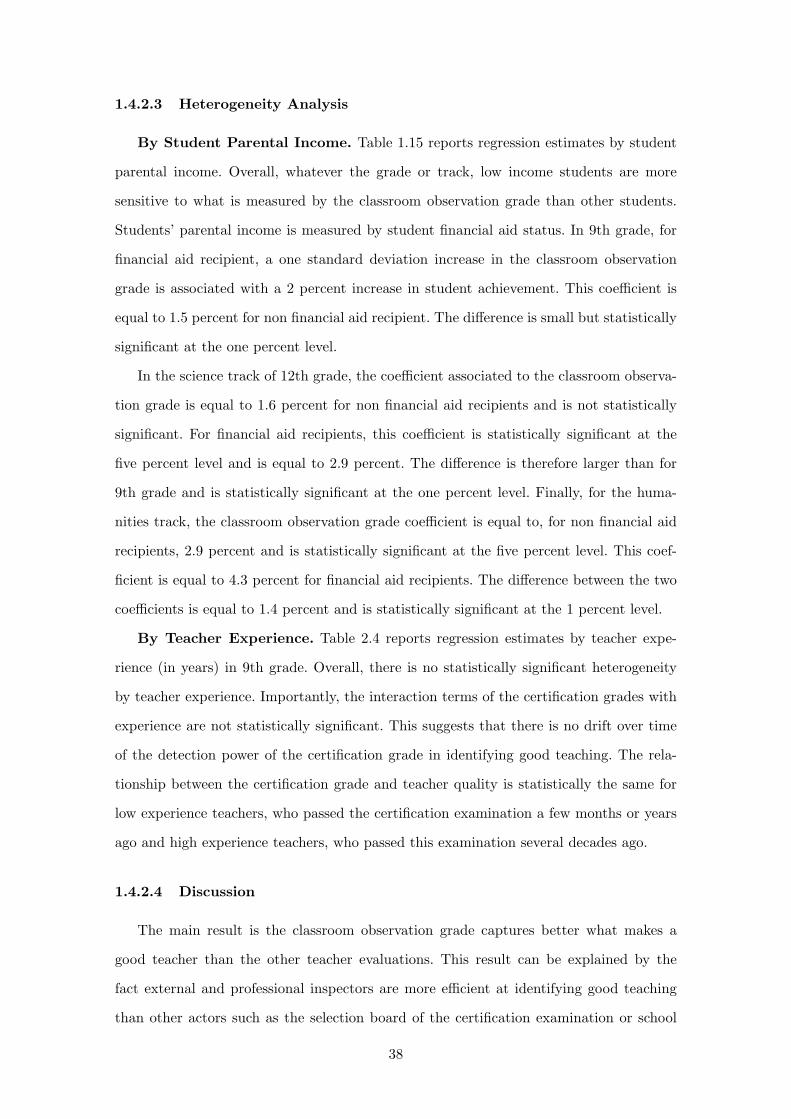
1.4.2.3 Heterogeneity Analysis

By Student Parental Income. Table 1.15 reports regression estimates by student

parental income. Overall, whatever the grade or track, low income students are more

sensitive to what is measured by the classroom observation grade than other students.

Students’ parental income is measured by student financial aid status. In 9th grade, for

financial aid recipient, a one standard deviation increase in the classroom observation

grade is associated with a 2 percent increase in student achievement. This coefficient is

equal to 1.5 percent for non financial aid recipient. The difference is small but statistically

significant at the one percent level.

In the science track of 12th grade, the coefficient associated to the classroom observa-

tion grade is equal to 1.6 percent for non financial aid recipients and is not statistically

significant. For financial aid recipients, this coefficient is statistically significant at the

five percent level and is equal to 2.9 percent. The difference is therefore larger than for

9th grade and is statistically significant at the one percent level. Finally, for the huma-

nities track, the classroom observation grade coefficient is equal to, for non financial aid

recipients, 2.9 percent and is statistically significant at the five percent level. This coef-

ficient is equal to 4.3 percent for financial aid recipients. The difference between the two

coefficients is equal to 1.4 percent and is statistically significant at the 1 percent level.

By Teacher Experience. Table 2.4 reports regression estimates by teacher expe-

rience (in years) in 9th grade. Overall, there is no statistically significant heterogeneity

by teacher experience. Importantly, the interaction terms of the certification grades with

experience are not statistically significant. This suggests that there is no drift over time

of the detection power of the certification grade in identifying good teaching. The rela-

tionship between the certification grade and teacher quality is statistically the same for

low experience teachers, who passed the certification examination a few months or years

ago and high experience teachers, who passed this examination several decades ago.

1.4.2.4 Discussion

The main result is the classroom observation grade captures better what makes a

good teacher than the other teacher evaluations. This result can be explained by the

fact external and professional inspectors are more efficient at identifying good teaching

than other actors such as the selection board of the certification examination or school

38

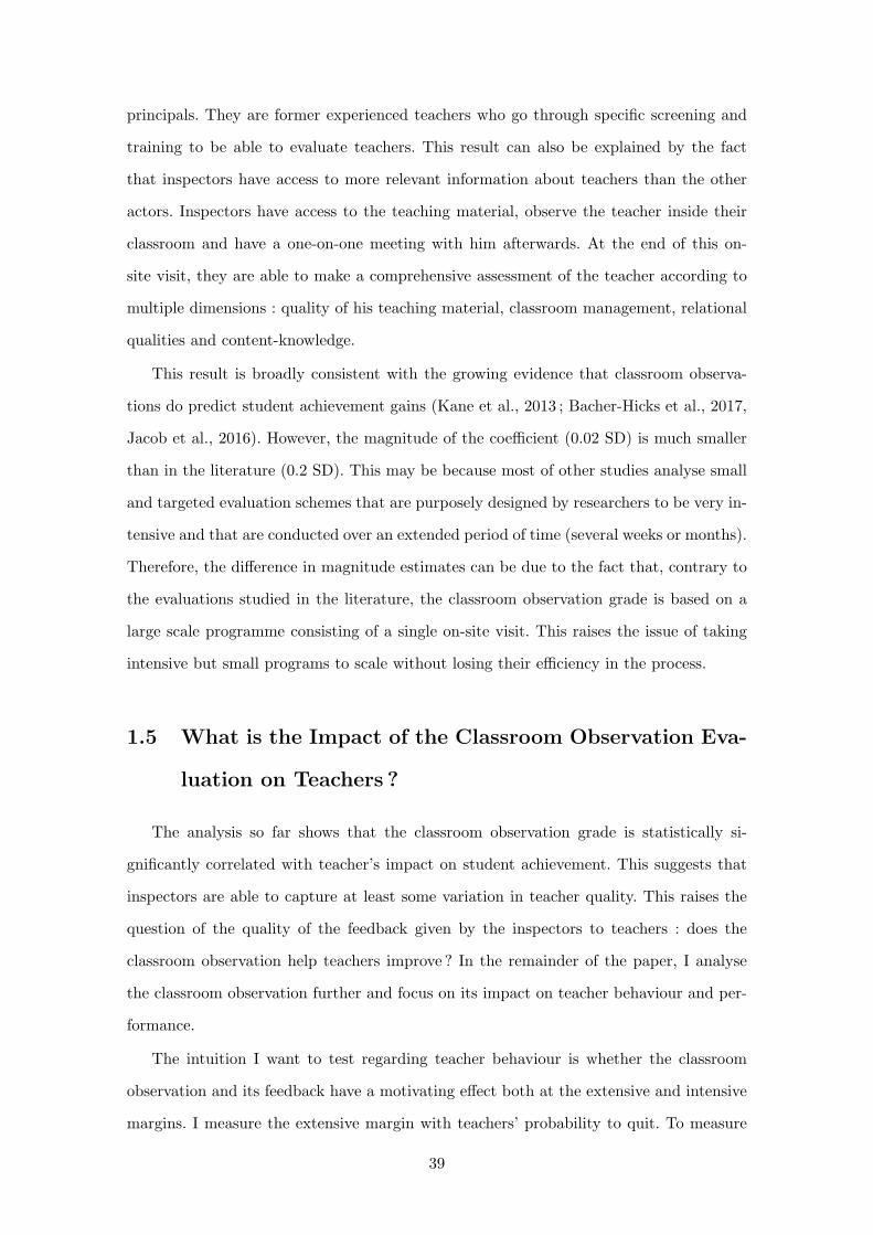
principals. They are former experienced teachers who go through specific screening and

training to be able to evaluate teachers. This result can also be explained by the fact

that inspectors have access to more relevant information about teachers than the other

actors. Inspectors have access to the teaching material, observe the teacher inside their

classroom and have a one-on-one meeting with him afterwards. At the end of this on-

site visit, they are able to make a comprehensive assessment of the teacher according to

multiple dimensions : quality of his teaching material, classroom management, relational

qualities and content-knowledge.

This result is broadly consistent with the growing evidence that classroom observa-

tions do predict student achievement gains (Kane et al., 2013 ; Bacher-Hicks et al., 2017,

Jacob et al., 2016). However, the magnitude of the coefficient (0.02 SD) is much smaller

than in the literature (0.2 SD). This may be because most of other studies analyse small

and targeted evaluation schemes that are purposely designed by researchers to be very in-

tensive and that are conducted over an extended period of time (several weeks or months).

Therefore, the difference in magnitude estimates can be due to the fact that, contrary to

the evaluations studied in the literature, the classroom observation grade is based on a

large scale programme consisting of a single on-site visit. This raises the issue of taking

intensive but small programs to scale without losing their efficiency in the process.

1.5 What is the Impact of the Classroom Observation Eva-

luation on Teachers ?

The analysis so far shows that the classroom observation grade is statistically si-

gnificantly correlated with teacher’s impact on student achievement. This suggests that

inspectors are able to capture at least some variation in teacher quality. This raises the

question of the quality of the feedback given by the inspectors to teachers : does the

classroom observation help teachers improve ? In the remainder of the paper, I analyse

the classroom observation further and focus on its impact on teacher behaviour and per-

formance.

The intuition I want to test regarding teacher behaviour is whether the classroom

observation and its feedback have a motivating effect both at the extensive and intensive

margins. I measure the extensive margin with teachers’ probability to quit. To measure

39

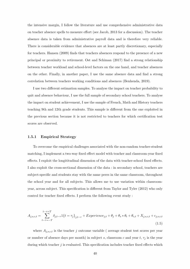
the intensive margin, I follow the literature and use comprehensive administrative data

on teacher absence spells to measure effort (see Jacob, 2013 for a discussion). The teacher

absence data is taken from administrative payroll data and is therefore very reliable.

There is considerable evidence that absences are at least partly discretionary, especially

for teachers. Hansen (2009) finds that teachers absences respond to the presence of a new

principal or proximity to retirement. Ost and Schiman (2017) find a strong relationship

between teacher workload and school-level factors on the one hand, and teacher absences

on the other. Finally, in another paper, I use the same absence data and find a strong

correlation between teachers working conditions and absences (Benhenda, 2019).

I use two different estimation samples. To analyse the impact on teacher probability to

quit and absence behaviour, I use the full sample of secondary school teachers. To analyse

the impact on student achievement, I use the sample of French, Math and History teachers

teaching 9th and 12th grade students. This sample is different from the one exploited in

the previous section because it is not restricted to teachers for which certification test

scores are observed.

1.5.1 Empirical Strategy

To overcome the empirical challenges associated with the non-random teacher-student

matching, I implement a two-way fixed effect model with teacher and classroom-year fixed

effects. I exploit the longititudinal dimension of the data with teacher-school fixed effects.

I also exploit the cross-sectional dimension of the data : in secondary school, teachers are

subject-specific and students stay with the same peers in the same classroom, throughout

the school year and for all subjects. This allows me to use variation within classroom-

year, across subject. This specification is different from Taylor and Tyler (2012) who only

control for teacher fixed effects. I perform the following event study :

Aj,s,c,t =t−τ=T∑

t−τ=−T

δj,t−τ1{t = τj}j,t−τ+Experiencej,t + θj + θs ∗ θt + θc,t +Xj,s,c,t + ǫj,s,c,t

(1.5)

where Aj,s,c,t is the teacher j outcome variable ( average student test scores per year

or number of absence days per month) in subject s, classroom c and year t, τj is the year

during which teacher j is evaluated. This specification includes teacher fixed effects which

40

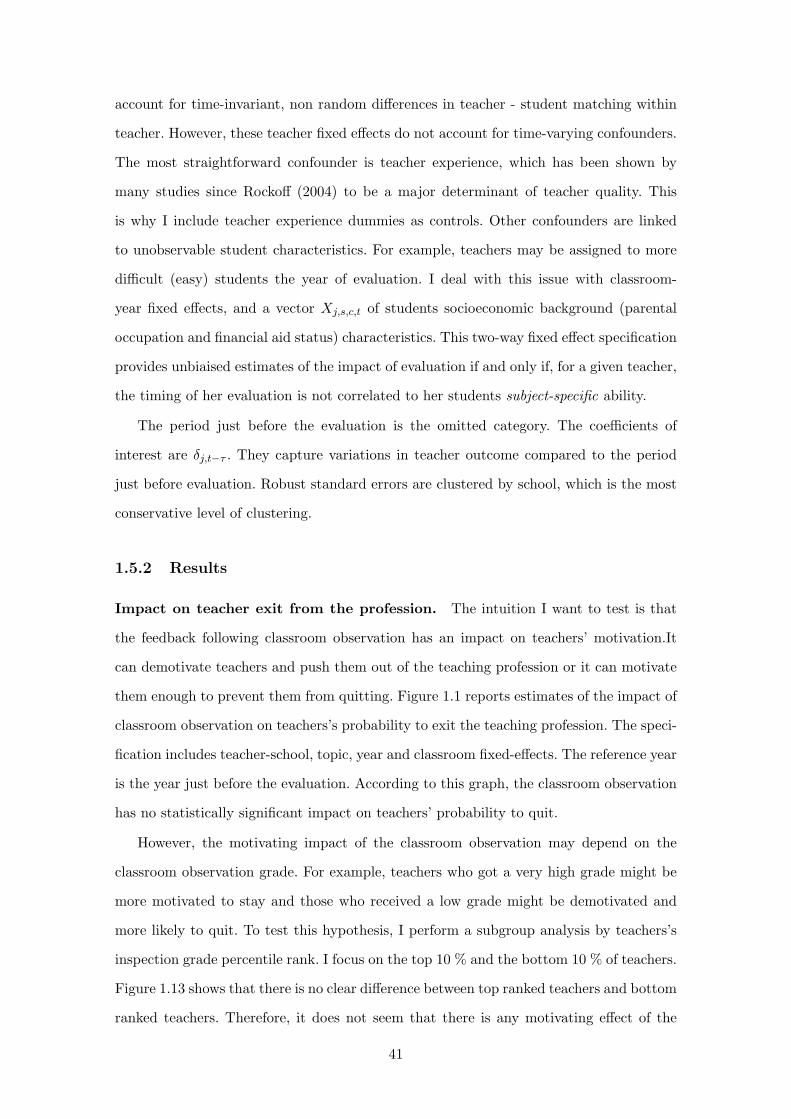
account for time-invariant, non random differences in teacher - student matching within

teacher. However, these teacher fixed effects do not account for time-varying confounders.

The most straightforward confounder is teacher experience, which has been shown by

many studies since Rockoff (2004) to be a major determinant of teacher quality. This

is why I include teacher experience dummies as controls. Other confounders are linked

to unobservable student characteristics. For example, teachers may be assigned to more

difficult (easy) students the year of evaluation. I deal with this issue with classroom-

year fixed effects, and a vector Xj,s,c,t of students socioeconomic background (parental

occupation and financial aid status) characteristics. This two-way fixed effect specification

provides unbiaised estimates of the impact of evaluation if and only if, for a given teacher,

the timing of her evaluation is not correlated to her students subject-specific ability.

The period just before the evaluation is the omitted category. The coefficients of

interest are δj,t−τ . They capture variations in teacher outcome compared to the period

just before evaluation. Robust standard errors are clustered by school, which is the most

conservative level of clustering.

1.5.2 Results

Impact on teacher exit from the profession. The intuition I want to test is that

the feedback following classroom observation has an impact on teachers’ motivation.It

can demotivate teachers and push them out of the teaching profession or it can motivate

them enough to prevent them from quitting. Figure 1.1 reports estimates of the impact of

classroom observation on teachers’s probability to exit the teaching profession. The speci-

fication includes teacher-school, topic, year and classroom fixed-effects. The reference year

is the year just before the evaluation. According to this graph, the classroom observation

has no statistically significant impact on teachers’ probability to quit.

However, the motivating impact of the classroom observation may depend on the

classroom observation grade. For example, teachers who got a very high grade might be

more motivated to stay and those who received a low grade might be demotivated and

more likely to quit. To test this hypothesis, I perform a subgroup analysis by teachers’s

inspection grade percentile rank. I focus on the top 10 % and the bottom 10 % of teachers.

Figure 1.13 shows that there is no clear difference between top ranked teachers and bottom

ranked teachers. Therefore, it does not seem that there is any motivating effect of the

41

classroom observation impacting the probability to quit, even when focusing on top or

bottom ranked teachers.

Impact on teacher absence. The classroom observation does not seem to have an

effect on motivation significant enough to impact teachers’ probability to quit. While it

does not have an impact on the extensive margin, it might impact the intensive margin and

how much effort teachers put into their job. Figure 1.2 shows the classroom observation

has a negative impact on the number of days of teacher absence the year of the evaluation.

Compared to the year just before, teachers are around 0.6 days less absent the year of the

evaluation. This negative impact does not last though and absences are back to their pre-

evaluation levels the year after the evaluation. Note that this result cannot be interpreted

as selection (teachers assigned to better behaved students the year of the evaluation)

because this effect is controlled for in the specification through the classroom-year fixed

effects. This effect can be interpreted as suggesting that the classroom observation has a

motivating effect on teachers, through possibly the feedback it provides. It can also be

interpreted as an incentive effect : teachers have incentives to be less absent in the months

leading to the inspection because the inspector has access to his absence record.

I also investigate whether the motivating effect of the classroom observation varies

teachers’ classroom observation grade. Figure 1.14 shows that there is no clear difference

between top ranked teachers and bottom ranked teachers. Therefore, the classroom ob-

servation does have an statistically significant impact on the number of days of absence,

even when focusing on top or bottom ranked teachers.

Finally, to better understand the mechanisms underpinning this result, I investigate

whether, during the year of inspection, the impact on teacher absence is concentrated in

the months leading to the inspection or in the subsequent months. If the negative impact

on teacher absence is concentrated in the months leading to the inspection, that would

suggest that, in the short run, teacher classroom observation triggers a behavioral response

from teachers by decreasing their effort in the month following the evaluation, as they

know for a fact that they will not be evaluated again during this period. Figure 1.3 reports

estimates of the impact of the classroom observation on the number of teacher absence

days. The specification includes teacher-school, topic, year and month fixed effects. The

reference month is the month just before the evaluation. I observe that teacher are less

42

absent in the months preceding the evaluation than in the months following it. Compared

to the month just before the evaluation, the number of absence days in the months

following the evaluation increases by 0.35-0.5 days.

Thus, overall, this graph suggests that classroom observation triggers a behavioral

response from teachers by temporarily increasing their effort in the month leading to the

evaluation.

Impact on student test scores. Overall, results so far shows that classroom ob-

servation has very limited to no impact on teacher observable behaviour in subsequent

years. While it does not impact observable teacher behaviour, it can still impact teacher

quality if the feedback from inspectors actually helps teachers to improve. Figure 1.4

shows that the classroom observation has no statistically significant impact on student

achievement gains. This suggests that the classroom observation fails to reach one of its

objectives, which is to provide feedback that help teachers improve. However, the impact

of feedback may depend on teacher experience : inexperienced may benefit more from

this feedback than experienced teachers. To test this hypothesis, I perform a subgroup

analysis distinguishing teachers with less than five years of experience from others. The

choice of this five year cutoff is motivated by evidence from the literature showing that

most of the impact of teacher experience on teacher quality is concentrated in the first

five years of teaching (Rockoff, 2004). Figure 1.15 shows that there is no clear difference

between inexperienced teachers and more experienced ones.

1.6 Conclusion

This paper aims at answering the two following questions : how efficient are teacher

evaluations in identifiying good teachers ? Do teacher evaluations have an impact on

subsequent teacher performance ?

In order to answer these questions, I exploit a rich French administrative dataset to

analyse a set of systematic screening and on the job evaluation schemes. I find that the

classroom observation grade is the only evaluation grade significantly related to teacher

performance. I then investigate whether the classroom observation has an impact on

teacher performance and behaviour during the year of evaluation and in subsequent years.

An event study shows that the classroom observation has no statistically significant impact

43

on teacher probability to quit nor on student achievement. I also find that teachers are

slightly less absent during the year of the evaluation, but this effect does not last in this

subsequent years.

Discussion. These results diverge from Taylor and Tyler (2012) who find that teachers

are more productive during the school year when they are being evaluated, and even more

productive in the years after evaluation. In both settings, the evaluations studied have

two dimensions : accountability (they aim at measuring effective teaching) and human

capital formation (personal feedback for teachers). However, both accountability and hu-

man capital formation are much more intensive and thorough in the Cincinnati Teacher

Evaluation scheme analysed by Taylor and Tyler (2012). In the Cincinnati Teacher Eva-

luation, around a hundred of teachers were observed in the classroom and scored four

consecutive times in the school year. Teachers can be fired depending on their evaluation

scores. In my setting, the evaluations are very low stakes : they can only marginally impact

teacher wage progression. Teachers receive thorough feedback, in person and in writing

but it is based on a single observation rather than four. Thus, the difference with Taylor

and Tyler (2012) may stem from two factors. First, it may be because the evaluation is

very low stakes and does not provide strong enough incentives for teachers to change their

behaviour significantly enough. Second, it might also be because the feedback is too noisy

to significantly help teachers improve their teaching practices.

An important point to consider is that Taylor and Tyler (2012) analyse a small and

intensive program, targeted on a few hundreds teachers whereas I study a nationwide pro-

gram designed to manage the whole population of secondary teachers in France (hundred

of thousands of teachers). This is really important for public policy because it highlights

the challenges of taking efficient but small programs to scale (Steinberg and Donaldson,

2016 ; Kraft et al., 2018).

1.7 References

Aaronson, D., Barrow, L., & Sander, W. (2007). Teachers and Student Achie-

vement in the Chicago Public High schools. Journal of Labor Economics, 25(1), 95-135.

Attali, A., & Bressoux, P. (2002). L’evaluation des pratiques educatives dans les

premier et second degres. Rapport pour le Haut conseil de l’evaluation de l’ecole.

44

Bacher-Hicks A., Chin M., Kane T., Staiger D. (2017). An Evaluation of Bias in

Three Measures of Teacher Quality : Value-Added, Classroom Observations, and Student

Surveys, NBER Working Paper.

Benhenda, A. (2019). Absence, Substitutability and Productivity : Evidence from

Teachers, Working Paper.

Boyd, D., Grossman P., Lankford H., Loeb S., & Wyckoff J. (2006). How

Changes in Entry Requirements Alter the Teacher Workforce and Affect Student Achie-

vement. Education Finance and Policy, 1 (2), 176–216.

Bressoux, P. (2008). L’evaluation des enseignants : recommandations pour une

reforme de l’inspection en France. In J. Weiss (Ed.), Quelle evaluation des enseignants

au service de l’ecole ? (pp. 19-28).

Chetty, R., Friedman, J. N., & Rockoff, J. E. (2014). Measuring the Impact

of Teachers I : Evaluating Bias in Teacher Value-Added Estimates. American Economic

Review.

Clotfelter, C. T., Ladd, H. F., & Vigdor, J. L. (2010). Teacher Credentials

and Student Achievement in High School : A Cross-Subject Analysis with Student Fixed

Effects. Journal of Human Resources, 45(3), 655-681.

Dee, T.S. and Wyckoff, J., 2015. Incentives, selection, and teacher performance :

Evidence from IMPACT. Journal of Policy Analysis and Management, 34(2), pp.267-297.

DEPP (2011), Les concours de recrutement de personnels enseignants du second degre

dans l’enseignement public et prive, Note d’information n°11-24, ministere de l’Education

nationale, Direction de l’evaluation, de la prospective et de la performance.

DEPP (2014), Geographie de l’ecole, ministere de l’Education nationale, Direction de

l’evaluation, de la prospective et la performance.

Goldhaber D., Grout C., Huntington-Klein N. (2017). Screen twice, Cut Once :

Assessing the Predictive Validity of Teacher Selection Tools, Educ. Finance Policy, 12 (2),

pp. 197-223

Grosperrin J. (2011), Rapport d’information sur la formation initiale et les mo-

dalites de recrutement des enseignants, Assemblee nationale.

Hansen, M. (2009). How Career Concerns Influence Public Workers’ Effort : Evidence

from the Teacher Labor Market. Working Paper 40. National Center for Analysis of

Longitudinal Data in Education Research.

45

Hanushek, E. A., Kain, J. F., O’Brien, D. M., & Rivkin, S. G. (2005). The

Market for Teacher Quality (No. w11154). National Bureau of Economic Research.

Herrmann, M. A., & Rockoff, J. E. (2012). Worker Absence and Productivity :

Evidence from Teaching, Journal of Labor Economics, 30(4), 749-782.

IGEN (2013a), Les difficultes de recrutement d’enseignants dans certaines disciplines,

rapport au ministre de l’Education nationale, Inspection generale de l’Education natio-

nale.

IGEN (2013b), L’evaluation des enseignants, rapport au ministre de l’Education na-

tionale, Inspection generale de l’Education nationale.

Isore, M. (2009), Teacher Evaluation : Current Practices in OECD Countries and a

Literature Review, OECD Education Working Papers, No. 23, OECD Publishing.

Jackson, C. K. (2014). Teacher Quality at the High-School Level : The Importance

of Accounting for Tracks. Journal of Labor Economics, Vol. 32, No. 4

Jackson, C. K., Rockoff, J. E., & Staiger, D. O. (2014). Teacher Effects and

Teacher-Related Policies. Annual Review of Economics.

Jacob, B. A., & Lefgren, L. (2005). Principals as Agents : Subjective Performance

Measurement in Education (No. w11463). National Bureau of Economic Research.

Jacob, B. A., & Lefgren, L. (2008). Can Principals Identify Effective Teachers ?

Evidence on Subjective Performance Evaluation in Education. Journal of Labor Econo-

mics, 26(1), 101-136.

Jacob, B. A. (2013). The Effect of Employment Protection on Teacher Effort. Journal

of Labor Economics, 31(4), 727-761.

Jacob B., Rockoff J., Taylor E., Lindy B., & Rosen R. (2016). Teacher Appli-

cant Hiring and Teacher Performance : Evidence from DC Public Schools, NBER Working

Paper No. 22054

Kane, T. J., & Staiger, D. O. (2008). Estimating Teacher Impacts on Student

Achievement : An experimental Evaluation (No. w14607). National Bureau of Economic

Research.

Kane, T. J., Rockoff J.E., and Staiger D. (2008). What Does Certification Tell

Us About Teacher Effectiveness ? Evidence from New York City. Economics of Education

Review, 2008, 27 (6),615–631.

Kane, T. J., Taylor, E. S., Tyler, J. H., & Wooten, A. L. (2011). Identi-

46

fying Effective Classroom Practices using Student Achievement Data. Journal of Human

Resources, 46(3), 587-613.

Koedel, C. (2009). An Empirical Analysis of Teacher Spillover Effects in Secondary

School. Economics of Education Review, 28(6), 682-692.

Koedel, C., Mihaly, K., and Rockoff, J. E. (2015). Value-Added Modeling : A

Review. Economics of Education Review, 47, 180-195.

Kramarz, F., Machin, S. & Ouazad, A. (2014). Using Compulsory Mobility to

Identify School Quality and Peer Effects. Oxford Bulletin of Economics and Statistics,

doi : 10.1111/obes.12076.

Kraft, M. A., Brunner, E. J., Dougherty, S. M., Schwegman, D. J. (2018).

Teacher Evaluation Reforms and the Supply and Quality of New Teachers.

Lavy, V. (2010). Do Differences in School’s Instruction Time Explain Internatio-

nal Achievement Gaps in Math, Science, and Reading ? : Evidence from Developed and

Developing Countries. National Bureau of Economic Research.

Loyalka, P., Popova, A., Li, G., Shi, Z. (2019) Does Teacher Training Actually

Work ? Evidence from a Large-Scale Randomized Evaluation of a National Teacher Trai-

ning Program. American Economic Journal : Applied Economics.

Ost, B., & Schiman, J. C. (2017). Workload and Teacher Absence. Economics of

Education Review, 57, 20-30.

Prost, C. (2013). Teacher Mobility : Can Financial Incentives Help Disadvantaged

Schools to Retain their Teachers ?. Annales d’Economie et de Statistique.

Rivkin, S. G., Hanushek, E. A., & Kain, J. F. (2005). Teachers, Schools, and

Academic Achievement. Econometrica, 73(2), 417-458.

Rockoff, J. E. (2004). The Impact of Individual Teachers on Student Achievement :

Evidence from Panel Data. American Economic Review, 247-252.

Staiger D., and Rockoff J. (2010). Searching for Effective Teachers with Imperfect

Information. Journal of Economic Perspectives, 24(3) : 97-118.

Suchaut, B. (2012, February). L’evaluation des enseignants : contexte, analyse et

perspectives d’evolution. In Conference sur l’evaluation, Grenoble (France).

Steinberg, M. P., & Donaldson, M. L. (2016). The New Educational Accoun-

tability : Understanding the Landscape of Teacher Evaluation in the Post-NCLB Era.

Education Finance and Policy, 11(3), 340-359.

47

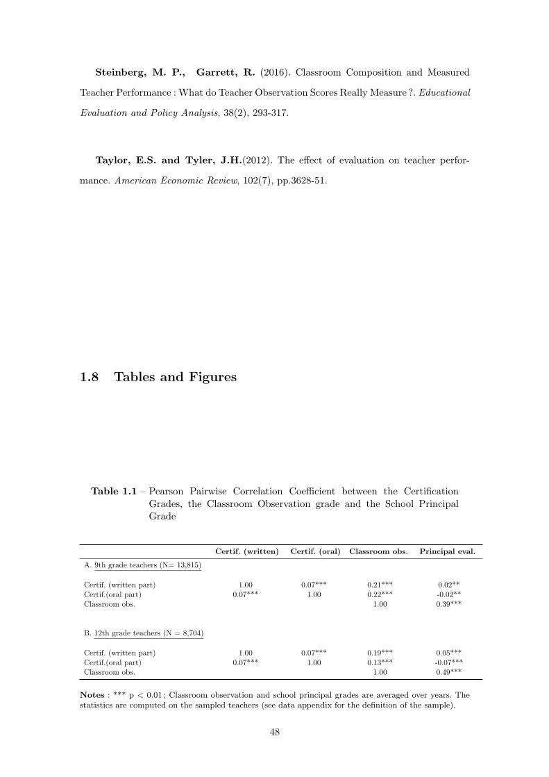
Steinberg, M. P., Garrett, R. (2016). Classroom Composition and Measured

Teacher Performance : What do Teacher Observation Scores Really Measure ?. Educational

Evaluation and Policy Analysis, 38(2), 293-317.

Taylor, E.S. and Tyler, J.H.(2012). The effect of evaluation on teacher perfor-

mance. American Economic Review, 102(7), pp.3628-51.

1.8 Tables and Figures

Table 1.1 – Pearson Pairwise Correlation Coefficient between the CertificationGrades, the Classroom Observation grade and the School PrincipalGrade

Certif. (written) Certif. (oral) Classroom obs. Principal eval.

A. 9th grade teachers (N= 13,815)

Certif. (written part) 1.00 0.07*** 0.21*** 0.02**Certif.(oral part) 0.07*** 1.00 0.22*** -0.02**Classroom obs. 1.00 0.39***

B. 12th grade teachers (N = 8,704)

Certif. (written part) 1.00 0.07*** 0.19*** 0.05***Certif.(oral part) 0.07*** 1.00 0.13*** -0.07***Classroom obs. 1.00 0.49***

Notes : *** p < 0.01 ; Classroom observation and school principal grades are averaged over years. Thestatistics are computed on the sampled teachers (see data appendix for the definition of the sample).

48

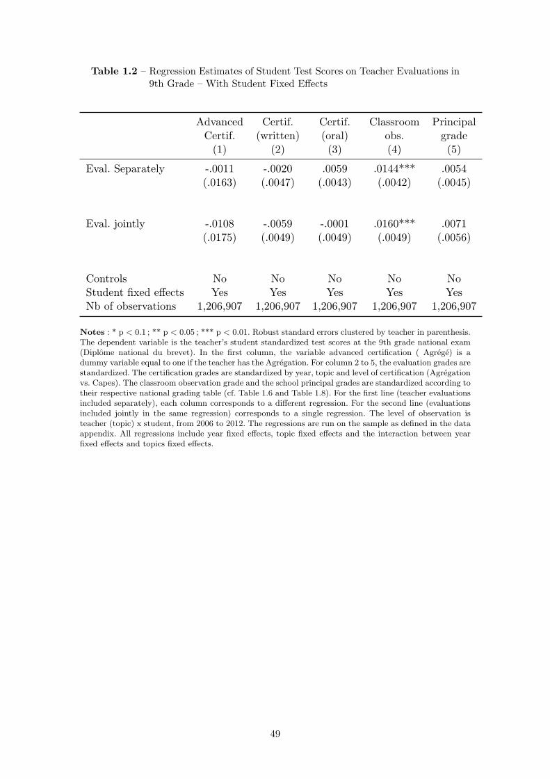
Table 1.2 – Regression Estimates of Student Test Scores on Teacher Evaluations in9th Grade – With Student Fixed Effects

Advanced Certif. Certif. Classroom PrincipalCertif. (written) (oral) obs. grade(1) (2) (3) (4) (5)

Eval. Separately -.0011 -.0020 .0059 .0144*** .0054(.0163) (.0047) (.0043) (.0042) (.0045)

Eval. jointly -.0108 -.0059 -.0001 .0160*** .0071(.0175) (.0049) (.0049) (.0049) (.0056)

Controls No No No No NoStudent fixed effects Yes Yes Yes Yes YesNb of observations 1,206,907 1,206,907 1,206,907 1,206,907 1,206,907

Notes : * p < 0.1 ; ** p < 0.05 ; *** p < 0.01. Robust standard errors clustered by teacher in parenthesis.The dependent variable is the teacher’s student standardized test scores at the 9th grade national exam(Diplome national du brevet). In the first column, the variable advanced certification ( Agrege) is adummy variable equal to one if the teacher has the Agregation. For column 2 to 5, the evaluation grades arestandardized. The certification grades are standardized by year, topic and level of certification (Agregationvs. Capes). The classroom observation grade and the school principal grades are standardized according totheir respective national grading table (cf. Table 1.6 and Table 1.8). For the first line (teacher evaluationsincluded separately), each column corresponds to a different regression. For the second line (evaluationsincluded jointly in the same regression) corresponds to a single regression. The level of observation isteacher (topic) x student, from 2006 to 2012. The regressions are run on the sample as defined in the dataappendix. All regressions include year fixed effects, topic fixed effects and the interaction between yearfixed effects and topics fixed effects.

49

Table 1.3 – Regression Estimates of Student Test Scores on Teacher Evaluations in12th Grade – With Student Fixed Effects

Advanced Certif. Certif. Classroom PrincipalCertif. (written) (oral) Obs. grade(1) (2) (3) (4) (5)

A. Science Track (N =255,128)

Eval. Separately .0300 .0039 .0095 .0230*** .0025(.0174) (.0081) (.0080) (.0089) (.0084)

Eval. jointly .0150 .0024 .0056 .0177* -.0002(.0209) (.0093) ( .0092) ( .0108) (.0094)

B. Humanities Track (N= 149,981)

Eval. Separately -.0089 -.007 .0027 .0202** -.008(.0202) (.0027) (.0099) (.0095) (.006)

Eval. jointly -.0370 -.0129 -.0113 .0311*** -.0064(.0242) (.0108) (.0115) (.0114) (.0103)

Controls No No No No NoStudent fixed effects Yes Yes Yes Yes Yes

Notes : * p < 0.1 ; ** p < 0.05 ; *** p < 0.01. Robust standard errors clustered by teacher in parenthesis.The dependent variable is the teacher’s student standardized test scores at the 12th grade national exam(Baccalaureat). In the first column, Advanced certification( Agrege) is a dummy variable equal to one ifthe teacher has the Agregation. For column 2 to 5, the evaluation grades are standardized. The certificationgrades are standardized by year, topic and level of certification (Agregation vs. Capes). The classroomobservation grade and the school principal grades are standardized according to their respective nationalgrading table (cf. Table 1.6 and Table 1.8). For the first line (teacher evaluations included separately),each column corresponds to a different regression. For the second line (evaluations included jointly in thesame regression) corresponds to a single regression. The level of observation is teacher (topic) x student,from 2006 to 2012. The regressions are run on the sample as defined in the data appendix. All regressionsinclude year fixed effects, topic fixed effects and the interaction between year fixed effects and topics fixedeffects.

50

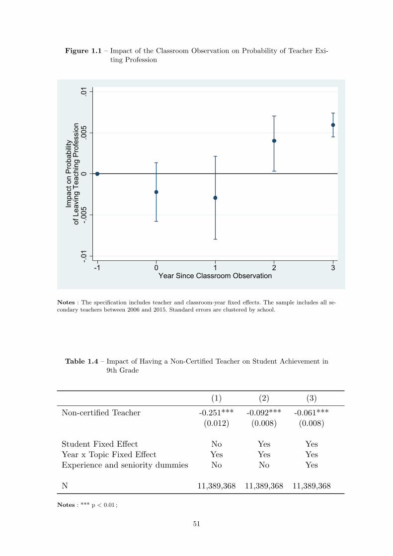
Figure 1.1 – Impact of the Classroom Observation on Probability of Teacher Exi-ting Profession

-.01

-.005

0.0

05.0

1

Impa

ct o

n Pr

obab

ility

of L

eavi

ng T

each

ing

Prof

essi

on

-1 0 1 2 3Year Since Classroom Observation

Notes : The specification includes teacher and classroom-year fixed effects. The sample includes all se-condary teachers between 2006 and 2015. Standard errors are clustered by school.

Table 1.4 – Impact of Having a Non-Certified Teacher on Student Achievement in9th Grade

(1) (2) (3)

Non-certified Teacher -0.251*** -0.092*** -0.061***(0.012) (0.008) (0.008)

Student Fixed Effect No Yes YesYear x Topic Fixed Effect Yes Yes YesExperience and seniority dummies No No Yes

N 11,389,368 11,389,368 11,389,368

Notes : *** p < 0.01 ;

51

Figure 1.2 – Impact of the Classroom Observation on Number of Days of TeacherAbsence in the Subsequent Years

-10

12

3Im

pact

on

Num

ber o

f Day

s of

Tea

cher

Abs

ence

-3 -2 -1 0 1 2Year Since Classroom Observation

Notes : The specification includes teacher and classroom-year fixed effects. The sample includes all se-condary teachers between 2006 and 2015. Standard errors are clustered by school.

52

Figure 1.3 – Impact of the Classroom Observation on Teacher Absence during theYear of Classroom Observation

0.1

.2.3

.4.5

Impa

ct o

n th

e N

umbe

r of T

each

er A

bsen

ce D

ays

(nor

mal

ized

to z

ero

at m

onth

t - 1

)

-5 -4 -3 -2 -1 0 1 2 3 4 5Month Relative to Evaluation

Notes : This figure plots the impact of the classroom observation on the number of teacher absence days(zero included). This corresponds to a single regression. The specification includes teacher-school, topic,year and month fixed effects. The reference month is the month just before the evaluation. The level ofobservation is teacher x classroom x month x year. Robust standard errors are clustered by school.

53

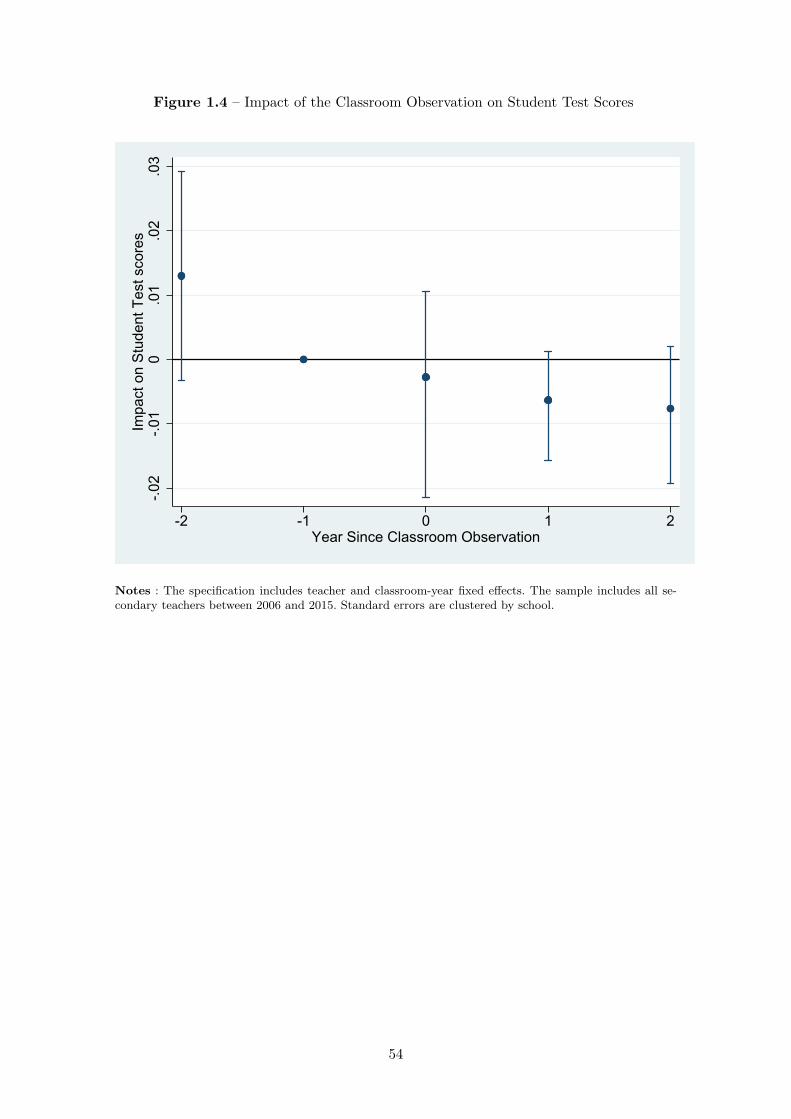
Figure 1.4 – Impact of the Classroom Observation on Student Test Scores

-.02

-.01

0.0

1.0

2.0

3Im

pact

on

Stud

ent T

est s

core

s

-2 -1 0 1 2Year Since Classroom Observation

Notes : The specification includes teacher and classroom-year fixed effects. The sample includes all se-condary teachers between 2006 and 2015. Standard errors are clustered by school.

54

Table 1.5 – Regression Estimates of Certification Grades on Candidates’ IndividualCharacteristics

All PassedDependent variable : Written Grade Oral Grade Written Grade Oral Grade

(1) (2) (3) (4)

Previous occupation (Ref. : Certified teacher)Student 0.182*** 0.234*** -0.515*** -0.075***

(0.007) (0.017) (0.016) (0.020)Contract teacher - 0.141*** 0.100*** -0.458*** -0.017***

(0.008) (0.020) (0.019) (0.023)

Male 0.033*** -0.134*** 0.112*** 0.009***(0.005) (0.009) (0.008) (0.009)

Age -0.016*** -0.018*** -0.008*** -0.009***(0.000) (0.000) (0.000) (0.001)

Degree (Ref. : Bachelor’s degree)Master’s degree -0.141*** -0.050*** 0.115*** -0.043***

(0.007) (0.013) (0.012) (0.014)Grande ecole 0.045 -0.042*** 0.200*** 0.110**

(0.029) (0.054) (0.048) (0.052)

Written exam standardized grade – 0.490*** – 0.089***(0.008) (0.009)

Note : * p < 0.1 ; ** p < 0.05 ; *** p < 0.01. Robust standard errors in parenthesis. This table reportsestimates of regressions of the certification grades (written exam and oral exam) on candidates’ individualcharacteristics. Each column corresponds to a single regression. Columns (1) and (2) reports regressionestimates on all candidates. Columns (3) and (4) reports regression estimates on admitted candidates.The sample is all candidates and all admitted candidates, in all teaching topics, from 2002 to 2012.

1.9 Additional Tables and Figures

Table 1.6 – National Grading Table for the Classroom Observation grade by Cer-tification Level

Basic Certification Advanced CertificationRanking on the wage scale Min. grade Max. grade Min. grade Max. grade

1,2,3,4 32 47 37 485 33 48 39 506 34 49 41 517 35 50 43 548 36 51 45 569 38 53 47 5810 40 55 49 6011 42 57 51 60

Source : French Ministry of Education website (http ://www.education.gouv.fr/cid58632/notations-des-personnels-enseignants.html). This table reports the official national grading table given to inspectors. Forexample, inspectors are instructed to give teachers who have the Capes and are on the fifth rank on thewage scale (echelon) a classroom observation grade comprised between 33 and 48.

55

Table 1.7 – Regression Estimates of the Standardized Classroom Observation gradeon Teacher Characteristics

Dependent variable : Standardized classroom observation grade (1) (2) (3)

Male -0.059*** -0.079*** –(0.020) (0.024)

Experience (in years) 0.034*** 0.032*** 0.064**(0.009) (0.010) (0.028)

Experience2 -0.001 -0.000 -0.002(0.000) (0.000) (0.003)

Subject (Ref. : History)French -0.125*** -0.127*** –

(0.025) (0.028)Math -0.030 -0.018 –

(0.024) (0.027)

Nb of absence spells 0.000 -0.001 -0.003(0.000) (0.003) (0.003)

Nb of days of absence 0.002 0.000 0.002(0.002) (0.000) (0.000)

Adjusted R2 0.006 0.147 0.644School Fixed Effect No Yes NoTeacher Fixed Effect No No Yes

Note : * p < 0.1 ; ** p < 0.05 ; *** p < 0.01. Robust standard errors clustered by teacher in parenthesis.This table reports estimates of regressions of the pedagogical on secondary school teachers (middle and highschool) individual characteristics. Each column corresponds to a single regression. The level of observationis teacher x year. The dependent variable is the standardized (according to the national grading table, cf.Table 1.6).

56

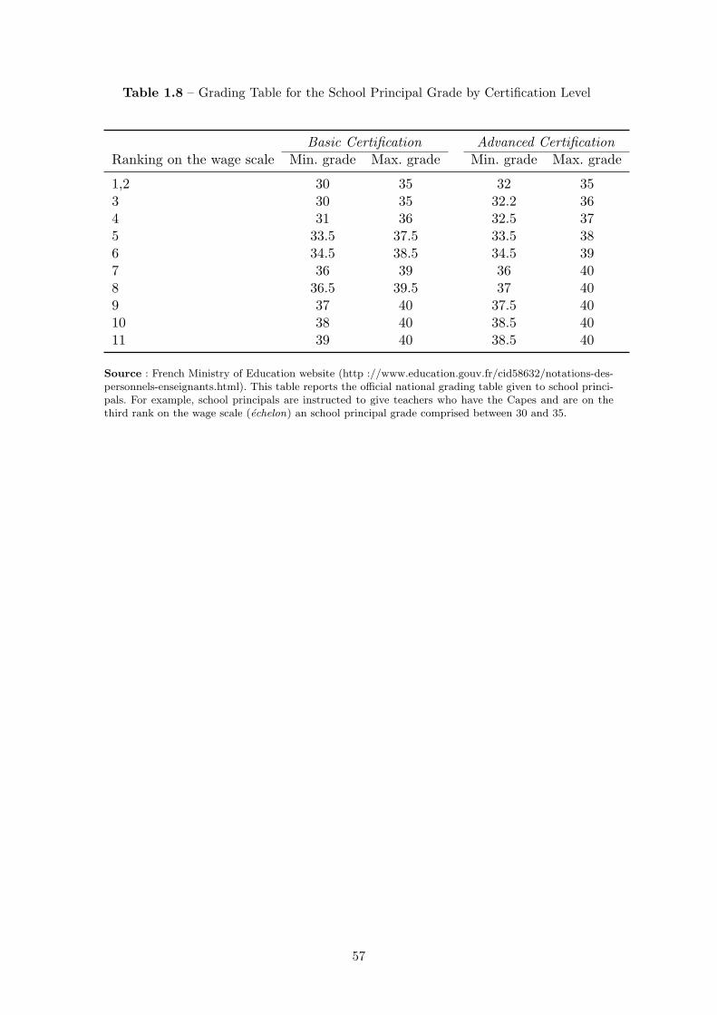
Table 1.8 – Grading Table for the School Principal Grade by Certification Level

Basic Certification Advanced CertificationRanking on the wage scale Min. grade Max. grade Min. grade Max. grade

1,2 30 35 32 353 30 35 32.2 364 31 36 32.5 375 33.5 37.5 33.5 386 34.5 38.5 34.5 397 36 39 36 408 36.5 39.5 37 409 37 40 37.5 4010 38 40 38.5 4011 39 40 38.5 40

Source : French Ministry of Education website (http ://www.education.gouv.fr/cid58632/notations-des-personnels-enseignants.html). This table reports the official national grading table given to school princi-pals. For example, school principals are instructed to give teachers who have the Capes and are on thethird rank on the wage scale (echelon) an school principal grade comprised between 30 and 35.

57

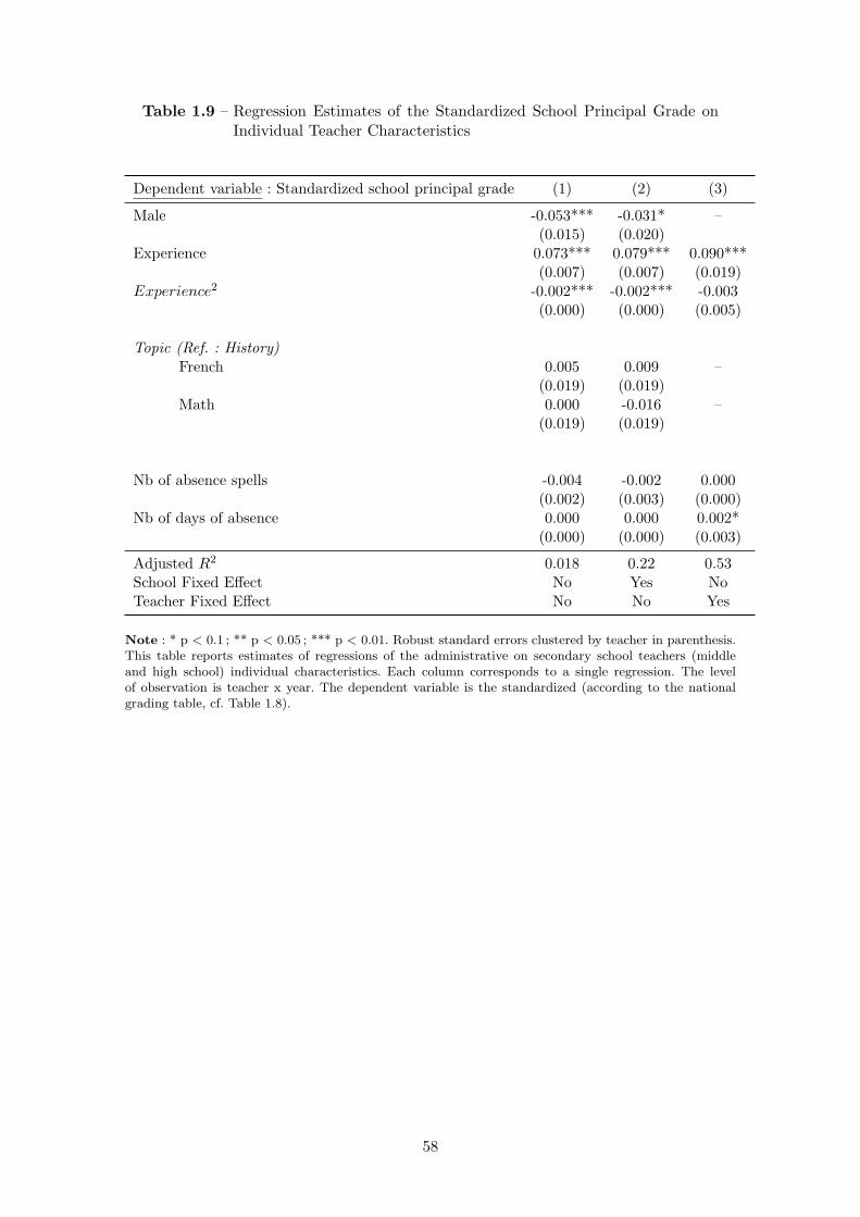
Table 1.9 – Regression Estimates of the Standardized School Principal Grade onIndividual Teacher Characteristics

Dependent variable : Standardized school principal grade (1) (2) (3)

Male -0.053*** -0.031* –(0.015) (0.020)

Experience 0.073*** 0.079*** 0.090***(0.007) (0.007) (0.019)

Experience2 -0.002*** -0.002*** -0.003(0.000) (0.000) (0.005)

Topic (Ref. : History)French 0.005 0.009 –

(0.019) (0.019)Math 0.000 -0.016 –

(0.019) (0.019)

Nb of absence spells -0.004 -0.002 0.000(0.002) (0.003) (0.000)

Nb of days of absence 0.000 0.000 0.002*(0.000) (0.000) (0.003)

Adjusted R2 0.018 0.22 0.53School Fixed Effect No Yes NoTeacher Fixed Effect No No Yes

Note : * p < 0.1 ; ** p < 0.05 ; *** p < 0.01. Robust standard errors clustered by teacher in parenthesis.This table reports estimates of regressions of the administrative on secondary school teachers (middleand high school) individual characteristics. Each column corresponds to a single regression. The levelof observation is teacher x year. The dependent variable is the standardized (according to the nationalgrading table, cf. Table 1.8).

58

Table 1.10 – Average Teacher Characteristics by Grade (All Teachers and SampledTeachers)

All Sample Difference(1) (2) (3) = (1) - (2)

A. Demographics

Female 0.66 0.64 0.02(0.47) (0.48) (0.02)

Age (in years) 41.40 30.20 11.20***(10.10 ) (4.90 ) (0.22)

B. Qualifications

Experience (in years) 15.70 2.90 12.70***(10.2) (1.30) (0.07)

Advanced Certif. 0.06 0.09 -0.03**(0.25) (0.28) (0.01)

Basic Certif. 0.84 0.85 -.01(0.36) (0.35) (0.01)

Other certification status 0.09 0.06 0.03***(0.29) (0.24) (0.01)

C. School

Average school size 471.80 544.28 -72.40***(213.90) (201.90) (8.80)

Teaching in the Parisian suburbs 0.16 0.38 -0.22***(0.37) (0.49) (0.02)

Number of teachers 106,892 22,519

Notes : The t-statistic for the comparison of means (columns 3 and 6 ) is equal to the ratio of the mean ofthe difference to the standard error of the difference. * p < 0.1 ; ** p < 0.05 ; *** p < 0.01. Standard errorsin parenthesis. The statistics are reported for all secondary school teachers (column 1) and for teachers inthe estimation sample(column 2), as defined in the data appendix.

59

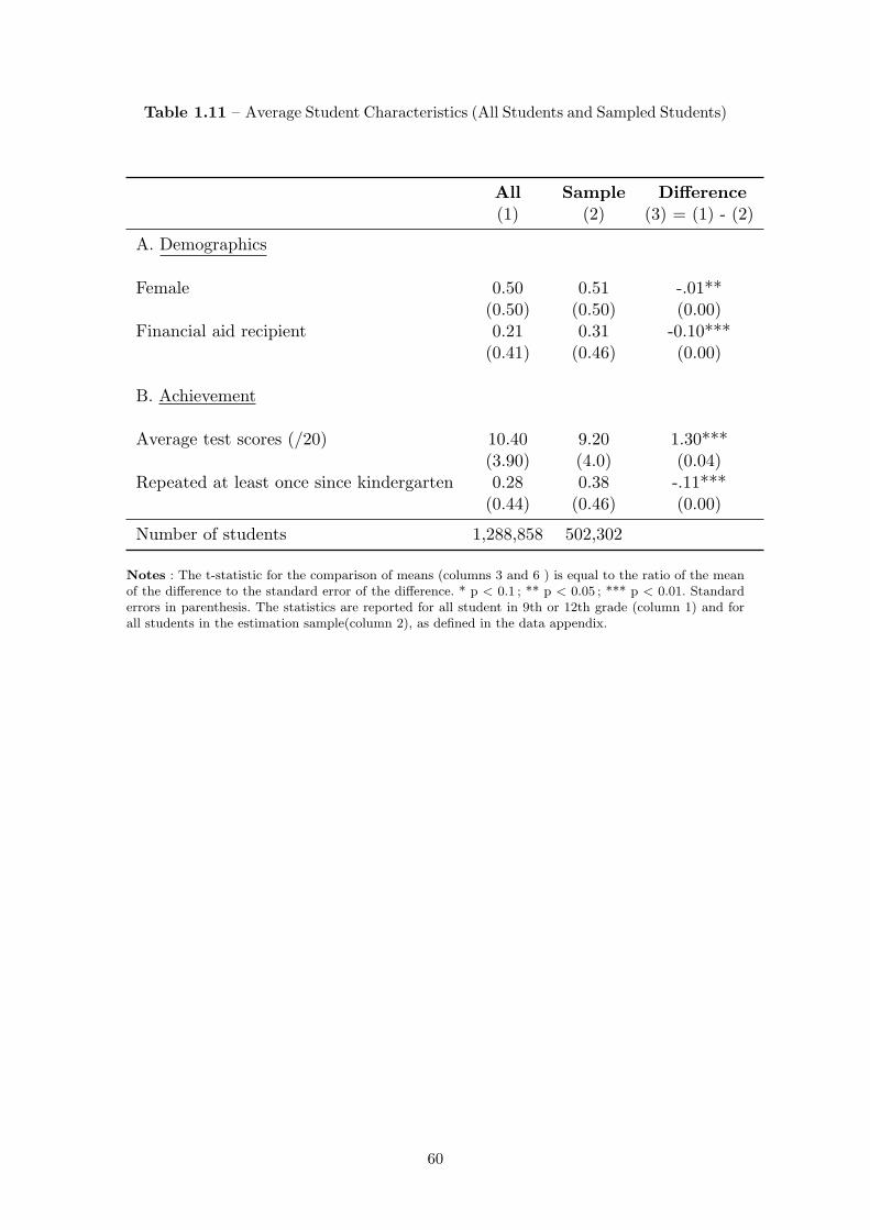
Table 1.11 – Average Student Characteristics (All Students and Sampled Students)

All Sample Difference(1) (2) (3) = (1) - (2)

A. Demographics

Female 0.50 0.51 -.01**(0.50) (0.50) (0.00)

Financial aid recipient 0.21 0.31 -0.10***(0.41) (0.46) (0.00)

B. Achievement

Average test scores (/20) 10.40 9.20 1.30***(3.90) (4.0) (0.04)

Repeated at least once since kindergarten 0.28 0.38 -.11***(0.44) (0.46) (0.00)

Number of students 1,288,858 502,302

Notes : The t-statistic for the comparison of means (columns 3 and 6 ) is equal to the ratio of the meanof the difference to the standard error of the difference. * p < 0.1 ; ** p < 0.05 ; *** p < 0.01. Standarderrors in parenthesis. The statistics are reported for all student in 9th or 12th grade (column 1) and forall students in the estimation sample(column 2), as defined in the data appendix.

60

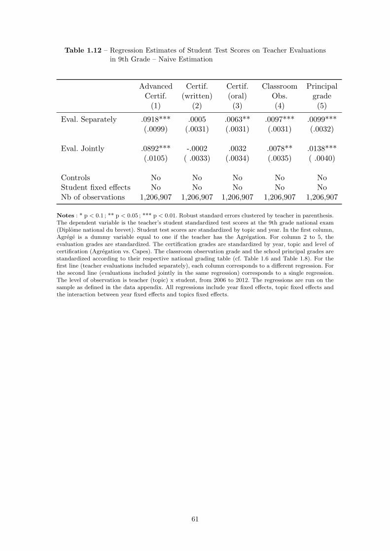
Table 1.12 – Regression Estimates of Student Test Scores on Teacher Evaluationsin 9th Grade – Naive Estimation

Advanced Certif. Certif. Classroom PrincipalCertif. (written) (oral) Obs. grade(1) (2) (3) (4) (5)

Eval. Separately .0918*** .0005 .0063** .0097*** .0099***(.0099) (.0031) (.0031) (.0031) (.0032)

Eval. Jointly .0892*** -.0002 .0032 .0078** .0138***(.0105) ( .0033) (.0034) (.0035) ( .0040)

Controls No No No No NoStudent fixed effects No No No No NoNb of observations 1,206,907 1,206,907 1,206,907 1,206,907 1,206,907

Notes : * p < 0.1 ; ** p < 0.05 ; *** p < 0.01. Robust standard errors clustered by teacher in parenthesis.The dependent variable is the teacher’s student standardized test scores at the 9th grade national exam(Diplome national du brevet). Student test scores are standardized by topic and year. In the first column,Agrege is a dummy variable equal to one if the teacher has the Agregation. For column 2 to 5, theevaluation grades are standardized. The certification grades are standardized by year, topic and level ofcertification (Agregation vs. Capes). The classroom observation grade and the school principal grades arestandardized according to their respective national grading table (cf. Table 1.6 and Table 1.8). For thefirst line (teacher evaluations included separately), each column corresponds to a different regression. Forthe second line (evaluations included jointly in the same regression) corresponds to a single regression.The level of observation is teacher (topic) x student, from 2006 to 2012. The regressions are run on thesample as defined in the data appendix. All regressions include year fixed effects, topic fixed effects andthe interaction between year fixed effects and topics fixed effects.

61

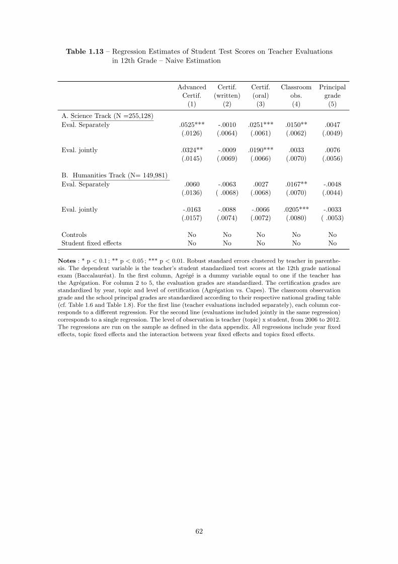
Table 1.13 – Regression Estimates of Student Test Scores on Teacher Evaluationsin 12th Grade – Naive Estimation

Advanced Certif. Certif. Classroom PrincipalCertif. (written) (oral) obs. grade(1) (2) (3) (4) (5)

A. Science Track (N =255,128)

Eval. Separately .0525*** -.0010 .0251*** .0150** .0047(.0126) (.0064) (.0061) (.0062) (.0049)

Eval. jointly .0324** -.0009 .0190*** .0033 .0076(.0145) (.0069) (.0066) (.0070) (.0056)

B. Humanities Track (N= 149,981)

Eval. Separately .0060 -.0063 .0027 .0167** -.0048(.0136) ( .0068) (.0068) (.0070) (.0044)

Eval. jointly -.0163 -.0088 -.0066 .0205*** -.0033(.0157) (.0074) (.0072) (.0080) ( .0053)

Controls No No No No NoStudent fixed effects No No No No No

Notes : * p < 0.1 ; ** p < 0.05 ; *** p < 0.01. Robust standard errors clustered by teacher in parenthe-sis. The dependent variable is the teacher’s student standardized test scores at the 12th grade nationalexam (Baccalaureat). In the first column, Agrege is a dummy variable equal to one if the teacher hasthe Agregation. For column 2 to 5, the evaluation grades are standardized. The certification grades arestandardized by year, topic and level of certification (Agregation vs. Capes). The classroom observationgrade and the school principal grades are standardized according to their respective national grading table(cf. Table 1.6 and Table 1.8). For the first line (teacher evaluations included separately), each column cor-responds to a different regression. For the second line (evaluations included jointly in the same regression)corresponds to a single regression. The level of observation is teacher (topic) x student, from 2006 to 2012.The regressions are run on the sample as defined in the data appendix. All regressions include year fixedeffects, topic fixed effects and the interaction between year fixed effects and topics fixed effects.

62

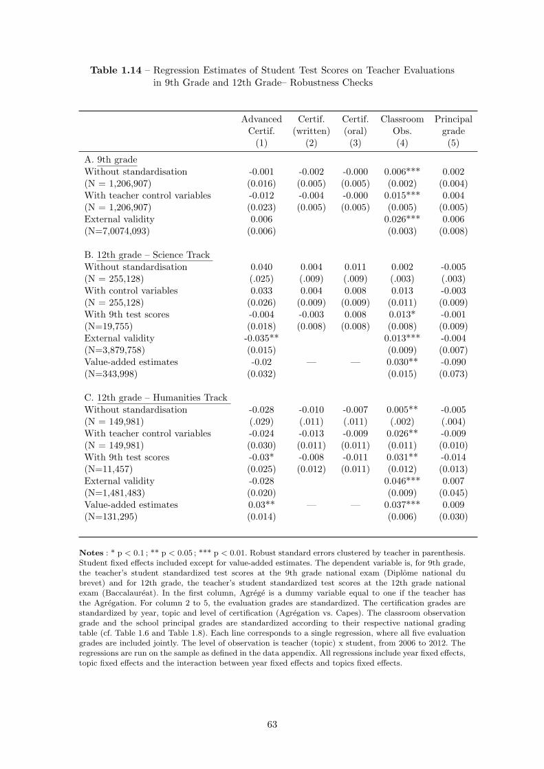
Table 1.14 – Regression Estimates of Student Test Scores on Teacher Evaluationsin 9th Grade and 12th Grade– Robustness Checks

Advanced Certif. Certif. Classroom PrincipalCertif. (written) (oral) Obs. grade(1) (2) (3) (4) (5)

A. 9th grade

Without standardisation -0.001 -0.002 -0.000 0.006*** 0.002(N = 1,206,907) (0.016) (0.005) (0.005) (0.002) (0.004)With teacher control variables -0.012 -0.004 -0.000 0.015*** 0.004(N = 1,206,907) (0.023) (0.005) (0.005) (0.005) (0.005)External validity 0.006 0.026*** 0.006(N=7,0074,093) (0.006) (0.003) (0.008)

B. 12th grade – Science Track

Without standardisation 0.040 0.004 0.011 0.002 -0.005(N = 255,128) (.025) (.009) (.009) (.003) (.003)With control variables 0.033 0.004 0.008 0.013 -0.003(N = 255,128) (0.026) (0.009) (0.009) (0.011) (0.009)With 9th test scores -0.004 -0.003 0.008 0.013* -0.001(N=19,755) (0.018) (0.008) (0.008) (0.008) (0.009)External validity -0.035** 0.013*** -0.004(N=3,879,758) (0.015) (0.009) (0.007)Value-added estimates -0.02 — — 0.030** -0.090(N=343,998) (0.032) (0.015) (0.073)

C. 12th grade – Humanities Track

Without standardisation -0.028 -0.010 -0.007 0.005** -0.005(N = 149,981) (.029) (.011) (.011) (.002) (.004)With teacher control variables -0.024 -0.013 -0.009 0.026** -0.009(N = 149,981) (0.030) (0.011) (0.011) (0.011) (0.010)With 9th test scores -0.03* -0.008 -0.011 0.031** -0.014(N=11,457) (0.025) (0.012) (0.011) (0.012) (0.013)External validity -0.028 0.046*** 0.007(N=1,481,483) (0.020) (0.009) (0.045)Value-added estimates 0.03** — — 0.037*** 0.009(N=131,295) (0.014) (0.006) (0.030)

Notes : * p < 0.1 ; ** p < 0.05 ; *** p < 0.01. Robust standard errors clustered by teacher in parenthesis.Student fixed effects included except for value-added estimates. The dependent variable is, for 9th grade,the teacher’s student standardized test scores at the 9th grade national exam (Diplome national dubrevet) and for 12th grade, the teacher’s student standardized test scores at the 12th grade nationalexam (Baccalaureat). In the first column, Agrege is a dummy variable equal to one if the teacher hasthe Agregation. For column 2 to 5, the evaluation grades are standardized. The certification grades arestandardized by year, topic and level of certification (Agregation vs. Capes). The classroom observationgrade and the school principal grades are standardized according to their respective national gradingtable (cf. Table 1.6 and Table 1.8). Each line corresponds to a single regression, where all five evaluationgrades are included jointly. The level of observation is teacher (topic) x student, from 2006 to 2012. Theregressions are run on the sample as defined in the data appendix. All regressions include year fixed effects,topic fixed effects and the interaction between year fixed effects and topics fixed effects.

63

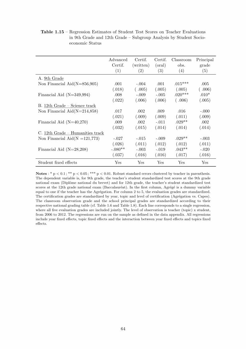
Table 1.15 – Regression Estimates of Student Test Scores on Teacher Evaluationsin 9th Grade and 12th Grade – Subgroup Analysis by Student Socio-economic Status

Advanced Certif. Certif. Classroom PrincipalCertif. (written) (oral) obs. grade(1) (2) (3) (4) (5)

A. 9th GradeNon Financial Aid(N=856,905) .001 -.004 .001 .015*** .005

(.018) ( .005) (.005) (.005) ( .006)Financial Aid (N=349,994) .008 -.009 -.005 .020*** .010*

(.022) (.006) (.006) ( .006) (.005)B. 12th Grade – Science trackNon Financial Aid(N=214,858) .017 .002 .009 .016 -.000

(.021) (.009) (.009) (.011) (.009)Financial Aid (N=40,270) .009 .002 -.011 .029** .002

(.032) (.015) (.014) (.014) (.014)C. 12th Grade – Humanities trackNon Financial Aid(N =121,773) -.027 -.015 -.009 .029** -.003

(.026) (.011) (.012) (.012) (.011)Financial Aid (N=28,208) -.080** -.003 -.019 .043** -.020

(.037) (.016) (.016) (.017) (.016)

Student fixed effects Yes Yes Yes Yes Yes

Notes : * p < 0.1 ; ** p < 0.05 ; *** p < 0.01. Robust standard errors clustered by teacher in parenthesis.The dependent variable is, for 9th grade, the teacher’s student standardized test scores at the 9th gradenational exam (Diplome national du brevet) and for 12th grade, the teacher’s student standardized testscores at the 12th grade national exam (Baccalaureat). In the first column, Agrege is a dummy variableequal to one if the teacher has the Agregation. For column 2 to 5, the evaluation grades are standardized.The certification grades are standardized by year, topic and level of certification (Agregation vs. Capes).The classroom observation grade and the school principal grades are standardized according to theirrespective national grading table (cf. Table 1.6 and Table 1.8). Each line corresponds to a single regression,where all five evaluation grades are included jointly. The level of observation is teacher (topic) x student,from 2006 to 2012. The regressions are run on the sample as defined in the data appendix. All regressionsinclude year fixed effects, topic fixed effects and the interaction between year fixed effects and topics fixedeffects.

64

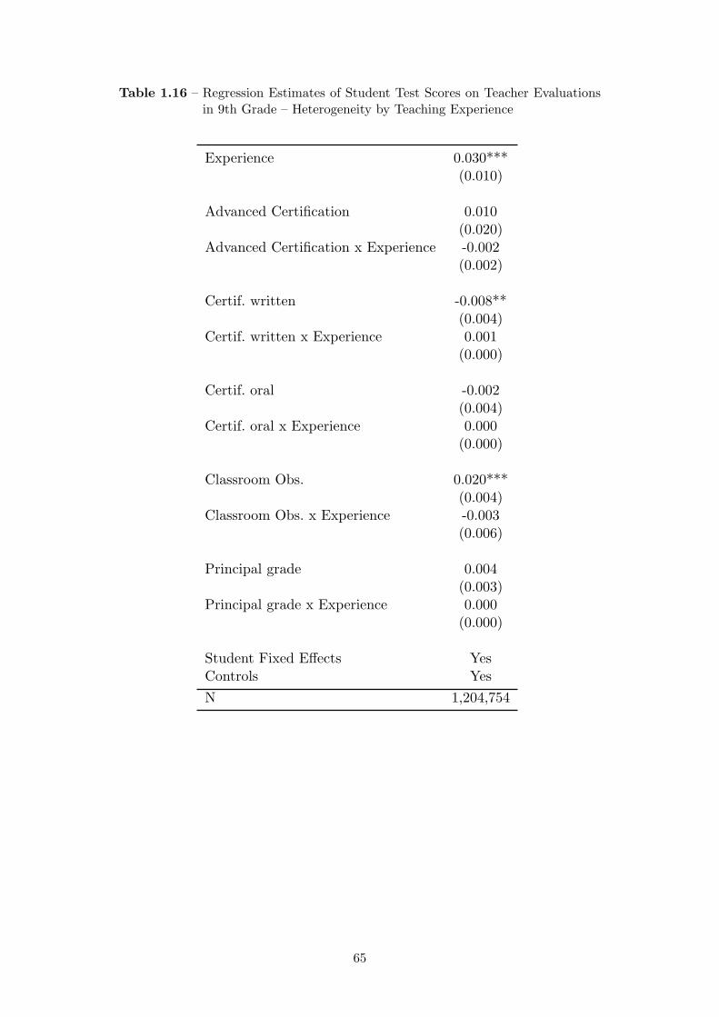
Table 1.16 – Regression Estimates of Student Test Scores on Teacher Evaluationsin 9th Grade – Heterogeneity by Teaching Experience

Experience 0.030***(0.010)

Advanced Certification 0.010(0.020)

Advanced Certification x Experience -0.002(0.002)

Certif. written -0.008**(0.004)

Certif. written x Experience 0.001(0.000)

Certif. oral -0.002(0.004)

Certif. oral x Experience 0.000(0.000)

Classroom Obs. 0.020***(0.004)

Classroom Obs. x Experience -0.003(0.006)

Principal grade 0.004(0.003)

Principal grade x Experience 0.000(0.000)

Student Fixed Effects YesControls Yes

N 1,204,754

65

Figure 1.5 – Kernel Density of the Certification Grades (Written and Oral) for allCandidates and for Passing Candidates

0.0

5.1

.15

.2D

ensi

ty

0 5 10 15 20Grade (/20)

Writ.(All) Oral (All)

Writ.(Pass.) Oral(Pass.)

CAPES

0.0

5.1

.15

.2D

ensi

ty

0 5 10 15 20Grade (/20)

Writ.(All) Oral (All)

Writ. (Pass.) Oral(Pass.)

Agrégation

Notes : This figure plots the kernel density of the written exam grade (blue line) and the oral exam grade(red line) for all candidates (solid line) and for candidates who passed the exam (dotted line). The leftgraph plots the density for the Capes and the right graph plots the density for the Agregation. The sampleincludes all the candidates who are present to the exam (see notes to Figure ??) from 2002 to 2012, inMath, French and History.

66

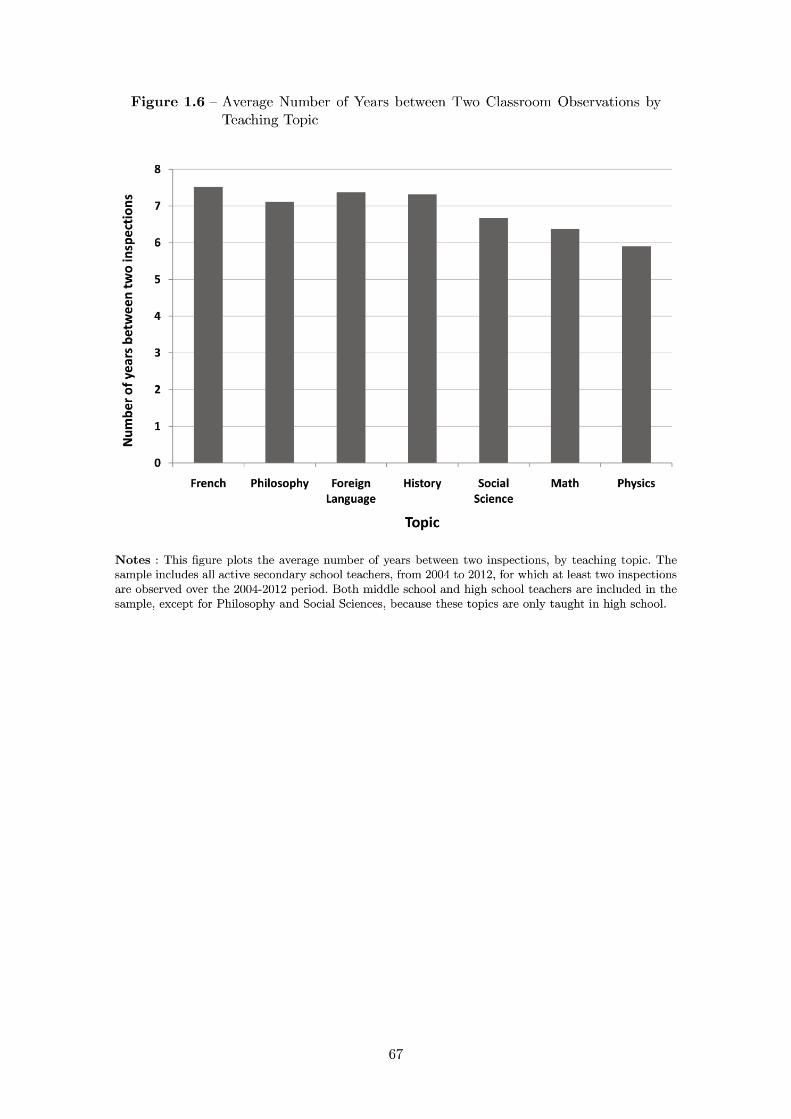
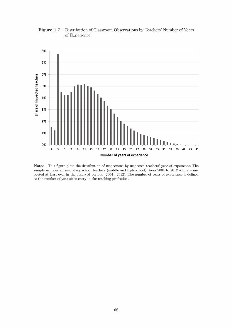
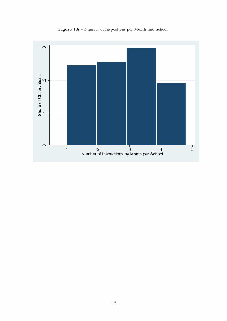
Figure 1.8 – Number of Inspections per Month and School

0.1

.2.3

Shar

e of

Obs

erva

tions

1 2 3 4 5Number of Inspections by Month per School

69

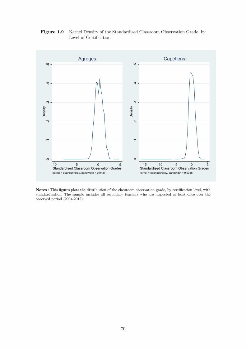
Figure 1.9 – Kernel Density of the Standardised Classroom Observation Grade, byLevel of Certification

0.1

.2.3

.4.5

Den

sity

-10 -5 0 5Standardised Classroom Observation Gradeskernel = epanechnikov, bandwidth = 0.0437

Agreges

0.1

.2.3

.4.5

Den

sity

-15 -10 -5 0 5Standardised Classroom Observation Gradeskernel = epanechnikov, bandwidth = 0.0356

Capetiens

Notes : This figures plots the distribution of the classroom observation grade, by certification level, withstandardisation. The sample includes all secondary teachers who are inspected at least once over theobserved period (2004-2012).

70

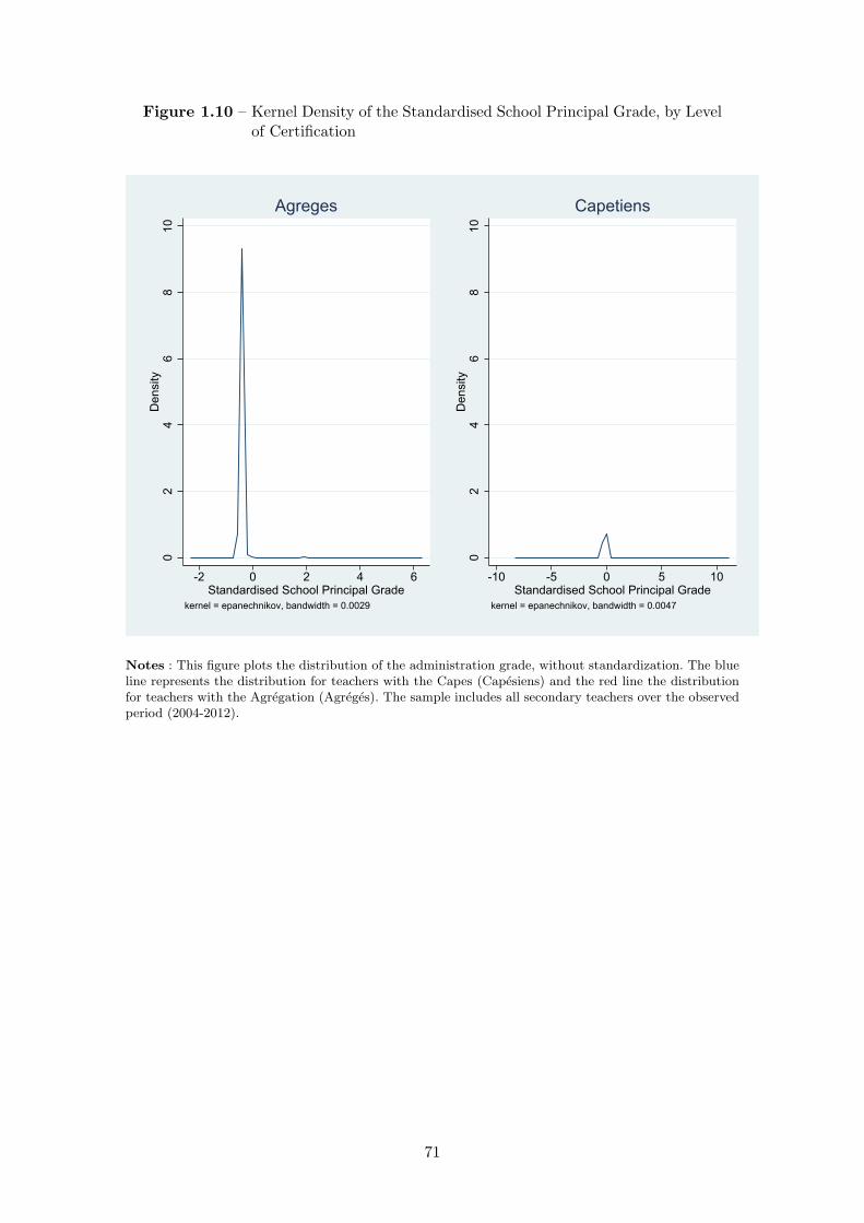
Figure 1.10 – Kernel Density of the Standardised School Principal Grade, by Levelof Certification

02

46

810

Den

sity

-2 0 2 4 6Standardised School Principal Grade

kernel = epanechnikov, bandwidth = 0.0029

Agreges

02

46

810

Den

sity

-10 -5 0 5 10Standardised School Principal Grade

kernel = epanechnikov, bandwidth = 0.0047

Capetiens

Notes : This figure plots the distribution of the administration grade, without standardization. The blueline represents the distribution for teachers with the Capes (Capesiens) and the red line the distributionfor teachers with the Agregation (Agreges). The sample includes all secondary teachers over the observedperiod (2004-2012).

71

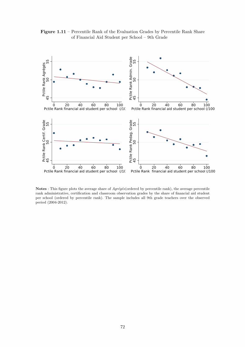
Figure 1.11 – Percentile Rank of the Evaluation Grades by Percentile Rank Shareof Financial Aid Student per School – 9th Grade

45

50

55

Pct

ile R

ank

Agré

gés

0 20 40 60 80 100Pctile Rank financial aid student per school (/100)

45

50

55

Pct

ile R

ank

Adm

in. G

rade

0 20 40 60 80 100Pctile Rank financial aid student per school (/100)

45

50

55

Pct

ile R

ank

Cert

if. G

rade

0 20 40 60 80 100Pctile Rank financial aid student per school (/100)

45

50

55

Pct

ile R

ank

Pedag. G

rade

0 20 40 60 80 100Pctile Rank financial aid student per school (/100)

Notes : This figure plots the average share of Agreges(ordered by percentile rank), the average percentilerank administrative, certification and classroom observation grades by the share of financial aid studentper school (ordered by percentile rank). The sample includes all 9th grade teachers over the observedperiod (2004-2012).

72

Figure 1.12 – Percentile Rank of the Evaluation Grades by Percentile Rank Shareof Financial Aid Student per School – 12th Grade

30

40

50

60

70

Pct

ile R

ank

Agré

gés

0 20 40 60 80 100Pctile Rank financial aid student per school (/100)

30

40

50

60

70

Pct

ile R

ank

Adm

in. G

rade

0 20 40 60 80 100Pctile Rank financial aid student per school (/100)

30

40

50

60

70

Pct

ile R

ank

Cert

if. G

rade

0 20 40 60 80 100Pctile Rank financial aid student per school (/100)

30

40

50

60

70

Pct

ile R

ank

Pedag. G

rade

0 20 40 60 80 100Pctile Rank financial aid student per school (/100)

Notes : This figure plots the average share of Agreges(ordered by percentile rank), the average percentilerank administrative, certification and classroom observation grades by the share of financial aid studentper school (ordered by percentile rank). The sample includes all 12th grade teachers over the observedperiod (2004-2012).

73

Figure 1.13 – Impact of the Classroom Observation on Probability to Quit by Tea-chers’ Performance at the Classroom Observation

-.05

0.0

5.1

Impa

ct o

n Pr

obab

ility

on T

each

er M

obilit

y Ac

ross

Sch

ools

-1 0 1 2Year Since Classroom Observation

Top 10% Classroom Observation Grade Bottom 10 % Classroom Observation Grade

Notes : The specification includes teacher and classroom-year fixed effects. The sample includes all se-condary teachers between 2006 and 2015. Standard errors are clustered by school.

74

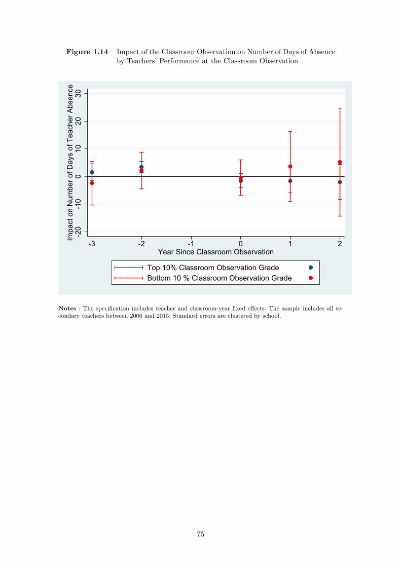
Figure 1.14 – Impact of the Classroom Observation on Number of Days of Absenceby Teachers’ Performance at the Classroom Observation

-20

-10

010

2030

Impa

ct o

n N

umbe

r of D

ays

of T

each

er A

bsen

ce

-3 -2 -1 0 1 2Year Since Classroom Observation

Top 10% Classroom Observation Grade Bottom 10 % Classroom Observation Grade

Notes : The specification includes teacher and classroom-year fixed effects. The sample includes all se-condary teachers between 2006 and 2015. Standard errors are clustered by school.

75

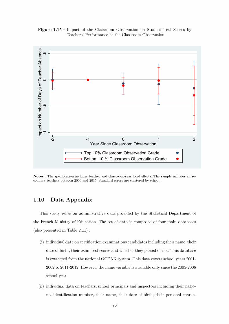
Figure 1.15 – Impact of the Classroom Observation on Student Test Scores byTeachers’ Performance at the Classroom Observation

-1-.5

0.5

Impa

ct o

n N

umbe

r of D

ays

of T

each

er A

bsen

ce

-2 -1 0 1 2Year Since Classroom Observation

Top 10% Classroom Observation Grade Bottom 10 % Classroom Observation Grade

Notes : The specification includes teacher and classroom-year fixed effects. The sample includes all se-condary teachers between 2006 and 2015. Standard errors are clustered by school.

1.10 Data Appendix

This study relies on administrative data provided by the Statistical Department of

the French Ministry of Education. The set of data is composed of four main databases

(also presented in Table 2.11) :

(i) individual data on certification examinations candidates including their name, their

date of birth, their exam test scores and whether they passed or not. This database

is extracted from the national OCEAN system. This data covers school years 2001-

2002 to 2011-2012. However, the name variable is available only since the 2005-2006

school year.

(ii) individual data on teachers, school principals and inspectors including their natio-

nal identification number, their name, their date of birth, their personal charac-

76

teristics. For teachers, the data includes their teaching subject(s), and, crucially,

the identification number of the school and of the class in which they teach. All

this information is mainly available in two databases, called Annuaires and Relais.

These two databases cover school years 2001-2002 to 2014-2015. These two data-

bases are merged with data on certification examinations based on the name, sex

and date of birth variables.

(iii) individual data on students including socio-demographic characteristics such as

gender and financial aid status 7 (bourse sur criteres sociaux ), an encrypted natio-

nal identification number, their grades on the two national and externally grades

examinations taken in the final year of 9th grade (the Diplome national du brevet

– hereafter DNB) and in the final year of 12th grade (Baccalaureat), the identifi-

cation number of their school and of their class. These two latter variables enable

us to match each teacher to her students. All this information is collected at the

regional level (in databases called Bases eleve academique) and gathered in a single

national database by the Statistical department of the Ministry of Education. This

database covers school years 2005-2006 to 2014-2015.

iv individual data on teacher absence spells for 9th grade teachers including the

detailed dates of the absence spells. This datasets is mergeed with the other teacher

data through teacher’s individual identifier.

The construction of the final samples required numerous and sometimes delicate

merges between the different databases. The main merging procedures and their out-

comes are described in detail in the data appendix.

7. The financial aid status is not reliable in the student database commonly used in France (Basecentrale scolarite). This is because the Base centrale scolarite is a beginning of the school year photography.At the beginning of the school year, the information on students’ financial status is still incomplete. Thedatabase we are using here is an end of the school year of photography. At the end of the school year, theinformation on students’ financial status is complete. Therefore, the financial aid status variable we areusing is reliable.

77

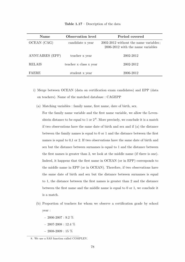
Table 1.17 – Description of the data

Name Observation level Period covered

OCEAN (CAG) candidate x year 2002-2012 without the name variables ;2006-2012 with the name variables

ANNUAIRES (EPP) teacher x year 2002-2012

RELAIS teacher x class x year 2002-2012

FAERE student x year 2006-2012

i) Merge between OCEAN (data on certification exam candidates) and EPP (data

on teachers). Name of the matched database : CAGEPP

(a) Matching variables : family name, first name, date of birth, sex.

For the family name variable and the first name variable, we allow the Leven-

shtein distance to be equal to 1 or 2 8. More precisely, we conclude it is a match

if two observations have the same date of birth and sex and if (a) the distance

between the family names is equal to 0 or 1 and the distance between the first

names is equal to 0,1 or 2. If two observations have the same date of birth and

sex but the distance between surnames is equal to 1 and the distance between

the first names is greater than 2, we look at the middle name (if there is one).

Indeed, it happens that the first name in OCEAN (or in EPP) corresponds to

the middle name in EPP (or in OCEAN). Therefore, if two observations have

the same date of birth and sex but the distance between surnames is equal

to 1, the distance between the first names is greater than 2 and the distance

between the first name and the middle name is equal to 0 or 1, we conclude it

is a match.

(b) Proportion of teachers for whom we observe a certification grade by school

year :

- 2006-2007 : 9.2 %

- 2007-2008 : 12.4 %

- 2008-2009 : 15 %

8. We use a SAS function called COMPLEV.

78

- 2009-2010 : 17.6 %

- 2010-2011 : 19.9 %

- 2011-2012 : 21.6 %

ii) We clean CAGEPP mainly by suppressing duplicate observations.

These duplicates are mainly due to (a) teachers who took different exams the same

year or (b) teachers who took different exams in different years. We only keep the

observation corresponding to the teacher’s actual certification level. For example,

if (a) in a given year, a teacher passed both the CAPES and the Agregation but

is registered in EPP as an Agrege, we only keep the observation corresponding

to her certification grade at the Agregation ; if (b) in 2007, a teacher passed the

CAPES but, in 2008, passed the Agregation, we keep, in 2007, the observation

corresponding to her certification grade at the CAPES but, in 2008, we only keep

the observation corresponding to her certification grade at the Agregation ; if (c) in

2007, a teacher passed the CAPES but, in 2008, took the Agregation and failed, we

only keep, both in 2007 and 2008, the observation corresponding to her certification

grade at the CAPES ; if (d) in 2007, a CAPES recipient took the Agregation but

failed, we suppress this observation ; if (e) a teacher passed both the CAPES of

mathematics and the CAPES of physics but is registered in EPP as Math teacher,

we only keep the observation corresponding to her certification grade at the CAPES

of mathematics.

We also suppress observations corresponding to teachers without any certification

status but teaching under a fixed-term contract (enseignants contractuels) who

took and failed a certification examination.

Merge between CAGEPP and RELAIS (data on teachers with the identification number

of their class(es))

1. Matching variable : teacher identification number

2. Proportion of teachers in CAGEPP for whom we observe the identification number of

their class(es) by school year :

- 2006-2007 : 93.9 %

- 2007-2008 : 85.2 %

- 2008-2009 : 81.2 %

79

- 2009-2010 : 82.3 %

- 2010-2011 : 79.6 %

- 2011-2012 : 80.7 %

The identification number of the class variable is missing in the FAERE database before

the 2009-2010 school year. Therefore, from the 2006-2007 school year to the 2008-2009

school year, we merge the FAERE database with the Scolarite database, in which the

identification number of the class variable is not missing.

1. Matching variables : date of birth, place of birth, school identification number, gender,

socioeconomic background of her mother, socioeconomic background of her father,

options and lunch status.

2. Proportion of students in FAERE before 2009-2010 for whom we observe the identifi-

cation number of their class : 90.8 %

Match between Junior high school teachers and Junior high school students

1. Matching variables : class identification number, grade identification number, school

identification number

2. Proportion of distinct Junior high school Math or French teachers in CAGEPP mat-

ched with their Junior high school students in FAERE by school year :

- 2006-2007 : 97.2 %

- 2007-2008 : 92.4 %

- 2008-2009 : 91.1 %

- 2009-2010 : 78.2 %

- 2010-2011 : 83.2 %

- 2011-2012 : 99.7 %

Match between Senior high school Math or French teachers and Senior high school stu-

dents

1. Matching variables : class identification number, grade identification number, school

identification number

2. Proportion of distinct Senior high school Math or French teachers in CAGEPP mat-

ched with their Senior high school students in FAERE by school year :

- 2006-2007 : 60.7 %

- 2007-2008 : 90.6 %

80

- 2008-2009 : 94.5 %

- 2009-2010 : 93.7 %

- 2010-2011 : 92.8 %

- 2011-2012 : 94.7 %

Our final samples cover teachers who have passed their certification examination bet-

ween school years 2005-2006 and 2010-2011. In particular, they do not include teachers

who passed their certification examination before 2005-2006 because the name variable–

essential to our merging procedure– is not available for this period. Our samples cover

students who have taken the DNB or the Baccalaureat between school years 2006-2007

and 2011-2012. More precisely, the two samples we analyse in this study are the following :

(i) ninth grade students (eleves de troisieme) matched to their Math and French tea-

chers. The sample is composed of students fulfilling the following conditions : we

observe both their Math and French teachers, both their Math teacher and their

French teacher passed the certification exam the same year (to control for diffe-

rences in teachers cohort composition–which the “masterisation” reform is likely

to make even more significant – and to make teachers’ certification grades as com-

parable as possible), we observe both their Math and French teachers certification

grade, classroom observation grade and school principal grade.

(ii) 12th grade Senior high school students (eleves de terminale) –hereafter Senior

high school students – matched to their Math and French teachers 9. The sample is

composed of student fulfilling the same conditions as those required for Junior high

students plus an additional one. This supplementary condition is that we observe

not only the student’s Baccalaureat test scores but also her DNB test scores. This

condition is actually only strictly required for the value-added analysis we perform

in section 5 but we also apply it for the sample on which is based the within

student, across topics analysis in order to guarantee the comparability of the two

approaches. The sample counts 8,295 students and 821 distinct teachers.

We focus on Math and French topics for three main reasons. The first reason is that Math

and French are the only topics (with History-Geography) for which externally graded test

scores are available and relatively comparable both for Junior and Senior high school. The

9. The French examination is actually taken in 11th grade (classe de premiere). Therefore, we matchstudents to their 11th grade French teacher.

81

second reason is that it enables us to improve the comparability of our results with those

of the literature – as most of the literature on teacher quality focuses on Math and En-

glish. The third reason is that Math and French are the two topics for which the threat of

teacher spillover effects across topics seems the less plausible. Koedel (2009) for example

suggests that teacher spillover effects between Math and English high school teachers are

not statistically significant. The threat of teacher spillover effects seems however, a priori,

more plausible for History-Geography for example, because students’ History-Geography

test scores also measure students’ reading and writing skills taught by their French tea-

cher. Students’ Math test scores (French test scores) seem less likely to be contaminated

by the effect of teachers teaching another topic than Math (French) to these students.

To facilitate the interpretation and the comparability of our results, we adopt several

normalizations. First, we normalize students test scores by subject and by year. Second, we

normalize the teacher certification grade by certification level, subject and year. Finally,

we normalize teacher pedagogical and school principal grades by year, certification level

and ranking on the wage scale, according the national grading tables presented in section

1 (Table 1.8 and Table 1.6). These normalizations imply that the estimated coefficients

can be interpreted as fractions of a standard deviation of the distribution of individual

scores.

82

Chapitre 2

Absence, Substitutability and

Productivity : Evidence from

Teachers

Worker absence is a frequent phenomenon but little is known on its effects on pro-

ductivity nor on organizations’ strategies to cope with this temporary disruptive event

through substitute workers. Using a unique French administrative dataset matching, for

each absence spell, each missing secondary school teacher to her substitute teacher, I

find that the expected loss in daily productivity from non-replaced days is on par with

replacing an average teacher with one at the 30th percentile of the teacher value-added

distribution. On average, substitute teachers are unable to mitigate this negative effect.

There is substantial heterogeneity by substitute teacher quality : higher quality substitute

teachers are able to compensate up to 25 % of this negative impact while lower quality

substitute teachers do not have any statistically significant impact. JEL : I2, J2, M51.

Keywords : absence, substitutability, productivity, teachers.

2.1 Introduction

Worker absence is frequent in many countries. For example, in the United Kingdom,

the United States and France alike, every year, two to three percent of annual work time

is lost due to worker absence (DARES, 2013 ; UK Office for National Statistics, 2014 ; US

Bureau of Labor Statistics, 2016). Despite the importance of this phenomenon, empirical

83

evidence on the causal effect of worker absence on productivity is scarce. 1 Even much

less is known on organizations’ strategies to cope with this temporary disruptive event

through worker substitution. When a worker is absent, how does it hurt her productivity ?

How easily can organizations mitigate this effect with substitute workers ? Several major

economic issues, from the impact of worker health and effort on productivity (Lazear

and Oyer, 2012) to the analysis of specific human capital (Jacobson et al., 1993 ; Altonji

and Williams, 2005 ; Gathmann and Schonberg, 2010) and its relationship with worker

substitutability (Stole and Zwiebel, 1996), depend on the answer to these questions.

I offer an empirical answer to these questions using a comprehensive administrative

French panel dataset covering the 2007-2015 period and matching, for each absence spell,

each missing secondary school teacher to her substitute teacher. This paper estimates,

for Math, French and History ninth grade teachers and their students : a) the effect of

the number of days of non-replaced teacher absence on student test scores ; b) how this

impact can be mitigated by the assignment of substitute teachers ; c) how the impact of

substitute teachers depends on their quality, measured by their type (tenured vs contract

teachers).

I implement a two-way fixed effect model with teacher and classroom-year fixed effects.

This model exploits the longititudinal dimension of the data with teacher-school fixed

effects. It also exploits the cross-sectional dimension of the data : in secondary school,

teachers are subject-specific and students stay with the same peers in the same classroom,

throughout the school year and for all subjects. This allows me to use variation within

classroom-year, across subject. I perform several robustness checks to confirm that the

results are not driven by a) reverse causality : teachers are more absent when assigned

to low performing students and it is more difficult to find quality substitution for this

type of students ; b) the fact that absences are only a reflection of poor on-the-job teacher

productivity ; c) or the fact that replaced absence spells are not comparable to non-

replaced ones.

Based on the analysis of more than 100,000 teachers and three millions students, I

show that teacher absence has a statistically negative impact on student test scores : the

expected loss in daily productivity from non-replaced days is on par with replacing an

1. To my best knowledge, there are only four papers covering this question : Miller et al (2008) ;Clotfelter et al. (2009) ; Duflo et al. (2012) ; Herrmann and Rockoff (2012)

84

average teacher with one at the 30th percentile of the teacher value-added distribution,

which is consistent with the very few studies on this question (Herrmann and Rockoff,

2012). The fraction of replaced absence spell does not have any statistically significant

compensating effect. However, when I make the distinction between the two type of sub-

stitute teachers, I find that one additional replaced day with a tenured substitute teacher

(as opposed to a missed day at school) mitigates 26 % of the marginal impact of non-

replaced days. The marginal impact of a replaced day with a contract teacher (as opposed

to a missed day at school) is not statistically significant.

I also estimate heterogeneity by teacher and absence spell characteristics to provide

suggestive evidence on the underlying mechanisms highlighted in a conceptual framework.

I first investigate the role of the gap in general human capital between the regular and

the substitute teachers. The main prediction from the conceptual framework is that the

larger this gap, the smaller the mitigating effect of substitution. I use teacher experience

as a measure of general human capital because the link between teacher experience and

teacher productivity is well established in the literature (see Koedel et al., 2015 for a re-

view). I find that the mitigating effect of tenured substitution is not significantly impacted

by the experience gap. This suggests that the results cannot be entirely explained by this

mechanism. I then investigate the role of the specific human capital gap : teaching re-

quires specific human capital which can be acquired only through prolonged and repeated

interactions with students. The role of this mechanism is supported by the heterogeneity

analysis by month of the year : absence spells happening at the end of the school year

have a larger impact than those happening at the beginning of the year, when the specific

human capital gap between the substitute and the regular teachers is smaller.

This paper contributes to several strands of the literature. First, this paper contributes

to an emerging empirical literature on worker substitutability. Hensvik and Rosenqvist

(2016) show that worker sickness absence is lower in positions with few internal substitute

and give evidence that firms try to keep absence low in positions with few internal substi-

tute. Jager (2016) analyzes the effect of unexpected worker deaths in the German private

sector and shows these worker exits on average raise the remaining workers’ wages and

retention probabilities. While these papers use wage and retention as proxies for worker

productivity, I measure it based on an actual and multidimensional output, student out-

comes. I can rely on an important literature which consistently finds teachers to be the

85

most important determinant of student outcomes, both in the short and long run (Ro-

ckoff, 2004 ; Rivkin, Hanushek and Kain, 2005 ; Chetty, Friedman and Rockoff, 2014a ;b).

Moreover, because teaching is a complex, multidimensional task, based on direct, perso-

nal and prolonged interactions with the “output” (students), it requires specific human

capital (student-specific, grade-specific etc., see Ost, 2014), which makes it particularly

well suited to the analysis of the relationship between human capital specificity and sub-

stitutability.

Second, it contributes to the very small literature on the effect of worker absence on

productivity (Miller et al., 2008 ; Clotfelter et al., 2009 ; Duflo et al., 2012 ; Herrmann

and Rockoff, 2012). This literature focuses on teachers and finds that the expected loss

in daily productivity from teacher absence is on par with replacing a teacher of average

productivity with one at the 10th-20th percentile of productivity. One of the most im-

portant limitation of this literature is that it does not provide any empirical evidence on

the impact of substitute teachers and the channels through which teacher absence affects

students. A forthcoming paper by Schiprowski (2020) provides evidence on the impact

of absence in a different context, unemployment insurenace caseworkers, and finds that

individuals who lose a meeting with their caseworker stay unemployed 5% longer. This

paper does not discuss however the impact of non-replacement and substitution.

Third, this paper contributes to the small literature on contract teachers, which focuses

on developing countries. The main paper on this question is Duflo et al.(2012), which

shows that, in Kenyan primary schools, contract teachers are more efficient than regular

teachers when their hiring is more closely monitored and they have higher incentives

to exert effort. The French context analyzed in this paper is very different because the

requirements to become a contract teacher are very low and contract teachers do not have

higher incentives than regular teachers to exert effort.

Finally, this paper contributes to the literature on instruction time (Pischke, 2007 ;

Lavy, 2015). This literature finds that longer instructional time has a positive impact on

student test scores and one-time grade progression. While these papers focus on variations

in planned instruction time defined by law, I go a step further and analyze the impact on

student outcomes of variations in the actual amount of instruction hours, and of variations

with whom they are actually spent (regular or substitute teacher).

The remainder of the paper is organized as follows. Section 2 describes the French

86

educational context, highlighting its relevance to the analysis of worker absence and sub-

stitutability. Section 3 presents a highly stylized conceptual framework to illustrate the

mechanisms through which teacher absence and substitution affect student outcomes.

Section 4 presents the data and some descriptive statistics. Section 5 exposes the empiri-

cal strategy, section 6 the baseline results and section 7 the robustness checks. Section 8

shows the hetergoneity analysis. Section 9 concludes.

2.2 Institutional Setting

To provide context for the empirical analysis, this section describes the main relevant

features of the French educational system. It focuses more specifically on describing the

different types of teachers and the teacher assignment system.

2.2.1 Secondary School Teachers in France

The public French educational system is highly centralized. Schools have little au-

tonomy and they are in particular, all required to follow the same national curriculum.

School principals cannot hire nor fire their teachers. The French territory 2 is decomposed

in 25 large regions, called academies (hereafter regions).

Secondary school teachers are selected through a subject-specific national competitive

examination, which is demanding academically and has low passing rates (between 15 and

30 %). There are two main certification levels : basic, called CAPES (Certificat d’apti-

tude au professorat de l’enseignement du second degre) and advanced, called Agregation.

Conditional on passing this examination, teachers become civil servants and are managed

by the government. They have a permanent position and cannot be fired.

Certified teachers are assigned via a centralized point-based system (called SIAM,

Systeme d’information et d’aide aux mutations) with two rounds : the inter-regional round

and the regional round. Candidates submit a rank-ordered list of choices and are assigned

according to a modified version of the school-proposing Deferred Acceptance mechanism

(Combes, Tercieux and Terrier, 2016). Teachers’ priorities are mostly determined by their

number of years of experience. Every year, i) new teachers and tenured teachers who

want to change region apply to the inter-regional mobility round ; ii) participants of the

2. This paper focuses on mainland France and does not analyse its overseas territories.

87

inter-regional mobility round, and tenured teachers who want to change school within

their region, apply to the intra-regional mobility round.

Teachers’ wage is set through a national wage scale based on teachers’ number of

years of experience and certification level (none, basic and advanced). For example, the

gross wage of a teacher with the basic certification level and a year of experience is

approximately 2,000 euros per month. Wages do not vary across schools and do not

depend on output.

Secondary school teachers are subject-specific : each subject is taught by a different

teacher. The legal working week is 15 hours for teachers with an advanced certification

level and 18 hours for teachers with a basic certification level. Students are not tracked

by major nor ability. Students stay in the same class, with the same peers throughout

the school year and in all subjects. For ninth graders, a typical week consists in 29 school

hours, distributed across 11 teachers– subjects, among which 4 hours of French, 3.30

hours of Mathematics, and 3.30 hours of History 3 . At the end of 9th grade, students

take a national and externally graded examination called Diplome national du Brevet in

three subjects : French, Math and History. This exam takes place in the very last days of

June/early days of July.

2.2.2 Teacher Absence Leave Regulation

Teachers are fully paid during the first three months of their absence leave for minor

illness, and during the first to third year of their leave for serious illness. After this period,

they receive half of their regular pay. Teachers are fully paid during their maternity leave,

which can last from 16 to 46 weeks depending on the order of the birth. Paternity leaves

are also fully paid and can last from 11 to 18 days. Teacher can also take fully paid leave

for professional reasons such as training, meetings, participation to an examination board

etc.. There is no limitation in the number of days of paid absence each teacher can take

per year.

3. The rest of the hours are distributed between Foreign Languages (5h30), Science (4h30), Sport(3h)and Art (2h), see http ://www.education.gouv.fr/cid80/les-horaires-par-cycle-au-college.html

88

2.2.3 Teacher Substitution Procedure

Teacher absences are not systematically replaced in France. Overall, the probability of

replacement depends on the length of the absence spell and the availability of substitute

teachers. Absences are handled by the regional educational authority (rectorat). There

are no official precise criteria : regional educational authorities are simply asked to give

priority to long term absences (IGEN, 2011).

In practice, when a teacher is absent, she has to notify her school principal, who then

notifies the region via an online form, whatever the length of the absence spell. Regional

educational authorities assign substitute teachers manually.

2.2.4 Substitute Teachers

Tenured Substitute Teachers. Certified teachers can ask to become substitute

teachers during the intra-regional mobility round of the centralized teacher assignment

procedure but most tenured substitutes (Titulaires sur zone de remplacement) are tea-

chers who participated to the inter-regional mobility round and failed to obtain one of

their choices in the intra-regional mobility round (IGAENR, 2015). They are assigned to

a reference school called etablissement de rattachement administratif (RAD), and can be

called to replace absent teachers in any school located in an geographical area called zone

de remplacement. 4 There are around 250 zones de remplacement in France. Tenured sub-

stitute teachers’ wages do not depend on the number of substitution they perform nor on

the number of hours they work. Their wage is mainly fixed and equal the regular teachers’

wage. As explained above, there is no clear rule for the assignment of tenured substitute

teachers. Regional educational authorities, which are in charge of the assignment and do

it manually, are simply given the general guideline to give priority to long absence spells

(IGEN, 2011). Substitute teachers do not have the possibility to refuse an assignment. 5

Contract Teachers. When there is a shortage of available tenured substitute tea-

chers, regions hire contract teachers on the spot. Contract teachers are not hired via the

same procedure as certified teachers. Candidates apply directly to regional educational

authorities via an online platform. 6 To be eligible, they must hold a Bachelor’s degree

4. Decret 99-823 du 17 septembre 19995. This is different in other countries such as the United States, see Gershenson (2012)6. This online platform is called, depending on the region, either SIATEN (Systeme d’information

89

and have no criminal record. Candidates submit their resume, cover letter and, in some

regions, their geographical preferences. The selection process is managed by regional pro-

fessional inspectors. In general, professional inspectors are experienced teachers. They

screen candidates based on their online application and conduct interviews. Successful

candidates are hired on a short term contract (Contrat a duree determinee) of maximum

a year. Contract teachers’ wage depends on their degree (High school degree, Bachelor’s,

Master’s or more), their professional experience, and on their region. 7 For example, the

gross wage of a contract teacher in Paris, with a Bachelor’s degree and a year of experience

is 1699 / month.

2.3 Conceptual Framework

This section presents the main intuitions and predictions of a highly stylized concep-

tual framework illustrating how teacher absences can impact teacher productivity and

how this impact can be mitigated or exacerbated by substitute teachers. This detailed

conceptual framework is presented in appendix (section 2.11).

This framework builds on the education production function framework. Teacher pro-

ductivity depends on her ability, general human capital (including professional experience)

and, importantly, student-specific human capital. The basic intuition of student-specific

human capital is that the longer teachers spend time with the specific students they are

assigned to, the better they are at teaching them. This may be because they get to know

students and adjust to them, and also have more time to implement a long-term instruc-

tional strategy. Existing suggestive empirical evidence back this intuition. Duflo, Dupas

and Kremer (2011) suggest teachers adjust the level at which they teach in response

to changes in class composition. Herrmann and Rockoff (2012) find daily productivity

losses from absence decline with the length of an absence spell, consistent with substitute

teachers learning on the job.

The main predictions of this conceptual framework are the following. Teacher absence

can impact teacher productivity through different channels, depending on whether the

absent teacher is replaced, and on the quality of the substitute teacher :

des agents temporaires de l’Education nationale) or ACLOE (Application de gestion des candidatures enligne)

7. http ://vocationenseignant.fr/devenir-enseignant-contractuel-ou-vacataire-mode-d-emploi

90

1. If the regular teacher is absent and no substitute teacher is assigned, teacher ab-

sence can impact productivity through the loss of instruction time and the amount

of student-specific capital the regular teacher loses during her absence. The higher

the regular teacher productivity, the bigger the impact of the loss of instruction

time ;

2. If the regular teacher is absent and a substitute teacher is assigned, the main

channels are :

- the difference in ability and experience between the regular and the substitute

teachers ;

- how fast substitute teachers gain student-specific human capital ;

- the amount of student-specific capital the regular teacher loses during her ab-

sence.

2.4 Data and Descriptive Statistics

This section presents the administrative data on regular teachers, substitute teachers

and their students. Its main advantage is that it is a comprehensive panel data matching

each teacher to her students, and each absent teacher to her substitute teacher for each

absence spell. The main estimation sample is composed of all ninth grade students and

their Math, French and History teachers from 2007 to 2015. This corresponds to 5,233

schools, 101,479 teachers and 3,259,290 students. This section also provides the descriptive

statistics necessary to understand how absence and substitution spells are distributed

across teachers and schools.

2.4.1 Data

This paper relies on administrative data from the French ministry of Education cove-

ring the whole country and school years 2005-2006 through 2014-2015. I focus on Math,

French and History teachers matched to their ninth grade students. A precise description

of the data is found in appendix (section ??). I exploit four main set of data :

- individual data on students including an encrypted national identification number,

gender, financial aid status, parents’ occupation, the identification number of their

school and of their class. A separate database also includes their test scores at the

91

end of 9th grade examination in French, Math and History, which I standardize

by year and region.

- individual data on teachers including national identification number, date of birth,

gender, number of year of teaching experience, teaching subject, identification num-

ber of their assignment, and the identification number of the school and of the class

they teach. The two latter variables are used to match each teacher to her students.

I take into account, throughout the paper, only open business days and remove

holidays and weekends.

- data on teachers’ absence spells : regional identification number of the absent

teacher ; day, month and year of the absence spells ; detailed cause of absence

(minor illness, maternity leave, training etc.) ; region identification number.

- data on teachers’ assignment spells : region identification number of the substitute

teacher, day, month and year of the assignment spells ; identification number of

their assignment ; national identifying number of the school. The match between

the absent and the substitute teachers is made on the identification number and

dates of their respective assignment spells. As for absence spells, I take into ac-

count, throughout the paper, only open business days and remove from absence

spells holidays and weekends.

2.4.2 Summary Statistics

Distribution of Absence Spells. Each year, 55 percent of teachers do not take any

absence leave (Figure 2.1). Around half of teachers who are absent take only one absence

spell. The majority of absence spells are health-related : 50 % for minor sickness, 10 %

for long term illness, 3 % for maternity leave, 2 % for maternity leave extension (in case

of a difficult pregnancy or childbirth) and 1 % for professional illness ( Figure 2.8a).

Teachers are absent 13.14 days per year on average, which represents around 7 % of

the yearly instructional time. Figure 2.3 shows the cumulative distribution of the number

of instructional days of absence per absence spell. More than 36 % of absence spells last

only one day. The distribution of absence spells is right-skewed, with 80 % of absence

spells lasting less than 20 days.

Distribution of Substitution Spells. In 2015, the number of replaced days is equal

to 10 days per year, which means that around 75 % of absent days are replaced (Figure

92

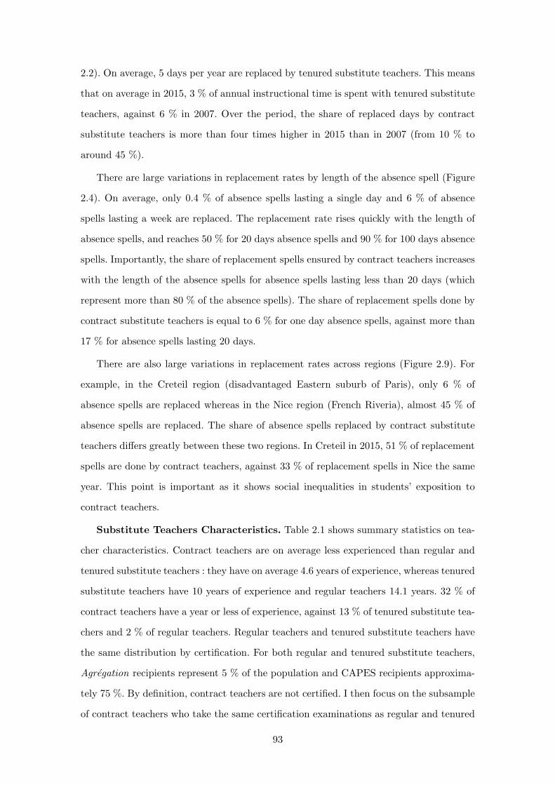
2.2). On average, 5 days per year are replaced by tenured substitute teachers. This means

that on average in 2015, 3 % of annual instructional time is spent with tenured substitute

teachers, against 6 % in 2007. Over the period, the share of replaced days by contract

substitute teachers is more than four times higher in 2015 than in 2007 (from 10 % to

around 45 %).

There are large variations in replacement rates by length of the absence spell (Figure

2.4). On average, only 0.4 % of absence spells lasting a single day and 6 % of absence

spells lasting a week are replaced. The replacement rate rises quickly with the length of

absence spells, and reaches 50 % for 20 days absence spells and 90 % for 100 days absence

spells. Importantly, the share of replacement spells ensured by contract teachers increases

with the length of the absence spells for absence spells lasting less than 20 days (which

represent more than 80 % of the absence spells). The share of replacement spells done by

contract substitute teachers is equal to 6 % for one day absence spells, against more than

17 % for absence spells lasting 20 days.

There are also large variations in replacement rates across regions (Figure 2.9). For

example, in the Creteil region (disadvantaged Eastern suburb of Paris), only 6 % of

absence spells are replaced whereas in the Nice region (French Riveria), almost 45 % of

absence spells are replaced. The share of absence spells replaced by contract substitute

teachers differs greatly between these two regions. In Creteil in 2015, 51 % of replacement

spells are done by contract teachers, against 33 % of replacement spells in Nice the same

year. This point is important as it shows social inequalities in students’ exposition to

contract teachers.

Substitute Teachers Characteristics. Table 2.1 shows summary statistics on tea-

cher characteristics. Contract teachers are on average less experienced than regular and

tenured substitute teachers : they have on average 4.6 years of experience, whereas tenured

substitute teachers have 10 years of experience and regular teachers 14.1 years. 32 % of

contract teachers have a year or less of experience, against 13 % of tenured substitute tea-

chers and 2 % of regular teachers. Regular teachers and tenured substitute teachers have

the same distribution by certification. For both regular and tenured substitute teachers,

Agregation recipients represent 5 % of the population and CAPES recipients approxima-

tely 75 %. By definition, contract teachers are not certified. I then focus on the subsample

of contract teachers who take the same certification examinations as regular and tenured

93

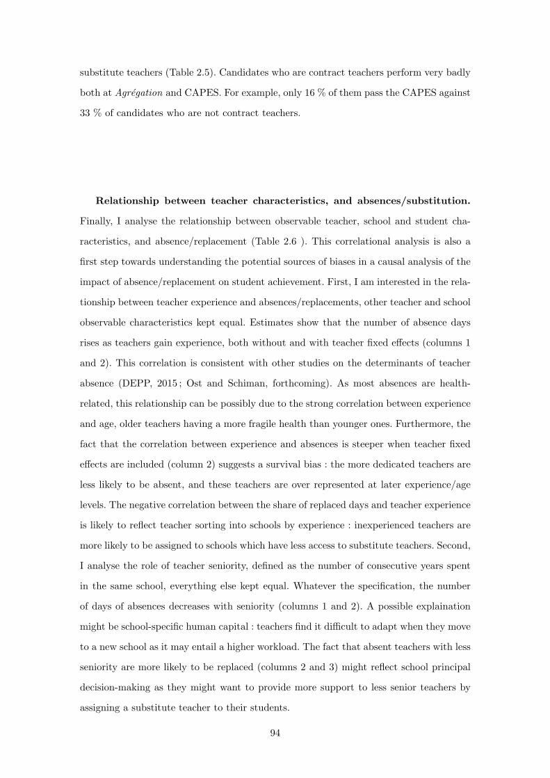
substitute teachers (Table 2.5). Candidates who are contract teachers perform very badly

both at Agregation and CAPES. For example, only 16 % of them pass the CAPES against

33 % of candidates who are not contract teachers.

Relationship between teacher characteristics, and absences/substitution.

Finally, I analyse the relationship between observable teacher, school and student cha-

racteristics, and absence/replacement (Table 2.6 ). This correlational analysis is also a

first step towards understanding the potential sources of biases in a causal analysis of the

impact of absence/replacement on student achievement. First, I am interested in the rela-

tionship between teacher experience and absences/replacements, other teacher and school

observable characteristics kept equal. Estimates show that the number of absence days

rises as teachers gain experience, both without and with teacher fixed effects (columns 1

and 2). This correlation is consistent with other studies on the determinants of teacher

absence (DEPP, 2015 ; Ost and Schiman, forthcoming). As most absences are health-

related, this relationship can be possibly due to the strong correlation between experience

and age, older teachers having a more fragile health than younger ones. Furthermore, the

fact that the correlation between experience and absences is steeper when teacher fixed

effects are included (column 2) suggests a survival bias : the more dedicated teachers are

less likely to be absent, and these teachers are over represented at later experience/age

levels. The negative correlation between the share of replaced days and teacher experience

is likely to reflect teacher sorting into schools by experience : inexperienced teachers are

more likely to be assigned to schools which have less access to substitute teachers. Second,

I analyse the role of teacher seniority, defined as the number of consecutive years spent

in the same school, everything else kept equal. Whatever the specification, the number

of days of absences decreases with seniority (columns 1 and 2). A possible explaination

might be school-specific human capital : teachers find it difficult to adapt when they move

to a new school as it may entail a higher workload. The fact that absent teachers with less

seniority are more likely to be replaced (columns 2 and 3) might reflect school principal

decision-making as they might want to provide more support to less senior teachers by

assigning a substitute teacher to their students.

94

2.5 Empirical Strategy

This section describes the empirical strategy implemented to identify the impact of ab-

sence and substitution on student achievement. I implement a two-way fixed effect model

with teacher-school and classroom fixed effects. I present the main empirical challenges

and how they are addressed by this empirical strategy.

2.5.1 Empirical Strategy

The main empirical challenge raised by the estimation of the impact of teacher ab-

sence/substitution is the non-random teacher- student matching. As suggested by Table

2.6, absences and substitution can be correlated with observed and unobserved teachers’

characteristics which can have a direct impact on student achievement. This table confirms

results from the literature establishing the statistically significant relationship between

teacher experience, her student socioeconomic background and her number of days of ab-

sence (e.g. Ost and Schiman, forthcoming). Futhermore, there is a statistically significant

relationship between teacher substitution and her student socioeconomic background,

experience and other teacher characteristics kept equal. Low quality teachers can be sys-

tematically assigned to low achieving students.

To deal with these issues, I implement a two way fixed effect model with teacher

and classroom fixed effects. First, I exploit the longititudinal dimension of the data with

teacher-school fixed effects, which control for both observed and unobserved teacher fixed

characteristics (Miller et al., 2008 ; Herrmann and Rockoff, 2012). Therefore, I exploit

within teacher, across years variations in the number of days of absence and in the number

of replaced days. This source of variation has already been exploited in the previous studies

on the impact of teacher absences on student achievement (Miller, 2008 ; Herrmann and

Rockoff, 2012). However, a major concern for the validity of this strategy is unobserved

variation in student ability, which can impact both teacher absences and replacement and

student test scores. This is why I go a step further and take advantage of the fact that,

in secondary school, teachers are subject-specific and that students stay with the same

peers in the same classroom, throughout the school year and in every subject. This allows

me to also exploit variation within classroom-year, across subjects. Formally, this model

95

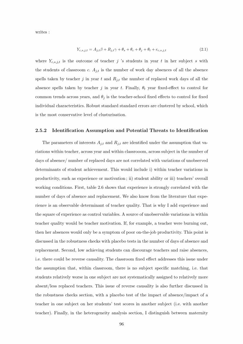
writes :

Yc,s,j,t = Aj,tβ +Rj,tγ + θs + θc + θj + θt + ec,s,j,t (2.1)

where Yc,s,j,t is the outcome of teacher j ’s students in year t in her subject s with

the students of classroom c. Aj,t is the number of work day absences of all the absence

spells taken by teacher j in year t and Rj,t the number of replaced work days of all the

absence spells taken by teacher j in year t. Finally, θt year fixed-effect to control for

common trends across years, and θj is the teacher-school fixed effects to control for fixed

individual characteristics. Robust standard standard errors are clustered by school, which

is the most conservative level of clusturisation.

2.5.2 Identification Assumption and Potential Threats to Identification

The parameters of interests Aj,t and Rj,t are identified under the assumption that va-

riations within teacher, across year and within classrooom, across subject in the number of

days of absence/ number of replaced days are not correlated with variations of unobserved

determinants of student achievement. This would include i) within teacher variations in

productivity, such as experience or motivation ; ii) student ability or iii) teachers’ overall

working conditions. First, table 2.6 shows that experience is strongly correlated with the

number of days of absence and replacement. We also know from the literature that expe-

rience is an observable determinant of teacher quality. That is why I add experience and

the square of experience as control variables. A source of unobservable variations in within

teacher quality would be teacher motivation. If, for example, a teacher were burning out,

then her absences would only be a symptom of poor on-the-job productivity. This point is

discussed in the robustness checks with placebo tests in the number of days of absence and

replacement. Second, low achieving students can discourage teachers and raise absences,

i.e. there could be reverse causality. The classroom fixed effect addresses this issue under

the assumption that, within classroom, there is no subject specific matching, i.e. that

students relatively worse in one subject are not systematically assigned to relatively more

absent/less replaced teachers. This issue of reverse causality is also further discussed in

the robustness checks section, with a placebo test of the impact of absence/impact of a

teacher in one subject on her students’ test scores in another subject (i.e. with another

teacher). Finally, in the heterogeneity analysis section, I distinguish between maternity

96

leaves and other type of absences. Indeed, maternity leave is the reason of absence most

likely to be unrelated to within teacher variations in motivation or burning out, student

ability or working conditions.

Another type of potential threat for identification is more specific to the replacement

parameters. These parameters would not be identified if the type of absence spells that

are replaced were not comparable to those who are not. For example, absences planned

in advance may be more likely to be replaced than absences that are unexpected. In that

case, the impact of replacement may be biased. Teachers who know in advance they are

going to be missing a certain period of time can prepare their absence by giving guidelines

to their substitute, specific homework to their students etc. In particular, the analysis of

the impact of the assignment of tenured substitute teachers or contract substitute teachers

would be biased if tenured substitute teachers where assigned to different type of absence

spells, e.g. of different length, period of the year or reason, than contract substitute

teachers. This is all the more relevant since the summary statistics (Figure 2.4) shows

that, for absence spells lasting less than 20 days (more than 80 % of the absence spells),

the share of replacement spells done by contract teachers increases with the length of the

absence spell. I tackle this issue by performing several heterogeneity analyzes, in particular

by length of absence spell and reason of absence. More specifically, distinguishing between

maternity leaves and other types of absence can be fruitful because maternity leaves are

the absences that are the most likely to be planned long in advance.

Finally, it is important to note that this identification strategy relies on across subject

variations in the number of absent/replacement days. The estimated parameters give

the average effect across subjects and rely on the assumption of a constant effect across

subjects. I relax this assumption in the heterogeneity analysis by subject (section 8.2).

2.6 Baseline Results

The main results show one additional non-replaced day of absence reduces student test

scores by 0.03 % of a standard deviation. On average, substitute teachers are unable to

have any statistically significant mitigating effect. This average effects masks substantial

heterogeneity : tenured substitute teachers are able to mitigate up to 25 % of this negative

effect whereas contract teachers have no statistically significant mitigating effect.

97

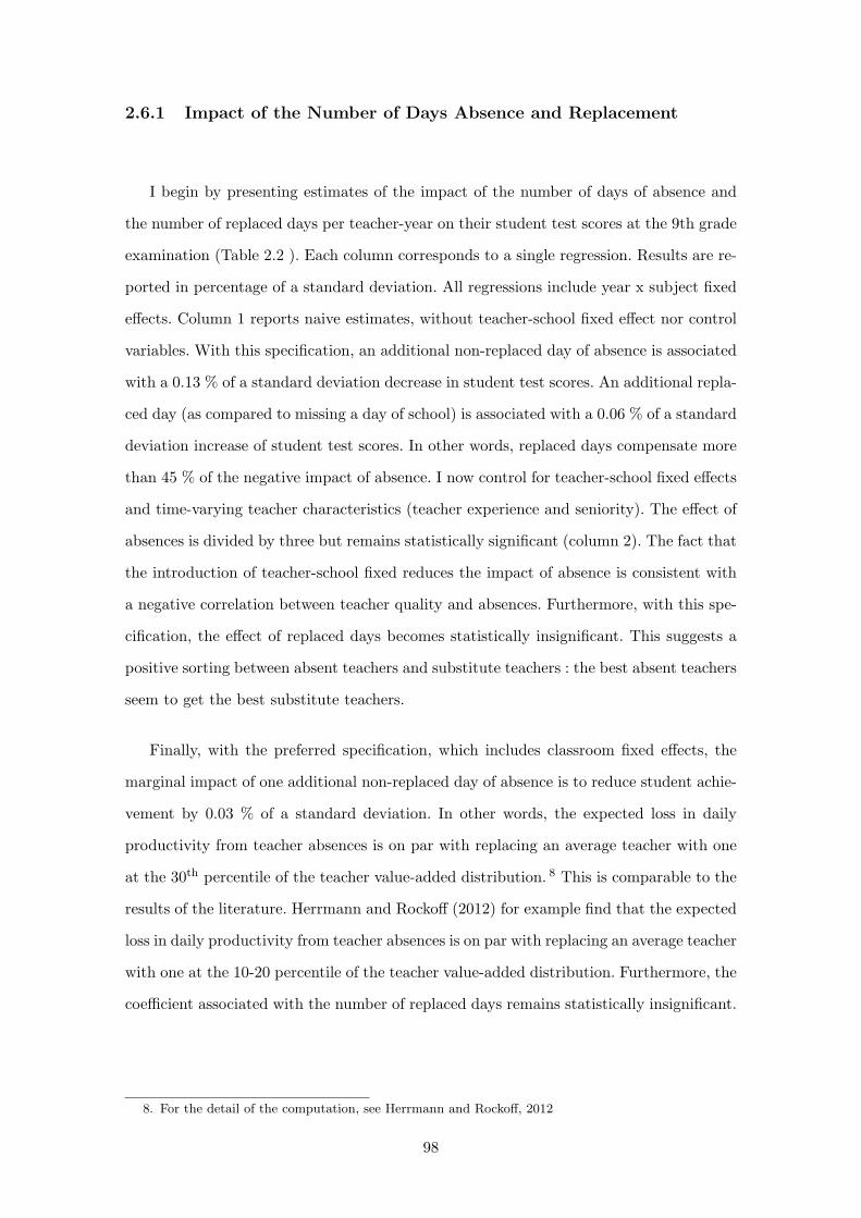
2.6.1 Impact of the Number of Days Absence and Replacement

I begin by presenting estimates of the impact of the number of days of absence and

the number of replaced days per teacher-year on their student test scores at the 9th grade

examination (Table 2.2 ). Each column corresponds to a single regression. Results are re-

ported in percentage of a standard deviation. All regressions include year x subject fixed

effects. Column 1 reports naive estimates, without teacher-school fixed effect nor control

variables. With this specification, an additional non-replaced day of absence is associated

with a 0.13 % of a standard deviation decrease in student test scores. An additional repla-

ced day (as compared to missing a day of school) is associated with a 0.06 % of a standard

deviation increase of student test scores. In other words, replaced days compensate more

than 45 % of the negative impact of absence. I now control for teacher-school fixed effects

and time-varying teacher characteristics (teacher experience and seniority). The effect of

absences is divided by three but remains statistically significant (column 2). The fact that

the introduction of teacher-school fixed reduces the impact of absence is consistent with

a negative correlation between teacher quality and absences. Furthermore, with this spe-

cification, the effect of replaced days becomes statistically insignificant. This suggests a

positive sorting between absent teachers and substitute teachers : the best absent teachers

seem to get the best substitute teachers.

Finally, with the preferred specification, which includes classroom fixed effects, the

marginal impact of one additional non-replaced day of absence is to reduce student achie-

vement by 0.03 % of a standard deviation. In other words, the expected loss in daily

productivity from teacher absences is on par with replacing an average teacher with one

at the 30th percentile of the teacher value-added distribution. 8 This is comparable to the

results of the literature. Herrmann and Rockoff (2012) for example find that the expected

loss in daily productivity from teacher absences is on par with replacing an average teacher

with one at the 10-20 percentile of the teacher value-added distribution. Furthermore, the

coefficient associated with the number of replaced days remains statistically insignificant.

8. For the detail of the computation, see Herrmann and Rockoff, 2012

98

2.6.2 Impact of the Number of Days of Replacement by Type of Sub-

stitute Teachers

The above results seems to suggest that substitute teachers are, on average, unable

to compensate the negative impact of teacher absences. Table 2.3 shows that, actually,

the impact of replaced days largely depends on the type of substitute teachers. With the

preferred specification (column 3), tenured substitute teachers are able to mitigate more

than 25 % of the marginal impact of absences. On the other hand, the marginal impact

of a replaced day with a contract teacher (as compared to missing a day of school) is not

statistically significant.

This result suggests that substitute teacher quality plays an important role in the

mitigating impact of substitution. This result is consistent with the conceptual framework

showing that one of the main mechanisms underlying the impact of teacher absence is the

human capital gap between the regular and the substitute teachers.

2.7 Robustness Checks

This section aims at adressing the main potential threats to identification. I discuss

three main threats to identification : reverse causality, absence as a symptom of poor

on-the-job teacher quality, non-comparability of replaced absences with non-replaced ab-

sences.

2.7.1 Threat I : Reverse Causality

Placebo test with students’ teacher in another subject. A concern for the

validity of the baseline results is that the bias caused by unobserved variations in student

ability, which can impact both teacher absences and replacement and student test scores.

To address this concern, we test whether absences and replacements of a teacher in one

subject impact her students’ test scores in another subject (i.e. with another teacher). If

the baseline results were driven by student ability, then the absence days and replaced days

of the Math teacher of student i would be significantly correlated with student test scores

in French. Table 2.9 reports regression estimates of the effect of absence and replaced

days of the “other subject” teacher of student i on student test scores in 9th grade. Each

column-panel corresponds to a single regression. This table shows that Math absence and

99

replacement days are not significantly related to student achievement in French and in

History. This is also true for French absence and replacement days on Math and History

test scores ; and of History absence and replacement days on French and Math test scores.

Thus, this placebo test gives strong evidence in favour of the robustness of the baseline

results.

2.7.2 Threat II : Absence as a Symptom of Poor On-the-job Teacher

Quality

Previous and Following Year Absences and Substitution. I also give evidence

against the idea that the baseline results are driven by the fact that absences are only a

symptom of poor on-the-job teacher quality. If, for example, the impact of absence were

only capturing the fact that absent teacher were burning out, then previous and following

absences would have a statistically significant impact. Table 2.10 reports a placebo test

of the effect of absence and replacement of the previous year ( t − 1) and following year

( t + 1) of teacher j on student test scores in 9th grade with teacher j during the year

t. Each column corresponds to a different regression. All regressions correspond to the

preferred specification. This table shows absent days and replacement day of years t− 1

and t+1 do not have any statistically significant impact on student achievement in year t.

Therefore, it does not seem that the baseline result are biased by poor on-the-job teacher

performance.

Absences During the Holidays. Teachers who fall sick or pregnant during the

school holidays (days when they do not have class) or during summer time have the

possibility to declare these days in order to have these absence days transferred during

school time 9. These absence spells represent around 1 % of the observations. Half of them

are maternity leaves happening over the summer. Table 2.7 shows regression estimates of

the marginal impact of one day of absence during holidays. It shows that these estimates

are not statistically significant. Therefore, this suggests that the baseline estimates are

not driven by that the baseline estimates are not driven by the fact that absence would

be a symptom of poor on-the-job teacher quality.

9. Source : https ://www.service-public.fr/particuliers/vosdroits/F2481

100

2.7.3 Threat III : Replaced Absences are not Comparable to non-replaced

Absences

Heterogeneity by Reason of Absence. Table 2.8 reports regression estimates by

reason of absence. This table corresponds to a single regression. I make the distinction

between absence spells for maternity leave and non maternity leave absence spells. As

discussed in the empirical strategy, the reason for this distinction is that maternity leave

absence spells are less likely to be determined by within teacher variations in teacher

quality, student ability or working conditions. Furthermore, maternity leaves are more

likely to be planned long in advance. We observe that the marginal impact of absence for

maternity leave is to reduce student test scores by 0.05 % of a standard deviation. The

impact of absence for non maternity leave absences is similar. The impact of replacement

by a tenured substitute teacher, for both maternity leave and non maternity leave ab-

sences, is to mitigate 30 - 35 % of the negative impact of absence. The fact that estimates

for maternity leave absence spells and non maternity absence spells are very similar gives

strong support for the robustness of the baseline results.

2.8 Heterogeneity Analysis

Having established the impact of teacher absence and substitution on student achieve-

ment, I then estimate heterogeneity across teachers, absence spells and school characteris-

tics. This heterogeneity analysis aims at shedding light on the mechanisms underlying the

main results and giving suggestive evidence on the conceptual framework’s predictions.

2.8.1 Heterogenity by Length of Absence

I start by analysing the marginal impact of one additional non-replaced day by length

of absence spell. The idea is to test whether the disruptive impact of teacher absence,

predicted by the conceptual framework, decreases with length of absence spell. Figure 2.5

reports regression estimates of the effect of absence and replaced days on student test

scores in 9th grade by length of absence spell. The marginal impact of one additional day

of absence decreases with the length of absence spells. The marginal impact of absence is

to reduce student achievement by around 0.1 % of a standard deviation for absence spells

lasting one day whereas it is equal to less than 0.05 % of a standard deviation for absence

101

spells lasting 10 days.

This decreasing marginal impact of non-replaced days may be due to alternative com-

pensating strategies from students or their parents (private tutoring for example) as ab-

sence spells get longer.

2.8.2 Heterogeneity by Subject

According to the conceptual framework, the main channel through which non-replaced

days impact student achievement is the loss of instructional time. In this framework, the

higher the regular teacher productivity, the bigger the impact of loss of instructional time

and thus the bigger the impact of non-replaced days.

I investigate this mechanism by leveraging the research design to estimate heteroge-

neity across teaching subject. It is well established in the literature that teacher produc-

tivity varies greatly by subject. In particular Math teachers value-added is higher than

in other subjects (see Chetty et al., 2014 for the latest evidence). Therefore, according to

the conceptual framework, the negative impact of non-replaced days in Math should be

higher than in the other two subjects.

Figure 2.6 reports regression estimates by teaching subject. The marginal impact of

one additional day of non-replaced absence in Math is to reduce student achievement by

0.08 % of a standard deviation. In French and History, this impact is equal to 0.04 % of

a standard deviation. The fact that absences have a larger impact in Math than in other

subjects is consistent with the literature (Miller et al., 2008 ; Herrmann and Rockoff,

2012). This result is consistent with the intuition that the higher the teacher value-added,

the higher the impact of absence.

2.8.3 Heterogeneity by the Experience Gap between the Substitute and

the Regular Teacher

Another major prediction of the conceptual framework is that the mitigating effect

of substitution depends on the general human capital gap between the regular and the

substitute teachers. I use teacher experience as a measure of general human capital because

the link between teacher experience and teacher productivity is well established in the

literature (see Koedel et al., 2015 for a review). According to the conceptual framework,

the larger the experience gap between the regular and the substitute teacher, the smaller

102

the mitigitating impact of substitution.

Table 2.4 reports estimates from interacting the number replaced days by each type

of substitute teachers and the experience gap between the regular and the substitute tea-

chers. It mainly shows that the mitigating effect of tenured substitution is not significantly

impacted by the experience gap, suggesting the existence of other mechanisms.

2.8.4 Heterogeneity by Month of the School Year

The last mechanism I explore is the role of the student-specific human capital gap

between the regular and the substitute teachers. According to this framework, the larger

this gap, the bigger the impact of absence. I analyse the impact of non-replaced days by

month of absence spell to provide suggestive evidence on this mechanism. The intuition is

that the student-specific human capital gap between the regular and substitute teachers

is larger in the end of the school year than in the beginning : in September, both regular

and substitute teachers have limited knowledge of students and the classroom dynamics,

but as the regular teacher interacts more and more with her students, she gains more and

more specific human capital.

Figure 2.7 reports estimates of the impact of the number of days/substitution by

month of the beginning of the absence spell. The three graphs correspond to a single

regression with the preferred specification. The graph 2.7a shows the seasonality of the

marginal impact of absence (controlling for the number of replaced days with tenured

substitute and contract substitute). The marginal impact of absence starting in September

is not statistically significant at the five percent level. Between October and January, the

marginal impact of absence on student test scores is equal to -0.06/- 0.08 percent of a

standard deviation and is statistically significant at the five percent level. It then drops

to -0.10/ - 0.11 percent of a standard deviation in February and March. The marginal

impact of absence is the most negative in June when it reaches a -0.12 percent of a

standard deviation. Thus, this graph shows a trend of the impact of non-replaced days

getting larger as the school year goes by. The graph 2.7b, which shows the marginal impact

of one replaced day with a tenured substitute teacher, confirms this trend.

Overall, these results are consistent with the the existence of a student-specific human

capital gap mechanism.

103

2.9 Conclusion

Using a unique French administrative dataset matching, for each absence spell, each

missing secondary school teacher to her substitute teacher, this paper (a) estimates the

effect of teacher absence on student test achievement ; (b) studies how the effect of teacher

absence can be mitigated through the assignment and quality of substitute teachers. I find

that the expected loss in daily productivity from teacher absences on student test scores

is on par with replacing an average teacher with one at the 30th percentile of the teacher

value-added distribution. Tenured substitute teachers are able to compensate 25 % of this

negative impact, while contract substitute teachers do not have a statistically significant

impact. I also provide suggestive evidence on the possible channels, including the gap in

general and specific human capital between the regular and the substitute teachers.

This paper has major implications for public policy. It shows that non-replaced absence

do impact student performance. It also shows contract teachers are unable to significantly

mitigate the negative impact of absence, whereas tenured substitute teachers seem to do

a decent job. This is a source of inefficiency as contract teachers represent, overall, an

ever growing share of the teaching workforce.

Discussion : Contribution to educational inequalities. These results also have

implications for educational inequalities as non-replaced days are concentrated in disad-

vantaged areas. To quantify this phenomenon, I perform a back-of-the-envelope calculation

of the cumulative contribution, throughout middle school, of non replaced absence days to

educational inequalities between the two extreme regions of Nice and Creteil. Nice is the

region where teacher absence is best covered (around 45 % ) whereas Creteil is the region

with the worst coverage (around 6 %). This calculation relies on the assumption that the

impact of non-replaced days is constant across grades in middle school. The student 9th

grade test scores gap between Nice and Creteil is equal, on average, to 0.11 SD over the

period. On average, teachers are absent 6.87 days in Creteil and 8.10 days in Nice. This

implies that the gap in non-replaced days between Creteil and Nice is equal to 2 days.

As students generally spend four years in middle school, the cumulative average gap in

non-replaced days at the end of middle school between students in Nice and students in

Creteil is equal to 8 days. Therefore, as the effect of one non-replaced day is equal to

0.02 % of a SD, non-replaced days represent 0.0002*8/0.11=1.5 % of the achievement gap

104

between Creteil and Nice at the end of middle school.

References

Abadzi, H. (2009). Instructional Time Loss in Developing Countries : Concepts,

Measurement, and Implications, World Bank.

Altonji, J. G., and Williams, N. (2005). Do Wages Rise with Job Seniority ? A

Reassessment. ILR Review, 58(3), 370-397.

Chetty, R., Friedman, J.N. and Rockoff, J.E. (2014a).Measuring the Impact of

Teachers I : Evaluating Bias in Teacher Value-Added Estimates. The American Economic

Review, 104(9), pp.2593-2632.

Chetty, R., Friedman, J.N. and Rockoff, J.E.(2014b). Measuring the Impact of

Teachers II : Teacher Value-Added and Student Outcomes in Adulthood. The American

Economic Review, 104(9), pp.2633-2679.

Clotfelter, C. T., H. F. Ladd, and Vigdor J.L. (2009). Are Teacher Absences

Worth Worrying about in the US ? Education Finance and Policy, 4, 115-149.

Combes J., Tercieux O. and Terrier C. (2016). The Design of Teacher Assign-

ment : Theory and Evidence, Working Paper, Paris School of Economics.

DARES (2013). Les absences au travail des salaries pour raisons de sante : un role

important des conditions de travail, Dares analyses, fevrier.

Dee T. and Goldhaber D.(2017). Understanding and Addressing Teacher Shor-

tages in the United States, The Hamilton Project, April.

DEPP(2015). Les enseignants non-titulaires du second degre public, Note d’infor-

mation, Direction de l’evaluation, de la prospective et de la performance, ministere de

l’Education nationale.

Duflo, E., Dupas, P., Kremer, M., (2011). Peer Effects, Teacher Incentives, and

the Impact of Tracking. The American Economic Review, 101(5).

Duflo, E., Hanna, R. and Ryan, S.P. (2012). Incentives work : Getting teachers

to come to school. The American Economic Review, 102(4), pp.1241-1278.

Gathmann, C., and Schonberg, U. (2010). How General is Human Capital ? A

Task-Based Approach. Journal of Labor Economics, 28(1), 1-49.

Gershenson, S. (2012). How do Substitute Teachers Substitute ? An Empirical

105

Study of Substitute-Teacher Labor Supply. Economics of Education Review, 31(4), 410-

430.

Hensvik, L. and Rosenqvist, O. (2016). The Strength of the Weakest Link : Sick-

ness Absence, Internal Substitution and Worker-Firm Matching, Working Paper, Uppsala

University.

Herrmann M. and Rockoff J.E (2012). Worker Absence and Productivity : Evi-

dence from Teaching, Journal of Labor Economics, 30(4), 749-782

IGAENR (2015). Les mouvements academiques et departementaux comme outils

de gestion des ressources humaines, Rapport 2015-025, Inspection generale de l’adminis-

tration de l’Education nationale et de la recherche.

Koedel, C., Mihaly, K., and Rockoff, J. E. (2015). Value-Added Modeling : A

Review. Economics of Education Review, 47, 180-195.

Jacobson, L.S., LaLonde, R.J. and Sullivan, D.G.(1993). Earnings losses of

displaced workers. The American Economic Review, pp.685-709.

Jackson, C. K. (2017) . What Do Test Scores Miss ? The Importance of Teacher

Effects on Non-Test-Score Outcomes. Journal of Political Economy, Forthcoming.

Jager S.(2016). How Substitutable Are Workers ? Evidence from Worker Deaths,

Working Paper, Harvard University.

Lavy, V. (2015). Do Differences in Schools’ Instruction Time Explain International

Achievement Gaps ? Evidence from Developed and Developing Countries, The Economic

Journal, 125(588), F397-F424.

Lazear E., Oyer P. (2012). Personnel Economics, The Handbook of Organizational

Economics. Princeton University Press, 479-519.

Miller, R.T., Murnane, R.J. and Willett, J.B.(2008). Do worker absences affect

productivity ? The case of teachers. International Labour Review, 147(1), pp.71-89.

Ost, B. (2014). How do Teachers Improve ? The Relative Importance of Specific and

General Human Capital. American Economic Journal. Applied Economics, 6(2), p.127.

Ost, B. and Schiman J.(2017). Workload and Teacher Absence. Economics of

Education Review (Forthcoming)

Pope N.,G. and Petek N. (2017). The Multidimensional Impact of Teachers on

Student Outcomes, Working Paper.

Pischke, J.S. (2007). The Impact of Length of the School Year on Student Per-

106

formance and Earnings : Evidence from the German Short School Years. The Economic

Journal, 117(523),1216-1242.

Rivkin, S.G., Hanushek, E.A. and Kain, J.F.(2005). Teachers, Schools, and

Academic Achievement, Econometrica, 73(2), pp.417-458.

Rockoff, J.E.(2004). The Impact of Individual Teachers on Student Achievement :

Evidence from Panel Data.The American Economic Review, 94(2), pp.247-252.

Schiprowski A.(2020).The Role of Caseworkers in Unemployment Insurance : Evi-

dence from Unplanned Absences, forthcoming (July 2020), Journal of Labor Economics.

Stole, L., and Zwiebel, J. (1996). Organizational Design and Technology Choice

under Intrafirm Bargaining.The American Economic Review, 86(1), 195-222.

Todd, P., and Wolpin, K. (2003). On the Specification and Estimation of the

Production Function for Cognitive Achievement. The Economic Journal, 113(485), F3-

F33.

UK Office for National Statistics (2014). Sickness Absence in the Labour Market,

February.

US Bureau of Labor Statistics (2016). Labor Force Statistics from the Current

Population Survey, US Department of Labor, February.

107

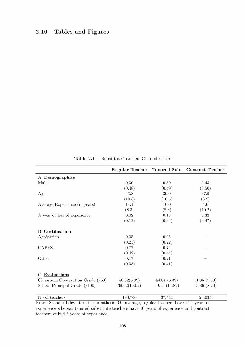
2.10 Tables and Figures

Table 2.1 – Substitute Teachers Characteristics

Regular Teacher Tenured Sub. Contract Teacher

A. Demographics

Male 0.36 0.39 0.43(0.48) (0.49) (0.50)

Age 43.8 39.0 37.9(10.3) (10.5) (8.9)

Average Experience (in years) 14.1 10.0 4.6(8.3) (8.8) (10.2)

A year or less of experience 0.02 0.13 0.32(0.12) (0.34) (0.47)

B. CertificationAgregation 0.05 0.05 –

(0.23) (0.22)CAPES 0.77 0.74 –

(0.42) (0.44)Other 0.17 0.21 –

(0.38) (0.41)

C. EvaluationsClassroom Observation Grade (/60) 46.82(5.99) 44.84 (6.39) 11.85 (9.59)School Principal Grade (/100) 39.02(10.05) 39.15 (11.82) 13.86 (8.70)

Nb of teachers 193,766 67,541 23,035Note : Standard deviation in parenthesis. On average, regular teachers have 14.1 years ofexperience whereas tenured substitute teachers have 10 years of experience and contractteachers only 4.6 years of experience.

108

Table 2.2 – Effect of Absence and Replaced Days on Student Test Scores in 9thGrade

in % of a SD (1) (2) (3)

# days of absence -0.130*** -0.044*** -0.028***(0.009) (0.006) (0.005)

# replaced days 0.056*** 0.010* 0.010*(0.011) (0.006) (0.006)

Av. nb of days of abs. [13.14] [13.14] [13.14]Av. nb of replaced days [10.06] [10.06] [10.06]

Teacher-School Fixed effect No Yes YesTeacher experience & seniority* No Yes YesClassroom Fixed Effects No No Yes

Number of observations 32,290,084 32,290,084 32,290,084

* Quadratic function of teacher experience and of teacher seniority. Each column corres-ponds to a single regression. Results are reported in percentage of a standard deviation.All regressions include year x subject fixed effects. Robust standard errors clustered byschool.Note : With teacher-school fixed effects, teacher experience and seniority and studentbackground as controls (column 3), the marginal impact of one day of absence is toreduce student test score by 0.04 % of a standard deviation. The coefficient is statisticallysignificant at the 1 % level. The number of replaced days does not have any statisticallysignificant impact on student test scores.

109

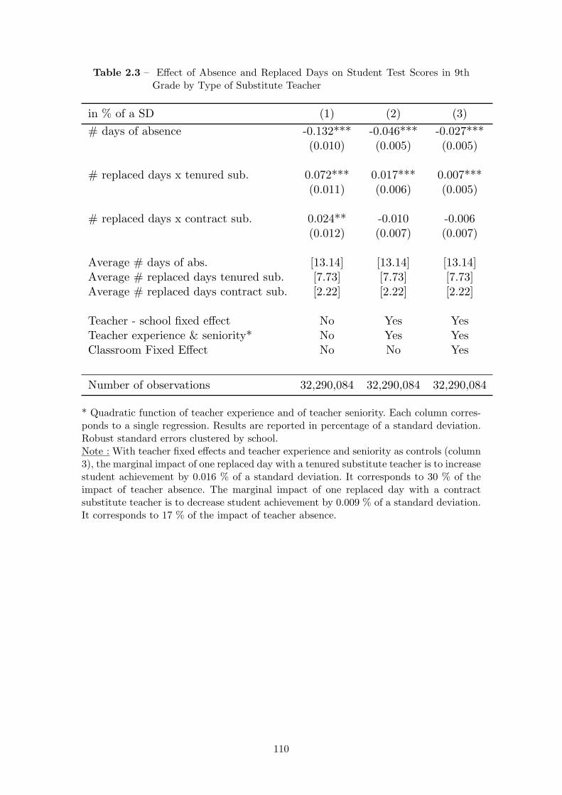
Table 2.3 – Effect of Absence and Replaced Days on Student Test Scores in 9thGrade by Type of Substitute Teacher

in % of a SD (1) (2) (3)

# days of absence -0.132*** -0.046*** -0.027***(0.010) (0.005) (0.005)

# replaced days x tenured sub. 0.072*** 0.017*** 0.007***(0.011) (0.006) (0.005)

# replaced days x contract sub. 0.024** -0.010 -0.006(0.012) (0.007) (0.007)

Average # days of abs. [13.14] [13.14] [13.14]Average # replaced days tenured sub. [7.73] [7.73] [7.73]Average # replaced days contract sub. [2.22] [2.22] [2.22]

Teacher - school fixed effect No Yes YesTeacher experience & seniority* No Yes YesClassroom Fixed Effect No No Yes

Number of observations 32,290,084 32,290,084 32,290,084

* Quadratic function of teacher experience and of teacher seniority. Each column corres-ponds to a single regression. Results are reported in percentage of a standard deviation.Robust standard errors clustered by school.Note : With teacher fixed effects and teacher experience and seniority as controls (column3), the marginal impact of one replaced day with a tenured substitute teacher is to increasestudent achievement by 0.016 % of a standard deviation. It corresponds to 30 % of theimpact of teacher absence. The marginal impact of one replaced day with a contractsubstitute teacher is to decrease student achievement by 0.009 % of a standard deviation.It corresponds to 17 % of the impact of teacher absence.

110

Table 2.4 – Impact of days of absence/replacement in 9th Grade by ExperienceGap between Regular and Substitute Teacher

in % of a SD of student test scores

# days of absence -0.039***(0.005)

# replaced days x tenured sub. 0.015**(0.008)

# replaced days x tenured sub. x exp. gap regular-tenured sub. -0.000(0.000)

# replaced days x contract sub. 0.014(0.013)

# replaced days x contract sub. x exp. gap regular-contract sub. - 0.001**(0.000)

Average # days of abs. [13.14]Average # replaced days tenured sub. [7.73]Average # replaced days contract sub. [2.22]

Teacher - school and classroom fixed effect YesTeacher experience & seniority YesStudent background Yes

Number of observations 32,290,084Robust standard errors clustered by school.

111

Figure 2.1 – Distribution of Absence Spells by Teacher-Year

Note : 55 % of secondary teachers do not take any absence spell per year.

112

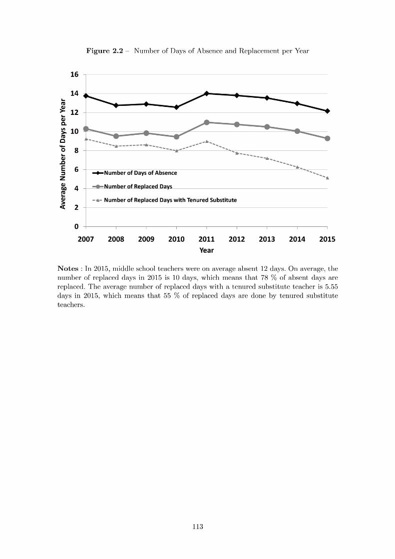
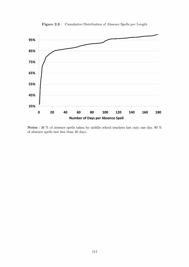
Figure 2.4 – Replacement Rate per Length of Absence Spell

0.2

.4.6

.81

Repla

cem

ent

Rate

1 21 41 61 81 101 121 141 161 181Number of days per absence spells

All Contract Teacher

Notes : 70 % of absence spells lasting 40 days are replaced (black line). 10 % of absencespells lasting 40 days are replaced by a contract substitute teacher. This implies that 60 %of 40 days absence spells are replaced by a tenured substitute teacher.

115

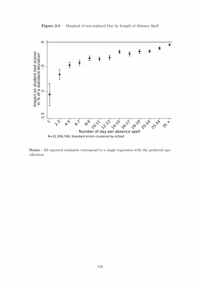
Figure 2.5 – Marginal of non-replaced Day by Length of Absence Spell

-1.5

-1-.

50

Impact

on s

tudent

test

sco

res

in %

of

a s

tandard

devia

tion

12-

34-

56-

78-

9

10-1

1

12-1

3

14-1

5

16-1

7

18-1

9

20-2

4

25-3

435

+

Number of day per absence spellN=32,206,706; Standard errors clustered by school

Notes : All reported estimates correspond to a single regression with the preferred spe-cification.

116

Figure 2.6 – Impact of Absence/Replacement by Teaching subject

-.1

-.0

8-.

06

-.0

4-.

02

0

Impact

on s

tudent

test

sco

res

in %

of

a s

tandard

devia

tion

Math French History

Non replaced day Replaced day with contract sub.Replaced day with tenured sub.

Standard errors clustered by school

Notes : Estimates by subject are estimated through interaction terms. For each subject,the first reported estimates corresponds to the number of days of non-replaced absence,the second to the number of days with a contract teacher and the third to the number ofdays with a tenured substitute teacher. The marginal impact of one day of non-replacedabsence of the Math teacher is to reduce student test scores by 0.86 % of a standarddeviation. This impact is statistically significant at the five percent level.

117

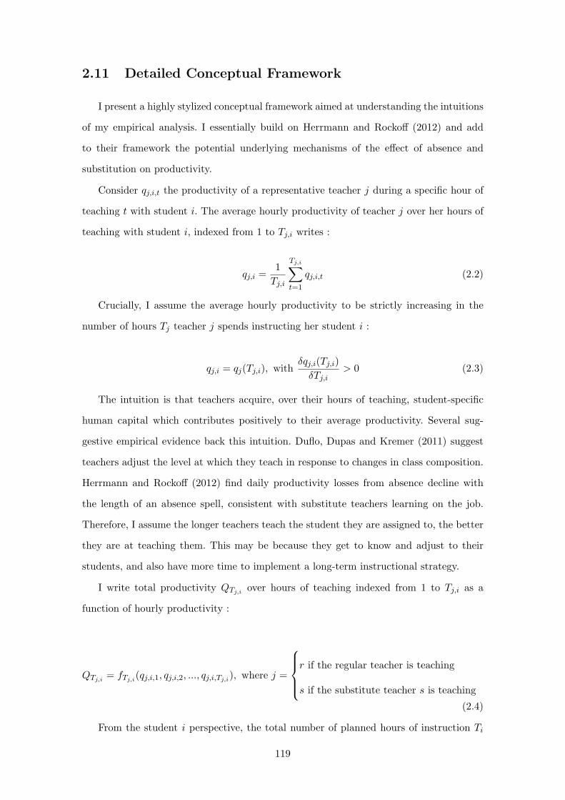
2.11 Detailed Conceptual Framework

I present a highly stylized conceptual framework aimed at understanding the intuitions

of my empirical analysis. I essentially build on Herrmann and Rockoff (2012) and add

to their framework the potential underlying mechanisms of the effect of absence and

substitution on productivity.

Consider qj,i,t the productivity of a representative teacher j during a specific hour of

teaching t with student i. The average hourly productivity of teacher j over her hours of

teaching with student i, indexed from 1 to Tj,i writes :

qj,i =1

Tj,i

Tj,i∑

t=1

qj,i,t (2.2)

Crucially, I assume the average hourly productivity to be strictly increasing in the

number of hours Tj teacher j spends instructing her student i :

qj,i = qj(Tj,i), withδqj,i(Tj,i)

δTj,i> 0 (2.3)

The intuition is that teachers acquire, over their hours of teaching, student-specific

human capital which contributes positively to their average productivity. Several sug-

gestive empirical evidence back this intuition. Duflo, Dupas and Kremer (2011) suggest

teachers adjust the level at which they teach in response to changes in class composition.

Herrmann and Rockoff (2012) find daily productivity losses from absence decline with

the length of an absence spell, consistent with substitute teachers learning on the job.

Therefore, I assume the longer teachers teach the student they are assigned to, the better

they are at teaching them. This may be because they get to know and adjust to their

students, and also have more time to implement a long-term instructional strategy.

I write total productivity QTj,iover hours of teaching indexed from 1 to Tj,i as a

function of hourly productivity :

QTj,i= fTj,i

(qj,i,1, qj,i,2, ..., qj,i,Tj,i), where j =

r if the regular teacher is teaching

s if the substitute teacher s is teaching

(2.4)

From the student i perspective, the total number of planned hours of instruction Ti

119

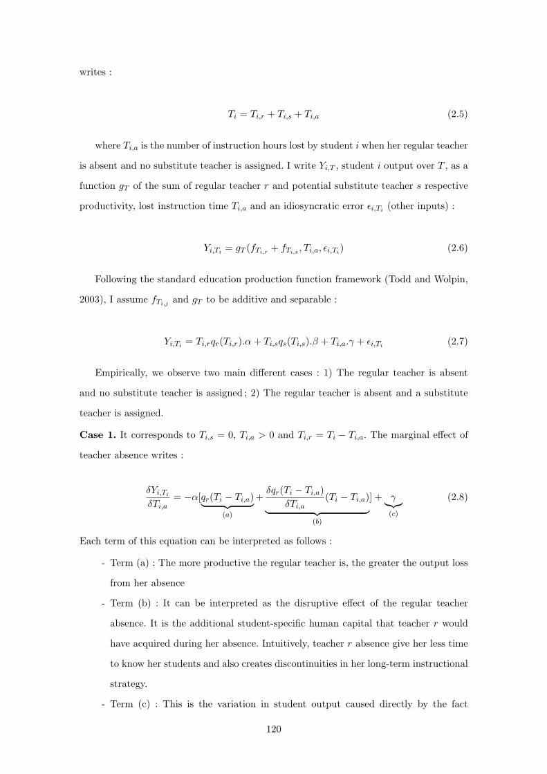
writes :

Ti = Ti,r + Ti,s + Ti,a (2.5)

where Ti,a is the number of instruction hours lost by student i when her regular teacher

is absent and no substitute teacher is assigned. I write Yi,T , student i output over T , as a

function gT of the sum of regular teacher r and potential substitute teacher s respective

productivity, lost instruction time Ti,a and an idiosyncratic error ǫi,Ti(other inputs) :

Yi,Ti= gT (fTi,r

+ fTi,s, Ti,a, ǫi,Ti

) (2.6)

Following the standard education production function framework (Todd and Wolpin,

2003), I assume fTi,jand gT to be additive and separable :

Yi,Ti= Ti,rqr(Ti,r).α+ Ti,sqs(Ti,s).β + Ti,a.γ + ǫi,Ti

(2.7)

Empirically, we observe two main different cases : 1) The regular teacher is absent

and no substitute teacher is assigned ; 2) The regular teacher is absent and a substitute

teacher is assigned.

Case 1. It corresponds to Ti,s = 0, Ti,a > 0 and Ti,r = Ti − Ti,a. The marginal effect of

teacher absence writes :

δYi,Ti

δTi,a= −α[qr(Ti − Ti,a)

︸ ︷︷ ︸

(a)

+δqr(Ti − Ti,a)

δTi,a(Ti − Ti,a)

︸ ︷︷ ︸

(b)

] + γ︸︷︷︸

(c)

(2.8)

Each term of this equation can be interpreted as follows :

- Term (a) : The more productive the regular teacher is, the greater the output loss

from her absence

- Term (b) : It can be interpreted as the disruptive effect of the regular teacher

absence. It is the additional student-specific human capital that teacher r would

have acquired during her absence. Intuitively, teacher r absence give her less time

to know her students and also creates discontinuities in her long-term instructional

strategy.

- Term (c) : This is the variation in student output caused directly by the fact

120

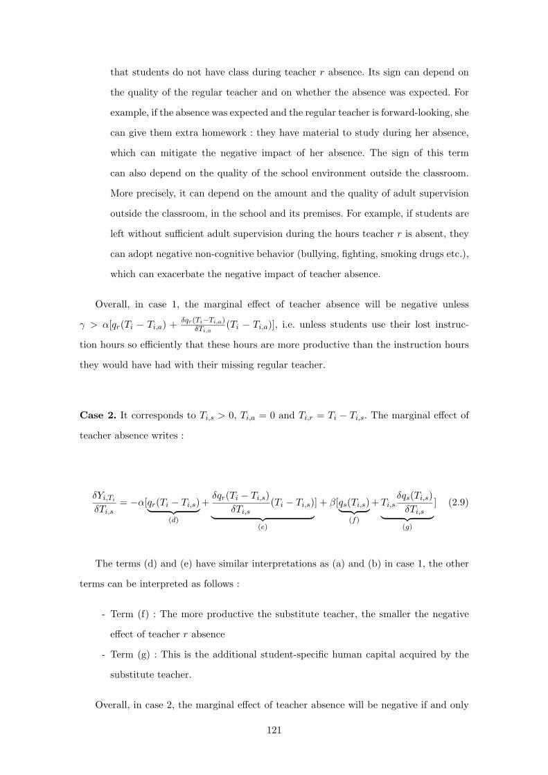
that students do not have class during teacher r absence. Its sign can depend on

the quality of the regular teacher and on whether the absence was expected. For

example, if the absence was expected and the regular teacher is forward-looking, she

can give them extra homework : they have material to study during her absence,

which can mitigate the negative impact of her absence. The sign of this term

can also depend on the quality of the school environment outside the classroom.

More precisely, it can depend on the amount and the quality of adult supervision

outside the classroom, in the school and its premises. For example, if students are

left without sufficient adult supervision during the hours teacher r is absent, they

can adopt negative non-cognitive behavior (bullying, fighting, smoking drugs etc.),

which can exacerbate the negative impact of teacher absence.

Overall, in case 1, the marginal effect of teacher absence will be negative unless

γ > α[qr(Ti − Ti,a) +δqr(Ti−Ti,a)

δTi,a(Ti − Ti,a)], i.e. unless students use their lost instruc-

tion hours so efficiently that these hours are more productive than the instruction hours

they would have had with their missing regular teacher.

Case 2. It corresponds to Ti,s > 0, Ti,a = 0 and Ti,r = Ti − Ti,s. The marginal effect of

teacher absence writes :

δYi,Ti

δTi,s= −α[qr(Ti − Ti,s)

︸ ︷︷ ︸

(d)

+δqr(Ti − Ti,s)

δTi,s(Ti − Ti,s)

︸ ︷︷ ︸

(e)

] + β[qs(Ti,s)︸ ︷︷ ︸

(f)

+Ti,sδqs(Ti,s)

δTi,s︸ ︷︷ ︸

(g)

] (2.9)

The terms (d) and (e) have similar interpretations as (a) and (b) in case 1, the other

terms can be interpreted as follows :

- Term (f) : The more productive the substitute teacher, the smaller the negative

effect of teacher r absence

- Term (g) : This is the additional student-specific human capital acquired by the

substitute teacher.

Overall, in case 2, the marginal effect of teacher absence will be negative if and only

121

if :

α[qr(Ti − Ti,s) +δqr(Ti − Ti,s)

δTi,s(Ti − Ti,s)] > β[qs(Ti,s) + Ti,s

δqs(Ti,s)

δTi,s] (2.10)

In particular, equation (2.10) will be verified when the regular teacher is of higher

quality than the substitute teacher (qr > qs) and/or when the regular teacher acquire

student-specific human capital faster than the substitute teacher ( δqr/δTi,r > δqs/δTi,s).

Table 2.5 – Performance at the Certification Exam of the Contract Teachers whotake it

Contract Teachers Candidates Other Candidates

Agreg. CAPES Agreg. CAPES

A. Demographics

Age (in years) 37.72 35.17 31.05 28.18(7.75) (7.68) (8.32) (6.65)

Male 0.53 0.39 0.46 0.35(0.50) (0.48) (0.49) (0.48)

B. PerformancePassing Rate 0.03 0.16 0.15 0.33

(0.18) (0.37) (0.36) (0.47)Written Part Grade (/20) 3.91 5.67 6.25 7.30

(2.52) (3.14) (3.61) (3.69)Oral Part Grade (/20) 7.00 7.30 8.09 8.50

(3.78) (4.17) (3.83) (4.58)

Nb of obs 286 1,232 8,037 11,779

Note : Standard deviation in parenthesis. On average, the passing rate of contract teachersat the CAPES examination is 16 %. The average passing rate of other candidates is 33 %.

122

Table 2.6 – Regression Estimates of the Relationship between Ab-sence/Replacement and Teacher Characteristics

# Abs. Days Share Replaced Days Share Replaced x Contr. Share Replaced x Tenured Sub.(1) (2) (3) (4) (5) (6) (7) (8)

Experience (Ref : 6 + years)

One year or less of experience -4.976∗∗∗ -4.099 -0.043∗∗∗ -0.056∗∗∗ -0.012∗∗ -0.014 -0.031∗∗∗ -0.045∗∗∗

(1.255) (2.479) (0.008) (0.016) (0.005) (0.009) (0.006) (0.011)

Two years of experience -4.854∗∗∗ -5.415∗∗∗ -0.026∗∗∗ -0.0382∗∗∗ -0.008∗∗ -0.017∗∗∗ -0.018∗∗∗ -0.020∗∗

(0.613) (1.061) (0.005) (0.008) (0.002) (0.005) (0.004) (0.007)

Three years of experience -3.475∗∗∗ -4.059∗∗∗ -0.019∗∗∗ -0.025∗∗∗ -0.005∗ -0.011∗∗∗ -0.013∗∗∗ -0.0138∗∗

(0.455) (0.658) (0.004) (0.006) (0.002) (0.003) (0.003) (0.005)

Four years of experience -1.706∗∗∗ -2.711∗∗∗ -0.006∗ -0.012∗∗ -0.000 -0.006∗ -0.006∗ -0.007(0.377) (0.532) (0.003) (0.004) (0.002) (0.003) (0.002) (0.004)

Five years of experience 0.637 -0.681 0.008∗∗ 0.000 0.007∗∗∗ 0.000 0.001 0.000(0.350) (0.449) (0.002) (0.003) (0.001) (0.002) (0.002) (0.003)

Seniority (Ref. : 6 + years)

One year of seniority 5.320 22.930 0.498∗∗ 0.649∗∗ 0.332 0.294 0.167 0.356(10.26) (13.150) (0.210) (0.257) (0.200) (0.263) (0.177) (0.319)

Two years of seniority 3.084∗∗∗ 0.004 0.018∗∗∗ 0.004 0.007∗∗∗ -0.002 0.012∗∗∗ 0.006∗

(0.268) (0.437) (0.001) (0.003) (0.001) (0.002) (0.001) (0.003)

Three years of seniority 1.545∗∗∗ 1.001∗∗ 0.012∗∗∗ 0.0111∗∗∗ 0.005∗∗∗ 0.002 0.008∗∗∗ 0.009∗∗∗

(0.223) (0.365) (0.00171) (0.002) (0.000) (0.001) (0.001) (0.002)

Four years of seniority 1.368∗∗∗ 1.112∗∗∗ 0.011∗∗∗ 0.0101∗∗∗ 0.005∗∗∗ 0.002 0.006∗∗∗ 0.007∗∗∗

(0.222) (0.315) (0.001) (0.002) (0.000) (0.001) (0.001) (0.002)

Five years of seniority 0.695∗∗∗ 0.374 0.007∗∗∗ 0.004∗∗ 0.004∗∗∗ 0.001 0.003∗∗∗ 0.003(0.205) (0.275) (0.001) (0.002) (0.000) (0.001) (0.001) (0.001)

EvaluationsClassrom Obs. Eval. -0.266∗∗∗ 0.0115 -0.001∗∗∗ 0.000 -0.000 -0.000 -0.000 0.000

(0.0170) (0.0371) (0.000) (0.000) (0.000) (0.000) (0.000) (0.000)

School Principal Eval. -0.532∗∗∗ -0.222∗∗∗ -0.004∗∗∗ -0.002∗∗∗ -0.001∗∗∗ -0.000 -0.003∗∗∗ -0.002∗∗

(0.065) (0.075) (0.000) (0.000) (0.000) (0.000) (0.000) (0.000)

Student Composition

Prop. of financial aid students -0.492* 0.901* -0.007∗∗∗ 0.002 0.003∗∗∗ 0.001 -0.009∗∗∗ 0.001(0.339) (0.530) (0.002) (0.006) (0.001) (0.002) (0.001) (0.005)

GenderMale -4.688∗∗∗ -0.029∗∗∗ -0.013∗∗∗ -0.017∗∗∗

(0.124) (0.000) (0.000) (0.000)

Certification Level (Ref : Capes)

Agregation 0.383 0.003 0.002∗ 0.001(0.219) (0.002) (0.000) (0.001)

Teaching subject (Ref. : History)

French 0.855∗∗∗ -0.002∗ 0.002∗∗∗ -0.003∗∗∗

(0.158) (0.001) (0.0005) (0.002)

Math -0.851∗∗∗ -0.002∗∗ 0.007∗∗∗ -0.010∗∗∗

(0.144) (0.001) (0.000) (0.000)

Teacher - school fixed effects No Yes No Yes No Yes No YesNb. of obs. 282,001 282,001 282,001 282,001 282,001 282,001 282,001 282,001

* Each column corresponds to a single regression. Results are reported in percentage ofa standard deviation. All regressions include year fixed effects. Robust standard errorsclustered by teacher-school.Note : With teacher-school fixed effects, the relationship between the share of financialaid students assigned to a teacher and her share of replaced absent days is negative andstatistically significant at the 1 % level.

123

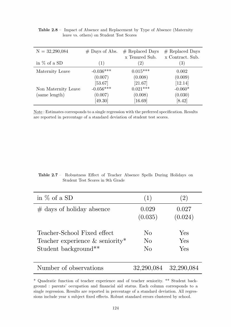
Table 2.8 – Impact of Absence and Replacement by Type of Absence (Maternityleave vs. others) on Student Test Scores

N = 32,290,084 # Days of Abs. # Replaced Days # Replaced Daysx Tenured Sub. x Contract. Sub.

in % of a SD (1) (2) (3)

Maternity Leave -0.036*** 0.015*** 0.002(0.007) (0.008) (0.009)[53.67] [21.67] [12.14]

Non Maternity Leave -0.056*** 0.021*** -0.060*(same length) (0.007) (0.008) (0.030)

[49.30] [16.69] [8.42]

Note : Estimates corresponds to a single regression with the preferred specification. Resultsare reported in percentage of a standard deviation of student test scores.

Table 2.7 – Robustness Effect of Teacher Absence Spells During Holidays onStudent Test Scores in 9th Grade

in % of a SD (1) (2)

# days of holiday absence 0.029 0.027(0.035) (0.024)

Teacher-School Fixed effect No YesTeacher experience & seniority* No YesStudent background** No Yes

Number of observations 32,290,084 32,290,084

* Quadratic function of teacher experience and of teacher seniority. ** Student back-ground : parents’ occupation and financial aid status. Each column corresponds to asingle regression. Results are reported in percentage of a standard deviation. All regres-sions include year x subject fixed effects. Robust standard errors clustered by school.

124

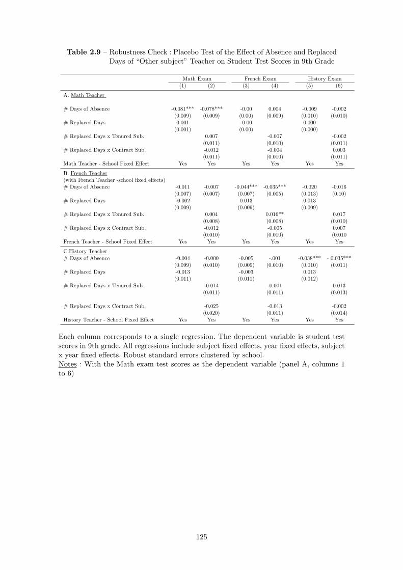
Table 2.9 – Robustness Check : Placebo Test of the Effect of Absence and ReplacedDays of “Other subject” Teacher on Student Test Scores in 9th Grade

Math Exam French Exam History Exam(1) (2) (3) (4) (5) (6)

A. Math Teacher

# Days of Absence -0.081*** -0.078*** -0.00 0.004 -0.009 -0.002(0.009) (0.009) (0.00) (0.009) (0.010) (0.010)

# Replaced Days 0.001 -0.00 0.000(0.001) (0.00) (0.000)

# Replaced Days x Tenured Sub. 0.007 -0.007 -0.002(0.011) (0.010) (0.011)

# Replaced Days x Contract Sub. -0.012 -0.004 0.003(0.011) (0.010) (0.011)

Math Teacher - School Fixed Effect Yes Yes Yes Yes Yes Yes

B. French Teacher(with French Teacher -school fixed effects)# Days of Absence -0.011 -0.007 -0.044*** -0.035*** -0.020 -0.016

(0.007) (0.007) (0.007) (0.005) (0.013) (0.10)# Replaced Days -0.002 0.013 0.013

(0.009) (0.009) (0.009)# Replaced Days x Tenured Sub. 0.004 0.016** 0.017

(0.008) (0.008) (0.010)# Replaced Days x Contract Sub. -0.012 -0.005 0.007

(0.010) (0.010) (0.010French Teacher - School Fixed Effect Yes Yes Yes Yes Yes Yes

C.History Teacher

# Days of Absence -0.004 -0.000 -0.005 -.001 -0.038*** - 0.035***(0.099) (0.010) (0.009) (0.010) (0.010) (0.011)

# Replaced Days -0.013 -0.003 0.013(0.011) (0.011) (0.012)

# Replaced Days x Tenured Sub. -0.014 -0.001 0.013(0.011) (0.011) (0.013)

# Replaced Days x Contract Sub. -0.025 -0.013 -0.002(0.020) (0.011) (0.014)

History Teacher - School Fixed Effect Yes Yes Yes Yes Yes Yes

Each column corresponds to a single regression. The dependent variable is student testscores in 9th grade. All regressions include subject fixed effects, year fixed effects, subjectx year fixed effects. Robust standard errors clustered by school.Notes : With the Math exam test scores as the dependent variable (panel A, columns 1to 6)

125

Table 2.10 – Robustness Check : Placebo Test of the Effect of Absence and Repla-ced Days of Previous and Following Year on Student Test Scores in9th Grade

Previous year Following year(1) (2) (3) (4)

# Days of Absence 0.004 0.003 0.002 0.000(0.019) (0.020) (0.013) (0.013)

# Replaced Days 0.015 0.004(0.023) (0.018)

# Replaced Days x Tenured Sub. 0.023 0.003(0.027) (0.020)

# Replaced Days x Contract Sub. 0.008 0.018(0.029) (0.027)

Teacher - school fixed effect No No Yes YesTeacher experience & seniority* Yes Yes Yes YesClassroom Fixed Effect Yes Yes Yes YesNumber of observations 31,643,528 31,643,528 31,643,528 31,643,528

* Quadratic function of teacher experience and of teacher seniority. ** Student back-ground : parents’ occupation and financial aid status. Each column corresponds to asingle regression. Results are reported in percentage of a standard deviation. The levelof observation is teacher/topic x student x year. All regressions include year x subjectfixed effects. Robust standard errors clustered by teacher-school. Robust standard errorsclustered by school.Notes : In columns 1 and 2, the number of days of absence, number of replaced daysand number of replaced days with the two types of substitute teachers of the previousyear are used as independent variables. Column 1 shows that the marginal impact of oneadditional day of absence and replacement of the teacher in the year n− 1 does not haveany statistically significant impact on her student test scores, assigned to her during theyear n.

126

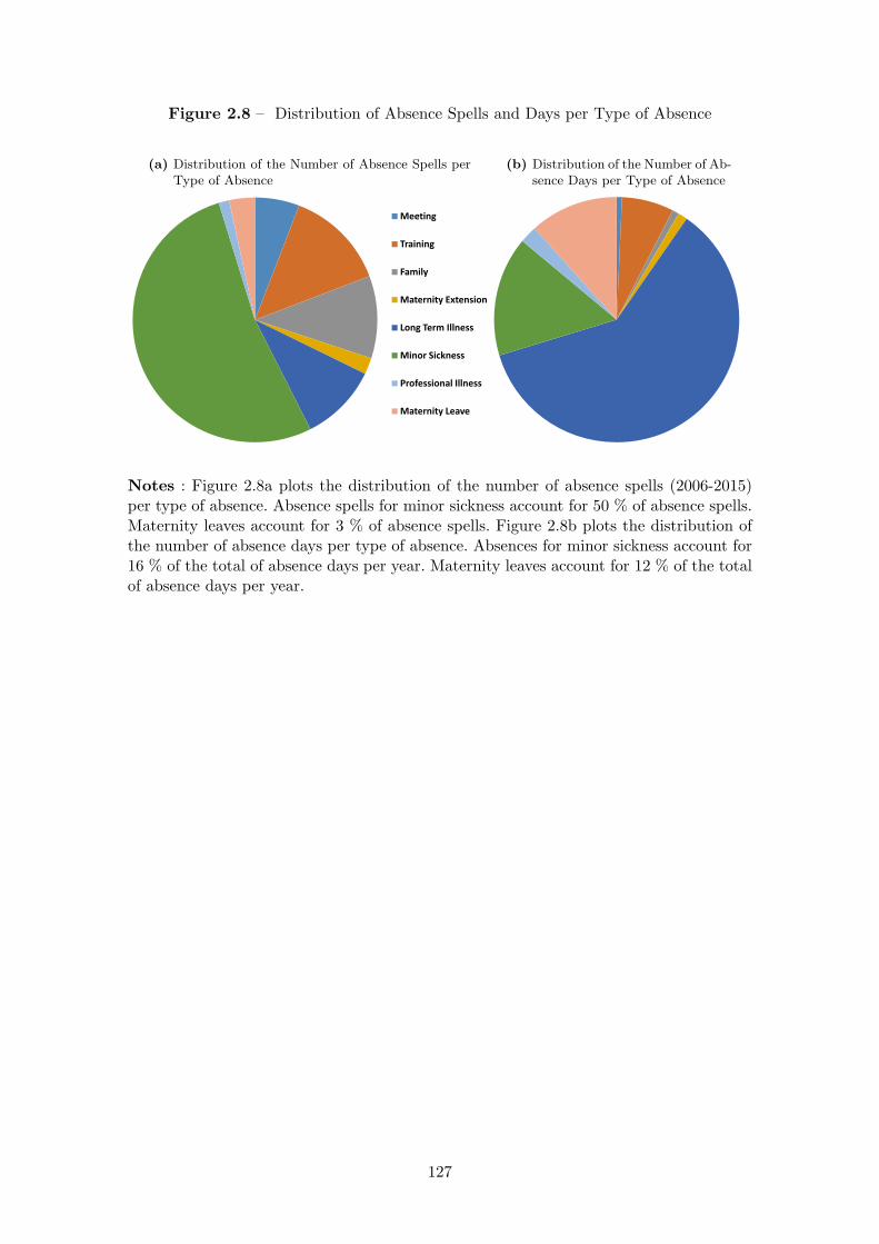
Figure 2.8 – Distribution of Absence Spells and Days per Type of Absence

(a) Distribution of the Number of Absence Spells perType of Absence

Meeting

Training

Family

Maternity Extension

Long Term Illness

Minor Sickness

Professional Illness

Maternity Leave

(b) Distribution of the Number of Ab-sence Days per Type of Absence

Notes : Figure 2.8a plots the distribution of the number of absence spells (2006-2015)per type of absence. Absence spells for minor sickness account for 50 % of absence spells.Maternity leaves account for 3 % of absence spells. Figure 2.8b plots the distribution ofthe number of absence days per type of absence. Absences for minor sickness account for16 % of the total of absence days per year. Maternity leaves account for 12 % of the totalof absence days per year.

127

The OCC and CONG datasets are raw administrative datasets which are not pre-

viously cleaned by the Statistical Department of the Ministry of Education. I do not use

the cleaned version of these datasets because they are not exhaustive :

1. The cleaned version of the OCC datasets does not include all teacher assignment

spells but only the assignment spells which are ongoing at the time of the ex-

traction by the Statistical Department (in December of each year). This is highly

problematic for the purpose of this study because I need to observe all teacher assi-

gnments through the school year in order to know, for each absence spell, whether

a substitute teacher has been assigned, and the identity of this substitute teacher.

2. The cleaned version of the CONG datasets does not include all teacher absence

spells but only absence for heath reasons : minor sickness, maternity leave, long

term illness and professional illness. This is highly problematic because, as shown

in figure 2.8b, non health related absences (meetings, training, family) represent

around 30 % of absence spells.

129

130

Chapitre 3

Stay a Little Longer ? Teacher

Turnover, Retention and Quality

in Disadvantaged Schools

Using French administrative data on secondary school teachers, we analyze a non-

pecuniary, “career-path oriented” centralized incentive scheme designed to attract and

retain teachers in French disadvantaged schools. We rely on a major reform of the struc-

ture of this incentive scheme to identify its effect on teacher turnover, retention, and

quality in disadvantaged schools. We find this incentive scheme has a statistically signi-

ficant positive effect on the number of consecutive years teachers stay in disadvantaged

schools and decreases the probability of inexperienced teachers in disadvantaged schools

to leave the profession. However, we find no statistically significant effect on the teacher

experience gap nor the student achievement gap between disadvantaged and non disad-

vantaged schools.

Keywords : teachers, teacher mobility, teacher retention, educational inequalities, edu-

cation prioritaire. JEL : I21, I22, J20.

3.1 Introduction

In many countries, disadvantaged students are more likely to be assigned to lower

quality teachers (OECD, 2005). In the United States for example, disadvantaged students

are 10 percent more likely to be taught by teachers in the bottom 10 percent of the

131

teacher quality distribution than non disadvantaged students (Goldhaber et al., 2015).

The magnitude of this teacher quality gap in the US is equivalent to 20 percent of the

student achievement gap (Darling-Hammond, 2015). There is a large literature showing

that teacher quality matters for student outcomes (Rockoff, 2004 ; Chetty et al., 2014).

Reducing the teacher quality gap is therefore a major policy issue in order to provide

more equal educational opportunity.

There are very few papers analysing policies aiming at reducing the teacher quality

gap. The main type of policies studied are financial bonus schemes for teachers working

in disadvantaged schools. This literature remains inconclusive (Clotfelter et al., 2008 ;

Prost, 2013). Furthermore, there is strong evidence showing that teachers do care about

non-pecuniary factors (Hanushek et al., 2004).

This paper analyzes a “career-path oriented” centralized incentive scheme designed to

reduce the teacher quality gap between disadvantaged and non-disadvanged public middle

schools in France. To our best knowledge, there is no existing empirical evidence on the

impact of teachers’ non-pecuniary incentives on the teacher quality gap.

In France, teachers are assigned according to a centralized point-based assignment

system. Teachers submit a ranked-ordered list of choices and are assigned according to

a modified version of the deferred acceptance mechanism. The main assignment criteria

are i) experience, defined as the number of years since entering the teaching profession ;

ii) seniority, defined as the number of consecutive years spent in the current school ; iii)

seniority in the same disadvantaged school.

This paper evaluates the last criteria : how effective is the disadvantaged school senio-

rity bonus at attracting and retaining quality teachers in disadvantaged schools ? What

is its effect on the student achievement gap in middle school ? In order to assess this

scheme, we exploit a major reform in 2005 which changed i) the set of disadvantaged

schools benefiting from this extra seniority bonus ; ii) the structure of this bonus. This

change in structure aims at giving teachers the incentives to stay at least five consecutive

years in the same disadvantaged school, instead of three consecutive years before the re-

form. This paper relies on comprehensive administrative data on middle school teachers

and students from 2002 to 2014 to perform a difference-in-difference comparing the evo-

lution of the disadvantaged schools receiving the bonus to the other schools before/after

the 2005 reform. Disadvantaged schools benefitting from extra seniority points before the

132

reform are part of the Zone d’Education Prioritaire, violent schools or sensitive schools

programs (19 % of middle schools), hereafter called ZEP schools for simplicity. Disadvan-

taged schools benefiting from extra seniority points ( 13 % of middle schools) after the

reform are called Affectation prioritaire a valoriser, hereafter APV. We analyze the impact

of the 2005 reform on several outcomes at the school level : teacher turnover, measured

by teacher mobility rate and seniority ; teacher quality, measured by teacher experience ;

student achievement, measured by their test scores at the national standardized exam

Diplome national du brevet (DNB) taken in 9th grade.

We find that the reform has a positive impact on teacher seniority in APV schools.

The reform provokes a progressive decrease in the seniority gap between APV and non-

APV schools reaching 20 % (0.3 years) at the end of the period. We also find that the

reform decreases the probability of inexperienced teachers (i.e. with less than 10 years

of teaching experience) in APV school to leave the teaching profession. Finally, we find

that the reform has no statistically significant impact on the quality of teachers moving

to APV schools, as measured by their number of years of experience, nor on the student

achievement gap between APV and non-APV schools.

3.2 Institutional Setting

We present the main features of the French educational system as well as the 2005

reform of the disadvantaged school mobility bonus.

3.2.1 Overview of the French Educational System

The public French educational system is highly centralized. Contrary to the United

States for example, schools have little autonomy and school principals cannot hire nor fire

their teachers. The French territory is composed of 25 large administrative school districts,

called academies (hereafter regions). Secondary school teachers are selected through a

subject-specific national competitive examination, which is demanding academically and

has low passing rates (between 15 and 30 %). There are two main certification levels :

basic, called CAPES (Certificat d’aptitude au professorat de l’enseignement du second

degre) and advanced, called Agregation. Conditional on passing this examination, teachers

become civil servants managed by their region.

133

Teachers’s salary is set through a national wage scale based on teachers’ number of

years of experience and certification level (none, basic and advanced). For example, the

gross wage of a teacher with the basic certification level and a year of experience is

approximately 2,000 euros per month. Contrary to other countries such as the United

States for example, wages do not vary across schools.

Teachers can however receive a small financial compensation for teaching in the disad-

vantaged schools that are part of the Zone d’education prioritaire (ZEP) program (Prost,

2013). The ZEP program, established in 1982, is a compensatory education policy giving

additional resources (smaller class size, etc.) to a selected set of disadvantaged schools.

ZEP schools are selected by the central government according to the socioeconomic back-

ground of their students. The ZEP financial compensation was introduced in 1990 at 300

euros per year, and was continuously increased to reach 1,156 euros per year in 2010.

Secondary school teachers are subject-specific : each subject is taught by a different

teacher. In middle school (from grade 6 to grade 9), students are not tracked by major

nor ability. Contrary to many countries such as the United States where students’ peers

depend on the teaching subject, in France, students stay in the same class, with the same

peers throughout the school year and in every subject. At the end of 9th grade, students

take a national and externally graded examination called Diplome national du Brevet in

three topics : French, Math and History.

3.2.2 Certified Teacher Assignment and the 2005 Reform

Certified Secondary School Teacher Assignment. In many countries such as the

United States for example, teachers are hired directly by schools. In France, secondary

school certified teachers are assigned via a centralized point-based system (called SIAM,

Systeme d’information et d’aide aux mutations) with two rounds : the inter-regional round

and the regional round. Candidates submit a rank-ordered list of choices and are assigned

according to a modified version of the school-proposing Deferred Acceptance mechanism

(Combes, Tercieux and Terrier, 2017). Every year, i) new teachers and tenured teachers

who want to change region apply to the inter-regional mobility round ; ii) participants of

the inter-regional mobility round, and tenured teachers who want to change school within

their region, apply to the intra-regional mobility round.

Both at the inter and intra regional level, the main assignment criterias are teacher

134

experience (defined as the number of years since entering the teaching profession), senio-

rity (defined as the number of consecutive years spent teaching in the same school) and

seniority in a disadvantaged school.

The 2005 Reform. This reform changed the set of schools benefitting from the extra

seniority bonus. Before 2005, all the schools labelled ZEP benefitted from the additional

seniority bonus. After 2005, a new list of schools, labelled APV (Affectation Prioritaire

justifiant une Valorisation schools) was established. APV schools were selected based on

their lack of attractivity as measured by their teacher turnover rate . The set of APV

schools did not change after 2005. As shown in Table 3.1, most of ZEP schools became

APV schools. However, many ZEP schools did not become APV schools. Therefore, we

create four distinct groups of schools :

- non ZEP and non APV schools (3,920 schools) : the status of these schools did not

change throughout the period

- ZEP and non APV schools (392 schools) : these schools benefitted from the disad-

vantaged school seniority bonus before the reform but not after the reform

- non ZEP an APV schools (140 schools) : these schools did not benefit from the

disadvantanged school seniority bonus before the reform but benefitted from it

after the reform

- ZEP and APV schools (572 schools) : the status of these schools did not change

throughout the period

The 2005 reform also changed the structure of the seniority bonus. Before the 2005

reform, certified teachers got 10 points per year of seniority and 25 additional points

every five years (table 3.3). This seniority bonus does not depend on the status of the

school (ZEP school or not). Teachers assigned to ZEP schools got additional seniority

points depending on their number of years of seniority : 50 additional points for 3 years

of seniority ; 65 points for four years ; 85 points for five years or more.

After the 2005 reform, the structure of the standard seniority bonus changed. Teachers

still get 10 points every year but now they get the additional 25 points every four years

instead of every five years. The structure of the disadvantaged school seniority bonus

also changed. The seniority bonuses at three and four years of seniority were suppressed.

Teachers in APV schools get 300 additional points if they have five to seven years of

seniority, and 400 points if they have 8 years or more of seniority.

135

Figure 3.1 plots the value of the seniority bonus by number of years of seniority,

depending on the status of the school and the period (before or after the 2005 reform).

The reform has a major impact on the disadvantaged school seniority bonus. For example,

before the reform, a certified teacher with five years of seniority in a ZEP school got 4 ×

10 + 85 + 25 = 160 points. After the reform, a similar teacher with five years of seniority

in an APV school gets 4 × 10 + 25 + 300 = 375 points.

The population affected by the reform is composed of teachers assigned to APV schools

from the 2005 onwards but also of teachers who were assigned to ZEP schools before the

reform. A transitory bonus scale was implemented after the reform for teachers who were

assigned to ZEP schools. Table 3.2 shows the transitory scale for the disadvantaged school

seniority bonus. It distinguishes between two types of ZEP schools : ZEP schools which

did not become APV, i.e. schools which stopped benefitting from the extra seniority bonus

after 2005, and ZEP schools that became APV, i.e. schools which continued to benefit

from the bonus after 2005. In both type of schools, the population benefitting from the

transitory scale are teachers assigned to ZEP schools before the 2005 reform. In ZEP &

APV schools, the transitory scale was implemented only in 2005 whereas in ZEP non

APV schools, it was implemented in 2005, 2006 and 2007.

The main motivation of this reform, as stated by the Ministry of Education, is to make

APV schools more attractive for teachers and to reduce teacher turnover. More specifically,

the objective is “to give teachers the incentive to be commited to their assigned APV

schools for at least five years ”.

3.3 Data and Descriptive Evidence

In this section, we briefly present the main characteristics of the data as well descriptive

evidence on the impact of the reform on teacher mobility, seniority and experience in

disadvantaged schools.

3.3.1 Data

This paper relies on comprehensive administrative panel data on teachers, middle

schools and students from the French Ministry of Education :

- Data on teachers and their assignments (2001 - 2014) : this datasets provide in-

136

dividual information on teacher such as their national identifier, their year of as-

signment, their type of assignment (permanent vs. temporary), school identifier,

classroom identifier, number of years of experience, teaching subject

- Data on public secondary schools (2001 - 2014) : national identifier, classification

(ZEP, violent, sensitive), type (middle vs. high schools)

- Secondary school students (2004 - 2014) : encrypted identifier, socio-demographic

characteristics ( financial aid status, profession of both parents), classroom iden-

tifier, test scores at the national and externally graded examination taken in 9th

grade (Diplome national du Brevet)

We did not have access to the dataset from the Ministry of Education listing APV

schools. Thus, we constructed the list of APV schools from the publicly available admi-

nistrative documents on the regions’ official websites.

We are able to match each individual teacher to all her students thanks to the school

and classroom identifiers. Our sample focuses on teachers with a permanent assignment

( 78 % of observations) because temporary teachers are reassigned every year and do not

benefit from the APV bonus. We also focus on public middle schools because there are

almost no APV high schools.

We define the following outcome variables :

- teacher number of years of seniority : number of consecutive years a teacher teaches

in the same school ;

- teacher mobility rate : proportion of teachers leaving their current school for ano-

ther schools. This mobility rate does not include teachers who are leaving the

teaching profession

- teacher exit rate : proportion of teachers who interrupt their teacher career, tem-

porarily (being on a long sabbatical) or permanently (quitting or retiring) . We use

the share of teachers who leave the teacher database as a proxy 1. Each year, bet-

ween three and six percent of teachers leave the teaching profession (Figure 3.15).

This exit rate can have many causes that we do not observe directly in the data.

We have however access to individual teacher retirement data, from 2007 to 2013.

We observe that over this period, teachers in non disasvantaged schools are more

1. As we are using comprehensive administrative datasets, the probability of data collection relatedattrition is negligible

137

likely to retire than other teachers, which is consistent with the difference in the

teacher experience structure between these two types of schools (Figure 3.13 ). In

2007 for example, almost 5% of teachers in non APV and non ZEP schools retired,

against around 2% in APV and ZEP schools. This numbers are consistent with the

descriptive statistics from the Ministry of Education (DEPP, 2014). This suggests

that, in non APV – non ZEP schools, over the 2007-2013, more than 85 % of exits

are due to retirement against less than 50 % in APV and ZEP schools.

Given the objectives of the APV program, we would like to know whether it pro-

vides big enough incentives to deter teachers from quitting the teaching profession.

An established result in the literature in that inexperienced teachers in disadvan-

taged schools are the population the most at risk of quitting (Boyd et al., 2008 ;

Allen et al. 2015). This is why we focus the exit rate analysis to inexperienced tea-

chers, for which the main cause of the exit rate is most likely to be quitting rather

than retiring. To find the specific experience threshold, we plot the retirement rate

by number of years of experience (Figure 3.14) and we observe than teachers with

less than 10 years of experience have a probability close to zero. In the remaining

of the paper, we therefore define inexperienced teachers as having less than ten

years of teaching experience.

- teacher experience : number of years since the teacher entered the teaching profes-

sion

3.3.2 Descriptive Evidence

We provide descriptive evidence on the evolution of teacher mobility, seniority and

experience in the different groups of schools from 2002 to 2015.

Evolution of the Outcome Variables per Year. We first analyse the evolution

of the average teacher mobility rate by school year from 2002 to 2014 ( Figure 3.2). The

mobility rate is much lower in non disadvantaged schools (non ZEP - non APV schools)

than in disadvantaged schools throught the period. The teacher mobility rate in non

disadvantaged schools is around 5 % throughout the period against around 10 % in APV

and ZEP schools. Yet, we do not observe any impact of the reform on the mobility rate

of the different categories of schools.

We now turn to the evolution of the average exit rate of inexperienced teachers (Figure

138

3.3). Overall, the exit rate is slightly lower for inexperienced teachers in non disadvantaged

schools (non ZEP - non APV schools) than in disadvantaged schools, especially APV-ZEP

schools before the reform. This graph seems to suggest that the reform has a negative

impact on the exit rate gap between APV and non APV schools, even though it does not

provide clear causal evidence.

There are also major variations in teacher seniority and experience across the different

groups of schools (Figure 3.4 and Figure 3.5). Teachers in schools both labelled APV and

ZEP have on average, around 8 years of seniority. Teachers in non ZEP - APV schools

have around 9 years of seniority in the begining of the period. However, starting from

2009, their average level of seniority decreases to 8 years, converging with the level of

seniority of teachers in ZEP-APV schools. Teachers in non- disadvantaged schools (non

ZEP - non APV) have on average around 2 more years of seniority, around 10 years of

seniority. Regarding teaching experience, we observe a large gap between disadvantaged

schools ( APV- ZEP, or non ZEP - APV) and non disadvantaged schools (non ZEP - non

APV schools).

Mobility Rate by Number of Years of Seniority. We analyse teacher mobility

by number of years of seniority. We distinguish four periods : i) before the reform : 2002

- 2004 (Figure 3.6) ; ii) year of the reform : 2005 (Figure 3.7) ; iii) transition years : 2006-

2007 (Figure 3.8) ; iv) after the reform : 2008-2014 (Figure 3.9). Vertical lines correspond

to seniority bonuses : black lines indicate seniority bonuses that apply to all types of

schools ; red lines indicate bonuses that apply to ZEP schools before 2005, and to APV

schools after 2005.

Before the reform (2002 - 2004), we observe a spike in the mobility rate at 5 years

of seniority for all types of schools. This spike corresponds to the additional 25 seniority

bonus when teachers reach five years of seniority. For non ZEP- APV schools, the mobility

rate goes from 10 % at four years of seniority to 24 % at five years of seniority. Interestingly,

this is larger than the spike for ZEP schools, which benefit from the extra bonus at 5 years

of seniority (whereas non ZEP - APV schools do not).

In ZEP - APV schools, the mobility rate increases from 3 years of seniority, when

teachers get the 50 points seniority bonus : the mobility rate goes from 8 % at 2 years

of seniority to almost 16 % at 3 years of seniority. This mobility rate remains constant

at 4 years of seniority, when teachers benefit from a 65 points seniority bonus. Finally, it

139

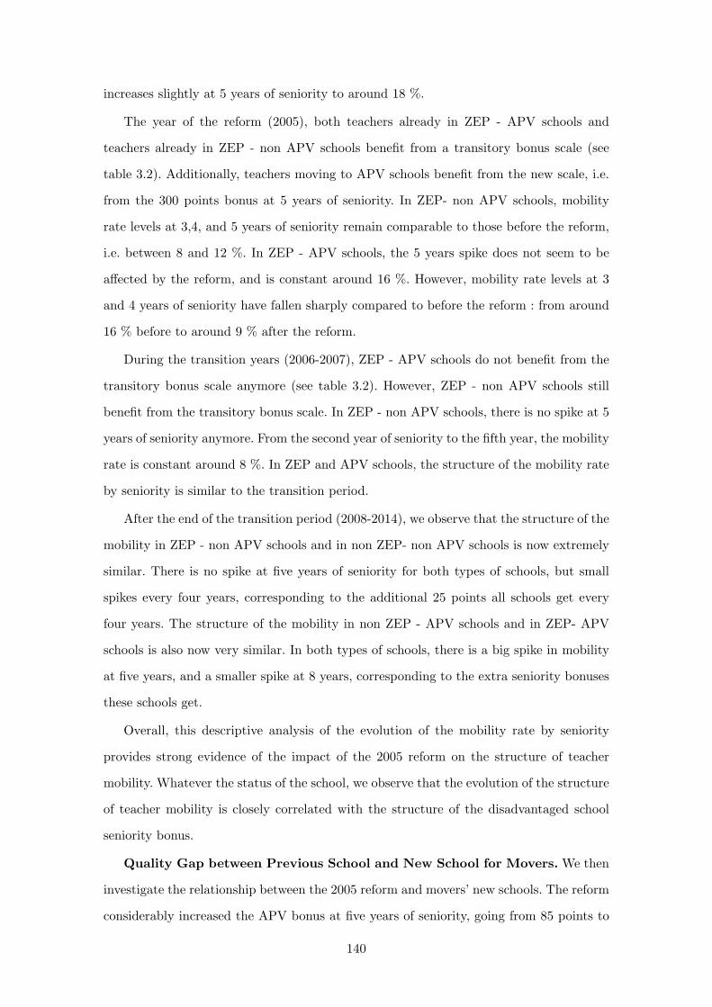
increases slightly at 5 years of seniority to around 18 %.

The year of the reform (2005), both teachers already in ZEP - APV schools and

teachers already in ZEP - non APV schools benefit from a transitory bonus scale (see

table 3.2). Additionally, teachers moving to APV schools benefit from the new scale, i.e.

from the 300 points bonus at 5 years of seniority. In ZEP- non APV schools, mobility

rate levels at 3,4, and 5 years of seniority remain comparable to those before the reform,

i.e. between 8 and 12 %. In ZEP - APV schools, the 5 years spike does not seem to be

affected by the reform, and is constant around 16 %. However, mobility rate levels at 3

and 4 years of seniority have fallen sharply compared to before the reform : from around

16 % before to around 9 % after the reform.

During the transition years (2006-2007), ZEP - APV schools do not benefit from the

transitory bonus scale anymore (see table 3.2). However, ZEP - non APV schools still

benefit from the transitory bonus scale. In ZEP - non APV schools, there is no spike at 5

years of seniority anymore. From the second year of seniority to the fifth year, the mobility

rate is constant around 8 %. In ZEP and APV schools, the structure of the mobility rate

by seniority is similar to the transition period.

After the end of the transition period (2008-2014), we observe that the structure of the

mobility in ZEP - non APV schools and in non ZEP- non APV schools is now extremely

similar. There is no spike at five years of seniority for both types of schools, but small

spikes every four years, corresponding to the additional 25 points all schools get every

four years. The structure of the mobility in non ZEP - APV schools and in ZEP- APV

schools is also now very similar. In both types of schools, there is a big spike in mobility

at five years, and a smaller spike at 8 years, corresponding to the extra seniority bonuses

these schools get.

Overall, this descriptive analysis of the evolution of the mobility rate by seniority

provides strong evidence of the impact of the 2005 reform on the structure of teacher

mobility. Whatever the status of the school, we observe that the evolution of the structure

of teacher mobility is closely correlated with the structure of the disadvantaged school

seniority bonus.

Quality Gap between Previous School and New School for Movers. We then

investigate the relationship between the 2005 reform and movers’ new schools. The reform

considerably increased the APV bonus at five years of seniority, going from 85 points to

140

300 points. This raises the question : does this 70 % increase in the APV bonus changed the

type of schools teachers move to ? After the reform, do teachers with five years of seniority

move to considerably better schools ? To answer these questions, I plot, for movers, the

quality gap between their previous school and the school they move to, by movers’ number

of years of seniority when they move. I use the average standardised test scores of 9th

grade students over the period as a proxy for school quality. Figure 3.12 plots the average

9th grade test scores gap for movers between the school they leave and the school they

join (hereafter called the school quality gap), by number of years of seniority when they

move. First, it shows that the school quality gap is much larger for APV schools than

for non-APV schools. At one year of seniority for example, the school quality gap is close

to zero in non-APV schools whereas it is equal to 0.8 SD in APV schools. Second, the

reform does not seem to have a large impact on the school quality gap for APV movers.

However, the reforms seems to have slightly changed the structure of the school quality

gap in the first five years of seniority. Before the reform, for APV movers, the school

quality gap starts to increase from the third year of seniority, whereas it starts to increase

only from the fourth year after the reform. This suggests that before the reform, the 50

points APV bonus at three years of seniority is already enough to give APV teachers

access to slightly better schools. Surprisingly however, the big increase in the 5 years of

seniority APV bonus does not seem to translate into a higher school quality gap, as this

gap is very similar before and after the reform. This may be because the reform did not

change the type of schools APV movers apply to. Lastly, we do not observe any impact

of the reform on the school quality gap in non APV schools, suggesting that no negative

spillovers are taking place.

Exit Rate of Inexperienced Teachers by Number of Years of Seniority.

Finally, we turn to the analysis of the exit rate of inexperienced teachers (i.e. teachers

with less than ten years of experience). We distinguish two periods : before and after the

2005 reform. We mainly observe that the exit rate decreases faster with seniority after

the reform than before, especially in APV schools. For example, both before and after the

reform, the exit rate of inexperienced teachers after one year of seniority in an APV-ZEP

school is equal to 4 %. Before the reform, the exit rate at 4 years of seniority is also equal

to 4 % in APV-ZEP schools, against 2.5 % in those schools. Furthermore, we also observe

that the exit rate gap between APV and non APV schools is smaller after the reform than

141

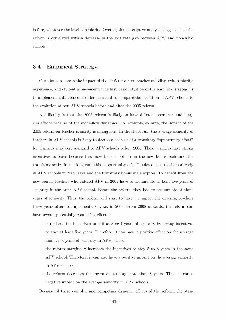
before, whatever the level of seniority. Overall, this descriptive analysis suggests that the

reform is correlated with a decrease in the exit rate gap between APV and non-APV

schools.

3.4 Empirical Strategy

Our aim is to assess the impact of the 2005 reform on teacher mobility, exit, seniority,

experience, and student achievement. The first basic intuition of the empirical strategy is

to implement a difference-in-differences and to compare the evolution of APV schools to

the evolution of non APV schools before and after the 2005 reform.

A difficulty is that the 2005 reform is likely to have different short-run and long-

run effects because of the stock-flow dynamics. For example, ex ante, the impact of the

2005 reform on teacher seniority is ambiguous. In the short run, the average seniority of

teachers in APV schools is likely to decrease because of a transitory “opportunity effect”

for teachers who were assigned to APV schools before 2005. These teachers have strong

incentives to leave because they now benefit both from the new bonus scale and the

transitory scale. In the long run, this “opportunity effect” fades out as teachers already

in APV schools in 2005 leave and the transitory bonus scale expires. To benefit from the

new bonus, teachers who entered APV in 2005 have to accumulate at least five years of

seniority in the same APV school. Before the reform, they had to accumulate at three

years of seniority. Thus, the reform will start to have an impact the entering teachers

three years after its implementation, i.e. in 2008. From 2008 onwards, the reform can

have several potentially competing effects :

- it replaces the incentives to exit at 3 or 4 years of seniority by strong incentives

to stay at least five years. Therefore, it can have a positive effect on the average

number of years of seniority in APV schools

- the reform marginally increases the incentives to stay 5 to 8 years in the same

APV school. Therefore, it can also have a positive impact on the average seniority

in APV schools

- the reform decreases the incentives to stay more than 8 years. Thus, it can a

negative impact on the average seniority in APV schools.

Because of these complex and competing dynamic effects of the reform, the stan-

142

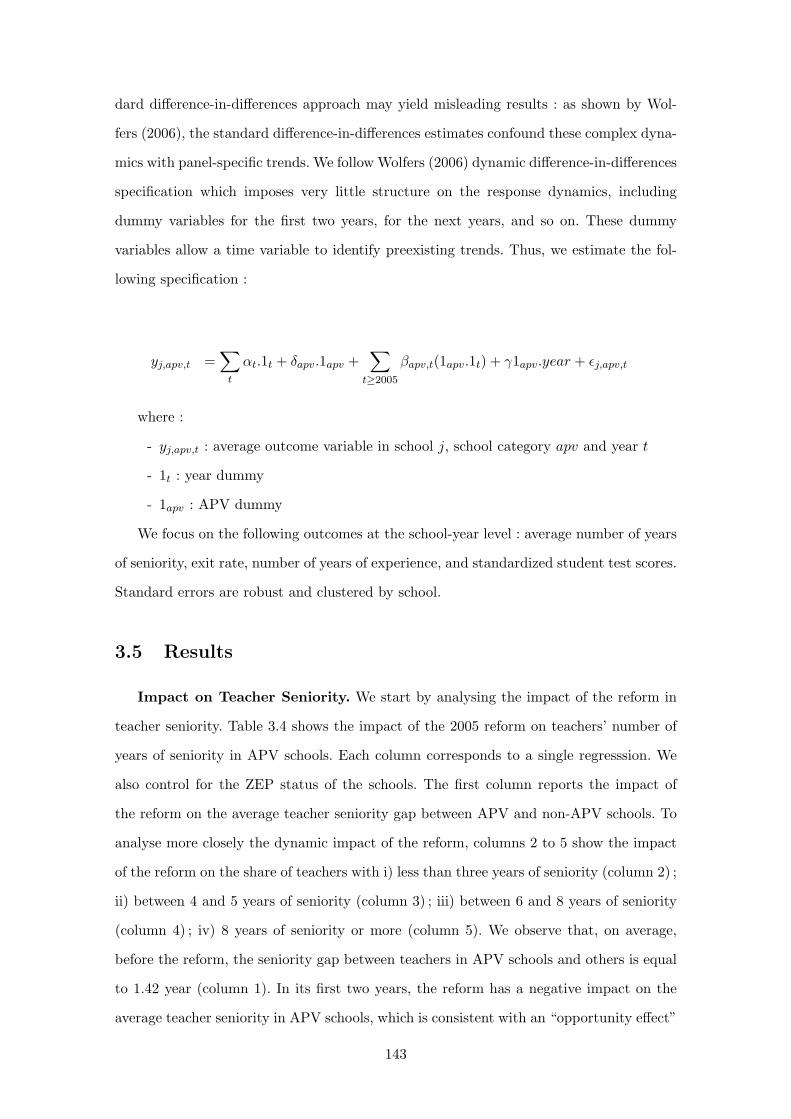
dard difference-in-differences approach may yield misleading results : as shown by Wol-

fers (2006), the standard difference-in-differences estimates confound these complex dyna-

mics with panel-specific trends. We follow Wolfers (2006) dynamic difference-in-differences

specification which imposes very little structure on the response dynamics, including

dummy variables for the first two years, for the next years, and so on. These dummy

variables allow a time variable to identify preexisting trends. Thus, we estimate the fol-

lowing specification :

yj,apv,t =∑

t

αt.1t + δapv.1apv +∑

t≥2005

βapv,t(1apv.1t) + γ1apv.year + ǫj,apv,t

where :

- yj,apv,t : average outcome variable in school j, school category apv and year t

- 1t : year dummy

- 1apv : APV dummy

We focus on the following outcomes at the school-year level : average number of years

of seniority, exit rate, number of years of experience, and standardized student test scores.

Standard errors are robust and clustered by school.

3.5 Results

Impact on Teacher Seniority. We start by analysing the impact of the reform in

teacher seniority. Table 3.4 shows the impact of the 2005 reform on teachers’ number of

years of seniority in APV schools. Each column corresponds to a single regresssion. We

also control for the ZEP status of the schools. The first column reports the impact of

the reform on the average teacher seniority gap between APV and non-APV schools. To

analyse more closely the dynamic impact of the reform, columns 2 to 5 show the impact

of the reform on the share of teachers with i) less than three years of seniority (column 2) ;

ii) between 4 and 5 years of seniority (column 3) ; iii) between 6 and 8 years of seniority

(column 4) ; iv) 8 years of seniority or more (column 5). We observe that, on average,

before the reform, the seniority gap between teachers in APV schools and others is equal

to 1.42 year (column 1). In its first two years, the reform has a negative impact on the

average teacher seniority in APV schools, which is consistent with an “opportunity effect”

143

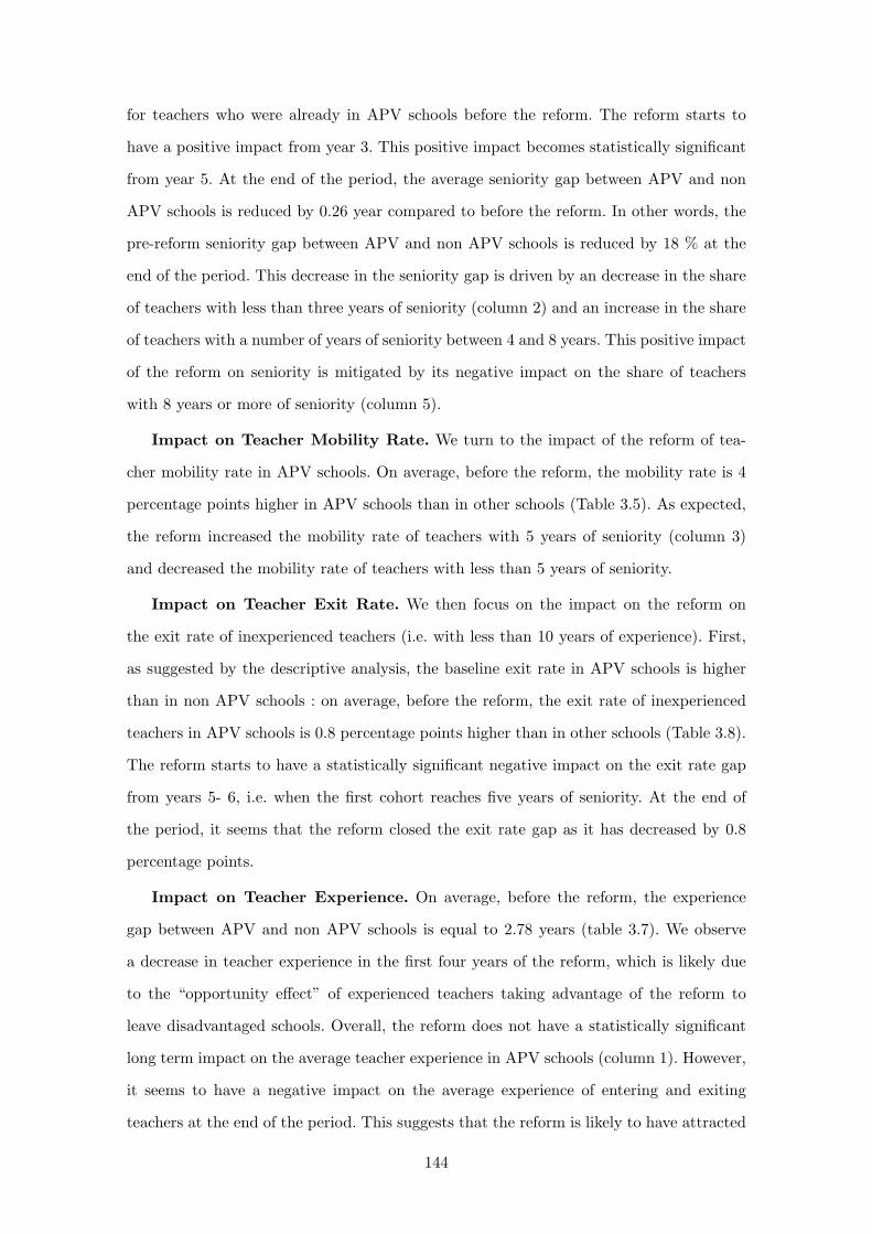
for teachers who were already in APV schools before the reform. The reform starts to

have a positive impact from year 3. This positive impact becomes statistically significant

from year 5. At the end of the period, the average seniority gap between APV and non

APV schools is reduced by 0.26 year compared to before the reform. In other words, the

pre-reform seniority gap between APV and non APV schools is reduced by 18 % at the

end of the period. This decrease in the seniority gap is driven by an decrease in the share

of teachers with less than three years of seniority (column 2) and an increase in the share

of teachers with a number of years of seniority between 4 and 8 years. This positive impact

of the reform on seniority is mitigated by its negative impact on the share of teachers

with 8 years or more of seniority (column 5).

Impact on Teacher Mobility Rate. We turn to the impact of the reform of tea-

cher mobility rate in APV schools. On average, before the reform, the mobility rate is 4

percentage points higher in APV schools than in other schools (Table 3.5). As expected,

the reform increased the mobility rate of teachers with 5 years of seniority (column 3)

and decreased the mobility rate of teachers with less than 5 years of seniority.

Impact on Teacher Exit Rate. We then focus on the impact on the reform on

the exit rate of inexperienced teachers (i.e. with less than 10 years of experience). First,

as suggested by the descriptive analysis, the baseline exit rate in APV schools is higher

than in non APV schools : on average, before the reform, the exit rate of inexperienced

teachers in APV schools is 0.8 percentage points higher than in other schools (Table 3.8).

The reform starts to have a statistically significant negative impact on the exit rate gap

from years 5- 6, i.e. when the first cohort reaches five years of seniority. At the end of

the period, it seems that the reform closed the exit rate gap as it has decreased by 0.8

percentage points.

Impact on Teacher Experience. On average, before the reform, the experience

gap between APV and non APV schools is equal to 2.78 years (table 3.7). We observe

a decrease in teacher experience in the first four years of the reform, which is likely due

to the “opportunity effect” of experienced teachers taking advantage of the reform to

leave disadvantaged schools. Overall, the reform does not have a statistically significant

long term impact on the average teacher experience in APV schools (column 1). However,

it seems to have a negative impact on the average experience of entering and exiting

teachers at the end of the period. This suggests that the reform is likely to have attracted

144

less experienced teachers, i.e. those who need the APV bonus the most, in APV schools.

Impact on Student Test scores. Finally, we analyse the impact of the reform on

the student test score gap. On average, before the reform, the student test scores gap

between APV and non APV schools is equal to 15 %. Overall, the reform does not have

any statistically significant impact on the student test scores gap between APV and non

APV schools.

This result has several possible interpretations. It may be because the positive impact

of the reform on teacher seniority is too small to have any statistically significant conse-

quence on student achievement. It may also be that the effect on seniority is mitigated by

the negative impact of the reform on the quality of teachers entering APV schools. This

mechanism would be consistent with a decrease in the experience of teachers entering

APV schools at the end of the period.

3.6 Conclusion

Most of the literature on teacher retention policies focuses on financial incentive

schemes and remains unconclusive. The present paper shifts the focus from financial

to non-pecuniary, career-oriented incentives. We analyse the impact of the disadvantaged

seniority bonus giving teachers in disadvantaged schools an extra mobility bonus once

they reach a certain level of seniority. We exploit as a natural experiment the 2005 reform

which both changed the set of disadvantaged schools benefitting from this extra seniority

bonus and the structure of this bonus.

We find that the reform has a positive impact on teacher seniority in APV schools. The

reform provokes a progressive decrease in the seniority gap between APV and non-APV

schools up to 20 % (0.44 years). We also find that the reform decreases the probability of

inexperienced teachers (i.e. with less than 10 years of teaching experience) in APV school

to leave the teaching profession. Finally, we find that the reform has no statistically

significant impact on the quality of teachers moving to APV schools, as measured by

their number of years of experience, nor on the student achievement gap between APV

and non-APV schools.

Further research. Further research will explore the underlying mechanisms under-

pining these results. First, we will try to understand why the average increase in teacher

145

seniority in APV schools does not have any statistical significant impact on the average

student achievement gap between APV and non-APV schools. A possible interpretation

is that the reform attracted lower quality teachers into APV schools. We will therefore

measure the evolution over time of the fixed effect of teachers entering APV schools.

Second, we will analyse the impact of the reform on teacher mobility applications.

Does the reform make APV schools more attractive ? We will therefore exploit data on

teacher applications to analyse the impact of the reform on the number of applications to

APV schools and on the characteristics of the applicants. This can also help us understand

the impact of the reform on inexperienced teachers exits from the teaching profession as

the reform may have given better school options to those vulnerable teachers.

3.7 References

Chetty, R., Friedman, J. N., Rockoff, J. E. (2014). Measuring the impacts of

teachers I : Evaluating bias in teacher value-added estimates. American Economic Review,

104(9), 2593-2632.

Clotfelter, C., Glennie, E., Ladd, H., Vigdor, J. (2008). Would higher salaries

keep teachers in high-poverty schools ? Evidence from a policy intervention in North

Carolina. Journal of Public Economics, 92(5-6), 1352-1370.

Darling-Hammond, L. (2015). Want to Close the Achievement Gap ? Close the

Teaching Gap. American Educator, 38(4), 14-18.

Goldhaber, D., Lavery, L., Theobald, R. (2015). Uneven playing field ? Asses-

sing the teacher quality gap between advantaged and disadvantaged students. Educational

researcher, 44(5), 293-307.

Hanushek, E. A., Kain, J. F., Rivkin, S. G. (2004). Why public schools lose

teachers. Journal of human resources, 39(2), 326-354.

OECD (2005). Attracting, Developing and Retaining Effective Teachers - Final Re-

port : Teachers Matter, 28/6/2005

Prost, C. (2013). Teacher mobility : Can financial incentives help disadvantaged

schools to retain their teachers ?. Annals of Economics and Statistics, 171-191.

Rockoff, J. E.(2004). ”The impact of individual teachers on student achievement :

Evidence from panel data.” American Economic Review 94, no. 2 : 247-252.

146

3.8 Tables and Figures

Figure 3.1 – Number of Seniority Points per Number of Years of Seniority

010

020

030

040

050

060

070

080

0S

enio

rity

Bon

us

1 2 3 4 5 6 7 8 9 10 11 12 13 14 15 16 17 18 19 20Number of Years of Seniority

Non ZEP - before ZEP - beforeNon APV - after APV - after

147

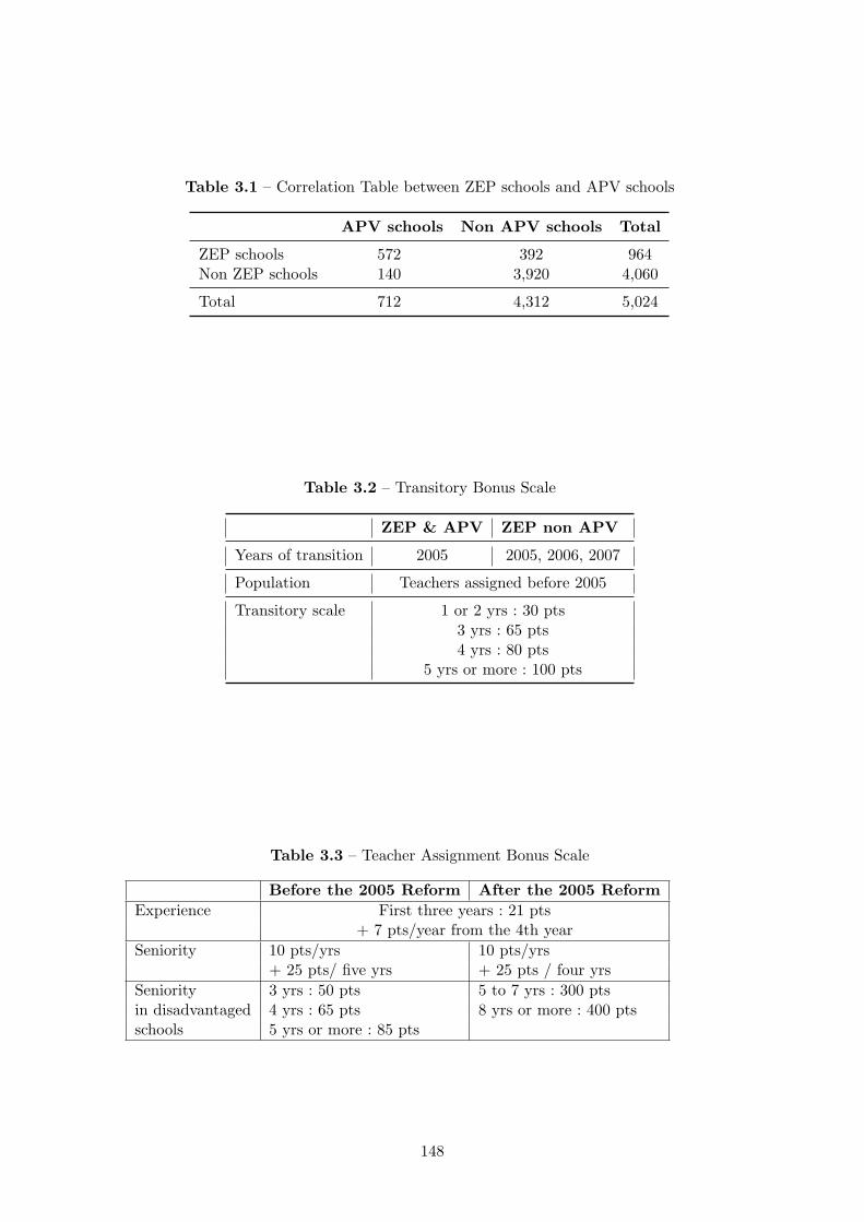
Table 3.1 – Correlation Table between ZEP schools and APV schools

APV schools Non APV schools Total

ZEP schools 572 392 964Non ZEP schools 140 3,920 4,060

Total 712 4,312 5,024

Table 3.2 – Transitory Bonus Scale

ZEP & APV ZEP non APV

Years of transition 2005 2005, 2006, 2007

Population Teachers assigned before 2005

Transitory scale 1 or 2 yrs : 30 pts3 yrs : 65 pts4 yrs : 80 pts

5 yrs or more : 100 pts

Table 3.3 – Teacher Assignment Bonus Scale

Before the 2005 Reform After the 2005 Reform

Experience First three years : 21 pts+ 7 pts/year from the 4th year

Seniority 10 pts/yrs 10 pts/yrs+ 25 pts/ five yrs + 25 pts / four yrs

Seniority 3 yrs : 50 pts 5 to 7 yrs : 300 ptsin disadvantaged 4 yrs : 65 pts 8 yrs or more : 400 ptsschools 5 yrs or more : 85 pts

148

Table 3.4 – Impact of the 2005 Reform on Teachers Number of Years of Seniorityin APV Schools (2002 - 2015)

Average Share with Seniority...Seniority ≤ 3 yrs 4 - 5 yrs 6 - 8 yrs 8 yrs or +

(1) (2) (3) (4) (5)

APV -1.42*** 0.07*** 0.01** 0.00 -0.08***(0.15) (0.00) (0.00) (0.00) (0.00)

ZEP -0.65*** 0.04*** 0.01** -0.01* -0.04***(0.13) (0.00) (0.00) (0.00) (0.00)

APV x Years 1 - 2 -0.21* 0.03*** 0.02** -0.04*** -0.00(0.12) (0.01) (0.00) (0.01) (0.00)

x Years 3 - 4 0.04 0.00 0.03*** -0.02** -0.02***(0.14) (0.01) (0.00) (0.00) (0.00)

x Years 5 - 6 0.24* -0.02* 0.05*** -0.00 -0.02**(0.14) (0.00) (0.00) (0.00) (0.00

x Years 7 - 8 0.31** -0.02*** 0.03*** 0.01* -0.02**(0.15) (0.00) (0.00) (0.00) (0.00)

x Years 9 - 10 0.26* -0.02* 0.02*** 0.01* -0.02**(0.16) (0.00) (0.00) (0.00) (0.01)

ZEP x Years 1 - 2 -0.06 -0.00 0.00 0.00 -0.00(0.11) (0.00) (0.00) (0.00) (0.00)

x Years 3 - 4 -0.10 -0.00 0.01* 0.00 -0.00(0.12) (0.00) (0.00) (0.00) (0.00)

x Years 5 - 6 0.00 -0.01** 0.00 0.01** -0.00(0.13) (0.00) (0.00) (0.00) (0.00)

x Years 7 - 8 0.19 -0.02** -0.00 0.02*** 0.01(0.14) (0.00) (0.00) (0.00) (0.01)

x Years 9 - 10 0.15 -0.01 -0.00 0.00 0.01(0.14) (0.01) (0.00) (0.00) (0.01)

Year Fixed Effect Yes Yes Yes Yes YesAPV pre-trend Yes Yes Yes Yes YesZEP pre-trend Yes Yes Yes Yes Yes

Nb of obs. 63,915 63.915 63,915 63,915 63,915

Note : Robust standard errors clustered by school. Each column corresponds to a singleregression. *** : 1 % level ; ** : 5 % level ; * : 10 % level.

149

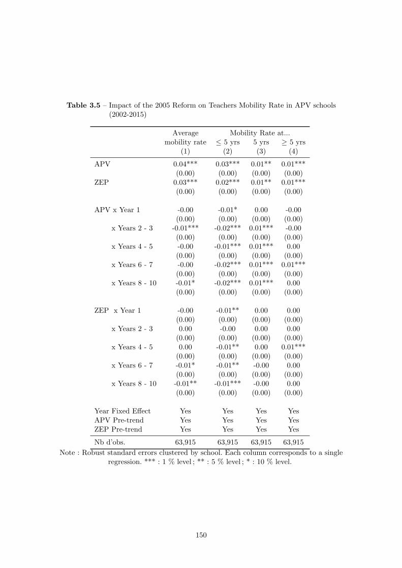
Table 3.5 – Impact of the 2005 Reform on Teachers Mobility Rate in APV schools(2002-2015)

Average Mobility Rate at...mobility rate ≤ 5 yrs 5 yrs ≥ 5 yrs

(1) (2) (3) (4)

APV 0.04*** 0.03*** 0.01** 0.01***(0.00) (0.00) (0.00) (0.00)

ZEP 0.03*** 0.02*** 0.01** 0.01***(0.00) (0.00) (0.00) (0.00)

APV x Year 1 -0.00 -0.01* 0.00 -0.00(0.00) (0.00) (0.00) (0.00)

x Years 2 - 3 -0.01*** -0.02*** 0.01*** -0.00(0.00) (0.00) (0.00) (0.00)

x Years 4 - 5 -0.00 -0.01*** 0.01*** 0.00(0.00) (0.00) (0.00) (0.00)

x Years 6 - 7 -0.00 -0.02*** 0.01*** 0.01***(0.00) (0.00) (0.00) (0.00)

x Years 8 - 10 -0.01* -0.02*** 0.01*** 0.00(0.00) (0.00) (0.00) (0.00)

ZEP x Year 1 -0.00 -0.01** 0.00 0.00(0.00) (0.00) (0.00) (0.00)

x Years 2 - 3 0.00 -0.00 0.00 0.00(0.00) (0.00) (0.00) (0.00)

x Years 4 - 5 0.00 -0.01** 0.00 0.01***(0.00) (0.00) (0.00) (0.00)

x Years 6 - 7 -0.01* -0.01** -0.00 0.00(0.00) (0.00) (0.00) (0.00)

x Years 8 - 10 -0.01** -0.01*** -0.00 0.00(0.00) (0.00) (0.00) (0.00)

Year Fixed Effect Yes Yes Yes YesAPV Pre-trend Yes Yes Yes YesZEP Pre-trend Yes Yes Yes Yes

Nb d’obs. 63,915 63,915 63,915 63,915

Note : Robust standard errors clustered by school. Each column corresponds to a singleregression. *** : 1 % level ; ** : 5 % level ; * : 10 % level.

150

Table 3.6 – Impact of the 2005 Reform on Teachers Average Number of Years ofExperience in APV schools (2002-2015)

Average Average experience of teachers...experience entering exiting

(1) (2) (3)

APV -2.78*** -2.26*** -1.45***(0.15) (0.20) (0.30)

ZEP -1.04*** -1.23*** -0.77***(0.13) (0.20) (0.29)

APV x Years 1 - 2 -0.48*** -0.17 0.02(0.12) (0.30) (0.38)

x Years 3 - 4 -0.24*** -0.03 0.10(0.12) (0.28) (0.37)

x Years 5 - 6 -0.15 -0.47* -0.46(0.13) (0.27) (0.38)

x Years 7 - 8 -0.15 -0.29 -0.85**(0.13) (0.29) (0.39)

x Years 9 - 10 -0.13 -0.99*** -1.19***(0.15) (0.32) (0.40)

ZEP x Years 1 - 2 -0.30*** 0.07 0.13(0.10) (0.29) (0.37)

x Years 3 - 4 -0.49*** -0.54** -0.52(0.11) (0.26) (0.36)

x Years 5 - 6 -0.44*** 0.17 0.16(0.13) (0.27) (0.37)

x Years 7 - 8 -0.31** -0.01 0.30(0.13) (0.28) (0.38)

x Years 9 - 10 -0.46*** 0.05 0.34(0.14) (0.30) (0.39)

Year Fixed Effect Yes Yes YesAPV Pre-trend Yes Yes YesZEP Pre-trend Yes Yes Yes

Nb d’obs. 63,915 63,915 63,915

Note : Robust standard errors clustered by school. Each column corresponds to a singleregression. *** : 1 % level ; ** : 5 % level ; * : 10 % level.

151

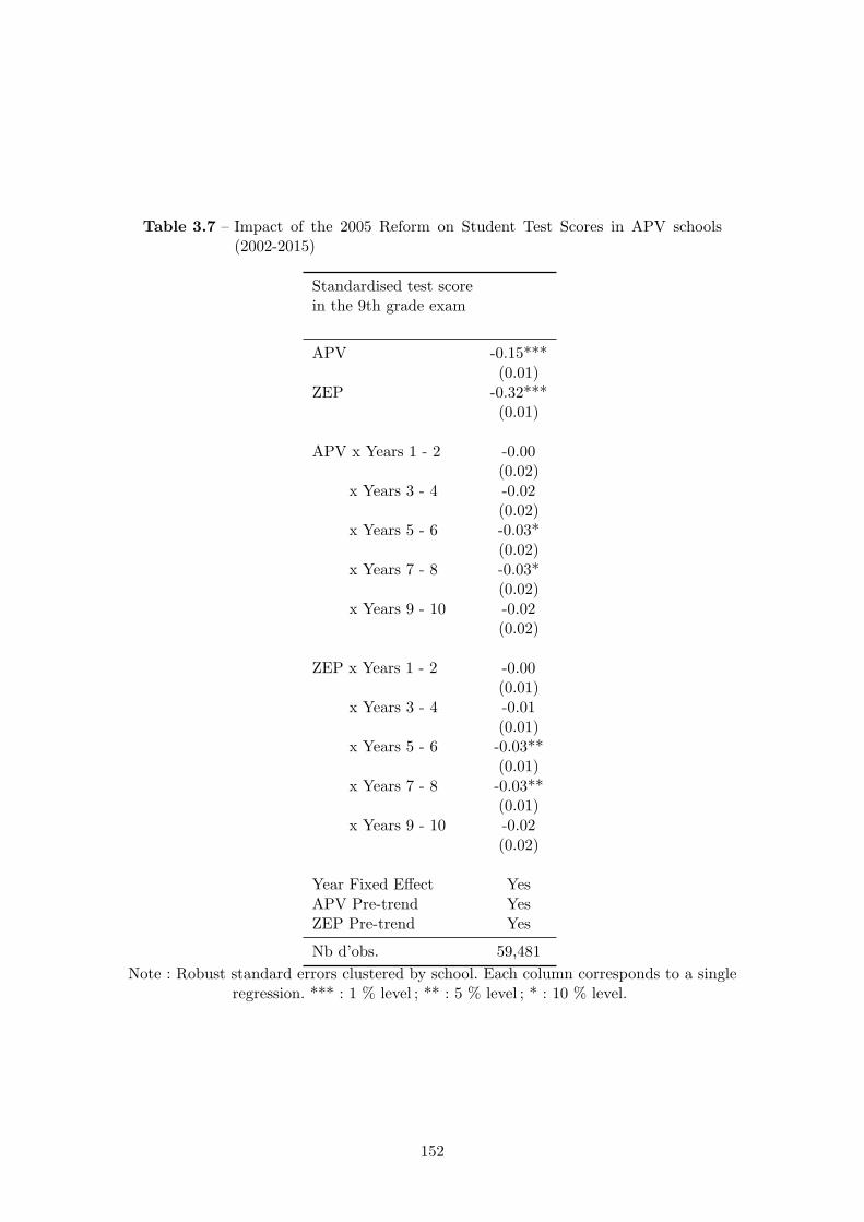
Table 3.7 – Impact of the 2005 Reform on Student Test Scores in APV schools(2002-2015)

Standardised test scorein the 9th grade exam

APV -0.15***(0.01)

ZEP -0.32***(0.01)

APV x Years 1 - 2 -0.00(0.02)

x Years 3 - 4 -0.02(0.02)

x Years 5 - 6 -0.03*(0.02)

x Years 7 - 8 -0.03*(0.02)

x Years 9 - 10 -0.02(0.02)

ZEP x Years 1 - 2 -0.00(0.01)

x Years 3 - 4 -0.01(0.01)

x Years 5 - 6 -0.03**(0.01)

x Years 7 - 8 -0.03**(0.01)

x Years 9 - 10 -0.02(0.02)

Year Fixed Effect YesAPV Pre-trend YesZEP Pre-trend Yes

Nb d’obs. 59,481

Note : Robust standard errors clustered by school. Each column corresponds to a singleregression. *** : 1 % level ; ** : 5 % level ; * : 10 % level.

152

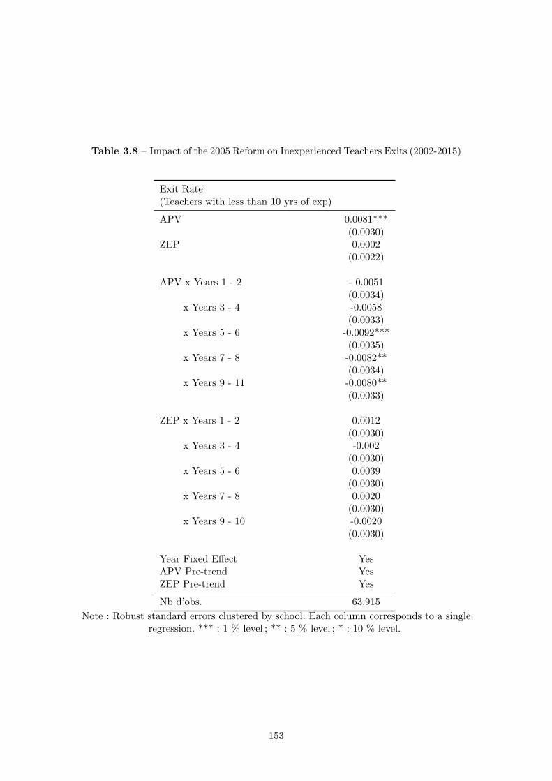
Table 3.8 – Impact of the 2005 Reform on Inexperienced Teachers Exits (2002-2015)

Exit Rate(Teachers with less than 10 yrs of exp)

APV 0.0081***(0.0030)

ZEP 0.0002(0.0022)

APV x Years 1 - 2 - 0.0051(0.0034)

x Years 3 - 4 -0.0058(0.0033)

x Years 5 - 6 -0.0092***(0.0035)

x Years 7 - 8 -0.0082**(0.0034)

x Years 9 - 11 -0.0080**(0.0033)

ZEP x Years 1 - 2 0.0012(0.0030)

x Years 3 - 4 -0.002(0.0030)

x Years 5 - 6 0.0039(0.0030)

x Years 7 - 8 0.0020(0.0030)

x Years 9 - 10 -0.0020(0.0030)

Year Fixed Effect YesAPV Pre-trend YesZEP Pre-trend Yes

Nb d’obs. 63,915

Note : Robust standard errors clustered by school. Each column corresponds to a singleregression. *** : 1 % level ; ** : 5 % level ; * : 10 % level.

153

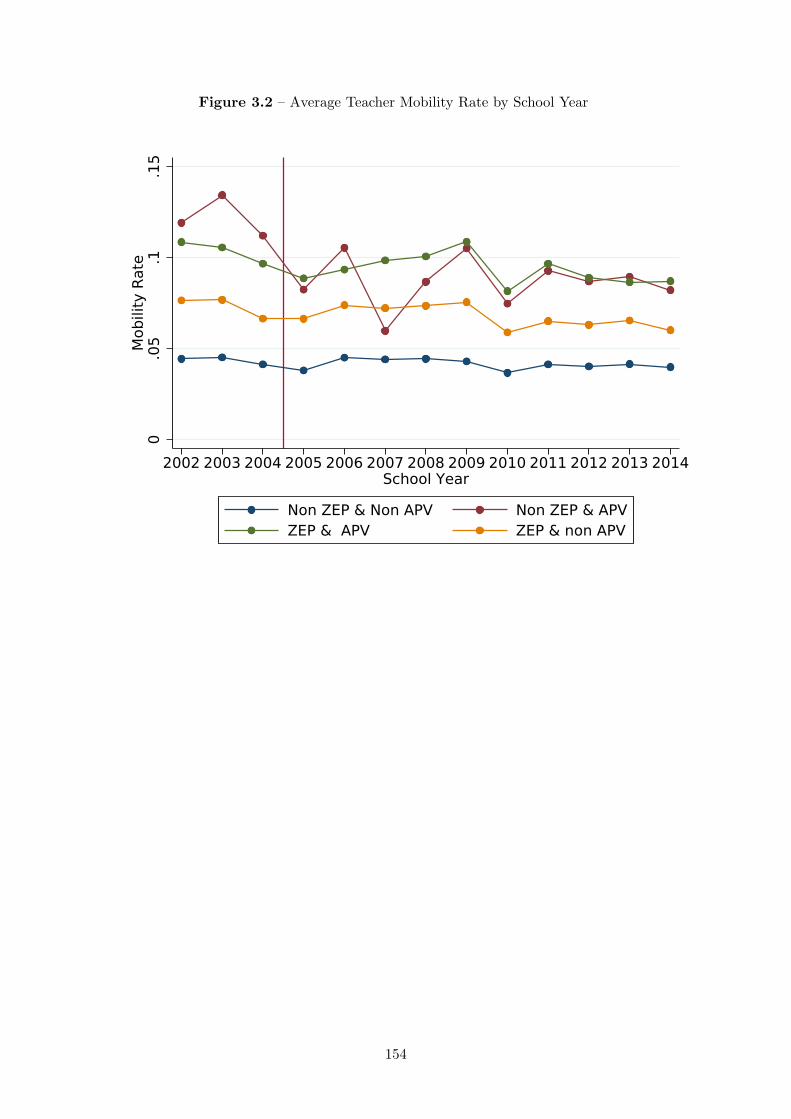
Figure 3.2 – Average Teacher Mobility Rate by School Year

0.0

5.1

.15

Mob

ility

Rate

2002 2003 2004 2005 2006 2007 2008 2009 2010 2011 2012 2013 2014School Year

Non ZEP & Non APV Non ZEP & APVZEP & APV ZEP & non APV

154

Figure 3.3 – Average Inexperienced Teacher Exit Rate by School Year

0.0

2.0

4.0

6.0

8Ex

it R

ate

2002 2003 2004 2005 2006 2007 2008 2009 2010 2011 2012 2013 2014Year

Non APV & non ZEP APV & non ZEPAPV & ZEP non APV & ZEP

Inexperienced teachers ; having less than ten years of experience.

155

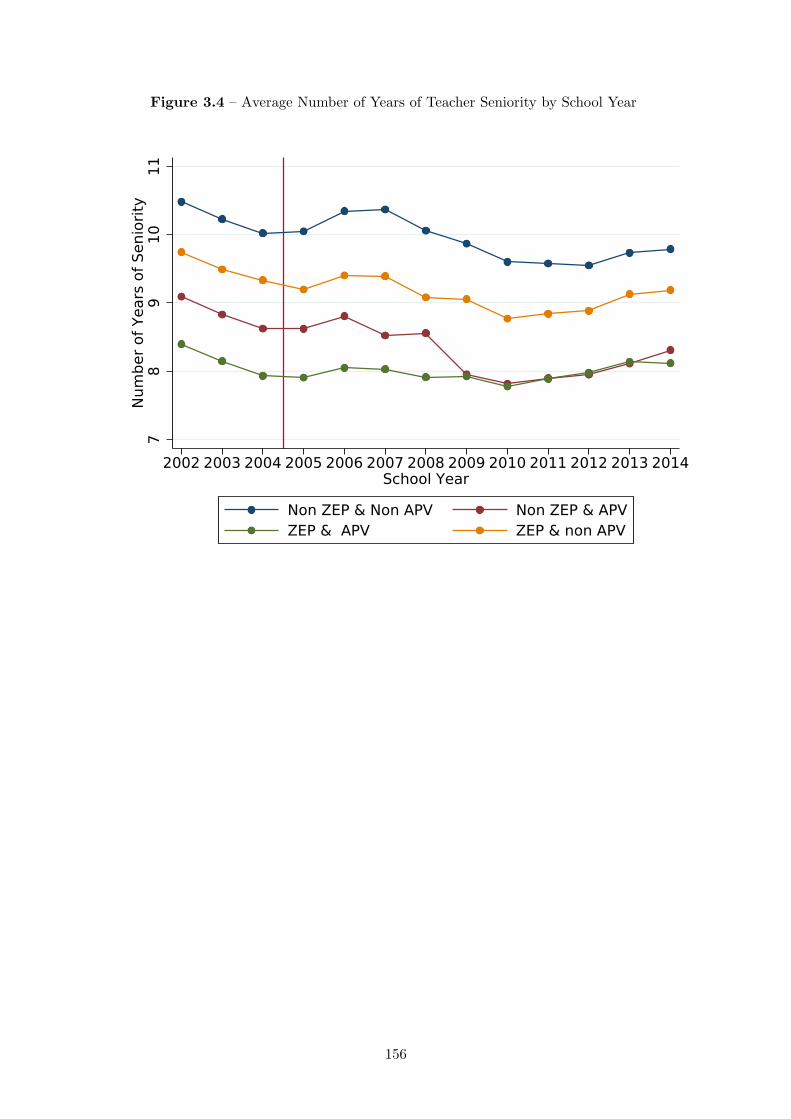
Figure 3.4 – Average Number of Years of Teacher Seniority by School Year

78

910

11Nu

mbe

r of Y

ears

of S

enio

rity

2002 2003 2004 2005 2006 2007 2008 2009 2010 2011 2012 2013 2014School Year

Non ZEP & Non APV Non ZEP & APVZEP & APV ZEP & non APV

156

Figure 3.5 – Average Number of Years of Teacher Experience by School Year

78

910

11Nu

mbe

r of Y

ears

of S

enio

rity

2002 2003 2004 2005 2006 2007 2008 2009 2010 2011 2012 2013 2014School Year

Non ZEP & Non APV Non ZEP & APVZEP & APV ZEP & non APV

157

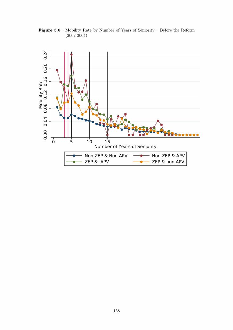
Figure 3.6 – Mobility Rate by Number of Years of Seniority – Before the Reform(2002-2004)

0.00

0.04

0.08

0.12

0.16

0.20

0.24

Mob

ility

Rate

0 5 10 15Number of Years of Seniority

Non ZEP & Non APV Non ZEP & APVZEP & APV ZEP & non APV

158

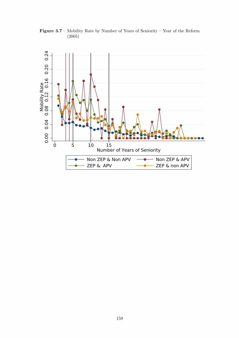
Figure 3.7 – Mobility Rate by Number of Years of Seniority – Year of the Reform(2005)

0.00

0.04

0.08

0.12

0.16

0.20

0.24

Mob

ility

Rate

0 5 10 15Number of Years of Seniority

Non ZEP & Non APV Non ZEP & APVZEP & APV ZEP & non APV

159

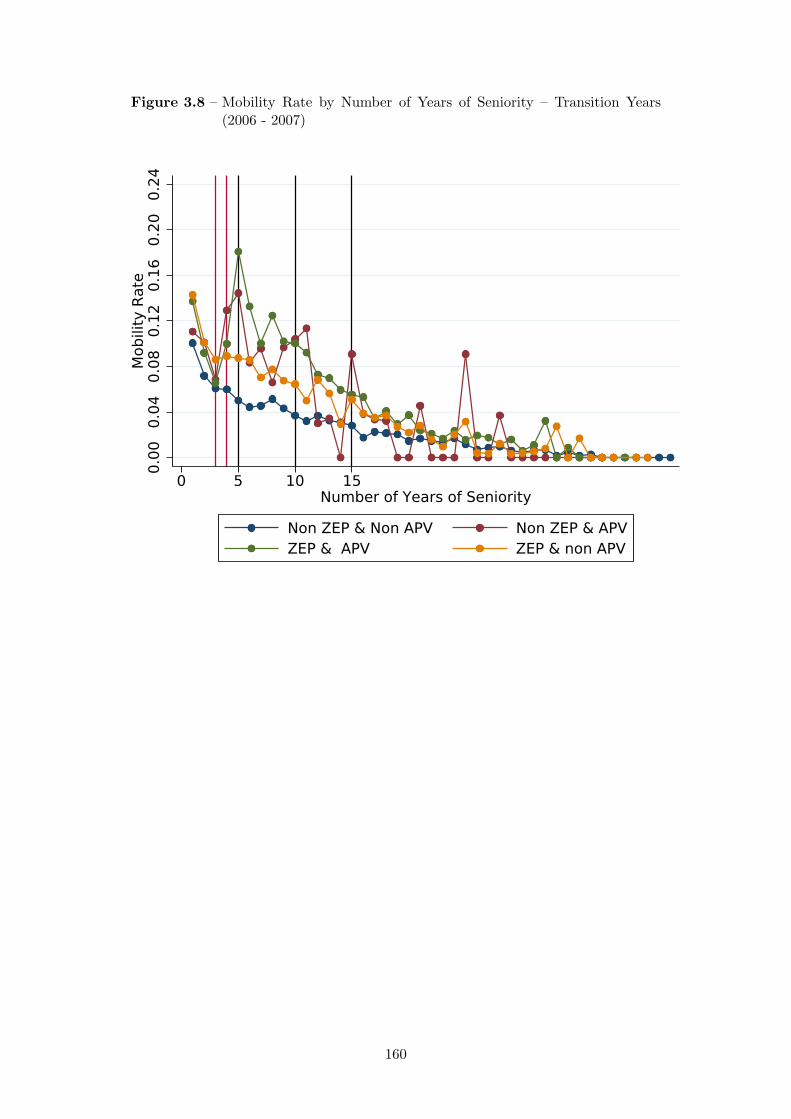
Figure 3.8 – Mobility Rate by Number of Years of Seniority – Transition Years(2006 - 2007)

0.00

0.04

0.08

0.12

0.16

0.20

0.24

Mob

ility

Rate

0 5 10 15Number of Years of Seniority

Non ZEP & Non APV Non ZEP & APVZEP & APV ZEP & non APV

160

Figure 3.9 – Mobility Rate by Number of Years of Seniority – After the Reform(2008 - 2014)

0.00

0.04

0.08

0.12

0.16

0.20

Mob

ility

Rate

0 5 10 15Number of Years of Seniority

Non ZEP & Non APV Non ZEP & APVZEP & APV ZEP & non APV

161

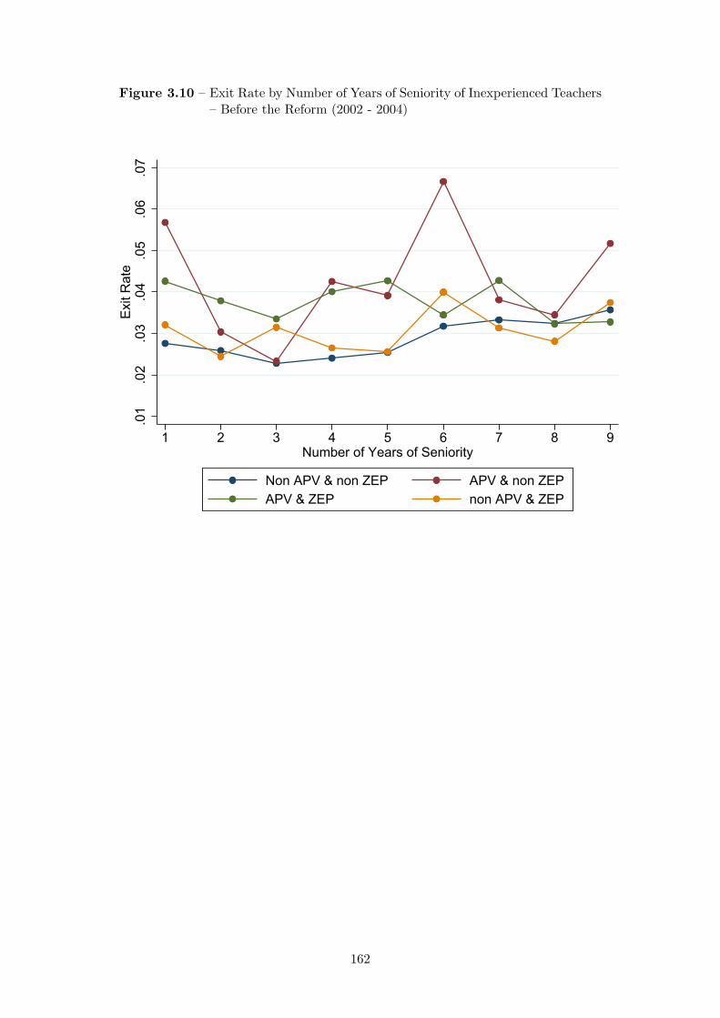
Figure 3.10 – Exit Rate by Number of Years of Seniority of Inexperienced Teachers– Before the Reform (2002 - 2004)

.01

.02

.03

.04

.05

.06

.07

Exit

Rat

e

1 2 3 4 5 6 7 8 9Number of Years of Seniority

Non APV & non ZEP APV & non ZEPAPV & ZEP non APV & ZEP

162

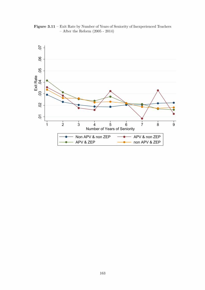
Figure 3.11 – Exit Rate by Number of Years of Seniority of Inexperienced Teachers– After the Reform (2005 - 2014)

.01

.02

.03

.04

.05

.06

.07

Exit

Rat

e

1 2 3 4 5 6 7 8 9Number of Years of Seniority

Non APV & non ZEP APV & non ZEPAPV & ZEP non APV & ZEP

163

Figure 3.12 – Average 9th Grade Student Test Scores Gap for Movers betweenPrevious School and New School

0.5

11.

5

Diff

eren

ce in

ave

rage

stu

dent

test

sco

res

(in s

tand

ard

devi

atio

n)

1 2 3 4 5 6 7 8 9 10Number of Years of Seniority

Non APV - Before non APV - AfterAPV - Before APV - After

164

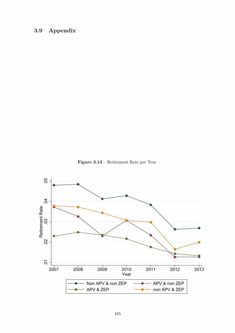
3.9 Appendix

Figure 3.13 – Retirement Rate per Year

.01

.02

.03

.04

.05

Ret

irem

ent R

ate

2007 2008 2009 2010 2011 2012 2013Year

Non APV & non ZEP APV & non ZEPAPV & ZEP non APV & ZEP

165

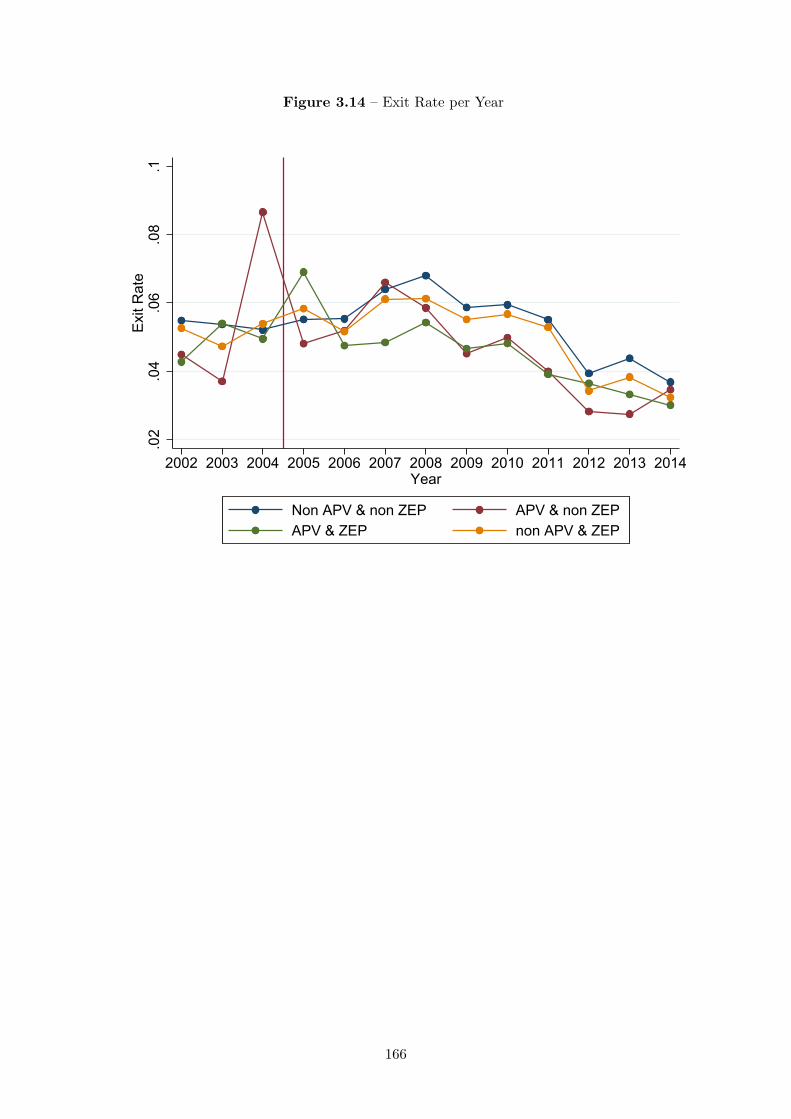
Figure 3.14 – Exit Rate per Year

.02

.04

.06

.08

.1Ex

it R

ate

2002 2003 2004 2005 2006 2007 2008 2009 2010 2011 2012 2013 2014Year

Non APV & non ZEP APV & non ZEPAPV & ZEP non APV & ZEP

166

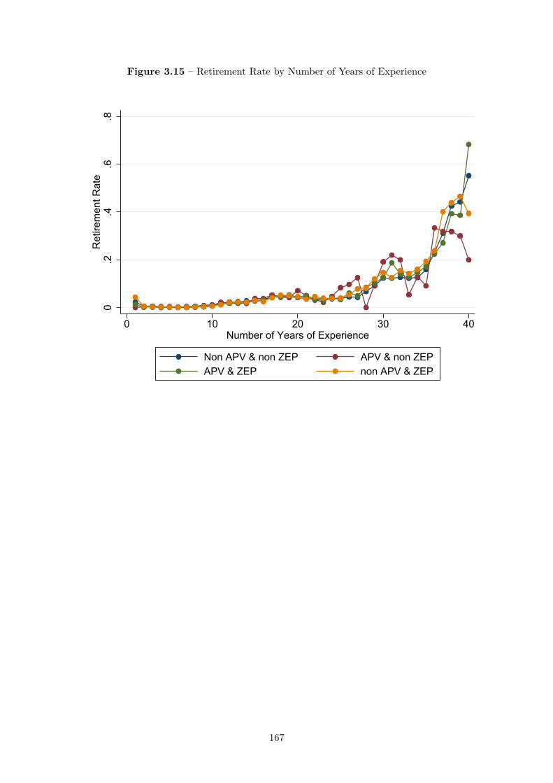
Figure 3.15 – Retirement Rate by Number of Years of Experience

0.2

.4.6

.8R

etire

men

t Rat

e

0 10 20 30 40Number of Years of Experience

Non APV & non ZEP APV & non ZEPAPV & ZEP non APV & ZEP

167