student academic achievement in rural

i

STUDENT ACADEMIC ACHIEVEMENT IN RURAL

VS. NON-RURAL HIGH SCHOOLS IN WISCONSIN

By Rebecca L. Droessler Mersch

A dissertation submitted in partial fulfillment

of the requirements for the degree of

DOCTOR OF EDUCATION

at

EDGWOOD COLLEGE

2012

ii

© Copyrighted by Rebecca L. Droessler Mersch 2012

iii

ABSTRACT

This study analyzed how Wisconsin rural public high schools’ academic achievement compared

to their city, suburb and town peers while controlling for ten factors. The Wisconsin Knowledge

and Concepts Examination (WKCE) measured academic achievement for tenth graders including

reading, language arts, mathematics, science and social studies. The ten independent variables

included geographic location, socioeconomic status, students of color, spending per pupil in the

school district, high school enrollment, parent education level, truancy, disciplinary actions:

suspensions and expulsions, students with disabilities and extra/co-curricular activity

participation. Data were provided by state and federal public databases. Findings indicated that

rural high schools in the state of Wisconsin performed as well as town and city high schools and

in some subject areas as well as suburban high schools. Further, the data suggest that there are

serious academic performance concerns for students and schools with certain demographics and

that those problems need to be addressed immediately and effectively. Findings from this study

suggest that the argument to consolidate rural high schools because of poor academic

performance is not a valid one. All high schools in Wisconsin including rural high schools

should be supported by policy makers and practitioners to ensure high academic achievement

opportunities for all.

iv

ACKNOWLEDGEMENTS

I would like to acknowledge several individuals that made this accomplishment possible.

First, thank you to my husband, Kurt, for his love, encouragement and support to pursue my

doctoral degree. Also, to my parents Gary and Julie and siblings Adam, Nathan and Sarah

Droessler for their unconditional love and support always.

I would also like to extend a sincere appreciation to Richard and Linda Barrows, Kitty

Flammang and the other members of Cohort IX for making this experience a wonderful journey.

Your intellect and life experiences have truly inspired me to be a better educator each and every

day.

v

DEDICATION

I would like to dedicate this study to all Wisconsin educators during this difficult political

climate. May you continue to be inspired to do the invaluable work that you do each and every

day.

vi

TABLE OF CONTENTS

ITEM PAGE

ABSTRACT……………………………………………………………………………….. iii

ACKNOWLEDGEMENTS………………………………………………………………. iv

DEDICATION……………………………………………………………………………. v

TABLE OF CONTENTS…………………………………………………………………. vi

LIST OF TABLES………………………………………………………………………... x

LIST OF FIGURES………………………………………………………………………. xii

CHAPTER 1 INTRODUCTION TO THE STUDY…………………………………... 1

Introduction………………………………………………………………………... 1

Historical Background…………………………………………………………….. 1

Measuring Rurality………………………………………………………………... 4

Contextual Orientation…………………………………………………………….. 5

Problem Statement………………………………………………………………… 7

Conceptual Model…………………………………………………………………. 7

Research Question…………………………………………………………………. 10

Significance of the Study………………………………………………………….. 10

Limitations of the Study…………………………………………………………… 12

Summary…………………………………………………………………………… 13

CHAPTER 2 REVIEW OF THE LITERATURE……………………………………..... 15

Introduction………………………………………………………………………... 15

Factors Affecting Academic Achievement………………………………………… 15

Socioeconomic Status……………………………………………………………... 16

Students of Color………………………………………………………………….. 18

Spending per Pupil………………………………………………………………… 22

School Size (High School Enrollment)……………………………………………. 25

Parent Education Level……………………………………………………………. 27

Truancy…………………………………………………………………………….. 30

Disciplinary Actions: Suspensions and Expulsions……………………………….. 33

Students with Disabilities…………………………………………………………. 36

Extra/Co-curricular Participation…………………………………………………. 38

Geographic Location………………………………………………………………. 40

Arkansas…………………………………………………………………… 40

Montana…………………………………………………………………… 42

North Dakota……………………………………………………………… 44

vii

Ohio……………………………………………………………………….. 46

Tennessee………………………………………………………………….. 47

Texas………………………………………………………………………. 50

West Virginia………………………………………………………………. 52

Benefits of Small Rural Schools on Communities………………………………… 53

Opposing Views: Pro-Consolidation………………………………………………. 56

Conclusion…………………………………………………………………………. 58

CHAPTER 3 METHODOLOGY………………………………………………………. 59

Methodology………………………………………………………………………. 59

Research Design…………………………………………………………… 59

Regression and Aggregation Bias: The Ecological Fallacy………………. 61

Data Sources………………………………………………………………………. 64

National Center for Educational Statistics (NCES)……………………….. 64

Wisconsin Information Network for Successful Schools (WINSS)………… 65

Wisconsin Department of Public Instruction (WDPI)……………………... 66

Wisconsin Department of Revenue (WDOR)………………………………. 67

Data Definitions…………………………………………………………………… 67

Academic Achievement……………………………………………………. 67

Geographic Location……………………………………………………… 70

Socioeconomic Status (SES)………………………………………………. 74

Students of Color………………………………………………………….. 76

Spending per Pupil………………………………………………………… 77

High School Enrollment…………………………………………………… 78

Parent Education Level……………………………………………………. 78

Truancy……………………………………………………………………. 80

Disciplinary Actions: Suspensions and Expulsions……………………….. 81

Students with Disabilities………………………………………………….. 82

Extra/Co-curricular Participation………………………………………… 83

Data Analysis……………………………………………………………………… 83

HPRB Approval…………………………………………………………………… 84

Summary…………………………………………………………………………… 84

CHAPTER 4 RESULTS……………………………………………………………….. 85

Results…………………………………………………………………………….. 85

Data Descriptions…………………………………………………………………. 86

Academic Achievement……………………………………………………. 86


Free and Reduced Lunch (SES)…………………………………………… 88

Students of Color…………………………………………………………... 89


High School Enrollment (School Size)…………………………………….. 91

viii

Average Income by School District (Parent Education Level)……………. 92

Truancy……………………………………………………………………. 92

Disciplinary Actions: Suspensions and Expulsions……………………….. 93

Students with Disabilities…………………………………………………... 94

Extra/Co-curricular Participation…………………………………………. 95

Data Correlations………………………………………………………………….. 96


Free and Reduced Lunch………………………………………………….. 98

Students of Color…………………………………………………………... 100


High School Enrollment…………………………………………………… 102

Average Income by School District………………………………………… 103

Truancy……………………………………………………………………. 104

Disciplinary Actions: Suspensions and Expulsions………………………... 105

Students with Disabilities…………………………………………………... 106

Extra/Co-curricular Participation………………………………………… 107

Regression Analysis………………………………………………………………... 108

Geographic Location………………………………………………………. 108

Reading……………………………………………………………………………. 109

All Variables Model………………………………………………………... 109

All Schools Model………………………………………………………….. 113

Analysis of Multicollinearity……………………………………………….. 116

Factor Analysis…………………………………………………………….. 118

Base Model Selection………………………………………………………. 121

Language Arts……………………………………………………………………... 124

Mathematics………………………………………………………………………... 125

Science……………………………………………………………………………... 127

Social Studies……………………………………………………………………… 129

Rural Location and Academic Achievement……………………………………… 130

CHAPTER 5 CONCLUSIONS, RECOMMENDATIONS & SUMMARY………….. 137

Conclusions, Recommendations & Summary……………………………………... 137

Introduction………………………………………………………………... 137

Research Conclusions……………………………………………………………… 139

Regarding Geographic Location and Achievement……………………….. 139

Regarding the Dependent Variables and the Other Independent Variables 140

Regarding the Independent Variables……………………………………... 141

Implications………………………………………………………………………... 145

Limitations of the Study…………………………………………………………… 148

Recommendations…………………………………………………………………. 150

Summary…………………………………………………………………………… 152

REFERENCES……………………………………………………………………………. 153

ix

APPENDIXES……………………………………………………………………………. 166

A.104 HIGH SCHOOLS…………………………………………………. 166

B. HIGH SCHOOLS INCLUDING OTHER GRADE LEVEL DATA… 167

C. OUTLIER SCATTER PLOTS………………………………………… 168

D. FACTOR_1 & FACTOR_2 COMPONENT MATRIX………………. 173

x

LIST OF TABLES

Table Title Page

Table 1 Conceptual Model………………………………………………………… 9

Table 2 Participation in Advanced Placement exams during the 2000-2001 school

year………………………………………………………………………...

19

Table 3 Percentage of students scoring a 3, 4 or 5 on the AP exam………………. 19

Table 4 1995-1996 Eighth graders who received a high school diploma in the

year 2000…………………………………………………………………

20

Table 5 Reading Proficiency based on school size………………………………... 45

Table 6 Math Proficiency based on school size…………………………………… 45

Table 7 State of Ohio survey results………………………………………………. 47

Table 8 Texas’ five athletic conference divisions, percentages of disadvantaged

students and proficiency percentages on the TAKS test…………………..

51

Table 9 Conceptual Model………………………………………………………… 60

Table 10 WKCE Proficiency Score Ranges – Grade 10……………………………. 69

Table 11 WKCE Point Differentials………………………………………………... 69

Table 12 National Center for Education Statistics (NCES) locale categories (2008) 71

Table 13 Geographical reclassification of 13 rural schools………………………… 73

Table 14 Income Eligibility Guidelines…………………………………………….. 75

Table 15 WKCE Descriptive Statistics……………………………………………... 87

Table 16 Geographical Location Descriptive Statistics…………………………….. 88

Table 17 Free and Reduced Lunch Descriptive Statistics………………………….. 89

Table 18 Students of Color Descriptive Statistics………………………………….. 90

Table 19 Spending per Pupil ($’000) Descriptive Statistics………………………... 91

Table 20 High School Enrollment Descriptive Statistics…………………………... 91

Table 21 Average Income by School District ($’000) Descriptive Statistics………. 92

Table 22 Truancy Descriptive Statistics……………………………………………. 93

Table 23 Disciplinary Actions: Suspensions and Expulsions Descriptive Statistics. 93

Table 24 Students with Disabilities Descriptive Statistics…………………………. 94

Table 25 Extra/Co-curricular Participation Index Descriptive

Statistics…………………………………………………………………...

95

Table 26 Geographic Location Data Correlations………………………………….. 97

Table 27 Free and Reduced Lunch Data Correlations……………………………… 98

Table 28 Free and Reduced Lunch Pearson (r) Correlations……………………….. 99

Table 29 Students of Color Data Correlations……………………………………… 100

Table 30 Students of Color Pearson (r) Correlations……………………………….. 100

Table 31 Spending per Pupil Data Correlations……………………………………. 102

Table 32 High School Enrollment Data Correlations………………………………. 102

Table 33 Average Income by School District Data Correlations…………………... 103

Table 34 Truancy Data Correlations………………………………………………... 104

Table 35 Truancy Pearson (r) Correlations………………………………………… 104

Table 36 Disciplinary Actions: Suspensions & Expulsions Data Correlations…….. 105

Table 37 Disciplinary Actions: Suspensions & Expulsions Pearson (r) Correlations 106

xi

Table 38 Students with Disabilities Data Correlations……………………………... 107

Table 39 Extra/Co-curricular Participation Data

Correlations……………………….. . . . . . . . . . . . . . . . . . . . . . . . . . . . ….

108

Table 40 All Variables Model – Regression 1……………………………………… 110

Table 41 All Schools Model – Reading…………………………………………….. 114

Table 42 Factor Analysis 1 – POVERTY & OUT_OF_SCHOOL………………… 119

Table 43 Factor Analysis 2 – FACTOR_1 & FACTOR_2…………………………. 121

Table 44 All Schools Model – Language Arts……………………………………… 124

Table 45 All Schools Model – Mathematics………………………………………... 126

Table 46 All Schools Model – Science……………………………………………... 128

Table 47 All Schools Model – Social Studies……………………………………… 129

Table 48 Base Model Regression Summary………………………………………... 131

xii

LIST OF FIGURES

Figure Title Page

Figure 1 Median Annual Earnings by Educational Attainment……………………. 79

1

CHAPTER 1

INTRODUCTION TO THE STUDY

Introduction

It is no secret, and Wisconsin is no exception, that public schools in the United States

have struggled to maintain a lucrative funding source to enhance and maintain educational

institutions. Due to declining enrollments in rural areas and increased costs to uphold current

school systems, school consolidation has become the answer for many legislators, policymakers,

and school districts in several states. In the state of Wisconsin, there are 417 public high schools.

Of those, 229 are located in rural areas (54.9%); 82 are located in towns (19.7%); 61 are located

in suburban areas (14.6%); and 45 are city schools (10.8%) (U.S. Department of Education,

2011). This research analyzed the impact rural high schools have on student achievement in the

communities in which they serve.

Historical Background

According to Bard, Gardener, and Wieland (2006), small schools date back to the 1800s.

One-room schoolhouses were very efficient in the times where there were not any paved roads

2

and automated transportation. In the early 1900s, there were over 200,000 one-room

schoolhouses in the United States (Purcell & Shackelford, 2005). Toch (2003) per Hylden stated

that most students only attended until the eighth grade and that only 35% of Americans attended

high school by the year 1910. Since high school was viewed as college preparatory, only about

4% attended college.

The invention of the automobile, new roads and the Industrial Revolution reformed the

way education had been for many years. A major campaign against child labor also took place

which made it more difficult for teenagers to find jobs, so students chose to stay in school.

Businesses also had a great influence on education and felt that the same policies used to run a

business could be transferred to the educational setting. The new methods were considered

economies of scale or more bang for your buck initiatives. Based on this theory, politicians and

school reformers decided that larger schools in the urban areas were the best model, and the rural

schools were considered inadequate (Lyson, 2002).

According to Hylden (2004), reformers such as Ellwood Cubberly, John Dewey and

James Conant influenced the future of education by supporting schools with enrollment in the

hundreds and thousands. The comprehensive high school was created as a large scale operation.

James Conant conducted several studies and wrote The American High School Today in 1959 in

which he recommended eliminating small high schools as a top priority. Cubberly expressed

school size in business or factory terms. As the Dean of Stanford’s School of Education, he

stated in 1916,

Our schools are, in a sense, factories in which the raw products (children) are to be

shaped and fashioned into products to meet the various demands of life. The

3

specifications for manufacturing come from the demands of the twentieth century

civilization, and it is the business of the school to build its pupils to the specifications laid

down. This demands good tools, specialized machinery, continuous measurement of

production to see if it is according to specification, the elimination of waste in

manufacture, and a large variety of output (Hylden, 2004, p. 5).

However, Bailey (2000) counters that argument based on efficiency. Rural school

dropout rates are much lower than urban areas and equal to more affluent suburb areas. He

argues that small schools cannot be considered inadequate when they continue to produce high

school graduates. In an era of accountability, with high school graduation being the benchmark,

large schools have yet to match the small school graduation rates. “When did educational

attainment, one of the historic, hallmark goals of public education, become inefficient?”(Bailey,

2000, p. 2).

The plummeting of the economy in rural areas also contributed to the consolidation

effort. During 1933-1970, more than 30 million people left their family farms for some other

occupation (Lyson, 2002). In addition, in 1954, the landmark case of Brown vs. the Board of

Education of Topeka, KS, the United States Supreme Court found segregation of schools

unconstitutional under the Equal Protections Clause under the 14th Amendment of the United

States Constitution. After this ruling, there were several additional school consolidations

throughout the United States (Bard et al., 2006).

In the 1930s, there were more than 130,000 school districts in the United States. By the

year 2000, there were less than 15,000 (Lyson, 2002). While the number of school districts was

decreasing by almost 90%, the United States population had doubled (Hylden, 2004). Currently,

4

the population of rural areas has continued to decline while the cost of educating students

continues to rise, with very little increase in government funding (Lyson, 2002).

A great debate has taken place for many years on the ideal enrollment number of a school

district that has the most positive effect on student achievement, attendance, and graduation

rates. Some experts argue that a district should have 4,000-5,000 students. Others recommend a

district enrollment of 750 students. Still others believe that an enrollment between 260-2,925

students is ideal. Despite the difference of opinion on ideal school district size, one statistic is

not in dispute: school spending is a U-curve with the smallest schools and the largest schools

costing more to operate than those in between (Bard et al., 2006).

Measuring Rurality

What is rural? According to Merriam-Webster (2011), rural is defined as “of or relating

to the country, country people or life….” Despite the simple dictionary definition, defining rural

is not an easy task. Typically, rural is defined by population size, population density, or distance

to a city of some size. According to the United States Department of Agriculture Economic

Research Service (ERS) (2007), there are nine definitions of rural based on three sources

including the United States Census Bureau, United States Office of Management and Budget

(OMB) and the ERS. Three definitions are based on census locations; three are based on census

urban area; one is based on the OMB Metropolitan Statistical Area; one is based on the ERS

rural-urban commuting area codes; and one is based on socioeconomic indicators provided by

the census bureau. In addition, the National Center for Education Statistics (NCES) has its own

set urban-centric locale categories released in 2006 including three city, three suburb, three town,

and three rural definitions.

5

As an official at the Wisconsin Department of Public Instruction (WDPI) has stated,

“Landing on a definition of rural is, as you have found, not as easy as one would think” (S.M.

Grady, personal communication, January 17, 2012). At WDPI, the Small Rural School

Achievement Program defined rural as districts with an NCES urban-centric code of 6, 7, or 8

and having fewer than 600 students enrolled in the school district. However, the federal Rural

and Low Income Grants require an NCES rural-centric code of 6, 7, or 8 with a poverty rate

greater than 20% and not eligible for the Small Rural School Achievement Program. Another, at

the state level is a sparsity aid program for school districts with less than 725 students, fewer

than 10 students per square mile and have at least 20% of the student population eligible for free

and reduced lunch. Lastly, WDPI also sometimes uses the NCES urban-centric locale codes.

The concept of rural may be intuitively clear, but it is not a fixed category. Another

complication arises when school districts fall into more than one category (S.M. Grady, personal

communication, January 17, 2012). For purposes of this study, geography will be defined by the

NCES urban-centric locale categories, specifically discussed in Chapter 3.

Contextual Orientation

In recent years, various states have created legislation to give incentives or mandates for

small schools to consolidate. For example, Silverman (2005) stated that the state of West

Virginia appointed a School Building Authority (SBA) to give stipends for school improvements

to buildings or facilities, remodeling or new building projects. The criterion to be considered for

these funds was that school districts needed to have a student enrollment that also met the state-

mandated enrollment number. If not, these schools were not considered for funding. This

prompted many districts to consolidate in order to get this funding. According to Silverman,

6

West Virginia spends more on school transportation than any other state in the United States;

however, their graduation rates and standardized test scores are just average.

Yet, Lyson (2002) found the statistical evidence to support the importance of a school in

a community: a) the gap between the rich and the poor is more common in communities without

schools than with schools; b) the number of households receiving public assistance is also higher

in communities without schools than with schools; c) the number of families receiving welfare

benefits is higher in communities without schools than with schools; and d) the child poverty

rates are also higher in communities without schools than those with schools.

Many states’ educational systems are in economic crisis due to the funding formulas and

the inadequacy to cover current costs. Many talk about finding tax relief but also funding reform

for schools – seemingly contradictory goals.

In Wisconsin, then newly elected, Governor Scott Walker, unveiled the 2011-2013

biennial budget this past March 2011. According to Stein, Marley & Berquist (2011), education

cuts were specified, including $834 million less in state aid to school districts compared to the

2009-2011 biennial budget. This loss equates to a 7.9% decrease in overall aid funding from the

previous biennium budget to K-12 public schools. Along with the decrease in state aid, the state

has also lowered the revenue cap on the number of dollars that can be collected through local

property taxes that provides a 5.5% decrease in the amount of local property tax and state aid that

will be received for each student. For example, the average revenue per student in Wisconsin is

approximately $10,100. The new budget decreased this funding by $555 for each student.

Those districts that spend more than the average would see a greater decrease versus districts that

7

spend less than the average. It can be argued that the current quality of education provided by

Wisconsin school districts may not continue to exist with fewer resources.

Since 229 of the high schools in the state of Wisconsin are considered rural, what is the

impact of these schools compared to their city, suburb and town peers? Are rural school districts

competing academically at a level that shows their positive impact not only to students, but also

to communities and governmental leaders?

Problem Statement

Within this study, rural high school student achievement was measured by performance

on the tenth grade Wisconsin Knowledge and Concepts Examination (WKCE) scores for the

2009-2010 academic school year. While controlling for ten variables (geographic location,

socioeconomic status, students of color, spending per pupil, high school enrollment, parent

education level, truancy, disciplinary actions: suspensions and expulsions, students with

disabilities and extra/co-curricular participation), rural student achievement was compared to the

performance of public city, suburb and town students in the state of Wisconsin. Data were

collected from multiple state and federal databases and analyzed by a multiple regression

analysis that compared the different variables using the Statistical Package for the Social

Sciences (SPSS) software.

Conceptual Model

The research interest in this study was the effect, if any, of rural location on student

performance. A very large body of research indicates that student achievement is related to

variables, such as family socioeconomic status, ethnic/racial group membership and other

8

factors, including some that are specific to the school setting. Any model to examine the effect

of rural location must control for these other factors that influence student achievement. The

statistical procedure of multiple regression analysis is designed to isolate the effect of one

variable while controlling for the effects of others. Thus, a multiple regression statistical model

was used in this study. The conceptual model drew on previous research analyzing the

determinants of student achievement, and the researcher’s interest in examining the effect of

rural location. The generalized conceptual model, shown in Table 1, depicts the dependent

variable of high school academic achievement, along with the ten independent variables that

were isolated during data analysis.

9

Table 1. Conceptual Model

Data Year: 2009-2010 (WINSS)

Dependent Variable:

HSA = High School Academic Achievement (percent of 10th

grade students proficient and advanced on the 10th

Grade WKCE tests in Reading, Language Arts, Mathematics, Science & Social Studies)

Independent Variables: G = Geographic Location (City, Suburb, Town, Rural)

S = Socioeconomic Status (SES) (percent of students receiving free & reduced lunch in the high school)

M = Students of Color (percent of students of color in the high school [Total Number of Students of Color/High

School Enrollment])

Sp = Spending per Pupil in the School District

P = High School Enrollment (based on September third Friday count by WDPI)

Pa = Parent Education Level (Average Income by School District [Total Income/Number of School District

Residents])

T = Truancy (percent of high school students truant)

R = Disciplinary Actions: Suspensions & Expulsions (total number of suspensions and expulsions as a percent of

high school enrollment [Number of Students Suspended + Number of Students Expelled/Fall Enrollment])

D = Students with Disabilities (percent of high school students diagnosed with disabilities)

X = Extra/Co-Curricular Activity Participation Rate Index (the sum of the percentage of students who participated in

the three sanctioned areas of school sanctioned activities)

Equation:

HAS(Reading) = f (G, S, M, Sp, P, Pa, T, R, D, X)

HAS(Reading) = a + b1G + b2S + b3M + b4SP + b5P + b6Pa + b7T + b8R + b9D + b10X

HAS(Language Arts) = f (G, S, M, Sp, P, Pa, T, R, D, X)

HAS(Language Arts) = a + b1G + b2S + b3M + b4SP + b5P + b6Pa + b7T + b8R + b9D + b10X

HAS(Mathematics) = f (G, S, M, Sp, P, Pa, T, R, D, X)

HAS(Mathematics) = a + b1G + b2S + b3M + b4SP + b5P + b6Pa + b7T + b8R + b9D + b10X

HAS(Science) = f (G, S, M, Sp, P, Pa, T, R, D, X)

HAS(Science) = a + b1G + b2S + b3M + b4SP + b5P + b6Pa + b7T + b8R + b9D + b10X

HAS(Social Studies) = f (G, S, M, Sp, P, Pa, T, R, D, X) HAS(Social Studies) = a + b1G + b2S + b3M + b4SP + b5P + b6Pa + b7T + b8R + b9D + b10X

The precise form of the equation and specification of the variables will be discussed in Chapter

3, so the variables in the above equation should be taken as generalized measures rather than

specific variables. For example, the general concept represented by the geographical location

10

variable may be specified in the regression equation as a series of binary (dummy) variables

representing three of the four categories. The research question was answered by examining the

statistical significance of the regression coefficient on the variable representing rural location.

The nature of the regression model, the precise form of the equation and the measurement of the

variables is the subject of Chapter 3. The equation is given in functional form, and then in the

form that was estimated using multiple regression analysis. Each of the equations depicts how

high school achievement, represented through the WKCE test for 10th

graders during the 2009-

2010 academic school year, was affected by the independent variables. The rationale for the

variables is developed in Chapter 2, and the precise definition and measurement of each of the

variables are presented in Chapter 3.

Research Question

The purpose of this study was to distinguish how rural Wisconsin high students performed on the

tenth grade WKCE in the areas of reading, language arts, mathematics, science and social studies

compared to Wisconsin city, suburb and town public high students.

Significance of the Study

Berry (2004) wrote, “Small schools, once derided as relics of the education system and

obstacles to national progress, now lie at the heart of one of America’s most popular reform

strategies…yet there has not been enough rigorous research examining the effects of school size

on student achievement” (p. 11). This study proposed to add to the research base.

Raywid (1999) cited several past studies that support the notion that small schools are

more effective than large schools. She cited a study conducted by Lee & Smith in 1995

11

examining 12,000 students from 800 high schools that found students had higher achievement in

smaller schools. She also cited supportive studies including a 1994 study in Philadelphia

conducted by McMullan, Sipe & Wolf where 20,000 students participated, a 1993 study

conducted by Huang & Howley of 13,000 Alaskan students and others that researched all

academic scores within a specific state. In 1994, Howley stated school size “exerts a unique

influence on students’ academic achievement, with a strong negative relationship linking the

two: the larger the school, the lower the student’s achievement levels” (Hylden, 2004, p. 13).

Similar studies have taken place in Arkansas, Kentucky, Montana, North Dakota, Ohio,

Texas and West Virginia comparing academic achievement and high school location (rural,

town, suburb or city). Per Silverman (2005), according to the Rural School and Community

Trust, students in rural states such as South Dakota, Nebraska, Montana and Wyoming were

continuing to achieve despite obstacles and high percentages of low SES within their schools.

The question remains as to how these states accomplished this task.

However, an analysis of academic achievement and geographic school type had never

been conducted in the state of Wisconsin. By isolating ten variables (including geographic

location, socioeconomic status, students of color, spending per pupil, high school enrollment,

parent education level, truancy, disciplinary actions: suspensions and expulsions, students with

disabilities and extra/co-curricular participation), this analysis brought depth in understanding

the relative academic competitiveness of public rural, town, suburban and city high schools in

the state of Wisconsin in the five core subject areas. This study was timely as funding for

Wisconsin public schools had been cut significantly for the next state biennial budget. State

12

lawmakers and educational leaders needed to know the value of rural schools as they debated

future school funding decisions.

Limitations of the Study

Several limitations to this study are important to note. First, in the research, student

achievement is said to be effected by many factors including socioeconomic status, ethnicity,

spending per pupil, school size, parent education level, student motivation and the relationship to

the teacher. In this current study, the first five of these factors were analyzed with respect to

student achievement. However, student motivation and relationship to teacher will not be

included in this study. Neither student motivation (Martin and Dowson, 2009; Meyer, Weir,

McClure, Walkey & McKenzie, 2009) nor relationship to teacher (Gehlbach, Brinkworth &

Harris, 2011) has statewide data available for Wisconsin. Therefore, analysis of these factors is

outside of the scope of this quantitative study.

Also, class size is sometimes said to impact student achievement (Blatchford, Bassett &

Brown, 2011). However, class size varies considerably within each high school regardless of the

school size. For example, a required class such as English may have 30 or more students while

an advanced level language class may have less than ten with both classes occurring within the

same high school. Since considerable variation exists within high schools of varying locations

and/or size, class size was not included as a factor in this study.

Another possible limitation to this study included the type of high schools in this study.

For the purpose of comparing city, suburban, town and rural schools, certain high schools were

excluded from this study. These excluded schools included parochial, alternative, charter, single

purpose and juvenile detention centers. Only traditional ninth through twelfth grade public

13

Wisconsin high schools were included in this study, so not all Wisconsin high school students

were accounted for in this study.

Further, another possible limitation may have resulted because some data included in this

study were school specific while others were district specific. The data differences will be

discussed further in Chapter 3. Also, this investigation was limited to the state of Wisconsin and,

therefore, the generalizability to other states is limited.

Additionally, as the measure being used to quantify academic achievement, the WKCE

scores, may or may not be the best reflection of a student’s aptitude based on several factors.

First, a student may experience test anxiety or a lack of motivation to do well as the 10th

grade

test is the seventh in a series of the WKCE exams students will participate in before they

graduate high school. Also regarding the WKCE scores, the definition of what is proficient and

advanced can be argued as arbitrary as the cut scores have changed over the years to ensure

adequate yearly progress (AYP) is met. For example, a student in the 40th

percentile in reading

is determined as proficient. Researchers may question if this is the best representation of

academic achievement.

While recognizing the limitations of this study, the researcher, nevertheless, believed that

the appropriate available measures could be chosen to best represent the constructs for this study.

Despite the limitations above, the researcher believed that the study had merit and could provide

reliable information.

Summary

In summary, the researcher was interested in knowing if Wisconsin rural public high

students were as academically competitive as their city, suburb and town peers. By gleaning this

14

information from this research study, the researcher hoped to provide salient evidence to the

significance of Wisconsin rural schools. Ultimately, the researcher intended to share the results

with state legislators and the Department of Public Instruction officials to assist them as they

develop public policy.

As Governor Walker continues to lead significant changes on how schools will be funded

in the future and with a recall election for the governor’s seat in the state of Wisconsin in June

2012, the political climate remains tense with several questions left unanswered. The researcher

has hope that this research study will provide evidence germane to this important public debate.

15

CHAPTER 2

REVIEW OF THE LITERATURE

Introduction

This study examined how rural students’ academic achievement compared to their

respective city, suburb and town peers. With 229 (54.9%) high schools in the state of Wisconsin

considered rural, the question was “How did rural students perform academically compared to

their peers?”

The literature review analyzed several factors that affect academic achievement, prior

studies on the impact of rural schools from several states, the research on the benefits of rural

schools and some opposing views about the benefits of rural schools with respect to school

consolidation.

Factors Affecting Academic Achievement

Several factors that impact student achievement are well documented within the

literature. They are geographic location, socioeconomic status, students of color, spending per

16

pupil, high school enrollment, parent education level, truancy, and disciplinary actions:

suspensions and expulsions, students with disabilities and extra-/co-participation and how they

may or may not influence academic achievement. Each factor will be reviewed separately with

geographic location, the central focus of this study reviewed last. That review will include

several studies from various states including the following: Arkansas, Kentucky, Montana, North

Dakota, Ohio, Tennessee, Texas, and West Virginia. Finally, the writings related to the

advantages and disadvantages of rural schools will be presented.

Socioeconomic Status

Research suggests that socioeconomic status (SES) may be a factor affecting academic

achievement. The U.S. Department of Education (2001) publishes statistics showing the

percentage of students attending schools in rural areas across several states. Examples of states

that have nearly one-half of rural student enrollments are the following: Vermont (56%), Maine

(54%) and South Dakota (46.8%). States that have the majority of their schools located in rural

areas include South Dakota (77.2%) and Nebraska (60.8%). Of those students who live in rural

areas, approximately 13.8% also live in poverty.

In the state of Mississippi, Coffey & Obringer (2000) outlined the problem of educating

the rural poor. Approximately 69% of all students live in low SES rural areas with 30% coming

from single-parent homes and 32% below the poverty line. The free and reduced lunch rate in

Mississippi is over 50% with 36% of those students coming from various ethnicities, including

African American, Asian American, Hispanic American and Native Americans. Academically,

students from Mississippi scored the lowest in the nation on the Iowa Test of Basic Skills (ITBS)

and the American College Test (ACT). The National Assessment of Educational Progress

17

(NAEP) tests demonstrated that only 18% of Mississippi fourth graders and 10% of eighth

graders were proficient in mathematics.

In the state of Tennessee, Hopkins (2005) analyzed student achievement with regard to

school location and the percentage of low SES students within the school. Schools were

defined by the percentage of students receiving free and reduced lunch. The schools were then

placed into three economic categories: 1) low to moderately disadvantaged (< 50% of students

receiving free and reduced lunch), 2) highly disadvantaged (50-74%) and 3) highest

disadvantaged (75% or higher). Hopkins (2005) collected data from the Tennessee State

Department of Education online public database including the 2002-2003 Tennessee

Comprehensive Assessment Program (TCAP) in mathematics for grades sixth, seventh and

eighth, the American College Test (ACT) for high school students and the SES of the school.

The school location information was collected from the National Center for Educational

Statistics (NCES) Public School Locator. Findings were consistent across all middle school

grades and high school ACT scores. Among all grade levels, schools categorized as other non-

rural ranked the highest in mathematics achievement followed by schools categorized as rural.

Schools designated as large central city schools scored the lowest and, notably, significantly

lower than the other non-rural and rural schools. Regarding the ACT, the variability among all

three locales was significant. The average mathematics ACT sub-score for other non-rural was

19.7326; for rural, 19.0562 and for large central city, 16.7079. After factoring in each level of

SES, the mathematics achievement measured by the ACT and location showed similar results.

Students from large central city schools showed a greater range of scores (5.5) than their other

non-rural (3.5) and rural schools (1.2) counterparts. For example, students from large central

18

city schools within the highest disadvantaged category had lower mathematics sub-scores than

students from large central city schools in the low to moderate disadvantaged category and their

other non-rural and rural counterparts. The range in scores among the different socioeconomic

categories were vast. Notably, the rural category had narrowest margin of scores regardless of

SES. Also, among the highest disadvantaged category, the rural schools performed the best

across all grade levels tested. The researcher then proposed that the rural schools have

characteristics that enhance achievement of students from the highest disadvantaged

backgrounds but admitted that defining these characteristics is still very unclear. Overall, this

study suggests that the higher the disadvantage, the lower the academic achievement. However,

if students are disadvantaged, it is better for them to be educated in a rural setting rather than in

other non-rural or large central city setting.

De Haan & MacDermid (1998) found that 75% of all poor students living in urban areas

in the United States have below average skills in reading and math, with 50% of those in the

lowest quintile. Thus, academic achievement in small schools is as good as or better than that of

larger schools, especially for students from low socioeconomic backgrounds. Therefore, SES is

an important factor with regard to academic achievement and will be included in this study.

Students of Color

In the state of Wisconsin, if a student has an ethnic background other than white, there

may be an influence on academic achievement. In 2003, Education Trust from Washington,

D.C., reviewed Wisconsin’s WKCE scores for fourth and eighth graders and compared them to

their respective National Assessment of Educational Progress (NAEP) equivalent scores to

determine if Wisconsin was narrowing the achievement gap between students of color and their

19

white peers. In 1998, Wisconsin was considered by the state to have the third largest

achievement gap for fourth grade students in reading.

The Education Trust (2003) also noted that students of color were also underrepresented

in both AP courses and Gifted and Talented programs as documented by Table 2 and Table 3.

Table 2. Participation in Advanced Placement (AP) exams during the 2000-2001 school year

Public K-12

Enrollment

Calculus AB

English Language &

Composition

Biology

African American 10% 1% 1% 3%

Asian 3% 4% 3% 3%

Latino 5% 1% 1% 1%

White 82% 94% 95% 93%

Total 100% 100% 100% 100%

Number 867,134 2,646 1,485 1,429

(Education Trust, 2003)

Table 2 displays the percentage of the student body population by ethnicity that

participated in the AP exams during the 2000-2001 school year. For example, of those taking the

AP Calculus AB exam, 94% of the students were White while the African American (1%), Asian

(4%) and the Latino (1%) student populations were much lower.

Table 3. Percentage of students scoring a 3, 4, or 5 on the AP exam

Calculus AB English Language &

Composition

Biology

African American * * 32%

Asian 64% 69% 54%

Latino 43% * *

White 73% 66% 57%

Total 71% 66% 56%

* Data not reported for those states that had fewer than 25 students take the test. (Education Trust, 2003)

20

Of those students taking an AP exam, only 32% of African American students scored a

passing mark on Biology while only 43% of the Latino population scored a 3, 4, or 5 on the

Calculus AB exam. The Asian population had comparable results to the white population. Of

the White student population, 73%, 66% and 57% scored a 3, 4 or 5 on the Calculus AB, English

Language and Composition and Biology, respectively (Education Trust, 2003). Overall, the

factor of ethnicity demonstrates a great disparity among those who graduated within the

traditional four years of high school as illustrated in Table 4.

Table 4. 1995-1996 eighth graders who received a high school diploma in the year 2000

8th

graders High School Diplomas Completion Rate

African American 5,424 2,573 47%

Asian 1,678 1,520 91%

Latino 2,096 1,446 69%

Native American 918 532 58%

White 55,672 52,474 94%

Total 65,788 58,545 89%

(Education Trust, 2003)

The white student population had a high school diploma completion rate of 94%; the

highest of all the other ethnic groups followed by the Asian (91%), Latino (69%), Native

American (58%) and African American (47%) student groups. Also, approximately 44% of

Wisconsin high school graduates will enroll in college compared to the national average of 54%.

African Americans are also known to have fewer college graduates than other ethnicities. In the

end, school districts that have high poverty rates and high enrollments of students of minorities

have found to also have less money to spend per student (Education Trust, 2003).

A The New York Times article entitled “Racial Gap in Testing Sees Shift by Region”

(Dillon, 2009), discussed the racial gap in NAEP testing and how it has shifted from the south to

21

the north and Midwest. Historically, the achievement gap between black and white students was

most pronounced in the southern states. However, there has been shift over the past 20 years. A

report from the Department of Education based on data from the NCES showed that southern

states such as Alabama and Mississippi were no longer seeing the achievement gaps that

Connecticut, Illinois, Nebraska and Wisconsin are witnessing. From the 1992 NAEP testing, an

average white student’s score on the fourth grade math test was 227/500 while an African

American fourth grader’s average score was 192, showing a 35-point gap. In 2007, the average

math score for a white fourth grader was 248/500 while the average African American fourth

grader rose to 222, narrowing the gap from 35 to 26 points. In 2007, Wisconsin had the largest

black-white gap in the nation on the fourth grade math test (not counting the District of

Columbia) by an average of 10 points. Wisconsin also had the largest achievement gap in

reading and math in both fourth and eighth grades. The Milwaukee Public Schools (MPS) has

missed NCLB requirements for the past five years (Dillon, 2009). “Black kids in Wisconsin do

worse than in all these Southern states,” and among the reasons for this gap is that Wisconsin

educators “haven’t been focusing on doing what’s necessary to close these gaps,” Kati Haycock,

President of Education Trust (Dillon, 2009, p. 2).

Most recent WKCE results provided by WINSS (2012) for the fall of 2010 showed the

following ethnic subgroups tested proficient and advanced in grade 4 reading: American Indian

(77.7%), Asian (80.6%), Black (60.3%), Hispanic (69.6%) and White (88.5%). In grade 8

mathematics, proficient and advanced results were the following: American Indian (67.8%),

Asian (79.3%), Black (44.7%), Hispanic (63.2%) and White (84.9%). Lastly, proficient and

advanced results for science in grade 10 demonstrated the following: American Indian (60.8%),

22

Asian (66.9%), Black (34.4%), Hispanic (50.3%) and White (82.1%). Overall, the white

students significantly did better on the test than their peers of color. This evidence supports the

theory of the achievement gap among students of color in the state of Wisconsin and, therefore,

warrants attention and will be included within this study.

Spending per Pupil

Spending per pupil may be a factor affecting academic achievement. In 1993, a study in

the state of Illinois discussed the relationship between spending per pupil and academic

achievement. Sharp (1993) collected data from 655 schools for grade 11 and 2,347 schools for

grade 3. At the time, state assessments in reading and mathematics were given to grades 3, 6, 8

and 11. The language arts assessment was given at grades 3, 6 and 8. This state assessment was

used to measure academic achievement. A Pearson r correlation was used to analyze if there was

a relationship between operating expenditures per pupil for the 1989-1990 academic school year

and the state test results from April 1991. On average, spending per pupil for the state of Illinois

at that time was $4,424. The school district with the lowest spent $2,253 per pupil. The highest

spending per pupil was $14,316. All data were collected from the Illinois State Department of

Education. Sharp’s 1993 study results showed a small but significant negative correlation

between spending per pupil and academic achievement for all grade levels and all subjects

except grade 11. It was found that there was no relationship between the variables at grade 11.

Overall, this finding showed that spending more money per pupil did not necessarily guarantee

higher academic achievement. The author suggested one reason for this may be that the majority

of school costs are used for employee salary and benefits, not specific programming. Previous

studies done in Arkansas (Klingele & Warrick, 1990), New York (Wendling & Cohen, 1981)

23

and Virginia (Connors, 1982) found increased spending per pupil did enhance students’

achievement. If money was spent on resources directly related to student instruction, there was

an increase in student achievement. However, if the additional funding was spread equally

across the budget and mostly on personnel, a relationship between the two variables was not

found. This issue was more about how the money was spent versus how much money was spent.

An additional factor to take into consideration was special education costs and how they may

skew the overall spending per pupil since they increase the overall average spending (Sharp,

1993).

In 1989, Howley did a follow-up study to the 1987 Walberg and Fowler’s study on

school district efficiency based on spending per pupil and three SES variables (i.e. assessed

property evaluation, personal income and free and reduced lunch percentages). Efficient school

districts were defined as those whose spending per pupil was less than the state average, and

inefficient school districts were those that spent more than the state average per pupil. Academic

performances were measured through the Kentucky Essential Skills Test (KEST) in the areas of

reading, writing, math, spelling, library and research skills and the Comprehensive Test of Basic

Skills, Form U (CTBS/U) in the areas of reading comprehension, writing, math, spelling and

library skills for all grade levels. Scores were then compared to the efficient and inefficient

districts. The three main questions in this study included the following: 1) How does SES effect

spending to predict efficient school districts? 2) How does student achievement in those districts

that are considered efficient compare to inefficient districts? 3) Are efficient districts considered

small, rural or some other type of organization?

24

Howley’s (1989) data came from three resources: the Kentucky Department of

Education, the Northwest Regional Educational Laboratory and the Appalachia Educational

Laboratory (AEL). The author, Howley, chose Kentucky because it not only had the largest

number of rural districts at 178, but also had testing data for all grade levels from the 1985-1986

school years. He also defined smallness by the AEL definition of a county district less than

3,000 students and an independent district less than 1,500 students. Of Kentucky’s districts, 40

independent districts and 61 county districts were classified as small. Ruralness was defined as

the number of students per square mile. Within all districts, Kentucky had zero independent

districts and 88 county districts that were classified as rural.

Howley’s (1989) analysis was done in two parts. The first part explored the significance

of seven different variables on spending per pupil. These variables included enrollment,

nonurban population (%), personal income per student, poverty rates, free lunch rates, assessed

property valuations and student density. Of the seven, three variables were found to have a

moderate to significant effect on spending per pupil: assessed property valuation, personal

income per student and the free lunch rate. The districts were than categorized as efficient and

inefficient based on spending per pupil and SES. Analysis showed that 83 districts were

considered inefficient due to spending up to $1,309 per pupil above the average, and 95 districts

were considered efficient due to spending up to $1,308 less per pupil against the average. The

second part of the analysis compared the efficient and inefficient districts against achievement on

the KEST and CTBS/U tests. In all comparisons, districts considered inefficient (spending more

per pupil than expected) showed greater academic achievement than efficient districts (spending

less per pupil than expected). The overall finding was that the increased spending per student

25

affected academic achievement positively. This contradicted Walberg and Fowler’s (1987) study

stating that spending per pupil did not have an effect on academic achievement (Howley, 1989).

Overall, spending per pupil has contradictory results on whether its influence on

academic achievement is a positive or negative one. However, due to the sensitivity of the future

of funding for Wisconsin schools, the researcher regards spending per pupil as an important

factor and is included in this study.

School Size (High School Enrollment)

Recent research suggests that school size may be a factor affecting student achievement.

Raywid (1999) asked, “How big is small?” (p. 3). She found that several studies had been

performed on the optimal enrollment number at the high school level. The Cross City Campaign

for Urban School Reform conducted by Fine & Somerville in 1998 set the limit at 500 students

while another study conducted by Williams in 1990 recommended 800 students for high schools.

In 1996, the National Association of Secondary School Principals (NASSP) recommended a high

school size of 600 students; whereas, Lee & Smith (1997) suggested a range between 600-900

students in 1997.

On a national level, the U. S. Department of Education (1998) conducted a

Principal/School Disciplinarian Survey on School Violence to a nationally representative

population of 1,234 public schools, of which all responded. The survey requested the number of

specific crimes that occurred during the 1996-1997 academic school year as well as principal’s

perceptions, disciplinary actions and follow-up measure taken, if any. When comparing small

schools (less than 300 students), medium-sized (300 to 999 students) to larger schools (more

than 1,000 students), the larger schools were found to have 875% more crime, 270% more

26

vandalism, 378% more theft, 394% more physical assaults, 3,200% more robbery and 1,000%

more weapons cases than small schools. In addition, of all schools reporting, only 38% of the

small schools reported incidents while 60% of the medium-sized and 89% of the large schools

reported criminal activity. As learning environment is a key to academic achievement, one can

conclude that smaller schools are considered safer per this study.

Howley (2000) found poverty and school size have a strong influence on academic

achievement, both positively and negatively. For example, if students of poverty attend a large

school with a large percentage of low-income students, their academic achievement was lower

than those students of poverty who attended a smaller school with a large percentage of low-

income students. The relationship between academic achievement, school size and

socioeconomic status (SES) of students and their families has been found to be indirect but

applicable (Walberg & Fowler, 1987). This article review combined two of the factors within

this study, school size and SES. N. Friedkin and J. Necochea (1988) established the calculus

equation to measure the effect of varying SES levels. R. Bickel and C. Howley (2000) found

strong evidence of a positive indirect relationship between students from low socioeconomic

backgrounds attending smaller schools and academic achievement in the state of Ohio.

However, in Texas, they found a direct relationship. They also found weak evidence in

Montana, and no evidence in the state of Georgia (however, after conducting a multi-level

analysis, an effect was found not evident at the single-level layer). Thus, the following standards

were found to be true: 1) low SES communities achieve more with smaller schools, and 2) the

studies in all five states demonstrated equity in student achievement in smaller schools and

districts.

27

Further studies are clearly needed, but it is time for superintendents and policymakers to

begin considering the issue of scale: the complex relationship of class, school, and district

size in creating an environment in which excellence and equity function together to

reinforce one another for the benefit of impoverished communities (Howley, 2000, p.

10).

Only one researcher, Kennedy (1990) was found to contradict the previous studies and

stated that school size had little to no effect on student achievement. Although, specific school

size recommendations are conflicting, school size is an important factor to consider when

assessing academic achievement and will be included in this study.

Parent Education Level

Parents’ education level may also have an effect on academic achievement. Considerable

research has consistently shown that parents’ education level has a positive correlation to

predicting their children’s achievement (Smith, Brooks-Gunn & Klebanov, 1997; Haveman and

Wolfe, 1995; Klebanov, Brooks-Gunn & Duncan, 1994).

Davis-Kean (2005) studied the indirect relationship between parent’s education and

income and their children’s academic achievement. A national cross-sectional population of

children was used for this study containing survey data from the 1997 Child Development

Supplement of the Panel Study of Income Dynamics (PSID-CDS). These data were collected

since 1968 and included approximately 8,000 families. Of those, there were 868 8-12 year olds

(436 females, 433 males). This sample included 49% non-Hispanic European American and

47% African American children. The author used structural equation modeling techniques for

her statistical analyses. She proposed two hypotheses: 1) “Parents’ education and family income

28

influence children’s achievement indirectly through their association with parents’ educational

expectations and parenting behaviors that stimulate reading and constructive play and provide

emotional support in the home” (Davis-Kean, 2005, p. 295) and 2) that her predictions would

apply across different racial groups. The Primary Caregiver Interview was given to the parents

with an 88% response rate while the children were given the Woodcock-Johnson – Revised Tests

of Achievement in the areas of Letter-Word, Passage Comprehension, Calculations and Applied

Problems. All participants received a small gift for participating in the study. The average

education within the households was 13.34 years, just above a high school diploma. The average

income of the families was $48,178. As a part of their interview, parents were given a scale of 1

to 8 to predict how much education they thought their child would complete (1=11th

grade or less

to 8=M.D., Law, Ph.D. or other doctoral degree). The mean for this sample was 5, meaning

parents expected their children to graduate from a two-year college. Overall, the correlations

showed “…that parent education and income are moderate to strong predictors of achievement

outcomes” (Davis-Kean, 2005, p. 297). Of the author’s hypotheses, the first was supported

through her findings; however, her second hypothesis was not supported, and she did find that

race differences were significant when looking at the relationship of parent education and

academic achievement.

“Achievement motivation is defined as a disposition to strive for success and/or the

capacity to experience pleasure contingent upon success” (Acharya & Joshi, 2009, p. 72). These

authors also believed that other socioeconomic variables, such as parents’ level of education,

parents’ occupations and parents’ income also influenced academic achievement. Parents of 200

intermediate school students having four levels of education including high school, intermediate,

29

graduation and post graduation were given the Deo-Mohan achievement motivation scale (1985).

This assessment explored various areas of academics along with general interest, dramatics and

sports. The study had two objectives: 1) to study the mother’s influence on the four areas being

assessed and 2) to study the father’s influence on the four areas being assessed. Two hundred

adolescents volunteered for the study and were divided into four groups of 50 based on parent

education (i.e. high school, intermediate, graduation and post-graduation). The survey contained

50 questions, and the volunteers self-reported their parent’s education levels. The data were then

analyzed using SPSS, version 11.01 using the mean, standard deviation and a one-way

ANOVA test. The results revealed that the mother’s education level significantly and positively

impacted a child’s academic motivation. However, the significance took place in academics

only, not in the other three categories of general interest, dramatics and sports. There was also a

positive effect from the father’s education level. Overall, adolescents whose father had more

education had a higher achievement motivation than those fathers with less education. Also, the

results indicated that the higher the parent education level, the higher the motivation for

achievement in academic areas. Other elective areas were not found to have been influenced by

parent’s education level (Acharya & Joshi, 2009).

Acharya and Joshi (2009) also noted that the more parent involvement with the child and

his/her school, the higher the level of importance on academic motivation for the child. The

authors stated that through their meta-analyses, they found a positive correlation between parent

education and academic achievement. Acharya and Joshi supported Corwyn and Bradley’s study

in 2002 stating that the mother’s education had the most direct influence on the child’s cognitive

30

and behavioral development. Therefore, parent education level has significant influence on

academic achievement and will be included in this study.

Truancy

Daily attendance or non-attendance in school may affect academic achievement. During

the 19th

century, compulsory attendance laws were made in the United States and Europe. The

intent was having more students attend school and not be a part of the workforce (Baskerville,

Duncan, & Hutchinson, 2010). McCluskey, Bynum and Patchin (2004) stated that students who

are truant become at-risk for drug and alcohol abuse, minimal participation in community affairs

and have fewer job opportunities.

Blasik (2005) found in the Broward County School District in Florida, the sixth largest in

the United States, the higher the number of unexcused absences, the lower the performance on

state standardized tests. As the assistant superintendent for the Broward County Schools, the

purpose of her research was to conduct a longitudinal study spanning five and one half years.

Not only was she looking for trends in absenteeism, she was also interested in the impact

absenteeism may have on academic achievement measured by the Florida Comprehensive

Assessment Test (FCAT). Her method included the count of enrolled days, excused absences

and unexcused absences for each student of each school in the district. The data were provided

by the Total Educational Resource Management System database. Results showed that an

inverse relationship was found between unexcused absences and FCAT scores. Specifically, the

more unexcused absences a student had, the lower the FCAT score. No relationship between

excused absences and FCAT scores was significant.

31

Puzzanchera, C., Stahl, A., Finnegan, T., Snydeer, H., Poole, R., & Tierney, N. (2003)

noted that truancy is one of the early warning signs that a youth may participate in delinquent

activity. They also referenced a 2002 San Bernardino, California, review that stated 78% of all

California inmates admitted their first infraction with the law was during a time they were truant

from school. The same report stated 57% of violent crimes also took place during the time a

juvenile should have been in school.

Other researchers including Baker, Sigmon & Nugent (2001) separated the causes for

poor attendance into four categories: 1) family factors, 2) school climate factors, 3) economic

factors and 4) student factors and a fifth added later, 5) demographic factors (Cash & Duttweiler,

2006). The family factors were identified as living in poverty, domestic violence, drugs and/or

alcohol abuse, lack of parental supervision, lack of awareness of attendance laws and the value

placed on education. School climate factors were defined as safety, school size, relationships

with staff, inconsistent truancy procedures and the lack of meeting students’ needs for minority

populations. Economic challenges included parental employment, parents having more than one

job, student employment, single parent homes, high mobility rates, transportation and childcare

expenses. Student factors encompassed alcohol and/or drug abuse, mental health or physical

health problems, lack of social skills and poor academic achievement. Lastly, demographic

factors involved SES levels, delinquent peers, gang involvement, interracial tensions, sense of

community and recreational facilities for adolescents. Students with the highest truancy rates

have been found to have the lowest academic achievement and are most likely to drop out of

school (Dynarski & Gleason, 1999).

32

According to the Public Policy Forum, Schmidt and Lemke (2006) reported the negative

effects of truancy in Wisconsin’s southeastern school districts. Of 318,000 students enrolled in

this area’s public schools, 3.6 million days were missed during the 2005-2006 school year. This

represented 6.5% of the school year ranging from a 2.8% absenteeism rate in Whitefish Bay to a

10.9% rate in Milwaukee Public Schools (MPS). Milwaukee County saw an absenteeism rate of

8.7%; the absenteeism was 6.8% in Kenosha County, and Racine County students missed 5.2%

of school days. These three counties make up the three largest school districts in southeastern

Wisconsin, ranking one, two and seven overall for absenteeism. In addition, over two thirds of

the days missed due to suspensions took place in southeastern Wisconsin.

As a whole, students in southeast Wisconsin are performing below the state average. This

applies to all grade levels in reading, math and science WKCE scores. For the third year in a

row, 37 MPS schools were identified for improvement in 2005. In 2006, 34 MPS schools failed

to meet the NCLB requirements that identified them as needing improvement even though six of

ten categories did improve from the previous testing year. When Milwaukee, Kenosha and

Racine counties are removed from the equation, the region’s WKCE scores are higher than

scores for the rest of the state. The academic disparity between the suburban and urban schools

becomes very evident. Science, in particular, was much lower in this region than compared to

the state at every grade level. Overall, five of the top ten school districts for WKCE results were

located in Waukesha County; however, Milwaukee, Kenosha and Racine with the highest

enrollments were located in the bottom five (Schmidt & Lemke, 2006).

The student attendance rate is much higher in smaller schools than in larger ones. The

issues of truancy, discipline problems, violence, theft, substance abuse and gang involvement are

33

less in small schools. Therefore, truancy is a substantiated factor and will be included in this

study.

Disciplinary Actions: Suspensions & Expulsions

Exclusionary discipline, including school suspensions and expulsions, is one of the most

common forms of discipline used in order to maintain a safe and conducive school climate for

learning. However, the irony remains that students who are removed from such learning

opportunities may also suffer academically over time. Thus, school disciplinary actions

including suspensions and expulsions may affect academic achievement.

National data concludes that 7% of the school population missed a day of school due to

being suspended or expelled, which has doubled since the 1970s. This leads to two competing

hypotheses. The first suggests that by removing disruptive students from the learning

environment, the protection and preservation of learning of all other students is ensured.

However, the simultaneous consequence is that frequent student removal from school has a

negative effect on the academic achievement of the removed student (Rausch & Skiba, 2006).

Rausch & Skiba (2006) performed a study on the rates of school discipline and student

achievement for grades one through twelve in a Midwestern state for the 2002-2003 school year.

The results were disaggregated by race and controlled for poverty. All disciplinary, achievement

and socioeconomic data were downloaded from the state Department of Education database.

The study contained the following variables:

Out-of-school suspensions (OSS) or expulsion (EXP) rates for the entire school

grades one through twelve.

34

Achievement rates represented by the percent of students not receiving special

education services who scored proficient or higher in both the English/language

arts and mathematics subtests on the state accountability test, organized by racial

subgroup.

School type defined as elementary (grades one through five) or secondary (grades

six through twelve).

Minority percentage calculated by the sum of each minority group divided by the

school’s total enrollment.

Poverty rate based on the percentage of students receiving free or reduced lunch.

Two regression models containing 635 schools including 69 elementary schools

(10.87%), and 566 secondary schools (89.13%) were used in this analysis. The results indicated

that after accounting for poverty levels, 1) secondary schools had a higher OSS incident rate

compared to elementary schools; 2) OSS incident rates for African American students was

greater than those for White, Hispanic and Multiracial students, and 3) the differences by race

and school type did interact with one another. For the elementary schools, the African American

incident rate was significantly higher than the other three racial groups. However, at the

secondary level, the African American incident rates were higher than the White and Multiracial

rates but not statistically different from the Hispanic rate. For expulsions, secondary schools had

a higher incident rate than elementary schools; however, there was no significant effect based on

race or an interaction effect (Rausch & Skiba, 2006).

Regarding academic achievement, Rausch & Skiba (2006) noted that after controlling for

poverty, school type and race had a significant interaction effect with each other. At the

35

elementary level, White passing rates were significantly higher than the three other racial groups.

At the secondary level, the average White passing rates were the highest among the other racial

groups while the African American average passing rates were significantly lower than all the

other racial groups. Also, each racial group had different mean passing rates that were

significantly different from one another ranking the following from best to worst: White,

Multiracial, Hispanic and African American.

Lastly, the relationship between school discipline and academic achievement found that

1) OSS incident rates significantly predicted school achievement passing rates accounting for

17.1% of the total variation; 2) the socio-demographic factors accounted for an additional 36.1%

of the total variation, and 3) OSS and expulsion incident rates predicted some variation in

achievement passing rates. Overall, the higher the rates of expulsion and OSS predicted lower

percentages of students passing the state accountability test, after factoring for socio-

demographic influences. The authors’ research also concluded that the results from this study do

not indicate that suspensions and expulsions have a positive effect on school achievement but

rather are consistent with previous research that indicates a negative relationship between

exclusionary discipline and academic achievement. In summary, although the use of OSS and

expulsions are related negatively to achievement, socio-demographic variables only accounted

for 36-38% of the variation and did not fully explain the relationship. Based on these findings

and after accounting for poverty, an inverse relationship existed where OSS rates were the next

strongest predictor of achievement and expulsion rates being the second strongest predictor of

achievement (Rausch & Skiba, 2006).

36

In 2004, Rausch & Skiba evaluated the state of Indiana’s suspensions and expulsions data

and academic achievement. They reviewed the relationship between a school’s out-of-school

suspension and expulsion rates and the passing rate on both the math and English/language arts

subtests on the Indiana State Test of Educational Progress (ISTEP). Findings included schools

with higher rates of suspension and expulsion also experienced lower average passing rates on

the ISTEP. Schools with lower rates of suspension and expulsion experienced higher average

passing rates on the ISTEP. The authors delved further to see if this could be related to other

factors such as demographic variables. Upon further research controlling for poverty rate,

percentage of African American students, total enrollment, school type (elementary or

secondary) and geographic location (urban, suburban, town and rural), researchers found that

out-of-school suspension is negatively related to academic achievement. Thus, schools with

higher out-of-school suspension rates found lower achievement results on the ISTEP (Rausch &

Skiba, 2004). Therefore, school disciplinary actions including suspensions and expulsions are

established as an important factor regarding academic achievement and will be included in this

study.

Students with Disabilities

Academic achievement may also be affected by students with disabilities. The United

States public school system educates more than six million students with disabilities,

approximately nine percent of the school-age population. Of those, one third is of traditional

high school age. Through federal legislative efforts, such as the Individuals with Disabilities

Education Act (IDEA), No Child Left Behind (NCLB) and Response to Intervention (RTI),

students with disabilities continue to be included in the general education setting. A wide belief

37

has been that students with disabilities cannot achieve at the same level as those students without

a disability. This may be true in some cases, but it is also important to note that some students do

achieve at and above the average nondisabled student. Overall, academic achievement varies

widely across special education populations (Swanson, 2008).

Swanson (2008) also noted that according to the United States Department of Education’s

National Assessment of Educational Progress (NAEP), often known as the Nation’s Report

Card, students are assessed and categorized into four achievement levels: 1) below basic, 2)

basic, 3) proficient and 4) advanced. NAEP allows for the comparison of students with

disabilities versus general education students. In 2005, only 5% of twelfth grade students with

disabilities scored at or above the proficient level compared to their non-disabled peers on the

reading test. Approximately three quarters scored below the basic level. However, one should

not make generalizations about special education populations as each disability can vary

dramatically.

Swanson (2008) also referenced another analysis performed by the 2006 National

Longitudinal Transition Study-2 that investigated the academic and functional performance of a

nationally representative group of students with disabilities. Since the series of tests were based

on national norms, the researchers were able to make comparisons to the general education

population. Results showed that 16-18 year old students with disabilities did not perform as well

as their non-disabled peers on the academic assessments. In reading comprehension, only 12%

of students with disabilities reached the level that the average non-disabled student achieved on

this test. However, the disability diagnosis seemed to have a strong correlation to student

performance. For example, one quarter of students diagnosed with a visual impairment

38

performed at or above the national norms. But on the other end of the spectrum, less than one

percent of students with mental retardation reached the national norms. These same results held

true for the other academic-skill domains as well. Since all of the schools in this study are public

schools and serve special education needs, students with disabilities will be included as a

variable in this study.

Extra/Co-curricular Participation

A question often asked is if participation in extra/co-curricular activities has a

relationship to academic achievement. Research suggests that extra/co-curricular participation

may affect academic achievement.

Dick (2010) studied a mid-sized high school in western Nebraska consisting of 850

students where 44% of the students participated in the free and reduced lunch program. Dick

(2010) offered ten research hypotheses. Relationships were found for five of the hypotheses, and

students who participated in extra-curricular activities were found to have the following: 1)

higher grade point averages (G.P.A.), 2) higher rate of school attendance, 3) students who

participated in sports only had a higher rate of discipline referrals, 4) students who were from

families of a higher socioeconomic status were more likely to participate in extra-curricular

activities and 5) white students were more likely to participate in extra-curricular activities than

students of color. The five hypotheses that were rejected because there was no relationship

between the variables were the following: 1) G.P.A. between students who participated in

athletics and students who participated in non-sport activities, 2) attendance between athletes and

non-athletes, 3) participation in extra-curricular activities and disciplinary referrals, 4) G.P.A.’s

of students who participated in sports only activities, non-sport activities or both and 5)

39

attendance of students who participated in sports only activities, non-sport activities or both.

One of the main conclusions from this study was that a positive relationship exists between

participation in extra-curricular activities and academic achievement.

In the state of Wisconsin, Wiederholt (2009) performed a study reviewing alumni

perceptions in the small rural community of Cuba City. The class of 1993 (74 students) was

asked to participate in a survey that assessed the following two questions: 1) Does participation

in high school athletics affect academic achievement? and/or 2) Does participation in high school

athletics affect leadership development? The survey included three questions regarding the

impact of high school athletics on academic achievement by assessing the number of athletic

seasons each participated in, if the participants were on the honor roll and if they were inducted

into the National Honor Society. A total of 65 surveys were mailed to members of the class of

1993 with 36 of them being completed for a return rate of 55%. Findings indicated that a

positive relationship existed between participation in high school athletics and academic

achievement. On a four-point scale, there was a strong positive response to the statement,

Participation in high school athletics helped me develop skills that contributed to earning better

grades with an average response of 3.03.

Lastly, a 2001 study of North Carolina high school athletes revealed significant

differences between athletes and non-athletes including the following: 1) the average G.P.A. for

athletes was 2.98 while non-athletes was 2.17; 2) the average number of days absent for athletes

was 6.3 compared to 11.9 for non-athletes for a 180-day school year; 3) discipline referrals were

33.3% for athletes while non-athletes was 41.8%; 4) the dropout rate was lower for athletes at

.6% versus 10.32% for non-athletes and 5) the graduation rate for athletes was 99.4% versus

40

93.5% for non-athletes. This study among others can be accessed at National Federation of State

High School Associations (NFHS), 2011.

Based on the previously stated studies, participation in extra/co-curricular activities is

established as a likely factor affecting student achievement and will be included in this study.

Geographic Location

Geographic location may be a factor affecting academic achievement. Studies related to

geographic location and student achievement have been performed in a number of states. In

some studies, geographic location and one or more factors affecting achievement were also

analyzed. In the following section, several of those studies will be reviewed.

Arkansas

Johnson, Howley, and Howley (2002) conducted a study examining academic

achievement, school size and poverty and the relationship among the variables in 2002. Data

were collected from grades 4, 5, 6, 7, 8 and 9 from all Arkansas schools through state test scores

provided by the Arkansas Department of Education. Poverty was measured by the percentage of

students who received free and reduced lunch. Previous research by the same authors in Alaska,

California, Georgia, Montana, Ohio, Texas and West Virginia found that students coming from

poverty had better academic success in smaller schools, thus, narrowing the achievement gap

between students of poverty and their peers. The following study specifically details students in

the state of Arkansas.

The researchers specifically studied two effects. The excellence effect of school size,

“Does the size of a school or a school district affect its students’ academic performance, and

does the nature and extent of that effect depend on the level of poverty in the community?”

41

(Johnson et al., 2002, p.6). The equity effect – “Is poverty’s power over student achievement

greater in smaller or in larger schools?” (Johnson et al., 2002, p.6). The Arkansas researchers

found similar results as past studies. First, students from poverty performed better academically

in smaller schools than in larger ones. They also found that students from wealthier communities

achieved academically despite school size; however, the poorer the community, the larger the

gap. Second, the achievement gap between students from wealthier communities compared to

poorer communities was far less in smaller schools than in larger ones. Third, students from

poor families achieved better in smaller schools located within smaller school districts versus

smaller schools within larger school districts. Lower academic achievement among poor

students was greatest amongst larger schools within larger school districts. Lastly, African

American students who comprised the majority of the school population had three times the

negative relationship amongst academic achievement, poverty and school size (Johnson et al.,

2002).

Overall, Johnson et al., (2002) concluded the following:

The excellence effect of small schools by increasing the size of schools from Arkansas’s

poorest 50% of students would lower student performance on the state mandated testing.

The excellence effect of consolidating small school districts with free and reduced lunch

rates of 48% or more would also lower student performance on the state mandated tests.

The equity effect of small schools weakens the strength of poverty over academic

achievement and also diminishes the achievement gap between wealthy students and poor

students.

42

The equity effect of small school districts decreases poverty’s strength influence between

50-85%.

Montana

The Matthew Project study was conducted by Howley (1999), and supported by the Rural

Challenge Policy Program, comparing academic achievement to school size, SES and the

product of school size and SES in Montana, Georgia, Ohio and Texas. The author chose these

states to provide a variety in the geography, school organization, ethnic and racial diversity, and

rural and urban diversity. The findings for the state of Montana are discussed below.

Howley (1999) found five key findings throughout this study: 1) as of 1999, Montana led

the country in the National Assessment of Educational Progress (NAEP) test scores; 2) teachers

in Montana are not paid very well compared to the average teaching salary; 3) Montana does not

spend more per pupil than the national average for public funding; 4) people from Montana

support their schools financially more than other states, and lastly 5) income distribution among

Montana residents is fairly equal. The question becomes, how can Montana continue to have

high academic achievement from smaller schools with only spending an average amount per

student?

According to Howley (1999), “Poverty figures is the chief and most prevalent threat to

normal academic accomplishment among individuals” (p. 7). Based on previous studies in West

Virginia (Howley, 1996), Alaska (Huang & Howley, 1993) and California (Friedkin &

Necochea, 1988), the author noted that the poorer the community, the smaller the school or

district needed in order for high academic achievement. His interaction hypothesis stated that an

optimal size for a school or school district depends on the percentage of students from lower SES

43

backgrounds. Howley (1999) found it important to mention that previous studies have not found

there to be a significant difference in achievement and the size of the school, but the achievement

and size of the school is based on the population of low SES students.

All Montana students in grades 4, 8 and 11 were tested using the Comprehensive Test of

Basic Skills (CTBS), Iowa Test of Basic Skills (ITBS), and the Stanford Achievement Test

(SAT) respectively and were used as the dependent variables for this study. The independent

variables included the size of the school and its SES levels based on free and reduced meals

participation. The data were completed for a total of 176 K-6 elementary schools, 172 7-8 grade

schools and 167 9-12 high schools. The results showed a regression relationship as well as

correlations between SES levels and the achievement by the size of the school. First, the

regression results found the proper size conditions in order for students to achieve academically.

Second, the academic achievement of students varied based on the size of the school and its low

SES population ratio. Similar results were found, “…equity in achievement means breaking—or

at least substantially mitigating—the prevailing bond between SES and achievement” (Howley,

1999, p. 31). More importantly, researchers found that achievement in the poorer schools and

districts is equal to, if not better, than its more affluent counterparts. Most significantly were the

210 districts with eighth grades scores being studied which found there to be an effect size of 1/3

to ½ standard deviation units in support of the smaller, low SES districts. Also, across all grade

levels, the relationship between SES and achievement showed a 40% variance among the larger

districts and no significant results for the smaller districts.

Limitations of this study did include the three different assessments (i.e. CTBA, ITBS

and SAT) at the three grade levels and that no analysis was made that the assessments were

44

comparable. In addition, SES was difficult to measure as not all low SES families participate in

the free and reduced lunch program. Also, how schools recruit or solicit families to participate in

this program was different for each school and district.

North Dakota

North Dakota’s school system consisted of 118,600 students in 1995. By 2004, it had

declined to 99,421 students. In 2000, North Dakota’s Department of Public Instruction (NDDPI)

proposed consolidation of 214 school districts into 62 mega-districts to the state legislature. The

legislature denied such a proposal, but Tom Decker, a NDDPI employee and main developer to

the 62-school consolidation plan, persisted with another plan. Based on new regulations, the

NDDPI now required all schools to provide specific programs and courses, inevitably forcing

some schools to close who could not meet the requirements. Decker concluded that such smaller

schools did not have the resources in order for students to achieve academically as well as their

peers in the larger schools. Hylden (2004) conducted research on North Dakota’s academic

testing for all high schools in order to analyze reading and math proficiencies compared to the

size of their respective schools. The researcher was most interested in how students from small

schools compared to their larger peers and if Decker’s logic to consolidate school districts was

supported by quantitative evidence (Hylden, 2004).

Findings of his research concluded that the largest high schools had the worst test scores.

Small schools were found to perform at or better than their larger peers. Even those with a

population of less than 50 students outperformed all schools in all areas of reading proficiency.

In North Dakota, schools in the small and poorer communities performed better on the academic

testing than the wealthier cities of Fargo and Bismarck. “In fact, the very poorest and very

45

smallest schools outperform all other schools in the state in terms of reading proficiency”

(Hylden, 2004, p. 39). Enrollment and proficient data provided by the NDDPI is illustrated in

Table 5 and Table 6.

Table 5. Reading Proficiency based on school size

Reading Proficiency

School Size <50 50-100 100-150 150-250 250-500 >500

Proficiency 61.74% 59.64% 56.71% 59.94% 60.07% 55.44%

(Hylden, 2004)

For example, Table 5 illustrates that reading proficiency for schools greater than 500

students (55.44%) were the lowest when compared to all other schools based on size. The school

size with the highest reading proficiency had an enrollment of less than 50 students (61.74%).

Table 6. Math Proficiency based on school size

Math Proficiency

School Size <50 50-100 100-150 150-250 250-500 >500

Proficiency 39.25% 38.3% 37.88% 41.04% 39.2% 37.25%

(Hylden, 2004)

Table 6 also illustrates that schools with the lowest math proficiency were schools that

had enrollments greater than 500 students (37.25%). The schools with the highest math

proficiency had enrollments of 150-250 students (41.04%).

Hylden’s (2004) study indicated that the lowest proficiency rating in reading and math

were in high school populations exceeding 500 students.

All of this data, of course, is quite problematic for the NDDPI’s assertion that North

Dakota students in small schools are being underserved academically. Quite the contrary,

the data should lead one to argue precisely the opposite: it is North Dakota’s large

46

schools that are poorly serving their students, and North Dakota small schools that are

providing a better education (Hylden, 2004, p. 38-39).

The data shows no quantitative evidence to suggest that consolidating or closing North Dakota’s

small schools will increase student achievement.

Ohio

McCracken and Barcinas (1991) performed a study in Ohio with four major objectives:

1) is location of a school (rural or urban) related to school factors (i.e. class size, enrollment,

staff size, extra/co-curricular offerings and expenditure per pupil), 2) is location of school related

to demographic factors (i.e. gender, ethnic background, SES, parent education level, parental

expectations, grade point average), 3) is location of school related to occupational factors (i.e.

job expectations, job aspirations, expected income, likelihood of finding a job, and when the

occupational choice was made), and 4) is location of school related to post-secondary aspirations

(i.e. plans for post-secondary education, type of education, start date). Only two of these four

objectives (#1 and #2) are related to this study and will be discussed here.

Ten rural schools and five urban schools agreed to participate through a cluster sampling

and were selected at random. A survey for both the school administrator and students was used

for this study. A total of 529 students out of 767 rural seniors from the class of 1989 provided

parental permission and completed the survey (69% response rate). A total of 718 out of 834

urban students provided parental permission and completed the survey (86% response rate). All

15 administrators participated in the survey. Data analysis was performed using basic statistics

including frequency distribution, percentages, means, and standard deviations. These

characteristics of rural and urban secondary schools in Ohio are listed in Table 7.

47

Table 7. State of Ohio survey results

Rural Urban

Average Class Size 74 333

High School Enrollment 309 1368

Teachers (avg.) 24 79

Teacher Aides 0 2

Certified Support Staff 3 13

Administrator 1 5

Extra/co-curricular Offerings 107 262

Extra/co-curricular Participation 3.5 3.5

Spending per Pupil $2,657 $3,527

Ethic Population: White 94% 72%

General Curriculum 23% 9%

Vocational Curriculum 19% 27%

Academic Curriculum 58% 64%

Average G.P.A. 2.64 2.54

(McCracken and Barcinas, 1991)

Overall, several differences are apparent between the rural and urban school related to

school factors and demographics. Most notably, an increase in spending per pupil did not equate

to higher academic achievement based on grade point averages.

Tennessee

Under NCLB, rural and urban schools are treated the same although they are vastly

different. With requirements to meet Adequate Yearly Progress (AYP) and hire highly qualified

teachers, Crow (2010) felt that NCLB did not allow for the differences between urban and rural

schools. He believed it was more important to specify both rural and urban school’s specific

strengths and deficits to help understand their respective needs. His dissertation compared the

achievement scores of low SES public urban and low SES rural schools in the state of Tennessee

48

to see if there were statistically significant differences in the variables of ethnicity, economically

disadvantaged status, students with disabilities, and limited English language proficiency. Crow

(2010, p.1) stated, “Research has shown a significant factor of achievement gap is location, or

geography.” He proposes that there are institutional challenges for both rural and urban schools,

such as location, funding, student population and economic health of the area that suburb

communities do not face. Crow (2010) stated that rural America is currently changing from one

of ethnically uniform, traditional farming communities to one of multiethnic communities of

agricultural and manufacturing workers. Since 25.4% of all schools are located in rural areas

and 37.2% in urban areas in the United States, rural schools are not to be discounted (Sutton &

Pearson, 2002).

Crow (2010) analyzed the Tennessee Comprehensive Assessment Program (TCAP)

scores in mathematics and language for grades three to eight in 207 low SES public schools. A

low SES school was defined as one who had at least 75% of its students qualifying for free and

reduced lunch and breakfast programs. This would include any family with a gross income of

$31,765. A random sampling of 10 low SES urban and 10 low SES rural schools was selected

for the study in which twelve participated. The TCAP results included the three performance

levels of below proficient, proficient and advanced. The TCAP scores used were a three-year

average (2003-2006) of students who were proficient and advanced. Statistical analyses using

the Statistical Package of the Social Sciences included t tests to determine if there was

significance in test scores of students from rural and urban areas when considering the variables

of ethnicity, low SES, students with disabilities and English language learners. The results

49

indicated that 1) low SES percentage of students proficient in mathematics was significantly

higher in rural students versus urban students, 2) the low SES percentage of students proficient in

reading and language arts was also significantly higher in rural students versus urban students,

and 3) low SES students with disabilities from urban schools scored significantly lower than low

SES students with disabilities from rural areas. Overall, despite the fact that urban and rural

areas may share some of the same challenges such as recruiting high quality teachers and

obtaining proper educational funding, urban schools have significant academic achievement

consequences based on this study (Crow, 2010).

Another study conducted in the state of Tennessee examined eighth and twelfth grade

students’ math achievement based on school location, county location, class looping status, SES,

grade and class size and access to upper-level math courses. Winters (2003) specified questions

related to high school students that included 1) What, if any, relationship existed between twelfth

grade students’ ACT math achievement and its school location, county location, SES, and

twelfth grade class size? 2) Could ACT math achievement be predicted by school location,

county location, SES and the twelfth grade class size? and 3) What relationship, if any, existed

between school averages on the ACT math test and school location, county location, SES,

twelfth grade class size, average math class size, faculty size and access to higher-level math

courses? Of all the high schools in Tennessee, 98% of public schools that contained twelfth

grade students reported ACT math test mean scores. The author also distributed surveys to all of

the Tennessee math chairpersons and students from three rural Appalachian Tennessee counties

in upper math courses (above Geometry and Algebra II) with a return rate of 60%. Results

50

indicated that there was a significant interaction between the county location and the results of

the ACT math test. Students from rural Appalachian schools, rural non-Appalachian schools and

non-rural Appalachian schools had higher means on the ACT math test than non-rural non-

Appalachian schools. In summary, students from the poorest, rural sections of Tennessee

outscored students from non-rural Tennessee on the ACT math subtest.

Texas

Stewart (2009) performed a study to determine if there was a relationship between

academic achievement, size of the high school and SES. At the time of the study, there was

nearly an even split, with 55.6% low SES and 44.4% non-disadvantaged students. This study

compared traditional Texas high schools based on the University Interscholastic League (UIL)

athletic conference organization. The five athletic conferences based on high school size within

the state of Texas were as follows: 5A (1,985 students or more), 4A (950-1,984), 3A (415-949),

2A (195-414) and 1A (less than 195). To compare the size of the schools and SES, the high

schools were divided into quartiles based on low SES percentages and the location of the high

school. Low SES students were identified through the free and reduced lunch and/or families on

public assistance within each high school. Academic achievement was measured by the eleventh

grade Texas Assessment of Knowledge and Skills (TAKS) administered during the 2005-2006

school year. These data were provided through the Texas Education Agency (TEA) online

program named the Academic Excellence Indicator System. The following parameters were

used while collecting the data. Only traditional high schools were used within this study that

excluded the following programs: Alternative Education Programs (AED), Disciplinary

51

Alternative Education Programs (DAED), Juvenile Justice Alternative Education Programs

(JJAED) and charter schools. Those remaining were organized by their athletic conference

divisions. High schools were then divided into quartiles based on SES percentages and location

(urban, suburb or rural). Lastly, the percentage of eleventh grade students passing the TAKS test

within the five different school sizes were compared to the quartile rankings using a one-way

ANOVA test and the Scheffe analysis. The level of significance was set at .05.

Based on Stewart’s (2009) research question, “Is there a relationship between student

achievement in Texas as measured by the Texas Assessment of Knowledge and Skills (TAKS)

test, and the size of the high school at different socioeconomic levels?” (p. 23), the findings

showed a positive relationship. The author stated that the purpose of this study was to compare

urban, suburban and rural schools to one another. He stated that the 1A and 2A schools are

located in rural areas; the 3A schools are located in both the suburb and urban areas while 4A

and 5A schools are mostly located in the urban and suburb areas of Texas: the findings are

summarized in Table 8.

Table 8. Texas’s five athletic conference divisions, percentages of disadvantaged students and proficiency

percentages on the TAKS test.

Athletic Divisions <25% SES 25%-49% SES 50%-74% SES 75%-100% SES

1A (<195) 72.50 69.83 64.01 53.80

2A (195-414) 78.7 69.82 62.72 56.00

3A (415-949) 78.81 67.01 57.70 49.04

4A (950-1,984) 77.22 66.01 51.31 45.86

5A (>=1,985) 81.72 67.44 57.84 50.56

(Stewart, 2009)

The data illustrated that in all but the first quartile, smaller schools were more proficient

52

on all four areas of the TAKS test than the larger schools. However, according to Stewart

(2009), this study also generates two interesting questions: 1) Why do students in the larger

urban schools score better on all four parts of the TAKS test when the SES level is less than

25%? and 2) Why do the small rural schools seem to better prepare students with low SES

backgrounds?

West Virginia

In 1999, Fan and Chen studied the achievement of rural students from the National

Education Longitudinal Study of 1988 (U.S. Department of Education, 2012). This study

compared students from representative samples from across the nation for eighth, tenth and

twelfth grade students in reading, math, science and social studies. Several variables were taken

into consideration including SES, ethnicity and if the school was public or private. The

classification of location was defined by the United States Census of 1980.

Fan and Chen (1999) found that rural students achieved at, if not better, than their peers

in urban schools. This study was different than those in the past as its quantitative data were

comprised from a national sample and conceivably more credible. This particular study was also

unique because it encompassed the following four objectives: 1) it isolated findings between four

different ethnic groups: Asian/Pacific Islanders, Hispanic, Caucasian and African-American; 2) it

delineated between students from public and private schools; 3) its multi-year analyses by

tracking students’ progress from 8th

grade to 10th

grade to 12th

grade and 4) its separation of

performance across the United States (Northeast, Midwest, South and West).

This study in 1988 also mitigated five weaknesses from prior studies: 1) including a

53

national representative sample from a reputable data source, 2) using a standard definition of

rural, suburb and urban from the United States Census Bureau (1980), 3) isolating SES by using

a composite score of five factors including father’s and mother’s education levels, father’s and

mother’s occupation and family income, 4) isolating achievement levels for different ethnic

backgrounds and 5) separating the difference between students attending public or private

schools (Fan & Chen, 1999). “We find that students from rural schools perform as well as their

peers in metropolitan areas in the four areas of school learning: reading, math, science, and social

studies” (Fan & Chen, 1999, p. 42). The researcher does acknowledge that the study is dated;

however, due to its nationally represented data sample and comprehensiveness, it is noteworthy.

From these studies, one can conclude that geography is an established factor affecting academic

achievement and will be included in this study.

Several studies in other states have been described as well as the factors impacting

student achievement. The literature review would not be complete without a look at the

advantages and disadvantages of small rural schools. It is important to note that there is strong

opinion on both sides of this argument. Some argue that academic achievement comes as a cost

while others say that cost efficiency is the top priority.

Benefits of Small Rural Schools on Communities

Researchers have identified a variety of benefits of small rural schools to students,

families and communities. Primarily, rural schools have an impact on communities both

financially and socially. According to Hylden (2004),

Students in small schools perform better academically, graduate at higher levels, are more

likely to attend college, and earn higher salaries later on in life…they participate more in

54

extracurricular activities, have better rates of attendance, report greater positive attitudes

towards learning, and are less likely to face school-related crime and violence…teachers

report greater job satisfaction, and are more likely to feel as if they are succeeding in their

work…parents and relatives are more likely to become involved in the school…small

schools are often characterized by personalized attention, curriculum integration and

specialization, relational trust and respect, a student sense of belonging, a strong positive

ethos, greater accountability, and a sense of communal mission (p. 3).

Hylden (2004) also suggests that communities benefit from small schools by having a central

meeting place for entertainment and activities, common advisory and decision-making practices

and a sense of pride.

Columbia University (Nachtigal, 1982) research showed that small schools had

“strengths of smallness” that were not apparent in large schools. Included in these strengths

were the number of students involved in extra-curricular activities, a higher number of students

in academic courses, a positive relationship between teachers and students due to teacher to

student ratio, and showing an appreciation and connection to their communities (Bard et al.,

2006).

Cotton (1996) studied the advantages of small schools through a quantitative study of the

literature and listed eighteen core factors that students experienced attending a small school.

Among those eighteen core factors were academic achievement, attitude toward school, social

behavior problems, extracurricular participation, feeling of belongingness, interpersonal

relationships, attendance, dropout rates, self-concept, and success in college, etc. She further

stated from her analysis that the states with the larger schools and school districts had the lowest

55

achievement and social outcomes. Cotton (2001) stated, “…small size alone is certainly not

enough…to improve the quality of schooling. What small size does is to provide an optimal

setting for high-quality schooling to take place” (p. 4).

Peshkin (1978, 1982) showed that schools serve as symbols of community autonomy,

vitality, tradition, and personal and community identity. Schools are generally a large employer

to a small community. They also create civic and social opportunities for citizens (Lyson, 2002).

From these studies, one can conclude small schools may provide more than just a positive

climate for education but also a core value and an identity to a community.

In 2002, O’Neal & Cox reviewed literature over a twenty year span and found small

school strengths within rural education that still seemed relevant today, including the following

examples:

Close relationships between faculty and administration

Less bureaucratic red tape

Decisions are more student-centered

A sense of community

More personal relationships between teachers and students

More favorable teacher to student ratios

Greater potential for individualized instruction

Allows for more student participation in extra/co-curricular activities

Fostering close relationships among teachers providing for a more unified staff

in vision and school mission

A greater opportunity for community partnerships

56

Increased parent involvement

Opposing Views: Pro-Consolidation

Supporters of eliminating or consolidating small rural schools into larger ones do exist.

Per Hylden (2004), Ellwood Cubberley expressed a strong conviction that a manufacturer’s

perspective to meeting the demands of society and mass production were applicable to education

practices. He felt that larger schools were better than smaller schools due to the following: 1)

reduced staffing, specifically teachers and administrators which offered an opportunity for cost

savings, 2) more availability and opportunity for specialized instruction, and 3) the use of larger

buildings to reduce costs. Along with Cubberley, James Conant firmly believed in equity and

opportunities for all citizens. By doing so, he did not want the same educational system as

Europe, whereby students are tracked by the age of ten. He specifically stated that he wanted “a

variety of vocational programs” and “programs for those who have high academic ability”

(Hylden, 2004, p. 6). It is worthy to note that Conant defined small schools as less than 100

students and did not specifically advocate those with an enrollment in the thousands; he was

primarily an advocate for the comprehensive high school (i.e. core subject areas and career and

technical education areas), not for large schools. Conant and Cubberley both advocated for

efficient larger schools that operated at a lower cost (Hylden, 2004).

Debertin and Goetz (1994) noted that public school enrollments are continuing to decline.

This provides communities with fewer jobs and teachers that may have several years of

experience. With experienced teachers and less enrollment, districts are finding themselves

having a higher rate of spending per pupil. In addition to staff, buildings and transportation must

be maintained. It may also have an impact on the type of curriculum that is able to be offered

57

within the small school. Often times, small schools will provide the state-mandated curriculum

of the core classes and then offer one or two vocational areas as electives. This, too, may serve as

a disadvantage for small schools compared to larger schools.

Others thought that districts could run more efficiently if they would combine resources.

For example, school districts sharing resources might only have a need for one principal instead

of two or three. By sharing, costs should theoretically decrease. If so, schools could run more

efficient buildings and facilities. It should open up more opportunities for extra-curricular

activities for students and a more expansive curriculum in all areas (Nitta, K. A., Holley, M. J.,

& Wrobel, S. L., 2010).

As O’Neal & Cox (2002) identified the strengths of small schools stated in the previous

section, they also discussed the weaknesses, a few of which are the following:

Higher per student expenditures

Fewer curricular offerings

Less diverse study body

Limited pupil services such as nursing, psychological and counseling services

Limited special education services

Lack of cultural opportunities

Difficulty in recruiting highly qualified teachers

It is also noteworthy to mention that a consolidation study (Schwinden, 1993) sponsored

by the Montana School Boards Association and led by their former governor Ted Schwinden,

advised the state against any comprehensive policies on school consolidation. The study was

58

performed to see if school consolidation would save the state of Montana money; the results

concluded the savings to be minimal.

Conclusion

Pertinent literature regarding factors that affect academic achievement identified the

following ten independent variables to be included in this study: geographic location,


education level, truancy discipline actions: suspensions and expulsions, students with disabilities

and extra/co-curricular participation. Similar studies in other states have concluded that

geographic location may affect academic achievement, and this study focused on the state of

Wisconsin. Finally, the literature discussing the advantages and disadvantages of small rural

schools was included in this chapter. In Chapter 3, the methodology for conducting this study is

presented in detail.

59

CHAPTER 3

METHODOLOGY

The purpose of this study was to analyze the performance of Wisconsin rural public high

students on the tenth grade WKCE in Reading, Language Arts, Mathematics, Science and Social

Studies compared to the performance of Wisconsin city, suburb and town public high students.

This chapter outlines the research methodology, design of the study, regression and aggregation

bias, data sources, data definitions, data analysis, limitations to the study and the Human

Participants Review Board (HPRB) approval process.

Research Design

The research methodology chosen for this study was a quantitative, non-experimental, ex

post facto design. Multiple regression analysis was used to test for a statistically significant

effect of rural location on academic achievement (test scores) while controlling for the effect of

other relevant variables. A multiple regression analysis was conducted for each of the five areas

of academic achievement – reading, language arts, mathematics, science and social studies – as

measured by WKCE test scores. All Wisconsin public high schools, with the exception of

60

alternative, charter, single purpose and juvenile detention centers were the population and the

sample for analysis. The data sources were state and federal education online resources that

provide information for the 2009-2010 academic school year. A brief overview of the

conceptual model is contained in Table 9, and the rationale for the model and detailed discussion

of the dependent and independent variables will follow.

Table 9. Conceptual Model

Data Year: 2009-2010 (WINSS)

Dependent Variable:

HSA = High School Academic Achievement (percent of 10th

grade students proficient and advanced on the 10th

Grade WKCE tests in Reading, Language Arts, Mathematics, Science & Social Studies)

Independent Variables:

G = Geographic Location (City, Suburb, Town, Rural)

S = Socioeconomic Status (SES) (percent of students receiving free & reduced lunch in the high school)

M = Students of Color (percent of students of color in the high school [Total Number of Students of Color/High

School Enrollment])

Sp = Spending per Pupil in the School District

P = High School Enrollment (based on September third Friday count by WDPI)

Pa = Parent Education Level (Average Income by School District [Total Income/Number of School District

Residents])

T = Truancy (percent of high school students truant)

R = Disciplinary Actions: Suspensions & Expulsions (total number of suspensions and expulsions as a percent of

high school enrollment [Number of Students Suspended + Number of Students Expelled/Fall Enrollment])

D = Students with Disabilities (percent of high school students diagnosed with disabilities)

X = Extra/Co-Curricular Activity Participation Rate Index (the sum of the percentage of students who participated in

the three sanctioned areas of school sanctioned activities)

Equation:

HAS(Reading) = f (G, S, M, Sp, P, Pa, T, R, D, X)

HAS(Reading) = a + b1G + b2S + b3M + b4SP + b5P + b6Pa + b7T + b8R + b9D + b10X

HAS(Language Arts) = f (G, S, M, Sp, P, Pa, T, R, D, X)

HAS(Language Arts) = a + b1G + b2S + b3M + b4SP + b5P + b6Pa + b7T + b8R + b9D + b10X

HAS(Mathematics) = f (G, S, M, Sp, P, Pa, T, R, D, X)

HAS(Mathematics) = a + b1G + b2S + b3M + b4SP + b5P + b6Pa + b7T + b8R + b9D + b10X

HAS(Science) = f (G, S, M, Sp, P, Pa, T, R, D, X)

HAS(Science) = a + b1G + b2S + b3M + b4SP + b5P + b6Pa + b7T + b8R + b9D + b10X

HAS(Social Studies) = f (G, S, M, Sp, P, Pa, T, R, D, X)

HAS(Social Studies) = a + b1G + b2S + b3M + b4SP + b5P + b6Pa + b7T + b8R + b9D + b10X

61

Regression and Aggregation Bias: The Ecological Fallacy

It is imperative for the researcher to acknowledge the limitation of regression and

aggregation bias within this study. The dependent variable was academic achievement as

measured by WKCE test scores, but individual students take tests, not schools. However, to

analyze data from the fall 2009 WKCE in five subjects that 67,679 individual students took was

not feasible. First, although the test scores were available by individual student, it would have

been extremely difficult or impossible to gain access to them. Also, it would be nearly

impossible to gather the other data by student, that are necessary to control for other factors

influencing test scores, such as family income. Second, even if this method were theoretically

possible, the time and resources required to collect the data were clearly beyond the scope of

what was possible in the effort of a single individual in a dissertation. Therefore, aggregate data

were used for this study.

Regression is defined as “a category of problems where the objective is to estimate the

value of a continuous output variable from some input variables” (StatSoft, Inc., 2011). In this

case, the output variable was student achievement, at the school level, as measured by the

WKCE tests. Statistical tests based on mathematical distributions provide a basis for assessing

whether an independent variable is a statistically significant predictor of the value of the

dependent variable, within some range of possible error specified by the researcher. In this

research, the variable of interest was geographic location indicating rural location. The null

hypothesis was that the value of the regression coefficient for the rural location variable was

zero; i.e., rural location was not an important predictor of academic achievement. The regression

62

procedure allowed a test for the significance of the coefficient on the rural location variable.

Other variables were included in the regression model in order to control for other factors that

influenced test scores.

Conceptually, the appropriate dependent variable was individual student test scores, but

the data allowed only for a model that used aggregate test scores by school. Although this was

identical to the procedure used in other research on the effect of rural schools on achievement,

the model was based on a fundamental assumption that cannot be tested for accuracy. The

assumption was that the relationship between the dependent and independent variables at the

individual level was the same as that when the variables were aggregated by school. This is the

classic problem in regression that is termed “aggregation bias” or the “ecological fallacy.” A

typical textbook example of the problem is the regression relationship between cholesterol and

life expectancy using the individual data versus using national averages. Higher cholesterol in

the diet is associated with lower life expectancy for individuals, i.e. the regression coefficient is

negative – the line graphing the relationship has a negative slope. However, using national

averages, higher average cholesterol in the diet is associated with higher life expectancy, i.e. the

regression coefficient is positive; the line graphing the relationship has a positive slope. The

reason is that higher average cholesterol is also associated with much higher national income

which causes higher life expectancy due to basic public health and sanitation, better access to

health care and other factors.

It was impossible to rule out the presence of the ecological fallacy in the model used in

this research. For example, it was possible that some very important variable that influenced

63

individual achievement was omitted from the model, and that variable was highly correlated with

rural location. For example, it is possible (but not likely) that rural students are more motivated

to study and learn than non-rural students. If this was true, and if a rural school actually

decreases achievement (for example because of fewer resources), then it is possible that the

regression coefficient for rural location would not be statistically different from zero (the

positive effect of motivation cancels the negative effect of lack of resources). This is one

possible example of how the ecological fallacy could have negated the accuracy of the model.

Although this example is highly unlikely, it was still theoretically possible that some

other factor was omitted from the model that was highly correlated with rural location that would

produce the same result. Although it was impossible to dismiss totally this possibility, it was

highly unlikely that the ecological fallacy would operate in this model. Decades of research

support the conceptual model both at the individual and at the aggregate level.

A large body of research (Chapter 2 Review of the Literature) has demonstrated the

importance of the model and the variables in explaining variation in academic achievement.

Although not all important variables were included in the model; for example, individual

motivation, it is not likely that any important omitted variable was also highly correlated with

rural location. For these reasons, it was extremely unlikely that the individual data would show a

different relationship than the aggregate data and should be considered reliable. However, it is

impossible to be totally certain that all the important factors affecting academic achievement

have been considered.

In conclusion, it was reasonable to use aggregate data within this study. It was possible,

64

however, not likely, that the coefficient signs and levels of significance were affected by the bias

introduced by aggregation. It was also unreasonable and impossible to use individual data due to

the unavailability and the time and cost of acquisition that is beyond the scope of this

dissertation. But state level representatives may want to consider this when performing

longitudinal household surveys that might include academic achievement among the

characteristics routinely surveyed.

DATA SOURCES

All data were collected from secondary sources. Databases such as the National Center

for Education Statistics (NCES), Wisconsin Information Network for Successful Schools

(WINSS) and specific Wisconsin Department of Revenue (WDOR) and Wisconsin Department

of Public Instruction (WDPI) sources were used for this study. The dependent variable for this

study was high school academic achievement in five areas (Reading, Language Arts,

Mathematics, Science and Social Studies) based on the Wisconsin Knowledge and Concepts

Examination (WKCE) at grade 10 from the State of Wisconsin Assessment System (WSAS) for

the 2009-2010 academic year.

National Center for Educational Statistics

The NCES (U.S. Department of Education, 2012) is the primary federal organization for

collecting and analyzing data in the United States. NCES is located in the United States

Department of Education and the Institute for Education Sciences. The primary purpose of

NCES is to collect, collate, analyze and report statistical information on the status of American

education. This agency publishes reports and disseminates education-related information

internationally. NCES data users include Congress, federal agencies, state education agencies,

65

state and local officials, educational organizations, the media, business organizations and the

general public. Its website contains publications, products, surveys, programs, data tools, etc.

The researcher used the Search for Public Schools data tool to search for all high schools in the

state of Wisconsin. NCES provided a plethora of results but for the purpose of this study, the

following high school data were used from the NCES database: 1) name of high school, 2) name

of school district, 3) county in which the high school resides, 4) geographical designation

(identifying if the high schools are city, suburb, town or rural) and 5) the number of students

receiving free and reduced lunch.

Wisconsin Information Network for Successful Schools

The WINSS (WDPI, 2012) database was developed as an information resource for

educators, parents and the general public. It is comprised of four sections including 1) standards

and assessment, 2) data analysis, 3) continuous school improvement and 4) best practices.

Standards and Assessment outlines students’ expectations and the measurements used to

demonstrate students are meeting those expectations, including the knowledge and skills students

develop as a result of classroom instruction. Data analysis encompasses data on student

achievement, behavior, demographics and resources. Several data categories are available for

comparison on a school, district, state and national level. Continuous school improvement

outlines the seven characteristics for successful schools including surveys and tools for

improvement of learning. Lastly, best practices provides exemplary practices for each of the

seven characteristics of successful schools including vision, evidence of success, high academic

standards, standards of the heart, professional development, leadership and family, school and

66

community partnerships. WINSS includes school district data on student achievement including

the WKCE tests, ACT, Advanced Placement test results, student retention, attendance, dropouts,

truancy, high school completion, post-graduation plans, extra/co-curricular involvement, school

staffing, school finance including revenue per member and cost per member, and suspensions

and expulsions. The data are housed in the Wisconsin Information Network for Successful

Schools (WINSS) database (WDPI, 2012).

WINSS (WDPI, 2012) provided the following data for this study: 1) WKCE test results

in Reading, Language Arts, Mathematics, Science and Social Studies in grade 10, 2) the total

number of students who were truant in grades 9-12, 3) extra/co-curricular activity participation

rates for grades 6-12, 4) spending per pupil per school district, 5) the number of students who

had been suspended and expelled and 6) the number of students with disabilities within each

high school. The data will be discussed in detail below.

Wisconsin Department of Public Instruction

WDPI defines school size by high school enrollment. The high school enrollment is

measured by the annual headcount of students enrolled in school on the third Friday in

September. WDPI also provided the ethnicity/race enrollment data measured as the annual

headcount of students enrolled in school on the third Friday in September (WDPI, 2012).

WDPI (2012) provided the following data for this study: 1) high school enrollment and 2)

students of color including subsets of Native American, Asian, Black, Hispanic and White. A

crosscheck was also applied to ensure that the total number of ethnicity/race numbers also

equaled total enrollment for grades 9-12.

67

Wisconsin Department of Revenue

The WDOR (2011) Division of Research and Policy provides school district statistics

regarding income tax information. This data set used is the annual median household income per

school district. Individuals that filed taxes and indicated on their 2010 tax returns that they

reside in a specific school district provided this data.

DATA DEFINITIONS

Academic Achievement

The WDPI has administered standardized assessments to measure academic achievement

for many years. The WKCE was developed after the Wisconsin Legislature repealed Act 269,

which eliminated the previous state testing requirements. The new requirement included

knowledge and concepts exams in the eighth and tenth grades in 1993-1994 and also

incorporated the fourth grade in 1996-1997. This exam contained the following subtests:

reading, language arts, mathematics, science, social studies and writing. The early tests

contained test items from ACT’s EXPLORE and PLAN assessments. In 1997-1998, the state

chose CTB/McGraw-Hill of Monterey, California, as the primary vendor for the Wisconsin

Student Assessment System (WSAS). Results were reported in four categories: 1) minimal

performance, 2) basic, 3) proficient and 4) advanced. These categories were set by a TerraNova

scale, which was defined using a standard-setting process including feedback from over 200

Wisconsin educators, business professionals, and citizens knowledgeable in the five subject

areas. Since 2001, the WKCE for grade 10 has used only Wisconsin customized items in all five

subject tests drawn from the high school graduation test (HSGT) (a test that never came into

68

existence) bank. In February 2003, threshold scores (often referred to as “cut scores”) defining

the boundaries of each subject area for all four categories were redefined as a result of the federal

reauthorization of the No Child Left Behind (NCLB) act. This standard-setting process was

called the Bookmark Standard Setting Procedure (BSSP) that involved more than 250 educators,

business professionals and citizens of Wisconsin. BSSP was developed by CTB/McGraw-Hill

and allowed for both the selected- and constructed-response items. Lastly, in 2005-2006, NCLB

led to several changes in the WSAS. All students in grades 3, 4, 5, 6, 7, 8 and 10 were required

to participate in the criterion-referenced exam. Criterion-reference tests outlined students’

performance based upon their grade level expectations. This allowed students to see how they

performed based on all the students in their grade level in Wisconsin. The testing window has

been in the fall since 2002. In the fall of 2009, there were 67,769 students who participated in

the tenth grade WKCE examination.

The dependent variable of academic achievement was precisely defined as the percentage

of students who scored proficient and advanced on the WKCE test in Reading, Language Arts,

Mathematics, Science and Social Studies in grade 10 for each public high school in Wisconsin.

Since NCLB has mandated that all students will test in the proficient and advanced categories in

all subjects by 2014, the researcher felt it was a proper measure of academic achievement.

However, standard test scores are not a perfect measure of academic achievement. The

WKCE scores may or may not best reflect a student’s achievement based on several factors.

First, a student may experience test anxiety or a lack of motivation to do well as the tenth grade

test is the seventh and last in a series of WKCE exams students will participate in before they

69

graduate high school. In addition, the definition of what is proficient and advanced can be

argued to be arbitrary as the cut scores have been modified over the years.

The WKCE proficiency score ranges for the 2009-2010 school year are listed in Table

10.

Table 10. WKCE Proficiency Score Ranges – Grade 10 (effective beginning 2005-2006)

Minimal

Performance

Basic Performance Proficient Advanced

Reading 350-455 456-502 503-554 555-820

Language Arts 290-392 393-427 428-483 484-630

Mathematics 410-515 516-540 541-594 595-750

Science 240-410 411-428 429-465 466-610

Social Studies 240-407 408-419 420-454 455-620

(WDPI, 2009)

At first glance, the WKCE Proficiency Score Ranges may not depict anything unusual.

However, since the researcher was using academic achievement as the percentage of students

who scored proficient and advanced, it is noteworthy to point out the variances in the ranges.

Notice that the Basic Performance range for science is 17 points. Also, the Basic Performance

range for social studies is 11 points. On the other hand, the Advanced range for reading is 265

points. Table 11 illustrates the point differences for all areas of the WKCE.

Table 11. WKCE Point Differentials (Minimal + Basic) (Proficient + Advanced)

Minimal + Basic Point Difference Proficient +

Advanced

Point Difference

Reading 350-502 152 503-820 317

Language Arts 290-427 137 428-630 202

Mathematics 410-540 130 541-750 209

Science 240-428 188 429-610 181

Social Studies 240-419 179 420-620 200

(WDPI, 2009)

When adding the two lower and two higher ranges together, inherently, one would

suggest that more students should score in the proficient and advanced categories due to the

70

broadness of the ranges. For example, a student who scored in the 40th

percentile in reading is

currently determined proficient. The researcher questions if this is the best representation of

academic achievement but realizes that this measure is the most reliable available. For more

information on the construct validity or test integrity, one can refer to the WKCE Fall 2009

Technical Manual (WDPI, 2010) located at http://dpi.wi.gov/oea/publications.html.

The ten independent variables to be included in this study include geographic location,


education level, truancy, disciplinary actions: suspensions and expulsions, students’ with

disabilities and extra/co-curricular participation and were discussed separately.

Geographic Location

The NCES classifies all school districts into one of these 12 categories based on the

schools’ mailing address, location address and the latitude and longitudinal coordinates of the

school. The NCES Locale Codes follow the Census Bureau geography definitions, and the

locale codes are assigned by the Census Bereau – Geography Division. The size of the school is

not a factor in the locale code assignment. For purposes of this research, City was defined as the

the NCES large, midsize and small city definitions; Suburb was defined as the NCES large,

midsize and small suburb definitions; Town was defined as the NCES fringe, distant and remote

town definitions, and Rural was also defined as the NCES fringe, distant and remote rural

definitions. NCES argues this method to be more precise and accurate than previous methods

(U. S. Department of Education, 2011). The NCES locale categories are listed in Table 12.

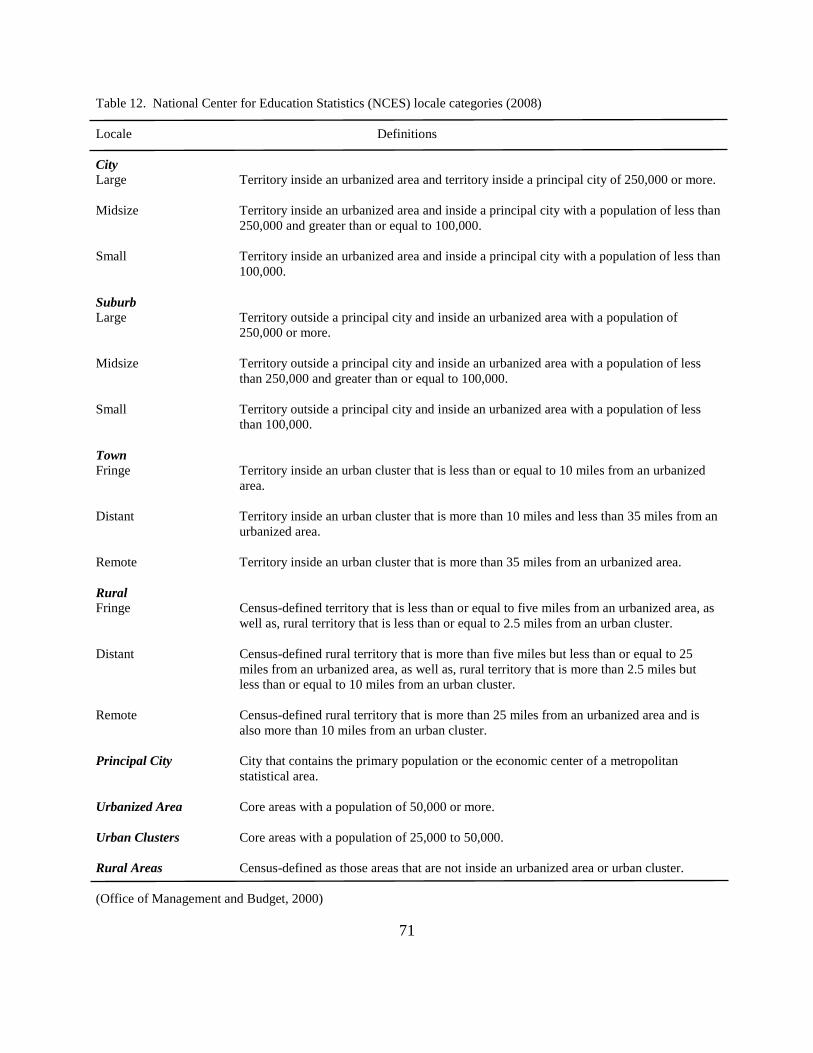
http://dpi.wi.gov/oea/publications.html

71

Table 12. National Center for Education Statistics (NCES) locale categories (2008)

Locale Definitions

City

Large Territory inside an urbanized area and territory inside a principal city of 250,000 or more.

Midsize Territory inside an urbanized area and inside a principal city with a population of less than

250,000 and greater than or equal to 100,000.

Small Territory inside an urbanized area and inside a principal city with a population of less than

100,000.

Suburb Large Territory outside a principal city and inside an urbanized area with a population of

250,000 or more.

Midsize Territory outside a principal city and inside an urbanized area with a population of less

than 250,000 and greater than or equal to 100,000.

Small Territory outside a principal city and inside an urbanized area with a population of less

than 100,000.

Town Fringe Territory inside an urban cluster that is less than or equal to 10 miles from an urbanized

area.

Distant Territory inside an urban cluster that is more than 10 miles and less than 35 miles from an

urbanized area.

Remote Territory inside an urban cluster that is more than 35 miles from an urbanized area.

Rural Fringe Census-defined territory that is less than or equal to five miles from an urbanized area, as

well as, rural territory that is less than or equal to 2.5 miles from an urban cluster.

Distant Census-defined rural territory that is more than five miles but less than or equal to 25

miles from an urbanized area, as well as, rural territory that is more than 2.5 miles but

less than or equal to 10 miles from an urban cluster.

Remote Census-defined rural territory that is more than 25 miles from an urbanized area and is

also more than 10 miles from an urban cluster.

Principal City City that contains the primary population or the economic center of a metropolitan

statistical area.

Urbanized Area Core areas with a population of 50,000 or more.

Urban Clusters Core areas with a population of 25,000 to 50,000.

Rural Areas Census-defined as those areas that are not inside an urbanized area or urban cluster.

(Office of Management and Budget, 2000)

72

NCES categorizes schools using the geographic coordinates of the location, supplemented by

aerial photographs. This procedure sometimes results in classifications that are clearly

inaccurate. For example, Racine Case High School is classified as “rural.” NCES staff

explained that the aerial photography shows that the school is bordered on one side by city, but

on the other side by undeveloped land (F. Johnson, NCES staff member, personal

communication, January 18, 2012). This led to the classification of the school as “rural,” but

clearly, it is a part of the Racine Unified School District, and the students are from Racine. This

same problem led to a rural classification for twelve other high schools that are clearly not rural.

These high schools enroll more than 1,000 students and are located within or close to larger

cities. The source of the error is that NCES geographically defines these high schools as rural

based on their physical address, which is on the edge of towns or cities and connected to an

underdeveloped area. Therefore, the researcher reclassified the following 13 high schools from

the NCES “rural” category into a more appropriate geographical category listed in Table 13.

73

Table 13. Geographical reclassification of 13 rural high schools

Name of High

School

Population of

Students

2009-2010

City Location Census

Population

2010

Name of

Nearest City

& Population

2010

Miles to

Nearest

City

New

Geographical

Classification

Ashwaubenon 1,048 Ashwaubenon 16,693 Green Bay:

104,057

4.15 Suburb

Racine Case 1,984 Racine 78,860 Racine:

78,860

5.27 City

Westosha

Central

1,201 Salem 12,067 Kenosha:

99,218

15.59 Town

Wausau East 1,195 Wausau 39,106 Wausau:

39,106

2.74 City

Hamilton 1,348 Sussex 10,518 Milwaukee:

594,833

20.54 Town

Hortonville 1,118 Hortonville 2,711 Appleton:

76,623

13.90 Town

Kaukauna 1,184 Kaukauna 15,462 Appleton:

72,623

7.97 Suburb

Merrill 1,109 Merrill 9,661 Wausau:

39,106

23.75 Town

Muskego 1,761 Muskego 24,135 Milwaukee:

594,833

18.5 Suburb

Neenah 2,124 Neenah 25,501 Appleton:

72,623

9.34 Suburb

New Berlin 1,164 New Berlin 39,584 Milwaukee:

594,833

14.07 Suburb

Oregon 1,154 Oregon 9,231 Madison:

233,209

11.20 Suburb

Wilmot Union 1,158 Salem 12,067 Kenosha:

99,218

16.94 Town

As the NCES (U.S. Department of Education, 2008) geographical definitions stated on

pages 69-70, a city locale is defined by as territory inside an urbanized area and inside a principal

city with a population of less than 100,000 to greater than 250,000. As Table 13 illustrates,

Racine Case High School is located within the city limits of Racine with a population of 78,860

according to the U.S. Census Bureau (2011) and was reclassified under the city category.

Wausau East is located in the city of Wausau with a population of 39,106 (U.S. Census Bureau,

2011). Its counterpart Wausau West, located on the other side of town, was defined as city

according to NCES. For these two reasons, Wausau East was also reclassified as a city school.

74

NCES (U.S. Department of Education, 2008) also defined a suburb as a territory outside

a principal city and inside an urbanized area with a population of less than 100,000 to greater

than 250,000. These high schools, formerly defined as rural were reclassified as suburb:

Ashwaubenon, Kaukauna, Muskego, Neenah, New Berlin and Oregon.

Lastly, NCES (U.S. Department of Education, 2008) defined a town as territory inside an

urban cluster that is less than or equal to 10 miles to 35 miles from an urbanized area. Five high

schools were reclassified as town schools: Westosha, Hamilton, Hortonville, Merrill and Wilmot

Union. The researcher felt the reclassifications were a better representation of the actual

geographical location in which the schools reside.

Socioeconomic Status (SES)

The SES percentage was defined as the total number of high school students who

participated in the Free and Reduced-Price Lunch (FRPL) program provided by NCES Common

Core Data for Public Schools divided by the total enrollment provided WDPI for the 2009-2010

school year. FRPL provides a proxy measure for the number of low-income students within the

school and is widely used in educational research as such (Hopkins, 2005; Howley, 1989).

NCES defines FRPL as the number of students who are eligible for free and reduced lunch under

the National School Lunch Act, which provides monetary subsidies based on a families’ size and

income level. The federal guidelines for FRPL in 2009-2010 are presented in Table 14.

75

Table 14. Income Eligibility Guidelines

Household Size Federal Poverty Guidelines

1 $10,830

2 $14,570

3 $18,310

4 $22,050

5 $25,790

6 $29,530

7 $33,270

8 $37,010

For each additional family

member, add $3,740

(U.S. Department of Agriculture, 2011)

Through WDPI and NCES, some rural high schools in Wisconsin were classified

specifically as 9-12, 7-12, 6-12 and Kindergarten through 12. By doing so, free and reduced

lunch participation data for each of these schools was inaccurate. After further research, it was

found that NCES only posts the data that is provided to it by WDPI. After contacting a staff

member at WDPI about acquiring data specifically for grades 9-12, it was stated that the online

resources did not include free and reduced lunch participation data specifically by grade level.

After further research, it was not intuitive as to which high schools included other grade level

data. Therefore, each high school was individually researched to see if other grade level data

were included. After researching all 417 high schools, it was concluded that 104 schools’ free

and reduced lunch participation data could not be delineated by grade level to include only

grades 9-12. Information on this variable was left blank for 104 high schools listed in Appendix

A.

Although the FPRL is an established indicator of students living in poverty, it does have

its limitations. First, not all students who qualify for FPRL enroll in the program. Second, each

school district has a different way of promoting the FPRL through announcements, mailings,

76

websites, student registration, and other activities. Nevertheless, some families may not have

been aware of the FPRL program. Consequently, the percent FPRL is not a perfect proxy for the

percent of school families living in poverty. However, it is reasonably accurate in measuring

large variations and is by far the best data available. Thus, it was the most reliable construct for

this study.

Students of Color

Previous studies cited in the literature review have shown achievement gaps, specifically

in southeast Wisconsin, concerning the Black student population. Students of color have been

established as a factor when discussing academic achievement. The WINSS data collection

system was used to identify the following five categories of race/ethnicity: 1) American Indian,

2) Asian, 3) Black, 4) Hispanic and 5) White for the 2009-2010 school year. Because the data

were from 2009-2010, WDPI only collected data within these five categories based on the

previous federal reporting guidelines, and each student was identified by one category only. The

five categories are defined as follows by the U.S. Department of Education (2008):

American Indian - a person with origins in any of the original peoples in North, Central

and South America, who maintains tribal affiliations or community attachment.

Asian – a person having origins in any of the original peoples of the far East, Southeast

Asia, or the Indian subcontinent including Cambodia, China, India, Japan, Korea,

Malaysia, Pakistan, the Philippine Islands, Thailand and Vietnam.

Black – a person having origins in any of the black racial groups of Africa.

Hispanic – a person of Cuban, Mexican, Puerto Rican, South or Central America or other

Spanish culture or origin.

77

White – A person having origins in any of the original peoples of Europe, the Middle

East or North Africa.

The Public Enrollment Master (PEM10.xls) provided the grade level data by gender and

ethnicity/race within each individual high school. Enrollment is based on the third Friday count

in September (WDPI, 2012). The students of color percentage was calculated by the sum of the

total number of students in the American Indian, Asian, Black and Hispanic categories divided

by the total high school enrollment.

Limitations to this data included the new classification system that designated two

additional categories implemented in the 2010-2011 school year. WDPI has now included a

two-part question format that will now allow for the collection of individuals of two or more

races (WDPI, 2011). To stay consistent with the timeline of this study, data from the WINSS

database provided for the 2009-2010 school year was used.

Spending per Pupil

The WDPI has a School Data Warehouse that contains reports such as the comparative

cost and revenue per member, equalized aid and value per member, mill rates, etc. For the

purposes of this study, spending per pupil was defined by total district cost per member. The

total district cost per member is the sum of the total educational cost per member (i.e.

instructional, pupil/staff support and operations/administration), transportation cost per member,

facility cost per member and the food and community services cost per member. The WDPI and

the Wisconsin Association of School Business Officials (WASBO) jointly developed this cost

methodology. In 2009-2010, the state average for spending per pupil was $12,624, comprised of

educational costs ($10,836 or 86%), transportation costs ($475 or 4%), facility costs ($775 or

78

6%) and food and community services costs ($537 or 4%). These data were also reported on

WINSS and extracted from the database for this study.

High School Enrollment

The WDPI collects enrollment data as a part of the Individual Student Enrollment System

(ISES) based on the Wisconsin Student Number Locator System (WSLS) and reported on the

third Friday of September each academic school year. The Public Enrollment by District by

School by Grade (PESGr10.xls) was used for the total enrollment for grades 9-12 in all public

high schools in Wisconsin. These data reflected enrollment by grade, by school and school

district reported on the third Friday in September of each academic school year (WDPI, 2012).

Parent Education Level

As the literature review indicated, parent education level can have a positive impact on a

child’s academic achievement. However, the average parent education level by school or by

school district is not a measure that is collected in the state of Wisconsin. Therefore, average

income per school district has been chosen as a surrogate variable to represent parent education

level. According to the U. S. Census Bureau (2011), the Current Population Survey

demonstrates the higher the educational attainment, the more earnings an individual would have

over a lifetime, thus providing a numerical measure for parent education level.

This survey has been in existence for more than 50 years and is given monthly to 50,000

households done by the Bureau of Census for the Bureau of Labor Statistics. The survey collects

data regarding employment, unemployment, earnings, hours of work, etc.

The median annual earnings by educational attainment are illustrated in Figure 1.

79

Figure 1. Median Annual Earnings by Educational Attainment (in 2008 dollars)

United States Department of Labor (2011)

For example, an individual who does not graduate high school has an annual median

income of $17,569 versus an individual with a professional degree with an annual median

income of $83,304. Research indicated that a parent’s educational level is highly correlated with

a child’s educational attainment, and educational attainment is highly correlated with household.

Thus, average household income in the school district is a reasonable proxy for family education

level.

However, there are limitations in using this variable. Individual income and education

level are not perfectly correlated – some individuals with little education have high income, and

$0

$10,000

$20,000

$30,000

$40,000

$50,000

$60,000

$70,000

$80,000

$90,000

80

some individuals who are highly educated have low income. In addition, according to the

Wisconsin Department of Revenue (2011), only individuals who have designated the school

district they live in on their tax returns are included in this data. Also, this measure does not

include individuals who do not file tax returns because their income falls below the minimum-

filing requirement that would lead to an overestimate of average household income. This

potentially serious omission is partially corrected by including in the model the percentage of

students receiving free and reduced lunch. The variable excludes other sources of income that

are fully or partially exempt from taxes such as social security, public assistance or

unemployment compensation which would lead to an underestimate of average household

income. Lastly, this measure does also not include income from nonresident property owners or

corporations located within the school districts, but these omissions are not tied to school district

residents.

Truancy

WDPI (2011) defines truancy as a student who is absent from school without an

acceptable excuse for part or all of five or more days each semester. Truancy is calculated by

dividing the total number of truants in grades 9-12 by the total high school enrollment and is

expressed as a percentage. However, certain high school data were reported as grades 6-12, 7-12

and KG-12. High schools’ (Appendix B) data were modified to only include 9-12 truancy data

based on grade level delineation provided by WINSS (WDPI, 2012).

A limitation to this construct was that it is often at the school administrator’s discretion

when a student is referred for truancy although there was no data to represent this variance. A

total of 10 days per school year is stated within the statute; however, it may be several more days

81

before a student is referred for truancy based on the individual circumstances. Another limitation

to this variable was that the data is self-reported by each high school and subject to individual

interpretation of definitions for reporting purposes.

Disciplinary Actions: Suspensions and Expulsions

According to WDPI (2011), out-of-school suspensions and expulsions are used as

measures of disciplinary actions. Wisconsin State Statute 120.13(1) defines out-of-school

suspension (b) as “absences from school imposed by the school administration for

noncompliance with school district policies or rules, for threatening to destroy school property,

or for endangering the property, health, or safety of those at school.” Expulsions are defined as

“absences from school for purposes of discipline as imposed by the school board for violation of

school district rules; threats against school property; or conduct which endangers the property,

health, or safety of those at school.” Expulsion is a school board action defined by Wisconsin

State Statute 120.13(1) (c) and 119.25 (WDPI, 2011).

The total percentage of students with disciplinary action was the sum of the total number

of pupils suspended out-of-school in grades 9-12 and the total number of pupils expelled in

grades 9-12 as reported by WINSS for the 2009-2010 academic school year divided by the high

school enrollment. However, certain high school data were reported as grades 6-12, 7-12 and

KG-12. High schools’ (Appendix B) data were modified to include only 9-12 suspension and

expulsion data based on grade level delineation provided by WINSS (WDPI, 2012).

Limitations to this variable were that the data is self-reported by each high school and

subject to individual interpretation of definitions for reporting purposes and can be skewed based

82

on one event. The out-of-school and expulsion data were extracted from the WINSS database

for the 2009-2010 academic school year.


WDPI (2011) follows the Wisconsin Administrative Cody, Section PI 11.36 for special

education eligibility for the following disabilities: autism, cognitive disabilities, emotional

behavioral disabilities, hearing impairments, orthopedic impairment, other health impairment,

significant development delay, speech/language impairments, specific learning disabilities,

traumatic brain injury, and visual impairments. Program consultants have developed eligibility

criteria worksheets to aid in determining if a student qualifies for special education services.

Students who are identified and have an individual education plan (IEP) will be counted as a part

of the students with disabilities construct.

The students with disabilities percentage was the total number of students diagnosed with

a disability within grades 9-12 divided by high school enrollment. Through WDPI and NCES,

some rural high schools in Wisconsin were classified specifically as 9-12, 7-12, 6-12 and

Kindergarten through 12. By doing so, students with disabilities percentages for each of these

schools were inaccurate. After further research, it found that NCES only posted the data that was

provided to it by WDPI. After contacting a staff member at WDPI about acquiring data

specifically for grades 9-12, it was stated that the online resources did not include students with

disabilities data specifically by grade level. After further research, it was not intuitive as to

which high schools included other grade level data. Therefore, each high school was

individually researched to see if other grade level data were included. After researching all 417

high schools, it was concluded that 104 high schools’ students with disabilities data could not be

83

delineated by grade level to only include grades 9-12 and, therefore, data on this variable for the

high schools listed in Appendix A was left blank.


Extra/Co-curricular activity participation is defined as “school-sanctioned activities

intended to broaden, develop, and enhance a student’s school experience in the areas of

academics, athletics, and music. Participation is not required and the group or event is not

offered for credit or grade” (WDPI, 2005, p. 18). A limitation to this variable was that the data

were self-reported by each high school and subject to individual interpretation of definitions for

reporting purposes. The extra/co-curricular participation index was the sum of the percentage of

pupils participating in grades 6-12 academic, athletic and music extra/co-curricular activities as

reported by WINSS for the 2009-2010 academic school year. In all cases, the data were reported

at the 6-12 level; separate 9-12 data were not available. Some students may participate in

academic, athletic and music extra/co-curricular activities, so percentages may be represented in

numbers greater than 100%.

Data Analysis

In the state of Wisconsin, there are 417 traditional public high schools. Of those, 229 are

located in rural areas (54.9%); 82 are located in towns (19.7%); 61 are located in suburban areas

(14.6%) and 45 are city schools (10.8%) (U.S. Department of Education, 2011). Only data from

traditional public high schools were included in this study. Certain nontraditional high schools

have been excluded including parochial, alternative, charter, magnet, single purpose schools and

juvenile detention centers.

84

For each data source, the data were downloaded to an Excel® spreadsheet. The data were

then uploaded into the SPSS software which was used in the statistical analysis. The key result of

most interest was the size and significance of the coefficient on the Geography variable.

In closing, although no variable is perfect, it was reasonable to assume that each of the

ten variables or their surrogate were statistically sound.

Human Participants Review Board (HPRB) Approval

The HPRB process does not apply to this study due to the use of public data sources of an

aggregate nature such as data by community, school district, county, etc. There were no human

subjects within this study; therefore, there was no risk to anyone individually.

Summary

In Chapter 3, the research methodology was presented including the research design and

the conceptual model. The limitation of regression and aggregation bias was explained and

acknowledged. Descriptions of the data sources were provided along with specific data

definitions for all ten independent variables and five dependent variables. The method of

analysis was also defined. In Chapter 4, the results of implementing this methodology will be

fully presented.

85

CHAPTER 4

RESULTS

The purpose of this study was to distinguish how rural Wisconsin high students

performed on the tenth grade WKCE in the areas of reading, language arts, mathematics, science

and social studies compared to Wisconsin city, suburb and town public high students.

The most fundamental problem with the use of multiple regressions to analyze the

determinants of academic achievement by high school was the possibility of aggregation bias

and the ecological fallacy. Students take exams, not schools; therefore, it was possible that using

aggregate data would produce results different from the results using individual data. Although

other research demonstrated that the probability of these problems was low, it was not zero. As

the data discussion that follows will show, the results in the aggregate data paralleled very

closely the research based on data from individual student performance, so the ecological fallacy

was not a problem in this study.

86

DATA DESCRIPTIONS

Prior to analyzing the relationships among the variables, each variable was described in

statistical terms including the mean and standard deviation. WKCE test scores in the areas of

Reading, Language Arts, Mathematics, Science and Social Studies represented the dependent

variable of high school academic achievement. The independent variables were described in

detail in Chapter 3 and included the following: geographic location, the percentage of students

receiving free and reduced lunch (SES), the percentage of students of color in the high school

enrollment, spending per pupil in the school district, high school enrollment, average income in

the school district (parent education level), truancy cases as a percent of enrollment, total

suspensions and expulsions as a percent of the enrollment, the percentage of students with

disabilities and the sum of participation rates in three categories of extra/co-curricular activities.

Academic Achievement

Academic achievement was represented by students who scored proficient or advanced

on the tenth grade WKCE tests in the areas of Reading (Read), Language Arts (LA),

Mathematics (Math), Science (Science) and Social Studies (SS) during the 2009-2010 academic

year. For the purpose of this study, 417 public high schools in Wisconsin data were analyzed,

five including one suburb, and four rural of which did not provide any WKCE test data. Thus

the test data represented 412 schools in each subject area. Table 15 summarizes the WKCE data

for Wisconsin tenth grade students for the 412 high schools for which data was available.

87

Table 15. WKCE Descriptive Statistics

N Minimum Maximum Mean Std. Deviation

Read_ProfAdv 412 18.48 100.00 80.2704 10.78030

LA_ProfAdv 412 13.76 100.00 72.3927 11.86981

Math_ProfAdv 412 10.20 100.00 74.3819 12.56704

Science_ProfAdv 412 9.39 100.00 77.0097 12.31278

SS_ProfAdv 412 12.52 100.00 78.9809 11.36912

Valid N

(list wise)

412

In reading, the percentage of students who scored proficient or advanced included a

minimum of 18.48% students from one city high school to a maximum score of 100.00%

represented by three rural high schools. The average percentage of students who scored

proficient or advanced was 80.27% with a standard deviation of 10.78 percentage points.

In language arts, only 13.76% of students from one city high school scored proficient or

advanced while two rural high schools had 100.00% of students scoring in those categories. The

average percentage of students scoring proficient or advanced was 72.39% with a standard

deviation of 11.87 percentage points.

In mathematics, only 10.20% of students from one city high school scored proficient and

advanced while 100.00% of students from one rural high school scored within the same range.

The mean percentage of students scoring proficient or advanced was 74.38% with a standard


In science, scoring proficient or advanced included a minimum of 9.39% of students from

one city high school to 100.00% of students from three rural high schools. The average

percentage of students scoring proficient or advanced in science was 77.01% with a standard


88

Lastly, in social studies a minimum of 12.52% of students from one city high school and

a maximum of 100.00% of students from four rural high schools scored in the proficient or

advanced range. The average percentage of students who scored proficient or advanced was

78.98% with a standard deviation of 11.37 percentage points.

Geographic Location

Each school district was classified by NCES as rural, town, suburb or city. This study

included 417 public high schools in the state of Wisconsin. Geographical location data are


Table 16. Geographical Location Descriptive Statistics

Frequency Percent Valid Percent

Cumulative

Percent

Valid City 45 10.8 10.8 10.8

Rural 229 54.9 54.9 65.7

Suburb 61 14.6 14.6 80.3

Town 82 19.7 19.7 100.0

Total 417 100.0 100.0

Of those, 45 high schools are designated as city; 229 are located in rural areas; 61 are in

suburbs, and 82 are in towns. Thus, a high school in a city represents 10.8% of the total number

of schools while rural, suburb and town high schools represent 54.9%, 14.6% and 19.7%

respectively, the same proportions as discussed in Chapter 1.

Free and Reduced Lunch (SES)

Socioeconomic status was represented by the percentage of free and reduced lunch

participants within the high school. Although there are 417 high schools, data were available for

only 313 high schools for this variable. Data for the other 104 high schools contained other

89

grade level data (i.e. 6-12, 7-12, middle/high, etc.) that could not be separated out. Attempts to

obtain high school free and reduced lunch participation data from NCES, WDPI WINSS and the

National School Lunch program were unsuccessful and, therefore, data for this variable for those

104 high schools were not included in this study. These 104 high schools listed in Appendix A

included 89 rural, eight town, five suburb and two city high schools. The data for free and

reduced lunch are summarized in Table 17.

Table 17. Free and Reduced Lunch Descriptive Statistics


FRRL_Per 313 .56 86.03 30.0190 15.57029

Valid N (list wise) 313

One suburban high school had the lowest percentage of students who participated in free

and reduced lunch at .56% while one city high school had the highest rate of participation at

86.03%. The average percentage of students participating in free and reduced lunch in

Wisconsin high schools was 30.02% with a standard deviation of 15.57 percentage points. An

analysis of the scatter plot (see Appendix C) revealed a cluster of six schools, all city schools,

that had more than 77% of its students participating in the free or reduced lunch program and lay

substantially outside the distribution of the other observations. These outliers were analyzed later

to determine whether they influenced the findings of the study. The results of this analysis will

be reported under the regression analysis.

Students of Color

Students of color in a high school was measured by the percentage of students within four

ethnicity categories including Asian, Black, Hispanic and American Indian as defined by WDPI.

These data are summarized in Table 18.

90

Table 18. Students of Color Descriptive Statistics


Students_Color_Per 417 .0000 99.3266 12.770983 18.1375102


Of the 417 high schools, there were five rural high schools that had no students of color.

Conversely, the maximum percentage of students of color was 99.33% at one rural high school.

The average percentage of students of color in a high school was 12.77% with a standard

deviation of 18.14 percentage points. A scatter plot (see Appendix C) analysis revealed a cluster

of ten schools, nine city and one rural high school, that had more than 85% students of color and

that lay substantially outside the distribution for the other observations. These outliers were

analyzed later to determine whether they influenced the findings of the study. The results of this

analysis will be reported under the regression analysis.

Spending per Pupil

Spending per pupil per school district was provided by WDPI and represented the total

district cost per member which is the sum of the total educational cost per member (i.e.

instructional, pupil/staff support and operations/administration), transportation costs per member,

facility costs per member and the food and community services cost per member. The variable is

expressed in thousands of dollars of income. Per pupil spending data are summarized in Table

19.

91

Table 19. Spending per Pupil ($’000) Descriptive Statistics


Spend_Pupil 417 4.107 24.377 12.90544 1.752995


The minimum spending per pupil per school district was $4,107 in one rural school

district while the maximum was $24,377 in one rural school district. The average spending per

pupil per school district was $12,905 with a standard deviation of $1,753. A scatter plot (see

Appendix C) analysis revealed that all schools were loosely clustered together, and none lay

substantially outside the distribution of the other observations. Therefore, outliers in spending

per pupil were not a concern in the regression analysis.

High School Enrollment (School Size)

High school enrollment was based on the third Friday count in September provided by

the WDPI and is summarized in Table 20.

Table 20. High School Enrollment Descriptive Statistics


Enrollment 417 24 2408 625.49 545.448


Of the 417 public high schools, the lowest enrollment during the 2009-2010 academic

school year was at one rural high school with 24 students. One suburban high school had the

highest enrollment with 2,408 students. The average number of students attending a high school

in Wisconsin was 625 with a standard deviation of 545 students. A scatter plot (see Appendix C)

analysis revealed that all schools were loosely clustered together, and none were substantially

92

outside the distribution for the other observations. Therefore, outliers in the high school size

variable were not a concern in the regression analysis.

Average Income by School District (Parent Education Level)

Parent education level was measured by the surrogate variable of average income per

school district as provided by the WDOR. The unit of measure for the variable was thousands of

dollars of income. These data are summarized in Table 21.

Table 21. Average Income per School District ($’000) Descriptive Statistics


Avg_Inc_SD 417 5.344 65.748 31.58667 7.072919


Of the 417 high schools, one rural school district had the lowest average income per

school district at $5,344; however, one suburban school district had the highest with $65,748.

The average income per school district in the state of Wisconsin was $31,587 with a standard

deviation of $7,073. A scatter plot (see Appendix C) analysis revealed that all schools were

loosely clustered together, and none lay substantially outside the distribution of the other

observations. Therefore, outliers in the average income by school district variable were not a

concern in the regression analysis.

Truancy

The truancy rate was defined as the number of students who were absent without an

acceptable excuse for part or all of five or more days each semester as defined by the WDPI

divided by the school enrollment as defined by the WDPI. The truancy rate can be greater than

100% as a single student can be identified as truant multiple times throughout a school year.

93

Truancy data are summarized in Table 22.

Table 22. Truancy Descriptive Statistics


Truancy_Per 417 .00 111.08 8.5809 15.34163


Of the 417 high schools in Wisconsin, twenty-nine high schools reported as having zero

students truant during the 2009-2010 school year including twenty-eight rural high schools and

one town high school. The high school with the highest truancy rate was a city high school at

111.08%. The average truancy rate within a Wisconsin public high school was 8.58% with a

standard deviation of 15.34 percentage points. A scatter plot (see Appendix C) analysis revealed

a cluster of nine schools, eight city and one rural high school, that had a truancy rate of more

than 70% and lay substantially outside the distribution for the other observations. These outliers

were analyzed later to determine whether they influenced the regression findings, and the results

will be reported in the regression analysis section.

Disciplinary Actions: Suspensions and Expulsions

Disciplinary actions were defined as the number of suspensions plus the number of

expulsions divided by the school enrollment, all as defined by WDPI. The data were obtained

through the WINSS database, and again a single student may have multiple cases of suspension

or expulsion during the school year. Disciplinary action data are summarized in Table 23.

Table 23. Disciplinary Actions: Suspensions & Expulsions Descriptive Statistics


Sum_Sus_Exp 417 .00 94.21 6.6150 9.74703


94

Out of the 417 high schools, eight reported having zero out-of-school suspensions or

expulsions for the 2009-2010 school year. All eight were rural high schools. The high school

reporting the most out-of-school suspensions and expulsions was one city high school at 94.21%.

The mean out-of-school suspension and expulsions rate was 6.62% with a standard deviation of

9.75 percentage points. A scatter plot (see Appendix C) analysis revealed a cluster of eight

schools, all city schools that had a combined suspension and expulsion rate of more than 40%

and lay substantially outside the distribution of the other observations. These outliers were

analyzed later to determine whether they influenced the findings of the study. The results of this

analysis will be reported under the regression analysis section.


Students with disabilities were represented by the percentage of students diagnosed with

a disability within the high school. Although there are 417 high schools, data were available for

only 313 high schools because data for the other 104 high schools listed in Appendix A including

89 rural, eight town, five suburb and two city contained other grade level data (i.e. 6-12, 7-12,

middle/high, etc.) that could not be separated or disaggregated to only include grades 9-12.

Attempts to obtain students with disabilities high school data from NCES, WDPI WINSS and the

WDPI special education department were unsuccessful and, therefore, data for this variable for

those 104 high schools were not included in this study. Data for the 313 high schools are


Table 24. Students with Disabilities Descriptive Statistics


Stud_Dis_Per 313 5.44 64.23 13.6945 4.71350


95

From the 313 high schools in Wisconsin, a town high school had the lowest percentage of

students with disabilities at 5.44% while a city high school had the highest rate at 64.23%. The

average percentage of students with disabilities in a Wisconsin high school was 13.69% with a

standard deviation of 4.71 percentage points. An analysis of the scatter plot (see Appendix C)

revealed that one city school had more than 60% of its students identified as having a disability.

This observation lay substantially outside the distribution of all of the other observations and was

analyzed later to determine whether it influenced the findings of the study. The results of this

analysis will be reported under the regression analysis.


Extra/co-curricular activities were represented by the sum of the percentages of students

who participated in academic, athletic and music school sanctioned activities as defined by the

WDPI. The extra/co-curricular activities index can be greater than 100% as a single student may

participate in multiple activities throughout the school year. These data are summarized in Table

25.

Table 25. Extra/Co-curricular Participation Index Descriptive Statistics


Extra_Total 417 .00 277.62 119.0947 43.49348


Out of the 417 high schools in Wisconsin, twelve schools reported offering no extra/co-

curricular activities within the high school including eleven city high schools and one rural high

school. A rural high school had the highest participation rate at 277.62%. The average

participation rate was 119.09% with a standard deviation of 43.49 percentage points. An

analysis of the scatter plot (see Appendix C) revealed that all schools were loosely clustered

96

together, and none lay substantially outside the distribution of the other observations. Therefore,

outliers in the extra/co-curricular activities participation variable were not a concern in the

regression analysis.

DATA CORRELATIONS

The data correlation matrix included all variables including dependent and independent

and represents the relationship between the pairs of variables. The Pearson correlation

coefficient (r) ranges from -1.00 to +1.00 and the strength of the relationship is indicated by the

absolute value of the coefficient. In this section, the discussion of correlation was based on the

bivariate correlation coefficient, the simple correlation between two variables. In the regression

analysis, partial correlation coefficients were used to analyze potential problems with

multicollinearity. The partial correlation coefficient was the correlation between two variables,

controlling for the effects of other variables, and in particular those variables included in the

regression analysis. The total or bivariate correlation coefficient was analogous to the total

derivative, and the partial correlation coefficient is analogous to the partial derivative. In

general, the partial correlation coefficient will differ from the bivariate correlation coefficient.

Only data correlations greater than .500 (positive and negative) were included in this

discussion. Many other correlations are statistically significant (i.e. different from zero at the .05

level of probability), but the strength of the association is relatively weak. Again, a low bivariate

correlation coefficient does not necessarily imply a low partial correlation coefficient when

controlling for the influence of the other variable. The correlations involving the dependent

variables of Reading, Language Arts, Mathematics, Science and Social Studies will be discussed

in detail in the data regression section. In the bivariate correlations, the number of observations

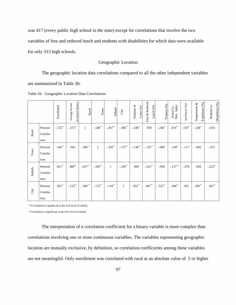
97

was 417 (every public high school in the state) except for correlations that involve the two

variables of free and reduced lunch and students with disabilities for which data were available

for only 313 high schools.

Geographic Location

The geographic location data correlations compared to all the other independent variables

are summarized in Table 26.

Table 26. Geographic Location Data Correlations

En

roll

men

t

Av

erag

e In

com

e

by

Sch

oo

l D

istr

ict

Ru

ral

To

wn

Su

bu

rb

Cit

y

Stu

den

ts o

f

Colo

r (%

)

Fre

e &

Red

uce

d

Lun

ch (

%)

Tru

ancy

(%

)

Ex

tra/

Co

-

Par

t. In

dex

Spen

din

g p

er P

upil

Su

spen

sio

ns

&

Exp

uls

ion

s (%

)

Stu

den

ts w

/

Dis

abil

itie

s (%

)

Ru

ral

Pearson

Correla-

tion

-.722** -.273** 1 -.546** -.457** -.384** -.349** .050 -.246** .474** .159** -.236** -.016

To

wn Pearson

Correla-

tion

.144** .045 -.546** 1 -.205** -.172** -.136** -.155** -.096* -.109* -.172** -.092 -.072

Su

bu

rb Pearson

Correla-

tion

.411** .468** -.457** -.205** 1 -.144** .069 -.312** -.004 -.137** -.076 -.002 -.223**

Cit

y

Pearson

Correla-

tion

.505** -.153** -.384** -.172** -.144** 1 .655** .467** .523** -.466** .051 .500** .361**

**Correlation is significant at the 0.01 level (2-tailed).

*Correlation is significant at the 0.05 level (2-tailed).

The interpretation of a correlation coefficient for a binary variable is more complex than

correlations involving one or more continuous variables. The variables representing geographic

location are mutually exclusive, by definition, so correlation coefficients among these variables

are not meaningful. Only enrollment was correlated with rural at an absolute value of .5 or higher

98

(r = -.722, r2

= .52). No variables were highly correlated with Town or Suburb. City was highly

correlated with four variables: 1) enrollment (r = .505, r2

= .26), 2) students of color (r = .655, r2

= .43), 3) truancy (r = .523, r2

= .27) and 4) suspensions and expulsions (r = .500, r2

= .25).

Therefore, 26% of the variation of city is explained by enrollment, 43% by students of color,

27% by truancy and 25% by suspensions and expulsions respectively. Overall:

The higher the enrollment, the more likely the school will be located in a city.

The higher the percentage of students of color, the more likely the school is located in a

city.

The higher the truancy rate, the more likely the school is in a city.

The higher the suspension and expulsion rates, the more likely the school is in a city.

These results are consistent with previous studies in the literature regarding geographic location.

Free and Reduced Lunch

The free and reduced lunch data correlations compared to all the other independent

variables are summarized in Table 27.

Table 27. Free and Reduced Lunch Data Correlations

En

roll

men

t

Av

erag

e In

com

e

by S

chool

Dis

tric

t

Ru

ral

To

wn

Su

bu

rb

Cit

y

Stu

den

ts o

f

Colo

r (%

)

Tru

ancy

(%

)

Ex

tra/

Co

-

curr

icu

lar

Ind

ex

Sp

end

ing

per

Pu

pil

Su

spen

sio

ns

&

Exp

uls

ion

s (%

)

Stu

den

ts w

/

Dis

abil

itie

s (%

)

Fre

e &

Red

uce

d

Lunch

(%

) Pearson

Correla-

tion

-.030 -.740** .050 -.155** -.312** .467** .636** .626** -.306** .372** .613** .592**



The free and reduced lunch (FRRL_Per) participation percentage is highly correlated

with five variables including average income by school district, students of color, truancy,

99

suspensions and expulsions and students with disabilities. As will be discussed in the next

section, these numerous high correlations created multicollinearity problems in the regression

analysis. These data are summarized in Table 28.

Table 28. Free and Reduced Lunch Pearson (r) Correlations

Variable Pearson Correlation (r) r2

Average Income by School District -.740 .55

Students of Color .636 .40

Truancy .626 .39

Suspensions & Expulsions .613 .38

Students with Disabilities .592 .35

The amount of variation in the free and reduced lunch participation percentage variable

that is associated with variation in the other variables are the following: average income by

school district (55%), students of color (40%), truancy (39%), suspensions and expulsions (38%)

and students with disabilities (35%). Several observations follow from the correlations:

The higher the average income by school district, the lower the participation rate in free

and reduced lunch, and vice versa.

The higher the percentage of students of color, the higher the participation percentage in

free and reduced lunch.

The higher the truancy rate, the higher the free and reduced lunch participation rate.

The higher the suspensions and expulsions percentage, the higher the participation

percentage in free and reduced lunch.

100

The greater the students with disabilities percentage, the higher the participation

percentage in free and reduced lunch.

These findings are consistent with previous research within the literature.

Students of Color

The students of color data correlations compared to all the other independent variables


Table 29. Students of Color Data Correlations

En

roll

men

t

Av

erag

e In

com

e

by S

chool

Dis

tric

t

Ru

ral

To

wn

Su

bu

rb

Cit

y

Fre

e &

Red

uce

d

Lu

nch

(%

)

Tru

ancy

(%

)

Ex

tra/C

o-

curr

icu

lar

Index

Sp

end

ing

per

Pu

pil

Su

spen

sio

ns

&

Exp

uls

ion

s (%

)

Stu

den

ts w

/

Dis

abil

itie

s (%

)

Stu

den

ts o

f

Co

lor

(%)

Pearson

Correla-

tion

.389** -.214** -.349** -.136** .069 .655** .636** .762** -.549** .210** .734** .475**



The student of color (Students_Color_Per) variable was highly correlated with five other

independent variables as shown in Table 30:

Table 30. Students of Color Pearson (r) Correlations


City .655 .43

Free & Reduced Lunch .636 .40

Truancy .762 .58

Extra/Co-curricular -.549 .30

Suspensions & Expulsions .734 .54

101

The proportion of variation in the students of color variable that can be explained by

variation in the other variables are the following: city (43%), free and reduced lunch (40%),

truancy (58%), extra/co-curricular participation (30%) and suspensions and expulsions (54%)

and vice versa. Results included the following observations:

The greater the percentage of students of color, the more likely the school is

located in the city.

The greater the percentage of students of color, the higher the percentage of

students who participated in the free and reduced lunch program.

The greater the percentage of students of color, the higher the truancy rate for that

school.

The greater the percentage of students of color, the lower the extra/co-curricular

participation index.

The greater the percentage of students of color, the higher the sum of the

combined suspension and expulsion rates within that school.

These correlations are consistent with similar results within the literature. This series of high

correlations proved to be troublesome in the regression analysis and will be discussed in the

regression section.

Spending per Pupil

The spending per pupil data correlations compared to all the other independent variables


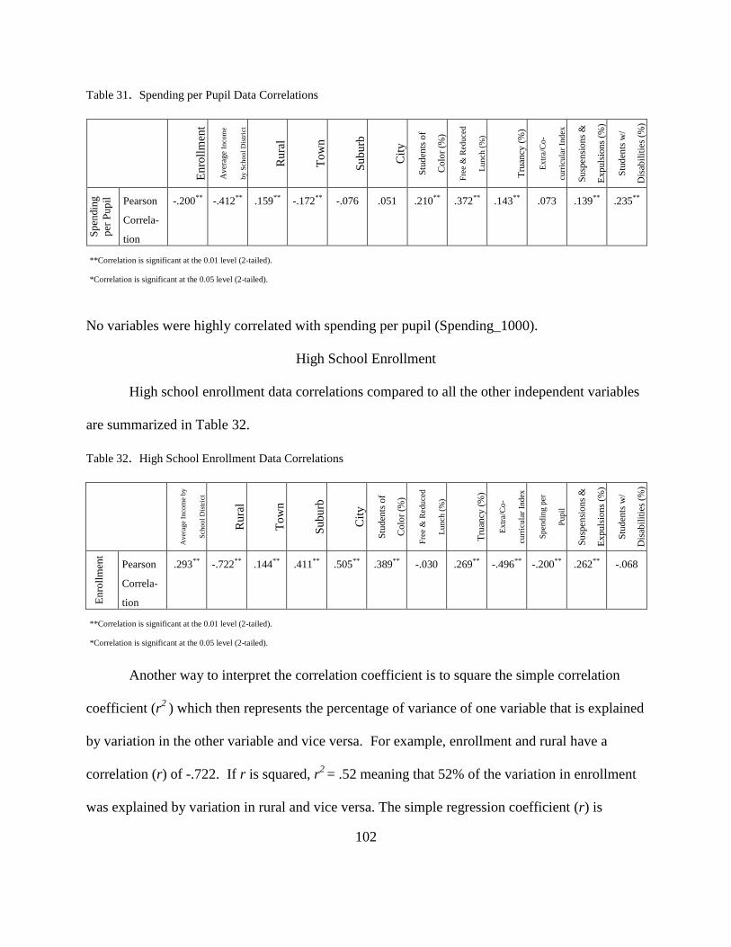
102

Table 31. Spending per Pupil Data Correlations

En

roll

men

t

Aver

age

Inco

me

by S

chool

Dis

tric

t

Ru

ral

To

wn

Su

bu

rb

Cit

y

Stu

den

ts o

f

Colo

r (%

)

Fre

e &

Red

uce

d

Lunch

(%

)

Tru

ancy

(%

)

Extr

a/C

o-

curr

icula

r In

dex

Su

spen

sio

ns

&

Exp

uls

ion

s (%

)

Stu

den

ts w

/

Dis

abil

itie

s (%

)

Sp

endin

g

per

Pup

il

Pearson

Correla-

tion

-.200** -.412** .159** -.172** -.076 .051 .210** .372** .143** .073 .139** .235**



No variables were highly correlated with spending per pupil (Spending_1000).

High School Enrollment

High school enrollment data correlations compared to all the other independent variables


Table 32. High School Enrollment Data Correlations

Aver

age

Inco

me

by

Sch

ool

Dis

tric

t

Ru

ral

To

wn

Su

bu

rb

Cit

y

Stu

den

ts o

f

Colo

r (%

)

Fre

e &

Red

uce

d

Lu

nch

(%

)

Tru

ancy

(%

)

Ex

tra/C

o-

curr

icu

lar

Ind

ex

Sp

end

ing

per

Pu

pil

Su

spen

sio

ns

&

Exp

uls

ion

s (%

)

Stu

den

ts w

/

Dis

abil

itie

s (%

)

En

roll

men

t

Pearson

Correla-

tion

.293** -.722** .144** .411** .505** .389** -.030 .269** -.496** -.200** .262** -.068



Another way to interpret the correlation coefficient is to square the simple correlation

coefficient (r2

) which then represents the percentage of variance of one variable that is explained

by variation in the other variable and vice versa. For example, enrollment and rural have a

correlation (r) of -.722. If r is squared, r2

= .52 meaning that 52% of the variation in enrollment

was explained by variation in rural and vice versa. The simple regression coefficient (r) is

103

negative, meaning that the higher the enrollment, the less likely the school will be rural.

Enrollment is also highly correlated with City (r = .505, r2

= .26) which means 26% of the

variation in enrollment is explained by city and vice versa. Therefore, the higher the enrollment,

the more likely the school will be located in a city. These results are consistent with previous

studies regarding enrollment.

Average Income by School District

Average income by school district data correlations compared to all the other independent


Table 33. Average Income by School District Data Correlations

En

roll

men

t

Ru

ral

To

wn

Su

bu

rb

Cit

y

Stu

den

ts o

f

Colo

r (%

)

Fre

e &

Red

uce

d

Lu

nch

(%

)

Tru

ancy

(%

)

Ex

tra/C

o-

curr

icu

lar

Ind

ex

Sp

end

ing

per

Pu

pil

Su

spen

sio

ns

&

Exp

uls

ion

s (%

)

Stu

den

ts w

/

Dis

abil

itie

s (%

)

Av

g_

Inc_

SD

Pearson

Correla-

tion

.293** -.273** .045 .468** -.153** -.214** -.740** -.266** .012 -.412** -.214** -.420**



Average income by school district (Income_1000) was highly correlated with free and

reduced lunch participation percentage (r = -.740, r2

= .55). Thus, 55% of the variation in

average income by school district could be explained by the variation in free and reduced lunch

participation percentage and vice versa. Since the relationship between the two variables was

negative, the higher the school district average income the lower the free and reduced lunch

participation percentage in the high school. These correlations are consistent with previous

research regarding average income by school district.

104

Truancy

Truancy data correlations compared to all the other independent variables are


Table 34. Truancy Data Correlations

En

roll

men

t

Aver

age

Inco

me

by S

chool

Dis

tric

t

Ru

ral

To

wn

Su

bu

rb

Cit

y

Stu

den

ts o

f

Colo

r (%

)

Fre

e &

Red

uce

d

Lunch

(%

)

Extr

a/C

o-

curr

icula

r In

dex

Spen

din

g p

er

Pupil

Su

spen

sio

ns

&

Exp

uls

ion

s (%

)

Stu

den

ts w

/

Dis

abil

itie

s (%

)

Tru

ancy

(%

)

Pearson

Correla-

tion

.269** -.266** -.246** -.096* -.004 .523** .762** .626** -.463** .143** .760** .542**



Truancy (Truancy_Per) also had five variables that are highly correlated including city, students

of color, free and reduced lunch, suspensions and expulsions and students with disabilities in

Table 35:

Table 35. Truancy Pearson (r) Correlations


City .523 .27


Free and Reduced Lunch .626 .39

Suspensions and Expulsions .760 .58

Students with Disabilities .541 .29

The percentage of the variation in the truancy rate that was explained by variation in the

variables was the following: city (27%), students of color (58%), free and reduced lunch (39%),

105

suspensions and expulsions (58%) and students with disabilities (29%). Therefore, the following

interpretations can be made as follows:

The higher the truancy rate, the more likely the school is within a city.

The higher the truancy rate, the higher the percentage of students of color.

The higher the truancy rate, the higher the participation percentage in free and reduced

lunch.

The higher the truancy rate, the higher the suspensions and expulsions percentage.

The higher the truancy rate, the higher the students with disabilities rate.

These correlations are consistent with other previous research within the literature.

Disciplinary Actions: Suspensions & Expulsions

Disciplinary actions: suspensions and expulsions data correlations compared to all the

other independent variables are summarized in Table 36.

Table 36. Disciplinary Actions: Suspensions & Expulsions Data Correlations

En

roll

men

t

Aver

age

Inco

me

by

Sch

ool

Dis

tric

t

Ru

ral

To

wn

Su

bu

rb

Cit

y

Stu

den

ts o

f

Colo

r (%

)

Fre

e &

Red

uce

d

Lu

nch

(%

)

Tru

ancy

(%

)

Ex

tra/C

o-

curr

icu

lar

Ind

ex

Sp

end

ing

per

Pu

pil

Stu

den

ts w

/

Dis

abil

itie

s (%

)

Su

s &

Exp.

(%)

Pearson

Correla-

tion

.262**

-.214** -.236** -.092 -.002 .500** .734** .613** .760** -.454** .139** .385**



The variable representing the sum of the suspensions and expulsions (Sum_Sus_Exp) rates was

highly correlated with the four variables, city, students of color, free and reduced lunch and

truancy as shown in Table 37.

106

Table 37. Disciplinary Actions: Suspensions & Expulsions Pearson (r) Correlations


City .500 .25


Free & Reduced Lunch .613 .38

Truancy .760 .58

The proportion of variation in the suspension and expulsion variable that is explained by the

other variables was as follows: city (25%), students of color (54%), free and reduced lunch

(38%) and truancy (58%). Thus:

The higher the suspensions and expulsions percentage, the more likely the school is

located in a city.

The higher the suspensions and expulsions percentage, the higher the students of color

percentage.

The higher the suspensions and expulsions percentage, the higher the free and reduced

lunch participation percentage.

The higher the suspensions and expulsions percentage, the higher the truancy rate.

These findings are consistent with previous research within the literature.


Students with disabilities data correlations compared to all the other independent

variables are summarized by Table 38.

107

Table 38. Students with Disabilities Data Correlations

En

roll

men

t

Aver

age

Inco

me

by S

chool

Dis

tric

t

Ru

ral

To

wn

Su

bu

rb

Cit

y

Stu

den

ts o

f

Colo

r (%

)

Fre

e &

Red

uce

d

Lunch

(%

)

Tru

ancy

(%

)

Extr

a/C

o-

curr

icula

r In

dex

Spen

din

g p

er

Pupil

Su

spen

sio

ns

&

Exp

uls

ion

s (%

)

Stu

den

ts w

/

Dis

abil

itie

s

(%)

Pearson

Correla-

tion

-.068 -.420** -.016 -.072 -.223** .361** .475** .592** .542** -.254** .235** .385**



The students with disabilities (Stud_Dis_Per) variable had only two variables that were highly

correlated, free and reduced lunch and truancy. Free and reduced lunch ( r = .592 and r2

= .35)

explains 35% of the variation in the students with disabilities variable and the higher the free and

reduced lunch participation percentage, the higher the students with disabilities percentage.

Truancy (r = .542 and r2

= .29) explained 29% of the variation in the students with

disabilities variable and had a positive relationship, thus, the higher the truancy percentage, the

higher the students with disabilities percentage as well. These findings are consistent with

previous research within the literature.


Extra/co-curricular participation data correlations compared to all the other independent


108

Table 39. Extra/Co-curricular Participation Data Correlations

En

roll

men

t

Aver

age

Inco

me

by S

chool

Dis

tric

t

Ru

ral

To

wn

Su

bu

rb

Cit

y

Stu

den

ts o

f

Colo

r (%

)

Fre

e &

Red

uce

d

Lunch

(%

)

Tru

ancy

(%

)

Spen

din

g p

er

Pupil

Su

spen

sio

ns

&

Exp

uls

ion

s (%

)

Stu

den

ts w

/

Dis

abil

itie

s (%

)

Extr

a-C

o-

curr

icula

r

Index

Pearson

Correla-

tion

-.496** .012 .474** -.109* -.137** -.466** -.549** -.306** -.463** .073 -.454** .254**



Extra/co-curricular (Extra_Total) participation is only highly correlated with one other

variable, students of color, r = -.549 and r2

= .30. Therefore, 30% of the variation for extra/co-

curricular participation can be explained by variation in the percentage of students of color in the

high school, overall, the higher the students of color percentage, the lower the extra/co-curricular

participation index. This is consistent with the observation that some of the city schools had no

extra/co-curricular activities and also had high percentages of students of color in enrollment.

REGRESSION ANALYSIS

Geographical Location

The geographic variable is categorical and was represented by four binary dummy

variables, one each for rural, town, suburb and city. To avoid singularity in the regression

matrix, the binary dummy variable for rural was excluded, so in effect the regression coefficient

on rural was set to zero by its omission from the regression estimates. Thus, the hypothesis that

each of the coefficients on the other location variables was equal to zero was a test of the

hypothesis that the coefficients did not differ from the coefficient on rural (zero). Thus,

formally, the null hypotheses were the following: H0: Town = 0, H0: Suburb = 0, H0: City = 0.

109

READING

All Variables Model

The first regression model included Reading_ProfAdv (reading proficient and advanced

percentage) as the dependent variable and included all ten of the independent variables. This

regression, named the All Variables model, included 310 high schools because the 104 high

schools (Appendix A) with missing data on free and reduced lunch and students with disabilities

could not be included. In the regression the r2 was .708, meaning that 71% of the variation in the

percentage of students reading proficient or advanced was explained by the ten independent

variables, and the model was highly significant (.000). The r2

is very high for research in the

social sciences.

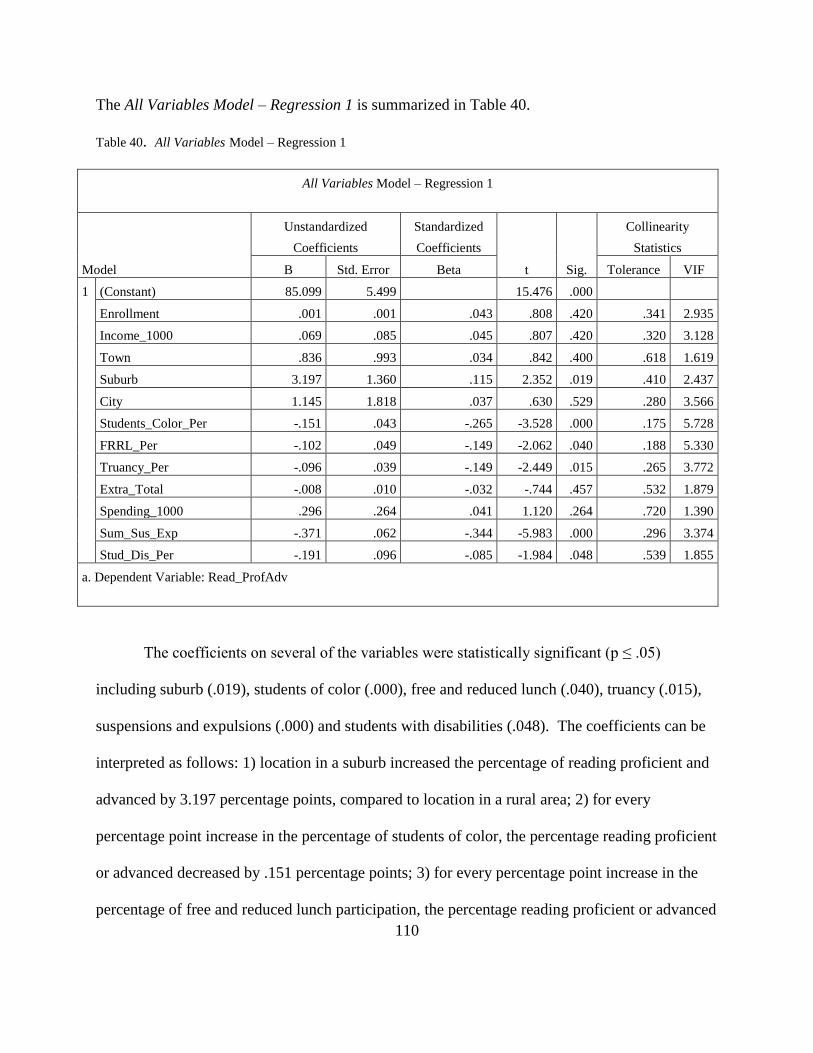
110

The All Variables Model – Regression 1 is summarized in Table 40.

Table 40. All Variables Model – Regression 1

All Variables Model – Regression 1

Model

Unstandardized

Coefficients

Standardized

Coefficients

t Sig.

Collinearity

Statistics

B Std. Error Beta Tolerance VIF

1 (Constant) 85.099 5.499 15.476 .000

Enrollment .001 .001 .043 .808 .420 .341 2.935

Income_1000 .069 .085 .045 .807 .420 .320 3.128

Town .836 .993 .034 .842 .400 .618 1.619

Suburb 3.197 1.360 .115 2.352 .019 .410 2.437

City 1.145 1.818 .037 .630 .529 .280 3.566

Students_Color_Per -.151 .043 -.265 -3.528 .000 .175 5.728

FRRL_Per -.102 .049 -.149 -2.062 .040 .188 5.330

Truancy_Per -.096 .039 -.149 -2.449 .015 .265 3.772

Extra_Total -.008 .010 -.032 -.744 .457 .532 1.879

Spending_1000 .296 .264 .041 1.120 .264 .720 1.390

Sum_Sus_Exp -.371 .062 -.344 -5.983 .000 .296 3.374

Stud_Dis_Per -.191 .096 -.085 -1.984 .048 .539 1.855

a. Dependent Variable: Read_ProfAdv

The coefficients on several of the variables were statistically significant (p ≤ .05)

including suburb (.019), students of color (.000), free and reduced lunch (.040), truancy (.015),

suspensions and expulsions (.000) and students with disabilities (.048). The coefficients can be

interpreted as follows: 1) location in a suburb increased the percentage of reading proficient and

advanced by 3.197 percentage points, compared to location in a rural area; 2) for every

percentage point increase in the percentage of students of color, the percentage reading proficient

or advanced decreased by .151 percentage points; 3) for every percentage point increase in the

percentage of free and reduced lunch participation, the percentage reading proficient or advanced

111

decreased .102 percentage points; 4) for every percentage point increase in the percentage of

students who were truant, the percentage reading proficient or advanced decreased .096

percentage points; 5) for every percentage point increase in the percentage of suspensions and

expulsions, the percentage reading proficient or advanced decreased .371 percentage points and

6) for every percentage point increase in the students with disabilities percentage, the percentage

of reading proficient or advanced decreased .191 percentage points. The signs on each of these

variables were the same as those reported in the research literature that used individual data to

analyze influences on reading achievement.

Although the results were clear and consistent with findings in other research, two types

of problems may have influenced the results, problems that could affect the interpretation and

policy implications.

First, the model demonstrated high variance inflation factors (VIF) and low tolerance

(one is the reciprocal of the other). A high VIF suggests that there are high correlations among

the variables that can create multicollinearity problems in the regression. The threshold for a

“high” VIF cannot be determined statistically but is a matter of judgment of the researcher.

Ideally, all VIF are less than 2, but some researchers choose thresholds of 3, 4 or even 6 in

judging the likelihood of multicollinearity in the model. In this study, a VIF of 3 was used in

identifying likely multicollinearity problems although, as will be discussed below, it was not

always possible to modify the model to produce VIF of 3 or less for all variables.

In Regression 1, the All Variables model, six variables had high VIF values that signaled

likely multicollinearity problems: average income by school district (3.128), city (3.566),

students of color (5.728), free and reduced lunch (5.330), truancy (3.772) and suspension and

112

expulsions (3.374). In the presence of multicollinearity, coefficient estimates are not biased, but

the standard errors will be inflated, thus leading to lower t-values, higher significance numbers

and less likely rejection of the null hypothesis that the coefficient is equal to zero. In addition,

the coefficient estimates may not be stable across different samples. Thus, these six variables

with high VIF may have created problems in interpretation of the results, so further analysis was

required to isolate this problem. The results of the analysis of multicollinearity will be discussed

in a separate section after the presentation section on the All Schools model, Regression 2.

Second, it is possible that outliers, high schools with extreme values for one or more of

the independent variables, exerted an extraordinary influence on the coefficient estimate. This is

a potential problem in any regression analysis, so an analysis of the possible effect of outliers

was carried out using the All Variables model. The analysis is presented below.

The first step in the outlier analysis was to create scatter plots to examine the distribution

of each variable and identify possible outliers. Appendix C includes a scatter plot for all

independent variables except geographic location variables that were straightforward by

definition. The distributions for five variables had outliers, a very small group of observations

well outside the distributional pattern of all the other observations. The variables with clearly

identifiable outlier clusters were the following: free and reduced lunch, students of color,

truancy, suspensions and expulsions and students with disabilities. Free and reduced lunch had

six city high schools with percentages greater than 77%; students of color had 10 high schools

(nine city and one rural) with percentages greater than 85%; nine high schools (eight city and one

rural) had percentages greater than 70% for truancy; suspensions and expulsions percentages

which were greater than 40% were in eight city high schools; and one city high school had a

113

students with disabilities percentage greater than 60%. Of those five variables with clear outlier

clusters, the same six city high schools were included in the outlier group for four of the five

variables, including free and reduced lunch, students of color, truancy and suspensions and

expulsions. Another city high school was an outlier for the variables students of color, truancy

and students with disabilities while yet another city high school was an outlier for the variables

students of color, truancy and suspensions and expulsions. Four high schools were in the outlier

group for one variable only: 1) one city high school for suspensions and expulsions, 2) one city

high school for students of color, 3) one rural high school for students of color and 4) one rural

high school for truancy. A new regression was calculated excluding the high schools that had an

outlier value for one or more of the variables; that is, they had free and reduced lunch <77%, or

students of color <85%, or truancy <70%, or suspensions and expulsions <40% or students with

disabilities <60%. The regression results showed coefficients that were very close to the values

estimated with the full sample of high schools in the All Variables model (see Table 40).

Removing the outlier cases produced results consistent with the All Variables regression.

Therefore, the outliers did not substantially influence the coefficient estimates.

All Schools Model

A second regression model was estimated, termed the All Schools model, with reading as

the dependent variable. Two of the ten independent variables could not be used in this model,

free and reduced lunch percentage and the students with disabilities percentage, because data for

these variables were not available for 104 high schools for grades 9-12 and WKCE scores were

not available for five schools (of which two were overlapping with the lack of information for

free and reduced lunch percentages and students with disabilities percentages). By removing the

114

variables free and reduced lunch and students with disabilities, a total of 412 schools were

included in the second regression model.

The second regression produced an r2 = .600, meaning that 60% of the variation in

reading proficient or advanced was explained by the eight remaining independent variables. The

model was also highly significant (.000).

The All Schools Model – Reading regression is summarized in Table 41.

Table 41. All Schools Model – Reading

All Schools Model - Readinga

Model

Unstandardized

Coefficients

Standardized

Coefficients

t Sig.

Collinearity

Statistics


1 (Constant) 72.637 4.501 16.139 .000

Enrollment .002 .001 .086 1.599 .111 .343 2.920

Income_1000 .250 .064 .163 3.912 .000 .575 1.740

Town .824 1.054 .031 .782 .434 .654 1.528

Suburb 3.352 1.477 .110 2.270 .024 .427 2.344

City -.577 1.975 -.017 -.292 .770 .305 3.277

Students_Color_Per -.145 .040 -.243 -3.657 .000 .226 4.431

Truancy_Per -.135 .039 -.193 -3.467 .001 .322 3.108

Extra_Total -.005 .011 -.020 -.474 .636 .561 1.781

Spending_1000 .327 .255 .048 1.282 .201 .704 1.421

Sum_Sus_Exp -.385 .058 -.350 -6.579 .000 .354 2.827


Again, the coefficients on several of the variables were statistically significant (p ≤ .05),

including average income by school district (.000), suburb (.024), students of color (.000),

truancy (.001) and suspensions and expulsions (.000). The coefficients can be interpreted as

follows: 1) for every $1,000 dollar increase in average income by school district, the percentage

115

reading proficient or advanced increased .250 percentage points; 2) location in a suburb

increased the percentage reading proficient or advanced by 3.353 percentage points, compared to

location in a rural area; 3) for every percentage point increase in the percentage of students of

color, the percentage reading proficient or advanced decreased .145 percentage points; 4) for

every percentage point increase in the percentage of students who were truant, the percentage

reading proficient or advanced decreased .135 percentage points; 5) for every percentage point

increase in the percentage of students suspended or expelled, the percentage reading proficient or

advanced decreased .385 percentage points. The signs on each of these variables are the same as

those reported in the research literature that used individual data to analyze influences on reading

achievement.

Although the All Schools model demonstrated a substantial reduction in multicollinearity

compared to the All Variables model, high VIF were associated with three variables: city

(3.277), students of color (4.431) and truancy (3.108).

As in the All Variables model, a separate regression was calculated with the removal of

high schools included in any of the outlier clusters. Thus, a school was removed from the

analysis if it had the following: free and reduced lunch <77%, or students of color <85%, or

truancy <70%, or suspensions and expulsions <40% or students with disabilities <60%. The

regression results were consistent with the All Schools regression (see Table 41). Thus, schools

with extreme values on the independent variables were not a problem and did not influence the

results of the regression for the All Schools model.

In conclusion, the results from the All Variables Model - Regression 1 and All Schools

Model - Regression 2 were fundamentally identical. Both had essentially the same statistically

116

significant coefficients. The All Variables Model statistically significant coefficients included

suburb, students of color, free and reduced lunch, truancy, suspensions and expulsions and

students with disabilities while the All Schools Model statistically significant coefficients

included average income, suburb, students of color, truancy and suspensions and expulsions.

Both regressions included the statistically significant coefficients of suburb, students of color,

truancy and suspensions and expulsions. Suburb had a positive relationship with reading

proficient or advanced percentage in both regressions while students of color, truancy and

suspensions and expulsions had a negative relationship with the percentage reading at proficient

or advanced in both regression equations. Both regressions also produced the same conclusions

about geographic location. Location in a town or a city did not produce reading results different

from location in a rural area – the coefficients on town and city were not statistically

significantly different from zero, the value of the excluded rural location variable. However, the

coefficient on the variable suburb was positive and statistically significant, meaning that location

in a suburb was associated with a higher percentage of students reading at the proficient or

advanced levels. Also, all of the coefficients on the variables were exactly as predicted by the

theory and consistent with empirical results using individuals rather than schools as the unit of

analysis. Thus, it was very unlikely that the ecological fallacy was present in these regression

results. Overall, the regression analysis was reassuring because the results for the geographic

location variable were the same no matter which model was used or whether outliers were

included or excluded.

Analysis of Multicollinearity

The VIF data for both the All Variables and the All Schools models showed likely

117

problems with multicollinearity in the regressions. The analysis of multicollinearity proceeded

in two different ways: 1) omitting highly correlated variables and 2) factor analysis to reduce a

cluster of highly correlated variables into a single measure. The All Variables model was used

for the multicollinearity analysis because it showed the highest levels of multicollinearity and

because all of the variables with high VIF values in the All Schools model also had high VIF

values in the All Variables model. Thus, eliminating the multicollinearity problem in the All

Variables model would very likely eliminate it in the All Schools model as well.

The All Variables model showed high multicollinearity in the following six variables

listed from highest to lowest VIF values: 1) students of color (5.728), 2) free and reduced lunch

(5.330), 3) truancy (3.772), 4) city (3.566), 5) suspensions and expulsions (3.374) and 6) average

income by school district (3.128). The variable for students of color was retained in the

regression since a large amount of research and discussion is focused on the academic

achievement of students of color. In addition, the geographic variable City was retained in the

regression because the effect of geographic location on achievement was the core question in this

study, and City could not be eliminated without affecting the coefficients on the other geographic

location variables. Therefore, the regression equation was estimated three additional times

removing the following variables: 1) free and reduced lunch, 2) free and reduced lunch and

truancy and 3) free and reduced lunch, truancy and suspensions and expulsions. The purpose was

to examine the change in the VIF multicollinearity diagnostic and, in particular, to determine

whether VIF might be reduced to ≤ 3.00 for all variables. After the removal of free and reduced

lunch, overall multicollinearity decreased, but four variables still had high VIF values, including

city (3.561), students of color (5.339), truancy (3.768) and suspensions and expulsions (3.168).

118

After the removal of free and reduced lunch and truancy, the VIF values decreased again, but

two variables had high VIF including city (3.560) and students of color (4.843). Lastly, after the

removal of free and reduced lunch, truancy and suspensions and expulsions, two variables had

collinearity including city (3.517) and students of color (3.033). Although the multicollinearity

improved after removing one, two and then three variables, the procedure was not fully effective

in eliminating all of the multicollinearity (VIF ≤ 3.00) for all variables, and removing three

variables for the analysis was not consistent with the underlying theoretical model in the study.

Since the removal of variables was not fully effective, factor analysis was used to collapse

several highly correlated variables into a single index.

Factor Analysis

Factor analysis was used to create one or more variables that were based on, and derived

from, the common variation of the highly correlated cluster of variables in the model. Factor

analysis is often used to extract a common “factor” or unmeasured but important concept (or

concepts) from a set of variables. For example, factor analysis might be used to construct a

variable measuring a “factor” called “health status” of a population based on indicators, such as

infant mortality, life expectancy, incidence of preventable communicable diseases and other

indicators that have high levels of correlation among them. Two methods were used in this study

to construct variables to capture the common variation of the variables with high VIF values in

the regression analysis. First, a simple conceptual model was used to sort the highly correlated

variables into two groups, and a single factor was extracted for each group. Second, the five

highly correlated variables were included in a single factor analysis, in effect allowing the factor

analysis algorithm to empirically define the groups.

119

First, a POVERTY factor was created using average income by school district, students

of color and free and reduced lunch participation, all indicators associated with family socio-

economic status. The variables truancy and suspensions and expulsions were used in a second

factor analysis, and the factor capturing the common variation was termed OUT_OF_SCHOOL.

Using the results of the factor analysis, factor scores were created for each high school for each

of the factor analysis factors. These factor scores were then used as independent variables in the

regression analysis in place of the highly correlated variables used to create the factors. In the

regression including the factor analysis variables POVERTY and OUT_OF_SCHOOL, the

results are presented in Table 42.

Table 42. Factor Analysis 1 – POVERTY & OUT_OF_SCHOOL

Factor Analysis 1 – POVERTY & OUT_OF_SCHOOL

Model

Unstandardized

Coefficients

Standardized

Coefficients

t Sig.

Collinearity

Statistics


1 (Constant) 80.269 3.944 20.353 .000

Enrollment .001 .001 .034 .624 .533 .343 2.912

Town .862 1.006 .035 .857 .392 .622 1.607

Suburb 2.315 1.324 .083 1.749 .081 .447 2.238

City -.394 1.734 -.013 -.227 .820 .318 3.144

Extra_Total -.003 .010 -.012 -.282 .778 .554 1.805

Spending_1000 .139 .261 .019 .532 .595 .759 1.317

Stud_Dis_Per -.147 .093 -.065 -1.580 .115 .591 1.691

OUT_OF_

SCHOOL

-5.719 .516 -.565 -11.076 .000 .389 2.571

POVERTY -2.947 .618 -.278 -4.768 .000 .298 3.352


120

The statistically significant coefficients (p ≤ .05) were the two new factors, OUT_OF_SCHOOL

(.000) and POVERTY (.000). However, the coefficient on suburb was not statistically

significantly different from zero (.081) in this model. Unfortunately, evidence of

multicollinearity still existed in the form of high VIF values for two variables including city

(3.144) and poverty (3.352).

The second factor analysis approach was to allow the software algorithms to determine

empirical associations and extract factors from the variables using students of color, average

income by school district, free and reduced lunch, truancy and suspensions and expulsions. The

results showed that the variables students of color, free and reduced lunch, truancy and

suspensions and expulsions loaded heavily and positively on the first extracted factor

(FACTOR_1) while average income by school district loaded heavily and positively, and free

and reduced lunch loaded somewhat heavily and negatively on the second factor (FACTOR_2)

(See Appendix D). These two factor loadings were then used to calculate factor scores for each

high school, and the resulting variables were used within a regression. The results are below in

Table 43.

121

Table 43. Factor Analysis 2 – FACTOR_1 & FACTOR_2

Factor Analysis 2 – FACTOR_1 & FACTOR_2a

Model

Unstandardized

Coefficients

Standardized

Coefficients

t Sig.

Collinearity Statistics


1 (Constant) 78.848 3.852 20.468 .000

Enrollment .001 .001 .045 .843 .400 .342 2.928

Town .956 .995 .038 .961 .337 .622 1.608

Suburb 3.241 1.347 .117 2.406 .017 .422 2.368

City 1.039 1.732 .034 .600 .549 .312 3.206

Extra_Total -.008 .010 -.032 -.749 .454 .549 1.822

Spending_1000 .260 .253 .036 1.027 .305 .790 1.266

Stud_Dis_Per -.146 .092 -.065 -1.582 .115 .592 1.688

FACTOR_1 -7.426 .521 -.733 -14.246 .000 .375 2.670

FACTOR_2 1.769 .506 .166 3.495 .001 .438 2.283


The statistically significant coefficients (p ≤ .05) were suburb (.017), FACTOR_1 (.000) and

FACTOR_2 (.001). Evidence of multicollinearity existed in the form of high VIF values for one

variable, City (3.206). The coefficient on the suburb variable was again statistically significant

and was at approximately the same magnitude as the regressions including all five of the

variables rather than the factors. Unfortunately, the VIF values still indicate potential problems

with multicollinearity. In the end, the use of factor analysis reduced but did not eliminate the

problems with multicollinearity in the model

Base Model Selection

The regression results with the percent proficient or advanced in reading as the dependent

variable were used to analyze the differences between the All Variables and the All Schools

models, the effect of removing high schools with extreme values on some of the independent

122

variables, and the differences that might result from omitting variables or using factor analysis to

overcome multicollinearity problems. The coefficient estimates and significance levels for the

variables were remarkably stable across all of these analyses. This suggested that a single base

model can be used in the analysis without loss of explanatory power and with some assurance

that the conclusions would be stable across many types of variations in the observations and

variables included in the model.

Since the essential research question was to study how rural high schools’ academic

achievement compares to that in other town, suburb and city high schools, it was logical to

include as many schools in the data set as possible. Although the All Schools Model was not

perfect, the All Variables Model removed 104 schools from the data set due to lack numbers for

free and reduced lunch and students with disabilities, leaving only 310 high schools for data

analysis. Using the All Schools Model would allow for 412 schools data to be analyzed.

The major drawback of the All Schools Model was that the variables, free and reduced

lunch and students with disabilities, could not be used in the analysis. But average income by

school district was highly correlated with free and reduced lunch, accounting for 55% of the

variation using the bivariate correlation coefficient and about the same percentage using the

partial correlation coefficient in the regressions. Therefore, average income by school district

was a reasonable proxy for the poverty concept that underlies both the income and free and

reduced lunch variables. In addition, although the students with disabilities variable could not be

replaced or accounted for with a proxy, the effect of students with disabilities on academic

achievement is a well known, especially the effects of cognitive disability on test scores.

Second, this variable was not highly correlated with the geographic location variables so

123

excluding it would not likely result in a substantial bias to the coefficient estimates or

significance levels. Therefore, although it would have been desirable to include this variable in

the model, it was not necessary, and excluding it in order to include more schools in the analysis

was a reasonable concession.

The base model could potentially have included the variables created from the factor

scores in the factor analysis. However, including these variables did not solve the

multicollinearity issues and would have omitted variables with more clear interpretations. For

example, factor analysis was used to create a variable to capture the common variation among

students of color, truancy and suspensions and expulsions. Including this factor variable in the

regression produced similar coefficient and VIF results as using the variables themselves. Yet in

the regression with the three variables included, the coefficients on all three variables were all

highly significant despite inflation in the coefficient of standard error caused by

multicollinearity. Thus, the only remaining variable with high VIF values was City, and this

variable could not be excluded or submerged in a factor because geographic location was central

to the research question in the study. Therefore, using factor analysis would not improve the

base model beyond the use of the underlying variables themselves, and thus the factor variables

were not included in the base model.

In summary, the All Schools Model was used as the base model. The All Schools Model

has shown stable results across several specifications of the model. It was very clear that this is a

highly stable model.

READING

The All Schools Model – Reading regression was discussed in detail above (see Table

124

41), and the coefficients and significance levels will not be repeated here. The regression

included 412 high schools in the data set with r2 = .600, meaning that 60% of the variation in

reading proficient or advanced was explained by the eight remaining independent variables, and

the model was highly significant (.000).

LANGUAGE ARTS

The All Schools Model – Language Arts regression summarized in Table 44 included 412

high schools in the data set with r2 = .537, meaning that 53.7% of the variation among high

schools in the percentage of students at the proficient or advanced in language arts was explained

by variation in the eight independent variables. The model was also highly significant (.000).

Table 44. All Schools Model – Language Arts

All Schools Model – Language Artsa

Model

Unstandardized

Coefficients

Standardized

Coefficients

t Sig.

Collinearity

Statistics


1 (Constant) 54.758 5.328 10.277 .000

Enrollment .001 .001 .030 .524 .601 .343 2.920

Income_1000 .450 .076 .267 5.951 .000 .575 1.740

Town 1.905 1.247 .064 1.528 .127 .654 1.528

Suburb 5.019 1.748 .149 2.871 .004 .427 2.344

City 1.083 2.338 .028 .463 .644 .305 3.277

Students_Color_

Per

-.122 .047 -.185 -2.585 .010 .226 4.431

Truancy_Per -.113 .046 -.147 -2.448 .015 .322 3.108

Extra_Total -.010 .012 -.035 -.765 .445 .561 1.781

Spending_1000 .639 .302 .086 2.116 .035 .704 1.421

Sum_Sus_Exp -.427 .069 -.352 -6.169 .000 .354 2.827

a. Dependent Variable: LA_ProfAdv

125

Results showed that the coefficients on several of the variables were statistically

significant (p ≤ .05) including the positive correlations on average income by school district

(.000), spending per pupil (.035) and suburb (.004), and the negative coefficients on students of

color (.010), truancy (.015) and suspensions and expulsions (.000). The coefficients on the

variables enrollment, town, city and extra/co-curricular participation index were not statistically

significant at the .05 level.

The statistically significant factors can be interpreted as follows: 1) for every $1,000

dollar increase in average income per school district, the percentage of proficient or advanced in

language arts increased .450 percentage points; 2) a high school located in the suburb scored

5.019 percentage points higher than a high school located in a rural area; 3) for every percentage

point increase in the percentage of students of color, the percentage of students proficient or

advanced in language arts decreased by .122 percentage points; 4) for every percentage point

increase in truancy percentage, the percentage of students proficient or advanced in language arts

decreased by .113 percentage point; 5) for each additional $1,000/pupil in school district

spending, the percentage of students proficient or advanced in language arts increased .639

percentage points and 6) for every percentage point increase in the percentage of suspensions and

expulsions, the percentage of students proficient or advanced in language arts decreased .427

percentage points.

MATHEMATICS

The All Schools Model – Mathematics regression summarized in Table 45 included 412

high schools in the data set with r2 = .575, meaning that 57.5% of the variation among high

126

schools in the percentage of students at the proficient or advanced in mathematics was explained

by the variation in eight independent variables. The model was also highly significant (.000).

Table 45. All Schools Model – Mathematics

All Schools Model - Mathematicsa

Model

Unstandardized

Coefficients

Standardized

Coefficients

t Sig.

Collinearity

Statistics


1 (Constant) 59.646 5.404 11.037 .000

Enrollment .002 .001 .102 1.826 .069 .343 2.920

Income_1000 .419 .077 .234 5.457 .000 .575 1.740

Town -.711 1.265 -.023 -.562 .574 .654 1.528

Suburb 2.170 1.773 .061 1.224 .222 .427 2.344

City 1.108 2.371 .028 .467 .641 .305 3.277

Students_Color_

Per

-.192 .048 -.277 -4.036 .000 .226 4.431

Truancy_Per -.107 .047 -.131 -2.277 .023 .322 3.108

Extra_Total .003 .013 .009 .204 .839 .561 1.781

Spending_1000 .449 .306 .057 1.466 .143 .704 1.421

Sum_Sus_Exp -.453 .070 -.354 -6.459 .000 .354 2.827

a. Dependent Variable: Math_ProfAdv

Results showed that the coefficients on four variables were statistically significant at p ≤

.05 including the positive coefficients on average income by school district (.000) and the

negative coefficients on students of color (.000), truancy (.023) and suspensions and expulsions

(.000). The coefficients on the variables enrollment, town, suburb, city, extra/co-curricular

participation index and spending per pupil were not statistically significant at the .05 level.

The statistically significant coefficients can be interpreted as follows: 1) for each

additional $1,000/pupil in school district spending, the percentage of students proficient or

127

advanced in mathematics increased .419 percentage points; 2) for every percentage point

increase in the percentage of students of color, the percentage of proficient or advanced in

mathematics decreased .192 percentage points; 3) for every percentage point increase in the

percentage of truancy, the percentage of proficient or advanced decreased .107 percentage points

and 4) for every percentage point increase in suspensions and expulsions percentage, the

percentage of proficient or advanced in mathematics decreased .453 percentage points.

SCIENCE

The All Schools Model – Science regression summarized in Table 46 included 412 high

schools in the data set with r2 = .606, meaning that 60.6% of the variation among high schools in

the percentage of students at the proficient or advanced in science was explained by the variation

in the eight independent variables. The model was highly significant (.000).

128

Table 46. All Schools Model – Science

All Schools Model - Sciencea

Model

Unstandardized

Coefficients

Standardized

Coefficients

t Sig.

Collinearity

Statistics


1 (Constant) 61.485 5.098 12.060 .000

Enrollment .001 .001 .053 .982 .327 .343 2.920

Income_1000 .392 .072 .224 5.422 .000 .575 1.740

Town .556 1.193 .018 .466 .642 .654 1.528

Suburb 2.028 1.673 .058 1.212 .226 .427 2.344

City .025 2.237 .001 .011 .991 .305 3.277

Students_Color_

Per

-.249 .045 -.366 -5.545 .000 .226 4.431

Truancy_Per -.061 .044 -.077 -1.392 .165 .322 3.108

Extra_Total -.001 .012 -.005 -.109 .913 .561 1.781

Spending_1000 .668 .289 .086 2.313 .021 .704 1.421

Sum_Sus_Exp -.422 .066 -.336 -6.377 .000 .354 2.827

a. Dependent Variable: Science_ProfAdv

Results showed that the coefficients on four variables were statistically significant at p ≤

.05 including the positive coefficients on average income by school district (.000) and spending

per pupil (.021) and the negative coefficients on students of color (.000) and suspensions and

expulsions (.000). The coefficients on the variables enrollment, town, suburb, city, truancy and

extra/co-curricular participation index were not statistically significant at the .05 level.

The statistically significant coefficients can be interpreted as follows: 1) for every $1,000

dollar increase in average income by school district, the percentage of students proficient or

advanced in science increased .392 percentage points; 2) for every percentage point increase in

the percentage of students of color, the percentage of proficient or advanced in science decreased

129

.249 percentage points; 3) for each additional $1,000/pupil in school district spending, the

percentage of proficient and advanced in science increased .668 percentage points and 4) for

every percentage point increase in the percentage of suspensions and expulsions, the percentage

of proficient or advanced in science decreased .422 percentage points.

SOCIAL STUDIES

The All Schools Model – Social Studies regression summarized in Table 47 included 412

high schools in the data set with r2 = .590, meaning that 59% of the variation among high

schools in the percentage of students at the proficient or advanced in social studies was explained

by variation in the eight independent variables. The model was also highly significant (.000).

Table 47. All Schools Model – Social Studies

All Schools Model – Social Studiesa

Model

Unstandardized

Coefficients

Standardized

Coefficients

t Sig.

Collinearity

Statistics


1 (Constant) 71.835 4.801 14.964 .000

Enrollment .001 .001 .063 1.148 .252 .343 2.920

Income_1000 .289 .068 .179 4.242 .000 .575 1.740

Town .997 1.124 .035 .887 .375 .654 1.528

Suburb 3.780 1.575 .117 2.399 .017 .427 2.344

City 1.636 2.106 .045 .777 .438 .305 3.277

Students_Color_

Per

-.145 .042 -.230 -3.416 .001 .226 4.431

Truancy_Per -.158 .042 -.214 -3.802 .000 .322 3.108

Extra_Total -.012 .011 -.047 -1.098 .273 .561 1.781

Spending_1000 .290 .272 .041 1.067 .286 .704 1.421

Sum_Sus_Exp -.427 .062 -.368 -6.844 .000 .354 2.827

a. Dependent Variable: SS_ProfAdv

130

Results showed that the coefficients on five variables were statistically significant at p ≤

.05 including the positive coefficients on average income by school district (.000) and suburb

(.017) and the negative coefficients on students of color (.001), truancy (.000) and suspensions

and expulsions (.000). The coefficients on the variables enrollment, town, city and extra/co-

curricular participation index were not statistically significant at the .05 level.

The statistically significant coefficients can be interpreted as follows: 1) for every $1,000

dollar increase in average income by school district, the percentage of students proficient or

advanced in social studies increased .289 percentage points; 2) a high school located in the

suburb scored 3.780 percentage points higher than a high school located in a rural area; 3) for

every percentage point increase in the percentage of students of color, the percentage of

proficient or advanced in social studies decreased .145 percentage points; 4) for every percentage

point increase in the percentage of truancy, the percentage of proficient or advanced in social

studies decreased .158 percentage points and 5) for every percentage point increase in the

percentage of suspensions and expulsions, the percentage of proficient or advanced in science

decreased .427 percentage points.

RURAL LOCATION AND ACADEMIC ACHIEVEMENT

Table 48 provides a summary of the results for all the regressions. The number in each

cell is the standardized coefficient (beta); the number of standard deviation changes in the

advanced or proficient dependent variable from a one standard deviation change in the

independent variable. The relative magnitude of the effects of the independent variables can be

assessed by comparing the absolute value of the standardized coefficients. Coefficients

131

significant at the .05 level are noted with a single asterisk next to the value in the cell, and the

significance at the .01 level or better is noted with two asterisks.

Table 48. Base Model Regression Summary

Reading Language Arts Mathematics Science Social Studies

Enrollment .086 .030 .102 .053 .063

Income_1000 .163** .267** .234** .224** .179**

Town .031 .064 -.023 .018 .035

Suburb .110* .149** .061 .058 .117*

City -.017 .028 .028 .001 .045

Students_Color_Per -.243** -.185** -.277** -.366** -.230**

Truancy_Per -.193** -.147* -.131* -.077 -.214**

Extra_Total -.020 -.035 .009 -.005 -.047

Spending_1000 .048 .086* .057 .086* .041

Sum_Sus_Exp -.350** -.352** -.354** -.336** -.368**

r2

.600 .537 .575 .606 .590

Model Significance .000** .000** .000** .000** .000**

** Correlation is significant at the 0.01 level.

*Correlation is significant at the 0.05 level.

Enrollment was not significant in any of the five subject areas regressions. Although

previous research has concluded that the size of a school is important, when controlling for other

variables as within this study, the coefficients on enrollment were not significant.

Average income by school district had a significant coefficient at the p ≤ .01 levels for all

five subject areas. The null hypothesis is that the coefficient on average income by school

district is zero, H0: Income_1000 = 0. Based on the significance levels, the null hypothesis that

the coefficient is equal to zero was rejected in every case. The alternative hypothesis H1 =

132

Income_1000 ≠ 0 was accepted because the results were highly significant and consistent. Thus,

as income increased, the percentage of students proficient or advanced also increased. The effect

of average income was positive and statistically significant for reading, language arts,

mathematics, science and social studies. Overall, average income by school district has a

positive relationship to academic achievement. Furthermore, comparing the magnitude of the

standardized coefficients, the impact of average family income on the percent at proficient or

advanced levels was always greater than the impact of the geographic variable and spending per

pupil. It was also always smaller than the impact of the suspension/expulsion variable and

usually smaller than the impact of increases in the percentage of students of color. Average

family income was usually greater than the impact of increases in the percentage of truancy.

The effect of geographical locations of rural, town, suburb and city on academic

achievement was the central interest in this study. In the reading regression, the coefficients on

town and city were not statistically significantly different from zero; however, the coefficient on

suburb was positive and statistically significant at p ≤ .05 levels but with low impact compared

to other independent variables with significant coefficients. In language arts, town and city were

not statistically significant. But suburb was positive and statistically significant at the p ≤ .01

levels but again with low impact compared to other independent variables with significant

coefficients. In the regressions with mathematics and science as the dependent variables, neither

town, suburb nor city had statistically significant coefficients. In social studies, town and city

were not statistically significant at p ≤ .05 levels; whereas, suburb was statistically significant but

with low impact compared to other independent variables with significant coefficients.

Compared to rural, location in a suburb was associated with higher test scores in reading,

133

language arts and social studies but not in mathematics or science. Compared to rural, location

in a town or city had no effect on test scores in any subject area. Overall, geographic location

was not a strong predictor of academic achievement. It is clear that location in a rural school is

not associated with lower test scores, relative to location in town or city. Location in a suburb is

associated with higher test scores, compared to rural, in reading, language arts and social studies,

but not in math or science. But even when the coefficient on the suburb variable was significant,

the magnitude of the effect was low compared to the variables representing average family

income, the percentage students of color, and the percentage suspensions/expulsions.

Students of color had negative and significant coefficients at the p ≤ .01 levels for all

five-subject areas. The null hypothesis was that the coefficient for students of color was equal to

zero, i.e. H0: Students_Color_Per = 0. Based on the significance levels, the null hypothesis was

rejected for every subject area. The alternative hypothesis H1 = Students_Color_Per ≠ 0 was

accepted because the significant levels were strong; the coefficient was negative in every case,

and the magnitude of the effect was large compared to other coefficients. Thus, increases in the

percentage of students of color was associated with decrease in the percentage at the proficient or

advanced levels in reading, language arts, mathematics, science and social studies. In summary,

the students of color variable had a negative relationship to academic achievement, and its

impact was fairly large compared to the impact of other variables.

Truancy had a negative and significant coefficient at the p ≤ .01 levels in reading and

social studies and at the p ≤ .05 levels in language arts and mathematics. The coefficient on

truancy was not statistically significant in the regressions with science as the dependent variable.

134

The null hypothesis was that the coefficient for truancy was equal to zero, i.e. H0: Truancy_Per =

0. Based on the significance levels in reading, language arts, mathematics and social studies, the

null hypothesis was rejected in four subject areas. The alternative hypothesis H1 = Truancy_Per

≠ 0 was accepted because the significance level was strong, and the coefficient was negative in

every case. But the magnitude of the effect was relatively small compared to other coefficients.

However, in science the null hypothesis H0: Truancy_Per = 0 was not rejected, and judgment

was withheld. Thus, increases in truancy were associated with decreases in the percentage of

proficient or advanced levels in reading, language arts, mathematics and social studies.

Therefore, the truancy variable had a negative relationship to academic achievement but only

affects four of the five subject areas. Furthermore, comparing the magnitude of the standardized

coefficients, the impact of truancy on the percent at proficient or advanced levels was always

greater than spending per pupil and always smaller than the impact of the students of color and

suspensions and expulsions variables.

The coefficient on the extra/co-curricular participation index was not statistically

significant in any regression within this study. Although the coefficients were never significant,

there is literature that exists stating participation in extra/co-curricular activities is positively

associated with student achievement. However, when controlling for the effects of several other

variables as within this study, the coefficient on the extra/co-curricular participation index was

not statistically significant in any of the five subject area regressions.

Spending per pupil had a positive and significant coefficient at the p ≤ .05 levels in

language arts and science. Spending per pupil was not statistically significant in reading,

135

mathematics or social studies. The null hypothesis was that the coefficient for spending per

pupil was equal to zero, i.e. H0: Spending_1000 = 0. Based on the significance levels in

language arts and science, the null hypothesis was rejected in these two subject areas. The

alternative hypothesis H1 = Spending_1000 ≠ 0 was accepted because the significance levels

were strong and the coefficient was positive in both cases. However, the magnitude of the effect

was low compared to the other variables representing average income by school district, the

percentage of students of color, truancy and suspensions and expulsions. In the regressions for

reading, mathematics and social studies, the null hypothesis H0: Spending_1000 = 0 was

accepted. Thus, for each additional $1,000/pupil in school district spending, the percentage at

the proficient or advanced levels increased in language arts and science. In summary, spending

per pupil has a positive relationship with academic achievement but is specific to language arts

and science. Furthermore, comparing the magnitude of the standardized coefficients, the impact

of spending per pupil on the percent at proficient or advanced levels was always smaller than the

impact of the average income by school district, suburb, students of color, truancy, spending per

pupil and suspensions and expulsions variables.

Lastly, suspensions and expulsions had a negative and significant coefficient at the p ≤

.01 levels for all five-subject areas. The null hypothesis was that the coefficient for suspensions

and expulsions was equal to zero, i.e. H0: Sum_Sus_Exp = 0. Based on the significance levels,

the null hypothesis was rejected for every subject area. The alternative hypothesis H1 =

Sum_Sus_Exp ≠ 0 was accepted because the significance levels were strong; the coefficient was

negative in every case, and the magnitude of the effect was the largest compared to all other

136

coefficients. Thus, increases in suspensions and expulsions were associated with decreases in the

percentage at the proficient or advanced levels in reading, language arts, mathematics, science

and social studies. Therefore, suspensions and expulsions had a negative and statistically

significant relationship with academic achievement in all five subject areas. Furthermore,

comparing the magnitude of the standardized coefficients, the impact of suspensions and

expulsions on the percent at proficient or advanced levels was always greater than the impact of

the average income by school district, suburb, students of color, truancy and spending per pupil

variables.

In summary, the variables of students of color and suspensions and expulsions had large

and very statistically significant impact on the percentage of students at the proficient or

advanced levels in reading, language arts, mathematics, science and social studies. Truancy also

had an impact on four subject areas. High and positive correlations of the variables percentage

of students of color, percentages of suspensions and expulsions and percentages of truancy

existed with the geographic location variable City. Average income by school district and

spending per pupil also illustrated a positive relationship to academic achievement. Lastly, the

effect of location in a suburb was positive and significant in three subject areas, but the impact

was small compared to other variables. Overall, geographic location itself was not a strong

predictor of academic achievement; however, the negative strength of the variables students of

color, disciplinary actions: suspensions and expulsions and truancy influenced city schools

substantially.

137

CHAPTER 5

CONCLUSIONS, RECOMMENDATIONS & SUMMARY

Introduction

A study analyzing the relationship between academic achievement and geographic

location had never been conducted in the state of Wisconsin. Since rural high schools (229)

make-up 54.9% of the high schools in Wisconsin, it is essential to understand their value and

importance. In addition, since school funding will be drastically cut in the next state biennial

budget, this study is timely and provides valuable information to educate policy makers and

educational leaders about the worth of rural schools.

This study analyzed the academic achievement of rural high schools compared to city,

suburb and town high schools. The research methodology for this study was a quantitative, non-

experimental, ex post facto design using mined data from several state and federal public

databases. The sample size included 412 public high schools in the state of Wisconsin but did

not include Wisconsin high schools that were parochial, alternative, charter, single purpose or

juvenile detention centers.

138

The purpose of this study was to distinguish how rural Wisconsin high students

performed on the tenth grade WKCE in the areas of Reading, Language Arts, Mathematics,

Science and Social Studies compared to Wisconsin city, suburb and town public high students.

This study included ten independent variables (i.e. geographic location, SES, students of color,

spending per pupil, high school enrollment, parent education level, truancy, disciplinary action:

suspensions and expulsions, students with disabilities and extra/co-curricular participation) and

five dependent variables (i.e. performance on WKCE tests in Reading, Language Arts,

Mathematics, Science and Social Studies). Regression analyses were used to analyze all five

areas of academic achievement while controlling for all ten dependent variables.

This study was important because it comes at a time of substantial budget cuts for

Wisconsin school districts. These cuts may force rural school districts to consider other

organizational arrangements or educational options in order to survive. These alternative

arrangements and options include referenda for operational expenses, cooperative agreements

with other school districts and school consolidation. Due to the decrease in state funding and

restrictive revenue controls, school districts in Wisconsin have difficult choices to make on

future staffing, curricula offerings and opportunities for its students.

In addition, a reduced state financial commitment to public schools may cause legislators

and other educational policy makers to discuss consolidation or other organizational

arrangements that threaten the existence of rural school districts. Since 229 high schools in the

state of Wisconsin are in rural locations, it was especially important at this time to discover how

rural high schools compared to its city, suburb and town peers. Similar studies had been

conducted in Arkansas, Kentucky, Montana, North Dakota, Ohio, Texas and West Virginia

139

comparing academic achievement and high school location, but never before in Wisconsin.

RESEARCH CONCLUSIONS

Regarding Geographical Location and Achievement

The purpose of this study was to distinguish how Wisconsin rural high students

performed on the tenth grade WKCE in the areas of Reading, Language Arts, Mathematics,

Science and Social Studies compared to Wisconsin city, suburb and town public high students.

The conclusions with respect to the effect of the geographical location of rural, town,

suburb and city on academic achievement were the central interest in this study. The conclusions

from the data analyses regarding academic performance and geographic location follow:

In the reading regression, the coefficients on town and city were not statistically

significantly different from zero; however, the coefficient on suburb was positive and

statistically significant at p ≤ .05 levels.

In language arts, the coefficients on town and city were not statistically significant. But

suburb was positive and statistically significant at the p ≤ .01 levels.

In the regressions with mathematics and science as the dependent variables, neither town,

suburb nor city had statistically significant coefficients.

In social studies, town and city were not statistically significant; whereas, suburb was

statistically significant at the p ≤ .05 levels.

From the data analysis, one can, therefore, conclude that compared to rural, location in a

suburb was associated with higher test scores in reading, language arts and social studies but not

in mathematics or science. Compared to rural, location in a town or city had no effect on test

scores in any subject area. Overall, geographic location was not a strong predictor of academic

140

achievement. It was clear that location in a rural school was not associated with lower test

scores, relative to location in town or city. Location in a suburb was associated with higher test

scores, compared to rural, in reading, language arts and social studies, but not in math or science.

But even when the coefficient on the suburb variable was significant, the magnitude of the effect

was low compared to the variables representing average family income, the percentage students

of color, and the percentage suspensions/expulsions.

Regarding the Dependent Variables and the Other Independent Variables

With respect to the five dependent variables, the following additional conclusions can be

made from the data analysis:

The coefficients on several of the independent variables with respect to reading were

statistically significant including average income by school district, suburb, students of

color, truancy and suspensions and expulsions. The relationships of each of these

variables were the same as those reported in the research literature that used individual

data to analyze influences on reading.

The coefficients on several of the independent variables with respect to language arts

were statistically significant including average income by school district, suburb, students

of color, truancy, spending per pupil and suspensions and expulsions. The relationships

among these signs on each of these variables were the same as those reported in the

research literature that used individual data to analyze influences on language arts

achievement.

The coefficients on several of the independent variables with respect to mathematics were

141

statistically significant including average income by school district, students of color,

truancy and suspensions and expulsions. The relationships among these variables

mirrored those reported in the research literature that used individual data to analyze

influences on mathematics achievement.

The coefficients on several of the independent variables with respect to science were

statistically significant including average income by school district, students of color,

spending per pupil and suspensions and expulsions. The relationships among these

variables were the same as those reported in the research literature that used individual

data to analyze influences on science achievement.

The coefficients on several of the independent variables with respect to social studies

were statistically significant including average income by school district, suburb, students

of color, truancy and suspensions and expulsions. The relationships of these variables

were the same as those reported in the research literature that used individual data to

analyze influences on social studies achievement.

Regarding the Independent Variables

Originally, ten independent variables were identified by the literature as having an impact

on student achievement. However, two of these variables, free and reduced lunch (the surrogate

for SES) and students with disabilities, were not included in the analysis because data were not

available on these two measures for 104 high schools in Wisconsin. Average income by school

district was available, however, and a reasonable proxy for the poverty concept that underlies

both the income and free and reduced lunch variables. In addition, although the students with

142

disabilities variable could not be replaced or accounted for with a proxy, the effect of students

with disabilities on academic achievement is well known, especially the effects of cognitive

disability on test scores. Thus, the researcher chose to use the All Schools model with the

population size of 412 schools and did not use the two previously identified independent

variables.

With respect to the eight remaining independent variables, the following conclusions (not

including those about rural location which were discussed previously) emerged from the data

analyses.

Students of color had negative and significant coefficients at the p ≤ .01 levels for all five

subject areas. Thus, increase in the percentage of students of color was associated with

decrease in the percentage at the proficient or advanced levels in reading, language arts,

mathematics, science and social studies. In summary, the students of color variable had a

negative relationship to academic achievement, and its impact was fairly large compared

to the impact of other variables.

Spending per pupil had a positive and significant coefficient at the p ≤ .05 levels in

language arts and science. Spending per pupil was not statistically significant in reading,

mathematics or social studies. Furthermore, comparing the magnitude of the

standardized coefficients, the impact of spending per pupil on the percent at proficient or

advanced levels was always smaller than the impact of the average income by school

district, suburb, students of color, truancy, spending per pupil and suspensions and

expulsions variables.

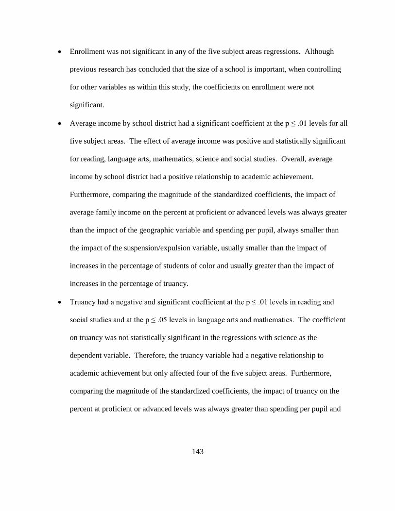
143

Enrollment was not significant in any of the five subject areas regressions. Although

previous research has concluded that the size of a school is important, when controlling

for other variables as within this study, the coefficients on enrollment were not

significant.

Average income by school district had a significant coefficient at the p ≤ .01 levels for all

five subject areas. The effect of average income was positive and statistically significant

for reading, language arts, mathematics, science and social studies. Overall, average

income by school district had a positive relationship to academic achievement.

Furthermore, comparing the magnitude of the standardized coefficients, the impact of

average family income on the percent at proficient or advanced levels was always greater

than the impact of the geographic variable and spending per pupil, always smaller than

the impact of the suspension/expulsion variable, usually smaller than the impact of

increases in the percentage of students of color and usually greater than the impact of

increases in the percentage of truancy.

Truancy had a negative and significant coefficient at the p ≤ .01 levels in reading and

social studies and at the p ≤ .05 levels in language arts and mathematics. The coefficient

on truancy was not statistically significant in the regressions with science as the

dependent variable. Therefore, the truancy variable had a negative relationship to

academic achievement but only affected four of the five subject areas. Furthermore,

comparing the magnitude of the standardized coefficients, the impact of truancy on the

percent at proficient or advanced levels was always greater than spending per pupil and

144

always smaller than the impact of the students of color and suspensions and expulsions

variables.

Lastly, disciplinary actions: suspensions and expulsions had a negative and significant

coefficient at the p ≤ .01 levels for all five-subject areas. Thus, increases in suspensions

and expulsions were associated with decreases in the percentage at the proficient or

advanced levels in reading, language arts, mathematics, science and social studies.

Therefore, suspensions and expulsions had a negative and statistically significant

relationship with academic achievement in all five subject areas. Furthermore,

comparing the magnitude of the standardized coefficients, the impact of suspensions and

expulsions on the percent at proficient or advanced levels was always greater than the

impact of the average income by school district, suburb, students of color, truancy and

spending per pupil variables.

The coefficient on the extra/co-curricular participation index was not statistically

significant in any regression within this study. Although the coefficients were never

significant, there is literature that exists stating participation in extra/co-curricular

activities is positively associated with student achievement. However, when controlling

for the effects of several other variables as within this study, the coefficient on the

extra/co-curricular participation index was not statistically significant in any of the five

subject area regressions.

In summary, the variables of students of color and disciplinary actions: suspensions and

expulsions had large and very statistically significant impact on the percentage of students at the

proficient or advanced levels in reading, language arts, mathematics, science and social studies.

145

Truancy also had an impact on four subject areas. High and positive correlations of the variables

percentage of students of color, percentages of suspensions and expulsions and percentages of

truancy existed with the geographic location variable City. Average income by school district

also illustrated a positive relationship to academic achievement in all five areas and spending per

pupil in two subject areas. Lastly, the effect of location in a suburb was positive and significant

in three subject areas, but the impact was small compared to other variables. Overall, geographic

location itself was not a strong predictor of academic achievement; however, the negative

strength of the variables students of color, disciplinary actions: suspensions and expulsions and

truancy influenced city schools substantially.

IMPLICATIONS

This study was intended to increase knowledge about the value of rural schools and to

provide useful information for policy makers and educational practitioners alike. Implications

for each of these groups follow.

Considering the findings of this study and the strength of the conclusions, one could

never argue that rural schools perform worse academically than town or city schools and should,

therefore, be consolidated. Indeed, neither city high schools nor town high schools outperformed

the rural schools. While the data suggest that suburban schools did better in some subject areas

than the other three locations, suburban schools did not outperform the other geographic location

types in all subject areas. Further, in the subject areas in which suburban performance was

statistically different, performance was only minimally better.

Previous researchers have identified a variety of benefits of rural schools to students,

families and communities. According to Hylden (2004),

146

Students in small schools perform better academically, graduate at higher levels, are more

likely to attend college, and earn higher salaries later on in life…they participate more in

extra-curricular activities, have better rates of attendance, report greater positive attitudes

towards learning, and are less likely to face school-related crime and violence…teachers

report greater job satisfaction, and are more likely to feel as if they are succeeding in their

work…parents and relatives are more likely to become involved in the school…small

schools are often characterized by personalized attention, curriculum integration and

specialization, relational trust and respect, a student sense of belonging, a strong positive

ethos, greater accountability, and a sense of communal mission (p. 3).

Hylden (2004) also suggested that communities benefit from small schools by having a central

meeting place for entertainment and activities, common advisory and decision-making practices

and a sense of pride.

Columbia University (Nachtigal, 1982) research showed that small schools had

“strengths of smallness” that were not apparent in large schools. Included in these strengths

were the number of students involved in extra-curricular activities, a higher number of students

in academic courses, a positive relationship between teachers and students due to teacher to

student ratio, and showing an appreciation and connection to their communities (Bard et al.,

2006).

Cotton (1996) listed eighteen core factors that students experienced attending a small

school. Among those eighteen core factors were academic achievement, attitude toward school,

social behavior problems, extracurricular participation, feeling of belongingness, interpersonal

relationships, attendance, dropout rates, self-concept, and success in college, etc. She further

147

stated from her analysis that the states with the larger schools and school districts had the lowest

achievement and social outcomes. Cotton (2001) states, “…small size alone is certainly not

enough…to improve the quality of schooling. What small size does is to provide an optimal

setting for high-quality schooling to take place” (p. 4).

Peshkin (1978, 1982) showed that schools serve as symbols of community autonomy,

vitality, tradition, and personal and community identity. Schools are generally a large employer

to a small community. They also create civic and social opportunities for citizens (Lyson, 2002).

From these studies, one can conclude small schools may provide more than just a positive

climate for education but also a core value and an identity to a community.

In 2002, O’Neal & Cox reviewed literature over a twenty year span and found small

school strengths within rural education that still seemed relevant today, including the following

examples:

Close relationships between faculty and administration

Less bureaucratic red tape

Decisions are more student-centered

A sense of community

More personal relationships between teachers and students

More favorable teacher to student ratios

Greater potential for individualized instruction

Allows for more student participation in extra/co-curricular activities

Fostering close relationships among teachers providing for a more unified staff

in vision and school mission

148

A greater opportunity for community partnerships

Increased parent involvement

Due to the fact that most of the high schools (54.9%) in Wisconsin are rural, that this

study demonstrated that Wisconsin rural schools performed as well as their city and town

counterparts in all subject areas of the tenth grade WKCE and as well as suburban districts in

two subject areas, and that the advantages to the community of having a local school are well-

documented, policy makers should make a commitment to make possible the long-term survival

of rural schools.

Educational practitioners should take special note of the findings of this study with

respect to the academic performance of students of color and of high schools with high

percentages of truancy and disciplinary actions: suspensions and expulsions. The data from this

study are clear and consistent with existing research: performance problems are prevalent for

students in certain demographic categories. The achievement gap widely written about and

highly discussed is real. A plethora of research exists on the importance of implementing

effective practices and doing so early in the life of risk students. Practitioners should implement

effective strategies in early elementary school so that achievement problems, which are more

difficult to remedy in later school years, never have a chance to develop.

LIMITATIONS OF THE STUDY

Several limitations existed within this study. First, two factors that the literature supports

as contributing to student achievement, student motivation and the relationship of the teacher to

students were excluded from this study because a quantifiable measure for each factor in

Wisconsin high schools did not exist. In addition, class size, according to some researchers, is

149

also a factor in student achievement, and it was not included in this study either. Class size was

not used as a variable due to the considerable disparity within a high school. For example, a

required class such as English may have 30 or more students while an advanced level language

class may have less than ten with both classes occurring within the same high school. Since

perhaps as much variation exists within a high school as between high schools in varying

locations and/or size, class size was not included as a factor in this study.

The base model used for data analysis (as defined in chapter 4) was highly explanatory

and did account for a large amount of variation among the variables, specifically reading (60%),

language arts (53.7%), mathematics (57.5%), science (60.6%) and social studies (59%).

Exclusion of the three previously mentioned variables did not appear to negatively impact the

findings.

Several other potential limitations of the study were identified. These limitations and

comments on their impact in the research follow:

1) Limitation: The use of school data rather than individual student test scores.

Comment: The results in the aggregate data paralleled very closely the research based on

data from individual student performance, so the ecological fallacy was not a problem in

this study.

2) Limitation: The use of school district data rather than high school data for average

income (parent education level) and spending per pupil.

Comment: Although school district data were only available for average income (parent

education level) and spending per pupil, it can be argued that both are general indicators

of the school district condition and are adequate descriptors of the high school (e.g. one

150

could argue that spending by school district per students would be similar across grades;

it is not likely that one district would spend ten times the amount on high school than

elementary and vice versa).

3) Limitation: The use of extra/co-curricular activity participation rates that included

grades 6-12.

Comment: Since the data were reported for grades 6-12 in all the schools in the study,

they are comparable data and appropriate for use in the research.

4) Limitation: The use of data on truancy, disciplinary actions: suspensions and

expulsions and extra/co-curricular participation were self-reported by the school

districts.

Comment: While it is possible to argue those school districts may define these variables

differently and, in some cases, more aggressively enforce these standards (i.e. truancy),

these data are the only data available. Other researchers who have studied truancy and

disciplinary actions have relied on self-reported data as well.

RECOMMENDATIONS

Based on the findings of this study, recommendations for future research and for data

collectors emerged.

One recommendation for additional research is to conduct a qualitative study examining

the role of student motivation and teacher relationship to student with respect to student

achievement. Such a case study, especially if it involved high schools in different geographic

location types, could add to the research base and shed additional light on the value of rural

schools on student achievement.

151

Another research recommendation is to conduct a quantitative study analyzing student

individual data versus school data by using standard scores or cut scores paired with individual

student background data. Since WDPI has a student location number for each student, one could

investigate what other individual data is tied to that number such as ethnicity, disability, truancy,

and the like.

A future possible research topic is a study including the new state test based on the

common core standards since WDPI appears to have plans to change the mandated state testing

program. Such a study would conceivably be more generalizable to other states and comparable

on a national level.

Recommendations for data collectors also emerged from this study. Data collectors

should compile individual student data (rather than district data) for performance on the WKCE

(and any other mandated state test in the future) and make it available through the WDPI.

Further, data that are currently collected and published should be cleaned so that they are

precisely what they are labeled to be. For example, if the WINSS system provides data for a

school labeled as a high school, then only data for grades 9-12 should be included and not other

grade level(s) (such as 6-12, 7-12, etc.). As noted previously, current data on WINSS, such as

the number of students participating in free and reduced lunch or the number of students with

disabilities, is listed as high school data but, in fact, includes data from other grade levels as well.

Further, NCES should be made aware that data provided by the WDPI might not be precisely as

it is labeled, and NCES should make appropriate notes for potential users of their data sources.

152

SUMMARY

In summary, rural high schools in the state of Wisconsin perform as well as town and city

high schools and in some subject areas as well as suburban high schools. The data analyses from

this study indicate that the argument that rural high schools should be consolidated because of

poor academic performance is not valid. Further, the data suggest that there are serious

academic performance concerns for students and schools with certain demographics and that

those problems need to be addressed immediately and effectively. All high schools in Wisconsin

including rural high schools should be supported by policy makers and practitioners to ensure

high academic achievement opportunities for all.

153

REFERENCES

Acharya, N., & Joshi, S. (2009). Influence of Parents' Education on Achievement Motivation of

Adolescents. Indian Journal Social Science Researches, 72-79.

Bailey, J. (2000). The Case for Small Schools. Walthill: Center for Rural Affairs.

Baker, M. L., Sigman, J. N., & Nugent, M. E. (2001). Truancy reduction: Keeping students in

school. Washington, D.C.: U.S. Department of Justice, Office of Juvenile Justice and

Delinquency Prevention.

Bard, J., Gardener, C., & Wieland, R. (2006). Rural School Consolidation: History, Research

Summary, Conclusions, and Recommendations. The Rural Educator, 40-48.

Baskerville, S. R., Duncan, J. M., & Hutchinson, F. E. (2010). How Do We Increase Attendance

and Student Success? Henniker: New England College.

Berry, C. (2004). School Inflation. Education Next, 56-58.

Bickel, R., & Howley, C. B. (2000). When It Comes to Schooling...Small Works: School Size,

Poverty, and Student Achievement. Randolph: Rural School and Community Trust.

Blasik, K. (2005). Student absences in Broward County public schools 1998-99 to first semester

2003-04. Fort Lauderdale: School Board of Broward County.

154

Blatchford, P., Bassett, P., & Brown, P. (2011). Examining the effect of class size on classroom

engagement and teacher-pupil interaction: Differences in relation to pupil prior

attainment and primary vs. secondary schools. Learning and Instruction, 715-730.

Cash, T., & Duttweiler, P. C. (2006). Planning, collaboration, and implementation: Strategies

for truancy programs. National Dropout Prevention Center.

Coffey, K. M., & Obringer, S. J. (2000). Culturally diverse rural students at special risk for LD

classification. Rural Special Education Quarterly, 1-20.

Connors, E. T. (1982). Educational funding and pupil achievement: The relationship between the

two variables. Richmond: Virginia State Department of Education.

Corwyn, R. F., & Bradley, R. F. (2002). Family Process Mediators of the Relation between SES

and Child Outcomes. Little Rock: University of Arkansas.

Cotton, K. (1996, December). Affective and Social Benefits of Small-Scale Schooling.

Charleston: ERIC Digest.

Cotton, K. (2001). New Small Learning Communities: Findings from Recent Literature.

Portland: Northwest Regional Educational Laboratory.

Crow, J. (2010). An Analysis of the Academic Achievement of Urban and Rural Low-

Socioeconomic Status Tennessee Public Schools. Ann Arbor: ProQuest LLC.

Davis-Kean, P. E. (2005). The Influence of Parent Education and Family Income on Child

Achievement: The Indirect Role of Parental Expectations and the Home Environment.

Journal of Family Psychology, 294-304.

155

De Haan, L. G., & MacDermid, S. (1998, Spring). The Relationship of Individual and Family

Factors to the Psychological Well-Being of Junior High Students Living in Urban

Poverty. Adolescence, pp. 73-89.

Debertin, D. L., & Goetz, S. J. (1994). Differences in Rural and Urban Schools: Issues for

Policymakers. Lexington: University of Kentucky, Department of Agricultural

Economics.

Dick, A. D. (2010). The Relationship of Participation in Extracurricular Activities to Student

Achievement, Student Attendance, and Student Behavior in a Nebraska School District.

Ann Arbor: UMI Dissertation Publishing.

Dillon, S. (2009, July 15). Racial Gap in Testing Sees Shift by Region. The New York Times.

Dynarksi, M., & Gleason, P. (1999). How Can We Help? Lessons From Federal Dropout

Prevention Programs. Princeton: Mathematica Policy Research, Inc.

Education Trust. (2003). Education Watch: Wisconsin. Key Facts and Figures. Achievement,

Attainment and Opportunity. From Elementary School through College. Washington,

D.C.: Education Trust.

Fan, X., & Chen, M. J. (1999). Academic Achievement of Rural School Students: A Multi-Year

Comparison with Their Peers in Suburban and Urban Schools. Journal of Research in

Rural Education, 31-46.

Fine, M., & Somerville, J. I. (1998). Small schools, big imaginations: A creative look at urban

public schools. Chicago: Cross city Campaign for Urban School Reform.

156

Friedkin, N., & Necochea, J. (1988). School system size and performance: A contingency

perspective. Educational Evaluation and Policy Analysis, 237-249.

Gehlbach, H., Brinkworth, M. E., & Harris, A. D. (2011). Social motivation in the secondary

classroom: Assessing teacher-student relationships from both perspectives. New Orleans:

Paper presented at the American Educational Research Association.

Haveman, R., & Wolfe, B. (1995). The determinants of children's attainments: A review of

methods and findings. Journal of Economic Literature, 1829-1878.

Hopkins, T. M. (2005). If You Are Poor, It is Better to be Rural: A Study of Mathematics

Achievement in Tennessee. The Rural Educator, 21-28.

Howley, C. B. (1989). Efficiency and the Characteristics of School Districts: A Study of 178

School Districts in Kentucky. Research in Rural Education, 33-43.

Howley, C. B. (1996). Sizing Up Schooling: A West Virginia Analysis and Critique.

Morgantown: West Virginia University.

Howley, C. B. (1999). The Matthew Project: State Report for Montana. Albany: Ohio University

and Appalachia Educational Laboratory.

Howley, C. B. (2000). School District Size and School Performance. Charleston: Rural

Education Issue Digest.

Huang, G., & Howley, C. (1993). Mitigating disadvantage: Effects of small-scale schooling on

students' achievement in Alaska. Journal of Research in Rural Education, 137-149.

157

Hylden, J. (2004). What's So Big About Small Schools? The Case for Small Schools: Nationwide

and in North Dakota. Cambridge: Harvard University.

Johnson, J. D., Howley, C. B., & Howley, A. A. (2002). Small Works in Arkansas: How Poverty

and the Size of Schools and School Districts Affect School Performance in Arkansas.

Washington D.C.: The Rural School and Community Trust.

Kennedy, R. (1990). Educational Indicators and Eighth Grade MPT Passing Rates. Hot Springs:

ERIC.

Klebanov, P. K., Brooks-Gunn, J., & Duncan, G. J. (1994). Does neighborhood and family

poverty affect mothers' parenting, mental health and social support? Journal of Marriage

and the Family, 441-455.

Klingele, W. E., & Warrick, B. K. (1990). Influence of cost and demographic factos on reading

achievement. Journal of Educational Research, 279-282.

Lee, V. E., & Smith, J. B. (1995). Effects of High School Restructuring and Size on Early Gains

in Achievement and Engagement. Sociology of Education, 241-270.

Lee, V. E., & Smith, J. B. (1997). High school size: Which works best, and for whom?

Eduational Evaluation and Policy Analysis, 205-227.

Lyson, T. A. (2002). What Does a School Mean to a Community? Assessing the Social and

Economic Benefits of Schools to Rural Villages in New York. Ithaca: Cornell University.

158

Martin, A. J., & Dowson, M. (2009). Interpersonal relationships, motivation, engagement, and

achievement: Yields for theory, current issues, and educational practice. Review of

Educational Research, 327-365.

McCluskey, C. P., Bynum, T., & Patchin, J. W. (2004). Reducing chronic absenteeism: An

assessment of an early truancy initiative. Crime & Delinquency, 214-234.

McCracken, J. D., & Barcinas, J. D. (1991). Differences Between Rural and Urban Schools,

Student Characteristics, and Student Aspirations in Ohio. Journal of Research in Rural

Education, 29-40.

McMullan, B. J., Sipe, C. L., & Wolf, W. C. (1994). Charters and Student Achievement: Early

Evidence from School Restructuring in Philadelphia. Cynwyd: Center for Assessment

and Policy Development.

Merriam-Webster. (2011). Merriam-Webster Dictionary. Retrieved June 15, 2011, from

Merriam-Webster Dictionary: http://www.merriam-webster.com/

Meyer, L. H., Weir, K. F., McClure, J., Walkey, F., & McKenzie, L. (2009, July). Motivation

and achievement at secondary school: The relationship between NCEA design and

student motivation and achievement: A three-year follow-up. Retrieved April 2, 2012,

from Education Counts: www.educationcounts.govt.nz/publications/schooling/50665

Nachtigal, P. (1982). In search of a better way. Boulder: Westview Press.

159

National Association of Secondary School Principals. (1996). Breaking ranks: Changing an

American institution. . Reston: National Association of Secondary School Principals and

Carnegie Foundation for the Advancement of Teaching.

National Federation of State High School Associations (NFHS). (2011). The Case for High

School Activities. Indianapolis: National Federation of State High School Associations

(NFHS).

Nitta, K. A., Holley, M. J., & Wrobel, S. L. (2010). A Phenomenological Study of Rural School

Consolidation. Journal of Research in Rural Education, 1-19.

Office of Management and Budget. (2000). Standards for Defining Metropolitan and

Micropolitan Statistical Areas. Washington D.C.: Federal Register.

O'Neal, L., & Cox, D. (2002). Then and Now: Small Rural Schools Revisited. Boone:

Appalachian State University.

Peshkin, A. (1978). Growing up american. Chicago: The University of Chicago Press.

Peshkin, A. (1982). The imperfect union: School consolidation and community conflict. Chicago:

The University of Chicago Press.

Purcell, D., & Shackelford, R. (2005). An evaluation of the impact of rural school consolidation:

What challenges may a new round of rural consolidation have on the 'safety, educational

performance and social environment' of rural communities? National Rural Education

Association.

160

Puzzanchera, C., Stahl, A., Finnegan, T., Snydeer, H., Poole, R., & Tierney, N. (2003).

Forthcoming: Juvenile court statistics report. Washington D.C.: U.S. Department of

Justice, Office of Juvenile Justice and Delinquency Prevention.

Rausch, M. K., & Skiba, R. (2004). Unplanned Outcomes: Suspensions and Expulsions in

Indiana. Bloomington: Center for Evaluation & Education Policy.

Rausch, M. K., & Skiba, R. J. (2006). The Academic Cost of Discipline: The Relationship

Between Suspension/Expulsion and School Achievement. Bloomington: Indiana

University Center for Evaluation and Education Policy.

Raywid, M. A. (1999, January). Current Literature on Small Schools. ERIC Clearinghouse on

Rural Education and Small Schools, 1-8.

Schmidt, J. K., & Lemke, M. (2006). How productive are southeastern Wisconsin schools?

Milwaukee: Public Policy Forum.

Schwinden, T. (1993). School Reorganization in Montana: A Time for Decision? Helena:

Montana School Boards Association.

Sharp, W. L. (1993). School Spending: Is There a Relationship between Spending and Student

Achievement? A Correlation Study of Illinois Schools. Carbondale: Southern Illinois

University.

Silverman, F. (2005, October). All Alone. Retrieved 05 19, 2011, from District Administration:

www.districtadministration.com

161

Smith, J. R., Brooks-Gunn, J., & Klebanov, P. K. (1997). Consequences of living in poverty for

young children's cognitive and verbal ability and early school achievement. New York:

Russell Sage Foundation.

StatSoft, Inc. (2011). Statistics Glossary. Retrieved January 21, 2012, from StatSoft Electronic

Statistics Textbook: http://www.statsoft.com/textbook/statistics-glossary/

Stein, J., Marley, P., & Berquist, L. (2011, March 1). Walker's budget cuts would touch most

Wisconsinites. Milwaukee, WI, USA.

Stewart, L. (2009). Achievement Differences between Large and Small Schools in Texas. The

Rural Educator, 20-28.

Sutton, J. M., & Pearson, R. (2002). The practice of school counseling in rural and small town

schools. Professional School Counseling, 266-276.

Swanson, P. C. (2008). Special Education in America: The state of students with disabilities in

the nation's high schools. Bethesda: Education Research Center.

Toch, T. (2003). High Schools on a Human Scale. Boston: Beacon Press.

United States Census Bureau. (2011, December 23). State & Country Quickfacts. Retrieved

January 21, 2012, from United States Census Bureau:

http://quickfacts.census.gov/qfd/states/55000.html

United States Department of Agriculture. (2011, November 30). Income Eligibility Guidelines.

Retrieved January 18, 2012, from Food and Nutrition Service:

http://www.fns.usda.gov/cnd/Governance/notices/iegs/IEGs.htm

162

United States Department of Agriculture Economic Research Service. (2007, September 4). Data

Sets. Retrieved January 17, 2012, from United States Department of Agriculture

Economic Research Service:

http://www.ers.usda.gov/data/ruraldefinitions/documentation.htm

United States Department of Education. (1998). Violence and Discipline Problems in U.S. Public

Schools: 1996-1997. Washington, D.C.: NCES.

United States Department of Education. (2001). Why Rural Matters: Common Core of Data,

Public School Universe. National Center for Education Statistics, 79-89.

United States Department of Education. (2008, October 19). Statistical Standards. Retrieved

January 18, 2012, from National Center for Education Statistics:

http://nces.ed.gov/statprog/2002/std1_5.asp

United States Department of Education. (2011). Search for Public Schools. Retrieved July 04,

2011, from National Center for Education Statistics: http://nces.ed.gov/ccd/schoolsearch/

United States Department of Education. (2012). National Center for Education Statistics.

Retrieved January 18, 2012, from School and District Glossary:

http://nces.ed.gov/ccd/commonfiles/glossary.asp

United States Department of Education. (2012, July 18). National Center for Education

Statistics. Retrieved from National Education Longitudinal Study of 1988 (NELS:88):

http://nces.ed.gov/surveys/nels88/

163

United States Department of Labor. (2011, November 17). Bureau of Labor Statistics. Retrieved

January 17, 2012, from Labor Force Statistics from the Current Population Survey:

www.bls.gov/cps/earnings.htm#education

Walberg, H., & Fowler, W. (1987). Expenditure and size efficiencies of public school districts.

Educational Researcher, 5-13.

Wendling, W., & Cohen, J. (1981). Education resources and student achievement: Good news

for schools. Journal of Education Finance, 44-63.

Wiederholt, M. (2009). Long-term effects of participation in high school athletics. Madison:

Edgewood College.

Williams, D. T. (1990). The Dimensions of Education: Recent Research on School Size.

Clemson: Strom Thurmond Institute of Government and Public Affairs.

Winters, J. J. (2003). An Examination of Eighth and Twelfth Grade Students' Mathematics

Achievement in Relation to School Locale, County Location, Looping Status, SES, Grade

and Class Size, and Access to Upper-Level Mathematics Courses in Tennessee. Ann

Arbor: ProQuest Information and Learning Company.

Wisconsin Department of Pubic Instruction. (2011, September 8). Department of Pubic

Instruction. Retrieved January 18, 2012, from Special Education Eligibility:

http://dpi.wi.gov/sped/eligibility.html

Wisconsin Department of Public Instruction. (2005). School Performance Report Data

Definitions and Directions. Madison: Wisconsin Department of Public Instruction.

164

Wisconsin Department of Public Instruction. (2009, July 1). WKCE Proficiency Score Ranges.

Retrieved January 18, 2012, from Office of Educational Accountability:

http://dpi.wi.gov/oea/wkce-crtcuts.html

Wisconsin Department of Public Instruction. (2010). WKCE Fall 2009 Technical Manual.

Madison, WI, USA.

Wisconsin Department of Public Instruction. (2011, December 15). Wisconsin Department of

Public Instruction. Retrieved January 18, 2012, from Understanding Habitual Truancy

Data: http://dpi.wi.gov/spr/tru_q&a.html#definitions

Wisconsin Department of Public Instruction. (2011, December 21). Wisconsin Department of

Public Instruction. Retrieved January 18, 2012, from Race and Ethnicity Data Collection

FAQ: http://dpi.wi.gov/lbstat/dataracfaq.html

Wisconsin Department of Public Instruction. (2012, February 13). Public School Enrollment

Data. Retrieved March 31, 2012, from Wisconsin Department of Public Instruction:

http://dpi.wi.gov/lbstat/pubdata2.html

Wisconsin Department of Public Instruction. (2012). Wisconsin Information Network for

Successful Schools (WINSS). Retrieved March 1, 2012, from Wisconsin Information

Network for Successful Schools (WINSS): http://dpi.wi.gov/sig/index.html

Wisconsin Department of Public Instruction. (n.d.). School Finance Data Warehouse Home.

Retrieved January 18, 2012, from School Finance Data Warehouse:

http://www2.dpi.state.wi.us/sfsdw/Std_Rpts.asp

165

Wisconsin Department of Revenue. (2011, November 25). Reports - I. Retrieved January 18,

2012, from Wisconsin Department of Revenue: http://www.revenue.wi.gov/report/i.html

166

APPENDIX A

104 HIGH SCHOOLS

(not included in free and reduced lunch participation and students with disabilities variables)

Abbotsford Algoma Almond

Argyle Auburndale Augusta

Bangor Barneveld Pembine

Belleville Belmont Benton

Blair-Taylor Bowler Boyceville

Bruce Butternut Cambria-Friesland

Cameron Cashton Cassville

Cedar Grove Cochrane-Fountain City Colby

Coleman Colfax Cornell

Dodgeland Durand Eleva-Strum

Elmbrook East Fall River Fennimore

Frederic Gilman Gilmanton

Goodman Green Lake Greenwood

Gresham Highland Hilbert

Hillsboro Hurley Hustisford

Independence Iola-Scandinavia Jefferson

Johnson Creek Kickapoo Kohler

La Farge Laona Luck

Little Wolf Marion Menominee

Mercer Milwaukee School of the

Languages

Northwest Secondary

School

Mishicot Monroe Montello

Necedah Neillsville New Auburn

New Berlin Eisenhower New Berlin High New Glarus

New Lisbon Niagara Norris

North Crawford Northwood Norwalk-Ontario-Wilton

Brookwood

Oakfield Pecatonica Pepin

Peshtigo Plum City Potosi

Prescott Princeton Rio

Royall Sheboygan Falls Shell Lake

Siren Slinger Solon Springs

Somerset South Shore Spencer

Stratford Three Lakes Tigerton

Tri-County Turtle Lake Wabeno

Waterloo Wautoma Wauzeka

White Lake Wild Rose

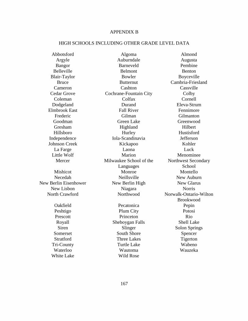
167

APPENDIX B

HIGH SCHOOLS INCLUDING OTHER GRADE LEVEL DATA

Abbotsford Algoma Almond

Argyle Auburndale Augusta

Bangor Barneveld Pembine

Belleville Belmont Benton

Blair-Taylor Bowler Boyceville

Bruce Butternut Cambria-Friesland

Cameron Cashton Cassville

Cedar Grove Cochrane-Fountain City Colby

Coleman Colfax Cornell

Dodgeland Durand Eleva-Strum

Elmbrook East Fall River Fennimore

Frederic Gilman Gilmanton

Goodman Green Lake Greenwood

Gresham Highland Hilbert

Hillsboro Hurley Hustisford

Independence Iola-Scandinavia Jefferson

Johnson Creek Kickapoo Kohler

La Farge Laona Luck

Little Wolf Marion Menominee

Mercer Milwaukee School of the

Languages

Northwest Secondary

School

Mishicot Monroe Montello

Necedah Neillsville New Auburn

New Berlin Eisenhower New Berlin High New Glarus

New Lisbon Niagara Norris

North Crawford Northwood Norwalk-Ontario-Wilton

Brookwood

Oakfield Pecatonica Pepin

Peshtigo Plum City Potosi

Prescott Princeton Rio

Royall Sheboygan Falls Shell Lake

Siren Slinger Solon Springs

Somerset South Shore Spencer

Stratford Three Lakes Tigerton

Tri-County Turtle Lake Wabeno

Waterloo Wautoma Wauzeka

White Lake Wild Rose

168

APPENDIX C

OUTLIER SCATTER PLOTS

1. Socioeconomic Status (free and reduced lunch):

2. Students of Color:

169

3. Spending per Pupil:

4. High School Enrollment:

170

5. Parent Education Level (Average Income by School District):

6. Truancy:

171

7. Suspensions & Expulsions:

8. Students with Disabilities:

172

9. Extra/Co-curricular Participation Index:

173

APPENDIX D

FACTOR_1 & FACTOR_2 COMPONENT MATRIX

Component Matrixa

Component

1 2

Students_Color_Per .868 .318

Income_1000 -.567 .798

FRRL_Per .872 -.387

Truancy_Per .880 .273

Sum_Sus_Exp .863 .315

Extraction Method: Principal Component

Analysis.

a. 2 components extracted.

student academic achievement in rural

Documents

Transcript of student academic achievement in rural