Linear Matrix Inequalities in Control
60
1/54 Linear Matrix Inequalities in Control Carsten Scherer Delft Center for Systems and Control (DCSC) Delft University of Technology The Netherlands Siep Weiland Department of Electrical Engineering Eindhoven University of Technology The Netherlands
Transcript of Linear Matrix Inequalities in Control

1/54
Linear Matrix Inequalities in Control
Carsten Scherer
Delft Center for Systems and Control (DCSC)
Delft University of Technology
The Netherlands
Siep Weiland
Department of Electrical Engineering
Eindhoven University of Technology
The Netherlands
Optimization and Control
2/54
Carsten Scherer Siep Weiland
Classically optimization and control are highly intertwined:
• Optimal control (Pontryagin/Bellman)
• LQG-control or H2-control
• H∞-synthesis and robust control
• Model Predictive Control
Main Theme
View control input signal and/or feedback controller as decision
variable of an optimization problem.
Desired specs are imposed as constraints on controlled system.
Sketch of Issues
3/54
Carsten Scherer Siep Weiland
• How to distinguish easy from difficult optimization problems?
• What are the consequences of convexity in optimization?
• What is robust optimization?
• Which performance measures can be incorporated?
• How can controller synthesis be convexified?
• How can we check robustness by convex optimization?
• What are the limits for the synthesis of robust controllers?
• How can we perform systematic gain-scheduling?
Outline
3/54
Carsten Scherer Siep Weiland
• From Optimization to Convex Semi-Definite Programming
• Convex Sets and Convex Functions
• Linear Matrix Inequalities (LMIs)
• Truss-Topology Design
• LMIs and Stability
• A First Glimpse at Robustness
Optimization
4/54
Carsten Scherer Siep Weiland
The ingredients of any optimization problem are:
• A universe of decisions x ∈ X
• A subset S ⊂ X of feasible decisions
• A cost function or objective function f : S → R
Optimization Problem/Programming Problem
Find a feasible decision x ∈ S with the least possible cost f(x).
In short such a problem is denoted as
minimize f(x)
subject to x ∈ S

Questions in Optimization
5/54
Carsten Scherer Siep Weiland
• What is the least possible cost? Compute the optimal value
fopt := infx∈S
f(x) ≥ −∞.
Convention: If S = ∅ then fopt = +∞.
If fopt = −∞ the problem is said to be unbounded from below.
• How can we compute almost optimal solutions? For any chosen
positive absolute error ε, determine
xε ∈ S with fopt ≤ f(xε) ≤ fopt + ε.
By definition of the infimum such an xε does exist for all ε > 0.

Questions in Optimization
6/54
Carsten Scherer Siep Weiland
• Is there an optimal solution? Does there exist
xopt ∈ S with f(xopt) = fopt?
If yes, the minimum is attained and we write
fopt = minx∈S
f(x).
Set of all optimal solutions is denoted as
arg minx∈S
f(x) = {x ∈ S : f(x) = fopt}.
• Is optimal solution unique?

Recap: Infimum and Minimum of Functions
7/54
Carsten Scherer Siep Weiland
Any f : S → R has infimum l ∈ R ∪ {−∞} denoted as infx∈S f(x).
The infimum is uniquely defined by the following properties:
• l ≤ f(x) for all x ∈ S.
• l finite: For all ε > 0 exists x ∈ S with f(x) ≤ l + ε.
l = −∞: For all ε > 0 exists x ∈ S with f(x) ≤ −ε.
If there exists x0 ∈ S with f(x0) = infx∈S f(x) we say that f attains
its minimum on S and write l = minx∈S f(x).
If existing the minimum is uniquely defined through the properties:
• l ≤ f(x) for all x ∈ S.
• There exists some x0 ∈ S with f(x0) = l.

Nonlinear Programming (NLP)
8/54
Carsten Scherer Siep Weiland
With decision universe X = Rn, the feasible set S is often defined by
constraint functions g1 : X → R, . . . , gm : X → R as
S = {x ∈ X : g1(x) ≤ 0, . . . , gm(x) ≤ 0} .
The general nonlinear optimization problem is formulated as
minimize f(x)
subject to x ∈ X , g1(x) ≤ 0, . . . , gm(x) ≤ 0.
By exploiting particular properties of f, g1, . . . , gm (e.g. smoothness),
optimization algorithms typically allow to iteratively compute locally
optimal solutions x0: There exists an ε > 0 such that x0 is optimal on
S ∩ {x ∈ X : ‖x− x0‖ ≤ ε}.

Example: Quadratic Program
9/54
Carsten Scherer Siep Weiland
f : Rn → R is quadratic iff there exists a symmetric matrix P with
f(x) =
(1
x
)T
P
(1
x
).
Quadratically constrained quadratic program
minimize
(1
x
)T
P0
(1
x
)
subject to x ∈ Rn,
(1
x
)T
Pk
(1
x
)≤ 0, k = 1, . . . ,m
where P0, P1, . . . , Pm ∈ Sn+1.
Linear Programming (LP)
10/54
Carsten Scherer Siep Weiland
With the decision vectors x = (x1 · · · xn)T ∈ Rn consider the problem
minimize c1x1 + · · ·+ cnxn
subject to a11x1 + · · ·+ a1nxn ≤ b1
...
am1x1 + · · ·+ amnxn ≤ bm
The cost is linear and the set of feasible decisions is defined by finitely
many affine inequality constraints.
Simplex algorithms or interior point methods allow to efficiently
1. decide whether the constraint set is feasible (value < ∞).
2. decide whether problem is bounded from below (value > −∞).
3. compute an (always existing) optimal solution if 1. & 2. are true.

Linear Programming (LP)
11/54
Carsten Scherer Siep Weiland
Major early contributions in 1940s by
• George Dantzig (simplex method)
• John von Neumann (duality)
• Lenoid Kantorovich (economics applications)
Leonid Khachiyan proved polynomial-time solvability in 1979.
Narendra Karmakar introduce an interior point method in 1984.
Has numerous applications for example in economical planning problems
(business management, flight-scheduling, resource allocation, finance).
LPs have spurred the development of optimization theory and appear
as subproblem in many optimization algorithms.
Recap
12/54
Carsten Scherer Siep Weiland
For a real or complex matrix A the inequality A 4 0 means that A
is Hermitian and negative semi-definite.
• A is defined to be Hermitian if A = A∗ = AT . If A is real then this
amounts to A = AT and A is then called symmetric.
All eigenvalues of Hermitian matrices are real.
• By definition A is negative semi-definite if A = A∗ and
x∗Ax ≤ 0 for all complex vectors x 6= 0.
A is negative semi-definite iff all its eigenvalues are non-positive.
• A 4 B means by definition: A, B are Hermitian and A−B 4 0.
• A ≺ B, A 4 B, A < B, A � B defined/characterized analogously.

Recap
13/54
Carsten Scherer Siep Weiland
Let A be partitioned with square diagonal blocks as
A =
A11 · · · A1m
.... . .
...
Am1 · · · Amm
.
Then
A ≺ 0 implies A11 ≺ 0, . . . , Amm ≺ 0.
Prototypical Proof. Choose any vector zi 6= 0 of length compatible
with the size of Aii. Define z = (0, . . . , 0, zTi , 0, . . . , 0)T 6= 0 with the
zeros blocks compatible in size with A11, . . . , Amm. This construction
implies zT Az = zTi Aiizi. Since A ≺ 0, we infer zT Az < 0. Therefore,
zTi Aiizi < 0. Since zi 6= 0 was arbitrary we infer Aii ≺ 0.

Semi-Definite Programming (SDP)
14/54
Carsten Scherer Siep Weiland
Let us now assume that the constraint functions G1, . . . , Gm map Xinto the set of symmetric matrices, and define the feasible set S as
S = {x ∈ X : G1(x) 4 0, . . . , Gm(x) 4 0} .
The general semi-definite program (SDP) is formulated as
minimize f(x)
subject to x ∈ X , G1(x) 4 0, . . . , Gm(x) 4 0.
• This includes NLPs as a special case.
• Is called convex if f and G1, . . . , Gm are convex.
• Is called linear matrix inequality (LMI) optimization problem
or linear SDP if f and G1, . . . , Gm are affine.

Outline
14/54
Carsten Scherer Siep Weiland
• From Optimization to Convex Semi-Definite Programming
• Convex Sets and Convex Functions
• Linear Matrix Inequalities (LMIs)
• Truss-Topology Design
• LMIs and Stability
• A First Glimpse at Robustness
Recap: Affine Sets and Functions
15/54
Carsten Scherer Siep Weiland
The set S in the vector space X is affine if
λx1 + (1− λ)x2 ∈ S for all x1, x2 ∈ S, λ ∈ R.
The matrix-valued function F defined on S is affine if the domain
of definition S is affine and if
F (λx1 + (1− λ)x2) = λF (x1) + (1− λ)F (x2)
for all x1, x2 ∈ S, λ ∈ R.
For points x1, x2 ∈ S recall that
• {λx1 + (1− λ)x2 : λ ∈ R} is the line through x1, x2
• {λx1 + (1− λ)x2 : λ ∈ [0, 1]} is the line segment between x1, x2
Recap: Convex Sets and Functions
16/54
Carsten Scherer Siep Weiland
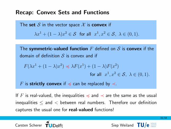
The set S in the vector space X is convex if
λx1 + (1− λ)x2 ∈ S for all x1, x2 ∈ S, λ ∈ (0, 1).
The symmetric-valued function F defined on S is convex if the
domain of definition S is convex and if
F (λx1 + (1− λ)x2) 4 λF (x1) + (1− λ)F (x2)
for all x1, x2 ∈ S, λ ∈ (0, 1).
F is strictly convex if 4 can be replaced by ≺.
If F is real-valued, the inequalities 4 and ≺ are the same as the usual
inequalities ≤ and < between real numbers. Therefore our definition
captures the usual one for real-valued functions!
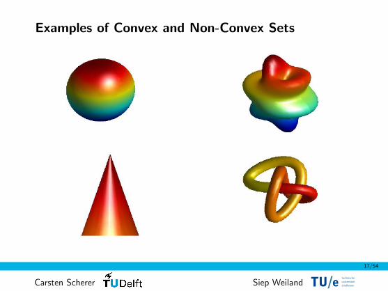
Examples of Convex and Non-Convex Sets
17/54
Carsten Scherer Siep Weiland
Examples of Convex Sets
18/54
Carsten Scherer Siep Weiland
The intersection of any family of convex sets is convex.
• With a ∈ Rn \ {0} and b ∈ R, the hyperplane {x ∈ Rn : aT x = b}is affine while the half-space {x ∈ Rn : aT x ≤ b} is convex.
• The intersection of finitely many hyperplanes and half-planes defines
a polyhedron. Any polyhedron is convex and can be described as
{x ∈ Rn : Ax ≤ b, Dx = e}
with suitable matrices A, D, vectors b, e. A compact polyhedron is
said to be a polytope.
• The set of negative semi-definite/negative definite matrices is convex.
Convex Combination and Convex Hull
19/54
Carsten Scherer Siep Weiland
• x ∈ X is convex combination of x1, ..., xl ∈ X if
x =l∑
k=1
λkxk with λk ≥ 0,
l∑k=1
λk = 1.
Convex combination of a convex combination is a convex combination.
• The convex hull co(S) of any subset S ⊂ X is defined in one of the
following equivalent fashions:
1. Set of all convex combinations of points in S.
2. Intersection of all convex sets that contain S.
For arbitrary S the convex hull co(S) is convex.

Explict Description of Polytopes
20/54
Carsten Scherer Siep Weiland
Any point in the convex hull of the finite set {x1, . . . , xl} is given by a
(not necessarily unique) convex combination of generators x1, . . . , xl.
The convex hull of finitely many points co{x1, . . . , xl} is a polytope.
Any polytope can be represented in this way.
In this fashion one can explicitly describe polytopes, in contrast to an
implicit description such as {x ∈ Rn : Ax ≤ b}. Note that the implicit
description is often preferable for reasons of computational complexity.
Example: {x ∈ Rn : a ≤ x ≤ b} is defined by 2n inequalities but
requires 2n generators for its description as a convex hull.

Examples of Convex and Non-Convex Functions
21/54
Carsten Scherer Siep Weiland

On Checking Convexity of Functions
22/54
Carsten Scherer Siep Weiland
All real-valued or Hermitian-valued affine functions are convex.
It is often not simple to verify whether a non-affine function is convex.
The following fact (for S ⊂ Rn with interior points) might help.
The C2-map f : S → R is convex iff ∂2f(x) < 0 for all x ∈ S.
It is not easy to find convexity tests for Hermitian-valued function in the
literature. The following reduction to real-valued functions often helps.
The Hermitian-valued map F defined on S is convex iff
S 3 x → z∗F (x)z ∈ R
is convex for all complex vectors z ∈ Cm.

Convex Constraints
23/54
Carsten Scherer Siep Weiland
Suppose that F defined on S is convex. For all Hermitian H the
strict or non-strict sub-level sets
{x ∈ S : F (x) ≺ H} and {x ∈ S : F (x) 4 H}
“of level H” are convex.
Note that the converse is in general not true!
• The feasible set of the convex SDP on slide 13 is convex.
• Convex sets are typically described as the finite intersection of such
sub-level sets. If the involved functions are even affine this is often
called an LMI representation.
• Convexity is necessary for a set to have an LMI representation.
Example: Quadratic Functions
24/54
Carsten Scherer Siep Weiland
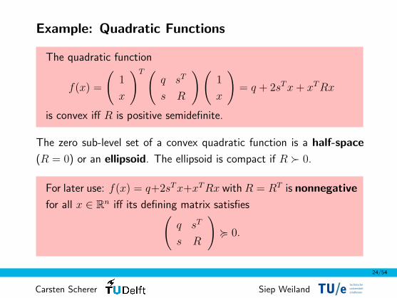
The quadratic function
f(x) =
(1
x
)T (q sT
s R
)(1
x
)= q + 2sT x + xT Rx
is convex iff R is positive semidefinite.
The zero sub-level set of a convex quadratic function is a half-space
(R = 0) or an ellipsoid. The ellipsoid is compact if R � 0.
For later use: f(x) = q+2sT x+xT Rx with R = RT is nonnegative
for all x ∈ Rn iff its defining matrix satisfies(q sT
s R
)< 0.

Important Properties
25/54
Carsten Scherer Siep Weiland
Property 1: Jensen’s Inequality.
If F defined on S is convex then for all x1, . . . , xl ∈ S and λ1, . . . , λl ≥ 0
with λ1 + · · ·+ λl = 1 we infer λ1x1 + · · ·+ λlx
l ∈ S and
F (λ1x1 + · · ·+ λlx
l) 4 λ1F (x1) + · · ·+ λlF (xl).
Source of many inequalities in mathematics! Proof: cc of cc is cc!
Property 2. If F and G define on S are convex then F + G and αF
for α ≥ 0 as well as
S 3 x → λmax(F (x)) ∈ R
are all convex. If F and G are scalar-valued then max{F, G} is convex.
There are many other operations for functions that preserve convexity.
A Key Consequence
26/54
Carsten Scherer Siep Weiland
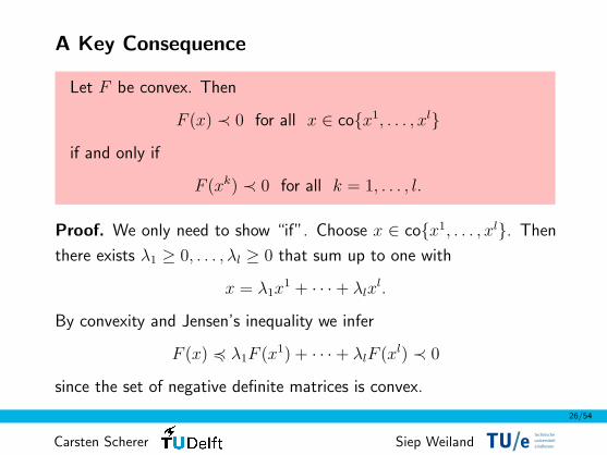
Let F be convex. Then
F (x) ≺ 0 for all x ∈ co{x1, . . . , xl}
if and only if
F (xk) ≺ 0 for all k = 1, . . . , l.
Proof. We only need to show “if”. Choose x ∈ co{x1, . . . , xl}. Then
there exists λ1 ≥ 0, . . . , λl ≥ 0 that sum up to one with
x = λ1x1 + · · ·+ λlx
l.
By convexity and Jensen’s inequality we infer
F (x) 4 λ1F (x1) + · · ·+ λlF (xl) ≺ 0
since the set of negative definite matrices is convex.

General Remarks on Convex Programs
27/54
Carsten Scherer Siep Weiland
• Solvers for general nonlinear programs typically determine local op-
timal solutions. There are no guarantees for global optimality.
• Main feature of convex programs:
Locally optimal solutions are globally optimal.
Convexity alone neither guarantees that the optimal value is finite,
nor that there exists an optimal solution/efficient solution algorithms.
• In general convex programs can be solved with guarantees on accuracy
if one can compute (sub)gradients of objective/constraint functions.
• Strictly feasible linear semi-definite programs are convex and can be
solved very efficiently, with guarantees on accuracy at termination.

Outline
27/54
Carsten Scherer Siep Weiland
• From Optimization to Convex Semi-Definite Programming
• Convex Sets and Convex Functions
• Linear Matrix Inequalities (LMIs)
• Truss-Topology Design
• LMIs and Stability
• A First Glimpse at Robustness
Linear Matrix Inequalities (LMIs)
28/54
Carsten Scherer Siep Weiland
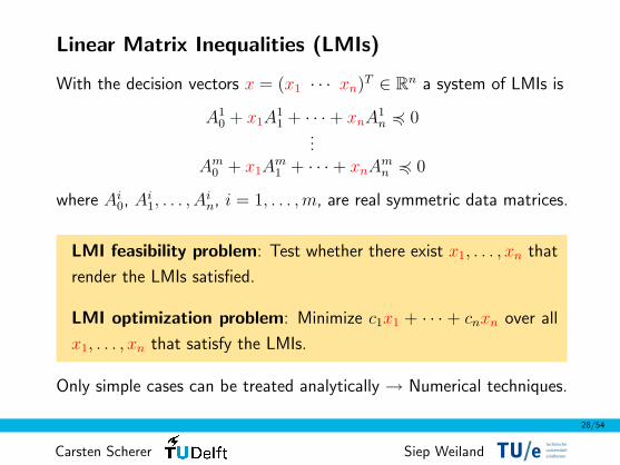
With the decision vectors x = (x1 · · · xn)T ∈ Rn a system of LMIs is
A10 + x1A
11 + · · ·+ xnA
1n 4 0
...Am
0 + x1Am1 + · · ·+ xnA
mn 4 0
where Ai0, Ai
1, . . . , Ain, i = 1, . . . ,m, are real symmetric data matrices.
LMI feasibility problem: Test whether there exist x1, . . . , xn that
render the LMIs satisfied.
LMI optimization problem: Minimize c1x1 + · · · + cnxn over all
x1, . . . , xn that satisfy the LMIs.
Only simple cases can be treated analytically → Numerical techniques.

LMI Optimization Problems
29/54
Carsten Scherer Siep Weiland
minimize c1x1 + · · ·+ cnxn
subject to Ai0 + x1A
i1 + · · ·+ xnA
in 4 0, i = 1, . . . ,m
• Natural generalization of LPs with inequalities defined by the cone of
positive semi-definite matrices. Considerable richer class than LPs.
• The i-th constraint can be equivalently expressed as
λmax(Ai0 + x1A
i1 + · · ·+ xnA
in) ≤ 0.
• Interior-point or bundle methods allow to effectively decide about
feasibility/boundedness and to determine almost optimal solutions.
• Must be strictly feasible: There exists some decision x for which
the constraint inequalities are strictly satisfied.
Testing Strict Feasbility
30/54
Carsten Scherer Siep Weiland
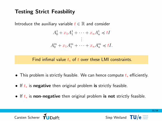
Introduce the auxiliary variable t ∈ R and consider
A10 + x1A
11 + · · ·+ xnA
1n 4 tI
...Am
0 + x1Am1 + · · ·+ xnA
mn 4 tI.
Find infimal value t∗ of t over these LMI constraints.
• This problem is strictly feasible. We can hence compute t∗ efficiently.
• If t∗ is negative then original problem is strictly feasible.
• If t∗ is non-negative then original problem is not strictly feasible.
LMI Optimization Problems
31/54
Carsten Scherer Siep Weiland
Developments
• Bellman/Fan initialized derivation of optimality conditions (1963)
• Jan Willems coined terminology LMI and revealed relation to dissi-
pative dynamical systems (1971/72)
• Nesterov/Nemirovski exhibited essential feature (self-concordance)
for existence of polynomial-time solution algorithm (1988)
• Interior-point methods: Alizadeh (1992), Kamath/Karmarkar (1992)
Suggested books: Boyd/El Ghaoui (1994), El Ghaoui/Niculescu (2000),
Ben-Tal/Nemiorvski (2001), Boyd/Vandenberghe (2004)
What are LMIs good for?
32/54
Carsten Scherer Siep Weiland
• Many engineering optimization problem can be (often but not always
easily) translated into LMI problems.
• Various computationally difficult optimization problems can be effec-
tively approximated by LMI problems.
• In practice the description of the data is affected by uncertainty.
Robust optimization problems can be handled/approximated by
standard LMI problems.
In this course
How can we solve (robust) control problems with LMIs?

Outline
32/54
Carsten Scherer Siep Weiland
• From Optimization to Convex Semi-Definite Programming
• Convex Sets and Convex Functions
• Linear Matrix Inequalities (LMIs)
• Truss-Topology Design
• LMIs and Stability
• A First Glimpse at Robustness

Truss Topology Design
33/54
Carsten Scherer Siep Weiland
0 50 100 150 200 250 300 350 400
0
50
100
150
200
250

Example: Truss Topology Design
34/54
Carsten Scherer Siep Weiland
• Connect nodes with N bars of length l = col(l1, . . . , lN) (fixed) and
cross-sections x = col(x1, . . . , xN) (to-be-designed).
• Impose bounds ak ≤ xk ≤ bk on cross-section and lT x ≤ v on total
volume (weight). Abbreviate a = col(a1, . . . , aN), b = col(b1, . . . , bN).
• If applying external forces f = col(f1, . . . , fM) (fixed) on nodes the
construction reacts with the node displacement d = col(d1, . . . , dM).
Mechanical model: A(x)d = f where A(x) is the stiffness matrix
which depends linearly on x and has to be positive semi-definite.
• Goal is to maximize stiffness, for example by minimizing the elastic
stored energy fT d.

Example: Truss Topology Design
35/54
Carsten Scherer Siep Weiland
Find x ∈ RN which minimizes fT d subject to the constraints
A(x) < 0, A(x)d = f, lT x ≤ v, a ≤ x ≤ b.
Features
• Data: Scalar v, vectors f , a, b, l, and symmetric matrices A1, . . . , AN
which define the linear mapping A(x) = A1x1 + · · ·+ ANxN .
• Decision variables: Vectors x and d.
• Objective function: d → fT d which happens to be linear.
• Constraints: Semi-definite constraint A(x) < 0, nonlinear equality
constraint A(x)d = f , and linear inequality constraints lT x ≤ v,
a ≤ x ≤ b. Latter interpreted elementwise!
From Truss Topology Design to LMI’s
36/54
Carsten Scherer Siep Weiland
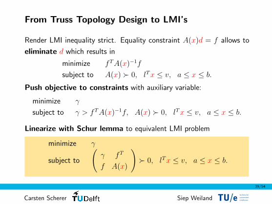
Render LMI inequality strict. Equality constraint A(x)d = f allows to
eliminate d which results in
minimize fT A(x)−1f
subject to A(x) � 0, lT x ≤ v, a ≤ x ≤ b.
Push objective to constraints with auxiliary variable:
minimize γ
subject to γ > fT A(x)−1f, A(x) � 0, lT x ≤ v, a ≤ x ≤ b.
Trouble: Nonlinear inequality constraint γ > fT A(x)−1f .

Recap: Congruence Transformations
37/54
Carsten Scherer Siep Weiland
Given a Hermitian matrix A and a square non-singular matrix T ,
A → T ∗AT
is called a congruence transformation of A.
If T is square and non-singular then
A ≺ 0 if and only if T ∗AT ≺ 0.
The following more general statement is also easy to remember.
If A is Hermitian and T is nonsingular, the matrices A and T ∗AT
have the same number of negative, zero, positive eigenvalues.
What is true if T is not square? ... if T has full column rank?
Recap: Schur-Complement Lemma
38/54
Carsten Scherer Siep Weiland
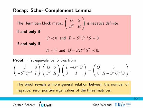
The Hermitian block matrix
(Q S
ST R
)is negative definite
if and only if
Q ≺ 0 and R− ST Q−1S ≺ 0
if and only if
R ≺ 0 and Q− SR−1ST ≺ 0.
Proof. First equivalence follows from(I 0
−ST Q−1 I
)(Q S
ST R
)(I −Q−1S
0 I
)=
(Q 0
0 R− ST Q−1S
).
The proof reveals a more general relation between the number of
negative, zero, positive eigenvalues of the three matrices.
From Truss Topology Design to LMI’s
39/54
Carsten Scherer Siep Weiland
Render LMI inequality strict. Equality constraint A(x)d = f allows to
eliminate d which results in
minimize fT A(x)−1f
subject to A(x) � 0, lT x ≤ v, a ≤ x ≤ b.
Push objective to constraints with auxiliary variable:
minimize γ
subject to γ > fT A(x)−1f, A(x) � 0, lT x ≤ v, a ≤ x ≤ b.
Linearize with Schur lemma to equivalent LMI problem
minimize γ
subject to
(γ fT
f A(x)
)� 0, lT x ≤ v, a ≤ x ≤ b.

Yalmip-Coding: Truss Toplogy Design
40/54
Carsten Scherer Siep Weiland
minimize γ
subject to
(γ fT
f A(x)
)� 0, lT x ≤ v, a ≤ x ≤ b.
Suppose A(x)=∑N
k=1 xkmkmTk with vectors mk collected in matrix M .
The following code with Yalmip commands solves LMI problem:
gamma=sdpvar(1,1); x=sdpvar(N,1,’full’);
lmi=set([gamma f’;f M*diag(x)*M’]);
lmi=lmi+set(l’*x<=v);
lmi=lmi+set(a<=x<=b);
options=sdpsettings(’solver’,’sedumi’);
solvesdp(lmi,gamma,options); s=double(x);
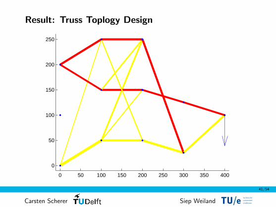
Result: Truss Toplogy Design
41/54
Carsten Scherer Siep Weiland
0 50 100 150 200 250 300 350 400
0
50
100
150
200
250

Quickly Accessible Software
42/54
Carsten Scherer Siep Weiland
General purpose Matlab interface Yalmip:
• Free code developed by J. Lofberg and accessible at
http://control.ee.ethz.ch/~joloef/yalmip.msql
• Can use usual Matlab-syntax to define optimization problem.
Is extremely easy to use and very versatile. Highly recommended!
• Provides access to a whole suite of public and commercial optimiza-
tion solvers, including fastest available dedicated LMI-solvers.
Matlab LMI-Toolbox for dedicated control applications. Has recently
been integrated into new Robust Control Toolbox.

Outline
42/54
Carsten Scherer Siep Weiland
• From Optimization to Convex Semi-Definite Programming
• Convex Sets and Convex Functions
• Linear Matrix Inequalities (LMIs)
• Truss-Topology Design
• LMIs and Stability
• A First Glimpse at Robustness
General Formulation of LMI Problems
43/54
Carsten Scherer Siep Weiland
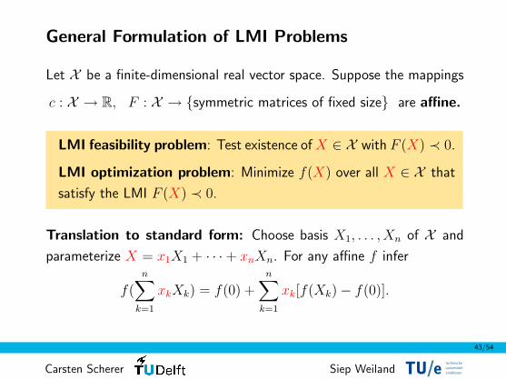
Let X be a finite-dimensional real vector space. Suppose the mappings
c : X → R, F : X → {symmetric matrices of fixed size} are affine.
LMI feasibility problem: Test existence of X ∈ X with F (X) ≺ 0.
LMI optimization problem: Minimize f(X) over all X ∈ X that
satisfy the LMI F (X) ≺ 0.
Translation to standard form: Choose basis X1, . . . , Xn of X and
parameterize X = x1X1 + · · ·+ xnXn. For any affine f infer
f(n∑
k=1
xkXk) = f(0) +n∑
k=1
xk[f(Xk)− f(0)].
Diverse Remarks
44/54
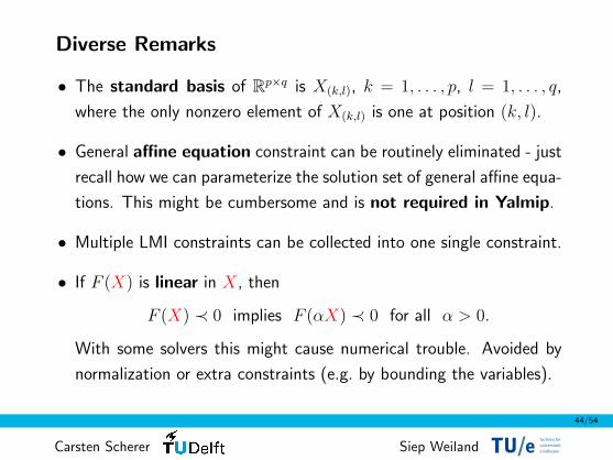
Carsten Scherer Siep Weiland
• The standard basis of Rp×q is X(k,l), k = 1, . . . , p, l = 1, . . . , q,
where the only nonzero element of X(k,l) is one at position (k, l).
• General affine equation constraint can be routinely eliminated - just
recall how we can parameterize the solution set of general affine equa-
tions. This might be cumbersome and is not required in Yalmip.
• Multiple LMI constraints can be collected into one single constraint.
• If F (X) is linear in X, then
F (X) ≺ 0 implies F (αX) ≺ 0 for all α > 0.
With some solvers this might cause numerical trouble. Avoided by
normalization or extra constraints (e.g. by bounding the variables).

Example: Spectral Norm Approximation
45/54
Carsten Scherer Siep Weiland
For real data matrices A, B, C and some unknown X consider
minimize ‖AXB − C‖subject to X ∈ S
where S is a matrix subspace reflecting structural constraints.
Key equivalence with Schur:
‖M‖ < γ ⇐⇒ MT M ≺ γ2I ⇐⇒
(γI M
MT γI
)� 0.
Norm minimization hence equivalent to following LMI problem:
minimize γ
subject to X ∈ S,
(γI AXB − C
(AXB − C)T γI
)� 0

Stability of Dynamical Systems
46/54
Carsten Scherer Siep Weiland
For dynamical systems one can distinguish many notions of stability.
We will mainly rely on definitions related to the state-space descriptions
x(t) = Ax(t), x(t) = A(t)x(t), x(t) = f(t, x(t)), x(t0) = x0
which capture the behavior of x(t) for t →∞ depending on x0.
Exponential stability means that there exist real constants a > 0
(decay rate) and K (peaking constant) such that
‖x(t)‖ ≤ ‖x(t0)‖Ke−a(t−t0) for all trajectories and t ≥ t0.
K and α are assumed not to depend on t0 or x(t0) (uniformity).
Lyapunov theory provides the background for testing stability.
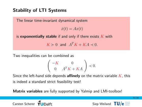
Stability of LTI Systems
47/54
Carsten Scherer Siep Weiland
The linear time-invariant dynamical system
x(t) = Ax(t)
is exponentially stable if and only if there exists K with
K � 0 and AT K + KA ≺ 0.
Two inequalities can be combined as(−K 0
0 AT K + KA
)≺ 0.
Since the left-hand side depends affinely on the matrix variable K, this
is indeed a standard strict feasibility test!
Matrix variables are fully supported by Yalmip and LMI-toolbox!
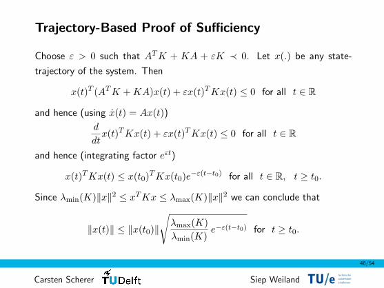
Trajectory-Based Proof of Sufficiency
48/54
Carsten Scherer Siep Weiland
Choose ε > 0 such that AT K + KA + εK ≺ 0. Let x(.) be any state-
trajectory of the system. Then
x(t)T (AT K + KA)x(t) + εx(t)T Kx(t) ≤ 0 for all t ∈ R
and hence (using x(t) = Ax(t))d
dtx(t)T Kx(t) + εx(t)T Kx(t) ≤ 0 for all t ∈ R
and hence (integrating factor eεt)
x(t)T Kx(t) ≤ x(t0)T Kx(t0)e−ε(t−t0) for all t ∈ R, t ≥ t0.
Since λmin(K)‖x‖2 ≤ xT Kx ≤ λmax(K)‖x‖2 we can conclude that
‖x(t)‖ ≤ ‖x(t0)‖
√λmax(K)λmin(K)
e−ε(t−t0) for t ≥ t0.

Algebraic Proof
49/54
Carsten Scherer Siep Weiland
Sufficiency. Let λ ∈ λ(A). Choose a complex eigenvector x 6= 0 with
Ax = λx. Then the LMI’s imply x∗Kx > 0 and
0 > x∗(AT K + KA)x = λx∗Kx + x∗Kxλ = 2Re(λ)x∗Kx.
This guarantees Re(λ) < 0. Therefore all eigenvalues of A are in C−.
Necessity if A is diagonizable. Suppose all eigenvalues of A are in C−.
Since A is diagonizable there exists a complex nonsingular T with TAT−1 =Λ = diag(λ1, . . . , λn). Since Re(λk) < 0 for k = 1, . . . , n we infer
Λ∗ + Λ ≺ 0 and hence (T ∗)−1AT T ∗ + TAT−1 ≺ 0.
If we left-multiply with T ∗ and right-multiply with T (congruence) we infer
AT (T ∗T ) + (T ∗T )A ≺ 0.
Hence K = T ∗T � 0 satisfies the LMI’s.

Algebraic Proof
50/54
Carsten Scherer Siep Weiland
Necessity if A is not diagonizable. If A is not diagonizable it can be
transformed by similarity into its Jordan form: There exists a nonsingular
T with TAT−1 = Λ + J where Λ is diagonal and J has either ones or zeros
on the first upper diagonal.
For any ε > 0 one can even choose Tε with TεAT−1ε = Λ + εJ . Since Λ has
the eigenvalues of A on its diagonal we still infer Λ∗ + Λ ≺ 0. Therefore it
is possible to fix a sufficiently small ε > 0 with
0 � Λ∗ + Λ + ε(JT + J) = (Λ + εJ)∗ + (Λ + εJ).
As before we can conclude that K = T ∗ε Tε satisfies the LMI’s.
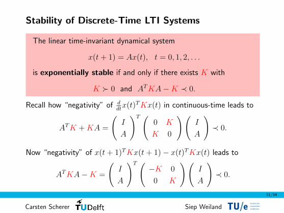
Stability of Discrete-Time LTI Systems
51/54
Carsten Scherer Siep Weiland
The linear time-invariant dynamical system
x(t + 1) = Ax(t), t = 0, 1, 2, . . .
is exponentially stable if and only if there exists K with
K � 0 and AT KA−K ≺ 0.
Recall how “negativity” of ddt
x(t)T Kx(t) in continuous-time leads to
AT K + KA =
(I
A
)T (0 K
K 0
)(I
A
)≺ 0.
Now “negativity” of x(t + 1)T Kx(t + 1)− x(t)T Kx(t) leads to
AT KA−K =
(I
A
)T (−K 0
0 K
)(I
A
)≺ 0.

Outline
51/54
Carsten Scherer Siep Weiland
• From Optimization to Convex Semi-Definite Programming
• Convex Sets and Convex Functions
• Linear Matrix Inequalities (LMIs)
• Truss-Topology Design
• LMIs and Stability
• A First Glimpse at Robustness

A First Glimpse at Robustness
52/54
Carsten Scherer Siep Weiland
With some compact set A ⊂ Rn×n consider the family of LTI systems
x(t) = Ax(t) with A ∈ A.
A is said to be quadratically stable if there exists K such that
K � 0 and AT K + KA ≺ 0 for all A ∈ A.
Why name? V (x) = xT Kx is quadratic Lyapunov function.
Why relevant? Implies that all A ∈ A are Hurwitz.
Even stronger: Implies, for any piece-wise continuous A : R → A,
exponential stability of the time-varying system
x(t) = A(t)x(t).

Computational Verification
53/54
Carsten Scherer Siep Weiland
If A has infinitely many elements, testing quadratic stability amounts
to verifying the feasibility of an infinite number of LMIs.
Key question: How to reduce to a standard LMI problem?
Let A be the convex hull of {A1, . . . , AN}: For each A ∈ A there
exist coefficients λ1 ≥ 0, . . . , λN ≥ 0 with λ1 + · · ·+ λN = 1 such that
A = λ1A1 + · · ·+ λNAN .
If A is the convex hull of {A1, . . . , AN} then A is quadratically
stable iff there exists some K with
K � 0 and ATi K + KAi ≺ 0 for all i = 1, . . . , N.
Proof. Slide 26.

Lessons to be Learnt
54/54
Carsten Scherer Siep Weiland
• Many interesting engineering problems are LMI problems.
• Variables can live in arbitrary vector space.
In control: Variables are typically matrices.
Can involve equation and inequality constraints. Just check whether
cost function and constraints are affine & verify strict feasibility.
• Translation to input for solution algorithm by parser (e.g. Yalmip).
Can choose among many efficient LMI solvers (e.g. Sedumi).
• Main trick in removing nonlinearities so far: Schur Lemma.