Large Margin Linear DiscriminativeVisualization by Matrix Relevance Learning

Michael Biehl∗, Kerstin Bunte†, Frank-Michael Schleif†,Petra Schneider‡ and Thomas Villmann§

∗ University of Groningen, Johann Bernoulli Institute for Mathematics and Computer ScienceP.O. Box 407, NL–9700 AK Groningen, The Netherlands, Email:m.biehl@rug.nl

† University of Bielefeld, Faculty of Technology, CITECD–33594 Bielefeld, Germany

‡ School of Clinical and Experimental Medicine, Centre for Endocrinology and Metabolism CEDAMUniversity of Birmingham, Birmingham B15 2TT, United Kingdom

§ University of Applied Sciences Mittweida, Fakultat fur Mathematik, Physik und InformatikTechnikumplatz 17, D–09648 Mittweida, Germany

Abstract—We suggest and investigate the use of GeneralizedMatrix Relevance Learning (GMLVQ) in the context of discrim-inative visualization. This prototype-based, supervised learningscheme parameterizes an adaptive distance measure in terms ofa matrix of relevance factors. By means of a few benchmarkproblems, we demonstrate that the training process yields lowrank matrices which can be used efficiently for the discriminativevisualization of labeled data. Comparison with well knownstandard methods illustrate the flexibility and discriminativepower of the novel approach. The mathematical analysis ofGMLVQ shows that the corresponding stationarity conditioncan be formulated as an eigenvalue problem with one or severalstrongly dominating eigenvectors. We also study the inclusion ofa penalty term which enforces non-singularity of the relevancematrix and can be used to control the role of higher ordereigenvalues, efficiently.

I. I NTRODUCTION

Given the ever increasing amount of large, high-dimensionaldata sets acquired in a variety scientific disciplines and appli-cation domains, efficient methods for dimension reduction andvisualization play an essential role in modern data processingand analysis.

A multitude of methods for the low-dimensional represen-tation of complex data sets has been proposed in recent years,see for instance [1] for an overview and categorization of themany different approaches. The diversity of methods reflectsthe large number of goals and criteria one can have in mindwith respect to dimension reduction. Indeed, in particularforvisualization, one of the key problems of the field seems tobe the formulation of clear-cut objectives.

A somewhat special case is the discriminative visualizationof labeled data as it occurs in classification problems or othersupervised machine learning frameworks. The classificationaccuracy which can be achieved in the low-dimensional spaceprovides at least one obvious guideline for the evaluation andcomparison of visualizations.

In this contribution we restrict ourselves to methods whichperform an explicit mapping from the original feature spaceto lower dimension [1], [2]. Moreover, we will consider only

linear methods. While limited in power and flexibility, linearmethods continue to be attractive due to their interpretability,low computational costs, and accessibility for mathematicalanalysis.

Probably the most prominent methods that employ linearprojections are the well known Prinicipal Component Analysisfor the unsupervised analysis of data sets and Linear Discrim-inant Analysis in the context of classification problems.

We present a novel, linear approach to the low-dim. repre-sentation and visualization of labeled data which is based on aparticularly powerful and flexible framework for classification.In the recently introduced Generalized Matrix Relevance LVQ[3], a set of prototypes is identified as typical representativesof the classes. At the same time an adaptive distance measureis determined. The latter is parameterized by a matrix whichcorresponds to a linear transformation of feature space. Theoptimization of, both, prototypes and relevance matrix isguided by a margin based cost function. The method displaysan intrinsic tendency to yield a low rank relevance matrix and,hence, its eigenvectors can be employed for discriminativelow-dimensional representation and visualization.

The fact that the approach combines prototype based clas-sification with linear low-dimensional representations makesit a particularly promising technique for interactive tasks.Prototypes serve as typical representatives of the classesandfacilitate good interpretability of the classifier. This isclearlybenefitial in discussions with domain experts. In the context ofvisualization, it offers the possibility tozoom inon regions offeature space which are most representative for the classes.User feedback or data driven, adaptive distance measurescan also be readily employed in the context of interactiveapplications. They can be used, for instance, in the similaritybased retrieval of images from a large data base, see [4]for an example in the medical domain. The combination ofprototype based classification, adaptive similarity measures,and discriminative visualization clearly bears the promise tofacilitate a number of novel techniques for the interactiveanalysis of complex data.

We illustrate the GMLVQ approach to discriminative vi-sualization in terms of a few example data sets, comparingwith the classical approaches of PCA and LDA. Moreover,we present a theoretical analysis which explains the tendencyto low-rank representations in GMLVQ.

II. L INEAR DISCRIMINATIVE VISUALIZATION

We first introduce Generalized Matrix Relevance Learningas a tool for the discriminative low-dimensional representationof labeled data. In addition we review very briefly two classicalstatistical methods: Principal Component Analysis and LinearDiscriminant Analysis.

A. Generalized Matrix Relevance Learning

Similarity based methods play a most important role in,both, unsupervised and supervised machine learning analysisof complex data sets, see [5] for an overview and further refer-ences. In the context of classification problems, Learning Vec-tor Quantization (LVQ), originally suggested by Kohonen [6]–[8], constitutes a particularly intuitive and successful familyof algorithms. In LVQ, classes are represented by prototypeswhich are determined from example data and are defined in theoriginal feature space. Together with a suitable dissimilarity ordistance measure they parameterize the classifier, frequentlyaccording to aNearest Prototypescheme. LVQ schemes areeasy to implement and very flexible. Numerous variations ofthe original scheme have been suggested, aiming at clearermathematical foundation, improved performance, or betterstability and convergence behavior, see e.g. [9]–[13]. Furtherreferences, also reflecting the impressive variety of applicationdomains in which LVQ has been employed successfully, areavailable at [14].

A key issue in LVQ and other similarity based tech-niques is the choice of an appropriate distance measure. Mostfrequently, standard Euclidean or other Minkowski metricsare used without further justification and reflect implicit as-sumptions about, for instance, the presence of approximatelyisotropic clusters

Pre-defined distance measures are, frequently, sensitive torescaling of single features or more general linear transforma-tions of the data. In particular if data is heterogeneous in thesense that features of different nature are combined, usefulnessof Euclidean distance based classification is far from obvious.

An elegant framework has been developed which can cir-cumvent this difficulty to a large extent: In so-called RelevanceLearning schemes, only the functional form of the dissimilarityis fixed, while a set of parameters is determined in the trainingprocess. To our knowledge, this idea was first proposed in [15]in the context of LVQ. Similar ideas have been formulated forother distance based classifiers, see e.g. [16] for an examplein the context of Nearest Neighbor classifiers [17].

A generalized quadratic distance is parameterized by amatrix of relevances in Matrix Relevance Learning which issummarized in the following.

1) The adaptive distance measure:Matrix Relevance LVQ employs a distance measure given bythe quadratic form

d(~y, ~z) = (~y − ~z)⊤ Λ (~y − ~z) for ~y, ~z ∈ RN . (1)

It is required to fulfill the basic conditionsd(~y, ~y) = 0 andd(~y, ~z) = d(~z, ~y) ≥ 0 for all ~y, ~z with ~y 6= ~z. These areconveniently satisfied by assuming the parameterizationΛ =ΩΩ⊤, i.e.

d(~y, ~z) = (~y − ~z)⊤ ΩΩ⊤ (~y − ~z) =[

Ω⊤ (~y − ~z)]2

(2)

Hence,Ω⊤ defines a linear mapping of data and prototypes toa space in which standard Euclidean distance is applied.

In the frame of this contribution we only consider aglobalmetric which is parameterized by a single matrixΛ for allprototypes. Extensions to locally defined distance measures,i.e. local-linear projections, are discussed in [3], [18].

Note that for a meaningful classification and for the LVQtraining it is sufficient to assume thatΛ is positive semi-definite; the transformation need not be invertible and couldeven be represented by a rectangular matrixΩ⊤ [18]. Herewe consider unrestrictedN ×N -matricesΩ without imposingsymmetry or other constraints on its structure. In this case, theelements ofΩ can be varied independently. For instance, thederivative of the distance measure with respect to an arbitraryelement ofΩ is

∂d(~y, ~z)

∂Ωkm

= 2(yk−zk)[

Ω⊤(~y−~z)]

m(3)

or in matrix notation:

∂d(~y, ~z)

∂Ω= = 2 (~y − ~z) (~y − ~z)⊤ Ω. (4)

This derivative is the basis of the matrix adaptation schemeconsidered in the following.

2) Cost function based training:A particularly attractive and successful variant of LVQ, termedGeneralizedLVQ (GLVQ) was introduced by Sato and Ya-mado [10], [11]. Given a set of training examples

~ξν , σνPν=1 where~ξν ∈ RN andσν ∈ 1, 2, . . . , nc

(5)for annc-class problem inN dimensions, training is based onthe cost function

E =1

P

P∑

ν=1

e(~ξν) with e(~ξ) =d(~wJ , ~ξ)− d(~wK , ~ξ)

d(~wJ , ~ξ) + d(~wK , ~ξ)(6)

Here, the indexJ identifies the closest prototype which carriesthe correct labelsJ = σ, the so-calledcorrect winnerwithd(~wJ , ~ξ) = minkd(~wk, ~ξ)|sk = σ. Correspondingly, thewrong winner~wK is the prototype with the smallest distanced(~wi, ~x) among all ~wi representing a different classsi 6= σ.Frequently, an additional sigmoidal functionΦ(e) is applied[10]. While its inclusion would be straightforward, we restrictthe discussion to the simplifying caseΦ(x) = x, in thefollowing.

Note thate(~ξ) in Eq. (6) is negative if the feature vectoris classified correctly. Moreover,−e(~ξ) quantifies the marginof the classification and minimizingE can be interpreted aslarge marginbased training of the LVQ system [10], [19].Matrix relevance learning is incorporated into the frameworkof GLVQ by inserting the distance measure (2) with adaptiveparametersΩ into the cost function (6), see [3].

The popularstochasticgradient descent [20], [21] approxi-mates the gradient∇E by the contribution∇e(~ξν) whereν isselected randomly from1, 2 . . . P in each step. This variantis frequently used in practice as an alternative tobatchgradientdescent where the sum over allν is performed [20].

Given a particular example~ξν , the update of prototypes isrestricted to thewinners ~wJ and ~wK :

~wL ← ~wL − ηw

∂e(~ξν)

∂ ~wL

for L = J,K (7)

see [3] for details and the full form.Updates of the matrixΩ are based on single example

contributions

∂e(~ξν)

∂Ω=

2 dνK

[dνJ + dν

K ]2

∂dνJ

∂Ω−

2 dνJ

[dνJ + dν

K ]2

∂dνK

∂Ω(8)

wheredνL = d(~wL, ~ξν), with derivatives as in Eq. (4).

In the stochastic gradient descent procedure the matrixupdate reads

Ω← Ω− η∂e(~ξν)

∂Ω. (9)

As demonstrated in Sec. III and shown analytically inSec. IV, the GMLVQ approach displays a strong tendencyto yield singular matricesΛ [3], [18] of very low rank.This effect is advantageous in view of potential over-fittingdue to a large number of adaptive parameters. However, therestriction to a single or very few relevant directions canlead to numerical instabilities and might result in inferiorclassification performance if the distance measure becomestoo simple[3], [22]. In order to control this behavior a penaltyterm of the form−µ ln det ΩΩ⊤/2 can be introduced, whichis controlled by a Lagrange parameterµ > 0 and prohibitssingularity ofΛ. The corresponding gradient term [23]

µ

2

∂ ln det ΩΩ⊤

∂Ω= µΩ−T (10)

with the shorthandΩ−T =(

Ω−1)⊤

, is added to the matrixupdate, yielding

Ω← Ω− η∂e(~ξν)

∂Ω+ η µΩ−T (11)

in stochastic descent. Note that the extension to rectangular(N ×M)-matricesΩ (M < N ) is also possible [18], [22]:ReplacingΩ−1 in Eq. (11) by the Moore-Penrose pseudoin-verse [23] enforces rank(Λ) = M.

In the example applications of GMLVQ presented in thefollowing section, protoytpes were initialized close to therespective class-conditional means, with small random devia-tions in order to avoid coinciding vectors~wk. Elements of the

initial Ω were drawn independently from a uniform distributionU(−1,+1) with subsequent normalization

∑

ij Ω2ij = 1.

3) Linear projection of the data set:As discussed above, the adaptive matrixΩ can be interpretedas to define a linear projection for the intrinsic representationof data and prototypes.

Given a particular matrixΛ, the correspondingΩ is notuniquely defined by Eq. (2). Distance measure and classifi-cation performance are, for instance, invariant under rotationsor reflections in feature space andΛ = ΩΩ⊤ can have manysolutions. The actual matrixΩ obtained in the GMVLQ train-ing process will depend on initialization and the randomizedsequence of examples, for instance.

Expressing the symmetricΛ in terms of its eigenvectorsλi

and eigenvectors suggests the canonical representation

Λ =N

∑

i=1

λi ~ui ~u⊤i = ΩΩ⊤ with (12)

Ω =[

√

λ1~u1,√

λ2~u2, . . . ,√

λN~uN

]

,

in which the rows ofΩ⊤ are proportional to the eigenvectorsof Λ. For a low dimensional representation of the data set,the leading eigenvectors ofΛ can be employed, i.e. thosecorresponding to the largest eigenvalues. The fact that thema-trix parameterizes a discriminative distance measure, togetherwith the observation that GMVLQ yields low rank relevancematricesΛ, supports the idea of using this scheme for thevisualization of labeled data sets in classification.

B. Linear Discriminant Analysis

We consider Linear Discriminant Analysis (LDA) in the for-mulation introduced by Fisher [20], [24]–[26]. An alternativeapproach to LDA is based on Bayes decision theory [25]–[27]and is very similar in spirit. For simplicity we will refer toFisher’s discriminant as LDA, in accordance with imprecisebut widespread terminology. Our summary of LDA follows toa large extent the presentation in [20].

Given a data set representingnc classes, cf. Eq. (5), LDAdetermines an(N × [nc − 1])-dim. matrix Γ which defines(nc − 1) linear projections of the data. It is determined as tomaximize an objective function of the form

J(Γ) = Tr[

(

ΓCwΓ⊤)−1 (

ΓCbΓ⊤

)

]

. (13)

Here, Cw and CB are the so-calledwithin-class and thebetween-classcovariance matrix, respectively:

Cw =

nc∑

s=1

P∑

ν=1

δs,σν (~ξν − ~ms)(~ξν − ~ms)

⊤ (14)

Cb =

nc∑

s=1

P∑

ν=1

δs,σν ( ~ms − ~m) ( ~ms − ~m)⊤

with the Kronecker symbolδij =1 if i=j andδij =0 else. Thetotal mean~m and the class-conditional means~ms are directly

−5

0

5

−10

0

10

1

1.5

2

2.5

3

3.5

x

original data

y

z

0 1 2 3 4−1

−0.5

0

0.5

1GMLVQ

−4 −2 0 2 4−1

0

1LDA

−10 −5 0 5 10−1

0

1PCA

Fig. 1. Projection of the three-dim. artificial two-class data set describedin the text, class 1 (2) is represented by grey (black) symbols, respectively.From left to right: original data, projection on the leadingeigenvector ofΛin GMLVQ, projection on the first principal component (upper right) andprojection by LDA (lower right).

estimated from the given data:

~m =1

P

P∑

ν=1

~ξν , and ~ms =

∑

s

∑

ν δσν ,s~ξν

∑

s δσν ,s

. (15)

Assuming that the within-class covariance matrix is invertible,one can show that the rows of the optimalΓ correspond to theleading(nc−1) eigenvectors ofC−1

w Cb. These can be directlydetermined from the given data set and, thus, LDA does notrequire an iterative optimization process.

Note that the between-class covariance matrixCb is of rank(nc−1) [20]. Hence, LDA as described above yields a linearmapping to an(nc−1)-dimensional space. For the purposeof visualization, only the leading eigenvectors ofC−1

w Sb areemployed. Note that for two-class problems, LDA reduces tothe identification of a single direction~γ which maximizes theratio of within class and between class scatter in terms of theprojections~ξν · ~γ [20].

For the results presented in the next section, we have usedthe implementation of Fisher LDA as it is available in van derMaaten’s Toolbox for Dimensionality Reduction [28].

C. Principal Component Analysis

For completeness we also present results obtained by Prin-cipal Component Analysis (PCA) [1], [20], [26]. PCA isarguably the most frequently used projection based techniquefor the exploration and representation of multi-dimensionaldata sets. Several criteria can be employed as a starting pointfor deriving PCA, see [1], [20], [26] for examples.

Given a data set of the form (5), PCA determines theeigenvalues and orthonormal eigenvectors of the covariancematrix

C =

P∑

ν=1

(

~ξν − ~m)(

~ξν − ~m)⊤

. (16)

with the total mean~m given in Eq. (15). The matrixCcan also be written asC = Cw + Cb, cf. Eq. (14). How-ever, unsupervised PCA does not take class membershipsinto account at all. Efficient methods for the calculation ofthe eigenvalue spectrum can be employed in practice. It is,however, very instructive to inspect iterative procedureswhich

−2 0 2−4

−3

−2

−1

0

1

2

3

4PCA

−5 0 5

−10

−5

0

5

10

LDA

−2 −1 0 1 2

−2

−1

0

1

2

GMLVQ

Fig. 2. Two-dimensional visualization of theIris data set as obtained by,from left to right, PCA, LDA, and GMLVQ; see the text for details.

relate to Hebbian learning in the context of neural networks[29], [30].

Conveniently, eigenvectors are ordered according to themagnitude of the corresponding eigenvalues. For a normalizedeigenvector~wi of C with eigenvalueci we have

ci = ~w⊤i C ~wi =

P∑

ν=1

(

~w⊤i

~ξν − ~w⊤i ~m

)2

.

Hence, the eigenvectors mark characteristic directions withvarianceci. The intuitive assumption that a large variance sig-nals high information content of the particular projectioncanbe supported by information theoretic arguments concerningthe optimal reconstruction of original vectors from the linearprojections [1], [20], [26]. For the purpose of two-dimensionalvisualization of data sets in the following section, only the twoleading eigenvectors were employed.

III. C OMPARISON OF METHODS AND ILLUSTRATIVE

EXAMPLES

GMLVQ with 1 prototype per class and LDA are, at aglance, very similar in spirit. Clearly, for well separated, nearlyisotropic classes represented by single prototypes in theircenters one would not expect dramatic differences. However,GLMVQ prototypes are not restricted to positions in the classconditional means which can be advantageous when clustersoverlap. More importantly, a different cost function is opti-mized which appears to be less sensitive to the specific clustergeometry in many cases. In practical applications superiorclassification performance has been found for GMLVQ, evenif two classes are represented by single prototypes, see [31]for a recent example in the biomedical context.

LDA is obviously restricted to data sets which are, at leastapproximately, separable by single linear decision boundaries.LVQ approaches can implement more complex piecewise lin-ear decision boundaries by using several prototypes, reflectingthe cluster geometries and potential multi-modal structures ofthe classes. In combination with relevance matrix training,LVQ retains this flexibility but at the same time bears thepotential to provide a discriminative linear projection ofthedata.

A first obvious example illustrates this flexibility in termsofan artificial toy data set with two classes inN = 3 dimensions,

displayed in Fig. 1 (left panel). Obviously, the data is notlinearly separable. Nevertheless, LDA identifies a well-defineddirection which maximizes the criterion given in Eq. (13). Dueto the elongation of clusters along they-axis in R

3 and thelarge distance of the two class 1 clusters along thez-axis, thedirection of smallest within class variance corresponds tothex-axis. The largest separation of projected class-conditionalmeans would obviously be obtained along thez-axis. In theactual setting, the former dominates the outcome of LDA. Ityields a direction which almost coincides with thex-axis. Aslight deviation prevents the prototypes from coinciding inthe projection. PCA identifies the direction of largest overallvariance, i.e. they-axis in the example setting.

A GMLVQ analysis with an appropriate set of3 prototypes,cf. Fig. 1 (center panel), achieves good classification and adiscriminative one-dimensional visualization at the sametime.Furthermore, its outcome is to a large extent robust withrespect to the precise configuration of the clusters.

A classical illustrative example was already considered byFisher [24]: the well-knownIris data set. It is available fromthe UCI repository [32], for instance. In this simple data set,four features represent properties of 50 individual Iris flowerswhich are to be assigned to one of three different species.

Here we applied az-score transformation before processingthe data by means of PCA, LDA, and GMLVQ. Hence, thedata sets visualized in Figs. 2 and 3 correspond to fourfeatures normalized to zero mean and unit variance. Applyingunsupervised PCA (left panel) shows already that one of theclasses, represented by black symbols, is well separated fromthe other two Iris species which overlap in the two-dim.projection. Although PCA is unsupervised by definition, theobtained visualization happens to be discriminative to a certainextent: A Nearest Neighbor (NN) classification according toEuclidean distance in the two-dim. space misclassifies12% ofthe feature vectors.

For the three class problem, LDA naturally achieves a two-dim. representation, as outlined in Sec. II-B. It results inthevisualization shown in the center panel of Fig. 2. The LDAclassifier achieves an overall misclassification rate of2% onthe data set. NN-classification in the LDA-projected two-dim.space yields3.3% error rate, reflecting that its discriminatingpower is superior compared with unsupervised PCA.

We employed the GMLVQ approach with constant learningratesηw = 0.25 and η = 1.25 · 10−3 in Eq. (7) and (8),respectively. Plain GMLVQ without panelty term achieves anoverall Nearest-Prototype error rate of2%. The rightmostpanel in Fig. 2 displays the visualization according to thetwo leading eigenvectors of the relevance matrixΛ. Thecorresponding Euclidean NN-classification error is also foundto be2%, reflecting the discriminative power of the projection.

The influence of adding a penalty term, Eq. (10), is illus-trated in Fig. 3. The upper left panel corresponds toµ = 0,i.e. original GMLVQ, note the different scaling of axes incomparison with Fig. 2 (right panel). In this case, the firsteigenvalue ofΛ is approximately1 and the resulting projectionis close to one-dimensional, see Fig. 3 (lower row). The

−5 0 5−1

−0.5

0

0.5

1µ=0

−5 0 5−0.8

−0.6

−0.4

−0.2

0

0.2

0.4

0.6µ=0.01

−5 0 5−0.8

−0.6

−0.4

−0.2

0

0.2

0.4

0.6µ=0.1

1 2 3 40

0.2

0.4

0.6

0.8

1

1 2 3 40

0.2

0.4

0.6

0.8

1

1 2 3 40

0.2

0.4

0.6

0.8

1

Fig. 3. Influence of the penalty term (10) in GMLVQ on the visualization ofthe Iris data set. Upper panels: The projection of data and protoytpes (blacksymbols) on the first and second eigenvector of the resulting matrix Λ isdisplayed for, from left to right,µ = 0, µ = 0.01 and µ = 0.1. Lowerpanel: the corresponding eigenvalue spectra of the stationary Λ for the threeconsidered values ofµ.

presence of a penalty term,µ > 0, enforces non-singularΛand higher order eigenvalues increase withµ. At the same timethe scatter of the data along the second eigendirection ofΛbecomes more pronounced. It is interesting to note that, here,the GMLVQ Nearest-Prototype accuracy deteriorates when thepenalty is introduced. While forµ = 0.01 the effect is notyet noticeable, we observe an increased error rate of4% forµ = 0.1. Apparently, optimizing the margin based originalcost function (6) is consistent with achieving low error ratesin this data set.

The Landsatdatabase provides another popular benchmarkavailable at the UCI repository [32]. It consists of6435 featurevectors inR

36, containing spectral intensities of pixels in3×3neighborhoods taken from a satellite image. The classificationconcerns the central pixel in each patch, which is to beassigned to one of 6 classes (red soil, cotton crop, grey soil,damp grey soil, soil with vegetation stubble, very damp greysoil), see [32] for details.

Figure 4 (upper panels) displays the two dimensional visu-alization of the data set as obtained by PCA and LDA. In theprojection restricted to the two leading eigendirections,a Eu-clidean NN-classification scheme achieves overall misclassifi-cation rates of22.4% in the case of PCA and27.9% for LDA.It appears counterintuitive that unsupervised PCA shouldoutperform the supervised LDA with respect to this measure.However, one has to take into account that LDA provides adiscriminative scheme innc−1 = 5 dimensions which is notoptimized with respect to the concept of NN-classification.Inaddition, the restriction to two leading eigendirections limitsthe discriminative power, obviously. Indeed, the unrestrictedLDA system misclassifies only15.2% of the data.

We also display the outcome of GMLVQ training withk = 1 prototype per class andk = 3 prototypes per class,respectively, in Fig. 4 (lower panels). Without the penaltyterm, Eq. (10), the corresponding NN error rates are27.0%

(k = 1) and 18.9% (k = 3), respectively. Visual inspectionalso confirms that better discrimination is achieved with moreprototypes. Of course, the GMLVQ system is also not op-timized with respect to the NN-performance. Indeed, errorrates corresponding to Nearest Prototype classification aresignificantly lower: we obtain16.3% for k = 1 and 15.4%for k = 3 prototypes per class, respectively.

Finally, Fig. 5 exemplifies the influence of the penaltyterm on the GMLVQ system withk = 3 prototypes perclass. The corresponding eigenvalue spectra are displayedinthe rightmost panels. While the leading eigenvalues clearlydominate, the penalty term assigns a certain weight to alleigendirections andΛ remains non-singular.

On the one hand we note that, as higher order directions arecontributing more strongly, the NN-classification in two di-mensions deteriorates slightly: we obtain error rates of20.2%for µ = 0.01 and23.3% with µ = 0.1. On the other hand weobserve that the prototype-distance-based classificationerrorvaries only slightly with the penalty: we obtain error ratesof14.8% for µ = 0.01 and15.2% with µ = 0.1, respectively.

The experiments presented here illustrate the tendency ofGMLVQ to yield low rank relevance matrices. The resultssupport the idea that this classification scheme can be em-ployed for meaningful visualization of labeled data sets. Itis flexible enough to implement complex piecewise lineardecision boundaries in high-dimensional multi-class problems,yet it provides discriminative low-dimensional projections ofthe data, at the same time.

IV. STATIONARITY OF MATRIX RELEVANCE LEARNING

The attractive properties of GMLVQ, as illustrated in theprevious section, can be understood theoretically from thegeneric form of the matrix update, details are presented ina technical report [33]. On average over the random selectionof an example~ξν , the stochastic descent update, Eq. (9), canbe written as

Ω← [I − η G] Ω (17)

with the shorthand~xL = (~ξ − ~wL). Here, the matrixG isgiven as a sum over all example data:

G =1

P

P∑

ν=1

M∑

m,n=1

φJ(~ξν , ~wm)φK(~ξν , ~wn) (18)

×

[

dνm

(dνm + dν

n)2~xν

m ~xν⊤m −

dνn

(dνm + dν

n)2~xν

n ~xν⊤n

]

.

wheredνm = d(~ξν , ~wm). In the sum over pairs of prototypes,

the indicator functionsφJ = 0, 1 singles out the closest correctprototype ~wJ with sJ = σ, while φK = 0, 1 identifies thewrong winner ~wK with sK 6= σ. Obviously, Eq. (17) can beinterpreted as a batch gradient descent step, which coincideswith the averaged stochastic update.

It is important to realize that the matrixG in Eq. (17) doeschange with the LVQ update, in general. Even if prototypespositions are fixed, the assignment of the data to thewinnersas well as the corresponding distances vary withΩ. The

−5 0 5

−5

0

5

10

15

PCA

class1

class2

class3

class4

class5

class6

−15 −10 −5 0 5−6

−4

−2

0

2

4

6

8

LDA

−2 0 2 4 6−2

−1.5

−1

−0.5

0

0.5

1

1.5

2

2.5

GMLVQ, k=1, µ=0

−2 0 2 4 6−4

−2

0

2

4

6

GMLVQ, k=3, µ=0

Fig. 4. Two-dimensional visualizations of thelandsatdata set as described inthe text. Representaion in terms of the two-dim. projections obtained by PCA(upper left panel), LDA (upper right), GMLVQ with one prototype per class(lower left), and with three prototypes per class (lower right). For the sake ofclarity, only 300 randomly selected examples from each class are displayed.Stars mark the projections of GMLVQ protytpes, in addition.

following considerations are based on the assumption thatin the converging system, i.e. after many training steps,Gis reproduced under the update (17). This self-consistencyargument implies that the set of prototypes as well as theassignment of input vectors to the~wk does not change anymoreas Ω is updated. We also have to assume that the individualdistances converge smoothly asΩ approaches its stationarystate. The potential existence of pathological data sets andconfigurations which might violate these assumptions will beprovided in a forthcoming publication.

We would like to emphasize thatG does not have the formof a modified covariance matrixsince it incorporates labelinformation: Examples are weighted with positive or negativesign. Hence,G is not even positive (semi-) definite, in general.Furthermore, the matrix is given as a sum over all prototypes~wk which contribute terms∝ (~ξ − ~wk)(~ξ − ~wk)⊤.

To begin with, we assume that an orderingρ1 < ρ2 ≤ρ3 . . . ≤ ρN of the eigenvalues ofG exists with a uniquesmallest eigenvalueρ1. We exploit the fact that the set ofeigenvectors forms an orthonormal basis~vj

Nj=1 of IRN . The

influence of degeneracies is discussed below.An unnormalized update of the form (17) would be domi-

nated by the largest eigenvalue and corresponding eigenvectorof the matrix[I − η G]. For sufficiently smallη this eigenvalueis (1 − ηρ1) > 0. However, the naive iteration of Eq. (17)without normalization would yield either divergent behavior

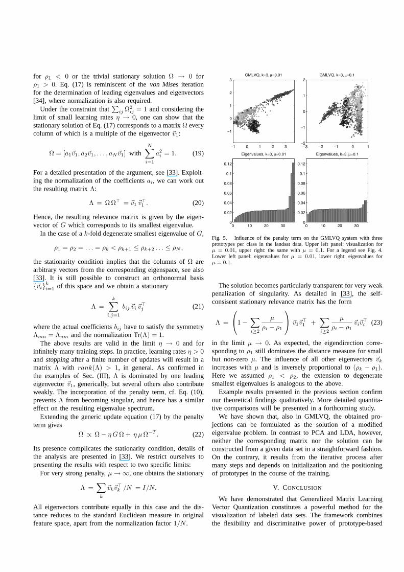
for ρ1 < 0 or the trivial stationary solutionΩ → 0 forρ1 > 0. Eq. (17) is reminiscent of thevon Mises iterationfor the determination of leading eigenvalues and eigenvectors[34], where normalization is also required.

Under the constraint that∑

ij Ω2ij = 1 and considering the

limit of small learning ratesη → 0, one can show that thestationary solution of Eq. (17) corresponds to a matrixΩ everycolumn of which is a multiple of the eigenvector~v1:

Ω = [a1~v1, a2~v1, . . . , aN~v1] withN

∑

i=1

a2i = 1. (19)

For a detailed presentation of the argument, see [33]. Exploit-ing the normalization of the coefficientsai, we can work outthe resulting matrixΛ:

Λ = ΩΩ⊤ = ~v1 ~v⊤1 . (20)

Hence, the resulting relevance matrix is given by the eigen-vector ofG which corresponds to its smallest eigenvalue.

In the case of ak-fold degenerate smallest eigenvalue ofG,

ρ1 = ρ2 = . . . = ρk < ρk+1 ≤ ρk+2 . . . ≤ ρN ,

the stationarity condition implies that the columns ofΩ arearbitrary vectors from the corresponding eigenspace, see also[33]. It is still possible to construct an orthonormal basis~vi

k

i=1of this space and we obtain a stationary

Λ =k

∑

i,j=1

bij ~vi ~v⊤j (21)

where the actual coefficientsbij have to satisfy the symmetryΛmn = Λnm and the normalization Tr(Λ) = 1.

The above results are valid in the limitη → 0 and forinfinitely many training steps. In practice, learning ratesη > 0and stoppingafter a finite number of updates will result in amatrix Λ with rank(Λ) > 1, in general. As confirmed inthe examples of Sec. (III),Λ is dominated by one leadingeigenvector~v1, generically, but several others also contributeweakly. The incorporation of the penalty term, cf. Eq. (10),preventsΛ from becoming singular, and hence has a similareffect on the resulting eigenvalue spectrum.

Extending the generic update equation (17) by the penaltyterm gives

Ω ∝ Ω− η GΩ + η µΩ−T . (22)

Its presence complicates the stationarity condition, details ofthe analysis are presented in [33]. We restrict ourselves topresenting the results with respect to two specific limits:

For very strong penalty,µ→∞, one obtains the stationary

Λ =∑

k

~vk~v⊤k /N = I/N.

All eigenvectors contribute equally in this case and the dis-tance reduces to the standard Euclidean measure in originalfeature space, apart from the normalization factor1/N .

−1 0 1 2 3

−1

0

1

2

3

GMLVQ, k=3, µ=0.01

−3 −2 −1 0 1−2

−1

0

1

2

GMLVQ, k=3, µ=0.1

0 10 20 300

0.02

0.04

0.06

0.08

0.1

0.12

Eigenvalues, k=3, µ=0.01

0 10 20 300

0.02

0.04

0.06

0.08

0.1

0.12

Eigenvalues, k=3, µ=0.1

Fig. 5. Influence of the penalty term on the GMLVQ system with threeprototypes per class in the landsat data. Upper left panel: visualization forµ = 0.01, upper right: the same withµ = 0.1. For a legend see Fig. 4.Lower left panel: eigenvalues forµ = 0.01, lower right: eigenvalues forµ = 0.1.

The solution becomes particularly transparent for very weakpenalization of singularity. As detailed in [33], the self-consisent stationary relevance matrix has the form

Λ =

1−∑

i≥2

µ

ρi − ρ1

~v1~v⊤1 +

∑

i≥2

µ

ρi − ρ1

~vi~v⊤i (23)

in the limit µ → 0. As expected, the eigendirection corre-sponding toρ1 still dominates the distance measure for smallbut non-zeroµ. The influence of all other eigenvectors~vk

increases withµ and is inversely proportional to(ρk − ρ1).Here we assumedρ1 < ρ2, the extension to degeneratesmallest eigenvalues is analogous to the above.

Example results presented in the previous section confirmour theoretical findings qualitatively. More detailed quantita-tive comparisons will be presented in a forthcoming study.

We have shown that, also in GMLVQ, the obtained pro-jections can be formulated as the solution of a modifiedeigenvalue problem. In contrast to PCA and LDA, however,neither the corresponding matrix nor the solution can beconstructed from a given data set in a straightforward fashion.On the contrary, it results from the iterative process aftermany steps and depends on initialization and the positioningof prototypes in the course of the training.

V. CONCLUSION

We have demonstrated that Generalized Matrix LearningVector Quantization constitutes a powerful method for thevisualization of labeled data sets. The framework combinesthe flexibility and discriminative power of prototype-based

classification with the conceptually simple but versatile low-dimensional representation of feature vectors by means of lin-ear projection. Comparison with classical methods of similarcomplexity like LDA and PCA illustrate the usefulness andflexibility of the appraoch.

Furthermore, we have presented an analytic treatment ofthe matrix updates close to stationarity. Like for LDA andPCA, the outcome of GMLVQ can be formulated as a modifiedeigenvalue problem. However, its characteristic matrix cannotbe determined in advance from the data; it depends on theactual training dynamics, including the prototype positions.Consequently, the mathematical treatment of stationarityre-quires a self-consistency assumption. We have extended theanalysis to a variant of GMLVQ which introduces a penaltyterm as to enforce non-singularity of the projection. It controlsthe role of higher-order eigenvalues and allows to influenceproperties of the visualization systematically.

Locally linear extensions of the method which combineglobal, low rank projections with class-specific relevancematrices defined in the low-dimensional space are currentlyinvestigated. This modification can enhance discriminativepower significantly, yet retains the conceptual simplicityofthe visualization.

Our findings indicate that GMLVQ is a promising toolfor discriminative visualization. In particular, we expect avariety of interesting applications in the interactive analysisof complex data sets. In the context of similarity basedretrieval, for instance, extensions along the line of the PicSOMapproach [35] appear promising. The adaptation of the distancemeasure based on user-feedback instead of pre-defined labelsconstitutes another promising application of the approach.

REFERENCES

[1] J. Lee and M. Verleysen,Nonlinear dimensionality reduction. Springer,2007.

[2] K. Bunte, M. Biehl, and B. Hammer, “A general framework for di-mensionaliy reducing data visualization mapping,”Neural Computation,2012.

[3] P. Schneider, M. Biehl, and B. Hammer, “Adaptive relevancematricesin Learning Vector Quantization,”Neural Computation, vol. 21, no. 12,pp. 3532–3561, 2009.

[4] K. Bunte, M. Biehl, M. Jonkman, and N. Petkov, “Learning effectivecolor features for content based image retrieval in dermatology,” PatternRecognition, vol. 44, pp. 1892–1902, 2011.

[5] M. Biehl, B. Hammer, M. Verleysen, and T. Villmann, Eds.,Similaritybased clustering - recent developments and biomedical applications, ser.Lecture Notes in Artificial Intelligence. Springer, 2009, vol. 5400.

[6] T. Kohonen, Self-Organizing Maps, 2nd ed. Berlin, Heidelberg:Springer, 1997.

[7] ——, “Learning Vector Quantization for pattern recognition,” HelsinkiUniveristy of Technology, Espoo, Finland, Tech. Rep. TKK-F-A601,1986.

[8] K. Crammer, R. Gilad-Bachrach, A. Navot, and A. Tishby, “Marginanalysis of the LVQ algorithm,” inAdvances in Neural InformationProcessing Systems, vol. 15. MIT Press, Cambridge, MA, 2003, pp.462–469.

[9] T. Kohonen, “Improved versions of Learning Vector Quantization,” inInternational Joint Conference on Neural Networks, vol. 1, 1990, pp.545–550.

[10] A. Sato and K. Yamada, “Generalized Learning Vector Quantization,”in Advances in Neural Information Processing Systems 8. Proceedingsof the 1995 Conference, D. S. Touretzky, M. C. Mozer, and M. E.Hasselmo, Eds. Cambridge, MA, USA: MIT Press, 1996, pp. 423–429.

[11] ——, “An analysis of convergence in Generalized LVQ,” inProceedingsof the International Conference on Artificial Neural Networks, L. Niklas-son, M. Bodeen, and T. Ziemke, Eds. Springer, 1998, pp. 170–176.

[12] S. Seo and K. Obermayer, “Soft Learning Vector Quantization,” NeuralComputation, vol. 15, no. 7, pp. 1589–1604, 2003.

[13] S. Seo, M. Bode, and K. Obermayer, “Soft nearest prototype classifica-tion,” Transactions on Neural Networks, vol. 14, pp. 390–398, 2003.

[14] Neural Networks Research Centre, “Bibliography on theSelf-OrganizingMap (SOM) and Learning Vector Quantization (LVQ),” Helsinki Uni-versity of Technology.

[15] T. Bojer, B. Hammer, D. Schunk, and K. T. von Toschanowitz,“Rel-evance determination in Learning Vector Quantization,” inEuropeanSymposium on Artificial Neural Networks, M. Verleysen, Ed., 2001, pp.271–276.

[16] K. Weinberger, J. Blitzer, and L. Saul, “Distance metriclearning forlarge margin nearest neighbor classification,” inAdvances in NeuralInformation Processing Systems 18, Y. Weiss, B. Scholkopf, and J. Platt,Eds. Cambridge, MA: MIT Press, 2006, pp. 1473–1480.

[17] T. Cover and P. Hart, “Nearest neighbor pattern classification,” Informa-tion Theory, IEEE Transactions on, vol. 13, no. 1, pp. 21–27, 1967.

[18] K. Bunte, P. Schneider, B. Hammer, F.-M. Schleif, T. Villmann, andM. Biehl, “Limited rank matrix learning, discriminative dimensionreduction and visualization,”Neural Networks, vol. 26, pp. 159–173,2012.

[19] B. Hammer and T. Villmann, “Generalized relevance learning vectorquantization,”Neural Networks, vol. 15, no. 8-9, pp. 1059–1068, 2002.

[20] C. M. Bishop,Neural Networks for Pattern Recognition, 1st ed. OxfordUniversity Press, 1995.

[21] C. Darken, J. Chang, J. C. Z, and J. Moody, “Learning rateschedulesfor faster stochastic gradient search,” inNeural Networks for SignalProcessing 2 - Proceedings of the 1992 IEEE Workshop. IEEE Press,1992.

[22] P. Schneider, K. Bunte, H. Stiekema, B. Hammer, T. Villmann,andM. Biehl, “Regularization in matrix relevance learning,”IEEE Transac-tions on Neural Networks, vol. 21, pp. 831–840, 2010.

[23] K. B. Petersen and M. S. Pedersen, “The matrix cookbook,”http://matrixcookbook.com, 2008.

[24] R. Fisher, “The use of multiple measurements in taxonomic problems,”Annals of Eugenics, vol. 7, pp. 179–188, 1936.

[25] K. Fugunaga,Introduction to Statistical Pattern Recognition, 2nd ed.Academic Press, 1990.

[26] R. Duda, P. Hart, and D. Stork,Pattern Classification, 2nd ed. Wiley-Interscience, 2000.

[27] H. Gao and J. Davis, “Why direct LDA is not equivalent to LDA,”Pattern Recognition, vol. 39, pp. 1002–1006, 2006.

[28] L. van der Maaten, “Matlab toolbox for dimensionality reduction,v0.7.2,” http://homepage.tudelft.nl/19j49/, 2010.

[29] E. Oja, “Neural networks, principal components, and subspaces,”Jour-nal of Neural Systems, vol. 1, pp. 61–68, 1989.

[30] T. Sanger, “Optimal unsupervised learning in a single-layer linear feed-forward neural network,”Neural Networks, vol. 2, pp. 459–473, 1989.

[31] W. Arlt, M. Biehl, A. Taylor, S. Hahner, R. Libe, B. Hughes,P. Schneider, D. Smith, H. Stiekema, N. Krone, E. Porfiri, G. Opocher,J. Bertherat, F. Mantero, B. Allolio, M. Terzolo, P. Nightingale,C. Shackleton, X. Bertagna, M. Fassnacht, and P. Stewart, “Urine steroidmetabolomics as a biomarker tool for detecting malignancy in adrenaltumors,” Journal of Clinical Endocrinology & Metabolism, vol. 96, pp.3775–3784, 2011.

[32] D. J. Newman, S. Hettich, C. L. Blake, and C. J.Merz, “UCI repository of machine learning databases,”http://archive.ics.uci.edu/ml/, 1998.

[33] M. Biehl, B. Hammer, F.-M. Schleif, P. Schneider, and T. Villmann, “Sta-tionarity of Relevance Matrix Learning Vector Quantization,” Universityof Leipzig, Machine Learning Reports, Tech. Rep. MLR 01/2009, 2009.

[34] W. Boehm and H. Prautzsch,Numerical Methods. Vieweg, 1993.[35] J. Laakonen, M. Koskela, S. Laakso, and E. Oja, “PicSOM -content-

based image retrieval with self-organizing maps,”Pattern RecognitionLetters, vol. 21, pp. 1199–1207, 2000.