Learning Discriminative Space–Time Action Parts from Weakly Labelled Videos

International Journal of Computer Vision manuscript No.(will be inserted by the editor)

Learning discriminative space-time action parts from weaklylabelled videos

Michael Sapienza · Fabio Cuzzolin · Philip H.S. Torr

Received: date / Accepted: date

Abstract Current state-of-the-art action classification

methods aggregate space-time features globally, from

the entire video clip under consideration. However, the

features extracted may in part be due to irrelevant scene

context, or movements shared amongst multiple action

classes. For example, a waving action may be performed

whilst walking; if other actions also contain the walk-

ing movement, then the walking features should not be

included to help learn a waving movement classifier.

This motivates learning with local discriminative parts,

which characterise each action class.

Exploiting structure in the video should also im-

prove results, just as pictorial structures have proven

highly successful in object recognition. However, whereas

objects have clear boundaries and easily obtainable ground

truth for initialisation, 3D space-time actions are in-

herently ambiguous and expensive to annotate in large

datasets. Thus, it is desirable to adapt pictorial star

models to action datasets without location annotation,

and to more invariant mid-level features such as bag-of-

feature and Fisher vectors, rather than low-level HoG.

For this, we propose local deformable spatial bag-of-

features (LDSBOF) in which local discriminative re-

gions are split into a fixed grid of parts that are allowed

to deform at test-time.

M. SapienzaOxford Brookes Vision GroupOxford Brookes UniversityOxford, UK.E-mail: [email protected]

F. CuzzolinPresent address: of F. AuthorE-mail: [email protected]

P. H.S TorrPresent address: of F. AuthorE-mail: [email protected]

We demonstrate that by using general video sub-

volumes, and by augmenting mid-level features with

deformable structures, we are able to achieve state-of-

the-art classification performance, whilst being able to

localise space-time actions even in the most challenging

datasets.

Keywords Action classification · localisation ·multiple instance learning · pictorial structures ·space-time videos

1 Introduction

Human action recognition from video is an increasingly

prominent research area in computer vision, with far-

reaching applications. On the web, the recognition ofhuman actions will soon allow the organisation, search,

description, and retrieval of information from the mas-

sive amounts of video data uploaded each day (Kuehne

et al, 2011). In every day life, human action recogni-

tion has the potential to provide a natural way to com-

municate with robots, and novel ways to interact with

computer games and virtual environments.

In addition to being subject to the usual nuisance

factors such as variations in illumination, viewpoint,

background and part occlusions, human actions inher-

ently possess a high degree of geometric and topological

variability (Bronstein et al, 2009). Various human mo-

tions can carry the exact same meaning. For example,

a jumping motion may vary in height, frequency and

style, yet still be the same action. Action recognition

systems need then to generalise over actions in the same

class, while discriminating between actions of different

classes (Poppe, 2010).

Despite these difficulties, significant progress has been

made in learning and recognising human actions from

2 Michael Sapienza et al.

videos (Poppe, 2010; Weinland et al, 2011). Whereas

early action recognition datasets included videos with

single, staged human actions against simple, static back-

grounds (Schuldt et al, 2004; Blank et al, 2005), more

recently challenging uncontrolled movie data (Laptev

et al, 2008) and amateur video clips available on the In-

ternet (Liu et al, 2009; Kuehne et al, 2011) have been

used to evaluate action recognition algorithms. These

datasets contain human actions with large variations in

appearance, style, viewpoint, background clutter and

camera motion, common in the real world.

Current space-time human action classification meth-

ods (Jiang et al, 2012; Vig et al, 2012; Kliper-Gross

et al, 2012; Wang et al, 2011) derive an action’s rep-

resentation from an entire video clip, even though this

representation may contain motion and scene patterns

pertaining to multiple action classes. For instance, in

the state-of-the-art bag-of-feature (BoF) approach (Wang

et al, 2009), dense space-time features are aggregated

globally into a single histogram representation per video.

This histogram is generated from features extracted

from the whole video and so includes visual word counts

originating from irrelevant scene background (Fig. 1a -

b), or from motion patterns shared amongst multiple

action classes. For example the action classes ‘trampo-

line jumping’ and ‘volleyball spiking’ from the YouTube

dataset (Liu et al, 2009) both involve jumping actions,

and have a similar scene context, as shown in Fig. 1c-

d. Therefore in order to discriminate between them, it

is desirable to automatically select those video parts

which tell them apart, such as the presence of a moving

ball, multiple actors and other action-specific charac-

teristics.

This motivates a framework in which action mod-

els are derived from smaller portions of the video vol-

ume, subvolumes, which are used as learning primitives

rather than the entire space-time video. Thus, we pro-

pose to cast action classification in a weakly labelled

framework, in which only the global label of each video

clip is known, and not the label of each individual video

subvolume. In this way, action models may be derived

from automatically selected video parts which are most

discriminative of the action. An example illustrating

the result of localising discriminative action parts with

models learnt from weak annotation is shown in Fig. 2.

In addition to discriminative local action models, we

propose to incorporate deformable structure by learn-

ing a pictorial star model for each action class. In the

absence of ground truth location annotation, we use the

automatically selected video regions to learn a ‘root’ ac-

tion model. Action part models are subsequently learnt

from the root location after dividing it into a fixed grid

(a) boxing (b) running

(c) trampoline jumping (d) volleyball spiking

Fig. 1 The disadvantages of using global information to rep-resent action clips. Firstly, global histograms contain irrele-vant background information as can be seen in the (a) Boxingand (b) Running action videos of the KTH dataset (Schuldtet al, 2004). Secondly, the histograms may contain frequencycounts from similar motions occurring in different actionclasses, such as the (c) trampoline jumping and (d) volley-ball spiking actions in the YouTube dataset (Liu et al, 2009).In this paper, we propose a framework in which action modelscan be derived from local video subvolumes which are morediscriminative of the action. Thus important differences suchas the moving ball, the presence of multiple people and otheraction-specific characteristics may be captured.

of regions, which are allowed to deform at test-time.

This extends spatial-BoF models (Parizi et al, 2012) to

incorporate deformable structure. The result of testing

a 3-part handwaving model is shown in Fig. 3.

The crux of this paper deals with the problem of

automatically generating action models from weakly la-

belled observations. By extending global mid-level rep-

resentations to general video subvolumes and deformable

part-models, we are able to both improve classification

results, as compared to the global baseline, and capture

location information.

2 Previous Work

State-of-the-art results in action classification from chal-

lenging human data have recently been achieved by us-

ing a bag-of-features approach (Jiang et al, 2012; Vig

et al, 2012; Kliper-Gross et al, 2012; Wang et al, 2011).

Typically, in a first stage, local spatio-temporal struc-

ture and motion features are extracted from video clips

and quantised to create a visual vocabulary. A query

video clip is then represented using the frequency of

Learning discriminative space-time action parts from weakly labelled videos 3

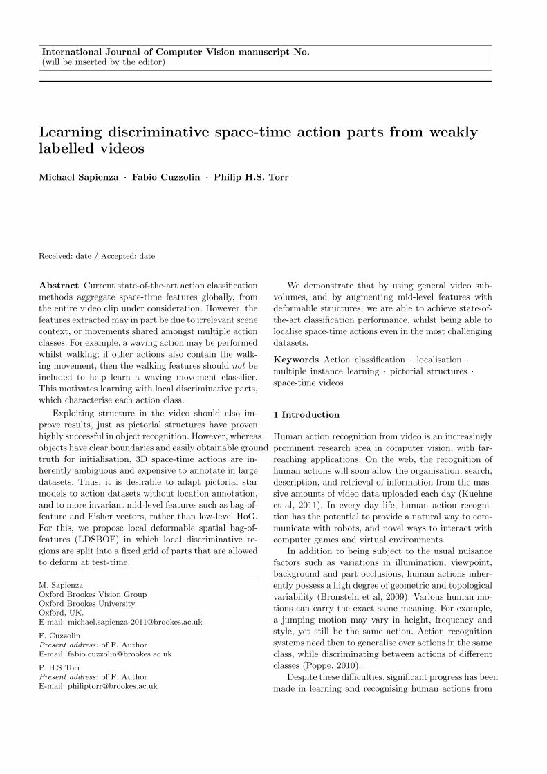
Fig. 2 A handwaving video sequence taken from the KTHdataset (Schuldt et al, 2004) plotted in space and time. No-tice that in this particular video, the handwaving motion isrepeated continuously and the camera zoom is varying withtime. Overlaid on the video is a dense handwaving-action lo-cation map, where each pixel is associated with a score indi-cating its class-specific saliency. This dense map was gener-ated by aggregating detection scores from general subvolumes‘types’, and is displayed sparsely for clarity, where the colour,from blue to red, and sparsity of the plotted points indicatethe action class membership strength. Since the scene contextof the KTH dataset is not discriminative for this particularaction, only the movement in the upper body of the actor isdetected as salient (best viewed in colour).

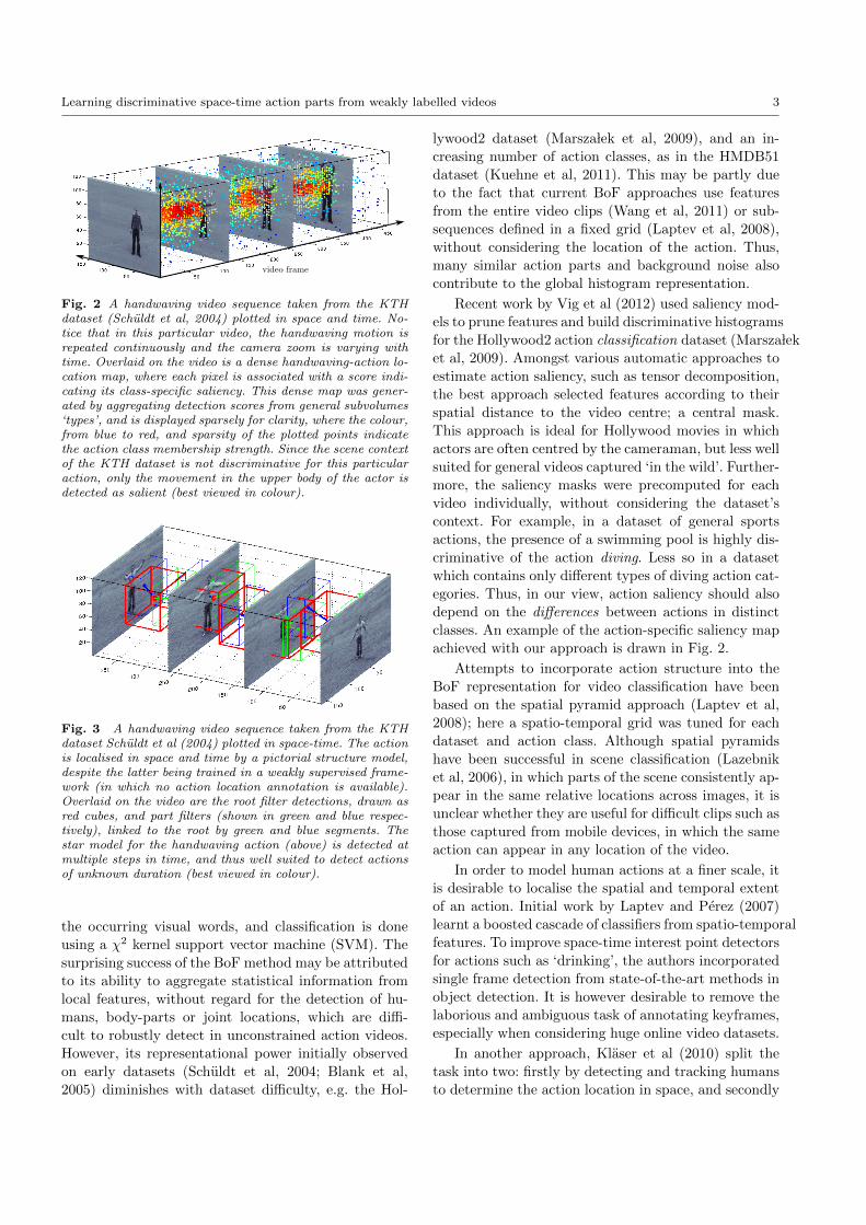
Fig. 3 A handwaving video sequence taken from the KTHdataset Schuldt et al (2004) plotted in space-time. The actionis localised in space and time by a pictorial structure model,despite the latter being trained in a weakly supervised frame-work (in which no action location annotation is available).Overlaid on the video are the root filter detections, drawn asred cubes, and part filters (shown in green and blue respec-tively), linked to the root by green and blue segments. Thestar model for the handwaving action (above) is detected atmultiple steps in time, and thus well suited to detect actionsof unknown duration (best viewed in colour).

the occurring visual words, and classification is done

using a χ2 kernel support vector machine (SVM). The

surprising success of the BoF method may be attributed

to its ability to aggregate statistical information from

local features, without regard for the detection of hu-

mans, body-parts or joint locations, which are diffi-

cult to robustly detect in unconstrained action videos.

However, its representational power initially observed

on early datasets (Schuldt et al, 2004; Blank et al,

2005) diminishes with dataset difficulty, e.g. the Hol-

lywood2 dataset (Marsza lek et al, 2009), and an in-

creasing number of action classes, as in the HMDB51

dataset (Kuehne et al, 2011). This may be partly due

to the fact that current BoF approaches use features

from the entire video clips (Wang et al, 2011) or sub-

sequences defined in a fixed grid (Laptev et al, 2008),

without considering the location of the action. Thus,

many similar action parts and background noise also

contribute to the global histogram representation.

Recent work by Vig et al (2012) used saliency mod-

els to prune features and build discriminative histograms

for the Hollywood2 action classification dataset (Marsza lek

et al, 2009). Amongst various automatic approaches to

estimate action saliency, such as tensor decomposition,

the best approach selected features according to their

spatial distance to the video centre; a central mask.

This approach is ideal for Hollywood movies in which

actors are often centred by the cameraman, but less well

suited for general videos captured ‘in the wild’. Further-

more, the saliency masks were precomputed for each

video individually, without considering the dataset’s

context. For example, in a dataset of general sports

actions, the presence of a swimming pool is highly dis-

criminative of the action diving. Less so in a dataset

which contains only different types of diving action cat-

egories. Thus, in our view, action saliency should also

depend on the differences between actions in distinct

classes. An example of the action-specific saliency map

achieved with our approach is drawn in Fig. 2.

Attempts to incorporate action structure into the

BoF representation for video classification have been

based on the spatial pyramid approach (Laptev et al,

2008); here a spatio-temporal grid was tuned for each

dataset and action class. Although spatial pyramids

have been successful in scene classification (Lazebnik

et al, 2006), in which parts of the scene consistently ap-

pear in the same relative locations across images, it is

unclear whether they are useful for difficult clips such as

those captured from mobile devices, in which the same

action can appear in any location of the video.

In order to model human actions at a finer scale, it

is desirable to localise the spatial and temporal extent

of an action. Initial work by Laptev and Perez (2007)

learnt a boosted cascade of classifiers from spatio-temporal

features. To improve space-time interest point detectors

for actions such as ‘drinking’, the authors incorporated

single frame detection from state-of-the-art methods in

object detection. It is however desirable to remove the

laborious and ambiguous task of annotating keyframes,

especially when considering huge online video datasets.

In another approach, Klaser et al (2010) split the

task into two: firstly by detecting and tracking humans

to determine the action location in space, and secondly


by using a space-time descriptor and sliding window

classifier to temporally locate two actions (phoning,

standing up). In a similar spirit, our goal is to localise

actions in space and time, rather than time alone (Duchenne

et al, 2009; Gaidon et al, 2011). However, instead of

resorting to detecting humans in every frame using a

sliding window approach (Klaser et al, 2010), we lo-

calise actions directly in space-time, either by aggregat-

ing detection scores as a measure of saliency (Fig. 2), or

by visualising the 3D bounding box detection windows

(Fig. 3).

To introduce temporal structure into the BoF frame-

work, Gaidon et al (2011) introduced Actom Sequence

Models, based on a non-parametric generative model.

In video event detection, Ke et al (2010) used a search

strategy in which oversegmented space-time video re-

gions were matched to manually constructed volumet-

ric action templates. Inspired by the pictorial structures

framework (Fischler and Elschlager, 1973), which has

been successful at modelling object part deformations

(Felzenszwalb et al, 2010), Ke et al (2010) split their

action templates into deformable parts making them

more robust to spatial and temporal action variabil-

ity. Despite these efforts, the action localisation tech-

niques described (Laptev and Perez, 2007; Klaser et al,

2010; Ke et al, 2010) require manual labelling of the

spatial and/or temporal (Gaidon et al, 2011) extent of

the actions/parts in a training set. In contrast, we pro-

pose to learn discriminative models automatically from

weakly labelled observations, without human location

annotation. Moreover, unlike previous work (Gilbert

et al, 2009; Liu et al, 2009), we select discriminative

action instances represented by local mid-level features

(Boureau et al, 2010) such as BoF and Fisher vectors,

and not the low-level space-time features themselves

(e.g. HoG, HoF).

We propose to split up each video clip into overlap-

ping subvolumes of cubic/cuboidial structure, and to

represent each video clip by a set of mid-level vectors,

each associated with a single subvolume. Since in action

clip classification only the class of each action clip as a

whole is known, and not the class labels of individual

subvolumes, this problem is inherently weakly-labelled.

We therefore cast video subvolumes and associated rep-

resentations as instances in a discriminative multiple

instance learning (MIL) framework.

Some insight into MIL comes from its use in the

context of face detection (Viola et al, 2005). Despite

the availability of ground truth bounding box annota-

tion, the improvement in detection results when com-

pared to those of a fully supervised framework sug-

gested that there existed a more discriminative set of

ground truth bounding boxes than those labelled by hu-

man observers. The difficulty in manual labelling arises

from the inherent ambiguity in labelling objects or ac-

tions (bounding box scale, position) and judging, for

each image/video, whether the context is important for

that particular example or not. A similar MIL approach

was employed by Felzenszwalb et al (2010) for object

detection in which possible object part bounding box

locations were cast as latent variables. This allowed the

self-adjustment of the positive ground truth data, bet-

ter aligning the learnt object filters during training.

In order to additionally incorporate action struc-

ture, we follow the work of Felzenszwalb et al (2010),

and enrich local mid-level representations using a sim-

ple star-structured part-based model, defined by a ‘root’

filter, a set of ‘parts’, and a structure model. The ob-

jects considered by Felzenszwalb et al (2010) have a

clear boundary which is annotated by ground truth

bounding boxes. During training, the ground truth boxes

were critical for finding a good initialisation of the ob-

ject model, and also constrained the plausible position

of object parts. Furthermore, the aspect ratio of the

bounding box was indicative of the viewpoint is was

imaged from, and was used to split each object class

into a mixture of models (Felzenszwalb et al, 2010). In

contrast, for action classification datasets such as the

ones used in this work, the spatial location, the tem-

poral duration and the number of action instances are

not known beforehand. Therefore we propose an alter-

native approach to learning ‘root’ and ‘part’ filters in

a 2-step process, employing mid-level representations,

rather than low-level HoG features (Felzenszwalb et al,

2010; Tian et al, 2013) to capture the richness of each

action class.

Firstly, in the absence of ground truth annotation,

we train ‘root’ filters in a discriminative (MIL) frame-

work (Andrews et al, 2003). In a second step we allow

the learning of part-specific models by splitting the root

filter into a grid of fixed regions. The learning of parts

directly split from the root is motivated by the distri-

bution of features within the root subvolume, which is

likely to be similar across different instances detected by

the same root filter. Thus, one can split the root action

subvolume in two and learn separate models for each

part, as done in spatial pyramids (Lazebnik et al, 2006;

Parizi et al, 2012). In contrast to the rigid global grid

regions of spatial pyramids (Lazebnik et al, 2006) or

spatial-BoF (Parizi et al, 2012), our rigid template used

during training is local, not global, and is allowed to de-

form at test-time to better capture the action warping

in space and time, as illustrated in Fig. 4(a)&(b).

At test time, human action classification is achieved

by the recognition of action instances in the query video,

after devising a sensible mapping from instance scores


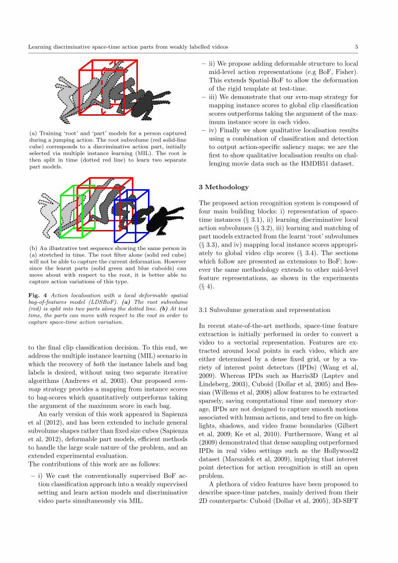
(a) Training ‘root’ and ‘part’ models for a person capturedduring a jumping action. The root subvolume (red solid-linecube) corresponds to a discriminative action part, initiallyselected via multiple instance learning (MIL). The root isthen split in time (dotted red line) to learn two separatepart models.

(b) An illustrative test sequence showing the same person in(a) stretched in time. The root filter alone (solid red cube)will not be able to capture the current deformation. Howeversince the learnt parts (solid green and blue cuboids) canmove about with respect to the root, it is better able tocapture action variations of this type.

Fig. 4 Action localisation with a local deformable spatialbag-of-features model (LDSBoF). (a) The root subvolume(red) is split into two parts along the dotted line. (b) At testtime, the parts can move with respect to the root in order tocapture space-time action variation.

to the final clip classification decision. To this end, we

address the multiple instance learning (MIL) scenario in

which the recovery of both the instance labels and bag

labels is desired, without using two separate iterative

algorithms (Andrews et al, 2003). Our proposed svm-

map strategy provides a mapping from instance scores

to bag-scores which quantitatively outperforms taking

the argument of the maximum score in each bag.

An early version of this work appeared in Sapienza

et al (2012), and has been extended to include general

subvolume shapes rather than fixed size cubes (Sapienza

et al, 2012), deformable part models, efficient methods

to handle the large scale nature of the problem, and an

extended experimental evaluation.

The contributions of this work are as follows:

– i) We cast the conventionally supervised BoF ac-

tion classification approach into a weakly supervised

setting and learn action models and discriminative

video parts simultaneously via MIL.

– ii) We propose adding deformable structure to local

mid-level action representations (e.g BoF, Fisher).

This extends Spatial-BoF to allow the deformation

of the rigid template at test-time.

– iii) We demonstrate that our svm-map strategy for

mapping instance scores to global clip classification

scores outperforms taking the argument of the max-

imum instance score in each video.

– iv) Finally we show qualitative localisation results

using a combination of classification and detection

to output action-specific saliency maps; we are the

first to show qualitative localisation results on chal-

lenging movie data such as the HMDB51 dataset.

3 Methodology

The proposed action recognition system is composed of

four main building blocks: i) representation of space-

time instances (§ 3.1), ii) learning discriminative local

action subvolumes (§ 3.2), iii) learning and matching of

part models extracted from the learnt ‘root’ subvolumes

(§ 3.3), and iv) mapping local instance scores appropri-

ately to global video clip scores (§ 3.4). The sections

which follow are presented as extensions to BoF; how-

ever the same methodology extends to other mid-level

feature representations, as shown in the experiments

(§ 4).

3.1 Subvolume generation and representation

In recent state-of-the-art methods, space-time feature

extraction is initially performed in order to convert a

video to a vectorial representation. Features are ex-

tracted around local points in each video, which are

either determined by a dense fixed grid, or by a va-

riety of interest point detectors (IPDs) (Wang et al,

2009). Whereas IPDs such as Harris3D (Laptev and

Lindeberg, 2003), Cuboid (Dollar et al, 2005) and Hes-

sian (Willems et al, 2008) allow features to be extracted

sparsely, saving computational time and memory stor-

age, IPDs are not designed to capture smooth motions

associated with human actions, and tend to fire on high-

lights, shadows, and video frame boundaries (Gilbert

et al, 2009; Ke et al, 2010). Furthermore, Wang et al

(2009) demonstrated that dense sampling outperformed

IPDs in real video settings such as the Hollywood2

dataset (Marsza lek et al, 2009), implying that interest

point detection for action recognition is still an open

problem.

A plethora of video features have been proposed to

describe space-time patches, mainly derived from their

2D counterparts: Cuboid (Dollar et al, 2005), 3D-SIFT


(Scovanner et al, 2007), HoG-HoF (Laptev et al, 2008),

Local Trinary Patterns (Yeffet and Wolf, 2009) HOG3D

(Klaser et al, 2008), extended SURF (Willems et al,

2008), and C2-shape features (Jhuang et al, 2007). More

recently Wang et al (2011) proposed Dense Trajectory

features which, when combined with the standard BoF

pipeline (Wang et al, 2009), outperformed the recent

Learned Hierarchical Invariant features (Le et al, 2011;

Vig et al, 2012). Therefore, even though this framework

is independent from the choice of features, we use the

Dense Trajectory features (Wang et al, 2011) to de-

scribe space-time video blocks.

Dense Trajectory features are formed by the se-

quence of displacement vectors in an optical flow field,

together with the HoG-HoF descriptor (Laptev et al,

2008) and the motion boundary histogram (MBH) de-

scriptor (Dalal et al, 2006) computed over a local neigh-

bourhood along the trajectory. The MBH descriptor

represents the gradient of the optical flow, and captures

changes in the optical flow field, suppressing constant

motions (e.g. camera panning) and capturing salient

movements. Thus, Dense Trajectories capture a tra-

jectory’s shape, appearance, and motion information.

These features are extracted densely from each video at

multiple spatial scales, and a pruning stage eliminates

static trajectories such as those found on homogeneous

backgrounds, or spurious trajectories which may have

drifted (Wang et al, 2011).

In order to aggregate local space-time features, we

use the BoF approach, proven to be very successful at

classifying human actions in realistic settings, and also

compare them to Fisher vectors, proven to be highly

successful in image classification (Jegou et al, 2011).

However instead of aggregating the features over the en-

tire video volume (Wang et al, 2011), or within a fixed

grid (Laptev et al, 2008), we aggregate features within

local subvolumes of various cuboidial sizes scanned densely

within the video, (Fig. 5). In practice, there is a huge

number of possible subvolume shapes at different scales

in videos of varying resolution and length in time. There-

fore we have chosen a representative set of 12 subvolume

‘types’, as a compromise between localisation and clas-

sification accuracy and the computational complexity

associated with considering more subvolume types. The

subvolumes range from small cubes to larger cuboids

which span the whole range of the video in space and

time, as illustrated in Fig. 5.

Note that by considering only the subvolume which

corresponds to the maximum size, the representation

of each video reduces to that of the standard global

pipeline (Wang et al, 2011). The exact parameter set-

tings for subvolume generation are detailed with the

experimental evaluation in Section 4.

Fig. 5 Local space-time subvolume ‘types’ are drawn in twovideos of varying length at random locations. These subvol-umes represent the regions in which local features are aggre-gated to form a vectorial representation.

In contrast to object detection, in which the bound-

aries of an object are well defined in space, the ambigu-

ity and inherent variability of actions means that not all

actions are well captured by bounding boxes. Therefore

we propose to represent discriminative action locations

by an action-specific saliency map. At test-time, each

subvolume will be associated with a vector of scores de-

noting the response of each action class in that region.

Since in our framework, we also map the individual in-

stance scores to a global video clip classification score

(§ 3.4), the vector of scores associated with each sub-

volume can be reduced to that of the predicted video

action class. It is therefore possible to build an action-

specific saliency map by aggregating the predicted de-

tection scores from all instances within the space-time

video (Fig. 2).

3.2 MIL-BoF action models

In this work, when using BoF, we define an instance

to be an individual histogram obtained by aggregating

the Dense Trajectory features within a local subvol-

ume, and a bag is defined as a set of instances originat-

ing from a single space-time video. Since we perform

multi-class classification with a 1-vs-rest approach, we

present the following methodology as a binary classifi-

cation problem.


(a) Global space-time volume (b) Bag of general local subvolumes

Fig. 6 Instead of defining an action as a space-time pattern in an entire video clip (a), an action is defined as a collection ofspace-time action parts contained in general subvolumes shapes of cube/cuboidial shape (b). One ground-truth action label isassigned to the entire space-time video or ‘bag’, while the labels of each action subvolume or ‘instance’ are initially unknown.Multiple instance learning is used to learn which instances are particularly discriminative of the action (solid-line cubes), andwhich are not (dotted-line cubes).

In action classification datasets, each video clip is

assigned to a single action class label. By decomposing

each video into multiple instances, now only the class

of the originating video is known and not those of the

individual instances. This makes the classification task

weakly labelled, where it is known that positive exam-

ples of the action exist within the video clip, but their

exact location is unknown. If the label of the bag is

positive, then it is assumed that one or more instances

in the bag will also be positive. If the bag has a nega-

tive label, then all the instances in the bag must retain

a negative label. The task here is to learn the class

membership of each instance, and an action model to

represent each class, as illustrated in Fig. 6.

The learning task may be cast in a max-margin

multiple instance learning framework, of which the pat-

tern/instance margin formulation (Andrews et al, 2003)

is best suited for space-time action localisation. Let the

training set D = (〈X1, Y1〉, ..., 〈Xn, Yn〉) consist of a

set of bags Xi = {xi1, ...,ximi} of different length mi,

with corresponding ground truth labels Yi ∈ {−1,+1}.Each instance xij ∈ R represents the jth BoF model

in the ith bag, and has an associated latent class label

yij ∈ {−1,+1} which is initially unknown for the posi-

tive bags (Yi = +1). The class label for each bag Yi is

positive if there exists at least one positive instance in

the bag, that is, Yi = maxj{yij}. Therefore the task of

the mi-MIL is to recover the latent class variable yij of

every instance in the positive bags, and to simultane-

ously learn an SVM instance model 〈w, b〉 to represent

each action class.

The max-margin mi-SVM learning problem results

in a semi-convex optimisation problem, for which An-

drews et al (2003) proposed a heuristic approach. In mi-

SVM, each instance label is unobserved, and we max-

imise the usual soft-margin jointly over hidden variables

and discriminant function:

minyij

minw,b,ξ

1

2‖w‖2 + C

∑ij

ξij , (1)

subject to : yij(wTxij + b) ≥ 1− ξij , ∀i, j

yij ∈ {−1,+1}, ξij ≥ 0,

and∑j∈i

(1 + yij)/2 ≥ 1 s.t. Yi = +1,

yij = −1 ∀j∈i s.t. Yi = −1,

where w is the normal to the separating hyperplane, b

is the offset, and ξij are slack variables for each instance

xij .

The heuristic algorithm proposed by Andrews et al

(2003) to solve the resulting mixed integer problem is

laid out in Algorithm 1. Consider training a classi-

fier for a walking class action from the bags of train-

ing instances in a video dataset. Initially all the in-

stances are assumed to have the class label of their par-

ent bag/video (STEP 1). Next, a walking action model

estimate 〈w, b〉 is found using the imputed labels yij(STEP 2), and scores

fij = wTxij + b, (2)

for each instance in the bag are estimated with the cur-

rent model (STEP 3). Whilst the negative labels remain

strictly negative, the positive labels may retain their

current label, or switch to a negative label (STEP 4). If,

however, all instances in a positive bag become nega-

tive, then the least negative instance in the bag is set to


Algorithm 1 Heuristic algorithm proposed by (An-

drews et al, 2003) for solving mi-SVM.

STEP 1. Assign positive labels to instances in positive bags:yij = Yi for j ∈ irepeat

STEP 2. Compute SVM solution 〈w, b〉 for instanceswith estimated labels yij .STEP 3. Compute scores fij = wTxij + b for all xij inpositive bags.STEP 4. Set yij = sgn(fij) for all j ∈ i, Yi = 1.for all positive bags Xi do

if∑

j∈i(1 + yij)/2 == 0 then

STEP 5. Find j∗ = argmaxj∈i

fij , set y∗ij = +1

end ifend for

until class labels do not changeOutput w, b

have a positive label (STEP 5), thus ensuring that there

exists at least one positive example in each positive bag.

Now consider walking video instances whose feature

distribution is similar to those originating from bags in

distinct action classes. The video instances originating

from the walking videos will have a positive label, whilst

those from the other action classes will have a negative

label (assuming a 1-vs-all classification approach). This

corresponds to a situation where points in the high di-

mensional instance space are near to each other. Thus,

when these positive walking instances are reclassified in

a future iteration, it is likely that their class label will

switch to negative. As the class labels are updated in

an iterative process, eventually only the discriminative

instances in each positive bag are retained as positive.

The resulting SVM model 〈w0, b0〉 represents the root

filter in our space-time BoF star model.

3.3 Local Deformable SBoF models (LDSBoF)

In order to learn space-time part models, we first se-

lect the best scoring root subvolumes learnt via Algo-

rithm 1. The selection is performed by first pruning

overlapping detections with non-maximum suppression

in three dimensions, and then picking the top scor-

ing 5%. Subvolumes are considered to be overlapping

if their intersection over the union is greater that 20%.

This has the effect of generating a more diverse sam-

ple of high scoring root subvolumes to learn the part

models from.

The part models are generated by splitting the root

subvolumes using a fixed grid, as would be done in spa-

tial bag-of-features (SBoF) (Parizi et al, 2012). For our

experiments we split the root into p = 2 equal-sized

blocks along the time dimension, as shown in Fig. 4(a),

and recalculate BoF vectors for each part. We found

that with our current dense low-level feature sampling

density (§ 4.3), further subdividing the root to gener-

ate more parts creates subvolumes which are too small

to aggregate meaningful statistics. Finally, part models

〈wk, bk〉, k = {1...p}, are individually learnt in terms

of a standard linear SVM. The grid structure of SBoF

removes the need to learn a structure model for each

action class, which simplifies training, especially since

no exact or approximate location annotation is avail-

able to constrain the part positions (Felzenszwalb et al,

2010).

In the following, an action is defined in terms of a

collection of space-time action-parts in a pictorial struc-

ture model (Fischler and Elschlager, 1973; Felzenszwalb

and Huttenlocher, 2005; Ke et al, 2010), as illustrated in

Fig. 4(b). Following the notation of Felzenszwalb and

Huttenlocher (2005), let an action be represented by

an undirected graph G = (V,E), where V = {v1, ...vp}collects the p parts of the action, and (vk, vl) ∈ E rep-

resents a connection between part vk and vl. An in-

stance of the action’s configuration is defined by a vec-

tor L = (l1, ...lp), where lk ∈ R3 specifies the location of

part vk. The detection space S(x, y, z) is represented by

a feature map H of BoF histograms for each subvolume

at position lk, and there exists for each action part, a

BoF filter wk, which when correlated with a subvolume

in H, gives a score indicating the presence of the action

part vk. Thus, the dot product

wk · φ(H, lk), (3)

measures the correlation between a filter wk and a fea-

ture map H at location lk in the video. Let the dis-

tance between action parts dkl(lk, ll) be a cost function

measuring the degree of deformation of connected parts

from a model. The overall score for an action located

at root position l0 is calculated as:

sij(l0) = maxl1 ,...lp

(p∑k=0

wk · φ(Hi, lk)−p∑k=1

dkl(lk, ll)

),

(4)

which optimises the appearance and configuration of

the action parts simultaneously. The scores defined at

each root location may be used to detect multiple ac-

tions, or mapped to bag scores in order to estimate

the global class label (c.f. section 3.4). Felzenszwalb

et al (2010) describe an efficient method to compute

the best locations of the parts as a function of the root

locations, by using dynamic programming and gener-

alised distance transforms (Felzenszwalb and Hutten-

locher, 2004).


In practice, we do not calculate a root filter response

(4) densely for each pixel, but rather on a subsampled

grid (§ 4.3.1). When processing images (e.g. 2D object

detection) one may pad the empty grid locations with

low scores and subsample the distance transform re-

sponses (Felzenszwalb et al, 2010) with little perfor-

mance loss, since high scores are spread to nearby loca-

tions taking into consideration the deformation costs.

However with video data, the difference in the num-

ber of grid locations for the full and subsampled video

is huge. For example, between an image grid of size

640× 480, and one half its size, there is a difference of

approx 23×104 pixel locations. In a corresponding video

of length 1000 frames (approx. 30 seconds), the differ-

ence in the number of grid locations is 26 × 107. Even

though the efficient distance transform algorithm scales

linearly with the number of possible locations, padding

empty grid locations with low scores becomes computa-

tionally expensive. Therefore we modified the distance

transform algorithm to only compute the lower enve-

lope of the parabolas bounding the solution (Felzen-

szwalb and Huttenlocher, 2004) at the locations defined

by a sparse grid. In this way we achieve the exact same

responses with a significant speedup.

3.4 A learnt mapping from instance to bag labels

So far the focus has been on learning instance-level

models for detection. However in order to make a clas-

sification decision, the video class label as a whole also

needs to be estimated.

The instance margin MIL formulation detailed in

section 3.2 aims at recovering the latent variables of

all instances in each positive bag. When recovering the

optimal labelling yij and the optimal hyperplane 〈w, b〉(1), all the positive and negative instances in a positive

bag are considered. Thus, only the query instance labels

may be predicted:

yij = sgn(wTxij + b). (5)

An alternative MIL approach called the ‘bag margin’

formulation is typically adopted to predict the bag la-

bels. The ‘bag-margin’ approach adopts a similar iter-

ative procedure as the ‘instance margin’ formulation,

but only considers the ‘most positive’ and ‘most neg-

ative’ instance in each bag. Therefore predictions take

the form:

Yi = sgn maxj∈i

(wTxij + b), (6)

where 〈w, b〉 are the model parameters learnt from the

‘bag-margin’ formulation (Andrews et al, 2003).

In order to avoid this iterative procedure for retriev-

ing the bag labels, and to additionally map root scores

obtained with the pictorial structures approach of sec-

tion 3.3, we propose a simple and robust alternative

method in which bag scores are directly estimated from

the instance scores fij (2) or sij (4). One solution is to

use the same max decision rule in (6) with the instance

scores: Yi = sgn maxj∈i(fij). However, the scores from

the max may be incomparable, and are often calibrated

on a validation set to increase performance (Platt, 1999;

Lin et al, 2007). Moreover, better cues may exist to pre-

dict the bag label. Cross-validation can be used to select

a threshold on the number of positive instances in each

bag, or a threshold on the mean instance score in each

bag. The downside is that the number of instances in

each bag may vary significantly between videos, making

values such as the mean instance score between bags in-

comparable. For example, in a long video clip in which

a neatly performed action only occupies a small part,

there would be large scores for instances containing the

action, and low scores elsewhere. Clearly, the mean in-

stance score would be very low, even though there was

a valid action in the clip.

As a more robust solution we propose to construct

a feature vector by combining multiple cues from the

instance scores fij in each bag, including the number

of positive instances, the mean instance scores, and the

maximum instance score in each bag. The feature vector

Fi is constructed as follows:

Fi =[#p, #n,

#p

#n,

1

n

∑j(fij), max

j∈i(fij),min

j∈i(fij)

],

(7)

where #p and #n are the number of positive and nega-

tive instances in each bag respectively. In this way, the

variable number of instance scores in each bag are rep-

resented by a six-dimensional feature vector fij 7→ Fi,and a linear SVM decision boundary, 〈w′, b′〉, is learnt

from the supervised training set D = (〈F1, Y1〉, ...,〈Fn, Yn〉), in this constant dimensional space. Now pre-

dictions take the form:

Yi = sgn(w′TFi + b′). (8)

Apart from mapping multiple instance scores to single

bag scores, this svm-map strategy generates compara-

ble bag scores for various action classes, thus avoiding

any instance score calibration. Moreover, in the follow-

ing experimental section, we demonstrate that our svm-

map strategy outperforms taking the argument of the

maximum instance score in each bag, even after the

scores have been Platt-calibrated.


Fig. 7 A sample of images from the various datasets usedin the experimental evaluation. Whereas early action recog-nition datasets like the KTH (Schuldt et al, 2004) includedvideos with single, staged human actions against homoge-neous backgrounds, more recently challenging uncontrolledmovie data from the Hollywood2 dataset (Marsza lek et al,2009) and amateur video clips available on the Internet seenin the YouTube (Liu et al, 2009) and HMDB51 (Kuehneet al, 2011) datasets are being used to evaluate action recog-nition algorithms. These challenging datasets contain humanactions which exhibit significant variations in appearance,style, viewpoint, background clutter and camera motion, asseen in the real world.

4 Experimental Evaluation & Discussion

In order to validate our action recognition system, we

evaluated its performance on four challenging human

action classification datasets, namely the KTH, YouTube,

Hollywood2 and HMDB51 datasets, sample images of

which are shown in Fig. 7. We give a brief overview of

each dataset (§ 4.1), the experiments (§ 4.2) and their

parameter settings (§ 4.3), followed by an ensuing dis-

cussion of the classification (§ 4.5), timings (§ 4.6) and

localisation (§ 4.7) results.

4.1 Datasets

The KTH dataset (Schuldt et al, 2004) contains 6 ac-

tion classes (walking, jogging, running, boxing, waving,

clapping) each performed by 25 actors, in four scenar-

ios. We split the video samples into training and test

sets as in (Schuldt et al, 2004); however, we considered

each video clip in the dataset to be a single action se-

quence, and did not further slice the video into clean,

smaller action clips. This may show the robustness of

our method to longer video sequences which include

noisy segments in which the actor is not present.

The YouTube dataset (Liu et al, 2009) contains 11

action categories (basketball shooting, biking/ cycling,

diving, golf swinging, horse back riding, soccer juggling,

swinging, tennis swinging, trampoline jumping, volley-

ball spiking and walking with a dog), and presents sev-

eral challenges due to camera motion, object appear-

ance, scale, viewpoint and cluttered backgrounds. The

1600 video sequences were split into 25 groups, and we

followed the author’s evaluation procedure of 25-fold,

leave-one-out cross validation.

The Hollywood2 dataset (Marsza lek et al, 2009) con-

tains 12 action classes : answering phone, driving car,

eating, fighting, getting out of car, hand-shaking, hug-

ging, kissing, running, sitting down, sitting up, and

standing up, collected from 69 different Hollywood movies.

There are a total of 1707 action samples containing re-

alistic, unconstrained human and camera motion. We

divided the dataset into 823 training and 884 testing se-

quences, as done by Marsza lek et al (2009). The videos

for this dataset, each from 5-25 seconds long, were down-

sampled to half their size (Le et al, 2011).

The HMDB dataset (Kuehne et al, 2011) contains

51 action classes, with a total of 6849 video clips col-

lected from movies, the Prelinger archive, YouTube and

Google videos. Each action category contains a mini-

mum of 101 clips. We used the non-stabilised videos

with the same three train-test splits as the authors

(Kuehne et al, 2011).

4.2 Experiments and performance measures

In a first batch of experiments, we employed our local

discriminative part learning (c.f. MIL-BoF, section 3.2)

without adding structure, in order to i) determine its

performance with respect to our global baseline (§ 4.4.4),

ii) assess how the dimensionality of the instance repre-

sentation affected performance, and iii) compare BoF

and Fisher representations. Furthermore, iv) we com-

pared three ways of mapping instance scores to a fi-

nal bag classification score: a) taking the argument of

the maximum value in each bag (max), b) calibrating

the instance scores by fitting a sigmoid function to the

SVM outputs (Platt, 1999; Lin et al, 2007) before tak-

ing the max (max platt), and c) using our proposed

svm-map mapping strategy (c.f. section 3.4). We would

also like to address questions such as: i) What is the rel-

ative difficulty of each dataset? and ii) How important is

feature dimensionality for discriminating between more

classes? The results are presented in Fig. 8 and Table 1,

where one standard deviation from the mean is reported


for those datasets which have more than one train/test

set.

In a second batch of experiments, we employed the

top performing mid-level feature representation and di-

mensionality and extended it with a 3-part pictorial

structure model (c.f section 3.3), to determine the mer-

its of adding local deformable structure to mid-level

action models. The quantitative results of LDSBoF-3

are listed in Table 1.

Previous methods have evaluated action classifica-

tion performance through a single measure, such as the

accuracy or average precision. In our experimental eval-

uation, we used three performance measures for each

dataset, in order to present a more complete picture of

each algorithm’s performance, namely:

– Accuracy (Acc), calculated as the #correctly clas-

sified testing clips /#total testing clips,

– Average precision (AP), which considers the order-

ing in which the results are presented,

– F1-score, which weights recall and precision equally

and is calculated as the ratio:

F1 =2× recall× precision

recall + precision. (9)

4.3 Parameter settings

Dense Trajectory features were computed in video blocks

of size 32 × 32 pixels for 15 frames, with a dense sam-

pling step size of 5 pixels, as set by default (Wang et al,

2011).

4.3.1 Subvolumes

All subvolume types were extracted from a regular grid

with a spacing of 20 pixels in space and time. This

spacing was chosen to balance the higher accuracy ob-

tainable with higher densities, with the computational

and storage cost associated with thousands of high di-

mensional vectors. Results are reported for a general

mixture of subvolume types, as opposed to fixed sized

cuboids (Sapienza et al, 2012), allowing for two scales in

width, two scales in height, and 3 scales in time, where

the largest scale stretches over the whole video. The

smallest subvolume takes a size of 60×60×60 pixels in

a video of resolution 160× 120, and scales accordingly

for videos of higher resolutions. This setup generated a

total of 2×2×3 subvolume types within each space-time

volume, as illustrated in Fig. 5. Typical values for the

number of subvolumes extracted per video ranged from

approximately 300 to 3000, depending on the length of

each video.

4.3.2 BoF

Each Dense Trajectory feature was split into its 5 types

(trajectory 30-D, HOG 96-D, HOF 108-D, MBHx 96-

D, MBHy 96-D), and for each type, a separate K-word

visual vocabulary was built by k-means. In order to

generate the visual vocabulary, a random and balanced

selection of videos from all action classes were sub-

sampled, and 106 features were again sampled at ran-

dom from this pool of features. The k-means algorithm

was initialised 8-times and the configuration with the

lowest error was selected. Lastly, each BoF histogram

was L1 normalised separately for each feature type, and

then jointly. To speed up the histogram generation we

employed a fast kd-tree forest (Muja and Lowe, 2009;

Vedaldi and Fulkerson, 2008) to quantise each Dense

Trajectory feature to its closest cluster centre, deliver-

ing a four times speedup when compared to calculating

the exact Euclidean distance.

4.4 χ2 kernel approximation

The total number of subvolumes in the each dataset

depends on the number and length of the individual

videos. For example with the current settings (§ 4.3.1)

on the Hollywood2 dataset there are approx. 3×106 in-

stances, each a high dimensional histogram, making the

learning problem at hand large-scale. Therefore we used

the approximate homogeneous kernel map by Vedaldi

and Zisserman (2010) instead of the exact χ2 kernel,

which in practice takes a prohibitively long time to

compute due to the large number of instances generated

from each dataset. The feature map is based on additive

kernels (Vedaldi and Zisserman, 2010), and provides an

approximate, finite dimensional linear representation in

closed form. The χ2 kernel map parameters were set to

N=1, and a homogeneity degree of γ=0.5, which gives

a K ×(2N + 1

)dimensional approximated kernel map.

4.4.1 Fisher vectors

Using Fisher vectors has the advantage that top results

may be achieved without using a feature map, and using

only linear-SVM classifiers, which scale much more effi-

ciently with an increasing number of training instances

(Perronnin et al, 2010). Due to the high dimension-

ality of Fisher vectors, each Dense Trajectory feature

type was initially reduced to 24 dimensions using PCA

(Rokhlin et al, 2009). For each feature type, a separate

visual vocabulary was built with K-Gaussians each via

EM. The features used to learn the dictionary were sam-

pled in the exact same manner as for BoF (§ 4.3.2). We


follow Perronnin et al (2010) and applied power nor-

malisation followed by L2 normalisation to each Fisher

vector component separately, before normalising them

jointly.

4.4.2 Fast linear-SVM solver

In order to quickly learn linear SVM models with thou-

sands of high-dimensional vectors, we employed the PE-

GASOS algorithm (Shalev-Shwartz et al, 2011). This

stochastic subgradient descent method for solving SVMs

is well suited for learning linear classifiers with large

data, since the run-time does not directly depend on

the number of instances in the training set. We used

the batch formulation with size k=100, and stopped

the optimisation after 500 iterations if the required tol-

erance (10−3) was not satisfied. Stopping the optimisa-

tion early results in quicker training and helps gener-

alisation by preventing over-fitting. In order to address

class imbalance, we sampled a balanced set of positive

and negative examples without re-weighting the objec-

tive function (Perronnin et al, 2012).

4.4.3 Multiple instance learning

Initially, all the instances in each positive bag were set

to have a positive label. At each iteration, the SVM

solver was initialised with the model parameters 〈w, b〉calculated in the previous iteration (Andrews et al, 2003),

as well as the previous learning iteration number at

which 〈w, b〉 were calculated. Instead of fixing the SVM

regularisation parameters to values known to work well

on the test set, we performed 5-fold cross validation

(Kuehne et al, 2011) on the training set, and automat-

ically select the best performing models based on the

validation set accuracy. Multi-class classification is per-

formed using the one-vs-all approach.

4.4.4 Baseline global algorithm

The baseline approach was set-up by using only the

largest subvolume, the one corresponding to the entire

video clip. This reduces to the pipeline described in

Wang et al (2011), except that in our setup approx-

imate methods are used for histogram building and

model learning.

4.4.5 Local Deformable Spatial BoF

The part model subvolumes were set to half the size

of the resulting learnt root subvolumes, as shown in

Fig 4(a) & Fig 12. We modelled the relative position of

each part with respect to the root node centre of mass

as a Gaussian with diagonal covariance (Ke et al, 2010):

dkl(lk, ll) = βN (lk − ll, skl,∑kl) (10)

where lk − ll represents the distance between part vkand vl, sij is the mean offset and represents the an-

chor points of each part with respect to the root, and∑kl is the diagonal covariance. The parameter β which

adjusts the weighting between appearance and configu-

ration scores is set to 0.01 throughout. The mean offset

is taken automatically from the geometrical configura-

tion resulting from the splitting of the root filter during

training, and is set to the difference between the root’s

and the part’s centres of mass. The covariance of each

Gaussian is set to half the size of the root filter.

4.5 Results and discussion

First we turn to the results presented in Figs 8(a)-

8(d), where for each dataset, the classification accu-

racy of various approaches (see Fig. 8(d)) were plotted

for comparison. For each set of experiments, the mid-

level feature dimensionality was varied by controlling

the K-centroids used to build each visual vocabulary.

The dimensions of KBoF (approximate kernel-mapped

BoF) vectors were calculated as: K (centroids) ×5 (fea-

ture types) ×3 (kernel-map). The dimensions of Fisher

vectors were calculated as: 2 (Fisher w.r.t mean and

variance (Perronnin et al, 2010)) ×K (centroids) ×5

(feature types) ×24 (dimensions per feature type after

PCA).

From the result plots of Fig. 8, a number of inter-

esting observations emerged. First, even with a 16 fold

reduction in K and without a kernel feature mapping,

Fisher vectors outperformed KBoF, both in global and

local representations. It is even quite surprising that

with only 2 clusters per Dense Trajectory feature type,

Fisher vectors achieve over 90% accuracy on the KTH

dataset, a sign of the dataset’s ease. The relative diffi-

culty of each dataset is initially indicated by the chance

level drawn as a grey horizontal line. However this does

not take into consideration the noise in the dataset la-

belling or the choice of train-test splittings. For exam-

ple, the YouTube and Hollywood2 datasets both have

nearly the same chance level, however from the results

plots it is clear that the Hollywood2 dataset is more

challenging.

Notice that the Hollywood2 and HMDB datasets

saw a steady increase in performance with increasing

K; less so for the KTH and YouTube datasets, a sign

that cross-validation over K may improve results on

certain datasets. On the YouTube dataset, also notice


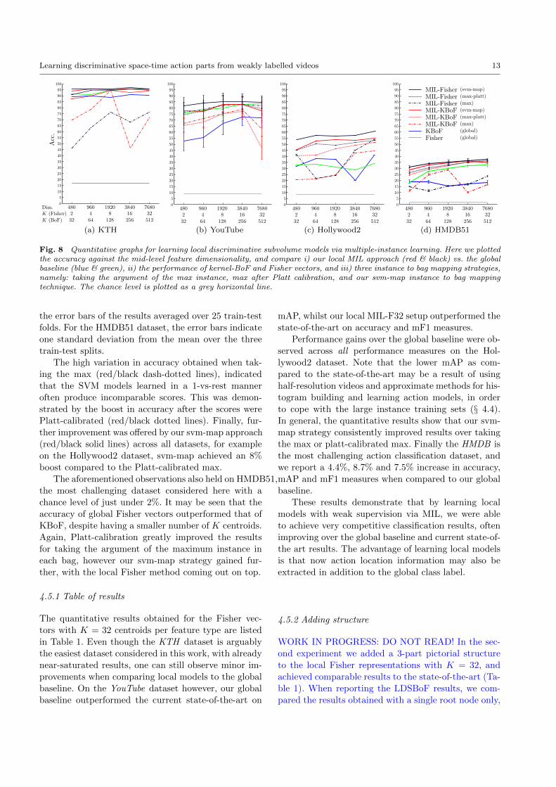
(a) KTH (b) YouTube (c) Hollywood2 (d) HMDB51

Fig. 8 Quantitative graphs for learning local discriminative subvolume models via multiple-instance learning. Here we plottedthe accuracy against the mid-level feature dimensionality, and compare i) our local MIL approach (red & black) vs. the globalbaseline (blue & green), ii) the performance of kernel-BoF and Fisher vectors, and iii) three instance to bag mapping strategies,namely: taking the argument of the max instance, max after Platt calibration, and our svm-map instance to bag mappingtechnique. The chance level is plotted as a grey horizontal line.

the error bars of the results averaged over 25 train-test

folds. For the HMDB51 dataset, the error bars indicate

one standard deviation from the mean over the three

train-test splits.

The high variation in accuracy obtained when tak-

ing the max (red/black dash-dotted lines), indicated

that the SVM models learned in a 1-vs-rest manner

often produce incomparable scores. This was demon-

strated by the boost in accuracy after the scores were

Platt-calibrated (red/black dotted lines). Finally, fur-

ther improvement was offered by our svm-map approach

(red/black solid lines) across all datasets, for example

on the Hollywood2 dataset, svm-map achieved an 8%

boost compared to the Platt-calibrated max.

The aforementioned observations also held on HMDB51,

the most challenging dataset considered here with a

chance level of just under 2%. It may be seen that the

accuracy of global Fisher vectors outperformed that of

KBoF, despite having a smaller number of K centroids.

Again, Platt-calibration greatly improved the results

for taking the argument of the maximum instance in

each bag, however our svm-map strategy gained fur-

ther, with the local Fisher method coming out on top.

4.5.1 Table of results

The quantitative results obtained for the Fisher vec-

tors with K = 32 centroids per feature type are listed

in Table 1. Even though the KTH dataset is arguably

the easiest dataset considered in this work, with already

near-saturated results, one can still observe minor im-

provements when comparing local models to the global

baseline. On the YouTube dataset however, our global

baseline outperformed the current state-of-the-art on

mAP, whilst our local MIL-F32 setup outperformed the

state-of-the-art on accuracy and mF1 measures.

Performance gains over the global baseline were ob-

served across all performance measures on the Hol-

lywood2 dataset. Note that the lower mAP as com-

pared to the state-of-the-art may be a result of using

half-resolution videos and approximate methods for his-

togram building and learning action models, in order

to cope with the large instance training sets (§ 4.4).

In general, the quantitative results show that our svm-

map strategy consistently improved results over taking

the max or platt-calibrated max. Finally the HMDB is

the most challenging action classification dataset, and

we report a 4.4%, 8.7% and 7.5% increase in accuracy,

mAP and mF1 measures when compared to our global

baseline.

These results demonstrate that by learning local

models with weak supervision via MIL, we were able

to achieve very competitive classification results, often

improving over the global baseline and current state-of-

the art results. The advantage of learning local models

is that now action location information may also be

extracted in addition to the global class label.

4.5.2 Adding structure

WORK IN PROGRESS: DO NOT READ! In the sec-

ond experiment we added a 3-part pictorial structure

to the local Fisher representations with K = 32, and

achieved comparable results to the state-of-the-art (Ta-

ble 1). When reporting the LDSBoF results, we com-

pared the results obtained with a single root node only,


Table 1 A table showing the state-of-the-art results, and ourresults using Fisher K-32 for various approaches.

KTH Acc mAP mF1State-of-the-art 96.761 97.021 96.041

Global-F32 95.37 96.81 95.37MIL-F32(max) 95.83 97.43 95.84MIL-F32(max-platt) 95.83 97.43 95.82MIL-F32(svm-map) 96.76 97.88 96.73LDSBoF-3 95.83 96.97 95.84LDSBoF-3(svm-map) 96.76 95.27 96.76

YOUTUBE Acc mAP mF1State-of-the-art 84.202 86.101 77.351

Global-F32 83.64±6.43 87.18±3.58 80.41±7.90

MIL-F32(max) 81.84±6.68 86.53±4.65 78.59±8.31

MIL-F32(max-platt) 79.22±5.88 86.53±4.65 74.35±7.56

MIL-F32(svm-map) 84.52±5.27 86.73±5.43 82.43±6.33

Hollywood2 Acc mAP mF1State-of-the-art 39.631 59.53, 60.04 39.421

Global-F32 33.94 40.42 12.18MIL-F32(max) 53.96 49.25 39.11MIL-F32(max-platt) 52.94 49.25 36.34MIL-F32(svm-map) 60.85 51.72 52.03

HMDB51 Acc mAP mF1State-of-the-art 31.531 40.73 25.411

Global-F32 32.79±1.46 30.98±0.69 30.62±1.19

MIL-F32(max) 23.33±0.66 35.87±0.56 16.68±0.40

MIL-F32(max-platt) 36.19±0.56 35.88±0.56 32.86±0.34

MIL-F32(svm-map) 37.21±0.69 39.69±0.47 38.14±0.76

1Sapienza et al (2012), 2Wang et al (2011), 3Jiang et al(2012), 4Vig et al (2012).

and the results obtained by including the parts and

structure. It can be seen that between the Fisher root

model and the Fisher 3-star model, there is an apprecia-

ble improvement, indicating the value of adding parts

to the model. Comparing the global Fisher and localFisher star methods, its can be seen that despite the

better Fisher star results obtained on the KTH dataset,

lower results were obtained for the Hollywood2 dataset.

This may be due to the appreciable noise in the Hol-

lywood2 and the approximate SVM learning compared

to the exact method for the global approach.

4.6 Computational timings

The experiments were carried out on a machine with 8,

2GHz CPUs and 32GB of RAM. The timings we report

here are for running the method MIL-F32 in the table

of results on the HMDB dataset. Building the visual

vocabulary took 4 CPU hours, whilst the local aggre-

gation of Dense Trajectory features in to fisher vectors

took 13 CPU days. Finally, 5 CPU days were needed for

learning local discriminative subvolumes via MIL. Since

the implementation is non optimised in MATLAB, we

are convinced that the computational timings can be

Fig. 9 Action classification and localisation on the KTHdataset. (a) This boxing video sequence has been correctlyclassified as a boxing action, and has overlaid the boxing ac-tion saliency map to indicate the location of discriminativeaction parts. (b) This time, the action classified is that ofa walking action. In this longer video sequence, the actorwalks in and out of the camera shot, as shown by the densered points over the locations in which the actor was presentin the shot.

cut considerably. Note that the low-level feature extrac-

tion, the local aggregation, and 1-vs-rest classification

are easily parallelised.

4.7 Qualitative localisation

In addition to action clip classification, the learnt local

instance models can also be used for action localisation,

the results of which are discussed in the next sections.

4.7.1 Class-specific saliency

The qualitative saliency maps of Fig. 9 demonstrate the

action location information gained in addition to the

classification label. Recall that each subvolume is asso-

ciated with a vector of scores where each element de-

notes the score for each action category in the dataset.

The saliency map was computed by aggregating the in-

stance scores associated with each subvolume ‘type’ in

each video. However since we also estimated the global

video clip class label, the vector of scores per subvol-

ume can be reduced to that of the predicted class. Thus

in both Fig. 9a & b, the saliency map is specific to

the predicted global action class, and is displayed as a


Fig. 10 Action localisation results on the HMDB51 dataset,the most challenging action classification dataset to date. In(d), a girl is pouring liquid into a glass, and in (e) a personis pushing a car. Notice that the push action does not fireover the person’s moving legs but rather on the contact zonebetween the person and the vehicle. Moreover the saliencymap in (b) is focused on the bow and not on the person’selbow movement.

sparse set of points for clarity, where the colour, from

blue to red, and sparsity of the plotted points indi-

cate the action class membership strength. Moreover,

the saliency map indicates the action location in both

space and time. In both videos of Fig. 9, irrelevant scene

background, common in most of the KTH classes, was

pruned by the MIL during training, and therefore the

learnt action models were able to better detect relevant

action instances. Notice that the saliency map was able

to capture both the consistent motion of the boxing

action in Fig. 9a, as well as the intermittent walking

action of Fig. 9b.

The qualitative localisation results for the HMDB

dataset are shown in Fig. 10 and Fig. 11, where the

saliency maps drawn over the videos are those corre-

sponding to the predicted global action class. Note that

such a saliency map does not represent a general mea-

sure of saliency (Vig et al, 2012), rather it is specific

Fig. 11 Misclassifications in the HMDB dataset. The pre-dicted class is shown first, followed by the ground truth classin brackets. Note that the localisation scores shown are ofthe predicted class. (a) A ‘kick ball’ action that has framesof Britney Spears singing in the middle. (b) A ‘push’ actionwrongly classified as ‘climb’. (c) The fast swinging movementof the ‘baseball’ action was classified as ‘catch’. (d) A hugwas incorrectly classified as punch, and (e) a ‘punch’ wasmisclassified as ‘clap’. (f) In this case the wave action wasmisclassified as walk, even though President Obama was alsowalking. The algorithm was unable to cope with the situationin which two actions occur simultaneously.

to the particular action class being considered. This has

the effect of highlighting discriminative parts of the ac-

tion, for example, in the pushing action of Fig. 10e, the

contact between the hands and vehicle is highlighted,

less so the leg’s motion. Likewise in Fig. 10d the pour-

ing action is highlighted, less so the arm’s motion. The

videos of Fig. 11 show the results obtained when the

clip is incorrectly classified. In this case, higher scores

are located at the borders of the video frame, since the

instance scores for the wrong predicted class are low

over the video parts where the action occurs. In the

HMDB dataset, apart from dealing with a wide range

of action classes, our algorithm has to deal with sig-

nificant nuisance factors in the data, such as frames of

‘Britney Spears’ singing in between a ‘kick ball’ action

(Fig. 11a), and the possibility of multiple actions per

video clip such as the ‘walking’ and ‘waving’ actions in

Fig. 11f. Extending the proposed framework in order

to deal with multiple actions per video is left for future

work.

4.7.2 Bounding box detection with LDSBoF

LDSBoF also predicts the location of discriminative

parts of the action, this time with 3D bounding boxes


Fig. 12 (a) Top, and (b) side views from a test boxing videosequence in the KTH dataset. Plotted are the top 5 best partconfigurations found in the video volume. The simple tree-structured star models are drawn with blue and green links tothe root node.

and a space-time pictorial structure model. This is clearly

seen in Fig. 12, where the top and side views of a box-

ing video sequence from the KTH dataset are plotted

in space-time.

¡WORK IN PROGRESS¿ The space-time plots of

Figs. 13(a)-(f) show qualitative results obtained when

detecting actions with Fisher star models; it can be

seen that the highest scoring detections do indeed cor-

respond to discriminative parts of the action. For ex-

ample in the boxing video of Fig. 13(a), the root and

part nodes are centred on the person’s arms, whilst

in the running video of Fig. 13(f), the detections ap-

pear around the legs of the actor. Thus, our proposed

method it is well suited for other action localisation

datasets (Laptev and Perez, 2007; Klaser et al, 2010;

Gaidon et al, 2011), which we leave for future work.

5 Conclusion

We proposed a novel general framework for action clip

classification and localisation based on the recognition

of local space-time subvolumes. A number of interesting

insights emerged. Our experiments qualitatively demon-

strated that it is possible to localise challenging actions

captured ‘in the wild’, with weak annotation, whilst

achieving state-of-the-art classification results. Since in

our approach the detection primitives were space-time

subvolumes, there was no need to perform spatial and

temporal detection separately (Liu et al, 2009). Rather,

each subvolume was associated with a location in the

video, and a decision score for each action class.

Even though our method is independent of the choice

of mid-level feature representation, we found that Fisher

vectors performed the best when compared to kernel-

mapped BoF histograms. The experimental results on

four major action classification datasets further demon-

strated that our local subvolume approach outperformed

the global baseline on the majority of performance mea-

sures. We expect that by increasing the number of pos-

sible subvolumes and the density at which they are ex-

tracted, we will observe further improvements in clas-

sification and localisation accuracy. Further MIL per-

formance gains may be obtained by multiple random

initialisations, instead of assigning each instance to the

label of their parent bag, although at higher computa-

tional cost. Investigating the importance of each cue in

the svm-map feature vector may also reveal improved

mapping strategies.

¡WORK IN PROGRESS¿ Our LDSBoF models cou-

pled with Fisher vectors also showed the merits of in-

corporating action structure in to mid-level feature rep-

resentations. Furthermore, by using LDSBoF, we were

able to better model the variability of human actions

in space-time volumes on the KTH and Hollywood2

datasets, which is reflected in higher performance achieved

by a 3-part model compared to that of the root filter

alone. Finally, our qualitative results shows that the

LDSBoF models are able to capture salient parts of the

action sequences.

In the future, we will focus our attention on describ-

ing further action detail, such as whether a person is

walking fast or slowly, or whether a person jumps high

or low, via attribute learning. Furthermore, we plan

to move towards denser feature extraction to capture

meaningful mid-level representations with smaller sub-

volumes, extending LDSBoF to a possibly variable and

higher number of parts. Moreover we envision initial-

ising part anchor points from the feature distributions

instead of having a fixed grid. Our encouraging locali-

sation results demonstrate the potential for extending


Fig. 13 Detected LDSBoF configurations in the challenging Hollywood2 dataset. The three sequences from the Hollywood2dataset show the detections for the videos classified as, (a) GetOutOfCar, (b) FightPerson, and (c) StandUp. It is seen thatin addition to class labels, each action in the video is localised via a Fisher star model.

this method to larger and more challenging localisation

datasets.

References

Andrews S, Tsochantaridis I, Hofmann T (2003) Sup-

port vector machines for multiple-instance learning.

In: Advances in Neural Information Processing Sys-

tems

Blank M, Gorelick L, Shechtman E, Irani M, Basri R

(2005) Actions as space-time shapes. In: Proc. Int.

Conf. Computer Vision, pp 1395–1402

Boureau YL, Bach F, LeCun Y, Ponce J (2010) Learn-

ing mid-level features for recognition. In: IEEE Int.

Conf. on Computer Vision and Pattern Recognition

Bronstein A, Bronstein M, Kimmel R (2009) Topology-

invariant similarity of nonrigid shapes. Int Journal of

Computer Vision 81(3):281–301

Dalal N, Triggs B, Schmid C (2006) Human detection

using oriented histograms of flow and appearance. In:

Proc. European Conf. Computer Vision

Dollar P, Rabaud V, Cottrell G, Belongie S (2005)

Behavior recognition via sparse spatio-temporal fea-

tures. In: Proc. IEEE Int. Workshop on Visual

Surveillance and Performance Evaluation of Track-

ing and Surveillance, pp 65–72

Duchenne O, Laptev I, Sivic J, Bach F, Ponce J (2009)

Automatic annotation of human actions in video. In:

Proc. Int. Conf. Computer Vision, pp 1491–1498

Felzenszwalb P, Huttenlocher D (2004) Distance trans-

forms of sampled functions. Tech. rep., Cornell Com-

puting and Information Science

Felzenszwalb P, Huttenlocher D (2005) Pictorial struc-

tures for object recognition. Int Journal of Computer

Vision 61(1)

Felzenszwalb P, Girshick R, McAllester D, Ramanan D

(2010) Object detection with discriminatively trained

part based models. IEEE Trans Pattern Analysis and

Machine Intelligence 32(9):1627–1645

Fischler M, Elschlager R (1973) The representation and

matching of pictorial structures. IEEE Trans Com-

puter 22(1):67–92

Gaidon A, Harchaoui Z, Schmid C (2011) Actom se-

quence models for efficient action detection. In: IEEE

Int. Conf. on Computer Vision and Pattern Recogni-

tion

Gilbert A, Illingworth J, Bowden R (2009) Fast realis-

tic multi-action recognition using mined dense spatio-

temporal features. In: Proc. Int. Conf. Computer Vi-

sion, pp 925–931

Jegou H, Perronnin F, Douze M, Sanchez J, Perez P,

Schmid C (2011) Aggregating local image descrip-

tors into compact codes. IEEE Trans Pattern Anal-

ysis and Machine Intelligence 34(9):1704–1716

Jhuang H, Serre T, Wolf L, Poggio T (2007) A biologi-

cally inspired system for action recognition. In: Proc.

Int. Conf. Computer Vision

Jiang Z, Lin Z, Davis LS (2012) Recognizing human

actions by learning and matching shape-motion pro-

totype trees. IEEE Trans Pattern Analysis and Ma-

chine Intelligence 34(3):533–547

Ke Y, Sukthandar R, Hebert M (2010) Volumetric fea-

tures for video event detection. Int Journal of Com-

puter Vision 88(3):339–362

Klaser A, Marsza lek M, Schmid C (2008) A spatio-

temporal descriptor based on 3D-gradients. In: Proc.

British Machine Vision Conference

Klaser A, Marsza lek M, Schmid C, Zisserman A (2010)

Human focused action localization in video. In: In-

ternational Workshop on Sign, Gesture, Activity

Kliper-Gross O, Gurovich Y, Hassner T, Wolf L (2012)

Motion interchange patterns for action recognition

in unconstrained videos. In: Proc. European Conf.

Computer Vision

Kuehne H, Jhuang H, Garrote E, Poggio T, Serre T

(2011) HMDB: A large video database for human


motion recognition. In: Proc. Int. Conf. Computer

Vision

Laptev I, Lindeberg T (2003) Space-time interest

points. In: Proc. Int. Conf. Computer Vision

Laptev I, Perez P (2007) Retrieving actions in movies.

In: Proc. Int. Conf. Computer Vision

Laptev I, Marsza lek M, Schmid C, Rozenfeld B (2008)

Learning realistic human actions from movies. In:

IEEE Int. Conf. on Computer Vision and Pattern

Recognition

Lazebnik S, Schmid C, Ponce J (2006) Beyond bags

of features: Spatial pyramid matching for recogniz-

ing natural scene categories. In: IEEE Int. Conf. on

Computer Vision and Pattern Recognition

Le Q, Zou W, Yeung S, Ng A (2011) Learning hier-

archical invariant spatio-temporal features for action

recognition with independent subspace analysis. In:


Recognition

Lin HT, Lin CJ, Weng RC (2007) A note on platts prob-

abilistic outputs for support vector machines. Ma-

chine Learning 68(3):267–276

Liu J, Luo J, Shah M (2009) Recognising realistic ac-

tions from videos “in the wild”. In: Proc. British Ma-

chine Vision Conference

Marsza lek M, Laptev I, Schmid C (2009) Actions in

context. In: IEEE Int. Conf. on Computer Vision and

Pattern Recognition

Muja M, Lowe DG (2009) Fast approximate nearest

neighbors with automatic algorithm configuration.

In: VISSAPP, pp 331–340

Parizi SN, Oberlin J, Felzenszwalb P (2012) Reconfig-

urable models for scene recognition. In: IEEE Int.


Perronnin F, Sanchez J, Mensink T (2010) Improving

the fisher kernel for large-scale image classification.

In: Proc. European Conf. Computer Vision

Perronnin F, Akata Z, Harchaoui Z, Schmid C (2012)

Towards good practice in large-scale learning for im-

age classification. In: IEEE Int. Conf. on Computer

Vision and Pattern Recognition

Platt J (1999) Probabilistic outputs for support vec-

tor machines and comparisons to regularized likeli-

hood methods. Advances in large margin classifiers

10(3):61–74

Poppe R (2010) A survey on vision-based human action

recognition. Image and Vision Computing 28:976–

990

Rokhlin V, Szlam A, Tygert M (2009) A random-

ized algorithm for principal component analysis.

SIAM Journal on Matrix Analysis and Applications

31(3):1100–1124

Sapienza M, Cuzzolin F, Torr PH (2012) Learning dis-

criminative space-time actions from weakly labelled

videos. In: Proc. British Machine Vision Conference

Schuldt C, Laptev I, Caputo B (2004) Recognizing hu-

man actions: A local SVM approach. In: IEEE Int.

Conf. on Pattern Recognition

Scovanner P, Ali S, Shah M (2007) A 3-dimensional

SIFT descriptor and its application to action recog-

nition. In: Proc. ACM Multimedia, pp 357–360

Shalev-Shwartz S, Singer Y, Srebro N, Cotter A (2011)

Pegasos: Primal estimated sub-gradient solver for

svm. Mathematical Programming, Series B 127(1):3–

30

Tian Y, Sukthankar R, Shah M (2013) Spatiotempo-

ral deformable part models for action detection. In:


Recognition

Vedaldi A, Fulkerson B (2008) VLFeat: An open

and portable library of computer vision algorithms.

http://www.vlfeat.org/

Vedaldi A, Zisserman A (2010) Efficient additive ker-

nels via explicit feature maps. In: IEEE Int. Conf. on

Computer Vision and Pattern Recognition

Vig E, Dorr M, Cox D (2012) Space-variant descriptor

sampling for action recognition based on saliency and

eye movements. In: Proc. European Conf. Computer

Vision

Viola P, Platt J, Zhang C (2005) Multiple instance

boosting for object detection. In: Advances in Neural

Information Processing Systems, pp 1417–1426

Wang H, Ullah M, Klaser A, Laptev I, Schmid C (2009)

Evaluation of local spatio-temporal features for ac-

tion recognition. In: Proc. British Machine Vision

Conference

Wang H, Klaser A, Schmid C, Liu C (2011) Action

Recognition by Dense Trajectories. In: IEEE Int.


Weinland D, Ronfard R, Boyer E (2011) A survey of

vision-based methods for action representation, seg-

mentation and recognition. Computer Vision and Im-

age Understanding 115(2):224 – 241

Willems G, Tuytelaars T, Gool LV (2008) An effi-

cient dense and scale-invariant spatio-temporal inter-

est point detector. In: Proc. European Conf. Com-

puter Vision

Yeffet L, Wolf L (2009) Local trinary patterns for hu-

man action recognition. In: Proc. Int. Conf. Com-

puter Vision

Learning Discriminative Space–Time Action Parts from Weakly Labelled Videos

Documents

Transcript of Learning Discriminative Space–Time Action Parts from Weakly Labelled Videos