
Weakly Supervised and On-line Machine Learning for Object ...
181
HABILITATION ` A DIRIGER DES RECHERCHES pr´ esent´ ee devant l’Institut National des Sciences Appliqu´ ees de Lyon et l’Universit´ e Claude Bernard LYON I Sp´ ecialit´ e : Informatique Weakly Supervised and On-line Machine Learning for Object Tracking and Recognition in Images and Videos par Stefan Duffner Soutenue le 5 avril 2019 devant la commission d’examen Composition du jury Rapporteurs : Pr. Michel Paindavoine Universit´ e de Bourgogne DR Fran¸ cois Bremond INRIA Sophia Antipolis Pr. Nicolas Thome CNAM Examinateurs : MER Jean-Marc Odobez Idiap Research Institute / EPFL DR Carole Lartizien CNRS Pr. Christophe Garcia INSA de Lyon Pr. Mohand-Sa¨ ıd Hacid Universit´ e Claude Bernard Lyon 1
-
Upload
khangminh22 -
Category
Documents
-
view
5 -
download
0
Transcript of Weakly Supervised and On-line Machine Learning for Object ...

HABILITATION A DIRIGER DES
RECHERCHES
presentee devant
l’Institut National des Sciences Appliquees de Lyon
et l’Universite Claude Bernard LYON I
Specialite : Informatique
Weakly Supervised and On-line Machine Learning for
Object Tracking and Recognition in Images and Videos
par
Stefan Duffner
Soutenue le 5 avril 2019 devant la commission d’examen
Composition du jury
Rapporteurs : Pr. Michel Paindavoine Universite de BourgogneDR Francois Bremond INRIA Sophia AntipolisPr. Nicolas Thome CNAM
Examinateurs : MER Jean-Marc Odobez Idiap Research Institute / EPFLDR Carole Lartizien CNRSPr. Christophe Garcia INSA de LyonPr. Mohand-Saıd Hacid Universite Claude Bernard Lyon 1


Acknowledgements
First of all, I would like to express my profound gratitude to my parents who, not only gave meall the opportunities and support to accomplish this work throughout all these years, but alsoendowed me with some extremely precious traits and abilities that helped me to develop myself,professionally as well as personally. I also want to thank my wife who supported me all the timeand always respected me and my personal choices regarding my career.
I would like to especially thank Christophe Garcia who accompanied me for a large part ofmy professional career. He was, and he still is, a true mentor for me. He guided me all theseyears and set a real example to me, both from a professional and from a human point of view. Iam deeply thankful, not only for all his advice, support, and ideas on a scientific level, but alsofor the principles, virtues and values that he gave me and still drive my work today.
I also want to thank Jean-Marc Odobez with whom I worked for 4 years in Switzerland, from2008 to 2012. I have very positive memories of this time and of this collaboration, and I left itbehind with great regret. In fact, much of my current knowledge and scientific and professionalabilities I owe to Jean-Marc.
Another fruitful collaboration has been the one with Atilla Baskurt with whom I co-supervisedtwo PhD theses at LIRIS. This habilitation work would not have been possible without him andthe professional skills he conveyed me.
I would like to thank all the persons I met during my career and with whom I had thechance to work with or the exchange ideas and thoughts. For example, Professor Oliver Bittelwho supervised my first research project at the University of Applied Sciences in Konstanz,Germany, which was my first contact with machine learning with convolutional neural networksin 2002! Also Stephanie Jehan-Besson and Marinette Revenu at the GREYC laboratory in Caenhelped me with my first steps in research for image and video processing algorithms. I thank alsoProfessor Hans Burkhardt at the University of Freiburg, Germany, for supervising my PhD workand the interesting scientific discussions we had. Also Franck Mamalet, Sebastien Roux, GregoireLefebvre, Muriel Visani, Zora Saidane at Orange Labs, Rennes. And at Idiap, in Martigny:Herve Bourlard, Sebastien Marcel, Daniel Gatica-Perez, Petr Motlicek, Philip N. Garner, JohnDines, Danil Korchagin, Carl Scheffler, Jagannadan Varadarajan, Elisa Ricci, Sileye Ba, RemiEmonet, Radu-Andrei Negoescu, Xavier Naturel. At LIRIS, I would like to thank my colleagues,Mathieu Lefort, Frederic Armetta, Veronique Eglin, Khalid Idrissi, Serge Miguet, MichaelaScuturici, Liming Chen, Celine Robardet, Marc Plantevit, Jean-Francois Boulicaut, just to namea few. Special thanks also to Thierry Chateau and to Renato Cintra, and to all those I mayhave forgotten – I appologise.
Finally, I want to sincerely thank the members of my habilitation jury and manuscriptreviewers for having accepted and performed this task: thank you Michel Paindavoine, NicolasThome, Francois Bremond, Carole Lartizien, Mohand-Said Hacid, and again, Jean-Marc Odobezand Christophe Garcia.
Last but not least, I would not be able to defend my habilitation without the work of my PhDstudents: Samuel Berlemont (now at Orange Labs, Meylan), Salma Moujahid (now at Valeo,Paris), Lilei Zheng (now at Northwestern Polytechnical University, Xi’an, China) and YiqiangChen (now at Huawei, Shanghai, China). Thank you so much for your work!
i

ii

Abstract
This manuscript summarises the work that I have been involved in for my post-doctoralresearch and in the context of my PhD supervision activities during the past 11 years. I haveconducted this work partly as a post-doctoral researcher at the Idiap Research Institute inSwitzerland, and partly as an associate professor at the LIRIS laboratory and INSA Lyon inFrance.
The technical section of the manuscript comprises two main parts: the first part being onon-line learning approaches for visual object tracking in dynamic environments, and the secondpart on similarity metric learning algorithms and Siamese Neural Networks (SNN).
I first present our work on on-line multiple face tracking in a dynamic indoor environment,where we focused on the aspects of track creation and removal for long-term tracking. Theautomatic detection of the faces to track is challenging in this setting because they may notbe detected for long periods of time, and false detections may occur frequently. Our proposedalgorithm consisted in a recursive Bayesian framework with a separate track creation and removalstep based on Hidden Markov Models including observation likelihood functions that are learntoff-line on a set of static and dynamic features related to the tracking behaviour and the objects’appearance. This approach is very efficient and showed superior performance to the state of theart in on-line multiple object tracking. In the same context, we further developed a new on-linealgorithm to estimate the Visual Focus of Attention from videos of persons sitting in a room.This unsupervised on-line learning approach is based on an incremental k-means algorithm andis able to automatically extract, from a video stream, the targets that the persons are lookingat in a room.
I further present our research on on-line learnt robust appearance models for single-objecttracking. In particular we focused on the problem of model-free, on-line tracking of arbitraryobjects, where the state and model of the object to track is initialised in the first frame andupdated throughout the rest of the video. Our first approach, called PixelTrack, consists in acombined detection and segmentation framework that robustly learns the appearance of the ob-ject to track and avoids drift by an effective on-line co-training algorithm. This method showedexcellent tracking performance on public benchmarks, both in terms of robustness and speed,and is particularly suitable for tracking deformable objects. The second tracking approach,called MCT, employs an on-line learnt discriminative classifier that stochastically samples thetraining instances from a dynamic probability density function that is computed from movingand possibly distracting image background regions. The use of this motion context showed to bevery effective and lead to a significant gain in the overall tracking robustness and performance.We extended this idea by designing a set of features that concisely describe the visual contextof the overall scene shown in a video at a given point in time. Then, we applied several comple-mentary tracking algorithms on a set of training videos and computed the corresponding contextfeatures for each frame. Finally, we trained a discriminative classifier off-line that estimates themost suitable tracker for a given context, and applied it on-line in an effective tracker-selectionframework. Evaluated on several different “pools” of individual trackers, the combined modellead to an increased performance in terms of accuracy and robustness on challenging publicbenchmarks.
In the second part of the manuscript, I present several contributions related to SNNs for simi-
iii

larity metric learning. First, we proposed a new objective function and training algorithm calledTriangular Similarity Metric Learning that enhances the convergence behaviour and achievedstate-of-the-art results on pairwise verification tasks, like face, speaker or kinship verification.Then, I present our work on SNNs for gesture classification from inertial sensor data, wherewe proposed a new class-balanced learning strategy operating on tuples of training samples andan objective function based on a polar sine formulation. Finally, I present several contribu-tions on SNN with deeper and more complex Convolutional Neural Network models applied tothe problem of person re-identification in images. In this context, we proposed different neu-ral architectures and triplet learning methods that include semantic prior knowledge, e.g . onpedestrian attributes, body orientation and surrounding group context, using a combination ofsupervised and weakly supervised algorithms. Also, a new learning-to-rank algorithm for SNN,called Rank-Triplet, has been introduced and successfully applied to person re-identification.These recent works achieved state-of-the-art re-identification results on challenging pedestrianimage datasets and opened new perspectives for future similarity metric approaches.
iv

Contents
Introduction 1
1 Overview 3
2 Context 5
2.1 Computer Vision: from the laboratory ”into the wild“ . . . . . . . . . . . . . 5
2.2 Learning representations and making decisions . . . . . . . . . . . . . . . . . 7
3 Curriculum vitae 11
4 Overview of research work and supervision 15
4.1 Convolutional Neural Networks for face image analysis . . . . . . . . . . . . 15
4.2 Visual object tracking . . . . . . . . . . . . . . . . . . . . . . . . . . . . . . . 16
4.3 PhD thesis supervision . . . . . . . . . . . . . . . . . . . . . . . . . . . . . . 18
I On-line learning and applications to visual object tracking 23
5 Multiple object tracking in unconstrained environments 25
5.1 Introduction . . . . . . . . . . . . . . . . . . . . . . . . . . . . . . . . . . . . 25
5.2 On-line long-term multiple face tracking . . . . . . . . . . . . . . . . . . . . . 26
v

Contents
5.2.1 Introduction . . . . . . . . . . . . . . . . . . . . . . . . . . . . . . . . 26
5.2.2 State of the art . . . . . . . . . . . . . . . . . . . . . . . . . . . . . . 27
5.2.3 Proposed Bayesian multiple face tracking approach . . . . . . . . . . 28
5.2.4 Target creation and removal . . . . . . . . . . . . . . . . . . . . . . . 31
5.2.5 Re-identification . . . . . . . . . . . . . . . . . . . . . . . . . . . . . . 37
5.2.6 Experiments . . . . . . . . . . . . . . . . . . . . . . . . . . . . . . . . 38
5.2.7 Conclusion . . . . . . . . . . . . . . . . . . . . . . . . . . . . . . . . . 39
5.3 Visual focus of attention estimation . . . . . . . . . . . . . . . . . . . . . . . 41
5.3.1 Introduction . . . . . . . . . . . . . . . . . . . . . . . . . . . . . . . . 41
5.3.2 State of the art . . . . . . . . . . . . . . . . . . . . . . . . . . . . . . 41
5.3.3 Face and VFOA tracking . . . . . . . . . . . . . . . . . . . . . . . . . 43
5.3.4 Unsupervised, incremental VFOA learning . . . . . . . . . . . . . . . 45
5.3.5 Experiments . . . . . . . . . . . . . . . . . . . . . . . . . . . . . . . . 48
5.3.6 Conclusion . . . . . . . . . . . . . . . . . . . . . . . . . . . . . . . . . 50
5.4 Conclusion . . . . . . . . . . . . . . . . . . . . . . . . . . . . . . . . . . . . . 50
6 On-line learning of appearance models for tracking arbitrary objects 53
6.1 Introduction . . . . . . . . . . . . . . . . . . . . . . . . . . . . . . . . . . . . 53
6.2 Tracking deformable objects . . . . . . . . . . . . . . . . . . . . . . . . . . . 54
6.2.1 Introduction . . . . . . . . . . . . . . . . . . . . . . . . . . . . . . . . 54
6.2.2 State of the art . . . . . . . . . . . . . . . . . . . . . . . . . . . . . . 54
6.2.3 An adaptive, pixel-based tracking approach . . . . . . . . . . . . . . . 56
6.2.4 Experiments . . . . . . . . . . . . . . . . . . . . . . . . . . . . . . . . 61
6.2.5 Conclusion . . . . . . . . . . . . . . . . . . . . . . . . . . . . . . . . . 62
6.3 On-line learning of motion context . . . . . . . . . . . . . . . . . . . . . . . . 64
6.3.1 Introduction . . . . . . . . . . . . . . . . . . . . . . . . . . . . . . . . 64
6.3.2 State of the art . . . . . . . . . . . . . . . . . . . . . . . . . . . . . . 64
6.3.3 Tracking framework with discriminative classifier . . . . . . . . . . . . 65
6.3.4 Model adaptation with contextual cues . . . . . . . . . . . . . . . . . 66
6.3.5 Experiments . . . . . . . . . . . . . . . . . . . . . . . . . . . . . . . . 68
6.3.6 Conclusion . . . . . . . . . . . . . . . . . . . . . . . . . . . . . . . . . 69
6.4 Dynamic adaptation to scene context . . . . . . . . . . . . . . . . . . . . . . 70
6.4.1 Introduction . . . . . . . . . . . . . . . . . . . . . . . . . . . . . . . . 70
6.4.2 State of the art . . . . . . . . . . . . . . . . . . . . . . . . . . . . . . 70
6.4.3 Visual scene context description . . . . . . . . . . . . . . . . . . . . . 72
6.4.4 A scene context-based tracking approach . . . . . . . . . . . . . . . . 73
6.4.5 Experiments . . . . . . . . . . . . . . . . . . . . . . . . . . . . . . . . 75
6.4.6 Conclusion . . . . . . . . . . . . . . . . . . . . . . . . . . . . . . . . . 77
6.5 Conclusion . . . . . . . . . . . . . . . . . . . . . . . . . . . . . . . . . . . . . 77
vi

II Similarity metric learning and neural networks 79
7 Siamese Neural Networks for face and gesture recognition 81
7.1 Introduction . . . . . . . . . . . . . . . . . . . . . . . . . . . . . . . . . . . . 81
7.2 Metric learning with Siamese Neural Networks . . . . . . . . . . . . . . . . . 82
7.2.1 Architecture . . . . . . . . . . . . . . . . . . . . . . . . . . . . . . . . 83
7.2.2 Training Set Selection . . . . . . . . . . . . . . . . . . . . . . . . . . . 83
7.2.3 Objective Functions . . . . . . . . . . . . . . . . . . . . . . . . . . . . 84
7.3 Triangular Similarity Metric Learning for pairwise verification . . . . . . . . 86
7.3.1 Introduction . . . . . . . . . . . . . . . . . . . . . . . . . . . . . . . . 86
7.3.2 State of the art . . . . . . . . . . . . . . . . . . . . . . . . . . . . . . 86
7.3.3 Learning a more effective similarity metric . . . . . . . . . . . . . . . 87
7.3.4 Experiments . . . . . . . . . . . . . . . . . . . . . . . . . . . . . . . . 88
7.3.5 Conclusion . . . . . . . . . . . . . . . . . . . . . . . . . . . . . . . . . 91
7.4 Class-balanced Siamese Neural Networks for gesture and action recognition . 92
7.4.1 Introduction . . . . . . . . . . . . . . . . . . . . . . . . . . . . . . . . 92
7.4.2 State of the art . . . . . . . . . . . . . . . . . . . . . . . . . . . . . . 93
7.4.3 Learning with tuples . . . . . . . . . . . . . . . . . . . . . . . . . . . 94
7.4.4 Polar sine-based objective function . . . . . . . . . . . . . . . . . . . 97
7.4.5 Experiments . . . . . . . . . . . . . . . . . . . . . . . . . . . . . . . . 98
7.4.6 Conclusion . . . . . . . . . . . . . . . . . . . . . . . . . . . . . . . . . 99
7.5 Conclusion . . . . . . . . . . . . . . . . . . . . . . . . . . . . . . . . . . . . . 100
8 Deep similarity metric learning and ranking for person re-identification101
8.1 Introduction . . . . . . . . . . . . . . . . . . . . . . . . . . . . . . . . . . . . 101
8.2 State of the art . . . . . . . . . . . . . . . . . . . . . . . . . . . . . . . . . . . 102
8.2.1 Feature extraction approaches . . . . . . . . . . . . . . . . . . . . . . 102
8.2.2 Matching approaches . . . . . . . . . . . . . . . . . . . . . . . . . . . 104
8.2.3 Deep learning approaches . . . . . . . . . . . . . . . . . . . . . . . . . 105
8.2.4 Evaluation measures . . . . . . . . . . . . . . . . . . . . . . . . . . . . 106
8.3 Leveraging additional semantic information – attributes . . . . . . . . . . . . 107
8.3.1 Introduction . . . . . . . . . . . . . . . . . . . . . . . . . . . . . . . . 107
8.3.2 State of the art . . . . . . . . . . . . . . . . . . . . . . . . . . . . . . 107
8.3.3 Attribute recognition approach . . . . . . . . . . . . . . . . . . . . . . 108
8.3.4 Attribute-assisted person re-identification . . . . . . . . . . . . . . . . 109
8.3.5 Experiments . . . . . . . . . . . . . . . . . . . . . . . . . . . . . . . . 111
vii

Contents
8.3.6 Conclusion . . . . . . . . . . . . . . . . . . . . . . . . . . . . . . . . . 112
8.4 A gated SNN approach . . . . . . . . . . . . . . . . . . . . . . . . . . . . . . 113
8.4.1 Introduction . . . . . . . . . . . . . . . . . . . . . . . . . . . . . . . . 113
8.4.2 State of the art . . . . . . . . . . . . . . . . . . . . . . . . . . . . . . 114
8.4.3 Body orientation-assisted person re-identification . . . . . . . . . . . . 114
8.4.4 Experiments . . . . . . . . . . . . . . . . . . . . . . . . . . . . . . . . 116
8.4.5 Conclusion . . . . . . . . . . . . . . . . . . . . . . . . . . . . . . . . . 117
8.5 Using group context . . . . . . . . . . . . . . . . . . . . . . . . . . . . . . . . 117
8.5.1 Introduction . . . . . . . . . . . . . . . . . . . . . . . . . . . . . . . . 117
8.5.2 State of the art . . . . . . . . . . . . . . . . . . . . . . . . . . . . . . 118
8.5.3 Proposed group context approach . . . . . . . . . . . . . . . . . . . . 119
8.5.4 Experiments . . . . . . . . . . . . . . . . . . . . . . . . . . . . . . . . 120
8.5.5 Conclusion . . . . . . . . . . . . . . . . . . . . . . . . . . . . . . . . . 121
8.6 Listwise similarity metric learning and ranking . . . . . . . . . . . . . . . . . 121
8.6.1 Introduction . . . . . . . . . . . . . . . . . . . . . . . . . . . . . . . . 121
8.6.2 State of the art . . . . . . . . . . . . . . . . . . . . . . . . . . . . . . 122
8.6.3 Learning to rank with SNNs . . . . . . . . . . . . . . . . . . . . . . . 122
8.6.4 Experiments . . . . . . . . . . . . . . . . . . . . . . . . . . . . . . . . 123
8.6.5 Conclusion . . . . . . . . . . . . . . . . . . . . . . . . . . . . . . . . . 125
8.7 Conclusion . . . . . . . . . . . . . . . . . . . . . . . . . . . . . . . . . . . . . 125
9 Conclusion and perspectives 127
9.1 Summary of research work and general conclusion . . . . . . . . . . . . . . . 127
9.2 Perspectives . . . . . . . . . . . . . . . . . . . . . . . . . . . . . . . . . . . . 129
9.2.1 On-line and sequential similarity metric learning . . . . . . . . . . . . 129
9.2.2 Autonomous developmental learning for intelligent vision . . . . . . . 130
9.2.3 Neural network model compression . . . . . . . . . . . . . . . . . . . 131
9.2.4 From deep learning to deep understanding . . . . . . . . . . . . . . . 132
Publications 135
Bibliography 141
viii

List of Figures
2.1 Classical object detection and tracking approaches . . . . . . . . . . . . . . . . . 6
2.2 Tracking-by-detection . . . . . . . . . . . . . . . . . . . . . . . . . . . . . . . . . 7
2.3 Illustration of classical approaches using manual feature design . . . . . . . . . . 8
2.4 Learning deep semantic feature hierarchies. . . . . . . . . . . . . . . . . . . . . . 9
4.1 Our CNN-based approach for facial landmark detection . . . . . . . . . . . . . . 16
4.2 On-line multi-face tracking in dynamic environments . . . . . . . . . . . . . . . . 17
4.3 Single-object tracking approaches PixelTrack and MCT . . . . . . . . . . . . . . 17
4.4 Dynamic tracker selection based on scene context . . . . . . . . . . . . . . . . . . 18
4.5 Symbolic 3D gesture recognition with inertial sensor data . . . . . . . . . . . . . 19
4.6 SNN similarity metric learning for face verification . . . . . . . . . . . . . . . . . 19
4.7 Proposed orientation-specific re-identification deep neural network . . . . . . . . 20
5.1 Example video frames of our on-line multi-face tracking application . . . . . . . . 26
5.2 The HMM used at each image position for tracker target creation . . . . . . . . . 32
5.3 Example image with an illustration of the corresponding tracking memory . . . . 33
5.4 Track creation and removal observation likelihood model . . . . . . . . . . . . . . 34
5.5 The HMM for tracking target removal . . . . . . . . . . . . . . . . . . . . . . . . 35
5.6 Illustration of the Page-Hinckley test to detect abrupt decreases of a signal . . . 37
5.7 Snapshots of multiple face tracking results . . . . . . . . . . . . . . . . . . . . . . 40
5.8 Graphical illustration of VFOA estimation . . . . . . . . . . . . . . . . . . . . . . 41
5.9 Principal procedure of the VFOA learning and tracking approach. . . . . . . . . 44
5.10 Visual feature extraction for the VFOA model . . . . . . . . . . . . . . . . . . . . 45
5.11 The HMM to estimate the VFOA . . . . . . . . . . . . . . . . . . . . . . . . . . . 46
5.12 Example frames from the three VFOA datasets . . . . . . . . . . . . . . . . . . . 48
5.13 Visualisation of the clustering produced by our incremental learning algorithm . 49
6.1 The overall PixelTrack tracking procedure . . . . . . . . . . . . . . . . . . . . . . 57
6.2 Training and detection with the pixel-based Hough model . . . . . . . . . . . . . 58
6.3 Some examples of on-line learnt shape prior models . . . . . . . . . . . . . . . . . 60
6.4 Comparison of PixelTrack+ with 33 state-of-the-art methods . . . . . . . . . . . 63
6.5 Tracking results of DLT, MEEM, DSST, MUSTer and PixelTrack+ . . . . . . . . 63
6.6 Illustration of different sampling strategies of negative examples . . . . . . . . . . 67
6.7 The different image regions used to compute scene features. . . . . . . . . . . . . 73
6.8 The overall framework of the proposed Scene Context-Based Tracker (SCBT) . . 74
7.1 Original SNN training architecture. . . . . . . . . . . . . . . . . . . . . . . . . . . 83
7.2 Geometrical interpretation of the TSML cost and gradient . . . . . . . . . . . . . 87
ix

List of Figures
7.3 Some challenging image pairs from the LFW dataset . . . . . . . . . . . . . . . . 887.4 Examples of 3D symbolic gestures and the MHAD dataset . . . . . . . . . . . . . 927.5 Proposed SNN training architecture with tuples. . . . . . . . . . . . . . . . . . . 957.6 Graphical illustration of an classical SNN update step . . . . . . . . . . . . . . . 967.7 DTW, MLP and SNN comparison with the DB1 gesture dataset. . . . . . . . . . 99
8.1 Illustration of person re-identification in different video streams . . . . . . . . . . 1018.2 Examples of some person re-identification challenges . . . . . . . . . . . . . . . . 1028.3 Illustrations of representative approaches of three feature extraction strategies . . 1038.4 Overview of our pedestrian attribute recognition approach. . . . . . . . . . . . . 1088.5 Overall architecture of our attribute-assisted re-identification approach. . . . . . 1108.6 Some example images from pedestrian attribute datasets. . . . . . . . . . . . . . 1128.7 Overview of the OSCNN architecture. . . . . . . . . . . . . . . . . . . . . . . . . 1158.8 Example images for person re-identification with group context . . . . . . . . . . 1188.9 Overview of our group-assisted person re-identification approach . . . . . . . . . 120
9.1 Our autonomous perceptive learning approach. . . . . . . . . . . . . . . . . . . . 131
x

Introduction
1


1 Overview
In this chapter, I will first present the general context of our research on computer vision andmachine learning – two areas that have been tightly linked and that I have been working onsince roughly 15 years. After my Curriculum Vitae, I will give an overview of my post-doctoralresearch work during the last 10 years as well as my PhD supervision activities.
In this period, I have been working in two different laboratories and countries: first at theIdiap Research Institute (Martigny, Switzerland) in the team of Jean-Marc Odobez, and then, atLIRIS (Lyon, France) in the Imagine team with Christophe Garcia. In both teams, my researchglobally concerned the areas of computer vision and machine learning, but the context andapplications have been slightly different. At the Idiap Research Institute, I have been mostlyinvolved in a large European FP7 project and working on real-time on-line multi-object trackingmethods using probabilistic approaches. At LIRIS, I continued the research on on-line methodsfor visual object tracking but then focused more on machine learning and neural network-basedmodels that I have been already working on during my PhD thesis.
These two different contexts, both from a methodological and application point of view, leadto the two parts forming the technical portion of this manuscript: the first part focusing onvisual object tracking and on-line learning appearance models, and the second part on similaritymetric learning approaches with Siamese Neural Networks.
In the last chapter, I will draw general conclusions and outline some of the perspectives ofour research.
3

Chapter 1. Overview
4

2 Context
2.1 Computer Vision: from the laboratory ”into the wild“
The research on Computer Vision has come a long way starting from image and signal processingtechniques in the 1970s-1980s, e.g . filtering, de-noising, contour extraction, basic shape analy-sis, thresholding, geometrical model fitting etc., that have been applied in relatively controlledconditions, for example, in camera-based production quality control systems, or for relativelyelementary segmentation, detection, and recognition problems in constrained laboratory envi-ronments. Relatively simple parametric models, e.g . based on rules or, later, fuzzy logic orstatistics, were employed to perform classification or regression and thus accomplish some basicperception tasks in a given environment. For example, the first visual object tracking approacheswere based on relatively simple methods like cross-correlation or other template matching tech-niques [95, 123, 201] applied frame-by-frame on the raw pixel intensities, edges or other low-levelvisual features computed on image regions or key points (see Fig. 2.1). Motion and optical flowestimation [263, 339] as well as background subtraction techniques [141, 350, 403] have beenused to include the temporal aspect in video analysis and in particular object tracking. Alsovarious shape tracking approaches relying on parametric models (e.g . ellipses, splines) [179] ornon-parametric models (e.g . level sets) [91, 271] have been proposed during that time. However,these methods showed clear limitations with cluttered background and when the tracked objectsunderwent more severe image deformations, like lighting changes or rotations.
In the 1990s and 2000s, the advent of effective machine learning algorithms being able tolearn from examples and operate on high-dimensional vector spaces, and their combination withclassical image processing techniques led to powerful methods for a variety of different automaticperception tasks, e.g . image segmentation or enhancement, object detection and recognition,image classification, tracking, motion estimation or 3D reconstruction just to name a few. Theseapproaches were generally based on a two-stage procedure: first, the extraction of (local) visualfeatures that have been designed “manually” in order to be robust and invariant to differenttypes of noise (histograms of colour, texture etc.) and, second, the classifier that has been(automatically) trained beforehand on these features computed on a training data set. In on-line visual object tracking, mostly probabilistic Bayesian methods (Kalman Filters, ParticleFilters) have been proposed [139, 198, 214, 304], which were able to perform the inference inreal-time, frame-by-frame, and using robust appearance likelihood models (colour histograms,or simple shape models). This not only allowed to track one or several objects efficiently inrealistic environments, but also to include the uncertainty in the estimation and cope with severalhypotheses in parallel. Although these predominantly probabilistic algorithms required somemanual parametrisation, they have been extended with observation likelihood models resultingfrom statistical machine learning. That means, either a classical discriminative classifier (SVM,neural network) is trained on an annotated data set for detecting objects of a specific category(faces, pedestrians, cars etc.) [143, 291], or an on-line learning classifier (on-line SVM, on-line
5

Chapter 2. Context
(a) (b)
(c) (d)
Figure 2.1: Classical object detection and tracking approaches: (a) background subtraction, (b)template and geometrical shape matching, (c) level sets, (d) key point and motion tracking.
Adaboost etc.) is trained “on-the-fly” on the particular object to track in the given video [68,74, 165, 175, 206], (see Fig. 2.2). These powerful on-line classifiers have been extensively appliedin so-called tracking-by-detection methods and mostly for single object tracking, where theobject’s bounding box is detected at each frame (within a search window), and thus a tediousparametrisation of likelihood or motion models was not necessary, or to a lesser extent. The useof machine learning techniques for building more discriminative appearance models also led toconsiderable progress in on-line multi-object tracking, notably improving the performance of dataassociation between consecutive frames. However, they are computationally quite expensive, andwhen the models are adapted on-line for each tracked object the complexity, in general, increaseslinearly with the number of objects, which is an issue in real-time applications. In the first partof this manuscript, we will present some of our previous research that addressed these robustvisual on-line learning problems in the context of on-line single and multiple object tracking.
From 2012 on, the Computer Vision field has changed very rapidly with the broad adoptionof Convolutional Neural Networks (introduced in the 1990s) that learn the parameters of featureextraction and classification jointly from annotated example images, and employ a layer-wisefeed-forward architecture which can be effectively trained by the Gradient Backpropagation al-gorithm. More and more complex models have been proposed, extracting deep and semanticfeature hierarchies and showing excellent performance on realistic data under challenging con-ditions. However, to be effective, they rely on large annotated image datasets (like ImageNet)and considerable computational resources (mostly GPUs). Also, several deep learning objecttracking approaches have been proposed during the last years [242, 289, 391]. They generallyfollow the tracking-by-detection approach and focus on the construction of robust appearancemodels to track any object under challenging conditions. In this context, these learnt featurehierarchies showed excellent performance, and the availability of large volumes of annotatedvideo data enabled further enabled to inclusion of learnt motion patterns. Nevertheless, withrespect to the tracking problem, some fundamental issues remain. That is, the effective on-linelearning to quickly adapt to new conditions and to be able to operate in dynamic environments
6
2.2. Learning representations and making decisions
(a)
(b)
(c)
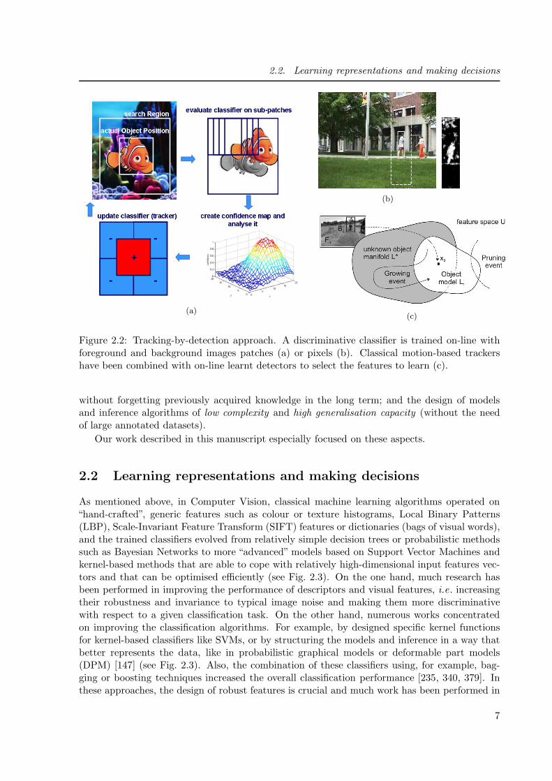
Figure 2.2: Tracking-by-detection approach. A discriminative classifier is trained on-line withforeground and background images patches (a) or pixels (b). Classical motion-based trackershave been combined with on-line learnt detectors to select the features to learn (c).
without forgetting previously acquired knowledge in the long term; and the design of modelsand inference algorithms of low complexity and high generalisation capacity (without the needof large annotated datasets).
Our work described in this manuscript especially focused on these aspects.
2.2 Learning representations and making decisions
As mentioned above, in Computer Vision, classical machine learning algorithms operated on“hand-crafted”, generic features such as colour or texture histograms, Local Binary Patterns(LBP), Scale-Invariant Feature Transform (SIFT) features or dictionaries (bags of visual words),and the trained classifiers evolved from relatively simple decision trees or probabilistic methodssuch as Bayesian Networks to more “advanced” models based on Support Vector Machines andkernel-based methods that are able to cope with relatively high-dimensional input features vec-tors and that can be optimised efficiently (see Fig. 2.3). On the one hand, much research hasbeen performed in improving the performance of descriptors and visual features, i.e. increasingtheir robustness and invariance to typical image noise and making them more discriminativewith respect to a given classification task. On the other hand, numerous works concentratedon improving the classification algorithms. For example, by designed specific kernel functionsfor kernel-based classifiers like SVMs, or by structuring the models and inference in a way thatbetter represents the data, like in probabilistic graphical models or deformable part models(DPM) [147] (see Fig. 2.3). Also, the combination of these classifiers using, for example, bag-ging or boosting techniques increased the overall classification performance [235, 340, 379]. Inthese approaches, the design of robust features is crucial and much work has been performed in
7

Chapter 2. Context
(a) (b)
Figure 2.3: Extracting “hand-crafted” low-level features and (a) forming codeword dictionaries(bags of visual words) or (b) learning Deformable Part Models (DPM).
the 1990s and 2000s to ”manually” create and refine such effective, invariant representations ofthe image data.
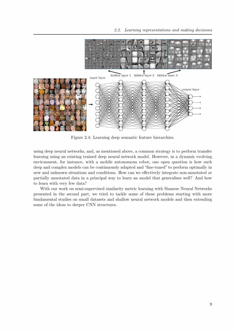
Convolutional Neural Networks (CNN), based on the fundamental work of K. Fukushima [152]and Y. LeCun [228], allow to overcome this manual feature design and learn discriminative fea-tures automatically from annotated data. Using neural architectures with several layers ofsubsequent convolution and pooling operations (and non-linear activation functions) togetherwith the Gradient Backpropagation algorithm thus results in a hierarchy of learnt feature ex-tractors from the lowest (pixel) to a higher (semantic) level (see Fig. 2.4). With the advent ofcheap GPU hardware and optimised software libraries in the 2010s, more complex models withmany layers have been used, and these deep neural networks achieved excellent performance onimage classification [161, 220] and have then been widely adopted for the majority of ComputerVision problems. Neural networks have a long history in Computer Vision, and their advan-tage is their flexibility in the model complexity that comes with different architectures, e.g . thenumber of layers, feature maps and neurons, optimised in a uniform way through Gradient Back-propagation, and especially their robustness to noise in the input data. Also, different trainingstrategies can be adopted depending on the amount of available annotated data and the natureof the given task to perform. Classically, neural networks has been trained in a supervisedway for classification problems. But, semi-supervised and weakly supervised algorithms exist aswell, e.g . with Siamese Neural Networks [99, 121]. With few labelled data, a common techniqueconsists in retraining or fine-tuning the last layer(s) of an existing deep neural network model,trained for example on an image classification problem with the ImageNet dataset [325] (transferlearning). When no labelled training data is available, one can use an unsupervised learningapproach with specific neural network architectures such as auto-encoders [187] and GenerativeAdversarial Networks (GAN) [163] to automatically extract high-level information for furtheranalysis. Recently, many variants of such deep neural network architectures, training algorithmsand loss functions have been proposed in the literature.
However, with deeper and more complex models come several difficulties and limitations. Oneproblem is over-fitting, that has either been addressed by specific regularisation techniques suchas DropOut or DropConnect or by increasing the training dataset and semi-supervised learningmethods. The lack of annotated training data is a frequent issue for many application when
8
2.2. Learning representations and making decisions
Figure 2.4: Learning deep semantic feature hierarchies.
using deep neural networks, and, as mentioned above, a common strategy is to perform transferlearning using an existing trained deep neural network model. However, in a dynamic evolvingenvironment, for instance, with a mobile autonomous robot, one open question is how suchdeep and complex models can be continuously adapted and “fine-tuned” to perform optimally innew and unknown situations and conditions. How can we effectively integrate non-annotated orpartially annotated data in a principal way to learn an model that generalises well? And howto learn with very few data?
With our work on semi-supervised similarity metric learning with Siamese Neural Networkspresented in the second part, we tried to tackle some of these problems starting with morefundamental studies on small datasets and shallow neural network models and then extendingsome of the ideas to deeper CNN structures.
9

Chapter 2. Context
10

3 Curriculum vitae
Stefan DUFFNER, born on the 15/02/1978 in Schorndorf (Germany).
Appointment and career:
Institution: INSA Lyon Grade: Maıtre de Conferences CNSince: 1st September 2012 CNU Section: 27eme sectionDepartement: 50% Premier Cycle (PC),50% Informatique
Laboratory: LIRIS
Professional address:
B: INSA LyonBatiment Blaise Pascal7 avenue Jean Capelle69621 Villeurbanne Cedex
T: +33 (0)4 72 43 63 65@: [email protected]
m: http://www.duffner-net.de
Education
2008 PhD in Computer Science from Freiburg University, Germany
Defended: 28/03/2008 Freiburg University, GermanyTitle: “Face Image Analysis with Convolutional Neural Networks”Funding: Orange LabsSupervision: Prof. Dr. Christophe Garcia (Orange Labs),
Prof. Dr. Hans Burkhardt (Freiburg University, Germany)
2004 Master’s degree in Computer Science (MSc), Freiburg University, Germany
1st year: Freiburg University, Germany
2nd year: Ecole Nationale Superieure d’Ingenieurs de Caen (ENSICAEN),GREYC, Image Team, Caen,Supervision Dr. Stephanie Jehan-Besson (GREYC)
Dr. Gerd Brunner (Freiburg University)
2002 Bachelor’s degree University of Applied Sciences, Constance, Germany
11

Chapter 3. Curriculum vitae
Professional Experience
since 2012 LIRIS/CNRS, Imagine team, INSA de Lyon
Associate Professor
Research topics: image classification, object detection and recognition, video analysis,visual object tracking, machine learning, neural networks
2008-2012 Idiap Research Institute, Martigny, Switzerland
Post-doctoral researcher in computer vision and object tracking in the context of theEuropean project TA2 (Together Anywhere, Together Anytime)Team Dr. Jean-Marc Odobez
2004-2007 Orange Labs, Rennes, France
PhD in the field of object detection in images and videos using machine learning.
PhD thesis: “Face Image Analysis with Convolutional Neural Networks”
Supervision Prof. Dr. Christophe Garcia (Orange Labs),Prof. Dr. Hans Burkhardt (Freiburg University, Germany)
Teaching
Recent teaching activities at the departments ”Premier Cycle”, ”Informatique” as well as”Telecommunications” at INSA Lyon :
1A PCC CM/TD/TP ”Algorithms and Programming”
2A PCC/SCAN CM/TD/TP ”Algorithms and Programming”, ”Introduction to Databases”
3IF CM/TD/TP ”Software engineering” (responsible of module)
3IF TD/TP ”Probability Theory”
3IF/4IF TP ”Operating Systems”
5IF CM/TP ”Big Data Analytics” / ”Machine Learning”
4TC CM/TP ”Image and Video Processing”
5TC (SJTU) CM/TP ”Computer Vision and Machine Learning”
5TC CM/TP ”Scientific Computing and Data Analytics”
Publications
See publication list on page 135.
12

Other responsibilities and activities
Teaching:
• Responsible of the Computer Science module of second year SCAN, INSA Lyon (Englishteaching)
• Responsible of the Software Engineering module at the third year IF (computer science)department of INSA Lyon
• Responsible of personalised curricula (parcours amenage) at IF department, INSA Lyon
• Member of the ATER candidate selection committee of INSA Lyon regarding the 27thCNU section (”Informatique”)
Research:
• Council member of the Lyon Computer Science Federation (”Federation Informatique deLyon”, FIL)
• Responsible of the topic ”Image and Graphics” of the FIL
• Expertises for ANR (and Swiss FNS) research project proposals and ANRT CIFRE appli-cations
• Numerous reviews for renowned journals and conferences (IEEE Transactions on PatternAnalysis and Machine Intelligence (PAMI), IEEE Transactions on Image Processing (IP),IEEE Transactions on Neural Networks and Learning Systems (NNLS), IEEE Transactionson Cybernetics (CYB), Pattern Recognition (PR) etc.)
• Co-organisation of a workshop on Deep Learning at the French conference RFIA 2017
• Co-organisation of a workshop on Neural Networks and Deep Learning (RNN) in Lyon2018
13

Chapter 3. Curriculum vitae
14
4 Overview of research work and
supervision
During the last 16 years, I conducted my research activities in five different academic andindustrial research institutions in France, Germany and Switzerland. They are mainly related tothe fields of computer vision, image and video analysis and machine learning, i.e. the automaticextraction, analysis and interpretation of semantic information from digital images and videos.
From 2002, I prepared my Master’s degree at the University of Freiburg in Germany, focusingon topics concerning image processing, artificial intelligence, robotics, machine learning andapplied mathematics. I performed part of my studies at the ENSICAEN in Caen, France,and my master thesis at the GREYC laboratory, on spatio-temporal object segmentation invideos. In 2004, I started my PhD research on Convolutional Neural Networks applied to faceimage analysis, at France Telecom R&D, Rennes, (now Orange Labs), and I defended it in thebeginning of 2008 at the Freiburg University. Between 2008 and 2012, I worked as a post-doctoralresearcher at the Idiap Research Institute in Martigny, Switzerland, on visual object trackingand probabilistic models for long-term multi-object face tracking. Since, 2012, I am a associateprofessor at INSA Lyon and the LIRIS laboratory, working on machine learning and computervision for various applications, such as object detection, tracking and recognition, and face andgesture analysis.
This rich experience from several scientific, social and cultural contexts gave me a broadrange of technical capacities and knowledge under diverse points of view and approaches, froma more specific to a more general level, professionally as well as personally.
In the following, I will briefly describe our research and my supervision work and, in thesucceeding chapters, go into more technical detail on the research we have conducted after myPhD thesis.
4.1 Convolutional Neural Networks for face image analysis
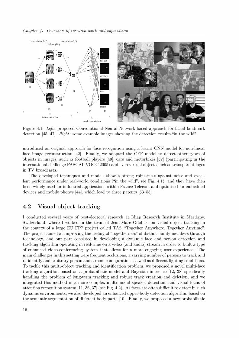
During my PhD [56], supervised by Christophe Garcia at France Telecom R&D, Rennes, (nowprofessor at LIRIS) and Prof. Dr. Hans Burkhardt at the University of Freiburg, Germany (nowemeritus professor), we worked on new Convolutional Neural Network (CNN) models for the au-tomatic analysis of faces in images. Our starting point was the well-known Convolutional FaceFinder (CFF) from Garcia and Delakis [156], and we proposed new neural architectures andlearning algorithms for different computer vision and face analysis problems. Our first contri-bution [45, 47, 50] concerned the automatic detection of facial feature points (facial landmarks)in face images in order to align the face to a canonical position for further processing (e.g . forrecognition) (see Fig. 4.1). Then, we proposed a novel CNN-based regression approach for au-tomatic face alignment that did not require an explicit detection of feature points [41]. We also
15
Chapter 4. Overview of research work and supervision
l5
l1
l3
subsamplingconvolution 7x7 convolution 5x5
l4
l2l6
nose
left eye
right eye
mouth
feature extraction
model association
Figure 4.1: Left: proposed Convolutional Neural Network-based approach for facial landmarkdetection [45, 47]. Right: some example images showing the detection results “in the wild”.
introduced an original approach for face recognition using a learnt CNN model for non-linearface image reconstruction [42]. Finally, we adapted the CFF model to detect other types ofobjects in images, such as football players [49], cars and motorbikes [52] (participating in theinternational challenge PASCAL VOCC 2005) and even virtual objects such as transparent logosin TV broadcasts.
The developed techniques and models show a strong robustness against noise and excel-lent performance under real-world conditions (“in the wild”, see Fig. 4.1), and they have thenbeen widely used for industrial applications within France Telecom and optimised for embeddeddevices and mobile phones [44], which lead to three patents [53–55].
4.2 Visual object tracking
I conducted several years of post-doctoral research at Idiap Research Institute in Martigny,Switzerland, where I worked in the team of Jean-Marc Odobez, on visual object tracking inthe context of a large EU FP7 project called TA2, “Together Anywhere, Together Anytime”.The project aimed at improving the feeling of “togetherness” of distant family members throughtechnology, and our part consisted in developing a dynamic face and person detection andtracking algorithm operating in real-time on a video (and audio) stream in order to built a typeof enhanced video-conferencing system that allows for a more engaging user experience. Themain challenges in this setting were frequent occlusions, a varying number of persons to track andre-identify and arbitrary person and a room configurations as well as different lighting conditions.To tackle this multi-object tracking and identification problem, we proposed a novel multi-facetracking algorithm based on a probabilistic model and Bayesian inference [12, 38] specificallyhandling the problem of long-term tracking and robust track creation and deletion, and weintegrated this method in a more complex multi-modal speaker detection, and visual focus ofattention recognition system [11, 36, 37] (see Fig. 4.2). As faces are often difficult to detect in suchdynamic environments, we also developed an enhanced upper-body detection algorithm based onthe semantic segmentation of different body parts [10]. Finally, we proposed a new probabilistic
16

4.2. Visual object tracking
Figure 4.2: Real-time on-line multi-face tracking in dynamic environments with an RGB camera.People may move freely in the room and leave and enter the scene. Left: The proposed algorithmtracks and re-identifies a varying number of persons over long time periods despite frequent falsedetections and missing detections. Right: integration in a multi-modal person and speakertracking and identification system.
Figure 4.3: Left: procedure of PixelTrack. Pixel-wise detection and segmentation is performedin parallel, and the two models are jointly learnt on-line. Right: particle filter-based MCTapproach, where a discriminative model is learnt on-line using negative examples from likelydistracting regions in the scene (blue rectangles).
face tracking method [40] that takes into account different visual cues (colour, texture, shape)and dynamically adapts the inference according to an integrated reliability measure.
Later, with Prof. Garcia at LIRIS, we continued our research on visual object tracking,but on more generic methods that track arbitrary single objects under challenging conditions,i.e. moving camera, difficult changing lighting conditions, deforming and turning objects, withother distracting objects etc. In this context, we developed several original methods. The firstone, called “PixelTrack” [5, 34], is based on a pixel-based Hough voting and a colour segmenta-tion model and is particularly well suited for fast tracking of arbitrary deformable objects (seeFig. 4.3). The second one, called “Motion Context Tracker” (MCT) [6, 31], is based on a particlefilter framework and uses a discriminative on-line learnt model to dynamically adapt to the scenecontext by taking into account other distracting objects in the background (see Fig. 4.3).
These different works on visual object tracking will be described in more detail in Part I ofthe manuscript.
17

Chapter 4. Overview of research work and supervision
Video
Tracker 1
Tracker 2
Tracker N
Scene Feature
Extraction
Hidden
Markov
Model
Kalman
Filter
Object
position
Scene Context
Classifier
Selection
of
tracker
Figure 4.4: Top: dynamic tracker selection algorithm based on a scene context classifier. Bottom:example video with tracking result of the proposed method. Different colours represent differenttrackers.
4.3 PhD thesis supervision
My supervision activities of PhD students began in 2012 when I joined the IMAGINE team ofthe LIRIS laboratory and INSA Lyon as associate professor.
From 2013 to 2016, I co-supervised the thesis of Salma Moujtahid [283] on visual objecttracking with Prof. Atilla Baskurt, and it was defended on 03/11/2016. We started from theobservation and hypothesis that some tracking algorithms perform better in a given environmentand others perform better in other settings. Thus, we developed a method [29] that, given a setof tracking algorithms running in parallel on a video, evaluates the confidence of each trackerand chooses the best one at each instant of the video stream according to an additional spatio-temporal coherence criterion. Further, we conceived a set of visual features that were ableto quantify the characteristics of the global scene context in a video at a given time. Usingthese scene context features, we trained a classifier that estimates with high precision the besttracker for a given visual context over time [28] (see Fig. 4.4). Using this tracker selectionalgorithm, we combined several state-of-the-art trackers operating on different (complementary)visual features, and achieved an improved performance. With this approach, we also participatedin the international Visual Object Tracking challenge, VOT 2015, where we obtained a goodranking among many powerful state-of-the-art methods [23].
From 2012, I also co-supervised the thesis of Samuel Berlemont [90] with Prof. ChristopheGarcia and Dr. Gregoire Lefebvre from Orange Labs, Grenoble. This industrial thesis wasdefended in February 2016 and concerned the development of new algorithms to automaticallyrecognise symbolic 3D gestures performed with a mobile device in the hand using inertial sensordata (see Fig. 4.5). We proposed a new model and a weakly supervised machine learningtechnique based on a Siamese neural network to learn similarities between gesture signals ina low-dimensional sub-space, achieving state-of-the-art recognition rates [2, 22, 24] comparedto previously proposed approaches, including our own method based on a CNN [33]. We not
18

4.3. PhD thesis supervision
Figure 4.5: Left: symbolic 3D gesture recognition with inertial sensor data from mobile devices.Right: proposed Siamese neural network architecture learning similarities and dissimilaritiesfrom tuples of input samples and using a polar sine-based objective function.
MappingFunction
)(⋅f
MappingFunction
)(⋅fW
ix
Cost / Loss Function
Attract a similar pairSeparate a dissimilar pair
iy
),(a Wxf ii = ),(b Wyf ii =
Original Space
Target Space
)(⋅J
hese.pdf
Figure 4.6: Left: Siamese neural network architecture learning a similarity metric in the featurespace. Right: similar and dissimilar (face) pairs used for training (LFW dataset).
only showed an increased rejection performance for unknown gestures, but also and improvedclassification rate with a specific neural network structure learning from tuples of data samples(instead of pairs or triplets as in previous approaches) and a novel polar sine-based objectivefunction (see Fig.4.5), which leads to a better training stability and a better modelling of therelation between similar and dissimilar training examples.
I further co-supervised the thesis of Lilei Zheng [441], defended on 10/05/2016, togetherwith Atilla Baskurt, Khalid Idrissi and Christophe Garcia. In this work, we introduced severalnew similarity metric learning methods [4, 8, 26, 27], based on linear and non-linear projectionsthrough Siamese Multi-Layer Perceptrons, and applied them to the problem of face verification,i.e. given two (unknown) face images, deciding if they belong to the same (unknown) personor not (see Fig. 4.6). The first method that we proposed for training these Siamese neuralnetwork models is called Triangular Similarity Metric Learning (TSML) [4, 26] and is basedon an objective function using the cosine distance and conditions the norm of the projectedfeature vectors, thus improving the convergence and overall performance of this learnt metric.The second method is called Discriminative Distance Metric Learning (DDML) [4] and uses theEuclidean distance and a margin to define the objective function for training the model, givingcomparable performance to TSML. We further evaluated the proposed methods on the problem
19

Chapter 4. Overview of research work and supervision
Figure 4.7: Proposed orientation-specific re-identification deep neural network. Left: in thefirst step, the two neural network branches are pre-trained separately on identity labels andbody orientations (supervised learning). Right: in the second step, the whole neural network isfine-tuned for person re-identification (triplet learning with hard negative selection).
of speaker verification (i.e. audio signals) and also achieved state-of-the-art results. Finally, weapplied our TSML algorithm on kinship verification [25], i.e. verifying parent-child relationshipsin images, and participated in an international competition organised at the FG conference in2015, and our approach was ranked first in one of the sub-competitions and second in the otherone.
From 2015 to 2018, I co-supervised the thesis of Yiqiang Chen [116] together with Prof.Atilla Baskurt and Jean-Yves Dufour from Thales ThereSIS Lab, Paris, and it was defendedon the 12/10/2018. The topic of the thesis was ”person re-identification in images with DeepLearning”, which is a similar problem to the above-mentioned face verification, i.e. given twoimages of (unknown) persons (pedestrians), e.g . coming from different cameras, we want to knowif they belong to the same person or not. Because the identities of the persons are generally notknown before building the model and because we want the method to be as generic as possible,we tackled this problem with a similarity metric learning approach, as is commonly done in theliterature. To this end, we proposed several deep learning-based approaches, where the similaritylearning is generally performed with a variant of the Siamese neural network using triplets ofexamples instead of pairs, i.e. one reference example (or anchor), one similar example and onedissimilar example.
First, we developed a CNN-based discriminative algorithm to automatically recognise pedes-trian attributes, i.e. semantic mid-level descriptions of persons, such as gender, accessories,clothing etc. [15]. These attributes are helpful to describe characteristics that are invariant topose and viewpoint variations. Then we combined this model with another CNN trained forperson identification, and the two branches are fine-tuned for the final person re-identificationtask [20]. Secondly, among the challenges, one of the most difficult is the variation under differentviewpoints. To deal with this issue, we propose an orientation-specific deep neural network [17](see Fig. 4.7), where one branch performs body orientation regression and steers another branchthat learns separate orientation-specific layers. The combined orientation-specific CNN featurerepresentations are then used for the final person re-identification task. Further, developed an-
20

4.3. PhD thesis supervision
other approach to include visual context into the re-identification process [16], i.e. for a givenperson query image, we additionally used the image region of the surrounding persons to computea pairwise combined distance measure based on an location-invariant group feature representa-tion. Finally, as a fourth contribution in this thesis, we proposed a novel listwise loss functiontaking into account the order in the ranking of gallery images with respect to different probeimages [18]. Further, an evaluation gain-based weighting is introduced in the loss function todirectly optimise the evaluation measures of person re-identification.
Currently, there are four ongoing PhD theses at LIRIS that I actively co-supervise :
• Paul Compagnon, “Prediction de routines situationnelles dans l’activite des personnesfragiles”, co-supervision with Christophe Garcia (LIRIS) and Gregoire Lefebvre (OrangeLabs Grenoble),
• Thomas Petit, “Reconnaissance faciale a large echelle dans des collections d’emissions detelevision”, co-supervision with Christophe Garcia (LIRIS) and Pierre Letessier (InstitutNational de l’Audiovisuel),
• Guillaume Anoufa, “Reconnaissance d’objets intrus en phase de vol helicoptere par Ap-prentissage Automatique”, co-supervision with Christophe Garcia (LIRIS) and NicolasBelanger (Airbus Helicopters)
• Ruiqi Dai, “Apprentissage autonome pour la vision intelligente”, co-supervision with VeroniqueEglin (LIRIS) and Mathieu Guillermin (Institut Catholique de Lyon)
21

Chapter 4. Overview of research work and supervision
22

PART I
On-line learning and applications to
visual object tracking
23


5 Multiple object tracking in
unconstrained environments
5.1 Introduction
Visual object tracking consists in following a given object in an image sequence or video overtime. The object to follow is usually given, the first time it is visible in the video, by a humanor an automatic detection algorithm. If a detection algorithm is used, applying it to every frameof the video is generally not an acceptable or sufficient solution as the object may not always bedetected, false detections may occur, previous detections are not taken into account such thata certain continuity is lacking and, finally, running the detector may be computationally tooexpensive. The output of tracking algorithms is a description of the state of the object at eachpoint in time in the video. This can be its position and scale in the image (usually describedas a bounding box), or a “real-world” position (2D on the ground plane, or 3D), but also itsorientation, speed or a finer description such as a parametric shape or part-based model.
Tracking can be performed off-line or on-line. In off-line tracking, the entire video is availableat once for analysis and inference, whereas in on-line tracking, a video stream is analysedsequentially from the beginning, i.e. at each point in time only the past and present informationcan be used to estimate the object state but not the future. We will only consider on-linetracking in this work.
Finally, an important aspect of tracking algorithms concerns the number of objects to track.If we know that there is only one object to track, and it is visible throughout the whole video,Single Object Tracking (SOT) approaches are used. In that case, the algorithm is given thestate (e.g . the bounding box) of the object in the beginning, and it is supposed to track it untilthe end. We will come back to SOT in chapter 6. In Multiple Object Tracking (MOT), severalobjects (usually of the same category) are to be followed in an image sequence, and state-of-theart tracking algorithms mostly rely on a separate object detector trained (off-line) for the givencategory of objects to track (e.g . a person, face or car detector).
This presents a certain number of inherent challenges:
• in most applications, the number of visible objects is not known a priori , and the algorithmneeds to handle newly arriving and disappearing objects,
• objects may occlude each other partially or completely,
• the object detector may miss objects, and false detections may occur,
• the algorithm may confuse two objects, e.g . when they come close to each other (track IDswitch).
25
Chapter 5. Multiple object tracking in unconstrained environments
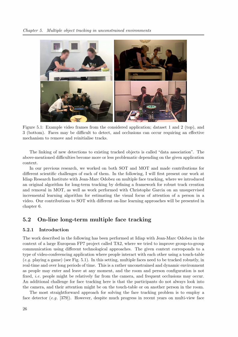
Figure 5.1: Example video frames from the considered application; dataset 1 and 2 (top), and3 (bottom). Faces may be difficult to detect, and occlusions can occur requiring an effectivemechanism to remove and reinitialise tracks.
The linking of new detections to existing tracked objects is called “data association”. Theabove-mentioned difficulties become more or less problematic depending on the given applicationcontext.
In our previous research, we worked on both SOT and MOT and made contributions fordifferent scientific challenges of each of them. In the following, I will first present our work atIdiap Research Institute with Jean-Marc Odobez on multiple face tracking, where we introducedan original algorithm for long-term tracking by defining a framework for robust track creationand removal in MOT, as well as work performed with Christophe Garcia on an unsupervisedincremental learning algorithm for estimating the visual focus of attention of a person in avideo. Our contributions to SOT with different on-line learning approaches will be presented inchapter 6.
5.2 On-line long-term multiple face tracking
5.2.1 Introduction
The work described in the following has been performed at Idiap with Jean-Marc Odobez in thecontext of a large European FP7 project called TA2, where we tried to improve group-to-groupcommunication using different technological approaches. The given context corresponds to atype of video-conferencing application where people interact with each other using a touch-table(e.g . playing a game) (see Fig. 5.1). In this setting, multiple faces need to be tracked robustly, inreal-time and over long periods of time. This is a rather unconstrained and dynamic environmentas people may enter and leave at any moment, and the room and person configuration is notfixed, i.e. people might be relatively far from the camera, and frequent occlusions may occur.An additional challenge for face tracking here is that the participants do not always look intothe camera, and their attention might be on the touch-table or on another person in the room.
The most straightforward approach for solving the face tracking problem is to employ aface detector (e.g . [379]). However, despite much progress in recent years on multi-view face
26

5.2. On-line long-term multiple face tracking
detection, these methods are mostly employed in scenarios where people predominantly looktowards the camera. As we demonstrate in our results, this is not sufficient for more complexscenarios, where faces are missed around 30 − 40% of the time due to less common head poses.Unfortunately, the difficult head postures can last for relatively long periods of time (up toone minute in some of our videos). This means that face detection algorithms have to becomplemented by robust tracking approaches; not only to interpolate detection results or filterout spurious detection, as is often assumed, but also to allow head localisation over extendedperiods of time.
Numerous multiple faces tracking methods have been proposed in the literature (e.g . [93,142, 269, 304, 405]), mainly focusing on new features, new multi-cue fusion mechanisms, betterdynamics or adaptive models for instance [58, 74, 164, 326], and results are demonstrated mostlyon short sequences [58, 74, 164, 326].
However, very few of them address track initialisation and termination, especially in termsof performance evaluation. A face detector is often used to initialise new tracks, but how tocope with its uncertain output? A high confidence threshold may lead to missing an earlytrack initialisation. Conversely, with a low threshold false tracks are likely to occur. Tracktermination can be even more difficult. How do we know at each point in time if a tracker isoperating correctly? This is an important issue in practice, especially since an incorrect failuredetection can lead to losing a person track for a long time until the detector finds the face again.
5.2.2 State of the art
Many existing MOT approaches operate off-line, i.e. the information from the entire video isavailable for the inference, or sometimes these methods are applied on sliding time windowsin order to allow for a “pseudo”-on-line operation. In most of these works, data association isformulated as a global optimisation problem on a graph-based representation [88, 102, 181, 281,309, 433]. However, these off-line algorithms are not suited for the real-time on-line setting thatwe investigated here.
In on-line MOT, existing approaches either employ deterministic methods for data associa-tion [75, 215] based on the Hungarian algorithm [286] or on a greedy approach [98] or probabilisticmethods, like the traditional Multiple Hypothesis Tracker (MHT) [317], the Joint ProbabilisticData Association Filter (JPDAF) [149], both based on a Kalman Filter framework, and ParticleFilter-based techniques [185, 202, 214, 295, 297, 412].
Most of these methods do not explicitly incorporate mechanisms for track creation anddeletion, especially with longer periods of missed detections and frequent false detections, asis the case in the application scenario that is considered here. Principled methods exist tointegrate track creation and termination within the tracking framework, for example Reversible-Jump Markov Chain Monte Carlo (RJ-MCMC) [214, 417]. But to be effective, they requireappropriate global scene likelihood models involving a fixed number of observations (independentfrom the number of objects), and these are difficult to build in multi-face tracking applications.
Kalal et al . [205] present an interesting approach for failure detection in visual object trackingthat is based on the idea that a correctly tracked target can be tracked backwards in time.Unfortunately, the backward tracking greatly increases the overall computational complexity(by a factor that is linear in the backward depth). In a particle filter tracking framework,another solution is to directly model a failure state as a random variable within the probabilisticmodel [310]. However, this increases the complexity of the model and thus the inference, and itis difficult, in practice, to model the distribution of a failure state or failure parameters. Closerto our work, Dockstader et al . [137] proposed to detect failure states in articulated human body
27

Chapter 5. Multiple object tracking in unconstrained environments
tracking using a Hidden Markov Model (HMM). However, their method differs significantly fromours: they only use one type of observation (the state covariance estimate) which in our caseproves to be insufficient for assessing tracking failure; their observation are quantised to use astandard discrete multinomial likelihood model, whereas our method learns these likelihoods ina discriminative fashion; and their HMM structure (number of states, connections) is specificallydesigned for their articulated body tracking application.
In applications that are similar to ours, the problem of deciding when to stop tracking a faceis usually solved in a recursive manner. This means, assessing tracking failure is often left tothe (sudden) drop of objective or likelihood measures which are not easy to control in practice[279, 280].
In many scenarios of interest, the camera is fixed, and due to the application and the roomconfiguration, people in front of the camera tend to behave similarly over long periods of time.However, most of the existing tracking methods ignore this long-term information, as theyconcentrate on video clips that are often not longer than a minute. Or if they use long-terminformation, it is mainly for constructing stable appearance models of tracked objects [200, 428],e.g . by working at different temporal scales [364]. Similarly, some methods [74, 203] train an(object-specific) detector online, during tracking, to make it more robust to short-term andlong-term appearance changes. However this increases the computational complexity, becausea separate model has to be built for each person, and each such detector has to be applied onthe input frames. Mikami et al . [279] introduced the Memory-based Particle Filter where ahistory of past states (and appearances [280]) is maintained and used to sample new particles.However, they only addressed single, near-frontal face tracking, in high resolution videos and onlyevaluated the method on 30 to 60-second video clips. Other works (e.g . [221, 249, 347]) tacklethe problem of long-term person tracking by analysing the statistics of features from shortertracks (tracklets), and by proposing methods to effectively associate them. These algorithmsare different from ours as they process the data off-line, i.e. the observations at each point intime are known in advance, and they mainly deal with tracking the position of the full humanbody as opposed to just faces. Another approach for multiple pedestrian tracking [86] associatessmaller tracklets on-line and in a statistical sampling framework but no principled mechanism forstarting and ending tracks is proposed. Recently, and after our work, an approach similar to oursfrom Xiang et al . [407] has been proposed, using Markov Decision Processes and re-inforcementlearning for data association, and to decide on track deletion.
In the following, we will first introduce the principal framework and equations for MOTwith particle filters and Markov Chain Monte Carlo (MCMC) sampling, and then describe ourcontributions related to the probabilistic framework of track creation and removal, long-termstatic and dynamic observation models as well as experimental results [12, 38].
5.2.3 Proposed Bayesian multiple face tracking approach
We tackle the problem of multi-face tracking in a recursive Bayesian framework. Assumingwe have the observations Y1:t from time 1 to t, we want to estimate the posterior probabilitydistribution over the state Xt at time t:
p(Xt|Y1:t) =1
Cp(Yt|Xt)×
∫
Xt−1
p(Xt|Xt−1)p(Xt−1|Y1:t−1) dXt−1 , (5.1)
where C is a normalisation constant. As closed-form solutions are usually not available inpractice, this estimation is implemented using a particle filter with a Markov Chain MonteCarlo (MCMC) sampling scheme [214]. The main elements of the model are described below.
28

5.2. On-line long-term multiple face tracking
5.2.3.1 State space
We use a multi-object state space formulation, with our global state defined as Xt = (Xt,kt),where Xt = Xi,ti=1..M and kt = ki,ti=1..M . The variable Xi,t denotes the state of face i,which comprises the position, speed, scale and eccentricity (i.e. the ratio between height andwidth) of the face bounding box. Each ki,t denotes the status of face i at time t, i.e. ki,t = 1 ifthe face is visible at time t, and ki,t = 0 otherwise. Finally, M denotes the maximum numberof faces visible at a current time step.
5.2.3.2 State Dynamics
The overall state dynamics, used to predict to current state from the previous one, is defined as:
p(Xt|Xt−1) ∝ p0(Xt|kt)∏
i∈1..M|ki,t=1
p(Xi,t|Xi,t−1) , (5.2)
that is the product of an interaction prior p0 and of the dynamics of each individual face thatis visible at iteration t like in tracking methods for a fixed number of targets [214]. Note thatthis is actually feasible since the creation and deletion of targets are defined outside the filteringstep (see next section). The position and speed components of the visible faces are describedby a mixture of a first-order auto-regressive model pa and a uniform distribution pu, i.e., if xdenotes a position and speed component vector, we have: p(xi,t|xi,t−1) = αpa(xi,t|xi,t−1) + (1−α)pu(xi,t|xi,t−1), with pa(xi,t|xi,t−1) = N (Axt−1; 0,Σ), and pu(xi,t|xi,t−1)) = c with c being aconstant allowing for small “jumps” coming from face detection proposals (see Eq. 5.8). A firstorder model with steady-state is used for the scale and eccentricity parameters. If x denotesone such component: (xt − SS) = N (a(xt−1 − SS); 0, σSS), where SS denotes the steady-statevalue. The steady-state values for scale and eccentricity are updated only when a detected faceis associated with the face track and at a much slower pace compared to the frame-to-framedynamics.
The interaction prior p0 is defined as
p0(Xt|kt) =∏
i,j∈P
φ(Xi,t,Xj,t) ∝ exp− λg
∑
i,j∈P
g(Xi,t,Xj,t), (5.3)
preventing targets to become too close to each other. The set P consists of all possible pairs
of objects that are visible. The penalty function g(Xi,t,Xj,t) =2a(Bi∩Bj)a(Bi)+a(Bj )
is the intersection
area as a fraction of the average area of the two bounding boxes Bi and Bj defined by Xi,t andXj,t, where a(.) denotes the area operator. The factor λg controls the strength of the interactionprior (set to 5 in our experiments).
5.2.3.3 Observation Likelihood
As a trade-off between robustness and computational complexity, we employ a relatively simplebut effective observation likelihood for tracking. Another model could be used as well.
Given our scenario, we assume that the face observations Yi,t are conditionally indepen-dent given the state, leading to an observation likelihood defined as the product of the visibleindividual faces likelihoods:
p(Yt|Xt) =∏
i|ki,t=1
p(Yi,t|Xi,t). (5.4)
29

Chapter 5. Multiple object tracking in unconstrained environments
Note that we did not include a partial (or full) overlap model in the likelihood component,nor any other contextual tracking techniques [414]. Strong overlaps are prevented explicitly bythe interaction term (Eq. 5.3) in the dynamics. This approach is appropriate for our scenarios(teleconference, HCI/HRI), where continuous partial face occlusions happen only rarely. Moreoften, faces are occluded by other body parts that are not followed by the tracker, like a person’shand, or another person’s body crossing in front. Even a joint likelihood model would not handlethese cases. Thus, for longer full occlusions, our strategy is to have the algorithm remove thetrack of the occluded face, and restart it afterwards as soon as possible.
The observation model for a face i is based on R = 6 HSV colour histograms Yi,t =[h(r,Xi,t)] (r = 1..R), that are computed on the face region described by the state Xi,t. Theyare compared to histogram models h∗i,t(r), to define the observation likelihood for a tracked faceas follows:
p(Yi,t|Xi,t) ∝ exp(−λD
6∑
r=1
(D2[h∗i,t(r), h(r,Xi,t)]
)−D0) , (5.5)
where D denotes the Euclidean distance , λD = 20, and D0 is a constant offset defining thedistance at which the likelihood in Eq. (5.5) gives 1.0. More precisely, we divided the face intothree horizontal bands and in each band computed two normalised histograms with two differ-ent levels of quantisation. Specifically, we used the scheme proposed in [304] which decouplescoloured pixels (put into Nb×Nb HS bins) from grey-scale pixels (Nb separate bins) and appliedit with two different quantisation levels, Nb = 8 and Nb = 4 bins per channel. This choiceof semi-global multi-level histograms results from a compromise between speed, robustness toappearance variations across people as well as head pose variations for individuals, and a wellconditioned likelihood, i.e. peaky enough to accept a well identified optimum, but with a smoothbasin of attraction towards this optimum, adapted to low sampling strategies.
The histogram models of one face are initialised when a new target is added to the tracker.Furthermore, to improve the tracker’s robustness to improper initialisation and changing lightingconditions, they are updated whenever a detected face is associated with the given face track(see below):
h∗i,t(r) = (1− ǫ)h∗i,t−1(r) + ǫhdi,t(r) ∀r , (5.6)
where hdi,t denotes the histograms from the detected face region, and ǫ is the update factor (setto 0.2 in our experiments).
5.2.3.4 Tracking algorithm
At each time instant, the tracking algorithm proceeds in two main stages: first, recursivelyestimate the states of the currently visible faces relying on the model described above andsolved using an MCMC sampling scheme. Second, make a decision on adding a new face or ondeleting currently tracked faces. This second stage is described in Section 5.2.4. The MCMCsampling scheme allows for efficient sampling in this high-dimensional state space of interactingtargets, and follows the method described in [214].
Let N be the total number of particles and Nbi the number of “burn-in” particles. At eachtracking iteration, we do:
1. initialise the MCMC sampler at time t with the sample X(0)t obtained by randomly selecting
a particle from the set X(s)t−1, s = (Nbi + 1) . . . N at time t − 1 and sample the state of
every visible target i using the dynamics p(Xi,t|Xi,t−1) (deleted targets are ignored);
30

5.2. On-line long-term multiple face tracking
2. sample iteratively N particles from the posterior distribution of (5.1) using the Metropolis-Hastings algorithm:
(a) sample a new particle Xt′from a proposal distribution q(Xt
′|Xt(s)
) (described below);
(b) compute the acceptance ratio:
a = min
(1,
p(Xt
′|Y1:t) q(Xt
(s)|Xt
′
)
p(Xt
(s)|Y1:t) q(Xt
′|Xt
(s))
)(5.7)
(c) accept the particle (i.e. define Xt(s+1)
= Xt′) with probability a. Otherwise, add the
old particle (i.e. set Xt(s+1)
= Xt(s)
)
After time step t, the particle set X(s)t Ns=Nbi+1 represents an estimation of the posterior
p(Xt|Y1:t).The proposal function q(·) allows for selecting good candidates for the particle set. Efficiency
in MCMC sampling is obtained by modifying object states one at a time. More precisely, a new
sample is selected by letting Xt′= Xt
(s), randomly select a face i amongst the visible ones, and
then sample the proposed state X′i,t of face i from:
q(X′i,t|Xt) =
[(1− α)
1
N −Nbi
∑
r
p(X′i,t|X
(s)i,t−1) + αp(X′
i,t|Xdt )]
(5.8)
that is a mixture of the state dynamics (ensuring temporal smoothness) and the output of a facedetector (avoiding tracker drift) controlled by the factor α, where Xd
t denotes the state of theclosest detection coming from a face detector [379] and associated with face i. Again, targetsremoved at the previous step are ignored, while recently added targets are simply sampledaround their initial position.
5.2.4 Target creation and removal
The way objects are added and removed from the tracker is a key feature of the algorithm thatwe proposed. In our application scenario, the goal is to avoid false alarms as much as possible.This means, the tracker should be able to detect as quickly as possible if there is a trackingfailure. On the other hand, it should not stop tracking when there is no failure since it may takea long time until the object is detected again.
We proposed to use two different Hidden Markov Models (HMM) for that purpose, as de-scribed in the following sections. One is used for object creation and the other for object removal.Each of them receives different types of observations.
A face detector (for both frontal and profile views) is called every 10 frames (i.e. aroundtwice per second, as our algorithm is able to process around 20-23 frames/s in real-time). TheHMMs are updated only at these instants, but rely on observations computed on all frames sincethe last update. According to our experiments, applying the detector to every video frame didnot significantly improve the tracking performance and considerably slowed down the algorithm.
Before the creation and removal step, each detection is associated to a track provided thefollowing conditions hold:
1. the detection is not associated with any other target,
2. it has the smallest distance to the tracked target,
31

Chapter 5. Multiple object tracking in unconstrained environments
ctct−1
oct,1 oct,2 oct,Nc
Figure 5.2: The HMM used at each image position for tracker target creation. The variablect indicates a face centred at a particular image position. The probability of ct is estimatedrecursively using the observations oct,1..o
ct,Nc
.
3. the distance between detection and target is smaller than two times the average width oftheir bounding boxes,
4. the two bounding boxes overlap.
Although a more generic way would be to use training data to learn the association rules andparameters as done in [322], for instance, the above conditions work well for our data in thelarge majority of cases.
In the following, we describe the HMMs for target creation and removal. Note that naturally,only un-associated detections are considered for the initialisation of a new target.
5.2.4.1 Creation
When initialising a new target we have two objectives: first, minimise erroneous initialisationsdue to false detections, and second, initialise correct targets as early as possible.
For deciding when to add new targets to the face tracker, we propose a simple HMM thatestimates the probability of a hidden, discrete variable ct(i, j) indicating at each image position(i, j) if there is a face or not at this position. Figure 5.2 illustrates the model. In the following, wedrop the indices (i,j) for clarity. Let us denote by Oc
t = [oct,1, . . . , oct,Nc
] the set of Nc observationsat each time step t, and by Oc
1:t = [Oc1, . . . ,O
ct ] the sequence of observations from time 1 to time
t. Assuming the transition matrix is defined as: p(ct|ct−1) = 1 iff ct = ct−1 and 0 otherwise, theposterior probability of the state ct can be recursively estimated as:
p(ct = s|Oc1:t) =
p(Oct |ct = s) p(ct−1 = s|Oc
1:t−1)∑s′ p(O
ct |ct = s′) p(ct−1 = s′|Oc
1:t−1), (5.9)
wherep(Oc
t |ct) =Nc∏
i=1
p(oct,i|ct) . (5.10)
Track creation: for each detected face that is not associated with any current face target, wedecide whether a track is created or not. To this end, if (i, j) denotes the centre position of theface detection, the ratio:
rct (i, j) =p (ct(i, j) = 1|Oc
1:t(i, j))
p (ct(i, j) = 0|Oc1:t(i, j))
(5.11)
is computed. If rct (i, j) > 1, then a new track is initialised at (i, j). Otherwise, no track iscreated from the given detection.
32
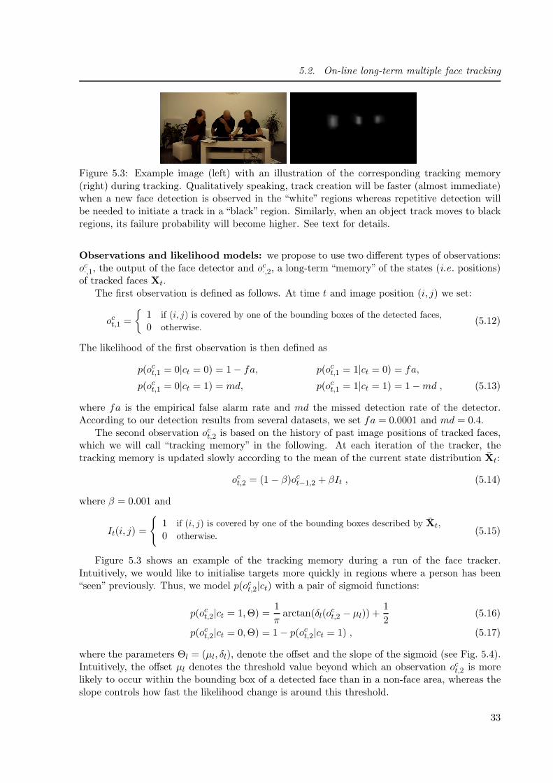
5.2. On-line long-term multiple face tracking
Figure 5.3: Example image (left) with an illustration of the corresponding tracking memory(right) during tracking. Qualitatively speaking, track creation will be faster (almost immediate)when a new face detection is observed in the “white” regions whereas repetitive detection willbe needed to initiate a track in a “black” region. Similarly, when an object track moves to blackregions, its failure probability will become higher. See text for details.
Observations and likelihood models: we propose to use two different types of observations:oc·,1, the output of the face detector and oc·,2, a long-term “memory” of the states (i.e. positions)of tracked faces Xt.
The first observation is defined as follows. At time t and image position (i, j) we set:
oct,1 =
1 if (i, j) is covered by one of the bounding boxes of the detected faces,
0 otherwise.(5.12)
The likelihood of the first observation is then defined as
p(oct,1 = 0|ct = 0) = 1− fa, p(oct,1 = 1|ct = 0) = fa,
p(oct,1 = 0|ct = 1) = md, p(oct,1 = 1|ct = 1) = 1−md , (5.13)
where fa is the empirical false alarm rate and md the missed detection rate of the detector.According to our detection results from several datasets, we set fa = 0.0001 and md = 0.4.
The second observation oct,2 is based on the history of past image positions of tracked faces,which we will call “tracking memory” in the following. At each iteration of the tracker, thetracking memory is updated slowly according to the mean of the current state distribution Xt:
oct,2 = (1− β)oct−1,2 + βIt , (5.14)
where β = 0.001 and
It(i, j) =
1 if (i, j) is covered by one of the bounding boxes described by Xt,0 otherwise.
(5.15)
Figure 5.3 shows an example of the tracking memory during a run of the face tracker.Intuitively, we would like to initialise targets more quickly in regions where a person has been“seen” previously. Thus, we model p(oct,2|ct) with a pair of sigmoid functions:
p(oct,2|ct = 1,Θ) =1
πarctan(δl(o
ct,2 − µl)) +
1
2(5.16)
p(oct,2|ct = 0,Θ) = 1− p(oct,2|ct = 1) , (5.17)
where the parameters Θl = (µl, δl), denote the offset and the slope of the sigmoid (see Fig. 5.4).Intuitively, the offset µl denotes the threshold value beyond which an observation oct,2 is morelikely to occur within the bounding box of a detected face than in a non-face area, whereas theslope controls how fast the likelihood change is around this threshold.
33

Chapter 5. Multiple object tracking in unconstrained environments
0
0.25
0.5
0.75
1
0 0.2 0.4 0.6 0.8
likel
ihoo
d
observationdecisionboundary
p(oi|k = 0,Θ)p(oi|k = 1,Θ)
pos. training observationsneg. training observations
Figure 5.4: Example of an observation likelihood model (here or3) described by a pair of sigmoidfunctions with learnt parameters Θ = δ, µ. The parameters of the positive sigmoid function(solid red curve) have been optimised to model best the positive (blue solid boxes) and nega-tive (purple dotted boxes) training observations (here illustrated by histograms) according toEq. 5.18. The offset µ (here at x = 0.29), where the two sigmoid paired curves cross, defines asoft decision boundary.
Parameter learning: the parameters Θl = (δl, µl) of the sigmoid functions in equations 5.16and 5.17 have been trained offline with a set of N± observations oi. These observations aretracking memory values that have been collected from real tracking sequences and are composedof N+ positive instances measured at image positions of correct face detections, and N− negativeinstances measured at image positions of false detections. To train the model, we maximise theposterior probability of the labels for the given observations o:
Θ∗ = argmaxΘ
N±∏
i=1
p(c = Ci|oi,Θ), (5.18)
where Ci ∈ 0, 1 denotes the class label of oi, and p(c = ci|oi,Θ) ∝ p(oi|c = ci,Θ) is given byEq. 5.16 and 5.17, and we assumed an equal prior on both classes. In practise, we find a goodapproximation of Θ∗ by doing a grid search in a reasonable range over the parameter space Θ.Figure 5.4 shows an example of a pair of learnt sigmoid functions and the respective decisionboundary (in this case for target removal).
If observations are greater than µ, the ratio p(oi|c=1)p(oi|c=0) > 1, that means a face is more likely to
be present. Otherwise, it is more likely that no face is present.
5.2.4.2 Removal
During tracking, we want to assess at each point in time if the algorithm is still correctlyfollowing a face or if it has lost track. The algorithm can lose track, for example, when it getsdistracted by a similar background region or when a person leaves the scene. More concretely,the objective is to interrupt the tracking as soon as possible if a failure occurs, and to continuetracking otherwise, even when a face has not been detected and associated with the track for along time.
In a way similar to target initialisation, we propose to use for each tracked face i an HMMestimating at each time step t the hidden status variable ki,t indicating correct tracking (ki,t = 1)
34

5.2. On-line long-term multiple face tracking
ktkt−1
ort,1 ort,2 ort,Nr
Figure 5.5: The HMM for target removal, used for each tracked face. The variable kt indicatesif a given face is still tracked correctly or if a failure occurred. The probability of kt is estimatedrecursively using the observations ort,1..o
rt,Nr
.
or tracking failure (ki,t = 0). We will drop the face index i in the following. Figure 5.5 illustratesthe proposed model.
Let us denote by Ort = [ort,1, . . . , o
rt,N2] the set of Nr observations at each time step t, and by
Or1:t = [Or
1, . . . ,Ort ] the sequence of observations from time 0 to time t. The posterior probability
of kt can be recursively estimated as:
p(kt|Or1:t) =
∑k′t−1
p(Ort |kt) p(kt|k′t−1) p(k
′t−1|Or
1:t−1)∑k′t,k
′t−1
p(Ort |k′t) p(k′t|k′t−1) p(k
′t−1|Or
1:t−1), (5.19)
wherep(Or
t |kt) =Nr∏
i=1
p(ort,i|kt) . (5.20)
The state transition probability p(kt|kt−1) is set to 0.999 for staying in the same state and 0.001for changing state, assuming a frame rate of approximately 20 frames per second as in ourexperiments.
Track ending: for each tracked face and at each time step, we compute the ratio:
rkt =p(kt = 1|Or
1:t)
p(kt = 0|Or1:t)
. (5.21)
If rkt < 1 for a given face, then the tracking is considered to have failed and the target is removed.
Observations and likelihood models: we propose to use Nr = 7 different types of observa-tions Or
t = [ort,1, . . . , ort,7] extracted from the image as well as the state of the tracker itself. We
can divide them into two categories:
• four static observations (ort,1, . . . , ort,4) that provide indications on the state of the tracker,
and
• three dynamic observations (ort,5, . . . , ort,7) that provide indications on the temporal evolu-
tion and variability of certain observations.
Except for one observation, all likelihoods are modelled by pairs of sigmoid functions:
p(ort,i|kt = 1,Θ) = ai arctan(δi(ort,i − µi)) +
1
2, (5.22)
p(ort,i|kt = 0,Θ) = 1− p(ort,i|kt = 1), (5.23)
where, as for target creation observations (section 5.2.4.1), the amplitude ai is set to1π (or − 1
πfor some observation types), and the parameters Θi = (δi, µi), i.e. the slope and the offset of the
35
Chapter 5. Multiple object tracking in unconstrained environments
sigmoid, have been trained offline with a set of positive and negative observations as describedat the end of Section 5.2.4.1. The only difference is that the training observations are collectedat each time instant during tracking runs and not only when faces are detected. Below, wedescribe each observation we have used and comment on the learnt parameters.Static observations: the first static observation for a given target is based on the output of theface detector:
ort,1 =
1 if a detection is associated with the target
0 otherwise.(5.24)
The likelihood p(ort,1|kt) is defined in the same way as for oct,1 in Eq. 5.13 (that is,p(ort,1 = u|kt = l) = p(oct,1 = u|ct = l)).
The second observation ort,2 is the tracking memory value at the respective target position(m,n) in the image, as defined in the previous section (Eq. 5.14 and 5.15):
ort,2 = oct,2(m,n) . (5.25)
This ensures that the tracking of a face is more likely to be maintained if a face stays at itsprevious position (with a high tracking memory value). And conversely, the target should beremoved with a higher probability when it moves to image regions that were never occupied bya face before.
The third observation type is the tracker observation likelihood computed at the mean statevalue Xi,t of target i:
ort,3 = p(Yi,t|Xi,t) , (5.26)
as defined by Eq. 5.5. The likelihood p(ort,3|kt) is again defined by a pair of sigmoids (Eq. 5.22and 5.23).
The fourth observation relates to the variance of the target filtering distribution. Moreprecisely, let σ2
i,t,x and σ2i,t,y be the variances of the horizontal and vertical position of target
state Xi,t. Then we defineort,4 = max(σ2
i,t,x, σ2i,t,y). (5.27)
A higher variance of the state distribution means a higher uncertainty (and vice versa), and thetrack should be stopped more quickly.Dynamic observations: the three remaining observations are based on the temporal variation ofdifferent features. They rely on the detection of rapid increases or decreases over time of particlevariance and observation likelihood. To this end, we assume that the values of these features arenormally distributed during tracking, and we use the Page-Hinckley test [82] to detect jumpsor drops of these (one-dimensional, Gaussian) “signals” with respect to their means. This testworks as follows: let ωt be the signal for which we want to detect an abrupt decrease. Then, thefollowing values are computed at each iteration t:
Mω,t = Mω,t−1 +
(ωt − (ωt −
jω2)
)(5.28)
mω,t = max(mω,t−1,Mω,t) (5.29)
mω,t = mω,t −Mω,t , (5.30)
where Mω,0 = 0, jω is a constant that determines the tolerated change of value ω, and ωt isthe running average of ω. Mω,t accumulates the values going above the expected lower bound(ω − jω). The value mω,t memorises the maximum value of this cumulative sum, and thedifference between these last two values mω,t (Eq. 5.30) is an indication of an abrupt decrease of
36

5.2. On-line long-term multiple face tracking
0
0.5
1
1.5
2
2.5
3
3.5
4
0 2 4 6 8 10 12 14 16 18 20
t
ω
ω
ω − jω2
mω
Figure 5.6: Illustration of the Page-Hinckley test to detect abrupt decreases of a signal. Thesolid red line shows the temporal evolution of some signal, the purple dotted line shows thecomputed result of the Page-Hinckley test that we use as observation to detect abrupt signaldrops. At time t = 14 a drop of the signal occurs and is correctly detected (peak of purpledotted line).
the value ω. On the other hand, if ωt decreases only gradually, then the running average ωt willfollow this decrease. The cumulative sum Mω,t will constantly increase, leading to mω,t = Mω,t
and thus mω,t = 0. Figure 5.6 illustrates the Page-Hinckley test with some example data.
Similarly, for detecting an abrupt increase of ω we compute:
Uω,t = Uω,t−1 +
(ωt − (ωt +
jω2)
)(5.31)
uω,t = min(uω,t−1, Uω,t) (5.32)
uω,t = Uω,t − uω,t , (5.33)
where Uω,0 = 0. In its original form, the Page-Hinckley test produces a binary output. It is oneif mω,t or uω,t is above a predefined threshold and zero otherwise. Here, we propose to directlyuse the values mω,t or uω,t as observations.
Thus, using equations 5.28-5.33, we define:
ort,5 = mort ,3 ort,6 = mort ,4 ort,7 = uort ,4 . (5.34)
Observations ort,5 indicate drops of the likelihood p(Yt|Xt) of a given face (see 5.26). And ort,6,ort,7 indicate abrupt decreases and increases of the variance of the state distribution defined in5.27. The likelihood functions p(ort,5|kt), p(ort,6|kt), and p(ort,7|kt) are defined by pairs of sigmoids(Eq. 5.22, 5.23) with parameters trained offline.
5.2.5 Re-identification
Our algorithm further tries to keep track of the identities of different persons and associates eachtrack with a person, i.e. for each new target track it decides if it belongs to a previously seenperson or if it is an new person. In this work, we built person models which are longer-termdescriptions of person appearance acquired from observations during the tracking process. Here,a simple colour-based model, similar to [364] has been used. More specifically, the model Pj,t of
a person j is composed of two colour histograms: one describing the face region, hfj,t, and one
37

Chapter 5. Multiple object tracking in unconstrained environments
for the shirt, hsj,t. The structure of the histograms is similar to the one used for the observationlikelihood in the tracking algorithm (5.2.3.3), i.e. two different quantisation levels and decoupledcolour and grey-scale bins.
If a target is added to the tracker and there is no stored person model that is un-associated,a new model is initialised immediately and associated to the target. Otherwise, the face andshirt histograms (hfi,t, h
si,t) of the new target i are computed recursively over r successive frames
and stored in P ∗i,t. After this period, we calculate the likelihood of each stored model Pj,t given
an unidentified candidate P ∗i,t:
p(Pj,t|P ∗i,t) = exp
(−λ(wfD
2[hfj,t, hfi,t] + wsD
2[hsj,t, hsi,t])), (5.35)
where D is the Euclidean distance, and the weights are wf = 1, ws = 2. A given person i is thenidentified by simply determining the model Pm,t with the maximum likelihood:
m = argmaxj
p(Pj,t|P ∗i,t) , (5.36)
provided that p(Pm,t|P ∗i,t) is above a threshold θ (we chose 0.1 here). If not, a new person
model is created and added to the stored list. All associated person models are updated at eachiteration with a small factor αp = 0.01. The candidate models are updated with factor α∗ = 0.1.
5.2.6 Experiments
Experiments have been conducted on more than 9 hours of video data that have been annotatedextensively. We used three sets of videos recorded in different environments (see Fig. 5.1).According to our scenario, recorded people have been sitting at a table and filmed by a centralcamera (roughly 2-3 metres away). They have been playing online games with people in a remotelocation using a laptop or touch-screen. As a result, they are often looking downwards and theirfaces are often not detected by a standard detector [379].
The principal performance measures are precision and recall (over time) of the face trackingresult, as we want to track faces as long as possible (to obtain a high recall) and stop trackingas soon as a failure occurs (to increase the precision). The recall and false positive rate for anentire video are defined as:
R =
∑Gi=2 δidi∑Gi=2 δi
, FP =
∑Gi=2 δifi∑Gi=2 δi
, (5.37)
where G is the number of annotated frames, di the proportion of correctly tracked/detectedfaces in frame i (i.e. those for which F > 0.1), fi is the number of false positive outputs dividedby the number of ground truth objects in frame i, and δi is the time difference between frame iand i− 1.
We also measure the total number of interruptions for a given dataset. An interruption isdefined as the event when a track is falsely ended, i.e. the face (ground truth) is still presentbut the respective target is removed from the tracker.
Finally, to measure the accuracy of identification as described section 5.2.5, we computedthe object purity [345] for each ground truth object:
OP =
∑Gi=2 δiqi∑Gi=2 δi
, (5.38)
38

5.2. On-line long-term multiple face tracking
where G is again the number of annotated frames, and qi is the proportion of correctly identifiedfaces in frame i, as explained in the following. The identity assigned to a ground truth objectat time i is given by the algorithm described in 5.2.5 and more specifically Eq. 5.36. Once thetracking has been run on a complete video, we can compute the above rate by associating to eachobject the face track that has the longest overlap with the object (according to the F-measure).
We compared our results against a standard face detector [379] including models for frontaland profile views, with two competitive baselines:
• RJ-MCMC : a tracker based on the Reversible-Jump Monte Carlo Markov Chain algorithm[214, 417]. In addition to the Update move, which follows the MCMC description in section5.2.3.4, four other moves have been implemented to handle the creation and removal oftargets: Add, Delete, Stay, and Leave. For more details, we refer the reader to [214, 417].
• MCMC baseline: an MCMC-based tracker, i.e. the algorithm described in section 5.2.3.For target creation and removal, the following strategy has been used: every (un-associated)face detection is initialised as a new target. We also tried to initialise a target only af-ter several successive detections but this didn’t have a large impact on the precision. Atracked target was removed if it had no associated detections for 100 frames (8 seconds)or if the likelihood dropped below 10% of its running average.
Table 5.1 compares the algorithms for a given face detector threshold. The proposed methodoutperforms the others for all three datasets. Since the tracking algorithm for the MCMCbaseline is the same as for the proposed method, the performance improvement is clearly dueto our proposed target creation and removal mechanisms. The precision of RJ-MCMC is ratherlow because the creation and removal of targets is only based on the observation likelihood, as in[214]. Note that, unlike our approach, RJ-MCMC adds and removes targets at the particle level.Although this is a principled statistical framework that models at each point in time the currentbelief on the number of visible targets, it is more difficult to capture longer-term dynamics andfeatures from the state distribution itself. The MCMC baseline, on the other hand, adds andremoves targets based on more efficient, longer-term observations, namely the likelihood withrespect to its mean and the face detector output. Thus, its performance is better than the oneof RJ-MCMC. Also, the total number of tracker interruptions is decreased. This means that theproposed method maintains face tracks longer, even when the face detector provides no outputfor extended periods of time or when the likelihood is temporarily decreasing.
Figure 5.7 shows some tracking results of a video from dataset 3 containing 3-4 persons. Thepeople change their seats from time to time, occlusions occur, and head poses can be challenging,as illustrated in the example.
More explanation and results can be found in [12, 38].
5.2.7 Conclusion
We have proposed a Bayesian framework for long-term, on-line MOT including a learnt trackcreation and removal approach to explicitly handle inherent weaknesses of object detectionalgorithms. Our experiments showed that the precision and recall with our tracking algorithmis considerably increased. We want to note that we also successfully applied our algorithm tolong-term SOT, as well as to other scenarios related to Human-Robot Interaction, involvingseveral people interacting with a robot [12]. Further, other existing algorithms could largelybenefit from our track creation and removal framework, when applied on a longer time scale.Also, in the future, other types of long-term cues could be included in the proposed framework,
39

Chapter 5. Multiple object tracking in unconstrained environments
data face RJ-MCMC MCMC oursset detection baseline
1recall 55.0% 89.5% 85.2% 93.9%FP rate 2.00% 20.75% 4.29% 1.45%# interrupt. − 861 395 112average OP − 41.35% 68.69% 68.98%
2recall 39.9% 75.7% 69.9% 76.0%FP rate 0.41% 3.27% 1.21% 0.77%# interrupt. − 2062 1004 567average OP − 49.09% 66.61% 69.60%
3recall 48.3% 77.2% 75.1% 93.7%FP rate 0.33% 18.2% 1.06% 1.19%# interrupt. − 1299 455 166average OP − 27.96% 34.23% 57.46%
Table 5.1: Performance comparison with the proposed multiple face tracking framework on thethree datasets.
(a) frame 20000 (b) frame 20038 (c) frame 52408 (d) frame 114870
(e) frame 114948 (f) frame 114962 (g) frame 115148 (h) frame 115302
Figure 5.7: Snapshots of tracking results on dataset 3. Different coloured rectangles representdifferent identities (purple: face detector). Top: MCMC baseline, bottom: proposed approach.With the baseline method, some target are initialised from false detections 5.7(b), 5.7(g), andtracks are not maintained when detections are missing 5.7(c). Our approach avoids false initial-isations and maintains good tracks longer. In 5.7(f) failures are detected earlier, and in 5.7(h),the lost target is re-initialised earlier (second person from the left).
40

5.3. Visual focus of attention estimation
Figure 5.8: Graphical illustration of VFOA estimation in one of the investigated settings (ameeting room). Targets 1 to 4 are persons, 5 corresponds to the table.
There are still some limitations of the proposed framework. Even if we are able to accuratelyand quickly detect failures, the result is still dependent on the time it takes to obtain a new facedetection to reinitialise the tracking. Thus, having less tracking failures and better multi-viewdetectors is obviously a way to increase the performance. In our given face-tracking scenario,we could also apply different detectors based on the head, upper-body or full body, and combinethe results for a more robust result. In this regard, we have conducted some work on improvingthe precision of upper-body detection by including semantic colour segmentation in existingtexture-based models [10].
5.3 Visual focus of attention estimation
5.3.1 Introduction
The approach I presented in the previous section is able to detect, re-identify and track personsin front of a camera. It is often necessary to further analyse the behaviour of the persons in agiven scene. In particular, one wants to know what they are looking at, at any given point intime, i.e. what they are paying attention to in terms of their eye gaze. This can be an object oranother person and is called the Visual Focus Of Attention (VFOA) (see Fig. 5.8)
Similar to our previous work on face tracking, we place this problem in a dynamic con-text, where the actual number of present persons is not fixed, and where their positions andthe configuration of the room and furniture are not constrained. In this type of environment,many existing approaches fail, as they rely on a certain proximity to the camera or more spe-cific hardware (depth and/or infra-red sensors). We have proposed an original algorithm thatautomatically and incrementally learns models for VFOA recognition from video data, and thusis independent from a given room or person configuration.
5.3.2 State of the art
In principle, the VFOA of a person can be determined by the person’s eye gaze direction. Manystudies about automatic gaze estimation from video exist [153, 268, 282, 387, 388, 396], buttheir use is mostly limited to close-up and near-frontal views of a person’s face, for example inHuman-Computer Interaction applications. Other works [138, 380, 381] rely on the fusion ofinformation from several cameras. But often the spatial camera configuration is very constrained
41

Chapter 5. Multiple object tracking in unconstrained environments
or a preceding calibration step is required, which can be difficult or even impossible dependingon the application and environment. Also depth sensors, like Kinect, have been used for headpose and eye gaze estimation [153]. Although, their precision depends highly on the distance ofthe person from the sensor, this is an interesting direction for future research beyond the scopeof this work. In our work, we have focused on (non-intrusive) scenarios where a single camera isfixed at a few meters from the filmed persons and where the persons stay roughly at the sameplaces most of the time, like in formal meetings or video-conferencing applications (as illustratedin Fig. 5.8).
Previous work on VFOA analysis in such open spaces has mostly been based on the estimationof head pose as a surrogate for gaze [67, 69, 71, 83, 87, 110, 225, 299, 308, 344, 352, 354, 355,381, 429]. This is done either globally, e.g . by learning to classify image patches of the headat different angles based on low-level visual features or locally, i.e. by localising certain facialfeatures [318, 411] and by geometrically and statistically inferring the global orientation, ora combination of the two [67] (see [287] for a literature survey). However, these algorithmsmostly require the person(s) to face the camera more or less and be rather close to it in orderto have a relatively high image resolution of the face. Using video, head pose estimation canbe included in a joint head and pose tracking algorithm [69, 226, 262, 321]. Early works ofStiefelhagen and Zhu [353], for example, used a Gaussian Mixture Model (GMM) on head poseangles to estimate VFOA. The model is initialised with k-means and further updated withan Expectation-Maximisation algorithm. They also showed that using the other participant’sspeaking status increases the VFOA performance. Note that, in our work, we have concentratedon methods that are relying on visual information, although there are previous works that useaudio, actions or or types of cues to infer the VFOA [73, 300, 344, 353]. Otsuka and Yamato[299] proposed a method based on a Dynamic Bayesian Network (DBN) that also analyses thegroup behaviour and detects certain conversational patterns. A GMM and Hidden MarkovModel (HMM) approach for modelling and recognising VFOA was proposed by Smith et al .[346] for people walking by an outdoor advertisement and by Ba and Odobez [71] for analysingmeeting videos. In the latter work, the authors also presented a MAP adaptation method toautomatically adapt the VFOA model to the individual persons as well as a geometrical model(based on findings from [151, 177]) combining head orientation and eye gaze direction. Voit andStiefelhagen [381, 382] built on this geometrical model and presented VFOA recognition resultson a dynamic dataset with multiple cameras. Later, Ba and Odobez [72] extended their approachon VFOA estimation for meetings with a DBN that incorporates contextual information, likespeaking status, slide change, and modelling conversation behaviour. Dong et al . [138] proposedan approach also based on a DBN which is similar to ours in the fact that they recognise VFOAby comparing tracked face image patches with a set of clusters modelling the face appearancefor each attention target. However, the difference to our approach is that the clusters in theiralgorithm are trained before the tracking and in a supervised way. Thus, the number of targetsand the targets itself are known in advance.
The work of Benfold et al . [87] is similar to ours in that they also perform unsupervisedtraining on head images in order to determine where people look at in a given video. However,their approach is not incremental (although they claim that it could be extended) and needs aninitial training of prior models using hand-labelled ground plane velocities and gaze directionsof persons in a given video. They do not extract VFOA but head orientation (using a givennumber of classes), and they apply their approach to video surveillance data where they takeadvantage of people moving, which is different from our indoor scenario. On the one hand,the advantage of their probabilistic model – a conditional random field (CRF) – is that a morepowerful discriminative head pose classifier can be learnt taking into account several hidden
42

5.3. Visual focus of attention estimation
variables (walking speed, angle velocities etc.). On the other hand, the complexity of learningand inference is increased, and the model is also independent from the head tracking as opposedto our approach that allows for a purely sequential and joint inference.
As experimental results of these previous works show, head pose can be used effectively toestimate the VFOA of a group of people, e.g . in a meeting room, to a certain extend. However,there are certain drawbacks of this approach: for example, in uncontrolled environments it isdifficult to estimate head pose reliably because it often requires a large amount of annotatedtraining data of head appearances or shapes beforehand in order to model all the possiblevariations of a head and face among different people as well as for a given individual. Thesedata are often not available, or too time-consuming to produce. Further, for accurate headpose estimation results, a relatively precise localisation of the head, the face, or facial features– commonly called face alignment – is crucial but challenging in unconstrained applicationscenarios.
Another difficulty in automatic VFOA estimation is to determine the number of semanticvisual targets for a given person in a video and to map them to given head pose or eye gazeangles. A preceding supervised training step is commonly performed on separate video data,and in some approaches the model (e.g . a GMM) is adapted on-line to a given video. However,it is desirable to avoid this scene-dependant training step or in some applications it might evenbe impossible. Further, the subsequent model adaptation can in many cases not cope with adifferent number of focusing targets or when the persons’ locations differ too much from thosein the training data.
We proposed a novel approach that alleviates these problems. Our algorithm, given a videostream from a single camera and the rough 2D position estimation of a person’s head, incremen-tally learns to automatically extract the VFOA of the person without explicitly estimating headpose or gaze and without any prior model of the head, face, the room configuration, or otherexternal conditions. The proposed method learns on-line the different classes of targets in anunsupervised way directly from the low-level visual features. This means also that, as opposedto supervised algorithms, it will not assign labels to the different targets (e.g .’table’, ’screen’,’person 1’). However, we will experimentally show that the proposed unsupervised approach isable to identify and estimate the (unlabelled) targets with higher accuracy than a classical su-pervised approach. The fact that no pre-trained model is needed makes this approach especiallyinteresting for applications where the specific environment, as well as the configuration of theroom and the filmed persons is not known a priori , and where an explicit training phase is notpossible.
5.3.3 Face and VFOA tracking
The principal procedure of our approach is illustrated in Fig. 5.9. First, a basic tracking algo-rithm is initialised and tracks a rectangular face region throughout the video stream. The imagepatch inside the tracked face region is extracted and visual features are computed to initialisethe VFOA model at the first video frame and to update it at each subsequent frame during thetraining phase (see section 5.3.4). An incremental clustering algorithm on these low-level fea-tures is used to learn face appearances corresponding to attention targets of the person. At thesame time a matrix modelling the transition probabilities between the different targets is learnt,and together with the clusters forms a continuous HMM. Note that the learning is performedon-line and does not require any prior knowledge on head pose or room configuration.
After a given number of iterations (a couple of minutes from the beginning of a video) thetraining phase stops and the Particle Filter continues to jointly track face position and VFOA
43

Chapter 5. Multiple object tracking in unconstrained environments
Particle Filter:face and VFOA
tracking
HMMtraining
video stream
face image patches
VFOA model
face position + VFOA
Figure 5.9: Principal procedure of the VFOA learning and tracking approach.
of a person using the learnt HMM model, i.e. the transition probabilities and the face clusters.In order to facilitate understanding, before describing the main contribution of this work,
i.e. the unsupervised VFOA learning, we will first explain the underlying tracking framework inthe following section.
For tracking the face position and VFOA of a person, we used the Sequential Monte Carloalgorithm, commonly known as Particle Filter (c.f . [12, 304, 321]). It provides a solution for theclassical recursive Bayesian model, where, assuming we have the observations Y1:t from time 1to t, we estimate the posterior probability distribution over the state Xt at time t:
p(Xt|Y1:t) =1
Cp(Yt|Xt)×
∫
Xt−1
p(Xt|Xt−1)p(Xt−1|Y1:t−1) dXt−1 , (5.39)
where C is a normalisation constant. For simplicity and more principled evaluation, we onlyconsider the tracking of a single face in a video, although our approach can easily be extendedto multiple faces using an MCMC sampling approach (c.f . section 5.2.3) and thus be integratedin our MOT framework described in the previous section.
In our experiments, the state Xt = (Xt, v) is composed of the state of the face Xt = (x, y, s)with x, y being its position and s being its bounding box scale factor, as well as the currentVFOA target index v ∈ 1..V .
The dynamics of the face state p(Xt|Xt−1) are defined by a first-order auto-regressive modelwith Gaussian noise:
p(Xt|Xt−1) = N (Xt−1; 0,Σp) . (5.40)
The dynamics of the discrete VFOA target index v are defined by transition probability matrix
A := [aij ], i, j = 1..V with
aij := p(vt = j|vt = i) (5.41)
being the transition probability from VFOA target i to j. The co-variance matrix Σp =diag(σpx, σpy, σps) of the auto-regressive model is fixed, whereas the matrix A is learnt onlineduring the tracking of a person in a given video stream (see section 5.3.4.2).
The observations likelihood is defined as the product of a colour likelihood and texturelikelihood:
p(Yt|Xt) = p(YCt |Xt)p(Y
Tt |Xt) , (5.42)
where the colour likelihood is used to track the position and size (x, y, s) of the face boundingbox, and the texture likelihood is mainly used to track the VFOA target v. We define:
p(YCt |Xt) ∝ exp
(−λ1
9∑
r=1
(D2
C [h∗r , hr(Xt)]
))
, (5.43)
44

5.3. Visual focus of attention estimation
(a) (b)
Figure 5.10: Visual feature extraction for the VFOA model. a) HOG features are computed on agrid of 4×4 cells placed on the tracked face. b) To compute the histograms, gradient orientationis quantised into 4 bins (respectively 8 bins) and magnitude into 2 bins.
where λ1 is a constant, hr(Xt) are HSV colour histograms extracted from a grid of r = 9 cellscentred at Xt, h
∗r is the reference histogram initialised from the face region in the first frame,
and DC is the Bhattacharyya distance. As in [304], the histogram bins for the H and S channelsare decoupled from the V channel. Also the quantisation is applied at two different levels, i.e. 4bins and 8 bins, to improve the robustness under difficult lighting conditions. This leads to anoverall colour observation vector size of 9 · (8 · 8 + 8 + 4 · 4 + 4) = 828.
The texture likelihood is defined similarly:
p(YTt |Xt) ∝ exp
(−λ2
16∑
r=1
(DT [µr,v, tr(Xt)]
))
, (5.44)
where λ2 is a constant, tr(Xt) are Histograms of Oriented Gradients (HOG) (see descriptionbelow) extracted (similarly to hr) from a grid of 16 cells (indexed by r) centred at Xt, andµr,v are the reference histograms corresponding to the VFOA target index v in Xt. The overalltexture model is composed of a set of N -dimensional clusters with means µr,i where each clusteri ∈ 1..V corresponds to a VFOA target. DT is the normalised Euclidean distance:
DT (µr,i, tr(Xt)) =
√√√√N∑
j=1
(tr,j(Xt)− µr,i,j)2
σ2j + ǫ
, (5.45)
with ǫ being a small constant avoiding division by zero.The feature vectors tr(Xt) constitute the visual observations used for recognising the VFOA
targets of a person in a video by means of p(YT |Xt). They are computed on a 4 by 4 grid of non-overlapping cells on a face image patch as illustrated in Fig. 5.10(a). For each cell, two normalisedtwo-dimensional histograms of unsigned oriented gradients and magnitudes are computed usinga specific quantisation scheme illustrated in Fig. 5.10(b). The gradient orientation is quantisedin 4 bins and the magnitude in 2 bins. An additional bin (with no orientation) is used for veryweak gradients (in the centre of the half circle in the diagram). Also, to improve the overallrobustness and discriminative power, we compute two histograms at different quantisation levelsfor orientation: 4 and 8, and normalise each of them separately. Thus, the dimension N of thefeature vector is: 16 ·(4 ·2+1+8 ·2+1) = 416. One advantage of these histogram features is thatthey are relatively robust to small spatial shifts of the overall bounding box, which frequentlyoccur with common face tracking methods.
5.3.4 Unsupervised, incremental VFOA learning
The VFOA model can be regarded as a dynamic HMM estimating the hidden variable v, theVFOA target index, from the observed features tr(Xt), illustrated in Fig. 5.11. It consists of
45

Chapter 5. Multiple object tracking in unconstrained environments
vt−1 vt
tt−1 tt
A
Figure 5.11: The Hidden Markov Model used to estimate the hidden discrete variable v (theVFOA target) from the observations tt (feature vectors) using the learnt transition probabilitymatrix A.
two main parts. First, the data model that is used for the likelihood computation in Eq. 5.44and that contains the k cluster means µi and a global co-variance matrix Σ, and second, thematrix A (Eq. 5.41) defining the transition probabilities from one cluster to another. All, theseparameters are learnt on-line during the training phase, and used subsequently in the tracking(c.f . section 5.3.3). After training, the learnt parameters µi, Σ, and A of the HMM are used inthe Particle Filter framework explained in the previous section to jointly estimate the posteriorprobability of the state Xt at each time step. In the following, the training procedures aredescribed in more detail.
5.3.4.1 Clustering algorithm
The visual feature vectors tr(Xt) computed on the image region corresponding to the mean stateof the current distribution at time t are used to incrementally learn the VFOA classes. To thisend, we propose a specific sequential k-means clustering algorithm with an adaptive number ofclusters. The algorithm constructs a model of k clusters corresponding to the VFOA classesand described by their mean feature vectors µr,i (i = 1..k) and a global diagonal co-variancematrix Σ = diag(σ1, . . . , σN ). For better readability, in the following notation, we drop theindexes for the cell r and the time step t, denoting the current cluster means as µi and thecurrent feature vector as t. Algorithm 1 summarises the main learning procedure. At each timestep the observed feature vector t is computed, and the closest cluster c is determined using thenormalised Euclidean distance (Eq. 5.45). Also, the mean distance DT between each of the kclusters is calculated, and a new cluster is created if the distance of the current feature vector tothe closest cluster is greater than θcDT , where θc is a parameter of our algorithm (set to 2 in ourexperiments). Then, the mean vector µc of the closest cluster as well as the global covariancematrix Σ are incrementally updated using the current feature vector t. Finally, pairs of clustersare merged together if the distance of their means are below the threshold θdDT (with θd = 0.01in our experiments). At each time step, the algorithm classifies the observed features t fromthe mean state of a face into one of the k clusters: c, and, as we will show with the followingexperimental results, the learnt classes correspond to a large degree to specific targets of VFOA.
5.3.4.2 VFOA transition model
The transition probability matrix A of equation 5.41 is learnt on-line during the training phaseat the same time as the cluster centres. The main procedure is the following. The visual featurevectors t of the image patch corresponding to the current mean state are extracted, and theclosest cluster ct according to the normalised Euclidean distance (Eq. 5.45) is computed. Then,the transition probabilities act−1,j := p(v = j|v = ct−1) are linearly updated, using the following
46

5.3. Visual focus of attention estimation
Algorithm 1 Incremental VFOA clustering algorithm
k = kini Σ = Σini µi = t0 ni = 0 (i = 1..k)for t = 1 to T do
c = argmini(DT (t,µi)) ⊲ get closest cluster
DT = 2N(N+1)
∑k
i=1
∑k
j=i+1(DT (µi,µj))
if DT (t,µc) > θcDT then ⊲ add new cluster
k ← k + 1
nk = 1
µk = t
else
nc ← nc + 1 ⊲ update closest cluster
µc ← µc +1nc
(t− µc)
end if
incrementally update Σ
for each cluster pair (i,j) do ⊲ merge clusters
if DT (µci,µcj
) < θdDT then
µi = (niµi + njµj)/(ni + nj)
ni = ni + nj
remove cluster j
k ← k − 1
end if
end for
end for
equation:act−1,j = γ1j=ct + (1− γ)act−1,j ∀j ∈ 1..k, (5.46)
where 1x denotes the indicator function, and the constant γ = 0.001. Thus, the transitionprobability from ct−1 to ct is increased, and from ct−1 to any other cluster j is decreased. Also,a new row and column is added if a new cluster is created and inversely if a cluster is removed.At the end of each iteration, the row ct−1 that has been updated is normalised to sum up to 1.0.Algorithm 2 summarises the overall procedure. In many cases, the learnt transition matrix will
Algorithm 2 Incremental learning of the transition matrix
initialise A to uniform distribution: aij =1k i, j ∈ 1..k
for t = 1 to T doadapt the size of A to k × kct = argminiD(t,µi)act−1,j = γ1j=ct + (1− γ)act−1,ct
normalise row ct−1 to sum up to 1.0end for
have high values on the diagonal (staying in the same state most of the time) and low valueselsewhere. Of course, this depends on the dynamics of the scene. In our formal meeting setting,people are interacting frequently and changing their attention targets quite often. Thus, thisseems not to be a limitation. But even in more static settings (e.g . a person giving a talk), thismodel is still appropriate. And we can observe this with less active persons in some videos in
47
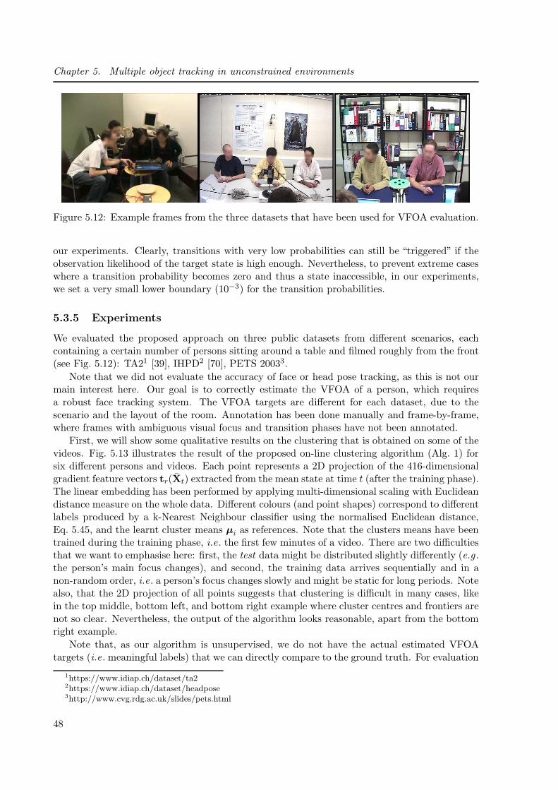
Chapter 5. Multiple object tracking in unconstrained environments
Figure 5.12: Example frames from the three datasets that have been used for VFOA evaluation.
our experiments. Clearly, transitions with very low probabilities can still be “triggered” if theobservation likelihood of the target state is high enough. Nevertheless, to prevent extreme caseswhere a transition probability becomes zero and thus a state inaccessible, in our experiments,we set a very small lower boundary (10−3) for the transition probabilities.
5.3.5 Experiments
We evaluated the proposed approach on three public datasets from different scenarios, eachcontaining a certain number of persons sitting around a table and filmed roughly from the front(see Fig. 5.12): TA21 [39], IHPD2 [70], PETS 20033.
Note that we did not evaluate the accuracy of face or head pose tracking, as this is not ourmain interest here. Our goal is to correctly estimate the VFOA of a person, which requiresa robust face tracking system. The VFOA targets are different for each dataset, due to thescenario and the layout of the room. Annotation has been done manually and frame-by-frame,where frames with ambiguous visual focus and transition phases have not been annotated.
First, we will show some qualitative results on the clustering that is obtained on some of thevideos. Fig. 5.13 illustrates the result of the proposed on-line clustering algorithm (Alg. 1) forsix different persons and videos. Each point represents a 2D projection of the 416-dimensionalgradient feature vectors tr(Xt) extracted from the mean state at time t (after the training phase).The linear embedding has been performed by applying multi-dimensional scaling with Euclideandistance measure on the whole data. Different colours (and point shapes) correspond to differentlabels produced by a k-Nearest Neighbour classifier using the normalised Euclidean distance,Eq. 5.45, and the learnt cluster means µi as references. Note that the clusters means have beentrained during the training phase, i.e. the first few minutes of a video. There are two difficultiesthat we want to emphasise here: first, the test data might be distributed slightly differently (e.g .the person’s main focus changes), and second, the training data arrives sequentially and in anon-random order, i.e. a person’s focus changes slowly and might be static for long periods. Notealso, that the 2D projection of all points suggests that clustering is difficult in many cases, likein the top middle, bottom left, and bottom right example where cluster centres and frontiers arenot so clear. Nevertheless, the output of the algorithm looks reasonable, apart from the bottomright example.
Note that, as our algorithm is unsupervised, we do not have the actual estimated VFOAtargets (i.e. meaningful labels) that we can directly compare to the ground truth. For evaluation
1https://www.idiap.ch/dataset/ta22https://www.idiap.ch/dataset/headpose3http://www.cvg.rdg.ac.uk/slides/pets.html
48
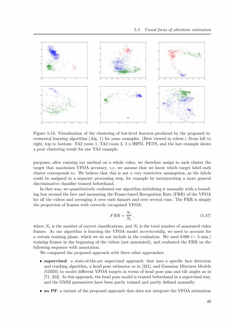
5.3. Visual focus of attention estimation
-0.5 0 0.5 1 1.5-1.5
-1
-0.5
0
0.5
1
-0.8 -0.6 -0.4 -0.2 0 0.2 0.4 0.6 0.8-1
-0.5
0
0.5
1
1.5
2
-0.8 -0.6 -0.4 -0.2 0 0.2 0.4 0.6 0.8-1
-0.5
0
0.5
1
-0.4 -0.2 0 0.2 0.4 0.6 0.8-1
-0.5
0
0.5
1
-1.5 -1 -0.5 0 0.5 1-1
0
1
2
3
-1 -0.5 0 0.5 1-1.5
-1
-0.5
0
0.5
1
Figure 5.13: Visualisation of the clustering of low-level features produced by the proposed in-cremental learning algorithm (Alg. 1) for some examples. (Best viewed in colour.) From left toright, top to bottom: TA2 room 1, TA2 room 2, 2 x IHPD, PETS, and the last example showsa poor clustering result for one TA2 example.
purposes, after running our method on a whole video, we therefore assign to each cluster thetarget that maximises VFOA accuracy, i.e. we assume that we know which target label eachcluster corresponds to. We believe that this is not a very restrictive assumption, as the labelscould be assigned in a separate processing step, for example by incorporating a more generaldiscriminative classifier trained beforehand.
In that way, we quantitatively evaluated our algorithm initialising it manually with a bound-ing box around the face and measuring the Frame-based Recognition Rate (FRR) of the VFOAfor all the videos and averaging it over each dataset and over several runs. The FRR is simplythe proportion of frames with correctly recognised VFOA:
FRR =Nc
Nt, (5.47)
where Nc is the number of correct classifications, and Nt is the total number of annotated videoframes. As our algorithm is learning the VFOA model incrementally, we need to account fora certain training phase, which we do not include in the evaluation. We used 8 000 (∼ 5 min.)training frames in the beginning of the videos (not annotated), and evaluated the FRR on thefollowing sequence with annotation.
We compared the proposed approach with three other approaches:
• supervised: a state-of-the-art supervised approach, that uses a specific face detectionand tracking algorithm, a head pose estimator as in [321], and Gaussian Mixtures Models(GMM) to model different VFOA targets in terms of head pose pan and tilt angles as in[71, 353]. In this approach, the head pose model is trained beforehand in a supervised way,and the GMM parameters have been partly trained and partly defined manually.
• no PF: a variant of the proposed approach that does not integrate the VFOA estimation
49

Chapter 5. Multiple object tracking in unconstrained environments
TA2 IHPD PETS 2003 average
supervised [72] 0.59 0.49 0.26 0.4489no PF 0.7663 0.5163 0.4437 0.5754PF, fixed TM 0.6577 0.5235 0.4379 0.5397PF, learnt TM 0.7915 0.5282 0.4668 0.5955
Table 5.2: VFOA recognition rate of the proposed algorithm with and without Particle Filterintegration, and with fixed or learnt transition probability matrix A compared to a classicalsupervised approach.
into the Particle Filter tracking, i.e. v is not included in the state vector and is estimatedframe-by-frame by a k-NN classifier using the feature vectors t(Xt) of the mean state andthe cluster means µi, as in our first work [35].
• PF, fixed TM: a variant of the our approach with Particle Filter VFOA tracking and afixed, uniform transition probability matrix A.
• PF, learnt TM: the complete proposed approach, i.e. with Particle Filter VFOA trackingand learnt transition matrix A
Table 5.2 shows the average FRR for these different approaches. One can see that the proposedapproach outperforms the supervised method with an average FRR of ∼60% compared to ∼45%.Tracking the VFOA with a Particle Filter, as opposed to a frame-by-frame estimation, andlearning the transition probability matrix on-line also improves the recognition performance onthe three tested datasets. These results are comparable or superior to those published in theliterature, although the evaluation protocols are not exactly the same due to the unsupervisedand incremental nature of our method. Note that we do not include any contextual informationlike speaking status or other external events in the VFOA estimation process as in other existingwork. This may additionally improve the overall performance.
5.3.6 Conclusion
We presented a VFOA tracking algorithm that incrementally, and in an unsupervised way, learnsa VFOA model from directly low-level features extracted from a stream of face images comingfrom a tracking algorithm. The VFOA estimation is based on an HMM whose parameters arelearnt incrementally and which is tightly integrated into a global Particle Filter framework that isused for face tracking. In a meeting room or video-conferencing setting, the proposed method isable to automatically learn the different VFOA targets of a person without any prior knowledgeabout the number of persons or the room configuration. By assigning a VFOA label to eachcluster a posteriori , we evaluated the VFOA recognition rate for three different datasets andalmost two hours of annotated data. The obtained results are very promising and show thatthis type of unsupervised learning can outperform traditional supervised approaches.
5.4 Conclusion
Considerable progress has been made in the last decades on MOT in more and more dynamic anddifficult environments. Recent work has mostly been focusing on improving visual observation
50

5.4. Conclusion
models and shifted more and more towards learning of powerful discriminative appearance mod-els and the use of tracking-by-detection approaches, leading to highly robust tracking methods.However, despite our contributions to robust multiple object and face tracking, many problemstackled in this chapter are still remaining to some extent. For instance, how to robustly handlefalse and missing detections and occlusions in on-line MOT? Or how to incrementally learn ap-pearance models in a weakly supervised or unsupervised way with few data? Or how to adapt theappearance and tracking models to a given context and a given environment (indoor vs. outdoor,changing and possibly unknown meteorological or lighting conditions etc.). Such adaptive MOTalgorithms are of great importance in many practical applications related to computer vision,such as social robotics, autonomous vehicles, video-surveillance or Human-Computer interactionand games.
In the next chapter, we will describe several of our research works more related to the on-line learning of powerful appearance and scene models applied to SOT. Most of them couldbe extended or integrated to MOT. But, as is common in the literature, for evaluation andcomparison with the state-of-the-art, we do not treat and include the additional challengesrelated to the tracking of multiple objects.
51

Chapter 5. Multiple object tracking in unconstrained environments
52

6 On-line learning of appearance
models for tracking arbitrary objects
6.1 Introduction
A crucial part in visual object tracking is the appearance model. In the works described inthe previous chapter, we mainly used relatively simple models based on colour and texturehistograms. The reason for this choice was their low computational complexity allowing for real-time applications, their high degree of invariance to different viewing angles, lighting conditions,occlusion and other deformations, and finally the relatively simple integration into a generativetracking framework by well-conditioned likelihood functions.
In the last years, much progress has been made on the definition of appearance models thatare more robust to lighting and pose variations, background clutter, object deformations, partialocclusion and motion blur. Most of them are discriminative models – binary classifiers – thatare trained to distinguish between the object to track and the background. Note that, in theprevious chapter, we used such a model, the face detector, for track creation and terminationand in the proposal function of the Particle Filter but it was not integrated in the appearancelikelihood function.
Although different models can be built for each specific category of objects to track, like faces,persons, cars, it is of great interest to develop generic models and methods that are capable oftracking (on-line) any object in a given video stream, e.g . by using a designated image regionin the first frame. This avoids the laborious and difficult step of defining or learning a modelbeforehand that is suited for any given environment and context of operation. Besides theirsub-optimality in a given visual scene, such models are relatively complex and demanding interms of computational and memory resources.
An object to track commonly undergoes a certain number of visual deformations in the image.On the one hand, this is due to the environment, like different lighting conditions, changingbackground or acquisition conditions. On the other hand, the object itself can change its shape,orientation or colour in the image. Therefore, to be effective in on-line tracking, appearancemodels need to adapt to these changing conditions over time. Usually, with discriminativemodels, this is achieved by some type of on-line learning, i.e. the model parameters are updatedaccording to new observations from the video stream.
However, there are a few major challenges that arise with this approach:
• On-line learning methods need to adapt continuously throughout the video, because, firstly,many (different) observation samples are needed to built effective discriminative models,and, secondly, from a statistical signal processing point of view, most environments arenon-stationary, and more recent observations should be prioritised. This bears the risk ofgradually “forgetting” the object’s appearance from the beginning.
53

Chapter 6. On-line learning of appearance models for tracking arbitrary objects
• The on-line learning approach should be able, from continuously arriving data, to incre-mentally build a model that generalises well over all previous data but does not growindefinitely.
• When updating the model, noise it introduced. For example, information from the back-ground is considered belonging to the object or vice versa. On the one hand, updatingquickly results in a highly adaptive model that is able to cope with abrupt appearancevariations, but may lead the tracker to “drift” or, ultimately, even to lose the object. Onthe other hand, updating more slowly leads to a more stable model but less capable ofadapting to dynamic changes. This is known as the “stability-plasticity” dilemma.
In this chapter, I will present three different approaches that we proposed to tackle theseproblems – all applied in an on-line SOT context. First, an efficient method to track arbitrary,deformable objects. Second, an approach to include scene information in the discriminative on-line learning of appearance models. And third, another approach to integrate scene context bydynamically selecting appropriate tracking models. The first two are joint work with ChristopheGarcia at LIRIS, and the third one has been performed in the context of the PhD thesis of SalmaMoujtahid [283] co-supervised with Atilla Baskurt at LIRIS.
6.2 Tracking deformable objects
6.2.1 Introduction
Tracking arbitrary objects that are non-rigid, moving or static, rotating and deforming, partiallyoccluded, under changing illumination and without any prior knowledge is a challenging task.The problem of model-free on-line tracking is generally studied in the literature with benchmarkvideos where the goal is to follow a single object throughout the whole sequence. Given theobject’s initial position or bounding box in the first frame, the task is to estimate its state inthe rest of the frames while sequentially processing the data. When no prior knowledge aboutthe object’s shape and appearance as well as motion is available, one of the main difficulties isto incrementally learn a robust model from consecutive video frames.
6.2.2 State of the art
Earlier works [123, 174, 175, 198, 277, 293, 304, 417] on visual object tracking mostly considera bounding box representation (or some other simple geometric model) of the object to trackwith a global appearance model. These classical methods are very robust to some degree ofappearance change and local deformations (as in face tracking), and also allow for a fast imple-mentation. However, for tracking non-rigid objects that undergo a large amount of deformationand appearance variation, e.g . due to occlusions or illumination changes, these approaches areless suitable. Although some algorithms effectively cope with object deformations by trackingtheir contour, e.g . [119, 150, 302, 316, 422], most of them require the object to be moving orneed prior shape knowledge [124]. Other approaches describe an object by a relatively dense setof key-points that are matched in each frame [176, 192, 235, 306] to track the object. However,these methods have mostly been applied to relatively rigid objects.
As mentioned above, many existing methods, follow a tracking-by-detection approach, wherea discriminative model of the object to track is built and updated “on-line”, i.e. during track-ing, in order to adapt to possible appearance changes. For example, Adam et al. [59] use apatch-based appearance model with integral histograms of colour and intensity. The dynamic
54
6.2. Tracking deformable objects
patch template configuration allows for modelling spatial structure and to be robust to par-tial occlusions. Grabner et al. [165] proposed an Online Adaboost (OAB) learning algorithmthat dynamically selects weak classifiers that discriminate between the object image region andthe background. Later, they extended this method to a semi-supervised algorithm [166] thatuses a fixed (or adaptive [349]) prior model to avoid drift and an on-line boosting frameworklearning with unlabelled data. Babenko et al . [74, 415] presented another on-line method basedon Multiple Instance Learning (MIL), where the positive training examples are bags of imagepatches containing at least one positive (object) image patch. Besides boosting algorithms, On-line Random Forests have been proposed for adaptive visual object tracking [327, 329], whererandomised trees are incrementally grown to classify an image region as object or background.Kalal et al. [204, 206] also use randomised forests which they combine effectively with a Lucas-Kanade tracker in a framework called Tracking-Learning-Detection (TLD) where the trackerupdates the detector using spatial and temporal constraints and the detector re-initialises thetracker in case of drift.
In order to cope with changing appearance, Mei and Ling [277] introduced the ℓ1 trackerthat is based on a sparse set of appearance templates that are collected during tracking andused in the observation model of a particle filter. Recently, several extensions or other sparse-representation-based methods have been proposed [80, 190, 366, 435, 446, 452] to improve therobustness or reduce the computational complexity. However, these approaches are still rela-tively time-consuming due to the complex ℓ1 minimisation. A sparse set of templates has alsobeen used by Liu et al. [254], but with smaller image patches of object parts, and by Kwon andLee [222] in their Visual Tracking Decomposition (VTD) method. In a similar spirit, Ross et al.[323] proposed a particle filter algorithm called IVT that uses an observation model relying onthe eigenbasis of image patches computed on-line using an incremental PCA algorithm. Wanget al. [385] also used a linear subspace appearance representation and employed a specific mecha-nism to eliminate outliers. As a compromise between discrimination power and ability to modeldeformable object, image patches representing object parts have been proposed by several pre-vious works [120, 140, 409]. However, their spatial structure needs to be modelled and updatedin addition, and patch-based appearance representations are sensitive to object rotations andsometimes difficult to adapt over time. Other approaches, more similar to ours, consist in us-ing a pixel-based classifier [68, 105]. Avidan [68], for example, proposed an ensemble trackingmethod that labels each pixel as foreground or background with an Adaboost algorithm thatis updated on-line. However, all of these methods still operate on image regions described bybounding boxes and inherently have difficulties to track objects undergoing large deformations.
To overcome this problem, recent approaches integrate some form of segmentation into thetracking process. For example, Nejhum et al. [290] proposed to track articulated objects witha set of independent rectangular blocks that are used in a refinement step to segment the ob-ject with a graph-cut algorithm. Similarly, although not segmenting the object, Kwon and Lee[224] handle deforming objects by tracking configurations of a dynamic set of image patches,and they use Basin Hopping Monte Carlo (BHMC) sampling to reduce the computational com-plexity. Other approaches [319, 393, 413] apply a segmentation at the super-pixel level, or atseveral different levels [191]. Bibby and Reid [94] proposed an adaptive probabilistic frameworkseparating the tracking of non-rigid objects into registration and level-set segmentation, whereposterior probabilities are computed at the pixel level. Aeschliman et al. [60] also combinedtracking and segmentation in a Bayesian framework, where pixel-wise likelihood distributionsof several objects and the background are modelled by Gaussian functions whose parametersare learnt on-line. Cehovin et al. [377] used a similar adaptive pixel-wise probabilistic coloursegmentation of object and background with histograms where the output is used in the observa-
55

Chapter 6. On-line learning of appearance models for tracking arbitrary objects
tion likelihood function of a particle filter. More recently, Wen et al. [400] proposed a multi-partsegmentation and tracking approach based on a joint energy-minimisation framework. Severalother recent method [92, 312] effectively employ an adaptive segmentation based on colour his-tograms to improve the robustness to object deformations. In a different application context,pixel-based descriptors have also been used for 3D articulated human-body detection and track-ing by Shotton et al. [340] on segmented depth images. In the approach proposed by Belagianniset al. [84], a graph-cut segmentation is applied separately to the image patches provided by aparticle filter. The work of Godec and Roth [162] is similar to ours. The authors proposed apatch-based voting algorithm with Hough forests [154]. By back-projecting the patches thatvoted for the object centre, the authors initialise a graph-cut algorithm to segment foregroundfrom background. The resulting segmentation is then used to update the patches’ foregroundand background probabilities in the Hough forest. This method achieves good tracking resultson many challenging benchmark videos. However, due to the graph-cut segmentation it is rel-atively slow. Also, the segmentation is discrete and binary, which can increase the risk of driftdue to wrongly segmented image regions.
Much more efficient are correlation filter-based tracking methods (e.g . [63, 92, 120, 127–129]),originally proposed by Bolme et al. [96] and its kernelised version by Henriques et al. [182].In these approaches, tracking can be performed in the frequency domain without exhaustivesliding window search around the previous object position. However, despite recent advancesthey remain sensitive to local object deformations and fast appearance changes.
Recently, several methods based on Convolutional Neural Networks (CNN) have providedstate-of-the-art results, e.g . [242, 265, 289, 390]. These networks are mostly initialised frompre-trained models (e.g . on the ImageNet dataset) and fine-tuned on-line during tracking [289].Or the first pre-trained layers are used as feature extractors and combined with other trackingapproaches, like correlation filters [265]. The employed neural network architectures are rela-tively complex and computationally expensive and rely heavily on GPU computing in order tobe practical.
To cope with object deformation, several works propose approaches that incorporate a shapemodel. One can distinguish two families: parametric and non-parametric models. Parametricshape models employ a geometric shape, like an ellipse [95], splines [198] or other parametriccurves [198, 331], or even 3D meshes [179] that are fit to the object in each image of the sequence.Usually, these models are designed for specific types of objects, like heads, faces, hands etc. andthus cannot be applied to general object tracking. The same limitation holds for some non-parametric models that are based on exemplar shapes, for example for pedestrians [285, 368].On the contrary, most non-parametric models are generic. Early works proposed active contoursthat are based on level sets [119, 150, 302, 316, 422] allowing for arbitrary shapes and topologies.More recent approaches [60, 92, 94, 312, 377], as cited above, are based on segmentation mapsas a generic discrete shape representation.
6.2.3 An adaptive, pixel-based tracking approach
Our approach, called PixelTrack [5, 34], is inspired by works on combined tracking and seg-mentation, which proved to be beneficial for tracking non-rigid objects while reducing the riskof model drift as opposed to template-based approaches. Furthermore, local descriptors haveshown state-of-the-art performance due to their capability of handling appearance changes withlarge object deformations as well as partial occlusions.
56
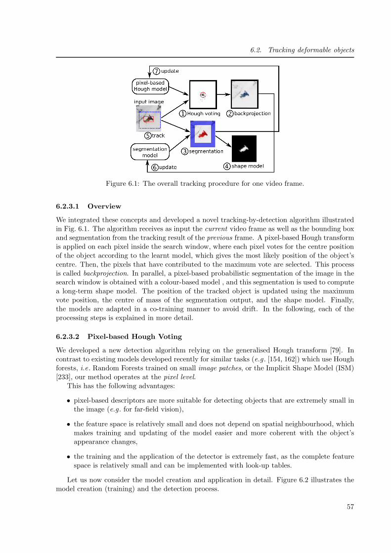
6.2. Tracking deformable objects
Figure 6.1: The overall tracking procedure for one video frame.
6.2.3.1 Overview
We integrated these concepts and developed a novel tracking-by-detection algorithm illustratedin Fig. 6.1. The algorithm receives as input the current video frame as well as the bounding boxand segmentation from the tracking result of the previous frame. A pixel-based Hough transformis applied on each pixel inside the search window, where each pixel votes for the centre positionof the object according to the learnt model, which gives the most likely position of the object’scentre. Then, the pixels that have contributed to the maximum vote are selected. This processis called backprojection. In parallel, a pixel-based probabilistic segmentation of the image in thesearch window is obtained with a colour-based model , and this segmentation is used to computea long-term shape model. The position of the tracked object is updated using the maximumvote position, the centre of mass of the segmentation output, and the shape model. Finally,the models are adapted in a co-training manner to avoid drift. In the following, each of theprocessing steps is explained in more detail.
6.2.3.2 Pixel-based Hough Voting
We developed a new detection algorithm relying on the generalised Hough transform [79]. Incontrast to existing models developed recently for similar tasks (e.g . [154, 162]) which use Houghforests, i.e. Random Forests trained on small image patches, or the Implicit Shape Model (ISM)[233], our method operates at the pixel level.
This has the following advantages:
• pixel-based descriptors are more suitable for detecting objects that are extremely small inthe image (e.g . for far-field vision),
• the feature space is relatively small and does not depend on spatial neighbourhood, whichmakes training and updating of the model easier and more coherent with the object’sappearance changes,
• the training and the application of the detector is extremely fast, as the complete featurespace is relatively small and can be implemented with look-up tables.
Let us now consider the model creation and application in detail. Figure 6.2 illustrates themodel creation (training) and the detection process.
57

Chapter 6. On-line learning of appearance models for tracking arbitrary objects
1st image
trained model
D
Hough voting
voting map
TRAINING DETECTION
Figure 6.2: Training and detection with the pixel-based Hough model. In this example, thered, blue, green, and black pixels belong to the object. Left: in the first frame, the model Dis constructed by storing for each quantised pixel value in the given (red) bounding box all thedisplacement vectors to the object’s centre position (here only colour is used for illustration).Right: in a new frame, the object is detected in a search window by cumulating the displacementvotes of each pixel in a voting map (bright pixels: many votes, dark pixels: few votes).
Training: The detector is trained on the first video frame. Let us denote x = (x1, x2) theposition of a pixel I(x) in an image I. In the training image, the pixels inside a given initialbounding box B0 = (bx0 , b
y0, b
w0 , b
h0) are quantised according to the vector composed of its HSV
colour values and its gradient orientation (see Fig. 6.2 left). This amounts to computing D = Dz
(z = 1..N), an N-dimensional distribution similar to a histogram, which is referred to as pixel-based Hough model in the following. The vectors Dz = d1
z, . . . ,dMzz contain Mz displacement
vectors dmz = (xzm, wzm), each associated with a weight wzm = 1.0. Thus, training consists in
constructing D by traversing each pixel I(x1, x2) inside the bounding box B0, quantising thepixel value as z = zx, computing a displacement vector xz = (bx0 − x1, b
y0 − x2) pointing to the
centre of the bounding box: (bx0 , by0) (illustrated by arrows in Fig. 6.2), and finally adding the
vector dz = (xz, 1.0) to the set Dz.
Detection: in a new video frame, the object can be detected by letting each pixel I(x) insidethe search window vote according to Dz corresponding to its quantised value zx. The right partof Fig. 6.2 illustrates this. Each vote is a list of displacements dm
z that are weighted by wzm
and cumulated in a voting map. The detector’s output is then simply the position in the votingmap with the maximum value xmax.
Backprojection: we can determine how much each pixel inside the search window Ωt con-tributed to the maximum value of the voting map xmax. This process is illustrated in Fig. 6.1and is called backprojection. More precisely, let z be the quantised value of pixel I(x). Then,the backprojection b at each position x ∈ Ωt is defined as:
bx =
wzm if ∃dm
z ∈ Dz s.t. (bx, by) + xzm = xmax ,0 otherwise,
(6.1)
where (bx, by) is the top-left corner of the current bounding box.
58

6.2. Tracking deformable objects
6.2.3.3 Segmentation
Complementary to the local pixel-wise Hough model, a probabilistic soft segmentation approachis adopted, similar to the ones from Aeschliman et al. [60], Cehovin et al. [377] or [312]. Letcx,t ∈ 0, 1 be the class of the pixel at position x at time t: 0 for background, and 1 forforeground, and let yx,0:t be the pixel’s colour observations from time 1 to t. For clarity and aspixels are independent in our approach, we will drop the index x in the following. In order toincorporate the segmentation of the previous video frame at time t−1 and to make the estimationmore robust, we use a recursive Bayesian formulation, where, at time t, each pixel (in the searchwindow) is assigned the probability to belonging to class C ∈ 0, 1 (foreground/background) :
p(ct = 1|y0:t) = Z−1p(yt|ct = 1)∑
c′t−1
p(ct = 1|c′t−1) p(c′t−1|y0:t−1) , (6.2)
where Z is a normalisation constant that makes the probabilities sum up to 1. The distributionsp(yt|ct) are represented with HSV colour histograms. At t = 0, the foreground histogram isinitialised from the pixels in the image region defined by the bounding box around the object inthe first frame. The background histogram is initialised from the image region surrounding thisrectangle. The transition probabilities for foreground and background are set to:
p(ct = 0|ct−1) = 0.6 p(ct = 1|ct−1) = 0.4 . (6.3)
As opposed to recent work on image segmentation (e.g . [324]), we treat each pixel indepen-dently, which, in general, leads to a less regularised solution but at the same time reduces thecomputational complexity considerably.
6.2.3.4 Shape Model
The segmentation gives a rough estimate of the current 2D shape of the tracked object in theimage (see step (3) in Fig. 6.1). We use this estimate to gradually construct a non-parametriclonger-term shape model (step (4) in Fig.6.1), which further helps in the overall tracking, es-pecially for less deforming, i.e. more rigid, objects. The segmentation output is the posteriorprobability of x belonging to the foreground: p(cx,t = 1|yx,0:t). By computing this for all xinside the current search window Ωt, we obtain a 2D segmentation map of the size of Ωt. Theshape sx,t at time t is then recursively estimated as:
sx,t = λφ(p(cx′,t = 1|y0:t)
)+ (1− λ)sx,t−1 ∀x ∈ Ωs , (6.4)
where φ(·) re-samples the segmentation map to a canonical size Ωs = Ω0 (i.e. the initial searchwindow size), and λ = 0.02 is a small update factor. The shape model is initialised at the firstframe with sx,0 = φ
(p(cx′,t = 1|y0)
). It constitutes a scale-invariant discretised representation
of the 2D shape of the object. Figure 6.3 shows illustrations of the automatically learnt objectshape prior models for some of our evaluation videos.
6.2.3.5 Tracking
In a new video frame, pixel-based detection and segmentation are performed inside a searchwindow Ωt, which we set to η = 1.5 times the size of the object’s bounding box. Then, the long-term shape model is updated and the new object’s position Xt = (bxt , b
yt ) and size (bwt , b
ht ) can
be re-estimated. To this end, we utilise not only the output of the detector, i.e. the maximum
59

Chapter 6. On-line learning of appearance models for tracking arbitrary objects
Figure 6.3: Some examples of on-line learnt shape prior models of the videos “ball”, “torus”,“fish2”, “mountainbike”, “trellis”, and “woman”.
position in the voting map, but also the segmentation and shape model, as described in thefollowing. Clearly, this makes the tracking algorithm more robust to non-rigid deformations.
Segmentation map tracking: to infer an estimate of the object’s position from the currentsegmentation, we calculate the centre of mass of the soft segmentation produced by Eq. 6.2:
xs =1
S
∑
x∈Ωt
p(cx = 1|y) x, (6.5)
where S is the sum of all foreground probabilitiesp(cx = 1|y) in the search window Ωt.
Shape correlation: we further exploit the longer-term shape model for tracking the object’sposition by computing the cross-correlation between the shape “map”and the segmentation map(scaled to the same size by φ):
xp = argmaxx
∑
δ∈I
φ(p(cx,t = 1|yx,0:t))sx+δ,t , (6.6)
with I describing the offset in the image, i.e. a discrete 2D displacement of the shape map withinsome reasonable bounds. Thus, we match the current shape model with the segmentation mapin order to obtain a position estimate.
Overall tracking result: At each frame, the new object position is set to a linear combinationof the voting map maximum xmax and the mean of segmentation and shape positions xs andxp:
Xt = (bxt , byt ) = α
xs + xp
2+ (1− α)xmax . (6.7)
The factor α determines how much we trust in the segmentation/shape position compared tothe Hough model’s estimation. It is computed dynamically at each frame by a simple reliabilitymeasure that is defined as the proportion of pixels in the search window Ωt that change fromforeground to background or vice versa, i.e. crossing the threshold p(cx = 1|y) = 0.5.
We further re-estimate the overall scale of the object at each frame using a recursive proba-bilistic inference. See [5] for more details.
6.2.3.6 Model adaptation
Both pixel-based Hough model and segmentation model are updated at each frame in a co-training manner, i.e. the output of one model is used to update the other one. To update theHough model, only foreground pixels are used, that is pixels for which p(cx = 1|y) > 0.5. For
60

6.2. Tracking deformable objects
each of these pixels x the displacement d to the new object’s centre is calculated, and its weightw is set according to its foreground probability:
w ←
γ p(cx = 1|y) + (1− γ)w if d ∈ Dz ,p(cx = 1|y) otherwise,
where γ = 0.1 is the update factor. In the second case (i.e. if d /∈ Dz), d is added to Dz.For computational and memory efficiency, we limit the size of each Dz and only keep the Kdisplacements with the highest weights (K = 20 in our experiments).
The foreground and background distributions of the segmentation model are adapted usingthe backprojection bx. That is, the colour distribution p(y|b > 0.5) of the backprojected pixelsis calculated, and used to linearly update the current foreground colour distribution:
p(yt|ct = 1) = δ p(y|b > 0.5) + (1− δ) p(yt−1|ct−1 = 1) , (6.8)
where δ = 0.1 is the update factor. The background colour distribution is updated in the sameway but using the colour distribution from a rectangular frame surrounding the object borders(as for the initialisation step).
6.2.4 Experiments
We conducted quantitative evaluation on two sets of challenging standard videos that arecommonly used in the literature: the “Babenko sequences” [74]4 and the “Non-rigid objectdataset” [162]5, as well as the public tracking benchmark VOT20146 [218]. The tracking ac-curacy and speed on these datasets has been measured and compared to several state-of-the-arttracking methods.
Using the first two datasets, we compared our algorithm, called PixelTrack+, to 11 state-of-the-art methods: HoughTrack (HT) [162], Tracking-Learning-Detection (TLD) (CVPR ver-sion) [204], Incremental Visual Tracker (IVT) [323], the Multiple Instance Learning tracker(MIL) (CVPR version) [74], the ℓ1 tracker using the Accelerated Proximal Gradient method (ℓ1APG) [80], the structured output tracker: Struck (ICCV version) [175], Multi-Level Quantisa-tion tracker (MQT) [191], the Deep Learning Tracker (DLT) [391], MEEM [430], DSST [127]and MUSTer [192].
To measure the performance of the different tracking algorithms, we determine, for eachvideo, the proportion of frames in which the object is correctly tracked. And, to measure thetracking precision, we computed the average Normalised Centre Error (NCE) on each video,i.e. the Euclidean distance between the ground truth rectangle’s centre and the correspondingtracked bounding box in a frame. Table 6.1 summarises the results. Although our method is notdesigned for grey-scale videos and, thus, does not show its full potential, it still performs betteron average than most of the state-of-the-art methods. Only MEEM outperforms PixelTrack+on both measures. DSST and MUSTer also generally have a higher proportion of successfullytracked frames as they rely less on colour segmentation which is not useful in grey-scale videos.
For the VOT2014 data, we followed the evaluation protocol of the benchmark [219], usingthe accuracy (same as our correctly tracked frame measure above) and the robustness (numberof tracking failures). Figure 6.4 shows the accuracy-robustness plots for the baseline experimentof the VOT2014 benchmark [218] comparing 33 state-of-the-art tracking methods. Our method
4http://vision.ucsd.edu/ bbabenko/project miltrack.html5http://lrs.icg.tugraz.at/research/houghtrack/6http://votchallenge.net/
61
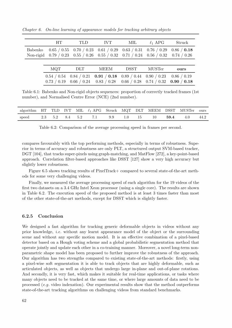
Chapter 6. On-line learning of appearance models for tracking arbitrary objects
HT TLD IVT MIL ℓ1 APG Struck
Babenko 0.65 / 0.55 0.70 / 0.23 0.61 / 0.29 0.63 / 0.31 0.76 / 0.29 0.86 / 0.18Non-rigid 0.79 / 0.23 0.55 / 0.26 0.55 / 0.32 0.71 / 0.24 0.56 / 0.32 0.74 / 0.26
MQT DLT MEEM DSST MUSTer ours
0.54 / 0.54 0.84 / 0.21 0.91 / 0.18 0.89 / 0.44 0.90 / 0.23 0.86 / 0.190.73 / 0.19 0.66 / 0.24 0.83 / 0.28 0.66 / 0.28 0.74 / 0.32 0.90 / 0.18
Table 6.1: Babenko and Non-rigid objects sequences: proportion of correctly tracked frames (1stnumber), and Normalised Centre Error (NCE) (2nd number).
algorithm HT TLD IVT MIL ℓ1 APG Struck MQT DLT MEEM DSST MUSTer ours
speed 2.3 5.2 8.4 5.2 7.1 9.9 1.0 15 10 59.4 4.0 44.2
Table 6.2: Comparison of the average processing speed in frames per second.
compares favourably with the top performing methods, especially in terms of robustness. Supe-rior in terms of accuracy and robustness are only PLT, a structured output SVM-based tracker,DGT [104], that tracks super-pixels using graph-matching, and MatFlow [272], a key-point-basedapproach. Correlation filter-based approaches like DSST [127] show a very high accuracy butslightly lower robustness.
Figure 6.5 shows tracking results of PixelTrack+ compared to several state-of-the-art meth-ods for some very challenging videos.
Finally, we measured the average processing speed of each algorithm for the 19 videos of thefirst two datasets on a 3.4 GHz Intel Xeon processor (using a single core). The results are shownin Table 6.2. The execution speed of the proposed method is at least 3 times faster than mostof the other state-of-the-art methods, except for DSST which is slightly faster.
6.2.5 Conclusion
We designed a fast algorithm for tracking generic deformable objects in videos without anyprior knowledge, i.e. without any learnt appearance model of the object or the surroundingscene and without any specific motion model. It is an effective combination of a pixel-baseddetector based on a Hough voting scheme and a global probabilistic segmentation method thatoperate jointly and update each other in a co-training manner. Moreover, a novel long-term non-parametric shape model has been proposed to further improve the robustness of the approach.Our algorithm has two strengths compared to existing state-of-the-art methods: firstly, usinga pixel-wise soft segmentation it is able to track objects that are highly deformable, such asarticulated objects, as well as objects that undergo large in-plane and out-of-plane rotations.And secondly, it is very fast, which makes it suitable for real-time applications, or tasks wheremany objects need to be tracked at the same time, or where large amounts of data need to beprocessed (e.g . video indexation). Our experimental results show that the method outperformsstate-of-the-art tracking algorithms on challenging videos from standard benchmarks.
62

6.2. Tracking deformable objects
51015202530
5
10
15
20
25
30
Robustness rank
Acc
urac
y ra
nk
Ranking plot for experiment baseline
0 0.2 0.4 0.6 0.8 10
0.2
0.4
0.6
0.8
1
Robustness (S = 30.00)A
ccur
acy
AR plot for experiment baseline
ABS ACT CT DSST eASMS FoT FSDTIIVTv2 IPRT KCF LT_FLO MIL OGT PLT_14qwsEDFT SIR_PF VTDMG ACAT aStruck CMT DGTDynMS EDFT FRT HMMTxD IMPNCC IVT LGTv1MatFlow NCC PLT_13 SAMF Struck PTp
Figure 6.4: Comparison with 33 state-of-the-art methods of the VOT2014 benchmark [218]. Theproposed method “PTp” is among the top-performing methods with the fifth-best robustness.
DLT MEEM DSST MUSTer PixelTrack+
Figure 6.5: Tracking results of DLT [391], MEEM [430], DSST [127], MUSTer [192] and theproposed PixelTrack+ on some of the more challenging videos from the non-rigid object datasetand the VOT2014 benchmark (best viewed in colour).
63
Chapter 6. On-line learning of appearance models for tracking arbitrary objects
6.3 On-line learning of motion context
6.3.1 Introduction
As experimental results show, the previous work addressed well the problem of tracker driftand is able to learn on-line a stable appearance model in dynamic environments. However,when analysing the behaviour and the results of our tracking algorithms and the ones from theliterature, we realised that there are still certain failure modes, e.g . certain situations that havenot been considered in the design of these algorithms. One of these situations is when, in thebackground, there are very similar objects to the one(s) that we want to track, and when oneor several of these distracting objects comes close to it. Then many algorithms might lose trackand “jump” to the image region corresponding to the most similar object. This happens, forinstance, when tracking a person in sports videos or an animal in a herd or swarm. Thus, ina SOT problem, it seems important to not only consider the object to track but also its globalenvironment.
For this reason, together with Christophe Garcia, we studied methods to incorporate thecontext of the visual scene into the tracking process. In many practical applications, the camerais moving. Thus, the background and the visual context is also changing over time. Therefore,we adopted again an on-line learning approach in order to be able to dynamically adapt tonew environments and situations. In contrast to the tracking-by-detection method PixelTrack+described in the previous section, we opted here for a probabilistic Bayesian approach, as itallows for a straightforward integration and combination of different appearance models andobservation likelihoods as well as motion models, and for an effective inference with particlefiltering.
6.3.2 State of the art
One of the first works to explicitly include context in visual object tracking has been the Context-Aware Tracker (CAT) by Yang et al . [414]. Their method operates on-line throughout the videoand continuously discovers objects that move in the same direction as the tracked object byperforming a motion correlation analysis. These auxiliary objects help to support and improvetracking by performing inference in a star-structured graphical model that includes the objects’states. Similarly, Zhang et al . [431] modelled the spatio-temporal relationships and correlationsbetween the object and its locally dense contexts in a Bayesian framework.
Spatial context has also been exploited by using supporters, i.e. other objects or featurepoints around the target in the image. For example, this may be useful in videos, where a handholds the object to track and thus exhibits the same visible motion pattern. Or when groups ofpeople walk in the same direction. Grabner et al . [167], for example, extended the well-knownImplicit Shape Model by detecting feature points in the image that have a correlated motion withthe target. These supporters are matched from frame to frame, and their relative displacementvectors are updated on-line. Wen et al . [399] also proposed a method that detects supporters(here called contributors) which are interest points within a local neighbourhood around thetarget, in order to improve the tracking performance. In addition, their method makes use of alonger-term temporal context using an on-line sub-space learning method that groups togetherobservations from several frames. Similarly, the approach proposed by Sun et al . [362] tracks“helper”objects using an on-line Adaboost detector, initialised manually at the first frame. Theirrelative position is learnt on-line and used to predict the target object’s position.
Dinh et al . [136] proposed a method using supporters as well as distractors, which are objectswith similar appearance to the target. The distractors help to avoid confusion of the tracker with
64

6.3. On-line learning of motion context
other similar objects in the scene, and they can possibly be used to reason about the objects’mutual occlusion. In the work of Dinh et al ., supporters are not used directly for the target’sstate estimation but only to disambiguate between the target and its distractors. Hong etal . [190] recently proposed an approach based on the ℓ1 tracker [277] that deals with distractorsby automatically learning a metric not only between positive and negative examples but alsowithin the collected negative examples, effectively replacing the originally proposed Euclideandistance. Finally, Supancic and Ramanan [363] presented a self-paced learning tracker that alsoselects training examples from video frames in the past to perform long-term tracking, an ideathat has also been used in the recent work of Hua et al . [195].
The disadvantage with using supporting and distracting objects is that several objects needto be detected and tracked, which can be computationally expensive especially with a largernumber of objects. Moreover, the success or failure of data association or, in some methods,matching local features points in successive video frames, heavily depends on the type of object totrack and the surrounding background. This process can be error-prone and, in some situations,may rather harm the overall tracking performance. Finally, modelling the spatial, temporal, orappearance-based pairwise relationships between objects and/or interest points can lead to acombinatorial explosion and make the inference on the state space difficult.
To alleviate this problem, in this work, we propose a probabilistic method that dynamicallyupdates the foreground and background model depending on distracting objects or image regionsin the scene background. This contextual appearance information is extracted from movingimage regions and used to train on-line a discriminative binary classifier that, in each videoframe, detects the image region corresponding to the object to track.
Traditionally, these discriminative on-line classifiers used in tracking-by-detection approaches[74, 154, 162, 165, 175, 277] learn negative examples extracted from the image region surroundingthe current target object region. This choice is motivated by the fact that the object willmove only slightly from one frame to the other w.r.t. the background or other objects, and bycomputational speed. In contrast, our method uses a stochastic sampling process to extractnegative examples from image regions that move. We call these: contextual motion cues (seeFig. 6.6). In that way, regions that correspond to possibly distracting objects are detectedefficiently and early, i.e. without them having to be inside a search window and without scanningthe whole image at each point in time.
6.3.3 Tracking framework with discriminative classifier
In this work, we used a traditional recursive Bayesian model for tracking and a particle filter,i.e. sampling importance resampling (SIR) or bootstrapping, for the inference [139, 198]. Aswe already described the principal model before (c.f . section 5.2.3 for MOT and section 5.3.3for SOT), we only concentrate on the original parts and on our contributions, i.e. the on-linelearning of a discriminative classifier using motion context cues and its integration in the particlefilter framework using an effective likelihood model and proposal functions.
6.3.3.1 Object state representation and inference
The state X = (x, y, vx, vy, s, e) ∈ R6 of the object to track is described by an upright bounding
box defined by the object’s centre position (x, y) in the image, its 2D speed (vx, vy) in the imageplane, scale (s), and eccentricity (e), i.e. the ratio of height and width. The state X0 is initialisedmanually by providing a bounding box around the object in the first frame. Then, for each videoframe, the particle filter performs its classical steps of predicting particles X(i) sampled from
65
Chapter 6. On-line learning of appearance models for tracking arbitrary objects
the proposal distribution q(Xt|Xt−1) and updating their weights according to the observationlikelihood p(Yt|Xt), state dynamics pm(Xt|Xt−1) and proposal (see Section 6.3.3.2): wi =
p(Yt|Xt)pm(Xt|Xt−1)q(Xt|Xt−1)
, for each particle i ∈ 1..N . At the end of each iteration, the observation
likelihood model parameters are updated using the mean of the posterior distribution p(Xx|Y1:t).And finally, systematic resampling is performed.
6.3.3.2 State dynamics and proposal function
In order to cope with fairly complex motion of arbitrary objects in videos from a possibly movingcamera, we used a proposal function composed of a mixture of three distributions:
q(Xt|Xt−1) = βmpm(Xt|Xt−1)
+ βfpf (Xt|Xt−1)
+ βdpd(Xt|Xt−1) ,
(6.9)
where βm, βf , βd < 1 define the mixture weights (∑
i βi = 1), and pm(Xt|Xt−1) is the statedynamics model (similar to the ones in sections 5.2.3.2 and 5.3.3), pf (Xt|Xt−1) is an opticalflow-like motion-based proposal function, and pd(Xt|Xt−1) proposes states coming from a dis-criminative on-line trained detector described in more detail in section 6.3.4.
6.3.3.3 Observation likelihood
The observation likelihood function p(Y|X) that we proposed is designed to be robust againstobject deformations, pose and illumination changes as well as partial occlusions. It is a geometricmean of three distributions corresponding to different visual cues:
p(Yt|Xt) = (pH(Yt|Xt) pS(Yt|Xt) pT (Yt|Xt))1/3 , (6.10)
where pH computes a local colour histogram likelihood ratio, pS measures the global colourdistribution similarity, and pT is a texture likelihood based on the on-line learnt discriminativeclassifier that we will explain in the following section. Taking the cube root of the productensures that the overall likelihood distribution does not become too peaked. For more details,refer to [6].
6.3.4 Model adaptation with contextual cues
In this section, we will describe the main contribution of the proposed approach: a method toexploit motion context effectively for visual object tracking using a discriminative classifier thatis trained on-line on specific parts of the input video. Our approach is different from previouswork, where motion context or background motion has been integrated tightly in the trackingprocess (e.g . in [160, 293], or where specific appearance models are used to avoid distractions inthe background [136, 190].
In our particle filter framework outlined above, we used a binary discriminative classifierbased on the On-line Adaboost (OAB) algorithm [165] (based on Haar-like features) for proposingnew particles as well as for evaluating the observation likelihood. Any other on-line classifiercould have been used as well. The classifier is trained with the first video frame using the imagepatch inside the object’s bounding box as a positive example and surrounding patches within asearch window as negative examples (as we cannot infer motion from a single image). Then, theclassifier is updated at each tracking iteration using the same strategy for extracting positiveand negative examples. We refer to [165] for details on the model and how it is trained.
66

6.3. On-line learning of motion context
Figure 6.6: Illustration of different sampling strategies of negative examples (blue). Left: tradi-tional sampling at fixed positions within a search window (red). Middle: the motion probabilitydensity function m (Eq. 6.11). Right: the proposed negative sampling from m.
6.3.4.1 Background sampling
We propose to sample negative examples from image regions that contain motion and thus likelycorrespond to moving objects (see Fig. 6.6). The idea is that these regions may distract thetracker at some point in time. Therefore, it is preferable to incorporate these distracting imageregions in the classifier training in the form of negative examples and learn them as early aspossible, i.e. as soon as they appear in the scene. One can see this as a kind of long-termprediction of possible negative samples, in contrast to the much shorter (frame-by-frame) timescale of the proposal function. To perform this negative sampling, we first compensate for cameramotion between two consecutive frames using a classical parametric motion estimation approach[292]. We apply a three-parameter model to estimate the translation and scale factor betweenthe images, and then compute the intensity differences for each pixel in the current image withits corresponding pixel in the previous frame. This gives an image M(x, y) approximating theamount of motion present at each position (x, y) of the current frame of the video. We thentransform this image into a probability density function (PDF) m(x, y) over the 2-dimensionalimage space:
m(x, y) = Z−1∑
(u,v)∈Ω(x,y)
M(u, v) , (6.11)
where Ω(x, y) defines an image region of the size of the bounding box of the object being tracked,centred at (x, y), and Z is a constant normalising the density function to sum up to 1. Thus,m(x, y) represents the relative amount of motion inside the region centred at (x, y). Finally, N−
image positions (x, y) are sampled from this PDF corresponding to rectangles centred at (x, y).That is, statistically, regions with high amount of motion are sampled more often than staticimage regions. This process is illustrated in Fig. 6.6.
6.3.4.2 Classifier update
The N− image patches corresponding to the sampled regions as well as the positive examplecoming from the mean particle of the tracker are then used to update the classifier. In this case,the OAB method needs a balanced number of positives and negatives, thus the positive exampleis used N− times, alternating positive and negative updates.
The advantage of sampling positions from these motion cues is that we do not need to careabout explicitly detecting, initialising, tracking, and eventually removing a certain number ofdistracting objects at each point in time. Note that we could also sample regions of differentscales but as scale does not change rapidly in most videos the benefit of this is relatively small.
67

Chapter 6. On-line learning of appearance models for tracking arbitrary objects
fixed fixed+random motion fixed+motion
Babenko 73.28 74.06 82.30 85.25Non-rigid 68.71 70.30 74.29 80.87
Table 6.3: Average percentage of correctly tracked frames with the proposed method usingdifferent negative sampling strategies.
Note also that the PDF could as well include appearance similarity with the tracked target.However, this would considerably increase the computational complexity.
6.3.5 Experiments
We performed a quantitative evaluation of our proposed approach, that we called “Motion Con-text Tracker” (MCT), on four challenging public tracking datasets: the Babenko and Non-rigidobject sequences also used to evaluate our PixelTrack+ method, described in the previous sec-tion, and the VOT2013 and the VOT2014 datasets. Again, we measured the accuracy (≡ thepercentage of correctly tracked frames) and the robustness (≡ number of tracking failures).
In the first experiments, we evaluated different strategies for the collection of negative ex-amples of the discriminative OAB classifier, as explained in Section 6.3.4. We compared fourdifferent strategies:
• fixed: N− negatives are taken from fixed positions around the positive example inside thesearch window, which is twice the size of the object’s bounding box.
• fixed+random: N−/2 examples are taken from fixed position (as for “fixed”), and N−/2examples are sampled from random image positions.
• motion: N− negative examples are sampled from the contextual motion distribution m(Eq. 6.11).
• fixed+motion: N−/2 examples are taken from fixed positions, and N−/2 examples aresampled from the contextual motion distribution.
In any case, the negative examples do not overlap more than 70% with the positive ones inthe image. Table 6.3 shows the results for the first two datasets in terms of the percentageof correctly tracked frames. On average, the best strategy is “fixed+motion”, with a relativeimprovement of around 7.5%.
Using the VOT2013 benchmark, we compared MCT with 27 other state-of-the-art trackingmethods. Table 6.4 lists the top 7 ranks for the experiments baseline, region-noise (i.e. withperturbed initial bounding boxes), and greyscale (i.e. videos converted to grey-scale), combiningaccuracy and robustness. The results of MCT are very competitive, being the second-bestmethod for baseline and region-noise and the third-best for greyscale. We also added the methodPF (MCT without the detector) to the VOT2013 evaluation. Its overall ranks for the baseline,region-noise, and greyscale experiments are 16.1, 14.5, and 14.4 respectively. This clearly showsthat the benefit of the motion context-based discriminative classifier.
Finally, Table 6.5 lists the 10 best methods for VOT2014 and the respective accuracy ranks,robustness ranks, and overall ranks. Overall, the results of our MCT approach are very compet-itive. Taking the average of accuracy and robustness ranks, PLT and its extension PLT 14 arestill slightly better, as well as the correlation filter-based method SAMF [413], and the method
68

6.3. On-line learning of motion context
baseline region-noise greyscale
PLT 4.96 PLT 3.58 PLT 3.96MCT 6.62 MCT 5.08 FoT [384] 4.75FoT [384] 8.25 CCMS 8.33 MCT 6.25EDFT [146] 9.5 FoT [384] 9.04 EDFT [146] 7.5CCMS 9.54 LGT++ [408] 9.04 GSDT [155] 9.5LGT++ [408] 10.2 EDFT [146] 9.08 LGT++ [408] 9.58DFT [336] 11.1 LGT [377] 10.5 Matrioska [272] 10.7
Table 6.4: Overall ranking result with the VOT2013 dataset. Only the first 7 out of 28 ranksare shown.
accuracy rank robustness rank overall rank
SAMF [413] 8.16 16.49 12.33PLT 14.28 10.41 12.35DGT [104] 11.42 13.44 12.43PLT 14 17.46 10.77 14.12MCT 13.52 14.76 14.14PF 13.70 14.74 14.22DSST [127] 13.51 15.54 14.53KCF [182] 13.62 16.82 15.22HMMTxD [218] 13.18 17.57 15.38MatFlow [272] 16.90 15.29 16.10
Table 6.5: Overall ranking result with the VOT2014 dataset. Only the first 10 out of 39 ranksare shown.
DGT [104] which relies on graph matching and super-pixel representations. The method PF,i.e. MCT without the discriminative classifier, is only slightly worse on average with this bench-mark. This might be due to the more challenging type of videos with deformable objects forwhich the texture-based classifier is not powerful enough.
In terms of execution speed, our algorithm runs at around 20fps for a frame size of 320×240on an Intel Xeon 3.4GHz (single core).
6.3.6 Conclusion
We proposed a new efficient particle filter-based approach for tracking arbitrary objects in videos.The method combines generative and discriminative models, by effectively integrating an on-line learning classifier. We introduced a new method to train this classifier that samples theposition of negative examples from contextual motion cues instead of a fixed region aroundthe tracked object. Our extensive experimental results show that this procedure improves theoverall tracking performance with different discriminative classification algorithms. Further, theproposed tracking algorithm gives state-of-the-art results on four different challenging trackingdatasets, effectively dealing with large object shape and appearance changes, as well as complexmotion, varying illumination conditions and partial occlusions. Note that we also officiallyparticipated in the VOT2014 challenge [32] and the associated workshop held in conjunction
69

Chapter 6. On-line learning of appearance models for tracking arbitrary objects
with ECCV 2014 [31]. As can be seen from the results (c.f . 6.5), our MCT method achieved anexcellent position in the ranking.
In summary, we have shown experimentally that dynamically integrating context informationfrom the visual scene using on-line learning can largely improve the overall performance of thetracking algorithm. In the following section, we will outline our research work that develops thisidea further by constructing finer global scene context models in an on-line manner.
6.4 Dynamic adaptation to scene context
6.4.1 Introduction
In this section, I will present our research work performed in the context of the PhD thesis ofSalma Moujtahid [23, 28, 29, 283]. We worked on another approach of including contextualscene or background information in the tracking process, and we applied it to the SOT scenario,as in the previous section. However, here, scene context is not used for the on-line learning ofrobust appearance models, as with MCT, but for a dynamic selection of trackers among a set ofmethods depending on their suitability for the given environment at each point in time.
Many tracking algorithms have been proposed in the literature, and each of them hasstrengths and weaknesses depending on the appearance, motion or state models or the typeof inference.
Our assumption was that their performance varies in different types of settings and environ-ments and, thus, for a given context, we would be able to select the algorithm and model that ismost appropriate. As these variations might occur not only from one type of video or applicationto another but also within a given video stream, we developed a method that dynamically selectsone tracker from a pool of supposedly complementary trackers depending on the scene contextat a given point in time. To this end, we conceived a set of general scene context features,and we extracted these features from each frame of a set of training videos. Then, a classifierwas trained (off-line) on these features to predict which tracker is the most suitable for a givenmoment in the video. Finally, we proposed an original tracking framework that selects the mostappropriate tracker at each frame based on this classifier. In the following, we will describe thisapproach in more detail.
6.4.2 State of the art
Many ways of combining, fusing or selecting visual models or features for tracking exist in theliterature. They can be categorised into low-level and high-level fusion approaches.
6.4.2.1 Low-level fusion
Fusion at a low level means the combination of multiple visual features in a single trackingmodel. Early works like the one from Birchfield et al . [95] used the sum of colour histogramsand intensity gradient likelihoods. Collins et al . [122] also used likelihood maps to rank featuresand select the most discriminant ones. Triesh et al . [369] weight features in other to fuse themin a democratic integration for face tracking. A Bayesian framework introduced by Yilmazet al . [422] fuses probabilistic density functions based on texture and colour features for objectcontour tracking. Other existing works (e.g . [305, 349, 423]) fuse different modalities, like motionor shape, in order to improve the overall foreground-background discrimination. The low-levelfusion of features might lead to problems because of the interdependence of the features in the
70

6.4. Dynamic adaptation to scene context
tracking model. If some of the visual cues are altered or occluded because of changing sceneconditions, the whole model is prone to drift.
6.4.2.2 High-level fusion
Other approaches consider the combination of the output of multiple trackers. For example,a probabilistic combination was proposed by Leichter et al . [234] with multiple synchronoustrackers using different features where each tracker estimates a probability density function ofthe tracked state. A sampling framework is introduced by Kwon et al . [222, 223] integratingestimates from basic complementary trackers using different observation models and motionmodels. Moreover, tracker performance within a parallel framework can be measured as thedisagreement of a tracker with respect to the other trackers. Li et al . [244] exploited this ideato seek a balance between the trackers. The recent work by Khalid et al . [212] fuses the outputof multiple trackers based on their estimated individual performance and the spatio-temporalrelationships of their results. Using the object trajectory as a fusion criteria is another possibility.For example, Bailer et al . [76] used trajectory optimisation to fuse the tracking results (boundingboxes) from different tracking algorithms. Wang et al . [392] also modelled the object trajectoryand the reliability of each of five independent trackers combining them with a factorial HiddenMarkov Model (HMM). More recently, Vojir et al . [383] also utilised a HMM to fuse observationsfrom complementary trackers and a detector. The HMM’s latent states correspond to a binaryvector expressing the failure of the individual trackers.
In a different manner, rather than using multiple trackers with different cues, Zhang etal . [430] retain snapshots of a base tracker (an on-line SVM) in time, constituting an ensembleof its past models. Then a model is restored according to an entropy criterion.
In terms of tracker selection rather than fusion, our previous work [29] presented a simpleselection framework using the trackers confidences and a spatio-temporal criteria. SimilarlyStenger et al . [351] also used confidences to select the best tracker applied to face tracking. Themain advantage of selection algorithms is that the resulting tracking output is not altered byone or more trackers that may have drifted as long as they are not selected.
In contrast to these fusion frameworks, our proposed selection framework does not rely solelyon the performance or tracking results of our trackers. It differs essentially in the use of the scenecontext in the decision of selecting the most suitable tracker at each point in time. Moreover,selecting from a pool of independent trackers allows to adapt to rapid scene changes and quicklyswitch between different models.
6.4.2.3 Context in tracking
Scene context has been used previously in visual tracking and detection. Especially in on-line detection or tracking scenarios, where information for model construction is very limitedto the number of frames, context can provide important information and greatly improve theperformance. Context can be used in many ways. As mentioned in section 6.3.2, some works(e.g . [167, 399, 414, 431]) use “supporters”, i.e. image regions or interest points moving similarlyto the tracked object and assisting the tracking, or “distractors” [136, 190], i.e. image regionswith similar appearance to the object, in order to avoid confusion in tracking. However, themodelling of spatial and temporal relationships between the different tracked objects or interestpoints is computationally expensive, due to the more complex data association. In a differentmanner, Maggio et al . [270] used contextual event cues such as target births (objects enteringthe scene) and spatial clutter of objects. The spatial distribution of these events is incrementally
71
Chapter 6. On-line learning of appearance models for tracking arbitrary objects
learned using tracker feedback for MOT.
In our approach, supporters, distractors or contextual events are not used because they makeinference more complex and error-prone due to detection or tracking errors. We rather classifythe general scene context and conditions in order to select the most appropriate visual cue ortracker for a given situation. To this end, we compute global image descriptors based on colour,intensity and motion at each video frame. In the past, other global image descriptors (sometimescalled gist features) have been proposed (e.g . [298, 341, 367]) mostly for fixed images to classifyscenes into different semantic categories, such as open, closed environments, indoor, outdoor etc.
6.4.3 Visual scene context description
One of our main goals is to globally characterise the scene at a given point in time throughdescriptors extracted from the image. For instance, we want to capture if the overall environmentis rather dark or light, if it is cluttered, if the motion in the background is homogeneous etc. Wealso need to correlate these descriptors with the features used in the individual trackers fromour pool of trackers Tn, (n ∈ 1..N). We thus designed descriptors, called “scene features”, basedon first and second order statistics of the main image characteristics (e.g . intensity, hue, motionvectors). We defined these low-level features such that they can be easily interpreted, and, atthe same time, help the process of learning and correlating a scene condition to a tracker.
Using Equations 6.12-6.15, we define our scene features fΩk over an image region Ω as:
Intensity and texture features:
- Average brightness (fΩ1 ): the mean grey-scale pixel value (see Eq. 6.12).
- Average contrast (fΩ2 ): the mean squared value of the difference of each grey-scale pixel
and the average brightness (see Eq. 6.15).
Chromatic features:
- Average saturation (fΩ3 ): the mean pixel value of the saturation channel in HSV colour
space (Eq. 6.12).
- Saturation variance (fΩ4 ): the variance of saturation (Eq. 6.13).
- Dominant hue (fΩ5 ): the dominant colour extracted from a histogram of quantised hue
pixel values in HSV colour space (Eq. 6.14).
- Hue variance (fΩ6 ): the variance of the pixel values in the hue channel (Eq. 6.13).
Motion features:
- Average motion (fΩ7 ): the mean of the norm of optical flow vectors (Eq. 6.12).
- Motion variance (fΩ8 ): the variance of the norm of dense optical flow vectors (Eq. 6.13).
Let pi denote the pixel value of a given image channel (e.g . H,S,V) and ‖Ω‖ the number ofpixels in the region Ω. The above mentioned features are then defined as follows:
72

6.4. Dynamic adaptation to scene context
Local region
Global region
Differential region
Figure 6.7: The different image regions used to compute scene features.
average: fΩk =
∑i∈Ω pi
‖Ω‖ , for k = 1, 3, 7 (6.12)
variance: fΩk =
∑i∈Ω(pi)
2
‖Ω‖ −(∑
i∈Ω pi
‖Ω‖
)2
, for k = 4, 6, 8 (6.13)
dominant cue: fΩk = argmax
i∈Ω(pi), for k = 5 (6.14)
contrast: fΩk =
1
‖Ω‖∑
i∈Ω
(pi −
∑i∈Ω pi
‖Ω‖
)2
, for k = 2. (6.15)
Each of these features k is computed on three different image regions Ω as shown in Fig.6.7.We define a global value as the feature computed on the whole image: fG
k . The local valueis the feature computed on the Region Of Interest (ROI): fL
k . And a differential value asthe difference between the feature computed on the foreground region (i.e. the ROI) and thebackground region (i.e. the image not including the ROI): fD
k .Not every combination of feature and region is used as some of them have little semantic meaning.The concatenation of these features gives us:
fG =fG1 , . . . , fG
3 , fG6 , . . . , fG
8
, (6.16)
fL =fL1 , . . . , f
L8
,
fD =fD1 , . . . , fD
7
.
Finally, we obtain M = 21 scene context features ft =fGt , fLt , f
Dt
for frame t.
6.4.4 A scene context-based tracking approach
6.4.4.1 Supervised learning of scene context
The scene context classifier’s goal is to learn the different patterns that show high correlationbetween the information extracted from the scene context (described by our scene features) andthe performance of a tracker in the particular set of conditions. As multi-class classifier, we chosea fully connected Multi-Layer Perceptron (MLP) with one hidden layer, N output neurons andsigmoid activation functions. Any other algorithm could be used as well. In fact, a multi-classSVM showed equivalent performance in our experiments.
As shown in Fig.6.8, the classifier’s input it at a frame t consists of several components: Thescene features ft extracted from the scene characterise the scene, the confidence values of the
73
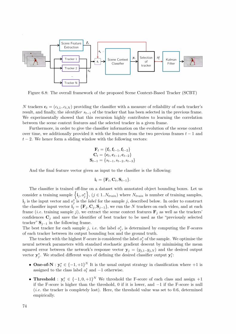
Chapter 6. On-line learning of appearance models for tracking arbitrary objects
Tracker 1
Tracker 2
Tracker N
Scene Feature
Extraction
Kalman
Filter
Scene Context
Classifier
Selection
of
tracker
Figure 6.8: The overall framework of the proposed Scene Context-Based Tracker (SCBT)
N trackers ct = (ct,1..ct,N ) providing the classifier with a measure of reliability of each tracker’sresult, and finally, the identifier st−1 of the tracker that has been selected in the previous frame.We experimentally showed that this recursion highly contributes to learning the correlationbetween the scene context features and the selected tracker in a given frame.
Furthermore, in order to give the classifier information on the evolution of the scene contextover time, we additionally provided it with the features from the two previous frames t− 1 andt− 2. We hence form a sliding window with the following vectors:
Ft = ft, ft−1, ft−2Ct = ct, ct−1, ct−2
St−1 = st−1, st−2, st−3
And the final feature vector given as input to the classifier is the following:
it = Ft,Ct,St−1.
The classifier is trained off-line on a dataset with annotated object bounding boxes. Let us
consider a training sampleij , o
∗j
, (j ∈ 1..Ntrain) where Ntrain is number of training samples,
ij is the input vector and o∗j is the label for the sample j, described below. In order to constructthe classifier input vector ij = Fj,Cj ,Sj−1, we run the N trackers on each video, and at eachframe (i.e. training sample j), we extract the scene context features Fj as well as the trackers’confidences Cj and save the identifier of best tracker to be used as the “previously selectedtracker” Sj−1 in the following frame.The best tracker for each sample j, i.e. the label o∗j , is determined by computing the F-scoresof each tracker between its output bounding box and the ground truth.
The tracker with the highest F-score is considered the label o∗j of the sample. We optimise theneural network parameters with standard stochastic gradient descent by minimising the meansquared error between the network’s response vector yj = (yj,1..yj,N) and the desired outputvector y∗
j . We studied different ways of defining the desired classifier output y∗t :
• One-of-N : y∗t ∈ −1,+1N It is the usual output strategy in classification where +1 is
assigned to the class label o∗t and −1 otherwise.
• Threshold : y∗t ∈ −1, 0,+1N We threshold the F-score of each class and assign +1
if the F-score is higher than the threshold, 0 if it is lower, and −1 if the F-score is null(i.e. the tracker is completely lost). Here, the threshold value was set to 0.6, determinedempirically.
74

6.4. Dynamic adaptation to scene context
• Ranking : y∗t ∈ −1,−0.3,+0.3,+1N We rank the F-scores of our classes, and assign
respectively +1, +0.3 and −0.3 from highest to lowest F-score. If the F-score value is 0,than −1 is assigned to the corresponding class.
• Regression : y∗t = Fscore1t , .., FscoreNt We directly use the F-score values, so the
classifier trains to predict these values.
The network’s final class prediction, i.e. the predicted best tracker index, is simply oj =argmaxn∈N yj,n.
6.4.4.2 On-line tracker selection and learning
The proposed algorithm uses N independent on-line trackers that are initialised with the bound-ing box of the object in the first video frame. Then, as illustrated in Fig. 6.8, the trackers andthe context feature extraction operate in parallel providing at each frame N confidence valuesCt and M scene context features Ft respectively. At each video frame t, the scene context clas-sifier estimates a score for each tracker yt to perform best under the current scene context. Weselect the tracker with the highest score as the most suitable tracker st = argmaxn∈N yt,n. Thebounding box Bs
t from the selected tracker T st is then passed to a Kalman Filter to deal with
imprecise estimations and to provide a smoother object trajectory. Finally, the last step is thegeneral update of the trackers with the filtered bounding box. The individual trackers train theirmodels on-line. They use the ground truth bounding box of the first frame to initialise theirmodels and update them every frame once a prediction is made using the selected bounding boxBs
t processed by the Kalman filter.
6.4.5 Experiments
To evaluate our proposed approach we used a set of three trackers based on the Kernelized Cor-relation Filter (KCF) [182] and with three different types of complementary features: Histogramof Oriented Gradients (HOG), raw grey-scale intensities and quantised colours in the CIE-labcolour space. Note that our proposed method is completely independent of the underlyingindividual tracking algorithms.
We evaluated first the performance of the proposed scene context classifier based on the scenecontext features. To train the classifier we used the Princeton Tracking Benchmark Dataset [348],containing 100 videos, and a section of the ILSVRC2015 Dataset [325]. With a total of 397 videos(106 203 training samples and 12 700 validation samples), the dataset represents a diverse set ofobject types, background and scene conditions. For testing, we used the dataset of the VOT2013benchmark [217]. The input features have been computed with the tracking output of the threeKCF trackers. Table 6.6 shows the classification results for the different strategies for the outputvalue y∗
t . One can see the that, the classifier is able to predict the best tracker in around 80% ofthe video frames. The One-of-N training strategy gives the best result and Ranking the secondbest. The table shows also the overall tracking results of the proposed framework. Here, theRanking strategy gives considerably better results.
Table 6.7 shows more detailed tracking results on VOT2013. The proposed tracker selectionframework improves both accuracy and failure rate (robustness) compared to the individualtrackers. Also the Kalman Filter and the general update, i.e. updating the individual modelsonly using the bounding box of the selected tracker, increase the overall performance. Moreresults as well as a comparison with the state-of-the-art can be found in [28].
75

Chapter 6. On-line learning of appearance models for tracking arbitrary objects
Classifier output y∗t Train rate Test rate Accuracy Failures
One-of-N 89.56 % 79.56 % 0.583 1.313
Threshold 63.77 % 51.76 % 0,600 1,440
Ranking 88.95 % 77.82 % 0.607 0.563
Regression 69.80 % 62.24 % 0,590 1,130
Table 6.6: Correct classification rates on training (Princeton + ILSVRC15) and test (VOT2013)datasets for context classifiers trained using different desired output y∗
t strategies and the cor-responding VOT2013 benchmark tracking results.
Method Accuracy Failures
KCF RAW 0.522 1.688KCF HOG 0.590 0.875KCF LAB 0.568 0.938
Context classifier 0.607 0.563Context classifier + general Update 0.606 0.438Context classifier + general Update + Kalman Filter 0.599 0.375
Table 6.7: VOT2013 benchmark[217] accuracy and failure rates for the individual KCF trackersand the proposed selection framework.
76

6.5. Conclusion
6.4.6 Conclusion
We proposed a novel selection framework that exploits scene context information in order tolearn and predict the most suitable tracker. Using standard KCF trackers, we optimised thetraining of the scene context classifier by exploring multiple output strategies to select the mostadapted one to our framework. We further evaluated the proposed framework on a standardbenchmark proving the efficiency of the scene features and scene context classifier as well as theoverall tracking framework. However, the tracking performance of our method is bounded by theperformance of the individual trackers that are used. The proposed selection framework couldbe further improved by using more powerful individual tracker at the expense of computationalefficiency and speed of the framework. Finally, adding new ’semantic’ scene features that wouldcharacterise the type of object or type of scene would be an interesting future research direction.
6.5 Conclusion
This concludes the first part of this manuscript. We proposed several major contributions in thefield of computer vision and machine learning applied to different problems of tracking a singleand multiple objects in dynamic unconstrained environments. Our work was mainly focused onimproving long-term MOT, especially multiple face tracking, by learning models for track initial-isation and removal coping with the typical limitations of object detection algorithms (i.e. falseand missing detection). Another focus was the design of robust and fast on-line learning andtracking algorithms coping with the challenging situations in unconstrained environments with-out any prior knowledge. And finally, we studied several approaches for effectively integratingvisual scene context in the tracking process. Note that, we developed several complete trackingframeworks that were highly ranked in the very competitive international challenges VOT2014and VOT2015, a challenge that is organised every year since 2013 as part of a workshop inconjunction with ECCV and ICCV.
77

Chapter 6. On-line learning of appearance models for tracking arbitrary objects
78

PART II
Similarity metric learning and neural
networks
79

7 Siamese Neural Networks for face
and gesture recognition
7.1 Introduction
As shown by our research presented in the last part, and by many works in the literature in thelast decades, discriminative approaches in machine learning are a very powerful tool in numerousComputer Vision problems, including visual object tracking. In this part, we will consider otherapplications that do not allow or are not suited for such supervised learning approaches. Thisis the case, for example, when:
• instance labels (e.g . positive/negative, foreground/background or a person identifier) arenot available or too difficult to obtain for training or
• the number of classes is not fixed a priori or
• we want to model explicitly the relationship or similarity between instances and categoriesof instances.
If no information on instance classes or their relationships is given at all, unsupervised approaches,such as clustering methods, are most suitable to automatically learn and infer a general modelof the data. However, in many settings, we have class labels for at least some of the trainingdata, and we would like to learn a generic model that is applicable for all data of the same type.In this case, weakly supervised or semi-supervised learning algorithms are commonly employed.
One such weakly supervised approach is to automatically learn a similarity metric betweeninstances of a given category (e.g . faces). That is, the instance labels are not explicitly learntbut rather used to model the distance7 between similar and dissimilar instances – for example,by using pairs of instances.
In the work that I will present in this chapter, we followed this approach using SiameseNeural Networks (SNN). The original term “siamese” relates to the use of pairs of instances asintroduced by Bromley et al . [99]. However, in the literature, this has been extended to tripletor tuple-based architectures, as in our approaches. As we will outline in the next section, thereare other models, for example, based on statistical projections or Support Vector Machines.However, feed-forward neural networks have several properties that make them interesting andparticularly suitable for the problems that we studied:
• They can model a wide variety of linear and non-linear functions, c.f . the universal ap-proximation theorem [193], and well-established optimisation approaches can be used.
7sometimes the term distance learning is used but many existing models do not strictly fulfil the mathematicalrequirements of a distance, e.g . triangle inequality
81

Chapter 7. Siamese Neural Networks for face and gesture recognition
• By carefully specifying the architectures, we can relatively easily ”control” the complexityof the models (in terms of the number of parameters and at different abstraction levels,considering it as a data processing pipeline).
• Through multi-layered architectures and the error back-propagation algorithm, we canautomatically construct models that simultaneously learn optimal features and projectionsinto vector sub-spaces that best represent semantic similarities.
• Using multi-layer Convolutional Neural Network architectures, we can define models thatare suitable and very powerful for (natural) image data.
• Finally, for a large variety of applications and data, neural networks showed a high gener-alisation capacity and robustness to different types of noise.
In the following, I will first outline the different algorithms and models that exist for similaritymetric learning in the literature and describe the principal SNN approach. Then, I will presenttwo major contributions that have been made to this field in the context of the PhD thesesof Lilei Zheng [441] and Samuel Berlemont [90] that I have co-supervised. One is related tothe definition of novel objective functions and learning strategies to improve the convergencefor training and the performance at test time with applications to pairwise face verification.The other proposes a new SNN training framework with instance tuples to better condition theresulting similarity space applied to the problem of 3D gesture recognition using inertial data(from mobile phones).
7.2 Metric learning with Siamese Neural Networks
Most linear metric learning methods employ two types of metrics: the Mahalanobis distanceor a more general similarity metric. In both cases, a linear transformation matrix W is learntto project input features into a target space. Typically, distance metric learning relates to aMahalanobis-like distance function [397, 410]: dW (x, y) =
√(x− y)TW (x− y), where x and y
are two sample vectors, andW is not the covariance matrix as for the Mahalanobis distance but isto be learnt by the algorithm. Note that whenW is the identity matrix, dW (x, y) is the Euclideandistance. In contrast, similarity metric learning methods learn a function of the following form:sW (x, y) = xTWy/N(x, y), where N(x, y) is a normalisation term [315]. Specifically, whenN(x, y) = 1, sW (x, y) is the bilinear similarity function [108]; when N(x, y) =
√xTWx
√yTWy,
sW (x, y) is the generalised cosine similarity function [186].Non-linear metric learning methods are constructed by simply substituting the above linear
projection with a non-linear transformation [121, 194, 210, 426]. For example, Hu et al. [194]and Chopra et al. [121] employed neural networks to accomplish this. These non-linear methodsare subject to local optima and more inclined to overfit the training data but have the potentialto outperform linear methods on some problems [85, 210]. Compared with linear models, non-linear models are usually preferred on a redundant training set to well capture the underlyingdistribution of the data [229]. A detailed survey and review of metric learning approacheshas been published recently by Bellet et al. [85], and an experimental analysis and comparisonby Moutafis et al. [284]. We will concentrate here on Siamese Neural Networks (SNN) that canrepresent linear or non-linear projections depending on the used activation function and numberof layers.
A SNN essentially differentiates itself from classical feed-forward neural networks by its spe-cific training strategy involving sets of samples labelled as similar or dissimilar. The capabilities
82

7.2. Metric learning with Siamese Neural Networks
Figure 7.1: Original SNN training architecture.
of different SNN-based methods depend on four main points: the network architecture, thetraining set selection strategy, the objective function, and the training algorithm [99]. In thefollowing, we will explain the three first points in more detail as they are most related to ourcontributions.
7.2.1 Architecture
A SNN can be seen as two identical, parallel neural networks NN sharing the same set ofweights W (see Fig. 7.1). These sub-networks each receive an input sample X, and produceoutput feature vectors OX that are supposed to be close for samples from the same class andfar apart for samples from different classes, according to some distance measure, such as thecosine similarity metric (c.f . section 7.2.3). During the training step, an objective function EW ,defined using the chosen distance measure over the output of all input sample combinations, isiteratively minimised.
Bromley et al . [99] introduced the Siamese architecture in 1994, using a Siamese CNN withtwo sub-networks for a signature verification system handling time-series of hand-crafted low-level features. In 2005, Chopra, Hadsell and LeCun [121] formalised the Siamese architectureapplying a CNN on raw images for face verification, before adapting it to a dimensionalityreduction technique [173]. More recently, Siamese CNNs have been used successfully for varioustasks, such as person re-identification [419], speaker verification [112], and face identification[359].
CNN-based architectures are more specific to image inputs, and several research works pro-pose to use feed-forward Multi-Layer Perceptrons (MLP) to handle more general vector inputs.For example, Yih et al . [421] apply SNNs to learn similarities on text data, Bordes et al . [97] onentities in Knowledge Bases, and Masci et al . [273] on multi-modal data. In this chapter, we willmostly focus on our work on MLP-based architectures and applications to face verification andgesture recognition. Whereas, in the following chapter, we will present our research on deeperCNN-based architectures applied to person re-identification in images.
7.2.2 Training Set Selection
The selection strategy for training examples depends mostly on the application and the kind ofknowledge about similarities that one wants to incorporate in the model. For many applications,such as face or signature verification, the similarity between samples depend on their“real-world”origin, i.e. faces/signatures from the same person, and the neural network allows to determinethe genuineness of a test sample w.r.t. a reference by means of a binary classification. Most
83

Chapter 7. Siamese Neural Networks for face and gesture recognition
approaches use pairs of training samples (X1,X2) and a binary similarity relation which takesdifferent values for similar and dissimilar pairs. Lefebvre et al . [231] proposed to expand theinformation about the expected neighbourhood, and suggested a more symmetric representation:by considering a reference sample XR for each known relation, it is possible to define triplets(XR,X+,X−), with X+ forming a genuine pair with the reference XR, while X− is a samplefrom another class – sometimes also called the anchor, the positive and the negative examples,respectively.
7.2.3 Objective Functions
The objective function computes a similarity metric between the higher-level features extractedfrom multiple input patterns. Minimising this function iteratively during training ensures thatthe distance between similar patterns gets smaller, and the one between dissimilar gets larger.In this regard, different metrics have been used in the literature:
Cosine pair-wiseGiven a network with weights W and two samples X1 and X2 with their labels Y , a target
t(Y ) is defined for the cosine value between the two respective output vectors OX1 and OX2 as“1” for similar pairs and “−1” (or “0”) for dissimilar pairs [99]:
EW (X1,X2, Y ) = (t(Y )− cos(OX1 ,OX2))2 . (7.1)
A similar function is used in the Cosine Similarity Metric Learning (CSML) approach [186]:
EW (X1,X2, Y ) = −t(Y ) cos(OX1 ,OX2) . (7.2)
Norm-basedSeveral works [121, 173, 273, 359] propose to use the norm, e.g . ℓ2-norm, between the output
vectors as a similarity measure:
dW (X1,X2) = ‖OX1 −OX2‖2 . (7.3)
For example, Chopra et al . [121] define an objective composed of an “impostor” I (t(Y)=1) anda “genuine”G term (t(Y)=0):
EW (X1,X2, Y ) = (1− t(Y ))EGW (X1,X2) + t(Y ).EI
W (X1,X2) (7.4)
with EGW (X1,X2) =
2
Q(dW )2, EI
W (X1,X2) = 2Qe(− 2.77
QdW )
, (7.5)
where Q is the upper bound of dW .Many recent works use the so-called contrastive loss [173], where
EGW (X1,X2) = d2W and EI
W (X1,X2) = max(m− d2W , 0) , (7.6)
with m being a fixed margin parameter.
TripletWeinberger et al. [397] introduced the triplet loss using simultaneously targets for genuine
and impostor pairs by forming triplets of a reference XR, a positive X+ and a negative X−
sample:EW (XR,X+,X−) = max(dW (OR,O+)
2 − dW (OR,O−)2 +m, 0) . (7.7)
84

7.2. Metric learning with Siamese Neural Networks
Later, Lefebvre et al . [231] proposed a triplet similarity measure based on the cosine distance.Here, the output of the positive pair (OR,O+) is trained to be collinear, whereas the output ofthe negative pair (OR,O−) is trained to be orthogonal. Thus:
EW (XR,X+,X−) = (1− cos(OR,O+))2 + (0− cos(OR,O−))
2 (7.8)
Deviance
Yi et al . [419] use the binomial deviance to define their objective function:
EW (X1,X2, Y ) = ln(exp−2t(Y ) cos(OX1
,OX2) +1)
(7.9)
Two Pairs
Yih et al . [421] consider two pairs of vectors, (Xp1,Xq1) and (Xp2,Xq2), the first beingknown to have a higher similarity than the second. The main objective is then to maximise
∆ = cos(OXp1 ,OXq1)− cos(OXp2 ,OXq2) (7.10)
in a logistic loss function
EW (∆) = log(1 + exp(−γ∆)) , (7.11)
with γ being a scaling factor.
Probability-driven
Nair et al . [288] add a final unit to their neural network architecture whose activation functioncomputes the probability P of two samples X1, X2 being from the same class:
P =1
1 + exp(−(w. cos(OX1 ,OX2) + b)), (7.12)
with w and b being scalar parameters.
Statistical
Chen et al . [112] compute the first and second-order statistics, µ(i) and Σ(i), over slidingwindows on the SNN outputs of a speech sample i, and define the objective function as:
EW (X1,X2, Y ) = (1− t(Y ))(Dm +DS) + t(Y ).(exp(−Dm
λm) + exp(
−DS
λS)) , (7.13)
where
Dm =∥∥∥µ(i) − µ(j)
∥∥∥2
2, DS =
∥∥∥Σ(i) − Σ(j)∥∥∥2
F(7.14)
are incompatibility measures of these statistics between two samples i and j, λm and λs aretolerance bounds on these measures, and ‖.‖F is the Frobenius norm.
We have made several contributions proposing novel training strategies and objective func-tions to more effectively train SNNs for different applications related to pairwise face verificationand gesture classification. For example, the Triangular Similarity Metric and the Polar-SineMetric, described in the following sections.
85

Chapter 7. Siamese Neural Networks for face and gesture recognition
7.3 Triangular Similarity Metric Learning for pairwise verifica-
tion
7.3.1 Introduction
In this section, I will describe our work [4, 8, 25–27] that has been performed in the context ofthe PhD thesis of Lilei Zheng [441], co-supervised with Christophe Garcia, Khalid Idrissi andAtilla Baskurt. This research focused on novel approaches for similarity metric learning withSNN applied to the problem of face verification.
Compared with the traditional identification task in which a decision of acceptance or rejec-tion is made by comparing a sample to models (or templates) of each class [274, 320], pairwiseverification is more challenging because of the difficulty of building robust models with enoughtraining data for each class [196]. Often, only one training sample per class is available. More-over, in current benchmark datasets, usually, the class identities in the training and test sets aremutually exclusive,i.e. there are no examples in the training set from a class figuring in the testset. The problem of pairwise face verification is to analyse two face images and decide whetherthey represent the same person or not. As mentioned above, it is usually assumed that neitherof the face images shows a person from the training set.
In our work, we focused on Similarity Metric Learning approaches based on SNNs, whichare particularly suitable for this type of problem. The models that we have studied are differentlinear and non-linear MLP architectures, trained with pairs of examples. Our main contributionshave been: a new objective function for effective similarity metric learning with SNNs and anew training approach that only uses similar pairs of examples.
7.3.2 State of the art
One of the most used benchmark for face verification in the literature is “Labeled Faces in theWild” (LFW) [196]8 that includes faces with varying poses and lighting conditions as well asfacial expressions (see Fig. 7.3). It defines two evaluation protocols, one called “restricted”whereonly provided data can be used, and one called “unrestricted” where additional external datamay be used for training.
In particular, for this last setting, recent deep learning techniques have approached the accu-racy of 100% under the LFW evaluation standard. Almost all the published methods employeddeep Convolutional Neural Networks (CNN) to process face images and to learn a robust facerepresentation on additional large labelled training datasets, such as DeepFace from Facebookusing the non-public SFC dataset [365]; DeepID [359, 360] using the CelebFaces dataset [258] 9
and the WDRef dataset [111]; FaceNet from Google using a 260-million image dataset [332] andthe Tencent-BestImage commercial system using their BestImage Celebrities Face dataset10.
However, with limited training data, these deep methods are more prone to overfitting andthus usually result in inferior performance for unseen test data. Under the restriction of nooutside labelled training data, tremendous efforts have been put on developing robust face de-scriptors [62, 81, 111, 130, 197, 209, 243, 301, 328, 335, 342, 370, 402] and metric learning meth-ods [81, 106, 131, 172, 186, 194, 398, 424]. Popular face descriptors include eigenfaces [370],Gabor wavelets [130], SIFT [209, 260], Local Binary Patterns (LBP) [62], etc. Especially, LBPand its variants, such as center-symmetric LBP (CSLBP) [180], multi-block LBP (MBLBP) [432],
8http://vis-www.cs.umass.edu/lfw/index.html9http://mmlab.ie.cuhk.edu.hk/projects/CelebA.html
10http://bestimage.qq.com/
86
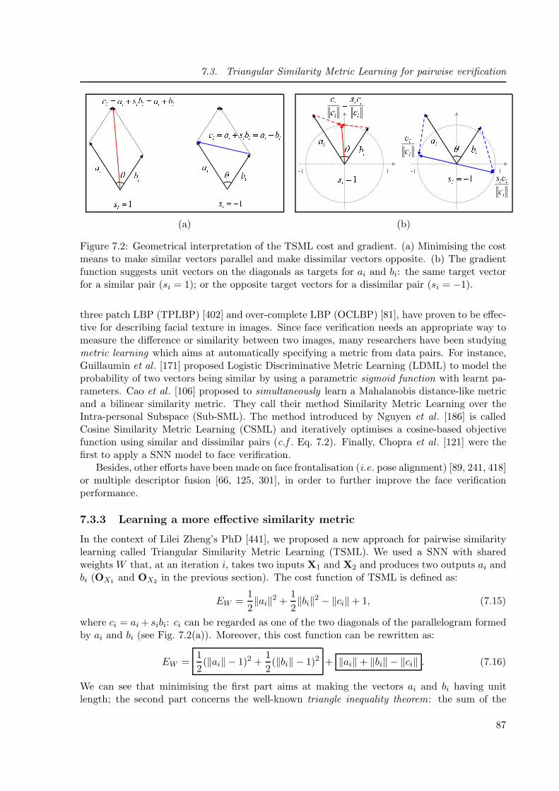
7.3. Triangular Similarity Metric Learning for pairwise verification
(a) (b)
Figure 7.2: Geometrical interpretation of the TSML cost and gradient. (a) Minimising the costmeans to make similar vectors parallel and make dissimilar vectors opposite. (b) The gradientfunction suggests unit vectors on the diagonals as targets for ai and bi: the same target vectorfor a similar pair (si = 1); or the opposite target vectors for a dissimilar pair (si = −1).
three patch LBP (TPLBP) [402] and over-complete LBP (OCLBP) [81], have proven to be effec-tive for describing facial texture in images. Since face verification needs an appropriate way tomeasure the difference or similarity between two images, many researchers have been studyingmetric learning which aims at automatically specifying a metric from data pairs. For instance,Guillaumin et al . [171] proposed Logistic Discriminative Metric Learning (LDML) to model theprobability of two vectors being similar by using a parametric sigmoid function with learnt pa-rameters. Cao et al . [106] proposed to simultaneously learn a Mahalanobis distance-like metricand a bilinear similarity metric. They call their method Similarity Metric Learning over theIntra-personal Subspace (Sub-SML). The method introduced by Nguyen et al . [186] is calledCosine Similarity Metric Learning (CSML) and iteratively optimises a cosine-based objectivefunction using similar and dissimilar pairs (c.f . Eq. 7.2). Finally, Chopra et al . [121] were thefirst to apply a SNN model to face verification.
Besides, other efforts have been made on face frontalisation (i.e. pose alignment) [89, 241, 418]or multiple descriptor fusion [66, 125, 301], in order to further improve the face verificationperformance.
7.3.3 Learning a more effective similarity metric
In the context of Lilei Zheng’s PhD [441], we proposed a new approach for pairwise similaritylearning called Triangular Similarity Metric Learning (TSML). We used a SNN with sharedweights W that, at an iteration i, takes two inputs X1 and X2 and produces two outputs ai andbi (OX1 and OX2 in the previous section). The cost function of TSML is defined as:
EW =1
2‖ai‖2 +
1
2‖bi‖2 − ‖ci‖+ 1, (7.15)
where ci = ai + sibi: ci can be regarded as one of the two diagonals of the parallelogram formedby ai and bi (see Fig. 7.2(a)). Moreover, this cost function can be rewritten as:
EW =1
2(‖ai‖ − 1)2 +
1
2(‖bi‖ − 1)2 + ‖ai‖+ ‖bi‖ − ‖ci‖ . (7.16)
We can see that minimising the first part aims at making the vectors ai and bi having unitlength; the second part concerns the well-known triangle inequality theorem: the sum of the
87

Chapter 7. Siamese Neural Networks for face and gesture recognition
Figure 7.3: Some challenging image pairs of same persons from the LFW dataset.
lengths of two sides of a triangle must always be greater than the length of the third side, i.e.‖ai‖+ ‖bi‖− ‖ci‖ > 0. More interestingly, with the length constraints induced by the first part,minimising the second part is equivalent to minimising the angle θ between the vectors of asimilar pair (si = 1) or maximising the angle θ between a dissimilar pair (si = −1), in otherwords, minimising the Cosine Similarity between ai and sibi (c.f . Eq. 7.2).
In practice, this cost function can be minimised iteratively using Stochastic Gradient Descent(SGD) and the well-known gradient Backpropagation algorithm for multi-layer neural architec-tures. The gradient of the cost function (Eq. (7.15)) with respect to the parameters W is:
∂EW
∂W= (ai −
ci‖ci‖
)T∂ai∂W
+ (bi −sici‖ci‖
)T∂bi∂W
. (7.17)
We can obtain the optimal cost at the zero gradient: ai− ci‖ci‖
= 0 and bi− sici‖ci‖
= 0. That is, the
gradient function has ci‖ci‖
and sici‖ci‖
as targets for ai and bi, respectively. Figure 7.2(b) illustrates
this: for a similar pair, ai and bi are mapped to the same target vector along the diagonal (thered solid line); for a dissimilar pair, ai and bi are mapped to opposite unit vectors along theother diagonal (the blue solid line). This perfectly reveals the objective of attracting similarpairs and separating dissimilar pairs. See [4] for more details on the optimisation procedure.
7.3.4 Experiments
7.3.4.1 Pairwise face verification results
As mentioned above, we used the LFW benchmark (‘funnelled’ version, i.e. aligned and croppedface images) to evaluate our proposed TSML approach. Both settings, the restricted and un-restricted protocol are evaluated. The restricted dataset contains fixed 300 positive and 300negative pairs, whereas in the unrestricted case we generate more pairs from the same imagesusing their identity labels. For the SNN, we considered three types of neural network architec-tures, “Linear” corresponding to a single-layer network without bias term, “Non-linear” with anadditional tanh activation function and bias and “MLP” corresponding to a two-layer network(i.e. one hidden layer) with bias and tanh activation functions. We further experimented with atraining strategy that uses only similar pairs in the optimisation, and no dissimilar pairs at all.The intuition behind this is that learning dissimilarity is challenging and not well conditioned asopposed to similarities. Thus, depending on the data, the negative term in the objective func-tion related to dissimilarity may be partly contradictory to the positive one and might inhibitthe learning of similarities during the training process. As training input, we used standard
88

7.3. Triangular Similarity Metric Learning for pairwise verification
Approaches Restricted Training Unrestricted Training
Baseline 84.83±0.38WCCN 91.10±0.45 91.17±0.36
TSML-Linear 87.95±0.40 92.03±0.38TSML-Nonlinear 86.23±0.39 91.43±0.52
TSML-MLP 84.10±0.45 89.30±0.73TSML-Linear-Sim 91.90±0.52 92.40±0.48
TSML-Nonlinear-Sim 90.58±0.52 91.47±0.37TSML-MLP-Sim 88.98±0.64 89.03±0.58
Table 7.1: Mean maxDA scores (±standard error of the mean) of pairwise face verification by theTSML-based methods on the LFW-funneled image dataset. ’-Sim’ means training with similarpairs only.
state-of-the-art Fisher Vector (FV) features [307, 342] to describe the face images and reducethem to 500 dimensions using Whitened Principal Component Analysis (WPCA).
Like the minimal Decision Cost Function (minDCF) in [170], we defined a Decision Accuracy(DA) function to measure the overall verification performance on a set of data pairs:
DA(γ) =number of right decisions (γ)
total number of pairs, (7.18)
where the threshold γ is used to make a decision on the final distance or similarity values: forthe TSML system, cos(a, b) > γ means (a, b) is a similar pair, otherwise it is dissimilar. Themaximal DA (maxDA) over all possible threshold values is the final score recorded. We reportthe mean maxDA scores (±standard error of the mean) of the 10 experiments.
Table 7.1 shows the results for a baseline method, i.e. the maxDA scores directly com-puted on the FV data, the state-of-the-art method “Within Class Covariance Normalization”(WCCN) [81], and different variants of the proposed TSML approach. It can be noted thatthe unrestricted training gives better results, in general, as more training pairs are available.Surprisingly, linear models perform better than non-linear ones. This has been confirmed byseveral other experiments and is probably due to overfitting and the lack of training data. Andfinally, the methods that train the models on only similar pairs give superior results, and alsooutperform the other baseline approaches. Note that also WCCN does not model “dissimilarity”as it minimises only the intra-class variance and not the inter-class variance.
We further compared our approach to the state of the art. For a fair comparison, all testedmethods use a single type of feature as input data. Better results could be obtained with a fusionof several types of features but, here, we wanted to focus on the different algorithms for similaritymetric learning. Table 7.2 summarises the results on the LFW face verification benchmark(restricted setting). The proposed TSML approach outperforms all existing methods. Notethat DDML (Discriminative Distance Metric Learning) is another method that we developed inthe context of Lilei Zheng’s thesis [4]. It uses a norm-based objective function and also givesexcellent results, only slightly inferior to TSML.
89

Chapter 7. Siamese Neural Networks for face and gesture recognition
Method Feature Accuracy
MRF-MLBP [65] multi-scale LBP 79.08±0.14APEM [241] SIFT 81.88±0.94APEM [241] LBP 81.97±1.90
Eigen-PEP [243] PEP 88.47±0.91Hierarchical-PEP [240] PEP 90.40±1.35
SVM [342] Fisher Vector faces 87.47±1.49DDML-Linear-Sim Fisher Vector faces 91.03±0.61
WCCN [81] Fisher Vector faces 91.10±0.45TSML-Linear-Sim Fisher Vector faces 91.90±0.52
Table 7.2: Comparison of TSML-Linear-Sim with other methods using a single type of facedescriptor under the restricted configuration with no outside data on LFW-funneled.
Approaches Restricted Training Unrestricted Training
Baseline 87.78±0.39 / 0.1335WCCN 91.69±0.29 / 0.0900 91.97±0.33 / 0.0853
TSML-Linear 89.78±0.25 / 0.1108 93.97±0.20 / 0.0648TSML-Nonlinear 87.43±0.31 / 0.1340 93.11±0.20 / 0.0733
TSML-MLP 84.88±0.24 / 0.1592 90.21±0.36 / 0.1023
TSML-Linear-Sim 92.94±0.15 / 0.0785 93.99±0.24 / 0.0662TSML-Nonlinear-Sim 91.29±0.25 / 0.0918 93.43±0.23 / 0.0690
TSML-MLP-Sim 89.59±0.45 / 0.1093 90.83±0.30 / 0.0967
Table 7.3: Mean maxDA scores (±standard error of the mean) and mean EER of pairwisespeaker verification by the TSML methods on the NIST i-vector speaker dataset. ’-Sim’ meanstraining with similar pairs only.
7.3.4.2 Results on other applications
Speaker verification
We further evaluated our TSML approach on other pairwise verification problems – forinstance, speaker verification using audio data. To this end, we used the data of the NIST2014 Speaker i-Vector Challenge [170], which consist of i-vectors [132, 158, 232] derived fromconversational telephone speech data in the NIST speaker recognition evaluations from 2004to 2012. Each i-vector, the identity vector, is a vector of 600 components, designed to becharacteristic for the voice of a given person. This dataset consists of a development set forbuilding models and a test set for evaluation. Table 7.3 shows the average maxDA scores of thedifferent variants of TSML with respect to the baseline and the state-of-the-art method WCCM.These results confirm the observations made for face verification, i.e. the linear models performbetter, and training with only similar pairs improves the performance.
Kinship verification
Another similar problem is kinship verification from images, where the objective is to de-termine whether there is a kin relation between a pair of given face images. Lu et al . [261]
90

7.3. Triangular Similarity Metric Learning for pairwise verification
Team F-S F-D M-S M-D Mean
Polito 84.00 82.20 84.80 81.20 83.10LIRIS 89.40 83.60 86.20 85.00 86.05ULPGC 85.40 75.80 75.60 81.60 80.00NUAA 84.40 81.60 82.80 81.60 82.50BIU 87.51 80.82 79.78 75.63 80.94
SILD (LBP) 78.20 70.00 71.20 67.80 71.80SILD (HOG) 79.60 71.60 73.20 69.60 73.50
Table 7.4: Kinship verification accuracy (%) on KinFaceW-II under the restricted configurationin the FG 2015 Kinship Verification Evaluation.
constructed the Kinship Face in the Wild (KinFaceW) dataset for studying the problem of kin-ship verification from unconstrained face images mostly collected from the Internet, definingfour types of relationships: Father-Son (F-S), Father-Daughter (F-D), Mother-Son (MS) andMother-Daughter (M-D). Similar to LFW, the KinFaceW dataset holds the setting of limitedtraining data for some classes and the setting of mutually exclusive training and test sets. Thereare two sub-sets: KinFaceW-I and KinFaceW-II, and besides their size, the major difference isthat any two relative faces were acquired from different photos in KinFaceW-I but most relativefaces in KinFaceW-II were captured from the same photo. In other words, environment condi-tions such as lighting differ more significantly between face pairs in KinFaceW-I than those inKinFaceW-II.
Using FV feature vectors as input, we evaluated TSML on this dataset, and, more impor-tantly, we participated in an international competition on kinship verification that was organ-ised by Lu et al . [25] in conjunction with FG 2015 and that used the KinFaceW dataset tobenchmark the submitted methods. Table 7.4 shows the verification accuracy of the differentsubmitted methods for KinFaceW-II in the restricted setting (ours is called LIRIS here). Ourapproach achieved the first place in this part of the competition. In the first part, we achievedthe third place with a mean accuracy of 82.74% behind the method from“Politecnico di Torino”(Italy) (86.30%) and the one from“Nanjing University of Aeronautics and Astronautics” (China)(82.96), both proposing a feature selection approach using different types of features and an SVMclassifier. The Side-information based linear discriminant analysis (SILD) [208] has been usedas a baseline.
7.3.5 Conclusion
The proposed TSML method represents a generic SNN-based similarity metric learning frame-work that can operate with different models – linear and non-linear and with varying complexity,making it a powerful approach for weakly supervised learning for various applications and givingstate-of-the-art results on different pairwise verification problems.
An interesting result of our studies is the fact that training with only similar pairs may im-prove the overall verification performance. Our further research work, presented in the followingsection, tries to better incorporate the negative pairs in the training process to build a morepowerful model that also exploits these dissimilarities. This will especially help in the contextof classification, which is the objective of the following work.
91

Chapter 7. Siamese Neural Networks for face and gesture recognition
Figure 7.4: Left: illustrations of some symbolic gestures that are to be recognised from inertialsensor data from mobile devices. Right: examples from the Multimodal Human Action Dataset(MHAD).
7.4 Class-balanced Siamese Neural Networks for gesture and
action recognition
7.4.1 Introduction
Our experiments showed that SNNs are able to model complex similarity metrics learnt fromdata. In the research work described in this section, that has been conducted as part of the PhDthesis of Samuel Berlemont [90] and that I have co-supervised with Christophe Garcia (LIRIS)and Gregoire Lefebvre (Orange Labs), we studied new approaches to incorporate negative, dis-similar examples in the training algorithm of SNNs, to improve the convergence and the resultingoverall embedding in the similarity space. To this end, we proposed training algorithms that gobeyond pairwise similarities and dissimilarities and operate on tuples. In addition, in this work,we were not concerned with verification but we concentrated on classification problems, i.e. wehave data samples with labelled classes, and the classes are the same at training and test time.Thus, in principle, supervised learning approaches could be used in this context. However, thereare advantages in modelling more explicitly the similarities and relationships between the dif-ferent classes using a weakly supervised metric learning approach with SNNs. That is, not onlythe overall classification performance is improved, but also new samples from unknown classescan be more effectively rejected, as we will show in this section.
The developed algorithms have been evaluated on the problems of action recognition and on3D symbolic gesture recognition using data from inertial sensors (accelerometers, gyroscopes etc.)commonly present in current mobile phones. Some of the gestures (e.g . flick east/west/north/south, pick, throw, heart, circle etc.) and activities (e.g . climbing, running, jumping etc.) aredepicted in Fig. 7.4. The solution to this problem bears a certain number of challenges. On theone hand, inertial MicroElectroMechanicals Systems (MEMS) present inherent flaws that haveto be taken into account, since they can be deceived by physical phenomena (e.g . electromagneticinterferences). On the other hand, in a real open-world application, inertial based gesture andaction recognition also has to cope with high variations between users (i.e. right/left-handedusers, dynamic/slow movements, etc.). Finally, to offer more functionality to final users, sucha recognition system should propose a large vocabulary of possible interactions and reject alluncertain decisions and parasite or irrelevant motion.
In our work, we considered a gesture or action data example as a vector of fixed size, i.e.we worked with temporally segmented samples, and we performed a pre-processing step with a
92

7.4. Class-balanced Siamese Neural Networks for gesture and action recognition
certain number of traditional filtering, resampling and normalisation techniques to reduce thenoise and to normalise the duration. More details on this can be found in [2, 33].
7.4.2 State of the art
Inertial gesture and action recognition
In the recent literature, three main strategies exist to deal with gesture and action recognitionbased on inertial data: probabilistic temporal signal modelling, temporal warping or statisticalmachine learning.
The probabilistic approach has mainly been studied with discrete [189, 207, 211] and con-tinuous HMMs [314]. For instance, Kela et al . [211] used discrete HMMs (dHMM) from gesturevelocity profiles. The first step is the input data space clustering in order to build a featurevector codebook. The second one consists in creating a discrete HMM using the sequences ofvector codebook indexes. A correct recognition rate of 96.1% is obtained with 5 HMM statesand a codebook size of 8 from 8 gestures realised by 37 users. In order to use gesture datacorrelation in time, Pylvanainen [314] proposed a system based on a continuous HMM (cHMM)achieving a recognition rate of 96.76% on a dataset with 20 samples for 10 gestures realised by7 persons.
The second approach is based on temporal warping from a set of reference gestures [64,256, 401]. Liu et al . [256] presented a method using Dynamic Time Warping (DTW) from pre-processed signal data that gives gesture recognition and user identification rates of respectively93.5% and 88%, outperforming in this study the HMM-based approach.
The third strategy is based on a specific classifier [188, 230, 404]. Hoffman et al . [188] proposea linear classifier and Adaboost, resulting in a recognition rate of 98% for 13 gestures performedby 17 participants. The study of Wu et al . [404] proposes to construct fixed-length featurevectors from the temporal input signal to be classified with Support Vector Machines (SVM).Each gesture is then segmented in time and statistical measures (mean, energy, entropy, standarddeviation and correlation) are computed for each segment to form the final feature vectors. Theresulting recognition rate is 95.21% for 12 gestures made by 10 individuals, outperforming in thisstudy the DTW results. Finally, the recent study by Lefebvre et al . [230] proposes a methodbased on Bidirectional Long-Short-Term Memory Recurrent Neural Networks (BLSTM-RNNsee [168]), which classifies sequences of raw MEM data with very good accuracy, outperformingclassical HMM and DTW methods.
We also developed a inertial gesture classification method based on supervised learning anda specific Convolutional Neural Network (CNN) model. For our dataset of 14 symbolic gestures,we obtained a classification accuracy of up to 95.8% depending on the used test protocol outper-forming other state-of-the-art methods. However, for the reasons mentioned above, i.e. betterrejection of unknown classes and improved similarity metric space, we focused our followingwork on similarity metric learning approaches with SNN models.
Rejection approaches
The notion of rejection in classification has been studied in other areas and applications.Two kinds of rejection criteria have been proposed in the literature, with the first criterionbased on the actual input to the classifier, and the second based on decision boundaries for theoutput space. Following the first strategy, Vasconcelos et al . [376], tackling handwritten digitrecognition with a neural network-based classifier, suggested to use “guard units” for each class.These units are defined by their weight vector, which is composed by the means of the features forevery training pattern belonging to the class. After activation of the network by a new sample,
93
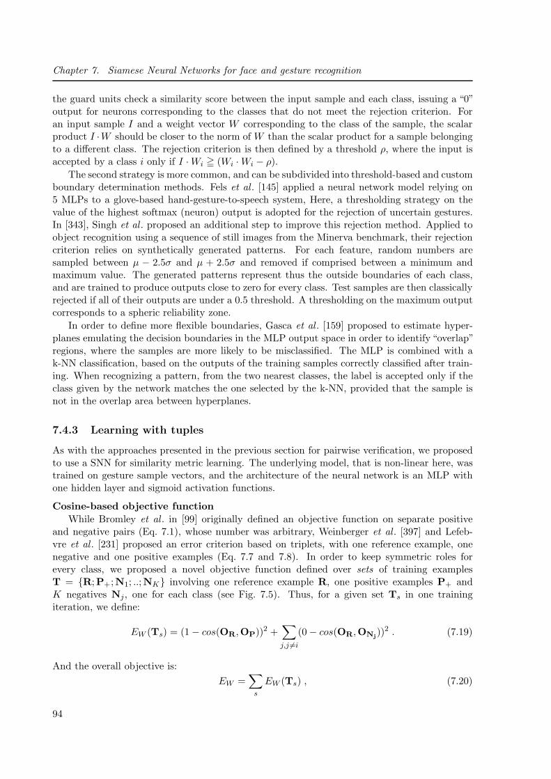
Chapter 7. Siamese Neural Networks for face and gesture recognition
the guard units check a similarity score between the input sample and each class, issuing a “0”output for neurons corresponding to the classes that do not meet the rejection criterion. Foran input sample I and a weight vector W corresponding to the class of the sample, the scalarproduct I ·W should be closer to the norm of W than the scalar product for a sample belongingto a different class. The rejection criterion is then defined by a threshold ρ, where the input isaccepted by a class i only if I ·Wi ≧ (Wi ·Wi − ρ).
The second strategy is more common, and can be subdivided into threshold-based and customboundary determination methods. Fels et al . [145] applied a neural network model relying on5 MLPs to a glove-based hand-gesture-to-speech system, Here, a thresholding strategy on thevalue of the highest softmax (neuron) output is adopted for the rejection of uncertain gestures.In [343], Singh et al . proposed an additional step to improve this rejection method. Applied toobject recognition using a sequence of still images from the Minerva benchmark, their rejectioncriterion relies on synthetically generated patterns. For each feature, random numbers aresampled between µ − 2.5σ and µ + 2.5σ and removed if comprised between a minimum andmaximum value. The generated patterns represent thus the outside boundaries of each class,and are trained to produce outputs close to zero for every class. Test samples are then classicallyrejected if all of their outputs are under a 0.5 threshold. A thresholding on the maximum outputcorresponds to a spheric reliability zone.
In order to define more flexible boundaries, Gasca et al . [159] proposed to estimate hyper-planes emulating the decision boundaries in the MLP output space in order to identify “overlap”regions, where the samples are more likely to be misclassified. The MLP is combined with ak-NN classification, based on the outputs of the training samples correctly classified after train-ing. When recognizing a pattern, from the two nearest classes, the label is accepted only if theclass given by the network matches the one selected by the k-NN, provided that the sample isnot in the overlap area between hyperplanes.
7.4.3 Learning with tuples
As with the approaches presented in the previous section for pairwise verification, we proposedto use a SNN for similarity metric learning. The underlying model, that is non-linear here, wastrained on gesture sample vectors, and the architecture of the neural network is an MLP withone hidden layer and sigmoid activation functions.
Cosine-based objective function
While Bromley et al . in [99] originally defined an objective function on separate positiveand negative pairs (Eq. 7.1), whose number was arbitrary, Weinberger et al . [397] and Lefeb-vre et al . [231] proposed an error criterion based on triplets, with one reference example, onenegative and one positive examples (Eq. 7.7 and 7.8). In order to keep symmetric roles forevery class, we proposed a novel objective function defined over sets of training examplesT = R;P+;N1; ..;NK involving one reference example R, one positive examples P+ andK negatives Nj, one for each class (see Fig. 7.5). Thus, for a given set Ts in one trainingiteration, we define:
EW (Ts) = (1− cos(OR,OP))2 +
∑
j,j 6=i
(0− cos(OR,ONj))2 . (7.19)
And the overall objective is:
EW =∑
s
EW (Ts) , (7.20)
94
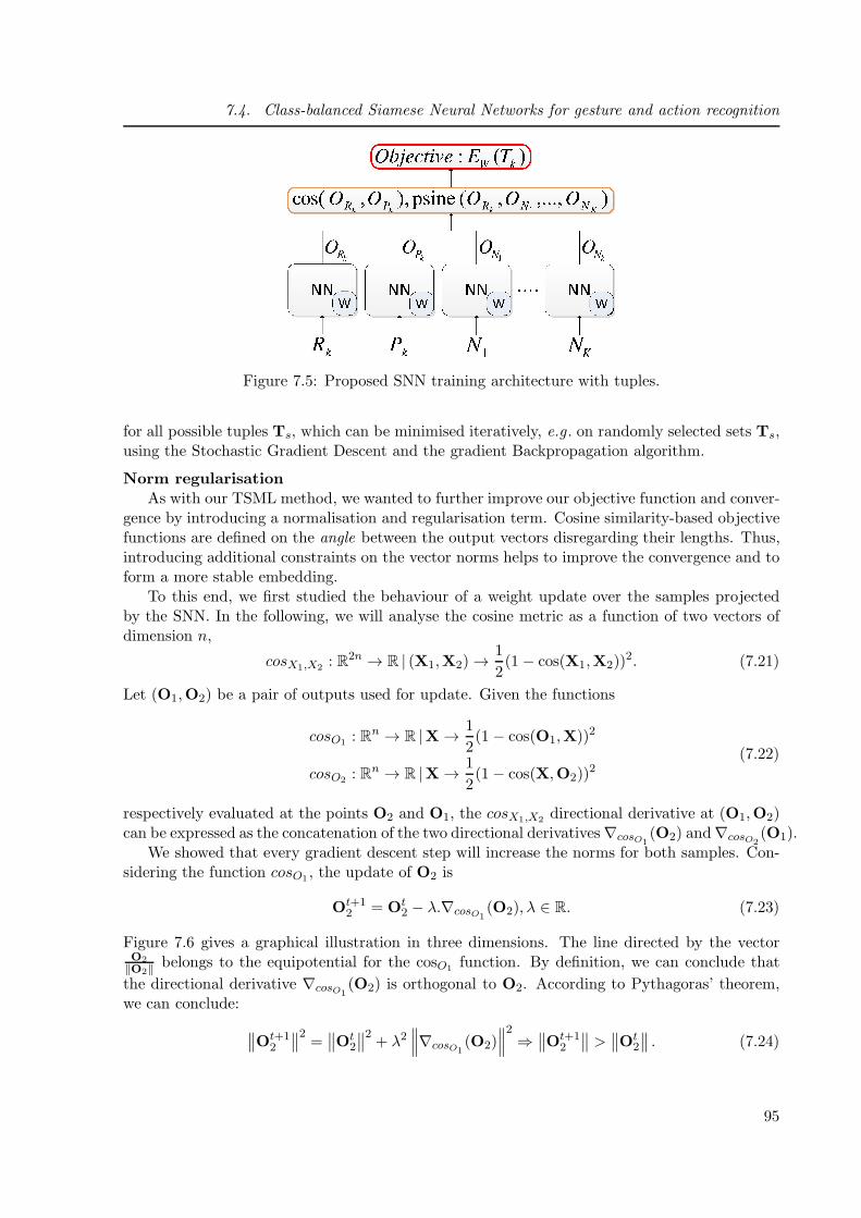
7.4. Class-balanced Siamese Neural Networks for gesture and action recognition
Figure 7.5: Proposed SNN training architecture with tuples.
for all possible tuples Ts, which can be minimised iteratively, e.g . on randomly selected sets Ts,using the Stochastic Gradient Descent and the gradient Backpropagation algorithm.
Norm regularisationAs with our TSML method, we wanted to further improve our objective function and conver-
gence by introducing a normalisation and regularisation term. Cosine similarity-based objectivefunctions are defined on the angle between the output vectors disregarding their lengths. Thus,introducing additional constraints on the vector norms helps to improve the convergence and toform a more stable embedding.
To this end, we first studied the behaviour of a weight update over the samples projectedby the SNN. In the following, we will analyse the cosine metric as a function of two vectors ofdimension n,
cosX1,X2 : R2n → R | (X1,X2)→1
2(1− cos(X1,X2))
2. (7.21)
Let (O1,O2) be a pair of outputs used for update. Given the functions
cosO1 : Rn → R |X→ 1
2(1− cos(O1,X))2
cosO2 : Rn → R |X→ 1
2(1− cos(X,O2))
2(7.22)
respectively evaluated at the points O2 and O1, the cosX1,X2 directional derivative at (O1,O2)can be expressed as the concatenation of the two directional derivatives∇cosO1
(O2) and∇cosO2(O1).
We showed that every gradient descent step will increase the norms for both samples. Con-sidering the function cosO1 , the update of O2 is
Ot+12 = Ot
2 − λ.∇cosO1(O2), λ ∈ R. (7.23)
Figure 7.6 gives a graphical illustration in three dimensions. The line directed by the vectorO2
‖O2‖belongs to the equipotential for the cosO1 function. By definition, we can conclude that
the directional derivative ∇cosO1(O2) is orthogonal to O2. According to Pythagoras’ theorem,
we can conclude:
∥∥Ot+12
∥∥2 =∥∥Ot
2
∥∥2 + λ2∥∥∥∇cosO1
(O2)∥∥∥2⇒∥∥Ot+1
2
∥∥ >∥∥Ot
2
∥∥ . (7.24)
95

Chapter 7. Siamese Neural Networks for face and gesture recognition
Figure 7.6: An update step on the projection norm for a pair (Ot1,O
t2). The sphere centre
corresponds to the origin. The grey cone represents the equipotential surface for the functioncosO1 .
Increasing the norms of the output vectors may incur progressive divergence. Moreover, withhyperbolic tangent activation functions, the output space is a hyper-cube of dimension n, whichrestricts the norms to a maximum of
√n. Therefore, we proposed to add constraints on the
norms of every output by forcing them to 1 and thus avoid any undesired saturation effects.We modify our objective function EW1 (see Eq.7.19) for a training subset Ts:
EW2(Ts) = EW1(Ts) +∑
Xp∈Ts
(1−∥∥OXp
∥∥)2. (7.25)
Given ∀(O1,O2) ∈ (Rn,Rn), cos(O1,O2) =O1·O2
‖O1‖.‖O2‖, we also propose to replace the cosine
distance for each pair by the scalar product of the pair outputs, since the norms of the twooutputs are set to one during training.
Thus, the final objective function for one training subset Ts is defined as:
EW (Ts) = (1−ORk·OPk
)2 +∑
l∈Nk
(0−ORk·ONl
)2 +∑
Xp∈Ts
(1−∥∥OXp
∥∥)2. (7.26)
This loss function can be minimised iteratively using Stochastic Gradient Descent and thegradient Backpropagation algorithm that takes into account the weight sharing and severalactivations by the different samples in each set Ts.
Since the SNN is trained to evaluate similarities between multiple samples simultaneously,our assumption was that unknown samples are projected in a feature space in a coherent mannerwith known classes. To validate this hypothesis experimentally, we proposed a new SNN rejectionstrategy explained in the following.
Proposed rejection strategiesOnce the SNN is trained, the output layer gives us a feature vector representing a similarity
measure of a set of samples. For classification of samples, any standard classifier can be appliedto these feature vectors. We choose a k-NN classification based on the cosine similarity metric inorder to prove the validity and reliability of the learned projection. Finally, our rejection criterionconsists in a single threshold, common to all classes, on the distance to the closest known sample.This same thresholding criterion is applied to another model based on DTW in order to get the
96

7.4. Class-balanced Siamese Neural Networks for gesture and action recognition
closest comparison possible and to a standard MLP, trained in a supervised way, with oneoutput neuron per class and the well-known softmax activation function. Two types of rejectionstrategies are then studied. The first kind encompasses all incorrect classifications, and tests theability of a system to identify samples whose classification is too uncertain to be accepted. Themain challenge for the model is to isolate the misclassified samples first. The second kind ofrejection concerns “unknown” classes, and aims at evaluating a model performance in isolatingelements it was not trained for from the rest of the known classes. This type rejection is onlyrarely taken into account by existing methods, or is taken care of by another model specificallytrained for this task. The main experimental results are summarised in section 7.4.5.
7.4.4 Polar sine-based objective function
While the regularised tuple-based formulation of the objective function of Eq. 7.26 is moresuited to handle angular updates, it turns out impractical when the number of classes increases.Moreover, in the derivative of the mean squared error objective, the cosine error is weighted bythe difference between the target and the cosine value which tends to zero and slows down theconvergence. Thus, we proposed a new error function that preserves the targets, while addressingboth of these problems. More specifically, we proposed a reformulation of the objective functionbased on a higher-dimensional dissimilarity measure, the polar sine metric.
Inspired by the 2D sine function, Lerman et al . [236] define the polar sine for a set Vm =v1, . . . ,vn of m-dimensional linearly independent vectors (m > n) as a normalized hyper-volume. Given A =
[v1 v2 · · · vm
]and its transpose A⊤:
PolarSine(v1, . . . ,vn) =
√det (A⊤A)∏ni=1 ‖vi‖
. (7.27)
In the special case where m = n, the matrix product in the determinant is replaced by thesquare matrix A.
Given the matrix S such that ∀(i, j) ∈ [1, .., n]2 ,Si,j = cos(vi,vj), this measure can berewritten as PolarSine(v1, . . . ,vn) =
√det (S). For numerical stability reasons during the
derivation process and to make this value independent from the number of classes, we introducedthe polar sine metric:
psine(v1, . . . ,vn) =n√
det (S). (7.28)
The polar sine metric only depends on the angles between every vector of the set. It reachesits maximum value when all the vectors are orthogonal, and thus can be used as a measure fordissimilarity.
With two comparable similarity estimators whose values are between 0 and 1, one for similarand one for dissimilar samples, it is now possible to redefine the objective function for ourtraining sets Ts:
EW3(Ts) = EsimW (Ts) + EsimW (Ts) ,
EsimW (Ts) = (1− cos(ORk,OPk
))2,
EsimW (Ts) = (1− psine(ORk,ON1 , . . . ,ONK
))2 .
(7.29)
Optimizing the polar sine corresponds to assigning a target of 0 to the cosine value of everypair of outputs from different vectors drawn in Ts\Rk, i.e. we assign a target for every pair ofdissimilar samples. This actually holds more information than our original cosine or regularisedobjective functions, which would only define a target for pairs including the reference sample.As a consequence, the psine function allows for a complete representation, in every training
97
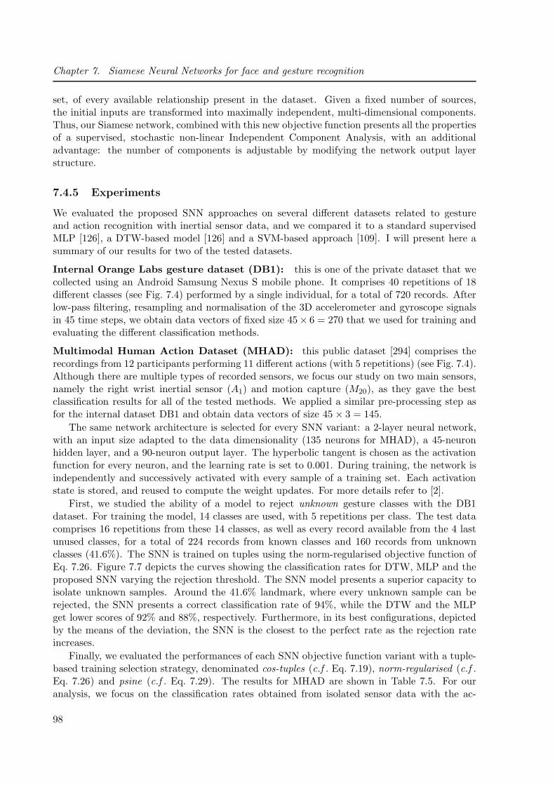
Chapter 7. Siamese Neural Networks for face and gesture recognition
set, of every available relationship present in the dataset. Given a fixed number of sources,the initial inputs are transformed into maximally independent, multi-dimensional components.Thus, our Siamese network, combined with this new objective function presents all the propertiesof a supervised, stochastic non-linear Independent Component Analysis, with an additionaladvantage: the number of components is adjustable by modifying the network output layerstructure.
7.4.5 Experiments
We evaluated the proposed SNN approaches on several different datasets related to gestureand action recognition with inertial sensor data, and we compared it to a standard supervisedMLP [126], a DTW-based model [126] and a SVM-based approach [109]. I will present here asummary of our results for two of the tested datasets.
Internal Orange Labs gesture dataset (DB1): this is one of the private dataset that wecollected using an Android Samsung Nexus S mobile phone. It comprises 40 repetitions of 18different classes (see Fig. 7.4) performed by a single individual, for a total of 720 records. Afterlow-pass filtering, resampling and normalisation of the 3D accelerometer and gyroscope signalsin 45 time steps, we obtain data vectors of fixed size 45× 6 = 270 that we used for training andevaluating the different classification methods.
Multimodal Human Action Dataset (MHAD): this public dataset [294] comprises therecordings from 12 participants performing 11 different actions (with 5 repetitions) (see Fig. 7.4).Although there are multiple types of recorded sensors, we focus our study on two main sensors,namely the right wrist inertial sensor (A1) and motion capture (M20), as they gave the bestclassification results for all of the tested methods. We applied a similar pre-processing step asfor the internal dataset DB1 and obtain data vectors of size 45 × 3 = 145.
The same network architecture is selected for every SNN variant: a 2-layer neural network,with an input size adapted to the data dimensionality (135 neurons for MHAD), a 45-neuronhidden layer, and a 90-neuron output layer. The hyperbolic tangent is chosen as the activationfunction for every neuron, and the learning rate is set to 0.001. During training, the network isindependently and successively activated with every sample of a training set. Each activationstate is stored, and reused to compute the weight updates. For more details refer to [2].
First, we studied the ability of a model to reject unknown gesture classes with the DB1dataset. For training the model, 14 classes are used, with 5 repetitions per class. The test datacomprises 16 repetitions from these 14 classes, as well as every record available from the 4 lastunused classes, for a total of 224 records from known classes and 160 records from unknownclasses (41.6%). The SNN is trained on tuples using the norm-regularised objective function ofEq. 7.26. Figure 7.7 depicts the curves showing the classification rates for DTW, MLP and theproposed SNN varying the rejection threshold. The SNN model presents a superior capacity toisolate unknown samples. Around the 41.6% landmark, where every unknown sample can berejected, the SNN presents a correct classification rate of 94%, while the DTW and the MLPget lower scores of 92% and 88%, respectively. Furthermore, in its best configurations, depictedby the means of the deviation, the SNN is the closest to the perfect rate as the rejection rateincreases.
Finally, we evaluated the performances of each SNN objective function variant with a tuple-based training selection strategy, denominated cos-tuples (c.f . Eq. 7.19), norm-regularised (c.f .Eq. 7.26) and psine (c.f . Eq. 7.29). The results for MHAD are shown in Table 7.5. For ouranalysis, we focus on the classification rates obtained from isolated sensor data with the ac-
98

7.4. Class-balanced Siamese Neural Networks for gesture and action recognition
Figure 7.7: DTW, MLP and SNN comparison with the DB1 gesture dataset.
A1 M20
DTW [126] 0.790 ± 0.107 0.888 ± 0.076MLP [126] 0.818 ± 0.099 0.913 ± 0.067SVM [109] 0.867 -
SNN cos-tuples (Eq. 7.19) 0.915 ± 0.102 0.906 ± 0.080SNN norm-regularised (Eq. 7.26) 0.886 ± 0.079 0.910 ± 0.065
SNN psine (Eq. 7.29) 0.918± 0.091 0.924 ± 0.068
Table 7.5: Classification rates of the different SNN models and the state of the art on MHAD.
celerometer A1 and the motion capture sensor M20, and we report the results for the DTW andMLP methods proposed in [126] and the SVM-based approach [109] on these same sensors. TheSNN-based approaches globally show superior results on the inertial sensor A1, with a lowestscore of 88.6% for the norm-regularised SNN, compared to a best score in the literature of 86.7%for the SVM approach. This shows that our SNN-based approach is very competitive. Thisconclusion is verified for the M20 sensor. Our SNN-psine approach, implementing the polar sinemetric and tuple-based set selection strategies contributions, gives the best result of 92.4%.
7.4.6 Conclusion
In this section, we introduced new SNN similarity metric learning methods with objective func-tions operating on tuples that are well adapted for classification problems. Our contributionson the norm regularisation term and the polar sine improved the convergence of the models, thehandling of rejection as well as the overall classification performance. We experimentally showedon gesture and action recognition applications that this approach can better cope with unknownclasses and that the polar sine-based SNN outperforms state-of-the-art methods in terms of theclassification rate.
99

Chapter 7. Siamese Neural Networks for face and gesture recognition
7.5 Conclusion
This concludes the chapter on similarity metric learning with SNN for face and gesture verifica-tion and classification. The work described here mainly focused on improving the convergenceand learning strategies for SNN based on MLP models in the context of pair-wise verificationand classification. The neural network models that we employed were rather shallow, althoughwe successfully conducted some experiments on TSML with deep CNNs for face verification [4].This is mainly due to the relatively small amount of annotated training data that is availablefor the studied applications. Deeper, more complex models would have easily overfit to thetraining data. Even with a strong regularisation, deep neural networks only show their fullpotential with large amounts of training data, and, in that case, mostly CNN-based models areused for learning deep visual feature hierarchies which is not appropriate for other types of datalike inertial signals. Finally, these relatively simple models allowed us to better understand thebehaviour of convergence and of the learnt linear and non-linear projections with respect todifferent hyper-parameters.
In the following chapter, I will present our work on person re-identification from images. Forthis application, more training data is available, and we used deeper and more complex modelsand neural network architectures in order to perform similarity metric learning and ranking ofpedestrian images.
100

8 Deep similarity metric learning
and ranking for person
re-identification
8.1 Introduction
In this chapter, I will present the work conducted in the context of the PhD thesis of YiqiangChen [116] co-supervised with Atilla Baskurt (LIRIS) and Jean-Yves Dufour (Thales Services,ThereSIS). We proposed several contributions on similarity metric learning with deep neuralnetwork models applied to the problem of person re-identification in images. The application
Figure 8.1: Illustration of person re-identification in video streams with non-overlapping views.
and problem is illustrated in Fig. 8.1. A network of cameras with non-overlapping views providescontinuous video streams where the appearing persons should be recognised within the same oracross different views and at different points in time. That is, given a query image of a personfrom one view (i.e. the probe), the goal is to re-identify this person in images from the same orfrom other views (i.e. called the gallery images).
Here, we did not work on the person detection and tracking (MOT) problem, and we con-sidered that efficient algorithms for this are available providing us with pedestrian images thatare cropped but whose identities are not matched (as illustrated in the right of Fig. 8.1).
This task bears a certain number of scientific challenges in the fields of computer visionand machine learning some of which are illustrated in Fig. 8.2. For example, the intra-classvariations can be very large due to different lighting conditions, different view points and body
101

Chapter 8. Deep similarity metric learning and ranking for person re-identification
Figure 8.2: Examples of some person re-identification challenges. Each pair of images shows thesame person except (g) and (h).
poses. Also, the images maybe of very low resolution and partial occlusions may occur frequently.Although, we assume that clothing does not change too much in a limited time frame, this maystill happen when people take off a coat or a hat or carry a bag in a different way. Also, theinter-class variation may be very small since people tend to wear similar clothes. From a machinelearning point of view, an effective model is required that is robust to the above variations andthat generalises well to persons (i.e. classes) and possibly view points that it has not beentrained for. Further, in realistic settings a query image needs to be matched to images in a verylarge gallery set. To build such models using statistical machine learning approaches, often thetraining data is very limited, and their annotation is difficult and laborious.
We employed deep neural network models for this task, because of their capacity of automat-ically and jointly learning robust visual features and classifiers. To prevent them from overfittingin this difficult setting, we used different techniques to combine supervised and weakly supervisedlearning and to include external data related to more semantic information for the given appli-cation, like semantic pedestrian attributes, body orientation or group context. I will describethese different contributions in the following.
8.2 State of the art
Approaches for person re-identification are generally composed of an appearance descriptor torepresent the person and a matching function to compare those appearance descriptors. Overthe years, numerous contributions have been made to improve both the representation as wellas the matching algorithm in order to increase robustness to the variations in pose, lighting,and background inherent to the problem. In the literature, person re-identification is mostlyperformed using the person appearance in a single colour image. However, some approaches alsouse temporal information, depth images, gait, camera topology etc.
8.2.1 Feature extraction approaches
The appearance of pedestrians from static images can be characterised according to three as-pects: colour, shape, and texture. Colour histograms are widely used to characterise colourdistributions. Also, some photometric transformation or normalisation methods are proposed:for example, Porikli et al . [311] learned a brightness transfer function, Bak et al . [77] applieda histogram equalisation technique and Liao et al . [250] applied the Retinex algorithm to pre-
102
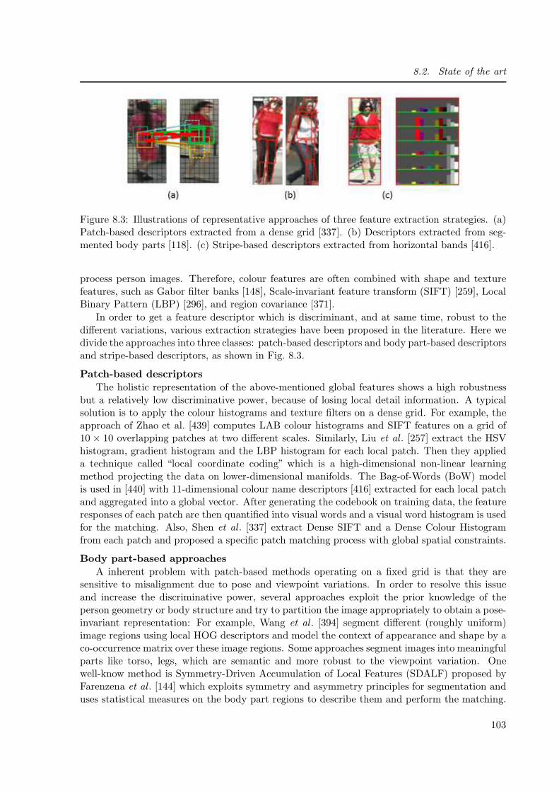
8.2. State of the art
Figure 8.3: Illustrations of representative approaches of three feature extraction strategies. (a)Patch-based descriptors extracted from a dense grid [337]. (b) Descriptors extracted from seg-mented body parts [118]. (c) Stripe-based descriptors extracted from horizontal bands [416].
process person images. Therefore, colour features are often combined with shape and texturefeatures, such as Gabor filter banks [148], Scale-invariant feature transform (SIFT) [259], LocalBinary Pattern (LBP) [296], and region covariance [371].
In order to get a feature descriptor which is discriminant, and at same time, robust to thedifferent variations, various extraction strategies have been proposed in the literature. Here wedivide the approaches into three classes: patch-based descriptors and body part-based descriptorsand stripe-based descriptors, as shown in Fig. 8.3.
Patch-based descriptors
The holistic representation of the above-mentioned global features shows a high robustnessbut a relatively low discriminative power, because of losing local detail information. A typicalsolution is to apply the colour histograms and texture filters on a dense grid. For example, theapproach of Zhao et al. [439] computes LAB colour histograms and SIFT features on a grid of10 × 10 overlapping patches at two different scales. Similarly, Liu et al . [257] extract the HSVhistogram, gradient histogram and the LBP histogram for each local patch. Then they applieda technique called “local coordinate coding” which is a high-dimensional non-linear learningmethod projecting the data on lower-dimensional manifolds. The Bag-of-Words (BoW) modelis used in [440] with 11-dimensional colour name descriptors [416] extracted for each local patchand aggregated into a global vector. After generating the codebook on training data, the featureresponses of each patch are then quantified into visual words and a visual word histogram is usedfor the matching. Also, Shen et al . [337] extract Dense SIFT and a Dense Colour Histogramfrom each patch and proposed a specific patch matching process with global spatial constraints.
Body part-based approaches
A inherent problem with patch-based methods operating on a fixed grid is that they aresensitive to misalignment due to pose and viewpoint variations. In order to resolve this issueand increase the discriminative power, several approaches exploit the prior knowledge of theperson geometry or body structure and try to partition the image appropriately to obtain a pose-invariant representation: For example, Wang et al . [394] segment different (roughly uniform)image regions using local HOG descriptors and model the context of appearance and shape by aco-occurrence matrix over these image regions. Some approaches segment images into meaningfulparts like torso, legs, which are semantic and more robust to the viewpoint variation. Onewell-know method is Symmetry-Driven Accumulation of Local Features (SDALF) proposed byFarenzena et al . [144] which exploits symmetry and asymmetry principles for segmentation anduses statistical measures on the body part regions to describe them and perform the matching.
103

Chapter 8. Deep similarity metric learning and ranking for person re-identification
Bak et al . [77] proposed an approach based on spatial covariance regions which are segmentedusing 5 HOG-based body part detectors. To better exploit the prior knowledge of plausiblebody part configurations, Cheng et al . [118] used Pictorial Structures to localise the body partsand match their descriptors based on HSV histograms and Maximally Stable Colour Regions(MSCR).
Stripe-based approachesIn most settings, pedestrians are seen from an arbitrary horizontal viewpoint. Thus, some
methods extract features on horizontal stripes and are thus invariant to large horizontal shiftsin the image. Gray et al . [169] first proposed to divide the pedestrian image into 6 equally-sizedhorizontal stripes. The approximately correspond to the image regions of the head, upper andlower torso, upper and lower legs and fee. In each stripe, 8 colour channels (RGB, HS, YCbCr)and 19 texture channels (Gabor and Schmid filter banks) are represented. Similarly, Mignon etal . [278] build the feature vector from RGB, YUV and HSV channels and the LBP texturehistograms in horizontal stripes. Yang et al . [416] also proposed to use 6 stripes and introducedthe salient colour name-based colour descriptor (SCNCD) for pedestrian colour descriptions. Theapproach proposed by Ma et al. [264] computes covariance matrices on Gabor filter responses atdifferent scales and on different image bands, and the difference of these matrices on consecutivebands is used to build the model. Finally, Liao et al . [250] proposed LOcal Maximal Occurrence(LOMO) features that we also used in our work. Scale-Invariant Local Ternary Patterns (SILTP)and HSV histograms are extracted on each line of the image at different scales, and then onlythe maximum value is retained for each line.
8.2.2 Matching approaches
Based on the extracted features, we can distinguish two types of matching methods. The firstconsists of learning a matching function in a supervised manner, and the other learns a distancemetric in feature space.
Matching function learning
Given feature based representations of a pair of images, an intuitive approach is to computethe geodesic distance between the descriptors, for instance, using the Bhattacharyya distancebetween the histogram-based descriptors or the L2-norm between descriptors in a Euclideanspace. However, some features may be more relevant for appearance matching than others.Therefore, several approaches have been proposed to learn a matching function in a supervisedmanner from a dataset of image pairs.
For instance, the method of Schwartz and Davis [334] transforms the high-dimensional fea-tures into low-dimensional discriminant vectors using Partial Least Squares (PLS) in a one-against-all scheme. Lin et al . [251] proposed an approach based on the Kullback-Leibler di-vergence of feature distributions of two images and pairwise dissimilarity profiles learnt fromtraining data. Gray et al . [169] use boosting to find the best ensemble of localised featuresfor matching. And Prosser et al . [313] proposed an ensemble of RankSVMs to solve personre-identification as a ranking problem.
Metric learningCompared to standard generic distance measures, e.g . the Euclidean or Bhattacharyya dis-
tance, a metric that is learnt specifically for person images is more discriminative for the giventask of re-identification and more robust to large variations of person images across views.
Most distance metrics learning approaches learn a Mahalanobis-like distance: D2(x, y) =(x−y)TM(x−y) where M is a positive semi-definite (PSD) matrix of which the elements are to
104

8.2. State of the art
be learnt. Several works factorise M as M = wTw, ensuring the PSD constraint and implicitlydefining a (potentially low-dimensional) projection into an Euclidean space which reflects thedistance constraints. We distinguish two types of methods explained in the following.
The first class of methods generally defines an objective function based on distance con-straints. The global idea of constraints is to keep all the vectors of the same class closerwhile pushing vectors of different classes further apart. M is solved by a constrained convexoptimisation method. For example, Mignon et al . [278] presented a method called PairwiseConstrained Component Analysis (PCCA), and Zheng et al. [443] proposed the ProbabilisticRelative Distance Comparison (PRDC) model, both defining pair-wise constraints. In contrast,the approach of Dikmen et al. [134] called Large Margin Nearest Neighbour classification withRejection (LMNN-R) operates on constraints that are defined on the neighbourhood of exam-ples. To avoid the tedious iterative optimisation procedure, Koestinger et al . [216], in their“Keep It Simple and Straightforward Method” (KISSME), propose a formulation that allows fora closed-form solution of the matrix M .
The methods of the second class are generally variants of the Linear Discriminative Analysis(LDA). The approaches are based on the difference of the feature vectors of two classes. Thepositive class consists in pairs of images of the same person acquired by different cameras, andthe negative class consists in pairs of images of different person acquired by different cameras.They learn directly the projection w to a discriminative low-dimensional subspace where thebetween-class variance is maximised and the within-class variance is minimised. In LDA, the
objective function is formulated as: J(w) = wTSbwwTSww
, where Sb and Sw are the between-class andwithin-class scatter matrices, respectively. Methods belonging to this class are LFDA proposedby Pedagadi et al . [303] combining LDA and Locality-Preserving Projection for dimensionalityreduction, the Cross Quadratic Discriminitive Analysis (XQDA) metric by Liao et al. [250]combining Quadratic Discriminative Analysis (QDA) and KISSME and the Null Foley-SammonTransform (NFST) by Zhang et al. [434].
8.2.3 Deep learning approaches
Methods based on deep neural networks jointly learn discriminative features and a matchingfunction or a similarity metric. Several approaches have been presented in the literature.
8.2.3.1 Architectures
Some deep learning architectures are conceived to operate on stripes over the input image. Forexample, Yi et al . [420] first applied a CNN on re-identification. Given two person images,they are first separated into three over-lapped horizontal stripes respectively, and the imagepairs are matched by three Siamese Convolutional Neural Networks (SCNN). Varior et al . [374]proposed to integrate a gating layer in a SCNN to compare the extracted local patterns foran image pair at the medium-level and propagate more relevant features to the higher layersof the network. Spatial dependency between stripes are exploited in [375] by a Long ShortTerm Memory (LSTM) network operating on LOMO [250] and SCNCD [416] features extractedon horizontal stripes. Cheng et al . [117] proposed to combine the global and stripe featureextraction using a multi-channel CNN model operating on different parts of the image.
Some methods directly integrate some kind of patch matching into a CNN architecture tohandle misalignment and geometric transformations. For instance, Li et al . [247] proposed anarchitecture called Filter pairing neural network directly performing the patch matching usingintegrated displacement matrices. However, this architecture is computationally complex and
105

Chapter 8. Deep similarity metric learning and ranking for person re-identification
has thus been simplified by Ahmed et al. [61] introducing a cross-input neighbourhood differencelayer.
Other methods integrate a body part-based feature extraction within a deep neural net-work architecture. Zhao et al . [437], for example, proposed an architecture composed of threecomponents: a body region proposal network (locating human body joints), a feature extractionnetwork and a feature fusion network. However, this requires training data with annotated bodyparts. In contrast, Li et al . [239] proposed to localise latent pedestrian parts through SpatialTransform Networks (STN) [199]. Zhao et al . [438] proposed to jointly model the human bodyregions that are discriminative for person matching with neither prior knowledge nor labelleddata and compute a compact representation. An image feature map is first extracted by adeep Fully Convolutional Neural network (FCN), and discriminative features are automaticallydetected and extracted in several network branches to perform the matching, which has beentrained using a siamese structure and triplets of examples.
8.2.3.2 Objective functions
As we have seen in the previous chapter, by appropriately defining objective functions, one canlearn a non-linear projection into a feature space in which the similarity of pedestrian is wellrepresented. In the following, we will rather use the term “loss function” as it is common in therecent literature for deep neural networks since there is often no regularisation term. Severalloss functions for person re-identification exist in the literature. Yi et al . [420] used the devianceloss in a Siamese network, as follows:
Edeviance = ln(e−2sl + 1), (8.1)
where −1 6 s 6 1 is the similarity score and l = 1 or −1 is the label (c.f . Eq. 7.9). And in [61,247], the re-identification task is considered as an image pair classification problem decidingwhether an image pair is from the same person or not. Ding et al . [135] first applied the tripletloss (c.f . Eq. 7.7) to train a CNN for person re-identification. Some methods combine differentobjective functions to improve the performance. For example, Cheng et al . [117] proposed animproved variant of the triplet loss function combining it with the contrastive loss. Zheng etal . [444] combined an image pair classification loss and the contrastive loss (c.f . Eq. 7.4,7.6).And Chen et al . [113] applied a quadruplet loss which samples four images from three identitiesand minimises the difference between a positive pair from one identity and a negative pair fromtwo different identities and they combine this quadruplet loss with the triplet loss.
8.2.4 Evaluation measures
The Cumulated Matching Characteristics (CMC) curve and the mean Average Precision (mAP)are the two most widely used evaluation measures for person re-identification.
CMC evaluates the top n nearest images in the gallery set with respect to one probe image.If a correct match of a query image is at the kth position (k <= n), then this query is consideredas success of rank n. A curve can thus be drawn for varying n, with n in the x-axis and theproportion of correct matches in the y-axis. Also, we denote the CMC curve value at a givenrank n the “Rank n score”.
mAP is the mean value of the average precision of all queries. The average precision isdefined as the area under the Precision-Recall curve.
106

8.3. Leveraging additional semantic information – attributes
8.3 Leveraging additional semantic information – attributes
8.3.1 Introduction
As in previous work in the literature [117, 135, 419], we proposed to tackle the person re-identification problem with a similarity metric learning approach based on SNNs since the classesare not known a priori and since we would like to directly learn from data a generic (non-linear) metric between image pairs that robustly expresses the similarities (and dissimilarities)of persons. Re-identification of a given query image is then performed by computing this metricon all images in the gallery set and returning the one(s) with the smallest distance.
Our first contribution consisted in building a SNN-based model that is trained on tripletsand that incorporates semantic attributes in order to assist the re-identification improving itsperformance [3, 15]. The idea is that such mid-level attributes, like gender, accessories andclothing, represent characteristic features that are highly invariant to view point, body pose andother image variations. Moreover, they could be used for so-called “zero-shot” identification, i.e.querying by an attribute-based description instead of an image. Since biometric features likefaces are often not visible or of too low resolution to be helpful in surveillance, pedestrian at-tributes could be considered as soft-biometrics and provide additional discriminant information.
Our proposed approach first trains a multi-class CNN in a supervised way to recognise aset of pre-defined person attributes from images and then combines this neural network with aSNN trained in a weakly supervised way on triplets to model a similarity metric between personimages.
8.3.2 State of the art
8.3.2.1 Attribute recognition
In the pioneering work of Vaquero et al . [373], the person image is segmented into regions, andeach region is associated with a classifier based on Haar-like features and dominant colours.Layne et al . [227] annotated 15 attributes on the VIPeR dataset and proposed an approach toextract a 2784-dimensional low-level colour and texture feature vector for each image and to trainan SVM for each attribute. The method of Zhu et al . [448] determines the upper and lower bodyregions according to the average image and extracts colour and texture features (HSV, MB-LBP,HOG) in these two regions. Then, an Adaboost classifier is trained on these features to recogniseattributes. The drawback of these approaches is that all attributes are treated independently.That is, the relation between different attributes is not taken into account. Zhu et al . [449]tried to overcome this limitation by introducing an interaction model based on their Adaboostapproach [448] learning an attribute interaction regressor. The approach from Deng et al . [133]used a Markov Random Field (MRF) for this purpose.
Some CNN models have also been proposed for pedestrian attribute recognition, e.g . the oneby Li et al . [238] based on CaffeNet and Sudowe et al . [358] called Attribute Convolutional Net(ACN). Zhu et al . [450, 451] proposed to divide the pedestrian images into 15 overlapping partswhere each part connects to several CNN pipelines with several convolution and pooling layers.
8.3.2.2 Re-identification with attributes
Some works have used pedestrian attributes to assist with the re-identification task, e.g . theSVM-based approach of Layne et al . [227]. In their approach, the final distance between twopedestrian images is computed as a weighted sum of low-level feature distance and attribute
107

Chapter 8. Deep similarity metric learning and ranking for person re-identification
Figure 8.4: Overview of our pedestrian attribute recognition approach.
distance. Li et al . [237] embedded middle-level clothing attributes via a latent SVM frameworkfor more robust person re-identification. The approach introduced by Khamis et al . [213] learnsa discriminative projection into a joint appearance-attribute subspace in order to leverage theinteraction between attributes and appearance for matching.
The approach of Zhu et al . [450] recognises attributes with deep neural networks then cal-culates a pedestrian distance by weighting the attribute distance and a low-level feature-basedperson appearance distance. McLaughlin et al . [276] proposed to perform person re-identificationand attribute recognition in a multi-task learning. Their loss function is a weighted sum of theattribute and identification classification loss as well as a Siamese loss. They show that thismulti-task joint learning improves the re-identification performance. Matsukawa et al . [275]proposed to fine-tune the well-known Alexnet with attribute combination labels to increase thediscriminative power. Further they concatenated the CNN embedding directly with LOMO fea-tures and used the metric learning method XQDA [250] to learn a feature space. Su et al . [356]presented a three-stage procedure that pre-trains a CNN with attribute labels of an independentdataset, then fine-tunes the network with identity labels and finally fine-tunes the network withthe learned attribute feature embedding on the combined dataset. The main difference of theseapproaches to ours is the way of making use of attributes to assist in the re-identification task.
8.3.3 Attribute recognition approach
8.3.3.1 Overall procedure and architecture
The architecture of the proposed attribute recognition approach is shown in Fig. 8.4. Theframework consists of two branches. One branch is a CNN extracting higher-level discrimi-native features by several succeeding convolution and pooling operations that become specificto different body parts at a given stage (P3) in order to account for the possible displace-ments of pedestrians due to pose variations. Another branch extracts the viewpoint-invariantLocal Maximal Occurrence (LOMO) features, a robust visual feature representation that hasbeen specifically designed for viewpoint-invariant pedestrian attribute recognition and achievingstate-of-the-art results [250]. The extracted LOMO features are then projected into a linear sub-space using Principal Component Analysis (PCA) and then fused with the CNN output using
108

8.3. Leveraging additional semantic information – attributes
a fully-connected layer and a final (fully-connected) output layer with one neuron per attributeto recognise.
The architecture of the CNN is a succession of convolution and max pooling layers that isrelatively standard in the literature, up to the pooling layer P3. At this stage (P3), we proposeto divide the resulting feature maps vertically into 4 equal parts roughly corresponding to theregions of head, upper body, upper legs and lower legs. For each part, similar to [375], we usetwo layers (C4, C5) with 1D horizontal convolutions of size 3×1 without zero-padding reducingthe feature maps to single column vectors. These 1D convolutions allow to extract high-leveldiscriminative patterns for different horizontal stripes of the input image. In the last convolutionlayer, the number of channels is increased to 150, and these feature maps are given to a fully-connected layer (fc1) to generate an output vector of dimension 500. All the convolution layersin our model are followed by batch normalisation and ReLU activation functions.
We experimentally showed that this specific CNN architecture as well as the fusion of thesediscriminant deep features with the more “invariant” LOMO features provides a powerful modelfor pedestrian attribute recognition giving state-of-the-art results on public benchmarks.
8.3.3.2 Training
The proposed CNN is trained in a supervised way using a dataset of pedestrian images withannotated attributes. The weights are initialised at random and updated using Stochastic Gra-dient Descent minimising the global loss function (Eq. 8.2) on the given training set. Since mostattributes are not mutually exclusive, i.e. pedestrians can have several properties at the sametime, the attribute recognition is a multi-label classification problem. Thus, the multi-labelversion of the sigmoid cross entropy is used as the overall loss function:
E = − 1
N
N∑
i=1
L∑
l=1
[wlyil log(σ(xil)) + (1− yil) log(1− σ(xil)] , (8.2)
with σ(x) =1
1 + exp(−x) ,
where L is the number of labels (attributes), N is the number of training examples, and yil, xilare respectively the lth label and classifier output for the ith image. Usually, in the training set,the two classes for an attribute are highly unbalanced. That is, for most attributes, the positivelabel appears generally less frequently than the negative one. To handle this issue, we added aweight w to the loss function: w = −log2(pl) , where pl is the positive proportion of attribute lin the dataset.
8.3.4 Attribute-assisted person re-identification
8.3.4.1 Overall approach
We proposed a new CNN-based similarity metric learning approach for pedestrian re-identi-fication [3, 15] that effectively combines automatically learned visual features with semanticattributes, extracted by our method described in the previous section. The overall frameworkis shown in Fig. 8.5. The framework is composed of two neural networks that are pre-trained.The first is a deep CNN that is trained in a supervised way to classify identities on a separatetraining set using the softmax cross-entropy loss:
Eidentification = −N∑
k=1
yklog(P (yk = 1|x)) with (8.3)
109

Chapter 8. Deep similarity metric learning and ranking for person re-identification
Figure 8.5: Overall architecture of our attribute-assisted re-identification approach.
P (yj = 1|x) = eWTj x+bj
∑Nk=1 e
WTkx+bk
(8.4)
(For more details refer to [20]). Then we remove the output classification layers of the networkand keep the other parts of the network which are related to feature selection. The second partis our attribute recognition network that is trained as described in the previous section (andwithout the LOMO features). After training, we also remove the output layers and keep allthe other layers up to the first fully-connected layer (fc1). The output vectors from the hiddenlayers of the two CNNs represent high-level features related to attributes and pedestrian identitiesrespectively. In order to combine the extracted features effectively, we propose to integrate bothoutput vectors in a new neural network that automatically learns these fusion parameters onthe re-identification task in a triplet architecture (described in the next section). This leadsto a fully neural architecture that can be trained and fine-tuned as a whole to maximise there-identification performance.
8.3.4.2 Fusion by triplet architecture
The pre-trained attribute CNN and identification CNN are combined (using their intermediatefully-connected layers fc1 and adding a new fully-connected layer) and trained in a triplet ar-chitecture (see Fig. 8.5). Here, we proposed to use an improved triplet loss with hard exampleselection to learn the optimal fusion of the two types of features. Unlike the classical tripletloss, a (K +2)-tuple of images instead of a triplet is projected into the feature space. The tupleincludes one reference image R, one positive image P+ and K negative images Nj. With their
110

8.3. Leveraging additional semantic information – attributes
Accuracy Rate (%) Recall@FPR=0.1 AUCMRFr2[133] DeepMar[238] mlcnn[451] ours mlcnn[451] ours mlcnn[451] ours
80.8 85.4 86.6 90.0 65.6 79.9 87.0 93.0
Table 8.1: Attribute recognition results on PETA (in %).
respective CNN output vectors OR, OP and ONj, this constraint is defined as:
min(‖OR −ONj‖22)− ‖OR −OP‖22> m , (8.5)
with m being a margin (set to 1 in our experiments). Similarly to the distance learning approach“Top-push” proposed by [425] , hard example mining in [61, 332] or moderate positive examplemining in [338], the idea is to find the most appropriate example(s) to update the model. Thenegative example that is closest to the reference is considered the hardest example and havingthe highest potential for improvement. The network is thus updated efficiently by pushing thehardest example further away from the reference. The intuition is that if the positive example isranked in front of the hardest negative example then the positive example is ranked first, whichis our goal. In classic triplet loss, a large part of triplets does not violate the triplet constraint(c.f . Eq. 8.5). Thus, these triplets are useless for learning. The selection among K negativeexamples reduces the number of unused training data and can make the training more efficient.
To further enhance the loss function, as an extension of [117], we added a term includingthe distance between the reference example and the positive example. The loss function (called”min-triplet“ loss) of one iteration is defined as:
Emin−triplet = −max(‖OR −OP ‖22−minj
(‖OR −ONj‖22) +m, 0) + α‖OR −OP‖2 . (8.6)
The first part of the loss is a comparison of two distances which defines a relative relationship inthe feature space. The second part corresponds to an absolute distance in feature space weightedby a factor α (set to 0.02 in our experiments). Combining these two constraints leads to a moreefficient learning of the resulting manifold that better represents the semantic similarities.
Using this loss function, we trained the additional fully-connected layer for the fusion, and,at the same time, we fine-tune the other parts of the network, i.e. the weights are updated ata lower rate. Unlike other approaches[213, 227, 237, 276], the advantage of our method is thatthe attributes do not need to be annotated on the re-identification dataset. We can make use ofa separate dataset with annotated attributes and transfer this information to a re-identificationdataset by fine-tuning.
8.3.5 Experiments
We first evaluated the accuracy of our attribute recognition approach on three different datasets:PETA (19 000 images, 65 attributes), APiS (3661 images, 11 attributes) and VIPeR (632 images,21 attributes) (see Fig. 8.6) using the evaluation protocols proposed in the literature. Theevaluation measures are the accuracy, the average recall at a False Positive Rate (FPR) of 0.1and the Area Under Curve (AUC) of the average Receiver Operating Characteristic (ROC)curve. The results in Tables 8.1-8.3 show that our approach outperforms all state-of-the-artmethods: MRFr2 [133], DeepMar [238], mlcnn [451], fusion [448], interact [449] and svm[227].
111

Chapter 8. Deep similarity metric learning and ranking for person re-identification
Figure 8.6: Some example images from pedestrian attribute datasets.
Accuracy Recall@FPR=0.1 AUCours fusion[448] interact[449] ours fusion[448] interact[449] DeepMar[238] ours
89.3 62.1 64.7 72.7 86.7 87.2 90.0 89.5
Table 8.2: Attribute recognition results on APiS (in %).
Then we evaluated our attribute-assisted person re-identification framework on the publicCUHK03 dataset [247] containing 13 164 images of 1 360 pedestrians (automatically cropped bya person detection algorithm). We pre-trained the attribute CNN branch on the Peta dataset,and the identity CNN branch on CUHK03 (the identities of the test set are different from thetraining set). Our evaluation criterion for re-identification is the proportion of test (query)images for which rank=n, i.e. in the ranking according to the Euclidean distance in the learntprojection space, a correct match is within the first n images. Table 8.4 shows the resultsfor rank=1,5,10 compared to the state of the art on the CUHK03 (“detected”) dataset. Ourapproach outperformed all other methods showing the effectiveness of our SNN similarity metriclearning framework with improved triplet loss. One can also see the significant contribution ofthe attributes to the overall performance.
8.3.6 Conclusion
In this section, I presented our recent work on person re-identification showing that the useof additional semantic information (the attributes) can considerably improve the performanceof similarity metric learning. Our first contribution was a powerful framework for attributerecognition fusing discriminant deep CNN features trained on pedestrian images with highlyinvariant LOMO features and achieving state-of-the-art classification accuracy on three publicdatasets. Then, by using both identity and attribute information and also an improved tripletobjective function with hard negative examples and finally by employing effective pre-trainingand fusion strategies on appropriate CNN architectures, we were able to obtain state-of-the-art
112

8.4. A gated SNN approach
Accuracy Recall@FPR=0.2 AUCsvm[227] mlcnn[450] ours svm[227] mlcnn[450] ours ours
68.9 74.1 83.9 56.1 65.5 69.6 80.9
Table 8.3: Attribute recognition results on VIPeR (in %).
Method rank=1 rank =5 rank =10
FPNN [247] 19.9 49.3 64.7Convnet [61] 45.0 75.3 83.4
LOMO+XQDA [250] 46.3 78.9 88.6SS-SVM [436] 51.2 80.8 89.6SI-CI [386] 52.2 84.3 92.3DNS[434] 57.3 80.1 88.3
S-lSTM [375] 57.3 80.1 88.3S-CNN SQ [374] 61.8 80.9 88.3
CAN[255] 63.1 82.9 88.2
ours Identity only 59.7 86.1 93.3ours fusion Id&Attr 65.0 90.3 95.1
Table 8.4: Re-identification result on CUHK03 (“detected”).
results on challenging public benchmarks.
8.4 A gated SNN approach
8.4.1 Introduction
In the previous section, we saw one way of introducing prior knowledge into the SNN model,i.e. by pre-training a neural network on labelled data and fusing and fine-tuning the model intoa larger neural network that learns the final similarity metric. In this section, I will describeanother original approach that we proposed [17], which also uses a supervised pre-trained modelon external semantic information but is based on a different neural architecture. In the precedingarchitecture, two neural networks are pre-trained in a supervised manner on two different labelleddatasets (one for identification, one for attributes). In the model that I will present here, thereare two neural networks (i.e. two branches) with some common layers in the beginning, and thetraining is done simultaneously with a loss function integrating the two different objectives; aso-called multi-task learning. Moreover, one branch acts as a gate to “steer” which part of theother branch should be activated.
In our re-identification application, one branch is a CNN pre-trained for person identification,and the other branch, the gating branch, is pre-trained for person body orientation estimation.The whole combined neural network model is then fine-tuned for person re-identification. Inthe following, we will first described the related work and then explain our approach, calledOrientation-Specific CNN (OSCNN), in more detail.
113

Chapter 8. Deep similarity metric learning and ranking for person re-identification
8.4.2 State of the art
Most existing methods for person re-identification focus on developing a robust representation tohandle the variations of view. Some methods take into account the view as extra information. Forexample, Ma et al . [266] divide the data according to the additional camera position informationand learn a specific distance metric for each camera pair. Lisanti et al . [252] proposed to applyKernel Canonical Correlation Analysis which finds a common subspace between the featurespace from disjoint cameras. Yi et al . [420] proposed to apply a Siamese CNN to person re-identification. Similar to [252], the weights of two subnetworks are not shared to learn a cameraview projection to a common feature space. In these approaches, camera information is usedbut the body orientation which is only partly due to different camera views is not modelled.That is, in the same camera view, pedestrians can exhibit different orientations and thus largelydifferent appearances in the resulting images.
In order to solve this issue, Bak et al . [78] perform an orientation-driven feature weightingand the body orientation is calculated according to the walking trajectory. some other ap-proaches [330, 378] deal with the orientation variations of pedestrian images by using Mixtureof Experts. The expert neural networks map the input to the output, while a gating networkproduces a probability distribution over all experts’ final predictions. Verma et al . [378] appliedan orientation-based mixture of experts to the pedestrian detection problem. Sarfraz et al . [330]proposed to learn the orientation sensitive units in a deep neural network to perform attributerecognition. Garcia et al . [157] used orientations estimated by a Kalman filter and then trainedtwo SVM classifiers for pedestrian images matching with respectively similar orientations anddissimilar orientations. And the approach of Li et al . [245] learns a mixture of experts, wheresamples were softly distributed into different experts via a gating function according to theviewpoint similarity.
Sharing the idea of mixture of experts, we proposed to build a multi-domain representationin different orientations with deep CNNs. Intuitively, an orientation-specific model should havea better generalisation ability than a camera view-specific model, since we cannot incorporateall possible surveillance camera views. Further, instead of using discrete orientations for thegating activation function, in our method, we use a regression model to estimate an accurateand continuous body orientation. This allows to continuously weight different expert models forre-identification and also avoids combining contradictory orientations at the same time.
8.4.3 Body orientation-assisted person re-identification
8.4.3.1 Model architecture
The overall procedure of our re-identification approach OSCNN is shown in Fig. 8.7. Thenetwork contains an orientation gating branch and a re-identification branch consisting of 4feature embeddings regarding the 4 main orientations: left, right, frontal and back. The finaloutput feature representation is a linear combination of the four expert outputs and is steeredby an orientation gate unit which is a function of the estimated orientation.
The proposed neural network architecture consists of two convolution layers shared betweenthe two branches. In the re-identification branch, there are 3 further convolution layers followedby 4 separate, parallel fully-connected layers (left,right,front,back) of 512 dimensions, each onecorresponding to a local expert. Thus, our network learns different projections from differentorientation domains to a common feature space.
In the orientation regression branch, 2 convolution layers and 2 fully connected layers areconnected to the common convolutional layers. The estimated orientation output by the ori-
114

8.4. A gated SNN approach
Figure 8.7: Overview of the OSCNN architecture.
entation gating branch is represented by a two-dimensional Cartesian vector [α, β] constructedby projecting the orientation angle on the left-right axis (x) and on the front-back (y) axis andthen normalising it to a unit vector. Based on this vector, the orientation gate selects andweights either the left or the right component and either the front or the back component ofthe re-identification branch. Let fleft,right,front,back be the output feature vectors of the 4 dif-ferent orientation branches. The final re-identification output vector is the sum of the left-rightcomponent and the front-back component:
fouput = max(α, 0)fleft +max(−α, 0)fright +max(β, 0)ffront +max(−β, 0)fback (8.7)
Different from the classic mixture of experts approach, our orientation gate is set before the localexperts, and we perform a regression instead of a classification. The advantage of our orientationgate is that it avoids combining contradictory orientations like front and back. Computationally,only two among four orientations are used and combined according to the sign of α and β. Thisfurther allows saving computation.
8.4.3.2 Training
There are two stages to train the model, explained in the following.
Multi-task network pre-training
In the first stage, the orientation regressor and a general re-identification feature embeddingare both trained in parallel with two separate objective functions.
We start training the network with pedestrian identity labels and orientation labels respec-tively. The identification branch is trained as in our attribute-assisted model in section 8.3.4, i.e.using the cross-entropy loss Eidentification (Eq. 8.3) on the softmax output and identity-labelledperson images.
For the body orientation, we use the Euclidean loss to train the orientation regression of αand β. For a given training example, we have:
Eorientation =(α− α)2 + (β − β)2
2(8.8)
115

Chapter 8. Deep similarity metric learning and ranking for person re-identification
Methods R1 R5 R10 R20
Baseline (CUHK01) 76.6 93.8 97.0 98.8OSCNN (CUHK01) 78.2 94.1 97.3 99.1
OSCNN (CUHK01+03) 83.5 96.4 99.0 99.5
LOMO+XQDA [250] 63.2 83.9 90.1 94.2ImporvedDL [61] 65.0 88.7 93.1 97.2
Deep Embedding [338] 69.4 - - -Norm X-Corr [357] 81.2 - 97.3 98.6Multi-task [114] 78.5 96.5 97.5 -
Table 8.5: Experimental evaluation of OSCNN on the CUHK01 dataset.
where α, β are predicted orientation labels of the example. Orientation has been annotated with8 discrete labels.
For datasets that have both identity and orientation labels, we train the network with acombined loss Emulti−task = Eidentification + λEorientation. Then, orientation and identificationare learned jointly. Otherwise, the two branches are trained separately.
Orientation-specific fine-tuning with triplets
In the second training stage, we fine-tune the network parameters using similarity metriclearning in order to specialise the 4 different local experts. For the re-identification branch, weremove the last fully-connected layer and duplicate four times the first fully-connected layer.Different choices and weightings are performed according to the orientation of the person inthe input image estimated by the orientation branch. Thus, the four orientation-specific layersare updated in different ways, whereas the other layers keep their pre-trained weights. For thesimilarity metric learning, we use the improved triplet loss with hard examples (c.f . Eq. 8.6) asfor our attribute-based SNN.
8.4.4 Experiments
For the evaluation of our approach, we used the datasets Market-1501 [440] (32 668 imagesof 1 501 different persons), Market-1203 [267] (a subset of Market-1501 with annotated bodyorientations) and CUHK01 [246] (3884 images, 971 persons). The evaluation measures are therank 1 accuracy (R1), the mean average precision (mAP) and the Cumulative Match Curve(CMC) (c.f . section 8.2.4).
We compared our OSCNN to the state-of-the-art approaches on Market-1501 and CUHK01.Following the test protocol in [61, 114], we added also the CUHK03 images to the training for thetest on the CUHK01 and we compared to the methods only using these two datasets for training.As Table 8.5 shows, our method is superior to most results of the state of the art. Even withoutmuch extra CUHK03 training data, our method shows a competitive performance. The baselinemodel is not using body orientation and shows inferior performance, clearly demonstrating thebenefit of the orientation regression and local expert training via the gated SNN architecture.
On the Market-1501 dataset, our OSCNN outperforms most state-of-the-art methods. Theadvantage of our approach is that the model does not need a pre-training step with a muchlarger pre-training dataset composed of ImageNet as [239, 361, 445, 447]. And our model hasa much lower complexity (1.15 × 10⁸ FLOPs of our model compared to 1.45 × 10⁹ FLOPsof JLML and to 3.8 × 10⁹ FLOPs of SVDNet). Recently some state-of-the-art approaches
116

8.5. Using group context
Methods R1 mAP
Baseline 77.3 53.9OSCNN 78.9 55.2
OSCNN+re-rank 83.9 73.5
LOMO+XQDA [250] 43.8 22.2Gated SCNN [117] 65.9 39.6
Divide fues re-rank [427] 82.3 72.4LSRO [445] 78.1 56.2
DeepContext [239] 80.3 57.5K-reciprocal re-rank [447] 77.1 63.6
SVDnet [361] 82.3 62.1JLML [248] 85.1 65.5
Table 8.6: Experimental evaluation of OSCNN on the Market-1501 dataset.
employ re-ranking [427, 447] which uses information from nearest neighbours in the gallery andsignificantly improves the performance. As Table 8.6 shows, our approach can largely benefitfrom this technique and achieves a state-of-the-art result on Market-1501.
8.4.5 Conclusion
In this section, we presented a novel approach to tightly integrate labelled information (bodyorientation and person identity) via supervised learning into a multi-task CNN framework, and amethod to dynamically activate certain parts of the structure via a learnt gating mechanism. Byfine-tuning this pre-trained model in a weakly supervised similarity metric learning approach,i.e. a triplet SNN, we were able to achieve excellent results on the task of person re-identificationon several challenging public benchmarks.
In the next section, I will present a final approach for including additional semantic infor-mation in the similarity learning for person re-identification: the appearance of the group ofpersons surrounding the one to re-identify.
8.5 Using group context
8.5.1 Introduction
The two previous contributions consisted in integrating more semantic external information(prior knowledge) into the similarity metric learning: pedestrian attributes and body orientation,and this significantly improved the re-identification performance. Thus, we can assume that thelearnt metric better reflects real semantic similarities. However, in a realistic setting, there arestill frequent cases, where the images of two different persons are extremely similar and whereeven humans have difficulties to tell if they belong to the same person or not. Attributes andbody orientation might not help always, as in public spaces there are often common paths thatpeople take; thus there are only a few different walking directions and thus body orientations.Also attributes may not discriminate sufficiently, as people tend to wear similar clothes (e.g . asuit) and may have similar hair styles (e.g . short brown hair).
To address this problem, our idea was to use context information about the surroundinggroup of persons [16] (see Fig. 8.8). In realistic settings, people often walk in groups rather than
117
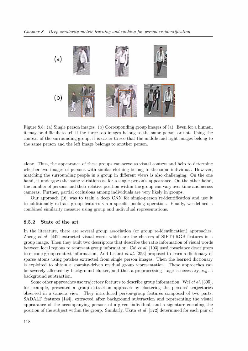
Chapter 8. Deep similarity metric learning and ranking for person re-identification
Figure 8.8: (a) Single person images. (b) Corresponding group images of (a). Even for a human,it may be difficult to tell if the three top images belong to the same person or not. Using thecontext of the surrounding group, it is easier to see that the middle and right images belong tothe same person and the left image belongs to another person.
alone. Thus, the appearance of these groups can serve as visual context and help to determinewhether two images of persons with similar clothing belong to the same individual. However,matching the surrounding people in a group in different views is also challenging. On the onehand, it undergoes the same variations as for a single person’s appearance. On the other hand,the number of persons and their relative position within the group can vary over time and acrosscameras. Further, partial occlusions among individuals are very likely in groups.
Our approach [16] was to train a deep CNN for single-person re-identification and use itto additionally extract group features via a specific pooling operation. Finally, we defined acombined similarity measure using group and individual representations.
8.5.2 State of the art
In the literature, there are several group association (or group re-identification) approaches.Zheng et al . [442] extracted visual words which are the clusters of SIFT+RGB features in agroup image. Then they built two descriptors that describe the ratio information of visual wordsbetween local regions to represent group information. Cai et al . [103] used covariance descriptorsto encode group context information. And Lisanti et al . [253] proposed to learn a dictionary ofsparse atoms using patches extracted from single person images. Then the learned dictionaryis exploited to obtain a sparsity-driven residual group representation. These approaches canbe severely affected by background clutter, and thus a preprocessing stage is necessary, e.g . abackground subtraction.
Some other approaches use trajectory features to describe group information. Wei et al . [395],for example, presented a group extraction approach by clustering the persons’ trajectoriesobserved in a camera view. They introduced person-group features composed of two parts:SADALF features [144], extracted after background subtraction and representing the visualappearance of the accompanying persons of a given individual, and a signature encoding theposition of the subject within the group. Similarly, Ukita et al . [372] determined for each pair of
118
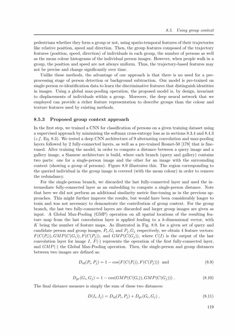
8.5. Using group context
pedestrians whether they form a group or not, using spatio-temporal features of their trajectorieslike relative position, speed and direction. Then, the group features composed of the trajectoryfeatures (position, speed, direction) of individuals in each group, the number of persons as wellas the mean colour histograms of the individual person images. However, when people walk in agroup, the position and speed are not always uniform. Thus, the trajectory-based features maynot be precise and change significantly over time.
Unlike these methods, the advantage of our approach is that there is no need for a pre-processing stage of person detection or background subtraction. Our model is pre-trained onsingle-person re-identification data to learn the discriminative features that distinguish identitiesin images. Using a global max-pooling operation, the proposed model is, by design, invariantto displacements of individuals within a group. Moreover, the deep neural network that weemployed can provide a richer feature representation to describe groups than the colour andtexture features used by existing methods.
8.5.3 Proposed group context approach
In the first step, we trained a CNN for classification of persons on a given training dataset usinga supervised approach by minimising the softmax cross-entropy loss as in sections 8.3.4 and 8.4.3(c.f . Eq. 8.3). We tested a deep CNN architecture of 9 alternating convolution and max-poolinglayers followed by 2 fully-connected layers, as well as a pre-trained Resnet-50 [178] that is fine-tuned. After training the model, in order to compute a distance between a query image and agallery image, a Siamese architecture is build, where each branch (query and gallery) containstwo parts: one for a single-person image and the other for an image with the surroundingcontext (showing a group of persons). Figure 8.9 illustrates this. The region corresponding tothe queried individual in the group image is covered (with the mean colour) in order to removethe redundancy.
For the single-person branch, we discarded the last fully-connected layer and used the in-termediate fully-connected layer as an embedding to compute a single-person distance. Notethat here we did not perform an additional similarity metric fine-tuning as in the previous ap-proaches. This might further improve the results, but would have been considerably longer totrain and was not necessary to demonstrate the contribution of group context. For the groupbranch, the last two fully-connected layers are discarded and larger group images are given asinput. A Global Max-Pooling (GMP) operation on all spatial locations of the resulting fea-ture map from the last convolution layer is applied leading to a k-dimensional vector, withK being the number of feature maps. As illustrated in Fig. 8.9, for a given set of query andcandidate person and group images, Pi, Gi and Pj, Gj respectively, we obtain 4 feature vectors:F (C(Pi)), GMP (C(Gi)), F (C(Pj)), and GMP (C(Gj)), where C(I) is the output of the lastconvolution layer for image I, F (·) represents the operation of the first fully-connected layer,and GMP (·) the Global Max-Pooling operation. Then, the single-person and group distancesbetween two images are defined as:
Did(Pi, Pj) = 1− cos(F (C(Pi)), F (C(Pj))) and (8.9)
Dgr(Gi, Gj) = 1− cos(GMP (C(Gi)), GMP (C(Gj))) . (8.10)
The final distance measure is simply the sum of these two distances:
D(Ii, Ij) = Did(Pi, Pj) +Dgr(Gi, Gj) , (8.11)
119

Chapter 8. Deep similarity metric learning and ranking for person re-identification
Figure 8.9: Overview of our group-assisted approach. Left: A CNN is first trained with single-person images. Right: For re-identification, the fully-connected layer(s) are removed and thesame CNN model is used for query and candidate images to compute pairwise distances usedfor the final ranking.
which can be used for ranking and for re-identification based on the first ranked result withrespect to a given query image.
8.5.4 Experiments
For evaluation our approach, we used the OGRE dataset [253], which contains 1 279 images of39 groups acquired by three disjoint cameras pointing at a parking lot. This is a challengingdataset with many different viewpoints and self-occlusions. We manually annotated a subset ofthis dataset with 450 bounding boxes and 75 identities.
To show that our approach can be applied with different CNN architectures, we used Resnet-50, pre-trained on ImageNet, and also our own CNN architecture (similar to the ones of theprevious sections and denoted as Convnet-5 here) composed of 9 alternating convolution andmax-pooling layers and 2 fully-connected layers.
The CMC scores (c.f . section 8.2.4) for person re-identification are shown in Table 8.7. Wecompared the person re-identification results with some variants of our method. “Sum feature”and “Concatenate feature” represent variants that first sum or concatenate the single-personfeature representation and the group feature representation and then compute the distancemeasure on these vectors. We tested also a variant that retains the query or candidate personimage in the group image without covering the corresponding region with the mean colour.
The results in Table 8.7 show that the proposed method (i.e. covering the person in thegroup image and summing the person and group distance) achieved the best re-identification
120
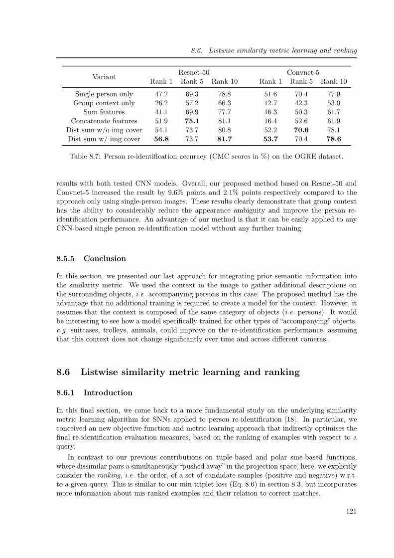
8.6. Listwise similarity metric learning and ranking
VariantResnet-50 Convnet-5
Rank 1 Rank 5 Rank 10 Rank 1 Rank 5 Rank 10
Single person only 47.2 69.3 78.8 51.6 70.4 77.9Group context only 26.2 57.2 66.3 12.7 42.3 53.0
Sum features 41.1 69.9 77.7 16.3 50.3 61.7Concatenate features 51.9 75.1 81.1 16.4 52.6 61.9
Dist sum w/o img cover 54.1 73.7 80.8 52.2 70.6 78.1Dist sum w/ img cover 56.8 73.7 81.7 53.7 70.4 78.6
Table 8.7: Person re-identification accuracy (CMC scores in %) on the OGRE dataset.
results with both tested CNN models. Overall, our proposed method based on Resnet-50 andConvnet-5 increased the result by 9.6% points and 2.1% points respectively compared to theapproach only using single-person images. These results clearly demonstrate that group contexthas the ability to considerably reduce the appearance ambiguity and improve the person re-identification performance. An advantage of our method is that it can be easily applied to anyCNN-based single person re-identification model without any further training.
8.5.5 Conclusion
In this section, we presented our last approach for integrating prior semantic information intothe similarity metric. We used the context in the image to gather additional descriptions onthe surrounding objects, i.e. accompanying persons in this case. The proposed method has theadvantage that no additional training is required to create a model for the context. However, itassumes that the context is composed of the same category of objects (i.e. persons). It wouldbe interesting to see how a model specifically trained for other types of “accompanying” objects,e.g . suitcases, trolleys, animals, could improve on the re-identification performance, assumingthat this context does not change significantly over time and across different cameras.
8.6 Listwise similarity metric learning and ranking
8.6.1 Introduction
In this final section, we come back to a more fundamental study on the underlying similaritymetric learning algorithm for SNNs applied to person re-identification [18]. In particular, weconceived an new objective function and metric learning approach that indirectly optimises thefinal re-identification evaluation measures, based on the ranking of examples with respect to aquery.
In contrast to our previous contributions on tuple-based and polar sine-based functions,where dissimilar pairs a simultaneously“pushed away” in the projection space, here, we explicitlyconsider the ranking, i.e. the order, of a set of candidate samples (positive and negative) w.r.t.to a given query. This is similar to our min-triplet loss (Eq. 8.6) in section 8.3, but incorporatesmore information about mis-ranked examples and their relation to correct matches.
121

Chapter 8. Deep similarity metric learning and ranking for person re-identification
8.6.2 State of the art
We already discussed the state of the art in similarity metric learning and SNN in section 7.2,and we will concentrate on approaches for ranking. In particular, we are interested here inone category of methods which is called learning-to-rank. This approach, widely applied ininformation retrieval and natural language processing, consists in learning a model that cancompute the optimal ordering of a list of items. Many learning-to-rank methods have beenproposed in the literature, like the pairwise approaches RankSVM [183], RankNet [100] andlistwise approaches ListNet [107], ListMLE [406] and LambdaRank [101], which take an entireranked list of objects as the learning instance.
Person re-identification could be considered as a retrieval problem based on ranking, wherethe matching images, i.e. the ones showing the same person as in the query image, should beranked before all the others. Some methods proposed in the literature follow this approach. Forexample, in the work of Prosser et al . [313] a set of weak RankSVMs is learnt, each computedon a small set of data, and then combined to build a stronger ranker using ensemble learning.Wang et al . [389] applied the ListMLE method to person re-identification: their approach mapsa list of similarity scores to a probability distribution, then utilizes the negative log likelihoodof ground truth permutations as the loss function.
8.6.3 Learning to rank with SNNs
The principal problem with rank learning with statistical machine learning approaches, partic-ularly neural networks, is that the rank is discrete, and, thus, rank errors are not differentiable.In order to apply an iterative gradient descent optimisation, the RankNet approach from Burgeset al . [100] uses a sigmoid function (which is convex and derivable) and pairwise relationships tomodel the ranking. Later, they proposed the LambdaRank method [101], where the gradient isscaled by the improvement of a global ranking measure (the Normalized Discounted CumulativeGain (NDCG)) incurred by swapping two examples in the ranking.
Our proposed approach is based on this approach. However, we do not use the pairwisecross-entropy loss function but the triplet loss (c.f . Eq. 7.7 in section 7.2.3). Also, we combinetwo ranking measures, the rank-1 (R1) score and the Average Precision (AP), i.e. the area underthe precision-recall curve, for a given query and ranking. Finally, we propose to minimise ourmodified triplet loss function, called Rank-Triplet, on batches of examples (i.e. lists), where, ineach batch, only the most relevant triplets are selected for updating the model parameters, i.e.we use only mis-ranked examples.
More precisely, a training batch is formed by M images of N identities. We take one examplein the batch as query and perform a ranking among the rest of images in the batch. (For thesake of a robust metric, we add a margin m to the distance of ranking positions between the truecorrespondences and the probe before ranking.) The AP and R1 scores are computed for eachof those query rankings. Then, with respect to one given query, we form all possible mis-rankedpairs (false correspondences ranked before the true correspondence), and we re-calculate the newAP and R1 scores by swapping positions of the pair in the ranking and thus obtain the gains∆AP and ∆R1, respectively. The loss of each triplet is weighted by the sum of these gains. The
122

8.6. Listwise similarity metric learning and ranking
Loss function R1 mAP
Classification loss 74.3 51.0Siamese loss 62.9 46.6Triplet loss 74.3 56.5
Quadruplet loss 74.9 58.1Hardbatch 81.0 63.9Baseline 82.1 66.5
Ours (Rank-triplet) 83.6 67.3
Table 8.8: Re-identification results (in %) on Market-1501 with different loss functions.
final Rank-triplet loss is calculated as follows:
Erank−triplet =1
MN
MN∑
i=1
1
Ki
∑
j∈TCi
∑
k∈FCi
rik<rij
[‖f(xi)− f(xj)‖22
− ‖f(xi)− f(xk)‖22+m] · (∆AP ijk +∆R1ijk), (8.12)
where xi is the ith training example in a training batch, Ki is the number of mis-ranked pairsw.r.t. the ith example as query, and rij is the rank of the jth example w.r.t. the ith image as
query. TCi/FCi is the true/false correspondence set of the ith example. ∆AP ijk is the gain of
AP by swapping the jth and kth examples w.r.t. the ith example as query and analogously forR1.
With our evaluation based weighting, we make a trade-off between the moderate hard ex-amples and hardest examples, i.e. more weight is given to the hardest examples to make thelearning efficient, and, at the same time, the less hard examples are used to stabilise the training.
8.6.4 Experiments
I will present here a summary of the results of our experiments on the person re-identificationproblem with a Resnet-50 neural network architecture pre-trained on Imagenet and with differentloss functions. More detailed experiments with different neural architectures and on an imageretrieval task can be found in [116].
First, we evaluated the re-identification performance of our Rank-Triplet approach on theMarket-1501 dataset and compared it with several other common loss functions. The resultsare shown in Table 8.8. For the supervised classification with identity labels, the softmax crossentropy loss is used. The margin in the Siamese loss and triplet loss is fixed to the default valuem = 1. For the pairwise Siamese learning the contrastive loss is used (c.f . Eq. 7.6), and wegenerated all possible pairs of images within a batch. The triplet loss is calculated accordingto Eq. 7.7. And the hard batch triplet loss takes only the hardest positive image and negativeimage, the hard batch triplet loss is calculated as follows.
Lhard−batch =1
N
N∑
i=1
max( maxj∈TCi
‖f(xi)− f(xj)‖22 − mink∈FCi)
‖f(xi)− f(xk)‖22+m, 0) , (8.13)
where N is the number of triplets, TCi/FCi is the true/false correspondence set of the ith
example.
123

Chapter 8. Deep similarity metric learning and ranking for person re-identification
MethodsMarket-1501 DukeMTMC-Reid CUHK03-NPR1 mAP R1 mAP R1 mAP
Hardbatch triplet loss [184] 81.0 63.9 62.8 42.7 46.4 50.6Our baseline 82.1 66.5 72.4 52.0 45.3 48.9
Our Rank-Triplet loss 83.6 67.3 74.3 55,6 47.8 52.4Rank-Triplet+re-rank [447] 86.2 79.8 78.6 71.4 60.4 60.8
LOMO+XQDA [250] 43.8 22.2 30.8 17.0 12.8 11.5LSRO [445] 78.1 56.2 67.7 47.1 - -
Divide and fuse [427] 82.3 72.4 - - 30.0 26.4K-reciprocal re-rank [447] 77.1 63.6 - - 34.7 37.4
ACRN[333] 83.6 62.6 72.6 52.0 - -SVDNet [361] 82.3 62.1 76.7 56.8 41.5 37.3JLML [248] 85.1 65.5 - - - -DPFL [115] 88.6 72.6 79.2 60.6 40.7 37.0
Table 8.9: Comparison of our Rank-Triplet approach with state-of-the-art methods for personre-identification.
The quadruplet loss in [113], based on triplets, pushes away also negative pairs from positivepairs w.r.t. different probe images. The loss is formulated as:
Equadruplet = −1
N
N∑
i=1
[max(‖f(xi)− f(xj)‖22−‖f(xi)− f(xk)‖22+m1, 0)
+max(‖f(xi)− f(xj)‖22−‖f(xk)− f(xl)‖22+m2, 0)], (8.14)
where xj is the feature embeddings of an image from the same identity as xi and xk,xl are fromdifferent identities. As [113], we set the m1 = 1,m2 = 0.5.
Finally, we implemented a baseline which is based on the Rank-triplet loss function withoutthe term for evaluation gain weighting. But the triplet selection is still based on the batchranking orders.
Our Rank-triplet achieved the best performance among these loss functions. This comparisonshows the effectiveness of the listwise evaluation measure-based weighting. Rank-triplet givesalso better results than hardbatch. This shows that using moderate difficult examples andweighting them helps the metric learning. Using the quadruplet loss also slightly improves theperformance with respect to triplets. This could eventually be combined with our loss.
We also compared our method with state-of-the-art methods on three benchmark datasets:Market-1501, DukeMTMC-Reid and CUHK03-NP. The results are shown in Table 8.9. Ourmethod Rank-triplet achieves better results than most of the other methods. Only on Market-1501, DPFL obtains a slightly better result, and SVDNet and DPFL on DukeMTMCReid. Onthe CUHK03 benchmark, our methods achieves the best results. DPFL and SVDNet are basedon a classification loss, and the CUHK03 dataset contains probably too few images per personto train a good classifier. However, the triplet loss is not much affected because a large numberof triplets can still be formed. Since the main contribution of these two state-or-the-art methodsfocuses on the network architecture, these methods can potentially be combined with our lossfunction.
124
8.7. Conclusion
8.6.5 Conclusion
In this section, we presented a final contribution on improving similarity metric learning withSNN-based models. This approach not only uses lists (or tuples) to improve the convergenceand final similarity metric, and thus the overall re-identification performance, but also directlyincorporates in the optimisation the order of the ranking of lists of examples (operating itera-tively on random batches). Our experimental results showed that this is a very powerful methodfor similarity metric learning on image-based recognition problems, like person re-identificationand image retrieval with challenging and realistic state-of-the-art datasets.
8.7 Conclusion
In summary, we presented four different approaches to improve similarity metric learning withSNNs illustrated on the (single-shot) person re-identification problem. We showed how semanticprior knowledge can be effectively incorporated in these neural network-based architectures,for example semantic pedestrian attributes and body orientation. Further, we presented anelegant approach to make use of scene context, i.e. surrounding persons, for re-identifying agiven person, which can be applied to any CNN-based person re-identification model withoutany further retraining and fine-tuning. Finally, we introduced an original objective function fora new learning-to-rank approach with SNNs giving state-of-the-art results.
Most of these contributions could be combined to probably further improve the results onperson re-identification. Also, applying some of these methods to the face and gesture verificationand classification problems of the previous chapter would be very interesting and give insightsinto the general performance of the different approaches. Despite the large progress that has beenrecently made on the person re-identification problem, there still remain some open issues thatmake their application to real-world settings difficult. For example, the overall generalisationcapacity of deep neural network models has been little studied in this context, because evaluationis usually conducted on a given test dataset that is similar to the training dataset in terms ofacquisition conditions. In real-world applications, methods that are performing well on any typeof realistic data are required, i.e. different viewing angles, resolution, lighting conditions, possiblyby new mechanisms that automatically adapt to new previously unseen environments (domainadaptation, unsupervised and continuous learning etc.). Further, the automatic optimal fusionof different cues would allow for more robust systems, e.g . the context of carried objects andaccompanying persons, the person’s gait, walking speed, characteristic motion as well as sceneinformation from several cameras, for example.
We will elaborate more on future research directions in the following section.
125

Chapter 8. Deep similarity metric learning and ranking for person re-identification
126

9 Conclusion and perspectives
In the preceding chapters, I described a large part of our research work that I co-supervised andthat I was involved in during the last 10 years. I had the chance the work in several Europeancountries with extremely competent persons and on a variety of related topics, which, on the onehand, gave me a solid technical and scientific background, and on the other hand, broadenedand enriched my culture, vision and thinking in various aspects.
Of course, this is not an exhaustive report of all the work that I have been involved in. Onlythe most representative results are presented, and I have not mentioned some of the more recentstudies. For example, our work on weakly supervised and unsupervised learning techniques forobject recognition and tracking, performed in a lab-internal project across several teams andwith two Master students. And also, our work on neural network compression and approximationconducted within the context of an international collaboration with a colleague from the FederalPernambuco University, Recife, Brazil. I will briefly describe these in the perspectives, as bothof the studies are being pursued, or will be, with PhD theses starting in 2018 and 2019.
But before outlining future research directions and projects, I will first summarise the re-search work that I presented in this manuscript and draw some general conclusions.
9.1 Summary of research work and general conclusion
Although there is some overlap, I categorised the description of our past research into two parts,mainly due to the context of the two different research institutes and environments I have beenworking in: Idiap and LIRIS. The first part described our machine learning and computer visionapproaches for visual object tracking in challenging dynamic environments, and the secondoutlined our contributions on weakly-supervised metric learning methods using Siamese NeuralNetworks.
From a computer vision point of view, we first focused on on-line multiple object trackingin videos from a single RGB camera, and in particular, multiple face tracking applications indynamic contexts, and we addressed a variety of common problems, such as data association,the tracking of a variable number of objects, an efficient inference for real-time applications, theintegration and adaptation of robust appearance models.
In particular, in chapter 5, we proposed an effective on-line algorithm for multi-face trackingthat is able to cope with missing face detections over longer periods of time without losingthe object, as well as frequent false detections without falsely initialising new tracks. Then, weextended this work by an additional algorithm that estimates the Visual Focus of Attention ofa tracked person. The proposed unsupervised on-line learning approach learns a robust modelfrom very few examples of face images acquired during the tracking.
In chapter 6, we limited ourselves on tracking a single object in a video and focused oncreating more robust appearance models and on-line learning approaches. This included three
127
Chapter 9. Conclusion and perspectives
major contributions: one method particularly suited to tracking deformable objects in challeng-ing videos without any prior knowledge, another method including motion context in the on-linelearning of a robust discriminative appearance model and the last contribution resulting fromthe PhD work with Salma Moujtahid [? ] proposing a method that effectively and dynam-ically incorporates the scene context in the tracking process by selecting tracking algorithmsspecialised for a given environment and context.
In the second part, in chapter 7, I presented our work with Lilei Zheng [441] and SamuelBerlemont [90] on Siamese Neural Networks for similarity metric learning, applied to pairwiseface verification as well as gesture and action classification. Through more balanced and betterconditioned objective functions and learning algorithms, our proposed approaches were able toaddress several problems, such as the better rejection of unknown classes and a higher classifi-cation and verification performance.
In the final chapter, in the context of the PhD thesis of Yiqiang Chen [116], we studiednon-linear similarity metric learning approaches employing more complex SNN models based ondeeper CNN architectures. Our work focused here on the application of person re-identificationin images coming from several cameras with non-overlapping views. We showed that the useof pedestrian attributes in the learnt similarity metric, and different models that are specific todifferent body orientations as well as person group context largely improves the re-identificationperformance.
From a machine learning point of view, in the presented work in the first part, one cannotice a trend from off-line learnt models (e.g . for track creation and removal) to more on-linelearning (e.g . for the objects’ appearance). There is a natural need for such algorithms in on-line visual tracking approaches, and on-line data processing methods in general. However, thereis a considerable risk of model drift because very few training data is usually available, andthe model needs to be adapted continuously to changes of the object or environment without“forgetting” previously acquired relevant information (the “stability-plasticity” dilemma). Toaddress this problem, we first proposed an effective on-line learnt model for pixel-wise detectionand segmentation and a co-training framework, where the estimation of one model (detector) isused to update the model of the other one (segmentation) (and vice versa). And in the work onscene context, this idea is extended to several models, where only the selected model updates allthe other ones at each point in time. Nevertheless, more principled methods for on-line learning(with neural networks) and the better integration and understanding of contextual informationare still needed.
Another trend of the presented work is from supervised learning used for MOT, to algorithmsthat are only weakly supervised, which we have employed for the similarity metric learning withSNNs. We have presented several new objective functions (tuple-based, polar sine-based, Rank-triplet etc.) and example selection strategies that improved the training and the performanceof SNNs for various different applications. We further introduced original neural architecturesand training strategies that allowed us to introduce semantic external knowledge. In this way,we were able to combine different models that have been trained in a supervised and weaklysupervised way, according to the quantity of data as well as the quantity and type of annotationthat is available.
To summarise, we made several significant contributions in visual object tracking to improvethe long-term performance and to improve the robustness of the visual appearance models andon-line learning. Nevertheless, many challenges still remain. Several recent tracking methodsare based on deep CNNs and showed excellent performance on public benchmarks. However,there are two major issues to be considered. First, these models cannot be created from very fewtraining data as in short video sequences. Thus, they need to be pre-trained on large datasets
128

9.2. Perspectives
such as ImageNet and “fine-tuned” on-line on a given test video. This pre-training introducesa large bias on the type of videos and the type of objects to be tracked. Also, the on-linelearning or fine-tuning of neural networks with such non-stationary data is a topic that has notbeen studied much in machine learning. We will come back to this issue in the perspectives.The second issue is the computational complexity of deep CNNs. Apparently, such modelscan operate in real-time with recent GPUs. But, the memory requirements and especially thepower consumption make their usage mostly impossible or at least impractical for smaller-scalehardware, such as embedded systems. We will also come back to this in the perspectives.
Concerning similarity metric learning, we made several important contributions to improvetheir convergence and performance of SNNs for verification, classification and ranking, both onthe theoretical and practical side. With the current revival and exaltation for neural networks,there has been some recent work and advances on metric learning with deep neural networksand deep CNN (as ours in chapter 8). However, as some of these models are very complex andrequire a significant amount of training data, some fundamental questions arise. For example,how generic is the learnt similarity metric, i.e. how does it cope with unseen data? Accordingto some of our experiments with large amounts of training data, the difference in classificationperformance between a supervised and a weakly supervised model seems to decrease. This maysuggest that the learnt metric just “compares” the given test data to the learnt examples bycomputing a type of non-linear distance, which might give very poor results when the test datadistribution is too far from the training data. We will further investigate these phenomena in ourfuture work. In any case, the inclusion of prior knowledge into the metric learning showed to bea very effective approach. We showed that external semantic information improves the overallperformance, but as labels may not be available abundantly it would also be interesting, in thefuture, to investigate how unsupervised learning may help the metric learning. This may alsobe used to better define or learn the somewhat vague notions of “similarity” and “dissimilarity”imposed by traditional SNN approaches.
9.2 Perspectives
There are numerous perspectives and possible future directions for our research, and, in thefollowing, I will present the most important ones. My colleagues and I have the chance to haveobtained the funding for several PhD students that will start soon or have started recently andthat will give us the opportunity to do research on these topics. I will co-supervise them withmy colleagues from LIRIS and other laboratories, which will further allow me to strengthenexisting collaborations within and between different teams (“Imagine”, “Data Mining and Ma-chine Learning” (DM2L) and “Multi-Agent Systems” (SMA)) and start new collaborations withothers (Laboratoire Hubert Curien (LHC), Saint Etienne, ENS Lyon, UCLy). This evolution interms of funding and new supervision activities as well as the identified new research directionsoutlined in the following give me a strong motivation for my habilitation and to build up myown research group.
More specifically, the following topics will be the focus of my research for the next 4–6 years.
9.2.1 On-line and sequential similarity metric learning
In 2018, Christophe Garcia and I continued our collaboration with Gregoire Lefebvre at OrangeLabs, Grenoble, related to the work that has been carried out during the PhD thesis of SamuelBerlemont (c.f . chapter 7). Within the context of a newly funded PhD, being performed byPaul Compagnon, we will explore and develop new methods and techniques for SNN-based
129

Chapter 9. Conclusion and perspectives
similarity metric learning of temporal sequences of mobile sensor data. The goal here is todiscover and recognise patterns and routines, for example of elderly persons, using inertial sensordata, e.g . from a mobile phone, a smart watch etc. To this end, we will study new approachesbased on recurrent SNNs and on unsupervised and weakly supervised learning that will allow toautomatically recognise similar patterns that are recurring and others that are more exceptionalor abnormal in order to detect when there is a degradation in the autonomy or any other problemrelated to the health of the person. Very little work has been done so far on such recurrent SNN-based similarity metric learning approaches to characterise and classify sequential data.
Another work on metric learning on images has started with the PhD that I am co-supervisingwith Christophe Garcia and Pierre Letissier from the “Institut National de l’Audiovisuel” (INA)in Paris. In this upcoming work that will be conducted by Thomas Petit, we will study newapproaches based on deep convolutional SNN for the indexation of videos and broadcasts byrecognising faces in large-scale face image datasets. A part from the large training data volume,we will focus on two scientific aspects here. First, we will investigate how such a complex SNNsimilarity metric can generalise to unseen faces, and how it can effectively and incrementallylearn from sequential streams of (face) data and user annotation. And second, we will seekto develop new compressed, robust representations of faces (particular embeddings, hash codesetc.) to allow for an efficient indexation and retrieval of images and videos containing faces orpossibly other specific content.
9.2.2 Autonomous developmental learning for intelligent vision
During the last two years, in a lab-internal project between the teams Imagine (ChristopheGarcia and myself, INSA Lyon) and SMA (Frederic Armetta, Mathieu Lefort, University Lyon1), we conducted exploratory research on new approaches for learning visual representation torecognise and track objects in videos in a completely unsupervised way and with minimum priorknowledge. Two Master students supported us on this ambitious project, and we were ableto develop some novel ideas and approaches [19] based on developmental and constructivistlearning and SNNs. Figure 9.1 illustrates the principle procedure. Given a video stream, a firstalgorithm detects salient image regions in each frame based on low-level visual features (colour,edges, motion etc.). Then, using temporal consistent pairs of detected image regions, visualrepresentations of candidate objects are learnt on-line with a Siamese CNN architecture. Theoutput of the neural network forms an embedding space where similar objects are close anddifferent objects further apart. After a bootstrapping learning phase, this learnt model can inturn be used to better detect and recognise the objects in the scene. To improve the embeddingand the convergence, we extended this approach with multi-task learning of image reconstructionand object segmentation and with an attention mechanism that focuses on different objects inthe scene over time.
Many challenges and open issues remain in this project: for example, how to learn incremen-tally and update an optimal representation from a continuous stream of (visual) data withoutany prior knowledge, what are the perception, attention and memory mechanisms that allowfor plastic and abstract representations that are efficient for recognising known objects and fortransferring learnt knowledge to unknown environments, and how can higher-level informationbe integrated in the model and be used to help this autonomous process, e.g . the scene con-text, higher-level temporal or causal information, sensori-motor stimuli, affordances etc. Thesefundamental issues will be studied in the context of the PhD thesis of Ruiqi Dai, that I will co-supervise with my colleagues from the SMA team and a researcher in humanities (philosophy),Matthieu Guillermin from the “Institut Catholique de Lyon”.
130

9.2. Perspectives
Figure 9.1: Our autonomous perceptive learning approach.
9.2.3 Neural network model compression
With the advent of General-Purpose GPU computing and large-scale High-Performance Com-puting (HPC) applied to CNNs, more and more complex, deep neural network models have beendeveloped requiring large amounts of computational and memory resources for training and in-ference. However, it has been shown that the redundancy in such models is very large, and thatthey can be reduced in size by several orders of magnitude using specific quantisation, factori-sation or pruning techniques without any major negative impact on the overall (classification)performance.
In our recent collaboration with Renato Cintra and Andre Leite from the Federal Pernam-buco University, Recife, Brazil, we proposed an approach that approximates the parameters of atrained neural network with so-called dyadic rationals, i.e. powers of two, and Canonical SignedDigit-coded factors. In this way, we were able to obtain multiplication-free approximations of themodels, i.e. requiring only bit shifts and additions, paving the way for very low-complexity hard-ware implementations of deep neural networks. We showed the effectiveness of our approach [1]on a variety of tasks and network architectures, MLPs and CNNs, including the well-knownAlexNet trained on ImageNet [220].
This is an exciting research area that we will continue to explore. It raises also some fun-damental questions and issues that we will tackle in the near future. For example, instead ofreducing the complexity of already trained neural networks, can we develop an algorithm thatdirectly learns such sparse or simplified models while maintaining the same classification per-formance? In a PhD thesis starting soon in the context of an ambitious research project called“Academics” between LIRIS, LHC, LIP and the Physics Laboratory of ENS Lyon and funded by
131

Chapter 9. Conclusion and perspectives
the IDEX Lyon Scientific Breakthrough program, we will investigate new approaches to learnsparse neural networks applied to large-scale problems related to complex dynamical systems(e.g . climate models, social networks). To this end, with my colleagues from the DM2L team,Marc Plantevit and Celine Robardet, we will work on the combination of specific data miningand feature selection methods to reduce the noise and redundancy in the training data as wellas in the model. In particular, we will try to identify frequent and typical activation patternsof a trained neural network graph, layer-wise and across several layers, in order to remove (i.e.prune) redundant or useless neurons and to understand the responsibilities of different parts ofthe model that we will then try to factorise and combine. A preliminary study (Master thesis)on this topic gave promising experimental results.
We will also investigate methods for building simpler and more sparse models directly duringtraining. Recently, approaches that construct neural network architectures that incrementallyand iteratively grow (e.g . Neural Architecture Search, Network Morphism) may provide aninteresting starting point.
In the PhD thesis of Guillaume Anoufa on far-field object detection and recognition invideo streams that will in 2019 and that I will co-supervise with Christophe Garcia and Nico-las Belanger from Airbus Helicopters, we will also tackle this problem of model simplificationand compression with CNNs. We will approach this from the training data side and withsemi-supervised learning, i.e. we will create synthetic annotated images for training a classifier.Among other issues, we will investigate how the choice and type of synthetic data influences theperformance and capability to automatically build a neural model of reduced size and complexityand increased generalisation capacity.
9.2.4 From deep learning to deep understanding
Exploring and developing new learning strategies and neural network architectures, possiblyin a self-organising and autonomous way, may provide numerous further perspectives. First,drastically reducing the computational complexity and memory requirements of deep neuralnetworks will not only allow for a efficient deployment in embedded devices (the Internet ofThings) giving them increased AI capabilities but also enable powerful machine learning-basedmodelling of complex large-scale problems such as climate and weather prediction in physics orbrain signal analysis and interpretation in Neuroscience.
Another issue that gains increasing interest in the AI and Machine Learning research com-munities is the fact that trained deep neural network models and their inference are difficultto interpret and explain for humans, which leads to an increasing interest in “Explainable AI”approaches. Much work is still to be done to introduce this “explainability”and“interpretability”into neural network-based models, and this will be one perspective of our future work on modelsimplification and sparsity. That is, we will seek to learn models that favour the identificationand isolation of processing paths or sub-models allowing to more easily incorporate and learnsemantic knowledge, probably of symbolic nature. This may also raise and hopefully answersome questions on causality. The goal here is formally and statistically analyse input-outputcorrelations at different levels of the trained model, and, further, to develop new training strate-gies that specifically create such correlations favouring explainable representations, functionsand processing paths.
The automatic learning of higher-level concepts, and the effective mechanisms of storing,processing, and transforming them clearly forms the foundation of a strong AI that is able tomemorise, recognise and to reason. I believe that much work has still to be done in this regard,and that this can only be achieved in a multi-disciplinary approach involving researchers from AI,
132

9.2. Perspectives
Machine Learning, Robotics, Computer Vision, Cognitive Science and Psychology, Neuroscience,Physics and Mathematics among others. I am keen to accept this challenge in the future, and,in the long term, I hope that we will not only be able to make significant progress towards ageneral AI but, more importantly, that these results will help us to better understand humanintelligence and the human brain as well as the world that surrounds us.
133

Chapter 9. Conclusion and perspectives
134
Publications
Journals
[1] Renato J. Cintra, Stefan Duffner, Christophe Garcia, and Andre Leite. Low-complexityapproximate Convolutional Neural Networks. IEEE Transactions on Neural Networks andLearning Systems, March 2018.
[2] Samuel Berlemont, Gregoire Lefebvre, Stefan Duffner, and Christophe Garcia. Class-balanced siamese neural networks. Neurocomputing, 273:47–56, 2018.
[3] Yiqiang Chen, Stefan Duffner, Andrei Stoian, Jean-Yves Dufour, and Atilla Baskurt. Deepand low-level feature-based attribute learning for person re-identification. In Image andVision Computing, 2018.
[4] Lilei Zheng, Stefan Duffner, Khalid Idrissi, Christophe Garcia, and Atilla Baskurt. Pair-wise identity verification via linear concentrative metric learning. IEEE Transactions onCybernetics, 48(1):324–335, 2018.
[5] Stefan Duffner and Christophe Garcia. Fast pixelwise adaptive visual tracking of non-rigidobjects. IEEE Transactions on Image Processing, 26(5):2368–2380, 2017.
[6] S. Duffner and C. Garcia. Using discriminative motion context for on-line visual objecttracking. IEEE Transactions on Circuits and Systems for Video Technology, 26(12):2215–2225, 2016.
[7] S. Duffner and C. Garcia. Visual focus of attention estimation with unsupervised in-cremental learning. IEEE Transactions on Circuits and Systems for Video Technology,26(12):2264–2272, 2016.
[8] Lilei Zheng, Stefan Duffner, Khalid Idrissi, Christophe Garcia, and Atilla Baskurt. SiameseMulti-layer Perceptrons for dimensionality reduction and face identification. MultimediaTools and Applications, 75(9):5055–5073, 2016.
[9] T. Nakashika, T. Yoshioka, T. Takiguchi, Y. Ariki, S. Duffner, and C. Garcia. ConvolutiveBottleneck Network with Dropout for Dysarthric Speech Recognition. Transactions onMachine Learning and Artificial Intelligence, pages 1–15, April 2014.
[10] S. Duffner, C. Liu, and J.-M. Odobez. Leveraging colour segmentation for upper-bodydetection. Pattern Recognition, 47(6):2222–2230, 2014.
[11] P. Motlicek, S. Duffner, D. Korchagin, H. Bourlard, C. Scheffler, J.-M. Odobez, O. Thier-gart, G. Del Galdo, and F. Kuech. Real-time audio-visual analysis for multiperson video-conferencing. Advances in Multimedia, 2013, August 2013.
135

Publications
[12] S. Duffner and Jean-Marc Odobez. A track creation and deletion framework for long-termonline multi-face tracking. IEEE Transactions on Image Processing, 22(1):272–285, 2013.
[13] S. Duffner, P. Motlicek, and D. Korchagin. The TA2 database – a multi-modal databasefrom home entertainment. International Journal of Computer and Electrical Engineering,4(5):670–673, 2012.
[14] A. Herbulot, S. Jehan-Besson, S. Duffner, M. Barlaud, and G. Aubert. Segmentationof vectorial image features using shape gradients and information measures. Journal ofMathematical Imaging and Vision, 25(3):365–386, October 2006.
International Conferences and Workshops
[15] Yiqiang Chen, Stefan Duffner, Andrei Stoian, Jean-Yves Dufour, and Atilla Baskurt.Pedestrian attribute recognition with part-based CNN and combined feature represen-tations. In Proceedings of the International Conference on Computer Vision Theory andApplications (VISAPP), Funchal, Portugal, January 2018.
[16] Yiqiang Chen, Stefan Duffner, Andrei Stoian, Jean-Yves Dufour, and Atilla Baskurt. Per-son re-identification using group context. In Proceedings of the International Conferenceon Advanced Concepts for Intelligent Vision Systems (ACIVS), 2018.
[17] Yiqiang Chen, Stefan Duffner, Andrei Stoian, Jean-Yves Dufour, and Atilla Baskurt. Per-son re-identification with a body orientation-specific convolutional neural network. InProceedings of the International Conference on Advanced Concepts for Intelligent VisionSystems (ACIVS), 2018.
[18] Yiqiang Chen, Stefan Duffner, Andrei Stoian, Jean-Yves Dufour, and Atilla Baskurt. Sim-ilarity learning with listwise ranking for person re-identification. In Proceedings of theInternational Conference on Image Processing (ICIP), 2018.
[19] Nawel Medjkoune, Frederic Armetta, Mathieu Lefort, and Stefan Duffner. Autonomousobject recognition in videos using siamese neural networks. In EUCognition Meeting (Euro-pean Society for Cognitive Systems) on ”Learning: Beyond Deep Neural Networks”, Zurich,Switzerland, November 2017.
[20] Yiqiang Chen, Stefan Duffner, Andrei Stoian, Jean-Yves Dufour, and Atilla Baskurt.Triplet CNN and pedestrian attribute recognition for improved person re-identification. InProceedings of the International Conference on Advanced Video and Signal-Based Surveil-lance (AVSS), Lecce, Italy, August 2017.
[21] Smrity Bhattarai, Arjuna Madanayake, Renato J. Cintra, Stefan Duffner, and ChristopheGarcia. Digital architecture for real-time CNN-based face detection for video process-ing. In IEEE Cognitive Communications for Aerospace Applications Workshop (CCAA),Cleveland, USA, June 2017.
[22] Samuel Berlemont, Gregoire Lefebvre, Stefan Duffner, and Christophe Garcia. Polar sinebased siamese neural network for gesture recognition. In Proceedings of the Interna-tional Conference on International Conference on Artificial Neural Networks (ICANN),Barcelona, Spain, 2016.
136

[23] Matej Kristan, Jiri Matas, Ales Leonardis, Michael Felsberg, Luka Cehovin, GustavoFernandez, Tomas Vojir, Gustav Hager, Georg Nebehay, Roman Pflugfelder, and Ste-fan Duffner et al. The Visual Object Tracking VOT2015 challenge results. In ICCV(Workshop), December 2015.
[24] Samuel Berlemont, Gregoire Lefebvre, Stefan Duffner, and Christophe Garcia. Siameseneural network based similarity metric for inertial gesture classification and rejection. InProceedings of the International Conference on Automatic Face and Gesture Recognition(FG), Ljubljana, Slovenia, May 2015.
[25] Jiwen Lu, Junlin Hu, Venice Erin Liong, Xiuzhuang Zhou, Andrea Bottino, Ihtesham UlIslam, Tiago Figueiredo Vieira, Xiaoqian Qin, Xiaoyang Tan, Songcan Chen, Yosi Keller,Shahar Mahpod, Lilei Zheng, Khalid Idrissi, Christophe Garcia, Stefan Duffner, AtillaBaskurt, Modesto Castrillon-Santana, and Javier Lorenzo-Navarro. The FG 2015 KinshipVerification in the Wild Evaluation. In Proceedings of the International Conference onAutomatic Face and Gesture Recognition (FG), Ljubljana, Slovenia, May 2015.
[26] Lilei Zheng, Khalid Idrissi, Christophe Garcia, Stefan Duffner, and Atilla Baskurt. Tri-angular similarity metric learning for face verification. In Proceedings of the InternationalConference on Automatic Face and Gesture Recognition (FG), Ljubljana, Slovenia, May2015.
[27] Lilei Zheng, Khalid Idrissi, Christophe Garcia, Stefan Duffner, and Atilla Baskurt. Logisticsimilarity metric learning for face verification. In Proceedings of the International Confer-ence on International Conference on Acoustics, Speech, and Signal Processing (ICASSP),April 2015.
[28] Salma Moujtahid, Stefan Duffner, and Atilla Baskurt. Classifying global scene context foron-line multiple tracker selection. In Proceedings of the British Machine Vision Conference(BMVC), 2015.
[29] Salma Moujtahid, Stefan Duffner, and Atilla Baskurt. Coherent selection of independenttrackers for real-time object tracking. In Proceedings of the International Conference onComputer Vision Theory and Applications (VISAPP), 2015.
[30] Toru Nakashika, Toshiya Yoshioka, Tetsuya Takiguchi, Yasuo Ariki, Stefan Duffner, andChristophe Garcia. Dysarthric speech recognition using a convolutive bottleneck network.In IEEE International Conference on Signal Processing (ICSP), pages 505–509, October2014.
[31] S. Duffner and C. Garcia. Exploiting contextual motion cues for visual object tracking. InWorkshop on Visual Object Tracking Challenge (VOT2014) - ECCV, pages 1–12, Septem-ber 2014.
[32] Matej Kristan, Roman Pflugfelder, Ales Leonardis, Jiri Matas, Luka Cehovin, Georg Nebe-hay, Tomas Vojir, Gustavo Fernandez, and Stefan Duffner et al. The Visual ObjectTracking VOT2014 challenge results. In Workshop on Visual Object Tracking Challenge(VOT2014) - ECCV, LNCS, pages 1–27, September 2014.
[33] S. Duffner, S. Berlemont, G. Lefebvre, and C. Garcia. 3D gesture classification with convo-lutional neural networks. In Proceedings of the International Conference on InternationalConference on Acoustics, Speech, and Signal Processing (ICASSP), May 2014.
137

Publications
[34] S. Duffner and C. Garcia. Pixeltrack: a fast adaptive algorithm for tracking non-rigidobjects. In Proceedings of the International Conference on International Conference onComputer Vision (ICCV), Sidney, AUS, December 2013.
[35] S. Duffner and C. Garcia. Unsupervised online learning of visual focus of attention. In Pro-ceedings of the International Conference on Advanced Video and Signal-Based Surveillance(AVSS), Krakow, PL, August 2013.
[36] D. Korchagin, S. Duffner, P. Motlicek, and C. Scheffler. Multimodal cue detection en-gine for orchestrated entertainment. In Proceedings of the International Conference onMultiMedia Modeling, Klagenfurt, Austria, January 2012.
[37] D. Korchagin, P. Motlicek, and S. Duffner. Just-in-time multimodal association and fusionfrom home entertainment. In IEEE International Conference on Multimedia and Expo(ICME), Workshop on Multimodal Audio-based Multimedia Content Analysis (MAMCA),Barcelone, Espagne, July 2011.
[38] S. Duffner and Jean-Marc Odobez. Exploiting long-term observations for track creationand deletion in online multi-face tracking. In Proceedings of the International Conferenceon Automatic Face and Gesture Recognition (FG), Santa Barbara, USA, March 2011.
[39] S. Duffner, D. Korchagin, and P. Motlicek. The TA2 database - a multi-modal databasefrom home entertainment. In International Conference on Signal Acquisition and Process-ing (ICSAP), Singapour, February 2011.
[40] S. Duffner, J.-M. Odobez, and E. Ricci. Dynamic partitioned sampling for tracking withdiscriminative features. In Proceedings of the British Machine Vision Conference (BMVC),London, UK, September 2009.
[41] S. Duffner and C. Garcia. Robust face alignment using convolutional neural networks. InProceedings of the International Conference on Computer Vision Theory and Applications(VISAPP), Funchal, Portugal, January 2008.
[42] S. Duffner and C. Garcia. Face recognition using non-linear image reconstruction. In Pro-ceedings of the International Conference on Advanced Video and Signal-Based Surveillance(AVSS), pages 459–464, London, UK, September 2007.
[43] S. Duffner and C. Garcia. An online backpropagation algorithm with validation error-based adaptive learning rate. In Proceedings of the International Conference on ArtificialNeural Networks (ICANN), volume 1, pages 249–258, Porto, Portugal, September 2007.
[44] S. Roux, F. Mamalet, C. Garcia, and S. Duffner. An embedded robust facial featuredetector. In International Conference on Machine Learning and Signal Processing (MLSP),pages 170–175, Thessaloniki, Greece, August 2007.
[45] C. Garcia and S Duffner. Facial image processing with convolutional neural networks.In International Workshop on Advances in Pattern Recognition (IWAPR), pages 97–108,Plymouth, United Kingdom, July 2007.
[46] S. Duffner and C. Garcia. A neural scheme for robust detection of transparent logos in TVprograms. In Proceedings of the International Conference on Artificial Neural Networks(ICANN), volume 2, pages 14–23, Athens, Greece, September 2006.
138

[47] S. Duffner and C. Garcia. A connexionist approach for robust and precise facial featuredetection in complex scenes. In Fourth International Symposium on Image and SignalProcessing and Analysis (ISPA), pages 316–321, Zagreb, Croatia, September 2005.
National Conferences
[48] Yiqiang Chen, Stefan Duffner, Andrei Stoian, Jean-Yves Dufour, and Atilla Baskurt. Re-identification de personne avec perte min-triplet. In 16e journees francophones des jeuneschercheurs en vision par ordinateur, Colleville-sur-mer, France, June 2017.
[49] A. Lehuger, S. Duffner, and C. Garcia. A robust method for automatic player detectionin sport videos. In Compression et Representation des Signaux Audiovisuels (CORESA),Montpellier, France, November 2007.
[50] S. Duffner and C. Garcia. A hierarchical approach for precise facial feature detection.In Compression et Representation des Signaux Audiovisuels (CORESA), pages 29–34,Rennes, France, November 2005.
[51] S. Jehan-Besson, S. Duffner, A. Herbulot, M. Barlaud, and Aubert G. Utilisation desgradients de forme et des contours actifs bases regions pour la segmentation des vecteursmouvement. In GRETSI, Louvain la Neuve, Belgique, September 2005.
Book Chapters
[52] M. Everingham, A. Zisserman, C. K. I. Williams, L. Van Gool, A. Moray, C. M. Bishop,O. Chapelle, N. Dalal, T. Deselaers, G. Dorko, S. Duffner, J. Eichhorn, J. D. R. Far-quhar, M. Fritz, C. Garcia, T. Griffiths, F. Jurie, T. Keysers, M. Koskela, J. Laaksonen,D. Larlus, B. Leibe, H. Meng, H. Ney, B. Schiele, C. Schmid, E. Seemann, J. Shawe-Taylor, A. Storkey, S. Szedmak, B. Triggs, I. Ulusoy, V. Viitaniemi, , and J. Zhang. The2005 PASCAL Visual Object Classes Challenge, Selected Proceedings of the first PASCALChallenges Workshop. Lecture Notes in Artificial Intelligence, Springer, 2006.
Patents
[53] C. Garcia and S. Duffner. Procede de recadrage d’images de visage”, FR20060053734,WO2007FR51900. 2006.
[54] C. Garcia and S. Duffner. Procede de reconnaissance de visages par reconstruction croiseenon lineaire FR20060055929, WO2007FR52569. 2006.
[55] C. Garcia and S. Duffner. Systeme et procede de localisation de points d’interet dans uneimage d’objet mettant en œuvre un reseau de neurones, FR20050003177, US20060910159,WO2006EP61110. 2005.
139

Publications
Other
[56] S. Duffner. Face Image Analysis With Convolutional Neural Networks. PhD thesis, Albert-Ludwigs-Universitat Freiburg im Breisgau, Freiburg im Breisgau, Germany, 2007.
[57] S. Duffner. Spatio-temporal segmentation of moving objects in image sequences. Master’sthesis, Ecole Nationale Superieure d’Ingenieurs de Caen (ENSICAEN), Caen, France, 2004.
140

Bibliography
[58] A. Adam, E. Rivlin, and I. Shimshoni. Robust fragments-based tracking using the integralhistogram. In Proceedings of the IEEE International Conference on Computer Vision andPattern Recognition (CVPR), pages 798–805, June 2006.
[59] A. Adam, E. Rivlin, and I. Shimshoni. Robust fragments-based tracking using the integralhistogram. In Proceedings of the International Conference on Computer Vision and PatternRecognition (CVPR), pages 798–805, 2006.
[60] Chad Aeschliman, Johnny Park, and Avinash C. Kak. A probabilistic framework for jointsegmentation and tracking. In Proceedings of the International Conference on ComputerVision and Pattern Recognition (CVPR), pages 1371–1378, June 2010.
[61] Ejaz Ahmed, Michael Jones, and Tim KMarks. An improved deep learning architecture forperson re-identification. In Proceedings of the IEEE International Conference on ComputerVision and Pattern Recognition (CVPR), pages 3908–3916, 2015.
[62] T. Ahonen, A. Hadid, and M. Pietikainen. Face recognition with local binary patterns.In Proceedings of the European Conference on Computer Vision (ECCV), pages 469–481.Springer, 2004.
[63] O. Akin, E. Erdem, A. Erdem, and K. Mikolajczyk. Deformable part-based tracking bycoupled global and local correlation filters. Journal of Visual Communication and ImageRepresentation, 38:763–774, 2016.
[64] A. Akl and S. Valaee. Accelerometer-based gesture recognition via dynamic-time warping,affinity propagation, & compressive sensing. In Proceedings of the International Conferenceon Acoustics, Speech, and Signal Processing (ICASSP), 2010.
[65] S. R. Arashloo and J. Kittler. Efficient processing of MRFs for unconstrained-pose facerecognition. In Biometrics: Theory, Applications and Systems (BTAS), pages 1–8. IEEE,2013.
[66] Shervin Rahimzadeh Arashloo and Josef Kittler. Class-specific kernel fusion of multipledescriptors for face verification using multiscale binarised statistical image features. IEEETransactions on Information Forensics and Security, 9(12):2100–2109, 2014.
[67] Stylianos Asteriadis, Kostas Karpouzis, and Stefanos Kollias. Visual focus of attentionin non-calibrated environments using gaze estimation. International Journal of ComputerVision, 107(3):293–316, 2013.
[68] Shai Avidan. Ensemble tracking. IEEE Transactions on Pattern Analysis and MachineIntelligence, 29(2):261–271, February 2007.
141
Bibliography
[69] Sileye O. Ba and Jean-Marc Odobez. A Rao-Blackwellized mixed state particle filter forhead pose tracking. In Proceedings of ICMI Workshop on Multi-modal Multi-party MeetingProcessing (MMMP), pages 9–16, 2005.
[70] Sileye O. Ba and Jean-Marc Odobez. Evaluation of multiple cue head pose estimationalgorithms in natural environements. In Proceedings of ICME, pages 1330–1333, 2005.
[71] Sileye O. Ba and Jean-Marc Odobez. Recognizing visual focus of attention from headpose in natural meetings. IEEE Transactions on Systems, Man, and Cybernetics. Part B,Cybernetics, 39(1):16–33, February 2009.
[72] Sileye O. Ba and Jean-Marc Odobez. Multiperson visual focus of attention from headpose and meeting contextual cues. IEEE Transactions on Pattern Analysis and MachineIntelligence, 33(1):101–116, 2011.
[73] Sileye O. Ba, Hayley Hung, and Jean-Marc Odobez. Visual activity context for focusof attention estimation in dynamic meetings. In Proceedings of ICME, pages 1424–1427,2009.
[74] Boris Babenko, Ming-Hsuan Yang, and Serge Belongie. Visual tracking with online multi-ple instance learning. In Proceedings of the International Conference on Computer Visionand Pattern Recognition (CVPR), December 2009.
[75] S.-H. Bae and K.-J. Yoon. Robust online multi-object tracking based on tracklet confidenceand online discriminative appearance learning. In Proceedings of the IEEE InternationalConference on Computer Vision and Pattern Recognition (CVPR), pages 1218–1225, 2014.
[76] Christian Bailer, Alain Pagani, and Didier Stricker. A superior tracking approach: Buildinga strong tracker through fusion. In Proceedings of the European Conference on ComputerVision (ECCV), pages 170–185, 2014.
[77] Slawomir Bak, Etienne Corvee, Francois Bremond, and Monique Thonnat. Person re-identification using spatial covariance regions of human body parts. In IEEE InternationalConference on Advanced Video and Signal Based Surveillance, 2010.
[78] Slawomir Bak, Sofia Zaidenberg, Bernard Boulay, and Francois Bremond. Improving per-son re-identification by viewpoint cues. In Advanced Video and Signal Based Surveillance(AVSS), 2014 11th IEEE International Conference on, pages 175–180. IEEE, 2014.
[79] D. Ballard. Generalizing the hough transform to detect arbitrary shapes. Pattern Recog-nition, 1981.
[80] Chenglong Bao, Yi Wu, Haibin Ling, and Hui Ji. Real time robust l1 tracker usingaccelerated proximal gradient approach. In Proceedings of the International Conferenceon Computer Vision and Pattern Recognition (CVPR), pages 1830–1837, June 2012.
[81] O. Barkan, J. Weill, L. Wolf, and H. Aronowitz. Fast high dimensional vector multiplicationface recognition. In Proceedings of the International Conference on Computer Vision(ICCV), 2013.
[82] M. Basseville. Detecting changes in signals and systems – a survey. Automatica, 24:309–326, 1988.
142

[83] L. Bazzani, D. Tosato, M. Cristani, M. Farenzena, G. Pagetti, G. Menegaz, and MurinoV. Social interactions by visual focus of attention in a three-dimensional environment.Expert Systems, 30(2):115–127, 2013.
[84] Vasileios Belagiannis, Falk Schubert, Nassir Navab, and Slobodan Ilic. Segmentation basedparticle filtering for real-time 2d object tracking. In Proceedings of European Conferenceon Computer Vision (ECCV), pages 1–14, 2012.
[85] A. Bellet, A. Habrard, and M. Sebban. A survey on metric learning for feature vectorsand structured data. Computing Research Repository, abs/1306.6709, 2013.
[86] Ben Benfold and Ian Reid. Stable multi-target tracking in real-time surveillance video.In Proceedings of the IEEE International Conference on Computer Vision and PatternRecognition (CVPR), pages 3457–3464, June 2011.
[87] Ben Benfold and Ian Reid. Unsupervised learning of a scene-specific coarse gaze estimator.In Proceedings of the International Conference on Computer Vision (ICCV), 2011.
[88] J. Berclazi, F. Fleuret, E. Turetken, and P. Fua. Multiple object tracking using k-shortestpaths optimization. IEEE Transactions on Pattern Analysis and Machine Intelligence, 33(9):1806–1819, 2011.
[89] T. Berg and P. N. Belhumeur. Tom-vs-pete classifiers and identity-preserving alignmentfor face verification. In Proceedings of the British Machine Vision Conference (BMVC),volume 1, page 5, 2012.
[90] Samuel Berlemont. Automatic non linear metric learning : Application to gesture recog-nition. Thesis, Universite de Lyon, February 2016.
[91] M. Bertalmio, G. Sapiro, and G. Randall. Morphing active contours. IEEE Transactionson Pattern Analysis and Machine Intelligence, 22(7):733–737, 2000.
[92] L. Bertinetto, J. Valmadre, S. Golodetz, O. Miksik, and P. H. S. Torr. Staple: Comple-mentary learners for real-time tracking. In Proceedings of the International Conference onComputer Vision and Pattern Recognition (CVPR), 2016.
[93] S. M. Bhandarkar and X. Luo. Integrated detection and tracking of multiple faces usingparticle filtering and optical flow-based elastic matching. Computer Vision and ImageUnderstanding, 113:708–725, 2009.
[94] Charles Bibby and Ian Reid. Robust real-time visual tracking using pixel-wise posteriors.In Proceedings of European Conference on Computer Vision (ECCV), 2008.
[95] S. T Birchfield. Elliptical head tracking using intensity gradients and color histograms. InProceedings of the International Conference on Computer Vision and Pattern Recognition(CVPR), pages 232–237, 1998.
[96] D.S. Bolme, J.R. Beveridge, B.A. Draper, and Y.M. Lui. Visual object tracking usingadaptive correlation filters. In Proceedings of the International Conference on ComputerVision and Pattern Recognition (CVPR), 2010.
[97] Antoine Bordes, Jason Weston, Ronan Collobert, and Yoshua Bengio. Learning structuredembeddings of knowledge bases. In Conference on Artificial Intelligence, 2011.
143
Bibliography
[98] M. D. Breitenstein, F. Reichlin, B. Leibe, E. Koller-Meier, and L. Van Gool. Onlinemultiperson tracking-by-detection from a single, uncalibrated camera. IEEE Transactionson Pattern Analysis and Machine Intelligence, 33(9):1820–1833, 2011.
[99] Jane Bromley, Isabelle Guyon, Yann Lecun, Eduard Sackinger, and Roopak Shah. Signa-ture Verification using a ”Siamese” Time Delay Neural Network. In Proceedings of NIPS,1994.
[100] Chris Burges, Tal Shaked, Erin Renshaw, Ari Lazier, Matt Deeds, Nicole Hamilton, andGreg Hullender. Learning to rank using gradient descent. In International Conference onMachine Learning (ICML), pages 89–96, 2005.
[101] Christopher J Burges, Robert Ragno, and Quoc V Le. Learning to rank with nonsmoothcost functions. In NIPS, pages 193–200, 2007.
[102] A. A. Butt and R. T. Collins. Multi-target tracking by Lagrangian relaxation to min-costnetwork flow. In Proceedings of the International Conference on Computer Vision andPattern Recognition (CVPR), pages 1846–1853, 2013.
[103] Yinghao Cai, Valtteri Takala, and Matti Pietikainen. Matching groups of people by co-variance descriptor. In Pattern Recognition (ICPR), 2010 20th International Conferenceon, pages 2744–2747. IEEE, 2010.
[104] Zhaowei Cai, Longyin Wen, Jianwei Yang, Zhen Lei, and Stan Z. Li. Structured visualtracking with dynamic graph. In Proceedings of the Asian Conference on Computer Vision(ACCV), pages 86–97, 2012.
[105] K Cannons, J Gryn, and R Wildes. Visual tracking using a pixelwise spatiotemporal ori-ented energy representation. In Proceedings of European Conference on Computer Vision(ECCV), pages 511–524, 2010.
[106] Q. Cao, Y. Ying, and P. Li. Similarity metric learning for face recognition. In Proceedingsof the International Conference on Computer Vision (ICCV), 2013.
[107] Zhe Cao, Tao Qin, Tie-Yan Liu, Ming-Feng Tsai, and Hang Li. Learning to rank: frompairwise approach to listwise approach. In International Conference on Machine Learning(ICML), pages 129–136, 2007.
[108] G. Chechik, V. Sharma, U. Shalit, and S. Bengio. Large scale online learning of imagesimilarity through ranking. Journal of Machine Learning Research, 11:1109–1135, 2010.
[109] Chen Chen, R. Jafari, and N. Kehtarnavaz. Improving Human Action Recognition UsingFusion of Depth Camera and Inertial Sensors. IEEE Transactions on Human-MachineSystems, 45(1):51–61, February 2015.
[110] Cheng Chen and Jean-Marc Odobez. We are not contortionists: Coupled adaptive learningfor head and body orientation estimation in surveillance video. In Proceedings of ComputerVision and Pattern Recognition (CVPR), 2012.
[111] D. Chen, X. Cao, F. Wen, and J. Sun. Blessing of dimensionality: High-dimensional featureand its efficient compression for face verification. In Proceedings of the International Con-ference on Computer Vision and Pattern Recognition (CVPR), pages 3025–3032. IEEE,2013.
144
[112] Ke Chen and Ahmad Salman. Extracting Speaker-Specific Information with a RegularizedSiamese Deep Network. In Proceedings of Advances in Neural Information ProcessingSystems (NIPS), pages 298–306, 2011.
[113] Weihua Chen, Xiaotang Chen, Jianguo Zhang, and Kaiqi Huang. Beyond triplet loss:a deep quadruplet network for person re-identification. In Proceedings of the IEEE In-ternational Conference on Computer Vision and Pattern Recognition (CVPR), volume 2,2017.
[114] Weihua Chen, Xiaotang Chen, Jianguo Zhang, and Kaiqi Huang. A multi-task deepnetwork for person re-identification. In AAAI, pages 3988–3994, 2017.
[115] Yanbei Chen, Xiatian Zhu, and Shaogang Gong. Person re-identification by deep learn-ing multi-scale representations. In Proceedings of the IEEE International Conference onComputer Vision and Pattern Recognition (CVPR), pages 2590–2600, 2017.
[116] Yiqiang Chen. Person Re-identification in Images with Deep Learning. Thesis, Universitede Lyon, October 2018.
[117] De Cheng, Yihong Gong, Sanping Zhou, Jinjun Wang, and Nanning Zheng. Person re-identification by multi-channel parts-based cnn with improved triplet loss function. InProceedings of the IEEE International Conference on Computer Vision and Pattern Recog-nition (CVPR), pages 1335–1344, 2016.
[118] Dong Seon Cheng, Marco Cristani, Michele Stoppa, Loris Bazzani, and Vittorio Murino.Custom pictorial structures for re-identification. In Bmvc, volume 1, page 6. Citeseer,2011.
[119] P Chockalingam, N Pradeep, and S Birchfield. Adaptive fragments-based tracking of non-rigid objects using level sets. In Proceedings of International Conference on ComputerVision (ICCV), 2009.
[120] J. Choi, H.J. Chang, J. Jeong, Y. Demiris, and J.Y. Choi. Visual tracking using attention-modulated disintegration and integration. In Proceedings of the International Conferenceon Computer Vision and Pattern Recognition (CVPR), 2016.
[121] S. Chopra, R. Hadsell, and Y. LeCun. Learning a similarity metric discriminatively, withapplication to face verification. In Proceedings of the International Conference on Com-puter Vision and Pattern Recognition (CVPR), volume 1, pages 539–546. IEEE, 2005.
[122] Robert T. Collins and Yanxi Liu. On-line selection of discriminative tracking features.IEEE Transactions on Pattern Analysis and Machine Intelligence, 27(10):1631–1643, 2005.
[123] D. Comaniciu, V. Ramesh, and P. Meer. Real-time tracking of non-rigid objects using meanshift. In Proceedings of the International Conference on Computer Vision and PatternRecognition (CVPR), volume 2, pages 142–149, 2000.
[124] Daniel Cremers and G Funka-Lea. Dynamical statistical shape priors for level set basedsequence segmentation. IEEE Transactions on Pattern Analysis and Machine Intelligence,28(8):1262–1273, 2006.
145

Bibliography
[125] Zhen Cui, Wen Li, Dong Xu, Shiguang Shan, and Xilin Chen. Fusing robust face regiondescriptors via multiple metric learning for face recognition in the wild. In Proceedingsof the International Conference on Computer Vision and Pattern Recognition (CVPR),pages 3554–3561. IEEE, 2013.
[126] Julien Cumin and Gregoire Lefebvre. A priori Data and A posteriori Decision Fusions forHuman Action Recognition. In 11th International Joint Conference on Computer Vision,Imaging and Computer Graphics Theory and Applications, February 2016.
[127] M. Danelljan, G. Hager, F. S. Khan, and M. Felsberg. Accurate scale estimation for robustvisual tracking. In Proceedings of the British Machine Vision Conference (BMVC), 2014.
[128] M. Danelljan, G. Hager, F. S. Khan, and M. Felsberg. Learning spatially regularized corre-lation filters for visual tracking. In Proceedings of International Conference on ComputerVision (ICCV), 2015.
[129] M. Danelljan, A. Robinson, F. Shahbaz Khan, and M. Felsberg. Beyond correlation filters:Learning continuous convolution operators for visual tracking. In Proceedings of EuropeanConference on Computer Vision (ECCV), 2016.
[130] J. G. Daugman. Complete discrete 2-D gabor transforms by neural networks for imageanalysis and compression. IEEE Transactions on Acoustics, Speech and Signal Processing,36(7):1169–1179, 1988.
[131] J. V. Davis, B. Kulis, P. Jain, S. Sra, and I. S. Dhillon. Information-theoretic metriclearning. In Proceedings of the International Conference on Machine Learning (ICML),pages 209–216. ACM, 2007.
[132] N. Dehak, P. Kenny, R. Dehak, P. Dumouchel, and P. Ouellet. Front-end factor analysisfor speaker verification. IEEE Transactions on Audio, Speech and Language Processing,19(4):788–798, 2011.
[133] Yubin Deng, Ping Luo, Chen Change Loy, and Xiaoou Tang. Pedestrian attribute recog-nition at far distance. In Proceedings of the ACM international conference on Multimedia,pages 789–792. ACM, 2014.
[134] Mert Dikmen, Emre Akbas, Thomas S Huang, and Narendra Ahuja. Pedestrian recognitionwith a learned metric. In Asian conference on Computer vision, pages 501–512. Springer,2010.
[135] Shengyong Ding, Liang Lin, Guangrun Wang, and Hongyang Chao. Deep feature learningwith relative distance comparison for person re-identification. Pattern Recognition, 48(10):2993–3003, 2015.
[136] TB Dinh, Nam Vo, and G Medioni. Context tracker: Exploring supporters and distractersin unconstrained environments. In Proceedings of the Computer Vision and Pattern Recog-nition (CVPR), 2011.
[137] S. L. Dockstader, N. S. Imennov, and A. M. Tekalp. Markov-based failure prediction forhuman motion analysis. In Proceedings of the IEEE International Conference on ComputerVision and Pattern Recognition (CVPR), volume 2, pages 1283–1288, Nice, France, 2003.
146
[138] Ligeng Dong, Huijun Di, Linmi Tao, Guangyou Xu, and Patrick Oliver. Visual focus ofattention recognition in the ambient kitchen. In Proceedings of the Asian Conference onComputer Vision (ACCV), pages 548–559, 2009.
[139] Arnaud Doucet, Simon Godsill, and Christophe Andrieu. On sequential Monte Carlosampling methods for Bayesian filtering. Statistics and Computing, 10:197–208, 2000.
[140] D. Du, H. Qi, W. Li, L. Wen, Q. Huang, and S. Lyu. Online deformable object trackingbased on structure-aware hyper-graph. IEEE Transactions on Image Processing, 25(8):3572–3584, August 2016.
[141] A. Elgammal, R. Duraiswami, D. Harwood, and L. Davis. Background and foregroundmodeling using nonparametric kernel density estimation for visual surveillance. Proceedingsof IEEE, 90(7):1151–1163, 2002.
[142] J. Fan, W. Xu, Y. Wu, and Y. Gong. Human tracking using convolutional neural networks.IEEE Transactions on Neural Networks, 21(10):1610–1623, 2010.
[143] Jialue Fan, Wei Xu, Ying Wu, and Yihong Gong. Human tracking using convolutionalneural networks. IEEE Transactions on Neural Networks, 21(10):1610–1623, 2010.
[144] Michela Farenzena, Loris Bazzani, Alessandro Perina, Vittorio Murino, and MarcoCristani. Person re-identification by symmetry-driven accumulation of local features. InProceedings of the IEEE International Conference on Computer Vision and Pattern Recog-nition (CVPR), pages 2360–2367, 2010.
[145] S. S. Fels and G. E. Hinton. Glove-Talk: a neural network interface between a data-gloveand a speech synthesizer. IEEE Transactions on Neural Networks, 4(1), 1993.
[146] M. Felsberg. Enhanced distribution field tracking using channel representations. 2013.
[147] P. Felzenszwalb, R. Girshick, D. McAllester, and D. Ramanan. Object detection withdiscriminatively trained part based models. IEEE Transactions on Pattern Analysis andMachine Intelligence, 32(9), 2010.
[148] Itzhak Fogel and Dov Sagi. Gabor filters as texture discriminator. Biological cybernetics,61(2):103–113, 1989.
[149] T.E. Fortmann, Y. Bar-Shalom, and M Scheffe. Sonar tracking of multiple targets usingjoint probabilistic data association. IEEE Journal of Oceanatic Engineering, 8(3):173–184,1983.
[150] Daniel Freedman and Tao Zhang. Active contours for tracking distributions. IEEE Trans-actions on Image Processing, 13(4):518–526, April 2004.
[151] E. G. Freedman and D. L. Sparks. Eye-head coordination during head-unrestrained gazeshifts in rhesus monkeys. Journal of Neurophysiology, 77:2328––2348, 1997.
[152] K. Fukushima. Neocognitron: A self-organizing neural-network model for a mechanismof pattern recognition unaffected by shift in position. Biological Cybernetics, 36:193–202,1980.
147

Bibliography
[153] Kenneth Alberto Funes Mora and Jean-Marc Odobez. Gaze estimation from multimodalkinect data. In Proceedings of the IEEE International Conference on Computer Visionand Pattern Recognition (CVPR), Workshop on Gesture Recognition, June 2012.
[154] Juergen Gall, Angela Yao, Nima Razavi, Luc Van Gool, and Victor Lempitsky. Houghforests for object detection, tracking, and action recognition. IEEE Transactions on Pat-tern Analysis and Machine Intelligence, 33(11):2188–202, November 2011.
[155] J. Gao, J. Xing, W. Hu, and Zhang X. Graph embedding based semi-supervised discrimi-native tracker. 2013.
[156] C. Garcia and M. Delakis. Convolutional Face Finder: A neural architecture for fast androbust face detection. IEEE Transactions on Pattern Analysis and Machine Intelligence,26(11):1408–1423, 2004.
[157] Jorge Garcıa, Niki Martinel, Gian Luca Foresti, Alfredo Gardel, and Christian Micheloni.Person orientation and feature distances boost re-identification. In Pattern Recognition(ICPR), 2014 22nd International Conference on, pages 4618–4623. IEEE, 2014.
[158] Daniel Garcia-Romero and Carol Y Espy-Wilson. Analysis of i-vector length normalizationin speaker recognition systems. In Interspeech, pages 249–252, 2011.
[159] E. Gasca, S. Salda na, V. Velasquez, E. Rendon, and R. Cruz et al. A rejection option forthe multilayer perceptron using hyperplanes. Adaptive and Natural Computing Algorithms,pages 51–60, 2011.
[160] N. Gengembre and P. Perez. Probabilistic color-based multi-object tracking with applica-tion to team sports. Technical Report 6555, INRIA, 2008.
[161] Ross Girshick, Jeff Donahue, Trevor Darrell, and Jitendra Malik. Rich feature hierarchiesfor accurate object detection and semantic segmentation. In Proceedings of the Interna-tional Conference on Computer Vision and Pattern Recognition (CVPR), 2014.
[162] Martin Godec and Peter M. Roth. Hough-based tracking of non-rigid objects. In Proceed-ings of International Conference on Computer Vision (ICCV), 2011.
[163] Ian J. Goodfellow, Jean Pouget-Abadie, Mehdi Mirza, Bing Xu, David Warde-Farley,Sherjil Ozair, Aaron C. Courville, and Yoshua Bengio. Generative adversarial nets. InProceedings of the International Conference on, pages 2672–2680, 2014.
[164] H. Grabner and H. Bischof. On-line boosting and vision. In Proceedings of the IEEEInternational Conference on Computer Vision and Pattern Recognition (CVPR), pages260–267, June 2006.
[165] Helmut Grabner, Michael Grabner, and Horst Bischof. Real-time tracking via on-lineboosting. In Proceedings of British Machine Vision Conference (BMVC), 2006.
[166] Helmut Grabner, Christian Leistner, and Horst Bischof. Semi-supervised on-line boostingfor robust tracking. In Proceedings of European Conference on Computer Vision (ECCV),2008.
[167] Helmut Grabner, Jiri Matas, Luc Van Gool, and Philippe Cattin. Tracking the invisible:Learning where the object might be. In Proceedings of the Computer Vision and PatternRecognition (CVPR), volume 3, pages 1285–1292, June 2010.
148

[168] A. Graves and J. Schmidhuber. Framewise phoneme classification with bidirectional LSTMand other neural network architectures. IEEE Transactions on Neural Networks, (18):5–6,2005.
[169] Douglas Gray and Hai Tao. Viewpoint invariant pedestrian recognition with an ensembleof localized features. In Proceedings of the European Conference on Computer Vision(ECCV), pages 262–275, 2008.
[170] C. S. Greenberg, D. Banse, G. R. Doddington, D. Garcia-Romero, J. J. Godfrey, T. Kin-nunen, A. F. Martin, A. McCree, M. Przybocki, and D. A. Reynolds. The NIST 2014speaker recognition i-vector machine learning challenge. In Odyssey: The Speaker andLanguage Recognition Workshop, 2014.
[171] M. Guillaumin, J. Verbeek, and C. Schmid. Is that you? metric learning approachesfor face identification. In Proceedings of International Conference on Pattern Recognition(ICPR), pages 498–505. IEEE, 2009.
[172] Matthieu Guillaumin, Thomas Mensink, Jakob Verbeek, and Cordelia Schmid. Tagprop:Discriminative metric learning in nearest neighbor models for image auto-annotation. InProceedings of the International Conference on Computer Vision and Pattern Recognition(CVPR), pages 309–316. IEEE, 2009.
[173] Raia Hadsell, Sumit Chopra, and Yann LeCun. Dimensionality reduction by learning aninvariant mapping. In Proceedings of the International Conference on Computer Visionand Pattern Recognition (CVPR), pages 1735–1742, 2006.
[174] S. Hare, S. Golodetz, A. Saffari, V. Vineet, M. M. Cheng, S. L. Hicks, and P. H. S. Torr.Struck: Structured output tracking with kernels. IEEE Transactions on Pattern Analysisand Machine Intelligence, 38(10):2096–2109, October 2016.
[175] Sam Hare, Amir Saffari, and Philip H. S. Torr. Struck: Structured output tracking withkernels. In Proceedings of International Conference on Computer Vision (ICCV), 2011.
[176] Sam Hare, Amir Saffari, and Philip H. S. Torr. Efficient online structured output learningfor keypoint-based object tracking. In Proceedings of the International Conference onComputer Vision and Pattern Recognition (CVPR), 2012.
[177] M. Hayhoe and D. Ballard. Eye movements in natural behavior. TRENDS in CognitiveSciences, 9(4):188–194, 2005.
[178] Kaiming He, Xiangyu Zhang, Shaoqing Ren, and Jian Sun. Deep residual learning forimage recognition. In Proceedings of the IEEE conference on computer vision and patternrecognition, pages 770–778, 2016.
[179] T. Heap and D. Hogg. Towards 3D hand tracking using a deformable model. In Proceedingsof Automatic Face and Gesture Recognition (FG), 1996.
[180] M. Heikkila, M. Pietikainen, and C. Schmid. Description of interest regions with center-symmetric local binary patterns. In Proceedings of Indian conference on Computer Vision,Graphics and Image Processing, pages 58–69. Springer, 2006.
149

Bibliography
[181] Alexandre Heili, Adolfo Lopez-Mendez, and Jean-Marc Odobez. Exploiting long-termconnectivity and visual motion in CRF-based multi-person tracking. IEEE Transactionson Image Processing, 2014.
[182] J. Henriques, R. Caseiro, P. Martins, and J. Batista. High-speed tracking with kernelizedcorrelation filters. IEEE Transactions on Pattern Analysis and Machine Intelligence, 37(3):583–596, 2015.
[183] Ralf Herbrich. Large margin rank boundaries for ordinal regression. Advances in largemargin classifiers, pages 115–132, 2000.
[184] Alexander Hermans, Lucas Beyer, and Bastian Leibe. In defense of the triplet loss forperson re-identification. arXiv preprint arXiv:1703.07737, 2017.
[185] R. Hess and A. Fern. Discriminatively trained particle filters for complex multi-objecttracking. In Proceedings of the International Conference on Computer Vision and PatternRecognition (CVPR), pages 240–247, 2009.
[186] N. V. Hieu and B. Li. Cosine similarity metric learning for face verification. In Proceedingsof the Asian Conference on Computer Vision (ACCV), pages 709–720. Springer, 2011.
[187] G. E. Hinton and R. R. Salakhutdinov. Reducing the dimensionality of data with neuralnetworks. Science, 313(5786):504–507, 2006.
[188] M. Hoffman, P. Varcholik, and J. J. LaViola. Breaking the status quo: Improving 3Dgesture recognition with spatially convenient input devices. In Virtual Reality Conference(VR), pages 59–66, 2010.
[189] F. G. Hofmann, P. Heyer, and G. Hommel. Velocity profile based recognition of dynamicgestures with discrete Hidden Markov Models. In Gesture and Sign Language in Human-Computer Interaction, volume 1371 of Lecture Notes in Computer Science, pages 81–95.1998.
[190] Zhibin Hong, Xue Mei, and Dacheng Tao. Dual-force metric learning for robust distracter-resistant tracker. In Proceedings of European Conference on Computer Vision (ECCV),pages 513–527, 2012.
[191] Zhibin Hong, Chaohui Wang, Xue Mei, Danil Prokhorov, and Dacheng Tao. Trackingusing multilevel quantizations. In Proceedings of European Conference on Computer Vision(ECCV), pages 155–171, 2014.
[192] Zhibin Hong, Zhe Chen, Chaohui Wang, Xue Mei, Danil Prokhorov, and Dacheng Tao.MUlti-Store Tracker (MUSTer): a cognitive psychology inspired approach to object track-ing. In Proceedings of the International Conference on Computer Vision and PatternRecognition (CVPR), 2015.
[193] Kurt Hornik, Maxwell Stinchcombe, and Halbert White. Multilayer feedforward networksare universal approximators. Neural Networks, 2(5):359–366, 1989.
[194] J. Hu, J. Lu, and Y.-P. Tan. Discriminative deep metric learning for face verification inthe wild. In Proceedings of the International Conference on Computer Vision and PatternRecognition (CVPR), pages 1875–1882, 2014.
150

[195] Yang Hua, Karteek Alahari, and Cordelia Schmid. Occlusion and motion reasoning forlong-term tracking. In Proceedings of the European Conference on Computer Vision(ECCV), pages 172–187, 2014.
[196] G. B. Huang, M. Ramesh, T. Berg, and E. Learned-Miller. Labeled faces in the wild: Adatabase for studying face recognition in unconstrained environments. Technical report,University of Massachusetts, Amherst, 2007.
[197] S. U. Hussain, T. Napoleon, and F. Jurie. Face recognition using local quantized patterns.In Proceedings of the British Machine Vision Conference (BMVC), 2012.
[198] Michael Isard and Andrew Blake. CONDENSATION – conditional density propagationfor visual tracking. Proceedings of International Conference on Computer Vision (ICCV),29(1):5–28, 1998.
[199] Max Jaderberg, Karen Simonyan, Andrew Zisserman, et al. Spatial transformer networks.In Advances in neural information processing systems, pages 2017–2025, 2015.
[200] A. D. Jepson, J. D. Fleet, and T. F. El-Margaghi. Robust online appearance models forvisual tracking. IEEE Transactions on Pattern Analysis and Machine Intelligence, 25:1296–1311, 2003.
[201] A.D. Jepson, D.J. Fleet, and T.R. El-Maraghi. Robust online appearance models for visualtracking. In Proceedings of the International Conference on Computer Vision and PatternRecognition (CVPR), volume I, pages I–415–I–422, 2001.
[202] Y. Jin and F. Mokhtarian. Variational particle filter for multi-object tracking. In Proceed-ings of International Conference on Computer Vision (ICCV), pages 1–8, 2007.
[203] Z. Kalal, J. Matas, and K. Mikolajczyk. Online learning of robust object detectors dur-ing unstable tracking. In Proceedings of International Conference on Computer Vision(ICCV)(CV workshop), pages 1417–1424, 2009.
[204] Z Kalal, J Matas, and K Mikolajczyk. P-N learning: Bootstrapping binary classifiers bystructural constraints. In Proceedings of the International Conference on Computer Visionand Pattern Recognition (CVPR), 2010.
[205] Z. Kalal, K. Mikolajczyk, and J. Matas. Forward-backward error: Automatic detectionof tracking failures. In Proceedings of International Conference on Pattern Recognition(ICPR), Istanbul, Turkey, 2010.
[206] Z. Kalal, K. Mikolajczyk, and J. Matas. Tracking-Learning-Detection. IEEE Transactionson Pattern Analysis and Machine Intelligence, 34(7):1409–1422, July 2012.
[207] S. Kallio, J. Kela, and J. Mantyjarvi. Online gesture recognition system for mobile inter-action. In Proceedings of Systems, Man and Cybernetics, volume 3, pages 2070–2076 vol.3,2003.
[208] Meina Kan, Shiguang Shan, Dong Xu, and Xilin Chen. Side-information based lineardiscriminant analysis for face recognition. In Proceedings of the British Machine VisionConference (BMVC), 2011.
151
Bibliography
[209] Y. Ke and R. Sukthankar. PCA-SIFT: A more distinctive representation for local im-age descriptors. In Proceedings of the International Conference on Computer Vision andPattern Recognition (CVPR), volume 2, pages II–506. IEEE, 2004.
[210] D. Kedem, S. Tyree, F. Sha, G. R. Lanckriet, and K. Q. Weinberger. Non-linear metriclearning. In Proceedings of Advances in Neural Information Processing Systems (NIPS),pages 2573–2581, 2012.
[211] J. Kela, P. Korpipaa, J. Mantyjarvi, S. Kallio, G. Savino, L. Jozzo, and D. Marca.Accelerometer-based gesture control for a design environment. Personal and UbiquitousComputing, 10(5):285–299, July 2006. ISSN 1617-4909.
[212] ObaidUllah Khalid, J.C. SanMiguel, and Andrea Cavallero. Multi-tracker partition fusion.IEEE Transactions on Circuits and Systems for Video Technology, pages –, January 2016.
[213] Sameh Khamis, Cheng-Hao Kuo, Vivek K Singh, Vinay D Shet, and Larry S Davis. Jointlearning for attribute-consistent person re-identification. In ECCV Workshops (3), pages134–146, 2014.
[214] Z. Khan, T. Balch, and F. Dellaert. An MCMC-based particle filter for tracking multipleinteracting targets. IEEE Transactions on Pattern Analysis and Machine Intelligence, 27(11):1805–1918, November 2005.
[215] S. Kim, S. Kwak, J. Feyereisl, and B. Han. Online multi-target tracking by large marginstructured learning. In Proceedings of the Asian Conference on Computer Vision (ACCV),pages 98–111, 2012.
[216] Martin Koestinger, Martin Hirzer, Paul Wohlhart, Peter M Roth, and Horst Bischof.Large scale metric learning from equivalence constraints. In Proceedings of the IEEEInternational Conference on Computer Vision and Pattern Recognition (CVPR), pages2288–2295, 2012.
[217] Matej Kristan, Luka Cehovin, Roman Pflugfelder, Georg Nebehay, Gustavo Fernandez, JiriMatas, and et al. The Visual Object Tracking VOT2013 challenge results. In Proceedingsof the International Conference on Computer Vision (ICCV) (Workshops), 2013.
[218] Matej Kristan, Roman Pflugfelder, Ales Leonardis, Jiri Matas, Luka Cehovin, Georg Nebe-hay, Tomas Vojir, and Fernandez Gustavo et al. The Visual Object Tracking VOT2014challenge results. In Proceedings of the European Conference on Computer Vision (ECCV)(Workshops), 2014.
[219] Matej Kristan, Jiri Matas, Ales Leonardis, Tomas Vojir, Roman P. Pflugfelder, GustavoFernandez, Georg Nebehay, Fatih Porikli, and Luka Cehovin. A novel performance evalu-ation methodology for single-target trackers. IEEE Transactions on Pattern Analysis andMachine Intelligence, 38(11):2137–2155, November 2016.
[220] Alex Krizhevsky, Ilya Sutskever, and Geoffrey E Hinton. Imagenet classification withdeep convolutional neural networks. In Proceedings of Advances in neural informationprocessing systems (NIPS), pages 1097–1105, 2012.
[221] Cheng-Hao Kuo and Ram Nevatia. How does person identity recognition help multi-persontracking? In Proceedings of the IEEE International Conference on Computer Vision andPattern Recognition (CVPR), pages 1217–1224, 2011.
152
[222] Junseok Kwon and K.M. Lee. Visual tracking decomposition. In Proceedings of the Inter-national Conference on Computer Vision and Pattern Recognition (CVPR), pages 1269–1276, 2010.
[223] Junseok Kwon and K.M. Lee. Tracking by sampling trackers. In Proceedings of theInternational Conference on Computer Vision (ICCV), pages 1195–1202, 2011.
[224] Junseok Kwon and Kyoung Mu Lee. Tracking of a non-rigid object via patch-based dy-namic appearance modeling and adaptive Basin Hopping Monte Carlo sampling. In Pro-ceedings of the International Conference on Computer Vision and Pattern Recognition(CVPR), 2009.
[225] S.R.H. Langton, R.J Watt, and I. Bruce. Do the eyes have it? cues to the direction ofsocial attention. Trends in cognitive sciences, 4(2):50–59, February 2000.
[226] Oswald Lanz and Roberto Brunelli. Joint bayesian tracking of head location and posefrom low-resolution video. In Multimodal Technologies for Perception of Humans, pages287–296, 2007.
[227] Ryan Layne, Timothy M Hospedales, Shaogang Gong, and Q Mary. Person re-identification by attributes. In Proceedings of the British Machine Vision Conference(BMVC), volume 2, page 8, 2012.
[228] Y. LeCun, B. Boser, J.S. Denker, D. Henderson, R. Howard, W. Hubbard, and L. Jackel.Handwritten digit recognition with a back-propagation network. In David Touretzky,editor, Advances in Neural Information Processing Systems 2, pages 396–404. MorganKaufman, Denver, CO, 1990.
[229] Y. A. LeCun, L. Bottou, G. B. Orr, and K.-R. Muller. Efficient backprop. In Neuralnetworks: Tricks of the trade, pages 9–48. Springer, 2012.
[230] G. Lefebvre, S. Berlemont, F. Mamalet, and C. Garcia. BLSTM-RNN based 3D gestureclassification. In Proceedings of the International Conference on Artificial Neural Networks(ICANN), pages 381–388, 2013.
[231] Gregoire Lefebvre and Christophe Garcia. Learning a bag of features based nonlinearmetric for facial similarity. In Proceedings of the International Conference on AdvancedVideo and Signal-Based Surveillance (AVSS), pages 238–243, 2013.
[232] Yun Lei, Nicolas Scheffer, Luciana Ferrer, and Mitchell McLaren. A novel scheme forspeaker recognition using a phonetically-aware deep neural network. In Proceedings of theInternational Conference on Acoustics, Speech, and Signal Processing (ICASSP), pages1695–1699. IEEE, 2014.
[233] B. Leibe, A. Leonardis, and B. Schiele. Combined object categorization and segmentationwith an implicit shape model. In ECCV worksh. on statist. learning in comp. vis., 2004.
[234] Ido Leichter, Michael Lindenbaum, and Ehud Rivlin. A general framework for combiningvisual trackers – “black boxes” approach. International Journal of Computer Vision, 67(3):343–363, 2006.
[235] Vincent Lepetit and Pascal Fua. Keypoint recognition using randomized trees. IEEETransactions on Pattern Analysis and Machine Intelligence, 28(9):1465–79, 2006.
153

Bibliography
[236] Gilad Lerman and J. Tyler Whitehouse. On D-dimensional D-semimetrics and simplex-type inequalities for high-dimensional sine functions. Journal of Approximation Theory,156(1):52–81, January 2009.
[237] Annan Li, Luoqi Liu, and Shuicheng Yan. Person re-identification by attribute-assistedclothes appearance. In Person Re-Identification, pages 119–138. Springer, 2014.
[238] Dangwei Li, Xiaotang Chen, and Kaiqi Huang. Multi-attribute learning for pedestrianattribute recognition in surveillance scenarios. Proceedings of the Asian Conference onPattern Recognition (ACPR)”, 2015.
[239] Dangwei Li, Xiaotang Chen, Zhang Zhang, and Kaiqi Huang. Learning deep context-awarefeatures over body and latent parts for person re-identification. In Proceedings of the IEEEConference on Computer Vision and Pattern Recognition, pages 384–393, 2017.
[240] H. Li and G. Hua. Hierarchical-PEP model for real-world face recognition. In Proceedingsof the International Conference on Computer Vision and Pattern Recognition (CVPR),pages 4055–4064. IEEE, 2015.
[241] H. Li, G. Hua, Z. Lin, J. Brandt, and J. Yang. Probabilistic elastic matching for posevariant face verification. In Proceedings of the International Conference on ComputerVision and Pattern Recognition (CVPR), pages 3499–3506. IEEE, 2013.
[242] Hanxi Li, Yi Li, and Fatih Porikli. DeepTrack : Learning Discriminative Feature Represen-tations by Convolutional Neural Networks for Visual Tracking. In Proceedings of BritishMachine Vision Conference (BMVC), 2014.
[243] Haoxiang Li, Gang Hua, Xiaohui Shen, Zhe Lin, and Jonathan Brandt. Eigen-pep for videoface recognition. In Proceedings of the Asian Conference on Computer Vision (ACCV),pages 17–33. Springer, 2015.
[244] Quannan Li, Xinggang Wang, Wei Wang, Yuan Jiang, Zhi-Hua Zhou, and Zhuowen Tu.Disagreement-based multi-system tracking. In Proceedings of the Asian Conference onComputer Vision (ACCV), volume 7729, pages 320–334, 2012.
[245] Wei Li and Xiaogang Wang. Locally aligned feature transforms across views. In Proceed-ings of the IEEE International Conference on Computer Vision and Pattern Recognition(CVPR), pages 3594–3601, 2013.
[246] Wei Li, Rui Zhao, and Xiaogang Wang. Human reidentification with transferred metriclearning. In ACCV, 2012.
[247] Wei Li, Rui Zhao, Tong Xiao, and Xiaogang Wang. Deepreid:deep filter pairing neuralnetwork for person re-identification. In Proceedings of the IEEE International Conferenceon Computer Vision and Pattern Recognition (CVPR), pages 152–159, 2014.
[248] Wei Li, Xiatian Zhu, and Shaogang Gong. Person re-identification by deep joint learningof multi-loss classification. In International Joint Conference on Artificial Intelligence,2017.
[249] Y. Li, C. Huang, and R. Nevatia. Learning to associate: HybridBoosted multiple objecttracking. In Proceedings of the IEEE International Conference on Computer Vision andPattern Recognition (CVPR), pages 2953–2960, June 2009.
154

[250] Shengcai Liao, Yang Hu, Xiangyu Zhu, and Stan Z Li. Person re-identification by lo-cal maximal occurrence representation and metric learning. In Proceedings of the IEEEInternational Conference on Computer Vision and Pattern Recognition (CVPR), pages2197–2206, 2015.
[251] Zhe Lin and Larry S Davis. Learning pairwise dissimilarity profiles for appearance recogni-tion in visual surveillance. In International symposium on visual computing, pages 23–34.Springer, 2008.
[252] Giuseppe Lisanti, Iacopo Masi, and Alberto Del Bimbo. Matching people across cam-era views using kernel canonical correlation analysis. In Proceedings of the InternationalConference on Distributed Smart Cameras, page 10. ACM, 2014.
[253] Giuseppe Lisanti, Niki Martinel, Alberto Del Bimbo, and Gian Luca Foresti. Group re-identification via unsupervised transfer of sparse features encoding. In Proceedings of theIEEE International Conference on International Conference on Computer Vision (ICCV),2017.
[254] B. Liu, J. Huang, L. Yang, and C. Kulikowsk. Robust tracking using local sparse appear-ance model and k-selection. In Proceedings of the International Conference on ComputerVision and Pattern Recognition (CVPR), pages 1313–1320, 2011.
[255] Hao Liu, Jiashi Feng, Meibin Qi, Jianguo Jiang, and Shuicheng Yan. End-to-end com-parative attention networks for person re-identification. IEEE Transactions on ImageProcessing, 2017.
[256] Jiayang Liu, Zhen Wang, Lin Zhong, J. Wickramasuriya, and V. Vasudevan. uWave:Accelerometer-based personalized gesture recognition and its applications. In InternationalConference on Pervasive Computing and Communications, pages 1–9, 2009.
[257] Xiao Liu, Mingli Song, Dacheng Tao, Xingchen Zhou, Chun Chen, and Jiajun Bu. Semi-supervised coupled dictionary learning for person re-identification. In Proceedings of theIEEE Conference on Computer Vision and Pattern Recognition, pages 3550–3557, 2014.
[258] Ziwei Liu, Ping Luo, Xiaogang Wang, and Xiaoou Tang. Deep learning face attributesin the wild. In Proceedings of the International Conference on Computer Vision (ICCV),December 2015.
[259] David G Lowe. Object recognition from local scale-invariant features. In Computer vision,1999. The proceedings of the seventh IEEE international conference on, volume 2, pages1150–1157. Ieee, 1999.
[260] David G Lowe. Distinctive image features from scale-invariant keypoints. InternationalJournal of Computer Vision, 60(2):91–110, 2004.
[261] Jiwen Lu, Xiuzhuang Zhou, Yap-Pen Tan, Yuanyuan Shang, and Jie Zhou. Neighborhoodrepulsed metric learning for kinship verification. IEEE Transactions on Pattern Analysisand Machine Intelligence, 36(2):331–345, 2014.
[262] L. Lu, Z. Zhang, H. Shum, Z. Liu, and H. Chen. Model and exemplar-based robusthead pose tracking under occlusion and varying expression. In Proceedings of the IEEEWorkshop on Models versus Exemplars in Computer Vision (CVPR-MECV), December2001.
155

Bibliography
[263] B. D. Lucas and T. Kanade. An iterative image registration technique with an applica-tion to stereo vision. In Proceedings of the International Joint Conference on ArtificialIntelligence (IJCAI), 1981.
[264] Bingpeng Ma, Yu Su, and Frederic Jurie. Local descriptors encoded by fisher vectors forperson re-identification. In Proceedings of the European Conference on Computer Vision(ECCV), pages 413–422, 2012.
[265] Chao Ma, Jia-Bin Huang, Xiaokang Yang, and Ming-Hsuan Yang. Hierarchical convolu-tional features for visual tracking. In Proceedings of International Conference on ComputerVision (ICCV), 2015.
[266] Lianyang Ma, Xiaokang Yang, and Dacheng Tao. Person re-identification over camera net-works using multi-task distance metric learning. IEEE Transactions on Image Processing,23(8):3656–3670, 2014.
[267] Liqian Ma, Hong Liu, Liang Hu, Can Wang, and Qianru Sun. Orientation driven bag ofappearances for person re-identification. arXiv preprint arXiv:1605.02464, 2016.
[268] J. J. Magee, M. Betke, J. Gips, M. R. Scott, and B. N Waber. A human-computer interfaceusing symmetry between eyes to detect gaze direction. IEEE Transactions on Systems,Man, and Cybernetics. Part A, 38(6):1248–1261, 2008.
[269] E. Maggio, M. Taj, and A. Cavallaro. Efficient multi-target visual tracking using randomfinite sets. IEEE Transactions on Circuits and Systems for Video Technology, 18(8):1016–1027, 2008.
[270] Emilio Maggio and Andrea Cavallaro. Learning scene context for multiple object tracking.IEEE Transactions on Image Processing, 18(8):1873–1884, 2009.
[271] A. Mansouri. Region tracking via level set PDEs without motion computation. IEEETransactions on Pattern Analysis and Machine Intelligence, 24(7):947–961, 2002.
[272] M. E. Maresca and A. Petrosino. Matrioska: A multi-level approach to fast tracking bylearning. In Proceedings of the International Conference on Image Analysis and Processing,pages 419–428, 2013.
[273] Jonathan Masci, Michael M. Bronstein, Alexander M. Bronstein, and Jurgen Schmidhuber.Multimodal Similarity-Preserving Hashing. IEEE Transactions on Pattern Analysis andMachine Intelligence, 36(4):824–830, April 2014.
[274] J. Matas, M. Hamouz, K. Jonsson, J. Kittler, Y. Li, C. Kotropoulos, A. Tefas, I. Pitas,T. Tan, H. Yan, et al. Comparison of face verification results on the XM2VTFS database.In Proceedings of International Conference on Pattern Recognition (ICPR), volume 4,pages 858–863. IEEE, 2000.
[275] Tetsu Matsukawa and Einoshin Suzuki. Person re-identification using cnn features learnedfrom combination of attributes. In Pattern Recognition (ICPR), 2016 23rd InternationalConference on, pages 2428–2433. IEEE, 2016.
[276] Niall McLaughlin, Jesus Martinez del Rincon, and Paul C Miller. Person reidentificationusing deep convnets with multitask learning. IEEE Transactions on Circuits and Systemsfor Video Technology, 27(3):525–539, 2017.
156

[277] Xue Mei and Haibin Ling. Robust visual tracking and vehicle classification via sparserepresentation. IEEE Transactions on Pattern Analysis and Machine Intelligence, 33(11):2259–72, November 2011.
[278] Alexis Mignon and Frederic Jurie. PCCA: A new approach for distance learning fromsparse pairwise constraints. In Proceedings of the International Conference on ComputerVision and Pattern Recognition (CVPR), pages 2666–2672. IEEE, 2012.
[279] D. Mikami, K. Otsuka, and J. Yamato. Memory-based particle filter for face pose trackingrobust under complex dynamics. In Proceedings of the IEEE International Conference onComputer Vision and Pattern Recognition (CVPR), pages 999–1006, 2009.
[280] D. Mikami, K. Otsuka, and J. Yamato. Memory-based particle filter for tracking objectswith large variation in pose and appearance. In Proceedings of European Conference onComputer Vision (ECCV), volume 3, pages 215–228, 2010.
[281] A. Milan, S. Roth, , and K. Schindler. Continuous energy minimization for multitargettracking. IEEE Transactions on Pattern Analysis and Machine Intelligence, 36(1):58–72,2014.
[282] C. Morimoto and M. Mimica. Eye gaze tracking techniques for interactive applications.Computer Vision and Image Understanding, 98:4–24, 2005.
[283] Salma Moujtahid. Exploiting scene context for on-line object tracking in unconstrainedenvironments. Thesis, Universite de Lyon, November 2016.
[284] Panagiotis Moutafis, Mengjun Leng, and Ioannis A Kakadiaris. An overview and empiricalcomparison of distance metric learning methods. IEEE Transactions on Cybernetics, 2016.
[285] Stefan Munder, Christoph Schnorr, and Dariu M. Gavrila. Pedestrian detection and track-ing using a mixture of view-based shape–texture models. IEEE Transactions on IntelligentTransportation Systems, 9(2), 2008.
[286] J. Munkres. Algorithms for the assignment and transportation problems. Journal of theSociety for Industrial & Applied Mathematics, 5(1):32–38, 1957.
[287] Erik Murphy-Chutorian and Mohan Manubhai Trivedi. Head pose estimation in computervision: a survey. IEEE Transactions on Pattern Analysis and Machine Intelligence, 31(4):607–626, April 2009.
[288] Vinod Nair and Geoffrey E. Hinton. Rectified Linear Units Improve Restricted BoltzmannMachines. In Proceedings of the International Conference on Machine Learning (ICML),pages 807–814, 2010.
[289] Hyeonseob Nam and Bohyung Han. Learning multi-domain convolutional neural networksfor visual tracking. In Proceedings of the International Conference on Computer Visionand Pattern Recognition (CVPR), June 2016.
[290] S. S. Nejhum, J. Ho, and M.-H. Yang. Visual tracking with histograms and articulatingblocks. In Proceedings of the International Conference on Computer Vision and PatternRecognition (CVPR), 2008.
157
Bibliography
[291] Sj Nowlan and Jc Platt. A convolutional neural network hand tracker. In Advances inNeural Information Processing Systems, pages 8–10, 1995.
[292] Jean-Marc Odobez and P. Bouthemy. Robust multiresolution estimation of parametricmotion models. Journal of Visual Communication and Image Representation, 6(4):348–365, December 1995.
[293] Jean-Marc Odobez, Daniel Gatica-Perez, and Sileye. O Ba. Embedding motion in model-based stochastic tracking. IEEE Transactions on Image Processing, 15(11):3514–3530,2006.
[294] Ferda Ofli, Rizwan Chaudhry, Gregorij Kurillo, Rene Vidal, and Ruzena Bajcsy. BerkeleyMHAD: A comprehensive multimodal human action database. In IEEE Workshop onApplications of Computer Vision (WACV), pages 53–60, 2013.
[295] S. Oh, S. Russell, and S. Sastry. Markov Chain Monte Marlo data association for multi-target tracking. IEEE Transactions on Automatic Control, 54(3):481–497, 2009.
[296] Timo Ojala, Matti Pietikainen, and David Harwood. A comparative study of texturemeasures with classification based on featured distributions. Pattern recognition, 29(1):51–59, 1996.
[297] K. Okuma, A. Taleghani, N. De Freitas, J. J. Little, and D. G. Lowe. A boosted particlefilter: Multitarget detection and tracking. In Proceedings of European Conference onComputer Vision (ECCV), pages 28–39, 2004.
[298] A. Oliva and A. Torralba. Modeling the shape of the scene: A holistic representation ofthe spatial envelope. International Journal of Computer Vision, 42(3):145–175, 2001.
[299] K Otsuka and J Yamato. Conversation scene analysis with dynamic bayesian network basedon visual head tracking. In Proceedings of the International Conference on Multimedia andExpo, pages 949–952, 2006.
[300] Jiazhi Ou, Lui Min Oh, Susan R. Fussell, Tal Blum, and Jie Yang. Predicting visualfocus of attention from intention in remote collaborative tasks. IEEE Transactions onMultimedia, 10(6):1034–1045, 2008.
[301] Abdelmalik Ouamane, Bengherabi Messaoud, Abderrezak Guessoum, Abdenour Hadid,and Mohamed Cheriet. Multi scale multi descriptor local binary features and exponentialdiscriminant analysis for robust face authentication. In Proceedings of the InternationalConference on Image Processing (ICIP), pages 313–317. IEEE, 2014.
[302] Nikos Paragios and Rachid Deriche. Geodesic active contours and level sets for the detec-tion and tracking of moving objects. IEEE Transactions on Pattern Analysis and MachineIntelligence, 22(3):266–280, 2000.
[303] Sateesh Pedagadi, James Orwell, Sergio Velastin, and Boghos Boghossian. Local fisherdiscriminant analysis for pedestrian re-identification. In Proceedings of the IEEE Interna-tional Conference on Computer Vision and Pattern Recognition (CVPR), pages 3318–3325,2013.
158

[304] P. Perez, C. Hue, J. Vermaak, and M. Gangnet. Color-based probabilistic tracking. InProceedings of European Conference on Computer Vision (ECCV), volume 1, pages 661–675, Copenhagen, May–June 2002.
[305] P. Perez, J. Vermaak, and A. Blake. Data fusion for visual tracking with particles. 92(3):495–513, 2004.
[306] Frederico Pernici and Alberto Del Bimbo. Object tracking by oversampling local features.IEEE Transactions on Pattern Analysis and Machine Intelligence, 36(12):2538–2551, 2014.
[307] F. Perronnin and C. Dance. Fisher kenrels on visual vocabularies for image categoriza-ton. In Proceedings of the International Conference on Computer Vision and PatternRecognition (CVPR), 2006.
[308] C. Peters, S. Asteriadis, and K Karpouzis. Investigating shared attention with a virtualagent using a gaze-based interface. Journal on Multimodal User Interfaces, 3(1–2):119–130,2009.
[309] H. Pirsiavash, D. Ramanan, and C. C. Fowlkes. Globally-optimal greedy algorithms fortracking a variable number of objects. In Proceedings of the International Conference onComputer Vision and Pattern Recognition (CVPR), pages 1201–1208, 2011.
[310] C. Plagemann, D. Fox, and W. Burgard. Efficient failure detection on mobile robotsusing particle filters with gaussian process proposals. In Proceedings of the TwentiethInternational Joint Conference on Artificial Intelligence (IJCAI), Hyderabad, India, 2007.
[311] Fatih Porikli. Inter-camera color calibration by correlation model function. In ImageProcessing, 2003. ICIP 2003. Proceedings. 2003 International Conference on, volume 2,pages II–133. IEEE, 2003.
[312] Horst Possegger, Thomas Mauthner, and Horst Bischof. In defense of color-based model-free tracking. In Proceedings of the International Conference on Computer Vision andPattern Recognition (CVPR), pages 2113–2120, 2015.
[313] Bryan James Prosser, Wei-Shi Zheng, Shaogang Gong, Tao Xiang, and Q Mary. Personre-identification by support vector ranking. In BMVC, volume 2, page 6, 2010.
[314] T. Pylvanainen. Accelerometer Based Gesture Recognition Using Continuous HMMs Pat-tern Recognition and Image Analysis. volume 3522 of Lecture Notes in Computer Science,chapter 77, pages 413–430. Berlin, Heidelberg, 2005.
[315] A. M. Qamar, E. Gaussier, J. P. Chevallet, and J. H. Lim. Similarity learning for nearestneighbor classification. In Proceedings of the International Conference on Data Mining(ICDM), pages 983–988. IEEE, 2008.
[316] Yogesh Rathi, Namrata Vaswani, Allen Tannenbaum, and Anthony Yezzi. Tracking de-forming objects using particle filtering for geometric active contours. IEEE Transactionson Pattern Analysis and Machine Intelligence, 29(8):1470–1475, August 2007.
[317] D. Reid. An algorithm for tracking multiple targets. IEEE Transactions on AutomaticControl, 24:843–854, 1979.
159

Bibliography
[318] Shaoqing Ren, Xudong Cao, Yichen Wei, and Jian Sun. Face alignment at 3000 fps via re-gressing local binary features. In Proceedings of Computer Vision and Pattern Recognition(CVPR), pages 1685–1692, 2014.
[319] Xiaofeng Ren and Jitendra Malik. Tracking as repeated figure/ground segmentation. InProceedings of the International Conference on Computer Vision and Pattern Recognition(CVPR), 2007.
[320] D. A. Reynolds. Speaker identification and verification using gaussian mixture speakermodels. Speech Communication, 17(1):91–108, 1995.
[321] Elisa Ricci and Jean-Marc Odobez. Learning large margin likelihoods for realtime headpose tracking. In Proceedings of International Conference on Image Processing (ICIP),pages 2593–2596, November 2009.
[322] Matthew Richardson and Pedro Domingos. Markov logic networks. Machine Learning,62:107–136, 2006. ISSN 0885-6125.
[323] D. A. Ross, Jongwoo Lim, R.S. Lin, and M.H. Yang. Incremental learning for robust visualtracking. International Journal of Computer Vision, 77:125–141, 2008.
[324] A. B. Carsten Rother and V. Kolmogorov. Grabcut: Interactive foreground extractionusing iterated graph cuts. ACM Transactions on Graphics, 2004.
[325] Olga Russakovsky, Jia Deng, Hao Su, Jonathan Krause, Sanjeev Satheesh, Sean Ma,Zhiheng Huang, Andrej Karpathy, Aditya Khosla, Michael Bernstein, Alexander C. Berg,and Li Fei-Fei. ImageNet Large Scale Visual Recognition Challenge. International Journalof Computer Vision, 115(3):211–252, 2015.
[326] A. Saffari, M. Godec, T. Pock, C. Leistner, and H. Bischof. Online multi-class LPBoost.In Proceedings of the IEEE International Conference on Computer Vision and PatternRecognition (CVPR), pages 3570–3577, June 2010.
[327] Amir Saffari and Christian Leistner. On-line random forests. In Proceedings of Interna-tional Conference on Computer Vision (ICCV) (Worksh. on Online Comp. Vis.), 2009.
[328] Conrad Sanderson and Brian C Lovell. Multi-region probabilistic histograms for robustand scalable identity inference. In Advances in Biometrics, pages 199–208. Springer, 2009.
[329] Jakob Santner, C Leistner, A Saffari, and T Pock. PROST: Parallel robust online simpletracking. In Proceedings of the International Conference on Computer Vision and PatternRecognition (CVPR), pages 723–730, 2010.
[330] M Saquib Sarfraz, Arne Schumann, Yan Wang, and Rainer Stiefelhagen. Deep view-sensitive pedestrian attribute inference in an end-to-end model. In Proceedings of theBritish Machine Vision Conference (BMVC), 2017.
[331] T. Schoenemann and D. Cremers. A combinatorial solution for model-based image seg-mentation and real-time tracking. IEEE Transactions on Pattern Analysis and MachineIntelligence, 32(7):1153–1164, 2009.
[332] Florian Schroff, Dmitry Kalenichenko, and James Philbin. Facenet: A unified embeddingfor face recognition and clustering. In Proceedings of the International Conference onComputer Vision and Pattern Recognition (CVPR), pages 815–823, 2015.
160
[333] Arne Schumann and Rainer Stiefelhagen. Person re-identification by deep learningattribute-complementary information. In Computer Vision and Pattern Recognition Work-shops (CVPRW), pages 1435–1443. IEEE, 2017.
[334] William Robson Schwartz and Larry S Davis. Learning discriminative appearance-basedmodels using partial least squares. In Conference on Computer Graphics and Image Pro-cessing (SIBGRAPI), pages 322–329. IEEE, 2009.
[335] Hae Jong Seo and Peyman Milanfar. Face verification using the LARK representation.IEEE Transactions on Information Forensics and Security, 6(4):1275–1286, 2011.
[336] L. Sevilla-Lara and E. G. Learned-Miller. Distribution fields for tracking. In Proceedingsof the Computer Vision and Pattern Recognition (CVPR), pages 1910–1917, 2012.
[337] Yang Shen, Weiyao Lin, Junchi Yan, Mingliang Xu, Jianxin Wu, and Jingdong Wang.Person re-identification with correspondence structure learning. In Proceedings of theIEEE International Conference on Computer Vision, pages 3200–3208, 2015.
[338] Hailin Shi, Yang Yang, Xiangyu Zhu, Shengcai Liao, Zhen Lei, Weishi Zheng, and Stan ZLi. Embedding deep metric for person re-identification: A study against large variations.In European Conference on Computer Vision, pages 732–748. Springer, 2016.
[339] J. Shi and C. Tomasi. Good features to track. In Proceedings of the International Confer-ence on Computer Vision and Pattern Recognition (CVPR), pages 593–600, 1994.
[340] Jamie Shotton, Andrew Fitzgibbon, Mat Cook, Toby Sharp, Mark Finocchio, RichardMoore, Alex Kipman, Andrew Blake, and Xbox Incubation. Real-time human pose recog-nition in parts from single depth images. In Proceedings of the International Conferenceon Computer Vision and Pattern Recognition (CVPR), 2011.
[341] C. Siagian and L. Itti. Rapid biologically-inspired scene classification using features sharedwith visual attention. IEEE Transactions on Pattern Analysis and Machine Intelligence,29(2):300–312, 2007.
[342] K. Simonyan, O. M. Parkhi, A. Vedaldi, and A. Zisserman. Fisher vector faces in the wild.In Proceedings of the British Machine Vision Conference (BMVC), volume 1, page 7, 2013.
[343] S. Singh and M. Markou. An approach to novelty detection applied to the classification ofimage regions. IEEE Transactions on Knowledge and Data Engineering, 16(4):396–407,2004.
[344] Michael Siracusa, Louis-Philippe Morency, Kevin Wilson, John Fisher, and Trevor Darrell.A multi-modal approach for determining speaker location and focus. In ICMI, pages 77–80,2003.
[345] K. Smith, D. Gatica-Perez, J. Odobez, and Sileye Ba. Evaluating multi-object tracking. InIEEE Conference on Computer Vision and Pattern Recognition - Workshop on EmpiricalEvaluation Methods in Computer Vision, page 36, June 2005.
[346] Kevin Smith, Sileye O. Ba, Jean-Marc Odobez, and Daniel Gatica-Perez. Tracking thevisual focus of attention for a varying number of wandering people. IEEE Transactionson Pattern Analysis and Machine Intelligence, 30(7):1212–1229, July 2008.
161

Bibliography
[347] B. Song, T.-Y. Jeng, E. Staudt, and A. K. Roy-Chowdhury. A stochastic graph evolutionframework for robust multi-target tracking. In Proceedings of European Conference onComputer Vision (ECCV), volume 1, pages 605–619, 2010.
[348] Shuran Song and Jianxiong Xiao. Tracking revisited using RGBD camera: Unified bench-mark and baselines. In Proceedings of the International Conference on Computer Vision(ICCV), 2013.
[349] Severin Stalder, Helmut Grabner, and L Van Gool. Beyond semi-supervised tracking:Tracking should be as simple as detection, but not simpler than recognition. In Proceed-ings of International Conference on Computer Vision (ICCV) (Worksh. on Online Comp.Vis.), 2009.
[350] C. Stauffer and W. Grimson. Learning patterns of activity using real time tracking. IEEETransactions on Pattern Analysis and Machine Intelligence, 22(8):747–767, 2000.
[351] Bjorn Stenger, Thomas Woodley, and Roberto Cipolla. Learning to track with multipleobservers. In Proceedings of the International Conference on Computer Vision and PatternRecognition (CVPR), pages 2647–2654, 2009.
[352] R. Stiefelhagen and J. Zhu. Head orientation and gaze direction in meetings. In Proceedingsof the ACM Conference on Human Factors in Computing Systems, 2002.
[353] R. Stiefelhagen, J. Yang, and A. Waibel. Modeling focus of attention for meeting indexingbased on multiple cues. IEEE Transactions on Neural Networks, 13(4):928–938, July 2002.
[354] Rainer Stiefelhagen, Jie Yang, and Alex Waibel. Modeling focus of attention for meetingindexing. In Proceedings of the ACM Multimedia, 1999.
[355] Rainer Stiefelhagen, Jie Yang, and Alex Waibel. Tracking focus of attention for human-robot communication. In IEEE-RAS International Conference on Humanoid Robots -Humanoids, Tokyo, Japan, 2001.
[356] Chi Su, Shiliang Zhang, Junliang Xing, Wen Gao, and Qi Tian. Deep attributes drivenmulti-camera person re-identification. In European Conference on Computer Vision, pages475–491. Springer, 2016.
[357] Arulkumar Subramaniam, Moitreya Chatterjee, and Anurag Mittal. Deep neural networkswith inexact matching for person re-identification. In Advances in Neural InformationProcessing Systems, pages 2667–2675, 2016.
[358] Patrick Sudowe, Hannah Spitzer, and Bastian Leibe. Person attribute recognition with ajointly-trained holistic cnn model. In Proceedings of the IEEE International Conferenceon Computer Vision Workshops, pages 87–95, 2015.
[359] Y. Sun, Y. Chen, X. Wang, and X. Tang. Deep learning face representation by jointidentification-verification. In Proceedings of Advances in Neural Information ProcessingSystems (NIPS), pages 1988–1996, 2014.
[360] Yi Sun, Xiaogang Wang, and Xiaoou Tang. Deep learning face representation from pre-dicting 10,000 classes. In Proceedings of the International Conference on Computer Visionand Pattern Recognition (CVPR), pages 1891–1898. IEEE, 2014.
162

[361] Yifan Sun, Liang Zheng, Weijian Deng, and Shengjin Wang. Svdnet for pedestrian re-trieval. In Proceedings of the IEEE International Conference on International Conferenceon Computer Vision (ICCV), 2017.
[362] Zhongqian Sun, Hongxun Yao, Shengping Zhang, and Xin Sun. Robust visual trackingvia context objects computing. In Proceedings of the International Conference on ImageProcessing (ICIP), pages 509–512, September 2011.
[363] J. S. Supancic and D. Ramanan. Self-paced learning for long-term tracking. In Proceedingsof the International Conference on Computer Vision and Pattern Recognition (CVPR),2013.
[364] Darrell T., G. Gordon, Harville M., and J. Woodfill. Integrated person tracking usingstereo, color, and pattern detection. International Journal of Computer Vision, pages175–185, 2000.
[365] Y. Taigman, M. Yang, M. A. Ranzato, and L. Wolf. Deepface: Closing the gap to human-level performance in face verification. In Proceedings of the International Conference onComputer Vision and Pattern Recognition (CVPR), pages 1701–1708. IEEE, 2014.
[366] C. Tian, X. Gao, W. Wei, and H. Zheng. Visual tracking based on the adaptive colorattention tuned sparse generative object model. IEEE Transactions on Image Processing,24(12):5236–5248, December 2015.
[367] A. Torralba, K. P. Murphy, W. T. Freeman, and M. A. Rubin. Context-based visionsystem for place and object recognition. In Proceedings of the International Conferenceon Computer Vision (ICCV), pages 1023–1029, 2003.
[368] K. Toyama and A. Blake. Probabilistic tracking with exemplars in a metric space. Inter-national Journal of Computer Vision, 48(1):9–19, 2002.
[369] J. Triesch and Christoph v. d. Malsburg. Democratic integration: Self-organized integra-tion of adaptive cues. Neural Computation, 13(9):2049–2074, 2001.
[370] Ma. A. Turk and A. P. Pentland. Face recognition using eigenfaces. In Proceedings of theInternational Conference on Computer Vision and Pattern Recognition (CVPR), pages586–591. IEEE, 1991.
[371] Oncel Tuzel, Fatih Porikli, and Peter Meer. Region covariance: A fast descriptor fordetection and classification. In European conference on computer vision, pages 589–600.Springer, 2006.
[372] Norimichi Ukita, Yusuke Moriguchi, and Norihiro Hagita. People re-identification acrossnon-overlapping cameras using group features. Computer Vision and Image Understand-ing, 144:228–236, 2016.
[373] Daniel A Vaquero, Rogerio S Feris, Duan Tran, Lisa Brown, Arun Hampapur, andMatthew Turk. Attribute-based people search in surveillance environments. In Proceedingsof Workshop on Applications of Computer Vision (WACV), pages 1–8. IEEE, 2009.
[374] Rahul Rama Varior, Mrinal Haloi, and Gang Wang. Gated siamese convolutional neuralnetwork architecture for human re-identification. In Proceedings of the IEEE Interna-tional Conference on European Conference on Computer Vision (ECCV), pages 791–808.Springer, 2016.
163
Bibliography
[375] Rahul Rama Varior, Bing Shuai, Jiwen Lu, Dong Xu, and Gang Wang. A siamese longshort-term memory architecture for human re-identification. In Proceedings of the Euro-pean Conference on Computer Vision (ECCV), pages 135–153, 2016.
[376] G. C. Vasconcelos, M. C. Fairhurst, and D. L. Bisset. Investigating the recognition of falsepatterns in backpropagation networks. In Proceedings of the International Conference onArtificial Neural Networks (ICANN), pages 133–137, 1993.
[377] Luka Cehovin, Matej Kristan, and Ales Leonardis. Robust visual tracking using an adap-tive coupled-layer visual model. IEEE Transactions on Pattern Analysis and MachineIntelligence, 35(4):941–953, April 2013.
[378] Ankit Verma, Ramya Hebbalaguppe, Lovekesh Vig, Swagat Kumar, and Ehtesham Has-san. Pedestrian detection via mixture of cnn experts and thresholded aggregated channelfeatures. In Proceedings of the IEEE International Conference on Computer Vision Work-shops, pages 163–171, 2015.
[379] P. Viola and M. Jones. Rapid object detection using a boosted cascade of simple features.In Proceedings of the IEEE International Conference on Computer Vision and PatternRecognition (CVPR), 2001.
[380] Michael Voit and Rainer Stiefelhagen. Tracking head pose and focus of attention with mul-tiple far-field cameras. In Proceedings of the IEEE International Conference on MultimodalInterfaces (ICMI), pages 281–286, 2006.
[381] Michael Voit and Rainer Stiefelhagen. Deducing the visual focus of attention from headpose estimation in dynamic multi-view meeting scenarios. In Proceedings of ICMI, pages173–180, 2008.
[382] Michael Voit and Rainer Stiefelhagen. 3D user-perspective, voxel-based estimation ofvisual focus of attention in dynamic meeting scenarios. In Proceedings of the ICMI-MLMI,2010.
[383] Tomas Vojir, Jiri Matas, and Jana Noskova. Online adaptive hidden markov model formulti-tracker fusion. Computer Vision and Image Understanding, 153:109–119, 2016.
[384] Tomas Vojır and Jiri Matas. Robustifying the flock of trackers. In Computer VisionWinter Workshop, pages 91–97, 2011.
[385] D. Wang, H. Lu, and C. Bo. Fast and robust object tracking via probability continuousoutlier model. IEEE Transactions on Image Processing, 24(12):5166–5176, December 2015.
[386] Faqiang Wang, Wangmeng Zuo, Liang Lin, David Zhang, and Lei Zhang. Joint learning ofsingle-image and cross-image representations for person re-identification. In Proceedings ofthe IEEE International Conference on Computer Vision and Pattern Recognition (CVPR),pages 1288–1296, 2016.
[387] J.-G. Wang and E. Sung. Study on eye gaze estimation. IEEE Transactions on Systems,Man, and Cybernetics. Part B, Cybernetics, 32:332–350, 2002.
[388] Jian-Gang Wang, Eric Sung, and Ronda Venkateswarlu. Eye gaze estimation from a singleimage of one eye. In Proceedings of the International Conference on Computer Vision(ICCV), pages 136–143, 2003.
164
[389] Jin Wang, Zheng Wang, Changxin Gao, Nong Sang, and Rui Huang. Deeplist: Learningdeep features with adaptive listwise constraint for person reidentification. IEEE Transac-tions on Circuits and Systems for Video Technology, 27(3):513–524, 2017.
[390] L. Wang, W. Ouyang, X. Wang, and H. Lu. STCT: Sequentially training convolutionalnetworks for visual tracking. In Proceedings of the International Conference on ComputerVision and Pattern Recognition (CVPR), 2016.
[391] Naiyan Wang and Dit-Yan Yeung. Learning a deep compact image representation forvisual tracking. In Proceedings of Advances in Neural Information Processing Systems(NIPS), pages 1–9, 2013.
[392] Naiyan Wang and Dit Yan Yeung. Ensemble-based tracking: Aggregating crowdsourcedstructured time series data. In Proceedings of the International Conference on MachineLearning (ICML), volume 32, pages 1107–1115, 2014.
[393] Shu Wang, Huchuan Lu, Fan Yang, and Ming-Hsuan Yang. Superpixel tracking. InProceedings of International Conference on Computer Vision (ICCV), 2011.
[394] Xiaogang Wang, Gianfranco Doretto, Thomas Sebastian, Jens Rittscher, and Peter Tu.Shape and appearance context modeling. In Computer Vision, 2007. ICCV 2007. IEEE11th International Conference on, pages 1–8. IEEE, 2007.
[395] Li Wei and Shishir K Shah. Subject centric group feature for person re-identification. InCVPR Workshops, pages 28–35, 2015.
[396] U. Weidenbacher, G. Layher, P. Bayerl, and H Neumann. Detection of head pose and gazedirection for human-computer interaction. Perception and Interactive Technologies, 4021:9–19, 2006.
[397] K. Weinberger, J. Blitzer, and L. Saul. Distance metric learning for large margin near-est neighbor classification. In Proceedings of Advances in Neural Information ProcessingSystems (NIPS), volume 18, page 1473. MIT; 1998, 2006.
[398] Kilian Q Weinberger and Lawrence K Saul. Distance metric learning for large marginnearest neighbor classification. Journal of Machine Learning Research, 10:207–244, 2009.
[399] Longyin Wen, Zhaowei Cai, Zhen Lei, Dong Yi, and S Li. Robust online learned spatio-temporal context model for visual tracking. IEEE Transactions on Image Processing, 23(2):785–796, 2014.
[400] Longyin Wen, Dawei Du, Zhen Lei, Stan Z Li, and Ming-hsuan Yang. JOTS : Joint OnlineTracking and Segmentation. In Proceedings of the International Conference on ComputerVision and Pattern Recognition (CVPR), 2015.
[401] D. H. Wilson and A. Wilson. Gesture recognition using the xwand. Technical ReportCMU-RI-TR-04-57, Robotics Institute, April 2004.
[402] L. Wolf, T. Hassner, and Y. Taigman. Descriptor based methods in the wild. In Workshopon Faces in ’Real-Life’ Images: Detection, Alignment, and Recognition, 2008.
[403] C. Wren, A. Zarbayejani, and A. Pentland. Pfinder: Real-time tracking of the humanbody. IEEE Transactions on Pattern Analysis and Machine Intelligence, 19(7):780–785,1997.
165

Bibliography
[404] Jiahui Wu, Gang Pan, Daqing Zhang, Guande Qi, and Shijian Li. Gesture recognitionwith a 3-D accelerometer. Ubiquitous Intelligence and Computing, pages 25–38, 2009.
[405] Y. Wu, T. Yu, and G. Hua. Tracking appearances with occlusions. In Proceedings of theIEEE International Conference on Computer Vision and Pattern Recognition (CVPR),volume 1, pages 789–795, 2003.
[406] Fen Xia, Tie-Yan Liu, Jue Wang, Wensheng Zhang, and Hang Li. Listwise approach tolearning to rank: theory and algorithm. In International Conference on Machine Learning(ICML), pages 1192–1199, 2008.
[407] Yu Xiang, Alexandre Alahi, and Silvio Savarese. Learning to track: Online multi-objecttracking by decision making. In Proceedings of International Conference on ComputerVision (ICCV), 2015.
[408] J. Xiao, R. Stolkin, and A. Leonardis. An enhanced adaptive coupled-layer lgtracker++.2013.
[409] J. Xiao, R. Stolkin, and A. Leonardis. Single target tracking using adaptive clustered deci-sion trees and dynamic multi-level appearance models. In Proceedings of the InternationalConference on Computer Vision and Pattern Recognition (CVPR), 2015.
[410] E. P. Xing, A. Y. Ng, M. I. Jordan, and S. Russell. Distance metric learning with applica-tion to clustering with side-information. In Proceedings of Advances in Neural InformationProcessing Systems (NIPS), pages 521–528. MIT; 1998, 2003.
[411] Xuehan Xiong and Fernando De la Torre. Supervised descent method and its applicationsto face alignment. In Proceedings of Computer Vision and Pattern Recognition (CVPR),2013.
[412] C. Yang, R. Duraiswami, and L. Davis. Fast multiple object tracking via a hierarchicalparticle filter. In Proceedings of International Conference on Computer Vision (ICCV),pages 212–219, 2005.
[413] Fan Yang, Huchuan Lu, and Ming-Hsuan Yang. Robust superpixel tracking. IEEE Trans-actions on Image Processing, 23(4):1639–1651, April 2014.
[414] Ming Yang, Ying Wu, and Gang Hua. Context-aware visual tracking. IEEE Transactionson Pattern Analysis and Machine Intelligence, 31(7):1195–1209, 2009.
[415] Ming-Hsuan Yang, Serge Belongie, and Boris Babenko. Robust object tracking with on-line multiple instance learning. IEEE Transactions on Pattern Analysis and MachineIntelligence, 33:1619–1632, 2010.
[416] Yang Yang, Jimei Yang, Junjie Yan, Shengcai Liao, Dong Yi, and Stan Z Li. Salient colornames for person re-identification. In European conference on computer vision, pages536–551. Springer, 2014.
[417] Jian Yao and Jean-Marc Odobez. Multi-camera multi-person 3D space tracking withMCMC in surveillance scenarios. In European Conference on Computer Vision, workshopon Multi Camera and Multi-modal Sensor Fusion Algorithms and Applications (ECCV-M2SFA2), Marseille, France, October 2008.
166

[418] Dong Yi, Zhen Lei, and Stan Z Li. Towards pose robust face recognition. In Proceedingsof the International Conference on Computer Vision and Pattern Recognition (CVPR),pages 3539–3545. IEEE, 2013.
[419] Dong Yi, Zhen Lei, Shengcai Liao, and Stan Z. Li. Deep metric learning for person re-identification. In Proceedings of International Conference on Pattern Recognition (ICPR),pages 34–39, 2014.
[420] Dong Yi, Zhen Lei, Shengcai Liao, and Stan Z Li. Deep metric learning for person re-identification. In Proceedings of the IEEE International Conference on International Con-ference on Pattern Recognition (ICPR), pages 34–39, 2014.
[421] Wen-tau Yih, Kristina Toutanova, John C. Platt, and Christopher Meek. Learning discrim-inative projections for text similarity measures. In Proceedings of the Fifteenth Conferenceon Computational Natural Language Learning, pages 247–256. Association for Computa-tional Linguistics, 2011.
[422] Alper Yilmaz, Xin Li, and Mubarak Shah. Object contour tracking using level sets. InProceedings of Asian Conference on Computer Vision (ACCV), 2004.
[423] Zhaozheng Yin, Fatih Porikli, and Robert T. Collins. Likelihood map fusion for visualobject tracking. In IEEE Workshop on Applications of Computer Vision, pages 1–7,January 2008.
[424] Y. Ying and P. Li. Distance metric learning with eigenvalue optimization. Journal ofMachine Learning Research, 13(1):1–26, 2012.
[425] Jinjie You, Ancong Wu, Xiang Li, and Wei-Shi Zheng. Top-push video-based person re-identification. In Proceedings of the IEEE International Conference on Computer Visionand Pattern Recognition (CVPR), pages 1345–1353, 2016.
[426] Jun Yu, Xiaokang Yang, Fei Gao, and Dacheng Tao. Deep multimodal distance metriclearning using click constraints for image ranking. IEEE Transactions on Cybernetics,2016.
[427] Rui Yu, Zhichao Zhou, Song Bai, and Xiang Bai. Divide and fuse: A re-ranking approachfor person re-identification. In Proceedings of the British Machine Vision Conference(BMVC), 2017.
[428] C. Zhang and Y. Rui. Robust visual tracking via pixel classification and integration.In Proceedings of International Conference on Pattern Recognition (ICPR), pages 37–42,Hong Kong, September 2006.
[429] Honggang Zhang, Lorant Toth, Weihong Deng, Jun Guo, and Jie Yang. Monitoring visualfocus of attention via local discriminant projection. In Proceeding of the InternationalConference on Multimedia Information Retrieval, 2008.
[430] Jianming Zhang, Shugao Ma, and Stan Sclaroff. MEEM: robust tracking via multipleexperts using entropy minimization. In Proceedings of European Conference on ComputerVision (ECCV), 2014.
167

Bibliography
[431] Kaihua Zhang, Lei Zhang, Qingshan Liu, David Zhang, and Ming-Hsuan Yang. Fastvisual tracking via dense spatio-temporal context learning. In Proceedings of the EuropeanConference on Computer Vision (ECCV), volume 8693, pages 127–141, 2014.
[432] L. Zhang, R. Chu, S. Xiang, S. Liao, and S. Z. Li. Face detection based on multi-blocklbp representation. In Advances in Biometrics, pages 11–18. Springer, 2007.
[433] L. Zhang, Y. Li, and R. Nevatia. Global data association for multi-object tracking usingnetwork flows. In Proceedings of the International Conference on Computer Vision andPattern Recognition (CVPR), pages 1–8, 2008.
[434] Li Zhang, Tao Xiang, and Shaogang Gong. Learning a discriminative null space for personre-identification. In Proceedings of the IEEE Conference on Computer Vision and PatternRecognition, pages 1239–1248, 2016.
[435] Tianzhu Zhang, Bernard Ghanem, Si Liu, and Narendra Ahuja. Robust visual track-ing via structured multi-task sparse learning. International Journal of Computer Vision,November 2012.
[436] Ying Zhang, Baohua Li, Huchuan Lu, Atshushi Irie, and Xiang Ruan. Sample-specific svmlearning for person re-identification. In Proceedings of the IEEE International Conferenceon Computer Vision and Pattern Recognition (CVPR), pages 1278–1287, 2016.
[437] Haiyu Zhao, Maoqing Tian, Shuyang Sun, Jing Shao, Junjie Yan, Shuai Yi, XiaogangWang, and Xiaoou Tang. Spindle net: Person re-identification with human body regionguided feature decomposition and fusion. In Proceedings of the IEEE Conference on Com-puter Vision and Pattern Recognition, pages 1077–1085, 2017.
[438] Liming Zhao, Xi Li, Jingdong Wang, and Yueting Zhuang. Deeply-learned part-alignedrepresentations for person re-identification. In Proceedings of the IEEE International Con-ference on International Conference on Computer Vision (ICCV), 2017.
[439] Rui Zhao, Wanli Ouyang, and Xiaogang Wang. Unsupervised salience learning for per-son re-identification. In Computer Vision and Pattern Recognition (CVPR), 2013 IEEEConference on, pages 3586–3593. IEEE, 2013.
[440] Liang Zheng, Liyue Shen, Lu Tian, Shengjin Wang, Jingdong Wang, and Qi Tian. Scal-able person re-identification: A benchmark. In Computer Vision, IEEE InternationalConference on, 2015.
[441] Lilei Zheng. Triangular similarity metric learning : A siamese architecture approach.Thesis, Universite de Lyon, May 2016.
[442] Wei-Shi Zheng, Shaogang Gong, and Tao Xiang. Associating groups of people. In BMVC,2009.
[443] Wei-Shi Zheng, Shaogang Gong, and Tao Xiang. Person re-identification by probabilisticrelative distance comparison. In Proceedings of the International Conference on ComputerVision and Pattern Recognition (CVPR), pages 649–656. IEEE, 2011.
[444] Zhedong Zheng, Liang Zheng, and Yi Yang. A discriminatively learned cnn embedding forperson reidentification. ACM Transactions on Multimedia Computing, Communications,and Applications (TOMM), 14(1):13, 2017.
168
[445] Zhedong Zheng, Liang Zheng, and Yi Yang. Unlabeled samples generated by gan improvethe person re-identification baseline in vitro. In Proceedings of the IEEE InternationalConference on International Conference on Computer Vision (ICCV), 2017.
[446] Wei Zhong, Huchuan Lu, and Ming-Hsuan Yang. Robust object tracking via sparse col-laborative appearance model. IEEE Transactions on Image Processing, 23(5):2356–2368,2014.
[447] Zhun Zhong, Liang Zheng, Donglin Cao, and Shaozi Li. Re-ranking person re-identificationwith k-reciprocal encoding. In Proceedings of the International Conference on ComputerVision (ICCV), 2017.
[448] Jianqing Zhu, Shengcai Liao, Zhen Lei, Dong Yi, and Stan Li. Pedestrian attribute clas-sification in surveillance: Database and evaluation. In Proceedings of the InternationalConference on Computer Vision (ICCV) Workshops, pages 331–338, 2013.
[449] Jianqing Zhu, Shengcai Liao, Zhen Lei, and Stan Z Li. Improve pedestrian attributeclassification by weighted interactions from other attributes. In Asian Conference onComputer Vision, pages 545–557. Springer, 2014.
[450] Jianqing Zhu, Shengcai Liao, Dong Yi, Zhen Lei, and Stan Z Li. Multi-label cnn basedpedestrian attribute learning for soft biometrics. In Proceedings of the International Con-ference on Biometrics(ICB), pages 535–540. IEEE, 2015.
[451] Jianqing Zhu, Shengcai Liao, Zhen Lei, and Stan Z Li. Multi-label convolutional neuralnetwork based pedestrian attribute classification. Image and Vision Computing, 58:224–229, 2017.
[452] Bohan Zhuang, Huchuan Lu, Ziyang Xiao, and Dong Wang. Visual tracking via discrim-inative sparse similarity map. IEEE Transactions on Image Processing, 23(4):1872–1881,April 2014.
169