Improving stereovision matching through supervised learning

Pattern Analysis & Applications (1998)1:105-120 �9 1998 Springer-Verlag London Limited

Improving Stereovision Matching Through Supervised Learning G. Pajares, J. M. de la Cruz and J. A. L6pez-Orozco Dpto. Arquitectura de Computadores y Automatica, Facultad de CC. Ffsicas, Universidad Complutense, Madrid, Spain

Abstract: Most classical local stereovision matching algorithms use features representing objects in both images and compute the minimum difference attribute values. We have verified that the differences in attributes for the true matches cluster in a cloud around a centre. The correspondence is established on the basis of the minimum squared Mahalanobis distance between the difference of the attributes for a current pair of features and the cluster centre (similarity constraint). We introduce a new supervised learning strategy derived from the Learning Vector Quantization (LVQ) approach to get the best cluster centre. Additionally, we obtain the contribution or specific weight of each attribute for matching. We improve the learning law introducing a variable learning rate. The supervised learning and the improved learning law are the most important findings, which are justified by the computed better results compared with classical local stereovision matching methods without learning and with other learning strategies. The method is illustrated with 47 pairs of stereo images.

Keywords: Matching; Similarity; Stereovision; Supervised learning; Training

I . INTRODUCTION

A number of the research efforts of the computer vision community have been directed towards the study of the three-dimensional (3-D) structure of objects using machine analysis of images [1]. Analysis of video images in stereo has become an important passive method for extracting the 3D structure of a scene.

The key step in stereovision is the image matching, namely, the process of identifying the corresponding points in two images that are generated by the same physical point in space. This paper is devoted solely to this problem. The stereo correspondence problem can be defined in terms of finding pairs of true matches that satisfy three competing constraints: similarity, smoothness and uniqueness [2]. The similarity constraint is associated to a local matching process where a

Received: 23 December i997 Received in revised form: 13 May 1998 Accepted: 28 May 1998

minimum difference attribute (properties of features) criterion is applied. The results computed in the local process are later used by a global matching process where other constraints are imposed, for example, smoothness [2], rainimum differential disparity [3] and figural continuity [4]. A good choice of local matching strategy is the key for good results in the global matching process.

This paper presents an approach to the local stereopsis correspondence problem developing a supervised learning strategy derived from the Learning Vector Quantization (LVQ) [5-8]. A review of stereovision matching methods using neural networks can be found elsewhere [9,10,12].

1.1. Techniques in Stereovision Matching

Two sorts of techniques have been broadly used for stereovision matching: area-based and feature-based [10,13,14]. Area-based stereo techniques use correlation between brightness (intensity) patterns in the local neighbourhood of a pixel in one image and brightness patterns in the local neighbourhood in the

106 G. Pajares et al.

other image [15], where the number of pairs of features to be considered becomes high. Feature-based methods use sets of pixels with similar attributes normally either pixels belonging to edges [2,4,16,17] or the corresponding edges themselves [3,9-12,18-21]. As shown in [14], the latter methods lead only to a sparse depth map, leaving the rest of the surface to be reconstructed by interpolation but these ones are faster than area-based methods, because there are much fewer features to be considered.

1.2. Factors Affecting the Physical Stereovision System and Choice of Features

There are intrinsic and extrinsic factors affecting the stereovision matching system. Extrinsic: in a practical stereo vision system, the left and right images are obtained with two cameras placed at different positions/angles, although they capture both the same scene, each camera may receive a different illumination and also incidentally different reflections. Intrinsic: the stereovision system is equipped with two physical cameras, always placed at the same relative position (left and right), although they are the same commercial model, their optical devices and electronic components are different, hence each camera may convert the same illumination level in a different grey level.

Due to the factors above mentioned, the corresponding features in the two images may display different values. This may lead to incorrect matches. Thus, it is very important to find features in both images which are unique or independent of possible variation in the images [22]. Our experiment has been carried out in an artificial environment where the edge segments are abundant. Such features have been studied in terms of reliability [23] and robustness [22] and, as mentioned before, have also been used in previous stereovision matching works. This fact justifies our choice of features, although they may be too localised. Four average attribute values, module and direction gradient and variance and Laplacian are computed for each edge- segment as shown later.

1.3. Some Learning Strategies in Stereovision Matching

1.3.1. Unsupervised Learning. Cruz et al [9], Pajares [10] (UL) and Pajares et al [11] (SOM) considered pairs of features, and computed the difference in attributes taking into account that the differences in attributes values for true matches cluster in a cloud around a centre. A Gaussian Probability Density Function (PDF) is associated with such differences. The required

mean vector is the cluster centre associated with true matches. In UL, the cluster centre and the covariance matrix are estimated following a maximum likelihood method, whereas in SOM the Self Organising Mapping is used. For that, in both approaches a learning law is derived. Afterwards, given a pair of features the squared Mahalanobis distance between the computed cluster centre and the difference in attributes for the given pair of features is computed. A minimum distance criterion is used to classify the incoming pair as a true or a false match. The set of attributes used in UL and SOM is the same as the one used in this paper.

1.3.2. Hopfield Neural Networks. The approaches in 12, 17, 24-26 are particularly interesting; here the stereo correspondence problem is formulated as an optimisation task, and an energy function derived from a set of competing constraints as similarity, smoothness, ordering and uniqueness is to be minimised.

1.3.3. Selection of Features. Lew et al [27] integrate learning, feature selection and surface reconstruction, using points as matching primitives. They propose the following set of possible attributes associated to each point (x,y) to be used during the matching process: Intensity, X and Y gradients, gradient magnitude, gradient orientation, Laplacian and curvature.

The goal is to establish the correspondence between a template point (xp,yp) and a matching point (xc,yc). Given the set of seven attributes, the central idea is to find a subset of these attributes for (xp,yp) that will uniquely define the point. There are three steps in the method. The first step produces an approximation of the optimal subset. The input is a vector whose components are the values of the attributes at (xp,yp). A database containing subsets of attributes is available. The minimum distance between the input vector and each vector in the database allows to select an attribute subset for (xp,yp). The second step refines the attribute subset toward the optimal attribute subset in the sense of making the selected point (xp,yp) unique. The optimal attribute subset should have the minimum error at the correct correspondence (xc,yc). The method defines an error function. Multiple minima can appear in the error function. Each minimum is associated with a different stereo correspondence, where only one correspondence is correct. The other minima are called sources of mismatches, since they lead to incorrect correspondences. The method tries to maximise the distance between the value of the error function at the correct correspondence and the value of the error function at all the sources of mismatches. With this approach the input attribute subset is improved. The third step uses the improved attribute set resolving

Supervised Learning in Stereovision Matching 107

matching ambiguities, therefore the correspondence between (xp,yp) and (xc,y~) is established. If the attribute subset suffices to distinguish (xp,y~) the database is updated. In this approach the learning process under- lies in an appropriate database.

1.4. Justification of the Supervised Learning Choice and Comparative Analysis

To justify our proposed method we pay our attention in different approaches:

(a) The classical local stereovision matching methods suggested by Kim and Aggarwal [16] (KA) and the approach proposed by Medioni and Nevatia [3] (MN). The KA technique is a respresentative classical stereo matching method with satisfactory results. In KA given two potential pixels for matching, it is necessary to assign them an initial matching probability. To assign that probability, two weighting functions are used. One is based on the directional difference according to 16 fixed zero-crossing patterns, and the other is based on the difference in the gradients of grey level intensity. In MN a similarity metric without learning is applied. Indeed, in MN the local stereo correspondence is established between edge segments by defining a boolean function indicating whether two segments are potential matches if they overlap (see Section 2), and have similar contrast and orientation. The contrast and orientation are two attributes similar to our gradient magnitude and gradient direction, respectively. Both KA and MN methods measure differences between attribute values and, for comparison purposes, a similar measure is performed through the squared Eucli- dean distance. Thus, we can establish a comparison between our approach based on the squared Mahalanobis distance and classical approaches based on the squared Euclidean distance.

(b) The unsupervised learning approaches UL [9,10] and SOM [11], in which a cluster centre is computed and the squared Mahalanobis distance is the metric used to classify pairs of features as true or false matches. This is also made by the supervised learning method derived from the Learning Vector Quantization (LVQ) algorithm developed in this paper. Some differences can be considered between UL and LVQ. UL is an unsupervised learning approach where the learning law is derived from a maximum likelihood method and LVQ is a supervised method where the learning rate is improved with regard to the learning rate used in UL (Section 2.2). The main difference

between the SOM and the LVQ is the learning law used, indeed, in SOM the cluster centre is only updated if the central neuron wins the competition, which means that the squared Mah- alanobis distance is smaller than a threshold, but in LVQ the cluster centre is always updated (Eq. 1). An additional difference between SOM and LVQ is the learning rate they use (Eq. 5). Using the same test strategy (Section 3.1) LVQ obtains better results than UL and SOM (Section 3.2). Therefore, the supervised learning method and the learning laws are the most important findings for solving the local stereovision matching problem.

(c) The optimisation methods based on the Hopfield Neural Network [12,17,24-26]. As mentioned before, they solve the stereo correspondence problem by minimising an energy function. The energy function is derived from a set of competing constraints, namely similarity, smoothness, ordering, uniqueness. In Pajares et al [12], (HOP) the similarity constraint is mapped considering the squared Mahalanobis distance as in LVQ and the set of attributes are equal to those in LVQ. In [17,24-26], although the features are edge-pixels, the similarity constraint is based either on the gradient or on the intensity, mapped as differences between attributes values. Therefore, we can compare the performance of reference 12 by using the squared Mahalanobis distance as in the original method, but now computed according to LVQ, and the Euclidean distance which computes sim- ple differences in attributes values.

(d) The learning method used by Lew et al [27] (LHW). As a result from our method we can consider the importance of attributes for matching tasks after the corresponding training process is executed. This allows us to compare the importance of attributes between LVQ and LHW.

1.5. Paper Organisation

This paper is organised as follows. In Section 2 the stereo matching system is considered. A training phase is derived from the supervised LVQ method with the embedded learning law and a subsequent current stereo matching process is proposed. In Section 3, a test strategy is designed, and a comparative analysis is performed against classical similarity methods without learning (KA, MN). Some important conclusions are obtained when LVQ is compared to other recent works using learning (UL, SOM and LHW) and Hopfield neural networks (HOP). Finally, in Section 4, the conclusions are presented.


2. A SUPERVISED LEARNING APPROACH IN STEREOVISION MATCHING

Our local stereo matching system is equipped with a parallel optical axis geometry and designed with three basic modules: (1) image analysis, (2) training and (3) current stereo matching.

The function of the image analysis module is to extract information, features and their properties or attributes, from the scene, and to make this information available to the training module or to the current stereo matching module. The image analysis is also responsible for producing an initial correspondence of pairs of features. With such purpose, we base this matching in the approach of MN to establish if a pair of edge segments is a potential match (see Section 1.4), supplying to any of the other two modules only those pairs that are potential correspondences (i.e. true matches). A pair of edge segments is a potential match if it verifies the following three conditions: (1) their absolute value of the difference in the gradient direction is below a specific threshold, fixed to 20~ (2) their absolute value in the gradient magnitude is also below a fixed threshold, set to 10; and (3) their overlap rate surpasses a certain value, fixed to 0.8. The 'overlapping' is a concept introduced by MN [3]: 'two segments overlap if by sliding one of them in a direction parallel to the epipolar line, i.e. to a horizontal line, they would intersect'. We apply this concept to a stereo pair of edge segments. This stereo pair is made of an edge segment of the left image and one edge segment of the right image. The images in the stereo image system are previously aligned. Figure 1 clarifies the overlapping concept. Indeed, segment a

in the left image overlaps with segment c in the right image but segment b does not overlap with c. The overlap rate is defined as the percentage of coincidence when two segments overlap, and it is computed taking into account the common overlap and the two lengths for the involved edge segments. The overlap rate is computed in Section 2.3 through Eq. (2). The choice of the thresholds is supported by the parallel optical axis geometry, with the given flexibility to avoid errors during previous stages. The above conditions are appropriate in our approach to gain effectiveness, and reduce the computational cost, but if required by other applications, they could be suppressed. So the image analysis module supplies all combinations of pairs of edge-segments to the training and current stereo matching modules, this does not affect the method because in both modules the decision is based on a threshold, as shown later.

The system works in two mutually exclusive modes: (a) OFF-LINE or training process where the training module is used; and (b) ON-LINE or decision matching process the current stereo matching module is used. In both modes, the image analysis extracts features and attributes of the images. In the OFF-LINE mode, the system updates, through the corresponding training process, the cluster centre associated with the cloud, where differences in attributes for true matches cluster. During the ON-LINE process, an incoming pair of features with their associated attributes is presented and processed by the system, taking into account the updated cluster centre vector, to decide if it is a true or a false match.

This operating mode is identical to the one proposed by UL [9,10] and SOM [1t], where the unsupervised learning is carried out during an OFF-LINE process,

epipolar line

I i

a ~ c

sliding direction �9 .................... : ................................... "~" ........ 7

/ i .............................................................................. �9 . a.li_g_nm_%m

left image right image

Fig. 1. Overlapping concept be tween edge segments.

Supervised Learning in Stereovisiorl Ma~ching 109

which is separated from the matching procedure or ON-LINE process.

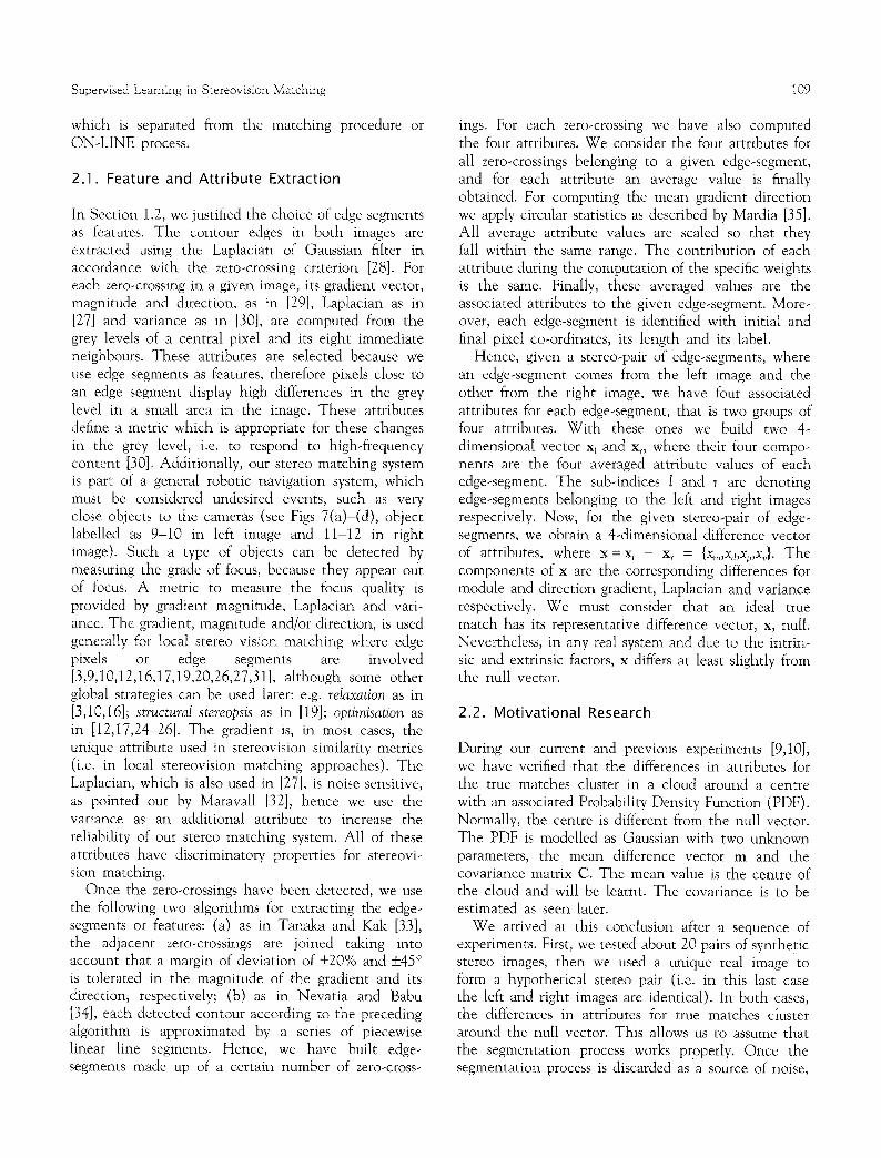
2.1. Feature and Attribute Extraction

In Section 1.2, we justified the choice of edge segments as features. The contour edges in both images are extracted using the Laplacian of Gaussian filter in accordance with the zero-crossing criterion [28]. For each zero-crossing in a given image, its gradient vector, magnitude and direction, as in [29], Laplacian as in [27] and variance as in [30], are computed from the grey levels of a central pixel and its eight immediate neighbours. These attributes are selected because we use edge segments as features, therefore pixels close to an edge segment display high differences in the grey level in a small area in the image. These attributes define a metric which is appropriate for these changes in the grey level, i.e. to respond to high-frequency content [30]. Additionally, our stereo matching system is part of a general robotic navigation system, which must be considered undesired events, such as very close objects to the cameras (see Figs 7(a)-(d), object labelled as 9-10 in left image and 11-12 in right image). Such a type of objects can be detected by measuring the grade of focus, because they appear out of focus. A metric to measure the focus quality is provided by gradient magnitude, Laplacian and variance. The gradient, magnitude and/or direction, is used generalIy for local stereo vision matching where edge pixels or edge segments are involved [3,9,10,12,16,17,19,20,26,27,31], although some other global strategies can be used later: e.g. relaxation as in [3,10,16]; structural stereopsis as in [19]; optimisation as in [12,17,24-26]. The gradient is, in most cases, the unique attribute used in stereovision similarity metrics (i.e. in local stereovision matching approaches). The Laplacian, which is also used in [27], is noise sensitive, as pointed out by Maravall [32], hence we use the variance as an additional attribute to increase the reliability of our stereo matching system. All of these attributes have discriminatory properties for stereovision matching.

Once the zero-crossings have been detected, we use the following two algorithms for extracting the edge- segments or features: (a) as in Tanaka and Kak [33], the adjacent zero-crossings are joined taking into account that a margin of deviation of _+20% and _+45 ~ is tolerated in the magnitude of the gradient and its direction, respectively; (b) as in Nevatia and Babu [34], each detected contour according to the preceding algorithm is approximated by a series of piecewise linear line segments. Hence, we have built edge- segments made up of a certain number of zero-cross-

ings. For each zero-crossing we have also computed the four attributes. We consider the four attributes for all zero-crossings belonging to a given edge-segment, and for each attribute an average value is finally obtained. For computing the mean gradient direction we apply circular statistics as described by Mardia [35]. All average attribute values are scaled so that they fall within the same range. The contribution of each attribute during the computation of the specific weights is the same. Finally, these averaged values are the associated attributes to the given edge-segment. More- over, each edge-segment is identified with initial and final pixel co-ordinates, its length and its label.

Hence, given a stereo-pair of edge-segments, where an edge-segment comes from the left image and the other from the right image, we have four associated attributes for each edge-segment, that is two groups of four attributes. With these ones we build two 4- dimensional vector xl and x~, where their four components are the four averaged attribute values of each edge-segment. The sub-indices l and r are denoting edge-segments belonging to the left and right images respectively. Now, for the given stereo-pair of edge- segments, we obtain a 4-dimensional difference vector of attributes, where x =xt - Xr = {X,,I,Xd,Xp,Xv}. The components of x are the corresponding differences for module and direction gradient, Laplacian and variance respectively. We must consider that an ideal true match has its representative difference vector, x, null. Nevertheless, in any real system and due to the intrinsic and extrinsic factors, x differs at least slightly from the null vector.

2.2. Motivational Research

During our current and previous experiments [9,10], we have verified that the differences in attributes for the true matches cluster in a cloud around a centre with an associated Probability Density Function (PDF). Normally, the centre is different from the null vector. The PDF is modelled as Gaussian with two unknown parameters, the mean difference vector m and the covariance matrix C. The mean value is the centre of the cloud and will be learnt. The covariance is to be estimated as seen later.

We arrived at this conclusion after a sequence of experiments. First, we tested about 20 pairs of synthetic stereo images, then we used a unique real image to form a hypothetical stereo pair (i.e. in this last case the left and right images are identical). In both cases, the differences in attributes for true matches cluster around the null vector. This allows us to assume that the segmentation process works properly. Once the segmentation process is discarded as a source of noise,


we design new experiments with real stereo images captured with two cameras, C1 and C2. We placed our stereovision system in 43 different positions in the working environment under different illumination conditions. These images are different from the ones used in this paper for testing the LVQ approach. At each position we capture a pair of stereo images, one with C, placed to the left of C2 (configuration A) and another one with C1 placed to. the right of Cz (configuration B). Therefore, for each configuration we have 43 stereo images available, from where we obtain 1025 difference vectors of attributes for true matches (xa, and xBi where i = 1..1025). The true matches are selected under the human expert criterion. For each coraponent, module and direction gradient, Laplacian and variance, of Xgi and xBi, we perform the corresponding histograms. We observe that the histograms in both, A and B, configurations have a form that could be considered a Gauss's bell. We obtain two mean values for each component, one for each configuration, and we observe that these two mean values have a similar magnitude (different from the null value) but opposite signs (e.g. the estimated mean value for the gradient direction with the configuration A is 0.181 and with configuration B is -0.184).

We conclude that (a) the Gauss's bell form is due to the extrinsic factors, (b) the magnitude of the mean values are due to the intrinsic factors, and (c) the different sign comes from the two different configurations, A and B. These conclusions allow us to assume that this is applicable to the 4-dimensional space assuming a multivariate PDF, and justify the assump- tions made about the Gaussian form of the PDF and

the clustering of the differences in attributes for true matches around a centre.

2.3. Training Process: Supervised Learning Applied to Stereovision Matching

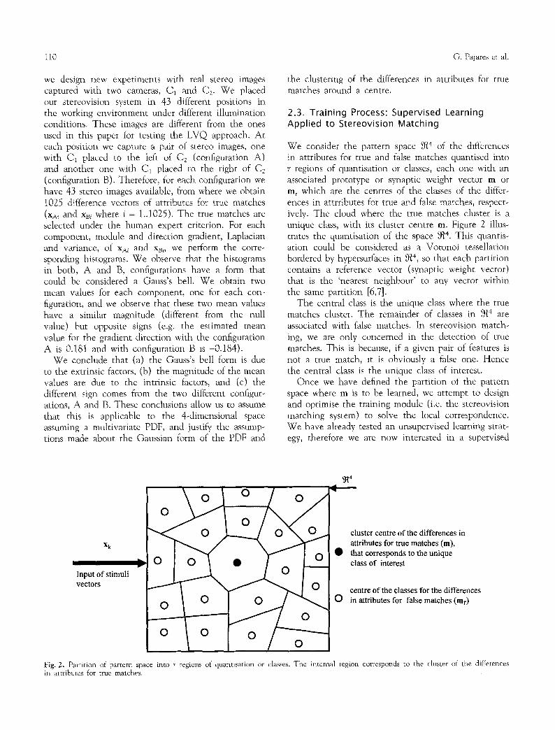
We consider the pattern space ~4 of the differences in attributes for true and false matches quantised into r regions of quantisation or classes, each one with an associated prototype or synaptic weight vector m or mr which are the centres of the classes of the differences in attrributes for true and false matches, respectively. The cloud where the true matches cluster is a unique class, with its cluster centre m. Figure 2 illus- trates the quantisation of the space 9t 4. This quantisation could be considered as a Voronoi tessellation bordered by hypersurfaces in 914, so that each partition contains a reference vector (synaptic weight vector) that is the 'nearest neighbour' to any vector within the same partition [6,7].

The central class is the unique class where the true matches cluster. The remainder of classes in {)~4 a r e associated with false matches. In stereovision matching, we are only concerned in the detection of true matches. This is because, if a given pair of features is not a true match, it is obviously a false one. Hence the central class is the unique class of interest.

Once we have defined the partition of the pattern space where m is to be learned, we attempt to design and optimise the training module (i.e. the stereovision matching system) to solve the local correspondence. We have already tested an unsupervised learning strategy, therefore we are now interested in a supervised

Xk

Input of stimuli vectors

~4

o l A O O

cluster centre of the differences in attributes for true matches (m),

�9 that corresponds to the unique class of interest

centre of the classes for the differences ~ O in attributes for false matches (mr)

Fig. 2. Partition of pattern space into r regions of quanttsation or classes. The internal region corresponds to the cluster of the differences in attributes for true matches.


learning approach, because the learning with a teacher seems to be more effective. We choose the supervised LVQ method because it is appropriate to deal with the partition of the previously defined pattern space, which typifies the stereovision matching problem. Therefore, according to the above and following Pat- terson [7], the LVQ should be summarised as follows:

(a) Select a set of n stimuli vectors X = {xl ,xi , . . . ,x~}.

(b) Initialise m, and n~ to small random numbers.

(c) For each input pattern x~, where k = 1,2,...n, select the corresponding known output target class, t. Let Cl(Xk) denote the class of xk computed by the system. C/(xk) is found by using a minimum distance criterion, i.e. mini d(mj,xk), where the sub-index j denotes the number of classes and mj is the corresponding class centre vector, d(mj,xk) is a distance between m; and xk, typically it is the Euclidean distance.

(d) When the class is correct (C/(xk) = t) the centre vector of the corresponding class is shifted towards the input pattern vector. When an incorrect class is selected by the system (Cl(xk) # t), the centre vector is shifted away from the input pattern vector.

From the LVQ we derive our supervised learning approach to be applied to our stereovision matching problem as follows:

(a) We select a set of n stimuli vectors X = {x~,xz,...,x,l}, which are potential true matches according to the initial correspondence carried out by the image analysis module (section 2). Therefore, the stimuli vectors in X represent differences in attributes of true matches.

(b) Taking into account that we are only concerned with the detection of true matches, we have decided that the learning in our model is performed only by the central class. So we initialise m to the ideal cluster centre (m = 0).

(c) For each input pattern xk in X, where k ranges from 1 to n, the central class is the target one where the input pattern should be classified. To decide if the input pattern really belongs to the target class, we use a metric based on the squared Mahalanobis distance between m and xk, dv(m,xk), and then if dM(m,xk) --< R we assume that x> in fact, belongs to the central class (i.e. to the class of true matches). The squared Mahal- anobis distance is given by dM(xk,m) = (xk -- m) ~ C<(xk - m) [32,36]. The super index t denotes transpose. The covariance matrix C used in the computation of dM(x>m) measures the dispersion of the stimuli vectors in the cluster, and it is the

(dl

one obtained during the last OFF-LINE process, since the one corresponding to the current OFF- LINE process is not available yet. Initially, it is set to the identity matrix.

When the input pattern is classified by the system as belonging to the central class (C/(xk) = t), according to the squared Mahalanobis distance criterion, the centre vector of this class m is shifted towards the input vector x> Otherwise, the input pattern vector does not belong to the target class (Cl(xk) # t), the centre vector of the central (target) class is shifted away from the input pattern vector. This process is summarised in the following equation:

m ( k + 1) re(k) + ~1 [xk - m ( k ) l ,

m ( k ) - ~1 [xk - re(k)],

if dM(x>m(k) ) <- T

otherwise

(,)

where m(k) is the corresponding value for the cluster centre vector before the stimulus xk is processed, and the vector re(k+1) is the corresponding cluster centre vector after xk is processed, r I is the learning rate or learning coefficient that controls the amount of change in m; T is a decision threshold.

2.3.1. Improving the Learning Rate. Following Wu [8], a practical choice for the learning rate r~ is 0.1 < rl < 1.0. Nevertheless, the choice of such coefficient is a hard task, because we are never sure which is the best value to be selected. At this point, and after an exhaustive analysis, we have introduced an improvement and a better performance in our stereovision matching system. The learning rate is considered variable and depends on: (a) the training sample (pair of features) under processing through rio, and (b) the amount of training performed through rlk. So the learning rate can be computed as ~/= rlor/k.

Computation of ~/o. The system is matching edge segments which come from a pair of cameras previously aligned. So, we can assume that if an edge-segment in a given image is slid following a horizontal direction or epipolar line, it must intersect its corresponding couple in the other image. Hence, we define "q as an overlap rate, which is computed as the rate of coincidence from the corresponding lengths (see Section 2 and Fig. 1), and is given as follows:

2lc rio - lz + lr (2 )

where /~ is the common overlap length, and lz, l~ are


the corresponding lengths for left and r ight edge- segments under matching. All lengths a~g'measured in pixels. Nevertheless, r/ is bounded in the interval (0.1, 1) as suggested by Wu [8].

This improvement is justified and based on the following two reflections:

1. The edge segments to be matched are extracted after a tough process (Section 2.1), where broken edge segments are reconstructed, i.e. the edge segments should appear with their corresponding full lengths.

2. This variable learning rate could be considered as an a priori matching probability and avoids us to fix a constant value for the learning rate. We are never sure which is the best constant value.

Computation of r/k. The factor r/k defines a decreasing sequence of positive numbers on the interval (0,1)]. This kind of learning rate is commonly used in Self- Organizing Feature Maps [5,37-39], where numerous simulations have shown that the best results are obtained if it is selected fairly wide in the beginning and then permitted to shrink with iteration k, and fulfils ~k ---+ 0, k ~ oo. We follow this criterion, and define r;k as

1 "qk - a + k (3)

where a is an integer constant, that after experimentation in our work it has been fixed to 60; ~/k decreases as the number of samples increases according to the following law: the learning rate decreases as learning pro- gresses.

This definition of the learning rate introduces an important improvement with regard to previous research works involving unsupervised learning UL [9,10] and SOM [11].

In UL, the learning rate is computed as follows:

p(xk) c < - k (4)

i=1

where p(xi) is the matching probability of the pattern stimulus x~ associated to the central class, and it is computed as a decreasing exponential function of the Mahalanobis distance, defined by the Gaussian PDF. This central class is where the differences in attribute values for true matches cluster, as in this paper. The denominator in Eq. (4) grows with the number of iterations k. In our experiments, for values of k under 100, the number of training patterns is not still significant, and the values of the learning rate c~k are

high. This leads to undesired large variability in m at this initial training phase, which affects to the final results. We avoid this by introducing the constant value a in ~k; nevertheless, this is not a limitation for other applications, because this value could be permanently set to 1.

In SOM ~ = h(d)r/k, where r/k is computed as in Eq. (3) and h(d) is a neighbourhood function involving the squared Mahalanobis distance

1 h(d) - (5)

l+dM(xk,mk)

In this paper, we avoid the redundant use of the squared Mahalanobis distance dv(xk,mk) by using Eq. (1) instead of Eq. (5).

Finally, as stated before, we must estimate the covariance matrix C to get the second parameter of the PDF describing the cluster of interest. This process is carried out following the same criterion that the one used for updating m through Eq. (1), where as before, the same set of n stimuli vectors is supplied (i.e. processed):

c(k + 1) = (6)

C(k) + r/[(xk-m(k))~(xk m(k)) -C(k)] ifd~(xk,m(k)) <-T C(k) - r~[(xk - m(k))~(xk - m(k))-C(k)] otherwise

It is important to point out that re(k) is the value computed through Eq. (1) during the current OFF- LINE process; ~ is, as before, computed by Eqs (2) and (3); C(k) and C(k + 1) are the covariance matrices before and after the stimulus xk is processed, respectively. Finally, t denotes transpose.

The covariance matrix gives us information about the cross-correlation between attributes [32], which provides a method to verify the possible use of redundant attributes that could be avoided and, as a result, the computational cost reduced.

2.3.2. Computation of the Importance of the Attri- butes for Matching. To compare the importance of our attributes with those of Lew et al ( [27], we obtain the specific weight wsj of the attributes for matching after each OFF-LINE training process.

We start taking into account that initially, that is before the first OFF-LINE process, the cluster centre corresponding to the central class of true matches m is set to the null vector. This is derived under the assumption that without knowledge of the behaviour of the system, it is the best. Then, as the training increases, during subsequent OFF-LINE processes m is shifted away from the null vector when the match is classified as true by the system. This fact allows us to


formulate the following hypothesis: a maximum deviation from 0 for each component in m corresponds to a minimum specific weight for the associated attribute, and vice versa. Based on this assumption, and given the last coraputed cluster centre vector m, we obtain each one of the four components of the specific weight vector w~ as follows:

Im, I (7) WsJ-- 4

Y lm l k=I

where mj (mk) in the right-hand side of the above equation are the components of the learned cluster centre vector, obtained according to Eq. (1). As mentioned before, indices j and k take values 1, 2, 3 and 4 associated with magnitude and direction gradient, Laplacian and variance attributes, respectively. Each w~j ranges from 0 to 1, and the sum of the four w~j is 1.

2.4. The Current Stereo Matching Process

This is an ON-LINE process in which a pair of new stereo images are to be matched. The image analysis system extracts pairs of features and supplies their corresponding four-dimensional difference vectors of the attributes x, to the stereo matching system. For each x received, the system computes the squared Mahalanobis distance dv(x,m), where the involved cluster centre m and the covariance matrix (2 are the ones updated during the last OFF-LINE training process according to Eqs (1) and (6). The incoming pair of features is classified as a true match if dM(x,m) is less than T, otherwise it is a false match. T is the decision threshold introduced in Eq. (1).

3. COMPARATIVE ANALYSIS AND PERFORMANCE EVALUATION

To assess the validity and performance of our method, we design a test strategy with four goals:

1. To show the validity of the learning process, i.e. to show how results are improved as the learning process grows.

2. To show the effectiveness of our method as compared to classical local stereo matching techniques KA [16] and MN [3], and other more recent learning local methods UL [9,t0] and SOM [11] (Section 1.4).

3. To compare the better performance of HOP [12] when the squared Mahalanobis distance, as in this

paper, is used instead of the squared Euclidean distance.

4. To compare our most significant attributes with the set of attributes used in LHW [27].

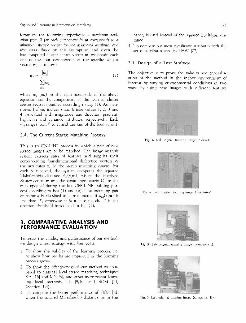
3.1. Design of a Test Strategy

The objective is to prove the validity and generalis- ation of the method in the indoor environment of interest by varying environmental conditions in two ways: by using new images with different features

Fig. 3. Left original training image (blocks).

Fig. 4. Left original training image (furnitures).

v <~ 4,#: ,

Fig. 5. Left original training image (computers I).

Fig. 6. Left original training image (computers II).


(different objects), and by changing the illumination. With this aim in mind, and the four goals pointed out before, 12 pairs of stereo images captured with natural illumination are used as initial samples. Figures 3, 4, 5 and 6 show four representative left images. Furthermore, three sets of stereo-images, which are different from each other and from the initial samples, are used and will constitute the inputs for the test: SP1, SP2 and SP3 with 10, 10 and 15 stereo-images. Therefore, the number of stereo images is 47, the total number of pairs of edge segments processed is 2132 (i.e. the number of potential true matches supplied by the image analysis module). This last number is detached in 1187 stereo pairs classified as true matches by the current stereo matching module (i.e. dv(xk,m) is less than R for such pairs), which are used as training samples for the training module to shift the cluster centre m towards the corresponding input pattern vector x> The remainder stereo pairs are classified

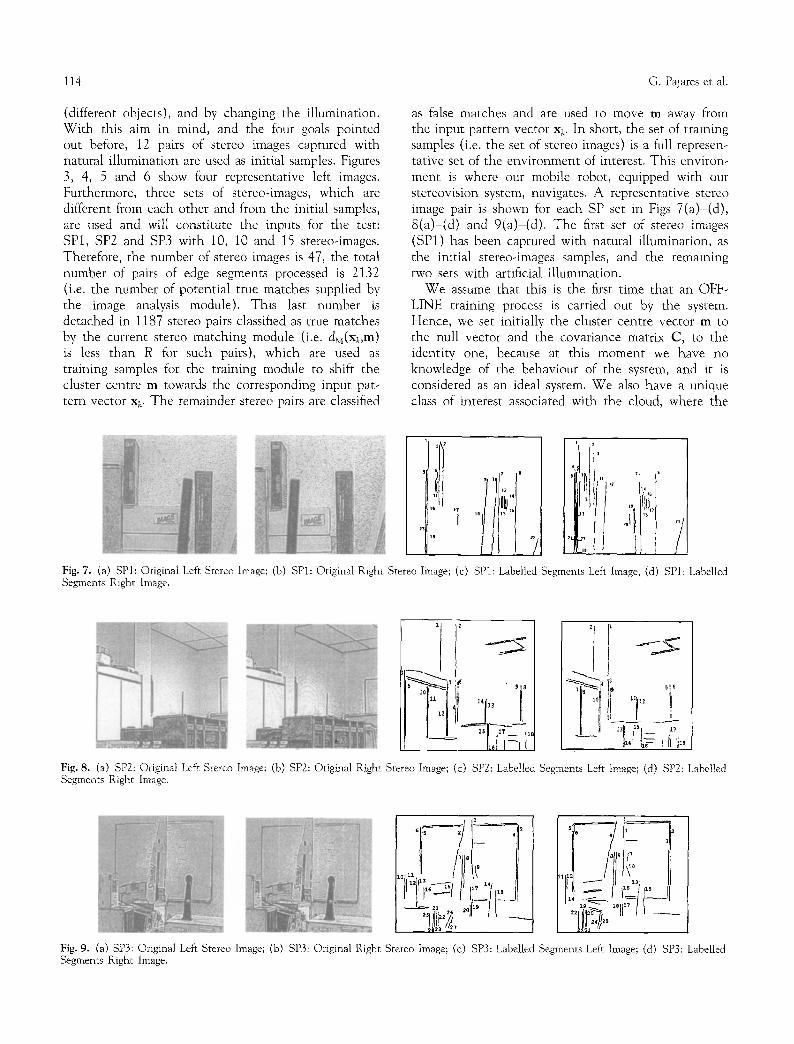
as false matches and are used to move m away from the input pattern vector xk. In short, the set of training samples (i.e. the set of stereo images) is a full representative set of the environment of interest. This environment is where our mobile robot, equipped with our stereovision system, navigates, a representative stereo image pair is shown for each SP set in Figs 7(a)-(d), 8(a)-(d) and 9(a)-(d). The first set of stereo images (SP1) has been captured with natural illumination, as the initial stereo-images samples, and the remaining two sets with artificial illumination.

We assume that this is the first time that an OFF- LINE training process is carried out by the system. Hence, we set initially the cluster centre vector m to the null vector and the covariance matrix C, to the identity one, because at this moment we have no knowledge of the behaviour of the system, and it is considered as an ideal system. We also have a unique class of interest associated with the cloud, where the

s 1 �9 a

II 12 14 i ~ t15

" [ 7

tl/ 1~ 7

16

~ai s 17

/ Fig. 7. (a) SPI: Original Left Stereo Image; (b) SPI: Original Right Stereo Image; (c) SPI: Labelled Segments Left Image; (d) SPI: Labelled Segments Right Image.

Fig. 8. (a) SP2: Original Left Stereo Image; (b) SP2: Original Right Segments Right image.

I f'~I ~ , , ~ I

Stereo Image; (c) SP2: Labelled Segments Left Image; (d) SP2: Labelled

I /l

2~ 22 26 ,l!l,a,

~ 3 S6 4 1

~ /~o

Fig. 9. (a) SP3: Original Left Stereo Image; (b) SP3: Original Right Stereo hnage; (c) SP3: Labelled Segments Left Image; (d) SP3: Labelled Segments Right Image.


differences in attributes for the true matches cluster around a centre m. With this approach the size of the cloud is constant, but the cloud position varies as the cluster centre vector m changes after each OFF-LINE training process, i.e. during the following four test steps.

The test process tries to show the learning effectiveness and involves the four steps in which the cluster centre and specific weight vectors are updated:

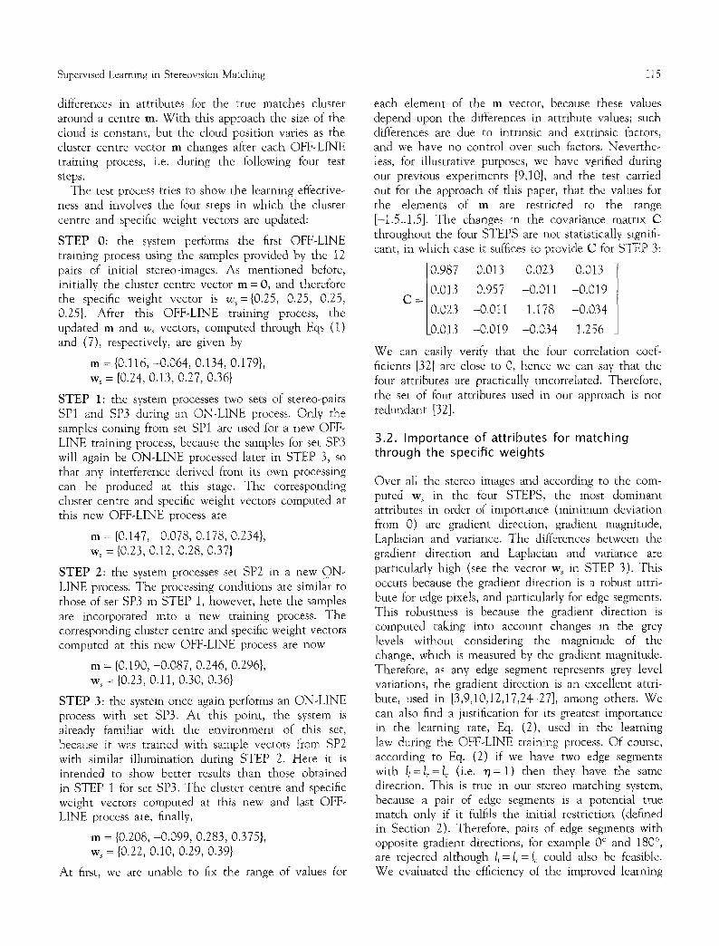
STEP O: the system performs the first OFF-LINE training process using the samples provided by the 12 pairs of initial stereo-images. As mentioned before, initially the cluster centre vector m = O, and therefore the specific weight vector is %={0.25, 0.25, 0.25, 0.25}. After this OFF-LINE training process, the updated m and w~ vectors, computed through Eqs (1) and (7), respectively, are given by

m = {0.116, -0.064, 0.134, 0.179}, ws = {0.24, 0.13, 0.27, 0.36}

STEP 1: the system processes two sets of stereo-pairs SP1 and SP3 during an ON-LINE process. Only the samples coming from set SP1 are used for a new OFF- LINE training process, because the samples for set SP3 will again be ON-LINE processed later in STEP 3, so that any interference derived from its own processing can be produced at this stage. The corresponding cluster centre and specific weight vectors computed at this new OFF-LINE process are

m = {0.147, -0.078, 0.178, 0.234}, ws = {0.23, 0.12, 0.28, 0.37}

STEP 2: the system processes set SP2 in a new ON- LINE process. The processing conditions are similar to those of set SP3 in STEP 1, however, here the samples are incorporated into a new training process. The corresponding cluster centre and specific weight vectors computed at this new OFF-LINE process are now

m = {0.190, -0.087, 0.246, 0.296}, ws = {0.23, 0.11, 0.30, 0.36}

STEP 3: the system once again performs an ON-LINE process with set SP3. At this point, the system is already familiar with the environment of this set, because it was trained with sample vectors from SP2 with similar illumination during STEP 2. Here it is intended to show better results than those obtained in STEP 1 for set SP3. The cluster centre and specific weight vectors computed at this new and last OFF- LINE process are, finally,

m = {0.208, -0.099, 0.283, 0.375}, ws = {0.22, 0.10, 0.29, 0.39}

At first, we are unable to fix the range of values for

each element of the m vector, because these values depend upon the differences in attribute values; such differences are due to intrinsic and extrinsic factors, and we have no control over such factors. Neverthe- less, for illustrative purposes, we have v.erified during our previous experiments [9,10], and the test carried out for the approach of this paper, that the values for the elements of m are restricted to the range [-1.5..1.5]. The changes in the covariance matrix C throughout the four STEPS are not statistically significant, in which case it suffices to provide C for STEP 3:

0.987 0.013 0.023 0.013

|0.013 0.957 -0.011 -0.019

C = ||0.023 -0.011 1.178 -0.034

L0.013 -0.019 -0.034 1.256

We can easily verify that the four correlation coef- ficients [32] are close to 0, hence we can say that the four attributes are practically uncorrelated. Therefore, the set of four attributes used in our approach is not redundant [321.

3.2. Importance of attributes for matching through the specific weights

Over all the stereo images and according to the computed w~ in the four STEPS, the most dominant attributes in order of importance (minimum deviation from 0) are gradient direction, gradient magnitude, Laplacian and variance. The differences between the gradient direction and Laplacian and variance are particularly high (see the vector ws in STEP 3). This occurs because the gradient direction is a robust attribute for edge pixels, and particularly for edge segments. This robustness is because the gradient direction is computed taking into account changes in the grey levels without considering the magnitude of the change, which is measured by the gradient magnitude. Therefore, as any edge segment represents grey level variations, the gradient direction is an excellent attribute, used in [3,9,10,12,17,24-27], among others. We can also find a justification for its greatest importance in the learning rate, Eq. (2), used in the learning law during the OFF-LINE training process. Of course, according to Eq. (2) if we have two edge segments with lt=l~=lc (i.e. rl= 1) then they have the same direction. This is true in our stereo matching system, because a pair of edge segments is a potential true match only if it fulfils the initial restriction (defined in Section 2). Therefore, pairs of edge segments with opposite gradient directions, for example 0 ~ and 180 ~ are rejected although lz= l~ = lo could also be feasible. We evaluated the efficiency of the improved learning


rate using a constant learning rate. On average, when we set "q to a fixed value in the range (0..1), the percentage of successes obtained in each step is reduced in a quantity about 10%, compared to the results obtained by using the learning rate computed through Eqs (2) and (3), as shown in Table 1.

The sharpness of focus for an edge is detected by gradient magnitude, Laplacian and variance. Nevertheless, we can point out that the gradient magnitude is the second most important attribute, although they all measure the same. This occurs because the gradient magnitude is obtained taking the largest difference in grey levels of two opposite pixels in the corresponding 8.neighbourhood of a central pixel, whereas the Lapla- clan and variance use the nine involved pixels in the same 8-neighbourhood around the central pixel. This means that using the Laplacian and variance more central pixels would appear to be similar in different edge segments in the same pair of stereo images, because the values for these central pixels are averaged in the 8-neighbourhood.

3.3. Comparative Analysis

To compare the effectiveness of our supervised approach, we select the similarity metric used in the local stereovision matching technique proposed by KA [16] and MN [3] and, for comparison purposes, we use the squared Euclidean distance, as detailed in Section 1.4.

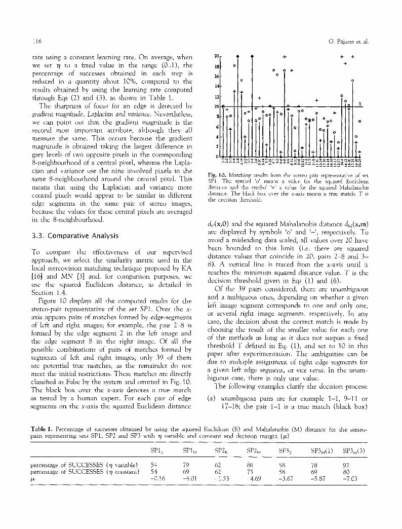
Figure 10 displays all the computed results for the stereo-pair representative of the set SP1. Over the x- axis appears pairs of matches formed by edge-segments of left and right images; for example, the pair 2-8 is formed by the edge segment 2 in the left image and the edge segment 8 in the right image. Of all the possible combinations of pairs of matches formed by segments of left and right images, only 39 of them are potential true matches, as the remainder do not meet the initial restrictions. These matches are directly classified as False by the system and omitted in Fig. 10. The black box over the x-axis denotes a true match as tested by a human expert. For each pair of edge segments on the x-axis the squared Euclidean distance

~o

16

14

12 I

lO I ,

81

6

4

ol -F

0 0 4- .~ §

ii

4-

§

O

,O O +

O~o] +oO

ill,li, 0 O 0 0

4-

O

o

4-

Fig. 10. Matching results from the stereo pair representative of set SP1. The symbol %' means a value for the squared Euclidean distance and the symbol '+' a value for the squared Mahalanobis distance. The black box over the x-axis means a true match. T is the decision threshold.

dE(x,O) and the squared Mahalanobis distance dv(x,m) are displayed by symbols 'o' and '+', respectively. To avoid a misleading data scaled, all values over 20 have been bounded to this limit (i.e. there are squared distance values that coincide in 20, pairs 2-8 and 3- 8). A vertical line is traced from the x-axis until it reaches the minimum squared distance value. T is the decision threshold given in Eqs (1) and (6).

Of the 39 pairs considered, there are unambiguous and a ambiguous ones, depending on whether a given left image segment corresponds to one and only one, or several right image segments, respectively. In any case, the decision about the correct match is made by choosing the result of the smaller value for each one of the methods as long as it does not surpass a fixed threshold T defined in Eq. (1), and set to 10 in this paper after experimentation. The ambiguities can be due to multiple assignment of right edge segments for a given left edge segment, or vice versa. In the unambiguous case, there is only one value.

The following examples clarify the decision process:

(a) unambiguous pairs are for example 1-1, 9-11 or 17-18; the pair 1-1 is a true match (black box)

Table 1. Percentage of successes obtained by using the squared Euclidean (E) and Mahalanobis (M) distance for the stereo- pairs representing sets SP1, SP2 and SP3 with ~/ variable and constant and decision margin (/x)

SP1E SP1M SP2E SP2M SP3E SP3M(1) SP3M(3)

percentage of SUCCESSES (7 variable) 54 79 62 86 58 78 92 percentage of SUCCESSES ('q constant) 54 69 62 75 58 69 80 /x -0.16 -4.01 -1.53 -4.69 -3.67 -5.87 -7.03


classified as true for d~ and false with dM because T is surpassed (failure); the pair 9-11 is a true match classified as true for both de and dv (success), but dv is smaller than de, i.e. the best decision is taken with dM; the pair 17-18 is a false match classified as false for both de and dM (success), but dM is greater than de, i.e. as above the best decision is taken with dM.

(b) ambiguous pairs are 2-2, 2-3, 2-6, 2-8, 2-14; the pair 2-2 with de is classified as true and the method would fail, since the true match is 2-3. With dM is 2-3 classified as true (success); a set of ambiguous pairs is (15-15, 15-17); with both de and dv the pair 15-17 is classified as a true match (success), but dM is smaller than dE, and the best decision is taken with dM; in this example, in general, the best results (minimum/maximum squared distance values for true/false matches) are obtained with the squared Mahalanobis distance.

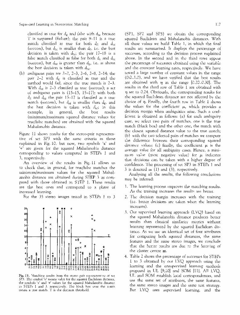
Figure 11 shows results for the stereo-pair representative of set SP3 with the same criteria as those explained in Fig. 10, but now, two symbols 'x' and '+' are given for the squared Mahalanobis distance corresponding to values computed in STEPs 1 and 3, respectively.

An overview of the results in Fig. 11 allows us to check that, in general, for true/false matches the minimum/maximum values for the squared Mahal- anobis distance are obtained during STEP 3 as compared with those obtained in STEP 1. These results are the best ones and correspond to a phase of increased learning.

For the 35 stereo images tested in STEPs 1 to 3

16

14

o

8

6 I

2a2~g~

m ~ o

x § X o

§

' X

T

o~ 0 §

Illl ~ 4 g d d a a . . . . . . . . . ~ ~ a ~

Fig. 11. Matching results from the stereo pair representative of set SP3. The symbol 'o' means value for the squared Euclidean distance, the symbols 'x' and '+' values for the squared Mahalanobis distance in STEPs 1 and 3, respectively. The black box over the x-axis means a true match. T is the decision threshold.

(SP1, SP2 and SP3) we obtain the corresponding squared Euclidean and Mahalanobis distances. With all these values we build Table 1, in which the final results are summarised. It displays the percentage of successes, according to the decision process explained above. In the second and in the third rows appear the percentage of successes obtained using the variable and the constant learning rates, respectively. We have tested a large number of constant values in the range (0.0..1.0), and we have verified that the best results are obtained with ~ in the range [0.20..0.30]. The results in the third row of Table 1 are obtained with rl set to 0.24. Obviously, the corresponding results for the squared Euclidean distance are not affected by the choice of r/. Finally, the fourth row in Table 1 shows the values for the coefficient /z, which provides a decision margin when ambiguities arise. Such a coefficient is obtained as follows: (a) for each ambiguity case, we select two pairs of matches, one is the true match (black box) and the other one, the match with the closest squared distance value to the true match; (b) with the two selected pairs of matches we compute the difference between their corresponding squared distance values; (c) finally, the coefficient > is the average value for all ambiguity cases. Hence, a minimum value (most negative value) for /z indicates that decisions can be taken with a higher degree of confidence. The processing of set SP3 in STEPs 1 and 3 is denoted as (1) and (3), respectively.

Analysing all the results, the following conclusions may be inferred:

1. The learning process improves the matching results. As the training increases the results are better.

2. The decision margin increases with the training (i.e. better decisions are taken when the learning increases).

3. Our supervised learning approach (LVQ) based on the squared Mahalanobis distance produces better results than classical similarity metrics without learning represented by the squared Euclidean distance. As we use an identical set of four attributes for computing both squared distances, the same features and the same stereo images, we conclude that the better results are due to the learning of the cluster centre m.

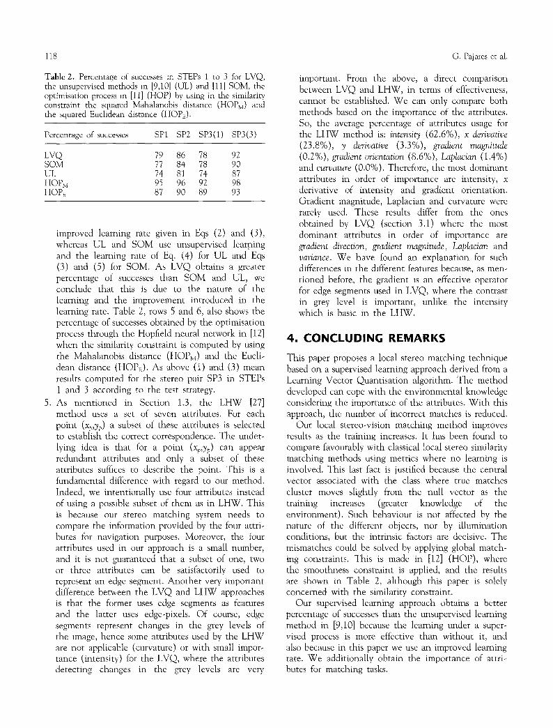
4. Table 2 shows the percentage of successes for STEPs 1 to 3 obtained by our LVQ approach using the learning and the unsupervised learning methods proposed in UL [9,10] and SOM [11]. All LVQ, UL and SOM establish local correspondences, and use the same set of attributes, the same features, the same stereo images and the same test strategy. But LVQ uses supervised learning, and the


Table 2. Percentage of successes in STEPs 1 to 3 for LVQ, the unsupervised methods in [9,10] (UL) and [11] SOM, the optimisation process in [11] (HOP) by using in the similarity constraint the squared Mahalanobis distance (HOPM) and the squared Euclidean distance (HOPE).

Percentage of successes SP1 SP2 SP3(1) SP3(3)

LVQ 79 86 78 92 SOM 77 84 78 90 UL 74 81 74 87 HOPM 95 96 92 98 HOPE 87 90 89 93

improved learning rate given in Eqs (2) and (3), whereas UL and SOM use unsupervised learning and the learning rate of Eq. (4) for UL and Eqs (3) and (5) for SOM. As LVQ obtains a greater percentage of successes than SOM and UL, we conclude that this is due to the nature of the learning and the improvement introduced in the learning rate. Table 2, rows 5 and 6, also shows the percentage of successes obtained by the optimisation process through the Hopfield neural network in [12] when the similarity constraint is computed by using the Mahalanobis distance (HOPM) and the Eucli- dean distance (HOPE). As above (1) and (3) mean results computed for the stereo pair SP3 in STEPs 1 and 3 according to the test strategy.

5. As mentioned in Section 1.3, the LHW [27] method uses a set of seven attributes. For each point (xp,yp) a subset of these attributes is selected to establish the correct correspondence. The under- lying idea is that for a point (xp,yp) can appear redundant attributes and only a subset of these attributes suffices to describe the point. This is a fundamental difference with regard to our method. Indeed, we intentionally use four attributes instead of using a possible subset of them as in LHW. This is because our stereo matching system needs to compare the information provided by the four attributes for navigation purposes. Moreover, the four attributes used in our approach is a small number, and it is not guaranteed that a subset of one, two or three attributes can be satisfactorily used to represent an edge segment. Another very important difference between the LVQ and LHW approaches is that the former uses edge segments as features and the latter uses edge-pixels. Of course, edge segments represent changes in the grey levels of the image, hence some attributes used by the LHW are not applicable (curvature) or with small importance (intensity) for the LVQ, where the attributes detecting changes in the grey levels are very

important. From the above, a direct comparison between LVQ and LHW, in terms of effectiveness, cannot be established. We can only compare both methods based on the importance of the attributes. So, the average percentage of attributes usage for the LHW method is: intensity (62.6%), x derivative (23.8%), y derivative (3.3%), gradient magnitude (0.2%), gradient orientation (8.6%), Laplacian (1.4%) and curvature (0.0%). Therefore, the most dominant attributes in order of importance are intensity, x derivative of intensity and gradient orientation. Gradient magnitude, Laplacian and curvature were rarely used. These results differ from the ones obtained by LVQ (section 3.1) where the most dominant attributes in order of importance are gradient direction, gradient magnitude, Laplacian and variance. We have found an explanation for such differences in the different features because, as mentioned before, the gradient is an effective operator for edge segments used in LVQ, where the contrast in grey level is important, unlike the intensity which is basic in the LHW.

4. CONCLUDING REMARKS

This paper proposes a local stereo matching technique based on a supervised learning approach derived from a Learning Vector Quantisation algorithm. The method developed can cope with the environmental knowledge considering the importance of the attributes. With this approach, the number of incorrect matches is reduced.

Our local stereo-vision matching method improves results as the training increases. It has been found to compare favourably with classical local stereo similarity matching methods using metrics where no learning is involved. This last fact is justified because the central vector associated with the class where true matches cluster moves slightly from the null vector as the training increases (greater knowledge of the environment). Such behaviour is not affected by the nature of the different objects, nor by illumination conditions, but the intrinsic factors are decisive. The mismatches could be solved by applying global matching constraints. This is made in [12] (HOP), where the smoothness constraint is applied, and the results are shown in Table 2, although this paper is solely concerned with the similarity constraint.

Our supervised learning approach obtains a better percentage of successes than the unsupervised learning method in [9,10] because the learning under a supervised process is more effective than without it, and also because in this paper we use an improved learning rate. We additionally obtain the importance of attributes for matching tasks.

Supervised Learning in Stereovision Matching

T h e stereo ma tch ing system is used for nav iga t ion purposes, and it is assembled over a mobi le robot. This nav iga t ion task is carr ied out in an indoor env i ron- ment . Hence , 47 stereo images were chosen from this env i ronmen t . This number of stereo images, t aken under different i l l umina t ion condi t ions (sect ion 3.1), is representa t ive of the e n v i r o n m e n t of interest , in which edge segments are prevalent , and it suffices for the nav iga t ion objec t ive in such an indoor envi ron- ment . A l t h o u g h we t reat the special case of edge segments as ma tch ing features, we argue tha t the me thod in t roduced in this paper can be easily general - ised to most features (i.e. pixels, curves, regions) where a set of a t t r ibutes should be defined. A t this moment , o the r tyes of env i ronmen t s are outside our area of interest , such as ou tdoor scenes or aerial images, where edge segments are probably no t appropr ia te features, and therefore different features and at t r ibutes should

be suitable.

Acknowledgements

Part of the work has been performed under project C I C Y T TAP94-0832-C02-O1. T h e authors wish to acknowledge Dr S. Dormido, Head of Depa r tme n t of Informfit ica y Automfi t ica , C C Ffsicas, U N E D , Madrid , for his support and encouragement .

R e f e r e n c e s

1. Lee SH, Leou JJ. A dynamic programming approach to line segment matching in stereo vision. Pattern Recognition 1994; 27:961-986

2. Mart D, Poggio T. A computational theory of human stereovision. Proc Roy Soc Lond B 1979; 207:301-328

3. Medioni G, Nevatia R. Segment based stereo matching. Com- puter Vision, Graphics and hnage Processing 1985; 31:2-18

4. Pollard SB, Mayhew JEW, Frisby JP. PMF: A stereo correspondence algorithm using a disparity gradient limit. Perception 1981; 14:449470

5. Kohonen T. Self-Organization and Associative Memory, Springer-Verlag, New York, 1989

6. Kohonen T. Self-Organizing Maps, Springer-Verlag, Berlin, 1995 7. Patterson DW. Artificial Neural Networks, Prentice-Hall, Singa-

pore, 1996 8. Wu JK. Neural Networks and Simulation Methods, Marcel

Dekker, New York, 1994 9. Cruz JM, Pajares G, Aranda J. A neural network approach to the

stereovision correspondence problem by unsupervised learning. Neural Networks 1995; 8(5): 805-813

10. Pajares G. Estrategia de Solucion al Problema de la Correspond- encia en Vision Estereosc6pica por la Jerarqufa Metodoldgica y [a lntegracidn de Criterios. PhD thesis, Dpto. Informfitica y Automfitica, Facultad Ciencias UNED: Madrid, 1995

11. Pajares G, Cruz JM, Aranda J. Stereo matching based on the self-organizing feature mapping algorithm. Pattern Recognition Letters 1998 (accepted)

12. Pajares G, Cruz JM, Aranda J. Relaxation by Hopfield network

119

in stereo image matching. Pattern Recognition 1998; 31(5): 561-574

13. Dhond AR, Aggarwal JK. Structure from stereo - a review. IEEE Trans Syst Man Cybern 1989; I9:1489-1510

14. Ozanian T. Approaches for stereo matching - a review. Mode- ling Identification Control 1995; 16(2): 65-94

15. Fua P. A parallel algorithm that produces dense depth maps and preserves image features. Machine Vision and Applic 1993; 6:35M9

16. Kim YC, Aggarwal JK. Positioning three-dimensional objects using stereo images. IEEE J Robotics and Automation 1987; 3(4): 361-373

17. Mousavi MS, Schalkoff RJ. ANN Implementation of stereo vision using a multi-layer feedback architecture. IEEE Trans Sys Man Cybern 1994; 24(8): 1220-1238

18. Ayache N, Faverjon B. Efficient registration of stereo images by matching graph descriptions of edge segments. Int J Computer Vision 1987; 1:107-131

19. Ayache N. Artificial Vision for Mobile Robots: Stereo Vision and Multisensory Perception, MIT Press, Cambridge, MA, 1991

20. Kim DH, Choi WY, Park RH. Stereo matching technique based on the theory of possibility. Patt Recognition Letters 1994; 13: 735-744

21. Hoff W, Ahuja N. Surface from stereo: integrating feature matching, disparity estimation, and contour detection. IEEE Trans Patt Anal Machine Intell 1989; 11:121-136

22. Wuescher DM, Boyer KL. Robust contour decomposition using a constraint curvature criterion. IEEE Trans Patt Anal Machine lntell 1991; 13(1): 41-51

23. Breuel TM. Finding lines under bounded error. Pattern Recog- nition 1996; 29 (1): 167-178

24. Zhou Y, Chellapa R. Artificial Neural Networks for Computer Vision, Springer-Verlag, Berlin, 1992

25. Yu SS, Tsai WH. Relaxation by the Hopfield neural network. Pattern Recognition 1992; 25(2): 197-209

26. Ruichek Y, Postaire JG. A neural matching algorithm for 3- D reconstruction from stereo pairs of linear images. Pattern Recognition Letters 1996; 17:387-398

27. Lew MS, Huang TS, Wong K. Learning and feature selection in stereo matching. IEEE Trans Part Anal Machine Intell 1994; 16(9): 869-881

28. Huertas A, Medioni G. Detection of intensity changes with subpixel accuracy using Laplacian-Gaussian masks. IEEE Trans Patt Anal Machine Intell 1986; 8(5): 651-664

29. Leu JG, Yau HL. Detecting the dislocations in metal crystals from microscopic images. Pattern Recognition 1991; 24(1): 41-56

30. Krotkov EP. Active Computer Vision by Cooperative focus and Stereo, Springer-Verlag, Berlin, 1989

31. Kahn P, Kitchen L, Riseman EM. A fast line finder for vision- guided robot navigation. IEEE Trans Part Anal Machine Intell 1990; 12(11): 1098-1102

32. Maravall D. Reconocimiento de Formas y Visi6n Artificial, RA- MA, Madrid, 1993

33. Tanaka S, Kak AC. A rule-based approach to binocular stereopsis. In: Jain RC, Jain AK (eds) Analysis and Interpretation of Range Images, Springer-Verlag, 1990

34. Nevatia R, Babu KR. Linear feature extraction and description. Computer Vision, Graphics and linage Process 1980; 13: 257- 269

35. Mardia KV. Statistics of Directional Data, Academic Press, London, 1972

36. Duda RO, Hart PE. Pattern Classification and Scene Analysis. Wiley, New York, 1973

37. Kosko B. Neural Networks and Fuzzy Systems, Prentice-Hall, Englewood Cliffs, NJ, 1992


38. Martin-Smith P, Pelayo FJ, Diaz A, Ortega J, Prieto A. A learning algorithm to obtain self-organizing maps using fixed neighbourhood Kohonen networks. In: Mira J, Cabestany J, Prieto A (eds), New Trends in Neural Computation, Springer- Verlag, 1993, 297-304

39. Haykin S. Neural Networks: A Comprehensive Foundation, Macmillan. New York, 1994

G. Pajares received the BS and PhD degrees in physics from UNED (Distance University of Spain) (1987, 1995) discussing a thesis on the application of pattern recognition techniques to stereovision. Since 1990 he has worked at ENOSA in critical software development. He joined in the Complutense University in 1995 as an Associate Professor in Robotics. His current research interests include robotic vision systems and applications of automatic control to robotics.

Jesfis M. de la Cruz received an MSc degree in Physics and a PhD from the Complutense University in 1979 and 1984, respectively. From 1985 to 1990 he was with the Department of Automatic Control,

UNED (Distance University of Spain), and from October 1990 to 1992 with the Depamnent of Electronics, University of Santander. In October 1992 he joined the Department of Computer Science and Automatic Control of the Complutense University, where he is a professor. His current research interests include robotic vision systems, multisensor data fusion and applications of automatic control to robotics and flight control.

Jose A. Lopez,Orozco received an MSc degree in Physics from the Complutense University in 1991. From 1992 to 1994 he had a Fellow- ship to work on Inertial Navigation Systems. Since 1995 he has been an assistant researcher in robotics at the Department of Computers Architecture and Automatic Control, where he is working for his PhD. His current research interests are robotics vision systems and multisensor data fusion.

Correspondence and offprint requests to: G. Pajares, Dpto. Arquitectura de Computadores y Automfitica, Facultad de CC. Ffsicas, Universi- dad Complutense, 28040 Madrid, Spain. E-mail: parajes@euc- max.sim.ucm.es

Improving stereovision matching through supervised learning

Documents

Transcript of Improving stereovision matching through supervised learning