Error Evaluation in a Stereovision-Based 3D Reconstruction System

Hindawi Publishing CorporationEURASIP Journal on Image and Video ProcessingVolume 2010, Article ID 539836, 12 pagesdoi:10.1155/2010/539836

Research Article

Error Evaluation in a Stereovision-Based3D Reconstruction System

Abdelkrim Belhaoua,1 Sophie Kohler,2 and Ernest Hirsch1

1 LSIIT (UMR CNRS-UdS 7005), Universite de Strasbourg, Bd Sebastien Brant, BP 10413, 67412 Illkirch Cedex, France2 MIPS (EA 2332), Universite Haute Alsace, 12, rue des freres Lumiere, 68093 Mulhouse Cedex, France

Correspondence should be addressed to Sophie Kohler, [email protected]

Received 1 December 2009; Revised 21 May 2010; Accepted 29 June 2010

Academic Editor: Pascal Frossard

Copyright © 2010 Abdelkrim Belhaoua et al. This is an open access article distributed under the Creative Commons AttributionLicense, which permits unrestricted use, distribution, and reproduction in any medium, provided the original work is properlycited.

The work presented in this paper deals with the performance analysis of the whole 3D reconstruction process of imaged objects,specifically of the set of geometric primitives describing their outline and extracted from a pair of images knowing their associatedcamera models. The proposed analysis focuses on error estimation for the edge detection process, the starting step for the wholereconstruction procedure. The fitting parameters describing the geometric features composing the workpiece to be evaluated areused as quality measures to determine error bounds and finally to estimate the edge detection errors. These error estimates are thenpropagated up to the final 3D reconstruction step. The suggested error analysis procedure for stereovision-based reconstructiontasks further allows evaluating the quality of the 3D reconstruction. The resulting final error estimates enable lastly to state if thereconstruction results fulfill a priori defined criteria, for example, fulfill dimensional constraints including tolerance information,for vision-based quality control applications for example.

1. Introduction

Quality control is the process applied to ensure a givenlevel of quality for a product, especially in the automotiveindustry sector. Implementation of such a control at allstages of a production, from design to manufacturing, isunavoidable to guarantee a high level of quality, requiringoften high measurement accuracy in order to avoid both lossof manufacturing time and material. Thus, when makinguse of vision-based approaches, it is necessary to developfully automated tools for the accurate computation of 3Ddescriptions of the object of interest out of the acquiredimage contents. The latter can then be compared, takingtolerance information into account, with either ground truthor the CAD model of the object under investigation, inorder to evaluate quantitatively its quality. An autonomouscognitive vision system is currently being developed forthe optimal quantitative 3D reconstruction of manufac-tured parts, based on a priori planning of the task. As aresult, the system is built around a cognitive intelligentsensory system using so-called situation graph trees as

a planning/control tool [1]. The planning system has beensuccessfully applied to structured light and stereovision-based 3D reconstruction tasks [2–4], with the aim tofavor the development of an automated quality controlsystem for manufactured parts evaluating quantitatively theirgeometry. This requires the coordination of a set of com-plex processes performing sequentially data acquisition, itsquantitative evaluation (i.e., extraction of geometric featuresand their 3D reconstruction), and the comparison with areference model (e.g., CAD model of the object) in orderto evaluate quantitatively the object, including means allow-ing adjusting/correcting online either data acquisition orprocessing.

Stereovision is a direct approach for obtaining three-dimensional information using two images acquired fromtwo different points of view. The approach, when effi-ciently implemented, enables to achieve reconstruction andconsequently dimensional measurements, with rather highaccuracy. Thus, the method is widely used in many appli-cations, ranging from 3D object recognition to machineinspection. In this last case, the outline of the object can

2 EURASIP Journal on Image and Video Processing

be determined, based on the set of geometric contour-based features defining this outline. As a result, such acontour-based approach provides good (i.e., reasonable)reconstruction quality at low cost. However, in order toassess the quality of the results, specifically when highlevels of accuracy are required, it is mandatory to carryout a thorough analysis of the errors occurring in thesystem. More precisely, presence of noise in the acquireddata affects the accuracy of the subsequent image processingsteps and, thus, of the whole reconstruction process. 3Dreconstruction errors depend on the quality of the acquiredimages (resulting from the environment; i.e., the specificacquisition conditions used) as well as on their processing(e.g., segmentation, feature extraction, matching, and recon-struction).

The work presented in this paper deals with the per-formance analysis of the 3D reconstruction process of a setof geometric primitives (in our case, lines and arcs of orfull ellipses) from a pair of images knowing their associatedcamera models. The suggested analysis focuses firstly onthe error estimation affecting the edge detection process,the starting processing step for the whole reconstructionprocedure. Using fitting techniques in order to describe thegeometric elements and assuming that the noise is indepen-dent and uniformly distributed in the images, error boundsare established for each geometric feature that composes theoutline of the object to be evaluated. The error bounds arethen propagated through the following processing steps, upto the final 3D reconstruction step. Specifically devised hereto enable error analysis for stereovision-based reconstructiontasks, it can be straightforwardly extended to other typesof image-based features. This will then help to evaluatethe quality of the 3D reconstructions obtained applyingvarious imaging techniques, as illustrated in this paper bystereovision-based results. Lastly, the resulting final recon-struction error estimates enable to state if the reconstructionresults fulfills a priori defined criteria including toleranceinformation (e.g., dimensions with their correspondingtolerances).

2. Related Work

A literature survey shows that over the last years someefforts have been devoted to error analysis in stereovision-based computer vision systems, see, for example, [5–12].As an illustrative example, using a stereoscopic camerasetup, Blostein and Huang in [5], have investigated theaccuracy in obtaining 3D positional information basedon triangulation techniques using point correspondences.In particular, they have been able to derive closed formexpressions for the probability distributions of the positionerror along each direction (horizontal, vertical, and range)of the coordinate system associated with the stereo rig.With the same aim, a study of various types of error andof their effect on 3D reconstruction results obtained usinga structured light technique has been presented by Yangand Wang in [6]. In their work, expressions have beenderived for the errors observed in the 3D surface posi-tion, orientation, and curvature measurements. Similarly,

Ramakrishna and Vaidvanathan [7] have proposed a newapproach for estimating tight bounds on measurementerrors, considering, as a starting point, the inaccuraciesobserved during calibration and the triangulation recon-struction step. Further, Balasuramanian et al. describe in [9]an analysis of the effect of noise (assumed to be independentand uniformly distributed) and of the geometry of theimaging setup on the reconstruction error for a straightline. Their analysis, however, relies mainly on experimentalresults based on simulation studies. Also, Rivera-Rios et al.[10] have analyzed the error when trying to evaluatedimensionally line entities, the errors being assumed tobe mostly due to localization errors in the image planesof the stereo setup. Consequently, in order to determineoptimal camera poses, a nonlinear optimization problemhas been formulated, that allows to minimize the total MSE(Mean Square Error) for the line to be measured, whilesatisfying sensor related constraints. Lastly, the accuracy of3D reconstruction results has been evaluated, based on acomparison with ground truth, in contributions presentedby Park and Subbarao [11] and Albouy et al. [12]. Morerecently, Jianxi et al. [13] have presented an error analysisapproach for 3D reconstruction problems taking only intoaccount the accuracy of the camera calibration parame-ters. They note that the largest error appears in the z-direction, when computing 3D coordinates. Furthermore,their contribution shows that the 3D error is smaller, if oneuses more calibration points (i.e., the calibration is moreaccurate).

In our case, the error analysis focuses on the estimationof errors bounds for the results outputted by the edgedetection process, which is considered to be the startingstep for the whole reconstruction procedure (and whichincludes indirectly the effect of the error sources related tothe acquisition system). This analysis is thus of importancefor evaluating the quality of the final 3D reconstruc-tion result, as it helps to estimate the associated errorbounds.

3. Stereovision-Based Reconstruction Setup

In our case, the stereovision sensor consists of a pair ofcameras mounted on a metallic rig, linked to their imageacquisition boards inserted in the control/processing com-puter. 3D reconstruction involves acquiring and processingtwo (left and right) images of the scene with differentviewpoints using a pair of sensors (in our case, grayscale CCD cameras; with image size 640 × 480 pixels).The image processing software performs 3D reconstructionof previously extracted contour data. Firstly, each camerais carefully calibrated off line. For the two sensors, thecalibration is performed with respect to a unique worldcoordinate system acting as reference coordinate system.As a result, the various sets of 3D points, obtained withthe two sensors, are expressed in a common coordinatesystem in order to facilitate data fusion in subsequentprocessing steps. Figure 1 describes schematically the impliedprocessing steps, from calibration of the stereo rig up tothe final 3D reconstruction. The operation of the system

EURASIP Journal on Image and Video Processing 3

Light source

Calibration

Right image

Left imageWorkpiece toevaluate

Stereo sensor

Acquisition Segmentation Matching 3D reconstruction

Figure 1: Processing steps of the stereovision-based 3D reconstruction procedure.

Cognitivesystemand/orexpertsystem

Acquisition

Image segmentation

Interpretation

Results

Planning system

Figure 2: Block-diagram of the cognitive system developed foroptimized 3D vision-based reconstruction tasks.

(i.e., the sequence of processing steps) can be summarizedas follows [2]:

(i) calibration of both cameras and of their relation,

(ii) segmentation of the stereo pair of images (extractionof edge point, determination of contour point lists),

(iii) segmentation and classification of the edge point lists,in order to define geometric features,

(iv) contour matching based on so-called epipolar con-straint matrices [2],

(v) euclidian reconstruction using the calibration pa-rameters.

The operating of the system (Figure 2) is controlled usinga software kernel built around an intelligent componentusing situation graph trees (shortly SGTs) [1] as the plan-ning/control tool. This component is able to manage andto adjust dynamically and online the acquisition conditions(i.e., camera positions and lighting source parameters suchas their position and/or intensity), leading eventually toreplanning of the process, in order to improve the qualityof the image data required by the 3D reconstruction step.Specifically, treatments and reasoning about local imagecontexts are favored when dynamic replanning is requiredafter failure of a given processing step. A global criterion

allows in our case to acquire well-contrasted images, eventhough this may not necessarily guarantee success for thewhole vision task. Indeed, when the illumination intensityis solely automatically adjusted, optimal 3D reconstructioncannot in all cases be ensured despite the fact that the imagequality has been optimized.

To solve this problem, we have chosen to analyze theplacement of lighting sources moving within a virtualgeodesic sphere containing the scene to be imaged, in orderto define positions that allow acquisition of adequate images(i.e., well contrasted, with minimized illumination artifacts),that allow to reach, after detection of the required edges, thedesired accuracy for the following 3D reconstruction step[14]. This enables to acquire best-quality images, with highcontrast and minimum variance. This latter is deduced fromfitting technique parameters.

4. Common Error Sources Affecting3D Reconstruction

The stereovision-based 3D reconstruction in view of inspec-tion tasks is sensitive to several types of error. Sinceuncertainty is a critical issue when evaluating the quality of a3D reconstruction, the estimation/assessment of errors in thefinal reconstruction result has to be carried out carefully. Inour case, the errors in obtaining the desired 3D informationare estimated using expressions defined in terms of eithersystem parameters or error source characteristics likely tobe observed. In addition to this quantitative determinationof errors, other likely error sources affecting both systemmodeling and calibration are also considered. An overviewof potential error sources is given in [15]. Similarly, in[16], taking the specificities of our application into account,we were able to define three major types of error sources.These are related to camera model inaccuracies, resultingcamera calibration errors and image processing errors whenextracting the contour data. The 3D reconstruction resultscan also be affected by correspondence errors occurringduring the matching process. Indeed, imprecise disparitiesdue to noise in the images and to calibration errors (throughthe fundamental matrix) can be observed. As a consequence,


during the standard triangulation step (i.e., the recon-struction process), these errors in disparity can sometimesbe magnified when applying the projection matrices (alsodefined using calibration parameters).

5. Error Evaluation of the Edge Detection Step

The extraction of edge information is the first fundamentalprocessing step of the whole 3D reconstruction procedure.There are many ways to perform edge detection. In our case,the edge or contour point detection relies on well-knowngradient-based methods. This latter convolves the image withfirst derivatives of a Gaussian smoothing kernel to find andlocate the edge points. After evaluation of the processedimages, a selection criterion is then applied to decide whetheror not a pixel belongs to an edge. Edge-thinning algorithmsare applied in some cases, in order to improve the results,specifically when the thickness of the primarily extractededges is considered being too large.

One of the aims of our contributions is to develop a fullyautomated system (i.e., with very limited human control).Accordingly, the parameters that control the edge detectionprocess (e.g., the width σ of the Gaussian smoothing kernelor threshold parameter values) are determined automatically.For example, the σ parameter value is determined usinga measure of the amount of camera noise observed inthe image and by the fine-scale texture of specific objectsurfaces seen in the image. In the current implementationof our approach, a fixed value (σ = 1) is used as astarting value. Following contour point extraction, chainsof contour points are determined to form possibly closedcontours. Each contour point list is then further subdividedinto subchains defining either straight-line segments orelliptical arcs using the method described in [17]. Thesegeometric features build the basis of the outline describingthe imaged objects, as it will be exemplified later on our testworkpieces.

However, these simple geometric features do not containnecessarily only true edge points. This leads for the setof edge point positions belonging to a given geometricfeature to uncertainties, which are further reflected in theparameter values of the fitting equation used to describethe data. Despite this observation, the line segment andcurve descriptions can be determined using more or lessstandard fitting technique for the edge points supposed tobe on these lines or curves. For that purpose, linear ornonlinear least-squares fitting techniques are widely used.These latter minimize predefined figures of merit relyingon the sum of squared errors. When using a geometricfitting approach, also known as the “best fitting” technique,the error distance is defined by the orthogonal, or theshortest, distance of a given point to the geometric featureto be fitted. Applying geometric fitting to a line segmentis a linear problem, whereas its application to ellipses is anonlinear one, which is usually solved iteratively. Ganderet al. [18] have proposed a geometric ellipse fitting algorithmin parametric form, which involves a large number of fittingparameters (n + 5 unknowns in the set of 2n equations tobe solved, where n is the number of measurement points),

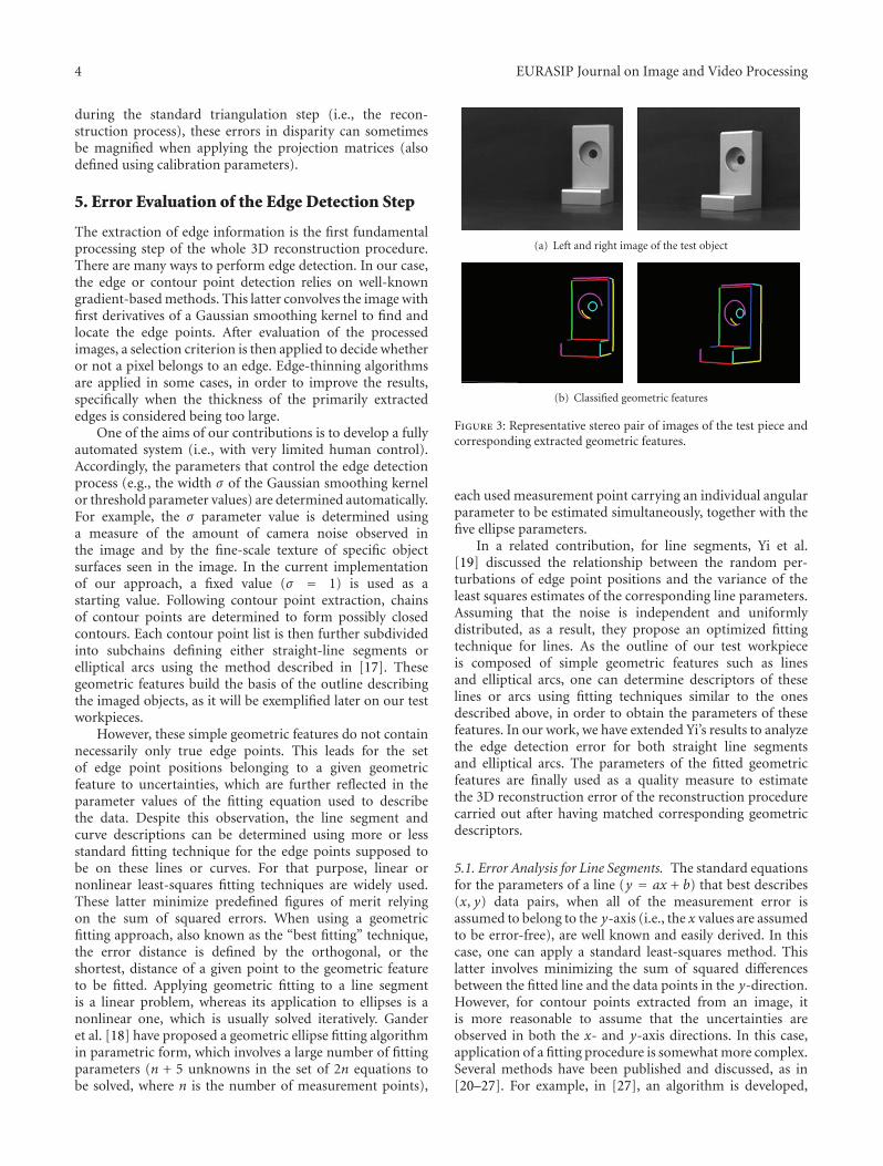
(a) Left and right image of the test object

(b) Classified geometric features

Figure 3: Representative stereo pair of images of the test piece andcorresponding extracted geometric features.

each used measurement point carrying an individual angularparameter to be estimated simultaneously, together with thefive ellipse parameters.

In a related contribution, for line segments, Yi et al.[19] discussed the relationship between the random per-turbations of edge point positions and the variance of theleast squares estimates of the corresponding line parameters.Assuming that the noise is independent and uniformlydistributed, as a result, they propose an optimized fittingtechnique for lines. As the outline of our test workpieceis composed of simple geometric features such as linesand elliptical arcs, one can determine descriptors of theselines or arcs using fitting techniques similar to the onesdescribed above, in order to obtain the parameters of thesefeatures. In our work, we have extended Yi’s results to analyzethe edge detection error for both straight line segmentsand elliptical arcs. The parameters of the fitted geometricfeatures are finally used as a quality measure to estimatethe 3D reconstruction error of the reconstruction procedurecarried out after having matched corresponding geometricdescriptors.

5.1. Error Analysis for Line Segments. The standard equationsfor the parameters of a line (y = ax + b) that best describes(x, y) data pairs, when all of the measurement error isassumed to belong to the y-axis (i.e., the x values are assumedto be error-free), are well known and easily derived. In thiscase, one can apply a standard least-squares method. Thislatter involves minimizing the sum of squared differencesbetween the fitted line and the data points in the y-direction.However, for contour points extracted from an image, itis more reasonable to assume that the uncertainties areobserved in both the x- and y-axis directions. In this case,application of a fitting procedure is somewhat more complex.Several methods have been published and discussed, as in[20–27]. For example, in [27], an algorithm is developed,


2D error distribution(μ = 0, σ = 0.32)

0.80.40−0.4−0.8

Error (pixels)

05

101520253035404550

Nu

mbe

rof

poi

nts

(a) Error distribution for a typical horizontalline in the left image


0.80.40−0.4−0.8

Error (pixels)

0

5

10

15

20

25

30

35

40

Nu

mbe

rof

poin

ts

(b) Error distribution for a typical horizontalline in the right image


0.40−0.4−0.8

Error (pixels)

02468

1012141618

Nu

mbe

rof

poin

ts

(c) Error distribution for a typical verticalline in the left image


0.40−0.4−0.8

Error (pixels)

0

5

10

15

Nu

mbe

rof

poin

ts

(d) Error distribution for a typical verticalline in the right image

2D error distribution(μ = 0.67, σ = 0.32)

1.510.50

Error (pixels)

02468

1012141618

Nu

mbe

rof

poin

ts

(e) Error distribution for a typical ellipticalline in the left image

2D error distribution(μ = 0.69, σ = 0.46)

21.61.20.80.40

Error (pixels)

02468

1012141618

Nu

mbe

rof

poin

ts(f) Error distribution for a typical ellipticalline in the right image

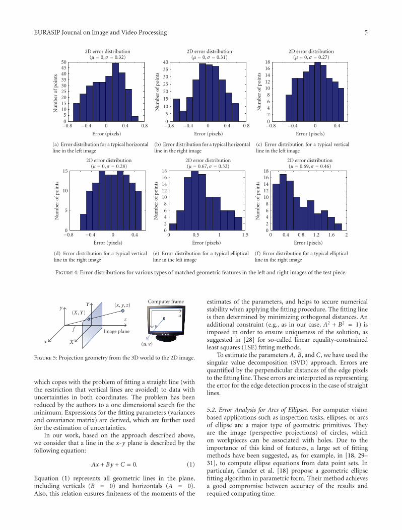
Figure 4: Error distributions for various types of matched geometric features in the left and right images of the test piece.

Computer frame

Image plane

x

y

f

z

X

Y

(X ,Y)

(x, y, z)

(u, v)

v

u

Figure 5: Projection geometry from the 3D world to the 2D image.

which copes with the problem of fitting a straight line (withthe restriction that vertical lines are avoided) to data withuncertainties in both coordinates. The problem has beenreduced by the authors to a one dimensional search for theminimum. Expressions for the fitting parameters (variancesand covariance matrix) are derived, which are further usedfor the estimation of uncertainties.

In our work, based on the approach described above,we consider that a line in the x-y plane is described by thefollowing equation:

Ax + By + C = 0. (1)

Equation (1) represents all geometric lines in the plane,including verticals (B = 0) and horizontals (A = 0).Also, this relation ensures finiteness of the moments of the

estimates of the parameters, and helps to secure numericalstability when applying the fitting procedure. The fitting lineis then determined by minimizing orthogonal distances. Anadditional constraint (e.g., as in our case, A2 + B2 = 1) isimposed in order to ensure uniqueness of the solution, assuggested in [28] for so-called linear equality-constrainedleast squares (LSE) fitting methods.

To estimate the parameters A, B, and C, we have used thesingular value decomposition (SVD) approach. Errors arequantified by the perpendicular distances of the edge pixelsto the fitting line. These errors are interpreted as representingthe error for the edge detection process in the case of straightlines.

5.2. Error Analysis for Arcs of Ellipses. For computer visionbased applications such as inspection tasks, ellipses, or arcsof ellipse are a major type of geometric primitives. Theyare the image (perspective projections) of circles, whichon workpieces can be associated with holes. Due to theimportance of this kind of features, a large set of fittingmethods have been suggested, as, for example, in [18, 29–31], to compute ellipse equations from data point sets. Inparticular, Gander et al. [18] propose a geometric ellipsefitting algorithm in parametric form. Their method achievesa good compromise between accuracy of the results andrequired computing time.


In this approach, an ellipse in a general position isexpressed in parametric form as follows:

XY =⎡⎣Ox

Oy

⎤⎦ +Q(∝)

⎡⎣a cosϕ

b sinϕ

⎤⎦, (2)

where

Q(α) =⎛⎝cosα − sinα

sinα cosα

⎞⎠. (3)

XY are the vectors [x y]T and describe the set of pointsto be fitted, O[Ox Oy]

T is the center of the ellipse, a and bare, respectively, the semimajor and the semiminor ellipseaxis (assuming b < a) and α is the angle between the x-axisand the major axis of the ellipse.

Even though the ellipse could also have been described bythe canonical equation ax2 + bxy + cy2 + dx + ey + f = 0,the description given by (2) is preferred, as it leads to moreefficient implementations of the fitting procedure.

Ellipse fitting is performed using a nonlinear least-squares approach, minimizing the squared sum of orthog-onal distances of the points to the fitting ellipse. That impliesminimizing the following criterion:

F =⎡⎣xy

⎤⎦−

⎡⎣Ox

Oy

⎤⎦−Q(∝)

⎡⎣a cosϕi

b sinϕi

⎤⎦, (4)

where i = 1, . . . ,n; and ϕi(0, . . . , 2π) are the n uniformlydistributed unknown angles associated with the set of pointsto be fitted.

Here also, the sum of orthogonal distances is interpretedas representing the error for the edge detection process in thecase of ellipses.

5.3. 2D Error Propagation. The error estimates, based on thedistances computed as described in the previous section, arethen propagated up to the 3D reconstruction step.

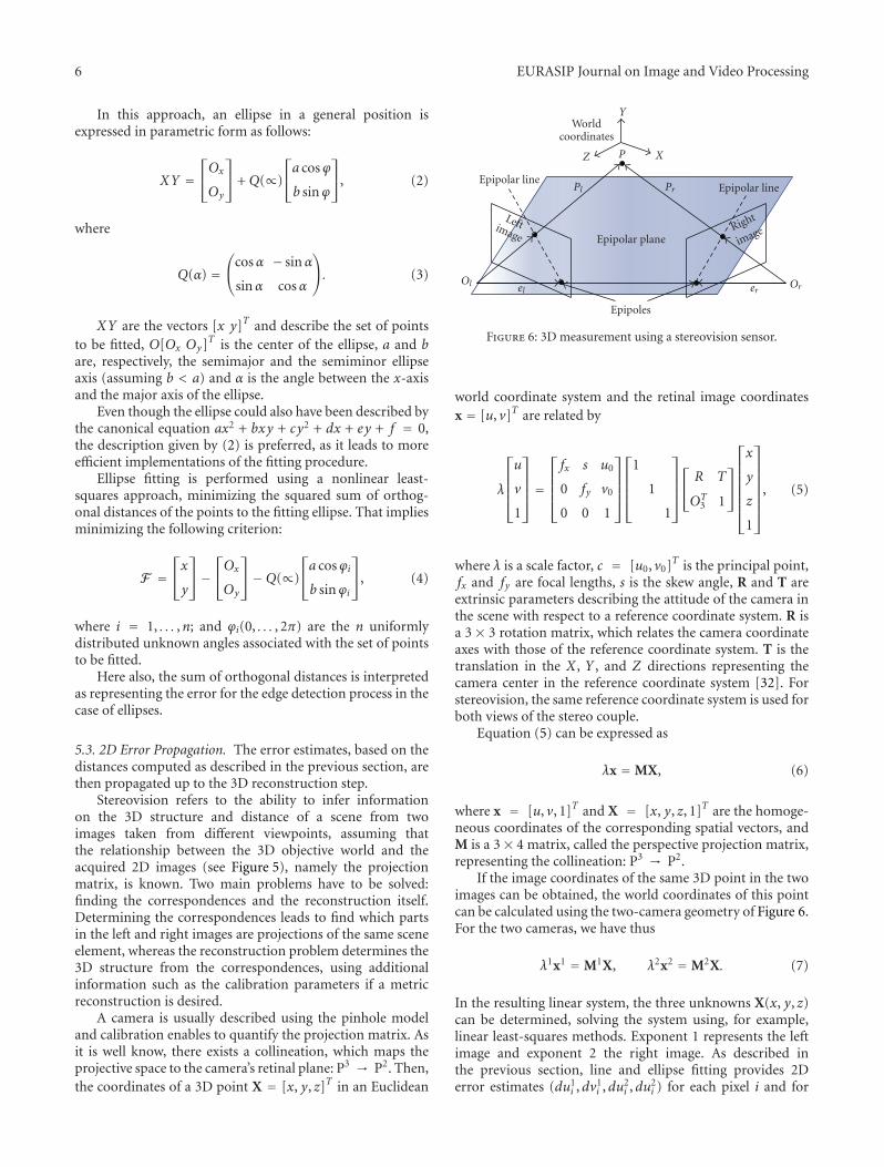
Stereovision refers to the ability to infer informationon the 3D structure and distance of a scene from twoimages taken from different viewpoints, assuming thatthe relationship between the 3D objective world and theacquired 2D images (see Figure 5), namely the projectionmatrix, is known. Two main problems have to be solved:finding the correspondences and the reconstruction itself.Determining the correspondences leads to find which partsin the left and right images are projections of the same sceneelement, whereas the reconstruction problem determines the3D structure from the correspondences, using additionalinformation such as the calibration parameters if a metricreconstruction is desired.

A camera is usually described using the pinhole modeland calibration enables to quantify the projection matrix. Asit is well know, there exists a collineation, which maps theprojective space to the camera’s retinal plane: P3 → P2. Then,the coordinates of a 3D point X = [x, y, z]T in an Euclidean

Worldcoordinates

Epipolar lineEpipolar line

Right

imageLeftimage Epipolar plane

Epipoles

X

Y

Z

Ol el er Or

P

Pl Pr

Figure 6: 3D measurement using a stereovision sensor.

world coordinate system and the retinal image coordinatesx = [u, v]T are related by

λ

⎡⎢⎢⎢⎣

u

v

1

⎤⎥⎥⎥⎦ =

⎡⎢⎢⎢⎣

fx s u0

0 fy v0

0 0 1

⎤⎥⎥⎥⎦

⎡⎢⎢⎢⎣

1

1

1

⎤⎥⎥⎥⎦

⎡⎣ R T

OT3 1

⎤⎦

⎡⎢⎢⎢⎢⎢⎢⎣

x

y

z

1

⎤⎥⎥⎥⎥⎥⎥⎦

, (5)

where λ is a scale factor, c = [u0, v0]T is the principal point,fx and fy are focal lengths, s is the skew angle, R and T areextrinsic parameters describing the attitude of the camera inthe scene with respect to a reference coordinate system. R isa 3× 3 rotation matrix, which relates the camera coordinateaxes with those of the reference coordinate system. T is thetranslation in the X , Y , and Z directions representing thecamera center in the reference coordinate system [32]. Forstereovision, the same reference coordinate system is used forboth views of the stereo couple.

Equation (5) can be expressed as

λx = MX, (6)

where x = [u, v, 1]T and X = [x, y, z, 1]T are the homoge-neous coordinates of the corresponding spatial vectors, andM is a 3× 4 matrix, called the perspective projection matrix,representing the collineation: P3 → P2.

If the image coordinates of the same 3D point in the twoimages can be obtained, the world coordinates of this pointcan be calculated using the two-camera geometry of Figure 6.For the two cameras, we have thus

λ1x1 = M1X, λ2x2 = M2X. (7)

In the resulting linear system, the three unknowns X(x, y, z)can be determined, solving the system using, for example,linear least-squares methods. Exponent 1 represents the leftimage and exponent 2 the right image. As described inthe previous section, line and ellipse fitting provides 2Derror estimates (du1

i ,dv1i ,du2

i ,du2i ) for each pixel i and for


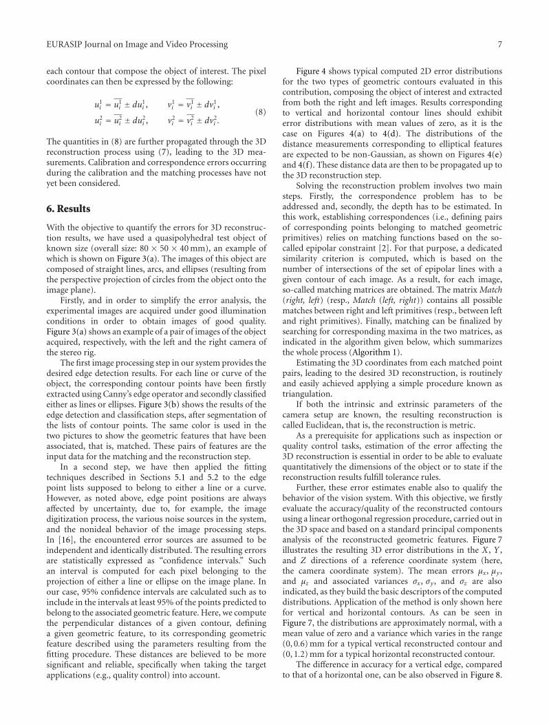
each contour that compose the object of interest. The pixelcoordinates can then be expressed by the following:

u1i = u1

i ± du1i , v1

i = v1i ± dv1

i ,

u2i = u2

i ± du2i , v2

i = v2i ± dv2

i .(8)

The quantities in (8) are further propagated through the 3Dreconstruction process using (7), leading to the 3D mea-surements. Calibration and correspondence errors occurringduring the calibration and the matching processes have notyet been considered.

6. Results

With the objective to quantify the errors for 3D reconstruc-tion results, we have used a quasipolyhedral test object ofknown size (overall size: 80 × 50 × 40 mm), an example ofwhich is shown on Figure 3(a). The images of this object arecomposed of straight lines, arcs, and ellipses (resulting fromthe perspective projection of circles from the object onto theimage plane).

Firstly, and in order to simplify the error analysis, theexperimental images are acquired under good illuminationconditions in order to obtain images of good quality.Figure 3(a) shows an example of a pair of images of the objectacquired, respectively, with the left and the right camera ofthe stereo rig.

The first image processing step in our system provides thedesired edge detection results. For each line or curve of theobject, the corresponding contour points have been firstlyextracted using Canny’s edge operator and secondly classifiedeither as lines or ellipses. Figure 3(b) shows the results of theedge detection and classification steps, after segmentation ofthe lists of contour points. The same color is used in thetwo pictures to show the geometric features that have beenassociated, that is, matched. These pairs of features are theinput data for the matching and the reconstruction step.

In a second step, we have then applied the fittingtechniques described in Sections 5.1 and 5.2 to the edgepoint lists supposed to belong to either a line or a curve.However, as noted above, edge point positions are alwaysaffected by uncertainty, due to, for example, the imagedigitization process, the various noise sources in the system,and the nonideal behavior of the image processing steps.In [16], the encountered error sources are assumed to beindependent and identically distributed. The resulting errorsare statistically expressed as “confidence intervals.” Suchan interval is computed for each pixel belonging to theprojection of either a line or ellipse on the image plane. Inour case, 95% confidence intervals are calculated such as toinclude in the intervals at least 95% of the points predicted tobelong to the associated geometric feature. Here, we computethe perpendicular distances of a given contour, defininga given geometric feature, to its corresponding geometricfeature described using the parameters resulting from thefitting procedure. These distances are believed to be moresignificant and reliable, specifically when taking the targetapplications (e.g., quality control) into account.

Figure 4 shows typical computed 2D error distributionsfor the two types of geometric contours evaluated in thiscontribution, composing the object of interest and extractedfrom both the right and left images. Results correspondingto vertical and horizontal contour lines should exhibiterror distributions with mean values of zero, as it is thecase on Figures 4(a) to 4(d). The distributions of thedistance measurements corresponding to elliptical featuresare expected to be non-Gaussian, as shown on Figures 4(e)and 4(f). These distance data are then to be propagated up tothe 3D reconstruction step.

Solving the reconstruction problem involves two mainsteps. Firstly, the correspondence problem has to beaddressed and, secondly, the depth has to be estimated. Inthis work, establishing correspondences (i.e., defining pairsof corresponding points belonging to matched geometricprimitives) relies on matching functions based on the so-called epipolar constraint [2]. For that purpose, a dedicatedsimilarity criterion is computed, which is based on thenumber of intersections of the set of epipolar lines with agiven contour of each image. As a result, for each image,so-called matching matrices are obtained. The matrix Match(right, left) (resp., Match (left, right)) contains all possiblematches between right and left primitives (resp., between leftand right primitives). Finally, matching can be finalized bysearching for corresponding maxima in the two matrices, asindicated in the algorithm given below, which summarizesthe whole process (Algorithm 1).

Estimating the 3D coordinates from each matched pointpairs, leading to the desired 3D reconstruction, is routinelyand easily achieved applying a simple procedure known astriangulation.

If both the intrinsic and extrinsic parameters of thecamera setup are known, the resulting reconstruction iscalled Euclidean, that is, the reconstruction is metric.

As a prerequisite for applications such as inspection orquality control tasks, estimation of the error affecting the3D reconstruction is essential in order to be able to evaluatequantitatively the dimensions of the object or to state if thereconstruction results fulfill tolerance rules.

Further, these error estimates enable also to qualify thebehavior of the vision system. With this objective, we firstlyevaluate the accuracy/quality of the reconstructed contoursusing a linear orthogonal regression procedure, carried out inthe 3D space and based on a standard principal componentsanalysis of the reconstructed geometric features. Figure 7illustrates the resulting 3D error distributions in the X , Y ,and Z directions of a reference coordinate system (here,the camera coordinate system). The mean errors μx, μy ,and μz and associated variances σx, σy , and σz are alsoindicated, as they build the basic descriptors of the computeddistributions. Application of the method is only shown herefor vertical and horizontal contours. As can be seen inFigure 7, the distributions are approximately normal, with amean value of zero and a variance which varies in the range(0, 0.6) mm for a typical vertical reconstructed contour and(0, 1.2) mm for a typical horizontal reconstructed contour.

The difference in accuracy for a vertical edge, comparedto that of a horizontal one, can be also observed in Figure 8.


3D error distribution in theX direction (μx = 0, σx = 0.89∗10−3)

×10−3210−1−2−3−4

Error (mm)

0

10

20

30

40

50

60

Nu

mbe

rof

poin

ts

(a) 3D error distribution in the x-direction(vertical contour)

3D error distribution in theY direction (μy = 0, σy = 0.049)

0.150.10.050−0.05−0.1

Error (mm)

05

1015202530354045

Nu

mbe

rof

poin

ts

(b) 3D error distribution in the y-direction(vertical contour)

3D error distribution in theZ direction (μz = 0, σz = 0.26)

0.40−0.4−0.8

Error (mm)

05

1015202530354045

Nu

mbe

rof

poin

ts

(c) 3D error distribution in the z-direction(vertical contour)

3D error distribution in theX direction (μx = 0, σx = 0.13)

0.30.1−0.1−0.3

Error (mm)

0

2

4

6

8

10

12

Nu

mbe

rof

poin

ts

(d) 3D error distribution in the x-direction(horizontal contour)

3D error distribution in theY direction (μy = 0, σy = 0.51)

10.60.2−0.2−0.6−1

Error (mm)

00.5

11.5

22.5

33.5

44.5

5

Nu

mbe

rof

poin

ts

(e) 3D error distribution in the y-direction(horizontal contour)

3D error distribution in theZ direction (μz = 0, σz = 1.27)

210−1−2

Error (mm)

00.5

11.5

22.5

33.5

44.5

5

Nu

mbe

rof

poin

ts(f) 3D error distribution in the z-direction(horizontal contour)

Figure 7: 3D error distribution in the x, y, and z-directions of a typical vertical and horizontal reconstructed contour.

(1) Estimation of the epipolar geometry(2) Determination of the candidate matches

(a) For each left primitive, computation of the numberof intersections of epipolar lines with right primitives.The result is the matrix Match (left, right).

(b) For each right primitive, computation of the numberof intersections of epipolar line with left primitivesin the other image. The result is the matrixMatch (right, left).

(3) Finalization/validation of the matches(c) Computation of the similarity criterion between the

two matrices: searching for corresponding maximain the two matrices.

(d) Elimination of the matched contours according tostep (c) in the two matrices.

(e) Repeat steps (a) to (d) until all contours have beenprocessed.

Algorithm 1: Matching procedure.

Thus, the quality of reconstructed vertical contours is betterthan that for horizontal ones. This observation can be tracedback to the matching problem. As a matter of fact, verticalcontours are easier to match accurately than horizontal ones,due to the configuration of the cameras of the stereo rig.

Usually, the optical axes of the cameras are not aligned, thatis, parallel, as it is the case for the geometry used whenrectifying a stereo pair of images.

Such a configuration could be obtained by rotating thecameras from their original positions to reach alignment. Analternative is accordingly needed to rectify the stereo pairof images. As a result, matched image points correspondingto point features in a rectified image pair will lie onthe same horizontal scanline and differ only in horizontaldisplacement. This horizontal displacement or disparitybetween rectified feature points is directly related to thedepth of the 3D feature point. Further, the rectifying processdoes not require a high computation cost.

Work is currently being devoted to enhance the over-all performance of the matching procedure. As couldbe expected (the behavior being routinely observed forstereovision-based reconstruction procedures), the error inthe Z direction (i.e., range) is much higher than that inthe X and Y directions (corresponding approximately tothe directions of the coordinate axes of the image plane).This behavior is induced by the vergence of the cameras.Indeed, controlling the vergence of the optical axes of thecameras defines a basic tool to obtain good results whenapplying a matching algorithm, because the disparity valuesrelated to the object of interest can be reduced. Knowledge ofthe vergence also allows a distance measure of the so-calledfixation point (defined as the intersection point between


Propagated 3D errorin the X direction

0.120.080.040

Error (mm)

0

5

10

15

20

25

30

35N

um

ber

ofpo

ints

(a) Propagated 3D error distribution (x-direction) (vertical contour)

Propagated 3D errorin the Y direction

0.60.040.020

Error (mm)

0

5

10

15

20

25

30

35

40

Nu

mbe

rof

poin

ts

(b) Propagated 3D error distribution (y-direction) (vertical contour)

Propagated 3D errorin the Z direction

0.20.160.120.080.040

Error (mm)

0

5

10

15

20

25

30

35

40

Nu

mbe

rof

poin

ts

(c) Propagated 3D error distribution (z-direction) (vertical contour)


0.30.20.10

Error (mm)

0

20

40

60

80

100

120

140

Nu

mbe

rof

poin

ts

(d) Propagated 3D error distribution (x-direction) (horizontal contour)


0.160.120.080.040

Error (mm)

0

10

20

30

40

50

60

Nu

mbe

rof

poin

ts

(e) Propagated 3D error distribution (y-direction) (horizontal contour)


1.41.210.80.60.40.20

Error (mm)

0

10

20

30

40

50

60

7080

Nu

mbe

rof

poin

ts(f) Propagated 3D error distribution (z-direction) (horizontal contour)


0.30.20.10

Error (mm)

0

2

4

6

8

10

12

14

Nu

mbe

rof

poin

ts

(g) Propagated 3D error distribution (x-direction) (elliptical contour)


0.250.20.150.10.050

Error (mm)

0

5

10

15

Nu

mbe

rof

poin

ts

(h) Propagated 3D error distribution (y-direction) (elliptical contour)


1.81.61.41.210.80.60.40.2

Error (mm)

0

2

4

6

8

10

12

14

Nu

mbe

rof

poin

ts

(i) Propagated 3D error distribution (z-direction) (elliptical contour)

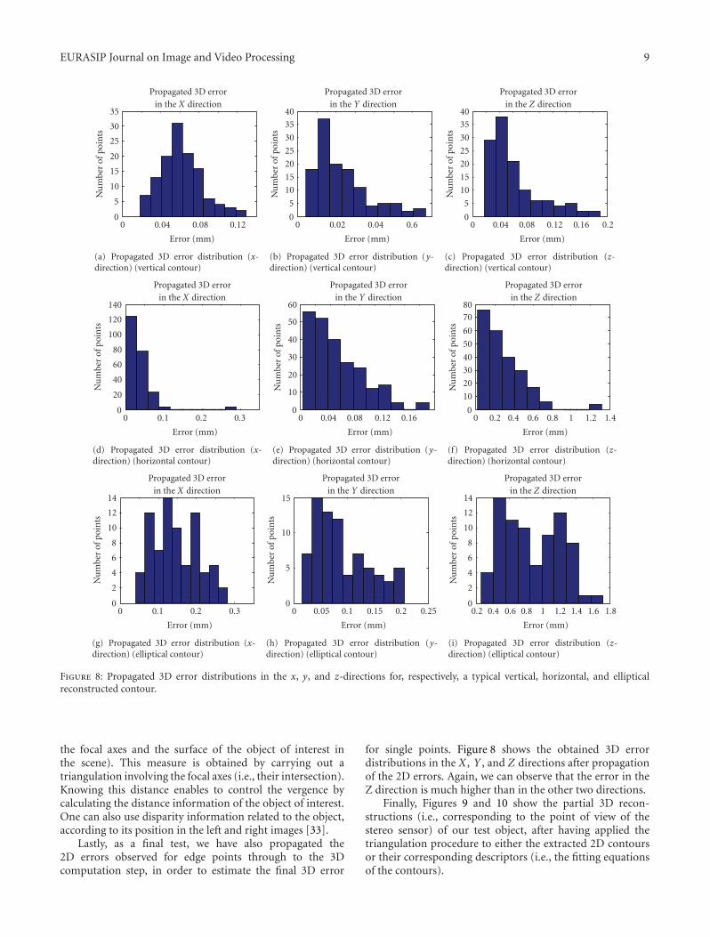
Figure 8: Propagated 3D error distributions in the x, y, and z-directions for, respectively, a typical vertical, horizontal, and ellipticalreconstructed contour.

the focal axes and the surface of the object of interest inthe scene). This measure is obtained by carrying out atriangulation involving the focal axes (i.e., their intersection).Knowing this distance enables to control the vergence bycalculating the distance information of the object of interest.One can also use disparity information related to the object,according to its position in the left and right images [33].

Lastly, as a final test, we have also propagated the2D errors observed for edge points through to the 3Dcomputation step, in order to estimate the final 3D error

for single points. Figure 8 shows the obtained 3D errordistributions in the X , Y , and Z directions after propagationof the 2D errors. Again, we can observe that the error in theZ direction is much higher than in the other two directions.

Finally, Figures 9 and 10 show the partial 3D recon-structions (i.e., corresponding to the point of view of thestereo sensor) of our test object, after having applied thetriangulation procedure to either the extracted 2D contoursor their corresponding descriptors (i.e., the fitting equationsof the contours).


−40−30−20−100102030

Y (mm)

−200

200

Z(m

m)

0

10

20

30

40

50

60

70

80

90

X(m

m)

Figure 9: Partial 3D reconstruction using actually extracted con-tours.

−40−30−20−100102030

Y (mm)

−200

200

Z(m

m)

−10

0

10

20

30

40

50

60

70

80

90

X(m

m)

Figure 10: Partial 3D reconstruction using the fitting equationsapproximating the contours.

The reconstruction using the descriptors shows that theobject is better estimated, as the reconstruction step allowsrecovering parts of contours, which have not been extractedadequately (this is especially the case for the elliptical partsof the object). In Figure 11, an example of a reconstructed3D vertical contour is shown, together with associated errorsbounds drawn as ellipses. As an example, the 3D errors areshown for one contour, which is the vertical line represented

8070

6050

4030

2010

0

X (mm)

−35.8

−35.4

−35

−34.6

Y (mm)

14

14.5

15

15.5

Z(m

m)

Figure 11: Example of a reconstructed 3D contour and associatederror bounds drawn as ellipses; the line corresponds to the verticalline represented in blue in Figure 3(b).

in blue in Figure 3(b), in order to illustrate the method. The2D ellipses around the contour represent the errors in the z-and y-directions. Since these errors are not the same for allpoints along the line, the two axes of the ellipse are different,depending on the position along the line. The reason forthis change in error magnitude can be traced back to theperpendicular distance of the pixels belonging to the edgedescribed as a line after the fitting step. We recall that thisdistance can be interpreted as representing the error resultingfrom the edge detection process for the case of straight lineprimitives, which cannot basically be assumed to be of thesame magnitude.

7. Conclusions and Outlook

In this paper, we have introduced a method for analyzingand evaluating the uncertainties encountered during vision-based reconstruction tasks. Specifically, the uncertaintieshave been estimated from the feature extraction step upto the triangulation based 3D reconstruction embeddedwithin a cognitive stereovision system. As a result, thereconstruction process is sensitive to various types of errorsources, as indicated in [16]. In this paper, we have mainlyconsidered the errors introduced by the image segmentationprocedure, their estimates being propagated through thewhole reconstruction procedure.

Approximating the contours point lists describing thepiece under evaluation using fitting results, assuming furtherthat the various errors, specifically those related to imageprocessing, are independent and identically distributed, wehave estimated error bounds for the edges detection process.These errors are defined as being equal to the orthogonaldistances of the contour pixels to the geometric featuredescribed by the corresponding fitting parameters. Thesedata are computed for each geometric feature being part ofthe object of interest. Using a dedicated error propagationscheme, the estimates have also been propagated through


the whole processing chain setup for analyzing the imagesacquired with our stereovision system.

Since the resulting 3D reconstruction depends on imagequality, the experimental images are usually acquired undergood illumination conditions, in order to obtain images ofsufficient quality using, for example, the approach describedin [14]. Controlling the acquisition conditions allows mini-mizing the 3D measurement error. The experimental resultspresented here validate the error estimation technique andshow that reconstructions of good quality with reasonableaccuracy can be automatically computed. In comparisonwith previously obtained results, the measures presentedabove, with our suggested error propagation scheme, are ofmuch higher precision and lead to reduced 3D reconstruc-tion errors.

Generalization of the error propagation scheme is cur-rently in progress in order to take into account all the othersources of errors, more specifically the matching errors.

References

[1] R. Khemmar, A. Lallement, and E. Hirsch, “Steps towardsan intelligent self-reasoning system for the automated vision-based evaluation of manufactured parts,” in Proceedings of theWorkshop on Applications of Computer Vision, in Conjunctionwith European Conference on Computer Vision (ECCV ’06), pp.136–143, Graz, Austria, May 2006.

[2] B. A. Far, S. Kohler, and E. Hirsch, “3D reconstruction ofmanufactured parts using bi-directional stereovision-basedcontour matching and comparison of real and syntheticimages,” in Proceedings of the 9th IAPR Conference on MachineVision Applications, pp. 456–459, Tsukuba Science City, Japan,May 2005.

[3] S. Kohler, B. A. Far, and E. Hirsch, “Dynamic (re)planningof 3D automated reconstruction using situation graph treesand illumination adjustment,” in Quality Control by ArtificialVision, vol. 6356 of Proceedings of SPIE, p. 11, Le Creusot,France, May 2007.

[4] R. Khemmar, A. Lallement, and E. Hirsch, “Design of anintelligent self-reasoning system for the automated vision-based evaluation of manufactured parts,” in proceedings of 7thInternational Conference on Quality Control by Artificial Vision(QCAV ’05), pp. 241–246, Nagoya, Japan, May 2005.

[5] S. D. Blostein and T. S. Huang, “Error analysis in stereodetermination of 3D point positions,” IEEE Transactions onPattern Analysis and Machine Intelligence, vol. 9, no. 6, pp. 752–765, 1987.

[6] Z. Yang and Y.-F. Wang, “Error analysis of 3D shape construc-tion from structured lighting,” Pattern Recognition, vol. 29, no.2, pp. 189–206, 1996.

[7] R. S. Ramakrishna and B. Vaidvanathan, “Error analysisin stereo vision,” in Proceedings of the Asian Conference onComputer Vision (ACCV ’98), vol. 1351, pp. 296–304, 1998.

[8] G. Kamberova and R. Bajcsy, “Precision of 3D points recon-structed from stereo,” Tech. Rep., Department of Computer &Information Science, 1997.

[9] R. Balasuramanian, D. Sukhendu, and K. Swaminathan,“Error analysis in reconstruction of a line in 3D from twoarbitrary perspective views,” International Journal of ComputerVision and Mathematicss, vol. 78, pp. 191–212, 2000.

[10] A. H. Rivera-Rios, F.-L. Shih, and M. Marefat, “Stereocamera pose determination with error reduction and tolerance

satisfaction for dimensional measurements,” in Proceedings ofthe IEEE International Conference on Robotics and Automation,pp. 423–428, Barcelona, Spain, 2005.

[11] S.-Y. Park and M. Subbarao, “A multiview 3D modelingsystem based on stereo vision techniques,” Machine Vision andApplications, vol. 16, no. 3, pp. 148–156, 2005.

[12] B. Albouy, E. Koenig, S. Treuillet, and Y. Lucas, “Accurate3D structure measurements from two uncalibrated views,”Advanced Concepts for Intelligent Vision Systems, vol. 4179, pp.1111–1121, 2006.

[13] Y. Jianxi, L. Jianting, and S. Zhendong, “Calibrating methodand systematic error analysis on binocular 3D positionsystem,” in Proceedings of the 6th International Conference onAutomation and Logistics, pp. 2310–3214, Qingdao, China,September 2008.

[14] A. Belhaoua, S. Kohler, and E. Hirsch, “Determination ofoptimal lighting position in view of 3D reconstruction errorminimization,” in Proceedings of the 10th European Congressof International Society of Stereology (ISS ’09), pp. 408–414,Bologna, Italy, June 2009.

[15] G. Egnal, M. Mintz, and R. P. Wildes, “A stereo confidencemetric using single view imagery with comparison to fivealternative approaches,” Image and Vision Computing, vol. 22,no. 12, pp. 943–957, 2004.

[16] A. Belhaoua, S. Kohler, and E. Hirsch, “Estimation of 3dreconstruction errors in a stereo-vision system,” in ModelingAspects in Optical Metrology II, vol. 7390 of Proceedings of theSPIE, pp. 1–10, Optical Metrology, Munich, Germany, June2009.

[17] C. Daul, Construction et utilisation de liste de primitives en vued’une analyse dimensionnelle de piece a geometrie simple, Ph.D.thesis, Universite Louis Pasteur, Strasbourg, France, 1989.

[18] W. Gander, G. H. Golub, and R. Strebel, “Least-squares fittingof circles and ellipses,” BIT Numerical Mathematics, vol. 34,no. 4, pp. 558–578, 1994.

[19] S. Yi, R. M. Haralick, and L. G. Shapiro, “Error propagation inmachine vision,” Machine Vision and Applications, vol. 7, no.2, pp. 93–114, 1994.

[20] D. York, “Least-squares fitting of a straight line,” CanadianJournal of Physics, vol. 44, pp. 1079–1086, 1966.

[21] M. Lybanon, “A better least-squares method when bothvariables have uncertainties,” American Journal of Physics, vol.52, pp. 22–26, 1984.

[22] B. C. Reed, “Linear least-squares fits with error in bothcoordinates,” American Journal of Physics, vol. 58, pp. 642–646,1989.

[23] A. G. Gonzalez, A. Marquez, and J. F. Sanz, “An iterativealgorithm for consistent and unbiased estimation of linearregression parameters when there are errors in both the x andy variables,” Computers and Chemistry, vol. 16, no. 1, pp. 25–27, 1992.

[24] J. R. Macdonald and W. J. Thompson, “Least-squares fittingwhen both variables contain errors : pitfalls and possibilities,”American Journal of Physics, vol. 60, pp. 66–73, 1992.

[25] B. C. Reed, “Linear least-squares fits with errors in bothcoordinates. II: comments on parameter variances,” AmericanJournal of Physics, vol. 60, pp. 59–62, 1992.

[26] D. York, N. M. Evensen, M. L. Martınez, and J. De BasabeDelgado, “Unified equations for the slope, intercept, andstandard errors of the best straight line,” American Journal ofPhysics, vol. 72, no. 3, pp. 367–375, 2004.

[27] M. Krystek and M. Anton, “A weighted total least-squaresalgorithm for fitting a straight line,” Measurement Science andTechnology, vol. 18, no. 11, pp. 3438–3442, 2007.


[28] S. Van Huffel and J. Vandewalle, The Total Least SquaresProblem, Computational Aspects and Analysis, Society forIndustrial and Applied Mathematics, Philadelphia, Pa, USA,1990.

[29] R. Halir and J. Flusser, “Numerically stable direct least squaresfitting of ellipses,” in Proceedings of the 6th InternationalConference in Central Europe on Computer Graphics and Visu-alization (WSCG ’98), pp. 125–132, Plzen, Czech, February1998.

[30] S. J. Ahn, W. Rauh, and M. Recknagel, “Ellipse fitting andparameter assessment of circular object targets for robotvision,” in Proceedings of the International Conference onIntelligent Robots and Systems, vol. 1, pp. 525–530, Kyongju,Korea, October 1999.

[31] P. O’Leary and P. Zsombor-Murray, “Direct and specific least-square fitting of hyperbolæ and ellipses,” Journal of ElectronicImaging, vol. 13, no. 3, pp. 492–503, 2004.

[32] J.-Y. Bouguet, Visual methods for three-dimensional modeling,Ph.D. thesis, California Institute of Technology, Pasadena,Calif, USA, 1999.

[33] K.-C. Kwon, Y.-T. Lim, N. Kim, Y.-J. Song, and Y.-S. Choi,“Vergence control of binocular stereoscopic camera usingdisparity information,” Journal of the Optical Society of Korea,vol. 13, no. 3, pp. 379–385, 2009.

Error Evaluation in a Stereovision-Based 3D Reconstruction System

Documents

Transcript of Error Evaluation in a Stereovision-Based 3D Reconstruction System