Fuzzy Cognitive Maps for stereovision matching

Pattern Recognition 39 (2006) 2101–2114www.elsevier.com/locate/patcog

Fuzzy Cognitive Maps for stereovision matching

Gonzalo Pajaresa,∗, Jesús M. de la Cruzb

aDpto. Sistemas Informáticos y Programación, SpainbDpto. Arquitectura de Computadores y Automática, Facultad de Informática.- Universidad Complutense, 28040 Madrid, Spain

Received 15 July 2005; received in revised form 1 February 2006; accepted 3 April 2006

Abstract

This paper outlines a method for solving the stereovision matching problem using edge segments as the primitives. In stereovisionmatching the following constraints are commonly used: epipolar, similarity, smoothness, ordering and uniqueness. We propose a newmatching strategy under a fuzzy context in which such constraints are mapped. The fuzzy context integrates both Fuzzy Clustering andFuzzy Cognitive Maps. With such purpose a network of concepts (nodes) is designed, each concept represents a pair of primitives tobe matched. Each concept has associated a fuzzy value which determines the degree of the correspondence. The goal is to achieve highperformance in terms of correct matches. The main findings of this paper are reflected in the use of the fuzzy context that allows buildingthe network of concepts where the matching constraints are mapped. Initially, each concept value is loaded via the Fuzzy Clustering andthen updated by the Fuzzy Cognitive Maps framework. This updating is achieved through the influence of the remainder neighboringconcepts until a good global matching solution is achieved. Under this fuzzy approach we gain quantitative and qualitative matchingcorrespondences. This method works as a relaxation matching approach and its performance is illustrated by comparative analysis againstsome existing global matching methods.� 2006 Pattern Recognition Society. Published by Elsevier Ltd. All rights reserved.

Keywords: Fuzzy Cognitive Maps; Fuzzy Clustering; Relaxation; Fuzzy; Stereovision; Matching; Similarity; Smoothness; Ordering; Epipolar; Uniqueness

1. Introduction

A major portion of the research efforts of the computervision community has been directed toward the study of thethree-dimensional (3-D) structure of objects using machineanalysis of images [1]. We can view the problem of stereoanalysis as consisting of the following steps: image acquisi-tion, camera modeling, feature acquisition, image matching,depth determination and interpolation. The key step is thatof image matching, that is, the process of identifying thecorresponding points in two images that are cast by the samephysical point in 3-D space. This paper is devoted solely tothis problem.

A correspondence needs to be established between fea-tures from two images that correspond to some physical fea-ture in space. Then, provided that the position of centers

∗ Corresponding author. Tel.: +34 1 3947546; fax: +34 1 3947529.E-mail address: [email protected] (G. Pajares).

0031-3203/$30.00 � 2006 Pattern Recognition Society. Published by Elsevier Ltd. All rights reserved.doi:10.1016/j.patcog.2006.04.003

of projection, the focal length, the orientation of the opticalaxis, and the sampling interval of each camera are known,the depth can be established by triangulation.

1.1. Constraints applied in stereovision matching

Our stereo correspondence problem can be defined interms of finding pairs of true matches, namely, pairs ofedge segments in two images that are generated by thesame physical edge segment in space. These true matchesgenerally satisfy some constraints [2]: (1) epipolar, giventwo segments one in the left image and a second in theright one, if we slide one of them along a parallel directionto the epipolar line, they would intersect (overlap) (Fig. 1);(2) similarity, matched edge segments have similar localproperties or attributes; (3) smoothness, disparity values in agiven neighborhood change smoothly, except at a few depthdiscontinuities; (4) ordering, the relative position amongtwo edge-segments in the left image is preserved in the rightone for the corresponding matches; (5) uniqueness, each

http://www.elsevier.com/locate/patcog

mailto:[email protected]

2102 G. Pajares, J.M. de la Cruz / Pattern Recognition 39 (2006) 2101–2114

RI

u no

overlappingoverlapping

s

q

Epipolar line

c

zv

i j

LI

h k

2maxd

i

h

2maxd

w(j) w(i)

x x

y y

xu xz

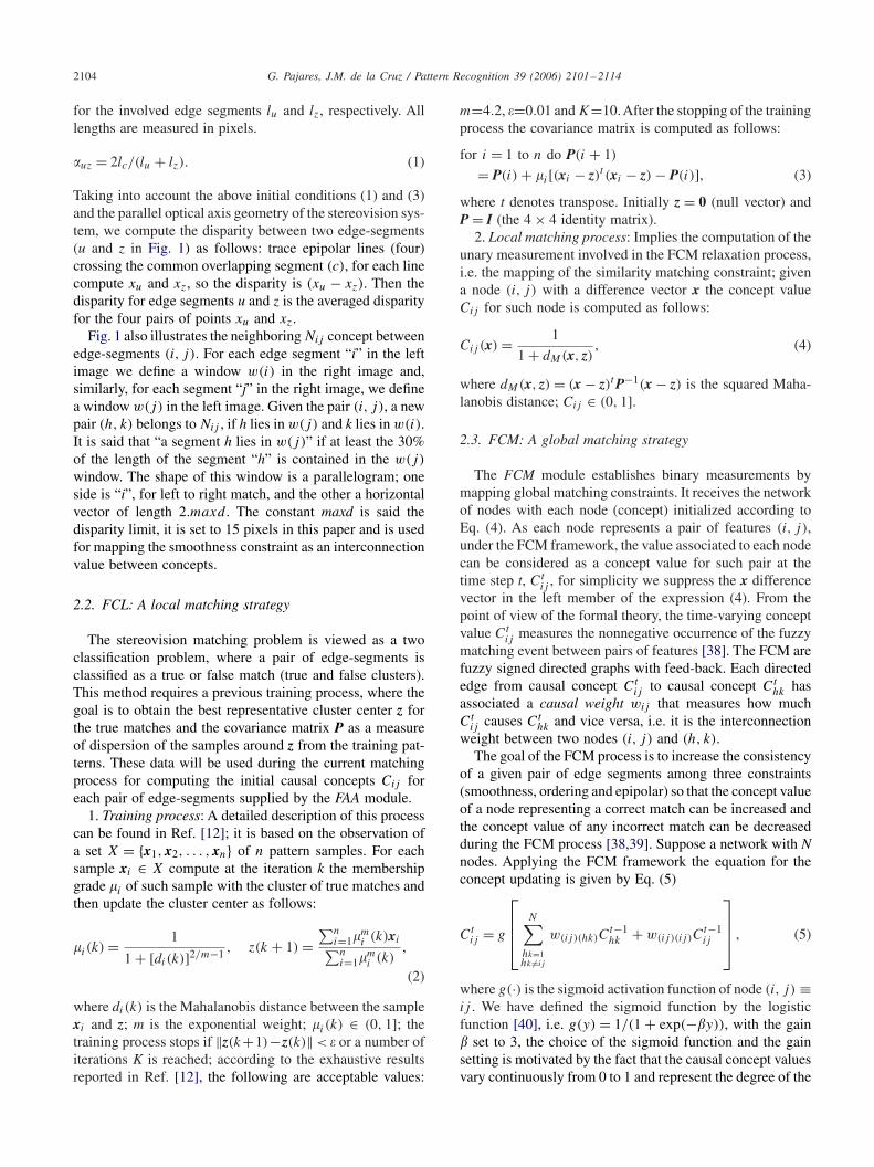
Fig. 1. Overlapping concept, edge-segments interactions and neighborhood for the pair (i, j).

edge-segment in one image should be matched to a uniqueedge-segment in the other image. The similarity and unique-ness constraints are associated to a local matching process,the smoothness and ordering constraints to a global match-ing process and the epipolar is with both, local and globalprocesses. The major difficulty of stereo processing arisesdue to the need to make global correspondences.

1.2. Techniques in stereovision matching

A review of the state-of-art in stereovision matchingallows us to distinguish two sorts of techniques broadlyused in this discipline: area-based and feature-based. Area-based stereo techniques use correlation between brightness(intensity) patterns in the local neighborhood of a pixel inone image with brightness patterns in the local neighbor-hood of the other image [2]. Feature-based methods usesets of pixels with similar attributes, normally, either pix-els belonging to edges [3,4], or the corresponding edgesthemselves [5–13]. We select a feature-based method withedge-segments as features, as they are abundant and com-monly used in indoor environments where our mobile robotequipped with the stereovision system navigates. They havebeen studied in terms of reliability [14] and robustness [15].

We have studied the performance of some local matchingstrategies: Fuzzy Clustering [12], Support Vector Machines[13], Hebbian learning [16] or a nonparametric probabilisticapproach [17]. Nevertheless, we have also verified that thebest performance in stereovision matching is achieved underglobal matching strategies [6–8]. One of the most relevantapproaches used for finding the best global matches is re-laxation; it refers to a computational mechanism involvingunary and binary measurements [18–29] with the purpose ofcomputing and improving any image unit value. Under thestereovision matching framework, the image units are thepairs of features to be matched and the values determine thestrength of the correspondences. The unary measurementsestablish an initial local correspondence by applying local

matching constraints. The binary measurements reinforceand weaken the true and false correspondences, respectivelyby applying global matching constraints through the itera-tive process involved in the relaxation process.

The following papers use a global relaxation techniquebased on probabilistic/merit [8,17–25] and optimizationthrough a Hopfield neural network [4,6,28,29].

1.3. Contribution and motivational research

The main contribution of this paper is the combination oftwo fuzzy approaches: Fuzzy Clustering (FCL) and FuzzyCognitive Maps (FCM). This strategy is justified by the fol-lowing reasons:

(a) The FCL computes the unary measurements through themapping of the similarity constraint. It has been testedfavorably in Ref. [12].

(b) The binary measurements are obtained by consideringthe consistencies between pairs of features; this can beinterpreted as fuzzy causalities in the FCM framework.

(c) The FCM works as a relaxation approach making globalcorrespondences through unary and binary measure-ments.

(d) The fuzzy causalities are obtained by mapping the globalmatching constraints, each global constraint generate akind of fuzzy causality. Different fuzzy causalities canbe combined through fuzzy aggregation operators underthe fuzzy context.

(e) The updating process is governed by an activation func-tion, which allows to control the convergence as in thewell-tested classical original cooperative algorithm pro-posed by Marr and Poggio [19].

(f) The FCM framework has been studied in terms of sta-bility [30,31].

The results obtained by our FCM relaxation method aresimilar to the obtained in Ref. [7], as this paper performs

G. Pajares, J.M. de la Cruz / Pattern Recognition 39 (2006) 2101–2114 2103

better than other existing strategies, we can conclude thatour FCM-based method works appropriately.

The performance for real-time applications is left openfor parallel implementations.

Following the FCM framework, each pair of features(edge-segments) to be matched is represented as a con-cept or node in a network. Each node has associated itsown value, which determines the strength of the correspon-dence. We use the FCL approach for computing the initialmatching estimation, i.e. the initial correspondence valuefor each pair of features. This initial value is updated by theinfluence of neighboring nodes through the mapping of thestereovision matching (local and global) constraints underthe FCM framework. The final correspondences are estab-lished based on the final nodes’ values. As in Ref. [7], weconsider the possible smoothness and ordering constraintsviolations due to occlusions, camera geometry, objects nearthe cameras, etc.

1.4. Paper organization

The paper is organized as follows. In Section 2, thefull sequential stereovision matching process is described,where the FCL and FCM frameworks are described. Theperformance of the method is illustrated in Section 3, wherea comparative study against other existing global match-ing methods is carried out. Finally in Section 4 there is adiscussion of some related topics.

2. Sequential stereovision matching process

The two cameras have equal focal lengths and are alignedso that their viewing direction is parallel. The plane formedby the viewed point and the two focal points intersects theimage plane along a horizontal line known as the epipo-lar line. A grid pattern of parallel horizontal lines is usedfor camera alignment. The cameras are adjusted so thatthe images of these lines coincide. Thus each point in anedge segment lies along the same horizontal (epipolar) linecrossing both images. This is part of the system calibrationprocess.

This paper proposes a sequential combination of fourmethods for solving the stereovision matching problem.Each method is implemented by a module. The system re-ceives as inputs a pair of stereo images left (LI) and right(RI). This pair is processed in order to extract features andattributes in the FAA module, each pair of extracted features(i, j) is to be matched, the features i and j come from LI andRI, respectively. For each pair (i, j) an attribute differencevector x is computed. All extracted x vectors are suppliedto the FCL module, which computes an initial fuzzy con-cept value Cij for each pair of features, i.e. it computesthe unary measurement. This module uses the similarityconstraint and requires a previous training process for com-puting each fuzzy concept value. Until this stage, only a

local matching process is carried out. Once all fuzzy match-ing concept values are obtained, they are supplied to theFCM module, which updates each Cij concept value takinginto account the weights interconnecting causal concepts.The FCM module implements the global matching process.After this stage, perhaps there are still ambiguous matcheswhich are solved by the unambiguous (UA) module basedon the strength of each state. The output of the system is aset of matches. We give details about the behavior of eachmodule.

2.1. Feature and attribute extraction (FAA)

The contour edges in both images are extracted using theLaplacian of Gaussian filter in accordance with the zero-crossing criterion [32]. For each zero-crossing in a givenimage, its gradient vector (magnitude and direction) [33,34],Laplacian [34] and variance [35] values are computed fromthe gray levels of a central pixel and its eight immediateneighbors. Gradient magnitude, Laplacian and variance mea-sure the focusing degree for each zero-crossing [35], i.e. thisis a kind of edginess’ measurement. The edges are obtainedby joining adjacent zero-crossings following the algorithmin Tanaka and Kak [36], where: (1) a margin of deviation of±20% in gradient magnitude and of ±45◦ in gradient direc-tion is allowed; (2) each detected contour is approximatedby a series of piecewise linear line segments [37]. Finally,for every segment, an average value of the four attributes isobtained from all computed values of its zero-crossings. Allaverage attribute values are normalized in the same range.

Each pair of features has two associated 4-dimensionalvectors xi and xj , where the components are the attributevalues, and the sub-indices i and j denote features belongingto the left and right images, respectively. A four-dimensionaldifference measurement vector x is then also obtained fromthe above xi and xj vectors, x=xi−xj ={xm, xd, xl, xv}. Thecomponents of x are the corresponding differences for mod-ule and direction gradient, Laplacian and variance values.Only those pairs verifying the following three initial condi-tions will be processed: (1) their absolute value of the differ-ence in the gradient direction is below a specific threshold,fixed to 25◦; (2) their absolute value in the gradient magni-tude is also below a fixed threshold, set to 15; and (3) theiroverlap rate surpasses a certain value, fixed to 0.5. The re-maining pairs that do not meet such conditions are directlyconsidered as false correspondences. The overlap is a con-cept introduced in Medioni and Nevatia [5], two segments uand z overlap if by sliding one of them in a direction parallelto the epipolar line, they would intersect.

Fig. 1 clarifies the overlapping concept. Indeed, segmentu in the left image overlaps with segment s in the right im-age, but segment v does not overlap with s. The overlap ratebetween edge segments (u, z), �uz is defined as the percent-age of coincidence, ranging in [0,1], when two segmentsu and z overlap, and it is computed taken into account thecommon overlap length lc defined by c and the two lengths


for the involved edge segments lu and lz, respectively. Alllengths are measured in pixels.

�uz = 2lc/(lu + lz). (1)

Taking into account the above initial conditions (1) and (3)and the parallel optical axis geometry of the stereovision sys-tem, we compute the disparity between two edge-segments(u and z in Fig. 1) as follows: trace epipolar lines (four)crossing the common overlapping segment (c), for each linecompute xu and xz, so the disparity is (xu − xz). Then thedisparity for edge segments u and z is the averaged disparityfor the four pairs of points xu and xz.

Fig. 1 also illustrates the neighboring Nij concept betweenedge-segments (i, j). For each edge segment “i” in the leftimage we define a window w(i) in the right image and,similarly, for each segment “j” in the right image, we definea window w(j) in the left image. Given the pair (i, j), a newpair (h, k) belongs to Nij , if h lies in w(j) and k lies in w(i).It is said that “a segment h lies in w(j)” if at least the 30%of the length of the segment “h” is contained in the w(j)

window. The shape of this window is a parallelogram; oneside is “i”, for left to right match, and the other a horizontalvector of length 2.maxd . The constant maxd is said thedisparity limit, it is set to 15 pixels in this paper and is usedfor mapping the smoothness constraint as an interconnectionvalue between concepts.

2.2. FCL: A local matching strategy

The stereovision matching problem is viewed as a twoclassification problem, where a pair of edge-segments isclassified as a true or false match (true and false clusters).This method requires a previous training process, where thegoal is to obtain the best representative cluster center z forthe true matches and the covariance matrix P as a measureof dispersion of the samples around z from the training pat-terns. These data will be used during the current matchingprocess for computing the initial causal concepts Cij foreach pair of edge-segments supplied by the FAA module.

1. Training process: A detailed description of this processcan be found in Ref. [12]; it is based on the observation ofa set X = {x1, x2, . . . , xn} of n pattern samples. For eachsample xi ∈ X compute at the iteration k the membershipgrade �i of such sample with the cluster of true matches andthen update the cluster center as follows:

�i (k) = 1

1 + [di(k)]2/m−1 , z(k + 1) =∑n

i=1�mi (k)xi∑n

i=1�mi (k)

,

(2)

where di(k) is the Mahalanobis distance between the samplexi and z; m is the exponential weight; �i (k) ∈ (0, 1]; thetraining process stops if ‖z(k+1)−z(k)‖ < � or a number ofiterations K is reached; according to the exhaustive resultsreported in Ref. [12], the following are acceptable values:

m=4.2, �=0.01 and K=10. After the stopping of the trainingprocess the covariance matrix is computed as follows:

for i = 1 to n do P(i + 1)

= P(i) + �i[(xi − z)t (xi − z) − P(i)], (3)

where t denotes transpose. Initially z = 0 (null vector) andP = I (the 4 × 4 identity matrix).

2. Local matching process: Implies the computation of theunary measurement involved in the FCM relaxation process,i.e. the mapping of the similarity matching constraint; givena node (i, j) with a difference vector x the concept valueCij for such node is computed as follows:

Cij (x) = 1

1 + dM(x, z), (4)

where dM(x, z) = (x − z)tP−1(x − z) is the squared Maha-lanobis distance; Cij ∈ (0, 1].

2.3. FCM: A global matching strategy

The FCM module establishes binary measurements bymapping global matching constraints. It receives the networkof nodes with each node (concept) initialized according toEq. (4). As each node represents a pair of features (i, j),under the FCM framework, the value associated to each nodecan be considered as a concept value for such pair at thetime step t, Ct

ij , for simplicity we suppress the x differencevector in the left member of the expression (4). From thepoint of view of the formal theory, the time-varying conceptvalue Ct

ij measures the nonnegative occurrence of the fuzzymatching event between pairs of features [38]. The FCM arefuzzy signed directed graphs with feed-back. Each directededge from causal concept Ct

ij to causal concept Cthk has

associated a causal weight wij that measures how muchCt

ij causes Cthk and vice versa, i.e. it is the interconnection

weight between two nodes (i, j) and (h, k).The goal of the FCM process is to increase the consistency

of a given pair of edge segments among three constraints(smoothness, ordering and epipolar) so that the concept valueof a node representing a correct match can be increased andthe concept value of any incorrect match can be decreasedduring the FCM process [38,39]. Suppose a network with Nnodes. Applying the FCM framework the equation for theconcept updating is given by Eq. (5)

Ctij = g

⎡⎢⎢⎣

N∑hk=1hk �=ij

w(ij)(hk)Ct−1hk + w(ij)(ij)C

t−1ij

⎤⎥⎥⎦ , (5)

where g(·) is the sigmoid activation function of node (i, j) ≡ij . We have defined the sigmoid function by the logisticfunction [40], i.e. g(y) = 1/(1 + exp(−�y)), with the gain� set to 3, the choice of the sigmoid function and the gainsetting is motivated by the fact that the causal concept valuesvary continuously from 0 to 1 and represent the degree of the


matching. So, the output function must cover the continuousrange from 0 to 1, moreover in order to avoid severe biasthe slope of the sigmoid function must vary smoothly.

In our stereovision matching approach the causal weightsare symmetric, i.e. the influence of causal concepts is recip-rocal. The self-feedback terms are set to the unity w(ij)(ij) =1, so the previous causal concept contributes as a factor ofstabilization during the computation of the current causalconcept against an excessive strength coming from the re-mainder neighboring causal concepts. This is because Ct−1

ij

was initially loaded from the mapping of the strong similar-ity constraint. The causal weights w(ij)(hk) take values in thefuzzy interval [−1, +1]; w(ij)(hk) =0 indicates no causality,w(ij)(hk) > 0 indicates causal increase or positive causality:Ct

ij increases as Ct−1hk increases and Ct

ij decreases as Ct−1hk

decreases; w(ij)(hk) < 0 indicates causal decrease or negativecausality: Ct

ij decreases as Ct−1hk increases and Ct

ij increases

as Ct−1hk decreases.

The FCM task is to find the most stable network configu-ration, where the concept values do not change after a num-ber of iterations. Now we map the smoothness, ordering andepipolar stereovision matching constraints under the formof causal weights in order to represent the consistency be-tween the current pair of features under correspondence andthe pairs of features in a given neighborhood. The causalweights make global consistency between neighbors pairsof edge segments based on such constraints. Based on Ref.[7] we map the constraints as causal weights as follows.

2.3.1. Mapping the smoothness constraintThe smoothness constraint assumes that neighboring edge

segments have similar disparities, except at a few depth dis-continuities [5]. Generally, when the smoothness constraintis applied, it is assumed there is a bound on the disparityrange allowed for any given segment. This limit is denotedas maxd, fixed at 15 pixels in this paper, (see Fig. 1 anddiscussion in Section 2.1).

Given “i” and “h” in w(j) and “j” and “k” in w(i) where“i” matches with “j” and “h” with “k” the differential dis-parity |dij −dhk|, measures how close the disparity betweenedge segments “i” and “j” denoted as dij is to the dispar-ity dhk between edge segments “h” and “k”. The disparitybetween edge segments is the average of the disparity be-tween the two edge segments along the length they over-lap. This differential disparity criterion is used in [4–8,29]among others. We define a compatibility coefficient derivedfrom Refs. [4,7,29] given by

c(ij)(hk)(D) = 1

1 + exp[�(D/m(D) − 1)] , (6)

where D=|dij −dhk|, m(D) denotes the average of all valuesD in the pair of stereo images (LI and LR) under process-ing. The slope of the compatibility coefficient in Eq. (6) isexpressed by � and varies for each pair of stereo images. Todetermine �, it is assumed that the probability distribution

function of D is Gaussian with average m(D) and standarddeviation �(D), i.e. p(D) = [1 + exp[�(D(ij)(hk)/m(D) −1)]]−1. Under this assumption and following [41,42], toset the possibility value to 0.1 when the value of cumu-lative distribution function is 0.9, � value is calculated by� = ln 9((m(D))/(1.282�(D))). In our experiments, typicalvalues of �, m(D) and �(D) are about 6, 9 and 2, respec-tively. So, values of D near 0 should give high values in thecompatibility coefficient c(ij)(hk)(·) ≈ +1, but near 25 theygive low values, c(ij)(hk)(·) ≈ 0. Note that c(ij)(hk)(·) rangesin (0,1). So, a compatibility coefficient of +1 is obtained fora good consistency between nodes (i, j) and (h, k)(D = 0)

and a compatibility of 0 for a bad consistency (D?0). Thiscausal weight embedding the smoothness constraint shouldindicate positive causality for high compatibility coefficientvalues and vice versa.

2.3.2. Mapping the ordering constraintWe define the ordering coefficient O(ij)(hk), for the edge-

segments according to Eq. (7), which measures the relativeaverage position of edge segments “i” and “h” in the leftimage with respect to “j” and “k” in RI, related to the neigh-boring Nij , it ranges from 0 to 1.

O(ij)(hk) = − 1

S

∑S

o(ij)(hk)

where o(ij)(hk) = ‖R(xi − xh) − R(xj − xk)| − 1|and R(r) =

{1 if r > 0,

0 otherwise.(7)

We trace S scanlines (four) along the common overlappinglength, each scanline produces a set of four intersectionpoints (iS and hS in LI and jS and kS in the RI) with the fouredge-segments. Hence, the lower-case oijhk can be com-puted as in Ref. [4] considering the above four edge pointsand it takes 0 and 1 as two discrete values. A value of +1 inthe ordering coefficient means that the ordering constraintis preserved. On the contrary, a value of 0 indicates thatthe ordering constraint is not preserved. The causal weightembedding the ordering constraint should indicate positivecausality for a high ordering coefficient value.

2.3.3. Mapping the epipolar constraint (overlappingconcept)

The epipolar constraint is mapped through the overlappingconcept in Ref. [5], by the overlapping coefficient:

�(ij)(hk) = 0.5(�ij + �hk), (8)

where � is the overlap rate defined in Eq. (1). Under theepipolar constraint we can assume that correct/incorrectmatches should have high/low overlap rates, i.e. the over-lapping coefficient should be +1 or 0, respectively and�(ij)(hk) for neighborhoods should be high increasing theconsistency. The use of the overlapping criterion is justi-fied by the fact that the edge segments are reconstructedby piecewise linear line segments as described in Section


2.1. The reasoning for the influence of this coefficient inthe causal weight is similar to the previous ones for thecompatibility and ordering coefficients.

2.3.4. Considering smoothness and ordering constraintsviolations

There are complex images in which the ordering andsmoothness constraints can be violated. In systems with par-allel geometry, objects close to the cameras, occlusions andalso the definition of a neighborhood (disparity limit) couldlead to such violations. So, some excellent neighborhoodscould be excluded.

When can we say whether or not there are violations? Theordering constraint is not violated if O(ij)(hk) > U0, with U0,set to 0.85 in this paper. The smoothness constraint is not vi-olated when: (1) the pairs (i, j) and (h, k) are to be matched,being h a neighborhood of i in w(j) and k a neighborhood ofj in w(i), Fig. 1, according to the fixed disparity limit (min-imum disparity criterion [5]); (2) the causal concept valueat time t, Ct

ij has a high positive value although it is not themaximum of all matches (h, k′) where h is involved. This isformally expressed as follows: Ct

hk �H ∗(Cthk′)max∀k′ ∈ RI

with (Cthk′)max = max{Ct

hk′ , ∀k′ ∈ RI }, H is set to 0.85 inthis paper. The compatibility coefficient is maximum if thematching states are maximum (minimum differential dispar-ity) and vice versa. When no violations occur, the compat-ibility and ordering coefficients are computed through Eqs.(6) and (7), respectively.

Depending on which of the above conditions is notfulfilled, we say that the ordering, smoothness or both areviolated. When this occurs, global consistency is not appli-cable, and we must fall back on local consistency, i.e. weonly consider isolated causal concept values without theneighboring contribution. This is to avoid that true pairs ofedge segments are not penalized during the relaxation pro-cess due to the violation of such constraints. Depending onwhich constraint is violated, the corresponding coefficient is,

v(ij)(hk) = 0.5(Ctij + Ct

hk), where v = c, O. (9)

2.3.5. Fuzzy criteria for computing the causal weightsOnce the smoothness, ordering and epipolar stereovision

matching constraints have been mapped, we have availablethe compatibility, ordering and overlapping coefficients de-rived from such constraints, respectively. Now the goal is tocombine the three coefficients, so that they can be used inthe expression (5). Making use of the fuzzy theory, we canconsider these coefficients as membership functions, whichcan be combined in order to compute the causal weightw(ij)(hk). Hence, in our approach the causal weight is con-sidered as a fuzzy measurement (membership value). Underan expert system context [43] is a common practice to use aminimum operator for combining the opinion of several ex-perts. Nevertheless, taking into account the dissertations inZimmermann [44], a straightforward approach for aggregat-ing fuzzy sets, would be to use the aggregating procedures

frequently used in multi-criteria decision theory. They re-alize the idea of trade-offs between conflicting goals whencompensation is allowed, and the resulting trade-offs liebetween the most optimistic lower bound and the mostpessimistic upper bound, that is, they map between theminimum and the maximum degree of membership of theaggregated sets. Therefore they are called averaging opera-tors. Following the discussion in Ref. [44] about the criteriafor selecting appropriate aggregation operators, we find thatadaptability is suitable; this can be achieved by parametriza-tion. Thus min and max operators cannot be adapted atall. They are acceptable in situations in which they fit, bycontrast, there are other operators that can be adapted tocertain contexts by setting their parameters; we have usedthe Hamacher’s union operator. Taking into account thatcausal weights are considered as fuzzy membership valuesand making use of the operator’s associativity Eq. (10) isderived. The parameter � allows a fitting appropriately

�(ij)(hk) = (� − 1)c(ij)(hk)O(ij)(hk) + c(ij)(hk) + O(ij)(hk)

1 + �c(ij)(hk)O(ij)(hk)

,

W(ij)(hk) = (� − 1)�(ij)(hk)�(ij)(hk) + �(ij)(hk) + �(ij)(hk)

1 + ��(ij)(hk)�(ij)(hk)

,

(10)

where ��−1, we have found acceptable the behavior of thisparameter by setting it to 1. This is because its behavior is atrade-off between maximum and minimum operators [44].We have tested other values for � and other parameterizedoperators (Einstein, Yager, Dubois and Prade among others,Zimmerman) without any apparent improvement in the finalresults.

As a result of the aggregation’s operators, the resultingW(ij)(hk) from Eq. (10) ranges in [0, +1]. So, rescaling thisinterval to [−1, +1], we can derive the final causal weightw(ij)(hk) between features (i, j) and (h, k) as required byEq. (5). So, we obtain,

w(ij)(hk) = 2W(ij)(hk) − 1. (11)

So, high coefficient values should give high causal weightsi.e. positive causality as expected and vice versa for lowcoefficient values and negative causality.

2.3.6. Full FCM processThe full FCM process can be summarized as follows:

(1) Initialization: Assume a network of N causal conceptsor nodes representing pairs of edge segments (i, j) ≡ij . Initially, at t = 0, the causal concept values Ct

ij aresupplied by the FCL module and computed accordingto Eq. (4).

(2) FCM process: Set t = t + 1 and np = 0; compute thecausal weights according to Eq. (11); update each Ct

ij

according to Eq. (5); if |Ctij −Ct−1

ij | > � then np=np+1;when all ij nodes are updated, if np �= 0 or t < tmax then


start step 2 once again, else stop. Otherwise, the networkreaches its stabilization or convergence, i.e. np = 0.

(3) Output: Ctij updated.

Where np is the number of nodes for which the matchingconcept values are modified by the updating procedure, � isa constant value to accelerate the network stabilization, setto 0.01 in our experiments.

2.3.7. Uniqueness constraintThe uniqueness constraint completes the set of matching

constraints used for solving our stereovision matching prob-lem.

A left edge segment can be assigned to a unique right edgesegment (unambiguous pair) or several right edge segments(ambiguous pairs). The decision about whether a match iscorrect is made by choosing the greater causal concept value(in the unambiguous case there is only one) whenever itsurpasses a previous fixed threshold U1(=0.5), intermediatevalue for Ct

ij ranging in [0,1]. A true match (i, j) shouldhave Ct

ij = 1.The ambiguities produced by broken edge segments are

allowed. Hence, it is possible that more than two segmentsin one image, coming from a broken edge segment, couldmatch with a unique segment in the other image. The fol-lowing pedagogical example from Fig. 1 clarifies this. Theedge segment u in LI matches with the broken segment rep-resented by s and q in RI, but under the condition that s andq do not overlap, the s and q orientations do not differ bymore than U2(= ± 10◦) and the causal concepts values forboth edge segments Ct

us and Ctuq are greater than U1.

After the disambiguation process, the resulting causal con-cept values determine the degree of matching for each pairof edge-segments.

3. Validation, comparative analysis and performanceevaluation

3.1. Design of a test strategy

In order to assess the validity and performance of the pro-posed method, we have designed the same test strategy usedin Ref. [7]. The intention is to compare the performance ofthe proposed method against the method proposed in suchreference and simultaneously against the strategies alreadyused in Ref. [7] for comparative purposes. The testing pro-cess is as follows. We have selected 82 stereo pairs of realis-tic stereo images from an indoor environment. Fig. 2 showsfour representative images of this indoor environment; eachimage is the left image of a stereo pair. All tested imagesare 512 × 512 pixels in size, with 256 gray levels. The 82stereo pairs are classified into three groups: SP1, SP2 andSP3 with 28, 31 and 23 pairs of stereo images, respectively.Each stereo pair consists of two left and right original im-ages and two left and right images of labeled edge segments.Previously, we used an additional set of 15 stereo images

to compute the cluster center z and the covariance matrix Paccording to Eqs. (2) and (3), respectively. Then, after eachstereo pair set is processed the true matches are added tothe set of training samples for updating z and P. The groupSP1 consists of stereo images without apparent complexity;Fig. 3 shows a stereo pair representative of the group SP1.

Group SP2 corresponds to scenes where a repetitive struc-ture (vertical books) has been captured; Fig. 4 shows a stereopair representative of SP2. Finally, group SP3 contains ob-jects close to the cameras, which produce a high range ofdisparity violating the smoothness and ordering constraints.Fig. 5 is a stereo pair representative of SP3, where we cansee the object labeled as 9, 10 in left image and 11, 12 inright image as a characteristic example of an object closeto the cameras occluding the edge segment 19 in the rightimage. Although this last type of images is unusual, its treat-ment is very important as they could produce fatal errorsin navigation systems for example, where the nearest ob-jects must be processed immediately. The SP2 and SP3 areof special interest as they are complex images containingstructures that appear with a high degree of difficulty. Thiskind of images have been studied in depth in Refs. [6,7,13]where similar considerations have been also introduced todeal with the violation of the smoothness and ordering con-straints. Therefore, we compare our Fuzzy Cognitive Mapsstrategy (FCMS) against the Support Simulated Annealing(SANN) in Ref. [7], but also with the method described inRef. [8] which is a Relaxation Labeling (RELB) approachand the method described in Ref. [6], which is an opti-mization approach based on the Hopfield Neural Network(HNNB1). FCMS and SANN use the same philosophy: (a)both map the similarity constraint through a local matchingstrategy, Fuzzy Clustering and Support Vector Machines, re-spectively; (b) they map the same set of global matchingconstraints through the FCM and Simulated Annealing re-laxation processes, respectively.

Both, RELB and HNNB1 apply the similarity constraintby computing a matching probability based on the estimationof a probability density function through the Bayes’s the-ory. The matching probabilities are used as the inputs for therelaxation and optimization processes, respectively. Fromthese processes, RELB performs an iteration procedure byapplying smoothness, ordering and uniqueness constraints.HNNB1 performs the optimization process by mapping thesmoothness and uniqueness in an energy function which isto be minimized. From HNNB1, we have implemented anew version HNNB2, by mapping the ordering constraint asan energy function to be minimized and applying the simi-larity constraint as the 4-dimensional difference null vectorx. HNNB2 can be considered a very close approach to thatdescribed in Ref. [4], although this work uses edge pixels asfeatures, we have modified the original method in Ref. [4]to use edge-segments as in SANN. Also, from HNNB1 wehave implemented a new version, HNNP, where the similar-ity constraint is mapped by estimating a probability densityfunction through the Parzen’s window [17].


Fig. 2. Left stereo images representative of the indoor environment.

Fig. 3. Group SP1 (a) and (b) original left and right stereo images; (c) and (d) labeled edge segments in left and right images.



We have also compared our approach with the StochasticStereovision Matching Method (SSVM) in Ref. [41], alsoused in Ref. [42]. This method uses the regularization cri-terion proposed in Ref. [45], where an energy functional isminimized based on a penalty functional which measuresthe dissimilarity between corresponding features (similar-ity constraint) and a stabilizing functional by which thesmoothness constraint is imposed. The energy minimization

is carried out through the Simulated Annealing algorithm,we have used a value of 50 as in Ref. [41] for the regular-ization parameter � (this works well for images quantizedin 8-bit values) and the same neighborhood criteria as thatused in this paper. Two differences are considered in thisimplementation with respect to our implementation: (1) theedge-segments disparities are the outputs obtained in SSVM,which are used to obtain the correspondences and (2) the


hierarchical coarse-to-fine control structure with re-heatingin Ref. [42] is not used in our implementation.

Finally we have chosen the minimum differential dispar-ity algorithm (MDDA) [5] for comparative purposes for thefollowing reasons: (1) it is a merit relaxation approach; (2) itapplies the commonly used constraints (similarity, smooth-ness and uniqueness); (3) it uses edge segments as featuresand the contrast and orientation of the features as attributes;and (4) some concepts of MDDA, such as minimum differ-ential disparity, overlapping concept, disparity limit or av-erage disparity are used in our FCMS approach. Table 1summarizes the main differences between the eight strate-gies compared. All methods use edge-segments as featuresand the same four attributes.

We have used the same set of training patterns for esti-mating z and P in FCMS and a decision function in SVSAand also the probabilities densities in RELB, HNNB1 andHNNB2. Once each set SP1, SP2 and SP3 is processed, weuse the true matches as new training patterns, which areadded to the old ones, for new estimations.

3.2. Comparative analysis

The system processes the SP1, SP2 and SP3 groups. Ofall the possible combinations of pairs of matches formed bysegments of left and right images only 643, 584 and 474pairs are considered for SP1, SP2 and SP3, respectively un-der the thresholds and settings given in Section 2.1. Thecomputed results with the thresholds and settings given inSection 2.1 are summarized in Table 2. It shows the percent-age of successes for each group (SP1, SP2 and SP3) andfor each method (FCMS, SANN, RELB, HNNB1, HNNB2,HNNP, SSVM, and MDDA) as a function of the number ofiterations. Iteration 0 corresponds to the results for the localmatching process, Fuzzy Clustering and Support Vector Ma-chines in FCMS and SANN, respectively. This is the startingpoint for the FCM process in our approach, Section 2.3.6.

Decision process: When the network stabilization hasbeen achieved or the maximum number of iterations(tmax =100) reached, there are still both unambiguous pairsof segments and ambiguous ones, depending on either one,and only one, or several right image segments correspond-ing to a given left image segment. In any case, the decisionabout whether a match is correct or not is made by choosingthe result of greater causal concept value in FCMS, greaterstate value in SANN, greater probability in RELB, HNNB1,HNNB2 and HNNP, and the best merit value for MDDA.

In the unambiguous case there is only one. The valuesmust be greater than the corresponding intermediate value:0.5 for the probabilities in RELB, HNNB1, HNNB2 andHNNP, 0 for the states in SANN and 0.5 for the causalconcept values in FCMS.

According to values from Table 2, the following conclu-sions may be inferred:

(1) Local matching process (iteration 0, still the iterationprocesses have not been triggered): The best performances

are achieved with FCMS and SANN. This means that theFCL and the Support Vector Machines appear as good lo-cal matching methods. The results obtained by HNNP arealso good. The methods without estimation (HNNB2 andMDDA) obtain the worst results at this phase.

(2) Global matching process Group SP1: The best perfor-mance is achieved with FCMS. The local matching resultsare improved through the global matching process. The or-dering constraint is not decisive: HNNB2 (with ordering)obtains worse results than HNNB1 and HNNP (without or-dering). There are no violations in the smoothness and or-dering constraints. In Ref. [7] is reported that SANN reachesits equilibrium with an average of 65 iterations, with suchnumber of iterations the performance of SANN is compara-ble to the performance of FCMS with 35 iterations. As thisassertion is also valid for groups SP1 and SP2, we can con-clude that the fuzzy causal approach under FCMs is suitablein terms of performance in stereovision matching, i.e. thecausal reasoning and decision process under a fuzzy point ofview is consistent with that of the human. This is the reasonfor the better performance of our FCMS approach againstthe remainder methods, particularly against the SANN ap-proach. Another important reason comes from Eq. (5), wherethe previous causal concept Ct−1

ij contributes to the updat-ing of Ct

ij , this implies that the network achieves a rapidstabilization because we are starting from the initial valuesloaded through the Fuzzy Clustering approach, that appliesthe strong similarity constraint. Finally, SANN only reachesthe 96.0 in percentage with 400 iterations, as reported inRef. [41]. MDDA obtains the worst results.

Group SP2 (containing repetitive structures): FCMSachieves the best results under the fuzzy consideration.The ordering constraint, once again, is not relevant (HNNPachieves better results than RELB). The consideration ofthe smoothness constraint violation is decisive (HNNB2achieves poor results as compared to FCMS, SANN, RELB,HNNB1 or HNNB2) and the ordering constraint viola-tion has low relevance (HNNP obtains better results thanRELB). The behavior of SSVM is similar to that of groupSP1. MDDA obtains the worst results.

Group SP3 (structures violating the smoothness and or-dering constraints): The best performance is achieved onceagain with FCMS. As expected, the methods that take intoaccount the smoothness and the ordering violation (FCMS,SANN and RELB) achieve better results than HNNB1 andHNNP (only smoothness) and of course better than HNNB2or SSVM (without any consideration). The results obtainedwith the MDDA decrease as the number of iterations in-creases, because the merit of false matches increases (pairs(3,3) or (2,2) in Fig. 5).

3.3. Experimental results and thresholds settings

Table 3 summarizes the set of thresholds and settings witha description, their values (used in this paper for obtaining


Tabl

e1

Sum

mar

yof

ster

eovi

sion

mat

chin

gm

etho

dsan

dco

nstr

aint

s

Ster

eovi

sion

mat

chin

gco

nstr

aint

sC

onst

rain

tsvi

olat

ion

Sim

ilari

tySm

ooth

ness

Ord

erin

gE

pipo

lar

Uni

quen

ess

Smoo

thne

ssO

rder

ing

FCM

SFu

zzy

clus

teri

ngM

appe

das

coef

ficie

nts

aggr

egat

edin

the

caus

alw

eigh

tbe

twee

nco

ncep

ts

Map

ped

asco

effic

ient

sag

greg

ated

inth

eca

usal

wei

ght

betw

een

conc

epts

Map

ped

asco

effic

ient

sag

greg

ated

inth

eca

usal

wei

ght

betw

een

conc

epts

App

lied

byse

lect

ing

the

high

est

caus

alco

ncep

tva

lues

Yes

Yes

SVSA

Supp

ort

Vec

tor

Mac

hine

sM

appe

das

anen

ergy

min

imiz

edby

Sim

ulat

edA

nnea

ling

Map

ped

asan

ener

gym

inim

ized

bySi

mul

ated

Ann

ealin

g

Map

ped

asan

ener

gym

inim

ized

bySi

mul

ated

Ann

ealin

g

App

lied

byse

lect

ing

the

high

est

stat

eva

lues

Yes

Yes

RE

LB

Bay

espr

obab

ility

dens

ityes

timat

ion

Prob

abili

stic

rela

xatio

nPr

obab

ilist

icre

laxa

tion

Map

ped

unde

rth

eov

er-

lapp

ing

conc

ept

App

lied

byse

lect

ing

the

high

est

prob

abili

ties

Yes

Yes

HN

NB

1B

ayes

prob

abili

tyde

nsity

estim

atio

nM

appe

das

anen

ergy

min

imiz

edby

Hop

field

No

Map

ped

unde

rth

eov

er-

lapp

ing

conc

ept

Map

ped

asan

ener

gym

inim

ized

byH

opfie

ldY

esN

o

HN

NB

2E

uclid

ean

dist

ance

with

-ou

tes

timat

ion

Map

ped

asan

ener

gym

inim

ized

byH

opfie

ldM

appe

das

anen

ergy

min

imiz

edby

Hop

field

Map

ped

unde

rth

eov

er-

lapp

ing

conc

ept

Map

ped

asan

ener

gym

inim

ized

byH

opfie

ldN

oN

o

HN

NP

Parz

en’s

win

dow

prob

a-bi

lity

dens

ityes

timat

ion

Map

ped

asan

ener

gym

inim

ized

byH

opfie

ldN

oM

appe

dun

der

the

over

-la

ppin

gco

ncep

tM

appe

das

anen

ergy

min

imiz

edby

Hop

field

Yes

No

SSV

MM

appe

das

anen

ergy

min

imiz

edby

regu

lari

za-

tion

Map

ped

asan

ener

gym

inim

ized

byre

gula

riza

-tio

n

No

Impl

icit

appl

icat

ion

byim

age

regi

stra

tion

No

No

No

MD

DA

Qua

litat

ive

Boo

lean

func

-tio

nM

erit

func

tion

rela

xatio

nN

oIm

plic

itap

plic

atio

nby

imag

ere

gist

ratio

nA

pplie

dby

sele

ctin

gth

ehi

ghes

tm

erits

No

No


Table 2Percentage of successes for the groups of stereo-pairs SP1, SP2 and SP3

Iteration # 0 15 35

SP# SP1 SP2 SP3 SP1 SP2 SP3 SP1 SP2 SP3

FCMS 84.2 66.9 79.2 87.8 81.7 84.8 96.1 93.2 94.6SANN 83.9 67.6 78.3 85.2 78.3 81.2 93.6 91.2 92.5RELB 77.1 65.9 62.6 81.3 78.4 81.9 91.3 89.7 90.7HNNB1 77.1 65.9 62.6 80.9 76.1 80.5 90.1 89.7 92.2HNNB2 73.1 58.5 57.8 79.1 66.5 63.2 88.5 70.1 67.5HNNP 82.0 67.6 66.3 82.2 81.0 86.3 93.9 91.0 92.4SSVM 0 0 0 64.5 53.1 36.2 76.2 75.9 56.3MDDA 72.1 57.1 56.9 77.1 66.5 58.8 83.3 74.2 57.1

the above results), relevance (high, medium or low) andcomments.

In Ref. [7] are reported some experiments and conclusionsfor determining the influence of the thresholds involved inFAA, UA; in Ref. [12] we also give details about the param-eters involved in the FCL. Hence, the FCMS approach canbe easily reproduced.

The parameters involved in the FCM process are wellcontrolled even if those with high relevance. Hence, we canconclude that our FCMS approach can be easily reproduced.

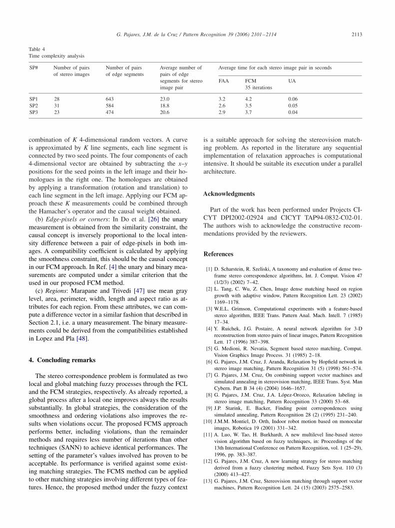
3.4. Time complexity analysis

Table 4 summarizes the results in terms of time complex-ity for the full process (FAA, FCM and UA). The analysisis carried out for each group of stereo pairs, first column;the number of stereo images for each group is displayed inthe second column; the number of pairs of features (edge-segments) for each group is shown in the third column; theaverage number of pairs of edge segments for each pair ofstereo images is displayed in the fourth column; the aver-age execution time in seconds for each stereo image pair isshown in fifth, sixth and seventh columns for FAA, FCMand UA processes, respectively. The time for FCM is com-puted after the execution of 35 iterations according to theresults in Table 2.

The execution times have been obtained from a code im-plemented in MATLAB and then compiled under MicrosoftVisual C++ and executed on a Pentium IV at 2.5 GHz with1 GB RAM. From results in Table 4 we can conclude thatthe time is directly proportional to the number of pairs ofedge segments processed. We also can see that an importanttime is spent during the FAA process. Moreover, as alreadyreported in the literature relaxation approaches are compu-tational intensive. For real time applications or critical timescheduling, it is suggested the implementation under paral-lel architectures. So, during the FAA process each image ofthe stereo pair can be processed in different processors andthen the FCM iterative process could be separated into dif-ferent clusters of nodes and those clusters assigned to dif-ferent processors. Also, we can point out that the execution

times for other global matching strategies analyzed fall insimilar ranges.

3.5. Extensions

The FCM relaxation scheme can be applied to differentstereovision matching schemes involving different features,such as edge-pixels, corner-pixels, curved segments or re-gions, by modifying or fitting the unary and binary relations.This implies that the unique requirement is the appropriatedmapping of the local stereovision matching constraints forunary and the global stereovision matching constraints forbinary. Taking into account Eq. (5) , the concept values Cij

and the causal weights wij are obtained from the unary andbinary measurements, respectively. If several unary or binarymeasurements are obtained, we can apply the Hamacher’sunion operator as in Eq. (10). In our approach this operatoris used only for combining the three binary measures used.The relaxation process is applied as in this approach. Someexamples for computing the unary and binary measurementsare given below:

(a) Curve-segments: In Nasrabadi [22] curved-segmentsare extracted by joining zero-crossings according to the pro-cedure described in Ballard [46]. Each curved-segment is la-beled and its centroid computed. The unary is a measure oflocal similarity computed as a ratio between the Hough ac-cumulator value obtained from the comparison between theleft and right R-tables of the involved curved-segment. Thebinary relation is a compatibility measure computed from thedistances between the four centroids involved. The conceptvalues and causal weights required by our FCM approachcan be directly obtained from the corresponding measure-ments. Shan and Zhang [25] compute the unary measure-ment by selecting seed points on both the left and the rightcurves, the right seed points are obtained by intersecting theepipolar lines of the left seed points with the curve in theright image; for each seed point on the left curve and itscorresponding point in the right curve a correlation scorebetween their neighborhoods is computed. This correlationscore should be the concept value in our FCM approach. Thebinary measurement in Ref. [25] is obtained as a weighted


Tabl

e3

Thr

esho

lds

and

setti

ngs

used

inth

ispa

per

Mod

ule

Des

crip

tion

Val

ue(s

)R

elev

ance

Com

men

ts

FAA

Gra

dien

ted

gepi

xel

join

ing

(mag

nitu

de,

dire

ctio

n)±2

0%,±4

5◦L

owC

ould

rang

ein

±30%

and

±90◦

Gra

dien

ted

gese

gmen

tdi

ffer

ence

for

mat

chin

g(m

agni

tude

,di

rect

ion)

15,

25◦

Med

ium

Cou

ldra

nge

betw

een

[0,3

0]an

d[0

◦ ,45

◦ ],

resp

ectiv

ely.

Ifth

eva

lues

incr

ease

,th

enu

mbe

rof

pair

sto

bem

atch

edin

crea

ses

Ove

rlap

rate

0.5

Med

ium

Ran

ges

in[0

,1].

Hig

hva

lues

decr

ease

sth

enu

mbe

rof

pair

san

ddo

not

allo

wbr

oken

edge

segm

ents

m,�

and

K(S

ectio

n2.

2,tr

aini

ngpr

oces

s)4.

2,0.

01,

10L

owm

coul

dra

nge

in[3

.5,5

.2];

�an

dK

coul

dre

ach

0.1

and

30,r

espe

ctiv

ely

FCM

Dis

pari

tylim

it,m

axd

15H

igh

Dep

ends

onth

eba

selin

ein

the

optic

ssy

stem

geom

etry

.In

our

syst

emth

eba

selin

eis

20cm

.C

ould

rang

ein

[5,2

5]D

eter

min

esth

ene

ighb

orho

odC

ompa

tibili

tyco

effic

ient

slop

e,�

inE

q.(6

)6

Hig

hD

eriv

edfr

omR

efs.

[41,

42].

Cou

ldra

nge

in[2

,15]

Con

stra

int

viol

atio

ns,U

0,

H0.

85M

ediu

mH

igh

valu

esar

ere

quir

edfo

rca

usal

conc

epts

ofm

atch

eded

gese

gmen

tsPa

ram

eter

inth

eH

amac

her’

sop

erat

or,�

1L

owC

ompe

nsat

ion

para

met

erbe

twee

nop

timis

tican

dpe

ssim

istic

boun

dsfo

rag

greg

atio

nfu

zzy

sets

.��

−1

Sigm

oid

func

tion

para

met

er,�

3.0

Low

Wel

lte

sted

inth

ene

ural

netw

ork

cont

ext

Max

imum

num

ber

ofite

ratio

ns,t m

ax

100

Hig

hM

ust

besu

ffici

ent

toen

sure

the

conv

erge

nce,

grea

ter

than

35U

AD

isam

bigu

atio

n,U

10.

5L

owT

his

isth

ein

term

edia

test

ate

valu

e.It

rang

esin

[−1,

1]D

iffe

renc

ein

segm

ents

orie

ntat

ions

,U

2±1

0◦L

owT

hesy

stem

geom

etry

limits

such

diff

eren

ce.

Itco

uld

reac

h±2

0◦


Table 4Time complexity analysis

SP# Number of pairs Number of pairs Average number of Average time for each stereo image pair in secondsof stereo images of edge segments pairs of edge

segments for stereo FAA FCM UAimage pair 35 iterations

SP1 28 643 23.0 3.2 4.2 0.06SP2 31 584 18.8 2.6 3.5 0.05SP3 23 474 20.6 2.9 3.7 0.04

combination of K 4-dimensional random vectors. A curveis approximated by K line segments, each line segment isconnected by two seed points. The four components of each4-dimensional vector are obtained by subtracting the x–ypositions for the seed points in the left image and their ho-mologues in the right one. The homologues are obtainedby applying a transformation (rotation and translation) toeach line segment in the left image. Applying our FCM ap-proach these K measurements could be combined throughthe Hamacher’s operator and the causal weight obtained.

(b) Edge-pixels or corners: In Do et al. [26] the unarymeasurement is obtained from the similarity constraint, thecausal concept is inversely proportional to the local inten-sity difference between a pair of edge-pixels in both im-ages. A compatibility coefficient is calculated by applyingthe smoothness constraint, this should be the causal conceptin our FCM approach. In Ref. [4] the unary and binary mea-surements are computed under a similar criterion that theused in our proposed FCM method.

(c) Regions: Marapane and Trivedi [47] use mean graylevel, area, perimeter, width, length and aspect ratio as at-tributes for each region. From these attributes, we can com-pute a difference vector in a similar fashion that described inSection 2.1, i.e. a unary measurement. The binary measure-ments could be derived from the compatibilities establishedin Lopez and Pla [48].

4. Concluding remarks

The stereo correspondence problem is formulated as twolocal and global matching fuzzy processes through the FCLand the FCM strategies, respectively. As already reported, aglobal process after a local one improves always the resultssubstantially. In global strategies, the consideration of thesmoothness and ordering violations also improves the re-sults when violations occur. The proposed FCMS approachperforms better, including violations, than the remaindermethods and requires less number of iterations than othertechniques (SANN) to achieve identical performances. Thesetting of the parameter’s values involved has proven to beacceptable. Its performance is verified against some exist-ing matching strategies. The FCMS method can be appliedto other matching strategies involving different types of fea-tures. Hence, the proposed method under the fuzzy context

is a suitable approach for solving the stereovision match-ing problem. As reported in the literature any sequentialimplementation of relaxation approaches is computationalintensive. It should be suitable its execution under a parallelarchitecture.

Acknowledgments

Part of the work has been performed under Projects CI-CYT DPI2002-02924 and CICYT TAP94-0832-C02-01.The authors wish to acknowledge the constructive recom-mendations provided by the reviewers.

References

[1] D. Scharstein, R. Szeliski, A taxonomy and evaluation of dense two-frame stereo correspondence algorithms, Int. J. Comput. Vision 47(1/2/3) (2002) 7–42.

[2] L. Tang, C. Wu, Z. Chen, Image dense matching based on regiongrowth with adaptive window, Pattern Recognition Lett. 23 (2002)1169–1178.

[3] W.E.L. Grimson, Computational experiments with a feature-basedstereo algorithm, IEEE Trans. Pattern Anal. Mach. Intell. 7 (1985)17–34.

[4] Y. Ruichek, J.G. Postaire, A neural network algorithm for 3-Dreconstruction from stereo pairs of linear images, Pattern RecognitionLett. 17 (1996) 387–398.

[5] G. Medioni, R. Nevatia, Segment based stereo matching, Comput.Vision Graphics Image Process. 31 (1985) 2–18.

[6] G. Pajares, J.M. Cruz, J. Aranda, Relaxation by Hopfield network instereo image matching, Pattern Recognition 31 (5) (1998) 561–574.

[7] G. Pajares, J.M. Cruz, On combining support vector machines andsimulated annealing in stereovision matching, IEEE Trans. Syst. ManCybern. Part B 34 (4) (2004) 1646–1657.

[8] G. Pajares, J.M. Cruz, J.A. López-Orozco, Relaxation labeling instereo image matching, Pattern Recognition 33 (2000) 53–68.

[9] J.P. Starink, E. Backer, Finding point correspondences usingsimulated annealing, Pattern Recognition 28 (2) (1995) 231–240.

[10] J.M.M. Montiel, D. Orth, Indoor robot motion based on monocularimages, Robotica 19 (2001) 331–342.

[11] A. Luo, W. Tao, H. Burkhardt, A new multilevel line-based stereovision algorithm based on fuzzy techniques, in: Proceedings of the13th International Conference on Pattern Recognition, vol. 1 (25–29),1996, pp. 383–387.

[12] G. Pajares, J.M. Cruz, A new learning strategy for stereo matchingderived from a fuzzy clustering method, Fuzzy Sets Syst. 110 (3)(2000) 413–427.

[13] G. Pajares, J.M. Cruz, Stereovision matching through support vectormachines, Pattern Recognition Lett. 24 (15) (2003) 2575–2583.


[14] D.H. Kim, R.H. Park, Analysis of quantization error in line-basedstereo matching, Pattern Recognition 8 (1994) 913–924.

[15] D.M. Wuescher, K.L. Boyer, Robust contour decomposition usinga constraint curvature criterion, IEEE Trans. Pattern Anal. Mach.Intell. 13 (1) (1991) 41–51.

[16] G. Pajares, J.M. Cruz, Stereo matching using Hebbian learning, IEEETrans. Syst. Man Cybern. Part B: Cybern. 29 (4) (1999) 553–559.

[17] G. Pajares, J.M. Cruz, The non-parametric Parzen’s window instereovision matching, IEEE Trans. Syst. Man Cybern. Part B:Cybern. 32 (2) (2002) 225–230.

[18] R. Hummel, S. Zucker, On the foundations of relaxation labellingprocesses, IEEE Trans. Pattern Anal. Mach. Intell. 5 (1983)267–287.

[19] D. Marr, T. Poggio, A computational theory of human stereovision,Proc. R. Soc. London B 207 (1979) 301–328.

[20] K.P. Han, T.M. Bae, Y.H. Ha, Hybrid stereo matching with anew relaxation scheme of preserving disparity discontinuity, PatternRecognition 33 (2000) 767–785.

[21] A. Rosenfeld, R. Hummel, S. Zucker, Scene labelling by relaxationoperation, IEEE Trans. Syst. Man Cybern. 6 (1976) 420–453.

[22] N.M. Nasrabadi, A stereo vision technique using curve-segments andrelaxation matching, IEEE Trans. Pattern Anal. Mach. Intell. 14 (5)(1992) 566–572.

[23] K.E. Price, Relaxation matching techniques—a comparison, IEEETrans. Pattern Anal. Mach. Intell. 7 (5) (1985) 617–623.

[24] W.J. Christmas, J. Kittler, M. Petrou, Structural matching in computervision using probabilistic relaxation, IEEE Trans. Pattern Anal. Mach.Intell. 17 (8) (1995) 749–764.

[25] Y. Shan, Z. Zhang, New measurements and corner-guidance for curvematching with probabilistic relaxation, Int. J. Comput. Vision 46 (2)(2002) 157–171.

[26] K.H. Do, Y.S. Kim, T.U. Uam, Y.H. Ha, Iterative relaxational stereomatching based on adaptive support between disparities, PatternRecognition 31 (8) (1998) 1049–1059.

[27] K.P. Han, T.M. Bae, Y.H. Ha, Hybrid stereo matching with anew relaxation scheme of preserving disparity discontinuity, PatternRecognition 33 (2000) 767–785.

[28] M.S. Mousavi, R.J. Schalkoff, ANN implementation of stereo visionusing a multi-layer feedback architecture, IEEE Trans. Syst. ManCybern. 24 (8) (1994) 1220–1238.

[29] N.M. Nasrabadi, C.Y. Choo, Hopfield network for stereovisioncorrespondence, IEEE Trans. Neural Networks 3 (1992) 123–135.

[30] Q. Cheng, Z.T. Fang, The stability problem for fuzzy bidirectionalassociative memories, Fuzzy Sets Syst. 132 (2002) 83–90.

[31] A.S. Martchenko, I.L. Ermolov, P.P. Groumpos, J.V. Poduraev, C.D.Stylios, Investigating stability analysis issues for fuzzy cognitivemaps, 11th Mediterranean Conference on Control and Automation,2003, pp. 1–6 (CD-ROM).

[32] A. Huertas, G. Medioni, Detection of intensity changes with subpixelaccuracy using Laplacian–Gaussian masks, IEEE Trans. Pattern Anal.Mach. Intell. 8 (5) (1986) 651–664.

[33] J.G. Leu, H.L. Yau, Detecting the dislocations in metal crystals frommicroscopic images, Pattern Recognition 24 (1991) 41–56.

[34] M.S. Lew, T.S. Huang, K. Wong, Learning and feature selectionin stereo matching, IEEE Trans. Pattern Anal. Mach. Intell. 16 (9)(1994) 869–881.

[35] E.P. Krotkov, Active Computer Vision by Cooperative Focus andStereo, Springer, New York, 1989.

[36] S. Tanaka, A.C. Kak, A rule-based approach to binocular stereopsis,in: R.C. Jain, A.K. Jain (Eds.), Analysis and Interpretation of RangeImages, Springer, Berlin, 1990, pp. 33–139.

[37] R. Nevatia, K.R. Babu, Linear feature extraction and description,Comput. Vision Graphics Image Process. 13 (1980) 257–269.

[38] B. Kosko, Neural Networks and Fuzzy Systems: A DynamicalSystems Approach to Machine Intelligence, Prentice-Hall, EnglewoodCliffs, NJ, 1992.

[39] B. Kosko, Fuzzy cognitive maps, Int. J. Man Mach. Stud. 24 (1986)65–75.

[40] S. Haykin, Neural Networks: A Comprehensive Foundation,Macmillan, New York, 1994.

[41] S.T. Barnard, Stochastic stereo matching over scale, Int. J. Comput.Vision 3 (1) (1989) 17–32.

[42] S. Hattori, A. Okamoto, H. Hasegawa, Stereo matching by simulatedannealing incorporating a diffusion equation, Proceedings of theASPRS 1998 Annual Conference, 1998, pp. 1030–1041.

[43] J.R. Hilera, V.J. Martínez, Redes Neuronales Artificiales, RA-MA,1995.

[44] H.J. Zimmermann, Fuzzy Set Theory and its Applications, KluwerAcademic Publishers, Dordrecht, 1991.

[45] T. Poggio, V. Torre, C. Koch, Computational vision and regularizationtheory, Nature 317 (1985) 314–319.

[46] D.H. Ballard, Generalizing the Hough transform to detect arbitraryshapes, Pattern Recognition 13 (2) (1981) 111–122.

[47] S.B. Marapane, M.M. Trivedi, Region-based stereo analysis forrobotic applications, IEEE Trans. Syst. Man Cybern. 19 (6) (1989)1447–1464.

[48] A. Lopez, F. Pla, Dealing with segmentation errors in region-basedstereo matching, Pattern Recognition 33 (2000) 1325–1338.

Fuzzy Cognitive Maps for stereovision matching

Documents

Transcript of Fuzzy Cognitive Maps for stereovision matching