Improving a symbolic parser through partially supervised ...
Upload
khangminh22Category
view
0download
0
COMPRESSION, GENERATION, AND INFERENCE VIA SUPERVISED LEARNING
A DISSERTATIONSUBMITTED TO THE DEPARTMENT OF COMPUTER SCIENCE
AND THE COMMITTEE ON GRADUATE STUDIESOF STANFORD UNIVERSITY
IN PARTIAL FULFILLMENT OF THE REQUIREMENTSFOR THE DEGREE OF
DOCTOR OF PHILOSOPHY
Jiaming SongDecember 2021

Abstract
Articial intelligence and machine learning methods have seen tremendous advances in the pastdecade, thanks to deep neural networks. Supervised learning methods enables neural networks toeectively approximate low-level functions of human intelligence, such as identifying an objectwithin an image. However, many complex functions of human intelligence are dicult to solve withsupervised learning directly: humans can build concise representations of the world (compression),generate works of art based on creative imaginations (generation), and infer how others will actfrom personal experiences (inference).
In this dissertation, we focus on machine learning approaches that reduce these complexfunctions of human intelligence into simpler ones that can be readily solved with supervisedlearning and thus enabling us to leverage the developments in deep learning. This dissertationcomprises of three parts, namely compression, generation, and inference.
The rst part discusses how we can apply supervised learning to unsupervised representationlearning. We develop algorithms that can learn informative representations from large unlabeleddatasets while protecting certain sensitive attributes. The second part extends these ideas tolearning high-dimensional probabilistic models of unlabeled data. Combined with the insightsfrom the rst part, we introduce a generative model suitable for conditional generation underlimited supervision. In the third and nal part, we present two applications of supervised learningin probabilistic inference methods: (a) optimizing for ecient Bayesian inference algorithms and(b) inferring the agents’ intent under complex, multi-agent environments. These contributionsenable machines to overcome existing limitations of supervised learning in real-world compression,generation, and inference problems.
iv

Acknowledgments
First and foremost, I would like to thank my Ph.D. advisor, Stefano Ermon. I had a fantastic Ph.D.experience with Stefano in the past four and a half years, which would not have been possiblewithout Stefano’s patient advice over my research and the liberty he gave me to pursue my personalresearch interests. Stefano has an amazing depth and breadth of knowledge about various elds inmachine learning and can answer my questions whenever I need to. I will never forget his adviceon type checks and rigorous theory statements during many hours of paper writing, and I oftenfeel that he treats the rigor in my papers and talks more seriously than I do; I am both sorry andthankful for these moments. Outside of core machine learning, Stefano also has keen insights aboutvaluable scientic domains to work on, such as computational sustainability, instead of simplypursuing what are “hot”. I hope that I will learn these essential qualities of an advisor in my futureacademic career and that our collaborations will remain fruitful.
My journey at Stanford would not be complete without the company I enjoyed with peers,especially at the Stanford AI lab. Aditya Grover’s research has shaped my own a lot, and hewas of tremendous help during every important step of my Ph.D. Shengjia Zhao, my roommatefor four years, continues to be a huge inspiration for life and research. Jonathan Kuck and RuiShu were amazing lab mates with a lot of fun. I learned a lot from Yang Song, and we had ablast sailing, golng, and playing computer games. Kuno was a great gym buddy (and instructor)before covid, and my dissertation talk would not be the same without him. Lantao Yu is a veryreliable collaborator, and we had amazing times skiing and playing board games. Kristy Choi wasan incredible host at her home parties and my Ph.D. “farewell” dinner. Tri Dao was extremelyhelpful during my quarter as course assistant and an inspirational gym buddy. Chenlin Meng hasunparalleled work ethic and many projects were made possible by her. I learned a lot from moresenior lab mates: Volodymyr Kuleshov, Russell Stewart, Jonathan Ho, and Burak Ukzent, and hopeto learn even more from newer ones: Chris Cundy, Andy Shih, Willie Neiswanger, Charlie Marx,and Gengchen Mai. I also miss hanging out with the many friends at StatsML group and InfoLab,
v

and others from places such as UC Berkeley, MIT, Tsinghua and Toronto.I have also had the privilege of the guidance of various amazing mentors over the years. Jun
Zhu gave me my rst experiences in machine learning research when I was an undergraduate atTsinghua University, and I extended this experience with Wenwu Zhu and Peng Cui. LawrenceCarin and many of his students, including Zhe Gan, Chunyuan Li, Changyou Chen, Yizhe Zhang,Yunchen Pu, were accomodating during my stay at Duke University and are one of the reasons why Ipursued a Ph.D. after undergrad. Chelsea Finn, Dorsa Sadigh, Emma Brunskill, Mykel Kochenderfer,Peter Bailis, Jiajun Wu, and Tengyu Ma were generous with their insightful feedback and timeduring rotations, quals, oral exams and the dissertation. John Schulman, Yan Duan, Tengyu Ma,Yann Dauphin and Michael Auli broadened my research perspectives in summer internships atOpenAI and Facebook. I have also enjoyed discussions with collaborators who helped me withinteresting ideas in research: Abhishek Sinha, Ali Malik, Divyansh Garg, Hongyu Ren, LaëtitiaShao, Nate Gruver, Samarth Sinha, Yilun Xu, Yuhuai Wu, Yunzhu Li, and Yusuke Tashiro.
This dissertation would not have been possible with my many other co-authors: Aidan Perreault,Akshat Jindal, Alekh Agarwal, Ali Malik, Animesh Garg, Arianna Yuan, Ashish Kapoor, AshishSabharwal, Ayush Kumar, Danny Nemer, Eric J. Horvitz, Hao Tang, Harlan Seymour, Hongxia Jin,Huazhong Yang, Huimin Ma, Jiayu Chen, Jun-Yan Zhu, Kenneth Tran, Noah Goodman, RachelLuo, Silvio Savarese, Shuvam Chakraborty, Yanan Sui, Yihong Gu, Yu Wang, Yuanfan Xu, YuanxinZhang, and Yutong He. I thank them for their contributions.
During my job search, I was extremely fortunate to have received encouraging guidance fromresearchers in various institutions. In addition to those mentioned above, I especially thank DavidMcAllester for supporting my application, Je Ullman and Keith Weinstein for your honest andhelpful opinion on my job talk, Yang Gao, Yi Wu, and Huazhe Xu for sound advice for the variousstatements, and Danfei Xu and Wei Hu for sharing ups and downs during the interview process. Ialso appreciate the support of all funding agencies, including the Qualcomm Innovation Fellowshipand research grants from NSF, the Toyota Research Institute, the Future of Life Institute, Siemens,Sony, and Lam Research.
I would also like to thank many other friends who were a crucial part of the journey. I havehad many fond memories having fun, meeting and travelling around the world with you, and I willcherish these moments forever.
Finally, I would like to thank my family for their love and support, especially my parents andmy ancé Chenchen. I am forever indebted to you.
vi

Contents
Abstract iv
Acknowledgments v
1 Introduction 1
1.1 Overview . . . . . . . . . . . . . . . . . . . . . . . . . . . . . . . . . . . . . . . . . 21.1.1 Compression via Supervised Learning . . . . . . . . . . . . . . . . . . . . 21.1.2 Generation via Supervised Learning . . . . . . . . . . . . . . . . . . . . . 41.1.3 Inference via Supervised Learning . . . . . . . . . . . . . . . . . . . . . . 6
1.2 Dissertation Structure . . . . . . . . . . . . . . . . . . . . . . . . . . . . . . . . . . 8
2 Background 10
2.1 Comparing and Optimizing Distributions . . . . . . . . . . . . . . . . . . . . . . . 102.1.1 Compression . . . . . . . . . . . . . . . . . . . . . . . . . . . . . . . . . . 122.1.2 Generation . . . . . . . . . . . . . . . . . . . . . . . . . . . . . . . . . . . 122.1.3 Inference . . . . . . . . . . . . . . . . . . . . . . . . . . . . . . . . . . . . 14
2.2 Variational Methods for Comparing Distributions . . . . . . . . . . . . . . . . . . 152.2.1 Lower bounds of f -divergences . . . . . . . . . . . . . . . . . . . . . . . . 162.2.2 Upper bounds of f -divergences . . . . . . . . . . . . . . . . . . . . . . . . 17
I Compression via Supervised Learning 19
3 Compression via Mutual Information 20
3.1 Introduction . . . . . . . . . . . . . . . . . . . . . . . . . . . . . . . . . . . . . . . 213.2 Background and Related Work . . . . . . . . . . . . . . . . . . . . . . . . . . . . . 21
vii

3.2.1 Variational Mutual Inforamtion Estimation . . . . . . . . . . . . . . . . . 223.3 Variational mutual information estimation as optimization over density ratios . . 24
3.3.1 A summary of existing variational methods . . . . . . . . . . . . . . . . . 243.3.2 Generative and discriminative approaches to MI estimation . . . . . . . . 25
3.4 Limitations of existing variational estimators . . . . . . . . . . . . . . . . . . . . . 263.4.1 Good discriminative estimators require exponentially large batches . . . . 263.4.2 Self-consistency issues for mutual information estimators . . . . . . . . . 27
3.5 Mutual information estimation via clipped density ratios . . . . . . . . . . . . . . 283.6 Experiments . . . . . . . . . . . . . . . . . . . . . . . . . . . . . . . . . . . . . . . 29
3.6.1 Benchmarking on multivariate Gaussians . . . . . . . . . . . . . . . . . . 293.6.2 Self-consistency tests on Images . . . . . . . . . . . . . . . . . . . . . . . . 31
3.7 Discussion . . . . . . . . . . . . . . . . . . . . . . . . . . . . . . . . . . . . . . . . 33
4 Representation Learning via Classication 34
4.1 Introduction . . . . . . . . . . . . . . . . . . . . . . . . . . . . . . . . . . . . . . . 354.2 Contrastive Predictive Coding and Mutual Information . . . . . . . . . . . . . . . 36
4.2.1 Re-weighted Contrastive Predictive Coding . . . . . . . . . . . . . . . . . 374.3 Multi-label Contrastive Predictive Coding . . . . . . . . . . . . . . . . . . . . . . . 38
4.3.1 Re-weighted Multi-label Contrastive Predictive Coding . . . . . . . . . . . 394.4 Related Work . . . . . . . . . . . . . . . . . . . . . . . . . . . . . . . . . . . . . . . 414.5 Experiments . . . . . . . . . . . . . . . . . . . . . . . . . . . . . . . . . . . . . . . 43
4.5.1 Mutual Information Estimation . . . . . . . . . . . . . . . . . . . . . . . . 434.5.2 Knowledge Distillation . . . . . . . . . . . . . . . . . . . . . . . . . . . . . 444.5.3 Representation Learning . . . . . . . . . . . . . . . . . . . . . . . . . . . . 46
4.6 Discussion . . . . . . . . . . . . . . . . . . . . . . . . . . . . . . . . . . . . . . . . 47
5 Fair Representation Learning via Regression 49
5.1 Introduction . . . . . . . . . . . . . . . . . . . . . . . . . . . . . . . . . . . . . . . 505.2 An Information-Theoretic Objective for Controllable Fair Representations . . . . 51
5.2.1 Tractable Lower Bound for Iq(x; z|u) . . . . . . . . . . . . . . . . . . . . 535.2.2 Tractable Upper Bound for Iq(z;u) . . . . . . . . . . . . . . . . . . . . . . 535.2.3 A Tighter Upper Bound to Iq(z,u) via Adversarial Training . . . . . . . . 535.2.4 A practical objective for controllable fair representations . . . . . . . . . . 55
5.3 A Unifying Framework for Related Work . . . . . . . . . . . . . . . . . . . . . . . 56
viii

5.4 Dual Optimization for Controllable Fair Representations . . . . . . . . . . . . . . 585.5 Experiments . . . . . . . . . . . . . . . . . . . . . . . . . . . . . . . . . . . . . . . 59
5.5.1 Experimental Setup . . . . . . . . . . . . . . . . . . . . . . . . . . . . . . . 595.5.2 Mutual Information, Prediction Accuracy, and Fairness . . . . . . . . . . . 605.5.3 Controlling Representation Fairness with L-MIFR . . . . . . . . . . . . . . 635.5.4 Improving Representation Expressiveness with L-MIFR . . . . . . . . . . . 635.5.5 Ablation Studies . . . . . . . . . . . . . . . . . . . . . . . . . . . . . . . . 655.5.6 Fair Representations under Multiple Notions . . . . . . . . . . . . . . . . . 65
5.6 Discussion . . . . . . . . . . . . . . . . . . . . . . . . . . . . . . . . . . . . . . . . 66
II Generation via Supervised Learning 67
6 Generation with Reweighted Objectives 68
6.1 Introduction . . . . . . . . . . . . . . . . . . . . . . . . . . . . . . . . . . . . . . . 686.2 Preliminaries . . . . . . . . . . . . . . . . . . . . . . . . . . . . . . . . . . . . . . . 706.3 A Generalization of f -GANs and WGANs . . . . . . . . . . . . . . . . . . . . . . . 71
6.3.1 Recovering the f -GAN Critic Objective . . . . . . . . . . . . . . . . . . . 726.3.2 Recovering the WGAN Critic Objective . . . . . . . . . . . . . . . . . . . 736.3.3 Extensions to Alternative Constraints . . . . . . . . . . . . . . . . . . . . 73
6.4 Practical f -Wasserstein GANs . . . . . . . . . . . . . . . . . . . . . . . . . . . . . 756.4.1 KL-Wasserstein GANs . . . . . . . . . . . . . . . . . . . . . . . . . . . . . 756.4.2 Implementation Details . . . . . . . . . . . . . . . . . . . . . . . . . . . . 76
6.5 Related Work . . . . . . . . . . . . . . . . . . . . . . . . . . . . . . . . . . . . . . . 776.5.1 f -divergences, IPMs and GANs . . . . . . . . . . . . . . . . . . . . . . . . 776.5.2 Reweighting of Generated Samples . . . . . . . . . . . . . . . . . . . . . . 78
6.6 Experiments . . . . . . . . . . . . . . . . . . . . . . . . . . . . . . . . . . . . . . . 786.6.1 Synthetic and UCI Benchmark Datasets . . . . . . . . . . . . . . . . . . . 786.6.2 Image Generation . . . . . . . . . . . . . . . . . . . . . . . . . . . . . . . . 82
6.7 Discussion . . . . . . . . . . . . . . . . . . . . . . . . . . . . . . . . . . . . . . . . 82
7 Generation with Negative Data Augmentation 84
7.1 Introduction . . . . . . . . . . . . . . . . . . . . . . . . . . . . . . . . . . . . . . . 857.2 Negative Data Augmentation . . . . . . . . . . . . . . . . . . . . . . . . . . . . . . 86
ix

7.3 NDA for Generative Adversarial Networks . . . . . . . . . . . . . . . . . . . . . . 887.4 NDA for Constrastive Representation Learning . . . . . . . . . . . . . . . . . . . . 907.5 NDA-GAN Experiments . . . . . . . . . . . . . . . . . . . . . . . . . . . . . . . . . 917.6 Representation Learning using Contrastive Loss and NDA . . . . . . . . . . . . . 957.7 Related work . . . . . . . . . . . . . . . . . . . . . . . . . . . . . . . . . . . . . . . 967.8 Discussion . . . . . . . . . . . . . . . . . . . . . . . . . . . . . . . . . . . . . . . . 97
8 Generation with Learned Conditions 98
8.1 Introduction . . . . . . . . . . . . . . . . . . . . . . . . . . . . . . . . . . . . . . . 998.2 Background . . . . . . . . . . . . . . . . . . . . . . . . . . . . . . . . . . . . . . . 1008.3 Problem Statement . . . . . . . . . . . . . . . . . . . . . . . . . . . . . . . . . . . 1018.4 Denoising Diusion Implicit Models . . . . . . . . . . . . . . . . . . . . . . . . . . 101
8.4.1 Training diusion models . . . . . . . . . . . . . . . . . . . . . . . . . . . 1038.4.2 DDIM sampling procedure . . . . . . . . . . . . . . . . . . . . . . . . . . . 104
8.5 Diusion-Decoding Generative Models with Contrastive Learning . . . . . . . . . 1058.5.1 Relationship to maximum likelihood . . . . . . . . . . . . . . . . . . . . . 1068.5.2 D2C models address latent posterior mismatch in VAEs . . . . . . . . . . 107
8.6 Few-shot Conditional Generation with D2C . . . . . . . . . . . . . . . . . . . . . 1088.7 Related Work . . . . . . . . . . . . . . . . . . . . . . . . . . . . . . . . . . . . . . . 1118.8 Experiments . . . . . . . . . . . . . . . . . . . . . . . . . . . . . . . . . . . . . . . 112
8.8.1 Unconditional generation . . . . . . . . . . . . . . . . . . . . . . . . . . . 1128.8.2 Few-shot conditional generation from examples . . . . . . . . . . . . . . . 1148.8.3 Few-shot conditional generation from manipulation constraints . . . . . . 115
8.9 Discussions . . . . . . . . . . . . . . . . . . . . . . . . . . . . . . . . . . . . . . . . 115
III Inference via Supervised Learning 118
9 Learning Kernels for Markov Chain Monte Carlo 119
9.1 Introduction . . . . . . . . . . . . . . . . . . . . . . . . . . . . . . . . . . . . . . . 1209.2 Notations and Problem Setup . . . . . . . . . . . . . . . . . . . . . . . . . . . . . . 1219.3 Adversarial Training for Markov Chains . . . . . . . . . . . . . . . . . . . . . . . 122
9.3.1 Example: Generative Model for Images . . . . . . . . . . . . . . . . . . . . 1239.4 Adversarial Training for Markov Chain Monte Carlo . . . . . . . . . . . . . . . . 125
x

9.4.1 Exact Sampling Through MCMC . . . . . . . . . . . . . . . . . . . . . . . 1259.4.2 Hamiltonian Monte Carlo and Volume Preserving Flow . . . . . . . . . . 1269.4.3 A NICE Proposal . . . . . . . . . . . . . . . . . . . . . . . . . . . . . . . . 1279.4.4 Training A NICE Proposal . . . . . . . . . . . . . . . . . . . . . . . . . . . 1289.4.5 Bootstrap . . . . . . . . . . . . . . . . . . . . . . . . . . . . . . . . . . . . 1299.4.6 Reducing Autocorrelation by Pairwise Discriminator . . . . . . . . . . . . 129
9.5 Experiments . . . . . . . . . . . . . . . . . . . . . . . . . . . . . . . . . . . . . . . 1309.6 Discussion . . . . . . . . . . . . . . . . . . . . . . . . . . . . . . . . . . . . . . . . 133
10 Learning Intentions for Multi-agent Interactions 134
10.1 Introduction . . . . . . . . . . . . . . . . . . . . . . . . . . . . . . . . . . . . . . . 13510.2 Preliminaries . . . . . . . . . . . . . . . . . . . . . . . . . . . . . . . . . . . . . . . 136
10.2.1 Markov games . . . . . . . . . . . . . . . . . . . . . . . . . . . . . . . . . 13610.2.2 Reinforcement learning and Nash equilibrium . . . . . . . . . . . . . . . . 13710.2.3 Inverse reinforcement learning . . . . . . . . . . . . . . . . . . . . . . . . 13910.2.4 Solution Concepts for Markov Games . . . . . . . . . . . . . . . . . . . . 13910.2.5 Imitation by matching occupancy measures . . . . . . . . . . . . . . . . . 14010.2.6 Adversarial Inverse Reinforcement Learning . . . . . . . . . . . . . . . . . 140
10.3 Generalizing Imitation Learning to Markov games . . . . . . . . . . . . . . . . . . 14110.3.1 Equivalent constraints via temporal dierence learning . . . . . . . . . . . 14210.3.2 Multi-agent imitation learning . . . . . . . . . . . . . . . . . . . . . . . . 143
10.4 Practical multi-agent imitation learning . . . . . . . . . . . . . . . . . . . . . . . . 14510.4.1 Multi-agent generative adversarial imitation learning . . . . . . . . . . . . 14510.4.2 Multi-agent actor-critic with Kronecker factors . . . . . . . . . . . . . . . 147
10.5 Scaling up Multi-agent Inverse Reinforcement Learning . . . . . . . . . . . . . . . 14810.5.1 Scalable Modeling with Latent Variables . . . . . . . . . . . . . . . . . . . 14810.5.2 Multi-agent AIRL with Latent Variables . . . . . . . . . . . . . . . . . . . 149
10.6 Experiments . . . . . . . . . . . . . . . . . . . . . . . . . . . . . . . . . . . . . . . 15010.6.1 Particle environments . . . . . . . . . . . . . . . . . . . . . . . . . . . . . 15010.6.2 Cooperative control with MA-GAIL . . . . . . . . . . . . . . . . . . . . . . 15210.6.3 Transportation Environments . . . . . . . . . . . . . . . . . . . . . . . . . 153
10.7 Related work and discussion . . . . . . . . . . . . . . . . . . . . . . . . . . . . . . 158
xi

11 Conclusions 161
11.1 Summary of Contributions . . . . . . . . . . . . . . . . . . . . . . . . . . . . . . . 16111.2 Future Work . . . . . . . . . . . . . . . . . . . . . . . . . . . . . . . . . . . . . . . 162
A Proofs 164
B Additional Experimental Details & Results 193
C Code and Data 236
xii

List of Tables
3.1 Summarization of variational estimators of mutual information. . . . . . . . . . . 23
4.1 Knowledge distillation on CIFAR100. . . . . . . . . . . . . . . . . . . . . . . . . . 454.2 Knowledge distillation on CIFAR100 (cont’d). . . . . . . . . . . . . . . . . . . . . . 464.3 Top-1 accuracy of unsupervised representation learning. . . . . . . . . . . . . . . 474.4 ImageNet representation learning for 30 epochs. . . . . . . . . . . . . . . . . . . . 47
5.1 Summarizing the components in existing methods. . . . . . . . . . . . . . . . . . 575.2 Expressiveness and fairness trade-o. . . . . . . . . . . . . . . . . . . . . . . . . . 655.3 Learning one representation for multiple notions of fairness. . . . . . . . . . . . . 66
6.1 Evaluation of KL-WGAN on 2-d synthetic datasets. . . . . . . . . . . . . . . . . . 786.2 Evaluation of KL-WGAN on real-world datasets. . . . . . . . . . . . . . . . . . . . 806.3 Inception and FID scores for CIFAR10 image generation. . . . . . . . . . . . . . . 816.4 FID scores for CelebA image generation. . . . . . . . . . . . . . . . . . . . . . . . 82
7.1 FID scores over CIFAR-10 . . . . . . . . . . . . . . . . . . . . . . . . . . . . . . . . 937.2 Comparison of FID scores of dierent types of NDA . . . . . . . . . . . . . . . . . 937.3 FID scores for conditional image generation using dierent NDAs. . . . . . . . . . 937.4 Results on CityScapes . . . . . . . . . . . . . . . . . . . . . . . . . . . . . . . . . . 947.5 AUROC scores for dierent OOD datasets . . . . . . . . . . . . . . . . . . . . . . 947.6 NDA image recognition results. . . . . . . . . . . . . . . . . . . . . . . . . . . . . 957.7 NDA video recognition results. . . . . . . . . . . . . . . . . . . . . . . . . . . . . . 96
8.1 Several common paradigms for generative modeling. . . . . . . . . . . . . . . . . 1028.2 Quality of representations and generations with LVGMs. . . . . . . . . . . . . . . 1138.3 FID scores over dierent faces dataset with LVGMs. . . . . . . . . . . . . . . . . . 114
xiii

8.4 Sample quality as a function of diusion steps. . . . . . . . . . . . . . . . . . . . . 1148.5 Conditional generation from labels. . . . . . . . . . . . . . . . . . . . . . . . . . . 115
9.1 Performance of MCMC samplers as measured by Eective Sample Size (ESS). . . . 1319.2 ESS and ESS per second for Bayesian logistic regression tasks. . . . . . . . . . . . 133
10.1 Average agent rewards in competitive tasks . . . . . . . . . . . . . . . . . . . . . 15210.2 Results on the HighD dataset. . . . . . . . . . . . . . . . . . . . . . . . . . . . . . 15510.3 Results on the FAA dataset. . . . . . . . . . . . . . . . . . . . . . . . . . . . . . . . 155
B.1 Bias, Variance and MSE of the estimators under the joint critic. . . . . . . . . . . . 194B.2 Self-consistency experiments on other image transforms. . . . . . . . . . . . . . . 196B.3 Comparison between L-MIFR and LAFTR. . . . . . . . . . . . . . . . . . . . . . . 201B.4 Eect of λ on the FID score. . . . . . . . . . . . . . . . . . . . . . . . . . . . . . . 210B.5 Hyperparameters across dierent datasets . . . . . . . . . . . . . . . . . . . . . . 216B.6 CIFAR-10 image generation results. . . . . . . . . . . . . . . . . . . . . . . . . . . 218B.7 Performance in cooperative navigation. . . . . . . . . . . . . . . . . . . . . . . . . 233B.8 Performance in cooperative communication. . . . . . . . . . . . . . . . . . . . . . 233B.9 Performance in competitive tasks. . . . . . . . . . . . . . . . . . . . . . . . . . . . 234
xiv
List of Figures
1.1 Overview of the dissertation topic. . . . . . . . . . . . . . . . . . . . . . . . . . . . 21.2 Compression via Supervised Learning. . . . . . . . . . . . . . . . . . . . . . . . . 31.3 Supervised learning for generative models. . . . . . . . . . . . . . . . . . . . . . . 51.4 Overview of few-shot conditional generation. . . . . . . . . . . . . . . . . . . . . 61.5 Supervised learning for probabilistic inference. . . . . . . . . . . . . . . . . . . . . 61.6 Supervised learning for reward inference. . . . . . . . . . . . . . . . . . . . . . . . 7
2.1 Compression as optimizing a discrepancy. . . . . . . . . . . . . . . . . . . . . . . 132.2 Generation as optimizing a discrepancy. . . . . . . . . . . . . . . . . . . . . . . . . 132.3 Inference as optimizing a discrepancy. . . . . . . . . . . . . . . . . . . . . . . . . . 14
3.1 Evaluation over the SMILE estimator. . . . . . . . . . . . . . . . . . . . . . . . . . 303.2 Evaluation of various estimators. . . . . . . . . . . . . . . . . . . . . . . . . . . . . 313.3 Three settings in the self-consistency experiments. . . . . . . . . . . . . . . . . . 313.4 Evaluation of the rst setting. . . . . . . . . . . . . . . . . . . . . . . . . . . . . . 323.5 Evaluation of the second setting. . . . . . . . . . . . . . . . . . . . . . . . . . . . . 323.6 Evaluation of the third setting. . . . . . . . . . . . . . . . . . . . . . . . . . . . . . 33
4.1 MI estimates with CPC and ML-CPC under dierent α. . . . . . . . . . . . . . . . 414.2 Bias-variance trade-os for dierent negative samples. . . . . . . . . . . . . . . . 414.3 Mutual information estimation with ML-CPC. . . . . . . . . . . . . . . . . . . . . 434.4 Ablation studies for knowledge distillation. . . . . . . . . . . . . . . . . . . . . . . 45
5.1 Mutual information and fairness. . . . . . . . . . . . . . . . . . . . . . . . . . . . . 615.2 Constraints satisfaction with L-MIFR. . . . . . . . . . . . . . . . . . . . . . . . . . 625.3 Demographic parity with respect to constraints. . . . . . . . . . . . . . . . . . . . 64
xv

5.4 Expressiveness vs. the second constraint. . . . . . . . . . . . . . . . . . . . . . . . 64
6.1 High-level idea of f -WGAN. . . . . . . . . . . . . . . . . . . . . . . . . . . . . . . 746.2 KL-WGAN samples on 2d distributions. . . . . . . . . . . . . . . . . . . . . . . . . 796.3 Estimating density ratios with KL-WGAN. . . . . . . . . . . . . . . . . . . . . . . 796.4 Estimated divergence with KL-WGAN. . . . . . . . . . . . . . . . . . . . . . . . . 80
7.1 Negative Data Augmentation for GANs. . . . . . . . . . . . . . . . . . . . . . . . . 867.2 Negative augmentations produce out-of-distribution samples. . . . . . . . . . . . 877.3 Schematic overview of our NDA framework. . . . . . . . . . . . . . . . . . . . . . 887.4 Discriminator outputs for images. . . . . . . . . . . . . . . . . . . . . . . . . . . . 92
8.1 D2C demonstration. . . . . . . . . . . . . . . . . . . . . . . . . . . . . . . . . . . . 1008.2 Illustration of components of a D2 model. . . . . . . . . . . . . . . . . . . . . . . . 1068.3 Generated samples on CIFAR-10, fMoW, and FFHQ. . . . . . . . . . . . . . . . . . 1138.4 Conditional generation from manipulation constraints. . . . . . . . . . . . . . . . 1168.5 AMT evaluation over image manipulations. . . . . . . . . . . . . . . . . . . . . . . 116
9.1 Image samples from a Markov chain, on MNIST. . . . . . . . . . . . . . . . . . . . 1239.2 Tθ(yt+1|yt). . . . . . . . . . . . . . . . . . . . . . . . . . . . . . . . . . . . . . . . 1249.3 Image samples from a Markov chain, on CelebA. . . . . . . . . . . . . . . . . . . . 1249.4 Sampling process of A-NICE-MC. . . . . . . . . . . . . . . . . . . . . . . . . . . . 1289.5 Samples with and without a pairwise discriminator. . . . . . . . . . . . . . . . . . 1299.6 Densities of ring, mog2, mog6 and ring5. . . . . . . . . . . . . . . . . . . . . . . . 1319.7 Evaluation for A-NICE-MC. . . . . . . . . . . . . . . . . . . . . . . . . . . . . . . 1319.8 ESS with respect to the number of training iterations. . . . . . . . . . . . . . . . . 132
10.1 Dierent MAGAIL algorithms. . . . . . . . . . . . . . . . . . . . . . . . . . . . . . 14710.2 Average true reward from cooperative tasks . . . . . . . . . . . . . . . . . . . . . 15110.3 Rollouts on HighD dataset. . . . . . . . . . . . . . . . . . . . . . . . . . . . . . . . 15610.4 Rollouts on FAA dataset. . . . . . . . . . . . . . . . . . . . . . . . . . . . . . . . . 15710.5 Visualization of learned reward functions on HighD. . . . . . . . . . . . . . . . . . 15810.6 Visualization of learned reward functions on FAA. . . . . . . . . . . . . . . . . . . 159
A.1 Illustration of the construction in 2d. . . . . . . . . . . . . . . . . . . . . . . . . . 185
xvi

B.1 Bias / Variance / MSE of various estimators. . . . . . . . . . . . . . . . . . . . . . 195B.2 Additional benchmark results. . . . . . . . . . . . . . . . . . . . . . . . . . . . . . 195B.5 Toy Datasets used in Numerosity experiments. . . . . . . . . . . . . . . . . . . . . 207B.6 NDA for CLEVR dataset. . . . . . . . . . . . . . . . . . . . . . . . . . . . . . . . . 208B.7 Qualitative results on Cityscapes. . . . . . . . . . . . . . . . . . . . . . . . . . . . 209B.8 Histogram of D(clean) - D(corrupt) for 3 dierent corruptions. . . . . . . . . . . . 210B.9 Comparing the cosine distance of the representations. . . . . . . . . . . . . . . . . 210B.10 Amazon Mechanical Turk Demo . . . . . . . . . . . . . . . . . . . . . . . . . . . . 217B.11 Additional image samples for the FFHQ-256 dataset. . . . . . . . . . . . . . . . . . 219B.12 Image manipulation results for blond hair. . . . . . . . . . . . . . . . . . . . . . . 220B.13 Image manipulation results for red lipstick. . . . . . . . . . . . . . . . . . . . . . . 221B.14 Image manipulation results for beard. . . . . . . . . . . . . . . . . . . . . . . . . . 222B.15 Image manipulation results for gender. . . . . . . . . . . . . . . . . . . . . . . . . 223B.16 Conditional generation with D2C by learning from 100 labeled examples. . . . . . 224B.17 Conditional generation with DDIM by learning from 100 labeled examples. . . . . 224B.18 Conditional generation with D2C by learning from 100 labeled examples. . . . . . 225B.19 Conditional generation with DDIM by learning from 100 labeled examples. . . . . 225B.20 Generative process for the pairwise discriminator . . . . . . . . . . . . . . . . . . 227B.22 Sample complexity of multi-agent GAIL methods under cooperative tasks. . . . . 234
xvii

Chapter 1
Introduction
Deep function approximators, such as neural networks, are highly successful in supervised learning;given abundant labels that are directly provided by humans, neural networks can learn to maptraining data to the corresponding labels [HZRS16, SHM+16]. However, this learning paradigmdoes not suit complex algorithms that describe more sophisticated intelligent behaviors; theseinclude algorithms for eective compression of data, algorithms that synthesize novel data, andalgorithms that infer the reward models of human drivers. These algorithms are dicult to solvewith direct supervised learning, since the acquisition of “ground-truth” labels (e.g., compressedrepresentation of a data point, realism of a synthesized sample, reward of a driving trajectory)is either too expensive to acquire in mass quantities or challenging to dene even for domainexperts [Zho18, Bar89, Gha03, HTF09].
The goal of this dissertation is to build machines that learn these complex algorithms with min-imal direct supervision from humans. In particular, we discuss three key problems in unsupervisedmachine learning that are instances of the tasks1:
Compression (Figure 1.1a) : How can we extract compact and informative representations ofthe data that are useful for downstream goals (e.g., accuracy, privacy, fairness)? Theserepresentations can vastly reduce the need for labeled data in a new task.
Generation (Figure 1.1b) : How can we learn powerful generative models that capture complex,multi-modal distributions from data samples (e.g. images, videos, demonstrations)? Thesemodels can be used to manipulate existing data, evaluate test data, or synthesize new samples.
1We provide a detailed account of these tasks in Chapter 2.
1

CHAPTER 1. INTRODUCTION 2
Inference (Figure 1.1c) : How can we eciently infer crucial latent variables (or factors) fromexisting observations (e.g. sample eciency, reward functions)? The inferred latent variablescan be used to optimize certain algorithms (e.g., a Markovian policy) to a desired state (e.g.,an instance of the Markov chain Monte Carlo sampler, or a policy for autonomous driving).
Data Representations IntePosterior Samples
(a) Compression. (b) Generation.
Interactions Intentions
“unsafe”
“safe”
Posterior Samples
(c) Inference.
Figure 1.1: Overview of the dissertation topic.
In this dissertation, we apply supervised learning to compression, generation, and inference. Weadopt ideas from information theory [BA03], probabilistic inference [Lev18], and physics [N+11]that reduces these dicult problems into simpler ones that can be solved with supervised learningwith minimal human supervision. Methods that are discussed in this dissertation can compressneural networks by 60% yet achieving better accuracy (Chapter 4, [SE20b]), perform realistic imagemanipulation 100× faster than state-of-the-art methods such as StyleGAN2 (Chapter 8, [SSME21]),reduce wall-clock time of probabilistic inference algorithms by more than 90% (Chapter 9, [SZE17]),and reduce the number of crashes of autonomous driving agents by 50% to 70% (Chapter 10,[SRSE18]), illustrating their eectiveness in concrete applications.
1.1 Overview
1.1.1 Compression via Supervised Learning
Representation learning is a fundamental problem in machine learning, which processes raw datainto structured representations that are easier to understand. While representations can be learnedvia direct supervised learning (e.g., from inputs to labels), labeled data can be much more expensiveand dicult to acquire than unlabeled ones [HFW+19]. As a result, methods based on unsupervisedlearning can be more promising, since it allows the use of large amounts of unlabeled data toboost performance on downstream tasks and alleviate the use of labels [MSC+13, DCLT18, MK13,RNSS18, BMR+20]. Ideally, these representations should retain information about real-world dataas much as possible, useful for downstream applications (e.g., linear classication) and suciently

CHAPTER 1. INTRODUCTION 3
Which is similar?
or
Teach about “quality”
(a) InfoMax via classication.
Variance
Bias
Impossible
Lower bounds w/high confidence
[28]
[21]
(b) MI estimation.
Fairness
Utilit
y
User-specified fairness level
Learn most usefulrepresentation [12]
(c) Fair representation learning.
Figure 1.2: Compression via Supervised Learning. (a) InfoMax is a simple principle for rep-resentation learning but hard to apply in practice since mutual information is hard to estimatefrom samples. (b) We found that unbiased estimators have very high variance and proposed apractical high-condence lower bound estimator with low bias; (c) We nd the most informativerepresentations under fairness constraints with alternative notions of information.
concise (i.e., compressed). Given our goal of learning concise and useful representations of the data,we will use the term “compression” for representation learning.
Mutual information estimation for representation learning Information Maximization (In-foMax, [BS95]) is a fundamental principle for learning representations from vast amounts ofunlabeled data, where the (Shannon) mutual information (MI), a measurement of mutual depen-dence, is maximized between the observations and learned representations (Figure 1.2a). As mutualinformation is dicult to measure directly from samples, the InfoMax principle can be instantiatedby “supervised learning”: given the observations, we can learn a classier to measure mutual infor-mation, which can then be used to learn better representations. However, accurately estimatingmutual information remains a challenging problem, and it is unclear whether the estimated mutualinformation learning in unsupervised representation learning are accurate enough to reect theactual amount of “information” that is learned.
Many existing methods maximize unbiased estimators of mutual information lower bounds. InChapter 3, I showed that these may not apply well in practical scenarios because of exponentiallyhigh variances [SE20c]. I proposed a multi-label classication approach [SE20b] that balances thebias-variance trade-o and outperforms existing state-of-the-art methods in terms of compressingneural networks and learning compact representations of high-dimensional data.
Fair representation learning Large datasets are often collected with certain biases againstminority groups [Naj20], and our models may inherit such biases without careful design. Thismotivates our project in fair representation learning, which we detail in Chapter 5. As an example,

CHAPTER 1. INTRODUCTION 4
suppose that we wish to distribute a dataset (e.g., hospital diagnostics) to a downstream vendor(hospital or research institute), but we do not wish to leak certain sensitive information aboutthe patients (e.g., gender or ethnicity). This requires us to process the dataset (i.e., obtain arepresentation) that is suciently informative but also protects against the sensitive attributes thatwe care about. In fair representation learning, we often wish to learn informative representationswhile limiting the “unfairness” of the representations. To this end, we introduce the rst frameworkof controllable fair representation learning [SKG+18] (Figure 1.2c), where owners of a dataset withcertain sensitive attributes (e.g., gender) can prevent compute-constrained downstream users fromexploiting these attributes and making unfair decisions.
1.1.2 Generation via Supervised Learning
Generative models trained on large amounts of unlabeled data have achieved great success invarious domains including images [BDS18, KLA+20, ROV19, HJA20], text [LGL+20, AABS19],audio [DJP+20, PPZS20, vdODZ+16, MEHS21], and graphs [GZE19, NSS+20]. These models aredesigned to model high-dimensional probability distributions that can be highly complex and richin modalities. Unlike direct supervised learning which models a conditional distribution – typicallyfrom a complex input to a less complex output – a generative model may learn from unlabeleddata, and thus does not necessarily have complex input modalities. This makes it challenging totrain complex, multi-modal generative models despite the amazing success in deep learning forsupervised learning. In this dissertation, I discuss how we can leverage advances in supervisedlearning to improve generative models.
Reweighted examples for generative models In supervised learning, one common objectivefunction is to perform reweighting over samples. For example, one can assign higher weightsto data points that are harder, which encourages the model to learn these harder examples. Incontrast, if the dataset is assumed to contain labels that do not reect the ground truth (i.e., labelsgathered from crowdsourcing or web-supervision), then we might be inclined to assign lowerweights to examples that might be incorrect in the rst place. In [SE20a], I leveraged a similar ideain learning generative adversarial networks, where we assign higher weights to examples thatappear more realistic (Figure 1.3a); this simple approach has been shown to consistently improvethe performance of state-of-the-art generative adversarial networks with negligible computationaloverhead.

CHAPTER 1. INTRODUCTION 5
Label 1
Label 0
43[Song and Ermon, ICML-20]
Good(50%)
Fair (40%)
Poor (10%)
Increase the weights for the better samples!
(a) Improved supervised learning with reweighted labels. (b) Improved supervised learn-ing with “negative” data.
Figure 1.3: Supervised learning for generative models. Generative models can benet fromadvances in how the “supervised learning” approach is involved.
Negative examples for generative models A fundamental problem surrounding generativemodels is how to dene “generalization” [ZRY+18]. Generalization is necessary in generativemodels because without such a notion we can simply memorize the entire training dataset andachieve the minimum loss; however it is dicult to specify the boundaries to which we wish togeneralize. If we have a image dataset with every image containing two objects, then it would benatural to not generate images with one or three objects; however, if the dataset contains imageswith two, three, and four objects, then suddenly it could be dicult to determine whether weshould generate images with one or ve objects.
The extent to which the model should generalize beyond the dataset is typically encoded as aninductive bias that is implicit within the model (and mostly beyond user control). However, thereare cases where we wish to tell the model when it should not generalize. In [SKS+21], we discusshow we can incorporate such prior knowledge into the generative model, by simply performing dataaugmentations that produces “negative examples”. This “negative data augmentation” techniquedirectly impacts the supervised learning procedure and improves the resulting generative model(Figure 1.2a).
Few-show conditions for generative models Downstream applications of generative modelsare often based on various conditioning signals, such as labels [MO14], text descriptions [MPBS15]and reward values [YLY+18]. If we attempt to directly train conditional models, we would haveto acquire large amounts of paired data [LMB+14, RPG+21] that are costly. Therefore, it is often

CHAPTER 1. INTRODUCTION 6
Unconditional model from unlabeled data
Recognition model fromfew-shot supervision Conditional generation
+ “blond hair” =
+ “red lipstick” =
“Blond hair”
Figure 1.4: Overview of few-shot conditional generation.
desirable to learn good generative models from large amounts of unlabeled data, and then embednew conditions via supervised learning; if we are able to learn high-quality representations, thenthe supervised learning procedure here would not have to involve lots of data. In [SSME21], wediscuss how advances in representation learning can be leveraged to perform few-shot conditionalgenerative modeling, where a few labeled examples are all that is needed to introduce conditionsto an unconditional generative model (Figure 1.4).
1.1.3 Inference via Supervised Learning
Target Density
0 10 20Time
10
5
0
5
10Hand crafted MCMC
0 10 20 30 40 50Time
10
5
0
5
10Learned MCMC (Ours)
Learn from samples
Teach about efficiency
Learned Model
Figure 1.5: Supervised learning for Bayesian inference. We can use supervised learning tomeasure eciency of MCMC proposals.
Bayesian Inference Markov Chain Monte Carlo (MCMC) methods have played important rolesin statistics and machine learning as a fundamental method for probabilistic inference and sampling.Despite their immense success, they have seen little use with deep neural networks. This is becauseevaluating and selecting a good proposal distribution – a key element in MCMC – is often more

CHAPTER 1. INTRODUCTION 7
art than science [HLZ16], i.e., it requires design choices from domain experts that are dicult todescribe via automated procedures.
I addressed this challenge via supervised learning, where a model learns to evaluate the eciencyof a proposal distribution from supervised learning. In turn, this model can be used to optimizefor more ecient MCMC proposals. This has lead to the rst end-to-end method that learns anecient MCMC proposal with neural networks [SZE17]. The key insight is that higher-qualityMCMC proposals produce samples that are less correlated, which can be quantied through aclassier that distinguishes correlated samples from decorrelated ones. The classier then providesa dierentiable objective that can be used to guide more ecient proposals. My learned proposalsoutperformed the best hand-crafted ones by 3× to 500× in terms of statistical eciency, openingthe avenue for MCMC methods to benet from deep learning.
AgentReward Model
Complex Interactions
Teach about Rewards
Diverse Behaviors
Learn from Actions
Figure 1.6: Supervised learning for reward inference. These rewards can then be used to learndiverse behaviors, such as in autonomous driving.
Inference in Inverse Reinforcement Learning A key aspect of intelligent agents is the abilityto perform sequential decision making. While reinforcement learning is successful for this goalwhen reward functions are well-dened, their applications are limited in real-world multi-agentscenarios where it is dicult to engineer the correct reward functions, such as autonomous driving;even the slightest reward mis-specication can have catastrophic eects [HMMA+17, AC16].
I address this issue via supervised learning: given multi-agent interactions, we learn multipleclassiers to distinguish demonstrated interactions from learned ones; these classiers can thenserve as reward functions to guide multi-agent policies. These learned classiers can guide agentstowards desired complex behaviors, which do not have to be cooperative or zero-sum as oftenassumed by prior work. Based on this, I proposed the rst framework that infers reward functionsfrom general multi-agent interactions, which only assumes that the demonstrators form a NashEquilibrium [SRSE18].

CHAPTER 1. INTRODUCTION 8
For more realistic scenarios with many agents such as trac, I further extended this frameworkto a novel equilibrium concept that assumes bounded rationality of the demonstrators [YSE19].I made it scalable to many more agents, learning from real-world trac data and inferring thelatent behavior of the agents [LSE17a, GSKE20]. On real-world trac datasets, our learned policiesprovide a 50% - 70% reduction in the number of crashes compared to other learned policies.
1.2 Dissertation Structure
This dissertation consists of three parts, where we discuss how supervised learning can be integratedand improved in three distinctive yet connected problems in unsupervised machine learning:compression, generation and inference.
Part I is about compression – learning rich and compact representations of data without labels.In particular, we consider the information maximization paradigm and explore the fundamentallimitations and practical challenges of applying this notion to unsupervised representation learning.
In Chapter 3, we start by a summary of how mutual information are estimated and optimized inunsupervised representation learning and discuss their limitations. We then introduce an estimatorthat has signicantly lower variance. This chapter was previously published as [SE20c].
In Chapter 4, we further discuss the bias and variance trade-os of mutual information lowerbound estimators, which can also be optimized for representation learning. We introduce anestimator based on multi-label classication that achieves the lowest bias among all valid lowerbound estimators. This chapter was previous published as [SE20b].
In Chapter 5, we consider a regression approach to mutual information estimation and apply itto learning fair representations. This chapter is primarily based on [SKG+19] and also includesmaterials from [XZS+20].
Part II is about generation – learning generative models from unlabeled data that can be used tosynthesize additional novel data. We can improve generative models by improving the correspond-ing supervised learning components. We also leverage methods and observations introduced inPart I.
In Chapter 6, we discuss a reweighted objective function in supervised learning, how it isrelated to traditional estimators of probability divergences, and how it can be used to improvegenerative modeling. This chapter was previously published as [SE20a].

CHAPTER 1. INTRODUCTION 9
In Chapter 7, we introduce negative data augmentations in supervised learning, which reducesbias and improves generalization of generative models. This chapter was previous published as[SKS+21].
In Chapter 8, we consider a generative model that is suitable for few-shot conditional generation,i.e., new conditions can be learned from a few examples. Thanks to supervised learning methodsfor representation learning, our approach can learn new conditions from as few as 100 examples,which can then be applied to image generation and manipulation. This chapter is primarily basedon [SSME21] and also includes materials from [SME20].
Part III is about inference – how machines can eciently infer latent factors from observationswhen these factors are hard to provide by humans. We can use supervised learning to infer theselatent factors or improve the inference process itself.
In Chapter 9, we introduce the rst method that learns to optimize Markov chain Monte Carlomethods, which is a hallmark in Bayesian inference (and one of the top-10 algorithms in the 20thcentury). This chapter was previously published as [SZE17].
In Chapter 10, we discuss how we can infer latent variables that reect the intentions of agentsoperating in a multi-agent scenario, which can be applied to transportation systems. This chapteris primarily based on [SRSE18] and [YSE19] and also includes materials from [GSKE20].
We conclude and discuss future directions in Chapter 11.2.

Chapter 2
Background
We begin by providing some background on learning distributions, i.e., comparing and optimizinghigh-dimensional distributions, which includes images, videos, audio, graphs, and demonstrationssequences among other data modalities. We rst formally setup the task of comparing and opti-mizing distributions. Next, we discuss several machine learning problems that belong to learningdistributions, such as compression and generation. Finally, we categorize and compare two majorapproaches of learning distributions that leverages supervised learning techniques.
2.1 Comparing and Optimizing Distributions
Notations We use uppercase letters to denote a probability measure (e.g., P , Q) and corre-sponding lowercase letters to denote its density (likelihood) functions (e.g., p, q) unless speciedotherwise (in certain cases we may use notations such as dP and dQ). We use X,Y to denoterandom variables with sample spaces denoted as X and Y respectively, and P(X ) (or P(Y)) todenote the set of all probability measures over the Borel σ-algebra on X (or Y).
Under Q ∈ P(X ), the p-norm of a function r : X → R is dened as
‖r‖p := (
∫|r|pdQ)1/p
with ‖r‖∞ = limp→∞‖r‖p. The set of locally p-integrable functions is dened as
Lp(Q) := r : X → R | ‖r‖p <∞.
10

CHAPTER 2. BACKGROUND 11
The space of probability measures wrt. Q is dened as
∆(Q) := r ∈ L1(Q) | ‖r‖1 = 1, r ≥ 0;
we also call this the space of “valid probability ratios” / “valid density ratios” wrt. Q. For example,dP/ dQ ∈ ∆(Q) because ‖dP/ dQ‖1 =
∫(dP/ dQ) dQ = 1. We use P Q to denote that P is
absolutely continuous with respect to Q.Let us assume that we have two distributions P and Q, under the same domain. In many
machine learning problems, we access to these distributions via i.i.d. samples but do not havefurther knowledge about them. For example, we have access to a dataset of high-resolution imagesand assume these are collected i.i.d. from an underlying data distribution P , yet we cannot querythe probability mass/density function of the data distribution P . A general scenario for machinelearning tasks is to estimate and/or optimize some notion of discrepancy (e.g., a probabilisticdivergence) between the two distributions P and Q (for which we often access only via samples):
D(P,Q) or alternatively, D(p, q) (2.1)
which are both based on common notation practices in machine learning. One common divergenceis the KL divergence:
DKL(P,Q) = Ex∼P [log dP (x)− log dQ(x)] (2.2)
:= Ex∼P [log p(x)− log q(x)] (2.3)
minimizing which is highly related to maximum likelihood. KL divergence also belongs to alarge family of divergence called f -divergences. For any convex and semi-continuous functionf : [0,∞) → R satisfying f(1) = 0, the f -divergence [Csi64, AS66] between two probabilisticmeasures P,Q ∈ P(X ) is dened as:
Df (P,Q) := EQ[f
(dP
dQ
)](2.4)
=
∫Xf
(dP
dQ(x)
)dQ(x), (2.5)
if P Q and +∞ otherwise. The f for KL-divergence is simply f(u) = u log u. We defer thediscussion of other divergences, such as the integral probability metric [Mül97], to the relevant

CHAPTER 2. BACKGROUND 12
chapter.Next, we discuss specic problems of compression, generation, and inference that belong to
the general problem of estimating/optimizing distributions.
2.1.1 Compression
We use the term compression as an alias to learning compact representations from unlabeled data.In representation learning, we are interested in learning a (possibly stochastic) network h : X → Ythat maps some data x ∈ X to a compact representation h(x) ∈ Y . For ease of notation, we denotep(x) as the data distribution, p(x,y) as the joint distribution for data and representations (denotedas y), p(y) as the marginal distribution of the representations, and X,Y as the random variablesassociated with data and representations. The InfoMax principle [Lin88, BS95, DHFLM+18] forlearning representations considers variational maximization of the mutual information I(X;Y ):
I(X;Y ) := E(x,y)∼p(x,y)
[log
p(x,y)
p(x)p(y)
](2.6)
Mutual information is also the KL-divergence between two distributions P = p(x,y) and q =
p(x)p(y), which is maximized for the purpose of compression. Thus the objective functionbecomes:
maximize DKL(p(x,y), p(x)p(y)), (2.7)
which is our main focus in Part I.
2.1.2 Generation
In generative modeling, our goal is to learn a data distribution P := pdata given access to a trainingset (e.g., a dataset of images). To this end, we parametrize a family of modelsM whose elementsQ := qθ are specied by a set of real-valued parameters θ. Our goal is to nd the distributionqθ ∈M such that some notion of discrepancy between pdata and qθ is minimized:
minimize D(P,Q), (2.8)
and the learned model distribution would be close enough to the desired data distribution. This isour main focus in Part II.

CHAPTER 2. BACKGROUND 13
Learning representations without labels
25
“image” “representation”
Shuffle
Figure 2.1: Compression as optimizing a discrepancy. In this illustration, x are the raw imagesand y are the corresponding embeddings obtained from a neural networks. Our goal is to maximizethe discrepancy between p(x,y) and p(x)p(y) such that the learned representations are moresuitable for other downstream tasks.
Learning generative modelsGenerative Adversarial Networks (GANs)
39
Unlabeled dataset Model
Challenge: optimization with minimax! Figure 2.2: Generation as optimizing a discrepancy. Our goal is to minimize the discrepancybetween the data distribution (represented as the image dataset) and model distribution, such thatthe model can be used to synthesis new images.

CHAPTER 2. BACKGROUND 14Learning to accelerate inference
52
Convergence is guaranteed
Sequence of distributions
Challenge: cannot sample from the limit!
Figure 2.3: Inference as optimizing a discrepancy. In Markov chain Monte Carlo methods, ourgoal is to select an appropriate Markov chain that converges quickly to the stationary distribution;specically, we minimize the discrepancy between the stationary distribution distribution and thedistribution obtained at a certain timestep t.
2.1.3 Inference
Probabilistic inference (or Bayesian inference) is a method of statistical inference which uses Bayes’rule to update the probability for a hypothesis. Suppose that we have a prior distribution forhypotheses p(Θ) and a likelihood function of the data y conditioned on a certain hypothesisp(y|Θ), then updated posterior distribution p(Θ|y) can be computed from the Bayes’ rule:
P := p(Θ|y) ∝ p(y|Θ)p(Θ) (2.9)
In this dissertation, we discuss two cases where supervised learning can be applied to inference. InChapter 9, we discuss how we can optimize for more ecient inference procedures; in Chapter 10,we introduce how to use supervised learning to solve an inference problem. Here we discuss moreextensively the setup in Chapter 9.
Specically, we consider the case of Markov chain Monte Carlo (MCMC), which is a generalpurpose method for sampling from a probability distribution (e.g., the posterior P ) [N+11]. Intu-itively, MCMC methods construct ergodic Markov chains; let us denote the resulting distributionat time t to be Qt. A nice property of MCMC is that its stationary distribution (i.e., the distributionreached when the Markov chain was sampled for innite time, or Q∞) is guaranteed to be thedesired probability distribution for a large family of valid transitions. However, as we have onlylimited computational power, it is more desirable to select more ecient transitions that converge

CHAPTER 2. BACKGROUND 15
faster; this gives rise to the following objective:
minimize D(P,Qt) (2.10)
for some time step t (or many dierent time steps). Smaller divergence values would suggest thatthe Markov chain converges faster to the stationary distribution P .
2.2 Variational Methods for Comparing Distributions
As we do not have much additional information of the distributions P and Q beyond samples,we would have to rely on approximations to estimate and/or optimize the divergences. In thissection, we briey describe two families of variational methods of estimating divergences, onebased on a lower bound and the other based on the upper bound; choice of the specic variationalapproach may depend on the specic setup. For example, if we wish to minimize the divergence(e.g., generative modeling), then upper bounds can be more stable to optimize than lower bounds;if the reverses is true (e.g., representation learning), then we might prefer lower bounds instead.
Jensen’s inequality Jensen’s inequality is a general inequality that appears in many formsdepending on the context, from which many results in the dissertation are derived.
Lemma 1 (Jensen’s inequality). Let ψ : X → R be a convex function, and P ∈ P(X ) a distribution
with sample space X . Then:
Ex∼P [ψ(x)] ≥ ψ(Ex∼P [x]) (2.11)
Fenchel duality For functions g : X → R dened over a Banach space X , the Fenchel dual of g,g∗ : X ∗ → R is dened over the dual space X ∗ by:
g∗(x∗) := supx∈X〈x∗,x〉 − g(x), (2.12)
where 〈·, ·〉 is the duality paring. For example, the dual space of Rd is also Rd and 〈·, ·〉 is the usualinner product [Roc70].

CHAPTER 2. BACKGROUND 16
2.2.1 Lower bounds of f-divergences
We rst introduce a known variational lower bound to f -divergences [NWJ08], which serves asthe basis of using supervised learning methods. [NWJ10] derive a general variational method toestimate f -divergences given only samples from P and Q.
Lemma 2 ([NWJ10]). ∀P,Q ∈ P(X ) such that P Q, and dierentiable f :
Df (P‖Q) = supT∈L∞(Q)
If (T ;P,Q), (2.13)
where If (T ;P,Q) := EP [T (x)]− EQ[f∗(T (x))] (2.14)
and the supremum is achieved when T = f ′(dP/ dQ).
Example 1: Generative Adversarial Networks In generative adversarial networks (GANs,[GPAM+14]), the goal is to t an (empirical) data distribution Pdata with an implicit generativemodel over X , denoted as Qθ ∈ P(X ). Qθ is dened implicitly via the process X = Gθ(Z), whereZ is a random variable with a xed prior distribution. Assuming access to i.i.d. samples from Pdata
and Qθ, a discriminator Tφ : X → [0, 1] is used to classify samples from the two distributions,leading to the following objective:
minθ
maxφ
Ex∼Pdata[log Tφ(x)] + Ex∼Qθ [log(1− Tφ(x))].
If we have innite samples from Pdata, and Tφ and Qθ are suciently expressive, then the aboveminimax objective will reach an equilibrium where Qθ = Pdata and Tφ(x) = 1/2 for all x ∈ X .
In the context of GANs, [NCT16] proposed variational f -divergence minimization where oneestimates Df (pdata‖Qθ) with the variational lower bound in equation 2.13 while minimizing overθ the estimated divergence. This leads to the f -GAN objective:
minθ
maxφ
Ex∼Pdata[Tφ(x)]− Ex∼Qθ [f
∗(Tφ(x))], (2.15)
where the original GAN objective is a special case for f(u) = u log u− (u+ 1) log(u+ 1) + 2 log 2.
Example 2: Contrastive Predictive Coding A variety of mutual information estimators havebeen proposed for representation learning [NWJ08, vdOKV+16, BBR+18, POvdO+19]. Contrastive

CHAPTER 2. BACKGROUND 17
predictive coding (CPC, also known as InfoNCE [vdOLV18]), poses the mutual information estima-tion problem as an m-class classication problem. Here, the goal is to distinguish a positive pair(x,y) ∼ p(x,y) from (m− 1) negative pairs (x,y) ∼ p(x)p(y). If the optimal classier is ableto distinguish positive and negative pairs easily, it means x and y are tied to each other, indicatinghigh mutual information.
For a batch of n positive pairs (xi,yi)ni=1, the CPC objective is dened as1:
L(g) := E
[1
n
n∑i=1
logm · g(xi,yi)
g(xi,yi) +∑m−1
j=1 g(xi,yi,j)
](2.16)
for some positive critic function g : X × Y → R+, where the expectation is taken over n positivepairs (xi,yi) ∼ p(x,y) and n(m− 1) negative pairs (xi,yi,j) ∼ p(x)p(y).
In Chapter 4, we present a more detailed argument showing that the CPC objective is a lowerbound to mutual information.
2.2.2 Upper bounds of f-divergences
Let us consider the case of hypothetical latent variable models p(x, z) and q(x, z) where:∫p(x, z) dz = p(x),
∫q(x, z) dz = q(x). (2.17)
We have the following upper bound of Df (p(x), q(x)) from Jensen’s inequality:
Df (p(x, z), q(x, z)) =
∫q(x)
∫q(z|x)f
(p(x, z)
q(x, z)
)dz dx (2.18)
≥∫q(x)f
(∫q(z|x)
p(x, z)
q(x, z)dz
)dx = Df (p(x), q(x)) (2.19)
A special case is the KL divergence, where
DKL(q(x, z), p(x, z)) = Eq(x)Eq(z|x)[log q(z|x)− log p(x, z)]−H(q(z)) (2.20)
where H(q(x)) = Eq(x)[log q(x)] denotes the entropy. If we denote q(x) as the data distribution,then its entropy is constant with respect to the model distribution and thus can be safely ignored;this is the foundation to the evidence lower bound (ELBO) in variational inference, and can be usedto derive the variational autoencoder (VAE) objective function [KW13, RMW14]. Other examples
1We suppress the dependencies on n and m in L(g) (and in subsequent objectives) for conciseness.

CHAPTER 2. BACKGROUND 18
of applying upper bounds of f -divergences include the Neural Density Imitation method [KJS+20]and Denoising Diusion Probabilistic Models [HJA20, SME20]; for conciseness, we only discussthe VAE objective in this chapter.
Example: Variational Autoencoders A latent variable generative model (LVGM) is posed asa conditional distribution pθ : Z → P(X ) from a latent variable z to a generated sample x,parametrized by θ. To acquire new samples, LVGMs draw random latent variables z from somedistribution p(z) and map them to image samples through x ∼ pθ(x|z). Most LVGMs are builton top of four paradigms: variational autoencoders (VAEs, [KW13, RM15]), Normalizing Flows(NFs, [DKB14, DSDB16]), Generative Adversarial Networks (GANs, [GPAM+14]), and diusion /score-based generative models [HJA20, SE19c].
Particularly, VAEs use an inference model from x to z for training. Denoting the inferencedistribution from x to z as qφ(z|x) and the generative distribution from z to x as pθ(x|z), VAEsare trained by minimizing the following upper bound of negative log-likelihood:
LVAE = Ex∼pdata [Ez∼qφ(z|x)[− log pθ(x|z)] +DKL(qφ(z|x), p(z))] (2.21)
= Ex∼pdata [Ez∼qφ(z|x)[− log pθ(x, z)− log qφ(z|x))] (2.22)
= Ex∼pdata
[Ez∼qφ(z|x)
[− log
pθ(x, z)
qφ(z|x)
]](2.23)
≥ Ex∼pdata
[− logEz∼qφ(z|x)
[pθ(x, z)
qφ(z|x)
]]= Ex∼pdata [− log pθ(x)] (2.24)
where pdata is the data distribution and DKL is the KL-divergence.

Part I
Compression via Supervised Learning
19

Chapter 3
Compression via Mutual Information
Let us begin our journey with supervised learning for compression, i.e., representation learning.Much prior work on data compression rely on hand-designed procedures for specic applications(such as recovering original images from JPEG and PNG), which are not necessarily optimal forother data modalities and tasks (such as image retrieval). This task is also dicult to supervisedirectly: unlike labels of an image, it is hard to have a consensus over how to compress the data(e.g. from crowdsourcing). A common principle that is adopted in representation learning isbased on the mutual information maximization principle (InfoMax), namely, we wish to maximizethe mutual information between the original data and the learned representations. Variationalapproaches based on neural networks are showing promise for estimating mutual information (MI)between high dimensional variables. However, they can be dicult to use in practice due to poorlyunderstood bias/variance trade-os.
In this chapter, we theoretically show that, under some conditions, estimators such as MINEexhibit variance that could grow exponentially with the true amount of underlying MI. We alsoempirically demonstrate that existing estimators fail to satisfy basic self-consistency properties ofMI, such as data processing and additivity under independence. Based on a unied perspective ofvariational approaches, we develop a new estimator that focuses on variance reduction. Empiricalresults on standard benchmark tasks demonstrate that our proposed estimator exhibits improvedbias-variance trade-os on standard benchmark tasks.
This chapter is previously published as [SE20c].
20

CHAPTER 3. COMPRESSION VIA MUTUAL INFORMATION 21
3.1 Introduction
Mutual information (MI) estimation and optimization are crucial to many important problems inmachine learning, such as representation learning [CDH+16, ZSE18a, TZ15, HAP+18] and rein-forcement learning [PAED17, vdOLV18]. However, estimating mutual information from samples ischallenging [MS18] and traditional parametric and non-parametric approaches [NBVS04, GVSG15,GKOV17] struggle to scale up to modern machine learning problems, such as estimating the MIbetween images and learned representations.
Recently, there has been a surge of interest in MI estimation with variational approaches [BA03,NWJ10, DV75], which can be naturally combined with deep learning methods [AFDM16, vdOLV18,POvdO+19]. Despite their empirical eectiveness in downstream tasks such as representationlearning [HFLM+18, VFH+18], their eectiveness for MI estimation remains unclear. In particular,higher estimated MI between observations and learned representations do not seem to indicateimproved predictive performance when the representations are used for downstream supervisedlearning tasks [TDR+19].
In this chapter, we discuss two limitations of variational approaches to MI estimation. First, wetheoretically demonstrate that the variance of certain estimators, such as the Mutual InformationNeural Estimator (MINE, [BBR+18]), could grow exponentially with the ground truth MI, leading topoor bias-variance trade-os. Second, we propose a set of self-consistency tests over basic propertiesof MI, and empirically demonstrate that all considered variational estimators fail to satisfy criticalproperties of MI, such as data processing and additivity under independence. These limitationschallenge the eectiveness of these methods for estimating or optimizing MI.
To mitigate these issues, we propose a unied perspective over variational estimators treatingvariational MI estimation as an optimization problem over (valid) likelihood ratios. This viewhighlights the role of estimating partition functions, which is the culprit of high variance issues inMINE. To address this issue, we propose to improve MI estimation via variance reduction techniquesfor partition function estimation. Empirical results demonstrate that our estimators have muchbetter bias-variance trade-o compared to existing methods on standard benchmark tasks.
3.2 Background and Related Work
Additional Notations We use IE to denote an estimator for IE where we replace expectationswith sample averages.

CHAPTER 3. COMPRESSION VIA MUTUAL INFORMATION 22
3.2.1 Variational Mutual Inforamtion Estimation
The mutual information between two random variables X and Y is the KL divergence between thejoint and the product of marginals:
I(X;Y ) = DKL(P (X,Y )‖P (X)P (Y )) (3.1)
which we wish to estimate using samples from P (X,Y ); in certain cases we may know thedensity of marginals (e.g. P (X)). There are a wide range of variational approaches to variationalMI estimation. A traditional variational information maximization approach uses the followingresult [BA03]:
Lemma 3 (Barber-Agakov (BA)). For two random variables X and Y :
I(X;Y ) = supqφ
EP (X,Y ) [log qφ(x|y)− log p(x)] =: IBA(qφ)
(3.2)
where qφ : Y → P(X ) is a valid conditional distribution over X given y ∈ Y and p(x) is the
probability density function of the marginal distribution P (X).
Another family of approaches perform MI estimation through variational lower bounds to KLdivergences. For example, the Mutual Information Neural Estimator (MINE, [BBR+18]) applies thefollowing lower bound to KL divergences [DV75].
Lemma 4 (Donsker-Varadahn (DV)). ∀P,Q ∈ P(X ) such that P Q,
DKL(P‖Q) = supT∈L∞(Q)
EP [T ]− logEQ[eT ] =: IMINE(T )
. (3.3)
In order to estimate mutual information, one could set P = P (X,Y ) and Q = P (X)P (Y ),T as a parametrized neural network (e.g. Tθ(x,y) parametrized by θ), and obtain the estimateby optimizing the above objective via stochastic gradient descent over mini-batches. However,the corresponding estimator IMINE (where we replace the expectations in Eq. (3.3) with sampleaverages) is biased, leading to biased gradient estimates; [BBR+18] propose to reduce bias viaestimating the partition function EQ[eT ] with exponential moving averages of mini-batches.
The variational f -divergence estimation approach [NWJ10, NCT16] considers lower bounds onf -divergences which can be specialize to KL divergence, and subsequently to mutual informationestimation (this is a special case to Lemma 2 in Chapter 2):

CHAPTER 3. COMPRESSION VIA MUTUAL INFORMATION 23
Lemma 5 (Nyugen et al. (NWJ)). ∀P,Q ∈ P(X ) such that P Q,
DKL(P‖Q) = supT∈L∞(Q)
EP [T ]− EQ[eT−1] =: INWJ(T )
(3.4)
and DKL(P‖Q) = INWJ(T ) when T = log(dP/ dQ) + 1.
The supremum over T is a invertible function of the density ratio dP/ dQ, so one could usethis approach to estimate density ratios by inverting the function [NWJ10, NCT16, GE17]. Thecorresponding mini-batch estimator (denoted as INWJ) is unbiased, so unlike MINE, this approachdoes not require special care to reduce bias in gradients.
Contrastive Predictive Coding (CPC, [vdOLV18]) considers the following objective:
ICPC(fθ) := EPn(X,Y )
[1
n
n∑i=1
logfθ(xi,yi)
1n
∑nj=1 fθ(xi,yj)
](3.5)
where fθ : X × Y → R≥0 is a neural network parametrized by θ and Pn(X,Y ) denotes the jointpdf for n i.i.d. random variables sampled from P (X,Y ). CPC generally has less variance but is morebiased because its estimate does not exceed log n, where n is the batch size [vdOLV18, POvdO+19].While one can further reduce the bias with larger n, the number of evaluations needed for estimatingeach batch with fθ is n2, which scales poorly. To address the high-bias issue of CPC, Poole et
al., [POvdO+19] proposed an interpolation between ICPC and INWJ to obtain more ne-grainedbias-variance trade-os.
Table 3.1: Summarization of variational estimators of mutual information. The ∈ ∆(Q)column denotes whether the estimator is a valid density ratio wrt. Q. (X) means any parameteri-zation is valid; (n→∞) means any parameterization is valid as the batch size grows to innity;(tr→∞) means only the optimal parametrization is valid (innite training cost).
Category Estimator Params Γ(r;Qn) ∈ ∆(Q)
Gen. IBA qφ qφ(x|y)/p(x) XIGM (Eq. (3.9)) pθ, pφ, pψ pθ(x,y)/pφ(x)pψ(y) tr→∞
Disc.IMINE Tθ eTθ(x,y)/EQn [eTθ(x,y)] n→∞ICPC fθ fθ(x,y)/EPn(Y )[fθ(x,y)] XISMILE Tθ, τ eTθ(x,y)/EQn [eclip(Tθ(x,y),−τ,τ)] n, τ →∞

CHAPTER 3. COMPRESSION VIA MUTUAL INFORMATION 24
3.3 Variationalmutual information estimation as optimization over
density ratios
In this section, we unify several existing methods for variational mutual information estimation.We rst show that variational mutual information estimation can be formulated as a constrainedoptimization problem, where the feasible set is ∆(Q), i.e. the valid density ratios with respect to Q.
Theorem 1. ∀P,Q ∈ P(X ) such that P Q we have
DKL(P‖Q) = supr∈∆(Q)
EP [log r] (3.6)
where the supremum is achived when r = dP/ dQ.
We defer the proof in Appendix A.1. The above argument works for KL divergence betweengeneral distributions, but in this paper we focus on the special case of mutual information estimation.For the remainder of the paper, we use P to represent the short-hand notation for the jointdistribution P (X,Y ) and use Q to represent the short-hand notation for the product of marginalsP (X)P (Y ).
3.3.1 A summary of existing variational methods
From Theorem 1, we can describe a general approach to variational MI estimation:
1. Obtain a density ratio estimate – denote the solution as r;
2. Project r to be close to ∆(Q) – in practice we only have samples from Q, so we denote thesolution as Γ(r;Qn), where Qn is the empirical distribution of n i.i.d. samples from Q;
3. Estimate mutual information with EP [log Γ(r;Qn)].
We illustrate two examples of variational mutual information estimation that can be summarizedwith this approach. In the case of Barber-Agakov, the proposed density ratio estimate is rBA =
qφ(x|y)/p(x) (assuming that p(x) is known), which is guaranteed to be in ∆(Q) because
EQ [qφ(x|y)/p(x)] =
∫qφ(x|y)/p(x)dP (x)dP (y) = 1, ΓBA(rBA, Qn) = rBA (3.7)
for all conditional distributions qφ. In the case of MINE / Donsker-Varadahn, the logarithm of thedensity ratio is estimated with Tθ(x,y); the corresponding density ratio might not be normalized,

CHAPTER 3. COMPRESSION VIA MUTUAL INFORMATION 25
so one could apply the following normalization for n samples:
EQn[eTθ/EQn [eTθ ]
]= 1, ΓMINE(eTθ , Qn) = eTθ /EQn [eTθ ] (3.8)
where EQn [eTθ ] (the sample average) is an unbiased estimate of the partition function EQ[eTθ ];ΓDV(eTθ , Qn) ∈ ∆(Q) is only true when n → ∞. Similarly, we show ICPC is a lower bound toMI in Corollary 7, Appendix A.1, providing an alternative proof to the one in [POvdO+19].
These examples demonstrate that dierent mutual information estimators can be obtained in aprocedural manner by implementing the above steps, and one could involve dierent objectivesat each step. For example, one could estimate density ratio via logistic regression [HFLM+18,POvdO+19, MAK19] while using INWJ or IMINE to estimate MI. While logistic regression doesnot optimize for a lower bound for KL divergence, it provides density ratio estimates between Pand Q which could be used for subsequent steps.
3.3.2 Generative and discriminative approaches to MI estimation
The above discussed variational mutual information methods can be summarized into two broadcategories based on how the density ratio is obtained.
• The discriminative approach estimates the density ratio dP/dQ directly; examples includethe MINE, NWJ and CPC estimators.
• The generative approach estimates the densities of P and Q separately; examples include theBA estimator where a conditional generative model is learned. In addition, we describe agenerative approach that explicitly learns generative models (GM) for P (X,Y ), P (X) andP (Y ):
IGM(pθ, pφ, pψ) := EP [log pθ(x,y)− log pφ(x)− log pψ(y)], (3.9)
where pθ, pφ, pψ are maximum likelihood estimates of P (X,Y ), P (X) and P (Y ) respec-tively. We can learn the three distributions with generative models, such as VAE [KW13] orNormalizing ows [DSDB16], from samples.
We summarize various generative and discriminative variational estimators in Table 3.1.
Dierences between two approaches While both generative and discriminative approachescan be summarized with the procedure in Section 3.3.1, they imply dierent choices in modeling,

CHAPTER 3. COMPRESSION VIA MUTUAL INFORMATION 26
estimation and optimization.
• On the modeling side, the generative approaches might require more stringent assumptionson the architectures (e.g. likelihood or evidence lower bound is tractable), whereas thediscriminative approaches do not have such restrictions.
• On the estimation side, generative approaches do not need to consider samples from theproduct of marginals P (X)P (Y ) (since it can model P (X,Y ), P (X), P (Y ) separately), yetthe discriminative approaches require samples from P (X)P (Y ); if we consider a mini-batchof size n, the number of evaluations for generative approaches is Ω(n) whereas that fordiscriminative approaches it could be Ω(n2).
• On the optimization side, discriminative approaches may need additional projection steps tobe close to ∆(Q) (such as IMINE), while generative approaches might not need to performthis step (such as IBA).
3.4 Limitations of existing variational estimators
3.4.1 Good discriminative estimators require exponentially large batches
In the INWJ and IMINE estimators, one needs to estimate the “partition function” EQ[r] for somedensity ratio estimator r; for example, IMINE needs this in order to perform the projection stepΓMINE(r,Qn) in Eq (3.8). Note that the INWJ and IMINE lower bounds are maximized when r takesthe optimal value r? = dP/ dQ. However, the sample averages IMINE and INWJ of EQ[r?] couldhave a variance that scales exponentially with the ground-truth MI; we show this in Theorem 2.
Theorem 2. Assume that the ground truth density ratio r? = dP/ dQ and VarQ[r?] exist. Let Qndenote the empirical distribution of n i.i.d. samples from Q and let EQn denote the sample average
over Qn. Then under the randomness of the sampling procedure, we have:
VarQ[EQn [r?]] ≥ eDKL(P‖Q) − 1
n(3.10)
limn→∞
nVarQ[logEQn [r?]] ≥ eDKL(P‖Q) − 1. (3.11)
We defer the proof to Appendix A.1. Note that in the theorem above, we assume the groundtruth density ratio r? is already obtained, which is the optimal ratio for NWJ and MINE estimators.As a natural consequence, the NWJ and MINE estimators under the optimal solution could exhibit

CHAPTER 3. COMPRESSION VIA MUTUAL INFORMATION 27
variances that grow exponentially with the ground truth MI (recall that in our context MI is a KLdivergence). One could achieve smaller variances with some r 6= r?, but this guarantees looserbounds and higher bias.
Corollary 1. Assume that the assumptions in Theorem 2 hold. Let Pm and Qn be the empirical
distributions ofm i.i.d. samples from P and n i.i.d. samples from Q, respectively. Dene
Im,nNWJ := EPm [log r? + 1]− EQn [r?] (3.12)
Im,nMINE := EPm [log r?]− logEQn [r?] (3.13)
where r? = dP/dQ. Then under the randomness of the sampling procedure, we have ∀m ∈ N:
VarP,Q[Im,nNWJ] ≥ (eDKL(P‖Q) − 1)/n (3.14)
limn→∞
nVarP,Q[Im,nMINE] ≥ eDKL(P‖Q) − 1. (3.15)
This high variance phenomenon has been empirically observed in [POvdO+19] (Figure 3) forINWJ under various batch sizes, where the log-variance scales linearly with MI. We also demonstratethis in Figure 3.2 (Section 3.6.1). In order to keep the variance of IMINE and INWJ relatively constantwith growing MI, one would need a batch size of n = Θ(eDKL(P‖Q)). ICPC has small variance, butit would need n ≥ eDKL(P‖Q) to have small bias, as its estimations are bounded by log n.
3.4.2 Self-consistency issues for mutual information estimators
If we consider X , Y to be high-dimensional, estimation of mutual information becomes moredicult. The density ratio between P (X,Y ) and P (X)P (Y ) could be very dicult to estimatefrom nite samples without proper parametric assumptions [MS18, ZRY+18]. Additionally, theexact value of mutual information is dependent on the denition of the sample space; given nitesamples, whether the underlying random variable is assumed to be discrete or continuous willlead to dierent measurements of mutual information (corresponding to entropy and dierentialentropy, respectively).
In machine learning applications, however, we are often more interested in maximizing orminimizing mutual information (estimates), rather than estimating its exact value. For example, ifan estimator is o by a constant factor, it would still be useful for downstream applications, eventhough it can be highly biased. To this end, we propose a set of self-consistency tests for any MIestimator I , based on properties of mutual information:

CHAPTER 3. COMPRESSION VIA MUTUAL INFORMATION 28
1. (Independence) if X and Y are independent, then I(X;Y ) = 0;
2. (Data processing) for all functions g, h,
I(X;Y ) ≥ I(g(X);h(Y ))
andI(X;Y ) ≈ I([X, g(X)]; [Y, h(Y )])
where [·, ·] denotes concatenation.
3. (Additivity) denote X1, X2 as independent random variables that have the same distributionas X (similarly dene Y1, Y2), then I([X1, X2]; [Y1, Y2]) ≈ 2 · I(X,Y ).
These properties holds under both entropy and dierential entropy, so they do not depend onthe choice of the sample space. While these conditions are necessary but obviously not sucientfor accurate mutual information estimation, we argue that satisfying them is highly desirablefor applications such as representation learning [CDH+16] and information bottleneck [TZ15].Unfortunately, none of the MI estimators we considered above pass all the self-consistency testswhen X,Y are images, as we demonstrate below in Section 3.6.2. In particular, the generative
approaches perform poorly when MI is low (failing in independence and data processing), whereasdiscriminative approaches perform poorly when MI is high (failing in additivity).
3.5 Mutual information estimation via clipped density ratios
To address the high-variance issue in the INWJ and IMINE estimators, we propose to clip the densityratios when estimating the partition function. We dene the following clip function:
clip(v, l, u) = max(min(v, u), l) (3.16)
For an empirical distribution ofn samplesQn, instead of estimating the partition function viaEQn [r],we instead consider EQn [clip(r, e−τ , eτ )] where τ ≥ 0 is a hyperparameter; this is equivalent toclipping the log density ratio estimator between −τ and τ .
We can then obtain a following estimator with smoothed partition function estimates:
ISMILE(Tθ, τ) := EP [Tθ(x,y)]− logEQ[clip(eTθ(x,y), e−τ , eτ )] (3.17)

CHAPTER 3. COMPRESSION VIA MUTUAL INFORMATION 29
where Tθ is a neural network that estimates the log-density ratio (similar to the role of Tθ in IMINE).We term this the Smoothed Mutual Information “Lower-bound” Estimator (SMILE) with hyperpa-rameter τ ; ISMILE converges to IMINE when τ → ∞. In our experiments, we consider learningthe density ratio with logistic regression, similar to the procedure in Deep InfoMax [HFLM+18].
The selection of τ aects the bias-variance trade-o when estimating the partition function;with a smaller τ , variance is reduced at the cost of (potentially) increasing bias. In the followingtheorems, we analyze the bias and variance in the worst case for density ratio estimators whoseactual partition function is S for some S ∈ (0,∞).
Theorem 3. Let r(x) : X → R≥0 be any non-negative measurable function such that∫rdQ = S,
S ∈ (0,∞) and r(x) ∈ [0, eK ]. Dene rτ (x) = clip(r(x), eτ , e−τ ) for nite, non-negative τ . If
τ < K , then the bias for using rτ to estimate the partition function of r satises:
|EQ[r]− EQ[rτ ]| ≤ max
(e−τ |1− Se−τ |,
∣∣∣∣1− eKe−τ + S(eK − eτ )
eK − e−τ∣∣∣∣) ;
if τ ≥ K , then
|EQ[r]− EQ[rτ ]| ≤ e−τ (1− Se−K).
Theorem 4. The variance of the estimator EQn [rτ ] (using n samples from Q) satises:
Var[EQn [rτ ]] ≤ eτ − e−τ4n
(3.18)
We defer the proofs to Appendix A.1. Theorems 3 and 4 suggest that as we decrease τ , varianceis decreased at the cost of potentially increasing bias. However, if S is close to 1, then we could usesmall τ values to obtain estimators where both variance and bias are small. We further discuss thebias-variance trade-o for a xed r over changes of τ in Theorem 3 and Corollary 8.
3.6 Experiments
3.6.1 Benchmarking on multivariate Gaussians
First, we evaluate the performance of MI bounds on two toy tasks detailed in [POvdO+19, BBR+18],where the ground truth MI is tractable. The rst task (Gaussian) is where (x,y) are drawn from a20-d Gaussian distribution with correlation ρ, and the second task (Cubic) is the same as Gaussian

CHAPTER 3. COMPRESSION VIA MUTUAL INFORMATION 30
but we apply the transformation y 7→ y3. We consider three discriminative approaches (ICPC,INWJ, ISMILE) and one generative approach (IGM). For the discriminative approaches, we considerthe joint critic in [BBR+18] and the separate critic in [vdOLV18]. For IGM we consider invertibleow models [DSDB16]. We train all models for 20k iterations, with the ground truth mutualinformation increasing by 2 per 4k iterations. More training details are included in Appendix B.1.11.
0 5000 10000 15000 20000Steps
0
2
4
6
8
10
MI (
nats
)
CPCJoint criticSeparable criticTrue MIlog(bs)
0 5000 10000 15000 200000
2
4
6
8
10
NWJ
0 5000 10000 15000 200000
2
4
6
8
10
SMILE (τ= 1.0)
0 5000 10000 15000 200000
2
4
6
8
10
SMILE (τ= 5.0)
0 5000 10000 15000 200000
2
4
6
8
10
SMILE (τ= ∞)
0 5000 10000 15000 200000
2
4
6
8
10
GM (Flow)
Figure 3.1: Evaluation over the SMILE estimator. Performance of mutual information estimationapproaches on Gaussian (top row) and Cubic (bottom row). Left two columns are ICPC and INWJ,next three columns are ISMILE with τ = 1.0, 5.0,∞ and the right column is IGM with ow models.
Figure 3.1 shows the estimated mutual information over the number of iterations. In both tasks,ICPC has high bias and INWJ has high variance when the ground truth MI is high, whereas ISMILE
has relatively low bias and low variance across dierent architectures and tasks. Decreasing τ in theSMILE estimator decreases variances consistently but has dierent eects over bias; for example,under the joint critic bias is higher for τ = 5.0 in Gaussian but lower in Cubic. IGM with owmodels has the best performance on Gaussian, yet performs poorly on Cubic, illustrating theimportance of model parametrization in the generative approaches.
In Figure 3.2, we compare the bias, variance and mean squared error (MSE) of the discriminative
methods. We observe that the variance of INWJ increases exponentially with mutual information,which is consistent with our theory in Corollary 1. On the other hand, the SMILE estimator is ableto achieve much lower variances with small τ values; in comparison the variance of SMILE whenτ = ∞ is similar to that of INWJ in Cubic. In Table B.1, we show that ISMILE can have nearlytwo orders of magnitude smaller variance than INWJ while having similar bias. Therefore ISMILE
enjoys lower MSE in this benchmark MI estimation task compared to INWJ and ICPC.1We release our code in https://github.com/ermongroup/smile-mi-estimator.

CHAPTER 3. COMPRESSION VIA MUTUAL INFORMATION 31
2 4 6 8 10MI
2
4
6
Bias
2 4 6 8 10MI
10−2
10−1
100
Varia
nce
Cubic
2 4 6 8 10MI
0
10
20
30
MSE
CPCNWJSMILE (τ= 1.0)SMILE (τ= 5.0)SMILE (τ= ∞)GM (Flow)
Figure 3.2: Bias / Variance / MSE of various estimators on Cubic (right). We display more resultsfor Gaussian in Appendix B.1.1.
3.6.2 Self-consistency tests on Images
Setting 1 (baseline) Setting 2 (data processing) Setting 3 (additivity)
same image different images
Figure 3.3: Three settings in the self-consistency experiments.
Next, we perform our proposed self-consistency tests on high-dimensional images (MNIST andCIFAR10) under three settings, where the ground truth MI is dicult to obtain (if not impossible).These settings are illustrated in Figure 3.3.
1. The rst setting is where X is an image and Y is the same image where we mask the bottomrows, leaving the top t rows fromX (t is selected before evaluation). The rationale behind thischoice of Y is twofold: 1) I(X;Y ) should be non-decreasing with t; 2) it is easier (comparedto low-d representations) to gain intuition about the amount of information remaining in Y .
2. In the second setting, X corresponds to two identical images, and Y to the top t1, t2 rows ofthe two images (t1 ≥ t2); this considers the “data-processing” property.
3. In the third setting, X corresponds to two independent images, and Y to the top t rows ofboth; this considers the “additivity” property.
We compare four approaches: ICPC, IMINE, ISMILE and IGM. We use the same CNN architecturefor ICPC, IMINE and ISMILE, and use VAEs [KW13] for IGM. We include more experimental detailsand alternative image processing approaches in Appendix B.1.1.

CHAPTER 3. COMPRESSION VIA MUTUAL INFORMATION 32
0 5 10 15 20 25Rows used
0.00
0.25
0.50
0.75
1.00Pe
rcen
tage
MNIST (Y = X(rows))
CPCMINEGM (VAE)
SMILE (τ= ∞)SMILE (τ= 5.0)Accuracy
0 5 10 15 20 25 30Rows used
0.00
0.25
0.50
0.75
1.00
Perc
enta
ge
CIFAR10 (Y = X(rows))
CPCMINEGM (VAE)
SMILE (τ= ∞)SMILE (τ= 5.0)Accuracy
Figure 3.4: Evaluation of I(X;Y )/I(X;X). X is an image and Y contains the top t rows of X .
Baselines We evaluate the rst setting with Y having varying number of rows t in Figure 3.4,where the estimations are normalized by the estimated I(X;X). Most methods (except for IGM)predicts zero MI when X and Y are independent, passing the rst self-consistency test. Moreover,the estimated MI is non-decreasing with increasing t, but with dierent slopes. As a reference, weshow the validation accuracy of predicting the label where only the top t rows are considered.
5 10 15 20 25Rows used
1.0
1.5
2.0
2.5
Ratio
MNIST (Data processing)CPCMINEGM (VAE)
SMILE (τ= ∞)SMILE (τ= 5.0)Ideal
10 15 20 25 30Rows used
0.0
0.5
1.0
1.5
2.0
Ratio
CIFAR10 (Data processing)
CPCMINE
GM (VAE)SMILE (τ= ∞)
SMILE (τ= 5.0)Ideal
Figure 3.5: Evaluation of I([X,X]; [Y, h(Y )])/I(X,Y ), where the ideal value is 1.
Data-processing In the second setting we set t2 = t1 − 3. Ideally, the estimator should satisfyI([X,X]; [Y, h(Y )])/I(X,Y ) ≈ 1, as additional processing should not increase information. Weshow the above ratio in Figure 3.5 under varying t1 values. All methods except for IMINE and IGM
performs well in both datasets; IGM performs poorly in CIFAR10 (possibly due to limited capacityof VAE), whereas IMINE performs poorly in MNIST (possibly due to numerical stability issues).
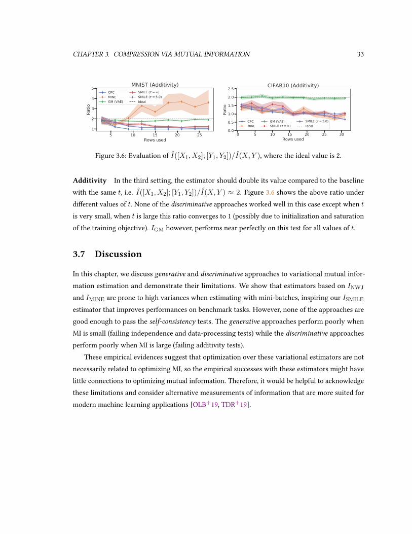
CHAPTER 3. COMPRESSION VIA MUTUAL INFORMATION 33
5 10 15 20 25Rows used
1
2
3
4
5Ra
tioMNIST (Additivity)
CPCMINEGM (VAE)
SMILE (τ= ∞)SMILE (τ= 5.0)Ideal
0 5 10 15 20 25 30Rows used
0.0
0.5
1.0
1.5
2.0
2.5
Ratio
CIFAR10 (Additivity)
CPCMINE
GM (VAE)SMILE (τ= ∞)
SMILE (τ= 5.0)Ideal
Figure 3.6: Evaluation of I([X1, X2]; [Y1, Y2])/I(X,Y ), where the ideal value is 2.
Additivity In the third setting, the estimator should double its value compared to the baselinewith the same t, i.e. I([X1, X2]; [Y1, Y2])/I(X,Y ) ≈ 2. Figure 3.6 shows the above ratio underdierent values of t. None of the discriminative approaches worked well in this case except when tis very small, when t is large this ratio converges to 1 (possibly due to initialization and saturationof the training objective). IGM however, performs near perfectly on this test for all values of t.
3.7 Discussion
In this chapter, we discuss generative and discriminative approaches to variational mutual infor-mation estimation and demonstrate their limitations. We show that estimators based on INWJ
and IMINE are prone to high variances when estimating with mini-batches, inspiring our ISMILE
estimator that improves performances on benchmark tasks. However, none of the approaches aregood enough to pass the self-consistency tests. The generative approaches perform poorly whenMI is small (failing independence and data-processing tests) while the discriminative approachesperform poorly when MI is large (failing additivity tests).
These empirical evidences suggest that optimization over these variational estimators are notnecessarily related to optimizing MI, so the empirical successes with these estimators might havelittle connections to optimizing mutual information. Therefore, it would be helpful to acknowledgethese limitations and consider alternative measurements of information that are more suited formodern machine learning applications [OLB+19, TDR+19].

Chapter 4
Representation Learning viaClassication
In the previous chapter, we have discussed the limitations of existing variational mutual informationestimators and how we can improve the estimation by variance reduction. However, being able toaccurately estimate mutual information is not enough for unsupervised representation learning,since we often would like to maximize the informativeness of the representations eciently.
In this chapter, we discuss how we can pose unsupervised representation learning as a multi-label classication problem. Variational mutual information (MI) estimators are widely used inunsupervised representation learning methods such as contrastive predictive coding (CPC). A lowerbound on MI can be obtained from a multi-class classication problem, where a critic attempts todistinguish a positive sample drawn from the underlying joint distribution from (m− 1) negativesamples drawn from a suitable proposal distribution. Using this approach, MI estimates are boundedabove by logm, and could thus severely underestimate unless m is very large.
To overcome this limitation, we introduce a novel estimator based on a multi-label classicationproblem, where the critic needs to jointly identify multiple positive samples at the same time.We show that using the same amount of negative samples, multi-label CPC is able to exceed thelogm bound, while still being a valid lower bound of mutual information. We demonstrate thatthe proposed approach is able to lead to better mutual information estimation, gain empirical im-provements in unsupervised representation learning, and beat a current state-of-the-art knowledgedistillation method over 10 out of 13 tasks.
This chapter was previous published as [SE20b].
34

CHAPTER 4. REPRESENTATION LEARNING VIA CLASSIFICATION 35
4.1 Introduction
Learning ecient representations from data with minimal supervision is a critical problem inmachine learning with signicant practical impact [MSC+13, DCLT18, MK13, RNSS18, BMR+20].Representations obtained using large amounts of unlabeled data can boost performance on down-stream tasks where labeled data is scarce. This paradigm is already successful in a variety ofdomains; for example, representations trained on large amounts of unlabeled images can be usedto improve performance on detection [ZZY19, HFW+19, CKNH20].
In the context of learning visual representations, contrastive objectives based on variationalmutual information (MI) estimation are among the most successful ones [vdOLV18, BBR+18,DHFLM+18, POvdO+19, TKI19]. One such approach, named Contrastive Predictive Coding (CPC,[vdOLV18]), obtains a lower bound to MI via a multi-class classication problem. In CPC, a criticis generally trained to distinguish a pair of representations from two augmentations of the sameimage (positive), apart from (m− 1) pairs of representations from dierent images (negative). Therepresentation network is then trained to increase the MI estimates given by the critic. This bringstogether the two representations from the positive pair and pushes apart the two representationsfrom the negative pairs.
It has been empirically observed that factors leading to better MI estimates, such as trainingfor more iterations and increasing the complexity of the critic [CKNH20, CFGH20], can generallyresult in improvements over downstream tasks. In the context of CPC, increasing the numberof negative samples per positive sample (i.e. increasing m) also helps with downstream perfor-mance [WXYL18, HFW+19, CKNH20, TKI19]. This can be explained from a mutual informationestimation perspective that CPC estimates are upper bounded by logm, so increasing m could re-duce bias when the actual mutual information is much higher [MC18]. However, due to constraintsover compute, memory and data, there is a limit to how many negative samples we can obtain perpositive sample.
In this chapter, we propose generalizations to CPC that can increase the logm bound withoutadditional computational costs, thus decreasing bias. We rst generalize CPC through by re-weighting the inuence of positive and negative samples in the underlying the classicationproblem. This increases the logm bound and leads to bias reduction, yet the re-weighted CPCobjective is no longer guaranteed to be a lower bound to mutual information.
To this end, we introduce multi-label CPC (ML-CPC) which poses mutual information estima-tion as a multi-label classication problem. Instead of identifying one positive sample for each

CHAPTER 4. REPRESENTATION LEARNING VIA CLASSIFICATION 36
classication task (as in CPC), the critic now simultaneously identies multiple positive samplesthat come from the same batch. We prove for ML-CPC that under certain choices of the weights,we can increase the logm bound and reduce bias, while guaranteeing that the new objective isstill lower bounded by mutual information. This provides an practical algorithm whose upperbound is close to the theoretical upper limit by any distribution-free, high-condence lower boundestimators of mutual information [MS20].
Re-weighted ML-CPC encompasses a range of mutual information lower bound estimatorswith dierent bias-variance trade-os, which can be chosen with minimal impact on the computa-tional costs. We demonstrate the eectiveness of re-weighted ML-CPC over CPC empirically onseveral tasks, including mutual information estimation, knowledge distillation and unsupervisedrepresentation learning. In particular, ML-CPC is able to beat the current state-of-the-art methodin knowledge distillation [TKI19] on 10 out of 13 distillation tasks for CIFAR-100.
4.2 Contrastive Predictive Coding and Mutual Information
Oord et al. [vdOLV18] interpreted the CPC objective as a lower bound to MI, but only proved thecase for a lower bound approximation of CPC, where a term containing −E[log g] is replaced by− logE[g]; so their arguments alone cannot prove that CPC is a lower bound of mutual information.Poole et al. [POvdO+19] proved a lower bound argument for the objective where m = n andnegative samples are tied to other positive samples in the same batch. To bridge the gap betweentheory (that CPC instantiates InfoMax) and practice (where negative samples can be chosenindependently from positive samples of the same batch, such as MoCo [HFW+19]), we presentanother proof for the general CPC objective as presented in L(g). First, we show the followingresult for variational lower bounds of KL divergences between general distributions where batchesof negative samples are used to estimate the divergence. Then, as mutual information is a KLdivergence between two specic distributions, the lower bound argument for CPC simply follows.
Theorem 5. For all probability measures P,Q over sample space X such that P Q, the following
holds for all functions r : X → R+ and integersm ≥ 2:
DKL(P‖Q) ≥ Ex∼P,y1:m−1∼Qm−1
[log
m · r(x)
r(x) +∑m−1
i=1 r(yi)
]. (4.1)
Proof. In Appendix A.2, using the variational representations of f -divergences [NWJ08] and Prop. 6.

CHAPTER 4. REPRESENTATION LEARNING VIA CLASSIFICATION 37
The argument about CPC being a lower bound to MI is simply a corollary of the above statementwhere P is p(x,y) (joint) and Q is p(x)p(y) (product of marginals); we state the claim below.
Corollary 2. ∀n ≥ 1,m ≥ 2, ∀g : X × Y → R+, the following is true: L(g) ≤ I(X;Y ).
Therefore, one can train g and h to maximize L(g) (recall that L depends on h via y = h(x)),which is guaranteed to be lower than I(X;Y ) in expectation.
CPC is an estimator with high bias For nitem, since g(xi,yi) appears in both the numeratorand denominator of Equation 2.16 and g is positive, the density ratio estimates can be no largerthan m, and the value of L(g) is thus upper bounded by logm [vdOLV18]. While this is acceptablefor certain low dimensional scenarios, this can lead to high-bias if the true mutual information ismuch larger than logm. In fact, the required m can be unacceptable in high dimensions since MIcan scale linearly with dimension, which means an exponential number of negative samples areneeded to achieve low bias.
For example, ifX and Y are 1000-dimensional random variables where the marginal distributionfor each dimension is standard Gaussian, and for each dimension d, Xd and Yd has a correlation of0.2, then the mutual information I(X;Y ) is around 20.5, which means that m has to be greaterthan 4 × 10⁸ in order for CPC estimates to approach this value. In comparison, state-of-the-artimage representation learning methods use am that is around 65536 and representation dimensionsbetween 128 to 2048 [WXYL18, HFW+19, CKNH20] due to batch size and memory limitations, asone would need a sizeable batch of positive samples in order to apply batch normalization [IS15].
4.2.1 Re-weighted Contrastive Predictive Coding
Under the computational limitations imposed by m (i.e., we cannot obtain too many negativesamples per positive sample), we wish to develop generalizations to CPC that reduce bias whilestill being lower bounds to the mutual information. We do not consider other types of estimatorssuch as MINE [BBR+18] or NWJ [NWJ08] because they would exhibit high variance on the orderof O(eI(X;Y )) [SE19b], and thus are much less stable to optimize.
One possible approach is to decrease the weights of the positive sample when calculating thesum in the denominator; this leads to the following objective, called α-CPC:
Lα(g) := E
[1
n
n∑i=1
logm · g(xi,yi)
αg(xi,yi) + m−αm−1
∑m−1j=1 g(xi,yi,j)
](4.2)

CHAPTER 4. REPRESENTATION LEARNING VIA CLASSIFICATION 38
where the positive sample is weighted by α and negative samples are weighted by m−αm−1 . The
purpose of adding weights to negative samples is to make sure the the weights sum to m, like inthe original case where each sample has weight 1 and there are m samples in total. Clearly, theoriginal CPC objective is a special case when α = 1.
On the one hand, Lα(g) is now upper bounded by log mα , which is larger than logm when
α ∈ (0, 1). Thus, α-CPC has the potential to reduce bias when logm is much smaller than I(X;Y ).On the other hand, when we set a smaller α, the variance of the estimator becomes larger, and theobjective Lα(g) becomes more dicult to optimize [HLLT16, HLCT19]. Therefore, selecting anappropriate α to balance the bias-variance trade-o is helpful for optimization of the objective inpractice.
However, it is now possible for Lα(g) to be larger than I(X;Y ) as the number of classesm grows to innity, so optimizing Lα(g) does not necessarily recover a lower bound to mutualinformation. We illustrate this via the following example (more details in Appendix B.2.2).
Example 1. LetX,Y be two binary r.v.s such that Pr(X = 1, Y = 1) = Pr(X = 0, Y = 0) = 0.5.
Then I(X;Y ) = log 2 ≈ 0.69. However, when α = 0.5 and n = m = 3, we can analytically
compute Lα(g) ≈ 0.72 ≥ I(X;Y ) for g(x, y) = 1 if x = y and near 0 otherwise.
4.3 Multi-label Contrastive Predictive Coding
While α-CPC could be useful empirically, we lack a principled way of selecting proper values ofα as Lα(g) may no longer be a lower bound to mutual information. In the following sections,we propose an approach that allows us to achieve both, i.e., for all α in a certain range (that onlydepends on n and m), we can achieve an upper bound of log m
α while ensuring that the objective isstill a lower bound on mutual information. This allows us to select dierent values of α to reectdierent preferences over bias and variance, all while keeping the computational cost identical.
We consider solving a “nm-class, n-label” classication problem, where given n positive samplesand n(m− 1) negative samples yj,k ∼ p(y), we wish to jointly identify the top-n samples that aremost likely to be the positive ones. Concretely, this has the following objective function:
J(g) := E
[1
n
n∑i=1
lognm · g(xi,yi)∑n
j=1 g(xj ,yj) +∑n
j=1
∑m−1k=1 g(xj ,yj,k)
](4.3)
where the expectation is taken over the n positive samples (xi,yi) ∼ p(x,y) for i ∈ [n] andthe n(m − 1) negative samples yj,k ∼ p(y) for j ∈ [n], k ∈ [m − 1]. We call this multi-label

CHAPTER 4. REPRESENTATION LEARNING VIA CLASSIFICATION 39
contrastive predictive coding (ML-CPC), since the classier now needs to predict n positive labelsfrom nm options at the same time, instead of 1 positive label from m options as in traditional CPC(performed for n times for a batch size of n).
Distinctions fromCPC Despite its similarity compared to CPC (both are based on classication),we note that the multi-label perspective is fundamentally dierent from the CPC paradigm in threeaspects, and cannot be treated as simply increasing the number of negative samples.
1. The ML-CPC objective value depends on the batch size n, whereas the CPC objective doesnot.
2. In CPC the positive pair and negative pairs share a same element (xi in equation 2.16 wherethe positive sample is (xi,yi)), whereas in ML-CPC the negative pairs no longer have suchrestrictions; this could be useful for smaller datasetsD when the number of possible negativepairs increases from O(|D|) to O(|D|2).
3. The optimal critic for CPC is g? = c(x)·p(x,y)/(p(x)p(y)), where c is any positive functionof x [MC18]. In ML-CPC, dierent x values are tied within the same batch, so the optimalcritic for ML-CPC is g? = c · p(x,y)/(p(x)p(y)), where c is a positive constant. As a result,ML-CPC reduces the amount of optimal solutions, and forces the similarity of any positivepair to be higher than that of any negative pair, unlike CPC where the positive pair onlyneeds to have higher similarity than any negative pairs with the same x.
Computational cost of ML-CPC To compute CPC with a batch size of n, one would neednm critic evaluations and compute n sums in the denominator, each over a dierent set of mevaluations. To compute ML-CPC, one needs nm critic evaluations, and compute 1 sum over all nmevaluations. Therefore, ML-CPC has almost the same computational cost compared to CPC whichis O(mn). We perform a similar analysis in Appendix A.2 to show that evaluating the gradients ofthe objectives also has similar costs, so ML-CPC is computationally as ecient as CPC.
4.3.1 Re-weighted Multi-label Contrastive Predictive Coding
Similar to α-CPC, we can modify the multi-label objective J(g) by re-weighting the critic predic-tions, which results in the following objective called α-ML-CPC:
Jα(g) := E
[1
n
n∑i=1
lognm · g(xi,yi)
α∑n
j=1 g(xj ,yj) + m−αm−1
∑nj=1
∑m−1k=1 g(xj ,yj,k)
](4.4)

CHAPTER 4. REPRESENTATION LEARNING VIA CLASSIFICATION 40
For α ∈ (0, 1), we down-weight the positive critic outputs by α and up-weight the negative criticoutputs by m−α
m−1 (similar to α-CPC). Setting a smaller α has the potential to reduce bias, since theupper bound of logm is changed to log m
α , which is larger when α ∈ (0, 1). In contrast to α-CPC,Jα(g) is now guaranteed to be a lower bound of mutual information for a wide range of α, aswe show in the following statements. Similar to the case of CPC, we rst show a more generalargument, for which the weighted ML-CPC is a special case.
Theorem 6. For all probability measures P,Q over sample space X such that P Q, the following
holds for all functions r : X → R+, integers n ≥ 1,m ≥ 2, and real numbers α ∈ [ mn(m−1)+1 , 1]:
DKL(P‖Q) ≥ Ex1:n∼Pn,yi,1:m−1∼Qm−1
[1
n
n∑i=1
logmn · r(xi)
α∑n
j=1 r(xj) + m−αm−1
∑m−1k=1 r(yj,k)
].
(4.5)
Proof. In Appendix A.2, using the variational representations of f -divergences [NWJ08] and Prop. 7.
The above theorem extends existing variational lower bound estimators of KL divergences (thatare generally interpreted as binary classication [SSK12, NWJ08]) into a family of lower boundsthat can be interpreted as multi-label classication. The argument about re-weighted ML-CPCbeing a lower bound to MI is simply a corollary where P is p(x,y) and Q is p(x)p(y); we statethe claim below.
Corollary 3. ∀n ≥ 1,m ≥ 2, dene αm,n = mn(m−1)+1 . If α ∈ [αm,n, 1], then ∀g : X × Y → R+,
Jα(g) ≤ I(X;Y ) (4.6)
The above theorem shows that for an appropriate range of α values, the objective Jα(g) is stillguaranteed to be a variational lower bound to mutual information, like the original CPC objective.Selecting α within this range results in estimators with dierent bias-variance trade-os. Here, asmaller α could lead to low-bias high-variance estimates; this achieves a similar eect to increasingthe number of classes m to nearly m/α, but without the actual additional computational costs thatcomes with obtaining more negative samples in CPC.
Illustrative example We consider the case of X,Y being binary and equal random variablesin Example 1, where I(X;Y ) = log 2 ≈ 0.69, the optimal critic g is known, and both Lα(g) and

CHAPTER 4. REPRESENTATION LEARNING VIA CLASSIFICATION 41
0.0 0.2 0.4 0.6 0.8 1.00.5
1.0
1.5
Estim
ates
m = 3-CPC-ML-CPC
True MIm, n
0.0 0.2 0.4 0.6 0.8 1.0
0.6
0.8
1.0
Estim
ates
m = 5
0.0 0.2 0.4 0.6 0.8 1.00.60
0.65
0.70
0.75
Estim
ates
m = 10
Figure 4.1: MI estimates with CPC and ML-CPC under dierent α.
0 20 40 60 80 100# of classes m
10 4
10 2
Bias
0 20 40 60 80 100# of classes m
10 3
10 1Variance
CPCm, n-ML-CPC
Figure 4.2: Bias-variance trade-os for dierentm. Lower is better.
Jα(g) can be computed in closed-form for any α and g in O(m) time (details in Appendix B.2.2).We plot the CPC (equation 4.2) and ML-CPC (equation 4.4) objectives with dierent choices of αand m in Figure 4.1. The estimates of ML-CPC when α ≥ αm,n are lower bounds to the groundtruth MI, which indeed aligns with our theory.
Furthermore, in Figure 4.2 we illustrate the bias-variance trade-os for CPC and αm,n-ML-CPCas we vary the number of classes m (for simplicity, we choose n = m). Despite having slightlyhigher variance in the estimates, αm,n-ML-CPC has signicantly less bias than CPC, which suggeststhat it is helpful in cases where lower bias is preferable than lower variance. In practice, the usercould select dierent values of α to indicate the desired trade-o, all without having to change thenumber of negative samples and increase computational costs.
We include the pseudo-code and a PyTorch implementation to α-ML-CPC in Appendix B.2.1.
4.4 Related Work
Contrastive methods for representation learning The general principle of contrastive meth-ods for representation learning encourages representations to be closer between “positive” pairsand further between “negative” pairs, which has been applied to learning representations in vari-ous domains such as images [HRD+19, WXYL18, HFW+19, CKNH20], words [MSC+13, DCLT18],graphs [VFH+18] and videos [HXZ19]. Commonly used objectives include the logistic loss [MSC+13],margin triplet loss [SKP15], the noise contrastive estimation loss [GH12] and other objectives based

CHAPTER 4. REPRESENTATION LEARNING VIA CLASSIFICATION 42
on variational lower bounds of mutual information, such as MINE [BBR+18] and CPC [vdOLV18].CPC-based approaches have gained interest due to its superior performance in downstream taskscompared to other losses such as the logistic and margin loss [CKNH20].
Variational mutual information estimators Estimating mutual information from samples ischallenging [MS20, XZS+20]. Most variational approaches to mutual information estimation arebased on the Fenchel dual representation of f -divergences [NWJ08, SE19a], where a critic functionis trained to learn the density ratio p(x,y)/(p(x)p(y)). These approaches mostly vary in terms ofhow the critics are modeled and optimized [BA03, POvdO+19], and exhibit dierent bias-variancetrade-os from these choices.
CPC would tend to underestimate the density ratio (since it is capped at m) and generallyrequiresO(eI(X;Y )) samples to achieve low bias; MINE [BBR+18] (based on the Donsker-Varadhaninequality [DV75]) is a biased estimator and requires O(eI(X;Y )) samples to achieve low vari-ance [SE19b, SE19a]. Poole et al. [POvdO+19] proposed an estimator that interpolates between twotypes of estimators, allowing for certain bias-variance trade-os; this is relevant to our proposedre-weighted CPC in the sense that positive samples are down-weighted, but an additional baselinemodel is required during training. Through ML-CPC, we introduce a family of unbiased mutualinformation lower bound estimators, and reect a wide range of bias-variance trade-os withoutusing more negative samples.
Relevance to the limitations of mutual information lower bound estimators Further-more, we note that ML-CPC is upper bounded by log(n(m− 1) + 1) for the smallest possible α,which appears to be very close to (but smaller than) the general upper limit of O(log nm) that canbe achieved by any distribution-free high-condence lower bound (namely, estimates from samplesare lower bounds to the true mutual infomation with high probability) on mutual information fornm samples [MS20]. However, we note that the assumptions in [MS20] are slightly dierent toour settings, in the sense that they assumed complete access to the distribution p(x,y) and onlyrequired samples from p(x)p(y), whereas we have to estimate p(x,y) from the samples as well;and the amount of samples we obtain from p(x)p(y) is n(m− 1) instead of nm. We hypothesizethat we can reach the theoretical limit with a method derived from ML-CPC, but leave it as aninteresting future direction.
Re-weighted softmax loss Generalizations to the softmax loss have been proposed in whichdierent weights are assigned to dierent classes or samples [LWYY16, LLW17, WLLC18], which

CHAPTER 4. REPRESENTATION LEARNING VIA CLASSIFICATION 43
are commonly used with regularization [BL18]. When the dataset has extremely imbalanced classes,higher weights are given to classes with less frequency [HLLT16, HLCT19, WRH17] or classeswith less eective samples [CJL+19]. Cao et al. [CWG+19] investigate re-weighting approachesthat encourages large margins to the decision boundary for minority classes; such a context isalso studied for detection [LKG19] and segmentation [KHZ+19] where class imbalance exists. Ourwork introduce re-weighting approaches to the context of unsupervised representation learning(where class labels do not exist in the traditional sense), where we aim for exible bias-variancetrade-os in contrastive mutual information estimators.
4.5 Experiments
We evaluate our proposed methods on mutual information estimation, knowledge distillationand unsupervised representation learning. To ensure fair comparisons are made, we only make
adjustments to the training objective, and keep the remaining experimental setup identical to that of
the baselines. We describe details to the experimental setup in Appendix B.2.2. Our code is availableat https://github.com/jiamings/ml-cpc.
0 5000 10000 15000 20000Steps
0
2
4
6
8
10
MI (
nats
)
CPC ( = 1.0)Joint criticSeparable criticTrue MIlog(bs)
0 5000 10000 15000 200000
2
4
6
8
10
CPC ( = 0.1)
0 5000 10000 15000 200000
2
4
6
8
10
CPC ( = 0.01)
0 5000 10000 15000 200000
2
4
6
8
10
CPC ( = 0.001)
0 5000 10000 15000 200000
2
4
6
8
10
CPC ( = 0.0001)
0 5000 10000 15000 20000Steps
0
2
4
6
8
10
MI (
nats
)
ML-CPC ( = 1.0)Joint criticSeparable criticTrue MIlog(bs)
0 5000 10000 15000 200000
2
4
6
8
10
ML-CPC ( = 0.1)
0 5000 10000 15000 200000
2
4
6
8
10
ML-CPC ( = 0.01)
0 5000 10000 15000 200000
2
4
6
8
10
ML-CPC ( = 0.001)
0 5000 10000 15000 200000
2
4
6
8
10
ML-CPC ( = 0.0001)
Figure 4.3: Mutual information estimation with CPC and ML-CPC, with dierent choices of α.
4.5.1 Mutual Information Estimation
Setup We rst consider mutual information estimation between two correlated Gaussians of 20dimensions, following the setup in [POvdO+19, SE19b] where the ground truth mutual informationis known and increases by 2 every 4k iterations, for a total of 20k iterations. We evaluate CPC and

CHAPTER 4. REPRESENTATION LEARNING VIA CLASSIFICATION 44
ML-CPC with dierent choices of α (ranging from 1.0 to 0.0001, which might not guarantee thatthey are lower bounds to mutual information) under two types of critic, named joint [BBR+18]and separable [vdOLV18]. We use m = n = 128 in our experiments.
Results We illustrate the estimates and the ground truth MI in Figure 4.3. Both CPC and ML-CPCestimates are bounded by logm when α = 1, which is no longer the case when we set smallervalues of α; however, as we decrease α, CPC estimates are no longer guaranteed to be lower boundsto mutual information, whereas ML-CPC estimates still provide lower bound estimates in general.Moreover, a reduction in α for ML-CPC reduces bias at the cost of increasing variance, as theproblem becomes more dicult with re-weighting. The time to compute 200 updates on a Nvidia1080 Ti GPU with the a PyTorch implementation is 1.15± 0.06 seconds with CPC and 1.14± 0.04
seconds with ML-CPC, so the computational costs are indeed near identical.
4.5.2 Knowledge Distillation
Setup We apply re-weighted CPC and ML-CPC to knowledge distillation (KD, [HVD15]), inwhich one neural network model (teacher) transfers its knowledge to another model (student,typically smaller) so that the student’s performance is higher than training from labels alone.Contrastive representation distillation (CRD, [TKI19]) is a state-of-the-art method that regularizesthe student model so that its features have higher mutual information with that of the teacher;CRD is implemented via a type of noise contrastive estimation objective [GH12]. We replace thisobjective with CPC and ML-CPC, using dierent choices of α that are xed throughout training,and keeping the remaining hyperparameters identical to the CRD ones in [TKI19]. Two baselines areconsidered: the original KD objective in [HVD15] and the state-of-the-art CRD objective in [TKI19],since other baselines [KKBZ19, AHD+19, HW17, KPK18] are shown to have inferior performancein general.
Results Following the procedure in [TKI19], we evaluate over 13 dierent student-teacher pairson CIFAR-100 [KH+09]. The student and teacher have the same type of architecture in 7 casesand dierent types in 6 cases. We report top-1 test accuracy in Table 4.1 (same type) and Table 4.2(dierent types), where each case is the mean evaluation from 3 random seeds. We omit the standarddeviation across dierent random seeds of each setup to t the table in the paper, but we notethat deviation among dierent random seeds is fairly small (at around 0.05 to 0.1 for most cases).While CPC and ML-CPC are generally inferior to that of CRD when α = 1.0 (this aligns with the

CHAPTER 4. REPRESENTATION LEARNING VIA CLASSIFICATION 45
0.0 0.2 0.4 0.6 0.8 1.0
73.6
73.7
Top-
1 Ac
cura
cy
Same Type (Average)
0.0 0.2 0.4 0.6 0.8 1.0
73.2
73.4
73.6
Top-
1 Ac
cura
cy
Different Types (Average)CPCML-CPCCRD
Figure 4.4: Ablation studies for knowledge distillation with CPC and ML-CPC at dierentvalues of α. Left: student and teacher are of the same type. Right: student and teacher are fromdierent types.
observation in [TKI19]), they outperform CRD in 10 out of 13 cases when a smaller α is selected.To demonstrate the eect of improved performance of smaller α, we evaluate average top-
1 accuracies with α ∈ 0.01, 0.05, 0.1, 0.2, 0.5, 1.0 in Figure 4.4. Both CPC and ML-CPC aregenerally inferior to CRD when α = 1.0 or 0.5, but as we select smaller values of α, they becomesuperior to CRD and reaches the highest values at around 0.01 to 0.05, with ML-CPC being slightlybetter. Moreover, n = 64,m = 16384 so αm,n ≈ 0.015, which achieves the lowest bias whileensuring ML-CPC to be a lower bound to MI. Thus this observation aligns with our claims on αm,nin Theorem 3.
Table 4.1: Top-1 test accuracy (%) of students networks on CIFAR100 where the student and teachernetworks are of the same type. (↑) and (↓) denotes superior and inferior performance relative toCRD. Each result is the mean of 3 random runs. Lα and Jα denote α-CPC and α-ML-CPC.
Teacher WRN-40-2 WRN-40-2 resnet56 resnet110 resnet110 resnet32x4 vgg13Student WRN-16-2 WRN-40-1 resnet20 resnet20 resnet32 resnet8x4 vgg8
Teacher 75.61 75.61 72.34 74.31 74.31 79.42 74.64Student 73.26 71.98 69.06 69.06 71.14 72.50 70.36
KD 74.92 73.54 70.66 70.67 73.08 73.33 72.98CRD 75.48 74.14 71.16 71.46 73.48 75.51 73.94
L1.0 75.42 (↓) 74.16 (↑) 71.32 (↑) 71.39 (↓) 73.57 (↑) 75.50 (↓) 73.60 (↓)L0.1 75.69 (↑) 74.17 (↑) 71.48 (↑) 71.38 (↓) 73.66 (↑) 75.41 (↓) 73.61 (↓)J1.0 75.39 (↓) 74.18 (↑) 71.28 (↑) 71.28 (↓) 73.58 (↑) 75.32 (↓) 73.67 (↓)J0.05 75.64 (↑) 74.27 (↑) 71.33 (↑) 71.24 (↓) 73.57 (↑) 75.50 (↓) 74.01 (↑)J0.01 75.83 (↑) 74.24 (↑) 71.50 (↑) 71.27 (↓) 73.90 (↑) 75.37 (↓) 73.95 (↑)

CHAPTER 4. REPRESENTATION LEARNING VIA CLASSIFICATION 46
Table 4.2: Top-1 test accuracy (%) of students networks on CIFAR100 where the student and teachernetworks are from dierent types. (↑) and (↓) denotes superior and inferior performance relative toCRD. Each result is the mean of 3 random runs. Lα and Jα denote α-CPC and α-ML-CPC.
Teacher vgg13 ResNet50 ResNet50 resnet32x4 resnet32x4 WRN-40-2Student MobileNetV2 MobileNetV2 vgg8 ShueNetV1 ShueNetV2 ShueNetV1
Teacher 74.64 79.34 79.34 79.42 79.42 75.61Student 64.60 64.60 70.36 70.50 71.82 70.50
KD 67.37 67.35 73.81 74.07 74.45 74.83CRD 69.73 69.11 74.30 75.11 75.65 76.05
L1.0 69.24 (↓) 69.02 (↓) 73.66 (↓) 75.00 (↓) 75.93 (↑) 75.72 (↓)L0.1 69.26 (↓) 69.33 (↑) 74.24 (↓) 75.34 (↑) 76.01 (↑) 76.12 (↑)J1.0 68.92 (↓) 68.80 (↓) 73.65 (↓) 75.39 (↑) 75.88 (↑) 75.70 (↓)J0.05 69.25 (↓) 70.04 (↑) 74.84 (↑) 75.51 (↑) 76.24 (↑) 76.03 (↑)J0.01 69.25 (↓) 69.90 (↑) 74.81 (↑) 75.47 (↑) 76.04 (↑) 76.19 (↑)
4.5.3 Representation Learning
Setup Finally, we consider ML-CPC for unsupervised representation learning as a replacement toCPC. We follow the experiment procedures in MoCo-v2 [CFGH20] (which used the CPC objective),where negative samples are obtained from a key encoder that updates more slowly than therepresentation network. We use the “linear evaluation protocol” where the learned representationsare evaluated via the test top-1 accuracy when a linear classier is trained to predict labels fromrepresentations. Dierent from knowledge distillation, we do not have labels and xed teacherrepresentations, so the problem becomes much more dicult and using small values of α alonewill lead to high variance in initial estimates which could hinder the nal performance. To thisend, we use a curriculum learning [BLCW09] approach where we select α values from high tolow throughout training: higher α has higher bias, lower variance and easier to learn, whereaslower α has lower bias, higher variance and harder to learn. For ML-CPC, we consider 4 types ofgeometrically decreasing schedules for α: xed at 1.0; from 2.0 to 0.5; from 5.0 to 2.0; and from10.0 to 0.1; so α = 1.0 for all cases when we reached half of the training epochs. We use the samevalues for other hyperparameters as those used in the MoCo-v2 CPC baseline (more details inAppendix B.2.2).
Results We show the top-1 accuracy of the learned representations under the linear evaluationprotocol in Table 4.3 for CIFAR10 and CIFAR100. While the original ML-CPC objective (denoted

CHAPTER 4. REPRESENTATION LEARNING VIA CLASSIFICATION 47
as J1.0 → J1.0) already outperforms the CPC baseline in most cases, we observe that using acurriculum from easy to hard objective has the potential to further improve performance of therepresentations. Notably, the J10.0 → J0.1 schedule improves the performance on both datasets byalmost 2.5 percent when trained for 200 epochs, which demonstrates its eectiveness when thenumber of epochs used during training is limited.
Table 4.3: Top-1 accuracy of unsupervised representation learning.
(a) CIFAR-10
Epochs 200 500 1000
L1.0 83.28 89.31 91.20
J1.0 → J1.0 83.61 (↑) 89.43 (↑) 91.48 (↑)J2.0 → J0.5 84.31 (↑) 89.47 (↑) 91.43 (↑)J5.0 → J0.2 85.52 (↑) 89.85 (↑) 91.50 (↑)J10.0 → J0.1 86.16 (↑) 89.49 (↑) 91.86 (↑)
(b) CIFAR-100
Epochs 200 500 1000
L1.0 61.42 67.72 69.63
J1.0 → J1.0 61.80 (↑) 67.68 (↓) 70.85 (↑)J2.0 → J0.5 62.92 (↑) 68.01 (↑) 70.22 (↑)J5.0 → J0.2 63.58 (↑) 68.04 (↑) 70.07 (↑)J10.0 → J0.1 64.05 (↑) 67.94 (↑) 70.03 (↑)
In Table 4.4, we include additional results for ImageNet under a compute-constrained scenario,where the representations are trained for only 30 epochs on a ResNet-18 architecture. Similar tothe observations in CIFAR-10, we observe improvements in terms of linear classication accuracyof the learned representations. This demonstrates that the curriculum learning approach (specicto ML-CPC with re-weighting schedules, where the objective remains a lower bound to mutualinformation) could be useful to unsupervised representation learning in general.
4.6 Discussion
In this chapter, we proposed multi-label contrastive predictive coding for representation learning,which provides a generalization to contrastive predictive coding via multi-label classication. Re-weighted ML-CPC is able to enjoy less bias while being a lower bound to mutual information. Ourupper bounds for the smallest α is close to the theoretical limit [MS20] of any distribution-free high-condence lower bound on mutual information estimation. We demonstrate the eectiveness of
Table 4.4: ImageNet representation learning for 30 epochs.
Objective L1.0 J1.0 → J1.0 J2.0 → J0.5 J5.0 → J0.2 J10.0 → J0.1
Top1 43.45 43.24 (↓) 43.52 (↑) 43.86 (↑) 43.81 (↑)Top5 67.42 67.43 (↑) 67.82 (↑) 67.67 (↑) 67.71 (↑)

CHAPTER 4. REPRESENTATION LEARNING VIA CLASSIFICATION 48
ML-CPC on mutual information, knowledge distillation and unsupervised representation learning.It would be interesting to further apply this method to other application domains, investigate al-
ternative methods to control the re-weighting procedure (such as using angular margins [LWYY16]),and develop more principled approaches towards curriculum learning for unsupervised represen-tation learning. From a theoretical standpoint, it is also interesting to formally investigate thebias-variance trade-o of ML-CPC, and see whether simple modications to ML-CPC based on aslightly dierent assumption over p(x,y) could approach the theoretical limit by McAllester andStratos [MS20].

Chapter 5
Fair Representation Learning viaRegression
In the previous chapter, our goal was to learn compressed representations of the data that are asinformative as possible. However, in many real-world applications, raw data often contain certainsensitive information, such as age and gender. If we wish to protect the user from data misuse, thenremoving the sensitive information alone would not be enough: one can still infer the sensitiveattributes from other features (for example, one’s favorite activity could be correlated to theirgender). This motivates us to produce not only informative representations, but also “fair” onesthat reduces the undesirable information about sensitive information.
In this chapter, we propose an information-theoretically motivated objective for learning maxi-mally expressive fair representations. We unify a range of existing approaches by showing theyoptimize approximations to the Lagrangian dual of our objective. These existing approaches maylearn somewhat expressive and fair representations, but users wanting to control the fairness ofrepresentations must tune the expressiveness-fairness trade-o over many runs and will neverknow whether they have obtained the maximally expressive representations under certain fair-ness constraints. We are the rst to provide user control over the fairness of representationsthrough a user-speciable limit on unfairness. Through a dual optimization method (optimizingthe model as well as the expressiveness-fairness trade-o), we obtain representations achievinghigh expressiveness while satisfying the user-specied limits on unfairness.
This chapter was previous published as [SKG+19]. Pratyusha Kalluri, Aditya Grover andShengjia Zhao contributed to the contents of this chapter. My contributions are conceiving the idea,implementing the algorithm, executing the experiments and writing the chapter. Other coauthors
49

CHAPTER 5. FAIR REPRESENTATION LEARNING VIA REGRESSION 50
helped with discussions and writing.
5.1 Introduction
Statistical learning systems are increasingly being used to assess individuals, inuencing conse-quential decisions such as bank loans, college admissions, and criminal sentences. This yields agrowing demand for systems guaranteed to output decisions that are fair with respect to sensitiveattributes such as gender, race, and disability.
In the typical classication and regression settings with fairness and privacy constraints, oneis concerned about performing a single, specic task. However, situations arise where a dataowner needs to release data to downstream users without prior knowledge of the tasks that willbe performed [MCPZ18]. In such cases, it is crucial to nd representations of the data that can beused on a wide variety of tasks while preserving fairness [CWRV17].
This gives rise to two desiderata. On the one hand, the representations need to be expressive, sothat they can be used eectively for as many tasks as possible. On the other hand, the representationsalso need to satisfy certain fairness constraints to protect sensitive attributes. Further, many notionsof fairness are possible, and it may not be possible to simultaneously satisfy all of them [KMR16,Cho17]. Therefore, the ability to eectively trade o multiple notions of fairness is crucial to fairrepresentation learning.
To this end, we present an information theoretically motivated constrained optimization frame-work (Section 5.2). The goal is to maximize the expressiveness of representations while satisfy-ing certain fairness constraints. We represent expressiveness as well as three dominant notionsof fairness (demographic parity [ZWS+13], equalized odds, equalized opportunity [HPS16]) interms of mutual information, obtain tractable upper/lower bounds of these mutual informationobjectives, and connect them with existing objectives such as maximum likelihood, adversarialtraining [GPAM+14], and variational autoencoders [KW13, RM15].
As we demonstrate in Section 5.3, this serves as a unifying framework for existing work [ZWS+13,LSL+15, ES15, MCPZ18] on learning fair representations. A range of existing approaches to learningfair representations, which do not draw connections to information theory, optimize an approx-imation of the Lagrangian dual of our objective with xed values of the Lagrange multipliers.These thus require the user to obtain dierent representations for dierent notions of fairness asin [MCPZ18].
Instead, we consider a dual optimization approach (Section 5.4), in which we optimize the model

CHAPTER 5. FAIR REPRESENTATION LEARNING VIA REGRESSION 51
as well as the Lagrange multipliers during training [ZSE18b], thereby also learning the trade-obetween expressiveness and fairness. We further show that our proposed framework is stronglyconvex in distribution space.
Our work is the rst to provide direct user control over the fairness of representations throughfairness constraints that are interpretable by non-expert users. Empirical results in Section 5.5demonstrate that our notions of expressiveness and fairness based on mutual information align wellwith existing denitions, our method encourages representations that satisfy the fairness constraintswhile being more expressive, and that our method is able to balance the trade-o between multiplenotions of fairness with a single representation and a signicantly lower computational cost.
5.2 An Information-Theoretic Objective for Controllable Fair Rep-
resentations
We are given a dataset Du = (xi,ui)Mi=1 containing pairs of observations x ∈ X and sensitiveattributes u ∈ U . We assume the dataset is sampled i.i.d. from an unknown data distributionq(x,u). Our goal is to transform each data point (x,u) into a new representation z ∈ Z that is(1) transferable, i.e., it can be used in place of (x,u) by multiple unknown vendors on a varietyof downstream tasks, and (2) fair, i.e., the sensitive attributes u are protected. For conciseness,we focus on the demographic parity notion of fairness [CKP09, Zli15, ZVRG15], which requiresthe decisions made by a classier over z to be independent of the sensitive attributes u. Wediscuss in Appendix B.3.3 how our approach can be extended to control other notions of fairnesssimultaneously, such as the equalized odds and equalized opportunity notions of fairness [HPS16].
We assume the representations z ∈ Z of (x,u) are obtained by sampling from a conditionalprobability distribution qφ(z|x,u) parameterized by φ ∈ Φ. The joint distribution of (x, z,u) isthen given by qφ(x, z,u) = q(x,u)qφ(z|x,u). We formally express our desiderata for learning acontrollable fair representation z through the concept of mutual information:
1. Fairness: z should have low mutual information with the sensitive attributes u.
2. Expressiveness: z should have high mutual information with the observations x, condi-tioned on u (in expectation over possible values of u).
The rst condition encourages z to be independent of u; if this is indeed the case, the downstreamvendor cannot learn a classier over the representations z that discriminates based on u. Intuitively,the mutual information Iq(z,u) is related to the optimal predictor of u given z. If Iq(z,u) is zero,

CHAPTER 5. FAIR REPRESENTATION LEARNING VIA REGRESSION 52
then no such predictor can perform better than chance; if Iq(z,u) is large, vendors in downstreamtasks could utilize z to predict the sensitive attributes u and make unfair decisions.
The second condition encourages z to contain as much information as possible from x condi-tioned on the knowledge of u. By conditioning on u, we ensure we do not encourage informationin x that is correlated with u to leak into z. The two desiderata allow z to encode non-sensitiveinformation from x (expressiveness) while excluding information in u (fairness).
Our goal is to choose parameters φ ∈ Φ for qφ(z|x,u) that meet both these criteria1. Becausewe wish to ensure our representations satisfy fairness constraints even at the cost of using lessexpressive z, we synthesize the two desiderata into the following constrained optimization problem:
maxφ∈Φ
Iq(x; z|u) s.t. Iq(z;u) < ε (5.1)
where Iq(x; z|u) denotes the mutual information of x and z conditioned on u, Iq(z;u) denotesmutual information between z and u, and the hyperparameter ε > 0 controls the maximum amountof mutual information allowed between z and u. The motivation of our “hard” constraint on Iq(z;u)
– as opposed to a “soft” regularization term – is that even at the cost of learning less expressive z
and losing some predictive power, we view as important ensuring that our representations are fairto the extent dictated by ε.
Both mutual information terms in Equation 5.1 are dicult to compute and optimize. Inparticular, the optimization objective in Equation 5.1 can be expressed as the following expectation:
Iq(x; z|u) = Eqφ(x,z,u)[log qφ(x, z|u)− log q(x|u)− log qφ(z|u)]
while the constraint on Iq(z;u) involves the following expectation:
Iq(z;u) = Eqφ(z,u)[log qφ(z|u)− log qφ(z)]
Even though qφ(z|x,u) is known analytically and assumed to be easy to evaluate, both mutualinformation terms are dicult to estimate and optimize.
To oset the challenge in estimating mutual information, we introduce upper and lower boundswith tractable Monte Carlo gradient estimates. We introduce the following lemmas, with the proofsprovided in Appendix A.3. We note that similar bounds have been proposed in [BA03, AFDM16,ZSE17a, ZSE18b, GE19].
1Simply ignoring u as an input is insucient, as x may still contain information about u.

CHAPTER 5. FAIR REPRESENTATION LEARNING VIA REGRESSION 53
5.2.1 Tractable Lower Bound for Iq(x; z|u)
We begin with a (variational) lower bound on the objective function Iq(x; z|u) related to expres-siveness which we would like to maximize in Equation 5.1.
Lemma 6. For any conditional distribution pθ(x|z,u) (parametrized by θ)
Iq(x; z|u) = Eqφ(x,z,u)[log pθ(x|z,u)] +Hq(x|u) + Eqφ(z,u)DKL(qφ(x|z,u)‖pθ(x|z,u))
where Hq(x|u) is the entropy of x conditioned on u, and DKL denotes KL-divergence.
Since entropy and KL divergence are non-negative, the above lemma implies the followinglower bound:
Iq(x; z|u) ≥ Eqφ(x,z,u)[log pθ(x|z,u)] := Lr. (5.2)
5.2.2 Tractable Upper Bound for Iq(z;u)
Next, we provide an upper bound for the constraint term Iq(z;u) that species the limit onunfairness. In order to satisfy this fairness constraint, we wish to implicitly minimize this term.
Lemma 7. For any distribution p(z), we have:
Iq(z;u) ≤ Iq(z;x,u) = Eq(x,u)DKL(qφ(z|x,u)‖p(z))−DKL(qφ(z)‖p(z)). (5.3)
Again, using the non-negativity of KL divergence, we obtain the following upper bound:
Iq(z;u) ≤ Eq(x,u)DKL(qφ(z|x,u)‖p(z)) := C1. (5.4)
In summary, Equation 5.2 and Equation 5.4 imply that we can compute tractable Monte Carloestimates for the lower and upper bounds to Iq(x; z|u) and Iq(z;u) respectively, as long as thevariational distributions p(x|z,u) and p(z) can be evaluated tractably, e.g., Bernoulli and Gaussiandistributions. Note that the distribution qφ(z|x,u) is assumed to be tractable.
5.2.3 A Tighter Upper Bound to Iq(z,u) via Adversarial Training
It would be tempting to use C1, the tractable upper bound from Equation 5.4, as a replacement forIq(z,u) in the constraint of Equation 5.1. However, note from Equation 5.3 that C1 is also an upper

CHAPTER 5. FAIR REPRESENTATION LEARNING VIA REGRESSION 54
bound to Iq(x, z|u), which is the objective function (expressiveness) we would like to maximizein Equation 5.1. If this was constrained too tightly, we would constrain the expressiveness of ourlearned representations. Therefore, we introduce a tighter bound via the following lemma.
Lemma 8. For any distribution p(u), we have:
Iq(z;u) = Eqφ(z)DKL(qφ(u|z)‖p(u))−DKL(q(u)‖p(u)). (5.5)
Using the non-negativity of KL divergence as before, we obtain the following upper bound onIq(z;u):
Iq(z;u) ≤ Eqφ(z)DKL(qφ(u|z)‖p(u)) := C2. (5.6)
As u is typically low-dimensional (e.g., a binary variable, as in [HPS16, ZWS+13]), we canchoose p(u) in Equation 5.5 to be a kernel density estimate based on the dataset D. By makingDKL(q(u)‖p(u)) as small as possible, our upper bound C2 gets closer to Iq(z,u).
While C2 is a valid upper bound to Iq(z;u), the term qφ(u|z) appearing in C2 is intractableto evaluate, requiring an integration over x. Our solution is to approximate qφ(u|z) with aparametrized model pψ(u|z) with parameters ψ ∈ Ψ obtained via the following objective:
minψ
Eqφ(z)DKL(qφ(u|z)‖pψ(u|z)). (5.7)
Note that the above objective corresponds to maximum likelihood prediction with inputs z andlabels u using pψ(u|z). In contrast to qφ(u|z), the distribution pψ(u|z) is tractable and implies thefollowing lower bound to C2:
Eqφ(z,u)[log pψ(u|z)− log p(u)] = Eqφ(z)[DKL(qφ(u|z)‖p(u))−DKL(qφ(u|z)‖pψ(u|z))]
≤ Eqφ(z)DKL(qφ(u|z)‖p(u)) = C2.
It follows that we can approximate Iq(z;u) through the following adversarial training objective:
minφ
maxψ
Eqφ(z,u)[log pψ(u|z)− log p(u)] (5.8)
Here, the goal of the adversary pψ is to minimize the dierence between the tractable approximationgiven by Eqφ(z,u)[log pψ(u|z)− log p(u)] and the intractable true upper bound C2. We summarizethis observation in the following result:

CHAPTER 5. FAIR REPRESENTATION LEARNING VIA REGRESSION 55
Corollary 4. If DKL(qφ(u|z)‖pψ(u|z)) ≤ `, then
Iq(z;u) ≤ Eqφ(z,u)[log pψ(u|z)− log p(u)]−DKL(q(u)‖p(u)) + `
for any distribution p(u).
It immediately follows that when `→ 0, i.e., the adversary approaches global optimality, weobtain the true upper bound. For any other nite value of `, we have:
Iq(z;u) ≤ Eqφ(z,u)[log pψ(u|z)− log p(u)] + ` := C2 + `. (5.9)
5.2.4 A practical objective for controllable fair representations
Recall that our goal is to nd tractable estimates to the mutual information terms in Equation 5.1to make the objective and constraints tractable. In the previous sections, we have derived a lowerbound for Iq(x,u|z) (which we want to maximize) and upper bounds for Iq(u, z) (which wewant to implicitly minimize to satisfy the constraint). Therefore, by applying these results to theoptimization problem in Equation 5.1, we obtain the following constrained optimization problem:
minθ,φ
maxψ∈Ψ
Lr = −Eqφ(x,z,u)[log pθ(x|z,u)] (5.10)
s.t. C1 = Eq(x,u)DKL(qφ(z|x,u)‖p(z)) < ε1
C2 = Eqφ(z,u)[log pψ(u|z)− log p(u)] < ε2
where Lr , C1, and C2 are introduced in Equations 5.2, 5.4 and 5.6 respectively.Both C1 and C2 provide a way to limit Iq(z,u). C1 is guaranteed to be an upper bound
to Iq(z;u) but also upper-bounds Iq(x; z|u) (which we would like to maximize), so it is moresuitable when we value true guarantees on fairness over expressiveness. C2 may more accuratelyapproximate Iq(z;u) but is guaranteed to be an upper bound only in the case of an optimaladversary. Hence, it is more suited for scenarios where the user is satised with guarantees onfairness in the limit of adversarial training, and we wish to learn more expressive representations.Depending on the underlying application, the user can eectively remove either of the constraintsC1 or C2 (or even both) by setting the corresponding ε to innity.

CHAPTER 5. FAIR REPRESENTATION LEARNING VIA REGRESSION 56
5.3 A Unifying Framework for Related Work
Multiple methods for learning fair representations have been proposed in the literature. [ZWS+13]propose a method for clustering individuals into a small number of discrete fair representations.Discrete representations, however, lack the representational power of distributed representations,which vendors desire. In order to learn distributed fair representations, [ES15], [ELS+18] and[MCPZ18] each propose adversarial training, where the latter (LAFTR) connects dierent adver-sarial losses to multiple notions of fairness. [LSL+15] propose VFAE for learning distributed fairrepresentations by using a variational autoencoder architecture with additional regularizationbased on Maximum Mean Discrepancy (MMD) [GBR+07]. Each of these methods is limited to thecase of a binary sensitive attribute because their measurements of fairness are based on statisticalparity [ZWS+13], which is dened only for two groups.
Interestingly, each of these methods can be viewed as optimizing an approximation of theLagrangian dual of our objective in Equation 5.10, with particular xed settings of the Lagrangianmultipliers:
arg minθ,φ
maxψLr + λ1(C1 − ε1) + λ2(C2 − ε2) (5.11)
= arg minθ,φ
maxψLr + λ1C1 + λ2C2
where Lr , Ci and εi are dened as in Equation 5.10, and the multipliers λi ≥ 0 are hyperparameterscontrolling the relative strengths of the constraints (which now act as “soft” regularizers).
We use “approximation” to suggest these objectives are not exactly the same as ours, as ourscan deal with more than two groups in the fairness criterion C2 and theirs cannot. However, allthe fairness criteria achieve z ⊥ u at a global optimum; in the following discussions, for brevitywe use C2 to indicate their objectives, even when they are not identical to ours2.
Here, the values of ε do not aect the nal solution. Therefore, if we wish to nd representationsthat satisfy specic constraints, we would have to search over the hyperparameter space to ndfeasible solutions, which could be computationally inecient. We call this class of approachesMutual Information-based Fair Representations (MIFR3). In Table 5.1, we summarize these existingmethods.
2We also have not included the task classication error in their methods, as we do not assume a single, specic taskor assume access to labels in our setting.
3Pronounced “Mipha”.

CHAPTER 5. FAIR REPRESENTATION LEARNING VIA REGRESSION 57
Table 5.1: Summarizing the components in existing methods. The hyperparameters (e.g. Az ,α, β) are from the original notations of the corresponding methods.
λ1 λ2
Zemel et al. [ZWS+13] 0 Az/AxEdwards and Storkey [ES15] 0 α/βMadras et al. [MCPZ18] 0 γ/βLouizos et al. [LSL+15] 1 β
• [ZWS+13] considers Lr as well as minimizing statistical parity (Equation 4 in their paper);they assume z is discrete, bypassing the need for adversarial training. Their objective isequivalent to Equation 5.11 with λ1 = 0, λ2 = Az/Ax.
• [ES15] considers Lr (where pθ(x|z,u) is Gaussian) and adversarial training where the adver-sary tries to distinguish the representations from two groups (Equation 9). Their objective isequivalent to Equation 5.11 with λ1 = 0, λ2 = α/β.
• [MCPZ18] considers Lr and adversarial training, which optimizes over surrogates to thedemographic parity distance between two groups (Equation 4). Their objective is equivalentto Equation 5.11 with λ1 = 0, λ2 = γ/β.
• [LSL+15] considers Lr , C1 with λ1 = 1 and the maximum mean discrepancy between twosensitive groups (C2) (Equation 8). However, as Lr +C1 is the VAE objective, their solutionsdoes not prefer high mutual information between x and z (referred to as the “informationpreference” property [CKS+16, ZSE17b, ZSE17a, ZSE18b]). Their objective is equivalent toEquation 5.11 with λ1 = 1, λ2 = β.
All of the above methods requires hand-tuning λ to govern the trade-o between the desiderata,because each of these approaches optimizes the dual with xed multipliers instead of optimizing
the multipliers to satisfy the fairness constraints, ε is ignored, so these approaches cannot ensurethat the fairness constraints are satised. Using any of these approaches to empirically achievea desirable limit on unfairness requires manually tuning the multipliers (e.g., increase some λiuntil the corresponding constraint is satised) over many experiments and is additionally dicultbecause there is no interpretable relationship between the multipliers and a limit on unfairness.
Our method is also related to other works on fairness [MGB+18] and information theory.[KTHS18] solve least square regression under multiple fairness constraints. [CWRV17] trans-form the dataset to prevent discrimination on specic classication tasks. [ZSE18b] discussed
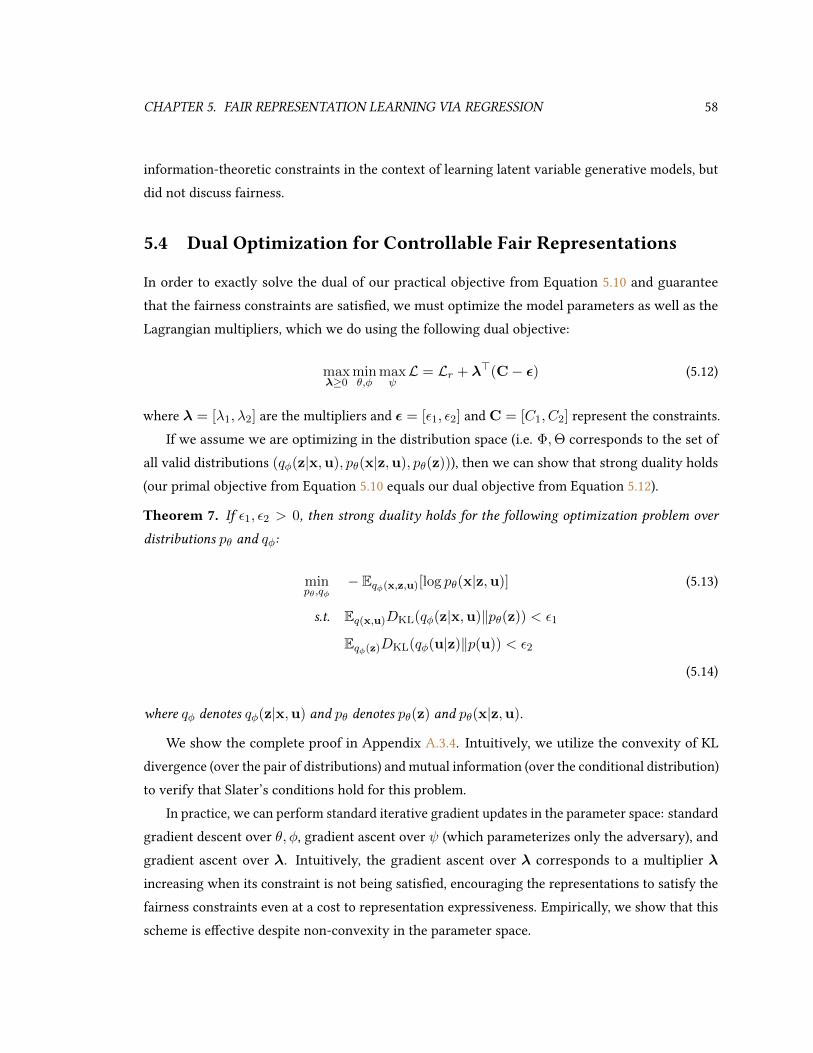
CHAPTER 5. FAIR REPRESENTATION LEARNING VIA REGRESSION 58
information-theoretic constraints in the context of learning latent variable generative models, butdid not discuss fairness.
5.4 Dual Optimization for Controllable Fair Representations
In order to exactly solve the dual of our practical objective from Equation 5.10 and guaranteethat the fairness constraints are satised, we must optimize the model parameters as well as theLagrangian multipliers, which we do using the following dual objective:
maxλ≥0
minθ,φ
maxψL = Lr + λ>(C− ε) (5.12)
where λ = [λ1, λ2] are the multipliers and ε = [ε1, ε2] and C = [C1, C2] represent the constraints.If we assume we are optimizing in the distribution space (i.e. Φ,Θ corresponds to the set of
all valid distributions (qφ(z|x,u), pθ(x|z,u), pθ(z))), then we can show that strong duality holds(our primal objective from Equation 5.10 equals our dual objective from Equation 5.12).
Theorem 7. If ε1, ε2 > 0, then strong duality holds for the following optimization problem over
distributions pθ and qφ:
minpθ,qφ
− Eqφ(x,z,u)[log pθ(x|z,u)] (5.13)
s.t. Eq(x,u)DKL(qφ(z|x,u)‖pθ(z)) < ε1
Eqφ(z)DKL(qφ(u|z)‖p(u)) < ε2
(5.14)
where qφ denotes qφ(z|x,u) and pθ denotes pθ(z) and pθ(x|z,u).
We show the complete proof in Appendix A.3.4. Intuitively, we utilize the convexity of KLdivergence (over the pair of distributions) and mutual information (over the conditional distribution)to verify that Slater’s conditions hold for this problem.
In practice, we can perform standard iterative gradient updates in the parameter space: standardgradient descent over θ, φ, gradient ascent over ψ (which parameterizes only the adversary), andgradient ascent over λ. Intuitively, the gradient ascent over λ corresponds to a multiplier λincreasing when its constraint is not being satised, encouraging the representations to satisfy thefairness constraints even at a cost to representation expressiveness. Empirically, we show that thisscheme is eective despite non-convexity in the parameter space.
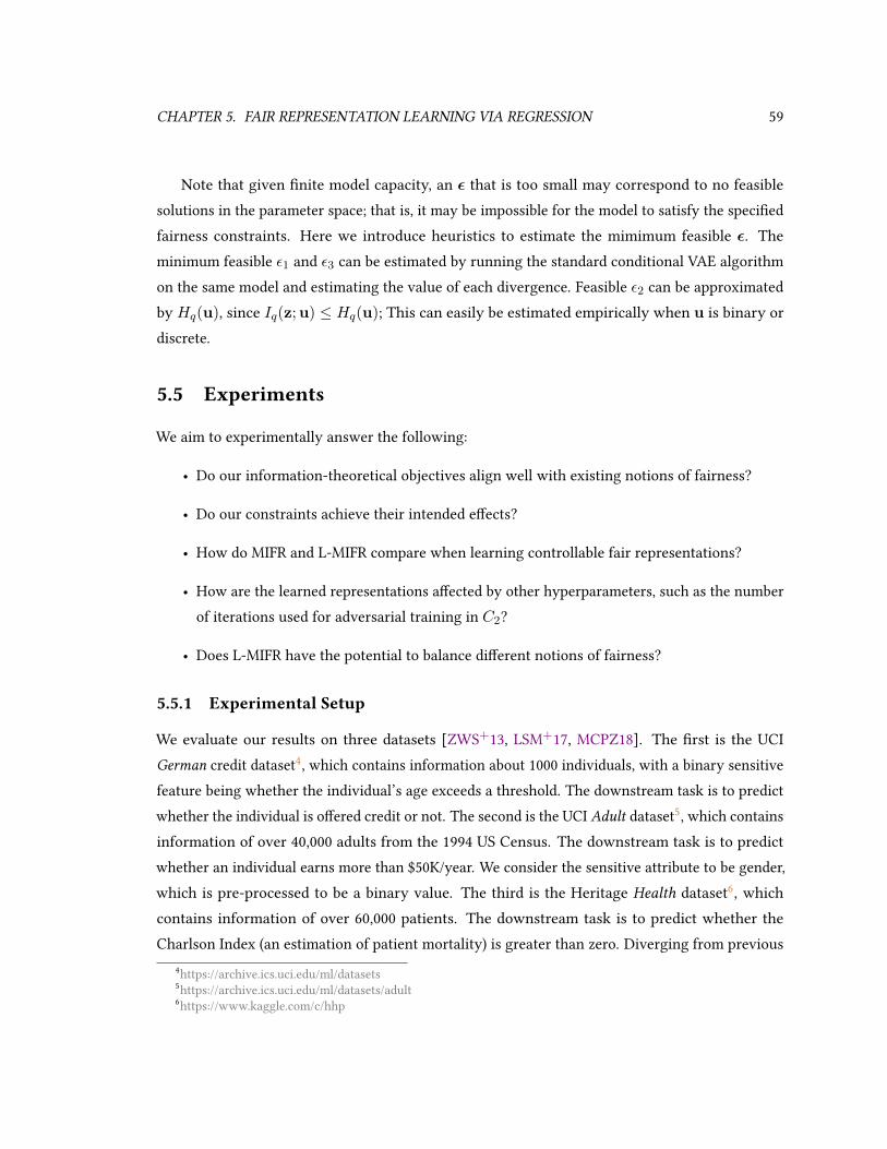
CHAPTER 5. FAIR REPRESENTATION LEARNING VIA REGRESSION 59
Note that given nite model capacity, an ε that is too small may correspond to no feasiblesolutions in the parameter space; that is, it may be impossible for the model to satisfy the speciedfairness constraints. Here we introduce heuristics to estimate the mimimum feasible ε. Theminimum feasible ε1 and ε3 can be estimated by running the standard conditional VAE algorithmon the same model and estimating the value of each divergence. Feasible ε2 can be approximatedby Hq(u), since Iq(z;u) ≤ Hq(u); This can easily be estimated empirically when u is binary ordiscrete.
5.5 Experiments
We aim to experimentally answer the following:
• Do our information-theoretical objectives align well with existing notions of fairness?
• Do our constraints achieve their intended eects?
• How do MIFR and L-MIFR compare when learning controllable fair representations?
• How are the learned representations aected by other hyperparameters, such as the numberof iterations used for adversarial training in C2?
• Does L-MIFR have the potential to balance dierent notions of fairness?
5.5.1 Experimental Setup
We evaluate our results on three datasets [ZWS+13, LSM+17, MCPZ18]. The rst is the UCIGerman credit dataset4, which contains information about 1000 individuals, with a binary sensitivefeature being whether the individual’s age exceeds a threshold. The downstream task is to predictwhether the individual is oered credit or not. The second is the UCI Adult dataset5, which containsinformation of over 40,000 adults from the 1994 US Census. The downstream task is to predictwhether an individual earns more than $50K/year. We consider the sensitive attribute to be gender,which is pre-processed to be a binary value. The third is the Heritage Health dataset6, whichcontains information of over 60,000 patients. The downstream task is to predict whether theCharlson Index (an estimation of patient mortality) is greater than zero. Diverging from previous
4https://archive.ics.uci.edu/ml/datasets5https://archive.ics.uci.edu/ml/datasets/adult6https://www.kaggle.com/c/hhp

CHAPTER 5. FAIR REPRESENTATION LEARNING VIA REGRESSION 60
work [MCPZ18], we consider sensitive attributes to be age and gender, where there are 9 possibleage values and 2 possible gender values; hence the sensitive attributes have 18 congurations. Thisprevents VFAE [LSL+15] and LAFTR [MCPZ18] from being applied, as both methods reply onsome statistical distance between two groups, which is not dened when there are 18 groups inquestion7.
We assume that the model does not have access to labels during training; instead, it supplies itsrepresentations to an unknown vendor’s classier, whose task is to achieve high prediction withlabels. We compare the performance of MIFR, the model with xed multipliers, and L-MIFR, themodel using the Lagrangian dual optimization method. We provide details of the experimentalsetup in Appendix B.3.1. Specically, we consider the simpler form for p(z) commonly used inVAEs, where p(z) is a xed prior; the use of other more exible parametrized forms of p(z), suchas normalizing ows [DSDB16, RM15] and autoregressive models [KSJ+16b, vdOKK16], is left asfuture work.
We estimate the mutual information values Iq(x; z|u) and Iq(u; z) on the test set using thefollowing equations:
Iq(x; z|u) = Eqφ(x,z,u)[log qφ(z|x,u)− log qφ(z|u)]
Iq(u; z) = Eqφ(x,z,u)[log qφ(u|z)− log q(u)]
where qφ(z|u) is estimated via kernel density estimation over samples from qφ(z|x,u) with(x,u) sampled from the training set. Kernel density estimates are reasonable since both z andu are low dimensional (for example, Adult considers a 10-dimension z for 40,000 individuals).However, computing qφ(z|u) requires a summation over the training set, so we only computethese mutual information quantities during evaluation. We include our implementations inhttps://github.com/ermongroup/lag-fairness.
5.5.2 Mutual Information, Prediction Accuracy, and Fairness
We investigate the relationship between mutual information and prediction performance by con-sidering area under the ROC curve (AUC) for prediction tasks. We also investigate the relationshipbetween mutual information and traditional fairness metrics by considering the ∆DP fairness met-ric in [MCPZ18], which compares the absolute expected dierence in classier outcomes betweentwo groups. ∆DP is only dened on two groups of classier outcomes, so it is not dened for
7∆DP is only dened for binary sensitive variables in [MCPZ18].

CHAPTER 5. FAIR REPRESENTATION LEARNING VIA REGRESSION 61
10 15 20 25Iq(x, z|u)
0.55
0.60
0.65
Test
AUC
0.0 0.2 0.4 0.6Iq(z, u)
0.0
0.1
0.2
Δ DP
PCA FeaturesLearned Features
German
2.5 5.0 7.5 10.0 12.5 15.0 17.5Iq(x, z|u)
0.60
0.65
0.70
Test
AUC
0.0 0.1 0.2 0.3Iq(z, u)
0.0
0.1
0.2
Δ DP
PCA FeaturesLearned Features
Adult
10 20 30 40Iq(x, z|u)
0.55
0.60
0.65
0.70
Test
AUC
Health
Figure 5.1: The relationship between mutual information and fairness related quantities. Each dotis the representations from an instance of MIFR with a dierent set of hyperparameters. Greenline represents features obtained via principle component analysis. Increased mutual informationbetween inputs and representations increase task performance (left) and unfairness (right). ForHealth we do not include ∆DP since it is not dened for more than two groups.

CHAPTER 5. FAIR REPRESENTATION LEARNING VIA REGRESSION 62
5.0 12.0 19.0 26.0ε1
5
10
15
20
25
C 1
0.1 0.2 0.3 0.4ε2
0.1
0.2
0.3
0.4
C 2
German
2.0 6.0 10.0 14.0ε1
5
10
15
C 1
0.02 0.05 0.1 0.15ε2
0.05
0.10
0.15
C 2
Adult
5.0 10.0 15.0 20.0ε1
5
10
15
20
C 1
0.1 0.2 0.3 0.4ε2
0.1
0.2
0.3
0.4
C 2
Health
Figure 5.2: Corresponding Ci values under dierent εi with L-MIFR. After εi is xed, we consider arange of values for the other constraint, leading to a distribution of Ci for each εi (hence the boxplot).

CHAPTER 5. FAIR REPRESENTATION LEARNING VIA REGRESSION 63
the Health dataset when considering the sensitive attributes to be “age and gender”, which has 18groups. We use logistic regression classiers for prediction tasks.
From the results results in Figure 5.1, we show that there are strong positive correlationsbetween Iq(x; z|u) and test AUC, and between Iq(z,u) and ∆DP ; increases in Iq(z,u) decreasefairness. We also include a baseline in Figure 5.1 where the features are obtained via the top-k principal components (where k is the dimension of z), which has slightly better AUC butsignicantly worse fairness as measured by ∆DP . Therefore, our information theoretic notions offairness/expressiveness align well with existing notions such as ∆DP /test AUC.
5.5.3 Controlling Representation Fairness with L-MIFR
Keeping all other constraint budgets xed, any increase in εi for an arbitrary constraint Ci impliesan increase in the unfairness budget; consequently, we are able to trade-o fairness for moreinformative representations when desired.
We demonstrate this empirically via an experiment where we note the Ci values correspondingto a range of budgets εi at a xed conguration of the other constraint budgets εj (j 6= i). FromFigure 5.2, Ci increases as εi increases, and Ci < εi holds under dierent values of the otherconstraints εj . This suggest that we can use εi to control Ci (our fairness criteria) of the learnedrepresentations.
We further show the changes in ∆DP (a traditional fairness criteria) values as we vary εi inFigure 5.3. In Adult, ∆DP clearly increases as εi increases; this is less obvious in German, as ∆DP
is already very low. These results suggest that the L-MIFR user can control the level of fairness ofthe representations quantitatively via ε.
5.5.4 Improving Representation Expressiveness with L-MIFR
Recall that our goal is to perform controlled fair representation learning, which requires us tolearn expressive representations subject to fairness constraints. We compare two approaches thatcould achieve this: 1) MIFR, which has to consider a range of Lagrange multipliers (e.g. from a gridsearch) to obtain solutions that satisfy the constraints; 2) L-MIFR, which nds feasible solutionsdirectly by optimizing the Lagrange multipliers.
We evaluate both methods on 4 sets of constraints by modifying the values of ε2 (which isthe tighter estimate of Iq(z;u)) while keeping ε1 xed, and we compare the expressiveness of thefeatures learned by the two methods in Figure 5.4. For MIFR, we perform a grid search running

CHAPTER 5. FAIR REPRESENTATION LEARNING VIA REGRESSION 64
5.0 12.0 19.0 26.0ε1
0.01
0.02
0.03
0.04Δ D
P
0.1 0.2 0.3 0.4ε2
0.01
0.02
0.03
0.04
Δ DP
German
2.0 6.0 10.0 14.0ε1
0.02
0.04
0.06
0.08
0.10
Δ DP
0.02 0.05 0.1 0.15ε2
0.04
0.06
0.08
Δ DP
Adult
Figure 5.3: ∆DP under dierent levels of ε with L-MIFR. ∆DP generally increases as ε increases.
52 = 25 congurations. In contrast, we run one instance of L-MIFR for each ε setting, which takesroughly the same time to run as one instance of MIFR (the only overhead is updating the two scalarvalues λ1 and λ2).
0.02 0.05 0.10 0.15ε2
11
12
13
14
I q(x,z|u)
Adult
MIFRL-MIFR
0.1 0.2 0.3 0.4ε2
19
20
21
22
23
I q(x,z|u)
HealthMIFRL-MIFR
Figure 5.4: Expressiveness vs. ε2. A larger feasible region (as measured by ε2) leads to moreexpressive representations (as measured by Iq(x, z|u)).
In terms of representation expressiveness, L-MIFR outperforms MIFR even though MIFR tookalmost 25x the computational resources. Therefore, L-MIFR is signicantly more computationallyecient than MIFR at learning controlled fair representation.

CHAPTER 5. FAIR REPRESENTATION LEARNING VIA REGRESSION 65
D =1 D =2 D =5 D =10
Adult Iq(x; z|u) 10.46 10.94 9.75 9.54Iq(z;u) 0.10 0.07 0.08 0.06
Health Iq(x; z|u) 16.60 16.47 16.65 16.75Iq(z;u) 0.17 0.17 0.22 0.28
Table 5.2: Expressiveness and fairness of the representations from L-MIFR under various D.
5.5.5 Ablation Studies
The C2 objective requires adversarial training, which involves iterative training of (θ, φ) withψ. We assess the sensitivity of the expressiveness and fairness of the learned representations tothe number of iterations D for ψ per iteration for (θ, φ). Following practices in [GAA+17] tohave more iterations for critic, we consider D = 1, 2, 5, 10, and use the same number of totaliterations for training.
In Table 5.2, we evaluate Iq(x; z|u) and Iq(z;u) obtained L-MIFR on Adult (ε2 = 0.10) andHealth (ε2 = 0.30). This suggests that the nal solution of the representations is not very sensitiveto D, although larger D seem to nd solutions that are closer to ε2.
5.5.6 Fair Representations under Multiple Notions
Finally, we demonstrate how L-MIFR could control multiple fairness constraints simultaneously,thereby nding representations that are reasonably fair when there are multiple fairness notionsbeing considered. We consider the Adult dataset, and describe the demographic parity, equalizedodds and equalized opportunity notions of fairness in terms of mutual information, which we denoteas IDP := Iq(z;u), IEO, IEOpp respectively (see details in Appendix B.3.3 about how IEO andIEOpp are derived).
For L-MIFR, we set ε1 = 10 and other ε values to 0.1. For MIFR, we consider a more ecientapproach than random grid search. We start by setting every λ = 0.1; then we multiply the λvalue for a particular constraint by 2 until the constraint is satised by MIFR; we nish when allthe constraints are satised8. We nd that this requires us to update the λ of IDP , IEO and IEOppfour times each (so corresponding λ = 1.6); this costs 12x the computational resources needed byL-MIFR.
8This allows MIFR to approach the feasible set from outside, so the solution it nds will generally have highexpressiveness.

CHAPTER 5. FAIR REPRESENTATION LEARNING VIA REGRESSION 66
Iq(x; z|u) C1 IDP IEO IEOpp
MIFR 9.34 9.39 0.09 0.10 0.07L-MIFR 9.94 9.95 0.08 0.09 0.04
Table 5.3: Learning one representation for multiple notions of fairness on Adult. L-MIFR learnsrepresentations that are better than MIFR on all the measurements instead of onlyC1. Here ε1 = 10for C1 and ε = 0.1 for other constraints.
We compare the representations learned by L-MIFR and MIFR in Figure 5.3. L-MIFR outperformsMIFR in terms of Iq(x; z|u), IDP , IEO and IEOpp, while only being slightly worse in terms of C1.Since ε1 = 10, the L-MIFR solution is still feasible. This demonstrates that even with a thoughtfullydesigned method for tuning λ, MIFR is still much inferior to L-MIFR in terms of computational costand representation expressiveness.
5.6 Discussion
In this chapter, we introduced an objective for learning controllable fair representations based onmutual information. This interpretation allows us to unify and explain existing work. In particular,we have shown that a range of existing approaches optimize an approximation to the Lagrangiandual of our objective with xed multipliers, xing the trade-o between fairness and expressiveness.We proposed a dual optimization method that allows us to achieve higher expressiveness whilesatisfying the user-specied limit on unfairness.
In future work, we are interested in formally and empirically extending this framework andthe corresponding dual optimization method to other notions of fairness. It is also valuable toinvestigate alternative approaches to training the adversary [GAA+17], the usage of more exiblep(z) [RM15], and alternative solutions to bounding Iq(z,u).

Part II
Generation via Supervised Learning
67

Chapter 6
Generation with ReweightedObjectives
Generative adversarial networks (GANs) variants approximately minimize divergences betweenthe model and the data distribution using a discriminator. Wasserstein GANs (WGANs) enjoysuperior empirical performance, however, unlike in f -GANs, the discriminator does not provide anestimate for the ratio between model and data densities, which is useful in applications such asinverse reinforcement learning.
In this chapter, we propose an new training objective where we additionally optimize overa set of importance weights over the generated samples. By suitably constraining the feasibleset of importance weights, we obtain a family of objectives which includes and generalizes theoriginal f -GAN and WGAN objectives. We show that a natural extension outperforms WGANswhile providing density ratios as in f -GAN, and demonstrate empirical success on distributionmodeling, density ratio estimation and image generation.
6.1 Introduction
Learning generative models to sample from complex, high-dimensional distributions is an importanttask in machine learning with many important applications, such as image generation [KW13],imitation learning [HE16] and representation learning [CDH+16]. Generative adversarial networks(GANs, [GPAM+14]) are likelihood-free deep generative models [ML16] based on nding the equi-librium of a two-player minimax game between a generator and a critic (discriminator). Assumingthe optimal critic is obtained, one can cast the GAN learning procedure as minimizing a discrepancy
68

CHAPTER 6. GENERATION WITH REWEIGHTED OBJECTIVES 69
measure between the distribution induced by the generator and the training data distribution.Various GAN learning procedures have been proposed for dierent discrepancy measures.
f -GANs [NCT16] minimize a variational approximation of the f -divergence between two distribu-tions [Csi64, NWJ08]. In this case, the critic acts as a density ratio estimator [USS+16, GE17], i.e.,it estimates if points are more likely to be generated by the data or the generator distribution. Thisincludes the original GAN approach [GPAM+14] which can be seen as minimizing a variationalapproximation to the Jensen-Shannon divergence. Knowledge of the density ratio between twodistributions can be used for importance sampling and in a range of practical applications such asmutual information estimation [DHFLM+18], o-policy policy evaluation [LLTZ18], and de-biasingof generative models [GSA+19].
Another family of GAN approaches are developed based on Integral Probability Metrics (IPMs,[Mül97]), where the critic (discriminator) is restricted to particular function families. For the familyof Lipschitz-1 functions, the IPM reduces to the Wasserstein-1 or earth mover’s distance [RTG00],which motivates the Wasserstein GAN (WGAN, [ACB17]) setting. Various approaches have beenapplied to enforce Lipschitzness, including weight clipping [ACB17], gradient penalty [GAA+17]and spectral normalization [MKKY18]. Despite its strong empirical success in image genera-tion [KALL17, BDS18], the learned critic cannot be interpreted as a density ratio estimator, whichlimits its usefulness for importance sampling or other GAN-related applications such as inversereinforcement learning [YSE19].
In this chapter, we address this problem via a generalized view of f -GANs and WGANs. Thegeneralized view introduces importance weights over the generated samples in the critic objective,allowing prioritization over the training of dierent samples. The algorithm designer can selectsuitable feasible sets to constrain the importance weights; we show that both f -GAN and WGANare special cases to this generalization when specic feasible sets are considered. We further discusscases that select alternative feasible sets where divergences other than f -divergence and IPMs canbe obtained.
To derive concrete algorithms, we turn to a case where the importance weights belong to theset of valid density ratios over the generated distribution. In certain cases, the optimal importanceweights can be obtained via closed-form solutions, bypassing the need to perform an additionalinner-loop optimization. We discuss one such approach, named KL-Wasserstein GAN (KL-WGAN),that is easy to implement from existing WGAN approaches, and is compatible with state-of-the-art GAN architectures. We evaluate KL-WGAN empirically on distribution modeling, densityestimation and image generation tasks. Empirical results demonstrate that KL-WGAN enjoys

CHAPTER 6. GENERATION WITH REWEIGHTED OBJECTIVES 70
superior quantitative performance compared to its WGAN counterparts on several benchmarks.
6.2 Preliminaries
Notations Let X denote a random variable with separable sample space X and let P(X ) denotethe set of all probability measures over the Borel σ-algebra on X . We use P , Q to denote probabiliymeasures, and P Q to denote P is absolutely continuous with respect to Q, i.e., the Radon-Nikodym derivative dP/ dQ exists. Under Q ∈ P(X ), the p-norm of a function r : X → R isdened as
‖r‖p :=
(∫|r(x)|pdQ(x)
)1/p
, (6.1)
with ‖r‖∞ = limp→∞‖r‖p. The set of locally p-integrable functions is dened as
Lp(Q) := r : X → R : ‖r‖p <∞, (6.2)
i.e. its norm with respect to Q is nite. We denote Lp≥0(Q) := r ∈ Lp(Q) : ∀x ∈ X , r(x) ≥ 0which considers non-negative functions in Lp(Q). The space of probability measures wrt. Q isdened as
∆(Q) := r ∈ L1≥0(Q) : ‖r‖1 = 1. (6.3)
For example, for any P Q, dP/ dQ ∈ ∆(Q) because∫
(dP/ dQ) dQ = 1. We dene 1 such that∀x ∈ X , 1(x) = 1, and dene im(·) and dom(·) as image and domain of a function respectively.
Integral Probability Metrics andWasserstein GANs For a xed class of real-valued boundedBorel measurable functions F on X , the integral probability metric (IPM) based on F and betweenP,Q ∈ P(X ) is dened as:
IPMF (P,Q) := supT∈F
∣∣∣∣∫ T (x) dP (x)−∫T (x) dQ(x)
∣∣∣∣ .If for all T ∈ F ,−T ∈ F then IPMF forms a metric over P(X ) [Mül97]; we assume this is alwaystrue for F in this paper (so we can remove the absolute values). In particular, if F is the set ofall bounded 1-Lipschitz functions with respect to the metric over X , then the corresponding IPM

CHAPTER 6. GENERATION WITH REWEIGHTED OBJECTIVES 71
becomes the Wasserstein distance between P and Q [Vil08]. This motivates the Wasserstein GANobjective [ACB17]:
minθ
maxφ
Ex∼Pdata[Tφ(x)]− Ex∼Qθ [Tφ(x)], (6.4)
where Tφ is regularized to be approximately k-Lipschitz for some k. Various approaches have beenapplied to enforce Lipschitzness of neural networks, including weight clipping [ACB17], gradientpenalty [GAA+17], and spetral normalization over the weights [MKKY18].
Despite its strong empirical performance, WGAN has two drawbacks. First, unlike f -GAN(Lemma 2), it does not naturally recover a density ratio estimator from the critic. Granted, theWGAN objective corresponds to an f -GAN one [SFG+09] when f(x) = 0 if x = 1 and f(x) = +∞otherwise, so that f∗(x) = x; however, we can no longer use Lemma 2 to recover density ratiosgiven an optimal critic T , because the derivative f ′(x) does not exist. Second, WGAN places thesame weight on the objective for each generated sample, which could be sub-optimal when thegenerated samples are of dierent qualities.
6.3 A Generalization of f-GANs and WGANs
In order to achieve the best of both worlds, we propose an alternative generalization to the criticobjectives to both f -GANs and WGANs. Consider the following functional:
`f (T, r;P,Q) := Ex∼Q[f(r(x))] + Ex∼P [T (x)]− Ex∼Q[r(x) · T (x)] (6.5)
which depends on the distributions P and Q, the critic function T : X → R, and an additionalfunction r : X → R. For conciseness, we remove the dependency on the argument x for T, r, P,Qin the remainder of the paper.
The function r : X → R here plays the role of “importance weights”, as they changes theweights to the critic objective over the generator samples. When r = dP/ dQ, the objective abovesimplies to EQ[f(dP/ dQ)] which is exactly the denition of the f -divergence between P and Q(Eq. 2.5).
To recover an objective over only the critic T , we minimize `f as a function of r over a suitablesetR ⊆ L∞≥0(Q), thus eliminating the dependence over r:
LRf (T ;P,Q) := infr∈R
`f (T, r;P,Q) (6.6)

CHAPTER 6. GENERATION WITH REWEIGHTED OBJECTIVES 72
We note that the minimization step is performed within a particular setR ⊆ L∞(Q), whichcan be selected by the algorithm designer. The choice of the setR naturally gives rise to dierentcritic objectives. As we demonstrate below (and in Figure 6.1), we can obtain critic objectives forf -GAN as well as WGANs as special cases via dierent choices ofR in LRf (T ;P,Q).
6.3.1 Recovering the f-GAN Critic Objective
First, we can recover the critic in the f -GAN objective by settingR = L∞≥0(Q), which is the set ofall non-negative functions in L∞(Q). Recall from Lemma 2 the f -GAN objective:
Df (P‖Q) = supT∈L∞(Q)
If (T ;P,Q) (6.7)
where If (T ;P,Q) := EP [T ] − EQ[f∗(T )] as dened in Lemma 2. The following propositionshows that whenR = L∞≥0(Q), we recover If = LRf .
Proposition 1. Assume that f is dierentiable at [0,∞). ∀P,Q ∈ P(X ) such that P Q, and
∀T ∈ F ⊆ L∞(Q) such that im(T ) ⊆ dom((f ′)−1),
If (T ;P,Q) = infr∈L∞≥0(Q)
`f (T, r;P,Q). (6.8)
where If (T ;P,Q) := EP [T ]− EQ[f∗(T )].
Proof. From Fenchel’s inequality we have for convex f : R → R, ∀T (x) ∈ R and ∀r(x) ≥ 0,f(r(x)) + f∗(T (x)) ≥ r(x)T (x) where equality holds when T (x) = f ′(r(x)). Taking theexpectation over Q, we have
EQ[f(r)]− EQ[rT ] ≥ −EQ[f∗(T )]; (6.9)
applying this to the denition of `f (T, r;P,Q), we have:
`f (T, r;P,Q) := EQ[f(r)] + EP [T ]− EQ[rT ]
≥ EP [T ]− EQ[f∗(T )] = If (T ;P,Q). (6.10)
where the inequality comes from Equation 6.9. The inequality becomes an equality when r(x) =
(f ′)−1(T (x)) for all x ∈ X . We note that such a case can be achieved, i.e., (f ′)−1(T ) ∈ L∞≥0(Q),because ∀x ∈ X , (f ′)−1(T (x)) ∈ dom(f) = [0,∞) from the assumption over im(T ). Therefore,

CHAPTER 6. GENERATION WITH REWEIGHTED OBJECTIVES 73
taking the inmum over r ∈ L∞≥0(Q), we have:
If (T ;P,Q) = infr∈L∞≥0(Q)
`f (T, r;P,Q), (6.11)
which completes the proof.
6.3.2 Recovering the WGAN Critic Objective
Next, we recover the WGAN critic objective (IPM) by setting R = 1, where 1(x) = 1 is aconstant function. First, we can equivalently rewrite the denition of an IPM using the followingnotation:
IPMF (P,Q) = supT∈F
IW (T ;P,Q) (6.12)
where IW represents the critic objective. We show that IW = LRf whenR = 1 as follows.
Proposition 2. ∀P,Q ∈ P(X ) such that P Q, and ∀T ∈ F ⊆ L∞(Q):
IW (T ;P,Q) = infr∈1
`f (T, r;P,Q) (6.13)
where IW (T ;P,Q) := EP [T ]− EQ[T ].
Proof. As 1 has only one element, the inmum is:
`f (T,1;P,Q) = EQ[f(1)] + EP [T ]− EQ[T ] = IW (T ;P,Q) (6.14)
where we used f(1) = 0 for the second equality.
The above propositions show that LRf generalizes both f -GAN and WGANs critic objectivesby settingR = L∞≥0(Q) andR = 1 respectively.
6.3.3 Extensions to Alternative Constraints
The generalization with LRf allows us to introduce new objectives when we consider alternativechoices for the constraint setR. We consider setsR such that 1 ⊆ R ⊆ L∞≥0(Q). The followingproposition shows for some xed T , the corresponding objective withR is bounded between thef -GAN objective (whereR = L∞≥0(Q)) and the WGAN objective (whereR = 1).

CHAPTER 6. GENERATION WITH REWEIGHTED OBJECTIVES 74
Figure 6.1: High-level idea of f -WGAN. (Left) Minimization over dierentR inLRf gives dierentcritic objectives. Minimizing overL∞≥0(Q) recovers f -GAN (blue set), minimizing over 1 recoversWGAN (orange set), and minimizing over ∆(Q) recovers f -WGAN (green set). (Right) Naturally,as we consider smaller setsR to minimize over, the critic objective becomes larger for the same T .
Proposition 3. ∀P,Q ∈ P(X ) such that P Q, ∀T ∈ L∞(Q) such that im(T ) ⊆ dom((f ′)−1),
and ∀R ⊆ L∞≥0(Q) such that 1 ⊆ R we have:
If (T ;P,Q) ≤ LRf (T ;P,Q) ≤ IW (T ;P,Q). (6.15)
Proof. In Appendix A.4.
We visualize this in Figure 6.1. Selecting the setR allows us to control the critic objective ina more exible manner, interpolating between the f -GAN critic and the IPM critic objective andnding suitable trade-os. Moreover, if we additionally take the supremum of LRf (T ;P,Q) over T ,the result will be bounded between the supremum of If over T (corresponding to the f -divergence)and the supremum of IW over T , as stated in the following theorem.
Theorem 8. For 1 ⊆ R ⊆ L∞≥0(Q), dene
Df,R(P‖Q) := supT∈FLRf (T ;P,Q) (6.16)
where F := T : X → dom((f ′)−1), T ∈ L∞(Q). Then
Df (P‖Q) ≤ Df,R(P‖Q) ≤ supT∈F
IW (T ;P,Q). (6.17)
Proof. In Appendix A.4.
A natural corollary is that Df,R denes a divergence between two distributions.

CHAPTER 6. GENERATION WITH REWEIGHTED OBJECTIVES 75
Corollary 5. Df,R(P‖Q) denes a divergence between P and Q: Df,R(P‖Q) ≥ 0 for all P,Q ∈P(X ), and Df,R(P‖Q) = 0 if and only if P = Q.
This allows us to interpret the corresponding GAN algorithm as variational minimization of acertain divergence bounded between the corresponding f -divergence and IPM.
6.4 Practical f-Wasserstein GANs
As a concrete example, we consider the setR = ∆(Q), which is the set of all valid density ratiosover Q. We note that 1 ⊂ ∆(Q) ⊂ L∞≥0(Q) (see Figure 6.1), so the corresponding objective isa divergence (from Corollary 5). We can then consider the variational divergence minimizationobjective over L∆(Q)
f (T ;P,Q):
infQ∈P(X )
supT∈F
infr∈∆(Q)
`f (T, r;P,Q), (6.18)
We name this the “f -Wasserstein GAN” (f -WGAN) objective, since it provides an interpolationbetween f -GAN and Wasserstein GANs while recovering a density ratio estimate between twodistributions.
6.4.1 KL-Wasserstein GANs
For the f -WGAN objective in equation 6.18, the trivial algorithm would have to perform iterativeupdates to three quantitiesQ, T and r, which involves three nested optimizations. While this seemsimpractical, we show that for certain choices of f -divergences, we can obtain closed-form solutionsfor the optimal r ∈ ∆(Q) in the innermost minimization; this bypasses the need to perform aninner-loop optimization over r ∈ ∆(Q), as we can simply assign the optimal solution from theclose-form expression.
Theorem 9. Let f(u) = u log u and F a set of real-valued bounded measurable functions on X . Forany xed choice of P,Q, and T ∈ F , we have
arg minr∈∆(Q)
EQ[f(r)] + EP [T ]− EQ[r · T ] =eT
EQ[eT ](6.19)
Proof. In Appendix A.4.

CHAPTER 6. GENERATION WITH REWEIGHTED OBJECTIVES 76
The above theorem shows that if the f -divergence of interest is the KL divergence, we candirectly obtain the optimal r ∈ ∆(Q) using equation 6.19 for any xed critic T . Then, we canapply this r to the f -WGAN objective, and perform gradient descent updates on Q and T only.Avoiding the optimization procedure over r allows us to propose practical algorithms that aresimilar to existing WGAN procedures. In Appendix B.4.2, we show a similar argument with χ2-divergence, another f -divergence admitting a closed-form solution, and discuss its connectionswith the χ2-GAN approach [TCH+18].
6.4.2 Implementation Details
In Algorithm 1, we describe KL-Wasserstein GAN (KL-WGAN), a practical algorithm motivatedby the f -WGAN objectives based on the observations in Theorem 9. We note that r0 correspondsto selecting the optimal value for r from Theorem 9; once r0 is selected, we ignore the eect ofEQ[f(r0)] to the objective and optimize the networks with the remaining terms, which correspondsto weighting the generated samples with r0; the critic will be updated as if the generated samples arereweighted. In particular,∇φ(D0−D1) corresponds to the critic gradient (T , which is parameterizedby φ) and∇θD1 corresponds to the generator gradient (Q, parameterized by θ).
In terms of implementation, the only dierences between KL-WGAN and WGAN are betweenlines 8 and 11, where WGAN will assign r0(x) = 1 for all x ∼ Qm. In contrast, KL-WGAN“importance weights” the samples using the critic, in the sense that it will assign higher weightsto samples that have large Tφ(x) and lower weights to samples that have low Tφ(x). This willencourage the generator Qθ(x) to put more emphasis on samples that have high critic scores. It isrelatively easy to implement the KL-WGAN algorithm from an existing WGAN implementation, aswe only need to modify the loss function. We present an implementation of KL-WGAN losses (inPyTorch) in Appendix B.4.1.
While the mini-batch estimation for r0(x) provides a biased estimate to the optimal r ∈ ∆(Q)
(which according to Theorem 9 is eTθ(x)/EQ[eTθ(x)], i.e., normalized with respect to Q instead ofover a minibatch of m samples as done in line 8), we found that this does not aect performancesignicantly. We further note that computing r0(x) does not require additional network evaluations,so the computational cost for each iteration is nearly identical between WGAN and KL-WGAN.
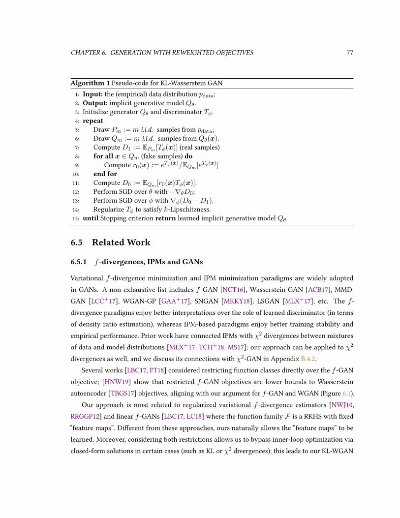
CHAPTER 6. GENERATION WITH REWEIGHTED OBJECTIVES 77
Algorithm 1 Pseudo-code for KL-Wasserstein GAN1: Input: the (empirical) data distribution pdata;2: Output: implicit generative model Qθ .3: Initialize generator Qθ and discriminator Tφ.4: repeat5: Draw Pm := m i.i.d. samples from pdata;6: Draw Qm := m i.i.d. samples from Qθ(x).7: Compute D1 := EPm [Tφ(x)] (real samples)8: for all x ∈ Qm (fake samples) do9: Compute r0(x) := eTφ(x)/EQm [eTφ(x)]
10: end for11: Compute D0 := EQm [r0(x)Tφ(x)].12: Perform SGD over θ with −∇θD0;13: Perform SGD over φ with∇φ(D0 −D1).14: Regularize Tφ to satisfy k-Lipschitzness.15: until Stopping criterion return learned implicit generative model Qθ .
6.5 Related Work
6.5.1 f-divergences, IPMs and GANs
Variational f -divergence minimization and IPM minimization paradigms are widely adoptedin GANs. A non-exhaustive list includes f -GAN [NCT16], Wasserstein GAN [ACB17], MMD-GAN [LCC+17], WGAN-GP [GAA+17], SNGAN [MKKY18], LSGAN [MLX+17], etc. The f -divergence paradigms enjoy better interpretations over the role of learned discriminator (in termsof density ratio estimation), whereas IPM-based paradigms enjoy better training stability andempirical performance. Prior work have connected IPMs with χ2 divergences between mixturesof data and model distributions [MLX+17, TCH+18, MS17]; our approach can be applied to χ2
divergences as well, and we discuss its connections with χ2-GAN in Appendix B.4.2.Several works [LBC17, FT18] considered restricting function classes directly over the f -GAN
objective; [HNW19] show that restricted f -GAN objectives are lower bounds to Wassersteinautoencoder [TBGS17] objectives, aligning with our argument for f -GAN and WGAN (Figure 6.1).
Our approach is most related to regularized variational f -divergence estimators [NWJ10,RRGGP12] and linear f -GANs [LBC17, LC18] where the function family F is a RKHS with xed“feature maps”. Dierent from these approaches, ours naturally allows the “feature maps” to belearned. Moreover, considering both restrictions allows us to bypass inner-loop optimization viaclosed-form solutions in certain cases (such as KL or χ2 divergences); this leads to our KL-WGAN

CHAPTER 6. GENERATION WITH REWEIGHTED OBJECTIVES 78
approach which is easy to implement from existing WGAN implementations, and also have similarcomputational cost per iteration.
6.5.2 Reweighting of Generated Samples
The learned discriminators in GANs can further be used to perform reweighting over the generatedsamples [TCH+18]; these include rejection sampling [AOD+18], importance sampling [GSA+19,TCH+18], and Markov chain monte carlo [THF+18]. These approaches can only be performedafter training has nished, unlike our KL-WGAN case where discriminator-based reweighting areperformed during training.
Moreover, prior reweighting approaches assume that the discriminator learns to approximatesome (xed) function of the density ratio dpdata/ dQθ, which does not apply directly to generalIPM-based GAN objectives (such as WGAN); in KL-WGAN, we interpret the discriminator outputsas (un-normalized, regularized) log density ratios, introducing the density ratio interpretation tothe IPM paradigm. We note that post-training discriminator-based reweighting can also be appliedto our approach, and is orthogonal to our contributions; we leave this as future work.
Table 6.1: Negative Log-likelihood (NLL) and Maximum mean discrepancy (MMD, multiplied by103) results on six 2-d synthetic datasets. Lower is better. W denotes the original WGAN objective,and KL-W denotes the proposed KL-WGAN objective.
Metric GAN MoG Banana Rings Square Cosine Funnel
NLL W 2.65± 0.00 3.61± 0.02 4.25± 0.01 3.73± 0.01 3.98± 0.00 3.60± 0.01KL-W 2.54± 0.00 3.57± 0.00 4.25± 0.00 3.72± 0.00 4.00± 0.01 3.57± 0.00
MMD W 25.45± 7.78 3.33± 0.59 2.05± 0.47 2.42± 0.24 1.24± 0.40 1.71± 0.65KL-W 6.51± 3.16 1.45± 0.12 1.20± 0.10 1.10± 0.23 1.33± 0.23 1.08± 0.23
6.6 Experiments
We release code for our experiments in https://github.com/ermongroup/f-wgan.
6.6.1 Synthetic and UCI Benchmark Datasets
We rst demonstrate the eectiveness of KL-WGAN on synthetic and UCI benchmark datasets [AN07]considered in [WSSG18]. The 2-d synthetic datasets include Mixture of Gaussians (MoG), Banana,Ring, Square, Cosine and Funnel; these datasets cover dierent modalities and geometries. We use

CHAPTER 6. GENERATION WITH REWEIGHTED OBJECTIVES 79
Figure 6.2: KL-WGAN samples on 2d distributions. Histograms of samples from the datadistribution (top), WGAN (middle) and our KL-WGAN (bottom).
Figure 6.3: Estimating density ratios with KL-WGAN. The rst column contains the samplesused for training, the second column is the ground truth density of P , the third and fourth columnsare the density of Q times the estimated density ratios from original f -GAN (third column) andour KL-WGAN (fourth column).
RedWine, WhiteWine and Parkinsons from the UCI datasets. We use the same SNGAN [MKKY18]arhictetures for WGAN and KL-WGANs, which uses spectral normalization to enforce Lipschitzness(detailed in Appendix B.4.3).
After training, we draw 5,000 samples from the generator and then evaluate two metricsover a xed validation set. One is the negative log-likelihood (NLL) of the validation sampleson a kernel density estimator tted over the generated samples; the other is the maximum meandiscrepancy (MMD, [BGR+06]) between the generated samples and validation samples. To ensurea fair comparison, we use identical kernel bandwidths for all cases.
Distribution modeling We report the mean and standard error for the NLL and MMD resultsin Tables 6.1 and 6.2 (with 5 random seeds in each case) for the synthetic datasets and UCI datasets

CHAPTER 6. GENERATION WITH REWEIGHTED OBJECTIVES 80
Table 6.2: Negative Log-likelihood (NLL, top two rows) and Maximum mean discrepancy (MMD,multiplied by 103, bottom two rows) results on real-world datasets. Lower is better for bothevaluation metrics. W denotes the original WGAN objective, and KL denotes the proposed KL-WGAN objective.
RedWine WhiteWine Parkinsons
W 14.55± 0.04 14.12± 0.02 20.24± 0.08KL 14.41± 0.03 14.08± 0.02 20.16± 0.05
W 2.61± 0.37 1.32± 0.10 1.30± 0.09KL 2.55± 0.11 1.23± 0.17 0.84± 0.04
Figure 6.4: Estimated divergencewithKL-WGAN.The results are shown with respect to trainingepochs (smoothed with a window of 10).
respectively. The results demonstrate that our KL-WGAN approach outperforms its WGAN coun-terpart on all but the Cosine dataset. From the histograms of samples in Figure 6.2, we can visuallyobserve where our KL-WGAN performs signicantly better than WGAN. For example, WGAN failsto place enough probability mass in the center of the Gaussians in MoG and fails to learn a propersquare in Square, unlike our KL-WGAN approaches.
Density ratio estimation We demonstrate that adding the constraint r ∈ ∆(Q) leads to eectivedensity ratio estimators. We consider measuring the density ratio from synthetic datasets, andcompare them with the original f -GAN with KL divergence. We evaluate the density ratio estimationquality by multiplying dQ with the estimated density ratios, and compare that with the density ofP ; ideally the two quantities should be identical. We demonstrate empirical results in Figure 6.3,where we plot the samples used for training, the ground truth density of P and the two estimatesgiven by two methods. In terms of estimating density ratios, our proposed approach is comparableto the f -GAN one.

CHAPTER 6. GENERATION WITH REWEIGHTED OBJECTIVES 81
Table 6.3: Inception and FID scores for CIFAR10 image generation. We list compar-isons with results reported by WGAN-GP [GAA+17], Fisher GAN [MS17], χ2 GAN [TCH+18],MoLM [RMRV18], SNGAN [MKKY18], NCSN [SE19c], BigGAN [BDS18] and Sphere GAN [PK19].(*) denotes our experiments with the PyTorch BigGAN implementation.
Method Inception score FID score
CIFAR10 Unconditional
WGAN-GP 7.86± .07 -Fisher GAN 7.90± .05 -MoLM 7.90± .10 18.9SNGAN 8.22± .05 21.7Sphere GAN 8.39± .08 17.1NCSN 8.91 25.32
BigGAN* 8.60± .10 16.38KL-BigGAN* 8.66± .09 15.23
CIFAR10 Conditional
Fisher GAN 8.16± .12 -WGAN-GP 8.42± .10 -χ2-GAN 8.44± .10 -SNGAN 8.60± .08 17.5BigGAN 9.22 14.73
BigGAN* 9.08± .11 9.51KL-BigGAN* 9.20± .09 9.17
Stability of critic objectives For the MoG, Square and Cosine datasets, we further show theestimated divergences over a batch of 256 samples in Figure 6.4, where WGAN uses IW and KL-WGAN uses the proposed L∆(Q)
f . While both estimated divergences decrease over the course oftraining, our KL-WGAN divergence is more stable on all three cases. In addition, we evaluate thenumber of occurrences when a negative estimate of the divergences was produced for an epoch(which contradicts the fact that divergences should be non-negative); over 500 batches, WGAN has46, 181 and 55 occurrences on MoG, Square and Cosine respectively, while KL-WGAN only has 29,100 and 7 occurrences. This suggests that the proposed objective is easier to estimate and optimize,and is more stable across dierent iterations.

CHAPTER 6. GENERATION WITH REWEIGHTED OBJECTIVES 82
Table 6.4: FID scores for CelebA image generation. The mean and standard deviation areobtained from 4 instances trained with dierent random seeds.
Method Image Size FID score
BigGAN64× 64
18.07± 0.47KL-BigGAN 17.70± 0.32
6.6.2 Image Generation
We further evaluate our KL-WGAN’s practical on image generation tasks on CIFAR10 and CelebAdatasets. Our experiments are based on the BigGAN [BDS18] PyTorch implementation. We use asmaller network than the one reported in [BDS18] (implemented on TensorFlow), using the defaultarchitecture in the PyTorch implementation.
We compare training a BigGAN network with its original objective and training same networkwith our proposed KL-WGAN algorithm, where we add steps 8 to 11 in Algorithm 1. In addition,we also experimented with the original f -GAN with KL divergence; this failed to train properlydue to numerical issues where exponents of very large critic values gives innity values in theobjective.
We report two common benchmarks for image generation, Inception scores [SGZ+16] andFréchet Inception Distance (FID) [HRU+17] 1 in Table 6.3 (CIFAR10) and Table 6.4 (CelebA). We donot report inception score on CelebA since the real dataset only has a score of less than 3, so thescore is not very indicative of generation performance [HRU+17]. We show generated samplesfrom the model in Appendix B.4.4.
Despite the strong performance of BigGAN, our method is able to consistently achieve superiorinception scores and FID scores consistently on all the datasets and across dierent random seeds.This demonstrates that the KL-WGAN algorithm is practically useful, and can serve as a viabledrop-in replacement for the existing WGAN objective even on state-of-the-art GAN models, suchas BigGAN.
6.7 Discussion
In this chapter, we introduce a generalization of f -GANs and WGANs based on optimizing a(regularized) objective over importance weighted samples. This perspective allows us to recover
1Based on https://github.com/mseitzer/pytorch-d

CHAPTER 6. GENERATION WITH REWEIGHTED OBJECTIVES 83
both f -GANs and WGANs when dierent sets to optimize for the importance weights are considered.In addition, we show that this generalization leads to alternative practical objectives for trainingGANs and demonstrate its eectiveness on several dierent applications, such as distributionmodeling, density ratio estimation and image generation. The proposed method only requires asmall change in the original training algorithm and is easy to implement in practice.
In future work, we are interested in considering other constraints that could lead to alternativeobjectives and/or inequalities and their practical performances. It would also be interesting toinvestigate the KL-WGAN approaches on high-dimensional density ratio estimation tasks suchas o-policy policy evaluation, inverse reinforcement learning and contrastive representationlearning.

Chapter 7
Generation with Negative DataAugmentation
In the previous chapter, we discussed how we can incorporate reweighting to the supervisedlearning objective and improve GAN training. In this chapter, we consider another improvementthat introduces certain data augmentations to the binary classication objective. Similar to tradi-tional data augmentations in supervised learning, this allows us to improve generative modelingperformance that cannot be achieved by the objective function alone.
Data augmentation is often used to enlarge datasets with synthetic samples generated inaccordance with the underlying data distribution. To enable a wider range of augmentations, weexplore negative data augmentation strategies (NDA) that intentionally create out-of-distributionsamples. We show that such negative out-of-distribution samples provide information on thesupport of the data distribution, and can be leveraged for generative modeling and representationlearning.
We introduce a new GAN training objective where we use NDA as an additional sourceof synthetic data for the discriminator. We prove that under suitable conditions, optimizing theresulting objective still recovers the true data distribution but can directly bias the generator towardsavoiding samples that lack the desired structure. Empirically, models trained with our methodachieve improved conditional/unconditional image generation along with improved anomalydetection capabilities. Further, we incorporate the same negative data augmentation strategy in acontrastive learning framework for self-supervised representation learning on images and videos,achieving improved performance on downstream image classication, object detection, and actionrecognition tasks. These results suggest that prior knowledge on what does not constitute valid
84

CHAPTER 7. GENERATION WITH NEGATIVE DATA AUGMENTATION 85
data is an eective form of weak supervision across a range of unsupervised learning tasks.This chapter is based on [SKS+21]. Abhishek Sinha and Ayush Kumar contributed to the
contents of this chapter. My contributions include providing the theory and initial code for theGAN and the contrastive learning setups.
7.1 Introduction
Data augmentation strategies for synthesizing new data in a way that is consistent with an under-lying task are extremely eective in both supervised and unsupervised learning [vdOLV18, ZIE16,NF16, ARV19]. Because they operate at the level of samples, they can be combined with mostlearning algorithms. They allow for the incorporation of prior knowledge (inductive bias) aboutproperties of typical samples from the underlying data distribution [JWAAN18, ASE17], e.g., byleveraging invariances to produce additional “positive” examples of how a task should be solved.
To enable users to specify an even wider range of inductive biases, we propose to leveragean alternative and complementary source of prior knowledge that species how a task shouldnot be solved. We formalize this intuition by assuming access to a way of generating samplesthat are guaranteed to be out-of-support for the data distribution, which we call a Negative Data
Augmentation (NDA). Intuitively, negative out-of-distribution (OOD) samples can be leveraged as auseful inductive bias because they provide information about the support of the data distributionto be learned by the model. For example, in a density estimation problem we can bias the model toavoid putting any probability mass in regions which we know a-priori should have zero probability.This can be an eective prior if the negative samples cover a suciently large area. The bestNDA candidates are ones that expose common pitfalls of existing models, such as prioritizing localstructure over global structure [GRM+18]; this motivates us to consider known transformationsfrom the literature that intentionally destroy the spatial coherence of an image [NF16, DT17,YHO+19], such as Jigsaw transforms.
Building on this intuition, we introduce a new GAN training objective where we use NDAas an additional source of fake data for the discriminator as shown in Fig. 7.1. Theoretically, wecan show that if the NDA assumption is valid, optimizing this objective will still recover the datadistribution in the limit of innite data. However, in the nite data regime, there is a need togeneralize beyond the empirical distribution [ZRY+18]. By explicitly providing the discriminatorwith samples we want to avoid, we are able to bias the generator towards avoiding undesirablesamples thus improving generation quality.
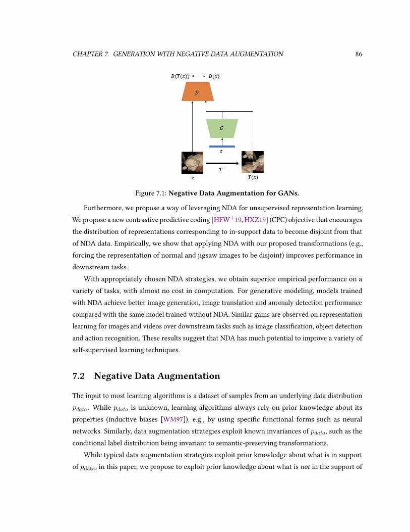
CHAPTER 7. GENERATION WITH NEGATIVE DATA AUGMENTATION 86
Figure 7.1: Negative Data Augmentation for GANs.
Furthermore, we propose a way of leveraging NDA for unsupervised representation learning.We propose a new contrastive predictive coding [HFW+19, HXZ19] (CPC) objective that encouragesthe distribution of representations corresponding to in-support data to become disjoint from thatof NDA data. Empirically, we show that applying NDA with our proposed transformations (e.g.,forcing the representation of normal and jigsaw images to be disjoint) improves performance indownstream tasks.
With appropriately chosen NDA strategies, we obtain superior empirical performance on avariety of tasks, with almost no cost in computation. For generative modeling, models trainedwith NDA achieve better image generation, image translation and anomaly detection performancecompared with the same model trained without NDA. Similar gains are observed on representationlearning for images and videos over downstream tasks such as image classication, object detectionand action recognition. These results suggest that NDA has much potential to improve a variety ofself-supervised learning techniques.
7.2 Negative Data Augmentation
The input to most learning algorithms is a dataset of samples from an underlying data distributionpdata. While pdata is unknown, learning algorithms always rely on prior knowledge about itsproperties (inductive biases [WM97]), e.g., by using specic functional forms such as neuralnetworks. Similarly, data augmentation strategies exploit known invariances of pdata, such as theconditional label distribution being invariant to semantic-preserving transformations.
While typical data augmentation strategies exploit prior knowledge about what is in supportof pdata, in this paper, we propose to exploit prior knowledge about what is not in the support of

CHAPTER 7. GENERATION WITH NEGATIVE DATA AUGMENTATION 87
pdata. This information is often available for common data modalities (e.g., natural images andvideos) and is under-exploited by existing approaches. Specically, we assume: (1) there existsan alternative distribution p such that its support is disjoint from that of pdata; and (2) access to aprocedure to eciently sample from p. We emphasize p need not be explicitly dened (e.g., throughan explicit density) – it may be implicitly dened by a dataset or by a procedure that transformssamples from pdata into ones from p by suitably altering their structure.
Figure 7.2: Negative augmentations produce out-of-distribution samples. Samples by nega-tive augmentations lack the typical structure of natural images, and can be used to inform a modelon what it should not learn.
Analogous to typical data augmentations, NDA strategies are by denition domain and taskspecic. In this paper, we focus on natural images and videos, and leave the application to otherdomains (such as natural language processing) as future work. How do we select a good NDAstrategy? According to the manifold hypothesis [FMN16], natural images lie on low-dimensionalmanifolds: pdata is supported on a low-dimensional manifold of the ambient (pixel) space. Thissuggests that many negative data augmentation strategies exist. Indeed, sampling random noise isin most cases a valid NDA. However, while this prior is generic, it is not very informative, and thisNDA will likely be ineective for most learning problems. Intuitively, NDA is informative if itssupport is close (in a suitable metric) to that of pdata, while being disjoint. These negative sampleswill provide information on the “boundary” of the support of pdata, which we will show is helpfulin several learning problems. In most of our tasks, the images are processed by convolutionalneural networks (CNNs) that are good at processing local features but not necessarily globalfeatures [GRM+18]. Therefore, we may consider NDA examples to be ones that preserve localfeatures (“informative”) and break global features, so that it forces the CNNs to learn global features(by realizing NDAs are dierent from real data).
Leveraging this intuition, we show several image transformations from the literature that can beviewed as generic NDAs over natural images in Figure 7.2, that we will use for generative modelingand representation learning in the following sections. Details about these transformations can befound in Appendix B.5.2.

CHAPTER 7. GENERATION WITH NEGATIVE DATA AUGMENTATION 88
7.3 NDA for Generative Adversarial Networks
Figure 7.3: Schematic overview of our NDA framework. Left: In the absence of NDA, thesupport of a generative modelPθ (blue oval) learned from samples (green dots) may “over-generalize”and include samples from P1 or P2. Right: With NDA, the learned distribution Pθ becomes disjointfrom NDA distributions P1 and P2, thus pushing Pθ closer to the true data distribution pdata (greenoval). As long as the prior is consistent, i.e. the supports of P1 and P2 are truly disjoint from pdata,the best t distribution in the innite data regime does not change.
In GANs, we are interested in learning a generative model Gθ from samples drawn from somedata distribution pdata [GPAM+14]. GANs use a binary classier, the so-called discriminatorDφ, todistinguish real data from generated (fake) samples. The generator Gθ is trained via the followingmini-max objective that performs variational Jensen-Shannon divergence minimization:
minGθ∈P(X )
maxDφ
LJS(Gθ, Dφ) where (7.1)
LJS(Gθ, Dφ) = Ex∼pdata [log(Dφ(x))] + Ex∼Gθ [log(1−Dφ(x))] (7.2)
This is a special case to the more general variational f -divergence minimization objective [NCT16].The optimal Dφ for any Gθ is (pdata/Gθ)/(1 + pdata/Gθ), so the discriminator can serve as adensity ratio estimator between pdata and Gθ .
With suciently expressive models and innite capacity, Gθ will match pdata. In practice,however, we have access to nite datasets and limited model capacity. This means that the generatorneeds to generalize beyond the empirical distribution, which is challenging because the numberof possible discrete distributions scale doubly exponentially w.r.t. to the data dimension. Hence,as studied in [ZRY+18], the role of the inductive bias is critical. For example, [ZRY+18] reportthat when trained on images containing 2 objects only, GANs and other generative models cansometimes “generalize” by generating images with 1 or 3 objects (which were never seen in the

CHAPTER 7. GENERATION WITH NEGATIVE DATA AUGMENTATION 89
training set). The generalization behavior – which may or may not be desirable – is determinedby factors such as network architectures, hyperparameters, etc., and is dicult to characterizeanalytically.
Here we propose to bias the learning process by directly specifying what the generator shouldnot generate through NDA. We consider an adversarial game based on the following objective:
minGθ∈P(X )
maxDφ
LJS(λGθ + (1− λ)P ,Dφ) (7.3)
where the negative samples are generated from a mixture of Gθ (the generator distribution) and P(the NDA distribution); the mixture weights are controlled by the hyperparameter λ. Intuitively,this can help addresses the above “over-generalization” issue, as we can directly provide supervisionon what should not be generated and thus guide the support of Gθ (see Figure 7.3) . For instance,in the object count example above, we can empirically prevent the model from generating imageswith an undesired number of objects (see Appendix Section A for experimental results on this task).
In addition, the introduction of NDA samples will not aect the solution of the original GANobjective in the limit. In the following theorem, we show that given innite training data andinnite capacity discriminators and generators, using NDA will not aect the optimal solution tothe generator, i.e. the generator will still recover the true data distribution.
Theorem 10. Let P ∈ P(X ) be any distribution over X with disjoint support than pdata, i.e.,
such that supp(pdata) ∩ supp(P ) = ∅. Let Dφ : X → R be the set of all discriminators over X ,f : R≥0 → R be a convex, semi-continuous function such that f(1) = 0, f? be the convex conjugate
of f , f ′ its derivative, and Gθ be a distribution with sample space X . Then ∀λ ∈ (0, 1], we have:
arg minGθ∈P(X )
maxDφ:X→R
Lf (Gθ, Dφ) = arg minGθ∈P(X )
maxDφ:X→R
Lf (λGθ + (1− λ)P ,Dφ) = pdata (7.4)
where Lf (Q,Dφ) = Ex∼pdata [Dφ(x)] − Ex∼Q[f?(Dφ(x))] is the objective for f -GAN [NCT16].
However, the optimal discriminators are dierent for the two objectives:
arg maxDφ:X→R
Lf (Gθ, Dφ) = f ′(pdata/Gθ) (7.5)
arg maxDφ:X→R
Lf (λGθ + (1− λ)P ,Dφ) = f ′(pdata/(λGθ + (1− λ)P )) (7.6)
Proof. See Appendix A.5.1.

CHAPTER 7. GENERATION WITH NEGATIVE DATA AUGMENTATION 90
The above theorem shows that in the limit of innite data and computation, adding NDAchanges the optimal discriminator solution but not the optimal generator. In practice, whendealing with nite data, existing regularization techniques such as weight decay and spectralnormalization [MKKY18] allow potentially many solutions that achieve the same objective value.The introduction of NDA samples allows us to lter out certain solutions by providing additionalinductive bias through OOD samples. In fact, the optimal discriminator will reect the density ratiobetween pdata and λGθ + (1− λ)P (see Eq.(7.6)), and its values will be higher for samples frompdata compared to those from P . As we will show in Section 7.5, a discriminator trained with thisobjective and suitable NDA performs better than relevant baselines for other downstream taskssuch as anomaly detection.
7.4 NDA for Constrastive Representation Learning
Using a classier to estimate a density ratio is useful not only for estimating f -divergences (as inthe previous section) but also for estimating mutual information between two random variables.In representation learning, mutual information (MI) maximization is often employed to learncompact yet useful representations of the data, allowing one to perform downstream tasks e-ciently [TZ15, NWJ08, POvdO+19, vdOLV18]. Here, we show that NDA samples are also benecialfor representation learning.
In contrastive representation learning (such as CPC [vdOLV18]), the goal is to learn a mappinghθ(x) : X → P(Z) that maps a datapoint x to some distribution over the representation space Z ;once the network hθ is learned, representations are obtained by sampling from z ∼ hθ(x). CPCmaximizes the following objective:
ICPC(hθ, gφ) := Ex∼pdata(x),z∼hθ(x),zi∼pθ(z)
[log
ngφ(x, z)
gφ(x, z) +∑n−1
j=1 gφ(x, zj)
](7.7)
where pθ(z) =∫hθ(z|x)pdata(x) dx is the marginal distribution of the representations associated
with pdata. Intuitively, the CPC objective involves an n-class classication problem where gφattempts to identify a matching pair (i.e. (x, z)) sampled from the joint distribution from the(n − 1) non-matching pairs (i.e. (x, zj)) sampled from the product of marginals distribution.Note that gφ plays the role of a discriminator/critic, and is implicitly estimating a density ratio.As n → ∞, the optimal gφ corresponds to an un-normalized density ratio between the jointdistribution and the product of marginals, and the CPC objective matches its upper bound which is

CHAPTER 7. GENERATION WITH NEGATIVE DATA AUGMENTATION 91
the mutual information between X and Z [POO+19, SE19b]. However, this objective is no longerable to control the representations for data that are out of support of pdata, so there is a risk thatthe representations are similar between pdata samples and out-of-distribution ones.
To mitigate this issue, we propose to use NDA in the CPC objective, where we additionallyintroduce a batch of NDA samples, for each positive sample:
ICPC(hθ, gφ) := E
[log
(n+m)gφ(x, z)
gφ(x, z) +∑n−1
j=1 gφ(x, zj) +∑m
k=1 gφ(x, zk)
](7.8)
where the expectation is taken over x ∼ pdata(x), z ∼ hθ(x), zi ∼ pθ(z), xk ∼ p (NDAdistribution), zk ∼ hθ(xk) for all k ∈ [m]. Here, the behavior of hθ(x) when x is NDA isoptimized explicitly, allowing us to impose additional constraints to the NDA representations.This corresponds to a more challenging classication problem (compared to basic CPC) thatencourages learning more informative representations. In the following theorem, we show thatthe proposed objective encourages the representations for NDA samples to become disjoint fromthe representations for pdata samples, i.e. NDA samples and pdata samples do not map to the samerepresentation.
Theorem11. (Informal) The optimal solution to hθ in the NDA-CPC objective maps the representations
of data samples and NDA samples to disjoint regions.
Proof. See Appendix A.5.2 for a detailed statement and proof.
7.5 NDA-GAN Experiments
In this section we report experiments with dierent types of NDA for image generation. Additionaldetails about the network architectures and hyperparameters can be found in Appendix B.5.7.
Unconditional Image Generation. We conduct experiments on various datasets using theBigGAN architecture [BDS18] for unconditional image generation1. We rst explore variousimage transformations from the literature to evaluate which ones are eective as NDA. For eachtransformation, we evaluate its performance as NDA (training as in Eq. 7.3) and as a traditionaldata augmentation strategy, where we enlarge the training set by applying the transformationto real images (denoted PDA for positive data augmentation). Table 7.1 shows the FID scores fordierent types of transformations as PDA/NDA. The results suggest that transformations that
1We feed a single label to all images to make the architecture suitable for unconditional generation.

CHAPTER 7. GENERATION WITH NEGATIVE DATA AUGMENTATION 92
−10−5 0 5 10 15 20 25 30D(natural) - D(jigsaw)
0
200
400
600
800
1000
1200
# of Im
ages
NDA-BigGANBigGAN
Figure 7.4: Discriminator outputs for images. Histogram of dierence in the discriminatoroutput for a real image and it’s Jigsaw version. Without NDA training, the discriminator has troubledierentiating real or NDA samples.
spatially corrupt the image are strong NDA candidates. It can be seen that Random Horizontal Flipis not eective as an NDA; this is because ipping does not spatially corrupt the image but is rathera semantic preserving transformation, hence the NDA distribution P is not disjoint from pdata. Onthe contrary, it is reasonable to assume that if an image is likely under pdata, its ipped variantshould also be likely. This is conrmed by the eectiveness of this strategy as PDA.
We believe spatially corrupted negatives perform well as NDA in that they push the discriminatorto focus on global features instead of local ones (e.g., texture). We conrm this by plotting thehistogram of dierences in the discriminator output for a real image and it’s Jigsaw version asshown in Fig. 7.4. We show that the dierence is (a) centered close to zero for normal BigGAN (sowithout NDA training, the discriminator cannot distinguish real and Jigsaw samples well), and (b)
centered at a positive number (logit 10) for our method (NDA-BigGAN). Following our ndings,in our remaining experiments we use Jigsaw, Cutout, Stitch, Mixup and Cutmix as they achievesignicant improvements when used as NDA for unconditional image generation on CIFAR-10.
Table 7.2 shows the FID scores for BigGAN when trained with ve types of negative dataaugmentation on four dierent benchmarks. Almost all the NDA augmentations improve thebaseline across datasets. For all the datasets except CIFAR-100, λ = 0.25, whereas for CIFAR-100it is 0.5. We show the eect of λ on CIFAR-10 performance in Appendix B.5.6. We additionallyperformed an experiment using a mixture of augmentation policy. The results (FID 16.24) were

CHAPTER 7. GENERATION WITH NEGATIVE DATA AUGMENTATION 93
Table 7.1: FID scores over CIFAR-10, using dierent transformations as PDA and NDA in BigGAN.The results indicate that some transformations yield better results when used as NDA. The commonfeature of such transformations is they all spatially corrupt the images.
w/o Aug. Jigsaw Cutout Stitch Mixup Cutmix Random Crop Random Flip Gaussian
PDA NDA PDA NDA PDA NDA PDA NDA PDA NDA PDA NDA PDA NDA PDA NDA
18.64 98.09 12.61 79.72 14.69 108.69 13.97 70.64 17.29 90.81 15.01 20.02 15.05 16.65 124.32 44.41 18.72
Table 7.2: Comparison of FID scores of dierent types of NDA, for unconditional image gen-eration on various datasets. The numbers in bracket represent the corresponding image resolutionin pixels. Jigsaw consistently achieves the best or second best result.
BigGAN Jigsaw Stitching Mixup Cutout Cutmix CR-BigGAN
CIFAR-10 (32) 18.64 12.61 13.97 17.29 14.69 15.01 14.56CIFAR-100 (32) 22.19 19.72 20.99 22.21 22.08 20.78 –CelebA (64) 38.14 37.24 37.17 37.51 37.39 37.46 –STL10 (32) 26.80 23.94 26.08 24.45 24.91 25.34 –
better than the baseline method (18.64) but not as good as using a single strategy.Conditional Image Generation. We also investigate the benets of NDA in conditional
image generation using BigGAN. The results are shown in Table 7.3. In this setting as well, NDAgives a signicant boost over the baseline model. We again use λ = 0.25 for CIFAR-10 and λ = 0.5
for CIFAR-100. For both unconditional and conditional setups we nd the Jigsaw and Stitchingaugmentations to achieve a better FID score than the other augmentations.
Table 7.3: FID scores for conditional image generation using dierent NDAs.2
BigGAN Jigsaw Stitching Mixup Cutout Cutmix CR-BigGAN
C-10 11.51 9.42 9.47 13.87 10.52 10.3 11.48C-100 15.04 14.12 13.90 15.27 14.21 13.99 –
Image Translation. Next, we apply the NDA method to image translation. In particular, weuse the Pix2Pix model [IZZE17] that can perform image-to-image translation using GANs providedpaired training data. Here, the generator is conditioned on an image I , and the discriminator takesas input the concatenation of generated/real image and I . We use Pix2Pix for semantic segmentationon Cityscapes dataset [COR+16] (i.e. photos→ labels). Table 7.4 shows the quantitative gainsobtained by using Jigsaw NDA3 while Figure B.7 in Appendix B.5.4 highlights the qualitative
2We use a PyTorch code for BigGAN. The number reported in [BDS18] for C-10 is 14.73.3We use the ocial PyTorch implementation and show the best results.

CHAPTER 7. GENERATION WITH NEGATIVE DATA AUGMENTATION 94
improvements. The NDA-Pix2Pix model avoids noisy segmentation on objects including buildingsand trees.
Table 7.4: Results on CityScapes, using perpixel accuracy (Pp.), per class accuracy (Pc.) andmean Intersection over Union (mIOU). We com-pare Pix2Pix and its NDA version.
Metric Pp. Pc. mIOU
Pix2Pix(cGAN) 0.80 0.24 0.27
NDA(cGAN) 0.84 0.34 0.28
Pix2Pix(L1+cGAN) 0.72 0.23 0.18
NDA(L1+cGAN) 0.75 0.28 0.22
Table 7.5: AUROC scores for dierent OODdatasets. OOD-1 contains dierent datasets,while OOD-2 contains the set of 19 dierent cor-ruptions in CIFAR-10-C [HD18] (the average scoreis reported).
BigGAN Jigsaw EBM
OOD-1
DTD 0.70 0.69 0.48SVHN 0.75 0.61 0.63Places-365 0.35 0.58 0.68TinyImageNet 0.40 0.62 0.67CIFAR-100 0.63 0.64 0.50Average 0.57 0.63 0.59
OOD-2 CIFAR-10-C 0.56 0.63 0.60
Anomaly Detection. As another added benet of NDA for GANs, we utilize the output scoresof the BigGAN discriminator for anomaly detection. We experiment with 2 dierent types ofOOD datasets. The rst set consists of SVHN [NWC+11], DTD [CMK+14], Places-365 [ZLK+17],TinyImageNet, and CIFAR-100 as the OOD datapoints following the protocol in [DM19, HMD18].We train BigGAN w/ and w/o Jigsaw NDA on the train set of CIFAR-10 and then use the outputvalue of discriminator to classify the test set of CIFAR-10 (not anomalous) and dierent OODdatapoints (anomalous) as anomalous or not. We use the AUROC metric as proposed in [HG16] toevaluate the anomaly detection performance. Table 7.5 compares the performance of NDA witha likelihood based model (Energy Based Models (EBM [DM19]). Results show that Jigsaw NDAperforms much better than baseline BigGAN and other generative models. We did not includeother NDAs as Jigsaw achieved the best results.
We consider the extreme corruptions in CIFAR-10-C [HD18] as the second set of OOD datasets.It consists of 19 dierent corruptions, each having 5 dierent levels of severity. We only considerthe corruption of highest severity for our experiment, as these constitute a signicant shift fromthe true data distribution. Averaged over all the 19 dierent corruptions, the AUROC score forthe normal BigGAN is 0.56, whereas the BigGAN trained with Jigsaw NDA achieves 0.63. Thehistogram of dierence in discriminator’s output for clean and OOD samples are shown in FigureB.8 in the appendix. High dierence values imply that the Jigsaw NDA is better at distinguishingOOD samples than the normal BigGAN.

CHAPTER 7. GENERATION WITH NEGATIVE DATA AUGMENTATION 95
7.6 Representation Learning using Contrastive Loss and NDA
Unsupervised Learning on Images. In this section, we perform experiments on three bench-marks: (a) CIFAR10 (C10), (b) CIFAR100 (C100), and (c) ImageNet-100 [DDS+09] to show thebenets of NDA on representation learning with the contrastive loss function. In our experiments,we use the momentum contrast method [HFW+19], MoCo-V2, as it is currently the state-of-the-artmodel on unsupervised learning on ImageNet. For C10 and C100, we train the MoCo-V2 model forunsupervised learning (w/ and w/o NDA) for 1000 epochs. On the other hand, for ImageNet-100,we train the MoCo-V2 model (w/ and w/o NDA) for 200 epochs. To evaluate the representations, wetrain a linear classier on the representations on the same dataset with labels. Table 7.6 shows thetop-1 accuracy of the classier. We nd that across all the three datasets, dierent NDA approachesoutperform MoCo-V2. While Cutout NDA performs the best for C10, the best performing NDA forC100 and ImageNet-100 are Jigsaw and Mixup respectively. Figure B.9 compares the cosine distanceof the representations learned w/ and w/o NDA (jigsaw) and shows that jigsaw and normal imagesare projected far apart from each other when trained using NDA whereas with original MoCo-v2they are projected close to each other.
Table 7.6: Top-1 accuracy results on image recognition w/ and w/o NDA on MoCo-V2.
MoCo-V2 Jigsaw Stitching Cutout Cutmix Mixup
CIFAR-10 91.20 91.66 91.59 92.26 91.51 91.36CIFAR-100 69.63 70.17 69.21 69.81 69.83 69.99ImageNet-100 69.41 69.95 69.54 69.77 69.61 70.01
Transfer Learning forObjectDetection. We transfer the network pre-trained over ImageNet-100 for the task of Pascal-VOC object detection using a Faster R-CNN detector (C4 backbone) [RHGS15].We ne-tune the network on Pascal VOC 2007+2012 trainval set and test it on the 2007 test set.The baseline MoCo achieves 38.47 AP, 65.99 AP50, 38.81 AP75 whereas the MoCo trained withmixup NDA gets 38.72 AP, 66.23 AP50, 39.16 AP75 (an improvement of ≈ 0.3).
Unsupervised Learning on Videos. In this section, we investigate the benets of NDA inself-supervised learning of spatio-temporal embeddings from video, suitable for human actionrecognition. We apply NDA to Dense Predictive Coding [HXZ19], which is a single stream (RGBonly) method for self-supervised representation learning on videos. For videos, we create NDAsamples by performing the same transformation on all frames of the video (e.g. the same jigsawpermutation is applied to all the frames of a video). We evaluate the approach by rst training the

CHAPTER 7. GENERATION WITH NEGATIVE DATA AUGMENTATION 96
DPC model with NDA on a large-scale dataset (UCF101), and then evaluate the representations bytraining a supervised action classier on UCF101 and HMDB51 datasets. As shown in Table 7.7,Jigsaw and Cutmix NDA improve downstream task accuracy on UCF-101 and HMDB-51, achievingnew state-of-the-art performance among single stream (RGB only) methods for self-supervisedrepresentation learning (when pre-trained using UCF-101).
Table 7.7: Top-1 accuracy results on action recognition in videos w/ and w/o NDA in DPC.
DPC Jigsaw Stitching Cutout Cutmix Mixup
UCF-101 (Pre-trained on UCF-101) 61.35 64.54 66.07 64.52 63.52 63.65HMDB51 (Pre-trained on UCF-101) 45.31 46.88 45.31 45.31 48.43 43.75
7.7 Related work
In several machine learning settings, negative samples are produced from a statistical generativemodel. [SHPL19] aim to generate negative data using GANs for semi-supervised learning andnovelty detection while we are concerned with eciently creating negative data to improve gener-ative models and self-supervised representation learning. [HKKT18] also propose an alternativetheoretical framework that relies on access to an oracle which classies a sample as valid or not,but do not provide any practical implementation. [BLC18] use adversarial training to generate hardnegatives that fool the discriminator for NLP tasks whereas we obtain NDA data from positivedata to improve image generation and representation learning. [HCDLZ18] use a GAN to learn thenegative data distribution with the aim of classifying positive-unlabeled (PU) data whereas we donot have access to a mixture data but rather generate negatives by transforming the positive data.
In contrastive unsupervised learning, common negative examples are ones that are assumedto be further than the positive samples semantically. Word2Vec [MSC+13] considers negativesamples to be ones from a dierent context and CPC-based methods [vdOLV18] such as momentumcontrast [HFW+19], the negative samples are data augmentations from a dierent image. Ourwork considers a new aspect of “negative samples” that are neither generated from some model,nor samples from the data distribution. Instead, by applying negative data augmentation (NDA)to existing samples, we are able to incorporate useful inductive biases that might be dicult tocapture otherwise [ZRY+18].

CHAPTER 7. GENERATION WITH NEGATIVE DATA AUGMENTATION 97
7.8 Discussion
We proposed negative data augmentation as a method to incorporate prior knowledge throughout-of-distribution (OOD) samples. NDAs are complementary to traditional data augmentationstrategies, which are typically focused on in-distribution samples. Using the NDA framework, weinterpret existing image transformations (e.g., jigsaw) as producing OOD samples and developnew learning algorithms to leverage them. Owing to rigorous mathematical characterizationof the NDA assumption, we are able to theoretically analyze their properties. As an example,we bias the generator of a GAN to avoid the support of negative samples, improving results onconditional/unconditional image generation tasks. Finally, we leverage NDA for unsupervisedrepresentation learning in images and videos. By integrating NDA into MoCo-v2 and DPC, weimprove results on image and action recognition on CIFAR10, CIFAR100, ImageNet-100, UCF-101,and HMDB-51 datasets.

Chapter 8
Generation with Learned Conditions
In the previous chapters, we focused on improving the supervised learning pipeline for generativeadversarial networks (GANs), where the supervised learning procedure is tied more closely togeneration quality. However, unconditional image generation does not highlight all the tasksthat can be useful; for example, there can be cases where we wish to generate from certainconditions. Conditional generative models of high-dimensional images have many applications, butsupervision signals from conditions to images can be expensive to acquire; this makes it dicult totrain conditional generative models from input-label pairs.
In this chapter, we describe Diusion-Decoding models with Contrastive representations (D2C),a paradigm for training unconditional variational autoencoders (VAEs) for few-shot conditionalimage generation. D2C uses a learned diusion-based prior over the latent representations toimprove generation and contrastive self-supervised learning to improve representation quality.D2C can adapt to novel generation tasks conditioned on labels or manipulation constraints, bylearning from as few as 100 labeled examples.
On conditional generation from new labels, D2C achieves superior performance over state-of-the-art VAEs and diusion models. On conditional image manipulation, D2C generations are twoorders of magnitude faster to produce over StyleGAN2 ones and are preferred by 50%− 60% ofthe human evaluators in a double-blind study.
This chapter is based on [SSME21] with materials from [SME20]. Abhishek Sinha and ChenlinMeng contributed signicantly to this chapter. My contributions include conceving the idea,implementing the diusion model, executed most of the experiments on CIFAR-10/100 and imagemanipulation experiments and writing the chapter.
98

CHAPTER 8. GENERATION WITH LEARNED CONDITIONS 99
8.1 Introduction
Generative models trained on large amounts of unlabeled data have achieved great success invarious domains including images [BDS18, KLA+20, ROV19, HJA20], text [LGL+20, AABS19],audio [DJP+20, PPZS20, vdODZ+16, MEHS21], and graphs [GZE19, NSS+20]. However, down-stream applications of generative models are often based on various conditioning signals, such aslabels [MO14], text descriptions [MPBS15], reward values [YLY+18], or similarity with existingdata [IZZE17]. While it is possible to directly train conditional models, this often requires largeamounts of paired data [LMB+14, RPG+21] that are costly to acquire. Hence, it would be desirableto learn conditional generative models using large amounts of unlabeled data and as little paireddata as possible.
Contrastive self-supervised learning (SSL) methods can greatly reduce the need for labeleddata in discriminative tasks by learning eective representations from unlabeled data [vdOLV18,HFW+19, GSA+20], and have also been shown to improve few-shot learning [Hen20]. It is thereforenatural to ask if they can also be used to improve few-shot generation. Latent variable generativemodels (LVGM) are a natural candidate for this, since they already involve a low-dimensional,structured latent representation of the data they generate. However, popular LVGMs, such as gen-erative adversarial networks (GANs, [GPAM+14, KLA+20]) and diusion models [HJA20, SME20],lack explicit tractable functions to map inputs to representations, making it dicult to optimizelatent variables with SSL. Variational autoencoders (VAEs, [KW13, RM15]), on the other hand, cannaturally adopt SSL through their encoder model, but they typically have worse sample quality.
In this paper, we propose Diusion-Decoding models with Contrastive representations (D2C),a special VAE that is suitable for conditional few-shot generation. D2C uses contrastive self-supervised learning methods to obtain a latent space that inherits the transferrability and few-shotcapabilities of self-supervised representations. Unlike other VAEs, D2C learns a diusion modelover the latent representations. This latent diusion model ensures that D2C uses the same latentdistribution for both training and generation. We provide a formal argument to explain whythis approach may lead to better sample quality than existing hierarchical VAEs. We furtherdiscuss how to apply D2C to few-shot conditional generation where the conditions are denedthrough labeled examples and/or manipulation constraints. Our approach combines a discriminativemodel providing conditioning signal and generative diusion model over the latent space, and iscomputationally more ecient than methods that act directly over the image space (Figure 8.1).
We evaluate and compare D2C with several state-of-the-art generative models over 6 datasets.

CHAPTER 8. GENERATION WITH LEARNED CONDITIONS 100
Unconditional model from unlabeled data
Recognition model fromfew-shot supervision Conditional generation
+ “blond hair” =
+ “red lipstick” =
“Blond hair”
Figure 8.1: Few-shot conditional generation with the unconditional D2C model (left). With arecognition model over the latent space (middle), D2C can generate samples for novel conditions,such as image manipulation (right). These conditions can be dened with very few labels.
On unconditional generation, D2C outperforms state-of-the-art VAEs and is competitive withdiusion models under similar computational budgets. On conditional generation with 100 labeledexamples, D2C signicantly outperforms state-of-the-art VAE [VK20] and diusion models [SME20].D2C can also learn to perform certain image manipulation tasks from as few as 100 labeled examples.Notably, for manipulating images, D2C is two orders of magnitude faster than StyleGAN2 [ZSZZ20]and preferred by 50%− 60% of human evaluations, which to our best knowledge is the rst forany VAE model.
8.2 Background
Self-supervised learning of representations In self-supervised learning (SSL), representationsare learned by completing certain pretext tasks that do not require extra manual labeling [NF16,DCLT18]; these representations can then be applied to other downstream tasks, often in few-shot orzero-shot scenarios. In particular, contrastive representation learning encourages representationsto be closer between “positive” pairs and further between “negative” pairs; contrastive predictivecoding (CPC, [vdOLV18]), based on multi-class classication, have been commonly used in state-of-the-art methods [HFW+19, CFGH20, CXH21, CKNH20, SE20b]. Other non-contrastive methodsexist, such as BYOL [GSA+20] and SimSiam [CH20], but they usually require additional care toprevent the representation network from collapsing.

CHAPTER 8. GENERATION WITH LEARNED CONDITIONS 101
8.3 Problem Statement
Few-shot conditional generation Our goal is to learn an unconditional generative model pθ(x)
such that it is suitable for conditional generation. Let C(x, c, f) describe an event that “f(x) = c”,where c is a property value and f(x) is a property function that is unknown at training. Inconditional generation, our goal is to sample x such that the event C(x, c, f) occurs for a chosenc. If we have access to some “ground-truth” model that gives us p(C|x) := p(f(x) = c|x), thenthe conditional model can be derived from Bayes’ rule: pθ(x|C) ∝ p(C|x)pθ(x). These propertiesc include (but are not limited to1) labels [MO14], text descriptions [MPBS15, RAY+16], noisy orpartial observations [CRT06, AAH19, KS20, DDJD21], and manipulation constraints [PZW+20]. Inmany cases, we do not have direct access to the true f(x), so we need to learn an accurate modelfrom labeled data [BV18] (e.g., (c,x) pairs).
Desiderata Many existing methods are optimized for some known condition (e.g., labels inconditional GANs [BDS18]) or assume abundant pairs between images and conditions that can beused for pretraining (e.g., DALL-E [RPG+21] and CLIP [RKH+21] over image-text pairs). Neitheris the case in this paper, as we do not expect to train over paired data.
While high-quality latent representations are not essential to unconditional image generation(e.g., autoregressive [vdOKK16], energy-based [DM19], and some diusion models [HJA20]), theycan be benecial when we wish to specify certain conditions with limited supervision signals,similar to how SSL representations can reduce labeling eorts in downstream tasks. A compellinguse case is detecting and removing biases in datasets via image manipulation, where we should notonly address well-known biases a-priori but also address other hard-to-anticipate biases, adaptingto societal needs [Naj20].
Therefore, a desirable generative model should not only have high sample quality but alsocontain informative latent representations.
8.4 Denoising Diusion Implicit Models
Diusion models [SDWMG15, HJA20, SME20] produce samples by reversing a Gaussian diusionprocess. We use the index α ∈ [0, 1] to denote the particular noise level of an noisy observationx(α) =
√αx +
√1− αε, where x is the clean observation and ε ∼ N (0, I) is a standard Gaussian
distribution; as α→ 0, the distribution of x(α) converges toN (0, I). Diusion models are typically1When C refers to an event that is always true, we recover unconditioned generation.
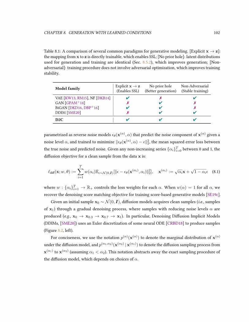
CHAPTER 8. GENERATION WITH LEARNED CONDITIONS 102
Table 8.1: A comparison of several common paradigms for generative modeling. [Explicit x→ z]:the mapping from x to z is directly trainable, which enables SSL; [No prior hole]: latent distributionsused for generation and training are identical (Sec. 8.5.2), which improves generation; [Non-adversarial]: training procedure does not involve adversarial optimization, which improves trainingstability.
Model family Explicit x→ z No prior hole Non-Adversarial(Enables SSL) (Better generation) (Stable training)
VAE [KW13, RM15], NF [DKB14] 4 7 4GAN [GPAM+14] 7 4 7BiGAN [DKD16, DBP+16] 4 4 7DDIM [SME20] 7 4 4
D2C 4 4 4
parametrized as reverse noise models εθ(x(α), α) that predict the noise component of x(α) given anoise level α, and trained to minimize ‖εθ(x(α), α) − ε‖22, the mean squared error loss betweenthe true noise and predicted noise. Given any non-increasing series αiTi=0 between 0 and 1, thediusion objective for a clean sample from the data x is:
`di(x;w, θ) :=
T∑i=1
w(αi)Eε∼N (0,I)[‖ε− εθ(x(αi), αi)‖22], x(αi) :=√αix +
√1− αiε (8.1)
where w : αiTi=1 → R+ controls the loss weights for each α. When w(α) = 1 for all α, werecover the denoising score matching objective for training score-based generative models [SE19c].
Given an initial sample x0 ∼ N (0, I), diusion models acquires clean samples (i.e., samplesof x1) through a gradual denoising process, where samples with reducing noise levels α areproduced (e.g., x0 → x0.3 → x0.7 → x1). In particular, Denoising Diusion Implicit Models(DDIMs, [SME20]) uses an Euler discretization of some neural ODE [CRBD18] to produce samples(Figure 8.2, left).
For conciseness, we use the notation p(α)(x(α)) to denote the marginal distribution of x(α)
under the diusion model, and p(α1,α2)(x(α2) | x(α1)) to denote the diusion sampling process fromx(α1) to x(α2) (assuming α1 < α2). This notation abstracts away the exact sampling procedure ofthe diusion model, which depends on choices of α.

CHAPTER 8. GENERATION WITH LEARNED CONDITIONS 103
8.4.1 Training diusion models
We use the notations in [SME20] to denote the α values and consider the forward diusion modelin [HJA20]; a non-Markovian version that motivates other sampling procedures can be found in[SME20], but the training procedure is largely identical. We refer to the reader to these two papersfor more details.
First, we dene the following diusion forward process for a series αtTt=0:
q(x(α1:T )|x(α0)) :=T∏t=1
q(x(αt)|x(αt−1)), (8.2)
q(x(αt)|x(αt−1)) := N(√
αtαt−1
x(αt−1),
(1− αt
αt−1
)I
), (8.3)
and from standard derivations for Gaussian we have that:
q(x(αt−1)|x(αt),x(α0)) = N( √
αt−1 − αt1− αt
x(α0) +αt(1− αt−1)
αt−1(1− αt)x(αt)︸ ︷︷ ︸
µ(x(αt),x(α0);αt,αt−1)
,1− αt−1
1− αt
(1− αt
αt−1
)I
).
(8.4)
As a variational approximation to the above, [HJA20] considered a specic type of pθ(x(αt−1)|x(αt)):
pθ(x(αt−1)|x(αt)) = N
(µθ(x
(αt);αt, αt−1), (σ(αt))2I), (8.5)
where µθ and σ(αt) are parameters, and we remove the superscript of pθ to indicate that there areno additional discretization steps in between (the sampling process is explicitly dened). Then, wehave the standard variational objective as follows:
L := Eq
[log q(x(αT )|x(α0)) +
T∑t=2
log q(x(αt−1)|x(αt),x(α0))−T∑t=1
log p(αt,αt−1)θ (x(αt−1)|x(αt))
]
≡ Eq
T∑t=2
DKL(q(x(αt−1)|x(αt),x(α0)))‖pθ(x(αt−1)|x(αt)))︸ ︷︷ ︸Lt−1
− log pθ(x(α0)|x(α1))
,where≡ denotes “equal up to a constant that does not depend on θ” and eachLt−1 is a KL divergencebetween two Gaussian distributions. Let us assume that the standard deviation of pθ(x(αt−1)|x(αt))

CHAPTER 8. GENERATION WITH LEARNED CONDITIONS 104
is equal to that of q(x(αt−1)|x(αt),x(α0))), which we denote as σ(αt). And thus:
Lt−1 = Eq[
1
2(σ(αt))2‖µθ(x(αt);αt, αt−1)− µ(x(αt),x(α0);αt, αt−1)‖22
]. (8.6)
With a particular reparametrization from µθ to εθ (which tries to model the noise vector at αt):
µθ(x(αt);αt, αt−1) =
√αt−1
αt
(x(αt) −
√αt−1 − αt√(1− αt)αt
· εθ(x(αt);αt)
), (8.7)
the objective function can be simplied to:
Lt−1 = Ex0,ε
[(αt−1 − αt)
2(σ(αt))2(1− αt)αt‖ε− εθ(x(αt);αt, αt−1)‖22
](8.8)
where x(αt) =√αtx0 +
√1− αtε. Intuitively, this is a weighted sum of mean-square errors
between the noise model εθ and the actual noise ε. Other weights can also be derived with dierentforward processes that are non-Markovian [SME20], and in practice, setting the weights to 1 isobserved to achieve decent performance for image generation.
8.4.2 DDIM sampling procedure
In this section, we discuss the detailed sampling procedure from x(0) ∼ N (0, I) (which is thedistribution with “all noise”2) to x(1) (which is the model distribution with “no noise”). Morespecically, we discuss a deterministic sampling procedure, which casts the generation procedureas an implicit model [SME20]. Compared to other procedures (such as the one in DDPM [HJA20]),this has the advantage of better sample quality when few steps are allowed to produce eachsample, as well as a near-invertible mapping between x(0) and x(1). We describe this procedure inAlgorithm 2, where we can choose dierent series of α to control how many steps (and throughwhich steps) we wish to draw a sample. The DDIM sampling procedure corresponds to a particulardiscretization to an ODE, we note that it is straightforward to also dene the sampling procedurebetween any two α values. Similarly, given an observation x(1) we can obtain the correspondinglatent code x(0) by sampling running Algorithm 2 with the sequence of α reversed.
2Technically, the maximum noise level αT should have αT → 0 but not equal to 0, but we can approximate thedistribution of x(αT ) with that of x(0) arbitrarily well in practice.
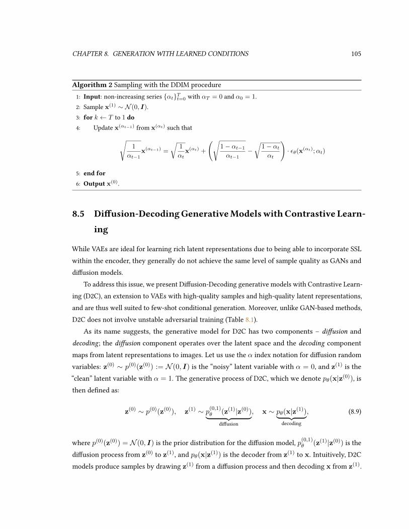
CHAPTER 8. GENERATION WITH LEARNED CONDITIONS 105
Algorithm 2 Sampling with the DDIM procedure1: Input: non-increasing series αtTt=0 with αT = 0 and α0 = 1.2: Sample x(1) ∼ N (0, I).3: for k ← T to 1 do4: Update x(αt−1) from x(αt) such that√
1
αt−1x(αt−1) =
√1
αtx(αt) +
(√1− αt−1
αt−1−√
1− αtαt
)· εθ(x(αt);αt)
5: end for6: Output x(0).
8.5 Diusion-DecodingGenerativeModelswithContrastive Learn-
ing
While VAEs are ideal for learning rich latent representations due to being able to incorporate SSLwithin the encoder, they generally do not achieve the same level of sample quality as GANs anddiusion models.
To address this issue, we present Diusion-Decoding generative models with Contrastive Learn-ing (D2C), an extension to VAEs with high-quality samples and high-quality latent representations,and are thus well suited to few-shot conditional generation. Moreover, unlike GAN-based methods,D2C does not involve unstable adversarial training (Table 8.1).
As its name suggests, the generative model for D2C has two components – diusion anddecoding; the diusion component operates over the latent space and the decoding componentmaps from latent representations to images. Let us use the α index notation for diusion randomvariables: z(0) ∼ p(0)(z(0)) := N (0, I) is the “noisy” latent variable with α = 0, and z(1) is the“clean” latent variable with α = 1. The generative process of D2C, which we denote pθ(x|z(0)), isthen dened as:
z(0) ∼ p(0)(z(0)), z(1) ∼ p(0,1)θ (z(1)|z(0))︸ ︷︷ ︸
diusion
, x ∼ pθ(x|z(1))︸ ︷︷ ︸decoding
, (8.9)
where p(0)(z(0)) = N (0, I) is the prior distribution for the diusion model, p(0,1)θ (z(1)|z(0)) is the
diusion process from z(0) to z(1), and pθ(x|z(1)) is the decoder from z(1) to x. Intuitively, D2Cmodels produce samples by drawing z(1) from a diusion process and then decoding x from z(1).

CHAPTER 8. GENERATION WITH LEARNED CONDITIONS 106
Decoding
Encoding
Diffusion
Figure 8.2: Illustration of components of a D2 model. On top of the encoding and decodingbetween x and z(1), we use a diusion model to generate z(1) from a Gaussian z(0). The red linesdescribe several smooth ODE trajectories from α = 0 to α = 1 corresponding to DDIM.
In order to train a D2C model, we use an inference model qφ(z(1)|x) that predicts properz(1) latent variables from x; this can directly incorporate SSL methods [XLZ+21], leading to thefollowing objective:
LD2C(θ, φ;w) := LD2(θ, φ;w) + λLC(qφ), (8.10)
LD2(θ, φ;w) := Ex∼pdata,z(1)∼qφ(z(1)|x)[− log p(x|z(1)) + `di(z(1);w, θ)], (8.11)
where `di is dened as in equation 8.1, LC(qφ) denotes any contrastive predictive coding ob-jective [vdOLV18] with rich data augmentations [HFW+19, CFGH20, CXH21, CKNH20, SE20b](details in Appendix B.6.1) and λ > 0 is a weight hyperparameter. The rst two terms, which wecall LD2, contains a “reconstruction loss” (− log p(x|z(1))) and a “diusion loss” over samples ofz(1) ∼ qφ(z(1)|x). We illustrate the D2C generative and inference models in Figure 8.2, and itstraining procedure in Appendix B.6.1.
8.5.1 Relationship to maximum likelihood
The D2 objective (LD2) appears similar to the original VAE objective (LVAE). Here, we make aninformal statement that the D2 objective function is deeply connected to the variational lowerbound of log-likelihood; we present the full statement and proof in Appendix A.6.1.
Theorem 12. (informal) For any valid αiTi=0, there exists some weights w : αiTi=1 → R+ for
the diusion objective such that −LD2 is a variational lower bound to the log-likelihood, i.e.,
−LD2(θ, φ; w) ≤ Epdata [log pθ(x)], (8.12)

CHAPTER 8. GENERATION WITH LEARNED CONDITIONS 107
where pθ(x) := Ex0∼p(0)(z(0))[pθ(x|z(0))] is the marginal probability of x under the D2C model.
Proof. (sketch) The diusion term `diff upper bounds the KL divergence between qφ(z1|x) andp
(1)θ (z(1)) for suitable weights [HJA20, SME20], which recovers a VAE objective.
8.5.2 D2C models address latent posterior mismatch in VAEs
While D2C is a special case of VAE, we argue that D2C is non-trivial in the sense that it ad-dresses a long-standing problem in VAE methods [TW17, TIY+19], namely the mismatch be-tween the prior distribution pθ(z) and the aggregate (approximate) posterior distribution qφ(z) :=
Epdata(x)[qφ(z|x)]. A mismatch could create “holes” [RLM18, HJ16, ASKV20] in the prior that theaggregate posterior fails to cover during training, resulting in worse sample quality, as many latentvariables used during generation are likely to never have been trained on. We formalize this notionin the following denition.
Denition 1 (Prior hole). Let p(z), q(z) be two distributions with supp(q) ⊆ supp(p). We say that
q has an (ε, δ)-prior hole with respect to (the prior) p for ε, δ ∈ (0, 1), δ > ε, if there exists a set
S ∈ supp(P ), such that∫S p(z) dz ≥ δ and
∫S q(z) dz ≤ ε.
Intuitively, if qφ(z) has a prior hole with large δ and small ε (e.g., inversely proportional to thenumber of training samples), then it is very likely that latent variables within the hole are neverseen during training (small ε), yet frequently used to produce samples (large δ). Most existingmethods address this problem by optimizing certain statistical divergences between qφ(z) andpθ(z), such as the KL divergence or Wasserstein distance [TBGS17]. However, we argue in thefollowing statement that prior holes might not be eliminated even if we optimize certain divergencevalues to be reasonably low, especially when qφ(z) is very exible. We present the formal statementand proof in Appendix A.6.2.
Theorem 13. (informal) Let pθ(z) = N (0, 1). For any ε > 0, there exists a distribution qφ(z) with
an (ε, 0.49)-prior hole, such that DKL(qφ‖pθ) ≤ log 23andW2(qφ, pθ) < γ for any γ > 0, where
W2 is the 2-Wasserstein distance.
Proof. (sketch) We construct a qφ that satises these properties (see gure). First, we truncate theGaussian and divide them into regions with same probability mass; then we support qφ over half ofthese regions (so δ > 0.49); nally, we show that the divergences are small enough.
3This is reasonably low for realistic VAE models (NVAE [VK20] reports a KL divergence of around 2810 nats).

CHAPTER 8. GENERATION WITH LEARNED CONDITIONS 108
p(z)q(z)
In contrast to addressing prior holes by optimization, diusion models eliminate prior holes byconstruction, since the diusion process from z(1) to z(0) is constructed such that the distributionof z(α) always converges to a standard Gaussian as α→ 0. As a result, the distribution of latentvariables used during training is arbitrarily close to that used in generation4, which is also the casein GANs. Therefore, our argument provides an explanation as to why we observe better samplequality results from GANs and diusion models than VAEs and NFs.
8.6 Few-shot Conditional Generation with D2C
In this section, we discuss how D2C can be used to learn to perform conditional generation from few-shot supervision. We note that D2C is only trained on images and not with any other data modalities(e.g., image-text pairs [RPG+21]) or supervision techniques (e.g., meta-learning [CD19, BV18]).
Algorithm 3 Conditional generation with D2C1: Input n examples (xi, ci)ni=1, property c.2: Acquire latents z(1)i ∼ qφ(z(1)|xi) for i ∈ [n];3: Train model rψ(c|z(1)) over (z(1)i , ci)ni=1
4: Sample latents with z(1) ∼ rψ(c|z(1)) · p(1)θ (z(1))
(unnormalized);5: Decode x ∼ pθ(x|z(1)).6: Output x.
Algorithm We describe the general algo-rithm for conditional generation from a fewimages in Algorithm 3. With a model overthe latent space (denoted as rψ(c|z(1))), wedraw conditional latents from an unnormal-ized distribution with the diusion prior (line4). This can be implemented in many wayssuch as rejection sampling or Langevin dynam-ics [NCB+17, SSDK+20, DN21].
Conditions from labeled examples Given a few labeled examples, we wish to produce diversesamples with a certain label. For labeled examples we can directly train a classier over thelatent space, which we denote as rψ(c|z(1)) with c being the class label and z(1) being the latent
4We expand this argument in Appendix A.6.2.

CHAPTER 8. GENERATION WITH LEARNED CONDITIONS 109
representation of x from qφ(z(1)|x). If these examples do not have labels (i.e., we merely want togenerate new samples similar to given ones), we can train a positive-unlabeled (PU) classier [EN08]where we assign “positive” to the new examples and “unlabeled” to training data. Then we usethe classier with the diusion model pθ(z(1)|z(0)) to produce suitable values of z(1), such as byrejecting samples from the diusion model that has a small rψ(c|z(1)).
Conditions from manipulation constraints Given a few labeled examples, here we wish tolearn how to manipulate images. Specically, we condition over the event that “x has label c but issimilar to image x”. Here rψ(c|z(1)) is the unnormalized product between the classier conditionalprobability and closeness to the latent z(1) of x (e.g., measured with RBF kernel). We implementline 4 of Alg. 3 with a Lanvegin-like procedure where we take a gradient step with respect to theclassier probability and then correct this gradient step with the diusion model. Unlike manyGAN-based methods [CK17, PHS+18, WLZ+18, IZZE17, XYXW21], D2C does not need to optimizean inversion procedure at evaluation time, and thus the latent value is much faster to compute;D2C is also better at retaining ne-grained features of the original image due to the reconstructionloss.
Detailed Algorithms In order to perform few-shot conditional generation, we need to imple-ment line 4 in Algorithm 3, where an unnormalized (energy-based) model is dened over therepresentations. After we have dened the energy-based model, we implement a procedure todraw samples from this unnormalized model. We note that our approach (marked in teal boxes) isonly one way of drawing valid samples, and not necessarily the optimal one. Furthermore, theseimplementations can also be done over the image space (which is the case for DDIM-I), which maycosts more to compute than over the latent space since more layers are needed in a neural networkto process it.
For generation from labels, we would dene the energy-based model over latents as the productof two components: the rst is the “prior” over z(1) as dened by the diusion model and thesecond is the “likliehood” of the label c being true given the latent variable z(1). This places highenergy values to the latent variables that are likely to occur under the diusion prior (so generatedimages are likely to have high quality) as well as latent variables that have the label c. To samplefrom this energy-based model, we perform a rejection sampling procedure, where we reject latentsamples from the diusion model that have low discrminator values. This procedure is describe inAlgorithm 4.
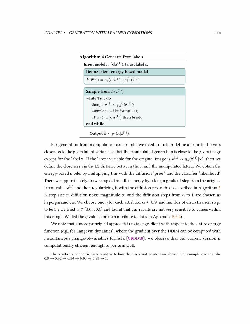
CHAPTER 8. GENERATION WITH LEARNED CONDITIONS 110
Algorithm 4 Generate from labelsInput model rψ(c|z(1)), target label c.
Dene latent energy-based model
E(z(1)) = rψ(c|z(1)) · p(1)θ (z(1))
Sample from E(z(1))
while True doSample z(1) ∼ p(1)θ (z(1));Sample u ∼ Uniform(0, 1);If u < rψ(c|z(1)) then break.
end while
Output x ∼ pθ(x|z(1)).
For generation from manipulation constraints, we need to further dene a prior that favorscloseness to the given latent variable so that the manipulated generation is close to the given imageexcept for the label z. If the latent variable for the original image is z(1) ∼ qφ(z(1)|x), then wedene the closeness via the L2 distance between the it and the manipulated latent. We obtain theenergy-based model by multiplying this with the diusion “prior” and the classier “likelihood”.Then, we approximately draw samples from this energy by taking a gradient step from the originallatent value z(1) and then regularizing it with the diusion prior; this is described in Algorithm 5.A step size η, diusion noise magnitude α, and the diusion steps from α to 1 are chosen ashyperparameters. We choose one η for each attribute, α ≈ 0.9, and number of discretization stepsto be 55; we tried α ∈ [0.65, 0.9] and found that our results are not very sensitive to values withinthis range. We list the η values for each attribute (details in Appendix B.6.2).
We note that a more principled approach is to take gradient with respect to the entire energyfunction (e.g., for Langevin dynamics), where the gradient over the DDIM can be computed withinstantaneous change-of-variables formula [CRBD18]; we observe that our current version iscomputationally ecient enough to perform well.
5The results are not particularly sensitive to how the discretization steps are chosen. For example, one can take0.9 → 0.92 → 0.96 → 0.98 → 0.99 → 1.
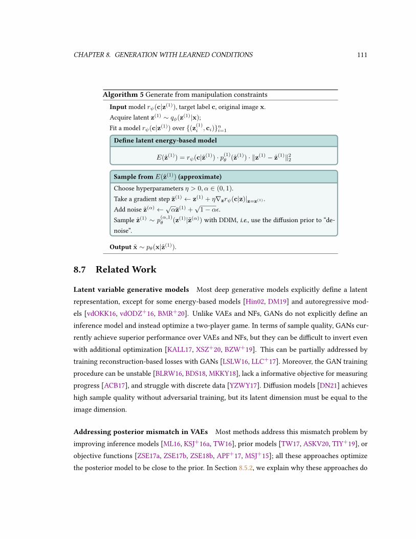
CHAPTER 8. GENERATION WITH LEARNED CONDITIONS 111
Algorithm 5 Generate from manipulation constraintsInput model rψ(c|z(1)), target label c, original image x.Acquire latent z(1) ∼ qφ(z(1)|x);Fit a model rψ(c|z(1)) over (z(1)i , ci)ni=1
Dene latent energy-based model
E(z(1)) = rψ(c|z(1)) · p(1)θ (z(1)) · ‖z(1) − z(1)‖22
Sample from E(z(1)) (approximate)
Choose hyperparameters η > 0, α ∈ (0, 1).Take a gradient step z(1) ← z(1) + η∇zrψ(c|z)|z=z(1) .Add noise z(α) ← √αz(1) +
√1− αε.
Sample z(1) ∼ p(α,1)θ (z(1)|z(α)) with DDIM, i.e., use the diusion prior to “de-
noise”.
Output x ∼ pθ(x|z(1)).
8.7 Related Work
Latent variable generative models Most deep generative models explicitly dene a latentrepresentation, except for some energy-based models [Hin02, DM19] and autoregressive mod-els [vdOKK16, vdODZ+16, BMR+20]. Unlike VAEs and NFs, GANs do not explicitly dene aninference model and instead optimize a two-player game. In terms of sample quality, GANs cur-rently achieve superior performance over VAEs and NFs, but they can be dicult to invert evenwith additional optimization [KALL17, XSZ+20, BZW+19]. This can be partially addressed bytraining reconstruction-based losses with GANs [LSLW16, LLC+17]. Moreover, the GAN trainingprocedure can be unstable [BLRW16, BDS18, MKKY18], lack a informative objective for measuringprogress [ACB17], and struggle with discrete data [YZWY17]. Diusion models [DN21] achieveshigh sample quality without adversarial training, but its latent dimension must be equal to theimage dimension.
Addressing posterior mismatch in VAEs Most methods address this mismatch problem byimproving inference models [ML16, KSJ+16a, TW16], prior models [TW17, ASKV20, TIY+19], orobjective functions [ZSE17a, ZSE17b, ZSE18b, APF+17, MSJ+15]; all these approaches optimizethe posterior model to be close to the prior. In Section 8.5.2, we explain why these approaches do

CHAPTER 8. GENERATION WITH LEARNED CONDITIONS 112
not necessarily remove large “prior holes”, so their sample qualities remain relatively poor evenafter many layers [VK20, Chi20]. Other methods adopt a “two-stage” approach [DW19], which tsa generative model over the latent space of autoencoders [vdOVK17, ROV19, DJP+20, RPG+21].
Conditional generation with unconditional models To perform conditional generation overan unconditional LVGM, most methods assume access to a discriminative model (e.g., a classier);the latent space of the generator is then modied to change the outputs of the discriminative model.The disciminative model can operate on either the image space [NCB+17, PWS+21, DN21] or thelatent space [SGTZ20, XYXW21]. For image space discriminative models, plug-and-play generativenetworks [NCB+17] control the attributes of generated images via Langevin dynamics [RR98];these ideas are also explored in diusion models [SSDK+20]. Image manipulation methods arebased on GANs often operate with latent space discriminators [SGTZ20, XYXW21]. However, thesemethods have some trouble manipulating real images because of imperfect reconstruction [ZZZZ19,BZW+19]. This is not a problem in D2C since a reconstruction objective is optimized.
8.8 Experiments
We examine the conditional and unconditional generation qualities of D2C over CIFAR-10 [KSH12],CIFAR-100 [KSH12], fMoW [CFWM18], CelebA-64 [LLWT15], CelebA-HQ-256 [KALL17], andFFHQ-256 [KLA18]. Our D2C implementation is based on the state-of-the-art NVAE [VK20] autoen-coder structure, the U-Net diusion model [HJA20], and the MoCo-v2 contrastive representationlearning method [CFGH20]. We keep the diusion series hyperparameter αiTi=1 identical toensure a fair comparison with dierent diusion models. For the contrastive weight hyperparameterλ in Equation 8.10, we consider the value of λ = 10−4 based on the relative scale between theLC and LD2; we nd that the results are relatively insensitive to λ. We use 100 diusion steps forDDIM and D2C unless mentioned otherwise, as running with longer steps is not computationallyeconomical despite tiny gains in FID [SME20]. We include additional training details, such asarchitectures, optimizers and learning rates in Appendix B.6.2.
8.8.1 Unconditional generation
For unconditional generation, we measure the sample quality of images using the Frechet InceptionDistance (FID, [HRU+17]) with 50,000 images. In particular, we extensively evaluate NVAE [VK20]and DDIM [SME20], a competitive VAE model and a competitive diusion model as baselines

CHAPTER 8. GENERATION WITH LEARNED CONDITIONS 113
Table 8.2: Quality of representations and generations with LVGMs.
Model CIFAR-10 CIFAR-100 fMoWFID ↓ MSE ↓ Acc ↑ FID ↓ MSE ↓ Acc ↑ FID ↓ MSE ↓ Acc ↑
NVAE [VK20] 36.4 0.25 18.8 42.5 0.53 4.1 82.25 0.30 27.7DDIM [SME20] 4.16 2.5 22.5 10.16 3.2 2.2 37.74 3.0 23.5
D2C (Ours) 10.15 0.76 76.02 14.62 0.44 42.75 44.7 2.33 66.9
Figure 8.3: Generated samples on CIFAR-10, fMoW, and FFHQ.
because we can directly obtain features from them without additional optimization steps6. Forthem, we report mean-squared reconstruction error (MSE, summed over all pixels, pixels normalizedto [0, 1]) and linear classication accuracy (Acc., measured in percentage) over z1 features for thetest set.
We report sample quality results7 in Tables 8.2, and 8.3. For FID, we outperform NVAE in alldatasets and outperform DDIM on CelebA-64 and CelebA-HQ-256, which suggests our results arecompetitive with state-of-the-art non-adversarial generative models. In Table 8.2, we additionallycompare NVAE, DDIM and D2C in terms of reconstruction and linear classication accuracy.As all three methods contain reconstruction losses, the MSE values are low and comparable.However, D2C enjoys much better linear classication accuracy than the other two thanks tothe contrastive SSL component. We further note that training the same contrastive SSL methodwithout LD2 achieves slightly higher 78.3% accuracy on CIFAR-10. We tried improving this viaResNet [HZRS15] encoders, but this signicantly increased reconstruction error, possibly due toloss of information in average pooling layers.
6For DDIM, the latent representations x(0) are obtained by reversing the neural ODE process.7Due to space limits, we place additional CIFAR-10 results in Appendix B.6.3.

CHAPTER 8. GENERATION WITH LEARNED CONDITIONS 114
Table 8.3: FID scores over dierent faces dataset with LVGMs.
Model CelebA-64 CelebA-HQ-256 FFHQ-256
NVAE [VK20] 13.48 40.26 26.02DDIM [SME20] 6.53 25.6 -
D2C (Ours) 5.7 18.74 13.04
Table 8.4: Sample quality as a function of diusion steps.
CIFAR-10 CIFAR-100 CelebA-64Steps 10 50 100 10 50 100 10 50 100
DDPM [HJA20] 41.07 8.01 5.78 50.27 21.37 16.72 33.12 18.48 13.93DDIM [SME20] 13.36 4.67 4.16 23.34 11.69 10.16 17.33 9.17 6.53D2C (Ours) 17.71 10.11 10.15 23.16 14.62 14.46 17.32 6.8 5.7
8.8.2 Few-shot conditional generation from examples
We demonstrate the advantage of D2C representations by performing few-shot conditional genera-tion over labels. We consider two types of labeled examples: one has binary labels for which wetrain a binary classier; the other is positive-only labeled (e.g., images of female class) for which wetrain a PU classier. Our goal here is to generate a diverse group of images with a certain label. Weevaluate and compare three models: D2C, NVAE and DDIM. We train a classier rψ(c|z) over thelatent space of these models; we also train a image space classier and use it with DDIM (denoted asDDIM-I). We run Algorithm 3 for these models, where line 4 is implemented via rejection sampling.As our goal is to compare dierent models, we leave more sophisticated methods [DN21] as futurework.
We consider performing 8 conditional generation tasks over CelebA-64 with 2 binary classiers(trained over 100 samples, 50 for each class) and 4 PU classiers (trained over 100 positively labeledand 10k unlabeled samples). We also report a “naive” approach where we use all the training images(regardless of labels) and compute its FID with the corresponding subset of images (e.g., all imagesversus blond images). In Table 8.5, we report the FID score between generated images (5k samples)and real images of the corresponding label. These results suggest that D2C outperforms the otherapproaches, and is the only one that performs better than the “naive” approach in most cases,illustrating the advantage of contrastive representations for few-shot conditional generation.

CHAPTER 8. GENERATION WITH LEARNED CONDITIONS 115
Table 8.5: FID scores for few-shot conditional generation with various types of labeled examples.Naive performs very well for non-blond due to class percentages.
Method Classes (% in train set) D2C DDIM NVAE DDIM-I Naive
Binary
Male (42%) 13.44 38.38 41.07 29.03 26.34Female (58%) 9.51 19.25 16.57 15.17 18.72Blond (15%) 17.61 31.39 31.24 29.09 27.51Non-Blond (85%) 8.94 9.67 16.73 19.76 3.77
PU
Male (42%) 16.39 37.03 42.78 19.60 26.34Female (58%) 12.21 15.42 18.36 14.96 18.72Blond (15%) 10.09 30.20 31.06 76.52 27.51Non-Blond (85%) 9.09 9.70 17.98 9.90 3.77
8.8.3 Few-shot conditional generation from manipulation constraints
Finally, we consider image manipulation where we use binary classiers that are learned over50 labeled instances for each class. We perform Amazon Mechanical Turk (AMT) evaluationsover two attributes in the CelebA-256 dataset, blond and red lipstick, over D2C, DDIM, NVAEand StyleGAN2 [KLA+20] (see Figure 8.4). The evaluation is double-blinded: neither we nor theevaluators know the correspondence between generated image and underlying model during thestudy. We include more details (algorithm, setup and human evaluation) in Appendix B.6.2 andadditional qualitative results (such as beard and gender attributes) in Appendix B.6.3.
In Figure 8.5, we show the percentage of manipulations preferred by AMT evaluators for eachmodel; D2C slightly outperforms StyleGAN2 for blond and signicantly outperforms StyleGAN2for red lipstick. When we compare D2C with only StyleGAN2, D2C is preferred over 51.5% forblond and 60.8% for red lipstick. An additional advantage of D2C is that the manipulation is muchfaster than StyleGAN2, since the latter requires additional optimization over the latent space toimprove reconstruction [ZSZZ20]. On the same Nvidia 1080Ti GPU, it takes 0.013 seconds to obtainthe latent code in D2C, while the same takes 8 seconds [ZSZZ20] for StyleGAN2 (615× slower). Asdecoding is very fast for both models, D2C generations are around two orders of magnitude fasterto produce.
8.9 Discussions
We introduced D2C, a VAE-based generative model with a latent space suitable for few-shotconditional generation. To our best knowledge, our model is the rst unconditional VAE to

CHAPTER 8. GENERATION WITH LEARNED CONDITIONS 116
Original D2C StyleGAN2 NVAE DDIM
Figure 8.4: Image manipulation results for blond (top) and red lipstick (bottom). D2C is better thanStyleGAN2 at preserving details of the original image, such as eyes, earrings, and background.
0.0 0.1 0.2 0.3 0.4 0.5
D2C
StyleGAN2
NVAE
DDIM
Red lipstick
0.0 0.1 0.2 0.3
D2C
StyleGAN2
NVAE
DDIM
Blond
Figure 8.5: AMT evaluation over image manipulations. x-axis shows the percentage that theevaluator selects the image generated from the corresponding model out of 4 images from eachmodel.

CHAPTER 8. GENERATION WITH LEARNED CONDITIONS 117
demonstrate superior image manipulation performance than StyleGAN2, which is surprising givenour use of a regular NVAE architecture. We believe that with better architectures, such as designsfrom StyleGAN2 or Transformers [HZ21], D2C can achieve even better performance. It is alsointeresting to formally investigate the integration between D2C and other types of conditions onthe latent space, as well as training D2C in conjunction with other domains and data modalities,such as text [RPG+21], in a fashion that is similar to semi-supervised learning. Nevertheless, wenote that our model have to be used properly in order to mitigate potential negative societal impacts,such as deep fakes.
Part III
Inference via Supervised Learning
118
Chapter 9
Learning Kernels for Markov ChainMonte Carlo
In the previous part, we discussed how supervised learning methods can be integrated into uncon-ditional and conditional generative models, such as generative adversarial networks and variationalautoencoders. In this part, we discuss how supervised learning can be used to improve inferencemethods, starting with Bayesian inference.
Markov Chain Monte Carlo (MCMC) methods are regarded as the “golden standard” of Bayesianinference, but existing MCMC methods are either based on general-purpose and domain-agnosticschemes that can lead to slow convergence, or based on problem-specic proposals hand-crafted byan expert. As a result, MCMC methods are falling out of favor compared to approximate inferencemethods (such as variational inference) despite being asymptotically exact.
In this chapter, we propose A-NICE-MC, a novel method that uses supervised learning toautomatically design ecient Markov chain kernels tailored for a specic domain. First, we proposean ecient likelihood-free supervised learning (adversarial training) method to train a Markovchain and mimic a given data distribution. Then, we leverage exible volume preserving ows toobtain parametric kernels for MCMC. Using a bootstrap approach, we show how to train ecientMarkov chains to sample from a prescribed posterior distribution by iteratively improving thequality of both the model and the samples. Empirical results demonstrate that A-NICE-MC combinesthe strong guarantees of MCMC with the expressiveness of deep neural networks, and is able tosignicantly outperform competing methods such as Hamiltonian Monte Carlo.
This chapter is previously published in [SZE17]. Shengjia Zhao and Daniel Levy contributedto the contents of this chapter. My contributions include conceiving the idea, implementing the
119

CHAPTER 9. LEARNING KERNELS FOR MARKOV CHAIN MONTE CARLO 120
algorithms and executing the experiments.
9.1 Introduction
Variational inference (VI) and Monte Carlo (MC) methods are two key approaches to deal withcomplex probability distributions in machine learning. The former approximates an intractabledistribution by solving a variational optimization problem to minimize a divergence measure withrespect to some tractable family. The latter approximates a complex distribution using a smallnumber of typical states, obtained by sampling ancestrally from a proposal distribution or iterativelyusing a suitable Markov chain (Markov Chain Monte Carlo, or MCMC).
Recent progress in deep learning has vastly advanced the eld of variational inference. Notableexamples include black-box variational inference and variational autoencoders [RGB14, KW13,RMW14], which enabled variational methods to benet from the expressive power of deep neuralnetworks, and adversarial training [GPAM+14, ML16], which allowed the training of new familiesof implicit generative models with ecient ancestral sampling.
MCMC methods, on the other hand, have not beneted as much from these recent advancements.Unlike variational approaches, MCMC methods are iterative in nature and do not naturally lendthemselves to the use of expressive function approximators [SKW15, DFHSJR01]. Even evaluatingan existing MCMC technique is often challenging, and natural performance metrics are intractableto compute [GM15, GDVM16, GM17, EGSS14]. Dening an objective to improve the performanceof MCMC that can be easily optimized in practice over a large parameter space is itself a dicultproblem [MWHDF12, BDX04].
To address these limitations, we introduce A-NICE-MC, a new method for training exibleMCMC kernels, e.g., parameterized using (deep) neural networks. Given a kernel, we view theresulting Markov Chain as an implicit generative model, i.e., one where sampling is ecient butevaluating the (marginal) likelihood is intractable. We then propose supervised training as aneective, likelihood-free method for training a Markov chain to match a target distribution.
First, we show it can be used in a learning setting to directly approximate an (empirical) datadistribution. We then use the approach to train a Markov Chain to sample eciently from amodel prescribed by an analytic expression (e.g., a Bayesian posterior distribution), the classic usecase for MCMC techniques. We leverage exible volume preserving ow models [DKB14] and a“bootstrap” technique to automatically design powerful domain-specic proposals that combine theguarantees of MCMC and the expressiveness of neural networks. Finally, we propose a method that

CHAPTER 9. LEARNING KERNELS FOR MARKOV CHAIN MONTE CARLO 121
decreases autocorrelation and increases the eective sample size of the chain as training proceeds.We demonstrate that these trained operators are able to signicantly outperform traditional ones,such as Hamiltonian Monte Carlo, in various domains.
9.2 Notations and Problem Setup
A sequence of continuous random variables xt∞t=0, xt ∈ Rn, is drawn through the followingMarkov chain:
x0 ∼ π0 xt+1 ∼ Tθ(xt+1|xt)
where Tθ(·|x) is a time-homogeneous stochastic transition kernel parametrized by θ ∈ Θ andπ0 is some initial distribution for x0. In particular, we assume that Tθ is dened through animplicit generative model fθ(·|x, v), where v ∼ p(v) is an auxiliary random variable, and fθ is adeterministic transformation (e.g., a neural network). Let πtθ denote the distribution for xt. If theMarkov chain is both irreducible and positive recurrent, then it has an unique stationary distributionπθ = lim
t→∞ πtθ . We assume that this is the case for all the parameters θ ∈ Θ.
Let pd(x) be a target distribution over x ∈ Rn, e.g, a data distribution or an (intractable)posterior distribution in a Bayesian inference setting. Our objective is to nd a Tθ such that itachieves:
1. Low bias: The stationary distribution is close to the target distribution (minimize |πθ − pd|).
2. Eciency: πtθ∞t=0 converges quickly (minimize t such that |πtθ − pd| < δ).
3. Low variance: Samples from one chain xt∞t=0 should be as uncorrelated as possible(minimize autocorrelation of xt∞t=0).
We think of πθ as a stochastic generative model, which can be used to eciently producesamples with certain characteristics (specied by pd), allowing for ecient Monte Carlo estimates.We consider two settings for specifying the target distribution. The rst is a learning setting wherewe do not have an analytic expression for pd(x), but we have access to typical samples simi=1 ∼ pd;in the second case we have an analytic expression for pd(x), possibly up to a normalization constant,but no access to samples. The two cases are discussed in Sections 9.3 and 9.4 respectively.

CHAPTER 9. LEARNING KERNELS FOR MARKOV CHAIN MONTE CARLO 122
9.3 Adversarial Training for Markov Chains
Consider the setting where we have direct access to samples from pd(x). Assume that the transitionkernel Tθ(xt+1|xt) is the following implicit generative model:
v ∼ p(v) xt+1 = fθ(xt, v) (9.1)
Assuming a stationary distribution πθ(x) exists, the value of πθ(x) is typically intractable tocompute. The marginal distribution πtθ(x) at time t is also intractable, since it involves integrationover all the possible paths (of length t) to x. However, we can directly obtain samples from πtθ,which will be close to πθ if t is large enough (assuming ergodicity). This aligns well with the ideaof generative adversarial networks (GANs), a likelihood free method which only requires samplesfrom the model.
Generative Adversarial Network (GAN) [GPAM+14] is a framework for training deep gen-erative models using a two player minimax game. A generator network G generates samplesby transforming a noise variable z ∼ p(z) into G(z). A discriminator network D(x) is trainedto distinguish between “fake” samples from the generator and “real” samples from a given datadistribution pd. Formally, this denes the following objective (Wasserstein GAN, from [ACB17])
minG
maxD
V (D,G) = minG
maxD
Ex∼pd [D(x)]− Ez∼p(z)[D(G(z))] (9.2)
In our setting, we could assume pd(x) is the empirical distribution from the samples, and choosez ∼ π0 and let Gθ(z) be the state of the Markov Chain after t steps, which is a good approximationof πθ if t is large enough. However, optimization is dicult because we do not know a reasonablet in advance, and the gradient updates are expensive due to backpropagation through the entirechain.
Therefore, we propose a more ecient approximation, called Markov GAN (MGAN):
minθ
maxD
Ex∼pd [D(x)]− λEx∼πbθ [D(x)]− (1− λ)Exd∼pd,x∼Tmθ (x|xd)[D(x)] (9.3)
where λ ∈ (0, 1), b ∈ N+,m ∈ N+ are hyperparameters, x denotes “fake” samples from thegenerator and Tmθ (x|xd) denotes the distribution of x when the transition kernel is applied mtimes, starting from some “real” sample xd.
We use two types of samples from the generator for training, optimizing θ such that the sampleswill fool the discriminator:

CHAPTER 9. LEARNING KERNELS FOR MARKOV CHAIN MONTE CARLO 123
Figure 9.1: Visualizing samples of π1 to π50 (each row) from a model trained on the MNIST dataset.Consecutive samples can be related in label (red box), inclination (green box) or width (blue box).
1. Samples obtained after b transitions x ∼ πbθ , starting from x0 ∼ π0.
2. Samples obtained after m transitions, starting from a data sample xd ∼ pd.
Intuitively, the rst condition encourages the Markov Chain to converge towards pd overrelatively short runs (of length b). The second condition enforces that pd is a xed point for thetransition operator.1 Instead of simulating the chain until convergence, which will be especiallytime-consuming if the initial Markov chain takes many steps to mix, the generator would runonly (b + m)/2 steps on average. Empirically, we observe better training times by uniformlysampling b from [1, B] and m from [1,M ] respectively in each iteration, so we use B and M as thehyperparameters for our experiments.
9.3.1 Example: Generative Model for Images
We experiment with a distribution pd over images, such as digits (MNIST) and faces (CelebA). In theexperiments, we parametrize fθ to have an autoencoding structure, where the auxiliary variablev ∼ N (0, I) is directly added to the latent code of the network serving as a source of randomness:
z = encoderθ(xt) z′ = ReLU(z + βv) xt+1 = decoderθ(z′) (9.4)
where β is a hyperparameter we set to 0.1. While sampling is inexpensive, evaluating probabilitiesaccording to Tθ(·|xt) is generally intractable as it would require integration over v. The startingdistribution π0 is a factored Gaussian distribution with mean and standard deviation being themean and standard deviation of the training set. We include all the details, which ares based on theDCGAN [RMC15] architecture, in Appendix B.7.4. All the models are trained with the gradientpenalty objective for Wasserstein GANs [GAA+17, ACB17], where λ = 1/3, B = 4 and M = 3.
We visualize the samples generated from our trained Markov chain in Figures 9.1 and 9.3, whereeach row shows consecutive samples from the same chain. From Figure 9.1, it is clear that xt+1 isrelated to xt in terms of high-level properties, such as digit identity (label). Our model learns to nd
1We provide a more rigorous justication in Appendix B.7.2.

CHAPTER 9. LEARNING KERNELS FOR MARKOV CHAIN MONTE CARLO 124
Figure 9.2: Tθ(yt+1|yt). Figure 9.3: Samples of π1 to π30 from models (top: without shortcut con-nections; bottom: with shortcut) trained on the CelebA dataset.
and move between the modes of the dataset, instead of generating a single sample ancestrally. Thisis drastically dierent from other iterative generative models trained with maximum likelihood,such as Generative Stochastic Networks (GSN, [BTLAY14]) and Infusion Training (IF, [BHV17]),because when we train Tθ(xt+1|xt) we are not specifying a particular target for xt+1. In fact, tomaximize the discriminator score the model (generator) may choose to generate some xt+1 near adierent mode.
To further investigate the frequency of various modes in the stationary distribution, we considerthe class-to-class transition probabilities for MNIST. We run one step of the transition operatorstarting from real samples where we have class labels y ∈ 0, . . . , 9, and classify the generatedsamples with a CNN. We are thus able to quantify the transition matrix for labels in Figure 9.2.Results show that class probabilities are fairly uniform and range between 0.09 and 0.11.
Although it seems that the MGAN objective encourages rapid transitions between dierentmodes, it is not always the case. In particular, as shown in Figure 9.3, adding residual connections[HZRS16] and highway connections [SGS15] to an existing model can signicantly increase thetime needed to transition between modes. This suggests that the time needed to transition betweenmodes can be aected by the architecture we choose for fθ(xt, v). If the architecture introduces aninformation bottleneck which forces the model to “forget” xt, then xt+1 will have higher chanceto occur in another mode; on the other hand, if the model has shortcut connections, it tends togenerate xt+1 that are close to xt. The increase in autocorrelation will hinder performance ifsamples are used for Monte Carlo estimates.

CHAPTER 9. LEARNING KERNELS FOR MARKOV CHAIN MONTE CARLO 125
9.4 Adversarial Training for Markov Chain Monte Carlo
We now consider the setting where the target distribution pd is specied by an analytic expression:
pd(x) ∝ exp(−U(x)) (9.5)
where U(x) is a known energy function and the normalization constant in Equation (9.5) might beintractable to compute. This form is very common in Bayesian statistics [Gre95], computationalphysics [JM12] and graphics [LB14]. Compared to the setting in Section 9.3, there are two additionalchallenges:
1. We want to train a Markov chain such that the stationary distribution πθ is exactly pd;
2. We do not have direct access to samples from pd during training.
9.4.1 Exact Sampling Through MCMC
We use ideas from the Markov Chain Monte Carlo (MCMC) literature to satisfy the rst condition andguarantee that πtθ∞t=0 will asymptotically converge to pd. Specically, we require the transitionoperator Tθ(·|x) to satisfy the detailed balance condition:
pd(x)Tθ(x′|x) = pd(x
′)Tθ(x|x′) (9.6)
for all x and x′. This condition can be satised using Metropolis-Hastings (MH), where a sample x′
is rst obtained from a proposal distribution gθ(x′|x) and accepted with the following probability:
Aθ(x′|x) = min
(1,pd(x
′)
pd(x)
gθ(x|x′)gθ(x′|x)
)= min
(1, exp(U(x)− U(x′))
gθ(x|x′)gθ(x′|x)
)(9.7)
Therefore, the resulting MH transition kernel can be expressed as Tθ(x′|x) = gθ(x′|x)Aθ(x
′|x) (ifx 6= x′), and it can be shown that pd is stationary for Tθ(·|x) [Has70].
The idea is then to optimize for a good proposal gθ(x′|x). We can set gθ directly as in Equation(9.1) (if fθ takes a form where the probability gθ can be computed eciently), and attempt to optimizethe MGAN objective in Eq. (9.3) (assuming we have access to samples from pd, a challenge we willaddress later). Unfortunately, Eq. (9.7) is not dierentiable - the setting is similar to policy gradientoptimization in reinforcement learning. In principle, score function gradient estimators (such asREINFORCE [Wil92]) could be used in this case; in our experiments, however, this approach leads

CHAPTER 9. LEARNING KERNELS FOR MARKOV CHAIN MONTE CARLO 126
to extremely low acceptance rates. This is because during initialization, the ratio gθ(x|x′)/gθ(x′|x)
can be extremely low, which leads to low acceptance rates and trajectories that are not informativefor training. While it might be possible to optimize directly using more sophisticated techniquesfrom the RL literature, we introduce an alternative approach based on volume preserving dynamics.
9.4.2 Hamiltonian Monte Carlo and Volume Preserving Flow
To gain some intuition to our method, we introduce Hamiltonian Monte Carlo (HMC) and volumepreserving ow models [N+11]. HMC is a widely applicable MCMC method that introduces anauxiliary “velocity” variable v to gθ(x′|x). The proposal rst draws v from p(v) (typically a factoredGaussian distribution) and then obtains (x′, v′) by simulating the dynamics (and inverting v at theend of the simulation) corresponding to the Hamiltonian
H(x, v) = v>v/2 + U(x) (9.8)
where x and v are iteratively updated using the leapfrog integrator (see [N+11]). The transitionfrom (x, v) to (x′, v′) is deterministic, invertible and volume preserving, which means that
gθ(x′, v′|x, v) = gθ(x, v|x′, v′) (9.9)
MH acceptance (9.7) is computed using the distribution p(x, v) = pd(x)p(v), where the acceptanceprobability is p(x′, v′)/p(x, v) since gθ(x′, v′|x, v)/gθ(x, v|x′, v′) = 1. We can safely discard v′
after the transition since x and v are independent.Let us return to the case where the proposal is parametrized by a neural network; if we could
satisfy Equation 9.9 then we could signicantly improve the acceptance rate compared to the“REINFORCE” setting. Fortunately, we can design such an proposal by using a volume preservingow model [DKB14].
A ow model [DKB14, RM15, KSJ+16b, GDE17] denes a generative model for x ∈ Rn througha bijection f : h→ x, where h ∈ Rn have the same number of dimensions as x with a xed priorpH(h) (typically a factored Gaussian). In this form, pX(x) is tractable because
pX(x) = pH(f−1(x))
∣∣∣∣det∂f−1(x)
∂x
∣∣∣∣−1
(9.10)
and can be optimized by maximum likelihood.In the case of a volume preserving ow model f , the determinant of the Jacobian ∂f(h)
∂h is one.
CHAPTER 9. LEARNING KERNELS FOR MARKOV CHAIN MONTE CARLO 127
Such models can be constructed using additive coupling layers, which rst partition the input intotwo parts, y and z, and then dene a mapping from (y, z) to (y′, z′) as:
y′ = y z′ = z +m(y) (9.11)
where m(·) can be an expressive function, such as a neural network. By stacking multiple couplinglayers the model becomes highly expressive. Moreover, once we have the forward transformation f ,the backward transformation f−1 can be easily derived. This family of models are called Non-linear
Independent Components Estimation (NICE) [DKB14].
9.4.3 A NICE Proposal
HMC has two crucial components. One is the introduction of the auxiliary variable v, whichprevents random walk behavior; the other is the symmetric proposal in Equation (9.9), which allowsthe MH step to only consider p(x, v). In particular, if we simulate the Hamiltonian dynamics (thedeterministic part of the proposal) twice starting from any (x, v) (without MH or resampling v),we will always return to (x, v).
Auxiliary variables can be easily integrated into neural network proposals. However, it is hardto obtain symmetric behavior. If our proposal is deterministic, then fθ(fθ(x, v)) = (x, v) shouldhold for all (x, v), a condition which is dicult to achieve2. Therefore, we introduce a proposalwhich satises Eq. (9.9) for any θ, while preventing random walk in practice by resampling v afterevery MH step.
Our proposal considers a NICE model fθ(x, v) with its inverse f−1θ , where v ∼ p(v) is the
auxiliary variable. We draw a sample x′ from the proposal gθ(x′, v′|x, v) using the followingprocedure:
1. Randomly sample v ∼ p(v) and u ∼ Uniform[0, 1];
2. If u > 0.5, then (x′, v′) = fθ(x, v);
3. If u ≤ 0.5, then (x′, v′) = f−1θ (x, v).
We call this proposal a NICE proposal and introduce the following theorem.
2The cycle consistency loss (as in CycleGAN [ZPIE17]) introduces a regularization term for this condition; we addedthis to the REINFORCE objective but were not able to achieve satisfactory results.
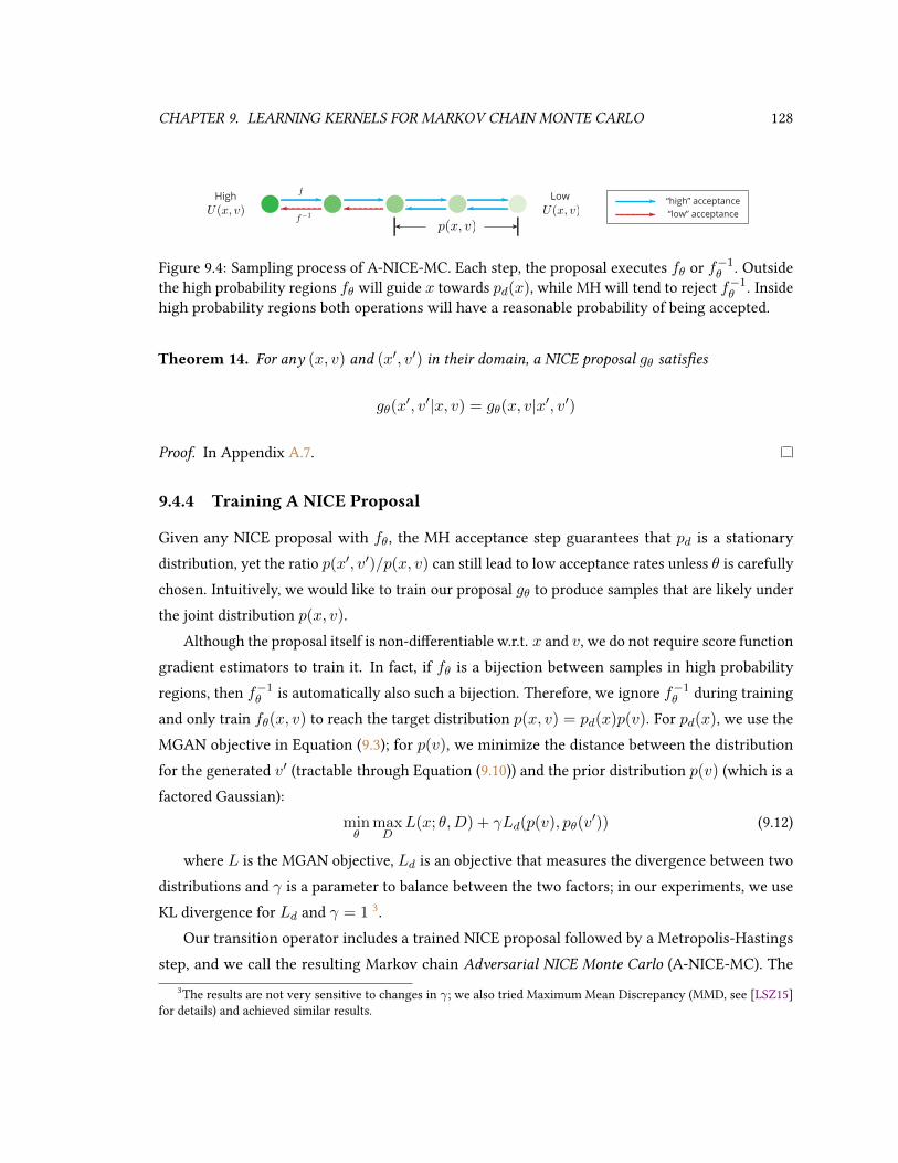
CHAPTER 9. LEARNING KERNELS FOR MARKOV CHAIN MONTE CARLO 128
f
f−1
High “high” acceptance“low” acceptanceU(x, v)
LowU(x, v)
p(x, v)
Figure 9.4: Sampling process of A-NICE-MC. Each step, the proposal executes fθ or f−1θ . Outside
the high probability regions fθ will guide x towards pd(x), while MH will tend to reject f−1θ . Inside
high probability regions both operations will have a reasonable probability of being accepted.
Theorem 14. For any (x, v) and (x′, v′) in their domain, a NICE proposal gθ satises
gθ(x′, v′|x, v) = gθ(x, v|x′, v′)
Proof. In Appendix A.7.
9.4.4 Training A NICE Proposal
Given any NICE proposal with fθ, the MH acceptance step guarantees that pd is a stationarydistribution, yet the ratio p(x′, v′)/p(x, v) can still lead to low acceptance rates unless θ is carefullychosen. Intuitively, we would like to train our proposal gθ to produce samples that are likely underthe joint distribution p(x, v).
Although the proposal itself is non-dierentiable w.r.t. x and v, we do not require score functiongradient estimators to train it. In fact, if fθ is a bijection between samples in high probabilityregions, then f−1
θ is automatically also such a bijection. Therefore, we ignore f−1θ during training
and only train fθ(x, v) to reach the target distribution p(x, v) = pd(x)p(v). For pd(x), we use theMGAN objective in Equation (9.3); for p(v), we minimize the distance between the distributionfor the generated v′ (tractable through Equation (9.10)) and the prior distribution p(v) (which is afactored Gaussian):
minθ
maxD
L(x; θ,D) + γLd(p(v), pθ(v′)) (9.12)
where L is the MGAN objective, Ld is an objective that measures the divergence between twodistributions and γ is a parameter to balance between the two factors; in our experiments, we useKL divergence for Ld and γ = 1 3.
Our transition operator includes a trained NICE proposal followed by a Metropolis-Hastingsstep, and we call the resulting Markov chain Adversarial NICE Monte Carlo (A-NICE-MC). The
3The results are not very sensitive to changes in γ; we also tried Maximum Mean Discrepancy (MMD, see [LSZ15]for details) and achieved similar results.

CHAPTER 9. LEARNING KERNELS FOR MARKOV CHAIN MONTE CARLO 129
Figure 9.5: Left: Samples from a model with shortcut connections trained with ordinary discrimina-tor. Right: Samples from the same model trained with a pairwise discriminator.
sampling process is illustrated in Figure 9.4. Intuitively, if (x, v) lies in a high probability region,then both fθ and f−1
θ should propose a state in another high probability region. If (x, v) is in alow-probability probability region, then fθ would move it closer to the target, while f−1
θ does theopposite. However, the MH step will bias the process towards high probability regions, therebysuppressing the random-walk behavior.
9.4.5 Bootstrap
The main remaining challenge is that we do not have direct access to samples from pd in order totrain fθ according to the adversarial objective in Equation (9.12), whereas in the case of Section 9.3,we have a dataset to get samples from the data distribution.
In order to retrieve samples from pd and train our model, we use a bootstrap process [ET94]where the quality of samples used for adversarial training should increase over time. We obtaininitial samples by running a (possibly) slow mixing operator Tθ0 with stationary distribution pdstarting from an arbitrary initial distribution π0. We use these samples to train our model fθi , andthen use it to obtain new samples from our trained transition operator Tθi ; by repeating the processwe can obtain samples of better quality which should in turn lead to a better model.
9.4.6 Reducing Autocorrelation by Pairwise Discriminator
An important metric for evaluating MCMC algorithms is the eective sample size (ESS), whichmeasures the number of “eective samples” we obtain from running the chain. As samples fromMCMC methods are not i.i.d., to have higher ESS we would like the samples to be as independentas possible (low autocorrelation). In the case of training a NICE proposal, the objective in Equation(9.3) may lead to high autocorrelation even though the acceptance rate is reasonably high. This isbecause the coupling layer contains residual connections from the input to the output; as shownin Section 9.3.1, such models tend to learn an identity mapping and empirically they have highautocorrelation.
We propose to use a pairwise discriminator to reduce autocorrelation and improve ESS. Instead

CHAPTER 9. LEARNING KERNELS FOR MARKOV CHAIN MONTE CARLO 130
of scoring one sample at a time, the discriminator scores two samples (x1, x2) at a time. For “realdata” we draw two independent samples from our bootstrapped samples; for “fake data” we drawx2 ∼ Tmθ (·|x1) such that x1 is either drawn from the data distribution or from samples afterrunning the chain for b steps, and x2 is the sample after running the chain for m steps, which issimilar to the samples drawn in the original MGAN objective.
The optimal solution would match both distributions of x1 and x2 to the target distribution.Moreover, if x1 and x2 are correlated, then the discriminator should be able distinguish the “real”and “fake” pairs, so the model is forced to generate samples with little autocorrelation. More detailsare included in Appendix B.7.3. The pairwise discriminator is conceptually similar to the minibatchdiscrimination layer [SGZ+16]; the dierence is that we provide correlated samples as “fake” data,while [SGZ+16] provides independent samples that might be similar.
To demonstrate the eectiveness of the pairwise discriminator, we show an example for theimage domain in Figure 9.5, where the same model with shortcut connections is trained withand without pairwise discrimination (details in Appendix B.7.4); it is clear from the variety in thesamples that the pairwise discriminator signicantly reduces autocorrelation.
9.5 Experiments
Code for reproducing the experiments is available at https://github.com/ermongroup/a-nice-mc.To demonstrate the eectiveness of A-NICE-MC, we rst compare its performance with HMC
on several synthetic 2D energy functions: ring (a ring-shaped density), mog2 (a mixture of 2Gaussians) mog6 (a mixture of 6 Gaussians), ring5 (a mixture of 5 distinct rings). The densities areillustrated in Figure 9.6 (Appendix B.7.4 has the analytic expressions). ring has a single connectedcomponent of high-probability regions and HMC performs well; mog2, mog6 and ring5 are selectedto demonstrate cases where HMC fails to move across modes using gradient information. A-NICE-MC performs well in all the cases.
We use the same hyperparameters for all the experiments (see Appendix B.7.4 for details). Inparticular, we consider fθ(x, v) with three coupling layers, which update v, x and v respectively.This is to ensure that both x and v could aect the updates to x′ and v′.
How does A-NICE-MC perform? We evaluate and compare ESS and ESS per second (ESS/s) forboth methods in Table 9.1. For ring, mog2, mog6, we report the smallest ESS of all the dimensions(as in [GC11]); for ring5, we report the ESS of the distance between the sample and the origin,

CHAPTER 9. LEARNING KERNELS FOR MARKOV CHAIN MONTE CARLO 131
4 2 0 2 44
3
2
1
0
1
2
3
4
6 4 2 0 2 4 6
6
4
2
0
2
4
6
6 4 2 0 2 4 6
6
4
2
0
2
4
6
6 4 2 0 2 4 66
4
2
0
2
4
6
Figure 9.6: Densities of ring, mog2, mog6 and ring5 (from left to right).
Table 9.1: Performance of MCMC samplers as measured by Eective Sample Size (ESS).Higher is better (1000 maximum). Averaged over 5 runs under dierent initializations. See AppendixB.7.1 for the ESS formulation, and Appendix B.7.4 for how we benchmark the running time of bothmethods.
ESS A-NICE-MC HMC
ring 1000.00 1000.00mog2 355.39 1.00mog6 320.03 1.00ring5 155.57 0.43
ESS/s A-NICE-MC HMC
ring 128205 121212mog2 50409 78mog6 40768 39ring5 19325 29
which indicates mixing across dierent rings. In the four scenarios, HMC performed well only inring; in cases where modes are distant from each other, there is little gradient information for HMCto move between modes. On the other hand, A-NICE-MC is able to freely move between the modessince the NICE proposal is parametrized by a exible neural network.
We use ring5 as an example to demonstrate the results. We assume π0(x) = N (0, σ2I) as theinitial distribution, and optimize σ through maximum likelihood. Then we run both methods, anduse the resulting particles to estimate pd. As shown in Figures 9.7a and 9.7b, HMC fails and there isa large gap between true and estimated statistics. This also explains why the ESS is lower than 1when we use HMC for ring5 in Table 9.1.
(a) E[√x21 + x22] (b) Std[
√x21 + x22]
6 4 2 0 2 4 66
4
2
0
2
4
6
(c) HMC6 4 2 0 2 4 6
6
4
2
0
2
4
6
(d) A-NICE-MC
Figure 9.7: Evaluation for A-NICE-MC. (a-b) Mean absolute error for estimating the statisticsin ring5 w.r.t. simulation length. Averaged over 100 chains. (c-d) Density plots for both methods.When the initial distribution is a Gaussian centered at the origin, HMC overestimates the densitiesof the rings towards the center.

CHAPTER 9. LEARNING KERNELS FOR MARKOV CHAIN MONTE CARLO 132
Figure 9.8: ESS with respect to the number of training iterations.
Another reasonable measurement to consider is Gelman’s R hat diagnostic [BG98], whichevaluates performance across multiple sampled chains. We evaluate this over the rings5 domain(where the statistics is the distance to the origin), using 32 chains with 5000 samples and 1000burn-in steps for each sample. HMC gives a R hat value of 1.26, whereas A-NICE-MC gives a R hatvalue of 1.0024. This suggest that even with 32 chains, HMC does not succeed at estimating thedistribution reasonably well.
Does training increase ESS? We show in Figure 9.8 that in all cases ESS increases with moretraining iterations and bootstrap rounds, which also indicates that using the pairwise discriminatoris eective at reducing autocorrelation.
Admittedly, training introduces an additional computational cost which HMC could utilize toobtain more samples initially (not taking parameter tuning into account), yet the initial cost can beamortized thanks to the improved ESS. For example, in the ring5 domain, we can reach an ESS of121.54 in approximately 550 seconds (2500 iterations on 1 thread CPU, bootstrap included). If wethen sample from the trained A-NICE-MC, it will catch up with HMC in less than 2 seconds.
Next, we demonstrate the eectiveness of A-NICE-MC on Bayesian logistic regression, wherethe posterior has a single mode in a higher dimensional space, making HMC a strong candidatefor the task. However, in order to achieve high ESS, HMC samplers typically use many leap frogsteps and require gradients at every step, which is inecient when ∇xU(x) is computationallyexpensive. A-NICE-MC only requires running fθ or f−1
θ once to obtain a proposal, which is muchcheaper computationally. We consider three datasets - german (25 covariates, 1000 data points),heart (14 covariates, 532 data points) and australian (15 covariates, 690 data points) - and evaluatethe lowest ESS across all covariates (following the settings in [GC11]), where we obtain 5000samples after 1000 burn-in samples. For HMC we use 40 leap frog steps and tune the step sizefor the best ESS possible. For A-NICE-MC we use the same hyperparameters for all experiments(details in Appendix B.7.4). Although HMC outperforms A-NICE-MC in terms of ESS, the NICEproposal is less expensive to compute than the HMC proposal by almost an order of magnitude,
4For R hat values, the perfect value is 1, and 1.1-1.2 would be regarded as too high.

CHAPTER 9. LEARNING KERNELS FOR MARKOV CHAIN MONTE CARLO 133
Table 9.2: ESS and ESS per second for Bayesian logistic regression tasks.
ESS A-NICE-MC HMC
german 926.49 2178.00heart 1251.16 5000.00
australian 1015.75 1345.82
ESS/s A-NICE-MC HMC
german 1289.03 216.17heart 3204.00 1005.03
australian 1857.37 289.11
which leads to higher ESS per second (see Table 9.2).
9.6 Discussion
We present a likelihood-free method to train a parametric MCMC operator with good mixing prop-erties. The resulting Markov Chains can be used to target both empirical and analytic distributions.We showed that using our novel training objective we can leverage exible neural networks andvolume preserving ow models to obtain domain-specic transition kernels. These kernels signi-cantly outperform traditional ones which are based on elegant yet very simple and general-purposeanalytic formulas. Our hope is that these ideas will allow us to bridge the gap between MCMCand neural network function approximators, similarly to what “black-box techniques” did in thecontext of variational inference [RGB14].
Combining the guarantees of MCMC and the expressiveness of neural networks unlocks thepotential to perform fast and accurate inference in high-dimensional domains, such as Bayesianneural networks. This would likely require us to gather the initial samples through other methods,such as variational inference, since the chances for untrained proposals to “stumble upon” lowenergy regions is diminished by the curse of dimensionality. Therefore, it would be interestingto see whether we could bypass the bootstrap process and directly train on U(x) by leveragingthe properties of ow models. Another promising future direction is to investigate proposals thatcan rapidly adapt to changes in the data. One use case is to infer the latent variable of a particulardata point, as in variational autoencoders. We believe it should be possible to utilize meta-learningalgorithms with data-dependent parametrized proposals.

Chapter 10
Learning Intentions for Multi-agentInteractions
Reinforcement learning agents are prone to undesired behaviors due to reward mis-specication.Finding a set of reward functions to properly guide agent behaviors is particularly challenging inmulti-agent scenarios. Imitation learning and inverse reinforcement learning algorithms provide aframework to automatically acquire suitable policies and reward functions from expert demonstra-tions. Its extension to multi-agent settings, however, is dicult due to the more complex notions ofrational behaviors. Hence, existing approaches are not applicable in multi-agent settings due tothe existence of multiple (Nash) equilibria and non-stationary environments. This problem can beposed as inferring the underlying reward function of certain expert demonstrations.
In this chapter, we show how we can use supervised learning techniques to address this problem.First, we propose MAGAIL new framework for multi-agent imitation learning for general Markovgames, where we build upon a generalized notion of inverse reinforcement learning. We furtherintroduce a practical multi-agent actor-critic algorithm with good empirical performance. Next, wefocus on settings with a large, variable number of agents and attempt to resolve these settings byexploiting similarities between agent behaviors. In particular, we learn a shared reward functionusing a variant of adversarial inverse reinforcement learning. This reward function is able to ta broad array of behavior by means of a latent variable learned using a variational autoencoder.Finally, we illustrate the eectiveness of our method in multiple settings. Our methods can beused to imitate complex behaviors in high-dimensional environments with multiple cooperativeor competing agents, recover reward functions that are highly correlated with ground truth ones.Our methods can also work on two large real-world datasets and instances of trac congestion,
134

CHAPTER 10. LEARNING INTENTIONS FOR MULTI-AGENT INTERACTIONS 135
including cars on highways and aircraft in terminal airspace, learning reward functions in crowdedenvironments at scale.
This chapter is based on [SRSE18, YSE19, GSKE20]. Lantao Yu and Nate Gruver contributed tothe materials in this chapter. Apart from writing the paper and regular discussions of the project,my contributions include conceiving the idea, implementing the algorithms and executing theexperiments for [SRSE18], providing the idea and initial code base for [YSE19], and providing theidea and dataset for [GSKE20].
10.1 Introduction
Reinforcement learning (RL) methods are becoming increasingly successful at optimizing rewardsignals in complex, high dimensional environments [ESM+18]. A key limitation of RL, how-ever, is the diculty of designing suitable reward functions for complex and not well-speciedtasks [HMMA+17, AOS+16]. If the reward function does not cover all important aspects of the task,the agent could easily learn undesirable behaviors [AC16]. This problem is further exacerbated inmulti-agent scenarios, such as multiplayer games [PYW+17], multi-robot control [MJMO12] andsocial interactions [LZL+17]; in these cases, agents do not even necessarily share the same rewardfunction, especially in competitive settings where the agents might have conicting rewards. Inmulti-agents systems, since dierent agents may have completely dierent goals and state-actionrepresentations, hand-tuning reward functions becomes increasingly more challenging as we takemore agents into consideration.
Imitation learning methods address these problems via expert demonstrations [ZMBD08, ET15,FLA16, SAS17]; the agent directly learns desirable behaviors by imitating an expert. Notably, inversereinforcement learning (IRL) frameworks assume that the expert is (approximately) optimizingan underlying reward function, and attempt to recover a reward function that rationalizes thedemonstrations; an agent policy is subsequently learned through RL [NRO00, AN04]. Alternatively,because the reward function is often considered as the most succinct, robust and transferablerepresentation of a task [AN04, FLL17], we can also consider the problem of inferring rewardfunctions from expert demonstrations, which we refer to as inverse reinforcement learning (IRL).
Unfortunately, this paradigm is not suitable for general multi-agent settings due to environmentbeing non-stationary to individual agents [LWT+17] and the existence of multiple equilibriumsolutions [HWO98]. The optimal policy of one agent could depend on the policies of other agents,and vice versa, so there could exist multiple solutions in which each agents’ policy is the optimal
CHAPTER 10. LEARNING INTENTIONS FOR MULTI-AGENT INTERACTIONS 136
response to others.In this chapter, we propose a new framework for multi-agent imitation learning – provided
with demonstrations of a set of experts interacting with each other within the same environment,we aim to learn multiple parametrized policies that imitate the behavior of each expert respectively.Using the framework of Markov games, we integrate multi-agent RL with a suitable extensionof multi-agent inverse RL. The resulting procedure strictly generalizes Generative AdversarialImitation Learning (GAIL, [HE16]) in the single agent case. Imitation learning corresponds to atwo-player game between a generator and a discriminator. The generator controls the policies ofall the agents in a distributed way, and the discriminator contains a classier for each agent that istrained to distinguish that agent’s behavior from that of the corresponding expert. Upon training,the behaviors produced by the policies are indistinguishable from the training data through thediscriminator. We can incorporate prior knowledge into the discriminators, including the presenceof cooperative or competitive agents. In addition, we propose a novel multi-agent natural policygradient algorithm that addresses the issue of high variance gradient estimates commonly observedin reinforcement learning [LWT+17, FAdFW16]. Empirical results demonstrate that our methodcan imitate complex behaviors in high-dimensional environments, such as particle environmentsand cooperative robotic control tasks, with multiple cooperative or competitive agents; the imitatedbehaviors are close to the expert behaviors with respect to “true” reward functions which the agentsdo not have access to during training.
Furthermore, we focus on settings with a large, variable number of agents and attempt toresolve these settings by exploiting similarities between agent behaviors. In particular, we learn ashared reward function using adversarial inverse reinforcement learning and a continuous latentvariable. We demonstrate our algorithm on two real-world settings: trac on highways and interminal airspace.
10.2 Preliminaries
10.2.1 Markov games
We consider an extension of Markov decision processes (MDPs) called Markov games [Lit94]. AMarkov game (MG) for N agents is dened via a set of states S , N sets of actions AiNi=1. Thefunction P : S × A1 × · · · × AN → P(S) describes the (stochastic) transition process betweenstates, where P(S) denotes the set of probability distributions over the set S . Given that we arein state st at time t, the agents take actions (a1, . . . , aN ) and the state transitions to st+1 with

CHAPTER 10. LEARNING INTENTIONS FOR MULTI-AGENT INTERACTIONS 137
probability P (st+1|st, a1, . . . , aN ).Each agent i obtains a (bounded) reward given by a function ri : S × A1 × · · · × AN → R.
Each agent i aims to maximize its own total expected return Ri =∑∞
t=0 γtri,t, where γ is the
discount factor, by selecting actions through a (stationary and Markovian) stochastic policy πi :
S ×Ai → [0, 1]. The initial states are determined by a distribution η : S → [0, 1].The joint policy is dened as π(a|s) =
∏Ni=1 πi(ai|s), where we use bold variables without
subscript i to denote the concatenation of all variables for all agents (e.g. π denotes the joint policy∏Ni=1 πi in a multi-agent setting, v denotes all rewards, a denotes actions of all agents).
We use expectation with respect to a policy π to denote an expectation with respect to thetrajectories it generates. For example,
Eπ [r(s, a)] , Est,at∼π
[ ∞∑t=0
γtr(st, at)
]
denotes the following sample process for the right hand side: s0 ∼ η, at ∼ π(at|st), st+1 ∼P (st+1|at, st), yet if we do not take expectation over the state s, then
Eπ
[r(s, a) +
∑s′∈S
P (s′|s, a)v(s′)
], Ea∼π(·|s)
[r(s, a) +
∑s′∈S
P (s′|s, a)v(s′)
]
assumes the policy samples only the next-step action a.We use subscript −i to denote all agents except for i. For example, (ai, a−i) represents
(a1, . . . , aN ), the actions of all N agents.
10.2.2 Reinforcement learning and Nash equilibrium
In reinforcement learning (RL), the goal of each agent is to maximize total expected returnEπ[r(s, a)] given access to the reward signal r. In single agent RL, an optimal Markovian policyexists but the optimal policy might not be unique (e.g., all policies are optimal for an identicallyzero reward; see [SB98], Chapter 3.8). An entropy regularizer can be introduced to resolve thisambiguity. The optimal policy is found via the following RL procedure:
RL(r) = arg maxπ∈Π
H(π) + Eπ[r(s, a)], (10.1)
where H(π) is the γ-discounted causal entropy [BB14] of policy π ∈ Π.

CHAPTER 10. LEARNING INTENTIONS FOR MULTI-AGENT INTERACTIONS 138
Denition 2 (γ-discounted Causal Entropy). The γ-discounted causal entropy for a policy π is
dened as follows:
H(π) , Eπ[− log π(a|s)] = Est,at∼π
[−∞∑t=0
γt log π(at|st)]
If we scale the reward function by any positive value, the addition of H(π) resolves ambiguityby selecting the policy among the set of optimal policies that have the highest causal entropy1 –the policy with both the highest reward and the highest entropy is unique because the entropyfunction is concave with respect to π and the set of optimal policies is convex.
In Markov games, however, the optimal policy of an agent depends on other agents’ policies.One approach is to use an equilibrium solution concept, such as Nash equilibrium [HWO98].Informally, a set of policies πiNi=1 is a Nash equilibrium if no agent can achieve higher reward byunilaterally changing its policy, i.e. ∀i ∈ [1, N ], ∀πi 6= πi,Eπi,π−i [ri] ≥ Eπi,π−i [ri]. The process ofnding a Nash equilibrium can be dened as a constrained optimization problem ([FV12], Theorem3.7.2):
minπ∈Π,v∈RS×N
fr(π,v) =N∑i=1
(∑s∈S
vi(s)− Eai∼πi(·|s)qi(s, ai)
)(10.2)
vi(s) ≥ qi(s, ai) , Eπ−i
[ri(s,a) + γ
∑s′∈S
P (s′|s,a)vi(s′)
]∀i ∈ [N ], s ∈ S, ai ∈ Ai (10.3)
a , (ai, a−i) , (a1, . . . , aN ) v , [v1; . . . ; vN ]
where the joint action a includes actions a−i sampled from π−i and ai. Intuitively, v could representsome estimated value function for each state and q represents the Q-function that corresponds tov. The constraints enforce the Nash equilibrium condition – when the constraints are satised,(vi(s) − qi(s, ai)) is non-negative for every i ∈ [N ]. Hence fr(π,v) is always non-negative fora feasible (π,v). Moreover, this objective has a global minimum of zero if a Nash equilibriumexists, and π forms a Nash equilibrium if and only if fr(π,v) reaches zero while being a feasiblesolution ([PB15], Theorem 2.4).
1For the remainder of the chapter, we may use the term “entropy” to denote the γ-discounted causal entropy forpolicies.

CHAPTER 10. LEARNING INTENTIONS FOR MULTI-AGENT INTERACTIONS 139
10.2.3 Inverse reinforcement learning
Suppose we do not have access to the reward signal r, but have demonstrations D provided by anexpert (N expert agents in Markov games). Imitation learning aims to learn policies that behavesimilarly to these demonstrations. In Markov games, we assume all experts/players operate in thesame environment, and the demonstrations D = (sj , aj)Mj=1 are collected by sampling s0 ∼η(s),at = πE(at|st), st+1 ∼ P (st+1|st,at); we assume knowledge ofN , γ, S ,A, as well as accessto T and η as black boxes. We further assume that once we obtain D, we cannot ask for additionalexpert interactions with the environment (unlike in DAgger [RGB11] or CIRL [HMRAD16]).
Let us rst consider imitation in Markov decision processes (as a special case to Markov games)and the framework of single-agent Maximum Entropy IRL [ZMBD08, HE16] where the goal is torecover a reward function r that rationalizes the expert behavior πE :
IRL(πE) = arg maxr∈RS×A
EπE [r(s, a)]−(
maxπ∈Π
H(π) + Eπ[r(s, a)]
)In practice, expectations with respect to πE are evaluated using samples from D.
The IRL objective is ill-dened [NRO00, FLA16] and there are often multiple valid solutionsto the problem when we consider all r ∈ RS×A. For example, we can assign the reward functionfor trajectories that are not visited by the expert arbitrarily so long as these trajectories yieldslower rewards than the expert trajectories. To resolve this ambiguity, [HE16] introduce a convexreward function regularizer ψ : RS×A → R, which can be used to restrict rewards to be linear in apre-determined set of features [HE16]:
IRLψ(πE) = arg maxr∈RS×A
−ψ(r) + EπE [r(s, a)]−(
maxπ∈Π
H(π) + Eπ[r(s, a)]
)(10.4)
10.2.4 Solution Concepts for Markov Games
A correlated equilibrium (CE) for a Markov game [ZBD11] is a joint strategy prole, where noagent can achieve higher expected reward through unilaterally changing its own policy. CE rstintroduced by [Aum74, Aum87] is a more general solution concept than the well-known Nashequilibrium (NE) [HWO98], which further requires agents’ actions in each state to be independent,i.e. π(a|s) = ΠN
i=1πi(ai|s). It has been shown that many decentralized, adaptive strategies willconverge to CE instead of a more restrictive equilibrium such as NE [GGM08, HMC00]. To takebounded rationality into consideration, [MP95, MP98] further propose logistic quantal response
CHAPTER 10. LEARNING INTENTIONS FOR MULTI-AGENT INTERACTIONS 140
equilibrium (LQRE) as a stochastic generalization to NE and CE.
Denition 3. A logistic quantal response equilibrium for Markov game corresponds to any strategy
prole satisfying a set of constraints, where for each state and action, the constraint is given by:
πi(ai|s) =exp (λExpRetπi (s, ai,a−i))∑a′i
exp (λExpRetπi (s, a′i,a−i))
Intuitively, in LQRE, agents choose actions with higher expected return with higher probability.
10.2.5 Imitation by matching occupancy measures
[HE16] interpret the imitation learning problem as matching two occupancy measures, i.e., thedistribution over states and actions encountered when navigating the environment with a policy.Formally, for a policy π, it is dened as ρπ(s, a) = π(a|s)∑∞t=0 γ
tP (st = s|π). [HE16] draw aconnection between IRL and occupancy measure matching, showing that the former is a dual ofthe latter:
Proposition 4 (Proposition 3.1 in [HE16]).
RL IRLψ(πE) = arg minπ∈Π
−H(π) + ψ?(ρπ − ρπE )
Here ψ?(x) = supy x>y − ψ(y) is the convex conjugate of ψ, which could be interpreted as a
measure of similarity between the occupancy measures of expert policy and agent’s policy. Oneinstance of ψ = ψGA gives rise to the Generative Adversarial Imitation Learning (GAIL) method:
ψ?GA(ρπ − ρπE ) = maxD∈(0,1)S×A
EπE [log(D(s, a))] + Eπ[log(1−D(s, a))] (10.5)
The resulting imitation learning method from Proposition 4 involves a discriminator (a classierD) competing with a generator (a policy π). The discriminator attempts to distinguish real vs.synthetic trajectories (produced by π) by optimizing (10.5). The generator, on the other hand, aimsto perform optimally under the reward function dened by the discriminator, thus “fooling” thediscriminator with synthetic trajectories that are dicult to distinguish from the expert ones.
10.2.6 Adversarial Inverse Reinforcement Learning
Besides resolving the ambiguity that many optimal rewards can explain a set of demonstrations,another advantage of MaxEnt IRL is that it can be interpreted as solving the following maximum

CHAPTER 10. LEARNING INTENTIONS FOR MULTI-AGENT INTERACTIONS 141
likelihood estimation (MLE) problem:
pω(τ) ∝[η(s1)
T∏t=1
P (st+1|st, at)]
exp
(T∑t=1
rω(st, at)
)(10.6)
maxω
EπE [log pω(τ)] = Eτ∼πE
[T∑t=1
rω(st, at)
]− logZω
Here, ω are the parameters of the reward function and Zω is the partition function, i.e. anintegral over all possible trajectories consistent with the environment dynamics. Zω is intractableto compute when the state-action spaces are large or continuous, and the environment dynamicsare unknown.
Combining Guided Cost Learning (GCL) [FLA16] and generative adversarial training, [FCAL16,FLL17] proposed adversarial IRL framework as an ecient sampling based approximation to theMaxEnt IRL, where the discriminator takes on a particular form:
Dω(s, a) =exp(fω(s, a))
exp(fω(s, a)) + q(a|s)
where fω(s, a) is the learned function, q(a|s) is the probability of the adaptive sampler pre-computed as an input to the discriminator, and the policy is trained to maximize logD− log(1−D).
To alleviate the reward shaping ambiguity [NHR99], where many reward functions can explainan optimal policy, [FLL17] further restricted f to a reward estimator gω and a potential shapingfunction hφ:
fω,φ(s, a, s′) = gω(s, a) + γhφ(s′)− hφ(s)
It has been shown that under suitable assumptions, gω and hφ will recover the true reward andvalue function up to a constant.
10.3 Generalizing Imitation Learning to Markov games
Extending imitation learning to multi-agent settings is dicult because there are multiple rewards(one for each agent) and the notion of optimality is complicated by the need to consider anequilibrium solution [HWO98]. We use MARL(r) to denote the set of (stationary and Markovian)policies that form a Nash equilibrium under r and have the maximum γ-discounted causal entropy

CHAPTER 10. LEARNING INTENTIONS FOR MULTI-AGENT INTERACTIONS 142
(among all equilibria):
MARL(v) = arg minπ∈Π,v∈RS×N
fr(π,v)−H(π) (10.7)
vi(s) ≥ qi(s, ai) ∀i ∈ [N ], s ∈ S, ai ∈ Ai
where q is dened as in Eq. 10.3. Our goal is to dene a suitable inverse operator MAIRL, in analogyto IRL in Eq. 10.4. The key idea of Eq. 10.4 is to choose a reward that creates a margin betweenthe expert and every other policy. However, the constraints in the Nash equilibrium optimization(Eq. 10.7) can make this challenging. To that end, we derive an equivalent Lagrangian formulationof (10.7), where we “move” the constraints into the objective function, so that we can dene amargin between the expected reward of two sets of policies that captures their “dierence”.
10.3.1 Equivalent constraints via temporal dierence learning
Intuitively, the Nash equilibrium constraints imply that any agent i cannot improve πi via 1-steptemporal dierence learning; if the condition for Equation 10.3 is not satised for some vi, qi, and(s, ai), this would suggest that we can update the policy for agent i and its value function. Based onthis notion, we can derive equivalent versions of the constraints corresponding to t-step temporaldierence (TD) learning.
Theorem 15. For a certain policyπ and reward v, let vi(s;π, v) be the unique solution to the Bellman
equation:
vi(s;π, v) = Eπ
[ri(s,a) + γ
∑s′∈S
P (s′|s,a)vi(s′;π, v)
]∀s ∈ S
Denote q(t)i (s(j),a(j)t−1
j=0, s(t), a
(t)i ;π, v) as the discounted expected return for the i-th agent condi-
tioned on visiting the trajectory s(j),a(j)t−1j=0, s
(t) in the rst t− 1 steps and choosing action a(t)i at
the t step, when other agents use policy π−i:
q(t)i (s(j),a(j)t−1
j=0, s(t), a
(t)i ;π, v)
=t−1∑j=0
γjri(s(j), a(j)) + γtEπ−i
[ri(s
(t),a(t)) + γ∑s′∈S
P (s′|s,a(t))vi(s′;π, v)
]

CHAPTER 10. LEARNING INTENTIONS FOR MULTI-AGENT INTERACTIONS 143
Then π is Nash equilibrium if and only if
vi(s(0);π, v) ≥ Eπ−i
[q
(t)i (s(j),a(j)t−1
j=0, s(t), a
(t)i ;π, v)
], Q
(t)i (s(j), a
(j)i tj=0;π, v) (10.8)
∀t ∈ N+, i ∈ [N ], j ∈ [t], s(j) ∈ S, a(j) ∈ A
Intuitively, Theorem 15 states that if we replace the 1-step constraints with (t + 1)-stepconstraints, we obtain the same solution as MARL(r), since (t + 1)-step TD updates (over oneagent at a time) is still stationary with respect to a Nash equilibrium solution. So the constraintscan be unrolled for t steps and rewritten as vi(s(0)) ≥ Q(t)
i (s(j), a(j)i tj=0;π, v) (corresponding to
Equation 10.8).
10.3.2 Multi-agent imitation learning
We are now ready to construct the Lagrangian dual of the primal in Equation 10.7, using theequivalent formulation from Theorem 15. The rst observation is that for any policyπ, f(π, v) = 0
when v is dened as in Theorem 15 (see Lemma 10 in appendix). Therefore, we only need to considerthe “unrolled” constraints from Theorem 15, obtaining the following dual problem
maxλ≥0
minπL(t+1)
v (π, λ) ,N∑i=1
∑τi∈T ti
λ(τi)(Q
(t)i (τi;π, v)− vi(s(0);π, v)
)(10.9)
where Ti(t) is the set of all length-t trajectories of the form s(j), a(j)i tj=0, with s(0) as initial state,
λ is a vector of N · |Ti(t)| Lagrange multipliers, and v is dened as in Theorem 15. This dualformulation is a sum over agents and trajectories, which uniquely corresponds to the constraints inEquation 10.8.
In the following theorem, we show that for a specic choice of λ we can recover the dierenceof the sum of expected rewards between two policies, a performance gap similar to the one used insingle agent IRL in Eq. (10.4). This amounts to “relaxing” the primal problem.
Theorem 16. For any two policies π? and π, let
λ?π(τi) = η(s(0))πi(a(0)i |s(0))
t∏j=1
πi(a(j)i |s(j))
∑a(j−1)−i
P (s(j)|s(j−1), a(j−1))π?−i(a(j)−i |s(j))

CHAPTER 10. LEARNING INTENTIONS FOR MULTI-AGENT INTERACTIONS 144
be the probability of generating the sequence τi using policy πi and π?−i. Then
limt→∞
L(t+1)r (π?, λ?π) =
N∑i=1
Eπi,π?−i [ri(s, a)]−N∑i=1
Eπ?i ,π?−i [ri(s, a)] (10.10)
where L(t+1)r (π?, λ?π) corresponds to the dual function where the multipliers are the probability of
generating their respective trajectories of length t.
We provide a proof in Appendix A.8.3. Intuitively, the λ?(τi) weights correspond to theprobability of generating trajectory τi when the policy is πi for agent i and π?−i for the other agents.As t→∞, the rst term of left hand side in Equation 10.10,
∑Ni=1
∑τi∈T ti
λ(τi)Q(t)i (τi), converges
to the expected total reward Eπi,π?−i [ri], which is the rst term of right hand side. The marginalof λ? over the initial states is the initial state distribution, so the second term of left hand side,∑
s v(s)η(s), converges to Eπ?i ,π?−i [ri], which is the second term of right hand side. Thus, the lefthand side and right hand side of Equation 10.10 are the same as t→∞.
Theorem 16 motivates the following denition of multi-agent IRL with regularizer ψ.
MAIRLψ(πE) = arg maxv
−ψ(v) +N∑i=1
(EπE [ri])−(
maxπ
N∑i=1
(βHi(πi) + Eπi,πE−i [ri])
),
(10.11)
where Hi(πi) = Eπi,πE−i [− log πi(ai|s)] is the discounted causal entropy for policy πi whenother agents follow πE−i , and β is a hyper-parameter controlling the strength of the entropyregularization term as in [HE16]. This formulation is a strict generalization to the single agent IRLin [HE16].
Corollary 6. If N = 1, β = 1 then MAIRLψ(πE) = IRLψ(πE).
Furthermore, if the regularization ψ is additively separable, and for each agent i, πEi is theunique optimal response to other experts πE−i , we obtain the following:
Theorem 17. Assume that ψ(v) =∑N
i=1 ψi(ri), ψi is convex for each i ∈ [N ], and that MARL(r)
has a unique solution2 for all r ∈ MAIRLψ(πE), then
MARL MAIRLψ(πE) = arg minπ∈Π
N∑i=1
−βHi(πi) + ψ?i (ρπi,E−i − ρπE )
2The set of Nash equilibria is not always convex, so we have to assume MARL(r) returns a unique solution.

CHAPTER 10. LEARNING INTENTIONS FOR MULTI-AGENT INTERACTIONS 145
where πi,E−i denotes πi for agent i and πE−i for other agents.
The above theorem suggests that ψ-regularized multi-agent inverse reinforcement learningis seeking, for each agent i, a policy whose occupancy measure is close to one where we replacepolicy πi with expert πEi , as measured by the convex function ψ?i .
However, we do not assume access to the expert policy πE during training, so it is not possible toobtain ρπi,E−i . In the settings of this chapter, we consider an alternative approach where we matchthe occupancy measure between ρπE and ρπ instead. We can obtain our practical algorithm if weselect an adversarial reward function regularizer and remove the eect from entropy regularizers.
Proposition 5. If β = 0, and ψ(v) =∑N
i=1 ψi(ri) where ψi(ri) = EπE [g(ri)] if ri > 0; +∞otherwise, and
g(x) =
−x− log(1− ex) if ri > 0
+∞ otherwise
then
arg minπ
N∑i=1
ψ?i (ρπi,πE−i − ρπE ) = arg minπ
N∑i=1
ψ?i (ρπi,π−i − ρπE ) = πE
Theorem 17 and Proposition 5 discuss the dierences from the single agent scenario. On theone hand, in Theorem 17 we make the assumption that MARL(v) has a unique solution, which isalways true in the single agent case due to convexity of the space of the optimal policies. On theother hand, in Proposition 5 we remove the entropy regularizer because here the causal entropyfor πi may depend on the policies of the other agents, so the entropy regularizer on two sides arenot the same quantity. Specically, the entropy for the left hand side conditions on πE−i and theentropy for the right hand side conditions on π−i (which would disappear in the single-agent case).
10.4 Practical multi-agent imitation learning
Despite the recent successes in deep RL, it is notoriously hard to train policies with RL algorithms-because of high variance gradient estimates. This is further exacerbated in Markov games since anagent’s optimal policy depends on other agents [LWT+17, FAdFW16]. In this section, we addressthese problems and propose practical algorithms for multi-agent imitation.
10.4.1 Multi-agent generative adversarial imitation learning
We select ψi to be our reward function regularizer in Proposition 5; this corresponds to the two-player game introduced in Generative Adversarial Imitation Learning (GAIL, [HE16]). For each

CHAPTER 10. LEARNING INTENTIONS FOR MULTI-AGENT INTERACTIONS 146
agent i, we have a discriminator (denoted as Dωi ) mapping state action-pairs to scores optimized todiscriminate expert demonstrations from behaviors produced by πi. Implicitly, Dωi plays the roleof a reward function for the generator, which in turn attempts to train the agent to maximize itsreward thus fooling the discriminator. We optimize the following objective:
minθ
maxω
Eπθ
[N∑i=1
logDωi(s, ai)
]+ EπE
[N∑i=1
log(1−Dωi(s, ai))
](10.12)
We update πθ through reinforcement learning, where we also use a baseline Vφ to reduce variance.We outline the algorithm – Multi-Agent GAIL (MAGAIL) – in Appendix B.8.1.
We can augment the reward regularizer ψ(r) using an indicator y(r) denoting whether r tsour prior knowledge; the augmented reward regularizer ψ : RS×A → R ∪ ∞ is then: ψ(r) ify(r) = 1 and∞ if y(r) = 0. We introduce three types of y(r) for common settings.
Centralized The easiest case is to assume that the agents are fully cooperative, i.e. they sharethe same reward function. Here y(r) = I(r1 = r2 = . . . rn) and ψ(r) = ψGA(r). One could arguethis corresponds to the GAIL case, where the RL procedure operates on multiple agents (a jointpolicy).
Decentralized We make no prior assumptions over the correlation between the rewards. Herey(r) = I(ri ∈ ROi×Ai) and ψi(ri) = ψGA(ri). This corresponds to one discriminator for eachagent which discriminates the trajectories as observed by agent i. However, these discriminatorsare not learned independently as they interact indirectly via the environment.
Zero Sum Assume there are two agents that receive opposite rewards, so r1 = −r2. As such, ψis no longer additively separable. Nevertheless, an adversarial training procedure can be designedusing the following fact:
v(πE1 , π2) ≥ v(πE1 , πE2) ≥ v(π1, πE2)
where v(π1, π2) = Eπ1,π2 [r1(s, a)] is the expected outcome for agent 1. The discriminator couldmaximize the reward for trajectories in (πE1 , π2) and minimize the reward for trajectories in(π2, πE1).
These three settings are in summarized in Figure 10.1.
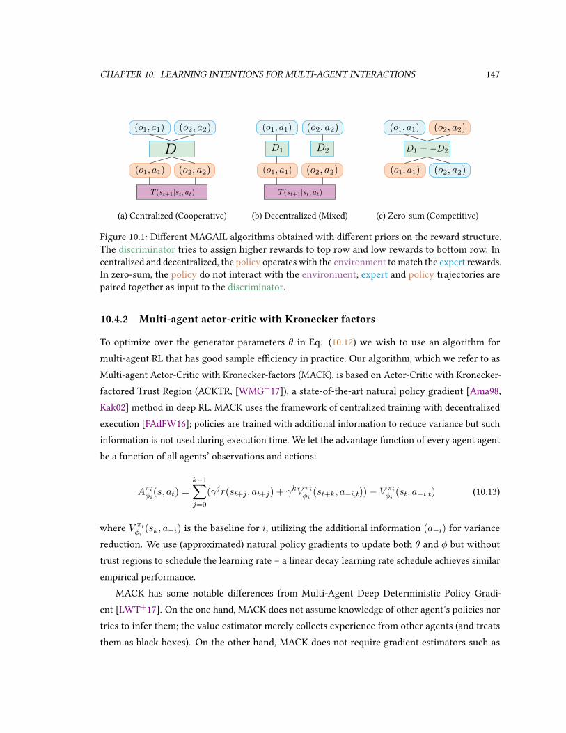
CHAPTER 10. LEARNING INTENTIONS FOR MULTI-AGENT INTERACTIONS 147
(o1, a1) (o2, a2)
(o1, a1) (o2, a2)
D
T (st+1|st, at)
(a) Centralized (Cooperative)
(o1, a1) (o2, a2)
(o1, a1) (o2, a2)
D1 D2
T (st+1|st, at)
(b) Decentralized (Mixed)
(o1, a1)
(o2, a2)(o1, a1)
(o2, a2)
D1 = −D2
(c) Zero-sum (Competitive)
Figure 10.1: Dierent MAGAIL algorithms obtained with dierent priors on the reward structure.The discriminator tries to assign higher rewards to top row and low rewards to bottom row. Incentralized and decentralized, the policy operates with the environment to match the expert rewards.In zero-sum, the policy do not interact with the environment; expert and policy trajectories arepaired together as input to the discriminator.
10.4.2 Multi-agent actor-critic with Kronecker factors
To optimize over the generator parameters θ in Eq. (10.12) we wish to use an algorithm formulti-agent RL that has good sample eciency in practice. Our algorithm, which we refer to asMulti-agent Actor-Critic with Kronecker-factors (MACK), is based on Actor-Critic with Kronecker-factored Trust Region (ACKTR, [WMG+17]), a state-of-the-art natural policy gradient [Ama98,Kak02] method in deep RL. MACK uses the framework of centralized training with decentralizedexecution [FAdFW16]; policies are trained with additional information to reduce variance but suchinformation is not used during execution time. We let the advantage function of every agent agentbe a function of all agents’ observations and actions:
Aπiφi(s, at) =
k−1∑j=0
(γjr(st+j , at+j) + γkV πiφi
(st+k, a−i,t))− V πiφi
(st, a−i,t) (10.13)
where V πiφi
(sk, a−i) is the baseline for i, utilizing the additional information (a−i) for variancereduction. We use (approximated) natural policy gradients to update both θ and φ but withouttrust regions to schedule the learning rate – a linear decay learning rate schedule achieves similarempirical performance.
MACK has some notable dierences from Multi-Agent Deep Deterministic Policy Gradi-ent [LWT+17]. On the one hand, MACK does not assume knowledge of other agent’s policies nortries to infer them; the value estimator merely collects experience from other agents (and treatsthem as black boxes). On the other hand, MACK does not require gradient estimators such as

CHAPTER 10. LEARNING INTENTIONS FOR MULTI-AGENT INTERACTIONS 148
Gumbel-softmax [JGP16] to optimize over discrete actions, which is necessary for DDPG [LHP+15].
10.5 Scaling up Multi-agent Inverse Reinforcement Learning
Accurate models of human behavior are increasingly important to safe and eective deployment ofautonomous systems. Despite this need, behavior modeling remains dicult for various commonproblem settings. Urban environments, for example, still pose signicant challenges for autonomousplanning because of the uncertainty resulting from a high density of people [SAMR18]. To describethese scenarios robustly, a model must capture multi-modality in agent motivations and complexinteractions that often scale super-linearly with the number of agents.
10.5.1 Scalable Modeling with Latent Variables
To address the scalability issue, we propose to model the policy and reward functions with latentvariables. Specically, we may assume the reward function for agent i can be modeled using alatent variable zi, and is dened as rφ(ait, st|zi) with parameters φ respectively. We further assumethat the latent variable has the prior p(z) = N (µz, σz).
With the latent variables and conditional reward model, the objective becomes:
L(φ) = Eτ∼πE
[N∑i=1
log
(∫zip(zi)
exp(∑
t rφ(ait, st|zi))Z(rφ, zi)
dzi)]
(10.14)
To remove the summation over p(zi) in the log, we introduce a inference model qω(zi|τ i), whereτ i = (sit, ait) is the trajectory for agent i. This leads to an evidence lower bound to L(φ) [KW13]:
L(φ) ≥ Eτ∼πE
[N∑i=1
Ezi∼qω(zi|τ i)[ELBOφ,ω(τ i, zi)]
](10.15)
where ELBOφ,ω(τ i, zi) is dened as:
∑t
rφ(ait, st|zi)− logZ(rφ, zi)− log qω(zi|τ i) + log p(zi) (10.16)
Given zi, we can then optimize the rst two terms in ELBOφ,ω(τ i, zi) with AIRL, which providesboth the reward function and the corresponding policy as discussed next.

CHAPTER 10. LEARNING INTENTIONS FOR MULTI-AGENT INTERACTIONS 149
10.5.2 Multi-agent AIRL with Latent Variables
We propose an Adversarial Inverse Reinforcement Learning (AIRL, [FLL17]) algorithm that maxi-mizes the evidence lower bound objective in Equation 10.16. First, for the latent variable model qω ,we introduce a inference network qω(z|τ) that predicts the latent variable from trajectories. FromEquation 10.16, this corresponds to the following objective:
Lqω = −Eτ∼πE ,z∼qω(z|τ)[log qω(z|τ)− log p(z)] (10.17)
Then, conditioned on the latent variable z, we can transform the rst term of Equation 10.16using an AIRL approach. Here we need an additional discriminator Dθ,φ(s, a, z) that depends onstate s, action a and the latent variable z, whose goal is to discriminate generated trajectories andthe demonstrations. Specically, one provides a parameterized policy πθ(a|s), and the discriminatoris denoted as:
Dθ,φ(s, a, z) =exp(rφ(s, a|z))
exp(rφ(s, a|z)) + πθ(a|s, z)(10.18)
The discriminator then minimizes the following objective:
LD =− EτE∼πE ,zE∼qω(z|τE)[logDθ,φ(s, a, zE)] (10.19)
− Eτ∼πθ(z),z∼N (0,1)[log(1−Dθ,φ(s, a, z))] (10.20)
− EτE∼πθ(zE),zE∼qω(z|τE)[log(1−Dθ,φ(s, a, zE))] (10.21)
where the rst term encourages higher Dθ,φ for demonstrations, and the second and third termencourages lowerDθ,φ for trajectories generated by the policy when the latent variables are sampledfrom p(z) or inferred from demonstrations.
The learned policy πθ(a|s, z) produces an action distribution based on the latent variableand the current state, and its primary objective is to reach higher Dθ,φ values. We use πθ(z) forthe shorthand notation for the policy πθ(a|s, z) with latent variable z. To encourage the latentvariables to be informative for generating the trajectories, we add a reconstruction loss such thattrajectories in τE could be reconstructed via qω(z|τE) (encoder) and πθ(a|s, z) (decoder), similarto InfoGAIL [LSE17a]. This leads to the objective:
LG = −Eτ∼πθ(z),z∼p(z)[Dθ,φ(s, a, z)] + EτE∼πθ(zE),zE∼qω(z|τE),τE∼πE [‖τE − τE‖2] (10.22)

CHAPTER 10. LEARNING INTENTIONS FOR MULTI-AGENT INTERACTIONS 150
These loss functions are iteratively minimized with stochastic gradient descent.
10.6 Experiments
We evaluate the performance of (centralized, decentralized, and zero-sum versions) of MAGAILunder two types of environments. One is a particle environment which allows for complex interac-tions and behaviors; the other is a control task, where multiple agents try to cooperate and move aplank forward. We collect results by averaging over 5 random seeds. Our implementation is basedon OpenAI baselines [DHK+17]; please refer to Appendix B.8.2 for implementation details.
We compare our methods (centralized, decentralized, zero-sum MAGAIL) with two baselines.The rst is behavior cloning (BC), which learns a maximum likelihood estimate for ai given eachstate s and does not require actions from other agents. The second baseline is the GAIL IRL baselinethat operates on each agent separately – for each agent we rst pretrain the other agents with BC,and then train the agent with GAIL; we then gather the trained GAIL policies from all the agentsand evaluate their performance.
10.6.1 Particle environments
We rst consider the particle environment proposed in [LWT+17], which consists of severalagents and landmarks. We consider two cooperative environments and two competitive ones. Allenvironments have an underlying true reward function that allows us to evaluate the performanceof learned agents.
The environments include: Cooperative Communication – two agents must cooperate toreach one of three colored landmarks. One agent (“speaker”) knows the goal but cannot move, so itmust convey the message to the other agent (“listener”) that moves but does not observe the goal.Cooperative Navigation – three agents must cooperate through physical actions to reach threelandmarks; ideally, each agent should cover a single landmark. Keep-Away – two agents havecontradictory goals, where agent 1 tries to reach one of the two targeted landmarks, while agent2 (the adversary) tries to keep agent 1 from reaching its target. The adversary does not observethe target, so it must act based on agent 1’s actions. Predator-Prey – three slower cooperatingadversaries must chase the faster agent in a randomly generated environment with obstacles; theadversaries are rewarded by touching the agent while the agent is penalized.
For the cooperative tasks, we use an analytic expression dening the expert policy; for thecompetitive tasks, we use MACK to train expert policies based on the true underlying rewards

CHAPTER 10. LEARNING INTENTIONS FOR MULTI-AGENT INTERACTIONS 151
100 200 300 400# Expert Demonstrations
10.96
0.90.8
0.6
0Nor
mal
ized
Rew
ards
Cooperative Communication
100 200 300 400# Expert Demonstrations
10.96
0.90.8
0.6
0
Cooperative Navigation
Expert Random BC GAIL Centralized Decentralized
Figure 10.2: Average true reward from cooperative tasks. Performance of experts and randompolicies are normalized to one and zero respectively. We use inverse log scale for better comparison.
(using larger policy and value networks than the ones that we use for imitation). We then use theexpert policies to simulate trajectories D, and then do imitation learning on D as demonstrations,where we assume the underlying rewards are unknown. Following [LSE17b], we pretrain ourMulti-Agent GAIL methods and the GAIL baseline using behavior cloning as initialization to reducesample complexity for exploration. We consider 100 to 400 episodes of expert demonstrations, eachwith 50 timesteps, which is close to the amount of timesteps used for the control tasks in [HE16].Moreover, we randomly sample the starting position of agent and landmarks each episode, so ourpolicies have to learn to generalize when they encounter new settings.
Cooperative tasks
We evaluate performance in cooperative tasks via the average expected reward obtained by all theagents in an episode. In this environment, the starting state is randomly initialized, so generalizationis crucial. We do not consider the zero-sum case, since it violates the cooperative nature of the task.We display the performance of centralized, decentralized, GAIL and BC in Figure 10.2.
Naturally, the performance of BC and MAGAIL increases with more expert demonstrations.MAGAIL performs consistently better than BC in all the settings; interestingly, in the cooperativecommunication task, centralized MAGAIL is able to achieve expert-level performance with only200 demonstrations, but BC fails to come close even with 400 trajectories. Moreover, the central-ized MAGAIL performs slightly better than decentralized MAGAIL due to the better prior, butdecentralized MAGAIL still learns a highly correlated reward between two agents.

CHAPTER 10. LEARNING INTENTIONS FOR MULTI-AGENT INTERACTIONS 152
Table 10.1: Average agent rewards in competitive tasks. We compare behavior cloning (BC), GAIL(G), Centralized (C), Decentralized (D), and Zero-Sum (ZS) methods. Best marked in bold (high vs.low rewards is preferable depending on the agent vs. adversary role).
Task Predator-PreyAgent Behavior Cloning G C D ZS
Adversary BC G C D ZS Behavior CloningRewards -93.20 -93.71 -93.75 -95.22 -95.48 -90.55 -91.36 -85.00 -89.4
Task Keep-AwayAgent Behavior Cloning G C D ZS
Adversary BC G C D ZS Behavior CloningRewards 24.22 24.04 23.28 23.56 23.19 26.22 26.61 28.73 27.80
Competitive tasks
We consider all three types of Multi-Agent GAIL (centralized, decentralized, zero-sum) and BCin both competitive tasks. Since there are two opposing sides, it is hard to measure performancedirectly. Therefore, we compare by letting (agents trained by) BC play against (adversaries trainedby) other methods, and vice versa. From Table 10.1, decentralized and zero-sum MAGAIL oftenperform better than centralized MAGAIL and BC, which suggests that the selection of the suitableprior ψ is important for good empirical performance. More details for all the particle environmentsare in the appendix.
10.6.2 Cooperative control with MA-GAIL
In some cases we are presented with sub-optimal expert demonstrations because the environmenthas changed; we consider this case in a cooperative control task [KGE17], whereN bipedal walkerscooperate to move a long plank forward; the agents have incentive to collaborate since the plank ismuch longer than any of the agents. The expert demonstrates its policy on an environment withno bumps on the ground and heavy weights, while we perform imitation in an new environmentwith bumps and lighter weights (so one is likely to use too much force). Agents trained with BCtend to act more aggressively and fail, whereas agents trained with centralized MAGAIL can adaptto the new environment. With 10 (imperfect) expert demonstrations, BC agents have a chance offailure of 39.8% (with a reward of 1.26), while centralized MAGAIL agents fail only 26.2% of thetime (with a reward of 26.57). We show videos of respective policies in the supplementary.

CHAPTER 10. LEARNING INTENTIONS FOR MULTI-AGENT INTERACTIONS 153
10.6.3 Transportation Environments
In this section, we consider multi-agent imitation learning and inverse reinforcement learning intransportation environments where scalability is crucial.
Deterministic Transition Model
In the transportation environments, we assume that the state st contains the location~l and velocities~v of all agents:
st = sit
sit =
(~lt, ~vt)i Oit = O[a]
sO else
where we consider ~l, ~v ∈ R2 for car trajectories (2d) and ~l, ~v ∈ R3 for airplane trajectories (3d).We assume that the action for each agent is to change its location and velocity (denoted as ∆~l and∆~v respectively). The extra null state sO and action aO are taken to be values far from the datadistribution such as the largest number possible in 64-bit oating point. The transition model ofalive agents is dened as
T ′((~lt+1, ~vt+1)i | (~lt, ~vt)i, (∆~l, ∆~v)it) = (~lt + (∆~l)t, ~vt + (∆~v)t)i
which is deterministic. Learning ∆~l as well as ∆~v (instead of using second order ODEs) is useful inthis case because it compensates for temporal downsampling of the data and discretization of time.
Data
HighD Dataset The HighD dataset [KBKE18] comprises over 100,000 short vehicle trajectoriesgathered from drone footage of German highways. We used the locations with 3 lanes (majority ofdataset), and preprocessed by making all velocities positive and rescaling and shifting to a sharedcoordinate system. As lane markings diered slightly due to drone camera angle, we took the truelocation to be the average across all the recordings after scaling. To aid our optimization objective,we also downsampled the trajectories without lane changes so that the resulting trajectories were30% lane changes. This prevented the highly biased dataset from biasing the generative model inthe early phases of its training. Additionally, for convenience, we aggressively downsampled the

CHAPTER 10. LEARNING INTENTIONS FOR MULTI-AGENT INTERACTIONS 154
trajectories in time, sacricing a smoother dynamics model for a smaller computational burden.As vehicles are not point particles in the HighD dataset and have lateral dimensions, we found
training could be accelerated by including the relative locations of the edges making up each of thetwo vehicle’s bounding boxes as inputs to the state encoder. Though not strictly necessary, thisproved to aid convergence.
FAA Dataset The aircraft trajectory dataset consists of tracks gathered from the Federal AviationAdministration (FAA) multi-sensor fusion tracker [JSV08]. The dataset contains six months ofights from locations in Central Florida, New York City, and Southern California, though for thiswork we only used ights to and from JFK airport in New York City. Raw tracks contain thelat long and altitude of each aircraft. These (x, y, z) points are smoothed using the optimizationprocedure described in [BKB18] and approximate velocities are calculated by temporal dierences.All trajectories are bounded at 40 km (∼25 miles) from the airport laterally and 3 km (∼10000 ft)in altitude. As with the HighD vehicle trajectories, we also temporally downsampled the aircrafttrajectories which in their raw form often had sequence lengths on the order of hundreds orthousands. In order to provide as much contextual information to the model as possible, we alsojoined trajectory data with hourly historical weather data from the NOAA, which included windspeed, wind direction, and visibility, among other features.
Results
Learned Policies We used two types of metrics to evaluated the policies learned by our models.To measure how eectively the learned distribution can cover the expert distribution, we calculatethe average and nal displacement between sampled trajectories drawn from a particular startingstate sit0 and the ground truth trajectory, holding the policies of the other agents xed as expert.The reported number is the minimum over 10 sampled latent variables. Additionally, we measure“emergent” properties of the learned policies in the setting of multi-agent control. These emergentproperties include the distribution of speeds, distance between agents, and rate of anomalous events(such as driving o the road or going to zero altitude far from the airport). For the HighD datadistance between agents is reported as distance headway (DHW)–the distance to the precedingcar in the lane if it exists–and time-to-collision (TTC) as these are the typical metrics used indriving simulation. The benchmark our models, we compare them with the policy with the LSTMremoved as well as our full model with the latent variable z removed. Results for the HighD andFAA datasets are shown in Tables 10.2 and 10.3. From these ablations, we see that the proposed

CHAPTER 10. LEARNING INTENTIONS FOR MULTI-AGENT INTERACTIONS 155
Table 10.2: Results on the HighD dataset.
HighDmetric w/o lstm & latent w/o latent w/ latent expert
avg. displacement (m) 5.89 5.03 4.93nal displacement (m) 6.57 5.68 5.61
min speed (m/s) 22.4 21.6 23.7 21.2max speed (m/s) 44.8 40.3 37.2 39.5rate bad nal state (%) 2.6 1.15 1.24 0.0avg. DHW (m) 51.3 58.2 63.8 56.7avg. TTC (s) 143 152 168 159
Table 10.3: Results on the FAA dataset.
FAAmetric w/o lstm & latent w/o latent w/ latent expert
avg. displacement (m) 823 670 596nal displacement (m) 897 808 785
min speed (m/s) 58.7 61.0 59.3 64.8max speed (m/s) 310 296 302 287rate bad nal state (%) 7.52 6.01 5.32 0.0avg. inter-agent dist. (m) 28000 26100 25200 24300
method is able to achieve low displacement from expert trajectory and emergent properties similar to
those of expert trajectories. The rate of bad nal states is perhaps the most relevant among theseemergent properties and this is minimal with the full model on both datasets.
As the learned latent variables are a focus of this work, we show visualizations of rolloutswhere latent variables are drawn from across the distribution. Figure 10.3 shows a distribution ofhighway driving trajectories. This visualization illustrates the primary role of the latent variablefor the HighD dataset is modeling lane-changing behavior. Figure 10.4 shows a distribution oftakeo trajectories out of JFK airport. Here we see the latent variable captures the shape of thetrajectory, which contains information about direction and altitude changes3.
Learned Reward Functions
Verifying learned reward function in an IRL setting is challenging in general. In our setting, the3Video demonstrations of our learned policies in http://bit.ly/multi-agent-trac.

CHAPTER 10. LEARNING INTENTIONS FOR MULTI-AGENT INTERACTIONS 156
Figure 10.3: Expert trajectories are shown in green while a rollout for one value of z is shown inred. A full distribution of positions from trajectories resulting from many z ∼ N (0, 1) are shownas a density. The latent variable primarily captures the driver’s willingness to change lanes, withconcentrations of density moving out to the adjacent lanes as well as behind the preceding car.Agents further away from the rolled out agent are not shown for visual clarity.
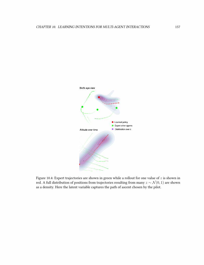
CHAPTER 10. LEARNING INTENTIONS FOR MULTI-AGENT INTERACTIONS 157
Figure 10.4: Expert trajectories are shown in green while a rollout for one value of z is shown inred. A full distribution of positions from trajectories resulting from many z ∼ N (0, 1) are shownas a density. Here the latent variable captures the path of ascent chosen by the pilot.

CHAPTER 10. LEARNING INTENTIONS FOR MULTI-AGENT INTERACTIONS 158
Figure 10.5: Visualization of a learned reward function when the state of the vehicle is rolledforward in time. Cars appear closer horizontally than they are in real life, as the true aspect ratioof the road is much higher.
challenge remains because we do not have access to any ground truth rewards. Luckily, however,visualization in this setting is feasible and human intuition can be used for qualitatively validatingthe rewards. We visualize learned rewards by plotting the distribution of rewards around a vehicle.Specically, we calculate the rewards over a grid of possible locations surrounding the vehicle,leaving the locations of the other vehicles xed. Rewards are normalized between zero and oneand the resulting density is smoothed with a Gaussian kernel.
Figure 10.5 shows two visualizations of reward functions learned from the HighD dataset. Bothreward functions reect a lane-change objective–one in less congestion and another in a higherlevel of congestion where rewards are more aected by the locations of other agents. Figure 10.6shows a learned reward function on the FAA dataset. We see a similar reward function that reectsnear-term navigational goals. In general, reward functions learned from the FAA dataset show lessdramatic dependence on other agents, as we would expect given the implicit eect of terminal airtrac control.
10.7 Related work and discussion
There is a vast literature on single-agent imitation learning [Bag15]. Behavior Cloning (BC)learns the policy through supervised learning [Pom91]. Inverse Reinforcement Learning (IRL)assumes the expert policy optimizes over some unknown reward, recovers the reward, and learnsthe policy through reinforcement learning (RL). BC does not require knowledge of transitionprobabilities or access to the environment, but suers from compounding errors and covariateshift [RAB10, RGB11].

CHAPTER 10. LEARNING INTENTIONS FOR MULTI-AGENT INTERACTIONS 159
Figure 10.6: Visualization of reward function learned from the FAA dataset. Rewards are clearlycorrelated with the ight path of the pilot, in this case a looping ascent to the NE.

CHAPTER 10. LEARNING INTENTIONS FOR MULTI-AGENT INTERACTIONS 160
Most existing work in multi-agent imitation learning assumes the agents have very specicreward structures. The most common case is fully cooperative agents, where the challengesmainly lie in other factors, such as unknown role assignments [LYC17], scalability to swarmsystems [ŠKZK16] and agents with partial observations [BD14]. In non-cooperative settings,[LBC14] consider the case of IRL for two-player zero-sum games and cast the IRL problem asBayesian inference, while [RGZH12] assume agents are non-cooperative but the reward function isa linear combination of pre-specied features.
The use of latent variables to learn multi-modal policies have been considered in single agentimitation learning, such as learning multi-modal policies [LSE17a] or meta-learning [YYFE19]. Ourapproach makes two distinctions from these previous ones: dierent from [LSE17a], our latentvariables are continuous since there is no explicit prior about the number of dierent policies;dierent from [YYFE19], we assume a prior distribution on the latent variable so as to generatenew policies unconditionally. These dierences allow us to generate diverse multi-agent behaviorswithin the same environment; using latent variables would also decrease sample complexity asopposed to learning the policy of each agent separately.
Experimental results demonstrate that our methods are able to imitate complex behaviorsand learn suitable reward functions in high-dimensional environments with both cooperativeand adversarial interactions. An interesting research direction is to explore new techniques forgathering expert demonstration; for example, when the expert is allowed to aid the agents byparticipating in part of the agent’s learning process [HMRAD16].

Chapter 11
Conclusions
11.1 Summary of Contributions
The motivating theme of this dissertation was to develop articial intelligence (AI) agents thatadapts to our various needs in complex, high-dimensional, non-stationary, real-world environments.In particular, we focus on machine learning (ML)-based AI systems that leverages data, models andcomputational systems. A key challenge in current ML systems is the need for supervision, whichdoes not apply well to cases where supervision signals are dicult to capture – these cases includecompression, generation, and inference. To address the unique problems in these scenarios, wedeveloped theory and algorithms that applies supervised learning techniques and implementedsolutions to various application domains. In the following, we summarize the contribution withineach of these parts.
In Part I, we discuss the problem of compression (unsupervised representation learning) andframe the problem within the context of variational mutual information estimation / maximization.We start by analyzing variational mutual information objectives for representation learning, discusstheir limitations, and introduce a low-variance estimator of mutual information (Chapter 2). Wethen follow up by introducing an estimator based on multi-label classication that can also beoptimized eciently for representation learning (Chapter 3). Finally, we apply the above ideas andconsider information-theoretical approaches to learning fair representations, which uses regressionto estimate and optimize mutual information (Chapter 4). These approaches have been applied tolearning informative and fair representations from data.
In Part II, we discuss how supervised learning can be advanced for generation, i.e., learninghigh-dimensional probabilistic models of data (generation). First, we start by improving generative
161

CHAPTER 11. CONCLUSIONS 162
adversarial networks (GANs) by reweighting the supervised learning objective. We proposed aunied objective for f -GANs and Wasserstein GANs, which allows us to interpret them as objectivefunctions that can be reweighted for better generative modeling performance. Next, we improveGANs by introducing a novel negative data augmentation technique. This introduces negativesamples into the supervised learning procedure of training GANs, and is able to encourage GANdiscriminators to capture additional global information of the data. Negative data augmentationcan also be used the compression algorithms that we discussed in Part I. Finally, we discuss howwe can incorporate compression techniques from the previous part to enable few-shot conditionalgeneration capabilities of generative models. We introduced an ecient sampling procedure fordiusion generative models, applied it to the latent space of variational autoencoders, which allowsus to learn high-delity generative models with informative latent spaces. Such a latent space canbe used for various few-shot conditional generation tasks, such as conditional image generationand image manipulation.
In Part III we discuss how supervised learning can be used to improve probabilistic inferencemethods. In Chapter 8, we discuss how supervised learning is used to automate design choicesin Bayesian inference that were previously hand-designed. We replace hand-designed heuristicswith automated supervised learning algorithms, allowing us to vastly improve the eciency ofBayesian inference algorithms. In Chapter 9, we apply supervised learning to multi-agent imitationlearning and inverse reinforcement learning, where machines can imitate the behavior of real-worldmulti-agent demonstrations while learning exible reward functions from them. We demonstratedour methods on a range of environments, such as cooperative robotic control, road trac, and airtrac.
11.2 Future Work
The contributions of this dissertation suggest new opportunities and challenges for future work,some of which we highlight below.
Flexible, hierarchical representation learning In representation learning, the optimal levelof abstraction is task-dependent: information about color and texture is crucial if our goal is toreproduce an image, but much less so if our goal is to merely recognize objects. Most existingworks on unsupervised representation learning only have a single level of abstraction that is“biased” towards certain tasks, limiting the ability to adapt to novel ones. I believe that the next

CHAPTER 11. CONCLUSIONS 163
generation of intelligent systems learning from real-world data should form a exible hierarchyof abstractions that is suited to more general tasks and adapt them to novel tasks. Having moreexibility in the representations also opens up the possibility to incorporate structured domainknowledge, which we have explored in the context of structured prediction [RSS+18]. Learningexible representations can also lead to new computational tools that can facilitate applicationareas where high quality supervision is scarce, such as generative modeling, scientic discovery,and computational sustainability.
Generative modeling with conditions As intelligent systems grow increasingly complicated,interpreting them becomes more challenging, so it is crucial for these systems to be able torepresent their knowledge in more interpretable ways, such as images, text, or graphs. Thesegenerative models should also produce high-dimensional signals conditioned on our In recentworks, I explored new paradigms to training deep neural networks that accurately and ecientlymodel high-dimensional data from few-shot conditions (Chapter 8). Combining this with otherhigh-delity generative models can allow humans to better understand the model and providemore accurate feedback. This also includes pressing concerns in using generative models for fairgenerative modeling, as we show in Chapter 5 and hopefully will extend to conditional few-shotgeneration in future research.
Data-driven sequential decision making Much practical progress in machine learning overthe past few years have been driven by advances in large-scale datasets. However, in sequentialdecision making problems with human interactions (e.g., autonomous driving and dialog systems),accurate real-world data are often costly, and cheaper sources of data (e.g., simulators) are ofteninaccurate. Bridging the gap between these two sources of data could benet real-world problemsthat are dicult to describe with human labels; this requires breakthroughs in many relevantelds such as causal inference, uncertainty quantication, generative modeling, and domain adap-tation. One example is our work on re-calibration techniques for model-based reinforcementlearning [MKS+19], which improves policy learning through models that better quantify uncer-tainty. I believe that we can learn from precise yet expensive real-world data to better teach ourmodels under massive, cheap sources of data, and make progress in many real-world domainswhere machines interact with humans.

Appendix A
Proofs
A.1 Proofs for Chapter 3
A.1.1 Proofs in Section 3.3
Theorem 1. ∀P,Q ∈ P(X ) such that P Q we have
DKL(P‖Q) = supr∈∆(Q)
EP [log r] (3.6)
where the supremum is achived when r = dP/ dQ.
Proof. For every T ∈ L∞(Q), dene rT = eT
EQ[eT ], then rT ∈ ∆(Q) and from the Donsker-
Varadhan inequality [DV75]
DKL(P‖Q) = supT∈L∞(Q)
EP [T ]− logEQ[eT ] (A.1)
= supT∈L∞(Q)
EP[log
eT
EQ[eT ]
]= sup
rT∈∆(Q)EP [log rT ] (A.2)
Moreover, we have:
DKL(P‖Q) = EP [log dP − log dQ] = EP[log
dP
dQ
](A.3)
which completes the proof.
164

APPENDIX A. PROOFS 165
Corollary 7. ∀P,Q ∈ P(X ) such that P Q, ∀fθ : X → R≥0 we have
I(X;Y ) ≥ ICPC(fθ) := EPn(X,Y )
[1
n
n∑i=1
logfθ(xi,yi)
1n
∑nj=1 fθ(xi,yj)
](A.4)
Proof.
nICPC(fθ) := EPn(X,Y )
[n∑i=1
logfθ(xi,yi)
1n
∑nj=1 fθ(xi,yj)
](A.5)
= EPn(X,Y )
[n∑i=1
lognfθ(xi,yi)∑nj=1 fθ(xi,yj)
](A.6)
Since
EP (X)Pn(Y )
[nfθ(x,y)∑nj=1 fθ(x,yj)
]= 1, (A.7)
we can apply Theorem 1 to obtain:
nICPC(fθ) = EPn(X,Y )
[n∑i=1
lognfθ(xi,yi)∑nj=1 fθ(xi,yj)
](A.8)
=n∑i=1
EP (Xi,Y n1 )
[log
nfθ(xi,yi)∑nj=1 fθ(xi,yj)
](A.9)
≤n∑i=1
I(Xi;Yn
1 ) = nI(X;Y ) (A.10)
where Y n1 denotes the concatenation of n independent random variables (Y1, . . . , Yn) and
P (Xi, Yn
1 ) = P (Xi, Yi)P (Y i−11 )P (Y n
i+1)
is the joint distribution of P (Xi, Yn
1 ).
A.1.2 Proofs in Section 3.4
Theorem 2. Assume that the ground truth density ratio r? = dP/ dQ and VarQ[r?] exist. Let Qndenote the empirical distribution of n i.i.d. samples from Q and let EQn denote the sample average

APPENDIX A. PROOFS 166
over Qn. Then under the randomness of the sampling procedure, we have:
VarQ[EQn [r?]] ≥ eDKL(P‖Q) − 1
n(3.10)
limn→∞
nVarQ[logEQn [r?]] ≥ eDKL(P‖Q) − 1. (3.11)
Proof. Consider the variance of r?(x) when x ∼ Q:
VarQ[r?] = EQ
[(dP
dQ
)2]−(EQ[
dP
dQ
])2
(A.11)
= EP[
dP
dQ
]− 1 (A.12)
≥ eEP [log dPdQ
] − 1 (A.13)
= eDKL(P‖Q) − 1 (A.14)
where (A.11) uses the denition of variance, (A.12) uses the denition of Radon-Nikodym derivativeto change measures, (A.13) uses Jensen’s inequality over log, and (A.14) uses the denition of KLdivergences.
The variance of the mean of n i.i.d. random variables then gives us:
VarQ[EQn [r]] =Var[r]
n≥ eDKL(P‖Q) − 1
n(A.15)
which is the rst part of the theorem.As n→∞, VarQ[EQn [r]]→ 0, so we can apply the delta method:
VarQ[f(X)] ≈ (f ′(E(X)))2 VarQ[X] (A.16)
Applying f = log and E[X] = 1 gives us the second part of the theorem:
limn→∞
nVarQ[logEQn [r]] = limn→∞
nVar[EQn [r]] ≥ eDKL(P‖Q) − 1 (A.17)
which describes the variance in the asymptotic sense.
Corollary 1. Assume that the assumptions in Theorem 2 hold. Let Pm and Qn be the empirical

APPENDIX A. PROOFS 167
distributions ofm i.i.d. samples from P and n i.i.d. samples from Q, respectively. Dene
Im,nNWJ := EPm [log r? + 1]− EQn [r?] (3.12)
Im,nMINE := EPm [log r?]− logEQn [r?] (3.13)
where r? = dP/dQ. Then under the randomness of the sampling procedure, we have ∀m ∈ N:
VarP,Q[Im,nNWJ] ≥ (eDKL(P‖Q) − 1)/n (3.14)
limn→∞
nVarP,Q[Im,nMINE] ≥ eDKL(P‖Q) − 1. (3.15)
Proof. Since Pm and Qn are independent, we have
Var[Im,nNWJ] ≥ Var[EQn [r?]] (A.18)
= Var[EQn [r?]] ≥ eDKL(P‖Q) − 1
n(A.19)
and
limn→∞
nVar[Im,nMINE] ≥ limn→∞
nVar[logEQn [r?]] ≥ eDKL(P‖Q) − 1 (A.20)
which completes the proof.
A.1.3 Proofs in Section 3.5
Theorem 3. Let r(x) : X → R≥0 be any non-negative measurable function such that∫rdQ = S,
S ∈ (0,∞) and r(x) ∈ [0, eK ]. Dene rτ (x) = clip(r(x), eτ , e−τ ) for nite, non-negative τ . If
τ < K , then the bias for using rτ to estimate the partition function of r satises:
|EQ[r]− EQ[rτ ]| ≤ max
(e−τ |1− Se−τ |,
∣∣∣∣1− eKe−τ + S(eK − eτ )
eK − e−τ∣∣∣∣) ;
if τ ≥ K , then
|EQ[r]− EQ[rτ ]| ≤ e−τ (1− Se−K).
Proof. We establish the upper bounds by nding a worst case r to nd the largest |EQ[r]−EQ[rτ ]|.First, without loss of generality, we may assume that r(x) ∈ (−∞, e−τ ] ∪ [eτ ,∞) for all x ∈ X .
APPENDIX A. PROOFS 168
Otherwise, denote Xτ (r) = x ∈ X : e−τ < r(x) < eτ as the (measurable) set where the r(x)
values are between e−τ and eτ . Let
Vτ (r) =
∫x∈Xτ (r)
r(x)dx ∈ (e−τ |Xτ (r)|, eτ |Xτ (r)|) (A.21)
be the integral of r over Xτ (r). We can transform r(x) for all x ∈ Xτ (r) to have values only ine−τ , eτ and still integrate to Vτ (r), so the expectation under Q is not changed.
Then we show that we can rescale all the values above eτ and below eτ to the same valuewithout changing the expected value under Q. We denote
K1 = log
∫I(r(x) ≤ e−τ )r(x)dQ(x)− log
∫I(r(x) ≤ e−τ )dQ(x) (A.22)
K2 = log
∫I(r(x) ≥ eτ )r(x)dQ(x)− log
∫I(r(x) ≥ eτ )dQ(x) (A.23)
where eK1 and eK2 represents the mean of r(x) for all r(x) ≤ e−τ and r(x) ≥ eτ respectively.We then have:
EQ[r] = eK1
∫I(r(x) ≤ e−τ )dQ(x) + eK2
∫I(r(x) ≥ eτ )dQ(x) (A.24)
1 =
∫I(r(x) ≤ e−τ )dQ(x) +
∫I(r(x) ≥ eτ )dQ(x) (A.25)
so we can parametrize EQ[r] via K1 and K2. Since EQ[r] = S by assumption, we have:
∫I(r(x) ≤ e−τ )dQ(x) =
eK2 − SeK2 − e−K1
(A.26)
and from the denition of rτ (x):
EQ[rτ ] =eK2e−τ − Se−τ + Seτ − e−K1eτ
eK2 − e−K1:= g(K1,K2) (A.27)
We can obtain an upper bound once we nd max g(K1,K2) and min g(K1,K2). First, we have:
∂g(K1,K2)
∂K1=e−K1eτ (eK2 − e−K1)− e−K1(eK2e−τ − Se−τ + Seτ − e−K1eτ )
(eK2 − e−K1)2
=e−K1(eτ − e−τ )(eK2 − S)
(eK2 − e−K1)2≥ 0 (A.28)

APPENDIX A. PROOFS 169
∂g(K1,K2)
∂K2=eK2e−τ (eK2 − e−K1)− eK2(eK2e−τ − Se−τ + Seτ − e−K1eτ )
(eK2 − e−K1)2
=eK2(eτ − e−τ )(e−K1 − S)
(eK2 − e−K1)2≤ 0 (A.29)
Therefore, g(K1,K2) is largest when K1 →∞,K2 = τ and smallest when K1 = τ,K2 →∞.
max g(K1,K2) = limK→∞
1− e−Keτ + S(eτ − e−τ )
eτ − e−K = S + e−τ − Se−2τ (A.30)
min g(K1,K2) = limK→∞
eKe−τ − 1 + S(eτ − e−τ )
eK − e−τ = e−τ (A.31)
Therefore,
|EQ[r]− EQ[rτ ]| ≤ max(|max g(K1,K2)− S|, |S −min g(K1,K2)|) (A.32)
= max(|e−τ − Se−2τ |, |S − e−τ |
)(A.33)
The proof for Theorem 3 simply follows the above analysis for xed K . When τ < K , weconsider the case when K1 →∞,K2 = τ and K1 = τ,K2 = K; when τ > K only the smallervalues will be clipped, so the increased value is no larger than the case where K1 →∞,K2 = K :
eK − SeK
· eτ = e−τ (1− Se−K) (A.34)
where eK ≥ S from the fact that∫r dQ = S.
Theorem 4. The variance of the estimator EQn [rτ ] (using n samples from Q) satises:
Var[EQn [rτ ]] ≤ eτ − e−τ4n
(3.18)
Proof. Since rτ (x) is bounded between eτ and e−τ , we have
Var[rτ ] ≤ eτ − e−τ4
(A.35)
Taking the mean of n independent random variables gives us the result.
Combining Theorem 3 and 4 with the bias-variance trade-o argument, we have the following:

APPENDIX A. PROOFS 170
Corollary 8. Let r(x) : X → R≥0 be any non-negative measurable function such that∫rdQ = S,
S ∈ (0,∞) and r(x) ∈ [0, eK ]. Dene rτ (x) = clip(r(x), eτ , e−τ ) for nite, non-negative τ and
EQn as the sample average of n i.i.d. samples from Q. If τ < K , then
EQ[(r − EQn [rτ ])2] ≤ max
(e−τ |1− Se−τ |,
∣∣∣∣1− eKe−τ + S(eK − eτ )
eK − e−τ∣∣∣∣)2
+eτ − e−τ
4n;
If τ ≥ K , then:
EQ[(r − EQn [rτ ])2] ≤ e−2τ (1− Se−K)2 +eτ − e−τ
4n(A.36)
A.2 Proofs for Chapter 4
A.2.1 Preliminary Lemma and Propositions
To prove the main results, we need the following Lemma and Propositions 6 and 7. The Lemma is aspecial case to the dual representation of f -divergences discussed in [NWJ08].
Lemma 9 (Nguyen et al. [NWJ08]). ∀P,Q ∈ P(X ) such that P Q,
DKL(P‖Q) = supT∈L∞(Q)
EP [T ]− EQ[eT ] + 1 (A.37)
Proof. (Sketch) Please refer to [NWJ08] for a more formal proof.Denote f(t) = t log t whose convex conjugate is f?(u) = exp(u− 1), we have that
DKL(P‖Q) = Ex∼Q[f
(dP
dQ(x)
)]= Ex∼Q
[supuu · dP
dQ(x)− f?(u)
](A.38)
= supT∈L∞(Q)
Ex∼Q[T (x) · dP
dQ(x)− f?(T (x))
](A.39)
= supT∈L∞(Q)
Ex∼P [T (x)]− Ex∼Q [f?(T (x))] (A.40)
= supT∈L∞(Q)
Ex∼P [T (x) + 1]− Ex∼Q [exp(T (x))] , (A.41)
which completes the proof.
Proposition 6. For all positive integers n ≥ 1,m ≥ 2, and for any collection of positive random
variables Xini=1, Xi,jmj=1 such that ∀i ∈ [n], Xi, Xi,1, Xi,2, . . . , Xi,m−1 are exchangeable, then

APPENDIX A. PROOFS 171
∀α ∈ (0, 2mm+1 ], the following is true:
E
[1
n
n∑i=1
mXi
αXi + m−αm−1
∑m−1j=1 Xi,j
]≤ 1
α. (A.42)
Proof. First, for α ∈ (0, 2m/(m+ 1)] we have:
nE
[1
n
n∑i=1
mXi
αXi + m−αm−1
∑m−1j=1 Xi,j
](A.43)
= E
n∑i=1
mm−1m−αXi
(Σi)−(
1− m−1m−αα
)Xi
(A.44)
= E
[n∑i=1
mm−1m−α
Σi/Xi − (1− m−1m−αα)
](A.45)
= mm− 1
m− αE
n∑i=1
∞∑p=0
(Xi
Σi
)p+1(1− m− 1
m− αα)p (Taylor expansion) (A.46)
= mm− 1
m− αn∑i=1
∞∑p=0
E
[(Xi
Σi
)p+1](
1− m− 1
m− αα)p
(A.47)
where we simplify the notation with Σi := Xi +∑m−1
j=1 Xi,j . Furthermore, we note that the Taylorseries converges because (1− m−1
m−αα) ∈ (−1, 1).Since the random variables are exchangeable, switching the ordering of Xi, Xi,1, . . . , Xi,m−1
does not aect the joint distribution, and the summing function is permutation invariant. Therefore,for all i ∈ [n], p ≥ 0,
E
[(Xi
Σi
)p+1]
=1
mE
(Xi
Σi
)p+1
+m−1∑j=1
(Xi,j
Σi
)p+1 (A.48)
≤ 1
mE
Xi
Σi+
m−1∑j=1
Xi,j
Σi
p+1 =1
m(A.49)
where the last inequality comes from the fact that(Xi +
∑m−1j=1 Xi,j
)/Σi = 1 and all the random

APPENDIX A. PROOFS 172
variables are positive. Continuing from equation A.47, we have:
nE
[1
n
n∑i=1
mXi
αXi + m−αm−1
∑m−1j=1 Xi,j
](A.50)
≤ nmm− 1
m− α∞∑p=0
1
m
(1− m− 1
m− αα)p
=m− 1
m− αn
αm−1m−α
=n
α(A.51)
Dividing both sides by n completes the proof for α ∈ (0, 2mm+1 ].
Proposition 7. ∀n ≥ 1,m ≥ 2, and for any collection of positive random variables Xini=1,
Xi,jmj=1 such that ∀i ∈ [n], Xi, Xi,1, Xi,2, . . . , Xi,m−1 are exchangeable, then ∀α ∈ [1, m2 ],
E
[1
n
n∑i=1
mXi
αXi + m−αm−1
∑m−1j=1 Xi,j
]≤ 1 (A.52)
Proof. The case for α ∈ [1, 2mm+1 ] is apparent from Proposition 6.
For α ∈ (2m/(m+ 1),m/2], we have for all t ∈ [m− 1]:
E
[1
n
n∑i=1
mXi
αXi + m−αm−1
∑m−1j=1 Xi,j
](A.53)
≤ E
1
n
1
m− 1
n∑i=1
m−1∑j=1
mXi
αXi +∑j+t−1
k=j Xi,k
(A.54)
= E
1
n
1
m− 1
n∑i=1
m−1∑j=1
tXi
tαmXi +
t− tαm
t−1
∑j+t−1k=j Xi,k
(A.55)
where we deneXi,k = Xi,k−(m−1) when k > (m−1) and use the concavity of the inverse function(or equivalently the HM-AM inequality) to establish equation A.54. For anyα ∈ (2m/(m+1),m/2],we can choose t to be any integer from the interval [mα ,
2mα − 1]; we note that such an integer
always exists because the length of the interval is greater or equal to 1:
2m
α− 1− m
α=m
α− 1 ≥ 1
Then we can apply the result in Proposition 6, for t samples and the new α being tαm ; from our

APPENDIX A. PROOFS 173
construction of t, this satises the condition in Proposition 6 that:
1 ≤ tα
m≤ 2t
t+ 1
Therefore we can apply Proposition 6 to a valid choice of t to obtain
E
[1
n
n∑i=1
mXi
αXi + m−αm−1
∑m−1j=1 Xi,j
]
≤ E
1
n
1
m− 1
n∑i=1
m−1∑j=1
tXi
tαmXi +
t− tαm
t−1
∑j+t−1k=j Xi,k
≤ m
tα≤ 1
which proves the result.
A.2.2 Proof for CPC
Theorem 5. For all probability measures P,Q over sample space X such that P Q, the following
holds for all functions r : X → R+ and integersm ≥ 2:
DKL(P‖Q) ≥ Ex∼P,y1:m−1∼Qm−1
[log
m · r(x)
r(x) +∑m−1
i=1 r(yi)
]. (4.1)
Proof. From Lemma 9, we have that:
DKL(P‖Q) (A.56)
≥ Ey1:m−1∼Qm−1
[Ex∼P
[log
m · r(x)
r(x) +∑m−1
i=1 r(yi)
]− Ex∼Q
[m · r(x)
r(x) +∑m−1
i=1 r(yi)
]+ 1
]
≥ Ey1:m−1∼Qm−1
[Ex∼P
[log
m · r(x)
r(x) +∑m−1
i=1 r(yi)
]]− 1 + 1 (A.57)
= Ex∼P,y1:m−1∼Qm−1
[log
m · r(x)
r(x) +∑m−1
i=1 r(yi)
], (A.58)
where the second inequality comes from Proposition 6 where x ∼ Q and y1:m−1 ∼ Qm−1 areexchangeable, thus proving the statement.

APPENDIX A. PROOFS 174
A.2.3 Proof for ML-CPC
Theorem 6. For all probability measures P,Q over sample space X such that P Q, the following
holds for all functions r : X → R+, integers n ≥ 1,m ≥ 2, and real numbers α ∈ [ mn(m−1)+1 , 1]:
DKL(P‖Q) ≥ Ex1:n∼Pn,yi,1:m−1∼Qm−1
[1
n
n∑i=1
logmn · r(xi)
α∑n
j=1 r(xj) + m−αm−1
∑m−1k=1 r(yj,k)
].
(4.5)
Proof. First, we have
E
[1
n
n∑i=1
lognm · r(xi)
α∑n
j=1 r(xj) + m−αm−1
∑nj=1
∑m−1k=1 r(yj,k)
](A.59)
= E
[1
n
n∑i=1
log(nm · r(xi))− log
α n∑j=1
r(xj) +m− αm− 1
n∑j=1
m−1∑k=1
r(yj,k)
]
≤ E
[1
n
n∑i=1
log(nm · r(xi))− log
nαr(xi) +m− αm− 1
n∑j=1
m−1∑k=1
r(yj,k)
] (A.60)
= E
[1
n
n∑i=1
nm · r(xi)nαr(xi) + m−α
m−1
∑nj=1
∑m−1k=1 r(yj,k)
](A.61)
≤ DKL(P‖Q)− 1 + Ex1:n∼Qn
[1
n
n∑i=1
nm · r(xi)nαr(xi) + m−α
m−1
∑nj=1
∑m−1k=1 r(yj,k)
](A.62)
where we use Jensen’s inequality over log in equation A.60 and Lemma 9 in equation A.62.Since xi ∼ Q and all the yj,k are (n(m− 1) + 1) exchangeable random variables, and
m ≥ 2, α ∈[
m
n(m− 1) + 1, 1
]⇒ n(m− 1) + 1
mα ∈
[1,n(m− 1) + 1
2
],
we can apply Proposition 7 to the (n(m− 1) + 1) exchangeable variables
Ex1:n∼Qn
[1
n
n∑i=1
nm · r(xi)nαr(xi) + m−α
m−1
∑nj=1
∑m−1k=1 r(yj,k)
]
= Ex1:n∼Qn
[1
n
n∑i=1
(n(m− 1) + 1) · r(xi)n(m−1)+1
m αr(xi) +m−n(m−1)+1
nmα
m−1
∑nj=1
∑m−1k=1 r(yj,k)
]≤ 1

APPENDIX A. PROOFS 175
Combining the above with equation A.62, proves the result for the given range of α.
A.3 Proofs for Chapter 5
A.3.1 Proof of Lemma 6
Proof.
Iq(x; z|u) = Eqφ(x,z,u)[log qφ(x, z|u)− log q(x|u)− log qφ(z|u)]
= Eqφ(x,z,u)[log qφ(x, z|u)− log qφ(z|u)] + Eqφ(z,u)[− log q(x|u)]
= Eqφ(x,z,u)[log qφ(x|z,u)] +Hq(x|u)
= Eqφ(x,z,u)[log qφ(x|z,u) + log p(x|z,u)− log p(x|z,u)] +Hq(x|u)
= Eqφ(x,z,u)[log p(x|z,u)] +Hq(x|u) + Eqφ(z,u)DKL(qφ(x|z,u)‖p(x|z,u))
≥ Eqφ(x,z,u)[log p(x|z,u)] +Hq(x|u)
where the last inequality holds because KL divergence is non-negative.
A.3.2 Proof of Lemma 7
Proof.
Iq(z;u) ≤ Iq(z;x,u)
= Eqφ(x,z,u)[log qφ(z|x,u)− log qφ(z)]
= Eqφ(x,z,u)[log qφ(z|x,u)− log p(z)− log qφ(z) + log p(z)]
= Eq(x,u)DKL(qφ(z|x,u)‖p(z))−DKL(qφ(z)‖p(z))
A.3.3 Proof of Lemma 8
Proof.
Iq(z;u) = Eqφ(z,u)[log qφ(u|z)− log q(u)]
= Eqφ(z,u)[log qφ(u|z)− log p(u)− log q(u) + log p(u)]

APPENDIX A. PROOFS 176
= Eqφ(z)DKL(qφ(u|z)‖p(u))−DKL(q(u)‖p(u))
≤ Eqφ(z)DKL(qφ(u|z)‖p(u))
Again, the last inequality holds because KL divergence is non-negative.
A.3.4 Proof of Theorem 7
Proof. Let us rst verify that this problem is convex.
• Primal: −Eqφ(x,z,u)[log pθ(x|z,u)] is ane in qφ(z|x,u), convex in pθ(x|z,u) due to theconcavity of log, and independent of pθ(z).
• First condition: Eq(u)DKL(qφ(z|x,u)‖pθ(z)) is convex in qφ(z|x,u) and pθ(z) (because ofconvexity of KL-divergence), and independent of pθ(x|z,u).
• Second condition: since Eqφ(z)DKL(qφ(u|z)‖p(u))−DKL(q(u)‖p(u)) = Iq(z;u) and
Iq(z;u) = DKL(qφ(z,u)‖q(u)qφ(z)) (A.63)
= DKL(∑x
qφ(z|x,u)q(x,u)‖q(u)∑x,u
qφ(z|x,u)q(x,u)) (A.64)
Let q = βq1 + (1− β)q2, ∀β ∈ [0, 1], q1, q2. We have
Iq(z;u) = DKL(∑x
q(z|x,u)q(x,u)‖q(u)∑x,u
q(z|x,u)q(x,u))
≥ βDKL(∑x
q1(z|x,u)q(x,u)‖q(u)∑x,u
q1(z|x,u)q(x,u))
+ (1− β)DKL(∑x
q2(z|x,u)q(x,u)‖q(u)∑x,u
q2(z|x,u)q(x,u))
= βIq1(z;u) + (1− β)Iq2(z;u)
where we use the convexity of KL divergence in the inequality. Since DKL(q(u)‖p(u))
is independent of qφ(z|x,u), both Iq(z;u) and Eqφ(z)DKL(qφ(u|z)‖p(u)) are convex inqφ(z|x,u).
Then we show that the problem has a feasible solution by construction. In fact, we can simply letqφ(z|x,u) = pθ(z) be some xed distribution over z, and pθ(x|z,u) = qφ(x|z,u) for all x,u. Inthis case, z and u are independent, so DKL(qφ(z|x,u)‖pθ(z)) = 0 < ε1, DKL(qφ(u|z)‖p(u)) =

APPENDIX A. PROOFS 177
0 < ε2. This corresponds to the case where z is simply random noise that does not capture anythingin u.
Hence, Slater’s condition holds, which is a sucient condition for strong duality.
A.4 Proofs for Chapter 6
Proposition 3. ∀P,Q ∈ P(X ) such that P Q, ∀T ∈ L∞(Q) such that im(T ) ⊆ dom((f ′)−1),
and ∀R ⊆ L∞≥0(Q) such that 1 ⊆ R we have:
If (T ;P,Q) ≤ LRf (T ;P,Q) ≤ IW (T ;P,Q). (6.15)
Proof. From Propositions 1, and thatR ⊆ L∞≥0(Q), we have:
If (T ;P,Q) = infr∈L∞≥0(Q)
`f (T, r;P,Q) ≤ infr∈R
`f (T, r;P,Q) = LRf (T ;P,Q). (A.65)
From Proposition 2 and that 1 ⊆ R, we have:
LRf (T ;P,Q) = infr∈R
`f (T, r;P,Q) ≤ infr∈1
`f (T, r;P,Q) = LRf (T ;P,Q) ≤ IW (T ;P,Q). (A.66)
Combining the two inequalities completes the proof.
Theorem 8. For 1 ⊆ R ⊆ L∞≥0(Q), dene
Df,R(P‖Q) := supT∈FLRf (T ;P,Q) (6.16)
where F := T : X → dom((f ′)−1), T ∈ L∞(Q). Then
Df (P‖Q) ≤ Df,R(P‖Q) ≤ supT∈F
IW (T ;P,Q). (6.17)
Proof. From Proposition 1, we have the following upper bound for Df,R(P‖Q):
supT∈F
infr∈R
EP [f(r)] + EP [T ]− EQ[r · T ] (A.67)
≤ supT∈F
infr∈1
EP [f(r)] + EP [T ]− EQ[r · T ]
= supT∈F
EP [T ]− EQ[T ] = IPMF (P,Q),

APPENDIX A. PROOFS 178
We also have the following lower bound for Df,R(P‖Q):
supT∈F
infr∈R
EP [f(r)] + EP [T ]− EQ[r · T ] (A.68)
≥ supT∈F
infr∈L∞≥0(Q)
EP [f(r)] + EP [T ]− EQ[r · T ]
= supT∈F
EP [T ]− EQ[f∗(T )] = Df (P‖Q).
Therefore, Df,R(P‖Q) is bounded between Df (P‖Q) and IPMF (P,Q) and thus it is a validdivergence over P(X ).
Theorem 9. Let f(u) = u log u and F a set of real-valued bounded measurable functions on X . Forany xed choice of P,Q, and T ∈ F , we have
arg minr∈∆(Q)
EQ[f(r)] + EP [T ]− EQ[r · T ] =eT
EQ[eT ](6.19)
Proof. Consider the following Lagrangian:
h(r, λ) := EQ[f(r)]− EQ[r · T ] + λ(EQ[r]− 1) (A.69)
where λ ∈ R and we formalize the constraint r ∈ ∆(r) with EQ[r]− 1 = 0. Taking the functionalderivative ∂h/∂r and setting it to zero, we have:
f ′(r) dQ− T dQ+ λ (A.70)
= (log r + 1) dQ− T dQ+ λ = 0,
so r = exp(T − (λ+ 1)). We can then apply the constraint EQ[r] = 1, where we solve λ+ 1 =
EQ[eT ], and consequently the optimal r = eT /EQ[eT ] ∈ ∆(Q).
A.5 Proofs for Chapter 7
A.5.1 NDA for GANs
Theorem 10. Let P ∈ P(X ) be any distribution over X with disjoint support than pdata, i.e.,
such that supp(pdata) ∩ supp(P ) = ∅. Let Dφ : X → R be the set of all discriminators over X ,f : R≥0 → R be a convex, semi-continuous function such that f(1) = 0, f? be the convex conjugate
APPENDIX A. PROOFS 179
of f , f ′ its derivative, and Gθ be a distribution with sample space X . Then ∀λ ∈ (0, 1], we have:
arg minGθ∈P(X )
maxDφ:X→R
Lf (Gθ, Dφ) = arg minGθ∈P(X )
maxDφ:X→R
Lf (λGθ + (1− λ)P ,Dφ) = pdata (7.4)
where Lf (Q,Dφ) = Ex∼pdata [Dφ(x)] − Ex∼Q[f?(Dφ(x))] is the objective for f -GAN [NCT16].
However, the optimal discriminators are dierent for the two objectives:
arg maxDφ:X→R
Lf (Gθ, Dφ) = f ′(pdata/Gθ) (7.5)
arg maxDφ:X→R
Lf (λGθ + (1− λ)P ,Dφ) = f ′(pdata/(λGθ + (1− λ)P )) (7.6)
Proof. Let us use p(x), p(x), q(x) to denote the density functions of pdata, P and Gθ respectively(and P , P , Q for the respective distributions). First, from Lemma 1 in [NWJ08], we have that
maxDφ:X→R
Lf (Gθ, Dφ) = Df (P‖Gθ) (A.71)
maxDφ:X→R
Lf (λGθ + (1− λ)P ,Dφ) = Df (P‖λQ+ (1− λ)P ) (A.72)
where Df refers to the f -divergence. Then, we have
Df (P ||λQ+ (1− λ)P )
=
∫X
(λq(x) + (1− λ)p(x)) f
(p(x)
λq(x) + (1− λ)p(x)
)=
∫Xλq(x)f
(p(x)
λq(x) + (1− λ)p(x)
)+ (1− λ)f(0)
≥λf(∫Xq(x)
p(x)
λq(x) + (1− λ)p(x)
)+ (1− λ)f(0) (A.73)
=λf
(1
λ
∫Xλq(x)
p(x)
λq(x) + (1− λ)p(x)
)+ (1− λ)f(0)
=λf
(1
λ
∫X
(λq(x) + (1− λ)p(x)− (1− λ)p(x))p(x)
λq(x) + (1− λ)p(x)
)+ (1− λ)f(0)
=λf
(1
λ−∫X
((1− λ)p(x))p(x)
λq(x) + (1− λ)p(x)
)+ (1− λ)f(0)
=λf
(1
λ
)+ (1− λ)f(0) (A.74)
where we use the fact that f is convex with Jensen’s inequality in Eq.(A.73) and the fact that

APPENDIX A. PROOFS 180
p(x)p(x) = 0,∀x ∈ X in Eq.(A.74) since P and P has disjoint support.We also have
Df (P ||λP + (1− λ)P ) =
∫X
(λp(x) + (1− λ)p(x)) f
(p(x)
λp(x) + (1− λ)p(x)
)=
∫X
(λp(x)) f
(p(x)
λp(x) + (1− λ)p(x)
)+ (1− λ)f(0)
=
∫X
(λp(x)) f
(p(x)
λp(x) + 0
)+ (1− λ)f(0)
= λf
(1
λ
)+ (1− λ)f(0)
Therefore, in order for the inequality in Equation A.73 to be an equality, we must have thatq(x) = p(x) for all x ∈ X . Therefore, the generator distribution recovers the data distributionat the equlibrium posed by the NDA-GAN objective, which is also the case for the original GANobjective.
Moreover, from Lemma 1 in [NWJ08], we have that:
arg maxDφ
Lf (Q,Dφ) = f ′(pdata/Q) (A.75)
Therefore, by replacing Q with Gθ and (λGθ + (1− λ)P ), we have:
arg maxDφ:X→R
Lf (Gθ, Dφ) = f ′(pdata/Gθ) (A.76)
arg maxDφ:X→R
Lf (λGθ + (1− λ)P ,Dφ) = f ′(pdata/(λGθ + (1− λ)P )) (A.77)
which shows that the optimal discriminators are indeed dierent for the two objectives.
A.5.2 NDA for Contrastive Representation Learning
We describe the detailed statement of Theorem 2 and proof as follows.
Theorem 18. For some distribution p over X such that supp(p) ∩ supp(pdata) = ∅, and for any
maximizer of the NDA-CPC objective
h ∈ arg maxhθ
maxgφ
ICPC(hθ, gφ)

APPENDIX A. PROOFS 181
the representations of negative samples are disjoint from that of positive samples for h; i.e., ∀x ∈supp(pdata), x ∈ supp(p),
supp(h(x)) ∩ supp(h(x)) = ∅
Proof. We use a contradiction argument to establish the proof. For any representation mappingthat maximizes the NDA-CPC objective,
h ∈ arg maxhθ
maxgφ
ICPC(hθ, gφ)
suppose that the positive and NDA samples share some support, i.e., ∃x ∈ supp(pdata), x ∈supp(p),
supp(h(x)) ∩ supp(h(x)) 6= ∅
We can always construct h′ that shares the same representation with h for pdata but have dis-joint representations for NDA samples; i.e., ∀x ∈ supp(pdata), x ∈ supp(p), the following twostatements are true:
1. h(x) = h′(x);
2. supp(h′(x)) ∩ supp(h′(x)) = ∅.
Our goal is to prove that:
maxgφ
ICPC(h′, gφ) > maxgφ
ICPC(h, gφ) (A.78)
which shows a contradiction.For ease of exposition, let us allow zero values for the output of g, and dene 0/0 = 0 (in this
case, if g assigns zero to positive values, then the CPC objective becomes −∞, so it cannot be amaximizer to the objective).
Let g ∈ arg max ICPC(h, gφ) be an optimal critic to the representation model hθ . We thendene a following critic function:
g′(x, z) =
g(x, z) if ∃x ∈ supp(pdata) s.t. z ∈ supp(h′(x))
0 otherwise(A.79)
In other words, the critic assigns the same value for data-representation pairs over the supportof pdata and zero otherwise. From the assumption over h, ∃x ∈ supp(pdata), x ∈ supp(p), and

APPENDIX A. PROOFS 182
z ∈ supp(h(x)),z ∈ supp(h(x))
so (x, z) can be sampled as a positive pair and g(x, z) > 0.Therefore,
maxgφ
ICPC(h′, gφ) ≥ ICPC(h′, g′) (A.80)
= E
[log
(n+m)g′(x, z)
g′(x, z) +∑n−1
j=1 g′(x, zj) +
∑mk=1 g
′(x, zk)︸ ︷︷ ︸=0
](plug in denition for NDA-CPC)
≥ E
[log
(n+m)g(x, z)
g(x, z) +∑n−1
j=1 g(x, zj) +∑m
k=1 g(x, zk)
](existence of someg(x, z) > 0 )
= maxgφ
ICPC(h, gφ) (Assumption that g is optimal critic)
which proves the theorem via contradiction.
A.6 Proofs for Chapter 8
A.6.1 Relationship to maximum likelihood
Theorem 12. (informal) For any valid αiTi=0, there exists some weights w : αiTi=1 → R+ for
the diusion objective such that −LD2 is a variational lower bound to the log-likelihood, i.e.,
−LD2(θ, φ; w) ≤ Epdata [log pθ(x)], (8.12)
where pθ(x) := Ex0∼p(0)(z(0))[pθ(x|z(0))] is the marginal probability of x under the D2C model.
Theorem 19. (formal) Suppose that x ∈ Rd. For any valid αiTi=0, let w satisfy:
∀t ∈ [2, . . . , T ], w(αt) =(1− αt)αt−1
2(1− αt−1)2αt(A.81)
w(α1) =1− α1
2(2π)dα1(A.82)
then:
−LD2(θ, φ; w) +H(qφ(z(1)|x)) ≤ Epdata [log pθ(x)] (A.83)

APPENDIX A. PROOFS 183
where pθ(x) := Ex0∼p(0)(z(0))[pθ(x|z(0))] is the marginal probability of x under the D2C model.
Proof. First, we have that:
Epdata(x)[log pθ(x)] = Epdata(x)
log∑z(1)
pθ(x|z(1))pθ(z(1))
(A.84)
≥ Epdata(x),qφ(z(1))[log pθ(x|z(1)) + log pθ(z(1))− log qφ(z(1)|x)] (A.85)
= Epdata(x),qφ(z(1)|x)[log pθ(x|z(1))−DKL(qφ(z(1)|x)‖pθ(z(1)))]. (A.86)
where we use Jensen’s inequality here. Compared with the objective for D2:
−LD2(θ, φ;w) := Ex∼pdata,z(1)∼qφ(z(1)|x)[log p(x|z(1))− `di(z(1);w, θ)], (A.87)
and it is clear the proof is complete if we show that:
H(qφ(z(1)|x))− Ez(1)∼qφ(z(1)|x)[`di(z(1); w, θ)] (A.88)
≤−DKL(qφ(z(1)|x)‖pθ(z(1))) (A.89)
=H(qφ(z(1)|x)) + Ez(1)∼qφ(z(1)|x)[log pθ(z(1))] (A.90)
or equivalently:
Ez(1)∼qφ(z(1)|x)[`di(z(1); w, θ)] ≤ Ez(1)∼qφ(z(1)|x)[log pθ(z(1))] (A.91)
Let us apply variational inference with an inference model q(z(α1:T )|z(1)) where α0 = 1 andαT = 0:
Ez(1)∼qφ(z(1)|x)[log pθ(z(1))] = Ez(1)∼qφ(z(1)|x)[log
∑z
(pθ(z
(αT ))T∏t=1
pθ(z(αt−1)|z(αt))
)]
≥ Ez(α0:T ) [log pθ(z(αT )) +
T∑t=1
log pθ(z(αt−1)|z(αt))− log q(z(α1:T )|z(α0))] (A.92)
≥ Ez(α0:T )
[log pθ(z
(αT ))− log q(z(αT )|z(α0)) (A.93)
−T∑t=2
DKL(q(z(αt−1)|z(αt), z(α0))‖pθ(z(αt−1)|z(αt)))︸ ︷︷ ︸Lt−1
+ log pθ(z(α0)|z(α1))
]

APPENDIX A. PROOFS 184
where we remove the superscript of pθ to indicate that there are no intermediate discretizationsteps between αt−1 and αt. Now, for t ≥ 2, let us consider pθ and qφ with the form in Equations 8.4and 8.5 respectively, which are both Gaussian distributions (restrictions to pθ will still give lowerbounds). Then we can model the standard deviation of pθ(x(αt−1)|x(αt)) to be equal to that ofq(x(αt−1)|x(αt),x(α0))). Under this formulation, the KL divergence for Lt−1 is just one betweentwo Gaussians with the same standard deviations and is a weighted Euclidean distance betweenthe means. Using the derivation from Equation 8.6 to Equation 8.8, we have that:
Lt−1 = Ez0,ε
[(1− αt)αt−1
2(1− αt−1)2αt‖ε− εθ(z(αt);αt, αt−1)‖22
](A.94)
which gives us the weights for w for α2:T . For pθ(z(α0)|z(α1)) let us model it to be a Gaussian withmean
µθ(z(α1);α1, α0) =
z(α1) −√1− αtεθ(z(α1);α1, α0)√α1
and standard deviation 1/√
2π (chosen such that normalization constant is 1). Thus, with
z(0) =z(α1) −√1− αtε√
α1
we have that:
log pθ(z(α0)|z(α1)) =
1− α1
2(2π)dα1‖ε− εθ(z(α1);α1, α0)‖22 (A.95)
which gives us the weight of w for α1. Furthermore:
Ez(α0:T ) [log pθ(z(αT ))− q(z(αT )|z(α0))] = 0 (A.96)
because z(αT ) ∼ N (0, I) for both pθ and q. Therefore, we have that:
Ez(1)∼qφ(z(1)|x)[`di(z(1); w, θ)] ≤ Ez(1)∼qφ(z(1)|x)[log pθ(z(1))] (A.97)
which completes the proof.

APPENDIX A. PROOFS 185
A.6.2 D2 models address latent posterior mismatch in VAEs
Theorem 13. (informal) Let pθ(z) = N (0, 1). For any ε > 0, there exists a distribution qφ(z) with
an (ε, 0.49)-prior hole, such that DKL(qφ‖pθ) ≤ log 21andW2(qφ, pθ) < γ for any γ > 0, where
W2 is the 2-Wasserstein distance.
Theorem 20. (formal) Let pθ(z) = N (0, I) where z ∈ Rd. For any ε > 0, δ < 0.5, there exists a
distribution qφ(z) with an (ε, δ)-prior hole, such that DKL(qφ‖pθ) ≤ log 2 andW2(qφ, pθ) < γ for
any γ > 0, whereW2 is the 2-Wasserstein distance.
Proof. Let us dene a function f : R≥0 → [0, 1] such that for any Euclidean ball B(0, R) centeredat 0 with radius R:
f(R) :=
∫B(0,R)
pθ(z) dz, (A.98)
i.e., f(R) measures the probability mass of the Gaussian distribution pθ(z) within B(0, R). Asdf/dR > 0 for R > 0, f is invertible.
p (z) q (z)
0.00.20.40.60.81.0
Figure A.1: Illustration of the construction in 2d. When we use more rings, the prior hole and upperbound of KL divergence are constant but the upper bound of Wasserstein distance decreases.
Now we shall construct qφ(z). First, let qφ(z) = pθ(z) whenever ‖z‖2 ≥ f−1(2δ); then for anyn, we can nd a sequence r0, r1, . . . , r2n such that:
r0 = 0, r2n = f−1(2δ), f(ri)− f(ri−1) = f−1(2δ)δ/n for all k ∈ 1, . . . , 2n, (A.99)
Intuitively, we nd 2n circles with radii r0, . . . , r2n whose masses measured by pθ(z) is an1This is reasonably low for realistic VAE models (NVAE [VK20] reports a KL divergence of around 2810 nats).

APPENDIX A. PROOFS 186
arithmetic progression 0, δ/2n, . . . , 2δ. We then dene qφ(z) for ‖z‖ < f−1(2δ) as follows:
qφ(z) =
2 · pθ(z) if ‖z‖ ∈ ⋃n−1k=0 [r2k, r2k+1)
0 otherwise(A.100)
Intuitively, qφ is dened by moving all the mass from ring (2k + 1) to ring 2k. Note that this qφ(z)
is a valid probability distribution because:∫Rdqφ(z) dz =
∫B(0,f−1(2δ))
qφ(z) dz +
∫Bc(0,f−1(2δ))
qφ(z) dz (A.101)
= 2
∫B(0,f−1(2δ))
pθ(z)I
(‖z‖ ∈
n−1⋃i=0
[r2k, r2k+1)
)dz +
∫Bc(0,f−1(2δ))
pθ(z) dz
(A.102)
=
∫B(0,f−1(2δ))
pθ(z) dz +
∫Bc(0,f−1(2δ))
pθ(z) dz = 1 (A.103)
Next, we validate that qφ satises our constraints in the statement.
Prior hole Apparently, if we choose S =⋃n−1k=0 [r2k+1, r2k+2), then
∫S pθ(z) dz = δ and∫
S qφ(z) dz = 0; so S instantiates a (ε, δ)-prior hole.
KL divergence We note that qφ(z) ≤ 2pθ(z) is true for all z, so
DKL(qφ(z)‖pθ(z)) = Ez∼qφ(z)[log qφ(z)− log pθ(z)] ≤ log 2.
2 Wasserstein Distance We use the Monge formulation:
W2(qφ(z), 2pθ(z)) = minT :qφ=T]pθ
∫Rd‖z− T (z)‖22pθ(z) dz (A.104)
where T is any transport map from pθ to qφ. Consider the transport map T such that:
T (z) =
z if qφ(z) ≥ 0
z · f−1(f(‖z‖)− f(r2k+1) + kδ/n) otherwise, for k such that ‖z‖2 ≤ [r2k+1, r2k+2)
(A.105)
APPENDIX A. PROOFS 187
which moves the mass in [r2k+1, r2k+2) to [r2k, r2k+1). From this denition, we have that ‖T (z)−z‖2 ≤ maxk∈0,...,n−1(r2k+2 − r2k). Moreover, since by denition,
2δ/n =
∫B(0,r2k+2)
pθ(z) dz−∫B(0,r2k)
pθ(z) dz (A.106)
> π(r22k+2 − r2
2k) minz:‖z‖∈[r2k,r2k+2)
pθ(z) (A.107)
> π(r2k+2 − r2k)2 minz:‖z‖∈[r2k,r2k+2)
pθ(z) (A.108)
We have that
W2(qφ(z), 2pθ(z)) ≤ maxk∈0,...,n−1
(r2k+2 − r2k)2 <
2δ
πnminz:‖z‖2≤r2n pθ(z)(A.109)
<2δ
πnminz:‖z‖2≤r2n pθ(f−1(2δ)n)
(A.110)
for any vector n with norm 1. Note that the above inequality is inversely proportional to n, whichcan be any integer. Therefore, for a xed δ, W2(qφ(z), 2pθ(z)) = O(1/n); so for any γ, there existsn such that W2(qφ(z), 2pθ(z)) < γ, completing the proof.
Note on DDIM prior preventing the prior hole For a noise level α, we have that:
q(α)(z(α)) = Ez(1)∼q(1)(z(1) [N (√αz(1), (1− α)I)] (A.111)
as α → 0, DKL(q(α)(z(α))‖N (0, I))→ 0. From Pinsker’s inequality and the denition of (ε, δ)-prior hole:
δ − ε ≤ DTV(q(α)(z(α)),N (0, I))) ≤√
1
2DKL(q(α)(z(α))‖N (0, I)), (A.112)
we should not expect to see any (ε, δ)-prior hole where the dierence between δ and ε is large.
A.7 Proofs for Chapter 9
Proof. For any (x, v) and (x′, v′), g satises:
g(x′, v′|x, v) =1
2
∣∣∣det∂f(x, v)
∂(x, v)
∣∣∣−1I(x′, v′ = f(x, v)) +
1
2
∣∣∣det∂f(x, v)
∂(x, v)
∣∣∣I(x′, v′ = f−1(x, v))

APPENDIX A. PROOFS 188
=1
2I(x′, v′ = f(x, v)) +
1
2I(x′, v′ = f−1(x, v))
=1
2I(x, v = f−1(x′, v′)) +
1
2I(x, v = f(x′, v′))
= g(x, v|x′, v′) (A.113)
where I(·) is the indicator function, the rst equality is the denition of g(x′, v′|x, v), the secondequality is true since f(x, v) is volume preserving, the third equality is a reparametrization of theconditions, and the last equality uses the denition of g(x, v|x′, v′) and f is volume preserving, sothe determinant of the Jacobian is 1.
Theorem 14 allows us to use the ration p(x′, v′)/p(x, v) when performing the MH step.
A.8 Proofs for Chapter 10
We use vi(s), qi(s, ai) and Q(τ) to represent vi(s;π, v), qi(s, ai;π, v) and Q(τ ;π, v), where weimplicitly assume dependency over π and v.
A.8.1 Proof to Lemma 10
For any policy π, fv(π, v) = 0 when v is the value function of π (due to Bellman equations).However, only policies that form a Nash equilibrium satises the constraints in Eq. 10.2; weformalize this in the following Lemma.
Lemma 10. Let vi(s;π, v) be the solution to the Bellman equation
vi(s) = Eπ[ri(s,a) + γ∑s′∈S
P (s′|s,a)vi(s′)]
and qi(s, ai) = Eπ−i [ri(s,a) + γ∑
s′∈S P (s′|s,a)vi(s′)]. Then for any π,
fv(π, v(π)) = 0
Furthermore, π is Nash equilibrium under r if and only if vi(s) ≥ qi(s, ai) for all i ∈ [N ], s ∈S, ai ∈ Ai.

APPENDIX A. PROOFS 189
Proof. By denition of vi(s) we have:
vi(s) = Eπ[ri(s,a) + γ∑s′∈S
P (s′|s,a)vi(s′)]
= EπiEπ−i [ri(s,a) + γ∑s′∈S
P (s′|s,a)vi(s′)]
= Eπi [qi(s, ai)]
which uses the fact that ai and a−i are independent conditioned on s. Hence fv(π, v) = 0
immediately follows.If π is a Nash equilibrium, and at least one of the constrains does not hold, i.e. there exists some
i and s, ai such that v(s) < q(s, ai), then agent i can achieve a strictly higher expected return ifit chooses to take actions ai whenever it encounters state si and follow πi for rest of the states,which violates the Nash equilibrium assumption.
If the constraints hold, i.e. for all i and (s, ai), vi(s) ≥ qi(s, ai) then
vi(s) ≥ Eπi [qi(s, ai)] = vi(s)
so value iteration over vi(s) converges. If we can nd another policy π′ such that vi(s) <
Eπ′i [qi(s, ai)], then there should be at least one violation in the constraints since π′i must be aconvex combination (expectation) over actions ai. Therefore, for any policy π′i and action ai forany agent i, Eπi [qi(s, ai)] ≥ Eπ′i [qi(s, ai)] always hold, so πi is the optimal response to π−i, and πconstitutes a Nash equilibrium when we repeat this argument for all agents.
Notably, Theorem 3.8.2 in [FV12] discusses the equivalence by assuming fv(π, v) = 0 for somev; if v satises the assumptions, then v = v′.
A.8.2 Proof to Theorem 15
Proof. If π is a Nash equilibrium, and at least one of the constraints does not hold, i.e. there existssome i and s(j), a
(j)i tj=0, such that
vi(s(0)) < Eπ−i [q
(t)i (s(j),a(j)t−1
j=0, s(t), a
(t)i )]
Then agent i can achieve a strictly higher expected return on its own if it chooses a particularsequence of actions by taking a(j)
i whenever it encounters state s(j), and follow πi for the remaining

APPENDIX A. PROOFS 190
states. We note that this is in expectation over the policy of other agents. Hence, we construct apolicy for agent i that has strictly higher value than πi without modifying π−i, which contradictsthe denition of Nash equilibrium.
If the constraints hold, i.e for all i and s(j), a(j)i tj=0,
vi(s(0)) ≥ Eπ−i [q
(t)i (s(j),a(j)t−1
j=0, s(t), a
(t)i )]
then we can construct any qi(s(0), a(0)i ) via a convex combination by taking the expectation over
πi:qi(s
(0), a(0)i ) = Eπi [Eπ−i [q
(t)i (s(j),a(j)t−1
j=0, s(t), a
(t)i )]]
where the expectation over πi is taken over actions a(j)i tj=0 (the expectation over states are
contained in the inner expectation over π−i). Therefore, ∀i ∈ [N ], s ∈ S, ai ∈ Ai,
vi(s) ≥ qi(s, ai)
and we recover the constraints in Eq. 10.2. By Lemma 10, π is a Nash equilibrium.
A.8.3 Proof to Theorem 16
Proof. We use Q?, q?, v? to denote the Q, q and v quantities dened for policy π?. For the twoterms in L(t+1)
r (π?, λ?π) we have:
L(t+1)r (π?, λ?π) =
N∑i=1
∑τi∈Ti
λ?(τi)(Q?i (τi)− v?i (s(0))) (A.114)
For any agent i, we note that
∑τi∈Ti
λ?(τi)Q?i (τi) = EπiEπ?−i [
t−1∑j=0
γjri(s(j), a(j)) + γtq?i (s
t, a(t)i )]
which amounts to using πi for agent i for the rst t steps and using π?i for the remaining steps,whereas other agents follow π?−i. As t → ∞, this converges to Eπi,π?−i [ri] since γt → 0 andq?i (s
(t), a(t)i ) is bounded. Moreover, for v?i (s(0)), we have
∑τi∈Ti
λ?(τi)v?i (s
(0)) = Es(0)∼η[v?i (s
(0))] = Eπ? [ri]

APPENDIX A. PROOFS 191
Combining the two we have
L(t+1)r (π?, λ?π) =
N∑i=1
Eπi,π?−i [ri]−N∑i=1
Eπ? [ri]
which describes the dierences in expected rewards.
A.8.4 Proof to Theorem 17
Proof. Dene the “MARL” objective for a single agent i where other agents have policy πEi :
MARLi(ri) = maxπi
Hi(πi) + Eπi,πE−i [ri]
Dene the “MAIRL” objective for a single agent i where other agents have policy πE :
MAIRLi,ψ(π?) = arg maxri
ψi(ri) + EπE [ri]− (maxπi
Hi(πi) + Eπi,πE−i [ri])
Since ri and πi’s are independent in the MAIRL objective, the solution to MAIRLψ can be representedby the solutions of MAIRLi,ψ for each i:
MAIRLψ = [MAIRL1,ψ, . . . ,MAIRLN,ψ]
Moreover, the single agent “MARL” objective MARLi(ri) has a unique solution πEi , which alsocomposes the (unique) solution to MARL (which we assumed in Section 10.3. Therefore,
MARL(v) = [MARL1(r1), . . . ,MARLN (rN )]
So we can use Proposition 3.1 in [HE16] for each agent i with MARLi(ri) and MAIRLi,ψ(π?) andachieve the same solution as MARL MAIRLψ .
A.8.5 Proof to Proposition 5
Proof. From Corollary A.1.1 in [HE16], we have
ψ?GA(ρπ − ρπE ) = maxD∈(0,1)S×A
Eπ[logD(s, a)] + EπE [log(1−D(s, a))] ≡ DJS(ρπ, ρπE )

APPENDIX A. PROOFS 192
where DJS denotes Jensen-Shannon divergence (which is a squared metric), and ≡ denotes equiva-lence up to shift and scaling.
Taking the min over this we obtain
arg minπ
N∑i=1
ψ?GA(ρπ − ρπE ) = πE
Similarly,
arg minπ
N∑i=1
ψ?GA(ρπi,πE−i − ρπE ) = πE
So these two quantities are equal.

Appendix B
Additional Experimental Details &Results
B.1 Chapter 2
B.1.1 Additional Experimental Details
Benchmark Tasks
Tasks We sample each dimension of (x,y) independently from a correlated Gaussian with mean 0
and correlation of ρ, where X = Y = R20. The true mutual information is computed as:
I(x,y) = −d2
log(
1− ρ
2
)(B.1)
The initial mutual information is 2, and we increase the mutual information by 2 every 4k iterations,so the total training iterations is 20k.
Architecture and training procedure For all the discriminative methods, we consider twotypes of architectures – joint and separable. The joint architecture concatenates the inputs x,y,and then passes through a two layer MLP with 256 neurons in each layer with ReLU activations ateach layer. The separable architecture learns two separate neural networks for x and y (denotedas g(x) and h(y)) and predicts g(x)>h(y); g and h are two neural networks, each is a two layerMLP with 256 neurons in each layer with ReLU activations at each layer; the output of g and h are32 dimensions.
For the generative method, we consider the invertible ow architecture described in [DKB14,
193

APPENDIX B. ADDITIONAL EXPERIMENTAL DETAILS & RESULTS 194
DSDB16]. pθ, pφ, pψ are ow models with 5 coupling layers (with scaling), where each layercontains a neural network with 2 layers of 100 neurons and ReLU activation. For all the cases, weuse with the Adam optimizer [KB14] with learning rate 5× 10⁻⁴ and β1 = 0.9, β2 = 0.999 andtrain for 20k iterations with a batch size of 64, following the setup in [POvdO+19].
Additional results We show the bias, variance and mean squared error of the discriminative
approaches in Table B.1. We include additional results for ISMILE with τ = 10.0.
Table B.1: Bias, Variance and MSE of the estimators under the joint critic.
Gaussian Cubic
MI 2 4 6 8 10 2 4 6 8 10
Bias
CPC 0.25 0.99 2.31 4.00 5.89 0.72 1.48 2.63 4.20 5.99NWJ 0.12 0.30 0.75 2.30 2.97 0.66 1.21 2.04 3.21 4.70
SMILE (τ = 1.0) 0.15 0.30 0.32 0.18 0.03 0.47 0.77 1.16 1.64 2.16SMILE (τ = 5.0) 0.13 0.11 0.19 0.54 0.86 0.71 1.22 1.55 1.84 2.16
SMILE (τ = 10.0) 0.14 0.21 0.22 0.11 0.19 0.70 1.28 1.83 2.44 3.02SMILE (τ =∞) 0.15 0.21 0.22 0.12 0.22 0.71 1.29 1.82 2.35 2.81
GM (Flow) 0.11 0.14 0.15 0.14 0.17 1.02 0.47 1.85 2.93 3.55
Var
CPC 0.04 0.04 0.02 0.01 0.00 0.03 0.04 0.03 0.01 0.01NWJ 0.06 0.22 1.36 16.50 99.0 0.04 0.10 0.41 0.93 3.23
SMILE (τ = 1.0) 0.05 0.12 0.20 0.28 0.34 0.04 0.10 0.14 0.20 0.30SMILE (τ = 5.0) 0.05 0.11 0.19 0.31 0.51 0.04 0.07 0.12 0.18 0.26
SMILE (τ = 10.0) 0.05 0.13 0.31 0.69 1.35 0.03 0.10 0.21 0.46 0.79SMILE (τ =∞) 0.05 0.14 0.36 0.75 1.54 0.03 0.12 0.24 0.65 0.94
GM (Flow) 0.05 0.10 0.13 0.16 0.19 0.56 0.72 0.92 1.02 1.02
MSE
CPC 0.10 1.02 5.33 16.00 34.66 0.55 2.22 6.95 17.62 35.91NWJ 0.07 0.32 2.19 33.37 28.43 0.47 1.55 4.56 11.13 27.00
SMILE (τ = 1.0) 0.08 0.21 0.30 0.32 0.31 0.26 0.69 1.49 2.90 4.98SMILE (τ = 5.0) 0.07 0.13 0.22 0.57 1.26 0.54 1.56 2.53 3.58 4.92
SMILE (τ = 10.0) 0.07 0.18 0.36 0.67 1.33 0.52 1.75 3.54 6.41 9.91SMILE (τ =∞) 0.08 0.19 0.40 0.76 1.62 0.54 1.75 3.55 6.09 8.81
GM (Flow) 0.07 0.11 0.14 0.17 0.22 1.65 0.91 4.36 9.70 13.67
We show the bias, variance and MSE results in Figure B.1. We also evaluate the variance ofestimating EQn [rτ ] (partition function with clipped ratios) for dierent values of τ in the SMILEestimator in Figure B.2b. With smaller τ we see a visible decrease in terms of variance in this term;this is consistent with the variance estimates in Figure B.1, as there the variance of EPn [log r] isalso considered.

APPENDIX B. ADDITIONAL EXPERIMENTAL DETAILS & RESULTS 195
2 4 6 8 10MI
0
2
4
6
Bias
2 4 6 8 10MI
10−1
101
Varia
nce
Gaussian
2 4 6 8 10MI
0
10
20
30
MSE
CPCNWJSMILE (τ= 1.0)SMILE (τ= 5.0)SMILE (τ= ∞)GM (Flow)
2 4 6 8 10MI
2
4
6
Bias
2 4 6 8 10MI
10−2
10−1
100
Varia
nce
Cubic
2 4 6 8 10MI
0
10
20
30
MSE
CPCNWJSMILE (τ= 1.0)SMILE (τ= 5.0)SMILE (τ= ∞)GM (Flow)
Figure B.1: Bias / Variance / MSE of various estimators, on Gaussian (top) and Cubic (down).
0 5000 10000 15000 20000
0
2
4
6
8
10
MINE (Gaussian)
0 5000 10000 15000 20000
0
2
4
6
8
10
MINE (Cubic)Separable criticTrue MIConcat criticTrue MI
(a) Additional benchmark results on MINE estimator.
2 4 6 8 10MI
10−3
10−2
10−1
100
Varia
nce
GaussianSMILE (τ= 1.0)SMILE (τ= 5.0)SMILE (τ= ∞)
(b) Variance of EQn [rτ ]
Figure B.2: Additional benchmark results.
Self-consistency Experiments
Tasks We consider three tasks with the mutual information estimator I :
1. I(X;Y ) where X is an image from MNIST [LBBH98] or CIFAR10 [KSH12] and Y is the topt rows of X . To simplify architecture designs, we simply mask out the bottom rows to bezero, see Figure 3.3.
2. I([X,X]; [Y ;h(Y )]) where X is an image, Y is the top t rows of X , h(Y ) is the top (t− 3)
rows of Y and [·, ·] denotes concatenation. Ideally, the prediction should be close to I(X;Y ).
3. I([X1, X2], [Y1, Y2]) where X1 and X2 are independent images from MNIST or CIFAR10, Y1
and Y2 are the top t rows of X1 and X2 respectively. Ideally, this prediction should be closeto 2 · I(X;Y ).

APPENDIX B. ADDITIONAL EXPERIMENTAL DETAILS & RESULTS 196
Architecture and training procedure We consider the same architecture for all the discrimi-
native approaches. The rst layer is a convolutional layer with 64 output channels, kernel size of 5,stride of 2 and padding of 2; the second layer is a convolutional layer with 128 output channels,kernel size of 5, stride of 2 and padding of 2. This is followed another fully connected layer with1024 neurons and nally a linear layer that produces an output of 1. All the layers (except the lastone) use ReLU activations. We stack variables over the channel dimension to perform concatenation.
For the generative approach, we consider the following VAE architectures. The encoder archi-tecture is identical to the discriminative approach except the last layer has 20 outputs that predict themean and standard deviations of 10 Gaussians respectively. The decoder for MNIST is a two layerMLP with 400 neurons each; the decoder for CIFAR10 is the corresponding transposed convolutionnetwork for the encoder. All the layers (except the last layers for encoder and decoder) use ReLUactivations. For concatenation we stack variables over the channel dimension. For all the cases, weuse with the Adam optimizer [KB14] with learning rate 10−4 and β1 = 0.9, β2 = 0.999. For IGM
we train for 10 epochs, and for the discriminative methods, we train for 2 epochs, due to numericalstability issues of IMINE.
Additional experiments on scaling, rotation and translation We consider additional bench-mark experiments on MNIST where instead of removing rows, we apply alternative transformationssuch as random scaling, rotation and translations. For random scaling, we upscale the image ran-domly by 1x to 1.2x; for random rotation, we randomly rotate the image between ±20 degrees;for random translation, we shift the image randomly by no more than 3 pixels horizontally andvertically. We consider evaluating the data processing and additivity properties, where the idealvalue for the former is no more than 1, and the ideal value for the latter is 2. From the results inTable B.2, none of the considered approaches achieve good results in all cases.
Table B.2: Self-consistency experiments on other image transforms.
CPC MINE GM (VAE) SMILE (τ = 5.0) SMILE (τ =∞)
DPScaling 1.00 1.03 1.12 1.19 1.04
Rotation 1.00 1.30 1.13 1.03 1.27Translation 1.00 1.28 1.01 1.07 1.08
AdditivityScaling 1.00 1.55 1.89 1.04 1.18
Rotation 1.00 2.09 1.58 1.50 1.78Translation 1.00 1.41 1.28 1.32 1.33

APPENDIX B. ADDITIONAL EXPERIMENTAL DETAILS & RESULTS 197
B.2 Chapter 3
Time complexity of gradient calculation in ML-CPC
Suppose g is a neural network parametrized by θ, then the gradient to the ML-CPC objective is
∇θJ(gθ) = E
[1
n
n∑i=1
∇θgθ(xi,yi)gθ(xi,yi)
−∑n
j=1∇θgθ(xj ,yj) +∑n
j=1
∑m−1k=1 ∇θgθ(xj ,yj,k)∑n
j=1 g(xj ,yj) +∑n
j=1
∑m−1k=1 g(xj ,yj,k)
]
Computing the gradient through the an empirical estimate of J(gθ) requires us to perform back-propagation through all nm critic evaluations, which is identical to the amount of back-propagationpasses needed for CPC. So the time complexity to compute the ML-CPC gradient is O(nm).
B.2.1 Pseudo-code and PyTorch implementation to ML-CPCWe include a PyTorch implementation to α-ML-CPC as follows.def ml_cpc(logits, alpha):
"""We assume that logits are of shape (n, m),and the predictions over positive are logits[:, 0].Alternatively, one can use kl_div() to ensure that the loss is non-negative."""n, m = logits.size(0), logits.size(1)beta = (m - alpha) / (m - 1)pos = logits.select(1, 0)neg = logits.narrow(1, 1, m)denom = torch.cat([pos + torch.log(torch.tensor(alpha)).float(),
neg + torch.log(torch.tensor(beta)).float()], dim=1)denom = denom.logsumexp(dim=1).logsumexp(dim=0)loss = denom - pos.sum()return loss / n
To ensure that the loss value is non-negative, one can alternatively use thekl_div() functionthat evaluates the KL divergence between the predicted label distribution with a ground truth labeldistribution. This is equivalent to the negative of the α-ML-CPC objective shifted by a constant.We describe this idea in the following algorithm.
B.2.2 Experimental Details
Binary simulation experiments
Let X,Y be two binary r.v.s such that Pr(X = 1, Y = 1) = p, Pr(X = 0, Y = 0) = 1 − p. Wecan simulate the case of a batch size of n with n− 1 negative samples. For the example of CPC, we

APPENDIX B. ADDITIONAL EXPERIMENTAL DETAILS & RESULTS 198
Algorithm 6 Pseudo-code for α-ML-CPC1: Input: the critic g, input values xi, yi, yj,k2: Output: shifted negative objective value Jα(g) for optimization3: Compute logit values `i,i = log g(xi,yi) + logα and `j,k = log g(xj ,yj,k) + log m−α
m−1 .4: Compute the normalization value Z =
∑i exp(`i,i) +
∑j,k exp(`j,k).
5: Compute the predicted probabilities p′i,i = exp(`i,i)/Z , p′j,k = exp(`j,k)/Z6: Assign the ground truth probabilities pi,i = 1/n, pj,k = 0.7: Compute the KL divergence between p and p′.
have:
L(g) := E
[1
n
n∑i=1
logn · g(xi,yi)∑nj=1 g(xi,yj)
](B.2)
Since we are drawing from the above distribution, xi = yi is always true; therefore, we only needto enumerate how many yj are dierent from xi in order to compute one term of the expectation.In the case where we have t pairs of (1, 1) and (n− t) pairs of (0, 0), then for g(1, 1) = g(0, 0) = 1,g(0, 1) = g(1, 0) = 0 we have that:
1
n
n∑i=1
logn · g(xi,yi)∑nj=1 g(xi,yj)
=1
n
(t log
n
t+ (n− t) log
n
n− t
)(B.3)
Moreover the probability of such an arrangement can be computed from the Binomial distribution
Pr(t pairs of (1, 1)) =
(n
t
)pt(1− p)n−t (B.4)
Therefore, we can compute the expectation that is L(g) in closed form by computing the sum for tfrom 0 to n. We can apply a similar argument to computing the mean of ML-CPC values as well asthe variance of the empirical estimates. This allows us to analytically compute the optimal value ofthe objective values, which allows us to perform direct comparisons over them.
Mutual information estimation
The general procedure follows that in [POvdO+19] and [SE19b].Tasks We sample each dimension of (x,y) independently from a correlated Gaussian with
mean 0 and correlation of ρ, where X = Y = R20. The true mutual information is computedas: I(x,y) = −d
2 log(1− ρ
2
)The initial mutual information is 2, and we increase the mutual

APPENDIX B. ADDITIONAL EXPERIMENTAL DETAILS & RESULTS 199
information by 2 every 4k iterations.Architecture and training procedure We consider two types of architectures – joint and
separable. The joint architecture concatenates the inputs x,y, and then passes through a twolayer MLP with 256 neurons in each layer with ReLU activations at each layer. The separaable
architecture learns two separate neural networks for x and y (denoted as g(x) and h(y)) andpredicts g(x)>h(y); g and h are two neural networks, each is a two layer MLP with 256 neurons ineach layer with ReLU activations at each layer; the output of g and h are 32 dimensions. For all thecases, we use with the Adam optimizer [KB14] with learning rate 1×10⁻³ and β1 = 0.9, β2 = 0.999
and train for 20k iterations with a batch size of 128.
Knowledge distillation
The general procedure follows that in [TKI19], where we use the same training hyperparameters.Specically, we train for 240 epochs with the SGD optimizer with a momentum of 0.9 and weightdecay of 5× 10⁻⁴. We use a default initial learning rate of 0.1, and divide the learning rate by 10 at150, 180 and 210 epochs. We use 16384 negative samples per positive sample 1, and a temperatureof 0.07 for the critic. We did not additiaonlly include the knowledge distillation loss to reducepotential compounding eects over the representation learning performance.
Unsupervised representation learning
For CIFAR10, the general procedure follows that of MoCo-v2 [HFW+19, CFGH20], with some slightchanges adapted to CIFAR-10. First, we use the standard ResNet50 adaptation of 3 × 3 kernelsinstead of 7 × 7 kernels used for the larger resolution ImageNet, with representation learningdimension of 2048. Next, we use a temperature of τ = 0.07, a batch size of 256 and a learning rateof 0.3 for the representation learner, and a learning rate of 3 for the linear classier; we observe thatthese hyperparameters combinations is able to achieve higher performance on the CPC objectivefor CIFAR-10, so we use these for all our other experiments. The remaining hyperparameters areidentical to the ImageNet setup for MoCo-v2. For ImageNet, we use the same procedure as thatof MoCo-v2, except that we trained the representations for merely 30 epochs with a ResNet-18network, instead of training on ResNet-50 for 800 epochs.
1We note that this is smaller than what is used in [TKI19], and it is possible to achieve additional (though not much)improvements by using more negative samples.

APPENDIX B. ADDITIONAL EXPERIMENTAL DETAILS & RESULTS 200
B.3 Chapter 4
B.3.1 Experimental Setup Details
We consider the following setup for our experiments.
• For MIFR, we modify the weight for reconstruction error α = 1, λ1 ∈ 0.0, 0.1, 0.2, 1.0, 2.0and λ2 ∈ 0.1, 0.2, 1.0, 2.0, 5.0 for the constraints, which creates a total of 52 = 25
congurations; λ1 values smaller since high values of λ1 prefers solutions with low Iq(x; z|u).
• For L-MIFR, we modify ε1 and ε2 according to the estimated values for each dataset. Thisallows us to claim results that holds for a certain hyperparameter in general (even as otherhyperparameter change).
• We use the Adam optimizer with initial learning rate 1e− 3 and β1 = 0.5 where the learningrate is multiplied by 0.98 every 1000 optimization iterations, following common settings foradversarial training [GAA+17].
• For L-MIFR, we initialize the λi parameters to 1.0, and allow for a range of (0.01, 100).
• Unless otherwise specied, we update pψ(u|z) 10 times per update of qφ(z|x,u) and pθ(x|z,u).
• For Adult and Health we optimize for 2000 epochs; for German we optimize for 10000 epochs(since there are only 1000 low dimensional data points).
• For both cases, we consider qφ(z|x,u), pθ(x|z,u), pψ(u|z) as a two layer neural networkswith a hidden layer of 50 neurons with softplus activations, and use z of dimension 10for German and Adult, and 30 for Health. For the joint of two variables (i.e. (x,u)) wesimply concatenate them at the input layer. We nd that our conclusions are insensitiveto a reasonable change in architectures (e.g. reduce number of neurons to 50 and z to 25dimensions).
B.3.2 Comparison with LAFTR
Our work have several notable dierences from prior methods (such as LAFTR [MCPZ18]) thatmake it hard to compare them directly. First, we do not assume access to the prediction task whilelearning the representation, thus our method does not directly include the “classication error”objective. Second, our method is able to deal with any type of sensitive attributes, as opposed tobinary ones.

APPENDIX B. ADDITIONAL EXPERIMENTAL DETAILS & RESULTS 201
Nevertheless, we compare the performance of MIFR and LAFTR (Madras et al.) with thedemographic parity notion of fairness (measured by DeltaDP , lower is better). To make a faircomparison, we add a classication error to MIFR during training. MIFR achieves an accuracy of0.829 and ∆DP of 0.037, whereas LAFTR achieves an accuracy of 0.821 and ∆DP of 0.029. Thisshows that MIFR and LAFTR are comparable in terms of the accuracy / fairness trade-o. MIFR isstill useful for sensitive attributes that are not binary, such as Health, which LAFTR cannot handle.
We further show a comparison of ∆DP , ∆EO , ∆EOpp between L-MIFR and LAFTR [MCPZ18]on the Adult dataset in Table B.3, where L-MIFR is trained with the procedure in Section 5.5.6.While LAFTR achieves better fairness on each notion if it is specically trained for that notion, itoften achieves worse performance on other notions of fairness. We note that L-MIFR uses a logisticregression classier, whereas LAFTR uses a one layer MLP. Moreover, these measurements are alsotask-specic as opposed to mutual information criterions.
Table B.3: Comparison between L-MIFR and LAFTR on ∆DP , ∆EO , ∆EOpp metrics from [MCPZ18].While LAFTR achieves better fairness on individual notions if it is trained for that notion, it oftentrades that with other notions of fairness.
∆DP ∆EO ∆EOpp
L-MIFR 0.057 0.123 0.026LAFTR-DP 0.029 0.244 0.027LAFTR-EO 0.125 0.074 0.037
LAFTR-EOpp 0.098 0.154 0.022
B.3.3 Extension to Equalized Odds and Equalized Opportunity
If we are also provided labels y for a particular task, in the form of Dl = (xi,ui, yi)Mi=1, we canalso use the representations to predict y, which leads to a third condition:
3. Classication z can be used to classify y with high accuracy.
We can either add this condition to the primal objective in Equation 5.1, or add an additionalconstraint that we wish to have accuracy that is no less than a certain threshold.
With access to binary labels, we can also consider information-theoretic approaches to equalized
odds and equalized opportunity [HPS16]. Recall that equalized odds requires that the predictor andsensitive attribute are independent conditioned on the label, whereas equalized opportunity requiresthat the predictor and sensitive attribute are independent conditioned on the label being positive.

APPENDIX B. ADDITIONAL EXPERIMENTAL DETAILS & RESULTS 202
In the case of learning representations for downstream tasks, our notions should consider anyclassier over z.
For equalized odds, we require that z and u have low mutual information conditioned on thelabel, which is Iq(z,u|y). For equalized opportunity, we require that z and u have low mutualinformation conditioned on the label y = 1, which is Iq(z,u)|y=1.
We can still apply the upper bounds similar to the case in C2. For equalized opportunity wehave
Iq(z;u)|y=1 ≤ Eqφ(z,u,y|y=1)[DKL(qφ(u|z, y)‖p(u))]−DKL(q(u)‖p(u)) := IEO
≤ Eqφ(z,u,y|y=1)[DKL(qφ(u|z, y)‖p(u))]
For equalized odds we have
Iq(z;u|y) = q(1)Iq(z;u)|y=1 + q(0)Iq(z;u)|y=0 := IEOpp
≤ q(1)Eqφ(z,u,y|y=1)[DKL(qφ(u|z, y)‖p(u))] + q(0)Eqφ(z,u,y|y=0)[DKL(qφ(u|z, y)‖p(u))]
which can be implemented by using a separate classier for each y or using y as input. If y is aninput to the classier, our mutual information formulation of equalized odds does not have to berestricted to the case where y is binary.
B.4 Chapter 5
B.4.1 Example KL-WGAN Implementation in PyTorchdef get_kl_ratio(v):
vn = torch.logsumexp(v.view(-1), dim=0) - torch.log(torch.tensor(v.size(0)).float())return torch.exp(v - vn)
def loss_kl_dis(dis_fake, dis_real, temp=1.0):"""Critic loss for KL-WGAN.dis_fake, dis_real are the critic outputs for generated samples and real samples.temp is a hyperparameter that scales down the critic outputs.We use the hinge loss from BigGAN PyTorch implementation."""loss_real = torch.mean(F.relu(1. - dis_real))dis_fake_ratio = get_kl_ratio(dis_fake / temp)dis_fake = dis_fake * dis_fake_ratioloss_fake = torch.mean(F.relu(1. + dis_fake))return loss_real, loss_fake
def loss_kl_gen(dis_fake, temp=1.0):"""Generator loss for KL-WGAN.

APPENDIX B. ADDITIONAL EXPERIMENTAL DETAILS & RESULTS 203
dis_fake is the critic outputs for generated samples.temp is a hyperparameter that scales down the critic outputs.We use the hinge loss from BigGAN PyTorch implementation."""dis_fake_ratio = get_kl_ratio(dis_fake / temp)dis_fake = dis_fake * dis_fake_ratioloss = -torch.mean(dis_fake)return loss
B.4.2 Argument about χ2-Divergences
We present a similar argument to Theorem 9 to χ2-divergences, where f(u) = (u− 1)2.
Theorem 21. Let f(u) = (u− 1)2 and F is a set of real-valued bounded measurable functions on
X . For any xed choice of P,Q, and T ∈ F such that T ≥ 0, T − E[T ] + 2 ≥ 0, we have
arg minr∈∆(Q)
EQ[f(r)] + EP [T ]− EQr [T ] =T − EQ[T ] + 2
2
Proof. Consider the following Lagrangian:
h(r, λ) := EQ[f(r)]− EQ[r · T ] + λ(EQ[r]− 1) (B.5)
where λ ∈ R and we formalize the constraint r ∈ ∆(r) with EQ[r]− 1 = 0. Taking the functionalderivative ∂h/∂r and setting it to zero, we have:
f ′(r) dQ− T dQ+ λ (B.6)
= 2r dQ− T dQ+ λ = 0,
so r = (T − λ)/2. We can then apply the constraint EQ[r] = 1, where we solve λ = EQ[T ]− 2,and consequently the optimal r = (T − EQ[T ] + 2)/2 ∈ ∆(Q).
In practice, when the constraint T − EQ[T ] + 2 ≥ 0 is not true, then one could increase thevalues when T is small, using
T = max(T, c) + b (B.7)
where b, c are some constants that satises ˆT (x)−EQ[T ] + 2 ≥ 0 for all x ∈ X . Similar to the KLcase, we encourage higher weights to be assigned to higher quality samples.

APPENDIX B. ADDITIONAL EXPERIMENTAL DETAILS & RESULTS 204
If we plug in this optimal r, we obtain the following objective:
EP [T ]− EQ[T ] +1
4EQ[T 2] +
1
4(EQ[T ])2 = EP [T ]− EQ[T ]− VarQ[T ]
4. (B.8)
Let us now consider P = pdata, Q = pdata+Gθ2 , then the f -divergence corresponding to
f(u) = (u− 1)2:
Df (P‖Q) =
∫X
(P (x)−Q(x))2
P (x)+Q(x)2
dx, (B.9)
is the squared χ2-distance between P and Q. So the objective becomes:
minθ
maxφ
Epdata [Dθ]− EGθ [Dφ]−VarMθ[Dφ], (B.10)
where Mθ = (pdata + Gθ)/2 and we replace T/2 with Dφ. In comparison, the χ2-GAN objec-tive [TCH+18] for θ is:
(Epdata [Dθ]− EGθ [Dφ])2
VarMθ[Dφ]
. (B.11)
They do not exactly minimize χ2-divergence, or a squared χ2-divergence, but a normalized versionof the 4-th power of it, hence the square term over Epdata [Dθ]− EGθ [Dφ].
B.4.3 Additional Experimental Details
For 2d experiments, we consider the WGAN and KL-WGAN objectives with the same architec-ture and training procedure. Specically, our generator is a 2 layer MLP with 100 neurons andLeakyReLU activations on each hidden layer, with a latent code dimension of 2; our discriminatoris a 2 layer MLP with 100 neurons and LeakyReLU activations on each hidden layer. We usespectral normalization [MKKY18] over the weights for the generators and consider the hinge lossin [MKKY18]. Each dataset contains 5,000 samples from the distribution, over which we train bothmodels for 500 epochs with RMSProp (learning rate 0.2). The procedure for tabular experiments isidentical except that we consider networks with 300 neurons in each hidden layer with a latentcode dimension of 10.

APPENDIX B. ADDITIONAL EXPERIMENTAL DETAILS & RESULTS 205
B.4.4 Samples
We show uncurated samples from BigGAN trained with WGAN and KL-WGAN loss in Fig-ures B.3a, B.4a, B.3b, and B.4b.
(a) CelebA 64x64 samples trained with WGAN. (b) CelebA 64x64 Samples trained with KL-WGAN.

APPENDIX B. ADDITIONAL EXPERIMENTAL DETAILS & RESULTS 206
(a) CIFAR samples trained with WGAN.
(b) CIFAR samples trained with KL-WGAN.

APPENDIX B. ADDITIONAL EXPERIMENTAL DETAILS & RESULTS 207
B.5 Chapter 6
B.5.1 Numerosity Containment
[ZRY+18] systematically investigate generalization in deep generative models using two dierentdatasets: (a) a toy dataset where there are k non-overlapping dots (with random color and location)in the image (see Figure B.5a), and (b) the CLEVR dataset where ther are k objects (with randomshape, color, location, and size) in the images (see Figure B.5b). They train a GAN model (WGAN-GP [GAA+17]) with (either) dataset and observe that the learned distribution does not produce thesame number of objects as in the dataset it was trained on. The distribution of the numerosity inthe generated images is centered at the numerosity from the dataset, with a slight-bias towardsover-estimation. For, example when trained on images with six dots, the generated images containanywhere from two to eight dots (see Figure B.6a). The observation is similar when trained onimages with two CLEVR objects. The generated images contain anywhere from one to three dots(see Figure B.6b).
In order to remove samples with numerosity dierent from the train dataset, we use suchsamples as negative data during training. For example, while training on images with six dots weuse images with four, ve and seven dots as negative data for the GAN. The resulting distributionof the numerosity in the generated images is constrained to six. We observe similar behaviourwhen training a GAN with images containing two CLEVR objects as positive data and images withone or three objects as negative data.
(a) Dots
(b) CLEVR
Figure B.5: Toy Datasets used in Numerosity experiments.
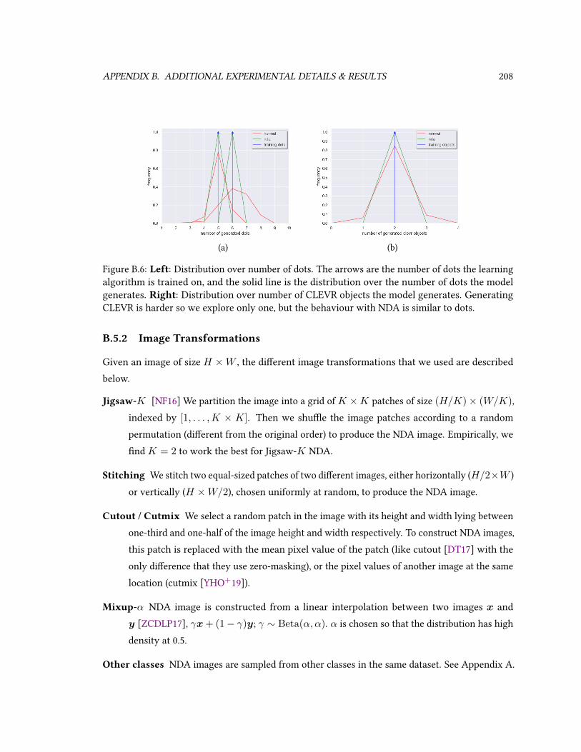
APPENDIX B. ADDITIONAL EXPERIMENTAL DETAILS & RESULTS 208
(a) (b)
Figure B.6: Left: Distribution over number of dots. The arrows are the number of dots the learningalgorithm is trained on, and the solid line is the distribution over the number of dots the modelgenerates. Right: Distribution over number of CLEVR objects the model generates. GeneratingCLEVR is harder so we explore only one, but the behaviour with NDA is similar to dots.
B.5.2 Image Transformations
Given an image of size H ×W , the dierent image transformations that we used are describedbelow.
Jigsaw-K [NF16] We partition the image into a grid of K ×K patches of size (H/K)× (W/K),indexed by [1, . . . ,K × K]. Then we shue the image patches according to a randompermutation (dierent from the original order) to produce the NDA image. Empirically, wend K = 2 to work the best for Jigsaw-K NDA.
Stitching We stitch two equal-sized patches of two dierent images, either horizontally (H/2×W )or vertically (H ×W/2), chosen uniformly at random, to produce the NDA image.
Cutout / Cutmix We select a random patch in the image with its height and width lying betweenone-third and one-half of the image height and width respectively. To construct NDA images,this patch is replaced with the mean pixel value of the patch (like cutout [DT17] with theonly dierence that they use zero-masking), or the pixel values of another image at the samelocation (cutmix [YHO+19]).
Mixup-α NDA image is constructed from a linear interpolation between two images x andy [ZCDLP17], γx+ (1− γ)y; γ ∼ Beta(α, α). α is chosen so that the distribution has highdensity at 0.5.
Other classes NDA images are sampled from other classes in the same dataset. See Appendix A.
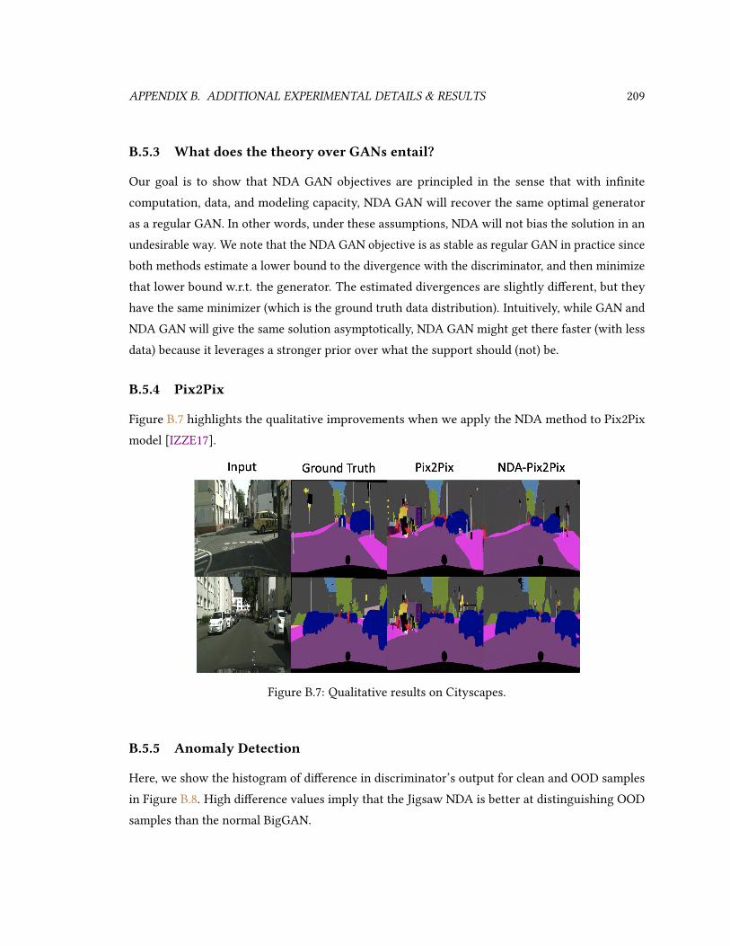
APPENDIX B. ADDITIONAL EXPERIMENTAL DETAILS & RESULTS 209
B.5.3 What does the theory over GANs entail?
Our goal is to show that NDA GAN objectives are principled in the sense that with innitecomputation, data, and modeling capacity, NDA GAN will recover the same optimal generatoras a regular GAN. In other words, under these assumptions, NDA will not bias the solution in anundesirable way. We note that the NDA GAN objective is as stable as regular GAN in practice sinceboth methods estimate a lower bound to the divergence with the discriminator, and then minimizethat lower bound w.r.t. the generator. The estimated divergences are slightly dierent, but theyhave the same minimizer (which is the ground truth data distribution). Intuitively, while GAN andNDA GAN will give the same solution asymptotically, NDA GAN might get there faster (with lessdata) because it leverages a stronger prior over what the support should (not) be.
B.5.4 Pix2Pix
Figure B.7 highlights the qualitative improvements when we apply the NDA method to Pix2Pixmodel [IZZE17].
Figure B.7: Qualitative results on Cityscapes.
B.5.5 Anomaly Detection
Here, we show the histogram of dierence in discriminator’s output for clean and OOD samplesin Figure B.8. High dierence values imply that the Jigsaw NDA is better at distinguishing OODsamples than the normal BigGAN.

APPENDIX B. ADDITIONAL EXPERIMENTAL DETAILS & RESULTS 210
(a) Gaussian Noise (b) Speckle Noise (c) JPEG Compression
Figure B.8: Histogram of D(clean) - D(corrupt) for 3 dierent corruptions.
B.5.6 Eect of hyperparameter on Unconditional Image generation
Here, we show the eect of λ for unconditional image generation on CIFAR-10 dataset.
Table B.4: Eect of λ on the FID score for unconditional image generation on CIFAR-10 usingJigsaw as NDA.
λ 1.0 0.75 0.5 0.25 0.15
FID 18.64 16.61 14.95 12.61 13.01
B.5.7 Unsupervised Learning on Images
0.65 0.45 0.45 0.38 0.57 0.43 0.41 0.36 0.54 0.41 0.50 0.37
Figure B.9: Comparing the cosine distance of the representations learned with Jigsaw NDA andMoco-V2 (shaded blue), and original Moco-V2 (white). With NDA, we project normal and itsjigsaw image representations further away from each other than the one without NDA.

APPENDIX B. ADDITIONAL EXPERIMENTAL DETAILS & RESULTS 211
Dataset Preparation for FID evaluation For dataset preparation, we follow the the followingprocedures: (a) CIFAR-10 contains 60K 32×32 images with 10 labels, out of which 50K are used fortraining and 10K are used for testing, (b) CIFAR-100 contains 60K 32 × 32 images with 100 labels,out of which 50K are used for training and 10K are used for testing, (c) CelebA contains 162,770train images and 19,962 test images (we resize the images to 64×64px), (d) STL-10 contains 100K(unlabeled) train images and 8K (labeled) test images (we resize the images to 32×32px). In ourexperiments the FID is calculated on the test dataset. In particular, we use 10K generated images vs.10K test images for CIFAR-10, 10K vs. 10K for CIFAR-100, 19,962 vs. 19,962 for CelebA, and 8K vs8K for STL-10.
Hyperparameters and Network Architecture
Generative Modeling. We use the same network architecture in BigGAN [BDS18] for ourexperiments. The code used for our experiments is based over the author’s PyTorch code. ForCIFAR-10, CIFAR-100, and CelebA we train for 500 epochs whereas for STL-10 we train for 300epochs. For all the datasets we use the following hyperparameters: batch-size = 64, generatorlearning rate = 2e-4, discriminator learning rate = 2e-4, discriminator update steps per generatorupdate step = 4. The best model was selected on the basis of FID scores on the test set (as explainedabove).
Momentum Contrastive Learning. We use the ocial PyTorch implementation for our ex-periments. For CIFAR-10 and CIFAR-100, we perform unsupervised pre-training for 1000 epochsand supervised training (linear classier) for 100 epochs. For Imagenet-100, we perform unsuper-vised pre-training for 200 epochs and supervised training (linear classier) for 100 epochs. ForCIFAR-10 and CIFAR-100, we use the following hyperparameters during pre-training: batch-size= 256, learning-date = 0.3, temperature = 0.07, feature dimensionality = 2048. For ImageNet-100pre-training we have the following: batch-size = 128, learning-date = 0.015, temperature = 0.2,feature dimensionality = 128. During linear classication we use a batch size of 256 for all thedatasets and learning rate of 10 for CIFAR-10, CIFAR-100, whereas for ImageNet-100 we use learningrate of 30.
Dense Predictive Coding. We use the same network architecture and hyper-parameters inDPC [HXZ19] for our experiments and use the ocial PyTorch implementation. We perform

APPENDIX B. ADDITIONAL EXPERIMENTAL DETAILS & RESULTS 212
self-supervised training on UCF-101 for 200 epochs and supervised training (action classier) for200 epochs on both UCF-101 and HMDB51 datasets.
Code The code to reproduce our experiments is given here.
Implementation Details For our experiment over GAN, we augment the batch of real sampleswith a negative augmentation of the same batch, and we treat the augmented images as fake imagesfor the discriminator. Similarly, for the contrastive learning experiments, we consider negativeaugmentation of the query image batch as negatives for that batch.
For all our experiments we used existing open-source models. For experiments over GAN, weuse the open-source implementations of BigGAN and Pix2Pix models, and for contrastive learning,we use the open-source implementation of the MoCo-v2 model and Dense Predictive Coding. Hence,we did not explain in detail each of the models. Implementing NDA is quite simple as we only needto generate NDA samples from the images in a mini-batch which only takes several lines of code.
Ablation study on negative samples We perform the experiments over MoCo-v2 which main-tains a queue of negative samples. The number of negatives is around 65,536. With our approach,we use the augmented versions of images in the same batch as negative. We transform both the keyand query images to create NDA samples. Thus, the number of negatives for our approach is 65,536+ 2 (one NDA sample created using query image and other using key image), only 0.00003051664times more than the original number of negatives samples in MoCo-v2. Thus our experiments arecomparable to the baseline MoCo-v2. In terms of computation, we need an additional forward passin each batch to get the representations of the NDA samples. The normal MoCo-v2 requires 1.09secs for entire forward computation, which includes forward pass through the network, momentumupdate of the key encoder and dot product between the positive and negative samples. With NDA,1 forward computation requires 1.36 secs.
What happens when negative data augmentations are noisy? Regarding the performanceof negative data augmentation, we perform 2 dierent experiments:
a) When the noise is low - When using jigsaw as our NDA strategy with a 2 x 2 grid, one outof the 24 permutations will be the original image. We nd that when this special permutation isnot removed, or there is 4% “noise”, the FID score is 12.61, but when it is removed the FID scoreis 12.59. So, we nd that when the noise is low, the performance of our approach is not greatlyaected and is robust in such scenarios.

APPENDIX B. ADDITIONAL EXPERIMENTAL DETAILS & RESULTS 213
b) When the noise is large - We use random vertical ipping as our NDA strategy, where with50% probability the image is vertically ipped during NDA. In this case, the “noise” is large, as 50%of the time, the negative sample is actually the original image. We contrast this with the “noise-free”NDA strategy where the NDA image is always vertically ipped. We nd that for the randomvertical ipping NDA, the FID score of BigGAN is 15.84, whereas, with vertical ipping NDA, theFID score of BigGAN is 14.74. So performance degrades with larger amounts of noise.
B.6 Chapter 7
B.6.1 Additional Details for D2C
Contrastive representation learning
In contrastive representation learning, the goal is to distinguish a positive pair (y,w) ∼ p(x,y)
from (m− 1) negative pairs (y,w) ∼ p(x)p(y). In our context, the positive pairs are represen-tations from the same image, and negative pairs are representations from dierent images; theseimages are pre-processed with strong data augmentations [CKNH20] to encourage rich representa-tions. With two random, independent data augmentation procedures dened as aug1 and aug2, wedene p(x,y) and p(x)p(y) via the following sampling procedure:
(y,w) ∼ p(x,y) : y ∼ qφ(z(1)|aug1(x)),w ∼ qφ(z(1)|aug2(x)),x ∼ pdata(x),
(y,w) ∼ p(x)p(y) : y ∼ qφ(z(1)|aug1(x1)),w ∼ qφ(z(1)|aug2(x2)),x1,x2 ∼ pdata(x).
For a batch ofn positive pairs (yi,wi)ni=1, the contrastive predictive coding (CPC, [vdOLV18])objective is dened as:
LCPC(g; qφ) := E
[1
n
n∑i=1
logm · g(xi,yi)
g(xi,yi) +∑m−1
j=1 g(xi,yi,j)
](B.12)
for some positive critic function g : Y × Z → R+, where the expectation is taken over n positivepairs (xi,yi) ∼ p(x,y) and n(m−1) negative pairs (xi,yi,j) ∼ p(x)p(y). Another interpretationto CPC is that it performs m-way classication where the ground truth label is assigned to thepositive pair. The representation learner qφ then aims to maximize the CPC objective, or to minimize

APPENDIX B. ADDITIONAL EXPERIMENTAL DETAILS & RESULTS 214
the following objective:
−LC(qφ) := ming−LCPC(g; qφ), (B.13)
Dierent specic implementations, such as MoCo [HFW+19, CFGH20, CXH21] and SimCLR [CKNH20]can all be treated as specic implementations of this objective function. In this paper, we con-sidered using MoCo-v2 [CKNH20] as our implementation for LC objective; in principle, otherimplementations to CPC can also be integrated into D2C as well.
Training D2C
In Algorithm 7, we describe a high-level procedure that trains the D2C model; we note that thisprocedure does not have any adversarial components. On the high-level, this is the integration ofthree objectives: the reconstruction objective via the autoencoder, the diusion objective over thelatent space, and the contrastive objective over the latent space. In principle, the [reconstruction],[constrastive], and [diusion] components can be optimized jointly or separately; we observethat normalizing the latent z(1) with a global mean and standard deviation before applying thediusion objective helps learning the diusion model with a xed α series.

APPENDIX B. ADDITIONAL EXPERIMENTAL DETAILS & RESULTS 215
Algorithm 7 Training D2CInput: Data distribution pdata.while training do
[Draw samples with data augmentation]
Draw m samples x0:m−1 ∼ pdata(x).Draw (m+ 1) data augmentations aug0, . . . augm−1 and aug0.for i← 0 to m− 1 do
Draw z(1)i ∼ qφ(z(1)|augi(x)).
end forDraw z
(1)0 ∼ qφ(z(1)|aug0(x)).
[Reconstruction]
Reconstruct x0 ∼ pθ(x|z(1)0 )
Minimize Lrecon = − log pθ(x|z(1)0 ) over θ and φ with gradient descent.
[Contrastive]
Dene a classication task: assign label 1 to (z(1)0 , z
(1)0 ) and label 0 to (z
(1)0 , z
(1)i ) for i 6= 0.
Dene LCPC(g; qφ) as the loss to minimize for the above task, with g as the classier.Dene g as a minimizer to the classier objective LCPC(g; qφ).Minimize LCPC(g; qφ) over φ with gradient descent.
[Diusion]
Sample ε ∼ N (0, I), t ∼ Uniform(1, . . . , T ).Dene z(αt)
0 =√αtz
(0)0 +
√1− αtε.
Minimize ‖ε− εθ(z(αt)0 ;αt)‖22 over θ with gradient descent.
end while
B.6.2 Experimental details
Architecture details and hyperparameters used for training
We modify the NVAE [VK20] architecture by removing the “Combiner Cells” in both encoder anddecoder. For the diusion model, we use the same architecture with dierent number of channel mul-tiplications, as used in [HJA20, SME20]. For Contrastive learning, we use the MoCo-v2 [CFGH20]algorithm with augmentations such as RandomResizedCrop, ColorJitter, RandomGrayscale, Ran-
domHorizontalFlip.

APPENDIX B. ADDITIONAL EXPERIMENTAL DETAILS & RESULTS 216
Table B.5: Hyperparameters across dierent datasets
Hyperparameter CIFAR-1032x32
CIFAR-10032x32
CelebA-6464x64
fMoW64x64
CelebA-HQ-256256x256
FFHQ-256256x256
# of epochs 1000 1000 300 300 200 100
batch size per GPU 32 32 16 16 3 3
# initial channels in enc, 128 128 64 64 24 24
spatial dims of z 16*16 16*16 32*32 32*32 64*64 64*64
# channel in z 8 8 5 5 8 8
MoCo-v2 queue size 65536 65536 65536 65536 15000 15000
Diusion feature map res. 16,8,4,2 16,8,4,2 32,16,8,4,1 32,16,8,4,1 64,32,16,8,2 64,32,16,8,2
λ−1 17500 17500 17500 17500 17500 17500
learning rate 0.001 0.001 0.001 0.001 0.001 0.001
Optimizer AdamW AdamW AdamW AdamW AdamW AdamW
# GPUs 8 8 4 4 8 8
GPU Type 16 GB V100 16 GB V100 12 GB Titan X 12 GB Titan X 16 GB V100 16 GB V100
Total training time (h) 24 24 120 120 96 96
Additional details about the hyperparameters used are provided in Table B.5.
Additional details for conditional generation
For rψ(c|z(1)) we consider training a linear model over the latent space, which has the advantageof being computationally ecient. For conditional generation on labels, we reject samples if theirclassier return are lower than a certain threshold (we used 0.5 for all our experiments). Forconditional image manipulation, we consider the same step size η for each attribute: η = 10 for redlipstick and η = 15 for blond. We note that these values are not necessarily the optimal ones, as theintensity of the change can grow with a choice of larger η values.
Amazon Mechanical Turk procedure
The mechanical turk evaluation is done for dierent attributes to nd out how evaluators evaluatethe dierent approaches. The evaluators are asked to compare a pair of images, and nd the bestimage, which retains the identity as well as contains the desired attribute. Figure B.10 a) shows theinstructions that was given to the evaluators before starting the test and Figure B.10 b) containsthe UI shown to the evaluators when doing comparison. Each evaluation task contains 10 pairwisecomparisons, and we perform 15 such evaluation tasks for each attribute. The reward per task iskept as 0.25$. Since each task takes around 2.5 mins, so the hourly wage comes to be 6$ per hour.

APPENDIX B. ADDITIONAL EXPERIMENTAL DETAILS & RESULTS 217
Figure B.10: a) Instructions shown to human evaluators for Amazon Mechanical Turk for blondhair before starting the evaluation and b) UI shown to the evaluators when doing comparison.

APPENDIX B. ADDITIONAL EXPERIMENTAL DETAILS & RESULTS 218
Table B.6: CIFAR-10 image generation results.
Method FID
NVAE [VK20] 51.71NCP-VAE [ASKV20] 24.08EBM [DM19] 40.58StyleGAN2 [KLA+20] 3.26DDPM [HJA20] 3.17DDIM [SME20] 4.04D2C 10.15
B.6.3 Additional Results
We list results for unconditional CIFAR-10 image generation for various types of generative modelsin Table B.6. While our results are slightly worse than state-of-the-art diusion models, we notethat our D2C models are trained with relatively fewer resources that some of the baselines; forexample, our D2C models is trained on 8 GPUs for 24 hours, whereas NVAE is trained on 8 GPUsfor 100 hours and DDPM is trained on v3-8 TPUs for 24 hours. We also note that these comparisonsare not necessarily fair in terms of the architecture and compute used to produce the samples.
We list additional image generation results in Figure B.11 (unconditional), Figures B.12, B.13, B.14,and B.15 (conditional on manipulation constraints), and Figures B.16, B.17, B.18, and B.19 (condi-tional on labels)2.
B.7 Chapter 8
B.7.1 Estimating Eective Sample Size
Assume a target distribution p(x), and a Markov chain Monte Carlo (MCMC) sampler that producesa set of N correlated samples xiN1 from some distribution q(xiN1 ) such that q(xi) = p(xi).Suppose we are estimating the mean of p(x) through sampling; we assume that increasing thenumber of samples will reduce the variance of that estimate.
Let V = Varq[∑N
i=1 xi/N ] be the variance of the mean estimate through the MCMC sam-ples. The eective sample size (ESS) of xiN1 , which we denote as M = ESS(xiN1 ), is thenumber of independent samples from p(x) needed in order to achieve the same variance, i.e.
2We will list more results online after publication.

APPENDIX B. ADDITIONAL EXPERIMENTAL DETAILS & RESULTS 219
Figure B.11: Additional image samples for the FFHQ-256 dataset.

APPENDIX B. ADDITIONAL EXPERIMENTAL DETAILS & RESULTS 220
Original D2C StyleGAN2 NVAE DDIM
Figure B.12: Image manipulation results for blond hair.

APPENDIX B. ADDITIONAL EXPERIMENTAL DETAILS & RESULTS 221
Original D2C StyleGAN2 NVAE DDIM
Figure B.13: Image manipulation results for red lipstick.

APPENDIX B. ADDITIONAL EXPERIMENTAL DETAILS & RESULTS 222
Original D2C StyleGAN2 NVAE DDIM
Figure B.14: Image manipulation results for beard.

APPENDIX B. ADDITIONAL EXPERIMENTAL DETAILS & RESULTS 223
Original D2C StyleGAN2 NVAE DDIM
Figure B.15: Image manipulation results for gender.
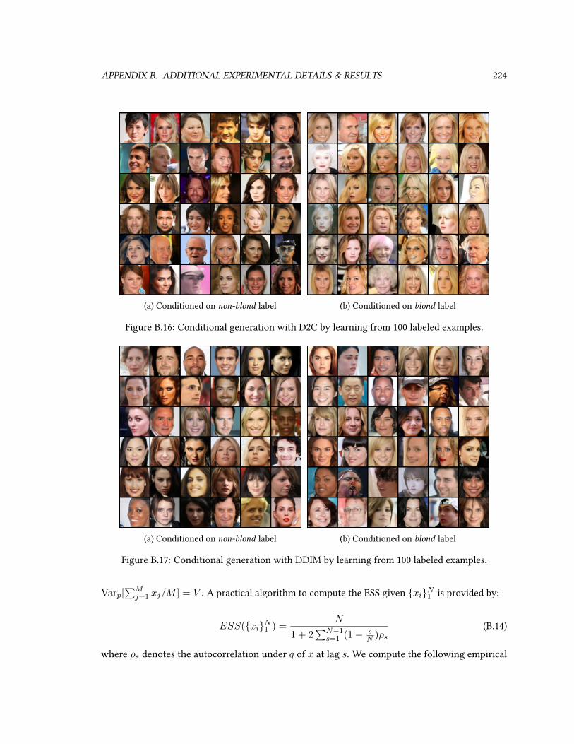
APPENDIX B. ADDITIONAL EXPERIMENTAL DETAILS & RESULTS 224
(a) Conditioned on non-blond label (b) Conditioned on blond label
Figure B.16: Conditional generation with D2C by learning from 100 labeled examples.
(a) Conditioned on non-blond label (b) Conditioned on blond label
Figure B.17: Conditional generation with DDIM by learning from 100 labeled examples.
Varp[∑M
j=1 xj/M ] = V . A practical algorithm to compute the ESS given xiN1 is provided by:
ESS(xiN1 ) =N
1 + 2∑N−1
s=1 (1− sN )ρs
(B.14)
where ρs denotes the autocorrelation under q of x at lag s. We compute the following empirical

APPENDIX B. ADDITIONAL EXPERIMENTAL DETAILS & RESULTS 225
(a) Conditioned on female label (b) Conditioned on male label
Figure B.18: Conditional generation with D2C by learning from 100 labeled examples.
(a) Conditioned on female label (b) Conditioned on male label
Figure B.19: Conditional generation with DDIM by learning from 100 labeled examples.
estimate ρs for ρs:
ρs =1
σ2(N − s)N∑
n=s+1
(xn − µ)(xn−s − µ) (B.15)
where µ and σ are the empirical mean and variance obtained by an independent sampler.

APPENDIX B. ADDITIONAL EXPERIMENTAL DETAILS & RESULTS 226
Due to the noise in large lags s, we adopt the approach of [HG14] where we truncate the sumover the autocorrelations when the autocorrelation goes below 0.05.
B.7.2 Justications for Objective in Equation 9.3
We consider two necessary conditions for pd to be the stationary distribution of the Markov chain,which can be translated into a new algorithm with better optimization properties, described inEquation 9.3.
Proposition 8. Consider a sequence of ergodic Markov chains over state space S . Dene πn as the
stationary distribution for the n-th Markov chain, and πtn as the probability distribution at time step t
for the n-th Markov chain. If the following two conditions hold:
1. ∃b > 0 such that the sequence πbn∞n=1 converges to pd in total variation;
2. ∃ε > 0, ρ < 1 such that ∃M > 0,∀n > M , if ‖πtn − pd‖TV< ε, then ‖πt+1n − pd‖TV<
ρ‖πtn − pd‖TV ;
then the sequence of stationary distributions πn∞n=1 converges to pd in total variation.
Proof. The goal is to prove that ∀δ > 0, ∃K > 0, T > 0, such that ∀n > N, t > T , ‖πtn−pd‖TV< δ.According to the rst assumption, ∃N > 0, such that ∀n > N , ‖πbn − pd‖TV< ε.Therefore, ∀n > K = max(N,M), ∀δ > 0, ∃T = b+ max(0, dlogρ δ− logρ εe) + 1, such that
∀t > T ,
‖πtn − pd‖TV
=‖πbn − pd‖TV
t−1∏i=b
‖πi+1n − pd‖TV‖πin − pd‖TV
< ερt−b < ερT−b < ε · δε
= δ (B.16)
The rst inequality uses the fact that ‖πbn − pd‖TV< ε (from Assumption 1), and ‖πt+1n −
pd‖TV/‖πtn − pd‖TV< ρ (from Assumption 2). The second inequality is true because ρ < 1 byAssumption 2. The third inequality uses the fact that T − b > dlogρ δ − logρ εe (from denition ofT ), so ρT−b < δ/ε. Hence the sequence πn∞n=1 converges to pd in total variation.
Moreover, convergence in total variation distance is equivalent to convergence in Jensen-Shannon (JS) divergence[ACB17], which is what GANs attempt to minimize [GPAM+14]. This

APPENDIX B. ADDITIONAL EXPERIMENTAL DETAILS & RESULTS 227
motivates the use of GANs to achieve the two conditions in Proposition 8. This suggests a newoptimization criterion, where we look for a θ that satises both conditions in Proposition 8, whichtranslates to Equation 9.3.
B.7.3 Details on the Pairwise Discriminator
Similar to the settings in MGAN objective, we consider two chains to obtain samples:
• Starting from a data point x, sample z1 in B steps.
• Starting from some noise z, sample z2 in B steps; and from z2 sample z3 in M steps.
For the “generated” (fake) data, we use two type of pairs (x, z1), and (z2, z3). This is illustratedin Figure B.20. We assume equal weights between the two types of pairs.
no gradient gradient
x
z
z1|x
z2|z z2 z3|z2
pair
Figure B.20: Illustration of the generative process for the pairwise discriminator. We block thegradient for z2 to further parallelize the process and improve training speed.

APPENDIX B. ADDITIONAL EXPERIMENTAL DETAILS & RESULTS 228
B.7.4 Additional Experimental Details
Architectures for Generative Model for Images
Code is available at https://github.com/ermongroup/markov-chain-gan.Let ‘fc n, (activation)’ denote a fully connected layer with n neurons. Let ‘conv2d n, k, s,
(activation)’ denote a convolutional layer with n lters of size k and stride s. Let ‘deconv2d n, k, s,(activation)’ denote a transposed convolutional layer with n lters of size k and stride s.
We use the following model to generate Figure 9.1 (MNIST).
encoder decoder discriminator
fc 600, lrelu fc 600, lrelu conv2d 64, 4× 4, 2× 2, relufc 100, linear fc 784, sigmoid conv2d 128, 4× 4, 2× 2, lrelu
fc 600, lrelufc 1, linear
We use the following model to generate Figure 9.3 (CelebA, top)
encoder decoder discriminator
conv2d 64, 4× 4, 2× 2, lrelu fc 16× 16× 64, lrelu conv2d 64, 4× 4, 2× 2, relufc 200, linear deconv2d 3, 4× 4, 2× 2, tanh conv2d 128, 4× 4, 2× 2, lrelu
conv2d 256, 4× 4, 2× 2, lrelufc 1, linear
For the bottom gure in Figure 9.3, we add a residual connection such that the input to thesecond layer of the decoder is the sum of the outputs from the rst layers of the decoder andencoder (both have shape 16× 16× 64); we add a highway connection from input image to theoutput of the decoder:
x = αx+ (1− α)x
where x is the output of the function, x is the output of the decoder, andα is an additional transposedconvolutional output layer with sigmoid activation that has the same dimension as x.
We use the following model to generate Figure 9.5 (CelebA, pairwise):
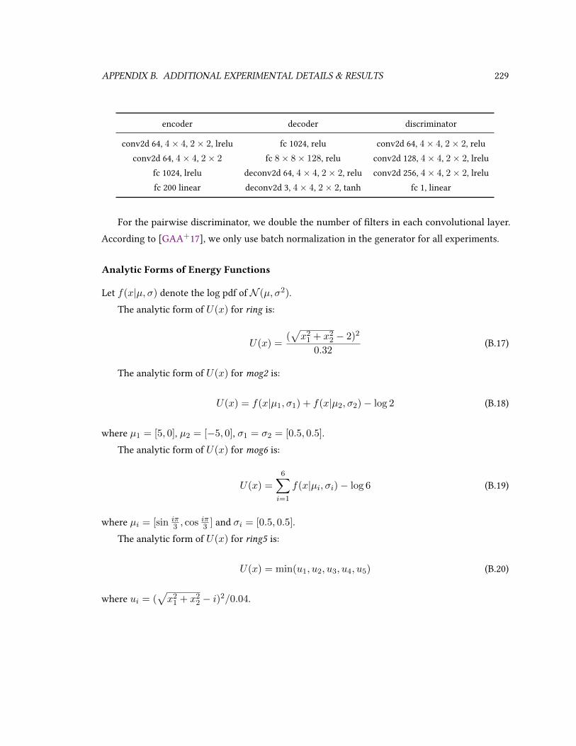
APPENDIX B. ADDITIONAL EXPERIMENTAL DETAILS & RESULTS 229
encoder decoder discriminator
conv2d 64, 4× 4, 2× 2, lrelu fc 1024, relu conv2d 64, 4× 4, 2× 2, reluconv2d 64, 4× 4, 2× 2 fc 8× 8× 128, relu conv2d 128, 4× 4, 2× 2, lrelu
fc 1024, lrelu deconv2d 64, 4× 4, 2× 2, relu conv2d 256, 4× 4, 2× 2, lrelufc 200 linear deconv2d 3, 4× 4, 2× 2, tanh fc 1, linear
For the pairwise discriminator, we double the number of lters in each convolutional layer.According to [GAA+17], we only use batch normalization in the generator for all experiments.
Analytic Forms of Energy Functions
Let f(x|µ, σ) denote the log pdf of N (µ, σ2).The analytic form of U(x) for ring is:
U(x) =(√x2
1 + x22 − 2)2
0.32(B.17)
The analytic form of U(x) for mog2 is:
U(x) = f(x|µ1, σ1) + f(x|µ2, σ2)− log 2 (B.18)
where µ1 = [5, 0], µ2 = [−5, 0], σ1 = σ2 = [0.5, 0.5].The analytic form of U(x) for mog6 is:
U(x) =6∑i=1
f(x|µi, σi)− log 6 (B.19)
where µi = [sin iπ3 , cos iπ3 ] and σi = [0.5, 0.5].
The analytic form of U(x) for ring5 is:
U(x) = min(u1, u2, u3, u4, u5) (B.20)
where ui = (√x2
1 + x22 − i)2/0.04.

APPENDIX B. ADDITIONAL EXPERIMENTAL DETAILS & RESULTS 230
Benchmarking Running Time
Since the runtime results depends on the type of machine, language, and low-level optimizations,we try to make a fair comparison between HMC and A-NICE-MC on TensorFlow [AAB+16].
Our code is written and executed in TensorFlow 1.0. Due to the optimization of the computationgraphs in TensorFlow, the wall-clock time does not seem to be exactly linear in some cases, evenwhen we force the program to use only 1 thread on the CPU. The wall-clock time is aected by 2aspects, batch size and number of steps. We nd that the wall-clock time is relatively linear withrespect to the number of steps, and not exactly linear with respect to the batch size.
Given a xed number of steps, the wall-clock time is constant when the batch size is lowerthan a threshold, and then increases approximately linearly. To perform speed benchmarking onthe methods, we select the batch size to be the value around the threshold, in order to preventsignicant under-estimates of the eciency.
We found that the graph is much more optimized if the batch size is determined before execution.Therefore, we perform all the benchmarks on the optimized graph where we specify a batch sizeprior to running the graph. For the energy functions, we use a batch size of 2000; for Bayesianlogistic regression we use a batch size of 64.
Hyperparameters for the Energy Function Experiments
For all the experiments, we use same hyperparameters for both A-NICE-MC and HMC. We samplex0 ∼ N (0, I) and run the chain for 1000 burn-in steps and evaluate the samples from the next1000 steps. For HMC we use 40 leapfrog steps and a step size of 0.1. For A-NICE-MC we considerfθ(x, v) with three coupling layers, which updates v, x and v respectively. The motivation behindthis particular architecture is to ensure that both x and v could aect the updates to x′ and v′.In each coupling layer, we select the function m(·) to be a one-layer NN with 400 neurons. Thediscriminator is a three layer MLP with 400 neurons each. Similar to the settings in Section 9.3.1,we use the gradient penalty method in [GAA+17] to train our model. For bootstrapping, we rstcollect samples by running the NICE proposal over the untrained fθ , and for every 500 iterationswe replace half of the samples with samples from the latest trained model. All the models aretrained with AdaM [KB14] for 20000 iterations with B = 4, M = 2, batch size of 32 and learningrate of 10−4.

APPENDIX B. ADDITIONAL EXPERIMENTAL DETAILS & RESULTS 231
Hyperparameters for the Bayesian Logistic Regression Experiments
For HMC we tuned the step size parameter to achieve the best ESS possible on each dataset, whichis 0.005 for german, 0.01 for heart and 0.0115 for australian (HMC performance on australian isextremely sensitive to the step size). For A-NICE-MC we consider f(x, v) with three couplinglayers, which updates v, x and v respectively; we set v to have 50 dimensions in all the experiments.m(·) is a one-layer NN with 400 neurons for the top and bottom coupling layer, and a two-layerNN with 400 neurons each for the middle layer. The discriminator is a three layer MLP with 800neurons each. We use the same training and bootstrapping strategy as in Appendix B.7.4. All themodels are trained with AdaM for 20000 iterations with B = 16, M = 2, batch size of 32 andlearning rate of 5× 10⁻⁴.
Architecture Details
The following gure illustrates the architecture details of fθ(x, v) for A-NICE-MC experiments.We do not use batch normalization (or other normalization techniques), since it slows the executionof the network and does not provide much ESS improvement.
fc 400, relu
fc 400, relu
fc 400, relu
sum
sum
sum
v ∼ N (0, I)x
v′x′
identity
identity
identity
(a) NICE architecture for energy functions.
fc 400, relu
fc 400, relu
fc 400, relu
sum
sum
sum
v ∼ N (0, I)x
v′x′
identity
identity
identity
fc 400, relu
(b) NICE architecture for Bayesian logistic regres-sion.

APPENDIX B. ADDITIONAL EXPERIMENTAL DETAILS & RESULTS 232
B.8 Chapter 9
B.8.1 MAGAIL Algorithm
We include the MAGAIL algorithm as follows:
Algorithm 8 Multi-Agent GAIL (MAGAIL)Input: Initial parameters of policies, discriminators and value (baseline) estimators θ0, ω0, φ0; experttrajectories D = (sj , aj)Mj=0; batch size B; Markov game as a black box (N,S,A, η, T, r,o, γ).Output: Learned policies πθ and reward functions Dω .for u = 0, 1, 2, . . . do
Obtain trajectories of size B from π by the process: s0 ∼ η(s), at ∼ πθu(at|st), st+1 ∼ P (st|at).Sample state-action pairs from D with batch size B.Denote state-action pairs from π and D as χ and χE .for i = 1, . . . , n do
Update ωi to increase the objective
Eχ[logDωi(s, ai)] + EχE
[log(1−Dωi(s, ai))]
end forfor i = 1, . . . , n do
Compute value estimate V ? and advantage estimate Ai for (s, a) ∈ χ.Update φi to decrease the objective
Eχ[(Vφ(s, a−i)− V ?(s, a−i))2]
Update θi by policy gradient with small step sizes:
Eχ[∇θiπθi(ai|oi)Ai(s, a)]
end forend for
B.8.2 Experiment Details
Hyperparameters
For the particle environment, we use two layer MLPs with 128 cells in each layer, for the policygenerator network, value network and the discriminator. We use a batch size of 1000. The policy istrained using K-FAC optimizer [MG15] with learning rate of 0.1. All other parameters for K-FAC

APPENDIX B. ADDITIONAL EXPERIMENTAL DETAILS & RESULTS 233
Table B.7: Performance in cooperative navigation.
# Expert Episodes 100 200 300 400Expert -13.50 ± 6.3
Random -128.13 ± 32.1Behavior Cloning -56.82 ± 18.9 -43.10 ± 16.0 -35.66 ± 15.2 -25.83 ± 12.7
Centralized -46.66 ± 20.8 -23.10 ± 12.4 -21.53 ± 12.9 -15.30 ± 7.0Decentralized -50.00 ± 18.6 -25.61 ± 12.3 -24.10 ± 13.3 -15.55 ± 6.5
GAIL -55.01 ± 17.7 -39.21 ± 16.5 -29.89 ± 13.5 -18.76 ± 12.1
Table B.8: Performance in cooperative communication.
# Expert Episodes 100 200 300 400Expert -6.22 ± 4.5
Random -62.49 ± 28.7Behavior Cloning -21.25 ± 10.6 -13.25 ± 7.4 -11.37 ± 5.9 -10.00 ± 5.36
Centralized -15.65 ± 10.0 -7.11 ± 4.8 -7.11 ± 4.8 -7.09 ± 4.8Decentralized -18.68 ± 10.4 -8.06 ± 5.3 -8.16 ± 5.5 -7.34 ± 4.9
GAIL -20.28 ± 10.1 -11.06 ± 7.8 -10.51 ± 6.6 -9.44 ± 5.7
optimizer are the same in [WMG+17].For the cooperative control task, we use two layer MLPs with 64 cells in each layer for all the
networks. We use a batch size of 2048, and learning rate of 0.03. We obtain expert trajectories bytraining the expert with MACK and sampling demonstrations from the same environment. Hence,the expert’s demonstrations are imperfect (or even awed) in the environment that we test on.
Detailed Results
We use the particle environment introduced in [LWT+17] and the multi-agent control environ-ment [KGE17] for experiments. We list the exact performance in Tables B.7, B.8 for cooperativetasks, and Table B.9 and competitive tasks. The means and standard deviations are computed over100 episodes. The policies in the cooperative tasks are trained with varying number of expertdemonstrations. The policies in the competitive tasks are trained with on a dataset with 100 experttrajectories.
The environment for each episode is drastically dierent (e.g. location of landmarks arerandomly sampled), which leads to the seemingly high standrad deviation across episodes.

APPENDIX B. ADDITIONAL EXPERIMENTAL DETAILS & RESULTS 234
Table B.9: Performance in competitive tasks.
Task Agent Policy Adversary Policy Agent Reward
Predator-Prey
Behavior Cloning
Behavior Cloning -93.20 ± 63.7GAIL -93.71 ± 64.2
Centralized -93.75 ± 61.9Decentralized -95.22 ± 49.7
Zero-Sum -95.48 ± 50.4GAIL
Behavior Cloning
-90.55 ± 63.7Centralized -91.36 ± 58.7
Decentralized -85.00 ± 42.3Zero-Sum -89.4 ± 48.2
Keep-Away
Behavior Cloning
Behavior Cloning 24.22 ± 21.1GAIL 24.04 ± 18.2
Centralized 23.28 ± 20.6Decentralized 23.56 ± 19.9
Zero-Sum 23.19 ± 19.9GAIL
Behavior Cloning
26.22 ± 19.1Centralized 26.61 ± 20.0
Decentralized 28.73 ± 18.3Zero-Sum 27.80 ± 19.2
1M 2M 4M 6M 8M 10M
0.5
0.0
0.5
1.0
Cooperative Communication
1M 2M 4M 6M 8M 10M
0.50
0.25
0.00
0.25
0.50
0.75
1.00Cooperative Navigation
Powered by TCPDF (www.tcpdf.org)
Cooperative Decentralized BC Expert
Number of Timesteps
Episo
de R
ewar
ds
Number of Timesteps
Figure B.22: Sample complexity of multi-agent GAIL methods under cooperative tasks. Performanceof experts is normalized to one, and performance of behavior cloning is normalized to zero. Thestandard deviation is computed with respect to episodes, and is noisy due to randomness in theenvironment.

APPENDIX B. ADDITIONAL EXPERIMENTAL DETAILS & RESULTS 235
Video Demonstrations
We show certain trajectories generated by our methods. The vidoes are here: videos3.For the particle case:
Navigation-BC-Agents.gif Agents trained by behavior cloning in the navigation task.
Navigation-GAIL-Agents.gif Agents trained by proposed framework in the navigation task.
Predator-Prey-BC-Agent-BC-Adversary.gif Agent (green) trained by behavior cloning playagainst adversaries (red) trained by behavior cloning.
Predator-Prey-GAIL-Agent-BC-Adversary.gif Agent (green) trained by proposed frameworkplay against adversaries (red) trained by behavior cloning.
For the cooperative control case:
Multi-Walker-Expert.mp4 Expert demonstrations in the “easy” environment.
Multi-Walker-GAIL.mp4 Centralized GAIL trained on the “hard” environment.
Multi-Walker-BC.mp4 BC trained on the “hard” environment.
Interestingly, the failure modes for the agents in “hard” environment is mostly having the plankfall o or bounce o, since by decreasing the weight of the plank will decrease its friction force andincrease its acceleration.
3https://drive.google.com/open?id=1Oz4ezMaKiIsPUKtCEOb6YoHJ9jLk6zbj

Appendix C
Code and Data
The following links provide open-source implementations and custom datasets (if applicable) forthe various chapters presented in this dissertation.
• Chapter 2https://github.com/ermongroup/smile-mi-estimator
• Chapter 3https://github.com/jiamings/ml-cpc
• Chapter 4https://github.com/jiamings/lag-fairness
• Chapter 5https://github.com/ermongroup/f-wgan
• Chapter 6https://github.com/ermongroup/NDA
• Chapter 7https://github.com/jiamings/d2c
• Chapter 8https://github.com/ermongroup/a-nice-mc
• Chapter 9https://github.com/ermongroup/multiagent-gail
https://github.com/ermongroup/MA-AIRL
236

Bibliography
[AAB+16] Martín Abadi, Ashish Agarwal, Paul Barham, Eugene Brevdo, Zhifeng Chen, CraigCitro, Greg S Corrado, Andy Davis, Jerey Dean, Matthieu Devin, et al. Tensorow:Large-scale machine learning on heterogeneous distributed systems. arXiv preprintarXiv:1603.04467, 2016.
[AABS19] Jyoti Aneja, Harsh Agrawal, Dhruv Batra, and Alexander Schwing. Sequential latentspaces for modeling the intention during diverse image captioning. In Proceedings
of the IEEE/CVF International Conference on Computer Vision, pages 4261–4270, 2019.
[AAH19] Muhammad Asim, Ali Ahmed, and Paul Hand. Invertible generative models forinverse problems: mitigating representation error and dataset bias. arXiv preprintarXiv:1905.11672, May 2019.
[AC16] Dario Amodei and Jack Clark. Faulty reward functions in the wild, 2016.
[ACB17] Martin Arjovsky, Soumith Chintala, and Léon Bottou. Wasserstein GAN. arXiv
preprint arXiv:1701.07875, January 2017.
[AFDM16] Alexander A Alemi, Ian Fischer, Joshua V Dillon, and Kevin Murphy. Deep variationalinformation bottleneck. arXiv preprint arXiv:1612.00410, December 2016.
[AHD+19] Sungsoo Ahn, Shell Xu Hu, Andreas Damianou, Neil D Lawrence, and Zhenwen Dai.Variational information distillation for knowledge transfer. In Proceedings of the
IEEE Conference on Computer Vision and Pattern Recognition, pages 9163–9171, 2019.
[Ama98] Shun-Ichi Amari. Natural gradient works eciently in learning. Neural computation,10(2):251–276, February 1998.
237

BIBLIOGRAPHY 238
[AN04] Pieter Abbeel and Andrew Y Ng. Apprenticeship learning via inverse reinforcementlearning. In Proceedings of the twenty-rst international conference on Machine
learning, page 1. ACM, 2004.
[AN07] Arthur Asuncion and David Newman. UCI machine learning repository, 2007.
[AOD+18] Samaneh Azadi, Catherine Olsson, Trevor Darrell, Ian Goodfellow, and AugustusOdena. Discriminator rejection sampling. arXiv preprint arXiv:1810.06758, October2018.
[AOS+16] Dario Amodei, Chris Olah, Jacob Steinhardt, Paul Christiano, John Schulman, andDan Mané. Concrete problems in AI safety. arXiv preprint arXiv:1606.06565, June2016.
[APF+17] Alexander A Alemi, Ben Poole, Ian Fischer, Joshua V Dillon, Rif A Saurous, andKevin Murphy. Fixing a broken ELBO. arXiv preprint arXiv:1711.00464, November2017.
[ARV19] Yuki M Asano, Christian Rupprecht, and Andrea Vedaldi. A critical analysisof self-supervision, or what we can learn from a single image. arXiv preprint
arXiv:1904.13132, 2019.
[AS66] Syed Mumtaz Ali and Samuel D Silvey. A general class of coecients of divergenceof one distribution from another. Journal of the Royal Statistical Society: Series B(Methodological), 28(1):131–142, 1966.
[ASE17] Antreas Antoniou, Amos Storkey, and Harrison Edwards. Data augmentationgenerative adversarial networks. arXiv preprint arXiv:1711.04340, November 2017.
[ASKV20] Jyoti Aneja, Alexander Schwing, Jan Kautz, and Arash Vahdat. NCP-VAE: Variationalautoencoders with noise contrastive priors. arXiv preprint arXiv:2010.02917, October2020.
[Aum74] Robert J Aumann. Subjectivity and correlation in randomized strategies. Journal ofmathematical Economics, 1(1):67–96, 1974.
[Aum87] Robert J Aumann. Correlated equilibrium as an expression of bayesian rationality.Econometrica: Journal of the Econometric Society, pages 1–18, 1987.

BIBLIOGRAPHY 239
[BA03] David Barber and Felix V Agakov. The IM algorithm: a variational approach toinformation maximization. In Advances in neural information processing systems,page None. researchgate.net, 2003.
[Bag15] J Andrew Bagnell. An invitation to imitation. Technical report, CARNEGIE-MELLONUNIV PITTSBURGH PA ROBOTICS INST, 2015.
[Bar89] Horace B Barlow. Unsupervised learning. Neural computation, 1(3):295–311, 1989.
[BB14] Michael Bloem and Nicholas Bambos. Innite time horizon maximum causal entropyinverse reinforcement learning. In Decision and Control (CDC), 2014 IEEE 53rd Annual
Conference on, pages 4911–4916. IEEE, 2014.
[BBR+18] Mohamed Ishmael Belghazi, Aristide Baratin, Sai Rajeswar, Sherjil Ozair, YoshuaBengio, Aaron Courville, and R Devon Hjelm. MINE: Mutual information neuralestimation. arXiv preprint arXiv:1801.04062, January 2018.
[BD14] Kenneth Bogert and Prashant Doshi. Multi-robot inverse reinforcement learningunder occlusion with interactions. In Proceedings of the 2014 international confer-
ence on Autonomous agents and multi-agent systems, pages 173–180. InternationalFoundation for Autonomous Agents and Multiagent Systems, 2014.
[BDS18] Andrew Brock, Je Donahue, and Karen Simonyan. Large scale GAN training forhigh delity natural image synthesis. arXiv preprint arXiv:1809.11096, September2018.
[BDX04] Stephen Boyd, Persi Diaconis, and Lin Xiao. Fastest mixing markov chain on a graph.SIAM review, 46(4):667–689, 2004.
[BG98] Stephen P Brooks and Andrew Gelman. General methods for monitoring conver-gence of iterative simulations. Journal of computational and graphical statistics,7(4):434–455, 1998.
[BGR+06] Karsten M Borgwardt, Arthur Gretton, Malte J Rasch, Hans-Peter Kriegel, BernhardSchölkopf, and Alex J Smola. Integrating structured biological data by kernelmaximum mean discrepancy. Bioinformatics, 22(14):e49–57, July 2006.
[BHV17] Floria Bordes, Sina Honari, and Pascal Vincent. Learning to generate samples fromnoise through infusion training. ICLR, 2017.

BIBLIOGRAPHY 240
[BKB18] Shane T Barratt, Mykel J Kochenderfer, and Stephen P Boyd. Learning probabilistictrajectory models of aircraft in terminal airspace from position data. IEEE Transac-
tions on Intelligent Transportation Systems, 2018.
[BL18] Jonathon Byrd and Zachary C Lipton. What is the eect of importance weightingin deep learning? arXiv preprint arXiv:1812.03372, 2018.
[BLC18] Avishek Joey Bose, Huan Ling, and Yanshuai Cao. Adversarial contrastive estimation.In Proceedings of the 56th Annual Meeting of the Association for Computational
Linguistics (Volume 1: Long Papers), pages 1021–1032, 2018.
[BLCW09] Yoshua Bengio, Jérôme Louradour, Ronan Collobert, and Jason Weston. Curriculumlearning. In Proceedings of the 26th annual international conference on machine
learning, pages 41–48, 2009.
[BLRW16] Andrew Brock, Theodore Lim, James M Ritchie, and Nick Weston. Neural photoediting with introspective adversarial networks. arXiv preprint arXiv:1609.07093,2016.
[BMR+20] Tom B Brown, Benjamin Mann, Nick Ryder, Melanie Subbiah, Jared Kaplan, Pra-fulla Dhariwal, Arvind Neelakantan, Pranav Shyam, Girish Sastry, Amanda Askell,Sandhini Agarwal, Ariel Herbert-Voss, Gretchen Krueger, Tom Henighan, RewonChild, Aditya Ramesh, Daniel M Ziegler, Jerey Wu, Clemens Winter, ChristopherHesse, Mark Chen, Eric Sigler, Mateusz Litwin, Scott Gray, Benjamin Chess, JackClark, Christopher Berner, Sam McCandlish, Alec Radford, Ilya Sutskever, and DarioAmodei. Language models are Few-Shot learners. arXiv preprint arXiv:2005.14165,May 2020.
[BS95] Anthony J Bell and Terrence J Sejnowski. An information-maximization approachto blind separation and blind deconvolution. Neural computation, 7(6):1129–1159,1995.
[BTLAY14] Yoshua Bengio, Eric Thibodeau-Laufer, Guillaume Alain, and Jason Yosinski. Deepgenerative stochastic networks trainable by backprop. 2014.
[BV18] Sergey Bartunov and Dmitry Vetrov. Few-shot generative modelling with generativematching networks. In Amos Storkey and Fernando Perez-Cruz, editors, Proceedings

BIBLIOGRAPHY 241
of the Twenty-First International Conference on Articial Intelligence and Statistics,volume 84 of Proceedings of Machine Learning Research, pages 670–678. PMLR, 2018.
[BZW+19] David Bau, Jun-Yan Zhu, Jonas Wul, William Peebles, Hendrik Strobelt, Bolei Zhou,and Antonio Torralba. Seeing what a gan cannot generate. In Proceedings of the
IEEE/CVF International Conference on Computer Vision, pages 4502–4511, 2019.
[CD19] Louis Clouâtre and Marc Demers. Figr: Few-shot image generation with reptile.arXiv preprint arXiv:1901.02199, 2019.
[CDH+16] Xi Chen, Yan Duan, Rein Houthooft, John Schulman, Ilya Sutskever, and PieterAbbeel. InfoGAN: Interpretable representation learning by information maximizinggenerative adversarial nets. arXiv preprint arXiv:1606.03657, pages 2172–2180, June2016.
[CFGH20] Xinlei Chen, Haoqi Fan, Ross Girshick, and Kaiming He. Improved baselines withmomentum contrastive learning. arXiv preprint arXiv:2003.04297, March 2020.
[CFWM18] Gordon Christie, Neil Fendley, James Wilson, and Ryan Mukherjee. Functional mapof the world. In Proceedings of the IEEE Conference on Computer Vision and Pattern
Recognition, pages 6172–6180, 2018.
[CH20] Xinlei Chen and Kaiming He. Exploring simple siamese representation learning.arXiv preprint arXiv:2011.10566, November 2020.
[Chi20] Rewon Child. Very deep vaes generalize autoregressive models and can outperformthem on images. arXiv preprint arXiv:2011.10650, 2020.
[Cho17] Alexandra Chouldechova. Fair prediction with disparate impact: A study of bias inrecidivism prediction instruments. Big data, 5(2):153–163, June 2017.
[CJL+19] Yin Cui, Menglin Jia, Tsung-Yi Lin, Yang Song, and Serge Belongie. Class-Balancedloss based on eective number of samples. arXiv preprint arXiv:1901.05555, January2019.
[CK17] Qifeng Chen and Vladlen Koltun. Photographic image synthesis with cascadedrenement networks. In ICCV, 2017.

BIBLIOGRAPHY 242
[CKNH20] Ting Chen, Simon Kornblith, Mohammad Norouzi, and Georey Hinton. A sim-ple framework for contrastive learning of visual representations. arXiv preprint
arXiv:2002.05709, February 2020.
[CKP09] Toon Calders, Faisal Kamiran, and Mykola Pechenizkiy. Building classiers withindependency constraints. In 2009 IEEE International Conference on Data Mining
Workshops, pages 13–18. IEEE, 2009.
[CKS+16] Xi Chen, Diederik P Kingma, Tim Salimans, Yan Duan, Prafulla Dhariwal, JohnSchulman, Ilya Sutskever, and Pieter Abbeel. Variational lossy autoencoder. arXivpreprint arXiv:1611.02731, November 2016.
[CMK+14] M. Cimpoi, S. Maji, I. Kokkinos, S. Mohamed, , and A. Vedaldi. Describing textures inthe wild. In Proceedings of the IEEE Conf. on Computer Vision and Pattern Recognition
(CVPR), 2014.
[COR+16] Marius Cordts, Mohamed Omran, Sebastian Ramos, Timo Rehfeld, Markus Enzweiler,Rodrigo Benenson, Uwe Franke, Stefan Roth, and Bernt Schiele. The cityscapesdataset for semantic urban scene understanding. In Proceedings of the IEEE conference
on computer vision and pattern recognition, pages 3213–3223, 2016.
[CRBD18] Ricky T Q Chen, Yulia Rubanova, Jesse Bettencourt, and David Duvenaud. Neuralordinary dierential equations. arXiv preprint arXiv:1806.07366, June 2018.
[CRT06] Emmanuel J Candes, Justin K Romberg, and Terence Tao. Stable signal recovery fromincomplete and inaccurate measurements. Communications on Pure and Applied
Mathematics: A Journal Issued by the Courant Institute of Mathematical Sciences,59(8):1207–1223, 2006.
[Csi64] Imre Csiszár. Eine informationstheoretische ungleichung und ihre anwendung aufbeweis der ergodizitaet von markoschen ketten. Magyer Tud. Akad. Mat. Kutato
Int. Koezl., 8:85–108, 1964.
[CWG+19] Kaidi Cao, Colin Wei, Adrien Gaidon, Nikos Arechiga, and Tengyu Ma. Learningimbalanced datasets with Label-Distribution-Aware margin loss. arXiv preprint
arXiv:1906.07413, June 2019.

BIBLIOGRAPHY 243
[CWRV17] Flavio P Calmon, Dennis Wei, Karthikeyan Natesan Ramamurthy, and Kush RVarshney. Optimized data Pre-Processing for discrimination prevention. arXiv
preprint arXiv:1704.03354, April 2017.
[CXH21] Xinlei Chen, Saining Xie, and Kaiming He. An empirical study of training Self-Supervised vision transformers. arXiv preprint arXiv:2104.02057, April 2021.
[DBP+16] Vincent Dumoulin, Ishmael Belghazi, Ben Poole, Olivier Mastropietro, Alex Lamb,Martin Arjovsky, and Aaron Courville. Adversarially learned inference. arXiv
preprint arXiv:1606.00704, June 2016.
[DCLT18] Jacob Devlin, Ming-Wei Chang, Kenton Lee, and Kristina Toutanova. BERT: Pre-training of deep bidirectional transformers for language understanding. arXiv
preprint arXiv:1810.04805, October 2018.
[DDJD21] Giannis Daras, Joseph Dean, Ajil Jalal, and Alexandros G Dimakis. Intermediatelayer optimization for inverse problems using deep generative models. arXiv preprintarXiv:2102.07364, February 2021.
[DDS+09] Jia Deng, Wei Dong, Richard Socher, Li-Jia Li, Kai Li, and Li Fei-Fei. Imagenet: Alarge-scale hierarchical image database. In 2009 IEEE conference on computer vision
and pattern recognition, pages 248–255. Ieee, 2009.
[DFHSJR01] Nando De Freitas, Pedro Højen-Sørensen, Michael I Jordan, and Stuart Russell.Variational mcmc. In Proceedings of the Seventeenth conference on Uncertainty in
articial intelligence, pages 120–127. Morgan Kaufmann Publishers Inc., 2001.
[DHFLM+18] R Devon Hjelm, Alex Fedorov, Samuel Lavoie-Marchildon, Karan Grewal, PhilBachman, Adam Trischler, and Yoshua Bengio. Learning deep representations bymutual information estimation and maximization. arXiv preprint arXiv:1808.06670,August 2018.
[DHK+17] Prafulla Dhariwal, Christopher Hesse, Oleg Klimov, Alex Nichol, Matthias Plappert,Alec Radford, John Schulman, Szymon Sidor, and Yuhuai Wu. Openai baselines.https://github.com/openai/baselines, 2017.
[DJP+20] Prafulla Dhariwal, Heewoo Jun, Christine Payne, Jong Wook Kim, Alec Radford,

BIBLIOGRAPHY 244
and Ilya Sutskever. Jukebox: A generative model for music. arXiv preprint
arXiv:2005.00341, 2020.
[DKB14] L Dinh, D Krueger, and Y Bengio. NICE: Non-linear independent componentsestimation. arXiv preprint arXiv:1410.8516, 2014.
[DKD16] Je Donahue, Philipp Krähenbühl, and Trevor Darrell. Adversarial feature learning.arXiv preprint arXiv:1605.09782, May 2016.
[DM19] Yilun Du and Igor Mordatch. Implicit generation and generalization in Energy-Basedmodels. arXiv preprint arXiv:1903.08689, March 2019.
[DN21] Prafulla Dhariwal and Alex Nichol. Diusion models beat GANs on image synthesis.arXiv preprint arXiv:2105.05233, May 2021.
[DSDB16] Laurent Dinh, Jascha Sohl-Dickstein, and Samy Bengio. Density estimation usingreal NVP. arXiv preprint arXiv:1605.08803, May 2016.
[DT17] Terrance DeVries and Graham W Taylor. Improved regularization of convolutionalneural networks with cutout. arXiv preprint arXiv:1708.04552, 2017.
[DV75] Monroe D Donsker and S R Srinivasa Varadhan. Asymptotic evaluation of certainmarkov process expectations for large time, I. Communications on Pure and Applied
Mathematics, 28(1):1–47, 1975.
[DW19] Bin Dai and David Wipf. Diagnosing and enhancing VAE models. arXiv preprintarXiv:1903.05789, March 2019.
[EGSS14] Stefano Ermon, Carla P Gomes, Ashish Sabharwal, and Bart Selman. Designing fastabsorbing markov chains. In AAAI, pages 849–855, 2014.
[ELS+18] Stephan Eissman, Daniel Levy, Rui Shu, Stefan Bartzsch, and Stefano Ermon.Bayesian optimization and attribute adjustment. In Proc. 34th Conference on Uncer-
tainty in Articial Intelligence, 2018.
[EN08] Charles Elkan and Keith Noto. Learning classiers from only positive and unlabeleddata. In 14th ACM SIGKDD, pages 213–220, 2008.
[ES15] Harrison Edwards and Amos Storkey. Censoring representations with an adversary.arXiv preprint arXiv:1511.05897, November 2015.

BIBLIOGRAPHY 245
[ESM+18] Lasse Espeholt, Hubert Soyer, Remi Munos, Karen Simonyan, Volodymir Mnih, TomWard, Yotam Doron, Vlad Firoiu, Tim Harley, Iain Dunning, Shane Legg, and KorayKavukcuoglu. IMPALA: Scalable distributed Deep-RL with importance weightedActor-Learner architectures. arXiv preprint arXiv:1802.01561, February 2018.
[ET94] Bradley Efron and Robert J Tibshirani. An introduction to the bootstrap. CRC press,1994.
[ET15] Peter Englert and Marc Toussaint. Inverse KKT–learning cost functions of manipu-lation tasks from demonstrations. In Proceedings of the International Symposium of
Robotics Research, 2015.
[FAdFW16] Jakob Foerster, Yannis Assael, Nando de Freitas, and Shimon Whiteson. Learn-ing to communicate with deep multi-agent reinforcement learning. In D D Lee,M Sugiyama, U V Luxburg, I Guyon, and R Garnett, editors, Advances in Neural
Information Processing Systems, pages 2137–2145. Curran Associates, Inc., 2016.
[FCAL16] Chelsea Finn, Paul Christiano, Pieter Abbeel, and Sergey Levine. A connection be-tween generative adversarial networks, inverse reinforcement learning, and energy-based models. arXiv preprint arXiv:1611.03852, 2016.
[FLA16] Chelsea Finn, Sergey Levine, and Pieter Abbeel. Guided cost learning: Deep inverseoptimal control via policy optimization. In International Conference on Machine
Learning, pages 49–58, June 2016.
[FLL17] Justin Fu, Katie Luo, and Sergey Levine. Learning robust rewards with adversarialinverse reinforcement learning. arXiv preprint arXiv:1710.11248, October 2017.
[FMN16] Charles Feerman, Sanjoy Mitter, and Hariharan Narayanan. Testing the manifoldhypothesis. Journal of the American Mathematical Society, 29(4):983–1049, 2016.
[FT18] Farzan Farnia and David Tse. A convex duality framework for GANs. arXiv preprintarXiv:1810.11740, October 2018.
[FV12] Jerzy Filar and Koos Vrieze. Competitive Markov decision processes. Springer Science& Business Media, 2012.
[GAA+17] Ishaan Gulrajani, Faruk Ahmed, Martin Arjovsky, Vincent Dumoulin, and Aaron CCourville. Improved training of wasserstein GANs. In I Guyon, U V Luxburg,

BIBLIOGRAPHY 246
S Bengio, H Wallach, R Fergus, S Vishwanathan, and R Garnett, editors, Advances inNeural Information Processing Systems 30, pages 5767–5777. Curran Associates, Inc.,2017.
[GBR+07] Arthur Gretton, Karsten M Borgwardt, Malte Rasch, Bernhard Schölkopf, and Alex JSmola. A kernel method for the Two-Sample-Problem. In B Schölkopf, J C Platt,and T Homan, editors, Advances in Neural Information Processing Systems 19, pages513–520. MIT Press, 2007.
[GC11] Mark Girolami and Ben Calderhead. Riemann manifold langevin and hamiltonianmonte carlo methods. Journal of the Royal Statistical Society: Series B (Statistical
Methodology), 73(2):123–214, 2011.
[GDE17] Aditya Grover, Manik Dhar, and Stefano Ermon. Flow-GAN: Combining max-imum likelihood and adversarial learning in generative models. arXiv preprint
arXiv:1705.08868, May 2017.
[GDVM16] Jack Gorham, Andrew B Duncan, Sebastian J Vollmer, and Lester Mackey. Measuringsample quality with diusions. arXiv preprint arXiv:1611.06972, 2016.
[GE17] Aditya Grover and Stefano Ermon. Boosted generative models. arXiv preprint
arXiv:1702.08484, February 2017.
[GE19] Aditya Grover and Stefano Ermon. Uncertainty autoencoders: Learning compressedrepresentations via variational information maximization. In AISTATS, 2019.
[GGM08] Georey J Gordon, Amy Greenwald, and Casey Marks. No-regret learning in convexgames. In Proceedings of the 25th international conference on Machine learning, pages360–367. ACM, 2008.
[GH12] Michael U Gutmann and Aapo Hyvärinen. Noise-Contrastive estimation of unnor-malized statistical models, with applications to natural image statistics. Journal ofmachine learning research: JMLR, 13(Feb):307–361, 2012.
[Gha03] Zoubin Ghahramani. Unsupervised learning. In Summer School on Machine Learning,pages 72–112. Springer, 2003.

BIBLIOGRAPHY 247
[GKOV17] Weihao Gao, Sreeram Kannan, Sewoong Oh, and Pramod Viswanath. Estimating mu-tual information for Discrete-Continuous mixtures. arXiv preprint arXiv:1709.06212,September 2017.
[GM15] Jackson Gorham and Lester Mackey. Measuring sample quality with stein’s method.In Advances in Neural Information Processing Systems, pages 226–234, 2015.
[GM17] Jackson Gorham and Lester Mackey. Measuring sample quality with kernels. arXivpreprint arXiv:1703.01717, 2017.
[GPAM+14] Ian Goodfellow, Jean Pouget-Abadie, Mehdi Mirza, Bing Xu, David Warde-Farley,Sherjil Ozair, Aaron Courville, and Yoshua Bengio. Generative adversarial nets. InZ Ghahramani, M Welling, C Cortes, N D Lawrence, and K Q Weinberger, editors,Advances in Neural Information Processing Systems 27, pages 2672–2680. CurranAssociates, Inc., 2014.
[Gre95] Peter J Green. Reversible jump markov chain monte carlo computation and bayesianmodel determination. Biometrika, pages 711–732, 1995.
[GRM+18] Robert Geirhos, Patricia Rubisch, Claudio Michaelis, Matthias Bethge, Felix AWichmann, and Wieland Brendel. Imagenet-trained cnns are biased towards tex-ture; increasing shape bias improves accuracy and robustness. arXiv preprint
arXiv:1811.12231, 2018.
[GSA+19] Aditya Grover, Jiaming Song, Alekh Agarwal, Kenneth Tran, Ashish Kapoor, EricHorvitz, and Stefano Ermon. Bias correction of learned generative models usingLikelihood-Free importance weighting. arXiv preprint arXiv:1906.09531, pages 11058–11070, June 2019.
[GSA+20] Jean-Bastien Grill, Florian Strub, Florent Altché, Corentin Tallec, Pierre HRichemond, Elena Buchatskaya, Carl Doersch, Bernardo Avila Pires, Zhaohan DanielGuo, Mohammad Gheshlaghi Azar, Bilal Piot, Koray Kavukcuoglu, Rémi Munos,and Michal Valko. Bootstrap your own latent: A new approach to Self-Supervisedlearning. arXiv preprint arXiv:2006.07733, June 2020.
[GSKE20] Nate Gruver, Jiaming Song, Mykel J Kochenderfer, and Stefano Ermon. Multi-agentadversarial inverse reinforcement learning with latent variables. In International

BIBLIOGRAPHY 248
Conference on Autonomous Agents and MultiAgent Systems (extended abstract), pages1855–1857, March 2020.
[GVSG15] Shuyang Gao, Greg Ver Steeg, and Aram Galstyan. Ecient estimation of mutualinformation for strongly dependent variables. In Articial intelligence and statistics,pages 277–286, 2015.
[GZE19] Aditya Grover, Aaron Zweig, and Stefano Ermon. Graphite: Iterative generativemodeling of graphs. In International conference onmachine learning, pages 2434–2444.PMLR, 2019.
[HAP+18] Irina Higgins, David Amos, David Pfau, Sebastien Racaniere, Loic Matthey, DaniloRezende, and Alexander Lerchner. Towards a denition of disentangled representa-tions. arXiv preprint arXiv:1812.02230, 2018.
[Has70] W Keith Hastings. Monte carlo sampling methods using markov chains and theirapplications. Biometrika, 57(1):97–109, 1970.
[HCDLZ18] Ming Hou, Brahim Chaib-Draa, Chao Li, and Qibin Zhao. Generative adversarialpositive-unlabeled learning. In Proceedings of the 27th International Joint Conference
on Articial Intelligence, pages 2255–2261, 2018.
[HD18] Dan Hendrycks and Thomas G Dietterich. Benchmarking neural network robustnessto common corruptions and surface variations. arXiv preprint arXiv:1807.01697, 2018.
[HE16] Jonathan Ho and Stefano Ermon. Generative adversarial imitation learning. arXivpreprint arXiv:1606.03476, pages 4565–4573, June 2016.
[Hen20] Olivier Hena. Data-ecient image recognition with contrastive predictive coding.In International Conference on Machine Learning, pages 4182–4192. PMLR, 2020.
[HFLM+18] R Devon Hjelm, Alex Fedorov, Samuel Lavoie-Marchildon, Karan Grewal, PhilBachman, Adam Trischler, and Yoshua Bengio. Learning deep representations bymutual information estimation and maximization. arXiv preprint arXiv:1808.06670,2018.
[HFW+19] Kaiming He, Haoqi Fan, Yuxin Wu, Saining Xie, and Ross Girshick. Momentum con-trast for unsupervised visual representation learning. arXiv preprint arXiv:1911.05722,November 2019.

BIBLIOGRAPHY 249
[HG14] Matthew D Homan and Andrew Gelman. The no-u-turn sampler: adaptively settingpath lengths in hamiltonian monte carlo. Journal of Machine Learning Research,15(1):1593–1623, 2014.
[HG16] Dan Hendrycks and Kevin Gimpel. A baseline for detecting misclassied and out-of-distribution examples in neural networks. arXiv preprint arXiv:1610.02136, 2016.
[Hin02] Georey E Hinton. Training products of experts by minimizing contrastive diver-gence. Neural computation, 14(8):1771–1800, August 2002.
[HJ16] Matthew D Homan and Matthew J Johnson. Elbo surgery: yet another way to carveup the variational evidence lower bound. In Workshop in Advances in Approximate
Bayesian Inference, NIPS, volume 1, page 2. approximateinference.org, 2016.
[HJA20] Jonathan Ho, Ajay Jain, and Pieter Abbeel. Denoising diusion probabilistic models.arXiv preprint arXiv:2006.11239, June 2020.
[HKKT18] Steve Hanneke, Adam Tauman Kalai, Gautam Kamath, and Christos Tzamos. Ac-tively avoiding nonsense in generative models. In Conference On Learning Theory,pages 209–227, 2018.
[HLCT19] Chen Huang, Yining Li, Change Loy Chen, and Xiaoou Tang. Deep imbalancedlearning for face recognition and attribute prediction. IEEE transactions on pattern
analysis and machine intelligence, 2019.
[HLLT16] Chen Huang, Yining Li, Chen Change Loy, and Xiaoou Tang. Learning deep rep-resentation for imbalanced classication. In Proceedings of the IEEE conference on
computer vision and pattern recognition, pages 5375–5384, 2016.
[HLZ16] Lingxiao Huang, Pinyan Lu, and Chihao Zhang. Canonical paths for mcmc: fromart to science. In Proceedings of the twenty-seventh annual ACM-SIAM symposium on
Discrete algorithms, pages 514–527. SIAM, 2016.
[HMC00] Sergiu Hart and Andreu Mas-Colell. A simple adaptive procedure leading to corre-lated equilibrium. Econometrica, 68(5):1127–1150, 2000.
[HMD18] Dan Hendrycks, Mantas Mazeika, and Thomas Dietterich. Deep anomaly detectionwith outlier exposure. arXiv preprint arXiv:1812.04606, December 2018.

BIBLIOGRAPHY 250
[HMMA+17] Dylan Hadeld-Menell, Smitha Milli, Pieter Abbeel, Stuart J Russell, and AncaDragan. Inverse reward design. In Advances in Neural Information Processing
Systems, pages 6765–6774, 2017.
[HMRAD16] Dylan Hadeld-Menell, Stuart J Russell, Pieter Abbeel, and Anca Dragan. Coopera-tive inverse reinforcement learning. In Advances in neural information processing
systems, pages 3909–3917, 2016.
[HNW19] Hisham Husain, Richard Nock, and Robert C Williamson. Adversarial networksand autoencoders: The Primal-Dual relationship and generalization bounds. arXivpreprint arXiv:1902.00985, February 2019.
[HPS16] Moritz Hardt, Eric Price, and Nathan Srebro. Equality of opportunity in supervisedlearning. arXiv preprint arXiv:1610.02413, pages 3315–3323, October 2016.
[HRD+19] Olivier J Héna, Ali Razavi, Carl Doersch, S M Ali Eslami, and Aaron van den Oord.Data-Ecient image recognition with contrastive predictive coding. arXiv preprintarXiv:1905.09272, May 2019.
[HRU+17] Martin Heusel, Hubert Ramsauer, Thomas Unterthiner, Bernhard Nessler, and SeppHochreiter. GANs trained by a two Time-Scale update rule converge to a local nashequilibrium. arXiv preprint arXiv:1706.08500, June 2017.
[HTF09] Trevor Hastie, Robert Tibshirani, and Jerome Friedman. Unsupervised learning. InThe elements of statistical learning, pages 485–585. Springer, 2009.
[HVD15] Georey Hinton, Oriol Vinyals, and Je Dean. Distilling the knowledge in a neuralnetwork. arXiv preprint arXiv:1503.02531, March 2015.
[HW17] Zehao Huang and Naiyan Wang. Like what you like: Knowledge distill via neuronselectivity transfer. arXiv preprint arXiv:1707.01219, 2017.
[HWO98] Junling Hu, Michael P Wellman, and Others. Multiagent reinforcement learning:theoretical framework and an algorithm. In ICML, volume 98, pages 242–250.Citeseer, 1998.
[HXZ19] Tengda Han, Weidi Xie, and Andrew Zisserman. Video representation learning bydense predictive coding. arXiv preprint arXiv:1909.04656, September 2019.

BIBLIOGRAPHY 251
[HZ21] Drew A Hudson and C Lawrence Zitnick. Generative adversarial transformers.arXiv preprint arXiv:2103.01209, 2021.
[HZRS15] Kaiming He, Xiangyu Zhang, Shaoqing Ren, and Jian Sun. Deep residual learningfor image recognition. arXiv preprint arXiv:1512.03385, December 2015.
[HZRS16] Kaiming He, Xiangyu Zhang, Shaoqing Ren, and Jian Sun. Deep residual learningfor image recognition. In Proceedings of the IEEE conference on computer vision and
pattern recognition, pages 770–778, 2016.
[IS15] Sergey Ioe and Christian Szegedy. Batch normalization: Accelerating deep net-work training by reducing internal covariate shift. arXiv preprint arXiv:1502.03167,February 2015.
[IZZE17] Phillip Isola, Jun-Yan Zhu, Tinghui Zhou, and Alexei A Efros. Image-to-imagetranslation with conditional adversarial networks. In CVPR, 2017.
[JGP16] Eric Jang, Shixiang Gu, and Ben Poole. Categorical reparameterization with gumbel-softmax. arXiv preprint arXiv:1611.01144, November 2016.
[JM12] Wenzel Jakob and Steve Marschner. Manifold exploration: a markov chain montecarlo technique for rendering scenes with dicult specular transport. ACM Trans-
actions on Graphics (TOG), 31(4):58, 2012.
[JSV08] Chris Jagodnik, Joseph Stella, and Dan Varon. Fusion tracking in air trac control.Journal of Air Trac Control, 50(1), 2008.
[JWAAN18] Ayush Jaiswal, Rex Yue Wu, Wael Abd-Almageed, and Prem Natarajan. Unsupervisedadversarial invariance. In Advances in Neural Information Processing Systems, pages5092–5102, 2018.
[Kak02] Sham M Kakade. A natural policy gradient. In Advances in neural information
processing systems, pages 1531–1538, 2002.
[KALL17] Tero Karras, Timo Aila, Samuli Laine, and Jaakko Lehtinen. Progressive growing ofGANs for improved quality, stability, and variation. arXiv preprint arXiv:1710.10196,October 2017.

BIBLIOGRAPHY 252
[KB14] Diederik P Kingma and Jimmy Ba. Adam: A method for stochastic optimization.arXiv preprint arXiv:1412.6980, December 2014.
[KBKE18] Robert Krajewski, Julian Bock, Laurent Kloeker, and Lutz Eckstein. The highddataset: A drone dataset of naturalistic vehicle trajectories on german highways forvalidation of highly automated driving systems. In IEEE International Conference on
Intelligent Transportation Systems (ITSC), 2018.
[KGE17] Jayesh K. Gupta and Maxim Egorov. Multi-agent deep reinforcement learningenvironment. https://github.com/sisl/madrl, 2017.
[KH+09] Alex Krizhevsky, Georey Hinton, et al. Learning multiple layers of features fromtiny images. 2009.
[KHZ+19] Salman Khan, Munawar Hayat, Waqas Zamir, Jianbing Shen, and Ling Shao. Strikingthe right balance with uncertainty. arXiv preprint arXiv:1901.07590, January 2019.
[KJS+20] Kuno Kim, Akshat Jindal, Yang Song, Jiaming Song, Yanan Sui, and Stefano Ermon.Imitation with neural density models. arXiv:2010.09808, January 2020.
[KKBZ19] Animesh Koratana, Daniel Kang, Peter Bailis, and Matei Zaharia. Lit: Learned inter-mediate representation training for model compression. In International Conference
on Machine Learning, pages 3509–3518, 2019.
[KLA18] Tero Karras, Samuli Laine, and Timo Aila. A Style-Based generator architecture forgenerative adversarial networks. arXiv preprint arXiv:1812.04948, December 2018.
[KLA+20] Tero Karras, Samuli Laine, Miika Aittala, Janne Hellsten, Jaakko Lehtinen, and TimoAila. Analyzing and improving the image quality of stylegan. In Proceedings of the
IEEE/CVF Conference on Computer Vision and Pattern Recognition, pages 8110–8119,2020.
[KMR16] Jon Kleinberg, Sendhil Mullainathan, and Manish Raghavan. Inherent Trade-Osin the fair determination of risk scores. arXiv preprint arXiv:1609.05807, September2016.
[KPK18] Jangho Kim, SeongUk Park, and Nojun Kwak. Paraphrasing complex network: Net-work compression via factor transfer. In Advances in Neural Information Processing
Systems, pages 2760–2769, 2018.

BIBLIOGRAPHY 253
[KS20] Zahra Kadkhodaie and Eero P Simoncelli. Solving linear inverse problems using theprior implicit in a denoiser. arXiv preprint arXiv:2007.13640, July 2020.
[KSH12] Alex Krizhevsky, Ilya Sutskever, and Georey E Hinton. ImageNet classicationwith deep convolutional neural networks. In F Pereira, C J C Burges, L Bottou,and K Q Weinberger, editors, Advances in Neural Information Processing Systems 25,pages 1097–1105. Curran Associates, Inc., 2012.
[KSJ+16a] Diederik P Kingma, Tim Salimans, Rafal Jozefowicz, Xi Chen, Ilya Sutskever, andMax Welling. Improved variational inference with inverse autoregressive ow. InD D Lee, M Sugiyama, U V Luxburg, I Guyon, and R Garnett, editors, Advances inNeural Information Processing Systems 29, pages 4743–4751. Curran Associates, Inc.,2016.
[KSJ+16b] Diederik P Kingma, Tim Salimans, Rafal Jozefowicz, Xi Chen, Ilya Sutskever, andMax Welling. Improving variational inference with inverse autoregressive ow.arXiv preprint arXiv:1606.04934, June 2016.
[KTHS18] Junpei Komiyama, Akiko Takeda, Junya Honda, and Hajime Shimao. Nonconvexoptimization for regression with fairness constraints. In Jennifer Dy and AndreasKrause, editors, Proceedings of the 35th International Conference on Machine Learning,volume 80 of Proceedings of Machine Learning Research, pages 2742–2751, Stock-holmsmässan, Stockholm Sweden, 2018. PMLR.
[KW13] Diederik P Kingma and Max Welling. Auto-Encoding variational bayes. arXiv
preprint arXiv:1312.6114v10, December 2013.
[LB14] David P Landau and Kurt Binder. A guide to Monte Carlo simulations in statistical
physics. Cambridge university press, 2014.
[LBBH98] Yann LeCun, Léon Bottou, Yoshua Bengio, and Patrick Haner. Gradient-basedlearning applied to document recognition. Proceedings of the IEEE, 86(11):2278–2324,1998.
[LBC14] Xiaomin Lin, Peter A Beling, and Randy Cogill. Multi-agent inverse reinforcementlearning for zero-sum games. arXiv preprint arXiv:1403. 6508, 2014.

BIBLIOGRAPHY 254
[LBC17] Shuang Liu, Olivier Bousquet, and Kamalika Chaudhuri. Approximation and conver-gence properties of generative adversarial learning. arXiv preprint arXiv:1705.08991,May 2017.
[LC18] Shuang Liu and Kamalika Chaudhuri. The inductive bias of restricted f-GANs. arXivpreprint arXiv:1809.04542, September 2018.
[LCC+17] Chun-Liang Li, Wei-Cheng Chang, Yu Cheng, Yiming Yang, and Barnabás Póczos.MMD GAN: Towards deeper understanding of moment matching network. arXivpreprint arXiv:1705.08584, May 2017.
[Lev18] Sergey Levine. Reinforcement learning and control as probabilistic inference: Tuto-rial and review. arXiv preprint arXiv:1805.00909, May 2018.
[LGL+20] Chunyuan Li, Xiang Gao, Yuan Li, Baolin Peng, Xiujun Li, Yizhe Zhang, and JianfengGao. Optimus: Organizing sentences via pre-trained modeling of a latent space.arXiv preprint arXiv:2004.04092, 2020.
[LHP+15] Timothy P Lillicrap, Jonathan J Hunt, Alexander Pritzel, Nicolas Heess, Tom Erez,Yuval Tassa, David Silver, and Daan Wierstra. Continuous control with deep rein-forcement learning. arXiv preprint arXiv:1509.02971, September 2015.
[Lin88] Ralph Linsker. Self-organization in a perceptual network. Computer, 21(3):105–117,March 1988.
[Lit94] Michael L Littman. Markov games as a framework for multi-agent reinforcementlearning. In Proceedings of the eleventh international conference on machine learning,volume 157, pages 157–163, 1994.
[LKG19] Zeju Li, Konstantinos Kamnitsas, and Ben Glocker. Overtting of neural nets underclass imbalance: Analysis and improvements for segmentation. arXiv preprint
arXiv:1907.10982, July 2019.
[LLC+17] Chunyuan Li, Hao Liu, Changyou Chen, Yuchen Pu, Liqun Chen, Ricardo Henao,and Lawrence Carin. Alice: Towards understanding adversarial learning for jointdistribution matching. Advances in Neural Information Processing Systems, 30:5495–5503, 2017.

BIBLIOGRAPHY 255
[LLTZ18] Qiang Liu, Lihong Li, Ziyang Tang, and Dengyong Zhou. Breaking the curse ofhorizon: Innite-Horizon O-Policy estimation. arXiv preprint arXiv:1810.12429,October 2018.
[LLW17] Yu Liu, Hongyang Li, and Xiaogang Wang. Rethinking feature discrimination andpolymerization for large-scale recognition. arXiv preprint arXiv:1710.00870, 2017.
[LLWT15] Ziwei Liu, Ping Luo, Xiaogang Wang, and Xiaoou Tang. Deep learning face attributesin the wild. In Proceedings of the IEEE international conference on computer vision,pages 3730–3738, 2015.
[LMB+14] Tsung-Yi Lin, Michael Maire, Serge Belongie, James Hays, Pietro Perona, DevaRamanan, Piotr Dollár, and C Lawrence Zitnick. Microsoft coco: Common objects incontext. In European conference on computer vision, pages 740–755. Springer, 2014.
[LSE17a] Yunzhu Li, Jiaming Song, and Stefano Ermon. InfoGAIL: Interpretable imitationlearning from visual demonstrations. In I Guyon, U V Luxburg, S Bengio, H Wallach,R Fergus, S Vishwanathan, and R Garnett, editors, Advances in Neural Information
Processing Systems 30, pages 3812–3822. Curran Associates, Inc., March 2017.
[LSE17b] Yunzhu Li, Jiaming Song, and Stefano Ermon. Infogail: Interpretable imitationlearning from visual demonstrations. arXiv preprint arXiv:1703.08840, 2017.
[LSL+15] Christos Louizos, Kevin Swersky, Yujia Li, Max Welling, and Richard Zemel. Thevariational fair autoencoder. arXiv preprint arXiv:1511.00830, November 2015.
[LSLW16] Anders Boesen Lindbo Larsen, Søren Kaae Sønderby, Hugo Larochelle, and OleWinther. Autoencoding beyond pixels using a learned similarity metric. In Interna-
tional conference on machine learning, pages 1558–1566. PMLR, 2016.
[LSM+17] Christos Louizos, Uri Shalit, Joris M Mooij, David Sontag, Richard Zemel, and MaxWelling. Causal eect inference with deep Latent-Variable models. In I Guyon, U VLuxburg, S Bengio, H Wallach, R Fergus, S Vishwanathan, and R Garnett, editors,Advances in Neural Information Processing Systems 30, pages 6446–6456. CurranAssociates, Inc., 2017.
[LSZ15] Yujia Li, Kevin Swersky, and Rich Zemel. Generative moment matching networks.In International Conference on Machine Learning, pages 1718–1727. PMLR, 2015.

BIBLIOGRAPHY 256
[LWT+17] Ryan Lowe, Yi Wu, Aviv Tamar, Jean Harb, Pieter Abbeel, and Igor Mordatch. Multi-Agent Actor-Critic for mixed Cooperative-Competitive environments. arXiv preprintarXiv:1706.02275, June 2017.
[LWYY16] Weiyang Liu, Yandong Wen, Zhiding Yu, and Meng Yang. Large-Margin softmaxloss for convolutional neural networks. arXiv preprint arXiv:1612.02295, December2016.
[LYC17] Hoang M Le, Yisong Yue, and Peter Carr. Coordinated Multi-Agent imitation learning.arXiv preprint arXiv:1703.03121, March 2017.
[LZL+17] Joel Z Leibo, Vinicius Zambaldi, Marc Lanctot, Janusz Marecki, and Thore Graepel.Multi-agent reinforcement learning in sequential social dilemmas. In Proceedings of
the 16th Conference on Autonomous Agents and MultiAgent Systems, pages 464–473.International Foundation for Autonomous Agents and Multiagent Systems, 2017.
[MAK19] Sudipto Mukherjee, Himanshu Asnani, and Sreeram Kannan. CCMI : Classierbased conditional mutual information estimation. arXiv preprint arXiv:1906.01824,June 2019.
[MC18] Zhuang Ma and Michael Collins. Noise contrastive estimation and negative sam-pling for conditional models: Consistency and statistical eciency. arXiv preprintarXiv:1809.01812, September 2018.
[MCPZ18] David Madras, Elliot Creager, Toniann Pitassi, and Richard Zemel. Learning ad-versarially fair and transferable representations. arXiv preprint arXiv:1802.06309,February 2018.
[MEHS21] Gautam Mittal, Jesse Engel, Curtis Hawthorne, and Ian Simon. Symbolic musicgeneration with diusion models. arXiv preprint arXiv:2103.16091, March 2021.
[MG15] James Martens and Roger Grosse. Optimizing neural networks with kronecker-factored approximate curvature. In International Conference on Machine Learning,pages 2408–2417, 2015.
[MGB+18] Daniel Moyer, Shuyang Gao, Rob Brekelmans, Greg Ver Steeg, and Aram Galstyan. In-variant representations without adversarial training. arXiv preprint arXiv:1805.09458,pages 9102–9111, May 2018.

BIBLIOGRAPHY 257
[MJMO12] Laëtitia Matignon, Laurent Jeanpierre, Abdel-Illah Mouaddib, and Others. Coordi-nated Multi-Robot exploration under communication constraints using decentralizedmarkov decision processes. In AAAI, 2012.
[MK13] Andriy Mnih and Koray Kavukcuoglu. Learning word embeddings eciently withnoise-contrastive estimation. In Advances in neural information processing systems,pages 2265–2273, 2013.
[MKKY18] Takeru Miyato, Toshiki Kataoka, Masanori Koyama, and Yuichi Yoshida. Spectralnormalization for generative adversarial networks. arXiv preprint arXiv:1802.05957,February 2018.
[MKS+19] Ali Malik, Volodymyr Kuleshov, Jiaming Song, Danny Nemer, Harlan Seymour, andStefano Ermon. Calibrated Model-Based deep reinforcement learning. arXiv preprintarXiv:1906.08312, June 2019.
[ML16] Shakir Mohamed and Balaji Lakshminarayanan. Learning in implicit generativemodels. arXiv preprint arXiv:1610.03483, October 2016.
[MLX+17] Xudong Mao, Qing Li, Haoran Xie, Raymond Y K Lau, Zhen Wang, and StephenPaul Smolley. Least squares generative adversarial networks. In Proceedings of
the IEEE International Conference on Computer Vision, pages 2794–2802. openac-cess.thecvf.com, 2017.
[MO14] Mehdi Mirza and Simon Osindero. Conditional generative adversarial nets. arXivpreprint arXiv:1411.1784, November 2014.
[MP95] Richard D McKelvey and Thomas R Palfrey. Quantal response equilibria for normalform games. Games and economic behavior, 10(1):6–38, July 1995.
[MP98] Richard D McKelvey and Thomas R Palfrey. Quantal response equilibria for extensiveform games. Experimental economics, 1(1):9–41, 1998.
[MPBS15] Elman Mansimov, Emilio Parisotto, Jimmy Lei Ba, and Ruslan Salakhutdinov. Gen-erating images from captions with attention. arXiv preprint arXiv:1511.02793, 2015.
[MS17] Youssef Mroueh and Tom Sercu. Fisher GAN. arXiv preprint arXiv:1705.09675, May2017.

BIBLIOGRAPHY 258
[MS18] David McAllester and Karl Stratos. Formal limitations on the measurement of mutualinformation. arXiv preprint arXiv:1811.04251, November 2018.
[MS20] David McAllester and Karl Stratos. Formal limitations on the measurement of mutualinformation. In International Conference on Articial Intelligence and Statistics, pages875–884, 2020.
[MSC+13] Tomas Mikolov, Ilya Sutskever, Kai Chen, Greg S Corrado, and Je Dean. Distributedrepresentations of words and phrases and their compositionality. In C J C Burges,L Bottou, M Welling, Z Ghahramani, and K Q Weinberger, editors, Advances inNeural Information Processing Systems 26, pages 3111–3119. Curran Associates, Inc.,2013.
[MSJ+15] Alireza Makhzani, Jonathon Shlens, Navdeep Jaitly, Ian Goodfellow, and BrendanFrey. Adversarial autoencoders. arXiv preprint arXiv:1511.05644, 2015.
[Mül97] Alfred Müller. Integral probability metrics and their generating classes of functions.Advances in applied probability, 29(2):429–443, June 1997.
[MWHDF12] Nimalan Mahendran, Ziyu Wang, Firas Hamze, and Nando De Freitas. Adaptivemcmc with bayesian optimization. In AISTATS, volume 22, pages 751–760, 2012.
[N+11] Radford M Neal et al. Mcmc using hamiltonian dynamics. Handbook of Markov
Chain Monte Carlo, 2:113–162, 2011.
[Naj20] Alex Najibi. Racial Discrimination in Face Recognition Technol-ogy. https://sitn.hms.harvard.edu/flash/2020/
racial-discrimination-in-face-recognition-technology/,2020.
[NBVS04] Ilya Nemenman, William Bialek, and Rob De Ruyter Van Steveninck. Entropy andinformation in neural spike trains: Progress on the sampling problem. Physical
Review E, 69(5):056111, 2004.
[NCB+17] Anh Nguyen, Je Clune, Yoshua Bengio, Alexey Dosovitskiy, and Jason Yosinski.Plug & play generative networks: Conditional iterative generation of images inlatent space. In Proceedings of the IEEE Conference on Computer Vision and Pattern
Recognition, pages 4467–4477, 2017.

BIBLIOGRAPHY 259
[NCT16] Sebastian Nowozin, Botond Cseke, and Ryota Tomioka. f-GAN: Training gener-ative neural samplers using variational divergence minimization. arXiv preprint
arXiv:1606.00709, June 2016.
[NF16] Mehdi Noroozi and Paolo Favaro. Unsupervised learning of visual representationsby solving jigsaw puzzles. In European conference on computer vision, pages 69–84.Springer, 2016.
[NHR99] Andrew Y Ng, Daishi Harada, and Stuart Russell. Policy invariance under rewardtransformations: Theory and application to reward shaping. In ICML, volume 99,pages 278–287, 1999.
[NRO00] Andrew Y Ng, Stuart J Russell, and Others. Algorithms for inverse reinforcementlearning. In Icml, pages 663–670, 2000.
[NSS+20] Chenhao Niu, Yang Song, Jiaming Song, Shengjia Zhao, Aditya Grover, and StefanoErmon. Permutation invariant graph generation via score-based generative modeling.In International Conference on Articial Intelligence and Statistics, pages 4474–4484.PMLR, 2020.
[NWC+11] Yuval Netzer, Tao Wang, Adam Coates, Alessandro Bissacco, Bo Wu, and Andrew YNg. Reading digits in natural images with unsupervised feature learning. NIPS
workshop, 2011.
[NWJ08] Xuanlong Nguyen, Martin J Wainwright, and Michael I Jordan. Estimating diver-gence functionals and the likelihood ratio by convex risk minimization. arXiv
preprint arXiv:0809.0853, (11):5847–5861, September 2008.
[NWJ10] XuanLong Nguyen, Martin J Wainwright, and Michael I Jordan. Estimating di-vergence functionals and the likelihood ratio by convex risk minimization. IEEETransactions on Information Theory, 56(11):5847–5861, 2010.
[OLB+19] Sherjil Ozair, Corey Lynch, Yoshua Bengio, Aaron van den Oord, Sergey Levine,and Pierre Sermanet. Wasserstein dependency measure for representation learning.arXiv preprint arXiv:1903.11780, March 2019.
[PAED17] Deepak Pathak, Pulkit Agrawal, Alexei A Efros, and Trevor Darrell. Curiosity-drivenexploration by self-supervised prediction. arXiv preprint arXiv:1705.05363, May 2017.
BIBLIOGRAPHY 260
[PB15] HL Prasad and Shalabh Bhatnagar. A study of gradient descent schemes for general-sum stochastic games. arXiv preprint arXiv:1507.00093, 2015.
[PHS+18] Tiziano Portenier, Qiyang Hu, Attila Szabó, Siavash Arjomand Bigdeli, Paolo Favaro,and Matthias Zwicker. Faceshop: Deep sketch-based face image editing. ACM
Transactions on Graphics, 37(4), 2018.
[PK19] Sung Woo Park and Junseok Kwon. Sphere generative adversarial network basedon geometric moment matching. In Proceedings of the IEEE Conference on Computer
Vision and Pattern Recognition, pages 4292–4301, 2019.
[Pom91] Dean A Pomerleau. Ecient training of articial neural networks for autonomousnavigation. Neural computation, 3(1):88–97, 1991.
[POO+19] Ben Poole, Sherjil Ozair, Aaron van den Oord, Alexander A Alemi, and George Tucker.On variational bounds of mutual information. arXiv preprint arXiv:1905.06922, 2019.
[POvdO+19] Ben Poole, Sherjil Ozair, Aaron van den Oord, Alexander A Alemi, and George Tucker.On variational bounds of mutual information. arXiv preprint arXiv:1905.06922, May2019.
[PPZS20] Wei Ping, Kainan Peng, Kexin Zhao, and Zhao Song. Waveow: A compact ow-based model for raw audio. In International Conference on Machine Learning, pages7706–7716. PMLR, 2020.
[PWS+21] Or Patashnik, Zongze Wu, Eli Shechtman, Daniel Cohen-Or, and Dani Lischin-ski. StyleCLIP: Text-Driven manipulation of StyleGAN imagery. arXiv preprint
arXiv:2103.17249, March 2021.
[PYW+17] Peng Peng, Quan Yuan, Ying Wen, Yaodong Yang, Zhenkun Tang, Haitao Long,and Jun Wang. Multiagent Bidirectionally-Coordinated nets for learning to playStarCraft combat games. arXiv preprint arXiv:1703. 10069, 2017.
[PZW+20] Taesung Park, Jun-Yan Zhu, Oliver Wang, Jingwan Lu, Eli Shechtman, Alexei AEfros, and Richard Zhang. Swapping autoencoder for deep image manipulation.arXiv preprint arXiv:2007.00653, July 2020.
[RAB10] Stephane Ross and J Andrew Bagnell. Ecient reductions for imitation learning.AISTATS, pages 661–668, 2010.

BIBLIOGRAPHY 261
[RAY+16] Scott Reed, Zeynep Akata, Xinchen Yan, Lajanugen Logeswaran, Bernt Schiele,and Honglak Lee. Generative adversarial text to image synthesis. In International
Conference on Machine Learning, pages 1060–1069. PMLR, 2016.
[RGB11] Stéphane Ross, Georey J Gordon, and Drew Bagnell. A reduction of imitationlearning and structured prediction to no-regret online learning. In AISTATS, page 6,2011.
[RGB14] Rajesh Ranganath, Sean Gerrish, and David Blei. Black box variational inference. InArticial Intelligence and Statistics, pages 814–822. jmlr.org, April 2014.
[RGZH12] Tummalapalli Sudhamsh Reddy, Vamsikrishna Gopikrishna, Gergely Zaruba, andManfred Huber. Inverse reinforcement learning for decentralized non-cooperativemultiagent systems. In Systems, Man, and Cybernetics (SMC), 2012 IEEE International
Conference on, pages 1930–1935. IEEE, 2012.
[RHGS15] Shaoqing Ren, Kaiming He, Ross Girshick, and Jian Sun. Faster r-cnn: Towardsreal-time object detection with region proposal networks. In Advances in neural
information processing systems, pages 91–99, 2015.
[RKH+21] Alec Radford, Jong Wook Kim, Chris Hallacy, Aditya Ramesh, Gabriel Goh, SandhiniAgarwal, Girish Sastry, Amanda Askell, Pamela Mishkin, Jack Clark, GretchenKrueger, and Ilya Sutskever. Learning transferable visual models from naturallanguage supervision. arXiv preprint arXiv:2103.00020, February 2021.
[RLM18] Mihaela Rosca, Balaji Lakshminarayanan, and Shakir Mohamed. Distribution match-ing in variational inference. arXiv preprint arXiv:1802.06847, February 2018.
[RM15] Danilo Jimenez Rezende and Shakir Mohamed. Variational inference with normaliz-ing ows. arXiv preprint arXiv:1505.05770, May 2015.
[RMC15] Alec Radford, Luke Metz, and Soumith Chintala. Unsupervised representationlearning with deep convolutional generative adversarial networks. arXiv preprintarXiv:1511.06434, 2015.
[RMRV18] Suman Ravuri, Shakir Mohamed, Mihaela Rosca, and Oriol Vinyals. Learningimplicit generative models with the method of learned moments. arXiv preprint
arXiv:1806.11006, 80:4311–4320, June 2018.

BIBLIOGRAPHY 262
[RMW14] Danilo Jimenez Rezende, Shakir Mohamed, and Daan Wierstra. Stochastic back-propagation and approximate inference in deep generative models. arXiv preprintarXiv:1401.4082, 2014.
[RNSS18] Alec Radford, Karthik Narasimhan, Tim Salimans, and Ilya Sutskever. Improv-ing language understanding by generative pre-training. URL https://s3-us-west-2.
amazonaws. com/openai-assets/researchcovers/languageunsupervised/language under-
standing paper. pdf, 2018.
[Roc70] R Tyrrell Rockafellar. Convex analysis, volume 28. Princeton university press, 1970.
[ROV19] Ali Razavi, Aaron van den Oord, and Oriol Vinyals. Generating diverse high-delityimages with vq-vae-2. arXiv preprint arXiv:1906.00446, 2019.
[RPG+21] Aditya Ramesh, Mikhail Pavlov, Gabriel Goh, Scott Gray, Chelsea Voss, Alec Radford,Mark Chen, and Ilya Sutskever. Zero-Shot Text-to-Image generation. arXiv preprintarXiv:2102.12092, February 2021.
[RR98] Gareth O Roberts and Jerey S Rosenthal. Optimal scaling of discrete approximationsto langevin diusions. Journal of the Royal Statistical Society: Series B (Statistical
Methodology), 60(1):255–268, 1998.
[RRGGP12] Avraham Ruderman, Mark Reid, Dario Garcia-Garcia, and James Petterson. Tightervariational representations of f-divergences via restriction to probability measures.arXiv preprint arXiv:1206.4664, June 2012.
[RSS+18] Hongyu Ren, Russell Stewart, Jiaming Song, Volodymyr Kuleshov, and StefanoErmon. Adversarial constraint learning for structured prediction. arXiv preprintarXiv:1805.10561, May 2018.
[RTG00] Yossi Rubner, Carlo Tomasi, and Leonidas J Guibas. The earth mover’s distance asa metric for image retrieval. International journal of computer vision, 40(2):99–121,2000.
[SAMR18] Wilko Schwarting, Javier Alonso-Mora, and Daniela Rus. Planning and decision-making for autonomous vehicles. Annual Review of Control, Robotics, and Autonomous
Systems, 1:187–210, 2018.

BIBLIOGRAPHY 263
[SAS17] Bradly C Stadie, Pieter Abbeel, and Ilya Sutskever. Third-Person imitation learning.arXiv preprint arXiv:1703.01703, March 2017.
[SB98] Richard S Sutton and Andrew G Barto. Reinforcement learning: An introduction,volume 1. MIT press Cambridge, 1998.
[SDWMG15] Jascha Sohl-Dickstein, Eric A Weiss, Niru Maheswaranathan, and Surya Ganguli.Deep unsupervised learning using nonequilibrium thermodynamics. arXiv preprintarXiv:1503.03585, March 2015.
[SE19a] Jiaming Song and Stefano Ermon. Bridging the gap between f -gans and wassersteingans. arXiv preprint arXiv:1910.09779, 2019.
[SE19b] Jiaming Song and Stefano Ermon. Understanding the limitations of variationalmutual information estimators. arXiv preprint arXiv:1910.06222, October 2019.
[SE19c] Yang Song and Stefano Ermon. Generative modeling by estimating gradients of thedata distribution. arXiv preprint arXiv:1907.05600, July 2019.
[SE20a] Jiaming Song and Stefano Ermon. Bridging the gap between f-gans and wassersteingans. In International Conference on Machine Learning, July 2020.
[SE20b] Jiaming Song and Stefano Ermon. Multi-label contrastive predictive coding. arXivpreprint arXiv:2007.09852, 2020.
[SE20c] Jiaming Song and Stefano Ermon. Understanding the limitations of variational mu-tual information estimators. In International Conference on Learning Representations,April 2020.
[SFG+09] Bharath K Sriperumbudur, Kenji Fukumizu, Arthur Gretton, Bernhard Schölkopf,and Gert R G Lanckriet. On integral probability metrics, ϕ-divergences and binaryclassication. arXiv preprint arXiv:0901.2698, January 2009.
[SGS15] Rupesh Kumar Srivastava, Klaus Gre, and Jürgen Schmidhuber. Highway networks.arXiv preprint arXiv:1505.00387, 2015.
[SGTZ20] Yujun Shen, Jinjin Gu, Xiaoou Tang, and Bolei Zhou. Interpreting the latent spaceof gans for semantic face editing. In Proceedings of the IEEE/CVF Conference on
Computer Vision and Pattern Recognition, pages 9243–9252, 2020.

BIBLIOGRAPHY 264
[SGZ+16] Tim Salimans, Ian Goodfellow, Wojciech Zaremba, Vicki Cheung, Alec Radford, andXi Chen. Improved techniques for training GANs. arXiv preprint arXiv:1606.03498,pages 2226–2234, June 2016.
[SHM+16] David Silver, Aja Huang, Chris J Maddison, Arthur Guez, Laurent Sifre, George VanDen Driessche, Julian Schrittwieser, Ioannis Antonoglou, Veda Panneershelvam,Marc Lanctot, et al. Mastering the game of go with deep neural networks and treesearch. nature, 529(7587):484, 2016.
[SHPL19] Yi Lin Sung, Sung-Hsien Hsieh, Soo-Chang Pei, and Chun-Shien Lu. Dierence-seeking generative adversarial network–unseen sample generation. In International
Conference on Learning Representations, 2019.
[SKG+18] Jiaming Song, Pratyusha Kalluri, Aditya Grover, Shengjia Zhao, and Stefano Ermon.Learning controllable fair representations. arXiv preprint arXiv:1812.04218, December2018.
[SKG+19] Jiaming Song, Pratyusha Kalluri, Aditya Grover, Shengjia Zhao, and Stefano Ermon.Learning controllable fair representations. In International Conference on Articial
Intelligence and Statistics, pages 2164–2173, April 2019.
[SKP15] Florian Schro, Dmitry Kalenichenko, and James Philbin. FaceNet: A uniedembedding for face recognition and clustering. arXiv preprint arXiv:1503.03832,March 2015.
[SKS+21] Abhishek Sinha*, Ayush Kumar*, Jiaming Song*, Burak Ukzent, Hongxia Jin, andStefano Ermon. Negative data augmentation. In International Conference on Learning
Representations, April 2021.
[SKW15] Tim Salimans, Diederik P Kingma, and Max Welling. Markov chain monte carlo andvariational inference: Bridging the gap. In ICML, volume 37, pages 1218–1226, 2015.
[ŠKZK16] Adrian Šošic, Wasiur R KhudaBukhsh, Abdelhak M Zoubir, and Heinz Koeppl.Inverse reinforcement learning in swarm systems. stat, 1050:17, 2016.
[SME20] Jiaming Song, Chenlin Meng, and Stefano Ermon. Denoising diusion implicitmodels. arXiv preprint arXiv:2010.02502, April 2020.

BIBLIOGRAPHY 265
[SRSE18] Jiaming Song, Hongyu Ren, Dorsa Sadigh, and Stefano Ermon. Multi-agent gen-erative adversarial imitation learning. Advances in neural information processing
systems, pages 7461–7472, 2018.
[SSDK+20] Yang Song, Jascha Sohl-Dickstein, Diederik P Kingma, Abhishek Kumar, Stefano Er-mon, and Ben Poole. Score-based generative modeling through stochastic dierentialequations. arXiv preprint arXiv:2011.13456, 2020.
[SSK12] Masashi Sugiyama, Taiji Suzuki, and Takafumi Kanamori. Density ratio estimation
in machine learning. Cambridge University Press, 2012.
[SSME21] Abhishek Sinha*, Jiaming Song*, Chenlin Meng, and Stefano Ermon. D2c: Diusion-denoising models for few-shot conditional generation. arXiv:2106.06819, June 2021.
[SZE17] Jiaming Song, Shengjia Zhao, and Stefano Ermon. A-nice-mc: Adversarial trainingfor mcmc. arXiv preprint arXiv:1706.07561, June 2017.
[TBGS17] Ilya Tolstikhin, Olivier Bousquet, Sylvain Gelly, and Bernhard Schoelkopf. Wasser-stein Auto-Encoders. arXiv preprint arXiv:1711.01558, November 2017.
[TCH+18] Chenyang Tao, Liqun Chen, Ricardo Henao, Jianfeng Feng, and Lawrence CarinDuke. Chi-square generative adversarial network. In International conference on
machine learning, pages 4887–4896. PMLR, 2018.
[TDR+19] Michael Tschannen, Josip Djolonga, Paul K Rubenstein, Sylvain Gelly, and MarioLucic. On mutual information maximization for representation learning. arXiv
preprint arXiv:1907.13625, July 2019.
[THF+18] Ryan Turner, Jane Hung, Eric Frank, Yunus Saatci, and Jason Yosinski. Metropolis-Hastings generative adversarial networks. arXiv preprint arXiv:1811.11357, November2018.
[TIY+19] Hiroshi Takahashi, Tomoharu Iwata, Yuki Yamanaka, Masanori Yamada, and SatoshiYagi. Variational autoencoder with implicit optimal priors. Proceedings of the AAAIConference on Articial Intelligence, 33(01):5066–5073, July 2019.
[TKI19] Yonglong Tian, Dilip Krishnan, and Phillip Isola. Contrastive representation distilla-tion. arXiv preprint arXiv:1910.10699, October 2019.

BIBLIOGRAPHY 266
[TW16] Jakub M Tomczak and Max Welling. Improving variational auto-encoders usinghouseholder ow. arXiv preprint arXiv:1611.09630, 2016.
[TW17] Jakub M Tomczak and Max Welling. VAE with a VampPrior. arXiv preprint
arXiv:1705.07120, May 2017.
[TZ15] Naftali Tishby and Noga Zaslavsky. Deep learning and the information bottleneckprinciple. arXiv preprint arXiv:1503.02406, March 2015.
[USS+16] Masatoshi Uehara, Issei Sato, Masahiro Suzuki, Kotaro Nakayama, and YutakaMatsuo. Generative adversarial nets from a density ratio estimation perspective.arXiv preprint arXiv:1610.02920, October 2016.
[vdODZ+16] Aaron van den Oord, Sander Dieleman, Heiga Zen, Karen Simonyan, Oriol Vinyals,Alex Graves, Nal Kalchbrenner, Andrew Senior, and Koray Kavukcuoglu. WaveNet:A generative model for raw audio. arXiv preprint arXiv:1609.03499, September 2016.
[vdOKK16] Aaron van den Oord, Nal Kalchbrenner, and Koray Kavukcuoglu. Pixel recurrentneural networks. arXiv preprint arXiv:1601.06759, January 2016.
[vdOKV+16] Aaron van den Oord, Nal Kalchbrenner, Oriol Vinyals, Lasse Espeholt, Alex Graves,and Koray Kavukcuoglu. Conditional image generation with PixelCNN decoders.arXiv preprint arXiv:1606.05328, June 2016.
[vdOLV18] Aaron van den Oord, Yazhe Li, and Oriol Vinyals. Representation learning withcontrastive predictive coding. arXiv preprint arXiv:1807.03748, July 2018.
[vdOVK17] Aaron van den Oord, Oriol Vinyals, and Koray Kavukcuoglu. Neural discreterepresentation learning. arXiv preprint arXiv:1711.00937, November 2017.
[VFH+18] Petar Velicković, William Fedus, William L Hamilton, Pietro Liò, Yoshua Bengio, andR Devon Hjelm. Deep graph infomax. arXiv preprint arXiv:1809.10341, September2018.
[Vil08] Cédric Villani. Optimal Transport: Old and New. Springer Science & Business Media,October 2008.
[VK20] Arash Vahdat and Jan Kautz. NVAE: A deep hierarchical variational autoencoder.arXiv preprint arXiv:2007.03898, July 2020.

BIBLIOGRAPHY 267
[Wil92] Ronald J Williams. Simple statistical gradient-following algorithms for connectionistreinforcement learning. Machine learning, 8(3-4):229–256, 1992.
[WLLC18] Feng Wang, Weiyang Liu, Haijun Liu, and Jian Cheng. Additive margin softmax forface verication. arXiv preprint arXiv:1801.05599, January 2018.
[WLZ+18] Ting-Chun Wang, Ming-Yu Liu, Jun-Yan Zhu, Andrew Tao, Jan Kautz, and BryanCatanzaro. High-resolution image synthesis and semantic manipulation with condi-tional gans. In CVPR, 2018.
[WM97] David H Wolpert and William G Macready. No free lunch theorems for optimization.IEEE transactions on evolutionary computation, 1(1):67–82, 1997.
[WMG+17] Yuhuai Wu, Elman Mansimov, Roger B Grosse, Shun Liao, and Jimmy Ba. Scalabletrust-region method for deep reinforcement learning using kronecker-factoredapproximation. In Advances in neural information processing systems, pages 5285–5294, August 2017.
[WRH17] Yu-Xiong Wang, Deva Ramanan, and Martial Hebert. Learning to model the tail. InAdvances in Neural Information Processing Systems, pages 7029–7039, 2017.
[WSSG18] Li Wenliang, Dougal Sutherland, Heiko Strathmann, and Arthur Gretton. Learn-ing deep kernels for exponential family densities. arXiv preprint arXiv:1811.08357,November 2018.
[WXYL18] Zhirong Wu, Yuanjun Xiong, Stella Yu, and Dahua Lin. Unsupervised fea-ture learning via Non-Parametric instance-level discrimination. arXiv preprint
arXiv:1805.01978, May 2018.
[XLZ+21] Zhe Xie, Chengxuan Liu, Yichi Zhang, Hongtao Lu, Dong Wang, and Yue Ding.Adversarial and contrastive variational autoencoder for sequential recommendation.arXiv preprint arXiv:2103.10693, March 2021.
[XSZ+20] Yinghao Xu, Yujun Shen, Jiapeng Zhu, Ceyuan Yang, and Bolei Zhou. Generativehierarchical features from synthesizing images. arXiv e-prints, pages arXiv–2007,2020.
[XYXW21] Weihao Xia, Yujiu Yang, Jing-Hao Xue, and Baoyuan Wu. TediGAN: Text-Guideddiverse face image generation and manipulation. 2021.

BIBLIOGRAPHY 268
[XZS+20] Yilun Xu, Shengjia Zhao, Jiaming Song, Russell Stewart, and Stefano Ermon. Atheory of usable information under computational constraints. arXiv preprint
arXiv:2002.10689, April 2020.
[YHO+19] Sangdoo Yun, Dongyoon Han, Seong Joon Oh, Sanghyuk Chun, Junsuk Choe, andYoungjoon Yoo. Cutmix: Regularization strategy to train strong classiers withlocalizable features. In Proceedings of the IEEE International Conference on Computer
Vision, pages 6023–6032, 2019.
[YLY+18] Jiaxuan You, Bowen Liu, Rex Ying, Vijay Pande, and Jure Leskovec. Graph convolu-tional policy network for Goal-Directed molecular graph generation. arXiv preprintarXiv:1806.02473, June 2018.
[YSE19] Lantao Yu, Jiaming Song, and Stefano Ermon. Multi-Agent adversarial inversereinforcement learning. arXiv preprint arXiv:1907.13220, July 2019.
[YYFE19] Lantao Yu, Tianhe Yu, Chelsea Finn, and Stefano Ermon. Meta-Inverse reinforce-ment learning with probabilistic context variables. arXiv preprint arXiv:1909.09314,September 2019.
[YZWY17] Lantao Yu, Weinan Zhang, Jun Wang, and Yong Yu. Seqgan: Sequence generativeadversarial nets with policy gradient. In Proceedings of the AAAI conference on
articial intelligence, volume 31, pages 2852–2858, 2017.
[ZBD11] Brian D Ziebart, J Andrew Bagnell, and Anind K Dey. Maximum causal entropycorrelated equilibria for markov games. In The 10th International Conference on
Autonomous Agents and Multiagent Systems - Volume 1, AAMAS ’11, pages 207–214,Richland, SC, 2011. International Foundation for Autonomous Agents and MultiagentSystems.
[ZCDLP17] Hongyi Zhang, Moustapha Cisse, Yann N Dauphin, and David Lopez-Paz. mixup:Beyond empirical risk minimization. October 2017.
[Zho18] Zhi-Hua Zhou. A brief introduction to weakly supervised learning. National sciencereview, 5(1):44–53, 2018.
[ZIE16] Richard Zhang, Phillip Isola, and Alexei A Efros. Colorful image colorization. InEuropean conference on computer vision, pages 649–666. Springer, 2016.

BIBLIOGRAPHY 269
[Zli15] Indre Zliobaite. On the relation between accuracy and fairness in binary classication.arXiv preprint arXiv:1505.05723, May 2015.
[ZLK+17] Bolei Zhou, Agata Lapedriza, Aditya Khosla, Aude Oliva, and Antonio Torralba.Places: A 10 million image database for scene recognition. IEEE transactions on
pattern analysis and machine intelligence, 40(6):1452–1464, 2017.
[ZMBD08] Brian D Ziebart, Andrew L Maas, J Andrew Bagnell, and Anind K Dey. Maximumentropy inverse reinforcement learning. In AAAI, volume 8, pages 1433–1438.Chicago, IL, USA, 2008.
[ZPIE17] Jun-Yan Zhu, Taesung Park, Phillip Isola, and Alexei A Efros. Unpaired Image-to-Image translation using Cycle-Consistent adversarial networks. arXiv preprintarXiv:1703.10593, March 2017.
[ZRY+18] Shengjia Zhao, Hongyu Ren, Arianna Yuan, Jiaming Song, Noah Goodman, andStefano Ermon. Bias and generalization in deep generative models: An empiricalstudy. In Advances in Neural Information Processing Systems, pages 10792–10801,2018.
[ZSE17a] Shengjia Zhao, Jiaming Song, and Stefano Ermon. InfoVAE: Information maximizingvariational autoencoders. arXiv preprint arXiv:1706.02262, June 2017.
[ZSE17b] Shengjia Zhao, Jiaming Song, and Stefano Ermon. Towards deeper understandingof variational autoencoding models. arXiv preprint arXiv:1702.08658, February 2017.
[ZSE18a] Shengjia Zhao, Jiaming Song, and Stefano Ermon. The information autoencodingfamily: A lagrangian perspective on latent variable generative models. arXiv preprintarXiv:1806.06514, June 2018.
[ZSE18b] Shengjia Zhao, Jiaming Song, and Stefano Ermon. A lagrangian perspective onlatent variable generative models. In Proc. 34th Conference on Uncertainty in Articial
Intelligence, 2018.
[ZSZZ20] Jiapeng Zhu, Yujun Shen, Deli Zhao, and Bolei Zhou. In-domain gan inversionfor real image editing. In European Conference on Computer Vision, pages 592–608.Springer, 2020.

BIBLIOGRAPHY 270
[ZVRG15] Muhammad Bilal Zafar, Isabel Valera, Manuel Gomez Rodriguez, and Krishna PGummadi. Learning fair classiers. arXiv preprint arXiv:1507. 05259, 2015.
[ZWS+13] Rich Zemel, Yu Wu, Kevin Swersky, Toni Pitassi, and Cynthia Dwork. Learning fairrepresentations. In International Conference on Machine Learning, pages 325–333,February 2013.
[ZZY19] Chengxu Zhuang, Alex Lin Zhai, and Daniel Yamins. Local aggregation for un-supervised learning of visual embeddings. arXiv preprint arXiv:1903.12355, March2019.
[ZZZZ19] Jiapeng Zhu, Deli Zhao, Bolei Zhou, and Bo Zhang. Lia: Latently invertible autoen-coder with adversarial learning. 2019.
Copyright © 2022 FDOKUMEN