supervised and unsupervised machine learning methodologies

International Journal of Artificial Intelligence and Applications (IJAIA), Vol.12, No.1, January 2021

DOI: 10.5121/ijaia.2021.12106 83

SUPERVISED AND UNSUPERVISED

MACHINE LEARNING METHODOLOGIES FOR CRIME PATTERN ANALYSIS

Divya Sardana1, Shruti Marwaha2 and Raj Bhatnagar3

1Teradata Corp., Santa Clara, CA 95054, USA 2Stanford University, Palo Alto, CA 94305, USA

3University of Cincinnati, Cincinnati, OH 45219, USA

ABSTRACT

Crime is a grave problem that affects all countries in the world. The level of crime in a country has a big

impact on its economic growth and quality of life of citizens. In this paper, we provide a survey of trends of

supervised and unsupervised machine learning methods used for crime pattern analysis. We use a spatio-

temporal dataset of crimes in San Francisco, CA to demonstrate some of these strategies for crime

analysis. We use classification models, namely, Logistic Regression, Random Forest, Gradient Boosting

and Naive Bayes to predict crime types such as Larceny, Theft, etc. and propose model optimization

strategies. Further, we use a graph based unsupervised machine learning technique called core periphery

structures to analyze how crime behavior evolves over time. These methods can be generalized to use for

different counties and can be greatly helpful in planning police task forces for law enforcement and crime

prevention.

KEYWORDS

Crime pattern analysis, Machine Learning, Supervised Models, Unsupervised methods

1. INTRODUCTION

Crime is a major problem that affects all parts of the world. There are many different factors that

have an effect on the rate of crime, such as education, income level, location, time of the year, climate, and employment conditions [1]. There are different types of crime such as vehicle theft,

bribery, extortion, terrorism etc. Depending upon the nature of crime, each type has its very own

specific characteristics which need to be investigated for mitigating it. Further, some types of

crimes exhibit similarities in their nature, such as similarities in the time of the day they occur, or similarities in the specific location where they occur. A study of these crime characteristics as

well as similarities can be immensely helpful to the law enforcement agencies to develop a better

understanding of crimes and the factors which can help in resolving these crimes and controlling their frequency of occurrence.

Many counties have made their crime incident reports freely available online these days [2]. This has led to a rise of interest in the research community to discover methodologies to aid in crime

pattern analysis. Several data mining and statistical analysis techniques have been researched as

well as utilized by the law enforcement agencies to help in the identification and investigation of

crimes to make cities and counties safe.

The process of crime analysis using Machine Learning involves the use of both supervised as

well as unsupervised models to gain insights from both structured and unstructured data. In this

http://www.airccse.org/journal/ijaia/current2021.html

https://doi.org/10.5121/ijaia.2021.12106


84

paper we classify the currently available machine learning techniques to analyze crimes as belonging to supervised or unsupervised methodologies. Next, we demonstrate the use of both

supervised as well as unsupervised machine learning methodologies to analyze a spatio-temporal

dataset of crimes in San Francisco (SF).

For supervised learning, we use classification techniques, namely, Logistic Regression, Random

Forest, Gradient Boosting classifier and Naive Bayes model to predict the type of crime based

upon features such as crime location and time. We illustrate the process we use in data cleaning, feature extraction, model building and evaluation. Furthermore, we improve our model

performance by accumulating data into three super classes, namely, infractions, misdemeanors

and felonies.

For unsupervised learning, we use an unsupervised graph algorithm to find core periphery

structures to analyze SF crime data. Specifically, in a temporal dataset of crimes, core periphery

structures help us to study relationships between very dense nodes which lie in core clusters surrounded by sparse periphery nodes. Further, the way these relationships change over time

reveal many interesting patterns in the crime datasets. We demonstrate use cases where core

periphery structures are a better suited unsupervised machine learning methodology over clustering for analyzing patters in dense graphs originating from crime datasets.

The rest of the paper is organized as follows. In section 2, we provide a survey of trends in supervised and unsupervised machine learning techniques used in literature for the analysis of

crime datasets. In section 3, we provide a description of the SF crime dataset. Next, we outline

the supervised learning approaches that we have used to analyze SF crime dataset in section 4.

Here, we describe our methodology used along with evaluation results and suggested optimization techniques. In section 5, we describe the use of an unsupervised machine learning

methodology, namely, core periphery structures to help understand the evolution of crimes over

years. Finally, we provide a conclusion of our paper in section 6.

2. SURVEY OF TRENDS OF SUPERVISED AND UNSUPERVISED MACHINE

LEARNING ALGORITHMS FOR CRIME ANALYSIS

In literature, many machine learning strategies have been used to analyze crime data with case

studies using different crime datasets. In this section we provide a survey of trends of machine learning approaches used for crime analysis. We also provide a brief summary of the machine

learning methods that we implement for the analysis of SF crime dataset.

Crimes can be classified into different categories, such as, violent crimes (e.g., murder), traffic

violence, sexual assault and cyber-crimes. Depending upon the nature of the crime, different

machine learning technologies are suitable to study those crimes [2]. Both supervised as well

unsupervised machine learning methods have been used in literature for the analysis of crime datasets.

First, we provide a survey of supervised machine learning methods that have been used in literature for crime analysis. In [3], a crime hotspot prediction algorithm was developed using

Linear Discriminant Analysis (LDA) and K Nearest Neighbor (KNN). Cesario et al. [4]

developed an Auto-Regressive Integrative Moving Average model (ARIMA) to build a predictive

model for crime trend forecasting in urban populations. In [5], the authors used two classification algorithms, namely, K-nearest Neighbor (KNN) and boosted decision tree to analyze a

Vancouver Police department crime dataset. In [6], Edoka used different classification models,

such as Logistic Regression, K Nearest Neighbors and XGBoost to classify the types of crimes in


85

dataset of crimes from Chicago crime porter. In [7], the authors build an ensemble learning model to predict spatial occurrences of crimes of different types. Cichosz [8] used point of interest-

based data (such as bus stops, cinema halls, etc.) from geographical information systems to build

a crime risk prediction model for urban areas.

In this paper, we use four classification methodologies, namely, logistic regression, Random

Forest, Gradient Boosting classifier and Naive Bayes model to predict the crime category in SF

crime dataset. Logistic regression and Naïve Bayes algorithms are used to build baseline models. Next, ensemble learning based models, Gradient Boosting and Random Forest are used to build

models which combine output of multiple classifiers. Such classifiers are known to reduce

variance of the final model and require fine parameter tuning [9]. We provide a comparative analysis of these models using evaluation measures called F1 Measure and logloss ratio [10]. We

prefer these measures over accuracy as our evaluation metric because of the imbalanced nature of

class distribution in the dataset. Further, we suggest optimizations in modeling process to

improve the achieved accuracy. The prediction of crime types using classification techniques for SF crime dataset has been studied before in [11], [12], [13], [14], [15] and [16]. Our classification

approach is unique in the way we extract the feature zip code used for model building from

latitude, longitude. Zip code combines two features into one and is much easier to interpret for county police officers. Further, we suggest modelling optimizations by grouping crime types into

three super classes (Infractions, Misdemeanors and Felonies). This is a standard crime grouping

used in criminal law [17].

Next, we provide a survey of unsupervised methodologies used in literature for crime pattern

analysis. Sharma et al. [18] used K-means clustering to identify patterns in cyber-crime. They

used text mining-based approaches to transform data from web pages into features to be used for clustering. Kumar and Toshniwal [19] used K-modes clustering algorithm to group road

accidents occurring in Dehradun (India) into segments. They further used association rule mining

to link the cause of accidents along with the identified clusters. Joshi et al. [20] used K-means clustering on a dataset of crimes from New South Wales, Australia to identify cities with high

crime rates. In [21], the authors used fuzzy c-means algorithm to identify potential crime

locations for different cognizable crimes such as burglary, robbery and theft.

While different clustering-based approaches have been used to analyze crime patterns in

literature, another unsupervised technique called core periphery structures has not yet been fully

utilized to analyze crime datasets. Core-periphery structures are suited to applications where the entities and relationships in a crime dataset can be expressed as a network or a graph. It helps to

extract very dense core clusters surrounded by sparse periphery clusters. For example, in crime

type corruption, a network of all emails exchanged between the involved entities could be studied using core periphery structures to find out the chief (core) players involved in corruption

surrounded by their cohorts.

In literature, it has been demonstrated that in many crime networks, core periphery structures naturally exist, consisting of a core of nodes densely connected to one another and a surrounding

sparse periphery [22]. In [23], Xu and Chen provide a topological analysis of a terrorist network

to show the presence of a core group consisting of Osama Bin Laden and his closest personnel who issue orders to people in the rest of the network. In [24], the authors analyzed the structure

of a drug trafficking mafia organization in Southern Calabria, Italy. Using graph centrality

measures, they identified a few most central players that had a more active role in criminal activities than other subjects in the network. A core periphery-based model is used in [25] to

study a Czech political corruption network. The authors demonstrate different types of ties

between network entities depending upon their position in the core or periphery groups. In [26],


86

the authors provide a core periphery analysis of the email network of people involved in the corruption activity that led to the collapse of Enron Corporation.

Several other network-based crime analysis techniques have been proposed in literature. In [27]

the authors use a graph-based link prediction algorithm to identify missing links in a criminal network constructed using a dataset for an Italian criminal case against a mafia. Budur et al. [28]

developed a hybrid approach using Gradient Boosted Machine (GBM) models as well as a

weighted pagerank model to identify hidden links in crime-based networks.

In this paper, we illustrate the importance of core periphery structures in identifying patterns in

criminal networks that vary over time and space. We further demonstrate that in some situations core periphery structures are better suited than clustering algorithms as the choice of

unsupervised learning technique in the investigation of crime datasets.

In a nutshell, as a trend we see that supervised learning approaches are more suited for tasks such as prediction of crime type, prediction of time or geographical location of crimes where crimes

come from multiple crime types. The unsupervised learning approaches are more applicable to

crime types where actors or players are involved with explicit links or relationships amongst them, such as email or verbal exchanges between them. Examples include crime types such as

corruption, terrorism, fraud, prostitution and kidnapping.

3. SAN FRANCISCO CRIME DATASET We use a dataset of crimes that took place in San Francisco, CA from 2003 to 2015. The police

department of San Francisco has made its crime records data public over at [29] Further, a part of

the city’s crime data was made available as a Kaggle dataset [30] as part of an open competition to predict crime types occurring at different places in the city. The original source of this dataset

is from San Francisco’s Open Data platform [31].

3.1. Dataset Description and Feature Extraction

The SF crime dataset varies spatially as well as temporally. The crimes that occurred in different geographical locations of SF between the years 2003 to 2015 are documented in the dataset, with

details about the hour and day of the week of occurrence. Each crime is annotated with a crime

category, such as Embezzlement and Larceny. There are 878,049 incidents of crime or total rows

in the dataset. A snapshot of this dataset is provided in figure 1. Each row in the dataset comprises of columns: timestamp, day of the week, description of crime, latitude, longitude,

crime type, police district, how the incident was resolved and address of the incident. Using the

timestamp feature Dates, we further extracted the derived features, hour, month and year for each row. These are easier to interpret in the modelling algorithm. Further, we used the latitude and

longitude information to determine the zip code corresponding to each crime incident. For this

task, we used the ZipCodeDatabase from pyzipcode [32] python package. This process of feature extraction is visualized in figure 2.


87

Figure 1. Snapshot of SF crime dataset

Figure 2. Feature Extraction Process from the SF Crime dataset

In figure 3, we visually present the 39 crime categories that occur in the dataset. In figures 4, 5

and 6, we demonstrate the spatial (over zip code) as well as temporal (over years and over hours)

variation in the SF crime dataset.

Given the spatial and temporal variation in the dataset, we decided to use the features Hour,

Month, Year, Days of Week, Police District, Zip code for our supervised and unsupervised

learning tasks.


88

Figure 3. 39 different crime categories in the SF crime dataset

Figure 4. Spatial variation (over zip codes) in the SF crime dataset

Figure 5. Temporal variation (over years) in the SF crime dataset


89

Figure 6. Temporal variation (over hours) in the SF crime dataset

4. SUPERVISED LEARNING METHODOLOGIES TO ANALYZE SF CRIME

DATASET

A major challenge in using supervised machine learning techniques for crime prediction is to build scalable and efficient models that make accurate and timely predictions. Keeping this in

mind, we developed different classification models to train the SF crime dataset and performed a

comparative analysis of these models to choose a model that best fits the analysis task.

For all the models built, we used the features Hour, Month, Year, Days of Week, Police District,

and Zip code. This enables us to capture both the spatial as well as temporal variation present in

the dataset. The goal of modelling is to predict the crime type, the column “Category” in the input dataset as the target variable used in the model. Next, we describe our modelling approaches and

methodology in detail.

4.1. Model Building

We used four classification approaches for our model building task, namely, Logistic Regression, Random Forest, Gradient Boosting and Naive Bayes classifier [9]. In figure 7, we describe the

whole workflow that we used in the modelling process. We started our analysis with data

exploration and feature selection as described in section 3. We converted all categorical variables, such as “days of the week” to dummy variables using one-hot encoding. Next, we performed 10-

fold cross validation on the training set, simultaneously doing parameter tuning for the input

models. All the classification algorithms treat this modelling task as a multi class classification problem. First, we built baseline models using Naïve Bayes and Logistic Regression. Next, we

moved on to building ensemble learning models using Random Forest and Gradient Boosting

approaches. These are more powerful modelling techniques which combine multiple classifiers to

generate output and lead to variance minimization. These two algorithms require some intricate parameter tuning. We tuned two parameters namely, “max tree depth” and “number of trees” by

trying different permutations of the parameters and choosing the ones which gave the best value

of F1-measure and logloss. These measures are described in detail in section 4.2. The developed models were then used to get predictions for the validation set. The models built were finally

evaluated using the measures described in the next section.


90

Figure 7. Workflow used in Model Building task for SF crime category classification

4.2. Model Evaluation

For evaluating the models built, we used two evaluation metrics, namely, F1 measure and Logloss [10]. Let TP, FP, TN, FN denote the True Positives, False Positives, True Negatives and

False Negatives respectively in the confusion matrix constructed for the classification problem.

The formulation for the evaluation measure Accuracy is as below.

For an imbalanced dataset, like the current SF crime dataset with an imbalanced class

distribution, if we output all data points to belong to the majority class, then accuracy results will show a misleading value of high accuracy. For this reason, we do not use accuracy evaluation

measure for our case. We use F1 Measure as formulated below.

F1 measure uses a harmonic mean of precision and recall and ensures that both are balanced in

the output. A high F1 measure indicates that the model achieves both low false positives and low false negatives. In cases where class prediction is based upon class probability, logloss measure is

preferred over both Accuracy and F1 Measure. This is because logloss is a probabilistic measure

and it penalizes the predictions which are less certain based upon the prediction probability. It is formulated as below.


91

In the above formula, yij is a binary indicator variable which denotes whether sample i belongs to class j or not and pij indicates the probability of sample i belonging to class j. M is the total

number of classes and N is the total number of samples. The lower the value of logloss, the more

accurate is the model. Given the imbalanced nature of classes in the input SF crime dataset, using

F1 measure and log loss scores ensure that we don’t solely rely on accuracy which can be misleading in such scenarios.

For all the models, we used 10-fold cross validation. The modelling results obtained for different classification techniques on the validation set are presented in table 1. In this table, both Gradient

Boosting as well as Logistic Regression obtain the best overall values for F1 measure and

Logloss score. We chose Logistic Regression as our model of choice because of its faster runtime than that of Gradient Boosting model. We submitted this Logistic Regression based model onto

Kaggle and got the rank 752 out of 2239 total submissions (in oct 2016).

Table 1. Model Evaluation results for SF crime category classification.

Algorithm F1 Measure Logloss

Logistic Regression 0.154 2.53041

Random Forest 0.190 16.7994

Gradient Boosting 0.151 2.53044

Naïve Bayes 0.154 2.8516

4.3. Model Optimization

We re-performed the model building task after grouping crime categories into three super classes.

It is a common practice in criminal law to classify crimes into three categories, namely, Misdemeanors, Infractions and Felonies [15]. Infractions are the mildest of the crimes. Crimes

which are more serious are labeled as misdemeanors and the most serious of all crimes are

labeled as felonies. The constructed crime subgroups are displayed in table 2.

After the above categorization, we performed the modeling and validation again for our best

performing model, Logistic Regression and found that the F1 score increased to 0.59 and the log-loss ratio reduced to 0.67. These results are very encouraging because even if the law

enforcement agencies can identify the patterns of locations and times which are more prone to

crime super classes, infractions, misdemeanors or felonies, it will be very useful for taking

concrete steps for planning police task forces for law enforcement and crime prevention.

5. UNSUPERVISED LEARNING METHODOLOGIES TO ANALYZE SF CRIME

DATASET

5.1. Motivation

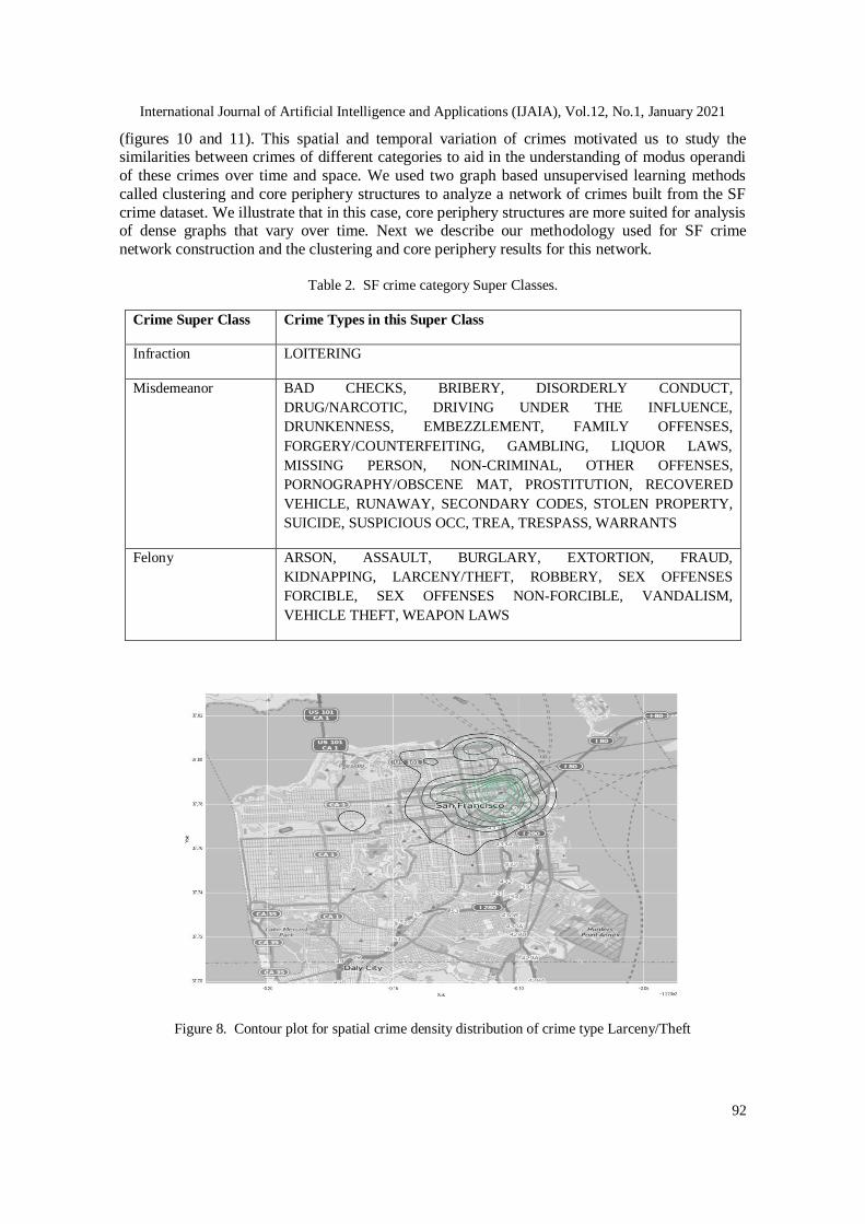
Given the raw data of crimes in SF (latitude and longitude), we used contour or density plots to

study the spread of different crime types. Two of these plots are presented in figures 8 and 9 for crime types larceny/theft and prostitution. This illustrates that crimes belonging to different

categories are localized to specific geographical areas in SF. We further plotted the normalized

crime counts for top 10 crimes to see some preliminary trends that how they vary with time


92

(figures 10 and 11). This spatial and temporal variation of crimes motivated us to study the similarities between crimes of different categories to aid in the understanding of modus operandi

of these crimes over time and space. We used two graph based unsupervised learning methods

called clustering and core periphery structures to analyze a network of crimes built from the SF

crime dataset. We illustrate that in this case, core periphery structures are more suited for analysis of dense graphs that vary over time. Next we describe our methodology used for SF crime

network construction and the clustering and core periphery results for this network.

Table 2. SF crime category Super Classes.

Crime Super Class Crime Types in this Super Class

Infraction LOITERING

Misdemeanor BAD CHECKS, BRIBERY, DISORDERLY CONDUCT,

DRUG/NARCOTIC, DRIVING UNDER THE INFLUENCE,

DRUNKENNESS, EMBEZZLEMENT, FAMILY OFFENSES,

FORGERY/COUNTERFEITING, GAMBLING, LIQUOR LAWS,

MISSING PERSON, NON-CRIMINAL, OTHER OFFENSES,

PORNOGRAPHY/OBSCENE MAT, PROSTITUTION, RECOVERED

VEHICLE, RUNAWAY, SECONDARY CODES, STOLEN PROPERTY,

SUICIDE, SUSPICIOUS OCC, TREA, TRESPASS, WARRANTS

Felony ARSON, ASSAULT, BURGLARY, EXTORTION, FRAUD,

KIDNAPPING, LARCENY/THEFT, ROBBERY, SEX OFFENSES

FORCIBLE, SEX OFFENSES NON-FORCIBLE, VANDALISM,

VEHICLE THEFT, WEAPON LAWS

Figure 8. Contour plot for spatial crime density distribution of crime type Larceny/Theft


93

Figure 9. Contour plot for spatial crime density distribution of crime type Prostitution

Figure 10. Variation of normalized crime count for top 10 crimes with years


94

Figure 11. Variation of normalized crime count for top 10 crimes with months

5.2. SF Crime Network Construction

Using the raw SF crime dataset, we constructed a graph G = (V, E) containing a vertex

corresponding to each of the 39 crime categories. The edge weights among different crime types

were constructed as the Tanimoto similarity [33] calculated between crime types using their geographical proximity in terms of shared zip codes. Tanimoto similarity is an advanced version

of both cosine similarity as well as Jaccard coefficient. It assumes the calculation of similarity

between vectors whose attributes may or may not be binary. In case the vectors are binary, it reduces to Jaccard coefficient. Given two crime types expressed as a vector of zip codes A and B,

the calculation of Tanimoto similarity between them is formalized as below.

We used a cutoff of 0.2 as the minimum similarity level required between any two crime categories to establish an edge between the two. This led to the construction of a weighted graph

of crime types with weights as Tanimoto similarities. Further, one graph was constructed for each

of the years 2005, 2010 and 2015 to analyze temporal variation of crime trends. In table 3, we list

the global graph clustering coefficient [34] of each of these constructed graphs for the three years. The global graph clustering coefficient is a ratio of the number of closed triplets to number

of all triplets in the graph. It gives a measure of density in the graph and lies between 0 and 1.

The high clustering coefficients for graphs of all years denote that all these graphs are very dense in nature.

Table 3. Model Evaluation results for SF crime category classification.

Year for which Graph is constructed Graph clustering coefficient

2005 0.943

2010 0.962

2015 0.849


95

5.3. Clustering Results for SF Crime Network

We used a state-of-the-art graph clustering algorithm called ClusterONE [35] to find clusters in

all the three SF Crime graphs for years 2005, 2010 and 2015. ClusterONE uses a greedy growth-based algorithm to grow clusters from seeds. We ran this algorithm with its default set of

parameters. The clustering results are shown in figure 12. In this figure, we can see that for the

years 2005 and 2010, all the nodes are being clustered into one big cluster. For the year 2015, all crime categories, except Sex Offences Non-Forcible, Bad Checks, Prostitution and Extortion

form one big cluster. This behavior is due to the high graph density or cliquish nature of the

graph. In all these graphs, the width of the edges has been drawn proportional to their similarity

value. It is to be noted that the edge similarity in these graphs varies amongst different crime types even when they are heavily connected in terms of topology.

Figure 12. Clustering results for the graph of SF crime types for the years 2005, 2010 and 2015 using

ClusterONE algorithm

Most of the graph clustering algorithms including ClusterONE [35] are good at identifying clusters which have high topological density in the graph and give less importance to the edge

weight-based density. Thus, as the next step, we used a graph core periphery finding algorithm

called CP-MKNN [36] [37] which uses both topological density as well as edge weight density in

a graph to extract very dense core clusters surrounded by sparse periphery clusters. A core-periphery algorithm based on the extension of ClusterONE clustering algorithm has been

proposed in [38], however, we decided to use the algorithm CP-MKNN as our choice of core

periphery algorithm because as demonstrated in [37], it is better than [38] in separating very dense cores from their sparser surroundings. Further, there is an advantage in using core

periphery structures over simple clusters to study graphs which vary over time because we can

study how different nodes move from cores to peripheries and vice versa. This movement of data


96

can really help us in studying change dynamics, which in the current case of crime analysis can help in understanding how crime patterns evolve over time.

5.4. Core Periphery Structures for SF Crime Network

In figure 13, we demonstrate the core periphery structures obtained by CP-MKNN [36] [37] for

the SF crime graphs for the years 2005, 2010 and 2015. We set input parameter K = 5.

Figure 13. Core Periphery structure results for the graph of SF crime types for the years 2005, 2010 and

2015 using CP-MKNN algorithm

Crimes like Vehicle Theft, Robbery and Fraud are always in the core cluster for the three years

2005, 2010 and 2015. Similarly, crimes like gambling and bribery are always in the periphery for

all the three years. There are some crime types which keep moving between the core and periphery clusters as the years pass by. For example, the crime type Family Offences is a

peripheral crime in 2005 and 2015 and became a core crime in the year 2010. The crime type

Disorderly Conduct was in periphery in the year 2005 but a part of core cluster for the years 2010

and 2015. This type of rich information about how crime patterns of different types of crimes change over

time with respect to each other can be highly beneficial for the law enforcement agencies to plan

their task forces for tackling anticipated crimes in different locations. Further, this information can also help in improving awareness among the general public about the changing nature of

crimes in their neighborhoods and help them be safe.

6. CONCLUSION

In this paper, we provide an extensive survey of trends of both supervised as well as unsupervised machine learning techniques that exist for the analysis of crimes. We use a dataset of crimes in


97

San Francisco to build supervised and unsupervised learning strategies to extract useful patterns and trends from it.

Specifically, for supervised algorithms, we proposed a novel way of feature extraction and built

models using Logistic Regression, Gradient Boosting, Naive Bayes and Random Forest. Based upon model evaluation results using F1 measure and Logloss score, Gradient Boosting and

Logistic Regression performed the best amongst all models. Moreover, Logistic Regression ran

much faster than the Gradient Boosting model. We further optimized this model by grouping crime categories into super classes: “Infraction”, “Misdemeanor” and “Felony”. Our modelling

and optimization workflow can be used as a general framework to predict crime categories/ super

classes in crime incident reports from various counties. This will be highly beneficial to the law enforcement agencies to do a risk analysis of different locations and times which are more prone

to crimes of different types.

In terms of unsupervised learning methodologies, we illustrated the use of core periphery structures to analyze patterns in crimes that vary over time and space. We provided examples of

how certain crimes move between cores and peripheries over time while some crime types

remain stable over years. Such a behavioral study of crimes can be extremely beneficial to the police to plan their task forces based upon the changing nature of crimes.

In a nutshell, we provide a demonstration of both supervised as well unsupervised strategies for the analysis of crimes in San Francisco. Our modelling and optimization workflow can be used as

a general framework to predict crime categories and analyze crime behaviors using crime

incident reports from various counties all over the world. Our approaches can be immensely

helpful in planning measures for crime prevention and raising awareness among the citizens of a county.

As a future research direction, for the unsupervised approach, we could calculate an advanced version of distance between two crime types taking into account the actual distance in miles

between the zip codes where crimes occur. This will improve upon the accuracy of the patterns

found using clustering and core periphery structures. This will further help us in finetuning the

clusters of crime which in turn can be used as super classes in the supervised learning optimization approach to improve its accuracy and applicability.

REFERENCES

[1] H. Adel, M. Salheen, and R. Mahmoud, “Crime in relation to urban design. Case study: the greater

Cairo region,” Ain Shams Eng. J., vol. 7, no. 3, pp. 925-938, 2016.

[2] S. Prabakaran, and S. Mitra, “Survey of analysis of crime detection techniques using data mining and

machine learning,” J. Physics: Conference Series, vol. 1000, no. 1, 2018.

[3] Q. Zhang, P. Yuan, Q. Zhou, and Z. Yang, “Mixed spatial-temporal characteristics based crime hot

spots prediction,” in IEEE 20th Intl. Conf. on Comput. Supported Cooperative Work in Des.

(CSCWD), 2016, pp. 97-101.

[4] E. Cesario, C. Catlett, and D. Talia, “Forecasting crimes using autoregressive models,” in IEEE 14th

Intl Conf on Dependable, Autonomic and Secure Computing, 14th Intl Conf on Pervasive Intelligence and Computing, 2nd Intl Conf on Big Data Intelligence and Computing and Cyber Science and

Technology Congress (DASC/PiCom/DataCom/CyberSciTech, 2016, pp.795-802.

[5] S. Kim, P. Joshi, P.S. Kalsi, and P. Taheri, “Crime analysis through machine learning,” in IEEE 9th

Annual Information Technology, Electronics and Mobile Communication Conference (IEMCON),

2018, pp. 415-420.

[6] N.O. Edoka, “Crime Incidents Classification Using Supervised Machine Learning Techniques:

Chicago,” PhD. Diss., Dublin, National College of Ireland, 2020.


98

[7] Y. Lamari, B. Freskura, A. Abdessamad, S. Eichberg, and S. de Bonviller, “Predicting Spatial Crime

Occurrences through an Efficient Ensemble-Learning Model.” ISPRS Int. Journal of Geo-Info, vol. 9,

no. 11, 2020.

[8] P. Cichosz, “Urban Crime Risk Prediction Using Point of Interest Data,” ISPRS Int. J. Geo-Info., vol.

9, no. 7, 2020. [9] J. Friedman, T. Hastie, and R. Tibshirani, The elements of statistical learning, vol. 1, no. 10, New

York: Springer series in statistics, 2001.

[10] K. Ramasubramanian, and A. Singh, "Machine Learning Model Evaluation." Machine Learning

Using R, Apress, Berkeley, CA, pp. 425-464, 2017.

[11] M. Vaquero Barnadas, “Machine learning applied to Crime Prediction,” BS thesis, Universitat

Politcnica de Catalunya, 2016.

[12] A. Chandrasekar, A. Sunder Raj, and P. Kumar. “Crime prediction and classification in San Francisco

City,” URL http://cs229. stanford.edu/proj2015/228_report.pdf, 2015.

[13] I. Pradhan, “Exploratory Data Analysis and Crime Prediction in San Francisco,” MS Project, San

Jose State University, USA, 2018.

[14] S. T. Ang, W. Wang, and S. Chyou, “San Francisco crime classification,” UCSD Project Report URL

https://cseweb.ucsd.edu/classes/wi15/cse255-a/reports/fa15/037.pdf, 2015. [15] Y. Abouelnaga, “San Francisco crime classification,” arXiv preprint arXiv:1607.03626, 2016.

[16] X. Wu, “An informative and predictive analysis of the San Francisco police department crime data,”

Ph.D. Diss., UCLA, 2016.

[17] “Classifications of Crime”, FindLaw, URL https://criminal.findlaw.com/criminal-law-

basics/classifications-of-crimes.html

[18] A. Sharma, and S. Sharma, “An intelligent analysis of web Crime Data using Data Mining,” Int. J.

Eng. and Innov. Tech. (IJEIT), vol. 2, no. 3, 2012.

[19] S. Kumar, and D. Toshniwal, “A Data Mining framework to analyze Road Accident Data,” J. Big

Data, vol. 2, no. 1, pp. 26, 2015.

[20] A. Joshi, A. Sai Sabitha, and T. Choudhury, “Crime analysis using K- means clustering,” in 3rd Int.

Conf. on Comp. Intell. and Net. (CINE), pp. 33-39, 2017. [21] B. Sivanagaleela, and S. Rajesh, “Crime Analysis and Prediction Using Fuzzy C-Means Algorithm,”

in 3rd Int. Conf. on Trends in Electronics and Informatics (ICOEI), 2019, pp. 595-599.

[22] C. Morselli, Inside criminal networks, vol. 8, New York, Springer, 2009.

[23] J. Xu, and H. Chen, “The topology of dark networks,” Communications of the ACM, vol. 51, no. 10,

pp. 58-65, 2008.

[24] F. Calderoni, “The structure of Drug Trafficking mafias: the Ndrangheta and cocaine,” Crime, law

and social change, vol. 58, no. 3, pp. 321-349, 2012.

[25] T. Divik, J. K. Dijkstra, and T. A. B. Snijders, “Structure, multiplexity, and centrality in a corruption

network: the Czech Rath affair,” Trends in Organized Crime, vol. 22, no. 3, pp. 274-297, 2019.

[26] A. Kantamneni, “Identifying Communities as Core-Periphery Structures in Evolving Networks,” MS

Thesis University of Cincinnati, 2016.

[27] G. Berlusconi, F. Calderoni, N. Parolini, N., M. Verani, and C. Piccardi, “Link prediction in criminal networks: A tool for criminal intelligence analysis,” PloS one, vol. 11, no. 4, 2016.

[28] E. Budur, S. Lee, and V. S. Kong, “Structural analysis of Criminal Network and predicting hidden

links using Machine Learning,” URL arXiv:1507.05739, 2015.

[29] “San Francisco Crime Data and Arrest Information”, Civic Hub, URL

https://www.civichub.us/ca/san-francisco/gov/police-department/crime-data.

[30] “San Francisco Crime Classification”, Kaggle, URL https://www.kaggle.com/c/sf-crime.

[31] “Police Department Incident Reports”, DataSF, URL https://data.sfgov. org/Public-Safety/Police-

Department-Incident-Reports-Historical-2003/tmnf-yvry/.

[32] N. Van Gheem, “Pyzipcode 1.0. 2016," URL https://pypi.org/project/pyzipcode/, 2016.

[33] A.A. Goshtasby, "Similarity and dissimilarity measures," Image registration. Springer, London, pp. 7-

66, 2012. [34] A. Barrat, M. Barthelemy, R. Pastor-Satorras and A. Vespignani, "The architecture of complex

weighted networks," in Proc. Nat. Acad. Sci., 2004, vol. 101, no. 11, pp. 3747-3752.

[35] T. Nepusz, H. Yu, and A. Paccanaro, “Detecting overlapping protein complexes in Protein-Protein

Interaction Networks,” Nature Methods, vol. 9, pp. 471-472, 2012.

[36] D. Sardana, “Analysis of Meso-scale Structures in Weighted Graphs,” PhD diss., University of

Cincinnati, 2017.


99

[37] D. Sardana and R. Bhatnagar, “Graph Algorithm to find Core Periphery structures using Mutual K-

Nearest Neighbors” Int. J. Art. Intell. (IJAIA): in press, 2021.

[38] D. Sardana and R. Bhatnagar, “Core Periphery structures in weighted graphs using Greedy growth,”

in IEEE/WIC/ACM International Conference on Web Intelligence, 2016, pp. 1-8.

AUTHORS Divya Sardana: Dr. Divya Sardana is a Senior Data Scientist at Teradata Corp.,

Santa Clara, CA, USA. She has a PhD in Computer Science from the University of Cincinnati, OH US. Her research targets development of scalable machine learning

and graph algorithms for the analysis of complex datasets in interdisciplinary

domains of data science such as Bioinformatics, Sociology and Smart

Manufacturing.

Shruti Marwaha: Dr Shruti Marwaha is a Research Engineer in the Department of

Cardiovascular Medicine. She received her PhD in Systems Biology and

Physiology from University of Cincinnati in 2015 and has been working as a

Bioinformatician with Stanford Center for Undiagnosed Diseases since 2016. Her

primary role involves analysis and management of genomics and immunology

data. She focuses on benchmarking variant callers, optimizing tools for variant

prioritization and analysis of single cell immune data.

Raj Bhatnagar: Dr. Raj Bhatnagar is a Professor at the department of EECS at

University of Cincinnati, Cincinnati, OH, USA. His research interests encompass

developing algorithms for data mining and pattern recognition problems in various

domains including Bioinformatics, Geographic Information Systems,

Manufacturing, and Business.

supervised and unsupervised machine learning methodologies

Documents

Transcript of supervised and unsupervised machine learning methodologies