UNIVERSITY OF CALIFORNIA,IRVINE

Towards Split Computing: Supervised Compression for Resource-Constrained EdgeComputing Systems

DISSERTATION

submitted in partial satisfaction of the requirementsfor the degree of

DOCTOR OF PHILOSOPHY

in Computer Science

by

Yoshitomo Matsubara

Dissertation Committee:Professor Marco Levorato, Chair

Professor Sameer SinghProfessor Stephan Mandt

2022

Portion of Chapter 3 © 2019 ACMPortion of Chapter 3 © 2020 IEEEPortion of Chapter 4 © 2020 ACMPortion of Chapter 4 © 2021 IEEEPortion of Chapter 5 © 2022 IEEE

All other materials © 2022 Yoshitomo Matsubara

DEDICATION

To my family.

ii

TABLE OF CONTENTS

Page

LIST OF FIGURES vi

LIST OF TABLES ix

ACKNOWLEDGMENTS x

VITA xii

ABSTRACT OF THE DISSERTATION xvi

1 Introduction 11.1 Motivation . . . . . . . . . . . . . . . . . . . . . . . . . . . . . . . . . . . . . 11.2 Dissertation Outline . . . . . . . . . . . . . . . . . . . . . . . . . . . . . . . 3

2 Related Work 52.1 Overview of Local, Edge, Split Computing and Early-Exit Models . . . . . . 5

2.1.1 Local and Edge Computing . . . . . . . . . . . . . . . . . . . . . . . 72.1.2 Split Computing . . . . . . . . . . . . . . . . . . . . . . . . . . . . . 8

2.2 Background of Deep Learning for Mobile Applications . . . . . . . . . . . . . 92.2.1 Lightweight Models . . . . . . . . . . . . . . . . . . . . . . . . . . . . 92.2.2 Model Compression . . . . . . . . . . . . . . . . . . . . . . . . . . . . 11

2.3 Split Computing: A Survey . . . . . . . . . . . . . . . . . . . . . . . . . . . 122.3.1 Split Computing without DNN Modification . . . . . . . . . . . . . . 122.3.2 The Need for Bottleneck Injection . . . . . . . . . . . . . . . . . . . . 162.3.3 Split Computing with Bottleneck Injection . . . . . . . . . . . . . . . 182.3.4 Split Computing with Bottlenecks: Training Methodologies . . . . . . 20

3 Introducing Bottlenecks 263.1 Background . . . . . . . . . . . . . . . . . . . . . . . . . . . . . . . . . . . . 263.2 Preliminary Discussion . . . . . . . . . . . . . . . . . . . . . . . . . . . . . . 283.3 Split Mimic DNN Models . . . . . . . . . . . . . . . . . . . . . . . . . . . . 293.4 Toy Experiments with Caltech 101 Dataset . . . . . . . . . . . . . . . . . . . 33

3.4.1 Model Accuracy . . . . . . . . . . . . . . . . . . . . . . . . . . . . . . 333.4.2 Inference Time Evaluation . . . . . . . . . . . . . . . . . . . . . . . . 353.4.3 Inference Time over Real-world Wireless Links . . . . . . . . . . . . . 38

iii

3.5 Extended Experiments with ImageNet dataset . . . . . . . . . . . . . . . . . 413.5.1 Training Speed . . . . . . . . . . . . . . . . . . . . . . . . . . . . . . 433.5.2 Bottleneck Channel . . . . . . . . . . . . . . . . . . . . . . . . . . . . 453.5.3 Inference Time Evaluation . . . . . . . . . . . . . . . . . . . . . . . . 46

3.6 Conclusion . . . . . . . . . . . . . . . . . . . . . . . . . . . . . . . . . . . . . 53

4 Towards Detection Tasks 544.1 CNN-based Object Detectors . . . . . . . . . . . . . . . . . . . . . . . . . . 544.2 Challenges and Approaches . . . . . . . . . . . . . . . . . . . . . . . . . . . 56

4.2.1 Mobile and Edge Computing . . . . . . . . . . . . . . . . . . . . . . . 564.2.2 Split Computing . . . . . . . . . . . . . . . . . . . . . . . . . . . . . 59

4.3 In-Network Neural Compression . . . . . . . . . . . . . . . . . . . . . . . . . 624.3.1 Background . . . . . . . . . . . . . . . . . . . . . . . . . . . . . . . . 624.3.2 R-CNN Model Analysis . . . . . . . . . . . . . . . . . . . . . . . . . 644.3.3 Bottleneck Positioning and Head Structure . . . . . . . . . . . . . . . 654.3.4 Loss Function . . . . . . . . . . . . . . . . . . . . . . . . . . . . . . . 684.3.5 Detection Performance Evaluation . . . . . . . . . . . . . . . . . . . . 694.3.6 Qualitative Analysis . . . . . . . . . . . . . . . . . . . . . . . . . . . 714.3.7 Bottleneck Quantization (BQ) . . . . . . . . . . . . . . . . . . . . . . 71

4.4 Neural Image Prefiltering . . . . . . . . . . . . . . . . . . . . . . . . . . . . . 734.5 Latency Evaluation . . . . . . . . . . . . . . . . . . . . . . . . . . . . . . . . 764.6 Conclusions . . . . . . . . . . . . . . . . . . . . . . . . . . . . . . . . . . . . 79

5 Supervised Compression for Split Computing 815.1 Introduction . . . . . . . . . . . . . . . . . . . . . . . . . . . . . . . . . . . . 815.2 Method . . . . . . . . . . . . . . . . . . . . . . . . . . . . . . . . . . . . . . 84

5.2.1 Overview . . . . . . . . . . . . . . . . . . . . . . . . . . . . . . . . . 845.2.2 Knowledge Distillation . . . . . . . . . . . . . . . . . . . . . . . . . . 855.2.3 Fine-tuning for Target Tasks . . . . . . . . . . . . . . . . . . . . . . . 88

5.3 Experiments . . . . . . . . . . . . . . . . . . . . . . . . . . . . . . . . . . . . 895.3.1 Baselines . . . . . . . . . . . . . . . . . . . . . . . . . . . . . . . . . . 895.3.2 Implementation of Our Entropic Student . . . . . . . . . . . . . . . . 915.3.3 Image Classification . . . . . . . . . . . . . . . . . . . . . . . . . . . . 925.3.4 Object Detection and Semantic Segmentation . . . . . . . . . . . . . 935.3.5 Bitrate Allocation of Latent Representations . . . . . . . . . . . . . . 965.3.6 Deployment Cost on Mobile Devices . . . . . . . . . . . . . . . . . . 965.3.7 End-to-End Prediction Latency Evaluation . . . . . . . . . . . . . . . 99

5.4 Conclusions . . . . . . . . . . . . . . . . . . . . . . . . . . . . . . . . . . . . 100

6 Conclusion 1016.1 Summary . . . . . . . . . . . . . . . . . . . . . . . . . . . . . . . . . . . . . 1016.2 Further Research Challenges . . . . . . . . . . . . . . . . . . . . . . . . . . . 103

Bibliography 105

iv

Appendix A - Chapter 3 - 116

Appendix B - Chapter 4 - 119

Appendix C - Chapter 5 - 122

v

LIST OF FIGURES

Page

2.1 Overview of (a) local, (b) edge, (c) split computing, and (d) early exiting:image classification as an example. . . . . . . . . . . . . . . . . . . . . . . . 6

2.2 Two different split computing approaches. . . . . . . . . . . . . . . . . . . . 132.3 Cross entropy-based training for bottleneck-injected deep neural network (DNN). 212.4 Knowledge distillation for bottleneck-injected DNN (student), using a pre-

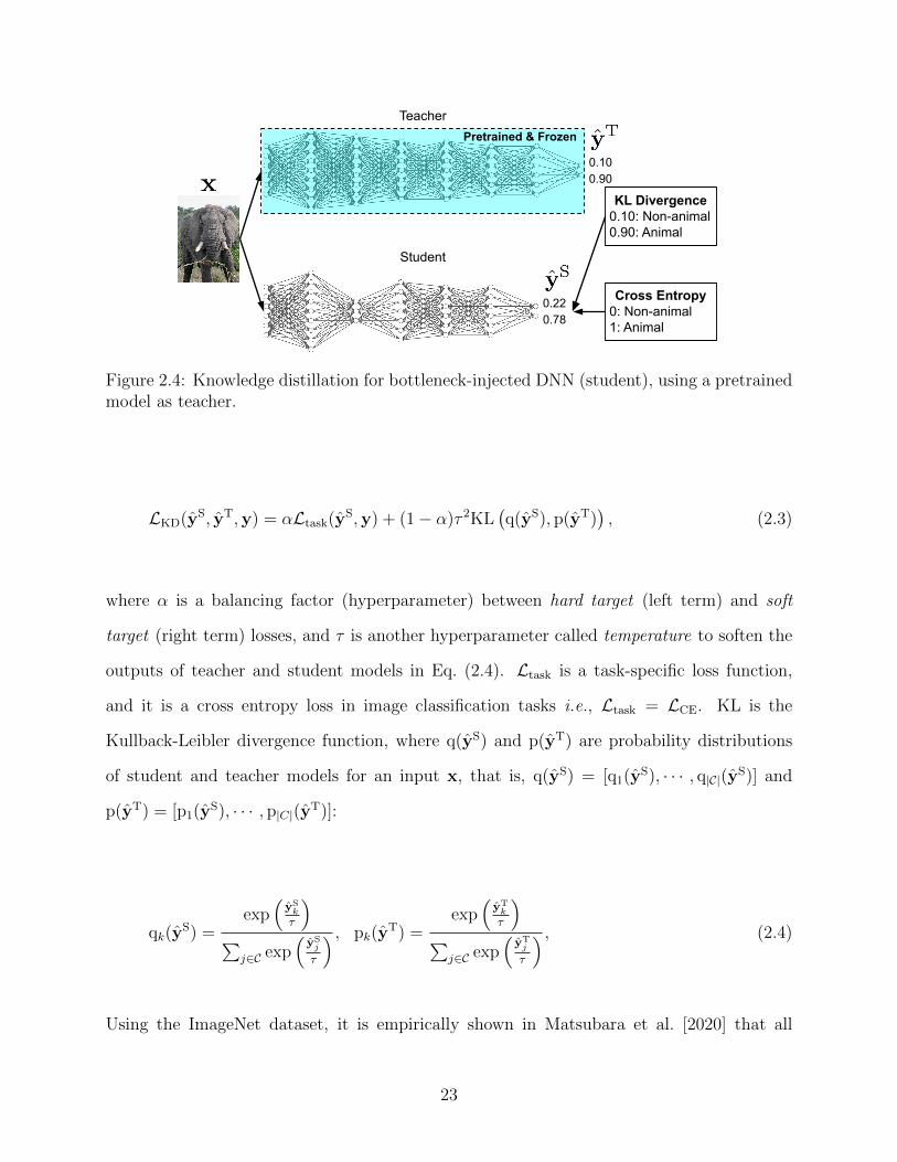
trained model as teacher. . . . . . . . . . . . . . . . . . . . . . . . . . . . . . 232.5 Reconstruction-based training to compress intermediate output (here z2) in

DNN by Autoencoder (AE) (yellow). . . . . . . . . . . . . . . . . . . . . . . 24

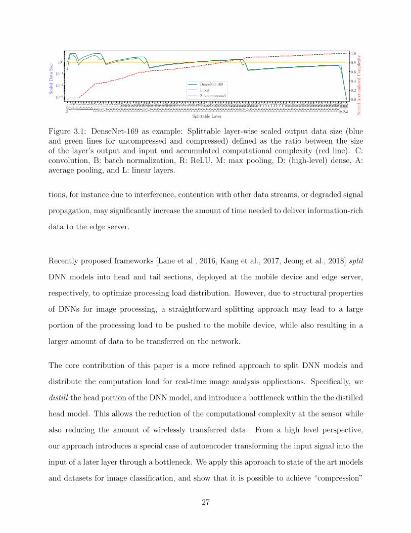
3.1 DenseNet-169 as example: Splittable layer-wise scaled output data size (blueand green lines for uncompressed and compressed) defined as the ratio betweenthe size of the layer’s output and input and accumulated computational com-plexity (red line). C: convolution, B: batch normalization, R: ReLU, M: maxpooling, D: (high-level) dense, A: average pooling, and L: linear layers. . . . 27

3.2 Illustration of head network distillation. . . . . . . . . . . . . . . . . . . . . . 303.3 The average and standard deviation of critical parameters . . . . . . . . . . 363.4 Capture-to-output delay and its components for different DNN configurations

as a function of the external traffic load. . . . . . . . . . . . . . . . . . . . . 393.5 Average capture-to-output delay over WiFi as a function of the external traffic

load. . . . . . . . . . . . . . . . . . . . . . . . . . . . . . . . . . . . . . . . . 403.6 Temporal series of capture-to-output per-frame delay over WiFi for (a) low,

(b) medium, and (c) high external traffic load. . . . . . . . . . . . . . . . . . 413.7 Capture-to-output delay and its components over emulated LTE network for

different DNN configurations as a function of external traffic load. . . . . . . 423.8 Illustrations of three different training methods. Naive: Naive training, KD:

Knowledge Distillation, HND: Head Network Distillation. . . . . . . . . . . . 433.9 Training speed and model accuracy for ImageNet dataset. . . . . . . . . . . 453.10 Relationship between bottleneck file size and validation accuracy with/without

bottleneck quantization (BQ). . . . . . . . . . . . . . . . . . . . . . . . . . . 473.11 Gains with respect to local computing. MD: mobile device, ES: edge server. . 493.12 Gains with respect to edge computing. MD: mobile device, ES: edge server. . 493.13 Gains with respect to local computing with MobileNet v2 in three different

configurations. . . . . . . . . . . . . . . . . . . . . . . . . . . . . . . . . . . . 50

vi

3.14 Local and edge computing delays for our split student head and tail modelsin different configurations. . . . . . . . . . . . . . . . . . . . . . . . . . . . . 51

3.15 Capture-to-output delay analysis for teacher and student models of DenseNet-201. LC: Local Computing, EC: Edge Computing, SC: Split Computing. . . 52

4.1 R-CNN with ResNet-based backbone. Blue modules are from its backbonemodel, and yellow modules are of object detection. C: Convolution, B: Batchnormalization, R: ReLU, M: Max pooling layers. . . . . . . . . . . . . . . . . 55

4.2 Layer-wise output tensor sizes of Faster and Mask R-CNNs scaled by inputtensor size (3× 800× 800). . . . . . . . . . . . . . . . . . . . . . . . . . . . . 61

4.3 Cumulative number of parameters in R-CNN object detection models. . . . . 654.4 Generalized head network distillation for R-CNN object detectors. Green

modules correspond to frozen blocks of individual layers of/from the teachermodel, and red modules correspond to blocks we design and train for thestudent model. L0-4 indicate high-level layers in the backbone. In this study,only backbone modules (orange) are used for training. . . . . . . . . . . . . . 66

4.5 Normalized bottleneck tensor size vs. mean average precision of Faster andMask R-CNNs with FPN. . . . . . . . . . . . . . . . . . . . . . . . . . . . . 69

4.6 Qualitative analysis. All figures are best viewed in pdf. . . . . . . . . . . . . 724.7 Neural filter (blue) to filter images with no object of interest. Only neural

filter’s parameters can be updated. . . . . . . . . . . . . . . . . . . . . . . . 744.8 Sample images in COCO 2017 training dataset. . . . . . . . . . . . . . . . . 754.9 Ratio of the total capture-to-output time T of local computing (LC) and

pure offloading (PO) to that of the proposed technique without (top)/with(bottom) a neural filter. . . . . . . . . . . . . . . . . . . . . . . . . . . . . . 77

4.10 Component-wise delays of original and our Keypoint R-CNNs in different datarates. LC: Local Computing, PO: Pure Offloading, SC: Split Computing,SCNF: Split Computing with Neural Filter . . . . . . . . . . . . . . . . . . . 79

5.1 Image classification with input compression (top) vs. our proposed super-vised compression for split computing (bottom). While the former approachfully reconstructs the image, our approach learns an intermediate compressiblerepresentation suitable for the supervised task. . . . . . . . . . . . . . . . . . 82

5.2 Proposed graphical model. Black arrows indicate the compression and decom-pression process in our student model. The dashed arrow shows the teacher’soriginal deterministic mapping. Colored arrows show the discriminative tailportions shared between student and teacher. . . . . . . . . . . . . . . . . . 85

5.3 Our two-stage training approach. Left: training the student model (bottom)with targets h and tail architecture obtained from teacher (top) (Section 5.2.2).Right: fine-tuning the decoder and tail portion with fixed encoder (Sec-tion 5.2.3). . . . . . . . . . . . . . . . . . . . . . . . . . . . . . . . . . . . . . 86

5.4 Rate-distortion (accuracy) curves of ResNet-50 as base model for ImageNet(ILSVRC 2012). . . . . . . . . . . . . . . . . . . . . . . . . . . . . . . . . . . 93

5.5 Rate-distortion (BBox mAP) curves of RetinaNet with ResNet-50 and FPNas base backbone for COCO 2017. . . . . . . . . . . . . . . . . . . . . . . . . 94

vii

5.6 Rate-distortion (Seg mIoU) curves of DeepLabv3 with ResNet-50 as base back-bone for COCO 2017. . . . . . . . . . . . . . . . . . . . . . . . . . . . . . . . 94

5.7 Bitrate allocations of latent representations z in neural image compressionand our entropic student models. Red and blue areas are allocated higherand lower bitrates, respectively (best viewed in PDF). It appears that thesupervised approach (right) allocates more bits to the information relevant tothe supervised classification goal. . . . . . . . . . . . . . . . . . . . . . . . . 97

viii

LIST OF TABLES

Page

2.1 Studies on split computing without architectural modifications. . . . . . . . 142.2 Statistics of image classification datasets in split computing studies . . . . . 172.3 Studies on split computing with bottleneck injection strategies. . . . . . . . . 20

3.1 Results on Caltech 101 dataset for DenseNet-169 models redesigned to intro-duce bottlenecks. . . . . . . . . . . . . . . . . . . . . . . . . . . . . . . . . . 31

3.2 Head network distillation results: mimic model with natural bottlenecks. . . 343.3 Head network distillation results: bottleneck-injected mimic model. . . . . . 343.4 Hardware specifications. . . . . . . . . . . . . . . . . . . . . . . . . . . . . . 353.5 Delay components and variances for DenseNet-201 in different network con-

ditions. . . . . . . . . . . . . . . . . . . . . . . . . . . . . . . . . . . . . . . . 383.6 Validation accuracy* [%] of student models trained with three different train-

ing methods. . . . . . . . . . . . . . . . . . . . . . . . . . . . . . . . . . . . . 443.7 Hardware specifications. . . . . . . . . . . . . . . . . . . . . . . . . . . . . . 48

4.1 Mean average precision (mAP) on COCO 2014 minival dataset and runningtime on a machine with an NVIDIA GeForce GTX TITAN X. . . . . . . . . 58

4.2 Inference time [sec/image] of Faster and Mask R-CNNs with different ResNetmodels and FPN. . . . . . . . . . . . . . . . . . . . . . . . . . . . . . . . . . 58

4.3 Pure offloading time [sec] (data rate: 5Mbps) of detection models with dif-ferent ResNet backbones on a high-end edge server with an NVIDIA GeForceRTX 2080 Ti. . . . . . . . . . . . . . . . . . . . . . . . . . . . . . . . . . . . 59

4.4 Performance of pretrained and head-distilled (3ch) models on COCO 2017validation datasets* for different tasks. . . . . . . . . . . . . . . . . . . . . . 70

4.5 Ratios of bottleneck (3ch) data size and tensor shape produced by head por-tion to input data. . . . . . . . . . . . . . . . . . . . . . . . . . . . . . . . . 73

5.1 Number of parameters in compression and classification models loaded onmobile device and edge server. Local (LC), Edge (EC), and Split computing(SC). . . . . . . . . . . . . . . . . . . . . . . . . . . . . . . . . . . . . . . . . 98

5.2 End-to-end latency to complete input-to-prediction pipeline for resource-constrainededge computing systems illustrated in Fig. 5.1, using RPI4/JTX2, LoRa andES. The breakdowns are available in the supplementary material. . . . . . . 99

ix

ACKNOWLEDGMENTS

First of all, I would love to thank my Ph.D. thesis advisor, Professor Marco Levorato, for hiscontinuous support and encouragement. Whenever I proposed research ideas to him, even ifsome of them were half-baked, he always tried to seek interesting points during discussion andencouraged me to give them a try e.g., introducing bottlenecks to DNNs. He also respectedmy research interests in other domains and gave me some freedom to pursue my personalresearch interests and collaborate with other groups while working on thesis research projectsin parallel. His flexibility saved me many times in research collaborations, and I learned alot from him while helping me in writing and presenting research papers. Since I have noteither taken his course or been familiar with his research areas, it must have been a little bitrisky for him to take me as a Ph.D. student of his group. I appreciate that he valued mymachine learning skills and bet on my potential through research collaboration. I was veryfortunate to have him as my Ph.D. thesis advisor. Without his support, this dissertationwould not have been possible.

I would like to thank Professor Sameer Singh, who introduced me to Professor Marco Lev-orato while looking for a thesis advisor. His research and courses showed me the powerof deep learning and helped me strengthen my skill set and background to conduct deeplearning-based research projects. Since my first year at UCI, he has helped me pursue someof my personal research interests during my Ph.D. program, such as discussing “blindness”of entities in scientific papers, Alexa Prize Socialbot Grand Challenge 3, and an NLP projectto combat COVID-19-related misinformation. I also learned a lot from his professional mind-set, and his technical skills inspired me to keep improving my skills. Without him, I wouldnot have either had a chance to work with Professor Marco Levorato or completed thisdissertation.

I would like to thank Professor Stephan Mandt for his critical advice and feedback frommachine learning and neural image compression perspectives. These were essential for meto elaborate our split computing approaches further and make breakthroughs in supervisedcompression for split computing. Without his support, Chapter 5 in this dissertation wouldnot have come true.

I am also grateful to the rest of the committee members for my Ph.D. candidacy exam,Professor Emre Neftci and Professor Lee Swindlehurst, for their constructive feedback andsuggestion. Besides, I would like to thank Professor Chen Li, my first Ph.D. advisor at UCI,for his big heart. When I revealed to him that I was more interested in machine learning, herespected my decision and helped me find different opportunities I could be more passionateabout. I was also fortunate to work on research projects closely with Dr. Davide Callegaro,Professor Sabur Baidya, Ruihan Yang, Robert L. Logan IV, Tamanna Hossain, Dr. ArjunaUgarte, Professor Sean D Young, Dheeru Dua, Dr. Alessandro Moschitti, Dr. Luca Soldaini,Dr. Thuy Vu, Eric Lind, Dr. Yoshitaka Ushiku, Dr. Naoya Chiba, Dr. Tatsunori Taniai,and Dr. Ryo Igarashi. It was also fun to regularly discuss research ideas and projects withthe members of the IASL group: Ali Tazarv, Anas Alsoliman, Peyman Tehrani, and SharonL.G. Contreras. I also would like to thank all my friends and colleagues at UCI, Yahoo Japan

x

Corporation, Slice Technologies, Amazon Alexa AI, and OMRON SINIC X Corporation.

During my Ph.D. program at UCI, I have been supported in part by the National ScienceFoundation (NSF) under Grant IIS-1724331 and Grant MLWiNS-2003237, DARPA underGrant HR00111910001, Alexa Prize, Intel Corporation, Google Cloud Platform researchcredits, and Donald Bren School of Information and Computer Sciences at UCI.

I also want to thank all my UCI table tennis club friends for the joyful time. For surviving inthe Ph.D. program, it was indispensable for me to make time to play table tennis with themeven when I was very busy with research projects. It was also memorable for me to win theNCTTA SoCal Divisional and West Regionals in 2018 and place 4th at the NCTTA NationalChampionship 2019 with Ray Yi, Hoi Man Chu, Newman Cheng, Krishnateja Avvari, andNeal Thakker.

Besides, I would like to thank Preston So, Nicholas Senturia, Zihao Yang, Brandon PT Davis,and Yoshimichi Nakatsuka for having long, fun times together in my SoCal life.

I also really appreciate the support from my family, Professor Haruhiko Nishimura, LateProfessor Toshiharu Samura, Professor Daisuke Sekimori, and Professor John C. Herbert,for pursuing my Ph.D. in the US.

Finally, I would love to thank Mai Kurosawa (now Mai Matsubara), my beloved wife, for herdecision to be part of my life, change her family name, and come to the US to pursue hercareer during this difficult time. I am very excited and looking forward to the next chaptersof our life.

xi

VITA

Yoshitomo Matsubara

EDUCATION

Doctor of Philosophy in Computer Science 2022University of California, Irvine Irvine, California

Master of Applied Informatics 2016University of Hyogo Hyogo, Japan

Bachelor of Engineering 2014Akashi National College of Technology Hyogo, Japan

PROFESSIONAL EXPERIENCE

Research Intern 2022OMRON SINIC X Corporation Tokyo, Japan

Applied Scientist Intern 2020–2021Amazon.com Services, Inc. Manhattan Beach, California

Applied Scientist Intern 2019Amazon.com Services, Inc. Manhattan Beach, California

Machine Learning Engineering Intern 2018Slice Technologies Inc. San Mateo, California

Contract Data Scientist 2017Yahoo Japan Corporation Osaka, Japan

Contract Data Scientist 2016Yahoo Japan Corporation Osaka, Japan

Special Intern 2015Yahoo Japan Corporation Osaka, Japan

Summer Intern 2014Recruit Holdings Co, Ltd. Tokyo, Japan

Spring Intern 2013Osaka University Osaka, Japan

Summer Intern 2012Hiroshima University Hiroshima, Japan

Summer Intern 2010University of Yamanashi Yamanashi, Japan

xii

TEACHING EXPERIENCE

Teaching Assistant 2016–2019University of California, Irvine Irvine, California

Teaching Assistant 2015–2016University of Hyogo Hyogo, Japan

Teaching Assistant 2012–2014Akashi National College of Technology Hyogo, Japan

VOLUNTEER EXPERIENCE

Virtual Conference VolunteerNeurIPS, ICML, ICLR 2020

ReceptionistSIGGRAPH Asia (Local committee) 2015

PROFESSIONAL SERVICE

Technical StaffACL Rolling Review 2021–2022

PC MemberNAACL 2021 Workshop on Scholarly Document Processing 2021

ReviewerICML 2022

ICC, ICLR, NeurIPS, WACV 2021

Internet of Things Journal, Journal of Data Semantics, 2020WACV, GLOBECOM

xiii

REFEREED JOURNAL PUBLICATIONS

Head Network Distillation: Splitting Distilled DeepNeural Networks for Resource-constrained Edge Com-puting Systems

2020

IEEE Access

REFEREED CONFERENCE PUBLICATIONS

Supervised Compression for Resource-ConstrainedEdge Computing Systems

Jan 2022

Proceedings of the IEEE/CVF Winter Conference on Applications of Computer Vision

torchdistill: A Modular, Configuration-Driven Frame-work for Knowledge Distillation

Jan 2021

International Workshop on Reproducible Research in Pattern Recognition at ICPR ’20

Neural Compression and Filtering for Edge-assistedReal-time Object Detection in Challenged Networks

Jan 2021

2020 25th International Conference on Pattern Recognition (ICPR)

COVIDLies: Detecting COVID-19 Misinformation onSocial Media

Nov 2021

Proceedings of the 1st Workshop on NLP for COVID-19 (Part 2) at EMNLP 2020

Optimal Task Allocation for Time-Varying Edge Com-puting Systems with Split DNNs

Dec 2020

GLOBECOM 2020 - 2020 IEEE Global Communications Conference

Split Computing for Complex Object Detectors: Chal-lenges and Preliminary Results

Sep 2020

Proceedings of the 4th International Workshop on Embedded and Mobile Deep Learning(EMDL ’20)

Citations Beyond Self Citations: Identifying Authors,Affiliations, and Nationalities in Scientific Papers

Jul 2020

Proceedings of the 8th Workshop on Mining Scientific Publications (WOSP ’20)

Reranking for Efficient Transformer-based Answer Se-lection

Jul 2020

Proceedings of the 43rd International ACM SIGIR Conference on Research and Devel-opment in Information Retrieval

Distilled Split Deep Neural Networks for Edge-AssistedReal-Time Systems

Oct 2019

Proceedings of the 2019 Workshop on Hot Topics in Video Analytics and IntelligentEdges (HotEdgeVideo ’19)

xiv

TECHNICAL REPORTS / PREPRINTS

Ensemble Transformer for Efficient and Accurate Rank-ing Tasks: an Application to Question Answering Sys-tems

2022

arXiv preprint arXiv:2201.05767

BottleFit: Learning Compressed Representations inDeep Neural Networks for Effective and Efficient SplitComputing

2022

arXiv preprint arXiv:2201.02693

Split Computing and Early Exiting for Deep LearningApplications: Survey and Research Challenges

2021

arXiv preprint arXiv:2103.04505

ZOTBOT: Using Reading Comprehension and Com-monsense Reasoning in Conversational Agents

2020

3rd Proceedings of Alexa Prize (Alexa Prize 2019)

SOFTWARE

sc2bench https://github.com/yoshitomo-matsubara/sc2-benchmark

A PyTorch-based supervised compression framework to facilitate reproducible studies onsupervised compression for split computing.

torchdistill https://github.com/yoshitomo-matsubara/torchdistill

A coding-free framework built on PyTorch for reproducible deep learning studies.

xv

ABSTRACT OF THE DISSERTATION

Towards Split Computing: Supervised Compression for Resource-Constrained EdgeComputing Systems

By

Yoshitomo Matsubara

Doctor of Philosophy in Computer Science

University of California, Irvine, 2022

Professor Marco Levorato, Chair

Mobile devices such as smartphones and autonomous vehicles increasingly rely on deep neu-

ral networks (DNNs) to execute complex inference tasks such as image classification and

speech recognition, among others. However, continuously executing the entire DNN on the

mobile device can quickly deplete its battery. Although task offloading to cloud/edge servers

may decrease the mobile device’s computational burden, erratic patterns in channel quality,

network, and edge server load can lead to a significant delay in task execution. Recently,

splitting DNN has been proposed to address such problems, where the DNN is split into two

sections to be executed on the mobile device and on the edge server, respectively. However,

the gain of naively splitting DNN models is limited since such approaches result in either

local computing or full offloading unless the DNN models have natural “bottlenecks”, which

are significantly small representations compared to the input data to the models.

Firstly, we explore popular DNN models in image classification tasks and point out that

such natural bottlenecks do not appear at early layers for most of the DNN models, thus

such naive splitting approaches would result in either local computing or full offloading. We

propose a framework to split DNNs and minimize capture-to-output delay in a wide range

of network conditions and computing parameters. Different from prior literature presenting

xvi

DNN splitting frameworks, we distill the architecture of the head DNN to reduce its com-

putational complexity and introduce a bottleneck, thus minimizing processing load at the

mobile device as well as the amount of wirelessly transferred data.

Secondly, since most prior work focuses on classification tasks and leaves the DNN struc-

ture unaltered, we put our focus on three different object detection tasks, which have more

complex goals than image classification tasks, and discuss split DNNs for the challenging

tasks. We propose techniques to (i) achieve in-network compression by introducing a bot-

tleneck layer in the early layers on the head model, and (ii) prefilter pictures that do not

contain objects of interest using a lightweight neural network. The experimental results show

that the proposed techniques represent an effective intermediate option between local and

edge computing in a parameter region where these extreme point solutions fail to provide

satisfactory performance.

Lastly, we introduce a concept of supervised compression for split computing and adopt ideas

from knowledge distillation and neural image compression to compress intermediate feature

representations more efficiently. Our supervised compression approach uses a teacher model

and a student model with a stochastic bottleneck and learnable prior for entropy coding.

We compare our approach to various compression baselines in three vision tasks and found

that it achieves better supervised rate-distortion performance while also maintaining smaller

end-to-end latency. We furthermore show that the learned feature representations can be

tuned to serve multiple downstream tasks. To facilitate studies of supervised compression

for split computing, we also propose a new tradeoff metric that considers not only data size

and model accuracy but also encoder size, which should be minimized for weak local devices.

xvii

Chapter 1

Introduction

1.1 Motivation

The field of deep learning has evolved at an impressive pace over the last few years [LeCun

et al., 2015], with new breakthroughs continuously appearing in domains such as computer

vision (CV) and natural language processing (NLP) – we refer to [Pouyanfar et al., 2018] for

a comprehensive survey on deep learning. For example, today’s state of the art DNNs (deep

neural networks) can classify thousands of images with unprecedented accuracy [Huang et al.,

2017], while bleeding-edge advances in deep reinforcement learning have shown to provide

near-human capabilities in a multitude of complex optimization tasks, from playing dozens of

Atari video games [Mnih et al., 2013] to winning games of Go against top-tier players [Silver

et al., 2017].

As deep learning-based models improve their predictive accuracy, mobile applications such

as speech recognition in smartphones [Deng et al., 2013, Hinton et al., 2012], real-time

unmanned navigation [Padhy et al., 2018] and drone-based surveillance [Singh et al., 2018,

Zhang et al., 2020] are increasingly using DNN to perform complex inference tasks. However,

1

state-of-the-art DNN models present computational requirements that cannot be satisfied

by the majority of the mobile devices available today. In fact, many state-of-the-art DNN

models for difficult tasks – such as computer vision and natural language processing – are

extremely complex. For instance, the EfficientDet [Tan et al., 2020] family offers the best

performance for object detection tasks. While EfficientDet-D7 achieves a mean average

precision (mAP) of 52.2%, it involves 52M parameters and will take seconds to be executed

on strong embedded devices equipped with GPUs such as the NVIDIA Jetson Nano and

Raspberry Pi. Notably, the execution of such complex models significantly increases energy

consumption. While lightweight models specifically designed for mobile devices exist [Tan

et al., 2019, Sandler et al., 2018], the reduced computational burden usually comes to the

detriment of the model accuracy. For example, compared to ResNet-152 [He et al., 2016],

the networks MnasNet [Tan et al., 2019] and MobileNetV2 [Sandler et al., 2018] present up

to 6.4% accuracy loss on the ImageNet dataset. YOLO-Lite [Redmon and Farhadi, 2018]

achieves a frame rate of 22 frames per second on some embedded devices but has mAP

of 12.36% on the COCO dataset [Lin et al., 2014]. To achieve 33.8% mAP on the COCO

dataset, even the simplest model in the EfficientDet family, EfficientDet-D0, requires 3 times

more FLOPs (2.5B) 1 than SSD-MobileNetV2 [Sandler et al., 2018] (0.8B FLOPs). While

SSD-MobileNetV2 is a lower-performance DNN specifically designed for mobile platforms

and can process up to 6 fps, its mAP on COCO dataset is 20% and keeping the model

running on a mobile device significantly increases power consumption. On the other hand,

due to excessive end-to-end latency, cloud-based approaches are hardly applicable in most

of the latency-constrained applications where mobile devices usually operate. Most of the

techniques we overview in the survey can be applied to both mobile device to edge server

and edge server to cloud offloading. For the sake of clarity, we primarily refer to the former

to explain the frameworks.

The severe offloading limitations of some mobile devices, coupled with the instability of the

1In Tan et al. [2020], FLOP denotes number of multiply-adds.

2

wireless channel (e.g., UAV network [Gupta et al., 2015]), imply that the amount of data

offloaded to edge should be decreased, while at the same time keep the model accuracy as

close as possible to the original. For this reason, split computing [Kang et al., 2017] strategies

have been proposed to provide an intermediate option between local computing and edge

computing. The key intuition behind split computing is similar to the one behind model

pruning [Han et al., 2016, Li et al., 2016, He et al., 2017b, Yang et al., 2017] and knowledge

distillation [Hinton et al., 2014, Kim and Rush, 2016, Mirzadeh et al., 2020] – since modern

DNNs are heavily over-parameterized [Yu et al., 2020, Yu and Principe, 2019], their accuracy

can be preserved even with substantial reduction in the number of weights and filters, and

thus representing the input with fewer parameters.

In split computing, a large DNN model is divided into head and tail models, which are

respectively executed by the mobile device and edge server. However, due to structural

properties of DNNs for image processing, a straightforward splitting approach may lead to

a large portion of the processing load to be pushed to the mobile device, while also resulting

in a larger amount of data to be transferred on the network. The outcome is an increase in

the overall time needed to complete the model execution.

1.2 Dissertation Outline

The rest of this dissertation is organized as follows:

• Chapter 2 describes overview of local, edge, and split computing and introduces back-

ground of deep learning for mobile applications. Following the contents, we share a

survey of related studies and highlight the need for bottlenecks in DNN models in order

to achieve efficient split computing.

• In Chapter 3, we analyze popular DNN models for image classification tasks and pro-

3

pose a framework to introduce artificial bottlenecks to existing DNN models and train

the bottleneck-injected models with low model training cost by distilling only head

portion of the original (teacher) models, named head network distillation (HND). We

also discuss total inference time (delay) of our baseline and proposed methods, using

real and simulated platforms.

• Chapter 4 is focused on object detection tasks and presents analysis of complex object

detection models and what makes split computing challenging for such models. To

address the problems, we propose generalized HND (GHND), that leverages multiple

intermediate feature representations from both teacher and student models to minimize

model accuracy loss with respect to the teacher model. Furthermore, we introduce a

lightweight neural filter to split computing paradigm, which is trained to detect images

containing no objects of interest so that we can terminate the inference for such images

at mobile device side and save communication delays.

• Chapter 5 introduces a concept of supervised compression and discusses the approaches

for split computing. Leveraging the ideas from neural image compression and knowl-

edge distillation, we propose Entropic Student, a new supervised compression approach

for split computing. We demonstrate that the proposed approach outperforms all the

strong baseline methods we consider in terms of rate-distortion tradeoff for 3 chal-

lenging tasks: image classification, object detection, and semantic segmentation for

ILSVRC 2012 (ImageNet) and COCO datasets respectively.

• Chapter 6 concludes this dissertation and opens up research challenges in split com-

puting for future work.

4

Chapter 2

Related Work

2.1 Overview of Local, Edge, Split Computing and Early-

Exit Models

In this section, we provide an overview of local, edge, and split computing models, which are

the main computational paradigms that will be discussed in the paper. Figure 2.1 provides

a graphical overview of the approaches.

All these techniques operate on a DNN model M(·) whose task is to produce the inference

output y from an input x. Typically, x is a high-dimensional variable, whereas the output

y has significantly lower dimensionality [Tishby and Zaslavsky, 2015]. Split computing ap-

proaches are contextualized in a setting where the system is composed of a mobile device

and an edge server interconnected via a wireless channel. The overall goal of the system is

to produce the inference output y from the input x acquired by the mobile device, by means

of the DNN y=M(x) under – possibly time varying – constraints on:

Resources: (i) the computational capacity (roughly expressed as number operations per

5

Mobile Device

Computing Capacity

(a)

Loca

l Co

mp

uti

ng

(b)

Edge

Co

mp

uti

ng

(c)

Split

Co

mp

uti

ng

Cloud/Edge Server

Computing Capacity

Prediction: “Rabbit”

Prediction: “Rabbit”

Sensor data

Intermediate output

Wireless Communication

Prediction: “Rabbit”

Com

pressor

Decom

pressor

(d)

Earl

y Ex

itin

g

Prediction: “Rabbit”

Intermediate output

Figure 2.1: Overview of (a) local, (b) edge, (c) split computing, and (d) early exiting: imageclassification as an example.

second) Cmd and Ces of the mobile device and edge server, respectively, (ii) the capacity ϕ,

in bits per second, of the wireless channel connecting the mobile device to the edge server;

Performance: (i) the absolute of average value of the time from the generation of x to the

availability of y, (ii) the degradation of the “quality” of the output y.

Split, edge, and local computing strategies strive to find suitable operating points with re-

spect to accuracy, end-to-end delay, and energy consumption, which are inevitably influenced

by the characteristics of the underlying system. It is generally assumed that the computing

and energy capacities of the mobile device are smaller than that of the edge server. As a

consequence, if part of the workload is allocated to the mobile device, then the execution

time increases while battery lifetime decreases. However, as explained later, the workload

executed by the mobile device may result in a reduced amount of data to be transferred

6

over the wireless channel, possibly compensating for the larger execution time and leading

to smaller end-to-end delays.

2.1.1 Local and Edge Computing

We start with an overview of local and edge computing. In local computing, the function

M(x) is entirely executed by the mobile device. This approach eliminates the need to

transfer data over the wireless channel. However, the complexity of the best performing

DNNs most likely exceeds the computing capacity and energy consumption available at the

mobile device. Usually, simpler models M(x) are used, such as MobileNet [Sandler et al.,

2018] and MnasNet [Tan et al., 2019] which often have a degraded accuracy performance.

Besides designing lightweight neural models executable on mobile devices, the widely used

techniques to reduce the complexity of models are knowledge distillation [Hinton et al.,

2014] and model pruning/quantization [Jacob et al., 2018, Li et al., 2018a] as introduced

in Section 2.2.2. Some of the techniques are also leveraged in split computing studies to

introduce bottlenecks without sacrificing model accuracy as will be described in the following

sections.

In edge computing (full offloading), the input x is transferred to the edge server, which

then executes the original model M(x). In this approach, which preserves full accuracy,

the mobile device is not allocated computing workload, but the full input x needs to be

transferred to the edge server. This may lead to an excessive end-to-end delay in degraded

channel conditions and erasure of the task in extreme conditions. A possible approach

to reduce the load imposed to the wireless channel, and thus also transmission delay and

erasure probability, is to compress the input x. We define, then, the encoder and decoder

models z=F (x) and x=G(z), which are executed at the mobile device and edge server,

respectively. The distance d(x, x) defines the performance of the encoding-decoding process

7

x=G(F (x)), a metric which is separate, but may influence, the accuracy loss of M(x) with

respect to M(x), that is, of the model executed with the reconstructed input with respect

to the model executed with the original input. Clearly, the encoding/decoding functions

increase the computing load both at the mobile device and edge server side. A broad range of

different compression approaches exists ranging from low-complexity traditional compression

(e.g., JPEG compression for images in edge computing [Nakahara et al., 2021]) to neural

compression models [Balle et al., 2017, 2018, Yang et al., 2020d]. We remark that while

the compressed input data e.g., JPEG objects, can reduce the data transfer time in edge

computing, those representations are designed to allow the accurate reconstruction of the

input signal. Therefore, these approaches may (i) decrease privacy as a “reconstructable”

representation is transferred to the edge server [Wang et al., 2020]; (ii) result in larger

amount of data to be transmitted over the channel compared to representation specifically

designed for the computing task as in bottleneck-based split computing as explained in the

following sections.

2.1.2 Split Computing

Split computing aims at achieving the following goals: (i) the computing load is distributed

across the mobile device and edge server; and (ii) establishes a task-oriented compression to

reduce data transfer delays. We consider a neural model M(·) with L layers, and define zℓ

the output of the ℓ-th layer. Early implementations of split computing select a layer ℓ and

divide the model M(·) to define the head and tail submodels zℓ=MH(x) and y=MT (zℓ),

executed at the mobile device and edge server, respectively. In early instances of split

computing, the architecture and weights of the head and tail model are exactly the same

as the first ℓ layers and last L− ℓ layers of M(·). This simple approach preserves accuracy

but allocates part of the execution of M(·) to the mobile device, whose computing power

is expected to be smaller than that of the edge server, so that the total execution time

8

may be larger. The transmission time of zℓ may be larger or smaller compared to that of

transmitting the input x, depending on the size of the tensor zℓ. However, we note that in

most relevant applications the size of zℓ becomes smaller than that of x only in later layers,

which would allocate most of the computing load to the mobile device. More recent split

computing frameworks introduce the notion of bottleneck to achieve in-model compression

toward the global task [Matsubara et al., 2019]. As formally described in the next section,

a bottleneck is a compression point at one layer in the model, which can be realized by

reducing the number of nodes of the target layer, and/or by quantizing its output. We note

that as split computing realizes a task-oriented compression, it guarantees a higher degree of

privacy compared to edge computing (EC). In fact, the representation may lack information

needed to fully reconstruct the original input data.

2.2 Background of Deep Learning for Mobile Applica-

tions

In this section, we provide an overview of recent approaches to reduce the computational

complexity of DNN models for resource-constrained mobile devices. These approaches can be

categorized into two main classes: (i) approaches that attempt to directly design lightweight

models and (ii) model compression.

2.2.1 Lightweight Models

From a conceptual perspective, The design of small deep learning models is one of the sim-

plest ways to reduce inference cost. However, there is a trade-off between model complexity

and model accuracy, which makes this approach practically challenging when aiming at high

model performance. The MobileNet series [Howard et al., 2017, Sandler et al., 2018, Howard

9

et al., 2019] is one among the most popular lightweight models for computer vision tasks,

where Howard et al. [2017] describes the first version MobileNetV1. By using a pair of

depth-wise and point-wise convolution layers in place of standard convolution layers, the

design drastically reduces model size, and thus computing load. Following this study, San-

dler et al. [2018] proposed MobileNetV2, which achieves an improved accuracy. The design

is based on MobileNetV1 [Howard et al., 2017], and uses the bottleneck residual block, a

resource-efficient block with inverted residuals and linear bottlenecks. Howard et al. [2019]

presents MobileNetV3, which further improves the model accuracy and is designed by a

hardware-aware neural architecture search [Tan et al., 2019] with NetAdapt [Yang et al.,

2018]. The largest variant of MobileNetV3, MobileNetV3-Large 1.0, achieves a comparable

accuracy of ResNet-34 [He et al., 2016] for the ImageNet dataset, while reducing by about

75% the model parameters.

While many of the lightweight neural networks are often manually designed, there are also

studies on automating the neural architecture search (NAS) [Zoph and Le, 2017]. For in-

stance, Zoph et al. [2018] designs a novel search space through experiments with the CIFAR-

10 dataset [Krizhevsky, 2009], that is then scaled to larger, higher resolution image datasets

such as the ImageNet dataset [Russakovsky et al., 2015], to design their proposed model:

NASNet. Leveraging the concept of NAS, some studies design lightweight models in a

platform-aware fashion. Dong et al. [2018] proposes the Device-aware Progressive Search

for Pareto-optimal Neural Architectures (DDP-Net) framework, that optimizes the network

design with respect to two objectives: device-related (e.g., inference latency and memory

usage) and device-agnostic (e.g., accuracy and model size) objectives. Similarly, Tan et al.

[2019] propose an automated mobile neural architecture search (MNAS) method and design

the MnasNet models by optimizing both model accuracy and inference time.

10

2.2.2 Model Compression

A different approach to produce small DNN models is to “compress” a large model. Model

pruning and quantization [Han et al., 2015, 2016, Jacob et al., 2018, Li et al., 2020] are

the dominant model compression approaches. The former removes parameters from the

model, while the latter uses fewer bits to represent them. In both these approaches, a large

model is trained first and then compressed, rather than directly designing a lightweight

model followed by training. In Jacob et al. [2018], the authors empirically show that their

quantization technique leads to an improved tradeoff between inference time and accuracy on

MobileNet [Howard et al., 2017] for image classification tasks on Qualcomm Snapdragon 835

and 821 compared to the original, float-only MobileNet. For what concerns model pruning,

Li et al. [2017a], Liu et al. [2021] demonstrates that it is difficult for model pruning itself

to accelerate inference while achieving strong performance guarantees on general-purpose

hardware due to the unstructured sparsity of the pruned model and/or kernels in layers.

Knowledge distillation [Bucilua et al., 2006, Hinton et al., 2014] is another popular model

compression method. While model pruning and quantization make trained models smaller,

the concept of knowledge distillation is to provide outputs extracted from the trained model

(called “teacher”) as informative signals to train smaller models (called “student”)to improve

the accuracy of predesigned small models. Thus, the goal of the process is that of distilling

knowledge of a trained teacher model into a smaller student model for boosting accuracy

of the smaller model without increasing model complexity. For instance, Ba and Caruana

[2014] proposes a method to train small neural networks by mimicking the detailed behavior

of larger models. The experimental results show that models trained by this mimic learning

method achieve performance close to that of deeper neural networks on some phoneme

recognition and image recognition tasks. The formulation of some knowledge distillation

methods will be described in Section 2.3.4.

11

2.3 Split Computing: A Survey

This section discusses existing state of of the art in split computing. Figure 2.2 illustrates the

existing split computing approaches. They can be categorized into either (i) without network

modification or (ii) with bottleneck injection. We first present split computing approaches

without DNN modification in Section 2.3.1. We then discuss the motivations behind the

introduction of split computing with bottlenecks in Section 2.3.2, which are then discussed

in details in Section 2.3.3. Since the latter require specific training procedures, we devote

Section 2.3.4 to their discussion.

2.3.1 Split Computing without DNN Modification

In this class of approaches, the architecture and weights of the head MH(·) and tail MT (·)

models are exactly the same as the first ℓ layers and last L− ℓ layers of M(·). To the best

of our knowledge, Kang et al. [2017] proposed the first split computing approach (called

“Neurosurgeon”), which searches for the best partitioning layer in a DNN model for mini-

mizing total (end-to-end) latency or energy consumption. Formally, inference time in split

computing is the sum of processing time on mobile device, delay of communication between

mobile device and edge server, and the processing time on edge server.

Interestingly, their experimental results show that the best partitioning (splitting) layers in

terms of energy consumption and total latency for most of the considered models result in

either their input or output layers. In other words, deploying the whole model on either

a mobile device or an edge server (i.e., local computing or EC) would be the best option

for such DNN models. Following the work by Kang et al. [2017], the research communities

explored various split computing approaches mainly focused on CV tasks such as image

classification. Table 2.1 summarizes the studies on split computing without architectural

12

Figure 2.2: Two different split computing approaches.

modifications.

Jeong et al. [2018] used this partial offloading approach as a privacy-preserving way for

computation offloading to blind the edge server to the original data captured by client.

Leveraging neural network quantization techniques, Li et al. [2018a] discussed best splitting

point in DNN models to minimize inference latency, and showed quantized DNN models

did not degrade accuracy comparing to the (pre-quantized) original models. Choi and Bajic

[2018] proposed a feature compression strategy for object detection models that introduces a

quantization/video-coding based compressor to the intermediate features in YOLO9000 [Red-

mon and Farhadi, 2017].

Eshratifar et al. [2019a] propose JointDNN for collaborative computation between mobile

device and cloud, and demonstrate that using either local computing only or cloud com-

puting only is not an optimal solution in terms of inference time and energy consumption.

Different from [Kang et al., 2017], they consider not only discriminative deep learning models

(e.g., classifiers), but also generative deep learning models and autoencoders as benchmark

models in their experimental evaluation. Cohen et al. [2020] introduce a technique to code

13

Table 2.1: Studies on split computing without architectural modifications.

Work Task(s) Dataset(s) Model(s) Metrics Code

Kang et al. [2017]

Image classificationSpeech recognition

Part-of-speech taggingNamed entity recognition

Word chunking

N/A(No task-specific metrics)

AlexNetVGG-19DeepFaceLeNet-5Kaldi

SENNA

D, E, L

Li et al. [2018b] Image classificationN/A

(No task-specific metrics)AlexNet C, D

Jeong et al. [2018] Image classificationN/A

(No task-specific metrics)

GoogLeNetAgeNet

GenderNetD, L

Li et al. [2018a] Image classification ImageNet

AlexNetVGG-16ResNet-18GoogLeNet

A, D, L

Choi and Bajic [2018] Object detection VOC 2007 YOLO9000 A, C, D, L

Eshratifar et al. [2019a]Image classificationSpeech recognition

N/A(No task-specific metrics)

AlexNetOverFeat

NiNVGG-16ResNet-50

D, E, L

Zeng et al. [2019] Image classification CIFAR-10 AlexNet A, D, L

Cohen et al. [2020]Image classificationObject detection

ImageNet (2012)COCO 2017

VGG-16ResNet-50YOLOv3

A, D

Pagliari et al. [2020]Natural language inferenceReading comprehension

Sentiment analysis

N/A(No task-specific metrics)

RNNs E, L

Itahara et al. [2021] Image classification CIFAR-10 VGG-16 A, D

A: Model accuracy, C: Model complexity, D: Transferred data size, E: Energy consumption, L: Latency,T: Training cost

14

the output of the head portion in a split DNN to a wide range of bit-rates, and demonstrate

the performance for image classification and object detection tasks. Pagliari et al. [2020] first

discuss the collaborative inference for simple recurrent neural networks, and their proposed

scheme is designed to automatically select the best inference device for each input data in

terms of total latency or end-device energy. Itahara et al. [2021] use dropout layers [Srivas-

tava et al., 2014] to emulate a packet loss scenario rather than for the sake of compression

and discuss the robustness of VGG-based models [Simonyan and Zisserman, 2015] for split

computing.

While only a few studies in Table 2.1 heuristically choose splitting points [Choi and Bajic,

2018, Cohen et al., 2020], most of the other studies [Kang et al., 2017, Li et al., 2018b, Jeong

et al., 2018, Li et al., 2018a, Eshratifar et al., 2019a, Zeng et al., 2019, Pagliari et al., 2020]

in Table 2.1 analyze various types of cost (e.g., computational load and energy consumption

on mobile device, communication cost, and/or privacy risk) to partition DNN models at

each of their splitting points. Based on the analysis, performance profiles of the split DNN

models are derived to inform selection. Concerning metrics, many of the studies in Table 2.1

do not discuss task-specific performance metrics such as accuracy. This is in part because

the proposed approaches do not modify the input or intermediate representations in the

models (i.e., the final prediction will not change). On the other hand, Li et al. [2018a], Choi

and Bajic [2018], Cohen et al. [2020] introduce lossy compression techniques to intermediate

stages in DNN models, which more or less affect the final prediction results. Thus, discussing

trade-off between compression rate and task-specific performance metrics would be essential

for such studies. As shown in the table, such trade-off is discussed only for CV tasks, and

many of the models considered in such studies have weak performance compared with state-

of-the-art models and complexity within reach of modern mobile devices. Specific to image

classification tasks, most of the models considered in the studies listed in Table 2.1 are more

complex and/or the accuracy is comparable to or lower than that of lightweight baseline

models such as MobileNetV2 [Sandler et al., 2018] and MnasNet [Tan et al., 2019]. Thus, in

15

future work, more accurate models should be considered to discuss the performance trade-off

and further motivate split computing approaches.

2.3.2 The Need for Bottleneck Injection

While Kang et al. [2017] empirically show that executing the whole model on either mobile

device or edge server would be best in terms of total inference and energy consumption for

most of their considered DNN models, their proposed approach find the best partitioning

layers inside some of their considered CV models (convolutional neural networks (CNNs))

to minimize the total inference time. There are a few trends observed from their experi-

mental results: (i) communication delay to transfer data from mobile device to edge server

is a key component in split computing to reduce total inference time; (ii) all the neural

models they considered for NLP tasks are relatively small (consisting of only a few layers),

that potentially resulted in finding the output layer is the best partition point (i.e., local

computing) according to their proposed approach; (iii) similarly, not only DNN models they

considered (except VGG [Simonyan and Zisserman, 2015]) but also the size of the input data

to the models (See Table 2.2) are relatively small, which gives more advantage to EC (fully

offloading computation). In other words, it highlights that complex CV tasks requiring large

(high-resolution) images for models to achieve high accuracy such as ImageNet and COCO

datasets would be essential to discuss the trade-off between accuracy and execution metrics

to be minimized (e.g., total latency, energy consumption) for split computing studies. The

key issue is that naive split computing approaches like Kang et al. [2017] rely on the existence

of natural bottlenecks – that is, intermediate layers whose output zℓ tensor size is smaller

than the input – inside the model. Without such natural bottlenecks in the model, naive

splitting approaches would fail to improve performance in most settings [Barbera et al., 2013,

Guo, 2018].

16

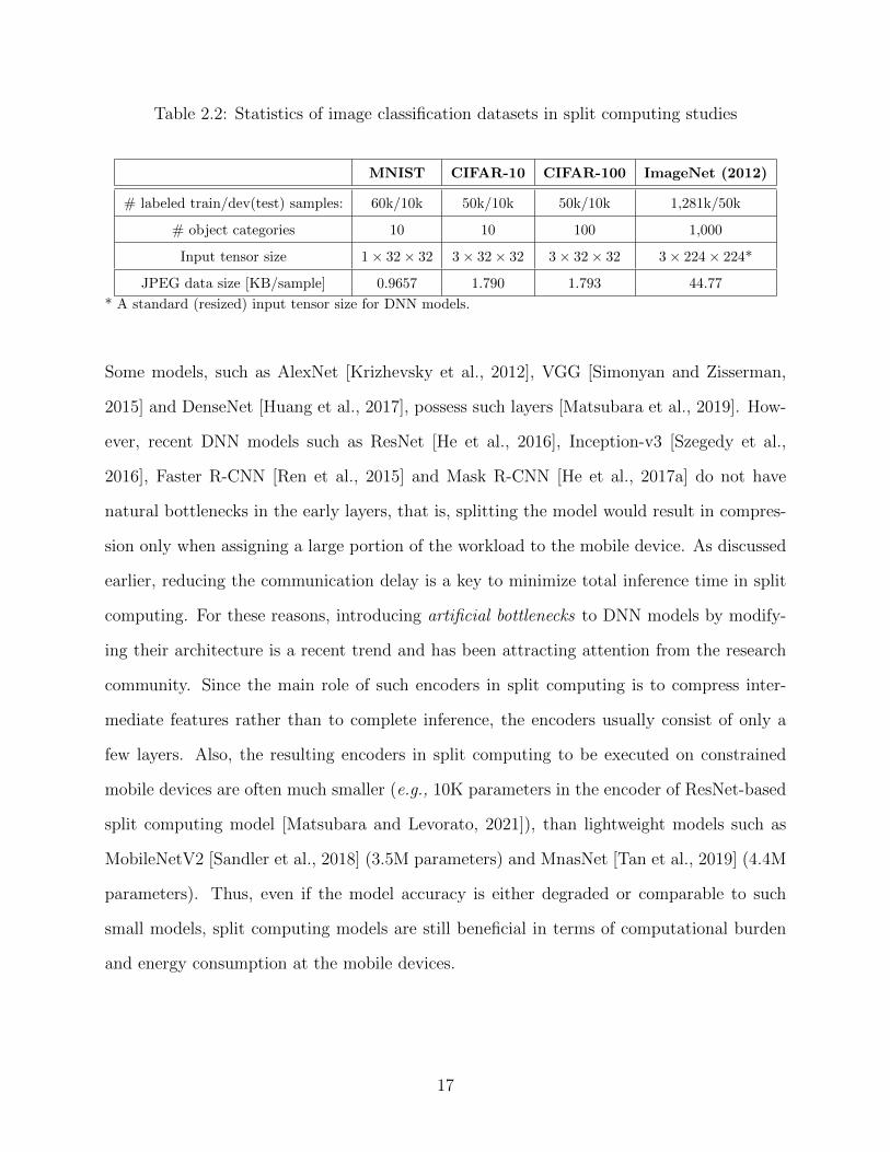
Table 2.2: Statistics of image classification datasets in split computing studies

MNIST CIFAR-10 CIFAR-100 ImageNet (2012)

# labeled train/dev(test) samples: 60k/10k 50k/10k 50k/10k 1,281k/50k

# object categories 10 10 100 1,000

Input tensor size 1× 32× 32 3× 32× 32 3× 32× 32 3× 224× 224*

JPEG data size [KB/sample] 0.9657 1.790 1.793 44.77

* A standard (resized) input tensor size for DNN models.

Some models, such as AlexNet [Krizhevsky et al., 2012], VGG [Simonyan and Zisserman,

2015] and DenseNet [Huang et al., 2017], possess such layers [Matsubara et al., 2019]. How-

ever, recent DNN models such as ResNet [He et al., 2016], Inception-v3 [Szegedy et al.,

2016], Faster R-CNN [Ren et al., 2015] and Mask R-CNN [He et al., 2017a] do not have

natural bottlenecks in the early layers, that is, splitting the model would result in compres-

sion only when assigning a large portion of the workload to the mobile device. As discussed

earlier, reducing the communication delay is a key to minimize total inference time in split

computing. For these reasons, introducing artificial bottlenecks to DNN models by modify-

ing their architecture is a recent trend and has been attracting attention from the research

community. Since the main role of such encoders in split computing is to compress inter-

mediate features rather than to complete inference, the encoders usually consist of only a

few layers. Also, the resulting encoders in split computing to be executed on constrained

mobile devices are often much smaller (e.g., 10K parameters in the encoder of ResNet-based

split computing model [Matsubara and Levorato, 2021]), than lightweight models such as

MobileNetV2 [Sandler et al., 2018] (3.5M parameters) and MnasNet [Tan et al., 2019] (4.4M

parameters). Thus, even if the model accuracy is either degraded or comparable to such

small models, split computing models are still beneficial in terms of computational burden

and energy consumption at the mobile devices.

17

2.3.3 Split Computing with Bottleneck Injection

This class of models can be described as composed of 3 sections: ME, MD and MT . We

define zℓ|x as the output of the ℓ-th layer of the original model given the input x. The

concatenation of the ME and MD models is designed to produce a possibly noisy version

zℓ|x of zℓ|x, which is taken as input by MT to produce the output y, on which the accuracy

degradation with respect to y is measured. The models ME, MD function as specialized

encoders and decoders in the form zℓ=MD(ME(x)), where ME(x) produces the latent

variable z. In worlds, the two first sections of the modified model transform the input x

into a version of the output of the ℓ-th layer via the intermediate representation z, thus

functioning as encoder/decoder functions. The model is split after the first section, that is,

ME is the head model, and the concatenation of MD and MT is the tail model. Then, the

tensor z is transmitted over the channel. The objective of the architecture is to minimize

the size of z to reduce the communication time while also minimizing the complexity of ME

(that is, the part of the model executed at the – weaker – mobile device) and the discrepancy

between y and y. The layer between ME and MD is the injected bottleneck.

Table 2.3 summarizes split computing studies with bottleneck injected strategies. To the

best of our knowledge, the papers in [Eshratifar et al., 2019b] and [Matsubara et al., 2019]

were the first to propose altering existing DNN architectures to design relatively small bot-

tlenecks at early layers in DNN models, instead of introducing compression techniques (e.g.,

quantization, autoencoder) to the models, so that communication delay (cost) and total in-

ference time can be further reduced. Following these studies, Hu and Krishnamachari [2020]

introduce bottlenecks to MobileNetV2 [Sandler et al., 2018] (modified for CIFAR datasets)

in a similar way for split computing, and discuss end-to-end performance evaluation. Choi

et al. [2020] combine multiple compression techniques such as quantization and tiling besides

convolution/deconvolution layers, and design a feature compression approach for object de-

tectors. Similar to the concept of bottleneck injection, Shao and Zhang [2020] find that

18

over-compression of intermediate features and inaccurate communication between comput-

ing devices can be tolerated unless the prediction performance of the models are significantly

degraded by them. Also, Jankowski et al. [2020] propose introducing a reconstruction-based

bottleneck to DNN models, which is similar to the concept of BottleNet [Eshratifar et al.,

2019b]. A comprehensive discussion on the delay/complexity/accuracy tradeoff can be found

in [Yao et al., 2020, Matsubara et al., 2020].

These studies are all focused on image classification. Other computer CV tasks present

further challenges. For instance, state of the art object detectors such as R-CNN models

have more narrow range of layers that we can introduce bottlenecks due to the network

architecture, which has multiple forward paths to forward outputs from intermediate layers

to feature pyramid network (FPN) [Lin et al., 2017a]. The head network distillation training

approach – discussed later in this section – was used in Matsubara and Levorato [2021] to

address some of these challenges and reduce the amount of data transmitted over the channel

by 94% while degrading mAP (mean average precision) loss by 1 point. Assine et al. [2021]

introduce bottlenecks to the EfficientDet-D2 [Tan et al., 2020] object detector, and apply the

training method based on the generalized head network distillation [Matsubara and Levorato,

2021] and mutual learning [Yang et al., 2020b] to the modified model. Following the studies

on split computing for resource-constrained edge computing systems [Matsubara et al., 2019,

2020, Yao et al., 2020], Sbai et al. [2021] introduce autoencoder to small classifiers and train

them on a subset of the ImageNet dataset in a similar manner. These studies discuss the

trade-off between accuracy and memory size on mobile devices, considering communication

constraints based 3G and LoRa technologies [Samie et al., 2016].

19

Table 2.3: Studies on split computing with bottleneck injection strategies.

Work Task(s) Dataset(s) Base Model(s) Training Metrics Code

Eshratifar et al. [2019b] Image classification miniImageNetResNet-50VGG-16

CE-based A, D, L

Hu and Krishnamachari [2020] Image classification CIFAR-10/100 MobileNetV2 CE-based A, D, L

Choi et al. [2020] Object detection COCO 2014 YOLOv3 Reconstruct. A, D

Shao and Zhang [2020] Image classification CIFAR-100ResNet-50VGG-16

CE-based(Multi-stage)

A, C, D

Jankowski et al. [2020] Image classification CIFAR-100 VGG-16CE + L2

(Multi-stage)A, C, D

Yao et al. [2020]Image classificationSpeech recognition

ImageNet (2012)LibriSpeech

ResNet-50Deep Speech

Reconst.+ KD

A, D, E, L, T Link*

Assine et al. [2021] Object detection COCO 2017 EfficientDet GHND-based A, C, D Link

Sbai et al. [2021] Image classificationSubset of ImageNet

(700 classes)MobileNetV1

VGG-16Reconst.+ KD

A, C, D

A: Model accuracy, C: Model complexity, D: Transferred data size, E: Energy consumption, L: Latency, T: Training cost* The repository is incomplete and lacks of instructions to reproduce the reported results for vision and speech datasets.

2.3.4 Split Computing with Bottlenecks: Training Methodologies

Given that recent split computing studies with bottleneck injection strategies result in more

or less accuracy loss comparing to the original models (i.e., without injected bottlenecks),

various training methodologies are used and/or proposed in such studies. Some of the train-

ing methods are designed specifically for architectures with injected bottlenecks. We now

summarize the differences between the various training methodologies used in recent split

computing studies.

We recall that x and y are an input (e.g., an RGB image) and the corresponding label

(e.g., one-hot vector) respectively. Given an input x, a DNN model M returns its output

y = M(x) such as class probabilities in classification task. Each of the L layers of model

M can be either low-level (e.g., convolution [LeCun et al., 1998], batch normalization [Ioffe

and Szegedy, 2015]), ReLU [Nair and Hinton, 2010]) or high-level layers (e.g., residual block

in ResNet [He et al., 2016] and dense block in DenseNet [Huang et al., 2017]) which are

composed by multiple low-level layers. M(x) is a sequence of the L layer functions fj’s, and

the jth layer transforms zj−1, the output from the previous (j − 1)th layer:

20

0.220.78

Cross Entropy0: Non-animal1: Animal

Figure 2.3: Cross entropy-based training for bottleneck-injected DNN.

zj =

x j = 0

fj(zj−1, θj) 1 ≤ j < L ,

fL(zL−1, θL) = M(x) = y j = L

(2.1)

where θj denotes the jth layer’s hyperparameters and parameters to be optimized during

training.

Cross entropy-based training

To optimize parameters in a DNN model, we first need to define a loss function and update

the parameters by minimizing the loss value with an optimizer such as stochastic gradient

descent and Adam [Kingma and Ba, 2015] during training. In image classification, a standard

method is to train a DNN model M in an end-to-end manner using the cross entropy like

many of the studies [Eshratifar et al., 2019b, Hu and Krishnamachari, 2020, Matsubara et al.,

2020] in Table 2.3. For simplicity, here we focus on the categorical cross entropy and suppose

c ≡ y is the correct class index given a model input x. Given a pair of x and c, we obtain

the model output y = M(x), and then the (categorical) cross entropy loss is defined as

LCE(y, c) = − log

(exp (yc)∑j∈C exp (yj)

), (2.2)

21

where yj is the class probability for the class index j, and C is a set of considered classes

(c ∈ C).

As shown in Eq. (2.2), the loss function used in cross entropy-based training methods are

used as a function of the final output y, and thus are not designed for split computing

frameworks. While Eshratifar et al. [2019b], Hu and Krishnamachari [2020], Shao and Zhang

[2020] use the cross entropy to train bottleneck-injected DNN models, Matsubara et al. [2020]

empirically show that these methodologies cause a larger accuracy loss in complex tasks such

as ImageNet dataset [Russakovsky et al., 2015] compared to other more advanced techniques,

including knowledge distillation.

Knowledge distillation

Complex DNN models are usually trained to learn parameters for discriminating between

a large number of classes (e.g., 1, 000 in ImageNet dataset), and often overparameterized.

Knowledge distillation (KD) Li et al. [2014], Ba and Caruana [2014], Hinton et al. [2014]

is a training scheme to address this problem, and trains a DNN model (called “student”)

using additional signals from a pretrained DNN model (called “teacher” and often larger

than the student). In standard cross entropy-based training – that is, using “hard targets”

(e.g., one-hot vectors) – we face a side-effect that the trained models assign probabilities to

all of the incorrect classes. From the relative probabilities of incorrect classes, we can see

how large models tend to generalize.

As illustrated in Fig. 2.4, by distilling the knowledge from a pretrained complex model

(teacher), a student model can be more generalized and avoid overfitting to the training

dataset, using the outputs of the teacher model as “soft targets” in addition to the hard

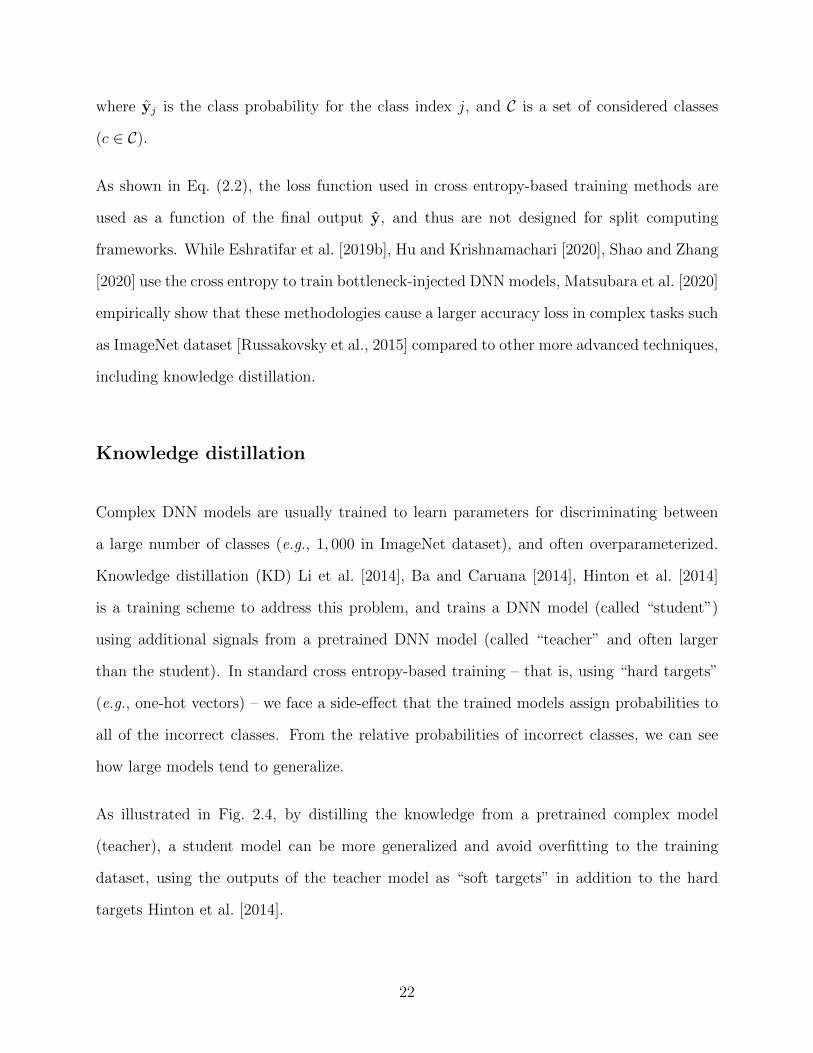
targets Hinton et al. [2014].

22

0.220.78

Cross Entropy0: Non-animal1: Animal

0.100.90

KL Divergence0.10: Non-animal0.90: Animal

Pretrained & FrozenTeacher

Student

Figure 2.4: Knowledge distillation for bottleneck-injected DNN (student), using a pretrainedmodel as teacher.

LKD(yS, yT,y) = αLtask(y

S,y) + (1− α)τ 2KL(q(yS), p(yT)

), (2.3)

where α is a balancing factor (hyperparameter) between hard target (left term) and soft

target (right term) losses, and τ is another hyperparameter called temperature to soften the

outputs of teacher and student models in Eq. (2.4). Ltask is a task-specific loss function,

and it is a cross entropy loss in image classification tasks i.e., Ltask = LCE. KL is the

Kullback-Leibler divergence function, where q(yS) and p(yT) are probability distributions

of student and teacher models for an input x, that is, q(yS) = [q1(yS), · · · , q|C|(yS)] and

p(yT) = [p1(yS), · · · , p|C|(y

T)]:

qk(yS) =

exp(

ySk

τ

)∑

j∈C exp(

ySj

τ

) , pk(yT) =

exp(

yTk

τ

)∑

j∈C exp(

yTj

τ

) , (2.4)

Using the ImageNet dataset, it is empirically shown in Matsubara et al. [2020] that all

23

Reconstruction Loss : AE input : AE output

Autoencoder (AE)

Figure 2.5: Reconstruction-based training to compress intermediate output (here z2) in DNNby AE (yellow).

the considered bottleneck-injected student models trained with their teacher models (origi-

nal models without injected bottlenecks) consistently outperform those trained without the

teacher models. This result matches a widely known trend in knowledge distillation reported

in Ba and Caruana [2014]. However, similar to cross entropy, the knowledge distillation is

still not aware of bottlenecks we introduce to DNN models and may result in significant

accuracy loss as suggested by Matsubara et al. [2020].

Reconstruction-based training

As illustrated in Fig. 2.5, Choi et al. [2020], Jankowski et al. [2020], Yao et al. [2020], Sbai

et al. [2021] inject AE models into existing DNN models, and train the injected components

by minimizing the reconstruction error. First manually an intermediate layer in a DNN

model (say its jth layer) is chosen, and the output of the jth layer zj is fed to the encoder

fenc whose role is to compress zj. The encoder’s output zenc is a compressed representation,

i.e., bottleneck to be transferred to edge server and the following decoder fdec decompresses

the compressed representation and returns zdec. As the decoder is designed to reconstruct

zj, its output zdec should share the same dimensionality with zj. Then, the injected AE are

trained by minimizing the following reconstruction loss:

24

LRecon. (zj) = ∥zj − fdec (fenc (zj; θenc) ; θdec) + ϵ∥mn , (2.5)

= ∥zj − zdec + ϵ∥mn ,

where ∥z∥mn denotes mth power of n-norm of z, and ϵ is an optional regularization constant.

For example, Choi et al. [2020] setm = 1, n = 2 and ϵ = 10−6, and Jankowski et al. [2020] use

m = n = 1 and ϵ = 0. Inspired by the idea of knowledge distillation [Hinton et al., 2014], Yao

et al. [2020] also consider additional squared errors between intermediate feature maps from

models with and without bottlenecks as additional loss terms like generalized head network

distillation [Matsubara and Levorato, 2021] described later. While Yao et al. [2020] shows

high compression rate with small accuracy loss by injecting encoder-decoder architectures to

existing DNN models, such strategies [Choi et al., 2020, Jankowski et al., 2020, Yao et al.,

2020, Sbai et al., 2021] increase computational complexity as a result. Suppose the encoder

and decoder consist of Lenc and Ldec layers respectively, then the total number of layers in

the altered DNN model is L+ Lenc + Ldec.

25

Chapter 3

Introducing Bottlenecks

3.1 Background

Deep Neural Networks (DNNs) achieve state of the art performance in a broad range of

classification, prediction and control problems. However, the computational complexity of

DNN models has been growing together with the complexity of the problems they solve. For

instance, within the image classification domain, LeNet5, proposed in 1998 [LeCun et al.,

1998], consists of 7 layers only, whereas DenseNet, proposed in 2017 [Huang et al., 2017],

has 713 low-level layers. Despite the advances in embedded systems of the recent years,

the execution of DNN models in mobile platforms is becoming increasingly problematic,

especially for mission critical or time sensitive applications, where the limited processing

power and energy supply may degrade the response time of the system and its lifetime.

Offloading data processing tasks to edge servers [Satyanarayanan et al., 2009, Bonomi et al.,

2012], that is, compute-capable devices located at the network edge, has been proven to be

an effective strategy to relieve the computation burden at the mobile devices and reduce

capture-to-classification output delay in some applications. However, poor channel condi-

26

Input

C:1

B:2

R:3

M:4

D:5

D:6

D:7

D:8

D:9

D:10

B:11

R:12

C:13

A:14

D:15

D:16

D:17

D:18

D:19

D:20

D:21

D:22

D:23

D:24

D:25

D:26

B:27

R:28

C:29

A:30

D:31

D:32

D:33

D:34

D:35

D:36

D:37

D:38

D:39

D:40

D:41

D:42

D:43

D:44

D:45

D:46

D:47

D:48

D:49

D:50

D:51

D:52

D:53

D:54

D:55

D:56

D:57

D:58

D:59

D:60

D:61

D:62

B:63

R:64

C:65

A:66

D:67

D:68

D:69

D:70

D:71

D:72

D:73

D:74

D:75

D:76

D:77

D:78

D:79

D:80

D:81

D:82

D:83

D:84

D:85

D:86

D:87

D:88

D:89

D:90

D:91

D:92

D:93

D:94

D:95

D:96

D:97

D:98

B:99

R:100

A:101

L:102

Splittable Layer

10−3

10−2

10−1

100

ScaledDataSize

DenseNet-169

Input

Zip-compressed0.0

0.2

0.4

0.6

0.8

1.0

ScaledAccumulatedCom

plexity

Figure 3.1: DenseNet-169 as example: Splittable layer-wise scaled output data size (blueand green lines for uncompressed and compressed) defined as the ratio between the sizeof the layer’s output and input and accumulated computational complexity (red line). C:convolution, B: batch normalization, R: ReLU, M: max pooling, D: (high-level) dense, A:average pooling, and L: linear layers.

tions, for instance due to interference, contention with other data streams, or degraded signal

propagation, may significantly increase the amount of time needed to deliver information-rich

data to the edge server.

Recently proposed frameworks [Lane et al., 2016, Kang et al., 2017, Jeong et al., 2018] split

DNN models into head and tail sections, deployed at the mobile device and edge server,

respectively, to optimize processing load distribution. However, due to structural properties

of DNNs for image processing, a straightforward splitting approach may lead to a large

portion of the processing load to be pushed to the mobile device, while also resulting in a

larger amount of data to be transferred on the network.

The core contribution of this paper is a more refined approach to split DNN models and

distribute the computation load for real-time image analysis applications. Specifically, we

distill the head portion of the DNN model, and introduce a bottleneck within the the distilled

head model. This allows the reduction of the computational complexity at the sensor while

also reducing the amount of wirelessly transferred data. From a high level perspective,

our approach introduces a special case of autoencoder transforming the input signal into the

input of a later layer through a bottleneck. We apply this approach to state of the art models

and datasets for image classification, and show that it is possible to achieve “compression”

27

up to 1% of the input signal with a complexity 95% smaller than the original head model.

3.2 Preliminary Discussion

We consider state of the art DNN models for image classification. Specifically, we study:

DenseNet-169, -201 [Huang et al., 2017], ResNet-152 [He et al., 2016] and Inception-v3 [Szegedy

et al., 2016]. We train and test the models on the CalTech 101 [Fei-Fei et al., 2006] and

ImageNet [Russakovsky et al., 2015] datasets.

We remark that in split DNN strategies, the overall inference time is the sum of three

components: the time needed to execute the head and tail portions of the model – τhead

and τtail respectively – and the time to wirelessly transfer the output of the head model’s

last layer to the edge server τdata. We assume that the edge server has a high computation

capacity, and seek strategies reducing computation load at the mobile device – that is, the

complexity of the head network portion – and the amount of data to be transferred. Pure

edge computing can be interpreted as an extreme point of splitting, where the head portion

is composed of 0 layers, and τdata is the time to transfer the input image.

Figure 3.1 shows the scaled size of data to be transferred, expressed as percentage compared

to the input size, and the scaled accumulated complexity (number of operations performed

up to that layer) for the layers of DenseNet-169 where the model can be split. The trend

illustrates the issue: the output of the layers becomes perceivably smaller than the input

only in later layers. Thus, reducing τdata would require the – weaker – mobile device to

execute most of the model, possibly resulting in an overall larger τhead+τdata compared to

transferring the input image and executing the head portion at the edge server (pure offload-

ing). Importantly, most early layers have an output size larger than the input, and reaching

the first point where a reasonable compression is achieved – approximately 33% of the input

28

at layer 30 – corresponds to execute 60% of the total operations composing the whole DNN.

The second candidate layer to split the DNN is layer 66, where the output is approximately

21% of the input after an accumulated complexity of 91% of the whole model. Then, the

output size slowly increases until the very last layers. Reported in the figure, standard Zip

compression allows to reduce the data size of the DNN layers – or of the input – without any

loss of classification accuracy. However, almost no compression gain is achieved in “natural”

splitting points, and compression does not provide a real advantage.

Intuitively, these trends do not allow an effective splitting strategy in asymmetric systems

where the mobile device has a much smaller computational power compared to the edge

server. Additionally, an increase in the time needed to transfer data penalizes splitting with

respect to pure offloading. Thus, we contend that achieving an advantageous balance between

computation at a weaker device and communication over a possibly impaired wireless channel

necessitates modifications to the DNN architecture.

3.3 Split Mimic DNN Models

Our overall objective is to reduce the complexity of head models while minimizing the amount

of data transferred from the mobile device to the edge server. To this aim, we use two

recent tools: network distillation and the introduction of bottlenecks. Figure 3.2 illustrates

the modifications in the overall architecture of the DNN. In the experiments shown in this

section, the datasets are randomly split into training, validation and test datasets with a

ratio 8:1:1, respectively.

Bottlenecks have been recently theoretically shown to promote the DNNs to learn optimal

representations [Achille and Soatto, 2018], thus achieving compression within the model.

However, as reported in Table 3.1, making more aggressive the “natural” bottlenecks di-

29

Teacher

model

Stu

dent

model

Mimicked output

Splitting point in the head-distilled model

Figure 3.2: Illustration of head network distillation.

rectly in the original DNN model resulted in accuracy degradation even for relatively mild

compression rates. Moreover, some models, such as Inception-v3, do not present any candi-

date splitting point. Thus, more substantial modifications to the architecture are needed.

Network Distillation We propose to “shrink” the head model using network distilla-

tion [Li et al., 2014, Ba and Caruana, 2014, Urban et al., 2017, Anil et al., 2018], a recently

proposed technique to train small “student” networks approximating the output of larger

“teacher” models. Interestingly, Ba and Caruana [2014] show that student models trained

on “soft-labeled” dataset (output of their teacher models) significantly improve prediction

performance compared to student models trained on the original (“hard-labeled”) training

dataset only, i.e., without a teacher model. However, distilling entire DNN models for image

analysis to fit the capabilities of mobile devices could degrade their performance. As an

indication of this issue, effective small models such as MobileNetV2 [Sandler et al., 2018], a

lower complexity model designed to run on mobile devices, achieve a test accuracy of about

30

Table 3.1: Results on Caltech 101 dataset for DenseNet-169 models redesigned to introducebottlenecks.

Metrics \ 1st Conv *64 channels 8 channels 4 channels

Test accuracy [%] 84.5 83.9 80.5

Data size [%] 133 16.7 8.33

* number of channels in the original model

71% on CalTech 101 – a significantly worse performance compared to the models built in this

work. Additionally, MobileNet models have a significantly higher complexity – 46% increase

– placed at the mobile device compared to our head models.

In the problem setting we considered, the key advantages of using distillation are: (a)

properly distilled models often give comparable performance while reducing the number

of parameters used in the model and, thus, computation complexity. This will allow us

to create efficient distilled head models mimicking the original head network; (b) student

models often avoid overfitting during distillation as the soft-target from a teacher model

has a regularization effect [Ba and Caruana, 2014, Urban et al., 2017]; and (c) the smaller

number of nodes in student models results in a natural reduction of the data to be transferred

to the edge server if the splitting point is positioned inside the student model. Moreover,

as we will demonstrate later in this section, the more manageable structure of our student

models will allow the creation of aggressive bottlenecks.

Figure 3.2 illustrates the student-teacher distillation approach in the considered split DNN

configuration. At first, we split a pretrained DNN model into head (red) and tail (blue)

networks. Taking DenseNet-169 as an example, Fig. 3.1 allows the identification of the

natural bottleneck points in the original DNN model at the 1st, 2nd and 3rd average pooling

layers (layer number 14, 30 and 66).

The original pretrained DNN (consisting of L layers) is used as a starting point, whose

architecture (in the head part) is simplified to design a bottleneck-injected student model.

31

As only the teacher’s head portion is altered, the tail portion of the student model is identical

to that of the original teacher model with respect to architecture and the same pretrained

parameters can be maintained. Thus, head network distillation requires only the first layers

of the teacher and student models in training session as the student head model fShead will

be trained to mimic behavior of teacher’s head model fThead given an input x. Specifically,

we use Adam [Kingma and Ba, 2015] to train the student head model by minimizing the

following loss:

LHND(x) = ∥fShead(x)− fThead(x)∥2, (3.1)

where fShead and fThead are sequences of the first LShead and LT

head layers in student and teacher

models (LShead ≪ LS, and LT

head ≪ L ), respectively.

fThead(x) and fShead(x) are (often 3D-shaped) outputs of teacher and student head models

respectively, and fThead(x) is fixed given x and treated as a target intermediate feature map to

train the student head model fShead(x). Thus, our objective is to train the student model so

that the model can mimic its teacher model i.e. fShead(x) ≈ fThead(x) given the input x. In the

training process, we feed exactly the same input x into both the teacher and student models.

The teacher model has been already trained with the dataset, and its model parameters are

fixed. We update the student head model’s parameters such that its output fShead(x) is close

to fThead(x) by minimizing the loss function defined in Eq. (3.1).

32

3.4 Toy Experiments with Caltech 101 Dataset

3.4.1 Model Accuracy

Table 3.2 reports the accuracy, data size and complexity reduction using the proposed tech-

niques on DenseNet-169 and -201 at different splitting points. The mobile device (MD)

complexity reduction granted by the student model is computed as(1 − CS

CT

)× 100, where

CS and CT indicate the computational complexity of the student and teacher models, re-

spectively. Note these mimic models do not alter the amount of data transferred to the edge

server, as they latch to the original tail network at the bottlenecks already present in the

original model. In the tables, we list the output size of the 1st bottleneck in the original

models as reference. The head network distillation successfully reduces complexity of the

head model while keeping accuracy comparable to the original one irrespective of the split-

ting point. A slight degradation is perceivable when the student model includes the layers up

to the 3rd bottleneck of DenseNet-169, possibly indicating the compression of an excessive

portion of the network.

Bottleneck Injection The student models developed earlier reduce complexity, but still

produce an output size which is, at the minimum, around 30% of the input at the 3rd splitting

point. We now devise distilled student models where we introduce aggressive bottlenecks

to further reduce the amount of data transferred to the edge server. To this aim, in all the

considered DNNs, we artificially inject bottlenecks at the very early stages of the student

models. We emphasize that, thus, the splitting point is inside the student model, rather

than at its end, and the edge server will need to execute a portion of the student model.

Table 3.3 shows even when a DNN model (e.g., ResNet-152 and Inception-v3 models) has no

bottleneck point, our proposed approach enables the introduction of an aggressive bottleneck

33

Table 3.2: Head network distillation results: mimic model with natural bottlenecks.

DenseNet-169 Mimic

Metrics Original 1st SP 2nd SP 3rd SP

Test accuracy [%] 84.5 84.0 84.3 83.8

Data size [%] 66.7 66.7 33.3 20.8

MD complexity 1.28 ×109 2.29 ×108 2.53 ×108 1.30 ×109

(Reduction [%]) (0.00) (82.1) (88.0) (58.2)

DenseNet-201 Mimic

Metrics Original 1st SP 2nd SP 3rd SP

Test accuracy [%] 85.2 84.2 84.1 84.3

Data size [%] 66.7 66.7 33.3 29.2

MD complexity 1.28 ×109 2.29 ×108 2.53 ×108 1.51 ×109

(Reduction [%]) (0.00) (82.1) (88.0) (62.4)

Table 3.3: Head network distillation results: bottleneck-injected mimic model.

Mimicked model

Metrics DenseNet-169 DenseNet-201 ResNet-152 Inception-v3

Test accuracy [%] 83.3 (-1.2) 84.1 (-1.1) 83.2 (-1.1) 85.7 (-0.8)

Data size [%] 1.68 1.68 1.68 1.53

MD complexity 1.22 ×108 1.22 ×108 1.22 ×108 2.11 ×108

(Reduction [%]) (94.2) (94.2) (95.5) (84.4)

within the student model, so that by splitting the student model at that point we reduce

both computational complexity on mobile device and transferred data size. Compared to

the original models, we achieve a dramatic reduction in both complexity and output data

size with at most about 1% accuracy drop. The mimic model has an output size of 1−2% of

the input, obtained with a number of operations reduced by up to 95.5% compared to the

original head model.

Due to the extensive time needed to train the models, we only report preliminary results

based on the ImageNet dataset, presenting a more complex classification task due to its

size and the large number of classes. The distilled mimic model with bottleneck achieved

a data size reduction of 11% of the input, and a complexity reduction of 94%. This result

demonstrates that head model compression is possible even in difficult tasks.

34

Table 3.4: Hardware specifications.

Computer Processor Speed [GHz] RAM [GB]

RPI3b+ ARM Cortex A53 (quad-core) 1.2 1

UP Board Intel Atom x5-Z8350 (quad-core) 1.92 4

Jetson TX2ARM Cortex-A57 (quad-core)

+ NVIDIA Denver2 (dual-core)2.0 8

Laptop Intel i7-6700HQ (octa-core) 2.6 16

3.4.2 Inference Time Evaluation

We now evaluate complete processing pipelines over a distributed mobile device-edge server

system, which is the main focus of this contribution. To this aim, we implement the necessary

modules for processing, communication and synchronization within a custom distributed

pipeline. The results we present in the following explore an ample range of hardware (see

Table 3.4) and communication data rates to provide an evaluation of the interesting interplay

between the delay components. The original model is DenseNet-201, and local computing

and pure edge computing Org. (MD) and Org. (ES) are compared with the mimic model

with bottleneck (Mimic w/B) at the first splitting point.

The set of plots in Fig. 3.3 reports the gain – expressed as the ratio between the capture-

to-output time T of the Mimic w/B model and that of pure offloading (Org. ES )/local

processing at the mobile device (Org. MD) – as a function of data rate in different hard-

ware/network configurations. Figures 3.3 (a) and (b) show the gain trends for different

mobile devices when the edge server is the laptop. Intuitively, the larger the data rate, the

smaller the gain with respect to Org. ES, as the reduction in τdata granted by the bottleneck

decreases compared to the possible disadvantage of executing part of the processing on a

slower platform. Note that slower mobile devices emphasize the latter, to the point that

the slowest considered embedded device (Raspberry Pi 3) has a gain smaller than 1, that is,

the proposed technique leads to larger capture-to-output time compared to Org. ES if the

35

0 2 4 6 8 10

Data Rate [Mbps]

0

2

4

6

8

10

12

14

Gainw.r.t.edge

proc. RPI3b

UpBoard

Jetson

(a) Gain w.r.t. full offloading,Laptop as ES.

0 2 4 6 8 10

Data Rate [Mbps]

0

10

20

30

40

50

Gainw.r.t.localproc.

RPI3b

UpBoard

Jetson

(b) Gain w.r.t. local processing, Laptop as ES.

0 2 4 6 8 10

Data Rate [Mbps]

0.0

0.5

1.0

1.5

2.0

2.5

3.0

3.5

Gainw.r.t.edge

proc. UpBoard

Jetson

Laptop

(c) Gain w.r.t. full offloading,RPI3b+ as MD.

0 2 4 6 8 10

Data Rate [Mbps]

0

10

20

30

40

50

Gainw.r.t.localproc.

UpBoard

Jetson

Laptop

(d) Gain w.r.t. local processing, RPI3b+ as MD.

Figure 3.3: Ratio between the total capture-to-output time T of the proposed technique (Mimicw/B) and pure offloading (a) and (c), and local processing (b) and (d) for different hardwareconfigurations (ES: Edge Server, MD: Mobile Device).

36

mobile device is much weaker than the edge server, and the communication link has high

capacity.

Conversely, a configuration with a strong mobile device emphasizes the general reduction of

complexity of the Mimic w/B, leading to a substantial gain even when the channel has high

capacity. The opposite trend is observed when we measure the gain with respect to Org.

MD. A larger capacity reduces the time needed to transfer the tensor and increases the gain

in Mimic w/B. Note that in a range of small channel capacity determined by the strength

of the embedded device, the gain is below 1, that is, local processing is a better option.

Similar trends with respect to the data rate are observed in Figs. 3.3 (c) and (d), where the

weakest mobile device (Raspberry Pi 3) is used with the available edge servers. Intuitively,

this configuration penalizes our approach in comparison with Org. ES, as even a small

amount of processing positioned at the mobile device may take considerable time. Clearly,

this effect is amplified in the presence of a strong edge server, and we observe a reduced

range of data rates where our technique provides a gain with respect to Org. ES. However,

the weak processing capabilities of Raspberry Pi 3 leads to a considerable gain of distributed

Mimic w/B with respect to local processing in a range of channel capacities.

Overall, Mimic w/B provides a substantial gain in configurations where the processing ca-

pacity of the mobile device and edge server are not excessively different, and the channel

conditions are not either excessively large or small data rates. In essence, the proposed

approach represents an intermediate option between local processing and edge computing in

the range of conditions where these extreme points are operating suboptimally.

37

Table 3.5: Delay components and variances for DenseNet-201 in different network conditions.

Processing delay* Delay w/ low traffic (5 Mbps) Delay w/ high traffic (20 Mbps)

Model \ Config. Mobile Device [sec] Edge Server [sec] Communication [sec] Total [sec] Communication [sec] Total [sec]

Mobile Device only 1.520 ± 0.007 - - 1.520 ± 0.007 - 1.520 ± 0.007

Edge Server only - 0.034 ± 0.005 0.091 ± 0.027 0.125 ± 0.032 0.25± 0.11 0.284 ± 0.115

Org. 2nd SP 0.52 ± 0.005 0.029 ± 0.001 0.096 ± 0.008 0.715 ± 0.014 0.27 ± 0.05 0.819 ± 0.056

Mimic 2nd SP 0.0856 ± 0.004 0.0309 ± 0.002 0.0968 ± 0.008 0.2133 ± 0.014 0.3 ± 0.2 0.4165 ± 0.206

Mimic w/B 0.062 ± 0.003 0.0225 ± 0.0005 0.008 ± 0.001 0.0925 ± 0.0045 0.011 ± 0.0007 0.0955 ± 0.0042

*Processing delay on MD and ES is independent of network conditions and used across the table.

3.4.3 Inference Time over Real-world Wireless Links

We now analyze the capture-to-output time and its components using emulated networks to

provide an evaluation in data rate ranges achieved in real-world conditions. Specifically, we

consider both emulated LTE and WiFi communications and use split models obtained from

our mimicked DenseNet-201 model as the overall trend is similar to those for the models

presented herein.

LTE Emulation The full LTE stack is emulated using the opensource software srsLTE [Gomez-

Miguelez et al., 2016]. We use Ettus Research’s USRP B210 and B200Mini as radio frontend,

and run the LTE UE on an UP Board (mobile device) and the eNodeB on a laptop computer

with Intel i7-6700HQ, 16GB RAM and NVIDIA Quadro P500. Another UE is connected to

the same eNodeB to generate external traffic.

WiFi Emulation We create an Access Point (AP) using the “hostapd” [Malinen, 2005]

software on the same laptop which runs the edge server and connect the mobile device. An

external node, connected to the same AP, generates traffic over the same wireless channel

sharing bandwidth which is set to 54 Mbps as maximum.

In both the networks, we use TCP for the mobile device to edge server data stream and UDP

for the external traffic, respectively. The system is deployed in open-field, where the devices

38

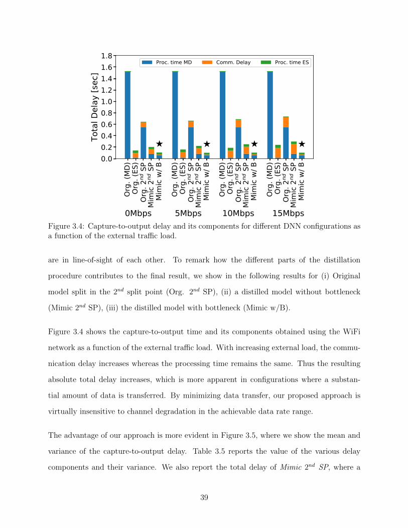
Org. (M

D)Org. (E

S)Org. 2

nd SP

Mimic 2n

d SP

Mimic w/ B

Org. (M

D)Org. (E

S)Org. 2

nd SP

Mimic 2n

d SP

Mimic w/ B

Org. (M

D)Org. (E

S)Org. 2

nd SP

Mimic 2n

d SP

Mimic w/ B

Org. (M

D)Org. (E

S)Org. 2

nd SP

Mimic 2n

d SP

Mimic w/ B

0Mb s 5Mb s 10Mb s 15Mb s

0.00.20.40.60.81.01.21.41.61.8

Total D

elay [sec]

★ ★ ★ ★

Proc. time MD ★omm. Delay Proc. time ES

Figure 3.4: Capture-to-output delay and its components for different DNN configurations asa function of the external traffic load.

are in line-of-sight of each other. To remark how the different parts of the distillation

procedure contributes to the final result, we show in the following results for (i) Original

model split in the 2nd split point (Org. 2nd SP), (ii) a distilled model without bottleneck

(Mimic 2nd SP), (iii) the distilled model with bottleneck (Mimic w/B).

Figure 3.4 shows the capture-to-output time and its components obtained using the WiFi

network as a function of the external traffic load. With increasing external load, the commu-

nication delay increases whereas the processing time remains the same. Thus the resulting

absolute total delay increases, which is more apparent in configurations where a substan-

tial amount of data is transferred. By minimizing data transfer, our proposed approach is

virtually insensitive to channel degradation in the achievable data rate range.

The advantage of our approach is more evident in Figure 3.5, where we show the mean and

variance of the capture-to-output delay. Table 3.5 reports the value of the various delay

components and their variance. We also report the total delay of Mimic 2nd SP, where a

39

0 5 10 15 20 25External Traffic Load [Mbps]

0.1

0.2

0.3

0.4

0.5

0.6

0.7

0.8

Total Delay [sec]

Org. ES proc.Mimic 2nd SPMimic w/ B

Figure 3.5: Average capture-to-output delay over WiFi as a function of the external trafficload.

portion of the DNN model is run at the mobile device. Mimic 2nd SP has a capture-to-output

delay larger than that of Org. ES, as a portion of processing is executed on a slower device

and the amount of data transferred is larger than the actual input. Importantly, the variance

of the proposed Mimic w/B model is smaller compared to that of both Org. ES and Mimic

2nd SP, mostly due to the fact that a smaller amount of traffic transported over the network

reduces protocol interactions such as backoff at the MAC layer and TCP window changes.

This observation is confirmed in Fig. 3.6, which shows time series of capture-to-output delay

in different traffic conditions. The capture-to-output delay offered by the proposed splitting

technique is not only smaller, but is also extremely stable, thus making offloading suitable

to mission critical applications.

We performed an analogous set of experiments using the LTE network. Note that here we

use an UP Board, which is capable of supporting srsLTE. Note that due to the limited

processing speed of the UP Board, which is also executing the data processing task, the

maximum sampling rate, and thus the data rate, is smaller compared to that achievable by

40

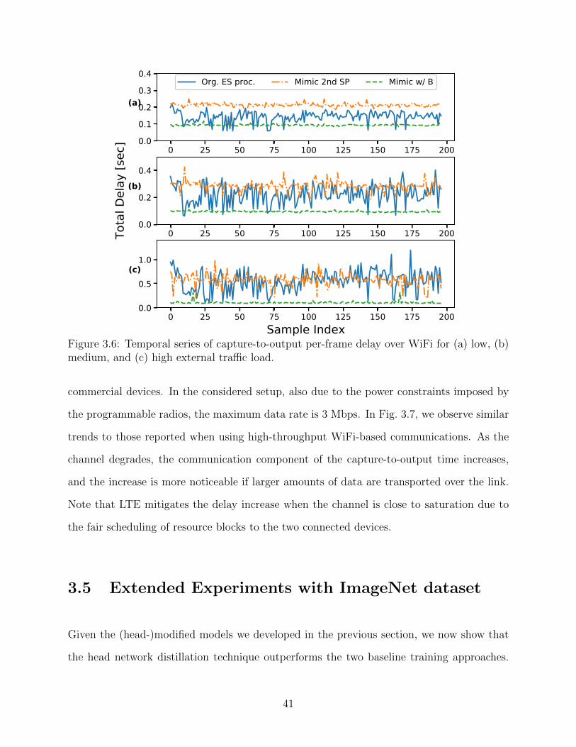
0.0 0.2 0.4 0.6 0.8 1.0Sample Index

0.0

0.2

0.4

0.6

0.8

1.0

Total D

elay [s

ec] 0 25 50 75 100 125 150 175 200

0.00.10.20.30.4

(a)

Org. ES proc. Mimic 2nd SP Mimic w/ B

0 25 50 75 100 125 150 175 2000.0

0.2

0.4(b)

0 25 50 75 100 125 150 175 2000.0

0.5

1.0(c)

Figure 3.6: Temporal series of capture-to-output per-frame delay over WiFi for (a) low, (b)medium, and (c) high external traffic load.

commercial devices. In the considered setup, also due to the power constraints imposed by

the programmable radios, the maximum data rate is 3 Mbps. In Fig. 3.7, we observe similar

trends to those reported when using high-throughput WiFi-based communications. As the

channel degrades, the communication component of the capture-to-output time increases,

and the increase is more noticeable if larger amounts of data are transported over the link.

Note that LTE mitigates the delay increase when the channel is close to saturation due to

the fair scheduling of resource blocks to the two connected devices.

3.5 Extended Experiments with ImageNet dataset

Given the (head-)modified models we developed in the previous section, we now show that

the head network distillation technique outperforms the two baseline training approaches.

41

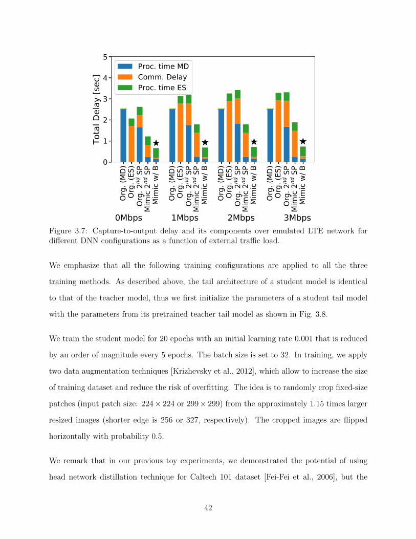
Org.

(MD)

O g.

(ES)

O g.

2nd

SP

Mim

ic 2n

d SP

Mim

ic w/

B

O g.

(MD)

O g.

(ES)

O g.

2nd

SP

Mim

ic 2n

d SP

Mim

ic w/

B

O g.

(MD)

O g.

(ES)

O g.

2nd

SP

Mim

ic 2n

d SP

Mim

ic w/

B

O g.

(MD)

O g.

(ES)

O g.

2nd

SP

Mim

ic 2n

d SP

Mim

ic w/

B

0Mbps 1Mbps 2Mbps 3Mbps

0

1

2

3

4

5

Tota

l Del

ay [s

ec]

★ ★ ★ ★

P oc. time MD★omm. DelayP oc. time ES

Figure 3.7: Capture-to-output delay and its components over emulated LTE network fordifferent DNN configurations as a function of external traffic load.

We emphasize that all the following training configurations are applied to all the three

training methods. As described above, the tail architecture of a student model is identical

to that of the teacher model, thus we first initialize the parameters of a student tail model

with the parameters from its pretrained teacher tail model as shown in Fig. 3.8.

We train the student model for 20 epochs with an initial learning rate 0.001 that is reduced

by an order of magnitude every 5 epochs. The batch size is set to 32. In training, we apply

two data augmentation techniques [Krizhevsky et al., 2012], which allow to increase the size

of training dataset and reduce the risk of overfitting. The idea is to randomly crop fixed-size

patches (input patch size: 224× 224 or 299× 299) from the approximately 1.15 times larger

resized images (shorter edge is 256 or 327, respectively). The cropped images are flipped

horizontally with probability 0.5.

We remark that in our previous toy experiments, we demonstrated the potential of using

head network distillation technique for Caltech 101 dataset [Fei-Fei et al., 2006], but the

42

Figure 3.8: Illustrations of three different training methods. Naive: Naive training, KD:Knowledge Distillation, HND: Head Network Distillation.

models used in this study are specifically designed for a more difficult image classification

task - the ImageNet (ILSVRC 2012) dataset [Russakovsky et al., 2015]. Thus, it is possible

that the teacher models in the previous toy experiments are overparameterized, which could

have enabled small bottlenecks while preserving a comparable accuracy. Herein, we face a

much harder challenge when introducing the bottlenecks. The trained models and code to

reproduce the results are publicly available.1

3.5.1 Training Speed

Given the set of the student models and the training configurations described in the previous

sections, we individually train models using a high-end computer with three GPUs.

Naive training vs. Knowledge distillation First of all, we compare the training per-

formance of naive training and knowledge distillation methods to reproduce the trend in

1https://github.com/yoshitomo-matsubara/head-network-distillation

43

Table 3.6: Validation accuracy* [%] of student models trained with three different trainingmethods.

Method DenseNet-169 DenseNet-201 ResNet-152 Inception-v3

Naive 66.90 (-4.970) 68.92 (-2.950) 72.02 (+0.149) 74.20 (+2.330)

KD 69.37 (-2.500) 70.89 (-0.980) 74.06 (+2.190) 75.46 (+3.589)

HND 72.03 (+0.159) 73.62 (+1.750) 75.13 (+3.259) 75.78 (+3.910)

* ILSVRC 2012 validation dataset (test dataset is not available)** Numbers in brackets indicate differences from MobileNet v2.

the study of Ba and Caruana [2014], which shows that – whole network – student models

trained by knowledge distillation outperform those naively trained on the original dataset.

Figure 3.9a depicts the training time and validation accuracy at the end of each epoch (thus

20 data points) for each pair of student models and training methods. It can be observed how

in the knowledge distillation method the student models achieve higher accuracy compared

to the naive training method used in [Eshratifar et al., 2019b, Hu and Krishnamachari, 2020,

Shao and Zhang, 2020]. This comes at the cost of a longer training time.

Knowledge distillation vs. Head network distillation We showed that knowledge

distillation enables the student models achieve better accuracy compared to naive training.

However, in some cases the models did not reach the accuracy of MobileNetV2 (71.87%), a

small model for mobile devices, and the training process is time-consuming. As illustrated

in Fig. 3.9b, the head network distillation approach consistently helps the student models

not only converge significantly faster, but also achieve even better accuracy compared to the

knowledge distillation method. Recall that we trained exactly the same student models with

the common training configuration described in Section 3.5, but in three different ways as

illustrated in Fig. 3.8. Therefore, we can conclude that these performance improvements are

due to the head network distillation technique we propose.

44

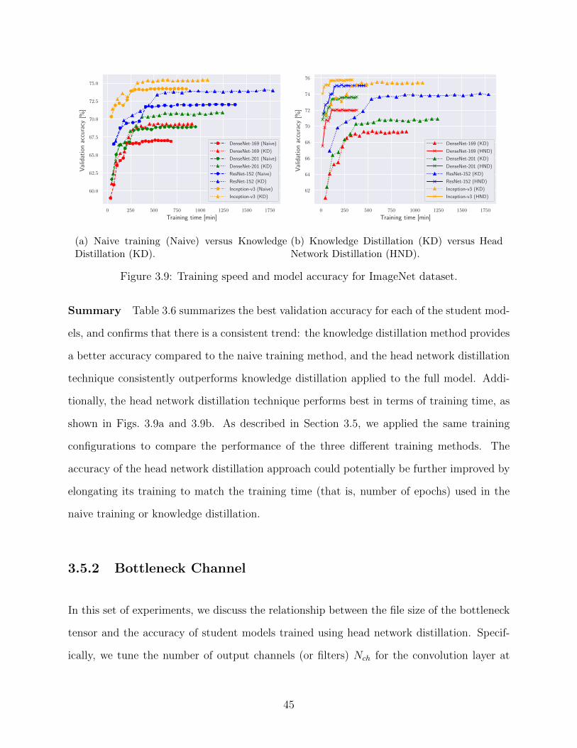
0 250 500 750 1000 1250 1500 1750

Training time [min]

60.0

62.5

65.0

67.5

70.0

72.5

75.0Validationaccuracy

[%]

DenseNet-169 (Naive)

DenseNet-169 (KD)

DenseNet-201 (Naive)

DenseNet-201 (KD)

ResNet-152 (Naive)

ResNet-152 (KD)

Inception-v3 (Naive)

Inception-v3 (KD)

(a) Naive training (Naive) versus KnowledgeDistillation (KD).

0 250 500 750 1000 1250 1500 1750

Training time [min]

62

64

66

68

70

72

74

76

Validationaccuracy

[%]

DenseNet-169 (KD)

DenseNet-169 (HND)

DenseNet-201 (KD)

DenseNet-201 (HND)

ResNet-152 (KD)

ResNet-152 (HND)

Inception-v3 (KD)

Inception-v3 (HND)

(b) Knowledge Distillation (KD) versus HeadNetwork Distillation (HND).

Figure 3.9: Training speed and model accuracy for ImageNet dataset.

Summary Table 3.6 summarizes the best validation accuracy for each of the student mod-

els, and confirms that there is a consistent trend: the knowledge distillation method provides

a better accuracy compared to the naive training method, and the head network distillation

technique consistently outperforms knowledge distillation applied to the full model. Addi-

tionally, the head network distillation technique performs best in terms of training time, as

shown in Figs. 3.9a and 3.9b. As described in Section 3.5, we applied the same training

configurations to compare the performance of the three different training methods. The

accuracy of the head network distillation approach could potentially be further improved by

elongating its training to match the training time (that is, number of epochs) used in the

naive training or knowledge distillation.

3.5.2 Bottleneck Channel

In this set of experiments, we discuss the relationship between the file size of the bottleneck

tensor and the accuracy of student models trained using head network distillation. Specif-

ically, we tune the number of output channels (or filters) Nch for the convolution layer at

45

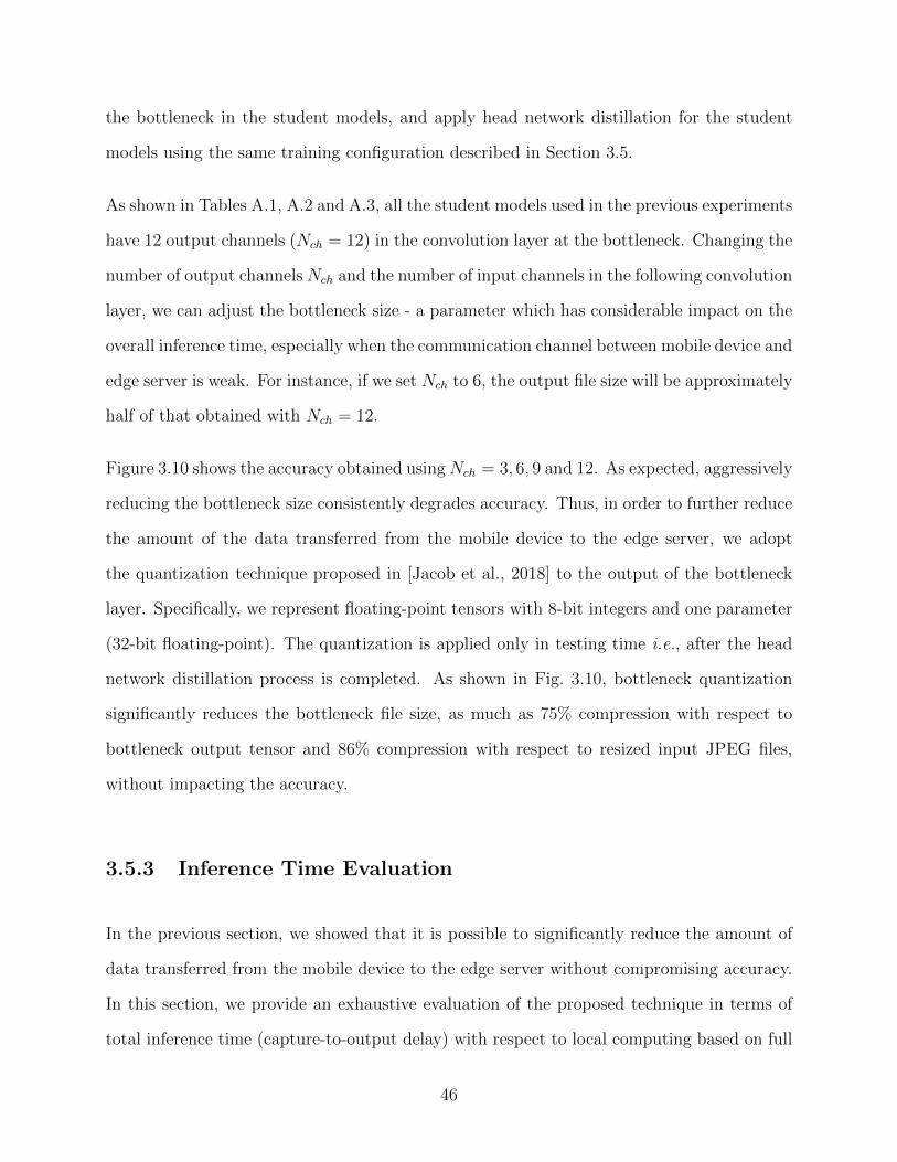
the bottleneck in the student models, and apply head network distillation for the student

models using the same training configuration described in Section 3.5.

As shown in Tables A.1, A.2 and A.3, all the student models used in the previous experiments

have 12 output channels (Nch = 12) in the convolution layer at the bottleneck. Changing the

number of output channelsNch and the number of input channels in the following convolution

layer, we can adjust the bottleneck size - a parameter which has considerable impact on the

overall inference time, especially when the communication channel between mobile device and

edge server is weak. For instance, if we set Nch to 6, the output file size will be approximately

half of that obtained with Nch = 12.

Figure 3.10 shows the accuracy obtained usingNch = 3, 6, 9 and 12. As expected, aggressively

reducing the bottleneck size consistently degrades accuracy. Thus, in order to further reduce

the amount of the data transferred from the mobile device to the edge server, we adopt

the quantization technique proposed in [Jacob et al., 2018] to the output of the bottleneck

layer. Specifically, we represent floating-point tensors with 8-bit integers and one parameter

(32-bit floating-point). The quantization is applied only in testing time i.e., after the head

network distillation process is completed. As shown in Fig. 3.10, bottleneck quantization

significantly reduces the bottleneck file size, as much as 75% compression with respect to

bottleneck output tensor and 86% compression with respect to resized input JPEG files,

without impacting the accuracy.

3.5.3 Inference Time Evaluation

In the previous section, we showed that it is possible to significantly reduce the amount of

data transferred from the mobile device to the edge server without compromising accuracy.

In this section, we provide an exhaustive evaluation of the proposed technique in terms of

total inference time (capture-to-output delay) with respect to local computing based on full

46

10 20 30 40 50 60

Bottleneck file size [KB]

55

60

65

70

75

Validationaccuracy

[%]

DenseNet-169

DenseNet-169 with BQ

DenseNet-201

DenseNet-201 with BQ

ResNet-152

ResNet-152 with BQ

Inception-v3

Inception-v3 with BQ

Figure 3.10: Relationship between bottleneck file size and validation accuracy with/withoutbottleneck quantization (BQ).

models and mobile-specific models (MobileNet v2) and pure edge computing. We note that

naive splitting approaches e.g., Neurosurgeon [Kang et al., 2017] are not used in the following

evaluations as the original benchmark models do not have any small bottleneck point at their

early stage, where their best splitting point would result in either input or output layers.

i.e., pure offloading or local computing. We remark that the focus is to provide solutions

to improve edge computing performance over challenged wireless links, which may present

relatively low or intermittent capacity due to congestion or impaired signal propagation.

Note that we assume a channel where all the transmitted packets are eventually delivered.

This is a common setting in edge computing, and generally in machine learning, frameworks,

and can be realized, for instance, using TCP at the transport layer. Clearly, retransmissions

to resolve packet failures will reduce the perceived data rate, and that shown in the figures

is the resulting effective rate. Herein, as most literature in this area [Kang et al., 2017,

Eshratifar et al., 2019b, Matsubara et al., 2019, Emmons et al., 2019], we also assume that

47

Table 3.7: Hardware specifications.

Computer Processor Freq. RAM

Raspberry Pi 3B+ ARM Cortex A53 (quad-core) 1.2 GHz 1 GB

Jetson TX2

ARM Cortex-A57 (quad-core)+ NVIDIA Denver2 (dual-core)+ 256-core NVIDIA Pascal™ GPU

2.0 GHz 8 GB

Desktop Intel i7-6700K CPU (quad-core)+ NVIDIA GeForce RTX 2080 Ti 4.0 GHz 32 GB

the mobile device is connected to one server at any given time. For instance, the mobile

device could simply use the edge server connected through the best channel.

Table 3.7 summarizes the specifications of the three different computers used as either a

mobile device (MD) or an edge server (ES), and we evaluate the overall inference time in

the three different mobile device-edge server configurations: (i) Raspberry Pi 3B+ – Jetson

TX2, (ii) Raspberry Pi 3B+ – Desktop, and (iii) Jetson TX2 – Desktop.

Gain with respect to Local and Edge Computing

First, we discuss the gain (defined as the ratio of the capture-to-output delay T of a tradi-

tional setting to that provided by our technique) with respect to local and edge computing

with their original (teacher) models, that are defined as TLC/TOurs and TEC/TOurs, respec-

tively. For edge computing, we compute the communication delay based on the JPEG file size

after reshaping sampled input images in the ILSVRC 2012 validation dataset (3× 299× 299

for Inception-v3 and 3× 224× 224 for other models). To compute the communication delay

for our split student models, we use the file size of the quantized tensor at bottleneck, which

are from the last data points (i.e., Nch = 12) with BQ in Fig. 3.10.

Figure 3.11 indicates that splitting the computing load using our student models provides

significant gains compared to locally execution the original (teacher) models on the mobile

48

(a) RPI 3B+ (MD) and JetsonTX2 (ES)

(b) RPI 3B+ (MD) and desktop(ES)

(c) Jetson TX2 (MD) and desk-top (ES)

Figure 3.11: Gains with respect to local computing. MD: mobile device, ES: edge server.

(a) RPI 3B+ (MD) and JetsonTX2 (ES)

(b) RPI 3B+ (MD) and desktop(ES)

(c) Jetson TX2 (MD) and desk-top (ES)

Figure 3.12: Gains with respect to edge computing. MD: mobile device, ES: edge server.

devices unless the channel is extremely weak. As for comparison with edge computing,

the right-side plots of Fig. 3.12 implies that the smaller the difference of computing power

between the mobile device and the edge server the configuration has, the more beneficial the

splitting approach is. From the results, it is also shown that for large enough data rates, then

edge computing is the best option due to the penalty associated with allocated computing

to the weaker device in the system, which overcomes the reduced data transmission time.

Intuitively, such penalty is emphasized in very asymmetric configurations. In less asymmetric

configurations, our technique outperforms edge computing in an extensive range of data rates.

49

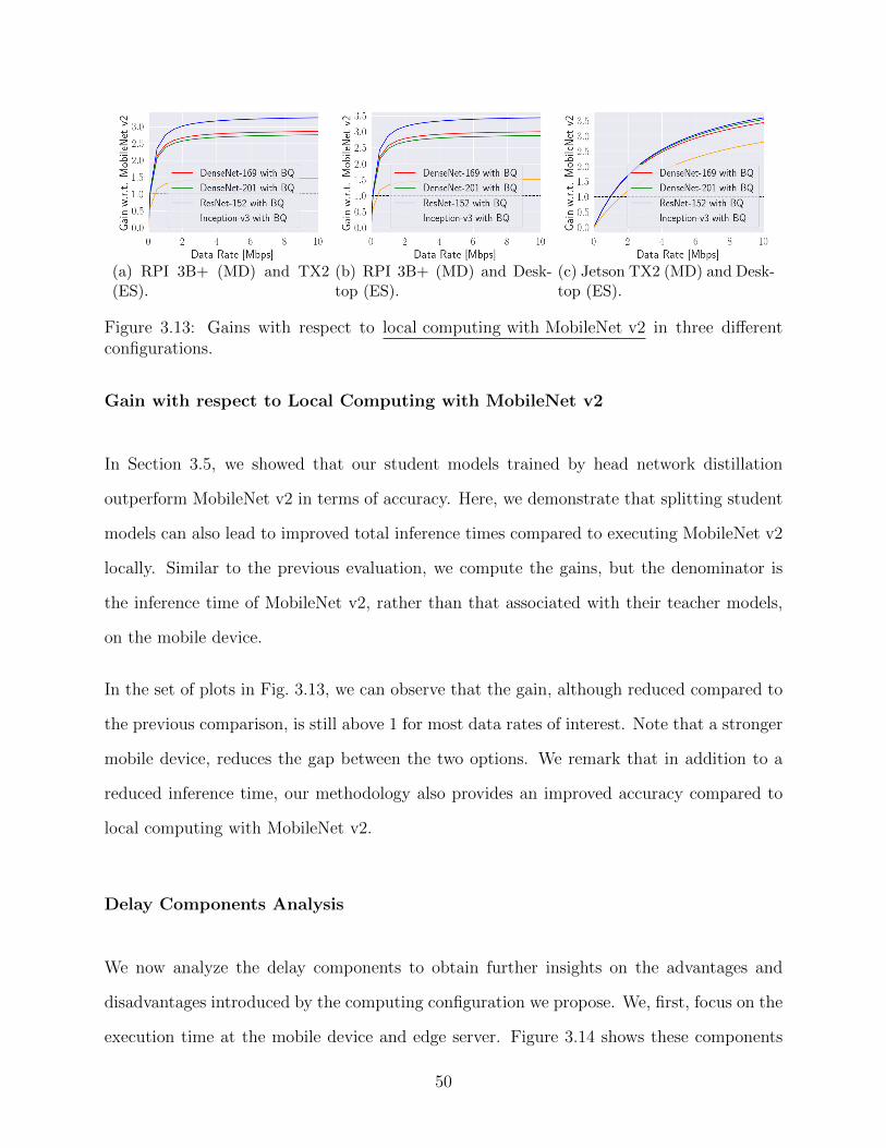
(a) RPI 3B+ (MD) and TX2(ES).

(b) RPI 3B+ (MD) and Desk-top (ES).

(c) Jetson TX2 (MD) and Desk-top (ES).

Figure 3.13: Gains with respect to local computing with MobileNet v2 in three differentconfigurations.

Gain with respect to Local Computing with MobileNet v2

In Section 3.5, we showed that our student models trained by head network distillation

outperform MobileNet v2 in terms of accuracy. Here, we demonstrate that splitting student

models can also lead to improved total inference times compared to executing MobileNet v2

locally. Similar to the previous evaluation, we compute the gains, but the denominator is

the inference time of MobileNet v2, rather than that associated with their teacher models,

on the mobile device.

In the set of plots in Fig. 3.13, we can observe that the gain, although reduced compared to

the previous comparison, is still above 1 for most data rates of interest. Note that a stronger

mobile device, reduces the gap between the two options. We remark that in addition to a

reduced inference time, our methodology also provides an improved accuracy compared to

local computing with MobileNet v2.

Delay Components Analysis

We now analyze the delay components to obtain further insights on the advantages and

disadvantages introduced by the computing configuration we propose. We, first, focus on the

execution time at the mobile device and edge server. Figure 3.14 shows these components

50

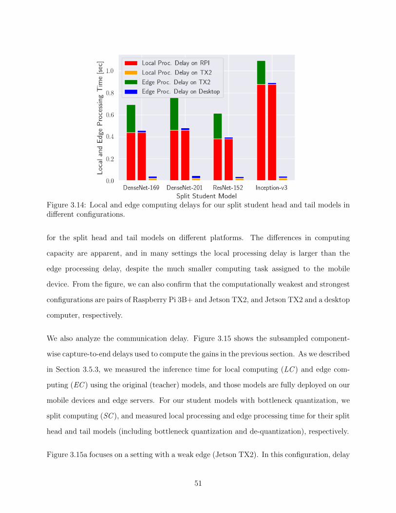
Figure 3.14: Local and edge computing delays for our split student head and tail models indifferent configurations.

for the split head and tail models on different platforms. The differences in computing

capacity are apparent, and in many settings the local processing delay is larger than the

edge processing delay, despite the much smaller computing task assigned to the mobile

device. From the figure, we can also confirm that the computationally weakest and strongest

configurations are pairs of Raspberry Pi 3B+ and Jetson TX2, and Jetson TX2 and a desktop

computer, respectively.

We also analyze the communication delay. Figure 3.15 shows the subsampled component-

wise capture-to-end delays used to compute the gains in the previous section. As we described

in Section 3.5.3, we measured the inference time for local computing (LC ) and edge com-

puting (EC ) using the original (teacher) models, and those models are fully deployed on our

mobile devices and edge servers. For our student models with bottleneck quantization, we

split computing (SC ), and measured local processing and edge processing time for their split

head and tail models (including bottleneck quantization and de-quantization), respectively.

Figure 3.15a focuses on a setting with a weak edge (Jetson TX2). In this configuration, delay

51

LC EC EC EC ECSC SC SC SC

Data rate: 0.1 Mbps 1 Mbps 5 Mbps 10 Mbps

0

2

4

6

8

10Total

InferenceTim

e[sec]

Local Delay

Comm. Delay

Edge Delay

(a) RPI 3B+ (MD) and JetsonTX2 (ES).

LC EC EC EC ECSC SC SC SC

Data rate: 0.1 Mbps 1 Mbps 5 Mbps 10 Mbps

0

2

4

6

8

10

Total

InferenceTim

e[sec]

Local Delay

Comm. Delay

Edge Delay

(b) RPI 3B+ (MD) and Desktop(ES).

LC EC EC EC ECSC SC SC SC

Data rate: 0.1 Mbps 1 Mbps 5 Mbps 10 Mbps

0

1

2

3

4

5

6

Total

InferenceTim

e[sec]

Local Delay

Comm. Delay

Edge Delay

(c) Jetson TX2 (MD) and Desk-top (ES).

Figure 3.15: Capture-to-output delay analysis for teacher and student models of DenseNet-201. LC: Local Computing, EC: Edge Computing, SC: Split Computing.

components associated with processing are – comparably – larger than the communication

delay. Compared to edge computing, the reduced communication delay offered by the head

network distillation technique leads to a smaller capture-to-output delay in impaired channel

conditions. The traditional splitting approach suffers either due to high processing load at

a weaker platform, or higher communication delay due to the need to transport a larger

amount of data to the edge server.

In Fig. 3.15b, a Raspberry Pi 3B+ and high-end desktop computer are used as mobile

device and edge server, respectively. Note that this is the most asymmetric configuration

we can produce with the considered spectrum of hardware. It can be observed that a weak

mobile device strongly penalizes portions of processing executed locally, whereas a limited

channel capacity penalizes the data transfer. The split computing approach we propose

(SC ), by reducing the processing load at the mobile device, and reducing the amount of

data transferred largely outperforms the best alternative – edge computing (ES ) – when the

network capacity is limited. It can be seen how in this configuration the main issue of the

latter option is a large communication delay component, which is only partially offset by

the time needed to execute the split head network at the mobile device. Importantly, both

distillation and quantization are critical to achieve such results, as they allow a considerable

reduction in communication delay. In fact, any other modification of the original model either

52

does not sufficiently reduce the data to be transferred or places an excessive computing load

at the weak mobile device unless a degraded accuracy is tolerated.

3.6 Conclusion

In this chapter, we propose head network distillation in conjunction with bottleneck injection

to improve the performance of edge computing schemes in some parameter regions. We

discussed in detail the structure of the student models we develop to achieve in-network

compression while placing limited amount of computing load to mobile devices and preserve

accuracy. It is demonstrated how bottlenecks with a quantization approach can aggressively

reduce the communication delay when the capacity of the wireless channel between the mobile

device and edge server is limited. We remark that our results are obtained starting from state-

of-the-art models and using Caltech 101 and ImageNet datasets. In this chapter, we put our

focus on image classification tasks and consider resource-constrained edge computing systems

with limited wireless communication capacity where the data rates are limited (≤ 10Mbps).

Further discussions on split computing for different tasks such as object detection are left

for the following chapters.

53

Chapter 4

Towards Detection Tasks

4.1 CNN-based Object Detectors

In this section, we discuss the architecture of recent object detectors based on Convolutional

Neural Network (CNN) that achieve state-of-the-art detection performance. These CNN-

based object detectors are often categorized into either single-stage or two-stage models.

Single-stage models, such as YOLO and SSD series [Redmon et al., 2016, Liu et al., 2016], are

designed to directly predict bounding boxes and classify the contained objects. Conversely,

two-stage models [Ren et al., 2015, He et al., 2017a] generate region proposals as output

of the first stage, and classify the objects in the proposed regions in the second stage. In

general, single-stage models have smaller execution time due to their lower overall complexity

compared to two-stage models, that are superior to single-stage ones in terms of detection

performance.

Recent object detectors, e.g., Mask R-CNN and SSD [He et al., 2017a, Sandler et al., 2018],

adopt state-of-the-art image classification models, such as ResNet [He et al., 2016] and

MobileNet v2 [Sandler et al., 2018], as backbone. The main role of backbones in detection

54

IMG

Layer 0(C,B,R,M)

Layer 1

Layer 2

Layer 3

Layer 4

FPN

RPN

RoI Heads

Coordinates and Classes

Figure 4.1: R-CNN with ResNet-based backbone. Blue modules are from its backbonemodel, and yellow modules are of object detection. C: Convolution, B: Batch normalization,R: ReLU, M: Max pooling layers.

models pretrained on large image datasets, such as the ILSVRC dataset, is feature extraction.

As illustrated in Fig. 4.1, such features include the outputs of multiple intermediate layers in

the backbone. All the features are fed to complex modules specifically designed for detection

tasks, e.g., the feature pyramid network [Lin et al., 2017a], to extract further high-level

semantic feature maps at different scales. Finally, these features are used for bounding box

regression and object class prediction.

In this study, we focus our attention on state-of-the-art two-stage models. Specifically, we

consider Faster R-CNN and Mask R-CNN [Ren et al., 2015, He et al., 2017a] pretrained on

the COCO 2017 datasets. Faster R-CNN is the strong basis of several 1st-place entries [He

et al., 2016] in ILSVRC and COCO 2015 competitions. The model is extended to Mask R-

55

CNN by adding a branch for predicting an object mask in parallel with the existing branch for

bounding box recognition [He et al., 2017a]. Mask R-CNN not only is a strong benchmark,

but also a well-designed framework, as it easily generalizes to other tasks such as instance

segmentation and person keypoint detection. Following the official PyTorch documentation1,

we refer to Mask R-CNN for person keypoint detection as Keypoint R-CNN.

4.2 Challenges and Approaches

We discuss challenges in deploying CNN-based object detectors in three different scenar-

ios: mobile, edge, and split computing. We use total inference time (including the time

needed to transport the data over the wireless channel) and object detection performance as

performance metrics.

4.2.1 Mobile and Edge Computing

In mobile computing the mobile device executes the whole model, and the inference time

is determined by the complexity of the model and local computing power. Due to limita-

tions in the latter, in order to have tolerable inference time, the models must be simple and

lightweight. To this aim, one of the main approaches is to use human-engineered features

instead of those extracted from stacked neural modules. For instance, Mekonnen et al. [2013]

propose an efficient HOG (Histogram Oriented Gradients) based person detection method

for mobile robotics. Designing high-level features of human’s behavior on touch screen, Mat-

subara et al. [2016] propose distance/SVM-based one-class classification approaches to screen

unlocking on smart devices in place of password or fingerprint authentications.

In recent years, however, deep learning methods have been outperforming the models with

1https://pytorch.org/vision/stable/models.html#keypoint-r-cnn

56

human-engineered features in terms of model accuracy. For image classification tasks, Mo-

bileNets [Sandler et al., 2018, Howard et al., 2019] and MNasNets [Tan et al., 2019] are

examples of models designed to be executed on mobile devices, while providing moderate

classification accuracy. Corresponding lightweight object detection models are SSD [Liu

et al., 2016] and SSDLite [Sandler et al., 2018]. Techniques such as model pruning, quanti-

zation and knowledge distillation [Polino et al., 2018, Wei et al., 2018, Hinton et al., 2014]

can be used to produce lightweight models from larger ones.

Table 4.1 summarizes the performance of some models trained on the COCO 2014 minival

dataset as reported in the TensorFlow repository.2 Obviously, the SSD series object detectors

with MobileNet backbones outperform the Faster R-CNN with ResNet-50 backbone in terms

of inference time, but such lightweight models offer degraded detection performance. Note

that in the repository, the COCO 2014 minival split is used for evaluation, and the inference

time is measured on a machine with one NVIDIA GeForce GTX TITAN X, which is clearly

not suitable to be embedded in a mobile device. Also, the values reported in Table 4.1 are

given for models implemented with the TensorFlow framework with input images resized to

600 × 600, though some of the models in the original work such as Faster R-CNN [Ren et al.,

2015] use different resolutions. In general, the classification/detection performance is often

compromised in mobile computing due to their limited computing power.

Table 4.2 highlights that it would be impractical to deploy some of the powerful object

detectors on weak devices. Specifically, on Raspberry Pi 4, R-CNN object detectors with

even the smallest backbone in the family took 20–30 seconds for prediction per a resized

image of which shorter side resolution is 800 pixels, following [Ren et al., 2015, He et al.,

2017a]. For both Faster and Mask R-CNNs, the execution time on NVIDIA Jetson TX2 and

a desktop machine with an NVIDIA RTX 2080 Ti is sufficiently small to support real-time

applications .

2https://github.com/tensorflow/models/blob/master/research/object_detection/g3doc/tf1_

detection_zoo.md#coco-trained-models

57

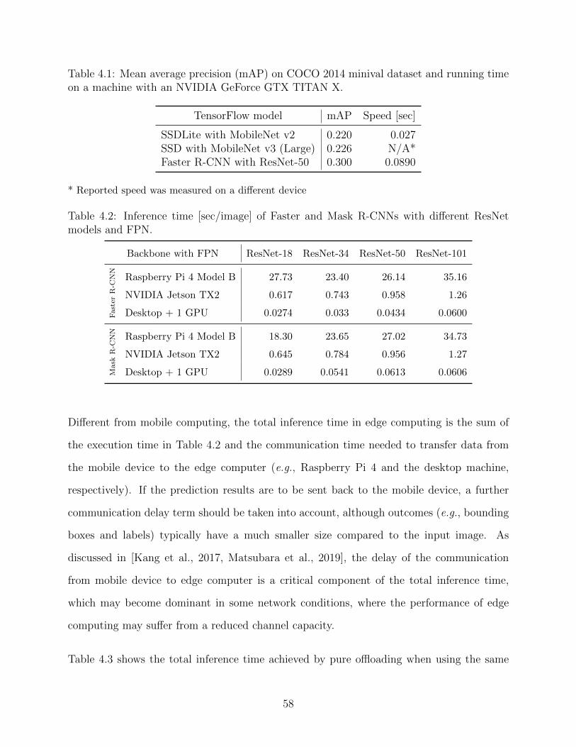
Table 4.1: Mean average precision (mAP) on COCO 2014 minival dataset and running timeon a machine with an NVIDIA GeForce GTX TITAN X.

TensorFlow model mAP Speed [sec]

SSDLite with MobileNet v2 0.220 0.027SSD with MobileNet v3 (Large) 0.226 N/A*Faster R-CNN with ResNet-50 0.300 0.0890

* Reported speed was measured on a different device

Table 4.2: Inference time [sec/image] of Faster and Mask R-CNNs with different ResNetmodels and FPN.

Backbone with FPN ResNet-18 ResNet-34 ResNet-50 ResNet-101

Faster

R-C

NN

Raspberry Pi 4 Model B 27.73 23.40 26.14 35.16

NVIDIA Jetson TX2 0.617 0.743 0.958 1.26

Desktop + 1 GPU 0.0274 0.033 0.0434 0.0600

Mask

R-C

NN

Raspberry Pi 4 Model B 18.30 23.65 27.02 34.73

NVIDIA Jetson TX2 0.645 0.784 0.956 1.27

Desktop + 1 GPU 0.0289 0.0541 0.0613 0.0606

Different from mobile computing, the total inference time in edge computing is the sum of

the execution time in Table 4.2 and the communication time needed to transfer data from

the mobile device to the edge computer (e.g., Raspberry Pi 4 and the desktop machine,

respectively). If the prediction results are to be sent back to the mobile device, a further

communication delay term should be taken into account, although outcomes (e.g., bounding

boxes and labels) typically have a much smaller size compared to the input image. As

discussed in [Kang et al., 2017, Matsubara et al., 2019], the delay of the communication

from mobile device to edge computer is a critical component of the total inference time,

which may become dominant in some network conditions, where the performance of edge

computing may suffer from a reduced channel capacity.

Table 4.3 shows the total inference time achieved by pure offloading when using the same

58

Table 4.3: Pure offloading time [sec] (data rate: 5Mbps) of detection models with differentResNet backbones on a high-end edge server with an NVIDIA GeForce RTX 2080 Ti.

Model \Backbone with FPN ResNet-18 ResNet-34 ResNet-50 ResNet-101

Faster R-CNN 0.456 0.462 0.472 0.489Mask R-CNN 0.458 0.4832 0.4904 0.4897Keypoint R-CNN 0.469 0.473 0.481 0.498

models. In these results, the execution time is computed using a high-end desktop computer

with Intel Core i7-6700K CPU (4.00GHz), 32GB RAM, and a NVIDIA GeForce RTX 2080

Ti as edge server, and the channel provides the relatively low, data rate of 5Mbps to the

image stream. It can be seen that in this setting, how reducing the model size by distilling

the whole detector [Li et al., 2017b, Chen et al., 2017a, Wang et al., 2019] does not lead to

substantial total delay savings, while offloading is generally advantageous compared to local

computing.

4.2.2 Split Computing

Split computing is an intermediate option between mobile and edge computing. The core

idea is to split models into head and tail portions, which are deployed at the mobile device

and edge computer, respectively. To the best of our knowledge, Kang et al. [2017] were the

first to propose to split deep neural network models. However, the study simply proposed

to optimize where to split the model, leaving the architecture unaltered.

In split computing, the total inference time is sum of three components: mobile processing

time, communication delay, and edge processing time. To shorten the inference time in

split computing compared to those of mobile and edge computing, the core challenge is to

significantly reduce communication delay while leaving a small portion of computational load

on mobile device for compressing the data to be transferred to edge server. Splitting models

59

in a straightforward way, as suggested in [Kang et al., 2017], however, does not lead to an

improvement in performance in most cases. The tension is between the penalty incurred by

assigning a portion of the overall model to a weaker device (compared to the edge computer)

and the potential benefit of transmitting a smaller amount of data. However, most models

do not present “natural” bottlenecks in their design, that is, layers with a small number

of output nodes, corresponding to a small tensor to be propagated to the edge computer.

In fact, the neurosurgeon framework locates pure mobile or edge computing as the optimal

computing strategies in most models.

Building on the work of Kang et al. [2017], recent contributions propose DNN splitting meth-

ods [Teerapittayanon et al., 2017, Li et al., 2018a, Eshratifar et al., 2019b, Matsubara et al.,

2019, Emmons et al., 2019, Hu and Krishnamachari, 2020, Shao and Zhang, 2020]. Most of

these studies, however, (1) do not evaluate models using their proposed lossy compression

techniques [Emmons et al., 2019], (2) lack of motivation to split the models as the size of the

input data is exceedingly small, e.g., 32 × 32 pixels RGB images in [Teerapittayanon et al.,

2017, Hu and Krishnamachari, 2020, Shao and Zhang, 2020], (3) specifically select models

and network conditions in which their proposed method is advantageous [Li et al., 2018a],

and/or (4) assess proposed models in simple classification tasks such as miniImageNet, Cal-

tech 101, CIFAR-10, and -100 datasets [Eshratifar et al., 2019b, Matsubara et al., 2019, Hu

and Krishnamachari, 2020, Shao and Zhang, 2020].

Similar to CNN-based image classification models, it is not possible to reduce the inference

time of CNN-based object detectors by naive splitting methods without altering the models’

architecture. This is due to the designs of the early layers of the models, which amplify

the input data size. It would be worth noting that Matsubara et al. [2019] apply a loseless

compression technique, a standard Zip compression, to intermediate outputs of all the split-

table layers in a CNN model, and show the compression gain is not sufficient to significantly

reduce inference time in split computing.

60

Figure 4.2: Layer-wise output tensor sizes of Faster and Mask R-CNNs scaled by input tensorsize (3× 800× 800).

Figure 4.2 illustrates this effect by showing the amplification of the data at each of core

layers in Faster and Mask R-CNNs with ResNet-50, compared to the input tensor size (3×

800× 800). Note that these models are designed for images whose shorter side resolution is

800 pixels [Ren et al., 2015, He et al., 2017a]. The trends confirm that there is no splitting

point (below blue line) in any of the early layers. Therefore, naive splitting does not result

in any gain in terms of communication delay. We note that different from the Faster R-CNN

model, the output tensor of the RoI Heads in the Mask R-CNN model is significantly larger

than the input tensor. As the model emits not only bounding boxes and object classes, but

also pixel-level masks for segmentation, the last tensor size surges in Fig. 4.2 (green dotted

line), but the general trend looks the same with Faster R-CNN model when using bounding

boxes and object classes only.

A promising, but challenging, solution to reduce the inference time in challenged networks

is to introduce a small bottleneck within the model, and split the model at that layer [Mat-

61

subara et al., 2019]. In the following section, we discuss bottleneck injection for CNN-based

object detectors, specifically Faster and Mask R-CNNs, and present preliminary experimen-

tal results supporting this strategy.

4.3 In-Network Neural Compression

4.3.1 Background

As discussed earlier, the weak point of pure edge computing is the communication delay:

when the capacity of the channel interconnecting the mobile device and edge server is de-

graded by a poor propagation environment, mobility, interference and/or traffic load, trans-

ferring the model input to the edge server may result in a large overall capture-to-output

delay T . Thus, in challenged channel conditions, making edge computing effective necessi-

tates strategies to reduce the amount of data to be transported over the channel.

The approach we take herein is to modify the structure of the model to obtain in-network

compression and improve the efficiency of network splitting. We remind that in network

splitting, the output of the last layer of the head model is transferred to the edge, instead

of the model input. Compression, then, corresponds to splitting the model at layers with a

small number of nodes which generate small outputs to be transmitted over the channel. In

our approach, the splitting point coincides with the layer where compression is achieved.

Unfortunately, layers with a small number of nodes appear only in advanced portions of

object detectors, while early layers amplify the input to extract features. However, splitting

at late layers would position most of the computational complexity at the weaker mobile

device. This issue was recently discussed in [Matsubara et al., 2019, Matsubara and Levorato,

2020] for image classification and object detection models, reinforcing the results obtained

62

in [Kang et al., 2017] on traditional network splitting.

In [Matsubara et al., 2019], we proposed to introduce bottleneck layers, that is, layers with a

small number of nodes, in the early stages of image classification models. To reduce accuracy

loss as well as computational load at the mobile device, the whole head section of the model

is reduced using distillation. The resulting small model contains a bottleneck layer followed

by a few layers that translate the bottleneck layer’s output to the output of the original head

model. Note that the layers following the bottleneck layers are then attached to the original

tail model and executed at the edge server.

The distillation process attempts to make the output of the new head model as close as

possible to the original head. At an intuitive level, when introducing bottleneck layers

this approach is roughly equivalent to train a small asymmetric encoder-decoder pipeline

whose boundary layer produces a compressed version of the input image used by the decoder

to reconstruct the output of the head section, rather than the image. Interestingly, it is

shown that the distillation approach can achieve high compression rates while preserving

classification performance even is complex classification tasks.

This paper builds on this approach [Matsubara et al., 2019, Matsubara and Levorato, 2020]

to obtain in-network compression with further improved detection performance in object

detection tasks. Specifically, we generalize the head network distillation (HND) technique,

and apply it to the state of the art detection models described in the previous section (Faster

R-CNN, Mask R-CNN, and Keypoint R-CNN).

The key challenge originates from the structural differences between the models for these two

classes of vision tasks. As discussed in the previous section, although image classification

models are used as backbones of detection models, there is a trend of using outputs of

multiple intermediate layers as features fed to modules designed for detection such as the

FPN (Feature Pyramid Network) [Lin et al., 2017a]. This makes the distillation of head

63

models difficult, as they would need to embed multiple bottleneck layers at the points in

the head network whose output is forwarded to the detectors. Clearly, the amount of data

transmitted over the network would be inevitably larger as multiple outputs would need to

be transferred. Additionally, we empirically show that injecting smaller bottlenecks resulted

in degraded detection performance [Matsubara and Levorato, 2020].

To overcome this issue, we redefine here the head distillation technique to (i) introduce the

bottleneck at the very early layers of the network, and (ii) refine the loss function used to

distill the mimicking head model to account for the loss induced on forwarded intermediate

layers’ outputs. We remark that in network distillation (see Fig. 4.4) applied to head-tail

split models, the head portion of the model (red) is distilled introducing a bottleneck layer,

and the original teacher’s architecture and parameters for the tail section (green) are reused

without modification. We note that this allows fast training, as only a small portion of the

whole model is retrained.

4.3.2 R-CNN Model Analysis

One of the core challenges in introducing bottlenecks to R-CNN object detectors is that

the bottleneck needs to be introduced in earlier stages of the detector compared to image

classification models. As illustrated in Fig. 4.1, the first branch of the network is after Layer

1. As a result, the bottleneck needs to be injected before the layer to avoid the need to

forward multiple tensors produced by the branches (Figs. 4.1 and 4.2).

The amount of computational load assigned to the mobile device should be considered as

well when determining the bottleneck placement. In fact, the execution time of the head

model, which will be deployed on the mobile device, is a critical component to minimize the

total inference time. Figures 4.3a and 4.3b depict the number of parameters of each model

used for partial inference on the mobile device when splitting the model at specific modules.

64

(a) Faster R-CNN (b) Mask R-CNN

Figure 4.3: Cumulative number of parameters in R-CNN object detection models.

The reported values provide a rough estimate of the head model’s complexity as a function

of the splitting point.

Recall that feature pyramid network (FPN), region proposal network (RPN), and region

of interest (RoI) Heads in the R-CNN models are designed specifically for object detection

tasks, and all the modules before them are originally from an image classification model

(ResNet models [He et al., 2016] in this study). Because of not only the models’ branching,

but the trends in these figures, it is clear that the bottleneck, and thus the splitting point,

should be placed before “Layer 1”.

4.3.3 Bottleneck Positioning and Head Structure

As discussed in Section 4.3.2, the output of early blocks of the backbone are forwarded to the

detectors. In order to avoid the need to introduce the bottlenecks in multiple sections and

transmit their output, the bottleneck should be introduced before “Layer 1” (L1) module of

the model, whose output is the first to be forwarded to FPN.

65

FPNBackboneRPN RoI

Heads

Class(es) and

Bounding Box(es)

FPNBackboneRPN RoI

Heads

Class(es) and

Bounding Box(es)

SSE LossesImage

Teacher

Student

Figure 4.4: Generalized head network distillation for R-CNN object detectors. Green mod-ules correspond to frozen blocks of individual layers of/from the teacher model, and redmodules correspond to blocks we design and train for the student model. L0-4 indicatehigh-level layers in the backbone. In this study, only backbone modules (orange) are usedfor training.

Furthermore, Matsubara et al. [2019] attempted to introduce a bottleneck in the first convo-

lution layer of DenseNet-169 [Huang et al., 2017]. The bottleneck uses 4 output channels in

place of 64 channels, so that the output tensor of the layer is smaller than the input tensor

to the model. Using Caltech 101 dataset, they naively trained the redesigned model, that

significantly degraded classification accuracy even despite the relative low complexity of the

dataset compared to the ILSVRC dataset.

Based on the analysis and results, we attempt to introduce a bottleneck to “Layer 1”, that

consists of multiple low-level modules such as convolution layers. Here, we redesign the layer

1 by pruning a couple of layers and adjust hyperparameters to make its output shape match

that of the layer 1 in the original model. The redesigned layer 1 has a small bottleneck with

C output channels, a key parameter to control the balance between detection performance

and bottleneck size.

Compared to the framework developed in [Matsubara et al., 2019], this has two main im-

plications. Firstly, the aggregate complexity of the head model is fairly small, and we do

not need to significantly reduce its size to minimize computing load at the mobile device.

Secondly, in these first layers the extracted features are not yet well defined, and devising

an effective structure for the bottleneck is challenging.

66

Figure 4.4 summarizes the architecture. The difference between the overall teacher and

student models are the high-level layers 0 and 1 (L0 and L1), while the rest of the architecture

and their parameters is left unaltered. The architecture of L0 in the student models is

also identical to that in the teacher models, but their parameters are retrained during the

distillation process. The L1 in student models is designed to have the same output shape as

the L1 in teacher models, while we introduce a bottleneck layer within the module.

The architectures of layer 1 in teacher and student models are summarized in our supplemen-

tary material. The architecture will be used in all the considered object detection models:

Faster, Mask, and Keypoint R-CNNs. Our introduced bottleneck point is designed to output

a tensor whose size is approximately 6− 7% of the input one. Specifically, we introduce the

bottleneck point by using an aggressively small number of output channels in the convolution

layer and amplifying the output with the following layers. As we design the student’s layers,

tuning the number of channels in the convolution layer is a key for our bottleneck injection.

The main reason we consider the number of channels as a key hyperparameter is that differ-

ent from CNNs for image classification, the input and output tensor shapes of the detection

models, including their intermediate layers, are not fixed [Ren et al., 2015, He et al., 2017a,

Paszke et al., 2019]. Thus, it would be difficult to have the output shapes of student model

match those of teacher model, that must be met for computing loss values in distillation pro-

cess described later. For such models, other hyperparameters such as kernel size k, padding p,

and stride s cannot be changed aggressively while keeping comparable detection performance

since they change the output patch size in each channel, and some input elements may be

ignored depending on their hyperparameter values. The detail of the network architectures

is provided in Appendix B.

67

4.3.4 Loss Function

In head network distillation (HND) initially applied to image classification [Matsubara et al.,

2019], the loss function used to train the student model is defined as Eq. (3.1), which is

LHND(x) = ∥fShead(x)− fThead(x)∥2,

where fShead and fThead are sequences of the first LShead and LT

head layers in student and teacher

models, respectively. The loss function, thus, is simply the sum of squared errors (SSE)

between the outputs of last student and teacher layers, and the student model is trained to

minimize the loss. This simple approach produced good results in image classification tasks.

Due to the convoluted structure of object detection models, the design of the loss function

needs to be revisited in order to build effective head models. As described earlier, the output

of multiple intermediate layers in the backbone are used as features to detect objects. As a

consequence, the “mimicking loss” at the end of L1 in the student model will be inevitably

propagated as tensors are fed forward, and the accumulated loss may degrade the overall

detection performance for compressed data size [Matsubara and Levorato, 2020].

For this reason, we reformulate the loss function as follows:

LGHND(x) =∑j∈J

λj · Lj(fSj(x), fTj (x

)), (4.1)

where j is loss index, λj is a scale factor (hyperparameter) associated with loss Lj, and fTj and

fSj indicate the corresponding subset of teacher and student models (functions of input data

x) respectively. The total loss, then, is the sum of |J | weighted losses. Following Eq. (4.1),

the previously proposed head network distillation technique [Matsubara et al., 2019] can be

seen as a special case of our proposed technique.

68

Figure 4.5: Normalized bottleneck tensor size vs. mean average precision of Faster and MaskR-CNNs with FPN.

4.3.5 Detection Performance Evaluation

As we modify the structure and parameters of state-of-the-art models to achieve an effective

splitting, we need to evaluate the resulting object detection performance. In the following

experiments, we use the same distillation configurations for both the original and our gen-

eralized head network distillation techniques. Distillations are performed using the COCO

2017 training datasets and the following hyperparameters. Student models are trained for

20 epochs, and batch size is 4. The models’ parameters are optimized using Adam [Kingma

and Ba, 2015] with an initial learning rate of 10−3, which is decreased by a factor 0.1 at

the 5th and 15th epochs for Faster and Mask R-CNNs. The number of training samples in

the person keypoint dataset is smaller than that in object detection dataset, thus we train

Keypoint R-CNN student models for 35 epochs and decrease the learning rate by a factor of

0.1 at the 9th and 27th epochs.

69

Table 4.4: Performance of pretrained and head-distilled (3ch) models on COCO 2017 vali-dation datasets* for different tasks.

R-CNN with FPN Faster R-CNN Mask R-CNN Keypoint R-CNNApproach \ Metrics BBox BBox Mask BBox Keypoints

Pretrained (Teacher) † 0.370 0.379 0.346 0.546 0.650

HND 0.339 0.350 0.319 0.488 0.579Ours 0.358 0.370 0.337 0.532 0.634Ours + BQ (16 bits) 0.358 0.370 0.336 0.532 0.634Ours + BQ (8 bits) 0.355 0.369 0.336 0.530 0.628

* Test datasets for these detection tasks are not publicly available.† https://github.com/pytorch/vision/releases/tag/v0.3.0

When using the original head network distillation proposed in [Matsubara et al., 2019], the

sum of squared error loss is minimized (Eq. (3.1)) using the outputs of the high-level layer 1

(L1) of the teacher and student models. In the head network distillation for object detection

we propose, we minimize the sum of squared error losses in Eq. (4.1) using the output of

the high-level layers 1–4 (L1–4) with scale factors λ∗ = 1. Note that in both the cases,

we update only the parameters of the layers 0 and 1, and those of the layers 2, 3 and 4 are

fixed. Quite interestingly, the detection performance degraded when we attempted to update

the parameters of layers 1 to 4 in our preliminary experiments. As performance metric,

we use mAP (mean average precision) that is averaged over IoU (Intersection-over-Union)

thresholds in object detection boxes (BBox), instance segmentation (Mask) and keypoint

detection tasks.

Figure 4.5 reports the detection performance of teacher models, and models with differ-

ent bottleneck sizes trained by the original and our generalized head network distillation

techniques. For the bottleneck-injected Faster and Mask R-CNNs, the use of our proposed

loss function significantly improves mAP compared to models distilled using the original

head network distillation (HND) [Matsubara and Levorato, 2020]. Due to limited space, we

show the detection performance of Keypoint R-CNN with an injected bottleneck (3ch) in

Table 4.4. Clearly, the introduction of the bottleneck, and corresponding compression of the

70

output of that section of the network, induces some performance degradation with respect

to the original teacher model.

4.3.6 Qualitative Analysis

Figure 4.6 shows sampled input and output images from Mask and Keypoint R-CNNs.

Comparing to the outputs of the original models (Figs. 4.6e - 4.6h), our Mask and Keypoint

R-CNN detectors distilled by the original head network distillation (HND) [Matsubara et al.,

2019] suffer from false positives and negatives shown in Figs. 4.6i - 4.6k. As for those distilled

by our generalized head network distillation, their detection performance look qualitatively

comparable to the original models. In our examples, the only significant difference between

outputs of the original models and ours is that a small cell phone hold by a white-shirt man

that is not detected by our Mask R-CNN shown in Fig. 4.6m.

4.3.7 Bottleneck Quantization (BQ)

Using our generalized head network distillation technique, we introduce small bottlenecks

within the student R-CNN models. Remarkably, the bottlenecks save up to approximately

94% of tensor size to be offloaded, compared to input tensor. However, compared to the input

JPEG, rather than its tensor representation [Matsubara and Levorato, 2020], the compression

gain is still not satisfactory (see Table 4.5). To achieve more aggressive compression gains,

we quantize the bottleneck output. Quantization techniques for deep learning [Li et al.,

2018a, Jacob et al., 2018] have been recently proposed to compress models, reducing the

amount of memory used to store them. Here, we instead use quantization to compress the

bottleneck output specifically, by representing 32-bit floating-point tensors with 16- or 8-bit.

We can simply cast bottleneck tensors (32-bit by default) to 16-bit, but the data size ratio

71

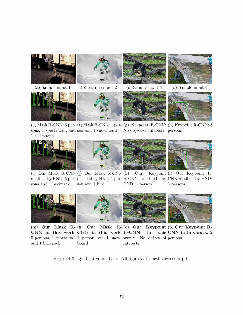
(a) Sample input 1 (b) Sample input 2 (c) Sample input 3 (d) Sample input 4

(e) Mask R-CNN: 5 per-sons, 1 sports ball, and1 cell phone

(f) Mask R-CNN: 1 per-son and 1 snowboard

(g) Keypoint R-CNN:No object of interests

(h) Keypoint R-CNN: 3persons

(i) Our Mask R-CNNdistilled by HND: 5 per-sons and 1 backpack

(j) Our Mask R-CNNdistilled by HND: 1 per-son and 1 bird

(k) Our KeypointR-CNN distilled byHND: 1 person

(l) Our Keypoint R-CNN distilled by HND:3 persons

(m) Our Mask R-CNN in this work:5 persons, 1 sports balland 1 backpack

(n) Our Mask R-CNN in this work:1 person and 1 snow-board

(o) Our KeypointR-CNN in thiswork: No object ofinterests

(p) Our Keypoint R-CNN in this work: 2persons

Figure 4.6: Qualitative analysis. All figures are best viewed in pdf.

72

Table 4.5: Ratios of bottleneck (3ch) data size and tensor shape produced by head portionto input data.

Input Bottleneck Quantized Bottleneck(JPEG) 32 bits 16 bits 8 bits

Data size 1.00 2.56 1.28 0.643Tensor shape 1.00 0.0657 0.0657 0.0657

is still above 1 in Table 4.5, that means there would be no gain of inference time as it take

longer to deliver the data to the edge server compared to pure offloading. Thus, we apply the

quantization technique [Jacob et al., 2018] to represent tensors with 8-bit integers and one

32-bit floating-point value. Note that quantization is applied after distillation to simplify

training. Inevitably, quantization will result in some information loss, which may affect the

detection performance of the distilled models. Quite interestingly, our results indicate that

there is no significant detection performance loss for most of the configurations in Table 4.4,

while achieving a considerable reduction in terms of data size as shown in Table 4.5. In

Section 4.5 we report results using 8-bit quantization.

4.4 Neural Image Prefiltering

In this section, we exploit a semantic difference between image classification and object

detection tasks to reduce resource usage. While every image is used for inference, only a

subset of images produced by the mobile device contain objects within the overall set of

detected classes. Intuitively, the execution of the object detection module is useful only if at

least one object of interest appear in the vision range. Figures 4.8c and 4.8d are examples of

pictures without objects of interest for Keypoint R-CNN, as this model is trained to detect

people and simultaneously locate their keypoints. We attempt then, to filter out the empty

images before they are transmitted over the channel and processed by the edge server.

73

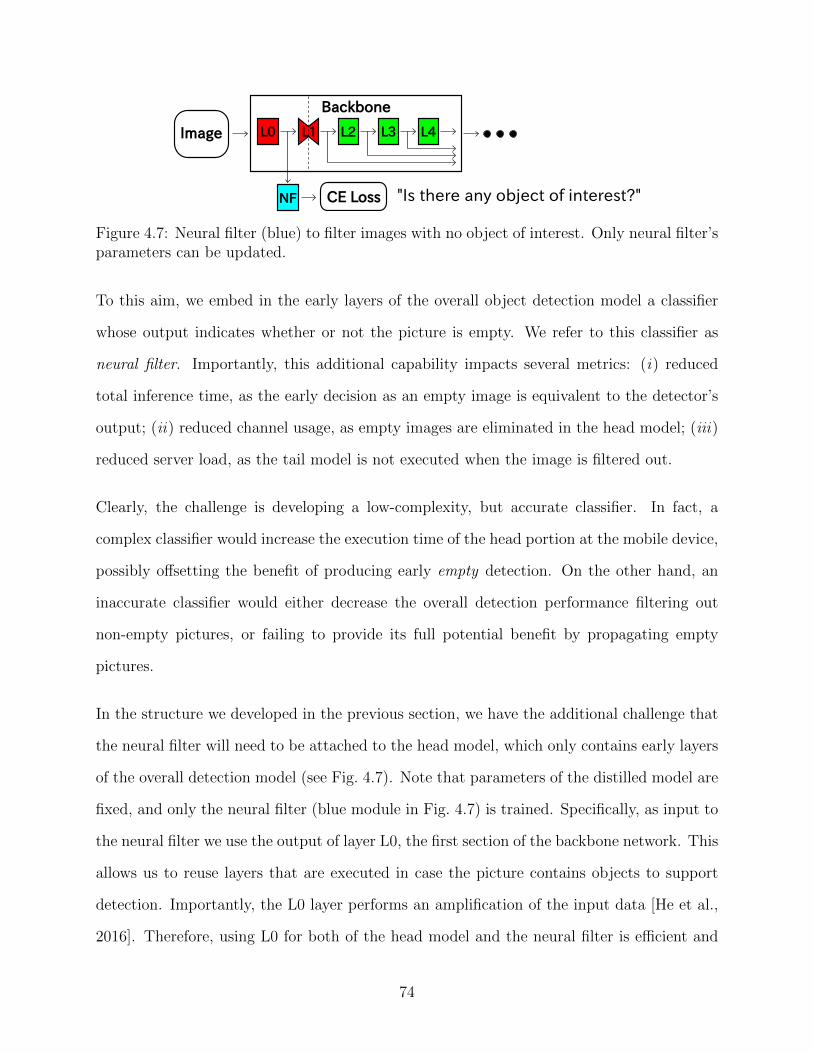
Backbone

L0 L2 L3 L4

NF

L1

CE Loss

Image

"Is there any object of interest?"

Figure 4.7: Neural filter (blue) to filter images with no object of interest. Only neural filter’sparameters can be updated.

To this aim, we embed in the early layers of the overall object detection model a classifier

whose output indicates whether or not the picture is empty. We refer to this classifier as

neural filter. Importantly, this additional capability impacts several metrics: (i) reduced

total inference time, as the early decision as an empty image is equivalent to the detector’s

output; (ii) reduced channel usage, as empty images are eliminated in the head model; (iii)

reduced server load, as the tail model is not executed when the image is filtered out.

Clearly, the challenge is developing a low-complexity, but accurate classifier. In fact, a

complex classifier would increase the execution time of the head portion at the mobile device,

possibly offsetting the benefit of producing early empty detection. On the other hand, an

inaccurate classifier would either decrease the overall detection performance filtering out

non-empty pictures, or failing to provide its full potential benefit by propagating empty

pictures.

In the structure we developed in the previous section, we have the additional challenge that

the neural filter will need to be attached to the head model, which only contains early layers

of the overall detection model (see Fig. 4.7). Note that parameters of the distilled model are

fixed, and only the neural filter (blue module in Fig. 4.7) is trained. Specifically, as input to

the neural filter we use the output of layer L0, the first section of the backbone network. This

allows us to reuse layers that are executed in case the picture contains objects to support

detection. Importantly, the L0 layer performs an amplification of the input data [He et al.,

2016]. Therefore, using L0 for both of the head model and the neural filter is efficient and

74

(a) 2 persons (b) 1 person (c) No person (d) No person

Figure 4.8: Sample images in COCO 2017 training dataset.

effective.

In this study, we introduce a neural filter to a distilled Keypoint R-CNN model as illustrated

in Fig. 4.7. We describe the architecture of the neural filter in Appendix B. Approximately

46% of images in the COCO 2017 person keypoint dataset have no object of interest, and

Figures 4.8c and 4.8d are sample images we would like to filter out. The design of the neural

filter is reported in our supplementary material, and we train the model for 30 epochs. Each

image is labeled as “positive” if it contains at least one valid object, and as “negative“

otherwise. We use cross entropy loss to optimize model’s parameters by SGD with an initial

learning rate 10−3, momentum 0.9, weight decay 10−4, and batch size of 2. The learning rate

is decreased by a factor of 0.1 at the 15th and 25th epochs. Our neural filter achieved 0.919

ROC-AUC on the validation dataset.

The output values of the neural filter are softmaxed i.e., [0, 1]. In order to preserve the

performance of the distilled Keypoint R-CNN model when using the neural filter, we set

a small threshold for prefiltering to obtain a high recall, while images without objects of

interest are prefiltered only when the neural filter is negatively confident. Specifically, we

filter out images with prediction score smaller than 0.1. The BBox and Keypoint mAPs of

distilled Keypoint R-CNN with BQ (8-bit) and neural filter are 0.513 and 0.619 respectively.

As shown in the next section, the detection performance slightly degraded by the neural

filter results in a perceivable reduction of the total inference time in the considered datasets.

75

4.5 Latency Evaluation

In this section, we evaluate the total inference time T of capture-to-output pipelines. We

use the NVIDIA Jetson TX2 as mobile device and the high-end desktop computer with

a NVIDIA GeForce RTX 2080 Ti as edge server. Clearly, scenarios with weaker mobile

devices and edge servers will see a reduced relative weight of the communication component

of the total delay, thus possibly advantaging our technique compared to pure offloading. On

the other hand, a strongly asymmetric system, where the mobile device has a considerably

smaller computing capacity compared to the edge server will penalize the execution of even

small computing tasks at the mobile device, as prescribed by our approach.

We compare three different configurations: local computing, pure offloading, and split com-

puting using network distillation. Here, we do not consider naive splitting approaches such

as Neurosurgeon [Kang et al., 2017] as the original R-CNN models used in this study do

not have any small bottleneck point [Matsubara and Levorato, 2020], and the best splitting

point would result in either input or output layers i.e., pure offloading or local computing.

However, we consider the same data rates for vision task as in [Kang et al., 2017], and focus

thus on rates below 10Mbps. Note that all the R-CNN models are designed to have an

input image whose shorter side has 800 pixels. In pure offloading, we compute the file size

in bytes of the resized JPEG images to be transmitted to the edge server. The average size

of resized images in COCO 2017 validation dataset is 874× 1044. In the split configuration,

we compute data size of quantized output of the bottleneck layer, and the communication

delay is computed dividing the data size by the available data rate.

Figures 4.9a and 4.9b show the gain of the proposed technique with respect to local com-

puting and pure offloading respectively as a function of the available data rate. The gain

is defined as the total delay of local computing/pure offloading divided by that of the split

computing configuration. As expected, local computing is the best option (gain smaller than

76

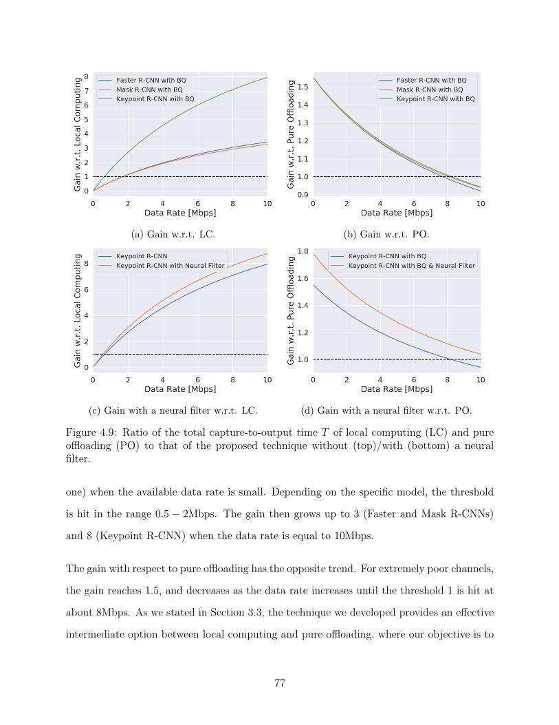
(a) Gain w.r.t. LC. (b) Gain w.r.t. PO.

(c) Gain with a neural filter w.r.t. LC. (d) Gain with a neural filter w.r.t. PO.

Figure 4.9: Ratio of the total capture-to-output time T of local computing (LC) and pureoffloading (PO) to that of the proposed technique without (top)/with (bottom) a neuralfilter.

one) when the available data rate is small. Depending on the specific model, the threshold

is hit in the range 0.5 − 2Mbps. The gain then grows up to 3 (Faster and Mask R-CNNs)

and 8 (Keypoint R-CNN) when the data rate is equal to 10Mbps.

The gain with respect to pure offloading has the opposite trend. For extremely poor channels,

the gain reaches 1.5, and decreases as the data rate increases until the threshold 1 is hit at

about 8Mbps. As we stated in Section 3.3, the technique we developed provides an effective

intermediate option between local computing and pure offloading, where our objective is to

77

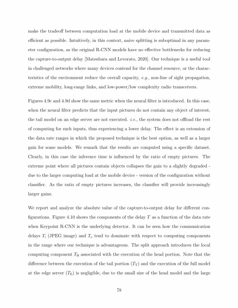
make the tradeoff between computation load at the mobile device and transmitted data as

efficient as possible. Intuitively, in this context, naive splitting is suboptimal in any param-

eter configuration, as the original R-CNN models have no effective bottlenecks for reducing

the capture-to-output delay [Matsubara and Levorato, 2020]. Our technique is a useful tool

in challenged networks where many devices contend for the channel resource, or the charac-

teristics of the environment reduce the overall capacity, e.g., non-line of sight propagation,

extreme mobility, long-range links, and low-power/low complexity radio transceivers.

Figures 4.9c and 4.9d show the same metric when the neural filter is introduced. In this case,

when the neural filter predicts that the input pictures do not contain any object of interest,

the tail model on an edge server are not executed. i.e., the system does not offload the rest

of computing for such inputs, thus experiencing a lower delay. The effect is an extension of

the data rate ranges in which the proposed technique is the best option, as well as a larger

gain for some models. We remark that the results are computed using a specific dataset.

Clearly, in this case the inference time is influenced by the ratio of empty pictures. The

extreme point where all pictures contain objects collapses the gain to a slightly degraded -

due to the larger computing load at the mobile device - version of the configuration without

classifier. As the ratio of empty pictures increases, the classifier will provide increasingly

larger gains.

We report and analyze the absolute value of the capture-to-output delay for different con-

figurations. Figure 4.10 shows the components of the delay T as a function of the data rate

when Keypoint R-CNN is the underlying detector. It can be seen how the communication

delays Ti (JPEG image) and To tend to dominate with respect to computing components

in the range where our technique is advantageous. The split approach introduces the local

computing component TH associated with the execution of the head portion. Note that the

difference between the execution of the tail portion (TT) and the execution of the full model

at the edge server (TE) is negligible, due to the small size of the head model and the large

78

Figure 4.10: Component-wise delays of original and our Keypoint R-CNNs in different datarates. LC: Local Computing, PO: Pure Offloading, SC: Split Computing, SCNF: SplitComputing with Neural Filter

computing capacity of the edge server. The figure also shows, while the reduction in the

total capture-to-output delay is perceivable, the extra classifier imposes a small additional

computing load compared to the head model with bottleneck.

4.6 Conclusions

This chapter discusses the challenges in deploying complex object detection models and

presents a technique to efficiently split deep neural networks for object detection. The core

idea is to achieve in-network compression introducing a bottleneck layer in the early stages

of the backbone network. The output of the bottleneck is quantized and then sent to the

edge server, which executes some layers to reconstruct the original output of head model

and the tail portion. Additionally, we embed in the head model a low-complexity classifier

which acts as a filter to eliminate pictures that do not contain objects of interest, further

improving efficiency. We demonstrate that our generalized head network distillation can

79

lead to models achieving state-of-the-art performance while reducing total inference time in

parameter regions where local and edge computing provide unsatisfactory performance.

80

Chapter 5

Supervised Compression for Split

Computing

5.1 Introduction

With the abundance of smartphones, autonomous drones, and other intelligent devices, ad-

vanced computing systems for machine learning applications have become evermore impor-

tant [Shi et al., 2016, Chen and Ran, 2019]. Machine learning models are frequently deployed

on low-powered devices for reasons of computational efficiency or data privacy [Sandler et al.,

2018, Howard et al., 2019]. However, deploying conventional computer vision or NLP models

on such hardware raises a computational challenge, as powerful deep neural networks are

often too energy-consuming to be deployed on such weak mobile devices [Eshratifar et al.,

2019a].

An alternative to carrying out the deep learning model’s operation on the low-powered

device is to send compressed data to an edge server that takes care of the heavy com-

putation instead. However, recent neural or classical compression algorithms are either

81

Input Compressor DecompressorReconstructed

InputCompressed

Input

Full Inference Model

“Zebra”

Prediction

Input Encoder DecoderDecoded FeatureCompressed

Feature

Pruned Inference Model

“Zebra”

Prediction

(a) Input Compression for Full Offloading

(b) Supervised Compression for Split Computing

Mobile Device Cloud/Edge ServerCommunication

Figure 5.1: Image classification with input compression (top) vs. our proposed supervisedcompression for split computing (bottom). While the former approach fully reconstructsthe image, our approach learns an intermediate compressible representation suitable for thesupervised task.

resource-intensive [Singh et al., 2020, Dubois et al., 2021] and/or optimized for perceptual

quality [Balle et al., 2017, Minnen et al., 2018], and therefore much of the information trans-

mitted is redundant for the machine learning task [Choi and Han, 2020] (see Fig. 5.1). A

better solution is to therefore split the neural network [Kang et al., 2017] into the two se-

quences so that some elementary feature transformations are applied by the first sequence of

the model on the weak mobile (local) device. Then, intermediate, informative features are

transmitted through a wireless communication channel to the edge server that processes the

bulk part of the computation (the second sequence of the model) [Eshratifar et al., 2019b,

Matsubara et al., 2019].

Traditional split computing approaches transmit intermediate features by either reducing

channels in convolution layers [Kang et al., 2017] or truncating them to a lower arithmetic

precision [Matsubara et al., 2020, Shao and Zhang, 2020, Matsubara and Levorato, 2021].

Since the models were not “informed” about such truncation steps during training oftentimes

82

leads to substantial performance degradation. This raises the question of whether learnable

end-to-end data compression pipelines can be designed to both truncate and entropy-code

the involved early-stage features.

In this work, we propose such a neural feature compression approach by drawing on varia-

tional inference-based data compression [Balle et al., 2018, Singh et al., 2020]. Our architec-

ture resembles the variational information bottleneck objective [Alemi et al., 2017] and relies

on an encoder, a “prior” on the bottleneck state, and a decoder that leads to a supervised

loss (see Fig. 5.1). At inference time, we discretize the encoder’s output and use our learned

prior as a model for entropy coding intermediate features. The decoder reconstructs the

feature vector losslessly from the binary bitstring and carries out the subsequent supervised

machine learning task. Crucially, we combine this feature compression approach with knowl-

edge distillation, where a teacher model provides the training data as well as parts of the

trained architecture.1

In more detail, our main contributions are as follows:

• We propose a new training objective for feature compression in split computing that

allows us to use a learned entropy model for bottleneck quantization in conjunction

with knowledge distillation.

• Our approach significantly outperforms seven strong baselines from the split computing

and (neural) image compression literature in terms of rate-distortion performance (with

distortion measuring a supervised error) and in terms of end-to-end latency.

• Moreover, we show that a single encoder network can serve multiple supervised tasks,

including classification, object detection, and semantic segmentation.

1Code and models are available at https://github.com/yoshitomo-matsubara/sc2-benchmark

83

5.2 Method

After providing an overview of the setup (Section 5.2.1) we describe our distillation and

feature compression approach (Section 5.2.2) and our procedure to fine-tune the model to

other supervised downstream tasks (Section 5.2.3).

5.2.1 Overview

Our goal is to learn a lightweight, communication-efficient feature extractor for supervised

downstream applications. We thereby transmit intermediate feature activations between

two distinct portions of a neural network. The first part is deployed on a low-power mobile

device, and the second part on a compute-capable edge server. Intermediate feature repre-

sentations are compressed and transmitted between the mobile device and the edge server

using discretization and subsequent lossless entropy coding.

In order to learn good compressible feature representations, we combine two ideas: knowledge

distillation and neural data compression via learned entropy coding. First, we train a large

teacher network on a data set of interest to teach a smaller student model. We assume that

the features that the teacher model learns are helpful for other downstream tasks. Then,

we train a lightweight student model to match the teacher model’s intermediate features

(Section 5.2.2) with minimal performance loss. Finally, we fine-tune the student model to

different downstream tasks (Section 5.2.3). Note that the training process is done offline.

The teacher network realizes a deterministic mapping x 7→ h 7→ y, where x are the input

data, y are the targets, and h are some intermediate feature representations of the teacher

network. We assume that the teacher model is too large to be executed on the mobile device.

The main idea is to replace the teacher model’s mapping x 7→ h with a student model (i.e.,

the new targets become the teacher model’s intermediate feature activations). To facilitate

84

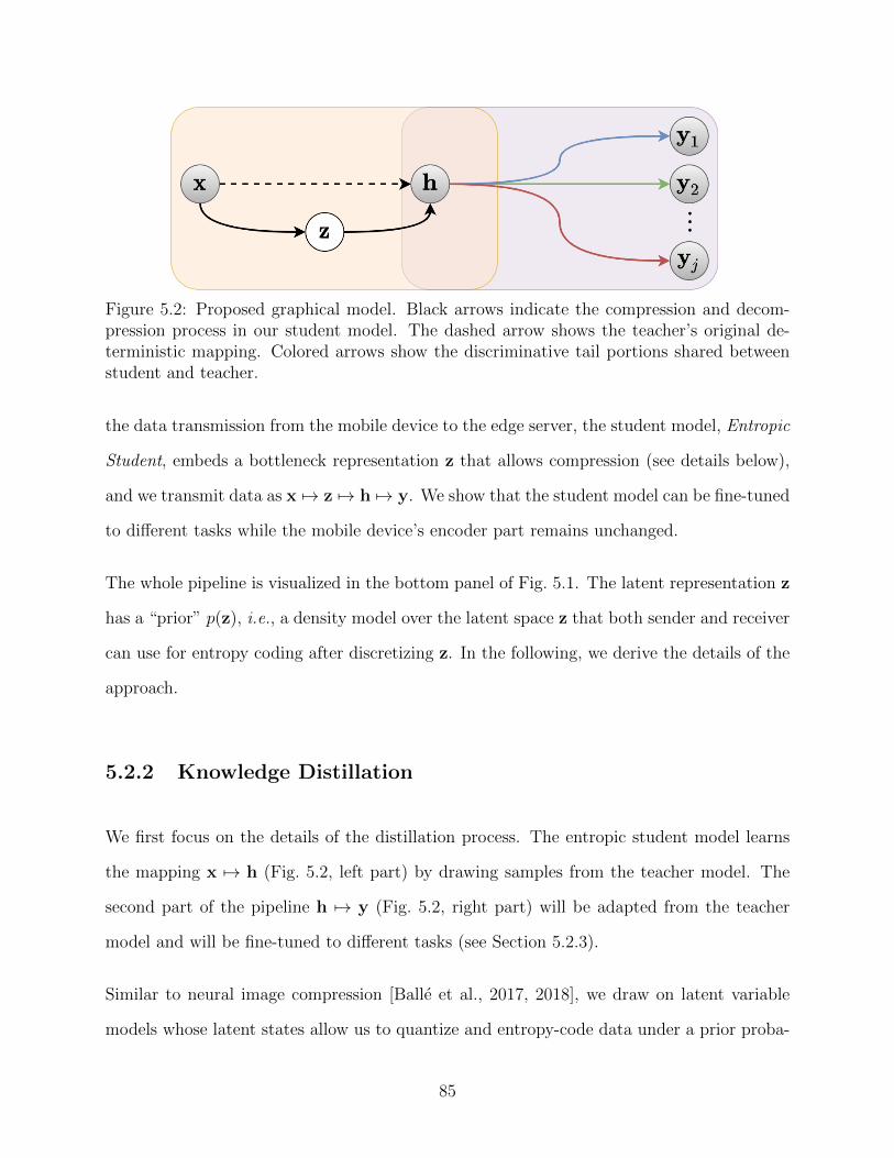
Figure 5.2: Proposed graphical model. Black arrows indicate the compression and decom-pression process in our student model. The dashed arrow shows the teacher’s original de-terministic mapping. Colored arrows show the discriminative tail portions shared betweenstudent and teacher.

the data transmission from the mobile device to the edge server, the student model, Entropic

Student, embeds a bottleneck representation z that allows compression (see details below),

and we transmit data as x 7→ z 7→ h 7→ y. We show that the student model can be fine-tuned

to different tasks while the mobile device’s encoder part remains unchanged.

The whole pipeline is visualized in the bottom panel of Fig. 5.1. The latent representation z

has a “prior” p(z), i.e., a density model over the latent space z that both sender and receiver

can use for entropy coding after discretizing z. In the following, we derive the details of the

approach.

5.2.2 Knowledge Distillation

We first focus on the details of the distillation process. The entropic student model learns

the mapping x 7→ h (Fig. 5.2, left part) by drawing samples from the teacher model. The

second part of the pipeline h 7→ y (Fig. 5.2, right part) will be adapted from the teacher

model and will be fine-tuned to different tasks (see Section 5.2.3).

Similar to neural image compression [Balle et al., 2017, 2018], we draw on latent variable

models whose latent states allow us to quantize and entropy-code data under a prior proba-

85

Input Teacher (Pretrained)

1st stage: Student w/ Bottleneck

Input Teacher (Pretrained)

2nd stage: Student w/ Bottleneck

Frozen Frozen

FrozenFrozen

Hard-target:“Zebra”

Soft-target:

Figure 5.3: Our two-stage training approach. Left: training the student model (bottom)with targets h and tail architecture obtained from teacher (top) (Section 5.2.2). Right:fine-tuning the decoder and tail portion with fixed encoder (Section 5.2.3).

bility model. In contrast to neural image compression, our approach is supervised. As such,

it mathematically resembles the deep Variational Information Bottleneck [Alemi et al., 2017]

(which was designed for adversarial robustness rather than compression).

Distillation Objective. We assume a stochastic encoder q(z|x), a decoder p(h|z), and

a density model (“prior”) p(z) in the latent space. Specific choices are detailed below.

Similar to [Alemi et al., 2017], we maximize mutual information between z and h (making

the compressed bottleneck state z as informative as possible about the supervised target h)

while minimizing the mutual information between the input x and z (thus “compressing

away” all the irrelevant information that does not immediately serve the supervised goal).

The objective for a given training pair (x,h) provided by the teacher model is

L(x,h) = −Eqθ(z|x)[log pϕ(h|z)︸ ︷︷ ︸distortion

+β log pϕ(z)︸ ︷︷ ︸rate

]. (5.1)

Before discussing the rate and distortion terms, we specify and simplify this loss function

further. Above, the decoder p(h|z) = N (h; gϕ(z), I) is chosen as a conditional Gaussian

centered around a deterministic prediction gϕ(z). Following the neural image compression

literature [Balle et al., 2017, 2018], the encoder is chosen to be a unit-width box function

86

qθ(z|x) = U(fθ(x)−12, fθ(x)+

12) centered around a neural network prediction fθ(x). Using the

reparameterization trick [Kingma and Welling, 2014], Eq. 5.1 can be optimized via stochastic

gradient descent 2

L(x,h) = 12||h− gϕ (fθ (x) + ϵ) ||22︸ ︷︷ ︸

distortion

−β log pϕ(fθ(x) + ϵ)︸ ︷︷ ︸rate

, ϵ ∼ Unif(−12, 12). (5.2)

Once the model is trained, we discretize the latent state z = ⌊fθ(x)⌉ (where ⌊·⌉ denotes the

rounding operation) to allow for entropy coding under pϕ(z). By injecting noise from a box-

shaped distribution of width one, we simulate the rounding operation during training. The

entropy model or prior pϕ(z) is adopted from the neural image compression literature [Balle

et al., 2018]; it is a learnable prior with tuning parameters ϕ. The prior factorizes over all

dimensions of z, allowing for efficient and parallel entropy coding.

Supervised Rate-Distortion Tradeoff. Similar to unsupervised data compression, our

approach results in a rate-distortion tradeoff: the more aggressively we compress the latent

representation z, the more the predictive performance will deteriorate. In contrast, the more

bits we are willing to invest for compressing z, the more predictive strength our model will

maintain. The goal will be to perform well on the unavailable tradeoff between rate and

distortion.

The first term in Eq. 5.1 measures the supervised distortion, as it expresses the average

prediction error under the coding procedure of first mapping x to z and then z to h. In con-

trast, the second term measures the coding costs as the cross-entropy between the empirical

distribution of zi and the prior distribution pϕ(z) according to information theory [Cover,

1999]. The tradeoff is determined by the Lagrange multiplier β.

As a particular instantiation of an information bottleneck framework [Alemi et al., 2017], Singh

2For better convergence, we follow [Matsubara and Levorato, 2021] and leverage intermediate represen-tations from frozen layers besides h as illustrated in Fig. 5.3 (left).

87

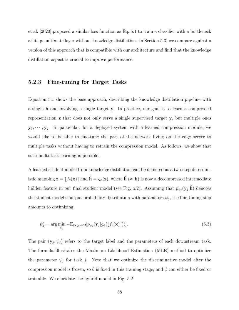
et al. [2020] proposed a similar loss function as Eq. 5.1 to train a classifier with a bottleneck

at its penultimate layer without knowledge distillation. In Section 5.3, we compare against a

version of this approach that is compatible with our architecture and find that the knowledge

distillation aspect is crucial to improve performance.

5.2.3 Fine-tuning for Target Tasks

Equation 5.1 shows the base approach, describing the knowledge distillation pipeline with

a single h and involving a single target y. In practice, our goal is to learn a compressed

representation z that does not only serve a single supervised target y, but multiple ones

y1, · · · ,yj. In particular, for a deployed system with a learned compression module, we

would like to be able to fine-tune the part of the network living on the edge server to

multiple tasks without having to retrain the compression model. As follows, we show that

such multi-task learning is possible.

A learned student model from knowledge distillation can be depicted as a two-step determin-

istic mapping z = ⌊fθ(x)⌉ and h = gϕ(z), where h (≈ h) is now a decompressed intermediate

hidden feature in our final student model (see Fig. 5.2). Assuming that pψj(yj|h) denotes

the student model’s output probability distribution with parameters ψj, the fine-tuning step

amounts to optimizing

ψ∗j = argmin

ψj

−E(x,y)∼D[pψj(yj|gϕ(⌊fθ(x)⌉))]. (5.3)

The pair (yj, ψj) refers to the target label and the parameters of each downstream task.

The formula illustrates the Maximum Likelihood Estimation (MLE) method to optimize

the parameter ψj for task j. Note that we optimize the discriminative model after the

compression model is frozen, so θ is fixed in this training stage, and ϕ can either be fixed or

trainable. We elucidate the hybrid model in Fig. 5.2.

88

For fine-tuning the student model with the frozen encoder, we leverage a teacher model

again. For image classification, we apply a standard knowledge distillation technique [Hin-

ton et al., 2014] to achieve better model accuracy by distilling the knowledge in the teacher

model into our student model. Specifically, we fine-tune the student model by minimizing

a weighted sum of two losses: 1) cross-entropy loss between the student model’s class prob-

ability distribution and one-hot vector (hard -target), and 2) Kullback-Leibler divergence

between softened class probability distributions from both the student and teacher models.

Similarly, having frozen the encoder, we can fine-tune different models for different down-

stream tasks reusing the trained entropic student model (classifier) as their backbone, which

will be demonstrated in Section 5.3.4.

5.3 Experiments

Using torchdistill [Matsubara, 2021], we designed different experiments and studied various

models based on both principles of split-computing (partial offloading) and edge computing

(full offloading). We used ResNet-50 [He et al., 2016] as a base model, which, besides image

classification, is also widely used as a backbone for different vision tasks such as object

detection [He et al., 2017a, Lin et al., 2017b] and semantic segmentation [Chen et al., 2017c].

In all experiments, we empirically show that our approach leads to better supervised rate-

distortion performance.

5.3.1 Baselines

In this study, we use seven baseline methods categorized into either input compression or

feature compression.

89

Input compression (IC). A conventional implementation of the edge computing paradigm

is to transmit the compressed image directly to the edge server, where all the tasks are then

executed. We consider five baselines referring to this “input compression” scenario: JPEG,

WebP [Google], BPG [Bellard], and two neural image compression methods (factorized prior

and mean-scale hyperprior) [Balle et al., 2018, Minnen et al., 2018] based on Compres-

sAI [Begaint et al., 2020]. The latter approach is currently considered state of the art in

image compression models (without autoregressive structure) [Minnen et al., 2018, Minnen

and Singh, 2020, Yang et al., 2020c]. We evaluate each model’s performance in terms of

the rate-distortion curve by setting different quality values for JPEG, WebP, and BPG and

Lagrange multiplier β for neural image compression.

Feature compression (FC). Split computing baselines [Matsubara et al., 2020, Shao

and Zhang, 2020] correspond to reducing the bottleneck data size with channel reduction

and bottleneck quantization referred to as CR+BQ (quantizes 32-bit floating-point to 8-bit

integer) [Jacob et al., 2018]. Matsubara and Levorato [2021], Matsubara et al. [2020] report

that bottleneck quantization did not lead to significant accuracy loss. To control the rate-

distortion tradeoff, we design bottlenecks with a different number of output channels in a

convolution layer to control the bottleneck data size, train the bottleneck-injected models

and quantize the bottleneck after the training session.

Our final baseline in this work is an end-to-end approach towards learning compressible fea-

tures for a single task similar to Singh et al. [2020] (for brevity, we will cite their reference).

Their originally proposed approach focuses only on classification and introduces the com-

pressible bottleneck to the penultimate layer. In the considered setting, such design leads

to an overwhelming workload for the mobile/local device: for example, in terms of model

parameters, about 92% of the ResNet-50 [He et al., 2016] parameters would be deployed on

the weaker, mobile device. To make this approach compatible with our setting, we apply

their approach to our architecture; that is, we directly train our entropic student model

90

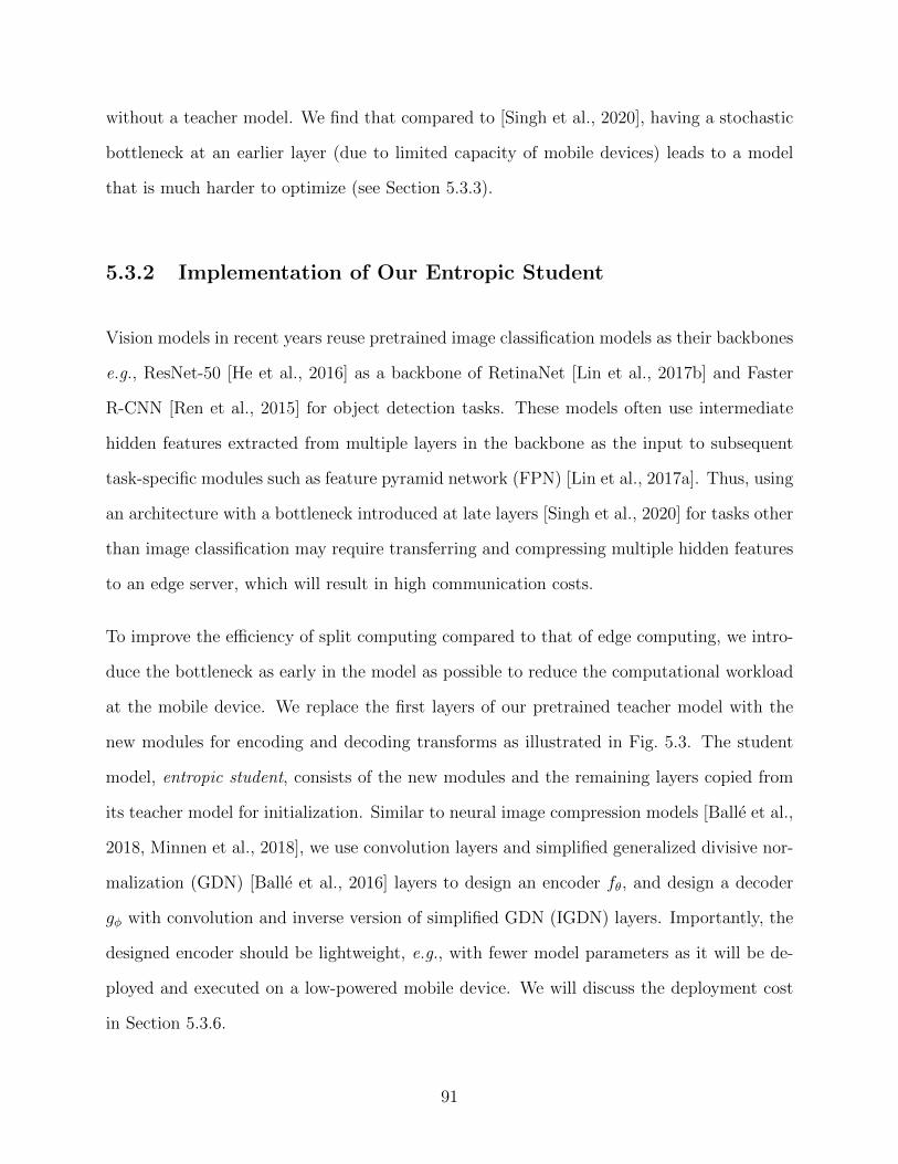
without a teacher model. We find that compared to [Singh et al., 2020], having a stochastic

bottleneck at an earlier layer (due to limited capacity of mobile devices) leads to a model

that is much harder to optimize (see Section 5.3.3).

5.3.2 Implementation of Our Entropic Student

Vision models in recent years reuse pretrained image classification models as their backbones

e.g., ResNet-50 [He et al., 2016] as a backbone of RetinaNet [Lin et al., 2017b] and Faster

R-CNN [Ren et al., 2015] for object detection tasks. These models often use intermediate

hidden features extracted from multiple layers in the backbone as the input to subsequent

task-specific modules such as feature pyramid network (FPN) [Lin et al., 2017a]. Thus, using

an architecture with a bottleneck introduced at late layers [Singh et al., 2020] for tasks other

than image classification may require transferring and compressing multiple hidden features

to an edge server, which will result in high communication costs.

To improve the efficiency of split computing compared to that of edge computing, we intro-

duce the bottleneck as early in the model as possible to reduce the computational workload

at the mobile device. We replace the first layers of our pretrained teacher model with the

new modules for encoding and decoding transforms as illustrated in Fig. 5.3. The student

model, entropic student, consists of the new modules and the remaining layers copied from

its teacher model for initialization. Similar to neural image compression models [Balle et al.,

2018, Minnen et al., 2018], we use convolution layers and simplified generalized divisive nor-

malization (GDN) [Balle et al., 2016] layers to design an encoder fθ, and design a decoder

gϕ with convolution and inverse version of simplified GDN (IGDN) layers. Importantly, the

designed encoder should be lightweight, e.g., with fewer model parameters as it will be de-

ployed and executed on a low-powered mobile device. We will discuss the deployment cost

in Section 5.3.6.

91

Different from bottleneck designs in the prior studies on split computing [Matsubara and

Levorato, 2021, Matsubara et al., 2020], we control the trade-off between bottleneck data

size and model accuracy with the β value in the rate-distortion loss function (See Eq. 5.2).

5.3.3 Image Classification

We first discuss the rate-distortion performance of our and baseline models using a large-scale

image classification dataset. Specifically, we use ImageNet (ILSVRC 2012) [Russakovsky

et al., 2015], that consists of 1.28 million training and 50,000 validation samples. As is

standard, we train the models on the training split and report the top-1 accuracy on the

validation split. Using ResNet-50 [He et al., 2016] pre-trained on ImageNet as a teacher

model, we replace all the layers before its second residual block with our encoder and decoder

to compose our entropic student model. The introduced encoder-decoder modules are trained

to approximate h in Eq. 5.2, which is the output of the corresponding residual block in the

teacher model (original ResNet-50) in the first stage, and then we fine-tune the student

model as described in Section 5.2. We provide more details of training configurations (e.g.,

hyperparameters) in the supplementary material.

Figure 5.4 presents supervised rate-distortion curves of ResNet-50 with various compression

approaches, where the x-axis shows the average data size, and the y-axis the supervised

performance. We note that the input tensor shape for ResNet-50 as an image classifier is

3 × 224 × 224. For image compression, the result shows the considered neural compression

models, factorized prior [Balle et al., 2018] and mean-scale hyperprior [Minnen et al., 2018],

consistently outperform JPEG and WebP compression in terms of rate-distortion curves

in the image classification task. A popular approach used in split computing studies, the

combination of channel reduction and bottleneck quantization (CR+BQ) [Matsubara and

Levorato, 2021], seems slightly better than JPEG compression but not as accurate as those

92

100 101

Compressed Data Size [KByte]

50

55

60

65

70

75

80

Accuracy

[%]

IC: JPEG

IC: WebP [Google]

IC: BPG [Bellard]

IC: Factorized Prior [Balle et al. 2018]

IC: Mean-scale Hyperprior [Minnen et al. 2018]

FC: CR + BQ [Matsubara & Levorato 2020]

FC: Compressive Feature [Singh et al. 2020]

FC: Our Supervised Compression

Figure 5.4: Rate-distortion (accuracy) curves of ResNet-50 as base model for ImageNet(ILSVRC 2012).

with the neural image compression models.

Among all the configurations in the figure, our model trained by the two-stage method

performs the best. We also trained our model without teacher model, which in essence

corresponds to [Singh et al., 2020]. The resulting RD curve is significantly worse, which we

attribute to two possible effects: first, it is widely acknowledged that knowledge distillation

generally finds solutions that generalize better. Second, having a stochastic bottleneck at an

earlier layer may make it difficult for the end-to-end training approach to optimize.

5.3.4 Object Detection and Semantic Segmentation

As suggested by He et al. [2019], image classifiers pre-trained on the ImageNet dataset [Rus-

sakovsky et al., 2015] speed up the convergence of training on downstream tasks. Reusing the

proposed model pre-trained on the ImageNet dataset, we further discuss the rate-distortion

performance on two downstream tasks: object detection and semantic segmentation. Specif-

ically, we train RetinaNet [Lin et al., 2017b] and DeepLabv3 [Chen et al., 2017c], using

93

101 102

Compressed Data Size [KByte]

20

22

24

26

28

30

32

34

36

38

mAP[%

]

IC: JPEG

IC: WebP [Google]

IC: BPG [Bellard]

IC: Factorized Prior [Balle et al. 2018]

IC: Mean-scale Hyperprior [Minnen et al. 2018]

FC: CR + BQ [Matsubara & Levorato 2020]

FC: Compressive Feature [Singh et al. 2020]

FC: Our Supervised Compression

Figure 5.5: Rate-distortion (BBox mAP) curves of RetinaNet with ResNet-50 and FPN asbase backbone for COCO 2017.

101 102

Compressed Data Size [KByte]

50

52

54

56

58

60

62

64

66

68

mIoU

IC: JPEG

IC: WebP [Google]

IC: BPG [Bellard]

IC: Factorized Prior [Balle et al. 2018]

IC: Mean-scale Hyperprior [Minnen et al. 2018]

FC: CR + BQ [Matsubara & Levorato 2020]

FC: Compressive Feature [Singh et al. 2020]

FC: Our Supervised Compression

Figure 5.6: Rate-distortion (Seg mIoU) curves of DeepLabv3 with ResNet-50 as base back-bone for COCO 2017.

94

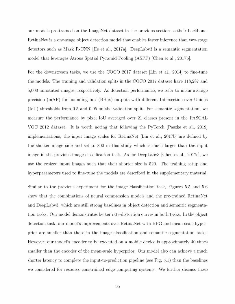
our models pre-trained on the ImageNet dataset in the previous section as their backbone.

RetinaNet is a one-stage object detection model that enables faster inference than two-stage

detectors such as Mask R-CNN [He et al., 2017a]. DeepLabv3 is a semantic segmentation

model that leverages Atrous Spatial Pyramid Pooling (ASPP) [Chen et al., 2017b].

For the downstream tasks, we use the COCO 2017 dataset [Lin et al., 2014] to fine-tune

the models. The training and validation splits in the COCO 2017 dataset have 118,287 and

5,000 annotated images, respectively. As detection performance, we refer to mean average

precision (mAP) for bounding box (BBox) outputs with different Intersection-over-Unions

(IoU) thresholds from 0.5 and 0.95 on the validation split. For semantic segmentation, we

measure the performance by pixel IoU averaged over 21 classes present in the PASCAL

VOC 2012 dataset. It is worth noting that following the PyTorch [Paszke et al., 2019]

implementations, the input image scales for RetinaNet [Lin et al., 2017b] are defined by

the shorter image side and set to 800 in this study which is much larger than the input

image in the previous image classification task. As for DeepLabv3 [Chen et al., 2017c], we

use the resized input images such that their shorter size is 520. The training setup and

hyperparameters used to fine-tune the models are described in the supplementary material.

Similar to the previous experiment for the image classification task, Figures 5.5 and 5.6

show that the combinations of neural compression models and the pre-trained RetinaNet

and DeepLabv3, which are still strong baselines in object detection and semantic segmenta-

tion tasks. Our model demonstrates better rate-distortion curves in both tasks. In the object

detection task, our model’s improvements over RetinaNet with BPG and mean-scale hyper-

prior are smaller than those in the image classification and semantic segmentation tasks.

However, our model’s encoder to be executed on a mobile device is approximately 40 times

smaller than the encoder of the mean-scale hyperprior. Our model also can achieve a much

shorter latency to complete the input-to-prediction pipeline (see Fig. 5.1) than the baselines

we considered for resource-constrained edge computing systems. We further discuss these

95

aspects in Sections 5.3.6 and 5.3.7.

5.3.5 Bitrate Allocation of Latent Representations

This section discusses the difference between the representations of bottlenecks in neural

image compression and our models. We are interested in which element of the bottlenecks

allocates more bits in the latent representation z. Bottlenecks in neural image compression

models will allocate many bits to some unique area in an image to preserve all its charac-

teristics in the reconstructed image. On the other hand, those in our models are trained to

mimic the feature representations in their teacher model, thus expected to allocate more bits

to areas useful for the target task.

Figure 5.7 shows visualizations of the normalized bitrate allocations for a few sample images.

The 2nd column of the figure corresponds to the bottleneck in a neural image compression

model prioritizing the images’ backgrounds such as catcher’s zone and glasses. Interestingly,

our bottleneck representation (the 3rd column) seems to eliminate the difference between

the two backgrounds and focuses on objects in the images such as persons and soccer ball.

Moreover, the bottleneck eliminates a digital watermark at the top left in the first image,

which is most likely not critical for the target task, while the one in the neural compression

model noticeably distinguishes the logo from the background.

5.3.6 Deployment Cost on Mobile Devices

In Sections 5.3.3 and 5.3.4, we discussed the trade-off between transferred data size and model

accuracy with the visualization of rate-distortion curves. While improving the rate-distortion

curves is essential for resource-constrained edge computing systems, it is also important to

reduce the computational burden allocated to the mobile device that often have more severe

96

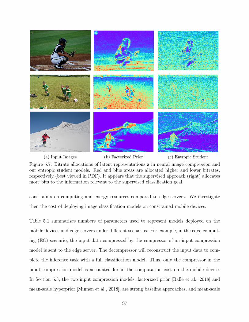
(a) Input Images (b) Factorized Prior (c) Entropic Student

Figure 5.7: Bitrate allocations of latent representations z in neural image compression andour entropic student models. Red and blue areas are allocated higher and lower bitrates,respectively (best viewed in PDF). It appears that the supervised approach (right) allocatesmore bits to the information relevant to the supervised classification goal.

constraints on computing and energy resources compared to edge servers. We investigate

then the cost of deploying image classification models on constrained mobile devices.

Table 5.1 summarizes numbers of parameters used to represent models deployed on the

mobile devices and edge servers under different scenarios. For example, in the edge comput-

ing (EC) scenario, the input data compressed by the compressor of an input compression

model is sent to the edge server. The decompressor will reconstruct the input data to com-

plete the inference task with a full classification model. Thus, only the compressor in the

input compression model is accounted for in the computation cost on the mobile device.

In Section 5.3, the two input compression models, factorized prior [Balle et al., 2018] and

mean-scale hyperprior [Minnen et al., 2018], are strong baseline approaches, and mean-scale

97

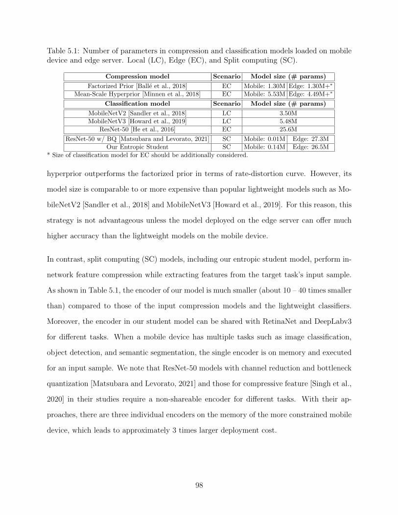
Table 5.1: Number of parameters in compression and classification models loaded on mobiledevice and edge server. Local (LC), Edge (EC), and Split computing (SC).

Compression model Scenario Model size (# params)

Factorized Prior [Balle et al., 2018] EC Mobile: 1.30M Edge: 1.30M+∗

Mean-Scale Hyperprior [Minnen et al., 2018] EC Mobile: 5.53M Edge: 4.49M+∗

Classification model Scenario Model size (# params)

MobileNetV2 [Sandler et al., 2018] LC 3.50MMobileNetV3 [Howard et al., 2019] LC 5.48M

ResNet-50 [He et al., 2016] EC 25.6M

ResNet-50 w/ BQ [Matsubara and Levorato, 2021] SC Mobile: 0.01M Edge: 27.3MOur Entropic Student SC Mobile: 0.14M Edge: 26.5M

* Size of classification model for EC should be additionally considered.

hyperprior outperforms the factorized prior in terms of rate-distortion curve. However, its

model size is comparable to or more expensive than popular lightweight models such as Mo-

bileNetV2 [Sandler et al., 2018] and MobileNetV3 [Howard et al., 2019]. For this reason, this

strategy is not advantageous unless the model deployed on the edge server can offer much

higher accuracy than the lightweight models on the mobile device.

In contrast, split computing (SC) models, including our entropic student model, perform in-

network feature compression while extracting features from the target task’s input sample.

As shown in Table 5.1, the encoder of our model is much smaller (about 10 – 40 times smaller

than) compared to those of the input compression models and the lightweight classifiers.

Moreover, the encoder in our student model can be shared with RetinaNet and DeepLabv3

for different tasks. When a mobile device has multiple tasks such as image classification,

object detection, and semantic segmentation, the single encoder is on memory and executed

for an input sample. We note that ResNet-50 models with channel reduction and bottleneck

quantization [Matsubara and Levorato, 2021] and those for compressive feature [Singh et al.,

2020] in their studies require a non-shareable encoder for different tasks. With their ap-

proaches, there are three individual encoders on the memory of the more constrained mobile

device, which leads to approximately 3 times larger deployment cost.

98

Table 5.2: End-to-end latency to complete input-to-prediction pipeline for resource-constrained edge computing systems illustrated in Fig. 5.1, using RPI4/JTX2, LoRa andES. The breakdowns are available in the supplementary material.

Approach RPI4 −→ ES JTX2 −→ ES

JPEG + ResNet-50 2.35 sec 2.34 secWebP + ResNet-50 1.83 sec 1.84 secBPG + ResNet-50 2.46 sec 2.41 sec

Factorized Prior + ResNet-50 2.43 sec 2.22 secMean-Scale Hyperprior + ResNet-50 2.24 sec 1.92 sec

ResNet-50 w/ BQ 2.27 sec 2.25 sec

Our Entropic Student 0.972 sec 0.904 sec

5.3.7 End-to-End Prediction Latency Evaluation

To compare the prediction latency with the different approaches, we deploy the encoders on

two different mobile devices: Raspberry Pi 4 (RPI4) and NVIDIA Jetson TX2 (JTX2). As

an edge server (ES), we use a desktop computer with an NVIDIA GeForce RTX 2080 Ti,

assuming the use of LoRa [Samie et al., 2016] for low-power communications (maximum data

rate is 37.5 Kbps). For all the considered approaches, we use the data points with about 74%

accuracy in Fig. 5.4, and the end-to-end latency is the sum of 1) execution time to encode

an input image on RPI4/JTX2, 2) delay to transfer the encoded data from RPI4/JTX2 to

ES, and 3) execution time to decode the compressed data and complete inference on ES.

Table 5.2 shows that our approach reduces the end-to-end prediction latency by 47 – 62%

compared to the baselines. The encoding time and communication delay are dominant in the

end-to-end latency while the execution time on ES is negligible. For both the experimental

configurations (RPI4 −→ ES and JTX2 −→ ES), the breakdowns of the end-to-end latency

are illustrated in the supplementary material.

99

5.4 Conclusions

This work adopts ideas from knowledge distillation and neural image compression to achieve

feature compression for supervised tasks. Our approach leverages a teacher model to intro-

duce a stochastic bottleneck and a learnable prior for entropy coding at its early stage of a

student model (namely, Entropic Student). The framework reduces the computational bur-

den on the weak mobile device by offloading most of the computation to a computationally

powerful cloud/edge server, and the single encoder in our entropic student can serve multiple

downstream tasks. The experimental results show the improved supervised rate-distortion

performance for three different vision tasks and the shortened end-to-end prediction latency,

compared to various (neural) image compression and feature compression baselines.

100

Chapter 6

Conclusion

6.1 Summary

In this dissertation, we are focused on split computing for resource-constrained edge com-

puting systems and proposed various methods to make split computing a reasonable inter-

mediate option between local and edge computing, empirically showing effectiveness of the

approaches through extensive amount of large-scale experiments.

In Chapter 2, we presented overview of local, edge, and split computing and background of

deep learning for mobile application. We then put our focus on split computing and shared a

survey of related studies, highlighting the need for bottlenecks introduced to DNN models in

order to achieve efficient split computing for resource-constrained edge computing systems.

In Chapter 3, we discussed in detail the structure of our designed student models and head

network distillation (HND) to achieve in-network compression while placing limited amount

of computing load to mobile devices and preserve accuracy. Using the ImageNet dataset,

we discuss the effectiveness of the proposed HND in terms of model accuracy and training

101

cost compared to other end-to-end training methods. We also show how bottlenecks with a

quantization technique can aggressively reduce data size without significant accuracy loss.

With the quantized bottlenecks, our experimental results for simulated and real platforms

show that the proposed framework of split DNN with introduce bottlenecks can achieve

shorter end-to-end prediction latency for resource-constrained edge computing systems.

In Chapter 4, we put our focus on object detection tasks. Analyzing complex object detec-

tion models in terms of layer-wise output data size and model complexity, we found that no

effective splitting point exists in such models. Also, such modern object detection models has

a unique property, that is leveraging outputs of multiple intermediate layers to achieve multi-

scale object detection, which makes split computing more challenging for object detection

tasks. To address the problems, we proposed generalized HND (GHND), that leverages mul-

tiple intermediate feature representations from both teacher and student models to minimize

model accuracy loss with respect to the teacher model. Besides the bottlenecks introduced

to the student model, we introduced a lightweight neural filter to its head model for filtering

out images containing no objects of interest before offloading so that the model can terminate

the inference for such images at mobile device side.

In Chapter 5, we introduced a concept of supervised compression and proposed a new tradeoff

metric for split computing to consider not only data size and model accuracy (rate-distortion

tradeoff) but also encoder size as we should minimize encoder size for weak local devices

while improving rate-distortion tradeoff. Based on the concept and the new tradeoff, we

leveraged the ideas from neural image compression and knowledge distillation and proposed

Entropic Student, a new supervised compression approach for split computing. Through

large-scale experiments for image classification, object detection, and semantic segmentation,

we empirically showed that our proposed approach significantly outperforms all the strong

baseline methods in terms of R-D tradeoff while our single lightweight encoder serves multiple

downstream tasks without being fine-tuned to each of the tasks.

102

6.2 Further Research Challenges

For future work, we open up some of the further research challenges in split computing.

Optimization of Bottleneck Design and Placement

The study of the architecture and placement of the bottleneck in a DNN model is also of

considerable importance. Important metrics include: (i) bottleneck data size (or compres-

sion rate), (ii) complexity of head model executed on mobile device, and (iii) resulting model

accuracy. As a principle, the smaller the bottleneck representation is, the lower the commu-

nication cost between mobile device and edge server will be. In general, the objective of split

computing is to generate a bottleneck whose data size is smaller than that of input data such

as JPEG file size of input data, which is in turn much smaller than data size of input tensor

(32-bit floating point), as the communication delay is a key component to reduce overall in-

ference time [Matsubara et al., 2019, Yang et al., 2020a, Matsubara et al., 2020, Matsubara

and Levorato, 2021, Matsubara et al., 2022]. Secondly, since mobile devices often have lim-

ited computing resources and may have other constraints such as energy consumption due to

their battery capacities, split computing should aim at minimizing their computational load

by making head models as lightweight as possible. For instance, designing a small bottleneck

at a very early stage of the DNN model enables a reduction in the computational complexity

of the head model [Matsubara and Levorato, 2020, 2021].

On top of these two criteria, the resulting model accuracy by the introduced-bottleneck

should not be compromised as the introduced bottleneck removes more or less information

at the placement compared to the original model. A reasonable lower bound of the model

accuracy in split computing would be that of widely recognized lightweight models e.g., Mo-

bileNetV2 [Sandler et al., 2018] and MobileNetV3 [Howard et al., 2019] for ImageNet dataset,

103

considering a local computing system where such lightweight models can be efficiently ex-

ecuted. In general, it would be challenging to optimize bottleneck design and placement

with respect to all the three different metrics, and the existing studies empirically design

the bottlenecks and determine the placements. Thus, theoretical discussion on bottleneck

design and placement should be an interesting research topic for future work.

Expanding the Application Domain of Split Computing

As introduced in Chapter 2, the application domains of split computing remain primarily

focused on image classification. This focus may be explained by the size of the input, which

makes compression a relevant problem in many settings and the complexity of the models

and tasks. However, there are many other unexplored domains which split computing would

benefit. Real-time health conditions monitoring via wearable sensors is a notable exam-

ple of application where a significant amount of data is transferred from sensors to edge

servers such as cellular phones and home hubs. For instance, the detection and monitor-

ing of heart anomalies (e.g., arrhythmia) from (ECG) [Gadaleta et al., 2018] require the

processing of high-rate samples (e.g., 100-1000 per heart cycle) using high complexity DNN

models[Hannun et al., 2019]. Health monitoring applications pose different challenges com-

pared to computer vision-based applications. Indeed, in the former, both the computing

capacity and the bandwidth available to the system are often smaller compared to the latter

scenario, and conceptual advancements are required.

104

Bibliography

Alessandro Achille and Stefano Soatto. Information dropout: Learning optimal representa-tions through noisy computation. IEEE Transactions on Pattern Analysis and MachineIntelligence, 2018.

Eirikur Agustsson and Radu Timofte. NTIRE 2017 Challenge on Single Image Super-Resolution: Dataset and Study. In Proceedings of the IEEE Conference on ComputerVision and Pattern Recognition Workshops, pages 126–135, 2017.

Alexander A Alemi, Ian Fischer, Joshua V Dillon, and Kevin Murphy. Deep VariationalInformation Bottleneck. In International Conference on Learning Representations, 2017.

Rohan Anil, Gabriel Pereyra, Alexandre Passos, Robert Ormandi, George E Dahl, and Geof-frey E Hinton. Large scale distributed neural network training through online distillation.In Sixth International Conference on Learning Representations, 2018.

Juliano S Assine, Eduardo Valle, et al. Single-training collaborative object detectors adaptiveto bandwidth and computation. arXiv preprint arXiv:2105.00591, 2021.

Jimmy Ba and Rich Caruana. Do deep nets really need to be deep? In NIPS 2014, pages2654–2662, 2014.

Johannes Balle, Valero Laparra, and Eero P Simoncelli. Density Modeling of Images usinga Generalized Normalization Transformation. In International Conference on LearningRepresentations, 2016.

Johannes Balle, Valero Laparra, and Eero P Simoncelli. End-to-end Optimized Image Com-pression. International Conference on Learning Representations, 2017.

Johannes Balle, David Minnen, Saurabh Singh, Sung Jin Hwang, and Nick Johnston. Varia-tional image compression with a scale hyperprior. In International Conference on LearningRepresentations, 2018.

Marco V Barbera, Sokol Kosta, Alessandro Mei, and Julinda Stefa. To offload or not tooffload? the bandwidth and energy costs of mobile cloud computing. In Proceedings ofIEEE INFOCOM 2013, pages 1285–1293, 2013.

Jean Begaint, Fabien Racape, Simon Feltman, and Akshay Pushparaja. CompressAI: a Py-Torch library and evaluation platform for end-to-end compression research. arXiv preprintarXiv:2011.03029, 2020. https://github.com/InterDigitalInc/CompressAI.

105

Fabrice Bellard. BPG Image format. https://bellard.org/bpg/ [Accessed on August 6,2021].

Flavio Bonomi, Rodolfo Milito, Jiang Zhu, and Sateesh Addepalli. Fog computing and itsrole in the internet of things. In Proceedings of the first edition of the MCC workshop onMobile cloud computing, pages 13–16, 2012.

Cristian Bucilua, Rich Caruana, and Alexandru Niculescu-Mizil. Model compression. InProceedings of the 12th ACM SIGKDD international conference on Knowledge discoveryand data mining, pages 535–541, 2006.

Guobin Chen, Wongun Choi, Xiang Yu, Tony Han, and Manmohan Chandraker. Learn-ing efficient object detection models with knowledge distillation. In Advances in NeuralInformation Processing Systems, pages 742–751, 2017a.

Jiasi Chen and Xukan Ran. Deep Learning With Edge Computing: A Review. Proceedingsof the IEEE, 107(8):1655–1674, 2019.

Liang-Chieh Chen, George Papandreou, Iasonas Kokkinos, Kevin Murphy, and Alan L Yuille.DeepLab: Semantic Image Segmentation with Deep Convolutional Nets, Atrous Convolu-tion, and Fully Connected CRFs. IEEE Transactions on Pattern Analysis and MachineIntelligence, 40(4):834–848, 2017b.

Liang-Chieh Chen, George Papandreou, Florian Schroff, and Hartwig Adam. RethinkingAtrous Convolution for Semantic Image Segmentation. arXiv preprint arXiv:1706.05587,2017c.

Hyomin Choi and Ivan V Bajic. Deep Feature Compression for Collaborative Object De-tection. In 2018 25th IEEE International Conference on Image Processing (ICIP), pages3743–3747. IEEE, 2018.

Hyomin Choi, Robert A Cohen, and Ivan V Bajic. Back-And-Forth Prediction for DeepTensor Compression. In ICASSP 2020-2020 IEEE International Conference on Acoustics,Speech and Signal Processing (ICASSP), pages 4467–4471. IEEE, 2020.

Jinyoung Choi and Bohyung Han. Task-aware quantization network for jpeg image compres-sion. In European Conference on Computer Vision, pages 309–324. Springer, 2020.

Robert A Cohen, Hyomin Choi, and Ivan V Bajic. Lightweight Compression Of Neural Net-work Feature Tensors For Collaborative Intelligence. In 2020 IEEE International Confer-ence on Multimedia and Expo (ICME), pages 1–6. IEEE, 2020.

Thomas M Cover. Elements of Information Theory. John Wiley & Sons, 1999.

Li Deng, Geoffrey Hinton, and Brian Kingsbury. New types of deep neural network learningfor speech recognition and related applications: An overview. In 2013 IEEE internationalconference on acoustics, speech and signal processing, pages 8599–8603. IEEE, 2013.

106

Jin-Dong Dong, An-Chieh Cheng, Da-Cheng Juan, Wei Wei, and Min Sun. DPP-Net:Device-aware Progressive Search for Pareto-optimal Neural Architectures. In Proceedingsof the European Conference on Computer Vision (ECCV), pages 517–531, 2018.

Yann Dubois, Benjamin Bloem-Reddy, Karen Ullrich, and Chris J Maddison. Lossy Com-pression for Lossless Prediction. In Neural Compression: From Information Theory toApplications–Workshop@ ICLR 2021, 2021.

John Emmons, Sadjad Fouladi, Ganesh Ananthanarayanan, Shivaram Venkataraman, SilvioSavarese, and Keith Winstein. Cracking open the DNN black-box: Video Analytics withDNNs across the Camera-Cloud Boundary. In Proceedings of the 2019 Workshop on HotTopics in Video Analytics and Intelligent Edges, pages 27–32, 2019.

Amir Erfan Eshratifar, Mohammad Saeed Abrishami, and Massoud Pedram. JointDNN: AnEfficient Training and Inference Engine for Intelligent Mobile Cloud Computing Services.IEEE Transactions on Mobile Computing, 2019a.

Amir Erfan Eshratifar, Amirhossein Esmaili, and Massoud Pedram. BottleNet: ADeep Learning Architecture for Intelligent Mobile Cloud Computing Services. In 2019IEEE/ACM Int. Symposium on Low Power Electronics and Design (ISLPED), pages 1–6,2019b.

Li Fei-Fei, Rob Fergus, and Pietro Perona. One-shot learning of object categories. IEEEtransactions on pattern analysis and machine intelligence, 28(4):594–611, 2006.

Matteo Gadaleta, Michele Rossi, Steven R Steinhubl, and Giorgio Quer. Deep learning todetect atrial fibrillation from short noisy ecg segments measured with wireless sensors.Circulation, 138(Suppl 1):A16177–A16177, 2018.

Ismael Gomez-Miguelez, Andres Garcia-Saavedra, Paul D Sutton, Pablo Serrano, CristinaCano, and Doug J Leith. srsLTE: An open-source platform for LTE evolution and ex-perimentation. In Proceedings of the Tenth ACM International Workshop on WirelessNetwork Testbeds, Experimental Evaluation, and Characterization, pages 25–32, 2016.

Google. Compression Techniques — WebP — Google Developers. https://developers.

google.com/speed/webp/docs/compression [Accessed on August 6, 2021].

Tian Guo. Cloud-Based or On-Device: An Empirical Study of Mobile Deep Inference. In2018 IEEE Int. Conference on Cloud Engineering (IC2E), pages 184–190. IEEE, 2018.

Lav Gupta, Raj Jain, and Gabor Vaszkun. Survey of Important Issues in UAV Communi-cation Networks. IEEE Communications Surveys & Tutorials, 18(2):1123–1152, 2015.

Song Han, Jeff Pool, John Tran, and William Dally. Learning both weights and connectionsfor efficient neural network. Advances in Neural Information Processing Systems, 28, 2015.

Song Han, Huizi Mao, and William J Dally. Deep Compression: Compressing Deep NeuralNetworks with Pruning, Trained Quantization and Huffman Coding. In Fourth Interna-tional Conference on Learning Representations, 2016.

107

Awni Y Hannun, Pranav Rajpurkar, Masoumeh Haghpanahi, Geoffrey H Tison, CodieBourn, Mintu P Turakhia, and Andrew Y Ng. Cardiologist-level arrhythmia detectionand classification in ambulatory electrocardiograms using a deep neural network. Naturemedicine, 25(1):65–69, 2019.

Kaiming He, Xiangyu Zhang, Shaoqing Ren, and Jian Sun. Deep residual learning forimage recognition. In Proceedings of the IEEE conference on computer vision and patternrecognition, pages 770–778, 2016.

Kaiming He, Georgia Gkioxari, Piotr Dollar, and Ross Girshick. Mask R-CNN. In Pro-ceedings of the IEEE International Conference on Computer Vision, pages 2961–2969,2017a.

Kaiming He, Ross Girshick, and Piotr Dollar. Rethinking ImageNet Pre-training. In Proceed-ings of the IEEE/CVF International Conference on Computer Vision, pages 4918–4927,2019.

Yihui He, Xiangyu Zhang, and Jian Sun. Channel Pruning for Accelerating Very DeepNeural Networks. In Proceedings of the IEEE International Conference on ComputerVision, pages 1389–1397, 2017b.

Geoffrey Hinton, Li Deng, Dong Yu, George E Dahl, Abdel-rahman Mohamed, NavdeepJaitly, Andrew Senior, Vincent Vanhoucke, Patrick Nguyen, Tara N Sainath, et al. Deepneural networks for acoustic modeling in speech recognition: The shared views of fourresearch groups. IEEE Signal processing magazine, 29(6):82–97, 2012.

Geoffrey Hinton, Oriol Vinyals, and Jeff Dean. Distilling the Knowledge in a Neural Network.In Deep Learning and Representation Learning Workshop: NIPS 2014, 2014.

Andrew Howard, Mark Sandler, Grace Chu, Liang-Chieh Chen, Bo Chen, Mingxing Tan,Weijun Wang, Yukun Zhu, Ruoming Pang, Vijay Vasudevan, et al. Searching for Mo-bileNetV3. In Proceedings of the IEEE/CVF International Conference on Computer Vi-sion, pages 1314–1324, 2019.

Andrew G Howard, Menglong Zhu, Bo Chen, Dmitry Kalenichenko, Weijun Wang, TobiasWeyand, Marco Andreetto, and Hartwig Adam. MobileNets: Efficient Convolutional Neu-ral Networks for Mobile Vision Applications. arXiv preprint arXiv:1704.04861, 2017.

Diyi Hu and Bhaskar Krishnamachari. Fast and Accurate Streaming CNN Inference viaCommunication Compression on the Edge. In 2020 IEEE/ACM Fifth Int. Conference onInternet-of-Things Design and Implementation (IoTDI), pages 157–163. IEEE, 2020.

Gao Huang, Zhuang Liu, Laurens Van Der Maaten, and Kilian Q Weinberger. Denselyconnected convolutional networks. In Proceedings of the IEEE conference on computervision and pattern recognition, pages 4700–4708, 2017.

Sergey Ioffe and Christian Szegedy. Batch normalization: Accelerating deep network trainingby reducing internal covariate shift. In International Conference on Machine Learning,pages 448–456. PMLR, 2015.

108

Sohei Itahara, Takayuki Nishio, and Koji Yamamoto. Packet-loss-tolerant split inference fordelay-sensitive deep learning in lossy wireless networks. arXiv preprint arXiv:2104.13629,2021.

Benoit Jacob, Skirmantas Kligys, Bo Chen, Menglong Zhu, Matthew Tang, Andrew Howard,Hartwig Adam, and Dmitry Kalenichenko. Quantization and Training of Neural Networksfor Efficient Integer-Arithmetic-Only Inference. In Proceedings of the IEEE Conference onComputer Vision and Pattern Recognition, pages 2704–2713, 2018.

Mikolaj Jankowski, Deniz Gunduz, and Krystian Mikolajczyk. Joint Device-Edge Inferenceover Wireless Links with Pruning. In 2020 IEEE 21st International Workshop on SignalProcessing Advances in Wireless Communications (SPAWC), pages 1–5. IEEE, 2020.

Hyuk-Jin Jeong, InChang Jeong, Hyeon-Jae Lee, and Soo-Mook Moon. Computation Of-floading for Machine Learning Web Apps in the Edge Server Environment. In 2018 IEEE38th International Conference on Distributed Computing Systems (ICDCS), pages 1492–1499, 2018.

Yiping Kang, Johann Hauswald, Cao Gao, Austin Rovinski, Trevor Mudge, Jason Mars, andLingjia Tang. Neurosurgeon: Collaborative Intelligence Between the Cloud and MobileEdge. In Proceedings of the Twenty-Second International Conference on ArchitecturalSupport for Programming Languages and Operating Systems, pages 615–629, 2017. ISBN978-1-4503-4465-4. doi: 10.1145/3037697.3037698.

Yoon Kim and Alexander M Rush. Sequence-Level Knowledge Distillation. In Proceedings ofthe 2016 Conference on Empirical Methods in Natural Language Processing, pages 1317–1327, 2016.

Diederik P. Kingma and Jimmy Ba. Adam: A Method for Stochastic Optimization. In ThirdInternational Conference on Learning Representations, 2015.

Diederik P Kingma and Max Welling. Auto-Encoding Variational Bayes. In InternationalConference on Learning Representations, 2014.

Alex Krizhevsky. Learning multiple layers of features from tiny images. 2009.

Alex Krizhevsky, Ilya Sutskever, and Geoffrey E Hinton. ImageNet Classification with DeepConvolutional Neural Networks. In F. Pereira, C. J. C. Burges, L. Bottou, and K. Q.Weinberger, editors, Advances in Neural Information Processing Systems 25, pages 1097–1105, 2012.

Nicholas D. Lane, Sourav Bhattacharya, Petko Georgiev, Claudio Forlivesi, Lei Jiao, LorenaQendro, and Fahim Kawsar. DeepX: A Software Accelerator for Low-power Deep LearningInference on Mobile Devices. In Proceedings of the 15th International Conference onInformation Processing in Sensor Networks, pages 23:1–23:12, 2016. ISBN 978-1-5090-0802-5.

Yann LeCun, Leon Bottou, Yoshua Bengio, and Patrick Haffner. Gradient-based learningapplied to document recognition. Proceedings of the IEEE, 86(11):2278–2324, 1998.

109

Yann LeCun, Yoshua Bengio, and Geoffrey Hinton. Deep learning. Nature, 521(7553):436,2015.

Guangli Li, Lei Liu, Xueying Wang, Xiao Dong, Peng Zhao, and Xiaobing Feng. Auto-tuningNeural Network Quantization Framework for Collaborative Inference Between the Cloudand Edge. In Int. Conference on Artificial Neural Networks, pages 402–411, 2018a.

Hao Li, Asim Kadav, Igor Durdanovic, Hanan Samet, and Hans Peter Graf. Pruning Filtersfor Efficient ConvNets. In Fourth International Conference on Learning Representations,2016.

Hao Li, Asim Kadav, Igor Durdanovic, Hanan Samet, and Hans Peter Graf. Pruning Filtersfor Efficient ConvNets. In Fifth International Conference on Learning Representations,2017a.

He Li, Kaoru Ota, and Mianxiong Dong. Learning IoT in edge: Deep learning for the Internetof Things with edge computing. IEEE network, 32(1):96–101, 2018b.

Jinyu Li, Rui Zhao, Jui-Ting Huang, and Yifan Gong. Learning Small-Size DNN withOutput-Distribution-Based Criteria. In Fifteenth annual conference of the internationalspeech communication association, 2014.

Quanquan Li, Shengying Jin, and Junjie Yan. Mimicking very efficient network for ob-ject detection. In Proceedings of the IEEE Conference on Computer Vision and PatternRecognition, pages 6356–6364, 2017b.

Zhuohan Li, Eric Wallace, Sheng Shen, Kevin Lin, Kurt Keutzer, Dan Klein, and JoeyGonzalez. Train big, then compress: Rethinking model size for efficient training andinference of transformers. In International Conference on Machine Learning, pages 5958–5968. PMLR, 2020.

Tsung-Yi Lin, Michael Maire, Serge Belongie, James Hays, Pietro Perona, Deva Ramanan,Piotr Dollar, and C Lawrence Zitnick. Microsoft COCO: Common objects in context. InEuropean conference on computer vision, pages 740–755. Springer, 2014.

Tsung-Yi Lin, Piotr Dollar, Ross Girshick, Kaiming He, Bharath Hariharan, and SergeBelongie. Feature pyramid networks for object detection. In Proceedings of the IEEEConference on Computer Vision and Pattern Recognition, pages 2117–2125, 2017a.

Tsung-Yi Lin, Priya Goyal, Ross Girshick, Kaiming He, and Piotr Dollar. Focal loss fordense object detection. In Proceedings of the IEEE international conference on computervision, pages 2980–2988, 2017b.

Wei Liu, Dragomir Anguelov, Dumitru Erhan, Christian Szegedy, Scott Reed, Cheng-YangFu, and Alexander C Berg. SSD: Single shot multibox detector. In European conferenceon computer vision, pages 21–37, 2016.

110

Zejian Liu, Fanrong Li, Gang Li, and Jian Cheng. EBERT: Efficient BERT Inference withDynamic Structured Pruning. In Findings of the Association for Computational Linguis-tics: ACL-IJCNLP 2021, pages 4814–4823, 2021.

Ilya Loshchilov and Frank Hutter. SGDR: Stochastic Gradient Descent with Warm Restarts.In International Conference on Learning Representations, 2017.

Jouni Malinen. Host ap driver for intersil prism2/2.5/3, hostapd, and wpa supplicant, 2005.http://hostap.epitest.fi [Online; Accessed on Januray 16, 2022].

Yoshitomo Matsubara. torchdistill: A Modular, Configuration-Driven Framework forKnowledge Distillation. In International Workshop on Reproducible Research in PatternRecognition, pages 24–44. Springer, 2021. https://github.com/yoshitomo-matsubara/torchdistill.

Yoshitomo Matsubara and Marco Levorato. Split Computing for Complex Object Detectors:Challenges and Preliminary Results. In Proceedings of the 4th International Workshop onEmbedded and Mobile Deep Learning, pages 7–12, 2020.

Yoshitomo Matsubara and Marco Levorato. Neural Compression and Filtering for Edge-assisted Real-time Object Detection in Challenged Networks. In 2020 25th InternationalConference on Pattern Recognition (ICPR), pages 2272–2279, 2021.

Yoshitomo Matsubara, Haruhiko Nishimura, Toshiharu Samura, Hiroyuki Yoshimoto, andRyohei Tanimoto. Screen Unlocking by Spontaneous Flick Reactions with One-Class Clas-sification Approaches. In 2016 15th IEEE International Conference on Machine Learningand Applications (ICMLA), pages 752–757. IEEE, 2016.

Yoshitomo Matsubara, Sabur Baidya, Davide Callegaro, Marco Levorato, and Sameer Singh.Distilled Split Deep Neural Networks for Edge-Assisted Real-Time Systems. In Proceedingsof the 2019 Workshop on Hot Topics in Video Analytics and Intelligent Edges, pages 21–26,2019.

Yoshitomo Matsubara, Davide Callegaro, Sabur Baidya, Marco Levorato, and Sameer Singh.Head network distillation: Splitting distilled deep neural networks for resource-constrainededge computing systems. IEEE Access, 8:212177–212193, 2020. doi: 10.1109/ACCESS.2020.3039714.

Yoshitomo Matsubara, Ruihan Yang, Marco Levorato, and Stephan Mandt. SupervisedCompression for Resource-Constrained Edge Computing Systems. In Proceedings of theIEEE/CVF Winter Conference on Applications of Computer Vision, pages 2685–2695,2022.

Alhayat Ali Mekonnen, Cyril Briand, Frederic Lerasle, and Ariane Herbulot. Fast HOG basedperson detection devoted to a mobile robot with a spherical camera. In 2013 IEEE/RSJInternational Conference on Intelligent Robots and Systems, pages 631–637. IEEE, 2013.

111

David Minnen and Saurabh Singh. Channel-Wise Autoregressive Entropy Models for LearnedImage Compression. In 2020 IEEE International Conference on Image Processing (ICIP),pages 3339–3343. IEEE, 2020.

David Minnen, Johannes Balle, and George D Toderici. Joint Autoregressive and HierarchicalPriors for Learned Image Compression. In Advances in Neural Information ProcessingSystems, pages 10771–10780, 2018.

Seyed Iman Mirzadeh, Mehrdad Farajtabar, Ang Li, Nir Levine, Akihiro Matsukawa, andHassan Ghasemzadeh. Improved Knowledge Distillation via Teacher Assistant. In Pro-ceedings of the AAAI Conference on Artificial Intelligence, volume 34, pages 5191–5198,2020.

Volodymyr Mnih, Koray Kavukcuoglu, David Silver, Alex Graves, Ioannis Antonoglou, DaanWierstra, and Martin Riedmiller. Playing Atari with Deep Reinforcement Learning. arXivpreprint arXiv:1312.5602, 2013.

Vinod Nair and Geoffrey E Hinton. Rectified linear units improve restricted boltzmannmachines. In Proceedings of the 27th International Conference on International Conferenceon Machine Learning, pages 807–814, 2010.

Mutsuki Nakahara, Daisuke Hisano, Mai Nishimura, Yoshitaka Ushiku, Kazuki Maruta,and Yu Nakayama. Retransmission edge computing system conducting adaptive imagecompression based on image recognition accuracy. In 2021 IEEE 94rd Vehicular TechnologyConference (VTC2021-Fall), pages 1–5. IEEE, 2021.

Ram Prasad Padhy, Sachin Verma, Shahzad Ahmad, Suman Kumar Choudhury, andPankaj Kumar Sa. Deep Neural Network for Autonomous UAV Navigation in IndoorCorridor Environments. Procedia computer science, 133:643–650, 2018.

Daniele Jahier Pagliari, Roberta Chiaro, Enrico Macii, and Massimo Poncino. CRIME:Input-Dependent Collaborative Inference for Recurrent Neural Networks. IEEE Transac-tions on Computers, 2020.

Adam Paszke, Sam Gross, Francisco Massa, Adam Lerer, James Bradbury, Gregory Chanan,Trevor Killeen, Zeming Lin, Natalia Gimelshein, Luca Antiga, et al. PyTorch: An imper-ative style, high-performance deep learning library. In Advances in Neural InformationProcessing Systems, pages 8024–8035, 2019.

Antonio Polino, Razvan Pascanu, and Dan Alistarh. Model compression via distillation andquantization. In Sixth International Conference on Learning Representations, 2018.

Samira Pouyanfar, Saad Sadiq, Yilin Yan, Haiman Tian, Yudong Tao, Maria Presa Reyes,Mei-Ling Shyu, Shu-Ching Chen, and SS Iyengar. A Survey on Deep Learning: Algorithms,Techniques, and Applications. ACM Computing Surveys (CSUR), 51(5):1–36, 2018.

Joseph Redmon and Ali Farhadi. YOLO9000: better, faster, stronger. In Proceedings of theIEEE conference on computer vision and pattern recognition, pages 7263–7271, 2017.

112

Joseph Redmon and Ali Farhadi. YOLOv3: An incremental improvement. arXiv preprintarXiv:1804.02767, 2018.

Joseph Redmon, Santosh Divvala, Ross Girshick, and Ali Farhadi. You only look once:Unified, real-time object detection. In Proceedings of the IEEE conf. on computer visionand pattern recognition, pages 779–788, 2016.

Shaoqing Ren, Kaiming He, Ross Girshick, and Jian Sun. Faster R-CNN: Towards Real-Time Object Detection with Region Proposal Networks. In Advances in neural informationprocessing systems, pages 91–99, 2015.

Olga Russakovsky, Jia Deng, Hao Su, Jonathan Krause, Sanjeev Satheesh, Sean Ma, ZhihengHuang, Andrej Karpathy, Aditya Khosla, Michael Bernstein, Alexander C. Berg, andLi Fei-Fei. ImageNet Large Scale Visual Recognition Challenge. International Journal ofComputer Vision, 115(3):211–252, 2015.

Farzad Samie, Lars Bauer, and Jorg Henkel. IoT Technologies for Embedded Computing:A Survey. In 2016 International Conference on Hardware/Software Codesign and SystemSynthesis (CODES+ ISSS), pages 1–10. IEEE, 2016.

Mark Sandler, Andrew Howard, Menglong Zhu, Andrey Zhmoginov, and Liang-Chieh Chen.MobileNetV2: Inverted Residuals and Linear Bottlenecks. In Proceedings of the IEEEConference on Computer Vision and Pattern Recognition, pages 4510–4520, 2018.

Mahadev Satyanarayanan, Victor Bahl, Ramon Caceres, and Nigel Davies. The Case forVM-based Cloudlets in Mobile Computing. IEEE pervasive Computing, 2009.

Marion Sbai, Muhamad Risqi U Saputra, Niki Trigoni, and Andrew Markham. Cut, Distiland Encode (CDE): Split Cloud-Edge Deep Inference. In 2021 18th Annual IEEE Inter-national Conference on Sensing, Communication, and Networking (SECON), pages 1–9.IEEE, 2021.

Jiawei Shao and Jun Zhang. BottleNet++: An End-to-End Approach for Feature Compres-sion in Device-Edge Co-Inference Systems. In 2020 IEEE International Conference onCommunications Workshops (ICC Workshops), pages 1–6. IEEE, 2020.

Weisong Shi, Jie Cao, Quan Zhang, Youhuizi Li, and Lanyu Xu. Edge Computing: Visionand Challenges. IEEE internet of things journal, 3(5):637–646, 2016.

David Silver, Julian Schrittwieser, Karen Simonyan, Ioannis Antonoglou, Aja Huang, ArthurGuez, Thomas Hubert, Lucas Baker, Matthew Lai, Adrian Bolton, et al. Mastering theGame of Go Without Human Knowledge. Nature, 550(7676):354, 2017.

Karen Simonyan and Andrew Zisserman. Very deep convolutional networks for large-scaleimage recognition. In Third International Conference on Learning Representations, 2015.

Amarjot Singh, Devendra Patil, and SN Omkar. Eye in the sky: Real-time Drone Surveil-lance System (DSS) for violent individuals identification using ScatterNet Hybrid DeepLearning network. In Proceedings of the IEEE Conference on Computer Vision and Pat-tern Recognition Workshops, pages 1629–1637, 2018.

113

Saurabh Singh, Sami Abu-El-Haija, Nick Johnston, Johannes Balle, Abhinav Shrivastava,and George Toderici. End-to-end Learning of Compressible Features. In 2020 IEEEInternational Conference on Image Processing (ICIP), pages 3349–3353. IEEE, 2020.

Nitish Srivastava, Geoffrey Hinton, Alex Krizhevsky, Ilya Sutskever, and Ruslan Salakhutdi-nov. Dropout: A Simple Way to Prevent Neural Networks from Overfitting. The journalof machine learning research, 15(1):1929–1958, 2014.

Christian Szegedy, Vincent Vanhoucke, Sergey Ioffe, Jon Shlens, and Zbigniew Wojna. Re-thinking the inception architecture for computer vision. In Proceedings of the IEEE con-ference on computer vision and pattern recognition, pages 2818–2826, 2016.

Mingxing Tan, Bo Chen, Ruoming Pang, Vijay Vasudevan, Mark Sandler, Andrew Howard,and Quoc V Le. MnasNet: Platform-Aware Neural Architecture Search for Mobile. InProceedings of the IEEE Conf. on Computer Vision and Pattern Recognition, pages 2820–2828, 2019.

Mingxing Tan, Ruoming Pang, and Quoc V Le. EfficientDet: Scalable and Efficient ObjectDetection. In Proceedings of the IEEE/CVF conference on computer vision and patternrecognition, pages 10781–10790, 2020.

Surat Teerapittayanon, Bradley McDanel, and H. T. Kung. Distributed Deep Neural Net-works Over the Cloud, the Edge and End Devices. In 2017 IEEE 37th InternationalConference on Distributed Computing Systems (ICDCS), pages 328–339, 2017.

Naftali Tishby and Noga Zaslavsky. Deep learning and the information bottleneck principle.In 2015 IEEE Information Theory Workshop (ITW), pages 1–5. IEEE, 2015.

George Toderici, Wenzhe Shi, Radu Timofte, Lucas Theis, Johannes Balle, Eirikur Agusts-son, Nick Johnston, and Fabian Mentzer. Workshop and Challenge on Learned ImageCompression (CLIC 2020), 2020. URL http://www.compression.cc.

Gregor Urban, Krzysztof J Geras, Samira Ebrahimi Kahou, Ozlem Aslan, Shengjie Wang,Rich Caruana, Abdelrahman Mohamed, Matthai Philipose, and Matt Richardson. Dodeep convolutional nets really need to be deep and convolutional? In Fifth InternationalConference on Learning Representations, 2017.

Fei Wang, Boyu Diao, Tao Sun, and Yongjun Xu. Data security and privacy challenges ofcomputing offloading in fins. IEEE Network, 34(2):14–20, 2020.

Tao Wang, Li Yuan, Xiaopeng Zhang, and Jiashi Feng. Distilling Object Detectors withFine-grained Feature Imitation. In Proceedings of the IEEE Conference on ComputerVision and Pattern Recognition, pages 4933–4942, 2019.

Yi Wei, Xinyu Pan, Hongwei Qin, Wanli Ouyang, and Junjie Yan. Quantization Mimic:Towards Very Tiny CNN for Object Detection. In Proceedings of the European Conferenceon Computer Vision, pages 267–283, 2018.

114

L. Yang, Yizeng Han, X. Chen, Shiji Song, Jifeng Dai, and Gao Huang. Resolution AdaptiveNetworks for Efficient Inference. In 2020 IEEE/CVF Conference on Computer Vision andPattern Recognition (CVPR), pages 2366–2375, 2020a.

Taojiannan Yang, Sijie Zhu, Chen Chen, Shen Yan, Mi Zhang, and Andrew Willis. Mu-tualNet: Adaptive convnet via mutual learning from network width and resolution. InEuropean conference on computer vision, pages 299–315. Springer, 2020b.

Tien-Ju Yang, Yu-Hsin Chen, and Vivienne Sze. Designing Energy-Efficient ConvolutionalNeural Networks using Energy-Aware Pruning. In Proceedings of the IEEE Conference onComputer Vision and Pattern Recognition, pages 5687–5695, 2017.

Tien-Ju Yang, Andrew Howard, Bo Chen, Xiao Zhang, Alec Go, Mark Sandler, Vivienne Sze,and Hartwig Adam. NetAdapt: Platform-Aware Neural Network Adaptation for MobileApplications. In Proceedings of the European Conference on Computer Vision (ECCV),pages 285–300, 2018.

Yibo Yang, Robert Bamler, and Stephan Mandt. Improving Inference for Neural ImageCompression. In Advances in Neural Information Processing Systems, volume 33, pages573–584, 2020c.

Yibo Yang, Robert Bamler, and Stephan Mandt. Variational Bayesian Quantization. InInternational Conference on Machine Learning, pages 10670–10680. PMLR, 2020d.

Shuochao Yao, Jinyang Li, Dongxin Liu, Tianshi Wang, Shengzhong Liu, Huajie Shao, andTarek Abdelzaher. Deep compressive offloading: speeding up neural network inference bytrading edge computation for network latency. In Proceedings of the 18th Conference onEmbedded Networked Sensor Systems, pages 476–488, 2020.

Shujian Yu and Jose C Principe. Understanding autoencoders with information theoreticconcepts. Neural Networks, 117:104–123, 2019.

Shujian Yu, Kristoffer Wickstrøm, Robert Jenssen, and Jose C Prıncipe. Understandingconvolutional neural networks with information theory: An initial exploration. IEEEtransactions on neural networks and learning systems, 2020.

Liekang Zeng, En Li, Zhi Zhou, and X. Chen. Boomerang: On-Demand Cooperative DeepNeural Network Inference for Edge Intelligence on the Industrial Internet of Things. IEEENetwork, 33:96–103, 2019.

Shizhou Zhang, Qi Zhang, Yifei Yang, Xing Wei, Peng Wang, Bingliang Jiao, and YanningZhang. Person Re-identification in Aerial imagery. IEEE Transactions on Multimedia, 23:281–291, 2020.

Barret Zoph and Quoc Le. Neural architecture search with reinforcement learning. InInternational Conference on Learning Representations, 2017.

Barret Zoph, Vijay Vasudevan, Jonathon Shlens, and Quoc V Le. Learning TransferableArchitectures for Scalable Image Recognition. In Proceedings of the IEEE conference oncomputer vision and pattern recognition, pages 8697–8710, 2018.

115

Appendix A

- Chapter 3 -

A.1 Architectures of Teacher and Student Models for

ImageNet Dataset

Here, we provide architectures of teacher and student head models for DenseNets-169 and

-201 [Huang et al., 2017], ResNet-152 [He et al., 2016] and Inception-v3 [Szegedy et al.,

2016] in Tables A.1, A.2, and A.3 respectively. Splitting points in our student models are

indicated by boldface with an asterisk mark. Note that the tables do not include their tail

architectures since architectures of student tail models are identical to those of their teacher

tail models.

116

Table A.1: Head architectures for DenseNets-169 and -201.

Teacher Student

Input(3× 224× 224) Input(3× 224× 224)Conv(o=64, k=7x7, s=2x2, p=3) Conv(o=64, k=7x7, s=2x2, p=3)BatchNorm BatchNormReLU ReLUMaxP(k=3x3, s=2x2, p=1, d=0) MaxP(k=3x3, s=2x2, p=1, d=0)Dense Block(1) BatchNormTransition Layer(1) ReLUDense Block (2) *Conv(o=12, k=2x2, s=2, p=1)Transition Layer(2) BatchNorm

ReLUConv(o=512, k=2x2, s=1, p=1)BatchNormReLUConv(o=512, k=2x2, s=1, p=1)BatchNormReLUConv(o=256, k=2x2, s=1, p=0)BatchNormReLUConv(o=256, k=2x2, s=1, p=0)BatchNormReLUConv(o=256, k=2x2, s=1, p=0)AvgP(k=2x2, s=2, p=0)

o: output channel, k: kernel size, s: stride, p: padding, d: dilation. Layers with Italic fontindicate high-level layers which are defined in related studies, and include multiple low-levellayers. A bold layer with an asterisk indicates our introduced bottleneck point.

117

Table A.2: Head architectures for ResNet-152.

Teacher Student

Input(3× 224× 224) Input(3× 224× 224)Conv(o=64, k=7x7, s=2x2, p=3) Conv(o=64, k=7x7, s=2x2, p=3)BatchNorm BatchNormReLU ReLUMaxP(k=3x3, s=2x2, p=1, d=0) MaxP(k=3x3, s=2x2, p=1, d=0)Bottleneck BatchNormBottleneck ReLUBottleneck *Conv(o=12, k=2x2, s=2, p=1)Bottleneck BatchNormBottleneck ReLUBottleneck Conv(o=512, k=2x2, s=1, p=1)Bottleneck BatchNormBottleneck ReLUBottleneck Conv(o=512, k=2x2, s=1, p=1)Bottleneck BatchNormBottleneck ReLUBottleneck Conv(o=512, k=2x2, s=1, p=0)Bottleneck BatchNormBottleneck ReLUBottleneck Conv(o=512, k=2x2, s=1, p=0)

AvgP(k=2x2, s=1, p=0)

Table A.3: Head architectures for Inception-v3.

Teacher Student

Input(3× 299× 299) Input(3× 299× 299)Conv(o=32, k=3x3, s=2x2, p=0) Conv(o=64, k=7x7, s=2x2, p=0)BatchNorm BatchNormReLU ReLUConv(o=32, k=3x3, s=1) MaxP(k=3x3, s=2x2, p=0, d=0)BatchNorm BatchNormReLU ReLUConv(o=64, k=3x3, s=1, p=1) *Conv(o=12, k=2x2, s=2, p=1)BatchNorm BatchNormReLU ReLUMaxP(k=3x3, s=2, p=0, d=1) Conv(o=256, k=2x2, s=1, p=1)Conv(o=80, k=1x1, s=1) BatchNormBatchNorm ReLUReLU Conv(o=256, k=2x2, s=1, p=0)Conv(o=192, k=3x3, s=1) BatchNormBatchNorm ReLUReLU Conv(o=192, k=2x2, s=1, p=0)MaxPool2d(k=3x3, s=2, p=0, d=1) AvgP(k=2x2, s=1, p=0)

118

Appendix B

- Chapter 4 -

B.1 Network Architectures for COCO Datasets

Table B.1 reports the network architectures of Layer 1 (L1) in the teacher and student

models. Recall that all the teacher and student models in this study use the architectures

of L1 shown in the table. The rest of their layers is not described as, other than L0 and L1,

student models have exactly the same architectures as their teacher models. In the inference

time evaluation, we split the student model at the bottleneck layer, (bold layer), to obtain

head and tail models, that are executed on the mobile device and edge server, respectively.

The head model consists of all the layers before and including the bottleneck layer, and

the remaining layers are used as the corresponding tail model. We note that in addition to

models with the introduced bottleneck used in this study that has 3 output channels, 6, 9 and

12 output channels are used for the bottleneck introduced to exactly the same architectures

in [Matsubara and Levorato, 2020]. Such configurations, however, are not considered in this

study as the ratios of the corresponding data sizes would be above 1 even with bottleneck

quantization, that would result in further delayed inference, compared to pure offloading.

119

Similarly, Table B.2 summarizes the network architecture of the neural filter, where the

output of L0 in the “frozen” student model is fed to the neural filter.

120

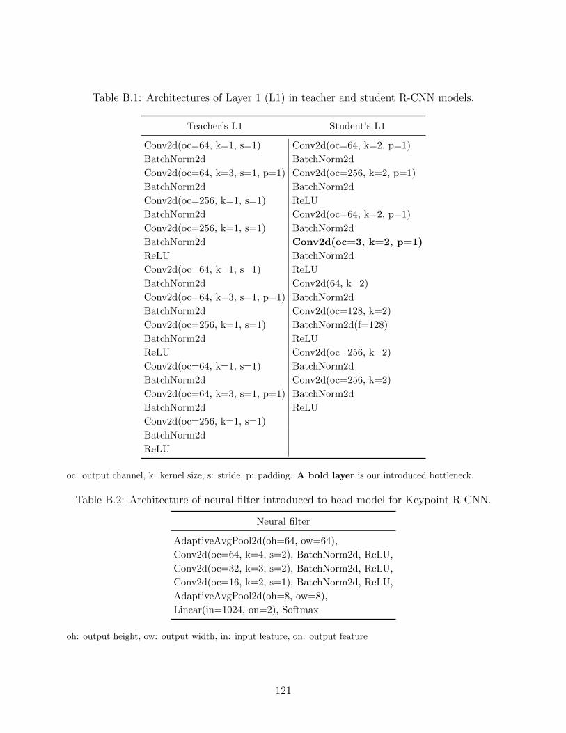
Table B.1: Architectures of Layer 1 (L1) in teacher and student R-CNN models.

Teacher’s L1 Student’s L1

Conv2d(oc=64, k=1, s=1) Conv2d(oc=64, k=2, p=1)

BatchNorm2d BatchNorm2d

Conv2d(oc=64, k=3, s=1, p=1) Conv2d(oc=256, k=2, p=1)

BatchNorm2d BatchNorm2d

Conv2d(oc=256, k=1, s=1) ReLU

BatchNorm2d Conv2d(oc=64, k=2, p=1)

Conv2d(oc=256, k=1, s=1) BatchNorm2d

BatchNorm2d Conv2d(oc=3, k=2, p=1)

ReLU BatchNorm2d

Conv2d(oc=64, k=1, s=1) ReLU

BatchNorm2d Conv2d(64, k=2)

Conv2d(oc=64, k=3, s=1, p=1) BatchNorm2d

BatchNorm2d Conv2d(oc=128, k=2)

Conv2d(oc=256, k=1, s=1) BatchNorm2d(f=128)

BatchNorm2d ReLU

ReLU Conv2d(oc=256, k=2)

Conv2d(oc=64, k=1, s=1) BatchNorm2d

BatchNorm2d Conv2d(oc=256, k=2)

Conv2d(oc=64, k=3, s=1, p=1) BatchNorm2d

BatchNorm2d ReLU

Conv2d(oc=256, k=1, s=1)

BatchNorm2d

ReLU

oc: output channel, k: kernel size, s: stride, p: padding. A bold layer is our introduced bottleneck.

Table B.2: Architecture of neural filter introduced to head model for Keypoint R-CNN.

Neural filter

AdaptiveAvgPool2d(oh=64, ow=64),

Conv2d(oc=64, k=4, s=2), BatchNorm2d, ReLU,

Conv2d(oc=32, k=3, s=2), BatchNorm2d, ReLU,

Conv2d(oc=16, k=2, s=1), BatchNorm2d, ReLU,

AdaptiveAvgPool2d(oh=8, ow=8),

Linear(in=1024, on=2), Softmax

oh: output height, ow: output width, in: input feature, on: output feature

121

Appendix C

- Chapter 5 -

C.1 Image Compression Codecs

As image compression baselines, we use JPEG, WebP [Google], and BPG [Bellard]. For

JPEG andWebP, we follow the implementations in Pillow1 and investigate the rate-distortion

(RD) tradeoff for the combination of the codec and pretrained downstream models by tuning

the quality parameter in range of 10 to 100. Since BPG is not available in Pillow, our

implementation follows [Bellard] and we tune the quality parameter in range of 0 to 50 to

observe the RD curve. We use the x265 encoder with 4:4:4 subsampling mode and 8-bit

depth for YCbCr color space, following [Begaint et al., 2020].

C.2 Quantization

This section briefly introduces the quantization technique used in both proposed methods

and neural baselines with entropy coding.

1https://python-pillow.org/

122

C.2.1 Encoder and Decoder Optimization

As entropy coding requires discrete symbols, we leverage the method that is firstly proposed

in [Balle et al., 2017] to learn a discrete latent variable. During the training stage, the

quantization is simulated with a uniform noise to enable gradient-based optimization:

z = fθ(x) + U(−1

2,1

2). (C.1)

During the inference session, we round the encoder output to the nearest integer for entropy

coding and the input of the decoder:

z = ⌊fθ(x)⌉. (C.2)

C.2.2 Prior Optimization

For entropy coding, a prior that can precisely fit the distribution of the latent variable reduces

the bitrate. However, the prior distributions such as Gaussian and Logistic distributions are

continuous, which is not directly compatible with discrete latent variables. Instead, we use

the cumulative of a continuous distribution to approximate the probability mass of a discrete

distribution [Balle et al., 2017]:

P (z) =

∫ z+ 12

z− 12

p(t)dt, (C.3)

where p is the prior distribution we choose, and P (z) is the corresponding probability mass

under the discrete distribution P . The integral can easily be computed with the Cumulative

Distribution Function (CDF) of the continuous distribution.

123

C.3 Neural Image Compression

In this section, we describe the experimental setup that we used for the neural image com-

pression baselines.

C.3.1 Network Architecture

Factorized prior model [Balle et al., 2018]. This model consists of 4 convolutional

layers for encoding and 4 deconvolutional layers for decoding. Each layer follows (128, 5, 2,

2) configuration in the format (number of channels, kernel size, stride, padding). We also

use the simplified version of generalized divisive normalization (GDN) and inversed GDN

(IGDN) [Balle et al., 2016] as activation functions for the encoder and decoder, respectively.

The prior distribution uses a univariate non-parametric density model, whose cumulative

distribution is parameterized by a neural network [Balle et al., 2018].

Mean-scale hyperprior model. We use exactly the same architecture described in [Min-

nen et al., 2018].

C.3.2 Training

All the models are trained on a high-resolution dataset with around 2,700 images collected

from DIV2K dataset [Agustsson and Timofte, 2017] and CLIC dataset [Toderici et al., 2020].

During training, we apply random crop size (256, 256) to the images and set the batch size as

8. We also use Adam [Kingma and Ba, 2015] optimizer with 10−4 learning rate to train the

model for 900,000 steps, and then the learning rate is decayed to 10−5 for another 100,000

steps.

124

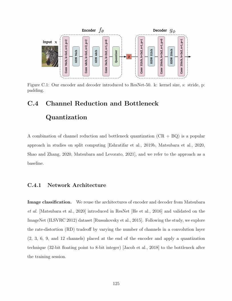
GDN

48c

h

GDN

96c

h

Conv

48c

h, k

=5x5

, s=2

, p=2

Conv

24c

h, k

=2x2

, s=1

, p=0

Conv

96c

h, k

=5x5

, s=2

, p=2

Quan

tize

r

Encoder Decoder

Conv

256

ch, k

=2x2

, s=1

, p=0

IGD

N 5

12ch

IGD

N 2

56ch

Conv

256

ch, k

=2x2

, s=1

, p=1

Conv

512

ch, k

=2x2

, s=1

, p=1Input

Figure C.1: Our encoder and decoder introduced to ResNet-50. k: kernel size, s: stride, p:padding.

C.4 Channel Reduction and Bottleneck

Quantization

A combination of channel reduction and bottleneck quantization (CR + BQ) is a popular

approach in studies on split computing [Eshratifar et al., 2019b, Matsubara et al., 2020,

Shao and Zhang, 2020, Matsubara and Levorato, 2021], and we refer to the approach as a

baseline.

C.4.1 Network Architecture

Image classification. We reuse the architectures of encoder and decoder from Matsubara

et al. [Matsubara et al., 2020] introduced in ResNet [He et al., 2016] and validated on the

ImageNet (ILSVRC 2012) dataset [Russakovsky et al., 2015]. Following the study, we explore

the rate-distortion (RD) tradeoff by varying the number of channels in a convolution layer

(2, 3, 6, 9, and 12 channels) placed at the end of the encoder and apply a quantization

technique (32-bit floating point to 8-bit integer) [Jacob et al., 2018] to the bottleneck after

the training session.

125

Object detection and semantic segmentation. Similarly, we reuse the encoder-decoder

architecture used as ResNet-based backbone in Faster R-CNN [Ren et al., 2015] and Mask

R-CNN [He et al., 2017a] for split computing [Matsubara and Levorato, 2021]. The same

ResNet-based backbone is used for RetinaNet [Lin et al., 2017b] and DeepLabv3 [Chen et al.,

2017c]. Again, we examine the RD tradeoff by controlling the number of channels in a bot-

tleneck layer (1, 2, 3, 6, and 9 channels) and apply the same post-training quantization

technique [Jacob et al., 2018] to the bottleneck.

C.4.2 Training

Using ResNet-50 [He et al., 2016] pretrained on the ImageNet dataset as a teacher model,

we train the encoder-decoder introduced to a copy of the teacher model, that is treated as

a student model for image classification. We apply the generalized head network distillation

(GHND) [Matsubara and Levorato, 2021] to the introduced encoder-decoder in the student

model. The model is trained on the ImageNet dataset to mimic the intermediate features

from the last three residual blocks in the teacher (ResNet-50) by minimizing the sum of

squared error losses. Using the Adam optimizer [Kingma and Ba, 2015], we train the student

model on the ImageNet dataset for 20 epochs with the training batch size of 32. The initial

learning rate is set to 10−3 and reduced by a factor of 10 at the end of the 5th, 10th, and

15th epochs.

Similarly, we use ResNet-50 models in RetinaNet with FPN and DeepLabv3 pretrained on

COCO 2017 dataset [Lin et al., 2014] as teachers, and apply the GHND to the students

for the same dataset. The training objective, the initial learning rate, and the number of

training epochs are the same as those for the classification task. We set the training batch

size to 2 and 8 for object detection and semantic segmentation tasks, respectively. The

learning rate is reduced by a factor of 10 at the end of the 5th and 15th epochs.

126

C.5 Proposed Student Model

This section presents the details of student models and training methods we propose in this

study.

C.5.1 Network Architecture

As illustrated in Fig. C.1, our encoder fθ is composed of convolution and GDN [Balle et al.,

2016] layers followed by a quantizer described in Section C.2. Similarly, our decoder gϕ is

designed with convolution and inversed GDN (IGDN) layers to have the output tensor shape

match that of the first residual block in ResNet-50 [He et al., 2016]. For image classification,

the entire architecture of our entropic student model consists of the encoder and decoder

followed by the last three residual blocks, average pooling, and fully-connected layers in

ResNet-50. For object detection and semantic segmentation, we replace ResNet-50 (used as

a backbone) in RetinaNet [Lin et al., 2017b] and DeepLabv3 [Chen et al., 2017c] with our

student model for image classification.

C.5.2 Two-stage Training

Here, we describe the two-stage method we proposed to train the entropic student models.

Image classification. Using the ImageNet dataset, we put our focus on the introduced

encoder and decoder at the first stage of training and then freeze the encoder to fine-tune all

the subsequent layers at the second stage for the target task. At the 1st stage, we train the

student model for 10 epochs to mimic the behavior of the first residual block in the teacher

model (pretrained ResNet-50) in a similar way to [Matsubara and Levorato, 2021] but with

the rate term to learn a prior for entropy coding. We use Adam optimizer with batch size of

127

64 and an initial learning rate of 10−3. The learning rate is decreased by a factor of 10 after

the end of the 5th and 8th epochs.

Once we finish the 1st stage, we fix the parameters of the encoder that has learnt compressed

features at the 1st stage and fine-tune all the other modules, including the decoder for the

target task. By freezing the encoder’s parameters, we can reuse the encoder for different

tasks. The rest of the layers can be optimized to adopt the compressible features for the

target task. Note that once the encoder is frozen, we also no longer optimize both the

prior and encoder, which means we can directly use rounding to quantize the latent variable.

With the encoder frozen, we apply a standard knowledge distillation technique [Hinton et al.,

2014] to achieve better model accuracy, and the concrete training objective is formulated as

follows:

L = α · Lcls(y,y) + (1− α) · τ 2 · LKL

(oS,oT

), (C.4)

where Lcls is a standard cross entropy. y indicates the model’s estimated class probabilities,

and y is the annotated object category. α and τ are both hyperparameters, and LKL is the

Kullback-Leibler divergence. oS and oT represent the softened output distributions from

student and teacher models, respectively. Specifically, oS = [oS1, oS2, . . . , o

S|C|] where C is a

set of object categories considered in target task. oSi indicates the student model’s softened

output value (scalar) for the i-th object category:

oSi =exp

(viτ

)∑k∈C exp

(vkτ

) , (C.5)

where τ is a hyperparameter defined in Eq. C.4 and called temperature. vi denotes a logit

value for the i-th object category. The same rules are applied to oT for teacher model.

For the 2nd stage, we use the stochastic gradient descent (SGD) optimizer with an initial

learning rate of 10−3, momentum of 0.9, and weight decay of 5×10−4. We reduce the learning

128

rate by a factor of 10 after the end of the 5th epoch, and the training batch size is set to

128. The balancing weight α and temperature τ for knowledge distillation are set to 0.5 and

1, respectively.

Object detection. We reuse the entropic student model trained on the ImageNet dataset

in place of ResNet-50 in RetinaNet [Lin et al., 2017b] and DeepLabv3 [Chen et al., 2017c]

(teacher models). Note that we freeze the parameters of the encoder trained on the ImageNet

dataset to make the encoder sharable for multiple tasks. Reusing the encoder trained on

the ImageNet dataset is a reasonable approach as 1) the ImageNet dataset contains a larger

number of training samples (approximately 10 times more) than those in the COCO 2017

dataset [Lin et al., 2014]; 2) models using an image classifier as their backbone frequently

reuse model weights trained on the ImageNet dataset [Ren et al., 2015, Lin et al., 2017b].

To adapt the encoder for object detection, we train the decoder for 3 epochs at the 1st stage

in the same way we train those for image classification (but with the encoder frozen). The

optimizer is Adam [Kingma and Ba, 2015], and the training batch size is 6. The initial

learning rate is set to 10−3 and reduced to 10−4 after the first 2 epochs. At the 2nd stage,

we fine-tune the whole model except its encoder for 2 epochs by the SGD optimizer with

learning rates of 10−3 and 10−4 for the 1st and 2nd epochs, respectively. We set the training

batch size to 6 and follow the training objective in [Lin et al., 2017b], which is a combination

of L1 loss for bounding box regression and Focal loss for object classification.

Semantic segmentation. For semantic segmentation, we train DeepLabv3 in a similar

way. At the 1st stage, we freeze the encoder and train the decoder for 5 epochs, using

Adam optimizer with batch size of 8. The initial learning rate is 10−3 and decreased to 10−4

after the first 3 epochs. At the 2nd stage, we train the entire model except for its encoder

for 5 epochs. We minimize a standard cross entropy loss, using the SGD optimizer. The

129

initial learning rates for the body and the sub-branch (auxiliary module)2 are 2.5×10−3 and

2.5 × 10−2, respectively. Following [Chen et al., 2017c], we reduce the learning rate after

each iteration as follows:

lr = lr0 ×(1− Niter

Nmax iter

)0.9

, (C.6)

where lr0 is the initial learning rate. Niter and Nmax iter indicate the accumulated number of

iterations and the total number of iterations, respectively.

C.5.3 End-to-end Training

In this work, the end-to-end training approach for feature compression [Singh et al., 2020] is

treated as a baseline and applied to our entropic student model without teacher models.

Image classification. Following the end-to-end training approach [Singh et al., 2020], we

train our entropic student model from scratch. Specifically, we use Adam [Kingma and Ba,

2015] optimizer and cosine decay learning rate schedule [Loshchilov and Hutter, 2017] with

an initial learning rate of 10−3 and weight decay of 10−4. Based on their training objectives

(Eq. C.7), we train the model for 60 epochs with batch size of 256.3 Note that Singh et

al. [Singh et al., 2020] evaluate the accuracy of their models on a 299 × 299 center crop.

Since the pretrained ResNet-50 expects the crop size of 224× 224,4 we use the crop size for

all the considered classifiers to highlight the effectiveness of our approach.

2https://github.com/pytorch/vision/tree/master/references/segmentation3For the ImageNet dataset, Singh et al. train their models for 300k steps with batch size of 256 for 1.28M

training samples, which is equivalent to 60 epochs (= 300k×2561.28M ).

4https://pytorch.org/vision/stable/models.html#classification

130

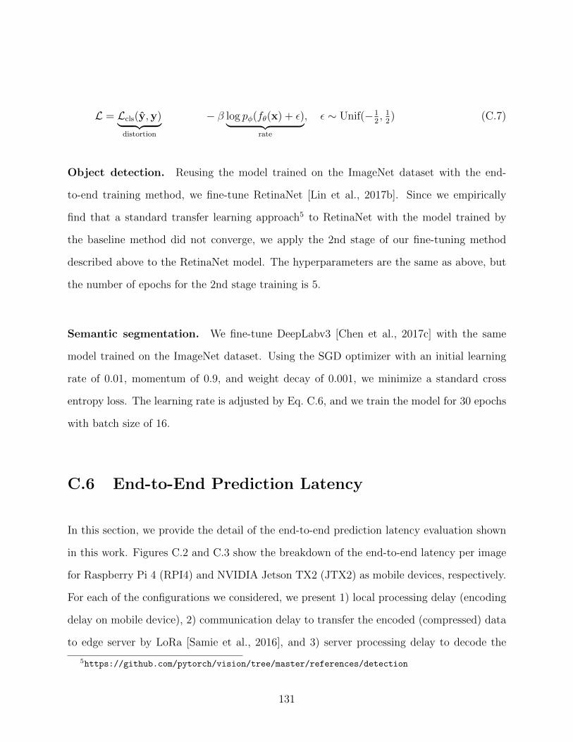
L = Lcls(y,y)︸ ︷︷ ︸distortion

− β log pϕ(fθ(x) + ϵ)︸ ︷︷ ︸rate

, ϵ ∼ Unif(−12, 12) (C.7)

Object detection. Reusing the model trained on the ImageNet dataset with the end-

to-end training method, we fine-tune RetinaNet [Lin et al., 2017b]. Since we empirically

find that a standard transfer learning approach5 to RetinaNet with the model trained by

the baseline method did not converge, we apply the 2nd stage of our fine-tuning method

described above to the RetinaNet model. The hyperparameters are the same as above, but

the number of epochs for the 2nd stage training is 5.

Semantic segmentation. We fine-tune DeepLabv3 [Chen et al., 2017c] with the same

model trained on the ImageNet dataset. Using the SGD optimizer with an initial learning

rate of 0.01, momentum of 0.9, and weight decay of 0.001, we minimize a standard cross

entropy loss. The learning rate is adjusted by Eq. C.6, and we train the model for 30 epochs

with batch size of 16.

C.6 End-to-End Prediction Latency

In this section, we provide the detail of the end-to-end prediction latency evaluation shown

in this work. Figures C.2 and C.3 show the breakdown of the end-to-end latency per image

for Raspberry Pi 4 (RPI4) and NVIDIA Jetson TX2 (JTX2) as mobile devices, respectively.

For each of the configurations we considered, we present 1) local processing delay (encoding

delay on mobile device), 2) communication delay to transfer the encoded (compressed) data

to edge server by LoRa [Samie et al., 2016], and 3) server processing delay to decode the

5https://github.com/pytorch/vision/tree/master/references/detection

131

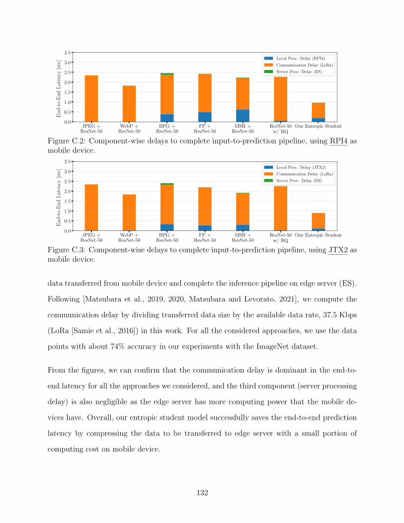
JPEG +ResNet-50

WebP +ResNet-50

BPG +ResNet-50

FP +ResNet-50

MSH +ResNet-50

ResNet-50w/ BQ

Our Entropic Student0.0

0.5

1.0

1.5

2.0

2.5

3.0

3.5End-to-EndLatency

[sec] Local Proc. Delay (RPI4)

Communication Delay (LoRa)

Server Proc. Delay (ES)

Figure C.2: Component-wise delays to complete input-to-prediction pipeline, using RPI4 asmobile device.

JPEG +ResNet-50

WebP +ResNet-50

BPG +ResNet-50

FP +ResNet-50

MSH +ResNet-50

ResNet-50w/ BQ

Our Entropic Student0.0

0.5

1.0

1.5

2.0

2.5

3.0

3.5

End-to-EndLatency

[sec] Local Proc. Delay (JTX2)

Communication Delay (LoRa)

Server Proc. Delay (ES)

Figure C.3: Component-wise delays to complete input-to-prediction pipeline, using JTX2 asmobile device.

data transferred from mobile device and complete the inference pipeline on edge server (ES).

Following [Matsubara et al., 2019, 2020, Matsubara and Levorato, 2021], we compute the

communication delay by dividing transferred data size by the available data rate, 37.5 Kbps

(LoRa [Samie et al., 2016]) in this work. For all the considered approaches, we use the data

points with about 74% accuracy in our experiments with the ImageNet dataset.

From the figures, we can confirm that the communication delay is dominant in the end-to-

end latency for all the approaches we considered, and the third component (server processing

delay) is also negligible as the edge server has more computing power that the mobile de-

vices have. Overall, our entropic student model successfully saves the end-to-end prediction

latency by compressing the data to be transferred to edge server with a small portion of

computing cost on mobile device.

132