IN DEGREE PROJECT COMPUTER SCIENCE AND ENGINEERING,SECOND CYCLE, 30 CREDITS

, STOCKHOLM SWEDEN 2019

Movement trajectory classification using supervised machine learning

ALEX TEATINI

KTH ROYAL INSTITUTE OF TECHNOLOGYSCHOOL OF ELECTRICAL ENGINEERING AND COMPUTER SCIENCE

Movement trajectory classification using supervised machine learning

ALEX TEATINI

Master’s degree in ICT Innovation (TIVNM) Digital Media Technology track (DMTE) Supervisor: Erik Fransén Examiner: Pawel Herman Swedish Title: Klassificering av rörelsebana med övervakad maskininlärning School of Electrical Engineering and Computer Science

Abstract

  Anything that moves can be tracked, and hence its trajectory analysed. The                       trajectory of a moving object can carry a lot of useful information                       depending on what is sought. In this work, the aim is to exploit machine                           learning to be able to classify finite trajectories based on their shape. In a                           clinical environment, a set of trajectory classes have been defined based on                       relevance to particular pathologies. Furthermore, several trajectories have               been collected using a depth sensor from a number of subjects. The                       problem to address is to evaluate whether it is possible to classify these                         trajectories into predefined classes. 

A trajectory consists of a sequentially ordered list of coordinates, which                     would imply temporal processing. However, following the success of                 machine learning to classify images, the idea of a visual approach surfaced.                       On this basis, the plots of the trajectories are transformed into images,                       making the problem become similar to a written character recognition                   problem. The implemented methods for this classification tasks are the                   well-known Support Vector Machine (SVM) and the Convolutional Neural                 Network (CNN), the most appreciated deep approach to image recognition.                   We find that the best possible way to of achieving substantial performances                       on this classification task is to use a mixture of the two aforementioned                         methods, namely a two-step classification made of a binary SVM,                   responsible for a first distinction, followed by a CNN for the final decision.                         We illustrate that this tree-based approach is capable of granting the best                       classification accuracy score under the imposed restrictions.  

In conclusion, a look into possible future developments based on the                     exploration of novel deep learning methods will be given. This project has                       been developed during an internship at the company ‘Qinematic’.    

 

Sammanfattning

Allt som rör sig kan detekteras och därmed kan dess bana

analyseras. Banan för ett rörligt objekt kan bära en hel del användbar information beroende på vad som eftersöks. I detta arbete är syftet att utnyttja maskininlärning för att kunna klassificera ändliga banor baserat på deras form. I en klinisk miljö har en uppsättning banklasser definierats baserat på dess relevans för vissa sjukdomar. Vidare har flera banor samlats in med hjälp av en djupledssensor från ett antal personer. Projektets syfte är att utvärdera om det är möjligt att klassificera dessa banor i de fördefinierade klasserna.

En bana består av en sekventiellt ordnad lista av koordinater, vilket skulle antyda temporal behandling. Men utifrån framgången av maskininlärning för att klassificera bilder fick vi idén om en bildbaserad analys. På grundval av detta har banor omvandlas till bilder, vilket gör att problemet nu liknar igenkänningsproblemet av handskrivna siffror. De genomförda metoderna för klassificeringsuppgiften är den välkända Support Vector Machine (SVM), implementerad i några olika konfigurationer samt Convolutional Neural Network (CNN), den mest uppskattade metoden för bildigenkänning inom Deep Learning. Vi finner att bästa möjliga sätt för att uppnå betydande prestationer på klassificeringsuppgiften är att använda en blandning av de två tidigare nämnda metoderna, nämligen en tvåstegsklassificering gjord av en binär SVM, ansvarig för en första distinktion, följt av en CNN för det slutliga beslutet. Vi visar att detta trädbaserade tillvägagångssätt kan ge den bästa klassnoggrannheten under ålagda restriktioner.

Avslutningsvis ges en hypotes för framtida förbättringar av nya djupa inlärningsmetoder.

Table of Contents

1 Introduction 1 

1.1 Problem 2 

1.2 Limitations 2 

1.3 Purpose 3 

 

2 Background 4 

2.1 Related work on trajectory analysis 4 

2.2 The MNIST database and character recognition 5 

2.3 Other visual approaches 6 

2.4 Machine learning methods overview 6  2.4.1 Support Vector Machine 7  2.4.2 Convolutional Neural Network 8 

 

3 Methods 9 

3.1 Description of the data and pre-processing 9 

3.2 The implemented methods 10  3.2.1 Multiclass SVM 11  3.2.2 SVM cascade 11  3.2.3 SVM tree 13  3.2.4 Convolutional Neural Network 14 

3.3 Pilot work to adapt to the problem 14 

3.4 Evaluation metrics 15 

 

4 Results 16 

4.1 Multiclass SVM 16 

4.2 SVM cascade and SVM tree 17 

4.3 Convolutional Neural Network 17 

4.4 Mixture of SVM and CNN 18 

 

 

5 Discussion and future work 21 

5.1 Discussion on multiclass classification 21 

5.2 Discussion on macro-class grouping results 21 

5.3 Comparison to related work 22 

5.4 Notable outcomes 23  5.4.1 SVM and CNN work well together 23  5.4.2 Advantages of a visual perspective 23  5.4.3 Data bounded performance 23 

5.5 Future work: One-Shot Learning 24 

5.6 Ethic and sustainability 25 

 

6 Conclusions 26  

References 27  

Appendix 30   

 

 

1

Chapter 1

Introduction When any kind of object moves, it can be followed by the human eye,

or tracked by a sensor, in order to see and analyse its movement trajectory [1], [2]. A set of points representing the position in space of a moving object at consecutive instants is called trajectory [3]. A generic example for a two-dimensional trajectory of a moving object described with a plot is shown in Figure 1.1.

Figure 1.1: Example of a random two-dimensional trajectory of a generic object moving in space. The axes represent the coordinates in space (measured in meters) and the line

(trajectory) is the path of the moving object. The plot has no specific meaning and is for demonstration purposes only.

Space [m]

Space [m]

2

There is a lot of useful information that can be obtained by observing the trajectory of something that moves, be it a human being, an animal, a vehicle or any other kind of thing. In fact, analysis of trajectories of moving objects has always been a task of considerable importance. Nowadays, machine learning has a fundamental role in many automatic recognition problems, and thus also in trajectory analysis [4], [5], [6].

1.1 Problem In this project, a movement trajectory classification problem has

been treated and addressed using machine learning. Movement trajectories can be analysed under various points of view and with several purposes. Different kind of approaches can be unsupervised clustering or supervised analysis. Furthermore, the perspective can be two-dimensional or three-dimensional, and aspects to consider can be kinetic information (velocity, acceleration) or only coordinates.

The main research question in this work is how well some specific machine learning methods can classify two-dimensional movement trajectories into pre-defined patterns (movement classes), without taking into account the kinetic information. Based on the results achieved in previous work [16], [17], [19], [20], it is explored how well widely used methods such as SVM and CNN perform on the given task. Furthermore, it is tested how a hybrid architecture of the two aforementioned methods is able to perform in comparison to the two separate methods and if it can lead to better results.

1.2 Limitations Generally speaking, trajectory classification can be seen under two

different perspectives. On one side there is a data-driven approach, which aims to perform clustering of the trajectories in order to group similar ones and detect outliers. However, in this way, the results are data dependent, and a trend in the data is not necessarily what is sought. On the other side, the goal is to assign trajectories to predefined classes, which is the case of this project. The biggest challenges for this kind of task are to be able to process the data adequately and to understand which are the methods that allow reaching the desired goals under the named restrictions.

Another major limitation is given by the fact that the available data was unlabelled. It was necessary to look at every sample with the supervision of an expert and to manually assign one of the searched

3

classes to each one of them. However, a human decision introduces a bias, especially in some borderline or heavily noisy cases, where no evident class can be assigned with total certainty.

1.3 Purpose

There are several motivations to work on trajectory analysis of every

kind. It can be useful for detecting outliers, recognizing recurrent patterns or categorizing movements. Regarding this particular work, the focus is set on being able to recognize and/or categorize movement trajectories according to specific patterns. This can be useful in many different fields. In sports, for example, it could be interesting to recognize a particular style of movement by looking at the trajectory of a sportsman, e.g. in winter sports. Another use of such a technology could be found in evaluating an anatomical body analysis, in order to detect possible diseases or injuries. No to be forgotten, even the observation of movement patterns of wild animals or vehicles are very interesting tasks that could use the information provided by automatic analysis.

4

Chapter 2

Background

2.1 Related work on trajectory analysis

Trajectory analysis has been treated in multiple ways and in

different contexts throughout literature. In most cases, the goal of trajectory analysis was to detect outliers or to predict future states using data-driven machine learning approaches. Fewer have been the approaches under a static point of view instead.

Li et al. [7] used a rule-based classifier to do hierarchical feature classification. In their work, they presented a technique for anomaly detection of moving objects called ROAM. In their research, trajectories are expressed as a set of discrete fragments called motifs, which form a multidimensional feature space for every sample. A rule-based classifier is then responsible for a hierarchical exploration of the feature space to find the effective regions which define an anomaly. Likewise, Lee et al. [8] presented an outlier detection algorithm based on the partitioning of the trajectory. The concept is similar to the previously cited work, with the difference that in this case, the aim is to detect also outlier sub-trajectories. Here the detection is done with a hybrid of a distance- and a density-based approach. Another work by the same authors [9] presented a method for trajectory clustering based on the same principles of sub-trajectories. A further clustering approach is the one presented by Holst and Jonasson [10] in their paper about movement classification in skiing. In this work the data is modelled using a Markov chain of multivariate Gaussian distributions and classification is then performed based on that. The intention was to classify and detect different cross-country skiing techniques called gears. In this case, the analysed data proceeds from an accelerometer placed on the skier. Similarly, Bashir et al. [11] presented a method for recognizing object activities based on their motion trajectories using Gaussian mixture models with the help of hidden Markov models to preserve temporal relations. Here too the approach is data-driven. Sas et al. [12] addressed

5

a trajectory clustering problem using artificial neural networks. In their work for online trajectory classification, they propose a modular system to cluster trajectories deriving from navigation in virtual environments.

Vehicle trajectory and traffic analysis is also a task of high interest, especially for its real-life applications. Kumaran et al. [13] presented work on anomaly detection and trajectory classification on traffic surveillance videos. By using a hybrid Convolutional Neural Network and Variational Autoencoder they were able to detect outliers and classify trajectories with impressive accuracy. Khosroshahi et al. [14] presented work related to vehicle trajectory analysis as well. In particular, they performed behaviour analysis of surrounding vehicles for autonomous driving using Recurrent Neural Networks. Their aim was to classify the type of manoeuvres of other vehicles with a Long Short Term Memory model using their trajectories.

2.2 The MNIST database and character recognition Up to this point, the quoted researches do not look at the trajectory

classification problem in the same way it has been done in this work. Looking at a finite trajectory in order to recognize a known pattern is in a remote way analogous to a character recognition problem. The literature in the area of image classification and computer vision for character recognition is full of researches and publications. Most of them are somehow related to the MNIST database of handwritten digits published by LeCun et al. [15]. The MNIST database contains 70000 images of handwritten digits (from 0 to 9) drawn in black on a white background. It is for sure the most used dataset exploited to train plenty of different machine and deep learning models for character recognition tasks. LeCun himself has experimented with plenty of different algorithms for classification on the aforementioned dataset [16]. He reported performances of methods like Nearest Neighbours (k-NN), Support Vector Machine and artificial neural networks for character recognition. Furthermore, his publication describes a gradient-based learning method, called Graph Transformer Network, successfully applied to document recognition. Belongie et al. [17] presented a method with the scope of shape matching based on a k-NN classifier. In their work, they obtain accurate results on the MNIST database. Simard et al. [18] describe how to best use neural networks for visual document analysis. They underline the importance of a large dataset and prove the superiority of convolutional networks over fully connected architectures for the mentioned task. Cireşan et al. [19] claim one of the best classification accuracies on the MNIST database, namely 99.65%. They

6

stand on the fact that a simple multi-layer perceptron with back-propagation with many hidden layers, many neurons and high computational power is enough to achieve outstanding results. 2.3 Other visual approaches

There are only a few relevant examples in the literature where a

visual recognition approach, different from character recognition, was taken for trajectory classification tasks. Hse and Newton [20] presented a work whose purpose was to recognize sketched symbols that are not proper characters. These sketched symbols could be geometric figures or small drawings. Hse and Newton used Zernike moments to describe the data and applied different classification algorithms such as Support Vector Machine, Nearest Neighbours and Minimum Mean Distance. They found out that SVM was the most accurate method for their task.

Differently, Wang and Oates [21] tried to encode time series data as images for classification purposes. Time series were encoded as different kinds of images, namely Gramian Angular Fields and Markov Transition Fields, in order to be able to apply computer vision techniques on them. Titled Convolutional Neural Networks were then implemented for classification obtaining remarkable results. The approach which is described in this research leverages on the same concept of image encoding.

2.4 Machine learning methods overview In order to have preventive knowledge about the main concepts of

machine learning, an essential overview of the methods presented in this thesis will be given first. The chosen algorithms are the Support Vector Machine and the Convolutional Neural Network.

Generally speaking, for a machine learning kind of problem the data to process has to be split into two subsets: training and test set. Like the names says, the training of the model is done on the training set, while the evaluation is then done on the test set. In order to get a more veritable evaluation of the average performance of the model, it is often common to shuffle the data, split it and then train the model for a given number of times. During the training phase, a smaller part of the training set, called validation set, is cut off and used as a preventive test set to validate the model accuracy. This process is normally done N times and is called N-fold cross-validation. Usually, a machine learning model has some hyperparameters which have to be set. A common way

7

to automatically tune these parameters is by using a method called Grid search, in which the optimal values are determined for a given model during the process of cross-validation.

2.4.1 Support Vector Machine One approach that has been chosen for implementation is one of the

most known and widely used machine learning algorithms, which is the Support Vector Machine, in short SVM. The main idea of the SVM is to map the data into a higher dimensional space by using a so-called kernel function and to find the hyperplane which best divides the data into the desired classes. The ones which are called support vectors are the data points which are nearest to the hyperplane and are thus used to make the decision. To illustrate the idea, figure 2.1 shows an example of some generic data points divided by the hyperplane and the corresponding support vectors. The following equations show some possible examples of kernel functions that can be applied to the data. Specifically, we show the Radial Basis Function kernel as

!"#$%&', &)* = -./%01.02*3,

where the inputs are two data points and 4 is the kernels hyperparameter, and the polynomial kernel as

!5678%&', &)* = %&' ⋅ &) + ;*

<,

where d is the polynomials degree and c the free coefficient.

8

Figure 2.1: Example of a hyperplane with its relative support vectors separating some

generic data points. The orange and blue dots represent the data from two different classes, where the circled ones are the data points used as support vectors. The continuous line is the

separation hyperplane, while the dashed lines are delimiting the decision boundary dictated by the support vectors. On the axes, the values of the features of the data are represented, which have some generic unit. This figures purpose is purely demonstrative. The images' source is

[26].

2.4.2 Convolutional Neural Network The idea of a neural network was inspired by the deep learning

architectures used on the MNIST database available in the literature. A Convolutional Neural Network, or CNN, is a particular type of Neural Network often used for image classification purposes. As the name suggests, it is based on convolutional operations on two-dimensional data. These operations happen in the so-called convolutional layers of the network and have the purpose of extracting relevant features from the data. The other kind of layer which is normally present in a CNN is the max-pooling layer, which appears between convolutional layers. The classification is performed in the last layer of the network, which normally is a so-called SoftMax function.

9

Chapter 3

Methods

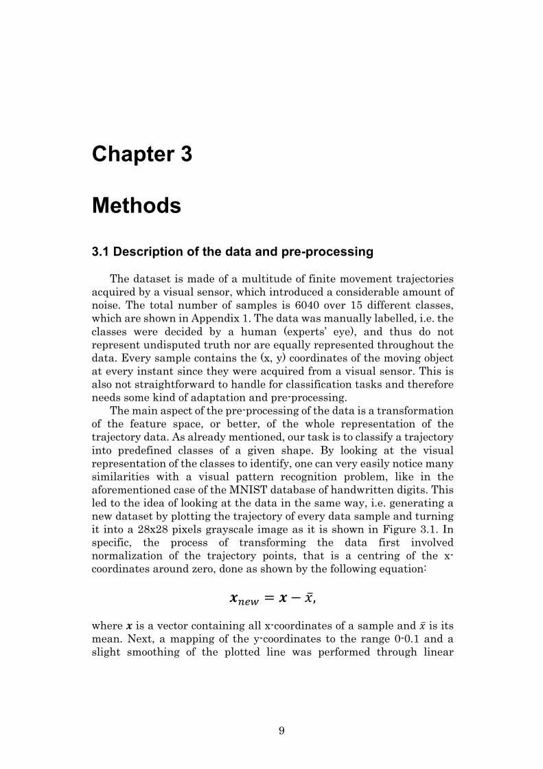
3.1 Description of the data and pre-processing The dataset is made of a multitude of finite movement trajectories

acquired by a visual sensor, which introduced a considerable amount of noise. The total number of samples is 6040 over 15 different classes, which are shown in Appendix 1. The data was manually labelled, i.e. the classes were decided by a human (experts’ eye), and thus do not represent undisputed truth nor are equally represented throughout the data. Every sample contains the (x, y) coordinates of the moving object at every instant since they were acquired from a visual sensor. This is also not straightforward to handle for classification tasks and therefore needs some kind of adaptation and pre-processing.

The main aspect of the pre-processing of the data is a transformation of the feature space, or better, of the whole representation of the trajectory data. As already mentioned, our task is to classify a trajectory into predefined classes of a given shape. By looking at the visual representation of the classes to identify, one can very easily notice many similarities with a visual pattern recognition problem, like in the aforementioned case of the MNIST database of handwritten digits. This led to the idea of looking at the data in the same way, i.e. generating a new dataset by plotting the trajectory of every data sample and turning it into a 28x28 pixels grayscale image as it is shown in Figure 3.1. In specific, the process of transforming the data first involved normalization of the trajectory points, that is a centring of the x-coordinates around zero, done as shown by the following equation:

=>?@ = = − &̅,

where = is a vector containing all x-coordinates of a sample and &̅ is its mean. Next, a mapping of the y-coordinates to the range 0-0.1 and a slight smoothing of the plotted line was performed through linear

10

interpolation. At this point, the points were plotted and the figures containing the plots saved as new images in PNG format, which then became the new dataset. The training set was obtained from 80% of the dataset, while the remaining 20% became the test set.

Figure 3.1: A trajectory (black line) of the dataset encoded as a 28x28 pixels grayscale image. These 28x28 pixels images are the new handled data. The axes show the size in pixels

(28x28) of the image.

3.2 The implemented methods

In this subsection, a more detailed explanation of how the methods

have been used and the related steps and choices will be given. Following a logical order, the first method illustrated is the already mentioned Support Vector Machine, applied for a 15-class classification task. A model deriving from the multiclass SVM referred to as SVM cascade will follow. After that, some major changes in the classes to be detected will be illustrated, before talking about an SVM-based tree model. In the last subsection, the deep learning approach, namely the Convolutional Neural Network, will be treated.

Pixel

Pixel

11

3.2.1 Multiclass SVM

Among many similar methods, the Support Vector Machine was

chosen for its versatility and the good results it can obtain on character recognition tasks, as it did in [15]. The multiclass SVM was implemented using the Scikit Learn libraries for the programming language Python [22]. For the 15-class classification task an SVM with RBF kernel function was chosen and its main parameters, which are the regularization parameter C and the free parameter of the kernel function g (gamma), have been tuned through Grid search during a 3-fold cross-validation process. The RBF kernel was selected over other types of kernel functions since it is widely used for multiclass classification problems. To solve the problem of multiple classes that needed to be classified, a “one-vs-one” approach was chosen in order to better define boundaries between similar classes at cost of higher computational needs (this applies also to all future multi-class SVM cases).

3.2.2 SVM cascade Generally, the output of an SVM can be either the predicted class or

a vector of probabilities, containing the probabilities of the analysed sample belonging to each class. Due to the high similarity between some classes, it could be assumed that if an error using a standard SVM occurred, the correct class would still be one of the most probable ones, i.e. one of the next possible choices. Based on this idea the concept of a cascade of several SVMs was founded. This model implies to perform three predictions one after the other. The first of the three predictions was done by the same 15-class model which was used in the first approach, whose output, however, was changed to the probabilities for each class. It had been empirically determined that the correct class is between the 6 most probable classes with a 95% confidence. Hence, the second prediction was done by training an additional 6-class SVM with the same parameters as the first one with the same kind of probabilistic output. At this point, the last prediction was performed with a binary SVM to distinguish between the 2 most probable classes. A set of binary SVMs was pre-trained for every possible combination of 2 classes and the parameters of every SVM were tuned through Grid search in a 2-fold cross-validation. A visual scheme of the cascade of SVMs is shown in Figure 3.2.

12

Figure 3.2: Scheme of the SVM cascade. The vector X contains one input sample. The

vectors P(y) contain the relative class probabilities after each prediction and CDis the predicted class.

After evaluating the performances of the just illustrated methods, it

became clear that the difficulties introduced by the data itself make it considerably hard to achieve good classification results. As already mentioned, the data is hand-labelled, and the defined classes are thus in some way biased by the humans' decision. Furthermore, some classes are very similar to each other and other ones are very poorly represented, both visually and numerically. Therefore, it had been decided to simplify the task by making some changes to the data and the expected outcome. By dropping a grouping some of the 15 classes, new “macro-classes” were defined and taken as the target from this point onwards. The changes to the classes are shown in Figure 3.3 and the number of samples of the dataset became 5084 over 5 classes.

Figure 3.3: Grouping of the 15 classes into 5 macro-classes. Notice that C8 and C9 are

mapped into “None”, which means the classes are dropped.

None

13

3.2.3 SVM tree

From the same principle of the SVM cascade, which focuses on a

stepwise analysis, the idea of the following approach sprang out. This approach towards the newly defined macro-classes is another type of stepwise classification, relying on a model which can be referred to as SVM tree. The idea is trivial and has only two steps. In the first one, there is a binary distinction between class 1 and all the others, followed by a 4-class classification in case the first decision would not have been for class 1. Since class 1 represents a straight line while the other classes show some kind of curve, it can be assumed that making this prior distinction could result in better overall accuracy. A scheme showing the ideated model is shown in Figure 3.4. For the binary classification, an SVM with a polynomial kernel of degree 7 had been implemented, because a polynomial kernel is better suited for binary classification. The degree of the polynomial had been tuned with a Grid search process. For the macro-class distinction, an SVM with RBF kernel had been chosen. Here too the parameters were tuned using Grid search within the cross-validation, splitting the data 3 times.

Figure 3.4: Scheme of the SVM tree. The vector X contains one input sample. The first

prediction is given by CD′, while CD is the final prediction.

14

3.2.4 Convolutional Neural Network Due to the great performances on the MNIST database [15] and in

image classification tasks in general [23], it seemed appropriate to implement also a deep learning approach by training a Convolutional Neural Network. The CNN was trained with for the direct 5-class classification and was implemented in Python using the Keras framework with a TensorFlow backend [24] and the architecture of the network can be seen in Figure 3.5. Like in the cases before, 3-fold cross-validation has been applied and the network was trained for 50 epochs.

Figure 3.5: 5-class CNN architecture.

3.3 Pilot work to adapt to the problem

For the last method, a mixture of the two previous models has been built. This has been done under the assumption that the SVM is more accurate than the CNN when it comes to a binary distinction, while the CNN performs better on multiple classes. Thus, a tree-based combination of SVM and CNN has been implemented to adapt to the problem. Like in the case of the SVM tree, an input sample is first passed to a binary SVM. In the case where the output class would be different from 1, the 4-class distinction is performed by a 4-class CNN, trained to distinguish the aforementioned macro-classes. The networks architecture can be seen in Figure 3.6. The cross-validation was done on 3 folds and the network was trained for 30 epochs, as it had been found out previously that more epochs would lead to overfitting.

15

Figure 3.6: 4-class CNN architecture.

3.4 Evaluation metrics Since we have a direct classification problem where every processed

sample gets the predicted label assigned and no class is more important than others, the performances were evaluated using a simple classification accuracy score measured as

F;; =

GHIJK?LI?MI

,

where GHIJK? is the number of correct classifications and N the total number of test samples. The accuracy score is measured as a percentage value. The same is true for the accuracy score measured on the validation set.

For the evaluation of the CNN the same kind of metrics, i.e. accuracy score, has been used. Additionally, a categorical cross-entropy loss function is taken into consideration. These two values are measured after every epoch on the validation set and for the final evaluation on the test set.

To have a closer look at the classification outcome, it is common to refer to the so-called confusion matrix. This particular matrix shows all matches and errors on the test set. The number of correctly classified samples for each class are shown on the diagonal of the matrix, while in the other slots the wrongly classified samples are situated. This can be useful to see which classes are more difficult to classify or distinguish, i.e. where more errors occur.

16

Chapter 4

Results

4.1 Multiclass SVM

The first relevant results are those relative to the standard 15-class

SVM, before grouping some classes together. During the classification, every test sample has been assigned to one of the 15 classes. The best parameters obtained with the grid search were C = 100 and g = 0.01, which lead to a validation accuracy of 56%. Even though a lot of work and effort have been invested in finding the best configuration for the applied multiclass SVM, the resulting test accuracy score was just ~57%. The confusion matrix relative to the multiclass SVM testing is shown in Table 4.1. From the confusion matrix, it can be observed how many matches were hit for each class. Those matches are shown in the green cells. Additionally, it can be useful to observe what misclassification errors happen more commonly, for example by observing that class 6 can easily be mistaken for class 13. Thus, it can also be observed which classes are more difficult to handle.

Table 4.1: Multiclass SVM confusion matrix. The values on the diagonal marked in green show

the correct classifications, while the rest of the values are wrong classifications.

17

4.2 SVM cascade and SVM tree The idea to put several SVMs in cascade relying on the class

probabilities had the purpose to improve the outcome of a standard SVM implementation. The measured average test accuracy of the method referred to as SVM cascade was ~55% though, which is even 1% lower than the standard SVM implementation. This could possibly be because, even if it seemed logically plausible that this approach would turn out to be able to classify the data more accurately, the problems related to the data itself did not make it possible to improve in this way. More to this can be found in the Discussion section.

The following concept of the SVM tree to distinguish between the bigger macro-classes after grouping similar classes with each other turned out to be able to grant some important improvements. From the parameter tuning process done with a grid search technique, the following results emerged. The best parameters for binary classification were C = 1000 and g = 0.001 with a validation accuracy of 94%. The best parameters for macro classification instead were C = 10 and g = 0.01 with a validation accuracy score of 82%. The overall average accuracy obtained on the test set was ~79% and the relative confusion matrix is shown in Table 4.2.

Table 4.2: SVM tree confusion matrix. The values on the diagonal show the correct

classifications. It can be seen that most errors occur in classes 2-5.

4.3 Convolutional Neural Network Coming to the second kind of approach, the Convolutional Neural

Network was built with the same purpose of distinguishing the 5 macro classes described above. It was trained for 50 epochs with a 3-fold cross-validation process, where the validation set was obtained by randomly cutting off a subset of 10% of the training set at every iteration. Note that the models’ weights were saved after every epoch, in order to be

18

able to restore them whenever needed. Both training and validation accuracy and loss were measured after every epoch and can be seen in a graph in Figure 4.1. The blue plot represents the metrics relative to the training and the orange one the metrics relative to the validation. As we can notice by looking at the curve trend, the model slowly overfits after 30-35 epochs. When the training was over, the weights deriving from the training epoch with the highest validation accuracy were restored and used to test the model. After evaluation, the resulting average test accuracy and loss are reciprocally ~79% and 0.74.

Figure 4.1: Accuracy (upper panel) and loss (lower panel) versus number of epochs for

training (blue) and validation set (orange). These plots are relative to the training of the 5-class CNN.

4.4 Mixture of SVM and CNN The last implemented model, which turned out to be also the best

model tested within this project, is the binary SVM followed by a 4-class CNN. Since the binary SVM is the same that was used in the case of the

19

SVM tree, its parameters are also the same, i.e. a polynomial kernel function of degree 7 with C = 1000 and g = 0.001 with a validation accuracy score of ~94%. The 4-class CNN was trained for 30 epochs as opposed to the 5-class CNN which was trained for 50 epochs, and in Figure 4.2 the plots showing accuracy and loss against the number of epochs are presented. From the plots, we can notice how the trend of both curves has a desirable look according to standard evaluations on neural network training. From the final evaluation on the test set an overall average accuracy of ~84% was obtained and its relative confusion matrix is shown in Table 4.3.

Finally, Table 4.4 shows a brief summary of the obtained results pointing out the best performance. As already mentioned, the combination of binary SVM and 4-class CNN appeared to be the best performing method among the implemented ones.

Table 4.3: Mixed Model confusion matrix. The correct classifications are shown on the

diagonal marked in green. Slight improvements can be noticed in comparison to table 4.2.

Table 4.4: Resume of the obtained results for all implemented methods. It can be seen that the highest test accuracy was obtained from the Mixed Model.

20

Figure 4.2: Accuracy (upper panel) and loss (lower panel) versus number of epochs for

training (blue) and validation set (orange) relative to the training of the 4-class CNN part of the mixture model.

21

Chapter 5

Discussion and future work In this section, the obtained results will be analysed and discussed.

Comparison based on classification accuracy will be given, and after that, the idea of a possible future approach will be treated. It has to be noted that unfortunately there is no statistical evidence of the results to be reported. Due to time constraints, it was not possible to collect multiple runs of the experiments, and thus to do statistical testing. For this reason, the discussion and the conclusions deriving from it are suggestive rather than conclusive. This should be kept in mind for everything that follows.

5.1 Discussion on multiclass classification Due to the noisy, unbalanced and manually labelled dataset, the

average accuracy obtained from the testing of the multiclass SVM implemented in a multitude of different configuration and with several different parameters, turned out to be only ~57% at best, as you have seen in the previous section. The expectations for a powerful method such as SVM for classification problems were definitely higher. Furthermore, the hypothesis of obtaining better results using the SVM cascade, based on the idea that distinguishing between fewer most probable classes in three separated steps would be more accurate than instantly deciding between all of them, turned out to not be supported. On the contrary, rather than improving the performances, they got even slightly worse. After several experimentations with the previous methods, and also with different similar databases, it became clear that the problems introduced by the data were simply not feasible to overcome. In other words, the limitations given by the data made it impossible to achieve better performances. Consequently, the problem itself was simplified by grouping similar classes, as this seemed to be the only way to obtain satisfactory results.

22

5.2 Discussion on macro-class grouping results Looking at the problem from a different point of view by grouping

similar classes into macro-classes did indeed bring to remarkable improvements. Both the two-step SVM and the CNN were able to provide good classification accuracies. Actually, as reported in the Results section, the two described approaches obtained the same average accuracy. This fact somehow supports to have reached an upper limit in classification capacity for the given limitations. However, by building an aggregation of the two best methods up to this point, a further peak of accuracy had been possible to achieve. The SVM applied to distinguish class 1, i.e. the class representing a straight trajectory, from the other shapes provided an impressive score of 94%. The CNN instead, had proved itself to be more accurate in the task of distinguishing non-straight shapes belonging to different classes. This is how the model was able to combine the most accurate aspects of both separated methods in order to get a more precise final classification with an accuracy of 84%.

5.3 Comparison to related work Due to the uniqueness of the implications and the characteristics of

the problem addressed in this project, a direct comparison to results obtained by related researches is not particularly relevant. In several cases, the aim of trajectory classification was to predict future states in a time-dependent way or to define clusters and classify trajectories based on that. Obviously, this is not really comparable to what has been done in this thesis. In terms of evaluation metrics, our work is comparable to [13], where a CNN with a Variational Autoencoder and different feature transformation was used to classify time series data with very high accuracy of 99%. On the other hand, the proposed work is more similar to visual character recognition researches. As reported in [16], [17], [18] and [19], in almost all cases it had been possible to achieve error rates below 1% (corresponding to ~99% accuracy) with methods such as SVM, CNN and others. However, these results have been obtained on the MNIST database, which is not nearly as problematic as the data treated in this project. A similar approach for shape classification not involving the MNIST database is the one described in [20], where an SVM was able to obtain 97% of accuracy for sketched symbol classification. Here too though, the shapes had some very particular characteristics and were not manually labelled, differently from the trajectories that have been analysed by us.

23

5.4 Notable outcomes

5.4.1 SVM and CNN work well together

At this point, it can be stated that both the SVM and the CNN

perform very well when it comes to solving this type of classification problems. Contrary to the widely spread belief that deep learning always outperforms every other machine learning technique, in this case, it emerged that the CNN is not the undisputed winner in terms of accuracy. From the discussed results it seems that a polynomial kernel SVM applied for a binary classification can perform better than a deep approach. On the other hand, in the case of a multiclass distinction, the CNN is able to reach better performances compared to the traditional SVM. It has also been observed that the two methods can work efficiently together, achieving the best possible result by operating separately on two different aspects of the same task.

5.4.2 Advantages of a visual perspective Observing the finite two-dimensional trajectory data as a visual

representation by turning it into images, has proven to be crucial for getting decent results. After several experimentations on the raw data, it has been decided to use the perspective of an image classification task. It became clear that this was the most convenient way to approach the problem. Not only this made it possible to achieve higher classification accuracy, but it also opened the doors to the convolutional neural network kind of approach. It also granted more freedom in how to visualize the trajectories.

5.4.3 Data bounded performance

The model which appears to be the best cannot yet be seen as optimal

from a performance-based point of view since with an 84% of accuracy score there is considerable room for improvement. However, coming back one more time to the problems related to the characteristics of the data itself, it can be said that the developed method provides outstanding results on this specific dataset. Striving to higher results on the available data would be like trying to extract information where all information contained has already been extracted. Nevertheless, one might get better results with a different representation of the data, or

24

even gathering more data would most likely help in getting better results. Thus, an improvement could possibly be achieved by manually amending the data and its labelling, and perhaps by exploring other types of machine learning approaches.

5.5 Future work: One-Shot Learning A very novel and interesting approach which seems to be notably

promising for a task like the one presented in this work is the so-called One-Shot learning, which has for example been used in [25]. The main purpose of One-Shot learning is to solve the problem of lack of data in deep learning. This wants to be achieved by being able to train an accurate image classification network with very few training samples for every class, actually with just one sample for each class. While this seems an unimaginable task, it is possible to realize. A One-Shot learning algorithm needs basically two essential things: a pre-trained neural network and an equivalency network. To classify a new set of images with a One-Shot technique, the pre-trained network needs to be a neural network trained to classify visually and structurally similar images to the new ones. A very good example can be given by the task of classifying handwritten letters of some alphabet represented by grey-scale images. In this case, a CNN pre-trained on the MNIST database of handwritten digits would be ideal, as the characteristics of the analysed images are basically the same, i.e. a black symbol drawn on white background. A network like that would just need a little bit of fine tuning on the new shapes and it could be employed for the One-Shot algorithm. The equivalence network is a neural network with the sole purpose of determining if two given samples contain the same class or not. This can be trained on the samples containing the new classes with the help of the outputs of two replicas of the previous fine-tuned CNN. At this point, a new sample can be fed to the pre-trained CNN and its output is tested against the newly learned classes by comparison. This kind of approach would seem to make it possible to classify the trajectory data in a better way, as most of it is noisy, but the shapes that are looked for are known a priori. However, although a basic implementation of the One-Shot architecture had been done obtaining also decent results on the trajectory data, this would represent a whole research topic on its own. It would require rethinking the labelling and representation of the data itself, not to mention a lot of experimentations and different configurations over the different parameters and variables of every step of the algorithm itself. Better computational capacity would also be advantageous.

25

5.6 Ethics and sustainability

Some important motivations described in the Introduction chapter

add also an important ethical aspect into the picture. It may not seem obvious at first sight, but trajectory analysis in sports, anatomy or traffic could be able to detect, and maybe even foresee problematic or dangerous situations. Hence, it can result to be in some way helpful to people and their environment. Furthermore, in the aforementioned cases, it is not unusual that the data to be analysed and evaluated is very big. As a consequence, it becomes time and energy consuming if it has to be taken care of by a human. Automating such a process would also contribute to saving time and energy in a sustainable way, by providing significant help to anyone responsible for this kind of work.

26

Chapter 6

Conclusions From the difficulties encountered whilst working on the task and the

results obtained, some major conclusions can be intuited. As already mentioned, due to the lack of statistical testing it is not possible to formulate definite conclusions and the analyses done may result quite weak. However, the following statements can be formulated in relation to the accomplishment of the aimed goals under the previously explained limitations. It can be suggested that:

• Treating finite trajectories as 2D-images allows to reach

better results than working with raw coordinates.

• Both SVM and CNN have notably decent performances and they work even better together if combined.

• The problematic characteristics of the given data set an upper

bound to the achievable performances when trying to solve the posed problem.

In conclusion, visual machine learning algorithms appear to be a very good way to classify two-dimensional movement trajectories. When looking at the problem under the right perspective and after adequate processing of the data, it is possible to obtain satisfactory results. In order to stronger enforce these statements, more experiments and statistical testing would be rather appropriate to be done in future.

27

References [1] H. Fatima, ‘Object recognition, tracking and trajectory generation

in real-time video sequence’, IJIEE, vol. 3, pp 639-642, 2013. [2] M. Archana and M. K. Geetha, ‘Object detection and tracking

based on trajectory in broadcast tennis video’, Procedia Computer Science, vol. 58, pp. 225–232, 2015.

[3] J. Bian, D. Tian, Y. Tang, and D. Tao, ‘A survey on trajectory

clustering analysis’, arXiv: 1802.06971 [cs], pp 1-40, 2018. [4] U. Demšar et al., ‘Analysis and visualisation of movement: an

interdisciplinary review’, Movement Ecology, vol. 3, pp 1-24, 2015. [5] I. F. Sbalzarini, J. Theriot, and P. Koumoutsakos, ‘Machine

learning for biological trajectory classification applications’, Center for Turbulence Research: Proceedings of the Summer Program 2002, pp 305-316, 2002.

[6] C. S. Bosson and T. Nikoleris, ‘Supervised learning applied to air

traffic trajectory classification’, in 2018 AIAA Information Systems-AIAA Infotech @ Aerospace, Kissimmee, Florida, pp 1-18, 2018.

[7] X. Li, J. Han, S. Kim, and H. Gonzalez, ‘ROAM: Rule- and motif-

based anomaly detection in massive moving object data sets’, in Proceedings of the 2007 SIAM International Conference on Data Mining, pp. 273–284, 2007.

[8] J.-G. Lee, J. Han, and X. Li, ‘Trajectory outlier detection: A

partition-and-detect framework’, in IEEE 24th International Conference on Data Engineering, Cancun, Mexico, pp. 140–149, 2008.

28

[9] J.-G. Lee, J. Han, X. Li, and H. Gonzalez, ‘TraClass: trajectory classification using hierarchical region-based and trajectory-based clustering’, in Proc. VLDB Endow., vol. 1, pp 1081–1094, 2008.

[10] A. Holst and A. Jonasson, ‘Classification of movement patterns in

skiing’, in Scandinavian Conference on Artificial Intelligence, Sweden, pp 115-124, 2013.

[11] F. I. Bashir, A. A. Khokhar, and D. Schonfeld, ‘Object trajectory-

based activity classification and recognition using Hidden Markov Models’, IEEE Trans. on Image Process., vol. 16, pp 1912–1919, 2007.

[12] C. Sas, G. O’Hare, and R. Reilly, ‘Online trajectory classification’,

in Computational Science — ICCS 2003, vol. 2659, P. M. A. Sloot, D. Abramson, A. V. Bogdanov, Y. E. Gorbachev, J. J. Dongarra, and A. Y. Zomaya, Eds. Berlin, Heidelberg: Springer Berlin Heidelberg, pp. 1035–1044, 2003.

[13] S. K. Kumaran, D. P. Dogra, P. P. Roy, and A. Mitra, ‘Video

trajectory classification and anomaly detection using hybrid CNN-VAE’, arXiv: 1812.07203 [cs], pp 1-9, 2018.

[14] A. Khosroshahi, E. Ohn-Bar, and M. M. Trivedi, ‘Surround

vehicles trajectory analysis with recurrent neural networks’, in 2016 IEEE 19th International Conference on Intelligent Transportation Systems (ITSC), Rio de Janeiro, Brazil, pp. 2267–2272, 2016.

[15] Y. LeCun and C. Cortes, “MNIST handwritten digit database,”

2010 [Online]. Available: http://yann.lecun.com/exdb/mnist/ [Accessed March 2019]

[16] Y. LeCun, L. Bottou, Y. Bengio, and P. Ha, ‘Gradient-Based

Learning Applied to Document Recognition’, in Proc. Of the IEEE, pp 1-46, 1998.

[17] S. Belongie, J. Malik, and J. Puzicha, ‘Shape matching and object

recognition using shape contexts’, IEEE transactions on pattern analysis and machine intelligence, vol. 24, pp 509-522, 2002.

[18] P. Y. Simard, D. Steinkraus, and J. C. Platt, ‘Best practices for

convolutional neural networks applied to visual document

29

analysis’, in Seventh International Conference on Document Analysis and Recognition, Proceedings., Edinburgh, UK, vol. 1, pp 958–963, 2003.

[19] D. C. Ciresan, U. Meier, L. M. Gambardella, and J. Schmidhuber,

‘Deep big simple neural nets excel on handwritten digit recognition’, Neural Computation, vol. 22, pp 3207–3220, 2010.

[20] H. Hse and A. R. Newton, ‘Sketched symbol recognition using

Zernike moments’, in Proceedings of the 17th International Conference on Pattern Recognition, ICPR 2004., Cambridge, UK, vol. 1, pp. 367-370, 2004.

[21] Z. Wang and T. Oates, ‘Encoding time series as images for visual

inspection and classification using tiled Convolutional Neural Networks’, Trajectory-Based Behavior Analytics: Paper from the 2015 AAAI Workshop, pp 40-46, 2015.

[22] F. Pedregosa et al., ‘Scikit-learn: Machine learning in Python’,

Journal of Machine Learning Research, vol 12, pp 2825-2830, 2011.

[23] A. Krizhevsky, I. Sutskever, and G. E. Hinton, ‘ImageNet

classification with deep convolutional neural networks’, Commun. ACM, vol. 60, pp. 84–90, 2017.

[24] F. Chollet and others, ‘Keras’, 2015. [Online]. Available at:

https://github.com/fchollet/keras [Accessed April 2019] [25] G. Koch, R. Zemel, and R. Salakhutdinov, ‘Siamese neural

networks for one-shot image recognition’, in Proceedings of the 32nd International Conference of Machine Learning, Lille, France, vol. 37, pp 1-12, 2015.

[26] F. Pedregosa et al., ‘Support Vector Machines — Scikit-learn

0.21.2 documentation’, [Online]. Available: https://scikit-learn.org/stable/modules/svm.html [Accessed May 28th, 2019].

30

Appendix

Appendix 1: The classes

TRITA -EECS-EX-2019:669

www.kth.se