TRAJECTORY PLANNING OF AUTONOMOUS VEHICLES
78
Treball de Fi de Màster Master’s degree in Automatic Control and Robotics TRAJECTORY PLANNING OF AUTONOMOUS VEHICLES MEMÒRIA Autor: Manuel Esquer Cerezo Director: Vicenç Puig Cayuela Ponent: Convocatòria: June 2018 Escola Tècnica Superior d’Enginyeria Industrial de Barcelona
-
Upload
khangminh22 -
Category
Documents
-
view
1 -
download
0
Transcript of TRAJECTORY PLANNING OF AUTONOMOUS VEHICLES

Treball de Fi de Màster
Master’s degree in Automatic Control and Robotics
TRAJECTORY PLANNING OF AUTONOMOUS VEHICLES
MEMÒRIA
Autor: Manuel Esquer Cerezo
Director: Vicenç Puig Cayuela
Ponent:
Convocatòria: June 2018
Escola Tècnica Superior
d’Enginyeria Industrial de Barcelona

1

2
Index
Abstract ......................................................................................................................................... 4
1. Introduction............................................................................................................................... 5
1.1 Motivation ........................................................................................................................... 6
1.2 Objectives ............................................................................................................................ 7
1.3 Outline ................................................................................................................................. 7
2. State of the art .......................................................................................................................... 9
2.1. MPC Preview Projects ...................................................................................................... 11
3. Vehicle modelling .................................................................................................................... 13
3.1. Kinematic modelling ......................................................................................................... 13
4. Formulating of planning .......................................................................................................... 15
4.1. Model Predictive Control ................................................................................................. 15
4.2. Initial data......................................................................................................................... 17
4.3. Optimization ..................................................................................................................... 19
4.3.1. Possible objective function elements ....................................................................... 19
4.3.2. Cost function ............................................................................................................. 21
4.3.3 Constrains ................................................................................................................... 23
5. Solution proposed ................................................................................................................... 25
5.1. Program Structure ............................................................................................................ 25
5.2. Definition of the Environment ......................................................................................... 26
5.3 MPC controller modelling ................................................................................................. 27
5.4. Simulation execution ........................................................................................................ 27
5.5 Plotting Results .................................................................................................................. 28
6. Tuning ...................................................................................................................................... 30
6.1 Position .............................................................................................................................. 30
6.2 Velocity .............................................................................................................................. 31
6.3 Acceleration ...................................................................................................................... 31
6.4 Steering angle .................................................................................................................... 32
6.5 Sampling instance ............................................................................................................. 33
7. Results ..................................................................................................................................... 34
8. Effects on economy, society and environment ....................................................................... 39
8.1. Economic impact .............................................................................................................. 39

3
8.2. Social and environmental impact ..................................................................................... 40
9. Project budget ......................................................................................................................... 41
10. Conclusions and Future Work ............................................................................................... 42
10.1 Conclusions ..................................................................................................................... 42
10.2 Future works ................................................................................................................... 43
ANNEX Tuning Process and Simulation Results .......................................................................... 44
Introduction ............................................................................................................................ 44
Tuning Objective Function ...................................................................................................... 45
Tuning Sampling Instance (Normalized Parameters) .............................................................. 49
Tuning Sampling Instance (no Normalized Parameters) ......................................................... 56
11. Bibliography .......................................................................................................................... 75

4
Abstract
Autonomous driving is an emerging technology that is advancing in a very fast way. It
is a complex challenge that involves many sections with plenty of different disciplines.
One of the more important parts is trajectory planning, where this thesis it has been
focused.
This project revises the different algorithms of trajectory planning that have been
proposed for autonomous cars. The reason why a trajectory planner based on
numerical optimization algorithm such that Model Predictive Control (MPC) is proposed
is also discussed. The main advantages are the possibility of generating the planning
online allowing the replanning if unexpected events occurs (objects in the middle of the
road, pedestrians appearing unexpectedly, etc.) and the facility of including several
objectives in the optimization problem.
This thesis studies different parameter that can define an optimal generated trajectory
and how it is structured in the optimization program. Moreover there are several
weights that should be tuned to orientate the trajectory planner in the direction that it is
desired. All this tuning process is explained providing guidelines on how can be done
for future cases.
Finally, several testing results were included that are obtained with different parameters
and structures of the program. These results are analysed and some conclusions of the
efficiency of the MPC-based planning algorithm are obtained highlighting the
advantages that it presents.

1. Introduction
5
1. Introduction
Autonomous vehicles (AV) have become one of the sector more researched in the
automotive industry. The first researches started in early 60s but they did not achieve a
successful autonomous car until the 1980s by the Carnegie Mellon University [1]. After
that, many companies and universities have started to change the focus of their
investigations and start investing in AV. But, the real kick start to the development of
driverless autonomous car was given by Defense Advanced Research Projects Agency
(DARPA).
DARPA organizes the most important challenges related with autonomous vehicles.
The challenges offer researchers from top research institutions until $1 million award if
they satisfy the requirement and win the competition. These challenges were made in
2004, 2005 and 2007. The initial DARPA Grand Challenge was created to spur the
development of autonomous cars until achieve a vehicle capable of completing an
important off-road course within a determinate time [2]. The last one was oriented to
challenge AV to work in a mock urban environment.
Figure 1 DARPA vehicles

1. Introduction
6
After this event, autonomous car started to become an hot research topic and many
companies started to focus their researches in a commercial direction. The first
company that starts to work on this direction was Google. It begins in 2009 developing
their first project, a Toyota Prius which could drive fully autonomously over ten
uninterrupted 100-mile routes [3].
Nowadays Google claims that its autonomous cars have collectively driven 300,000
miles under computer control without one single accident occurring. But nowadays,
most of the important cars’ companies are researching in AV, such as General Motors,
Ford, Mercedes Benz, Tesla or even Uber.
It is evident that autonomous cars are going to replace traditional cars in the next
decades. One study from the BI Intelligence assures that in 2020 nearly 10 million of
cars will be running on our roads [4]. And in 2040s and 2050s will become common
and affordable for all the people [5]. AV guarantee safety and comfortability for the
society, since it is a big step ahead on the future of the technology and the way of
living.
Figure 2 Autonomous Vehicle Adoption Curve [6]
1.1 Motivation
Autonomous cars has become in a short space of time from fiction to reality. The
evolution of AV achieving very good results from the end of the last decade has made

1. Introduction
7
to many universities and companies to start researching on it. It is a growing sector and
it lefts many parts to be improved. Every year scientists reveal new techniques of
implementation, new algorithms or new technological elements that improve
significantly AV. Everyone wants to be at the vanguard of this area, not only for the
technological advances, but also for the huge impact that autonomous car will do on
the structure of life for the whole society.
The trajectory that AV has to follow is one of the fundamental pillars of the correct
functionality. The car has to follow the most optimal trajectory as possible that keeps
the vehicle on track and achieve satisfactory the destination. There are plenty of
trajectory generation algorithms and each one has its advantages and disadvantages.
In this report, it will be centred by the multiple benefits that Model Predictive Control
(MPC) has over the others. It is a good chance to apply all the knowledge acquired on
this master regarding this area. But also a good chance to contribute on the research of
an important and with big impact that AV is.
1.2 Objectives
The main goal of this thesis is to study and develop an algorithm capable of generating
trajectory for different circuits that change their complexity and features to make the
program the most versatile as possible. This algorithm it is going to be based in MPC.
To achieve this objective, it is needed to design and develop the corresponding
algorithm and tune the controller weights in order to satisfy the requirement established
of comfortability and safety.
The objective is to analyse the results obtained with this algorithm to check its
strengths and weakness and conclude if this algorithm is suitable for the development
of trajectories for AV. The attributes that are going to be taking into account are
position error, manoeuvrability and computational time. This program is going to be
developed in a standard computer laptop in Matlab environment.
1.3 Outline
The structure of this thesis is organised in the following chapters:

1. Introduction
8
Chapter 2: This chapter describes the background where this thesis is supported. Here
it is related the related academic articles where this project it is supported. Thanks to
these references some ideas and elements are incorporated on the development of the
algorithm, selecting those that are interesting for the achievement that it was
established.
Chapter 3: In this chapter, it is explained the mathematical model of the vehicle. It is
described all the theory that support finally the set of kinematic equations of the AV.
Chapter 4: This chapter describes how the algorithm is formulated. It is divided in three
subsections. The first one presents the initial data that the program requires to work
with. The second describes the limits of the variables of the system related with the
vehicle model. The last part reviews the MPC theory and how it is going to be used for
trajectory planning.
Chapter 5: In this part, it is explained the structure of the program, describing the way
how the program is designed and executed. The different parts compose the project
and the importance of them.
Chapter 6: In this chapter is described all the process of tuning the weights of the
variables. It explains the reasons that it follows based on the results obtained and how
the weights were fixed and balanced.
Chapter 7: This part is going to show the final results. They are several circuits where
the program is working. These results are going to be analysed and explain some short
conclusions of them.
Chapter 8: This section explains the impact that AV can affect on the development of
the economy and in the society.
Chapter 9: Here it is described the Project budget that this thesis could be.
Chapter 10: In this chapter it will be enumerate the multiple conclusions that it can be
extracted from this thesis. Furthermore which are the possibilities of improvement of
growth that this project can have.

2. State of the art
9
2. State of the art
The evolution of AV researches has increased significantly form the last years. The
new scientific discoveries have made reality many AV project with fascinating results.
For instance, Google is one of the companies that have invested more on this sector.
Waymo is a subsidiary’s of Google which is collecting very good results with AV on
regular roads. The company’s autonomous vehicles have driven 5 million miles since
began in 2009. Today, the results suggest a rate on the order of 10,000 miles per day.
It starts his first project in 2009 with an 100-mile uninterrupted autonomous driving until
the last project the Jaguar I-PACE which will be commercialized in 2020 [7].
Another interesting example of advanced researches in AV is made by the MIT’s
Computer Science and Artificial Intelligence Laboratory (CSAIL) [8]. This lab has
developed MapLite, a framework that allows AV to drive on roads they have never
been on before without 3D maps. Most AV rely on 3D maps with exact positions of
lanes, curbs and signs, but a lot of roads have not been mapped. So, MapLite solves
successfully this kind of situations. It only uses GPS and of LIDAR and IMU sensors
which estimate the edges of the road and compute a robust trajectory.
This project is going to be focused on the trajectory generation. It is important for the
vehicle that the path is the optimal one and it can adapt to the situation of the
environment adjusting to the centre of the road, avoiding collision, respecting traffic
signs, etc. There are lots of algorithms which can provide a good trajectory but each
one has their advantages and disadvantages. In [9], a review of the most important
algorithms that are applied to current AV projects is presented.
The path generation algorithms can be classified in four different types:

2. State of the art
10
• Graph search based planners: These methods are based on cell
decomposition in order to find a path between the initial and the goal point. The
state space is represented as a grid where the objects depict a place in there.
The algorithms implement a graph searching that go across the lattice trying to
find a feasible or an optimal path (depending on the algorithm). The algorithms
implemented on AV based on this theory are Dijkstra’s, A* and State Lattice
[10][11][12].
• Sampling based planners: This type of algorithms are based on sampling the
configuration space and try to find the connectivity between those samples.
This sampling can be done randomly or by a defined sampling method. The
advantages are that this kind of method can provide fast solutions for difficult
problems avoiding obstacles but it cannot guarantee a feasible solution [13].
The most important algorithms based on this method are PRM and RRT but the
only the last one has been proved on AV [14].
• Interpolating Curve Planners: Interpolation is defined as the process of
constructing and inserting a new set of data within the range of a previously
known set (reference points). This means that these algorithms generate a new
trajectory taking a set of knots as help to offer smoothing solutions, satisfying
some constrains and avoiding obstacles. Interpolating curve planners
implement different techniques for path smoothing and curve generation being
the most common Lines and circles, Clothoid Curves, Polynomial Curves,
Bézier Cruves and Spline Curves [15].
• Numerical Optimization: These methods handle trajectory generation as
optimization problems where an objective function is minimized and variables
are subject to several constrains. In this path planning approach usually used
previous computed trajectories to make it smoother or to compute them from
kinematic constraints. Using this type of approach, the optimization function can
be customized as desired [16].
Analysing these options their strengths and weakness, it was decided to implement a
trajectory planning algorithm based on numerical optimization algorithm and the Model
Predictive Control technique. The advantages of this type algorithm is that allow the
the online execution and facilitates the inclusion of several objectives and constraints.
In the next section, different studies that utilize MPC algorithm for trajectory generation
will be analyzed. Moreover, it is going to be exposed the different focus, planning and
orientation made it in these projects and the motivation behind the the different
2. State of the art
11
objective functions, variables and constraints that they use. This research will help to
decide how this project is going to be.
2.1. MPC Preview Projects
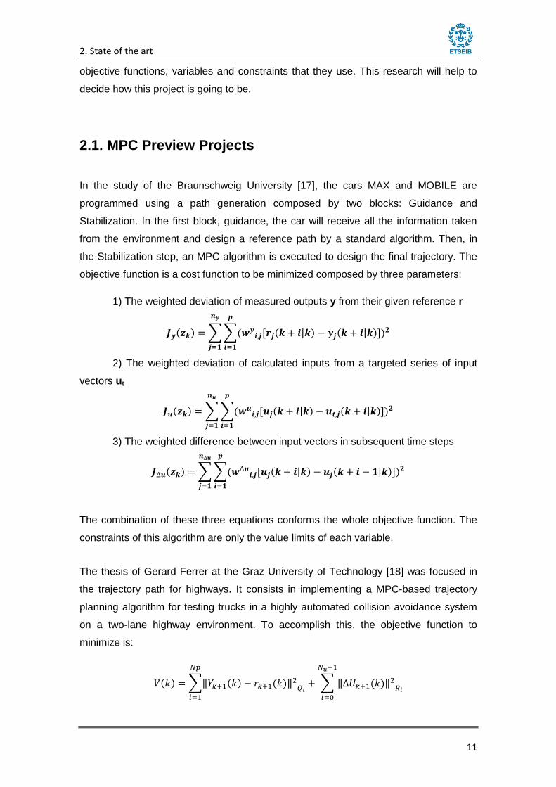
In the study of the Braunschweig University [17], the cars MAX and MOBILE are
programmed using a path generation composed by two blocks: Guidance and
Stabilization. In the first block, guidance, the car will receive all the information taken
from the environment and design a reference path by a standard algorithm. Then, in
the Stabilization step, an MPC algorithm is executed to design the final trajectory. The
objective function is a cost function to be minimized composed by three parameters:
1) The weighted deviation of measured outputs y from their given reference r
𝑱𝒚(𝒛𝒌) =∑∑(𝒘𝒚𝒊,𝒋[𝒓𝒋(𝒌 + 𝒊|𝒌) − 𝒚𝒋(𝒌 + 𝒊|𝒌)])𝟐
𝒑
𝒊=𝟏
𝒏𝒚
𝒋=𝟏
2) The weighted deviation of calculated inputs from a targeted series of input
vectors ut
𝑱𝒖(𝒛𝒌) =∑∑(𝒘𝒖𝒊,𝒋[𝒖𝒋(𝒌 + 𝒊|𝒌) − 𝒖𝒕,𝒋(𝒌 + 𝒊|𝒌)])𝟐
𝒑
𝒊=𝟏
𝒏𝒖
𝒋=𝟏
3) The weighted difference between input vectors in subsequent time steps
𝑱∆𝒖(𝒛𝒌) =∑∑(𝒘∆𝒖𝒊,𝒋[𝒖𝒋(𝒌 + 𝒊|𝒌) − 𝒖𝒋(𝒌 + 𝒊 − 𝟏|𝒌)])𝟐
𝒑
𝒊=𝟏
𝒏∆𝒖
𝒋=𝟏
The combination of these three equations conforms the whole objective function. The
constraints of this algorithm are only the value limits of each variable.
The thesis of Gerard Ferrer at the Graz University of Technology [18] was focused in
the trajectory path for highways. It consists in implementing a MPC-based trajectory
planning algorithm for testing trucks in a highly automated collision avoidance system
on a two-lane highway environment. To accomplish this, the objective function to
minimize is:
𝑉(𝑘) =∑‖𝑌𝑘+1(𝑘) − 𝑟𝑘+1(𝑘)‖2𝑄𝑖
𝑁𝑝
𝑖=1
+ ∑ ‖∆𝑈𝑘+1(𝑘)‖2𝑅𝑖
𝑁𝑢−1
𝑖=0

2. State of the art
12
where Yk+1(k) is the output vector composed by the lateral position and the longitudinal
velocity. This parameter is compared by its reference value to reduce the cost. The
other parameters are taken into a count the variation in subsequent time steps of the
control vector 𝛥U. Moreover, in order to make the collision avoidance, it is implemented
the Nilson’s approach.
In the study of Chang Liu [19], it tries to create a more generic system that can be
implemented in several kind of roads, to be the more versatile as possible. To cover
this complexity of the controller, the objective cost function consists of several different
terms to regulate the behaviour of the vehicle
𝑉(𝑘) = ∑{𝑤𝑔𝑥𝐷𝑘2(𝑥𝑘) + 𝑤𝑔𝑦𝐷𝑘
2(𝑦𝑘) + 𝑤𝑣‖𝑣𝑑 − 𝑣𝑘‖2 +𝑤𝑎‖𝛼𝑘‖
2 +𝑤𝑦𝜔𝑘2
𝑁
𝑘=1
+𝑤𝑗‖𝛼𝑘 − 𝛼𝑘−1‖2 +𝑤ℎ(𝜃𝑁 − 𝜃𝑑)
2}
where Dk2(xk) and Dk
2(yk) are the longitudinal and lateral distance of the current and the
goal position. This will reduce the values while the car is reaching its destination. The
next parameter is a difference between the vehicle’s current speed and the desired
one. Then, the variables ||α||2 and ||ω||2, penalize the large control input, and
minimizing the jerk difference in subsequential time steps.

3. Vehicle modelling
13
3. Vehicle modelling
This chapter will describe the model of the AV which that is going to be used in this
thesis for planning purposes. The AV will consider only the kinematics properties. An
AV is affected by external and internal forces that the motion controller should reject.
This low-level controller will be responsible of optimizing this settings correcting the
possible deviations that the dynamics of the vehicle can generate. Trajectory planners
has an important computational cost, if a dynamic model is included in the trajectory
planner, leading to unfeasible situations of the optimizer in many cases.
Figure 3 Project's block diagram
So, the trajectory planner will generate a valid path considering kinematics properties,
when afterwards the car must track in the considered conditions.
3.1. Kinematic modelling
In order to obtain the kinematic model of the vehicle for the lateral motion, certain
assumptions should be considred [20]. This mathematical model is based on geometric
relationships without considering the forces that affect the motion.
The model considered in this project for the AV is a bicycle model. The model is
considers the two front and rear wheels in one at the centre of each one respectively,
Motion
planner

3. Vehicle modelling
14
as it shown in Figure 4. This two wheels are connected by a wheelbase with a distance
of L and composed by L=lf + lr.
It is assumed that only the front wheel can be steered with an angle of δ, the resulting
angle with the longitudinal axis of the vehicle. The centre of gravity (c.g.) of the vehicle
is in the connection point of lf and lr represented by the point G.
Another assumption is that the vehicle has a planar motion. It is mean that it is only
required to describe the motion the position in axis X and Y to locate the vehicle and
the orientation with the variable θ. Due to these simplications, the velocity vector will be
composed by V as the module and θ the orientation.
Figure 4 Kinematics of lateral vehicle motion
There are two more assumptions that help to define definitely our mathematical model.
It is assumed that the skidding in both wheels is zero. This assumption is only
reasonable for low speed motion of the vehicle. In order to drive on any circular road of
radius, the total lateral force from both tires is:
𝐹𝑙 =𝑚 · 𝑉2
𝑅
If the lateral forces are small due to the small velocity, it can be discounted and
assume that the velocity vector is in the direction of the wheel.
With all this information, the set of kinematic equations of the model the AV are:

4. Formulating of planning
15
{
𝑥𝑘 = 𝑥𝑘−1 + 𝑇𝑠 · �̇�𝑘𝑦𝑘 = 𝑦𝑘−1 · 𝑇𝑠 · �̇�𝑘𝜃𝑘 = 𝜃𝑘−1 · 𝑇𝑠 · �̇�𝑘
{
�̇�𝑘 = 𝑣𝑘 · cos(𝜃𝑘)
�̇�𝑘 = 𝑣𝑘 · sin(𝜃𝑘)
�̇�𝑘 =𝑣𝑘𝑙𝑓· 𝑡𝑎𝑛(𝛿𝑘)
{
�̈�𝑘 =�̇�𝑘 − �̇�𝑘−1
𝑇𝑠
�̈�𝑘 =�̇�𝑘 − �̇�𝑘−1
𝑇𝑠
4. Formulating of planning
4.1. Model Predictive Control
In this chapter, Model Predictive Control (MPC) is reviewed. It is important to
understand how this algorithm works, the objective and the advantages it has. This
information will help the reader to understand why this algorithm is selected and the
functionality of it on the project.
MPC is a control technique that uses a dynamical model to predict its future and then
optimize the control signal. Qin and Badgwell summarize the objectives of an MPC
controller in 2003 [MPC]:
1. Prevent violations of input and output constraints.
2. Drive some output variables to their optimal set points, while maintaining other
outputs within specified ranges.
3. Prevent excessive movement of the input variables.
4. Control as many process variables as possible when a sensor or actuator is not
available.
The MPC calculations are based on current measurements and predictions of the
future values of the outputs. The objective of the MPC control calculations is to
determine a sequence of control moves (that is, manipulated input changes) so that the
predicted response moves to the set point in an optimal manner.

4. Formulating of planning
16
Figure 5 Basic concept for model predictive control.
The advantages that this algorithm presents are:
• It can be used in a wide variety of processes: from simplest to more complex
dynamics.
• It presents inherent compensation to dead-time and time delay phenomena
(even non-minimum phase systems)
• It can be easily extended from the single-variable case to multi-variable case.
• Naturally, it introduces feedforward features in order to compensate
disturbances and measurement noises.
• It can consider constraints over input, state, output and slew-rate variables.
Despite the fact that all these explanations are oriented to control system, MPC has the
advantage that can be very easy adaptable to trajectory generation. It is only needed to
change the definition of the objective function and the constraints to satisfy the
requirements that are necessary.

4. Formulating of planning
17
4.2. Initial data
First, the information that the model and the controller require are described. One of
the most important things in AV is the collection of information of the environment to
manage correctly the driving of the vehicle. In order to optimize and develop a
controller is needed to have enough information to implement all the possible situations
that the AV could face.
This section focus on the initial data that are used by the trajectory planner considering
the corresponding sensors that provides such information. Thus no other important
sensors and variables that are essential for the right driving of an AV will be considered
since they are related to other tasks are the vehicle tracking of the planned trajectory.
Reference Path:
As it was commented the controller generates a path from a reference trajectory
developed previously. This path is composed by the position X and Y, the orientation
and the length of a sample in the entire trajectory. These variables are the reference
that the AV has to follow on the road driving trying to satisfy sequentially these
samples. To generate this reference path it is need a GPS radar. This GPS will identify
the initial and the goal position and using a trajectory planner to generate this reference
path.
Current Car Position:
The software has to know where exactly the car is. This will be used to compute the
difference between the desired and the current position. It is required, as the reference
path, to know the position X and Y, the general orientation (θ) and the length
traversed. To collect this information a GPS can be used providing the X and Y
position, an inertial measurement unit (IMU) for the orientation and an odometer for
measure the distance travelled.
4. Formulating of planning
18
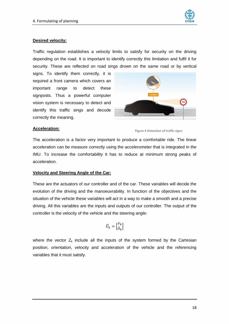
Desired velocity:
Traffic regulation establishes a velocity limits to satisfy for security on the driving
depending on the road. It is important to identify correctly this limitation and fulfil it for
security. These are reflected on road sings drown on the same road or by vertical
signs. To identify them correctly, it is
required a front camera which covers an
important range to detect these
signposts. Thus a powerful computer
vision system is necessary to detect and
identify this traffic sings and decode
correctly the meaning.
Acceleration:
The acceleration is a factor very important to produce a comfortable ride. The linear
acceleration can be measure correctly using the accelerometer that is integrated in the
IMU. To increase the comfortability it has to reduce at minimum strong peaks of
acceleration.
Velocity and Steering Angle of the Car:
These are the actuators of our controller and of the car. These variables will decide the
evolution of the driving and the manoeuvrability. In function of the objectives and the
situation of the vehicle these variables will act in a way to make a smooth and a precise
driving. All this variables are the inputs and outputs of our controller. The output of the
controller is the velocity of the vehicle and the steering angle:
�̂�𝑘 = [𝑣𝑘𝛿𝑘]
where the vector Zk include all the inputs of the system formed by the Cartesian
position, orientation, velocity and acceleration of the vehicle and the referencing
variables that it must satisfy.
Figure 6 Detection of traffic signs

4. Formulating of planning
19
�̂�𝑘 =
[ 𝑥𝑘𝑦𝑘𝜃𝑘�̇�𝑘�̇�𝑘�̇�𝑘�̈�𝑘�̈�𝑘]
�̂�𝑘 = [
𝑥𝑟𝑒𝑓𝑦𝑟𝑒𝑓𝜃𝑟𝑒𝑓𝑣𝑟𝑒𝑓
] �̂�𝑘 = [�̂�𝑘�̂�𝑘]
Despite these data are composed of the inputs and outputs of the MPC controller,
there are other variables that affect directly in the development of the trajectory
generation. One of them is the sampling period that should be configured correctly. A
short period will increase the computational time exponentially and would affect in the
feasibility of the controller while a long period can make the sampling inaccurate giving
an imprecise path.
The other tuning parameter is the prediction horizon. This is determined considering
the number of step-ahead predictions and the sampling time. The first one is the
quantity of estimation in the future the optimizer will do. The second is the interval of
sampling between one prediction and another. These variables depend on the others
factor to be tuned as it will be explained in more detailed in Chapter 6.
4.3. Optimization
In this section, the formulation of the MPC algorithm as an optimization problem will be
described. The objective is to minimize a cost function that will be composed by several
elements that represent the driving performance. Firstly, a collection of terms of
objective function implemented in previous projects is analyzed. Then, all the elements
that conformed the complete algorithm are presented.
4.3.1. Possible objective function elements
After analysing several researches, a compilation of all the factors that were
considered in objective functions considered was done. The goal of this study is to
decide which ones are better to include in the objective function of the proposed
planner.
Position Referencing Cost
This is one of the most important errors to be considered by the palnner. It consists in
the cost related to the difference between the current position of the autonomous

4. Formulating of planning
20
vehicle and the referencing position. It involves position in (x,y) and the orientation (θ).
The objective is to follow the path the most accurate as possible
𝐸𝑝𝑜𝑠 = (𝑥𝑟𝑒𝑓 − 𝑥) · sin(𝜃𝑟𝑒𝑓) + (𝑦𝑟𝑒𝑓 − 𝑦) ∗ cos (𝜃𝑟𝑒𝑓)
𝐶𝑝𝑜𝑠 = 𝐾𝑝𝑜𝑠 · 𝐸𝑝𝑜𝑠2
Velocity Referencing Cost
This cost compares the lineal velocity (v) with the referencing velocity established for
the moment. The linear velocity is one of the output variables of the controller. This
tries to adjust at maximum to the desired velocity fixed. This reference velocity could be
mark by the traffic sings or the situation of the traffic, environment and road
𝐶𝑣𝑒𝑙 = 𝐾𝑣𝑒𝑙 · (𝑣𝑟𝑒𝑓 − 𝑣)2
Acceleration Cost
In order to generate a smooth driving profile, it is interesting to avoid high acceleration
that will be uncomfortable to the passenger. To penalize this behaviour, a cost
penalising the linear acceleration of the vehicle will be considered
𝐶𝑎𝑐𝑐𝑙 = 𝐾𝑎𝑐𝑐 · (𝑎𝑥2 + 𝑎𝑦
2)
Derivative Acceleration Cost
Another cost used to reduce at minimum the acceleration during the driving is to
include the cost involving the derivative of the acceleration. This will penalize strong
peaks of acceleration that are more usual than a constant acceleration
𝐶𝑎𝑐𝑐𝑙 = 𝐾𝑎𝑐𝑐 · (𝑎𝑥𝑇
2
+𝑎𝑦
𝑇
2
)
Steering angle Incremental Cost
Weighted difference between steering angles in subsequent time steps are used to
reduce abrupt turns that generates instabilities in the vehicle and unpleasant driving.
This parameter is especially interesting to collision avoidance manoeuvre and closed
loops

4. Formulating of planning
21
𝐶∆𝜃 = 𝐾𝜃 · (𝛿𝑘 − 𝛿𝑘−1)2
Acceleration Incremental Cost
Another way to control acceleration and avoid hard acceleration is to consider the cost
produced by the acceleration made it by the output velocity. This is a different point of
view changing the control from the state space to the output variables
𝐶𝑎 = 𝐾𝑎 · ((𝑣𝑘 − 𝑣𝑘−1)/𝑇)2
Final Position Cost
This parameter is to encourage the vehicle to achieve the goal position. The objective
of this function is to reduce the cost value during the trajectory execution
𝐸𝑝𝑜𝑠 = (𝑥𝑔𝑜𝑎𝑙 − 𝑥) + (𝑦𝑔𝑜𝑎𝑙 − 𝑦)
𝐶𝑝𝑜𝑠𝑓(𝑘) = 𝐾𝑝𝑜𝑠𝑓 ∗ 𝐸𝑝𝑜𝑠𝑓2
Lateral Error Cost
This parameter calculates the difference between the distance from one limit of the
road or the middle line and the other. The focus of this equation is to achieve the
driving is in the middle of the road respecting the limits to increase the safety
𝐶𝑝𝑜𝑠𝑙 = 𝐾𝑝𝑜𝑠 · (((𝑦𝑙𝑖𝑚𝑖𝑡𝑙 − 𝑦𝑙) − (𝑦𝑙𝑖𝑚𝑖𝑡𝑟 − 𝑦𝑟)) · sin (𝜃𝑟𝑒𝑓))2
4.3.2. Cost function
With the recompilation of all this possible elements, we have to decide which ones will
produce better results. Each one of them improves the behaviour of the vehicle
correcting possible bad manoeuvrability. Although each one leads to benefits to the

4. Formulating of planning
22
trajectory planning, it cannot be selecting of all them since they have conflicting effects.
An excess on the complexity of the cost function will generate some difficulties as the
increase the computation time while losing the importance of some essential terms.
Here, it is presented a table that summarizes the objectives previously presented:
Objective function parameters
Type Cost Equation Importance
Position 𝐶𝑝𝑜𝑠(𝑘) = 𝐾𝑝𝑜𝑠 ∗ 𝐸𝑝𝑜𝑠2 Correct position referred to the path
Velocity 𝐶𝑣𝑒𝑙 = 𝐾𝑣𝑒𝑙 ∗ (𝑣𝑟𝑒𝑓 − 𝑣)2 Correct velocity with the desired one
Linear Acceleration
𝐶𝑎𝑐𝑐 = 𝐾𝑎𝑐𝑐 ∗ (𝑎𝑥2 + 𝑎𝑦
2)
Correct acceleration to 0, trying to avoided acceleration
Dif velocity 𝐶𝑎 = 𝐾𝑎 · ((𝑣𝑘 − 𝑣𝑘−1)/𝑇)2 Correct acceleration
Dif jerk 𝐶∆𝜃 = 𝐾𝜃 · (𝛿𝑘 − 𝛿𝑘−1)2 Correct hard steering
Final Position
𝐶𝑝𝑜𝑠(𝑘) = 𝐾𝑝𝑜𝑠𝑓 ∗ 𝐸𝑝𝑜𝑠𝑓2 Correct the difference between the
actual position and the goal.
Lateral error (((𝑦𝑙𝑚𝑡𝑙 − 𝑦𝑙) − (𝑦𝑙𝑚𝑖𝑟 − 𝑦𝑟)) · sin (𝜃𝑟))2 Correct lateral error
Derivative acceleration 𝐾𝑎𝑐𝑐 · (
𝑎𝑥𝑇
2
+𝑎𝑦
𝑇
2
) Correct hard accelerations
Those one that are marked with green are selected to form the cost function such that
final objective function considered is written as follows:
𝐽𝑘(𝑍𝑘) = ∑𝐶𝑝𝑜𝑠(𝑘) + 𝐶𝑣𝑒𝑙(𝑘) + 𝐶𝑎𝑐𝑐𝑙(𝑘) + 𝐶∆𝜃
𝑁
𝑘=0
(𝑘)
Finally, the cost terms of position, velocity, linear acceleration and incremental of the
steering angle were selected. The reasons for selecting these elements are:
• Position and velocity are essential to be controlled. Using the reference path
the model has to approximate as best as possible the position and orientation.
A recommendable velocity is established such that the vehicle has to keep
constantly along the travelling.
• Linear Acceleration in order to achieve a constant velocity which keeps stable
at the desired velocity. There are two options: the linear acceleration cost and
the velocity difference controlling the output velocity of the controller. It was
decided to select the linear acceleration because on the implementation of the
MPC algorithm, the output prediction has one sample less than the actuators.

4. Formulating of planning
23
• Steering angle in order to increase the comfortability of the manoeuvrability, it
is important that the AV don not turn aggressively. To penalize this behaviour,
the difference of the steering angle for the actual sample and the previous one
is included in the objective function.
These elements have their constant weights (Kpos, Kvel, Kacc, K𝛥δ). These terms has to
be tuned in order to give more or less importance in function of their task. This process
it will be explained in detail in Chapter 6 where it will be explained how the different
costs will affect in a different way in the driving behaviour.
4.3.3 Constrains
This section presents the constraints that will act in the control. Some of them are hard
restrictions from the modelling of the car and others are included for comfort or safety
reasons.
• These variables have some limits to improve the planner computation. The
limits of the position X and Y are the minimum and maximum value of the
coordinates of the reference path, making unable to drive further from this.
• The limits of the orientation is the complete angle of rotation θ ϵ [-π, π].
• The acceleration has a limitation due to the physics of the model, that in this
project it is established by a maximum of amax = ±2 m/s2.
• The velocity restriction that has this model is of vmax = 60 km/h.
• The steering angle interval δ = [-π/6, π/6].
�̂�𝑘:
𝑥𝑚𝑖𝑛 < 𝑥𝑘+1 < 𝑥𝑚𝑎𝑥
𝑦𝑚𝑖𝑛 < 𝑦𝑘+1 < 𝑦𝑚𝑎𝑥
𝜃𝑚𝑖𝑛 < 𝜃𝑘+1 < 𝜃𝑚𝑎𝑥
�̇�𝑚𝑖𝑛 < �̇�𝑘+1 < �̇�𝑚𝑎𝑥
�̇�𝑚𝑖𝑛 < �̇�𝑘+1 < �̇�𝑚𝑎𝑥
�̇�𝑚𝑖𝑛 < �̇�𝑘+1 < �̇�𝑚𝑎𝑥
�̈�𝑚𝑖𝑛 < �̈�𝑘+1 < �̈�𝑚𝑎𝑥

4. Formulating of planning
24
�̂�𝑘:
𝑣𝑚𝑖𝑛 < 𝑣𝑘+1 < 𝑣𝑚𝑎𝑥
𝛿𝑚𝑖𝑛 < 𝛿𝑘+1 < 𝛿𝑚𝑎𝑥
It is important that the controller takes into account the kinematic modelling of
the AV. It is necessary to make feasible outputs that keep the consistency of
the variables during the driving. In order to satisfy these constraints, the
kinematic equations as constraints should be included too. The state space
model in the prediction horizon will enforce that the solution of the actuators
respect the kinematic set of equations and all the state space keep consistent
�̂�𝑘+1 =
[ 𝑥𝑘+1𝑦𝑘+1𝜃𝑘+1�̇�𝑘+1�̇�𝑘+1�̇�𝑘+1�̈�𝑘+1�̈�𝑘+1]
==
[ 𝑥𝑘 + 𝑇𝑠 · �̇�𝑘+1𝑦𝑘 + 𝑇𝑠 · �̇�𝑘+1𝜃𝑘 + 𝑇𝑠 · �̇�𝑘+1𝑣𝑘 · cos(𝜃𝑘+1)
𝑣 · sin(𝜃𝑘+1)�̇�𝑘+1 − �̇�𝑘
𝑇�̇�𝑘+1 − �̇�𝑘
𝑇 ]

5. Solution proposed
25
5. Solution proposed
In this section, the structure of the proposed planner will be presented as well as how it
is implemented using an MPC approach. The proposed solution is programmed and
simulated in MATLAB R2016b.
In order to explain correctly the operation of the planner, it has been divided in four
different parts that it will be explained in detail. These are: Definition of the
environment, MPC controller modelling, Simulation execution and Plotting Results
5.1. Program Structure This is an order list of the execution of the processes in the main program. Apart of the
main program, the project has auxiliary functions that are in charge of other operations.
These are roadComputation, Trajectory_Planner_Reference, Vehicle Evaluation.
These functions are going to be explained in their respectively subchapters. The
execution order of the project is:
1. Establish Variable Limits
2. Compute roadComputation
3. Compute Trajectory_Planner_Reference
4. Determine Desired Velocity
5. Configure MPC controller
6. Simulation loop
6.1 Compute reference point
6.2 Compute SI with the step horizon
6.3 Emergency stops
6.4 Execute the Controller
6.5 Compute Vehicle Evaluation
6.6 Plot the position, steering and velocity
Definition of the environment
MPC controller modelling
Simulation execution
Plotting Results

5. Solution proposed
26
7. Plot lateral error and computational time
5.2. Definition of the Environment
At the beginning of the program, it has to build the entire program environment where
the AV trajectory planner it is going to be simulated. Here, it will set up all the variables,
limits and information that the program needs to create the trajectory correctly.
Firstly, it has to Establish Variable Limits. They are defined variables such as period,
step horizon, the size of the car and the simulation time. It is defined a structure
SimParam which stores all the limits of the inputs and outputs that has been defined on
the Chapter 4.
Secondly, it is called to the function roadComputation. This function is in charge to
define the whole track. It extracts the information of the road circuit from a database
created previously with another program. This database stores Xref, Yref, θref and the
trajectory length. This information is read, adapted and classified. With these data, the
limits on the road are created adding 2 metres on both sides. Thus, the track is one
road in one direction and the optimal driving has to be all the time close to the centre of
the road.
Then, it is implemented the Trajectory_Planner_Reference program. This is in charge
of generating the reference path that the trajectory planner has to create. This program
has another function, detect a possible obstacle on the road and avoid it on the
reference path. The presence of obstacles is identified previously by a computer vision
or LIDAR system. Then, the reference path will follow the road avoiding this obstacle.
Finally, the function ends with the reference path going back to the middle of the road
considering the size of the vehicle and avoiding these obstacles.
Finally, Determine Desired Velocity corresponds to a controlled environment where it is
established a fix desired velocity. The next step would be put the planner in operation
inside the simulation loop and adapt the velocity to the traffic signs. This needs a real
environment with a computer vision program which detects the road signs.

5. Solution proposed
27
5.3 MPC-based planner
The design of an MPC-based planner directly on Matlab could be complex. So, it has
been designed using a toolbox called YALMIP. YALMIP is developed initially for linear
matrix inequalities (LMI) using semidefinite programming (SDP) and interfacing with
external solvers [22]. The toolbox allows the development of optimization problems in
in a very general and simple manner.
Firstly, it has been defined all the variables that are going to take part in the planner:
inputs, outputs, referencing variables and weights. Then, it is established the loop from
1 to N (being N the prediction horizon). In this loop, all the objective function elements
are calculated: Position Referencing Cost, Velocity Referencing Cost, Acceleration
Cost and Steering angle Incremental Cost. Secondly, the variable constraints are
established. Afterwards, it is defined some extra information for the controller. The
most important one is selecting the solver which will solve the optimization problem.
The optimization problem is non-linear so for that reason it was selected the solver
fmincon. Fmincon finds a constrained minimum of a function with four different possible
algorithms: interior point, SQP, active set, and trust region reflective. After defining all
the parameters, inputs, outputs, objective function, solver and options, the MPC
planner can be created.
5.4. Simulation execution
At this point, the program starts creating the path. It is defined by a loop which will be
executing for a determined time or some exceptional errors that make the program
ending.
Firstly, Compute reference point. Here, the desired point where the AV want to arrive is
defined. The difference between the current length and the lengths along the track are
evaluated. The closest point is the one that the model has to achieve.
Secondly, Compute SI with the step horizon. In this process, the desired step horizon
in function with the velocity is determined. To achieve that, the tuning of the SI is
defined by a lineal equation in function of the velocity.

5. Solution proposed
28
Afterwards, the program will check the Emergency stops. Some emergency stops are
created such that will end the program before finishing the time established on the
loop:
The position error is very big: if the trajectory generated goes very far from
the desired reference point it will stop. This will quit the program when the
positional error is intolerable.
The velocity turns to 0. This emergency stop is due to an error that was
frequent in several simulations. This error it is explained in more detail in the
Annex.
The track ends. If the generated planner has reached the last sample of the
reference trajectory, the program will end. This confirms that the planner has
been completed.
Then, the planner will be executed. Before executing the MPC-based planner, it will
collect all the inputs of the current situation of the AV. Afterwards, the planner is
executed with all this information and it will return the optimal output. In case that no
optimal solution is found, it would be assigned a previous output to continue the
simulation.
Finally, Compute Vehicle Evaluation. It will be executed this function to update the
current situation of the AV. Here, the kinematic equation of the model will be simulated
to reproduce the vehicle behaviour. Using the optimal output generated by the MPC
controller, the state space of the AV it will be updated with the current situation.
5.5 Plotting Results
Lastly, the program ends plotting the results of the path. The results are plotted in three
different figures:
1. Current and Reference Position: In this plot, ithe track image with the
representation of the planner will be shown. It will be updated iteratively, adding
the reference point on green and the real position on red. Along the simulation it
will be completed the full track. This image is very representative of how the
MPC planner is developing the trajectory.
2. Velocity and Steering angle: Two grids will be created where the values of the
velocity and the steering angle at each iteration will be added. These two
graphs will help on the analysis. The velocity graph is used to check that the AV

5. Solution proposed
29
is respecting the desired velocity and the steering angle graph to analyse if the
driving is smooth.
3. Lateral error and Computational time: These two graphs are made at the end
of the circuit. In the the first graph, the lateral error of along the whole simulation
is plot to analyse the accuracy of the path. In the second graph, the
computational time required by the MPC planner is shown. This information is
not the most important because they hardly ever are different from different
cases.

6. Tuning
30
6. Tuning
This chapter describes how the parameters of the planner are tuned. The different
issues to be considered to improve and reduce the tuning process will be described.
This information can be helpful if someone wants to introduce this method in their
project. This chapter is divided in the different parameters to be tuned: Position,
velocity, acceleration and sampling instance. The process to be carried out to
achieve to this information can be checked on the Annex: Tuning Process and
Simulation Results.
6.1 Position
This weight is related to the element of position error of the cost function (Kpos) given by
𝐸𝑝𝑜𝑠 = (𝑥𝑟𝑒𝑓 − 𝑥) · sin(𝜃𝑟𝑒𝑓) + (𝑦𝑟𝑒𝑓 − 𝑦) ∗ cos (𝜃𝑟𝑒𝑓)
𝐶𝑝𝑜𝑠 = 𝐾𝑝𝑜𝑠 · 𝐸𝑝𝑜𝑠2
This is one of the most important parameters of the cost function. It determines how
important is to the path generator to follow the reference path generated previously. So
the weight of this parameter has to be significant to have more priority than the other
elements that are not as important.
It is important to the position cost to give it a significant weight to avoid the error but a
non-appropriate value can generate problems as well as insignificant value. This
weight has to take into account these conditions:
If the position parameter is too high, the cost function will give too much
importance to fix the position error that the others objectives are not relevant.
If the position parameter is too high, this could make the trajectory aggressive.
It will not respect the smoothness of the driving and it will try to correct this
position error with hard movements every sample.
If the position parameter is too low, this could make the AV not following the
reference positions and disregard going on the centre of the road.

6. Tuning
31
To explain these concepts, the interval of an optimal functionality of this parameter is
between 100 and 1000. Thus, these values make that the behaviour of the trajectory
will be correct, without taking aggressive movement or without correcting the error.
6.2 Velocity
This weight is related to the element of velocity error of the cost function (Kvel) given by
𝐶𝑣𝑒𝑙 = 𝐾𝑣𝑒𝑙 · (𝑣𝑟𝑒𝑓 − 𝑣)2
The velocity parameter is designed to keep the AV at a constant velocity determined by
the traffic signs. This velocity could change along the route of the vehicle so has to
adapt correctly and keep in that velocity with a reasonable accuracy.
This parameter will keep the vehicle on movement. Thus, it is necessary an important
weight which makes any the deviation of the velocity reference a significant cost. This
weight has to be:
Strong to keep the vehicle on that velocity such that will be the optimal for the
following the track.
Strong to avoid higher velocities that can make the AV overtakes the velocity
limits of the road.
Appropriate to prevent the correct development of the others cost parameters.
As a result of the practice, it was achieved that the correct value of Kvel is between 1
and 50. A number inside this interval will guarantee the correct execution of the velocity
parameter.
6.3 Acceleration
This weight is related to the element of acceleration cost of the objective function (Kacc)
given by
𝐶𝑎𝑐𝑐𝑙 = 𝐾𝑎𝑐𝑐 · (𝑎𝑥2 + 𝑎𝑦
2)
The acceleration is added to eliminate at minimum the accelerations during the driving.
In order to achieve a smooth and comfortable driving, it was established to keep a

6. Tuning
32
constant velocity. Aggressive acceleration is one of the elements that can bother the
passenger during their travel.
In order to make the acceleration weight satisfies its objective and do not disturb the
AV driving its value has to be:
Strong enough to eliminate hard acceleration that can generate bad execution
of the driving.
Strong enough to eliminate aggressive acceleration or deceleration that can
annoy the passenger.
Not too strong to avoid the vehicle start the car and achieve the velocity
reference.
The acceleration constant is the least important parameter of the objective function.
Because of its function is shared with the velocity term, making the acceleration only a
complementary term to reinforce the objective of constant velocity. So, the correct
values of Kacc have to satisfy the conditions established are between 0.1 and 10.
6.4 Steering angle
This weight is related to the element of incremental steering angle of the cost function
(Kθ) given by
𝐶∆𝜃 = 𝐾𝜃 · (𝛿𝑘 − 𝛿𝑘−1)2
The main objective of this parameter is to improve the smoothness and the
comfortability of the driving. It pretends to eliminate hard turns of the AV that would
generate strong centripetal forces that it would bother the passengers.
To achieve this objective the Kθ has to be:
Strong enough to prevent aggressive turns that can destabilize the vehicle and
get worse the comfortability of the driving.
Appropriate to avoid cases where the correct execution of the path can be
affected; making bad sharp curves.
To satisfy these conditions the value of Kθ should be between 0.5 and 20.
6. Tuning
33
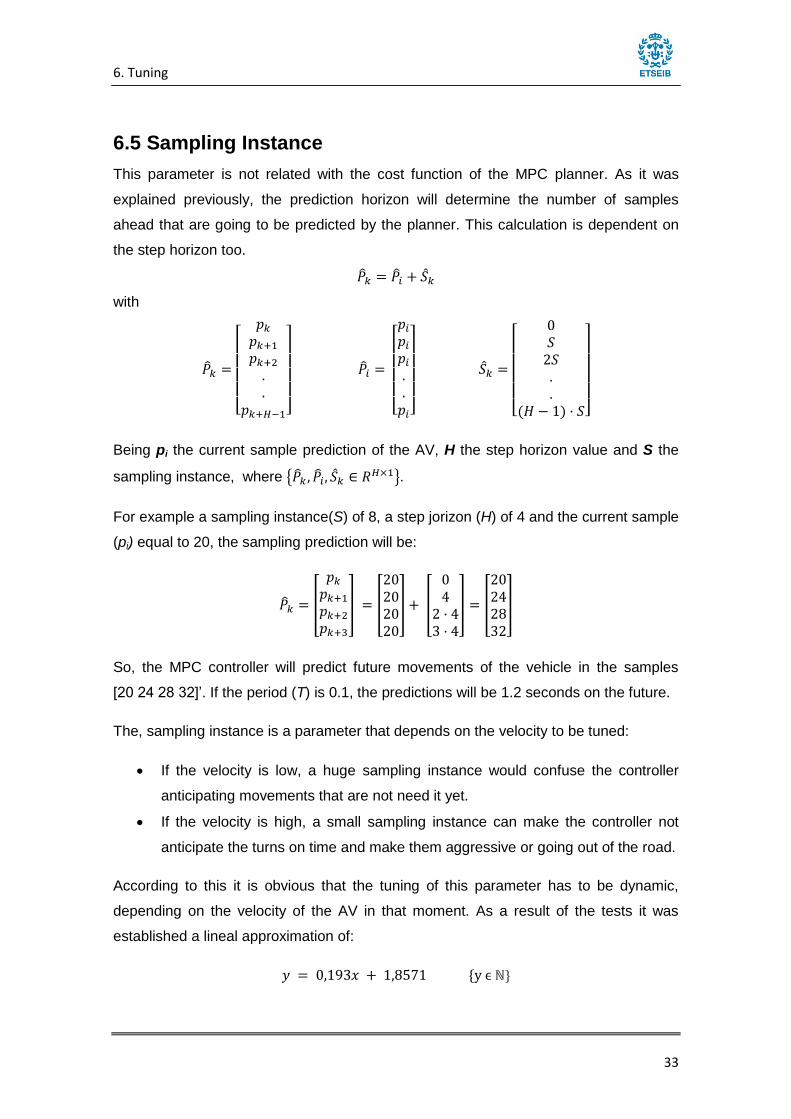
6.5 Sampling Instance
This parameter is not related with the cost function of the MPC planner. As it was
explained previously, the prediction horizon will determine the number of samples
ahead that are going to be predicted by the planner. This calculation is dependent on
the step horizon too.
�̂�𝑘 = �̂�𝑖 + �̂�𝑘
with
�̂�𝑘 =
[
𝑝𝑘𝑝𝑘+1𝑝𝑘+2..
𝑝𝑘+𝐻−1]
�̂�𝑖 =
[ 𝑝𝑖𝑝𝑖𝑝𝑖..𝑝𝑖]
�̂�𝑘 =
[
0𝑆2𝑆..
(𝐻 − 1) · 𝑆]
Being pi the current sample prediction of the AV, H the step horizon value and S the
sampling instance, where {�̂�𝑘 , �̂�𝑖, �̂�𝑘 ∈ 𝑅𝐻×1}.
For example a sampling instance(S) of 8, a step jorizon (H) of 4 and the current sample
(pi) equal to 20, the sampling prediction will be:
�̂�𝑘 = [
𝑝𝑘𝑝𝑘+1𝑝𝑘+2𝑝𝑘+3
] = [
20202020
] + [
042 · 43 · 4
] = [
20242832
]
So, the MPC controller will predict future movements of the vehicle in the samples
[20 24 28 32]’. If the period (T) is 0.1, the predictions will be 1.2 seconds on the future.
The, sampling instance is a parameter that depends on the velocity to be tuned:
If the velocity is low, a huge sampling instance would confuse the controller
anticipating movements that are not need it yet.
If the velocity is high, a small sampling instance can make the controller not
anticipate the turns on time and make them aggressive or going out of the road.
According to this it is obvious that the tuning of this parameter has to be dynamic,
depending on the velocity of the AV in that moment. As a result of the tests it was
established a lineal approximation of:
𝑦 = 0,193𝑥 + 1,8571 {y ϵ ℕ}

7. Results
34
7. Results
This chapter presents the final results of the MPC trajectory planner. To consult all the
simulations obtained ruing the project and look how the tuning process is done in more
detail look the Annex: Tuning Process and Simulation Results. In this chapter, the most
relevant results will be presented which will be used as guidance for define the
configuration of the planner parameters.
There are two tracks that are used to check the efficiency of the trajectory planner. The
first one much simpler consists in one sharp curve and the other on a full circuit.
The first one is used to tune the terms of the objective function: Position, Velocity,
Acceleration and Steering angle. After several tries it converges to these values.
Kvel = 30; Kpos = 500; Kθ = 1; Ka = 1;
With these weights, the best results on lateral error, constant velocity and smoothness
are obtained.
Figure 7 Track 1 and Track 2

7. Results
35
The driving is very accurate with a minimum lateral error, the velocity stays constant all
the time and the turns are very soft.
After tuning the objective terms, the sampling instance was determined. Firstly, it was
tested on the first track with different velocities to adjust the planner parameters
correctly. Here, a table is presented with the results comparing the lateral error
obtained in function of their velocity and sampling instance:
Velocity = 10
V/SI 1 2 3 4 5 6
V= 10 0.0252 0.0239 0.0206 0.0182 1.0087 1.0087
Velocity = 15
V/SI 1 2 3 4 5 6 7 8
15 0.0618 0.0576 0.0532 0.0496 0.0462 0.0426 0.0407 0.9849
Velocity = 20
V/SI 1 4 6 8 9 10 12 18 22 30 36
20 0.395 0.984 0.348 0.335 0.330 0.325 0.315 0.296 0.295 0.318 0.363
Figure 8 Track1: Simulation Results

7. Results
36
Velocity = 30
V/SI 1 2 3 5 6 7 9 30 40
30 8.2375 8.2633 8.2421 8.2490 6.0435 6.7752 6.7347 9.1813 6.0076
Velocity = 40
Unfeasible
The results obtained are only good enough for velocities between 0-20 km/h. The
trajectory generated on velocity 30 and 40 are unfeasible; these velocities are too high
to be dealt by the MPC planner using the kinematic model only.
The next step is to move it to a more complex track. This one will confirm which values
of the Sampling Instance are the bests. The objective is to find these values that can
work correctly in the most number of roads as possible.
The process is to use the sampling instance values which results are the best for each
velocity case. If the value is not good enough, it will be tested the next. The execution
of the trajectory planner on this track supposes a big space of time for each simulation.
So, it could not test as much as it was desired.
The best results that it were obtained are presented in the following.
Velocity = 10
Sampling Instance: 3

7. Results
37
Velocity = 15
Sampling Instance: 5
These two results satisfy the requirements determined and finish correctly the complete
track. Each one presents its advantages and disadvantages:
First result: the lateral error is bigger than the other; it overtakes the 2.5
metres of error. The velocity is very stable but the steering graph
represent some aggressive turns.
Second result: The lateral error is smaller, it does not achieve to the
2.5 metres. On the other hand, the velocity is quite unstable; there are
lots of picks with strong acceleration and deceleration that make worse
the smoothness. The steering angle graph is quite better than the other
one.
If it is needed to decide which presented result is better, it will be chosen the first one.
Although the lateral error is bigger and it is the most important factor to evaluate, the
difference is not too big and the smoothness that this trajectory presents is much better
than the second one.

7. Results
38
But, it should be noted that the main objective of this project is not to find the best one
between all the possibilities, but looking for a general configuration which could be
applied to any situation. The velocity is a dynamic parameter which will be changing in
different situations. So, as it was commented on the previous chapter, the important of
this simulation is to find a configuration adapted for different conditions.
To make this dynamic tuning is collected the best results of the simulations on the track
2, being:
S v
10 3
15 5
20 7
30 7
This approximation is very simple and not very representative. It should be done more
trials in different tracks to adjust better this equation.

8. Effects on economy, society and environment
39
8. Effects on economy, society and
environment
The technology is one of the most powerful tools to change radically the world and a
strong technological advance means a modification of the economy, society and
environment. In this chapter, the possible impact that this project can have is going to
be discussed. Being this project a research on AV, this section will be oriented more in
how AV can impact in the economy and society.
8.1. Economic impact
Car industry is one of the most powerful of the whole market. It is a sector which needs
a powerful manufactory which requires thousands of millions to generate its product.
This sector is very linked with technological developments and it is necessary to be
leading on its field. Technological improvement on their product supposes more
attractive products that suppose an increment of sales.
In 2017, car industry sales are more than 90 millions of units [23]. These data is in a
market that is more or less stable during these years, where AVs are not already on the
market and electrical vehicles have not excelled yet. Nowadays people still buying
manual and petrol cars, but this seems to change. The evolution of the car industry in
the next years will be drastic. People will start to change their old fuel cars for electric
and autonomous. This replacement for manual to AV will generate an increment on
sales to adapt their vehicles to the new driving system.
On top of that, autonomous driving can be applied to other ways of transport. It is only
necessary to adapt the theory to each different sector being very interesting for
activities as e.g. delivery drones.
Advances on important parts like trajectory generation could help to companies that
work with the university to implement these techniques and improve their AV systems.
Companies that have headquarters in Catalonia like Seat or Nissan can take
advantages of this research.

8. Effects on economy, society and environment
40
8.2. Social and environmental impact
Autonomous driving has a big impact on the society. It will change totally the concept of
travelling from one point to another.
Firstly, it will increase the safety on the roads. Only in Spain in 2016, there was an
important number of fatal accidents that suppose 1.160 deaths and 5.067 casualties
needing hospital treatment in general [24]. The majority of these accidents are by
human error. So, these numbers would be reduced when AV substitute the actual
ones.
The comfortability during the travelling it will be increased. Due to the optimal driving
that AV will generate and the reduction of traffic accidents, jams will almost disappear.
A smoother driving without aggressive manoeuvrability or strong acceleration will
reduce the travel sickness. Furthermore, the mobility of people with disabilities AND old
people will be enhanced.
The execution of an optimal driving will generate a reduction of the pollution too. If it is
a fuel car, it will reduce the consumption of fuel and if it is an electrical one it will reduce
the use of electrical power. In both cases, a reduction of energy will imply improving the
efficacy and making less environmental impact. Furthermore, the number of vehicles
on the street can be reduced by an idea of a net of connected cars available to share
between several people.
9. Project budget
41
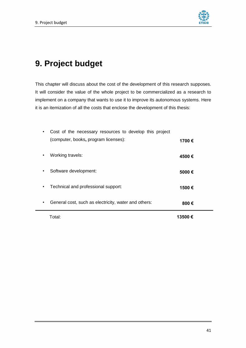
9. Project budget
This chapter will discuss about the cost of the development of this research supposes.
It will consider the value of the whole project to be commercialized as a research to
implement on a company that wants to use it to improve its autonomous systems. Here
it is an itemization of all the costs that enclose the development of this thesis:
• Cost of the necessary resources to develop this project
(computer, books, program licenses):
• Working travels:
• Software development:
• Technical and professional support:
• General cost, such as electricity, water and others:
1700 €
4500 €
5000 €
1500 €
800 €
Total: 13500 €

10. Conclusions and Future Work
42
10. Conclusions and Future Work
10.1 Conclusions
This project deals with one of the most important parts of AV: trajectory generation.
The solution implemented is based on MPC-based planner that converts a trajectory
problem in an optimization problem. The implementation involves several processes.
Firstly, the multiple trajectory algorithms already implemented for autonomous cars
have been reviewed. After analyzing their advantages and disadvantages, it has been
decided to implement a MPC-based planner. Its main advantages are the possibilities
to make an online trajectory generation and to develop a realistic trajectory path
subject to kinematic constrains. To select the elements of the objective functions,
several studies were consulted. IAll the parameters used on these studies were
collected and at the end the most interesting ones were selected.
Secondly, the MPC-based planner was created and the corresponding parameters
(weights) tuned. The tuning was done on a first track. Firstly, the elements of the
objective function were tuned. Then, the sampling instance in function of the velocity
was characterized.
Finally, it was tested on the second track. Here, it was decided which sampling
instances are the best regarding the velocity. Then, a dynamic tuning of the planner
parameters is developed using a linear function of the velocity. During all this process it
was concluded that:
MPC planner has many interesting advantages compared with the other
planner algorithms. The most important are:
o Online execution that can modify its path in case of unexpected
changes on the road.
o Simplicity, translating the planning problem into an optimization
problem.
o Realistic, making the trajectory be subjected to the kinematic equations
of the model.
o Versatility, in the creation of the controller.

10. Conclusions and Future Work
43
o Prevent violations of input and output constraints.
MPC planner has many interesting advantages compared with the other
planner algorithms. The most important are:
o The importance of a good tuning to be the most general as possible. It
cannot be completely independent; it must be related with the situation
of the car and the environment.
o The obtained results are satisfactory and the use of this algorithm as a
trajectory generation of an AV is completely feasible.
o The potential that this algorithm presents is enormous. This only work
with the bases of the algorithm but it can be improved a lot adding new
external systems.
10.2 Future works
As it was said in the last point of the conclusions, the proposed algorithm can be
improved in many ways. Thanks to the orientation of an optimization problem, external
functions and information can be added and applied in a very easy way.
One example is to introduce a computer vision system to detect the velocity. During the
simulation where the planner is being created, a computer vision system can be added
to detect the velocity limits and adjust the velocity reference at every sample. This will
make the driving adaptable to every situation of the road satisfying the velocity
requirements of the road.
Another possible improvement is to tune the sampling instance in relation of the
curvature of the road. It was detected that depending on the type of the curve it is
better one value or other. So, a dynamic tuning of this parameter in relation not only
with the velocity, but with the curvature of the road can make a stable algorithm that
can face any type of tracks.
Finally, the most obvious and important continuation of this project is the
implementation of the program in a real system. All this research it has been done in a
theoretical way with computer simulations. The most important is to observe how the
algorithm works on a real system with its difficulties that this sets out.
ANNEX Tuning Process and Simulation Results
44
ANNEX Tuning Process and Simulation
Results
Introduction
After selecting all the parameters that composed the objective function, it has to be set
the correct weights. This is a tough process which it is need to configure logical
hypothesis with a process of trial and error. It is has to be configured the weights of the
“lateral error”, “velocity error”, “increment of steering angle”, the “acceleration cost” and
“sampling instance”. To tune these variables it is going to be analysed the behaviour of
the AV in several environment with different characteristics. The objective is to fine a
constant set of weights that can develop a good trajectory in different situations or
create dynamic values that are going to be adapted to the configuration of the road.
Furthermore, it has to decide which information is going to be examined to decide
which tuning set is better than the other. This can be different between different
projects and it depends on how the model and the optimizer work. For our case, the
position error from the reference one is the most important information. It is obvious
that a huge position error that can make the car go outside from the road is not
tolerated. The second most important data that is analysed is the steering graph. The
behaviour of the maneuverer of the AV is reflected on how this parameter carries out.
So it is going to priories smooth slopes at the curves avoiding tough turns that can
make the driving uncomfortable to the passenger. Finally, the last variable that is going
to be considered is the velocity of the car. It is important that the car achieve the
desired velocity and stay constant along the way and adapt the changes correctly.
First Track
The first track where the car behaviour is going to be analysed is the simplest one. It
consists of a straight road with a tough curve of 180º and another road in the opposite
direction.

ANNEX Tuning Process and Simulation Results
45
Second Track
The second track is more complex. It combines several curves and shapes that
increase the difficulty and its length. Here it is where the program would present more
difficulties and help us to decide the correct tuning.
Tuning Objective Function
Thanks to a previous project, it can be taken some information as help to this project.
Eugeni’s project has an objective function quite similar as this project, controlling the
lateral error, the velocity difference and the existence of acceleration. It is executed this
controller in the first track to see the results.
The weights programmed are Kpos=1, Kvel=500, and Kacc=0.1.

ANNEX Tuning Process and Simulation Results
46
As it can see the model has quite good results to establish these weights as a starting
point of the tuning. The objective function of that it would want to design has
differences. It includes a steering angle control parameter to avoid aggressive
manoeuvres.
𝐽𝑘(𝑍𝑘) = ∑𝐶𝑝𝑜𝑠(𝑘) + 𝐶𝑣𝑒𝑙(𝑘) + 𝐶𝑎𝑐𝑐𝑙(𝑘) + 𝐶∆𝜃
𝑁
𝑘=0
(𝑘)
It was studied the possibility to include an acceleration control parameter that actuate
directly on the output controller eliminating the Cartesian one. But how both
acceleration controllers are quite similar the results were the same. So it was
concluded to use the Cartesian acceleration controller to simplicity on the development
of the MPC.
The next step is to include the steering angle parameter and try to tune all the system
again. After several trials, it has observed that the magnitude worked between this
parameter and the others are very important, so the tuning is very difficult to do. The
solution is to normalize all the parameter of the objective function, to work with all the
magnitude on unitary values.
This modification makes that the weighted tuning changes drastically and starts from
the beginning. To help this process, it was configure the program to plot all the error
cost, normalized and no normalized, to see which their behaviour are and how different
they are. The idea is to approximate, tuning the weights, to the initial objective function
costs. After analysing this data, it was observed that the behaviour is quite similar and

ANNEX Tuning Process and Simulation Results
47
with a magnitude 10 times less than the non-normalized parameters. So these are
several results that it was obtained:
Simulation 1.1: Kvel = 10; Kpos = 100; Kθ = 0; Ka = 1;
Simulation 1.2: Kvel = 10; Kpos = 500; Kθ = 0; Ka = 1;
Simulation 1.3: Kvel = 40; Kpos = 1000; Kθ = 0.5; Ka = 1;

ANNEX Tuning Process and Simulation Results
48
Simulation 1.4: Kvel = 20; Kpos = 1000; Kθ = 10; Ka = 10;
From all these results it can select 2 tuning weights that work correctly. The first one is
the Simulation 1.1 and the Simulation 1.4. Each one has its advantages. The
simulation 1.1 has a higher position error arriving to a 1 m of distance but with a
smoother manoeuvre as it can see in the steering graph. From the other side, the

ANNEX Tuning Process and Simulation Results
49
Simulation 1.4 has a very low position error with a maximum of 0.12 but a worse driving
with many turns and not a constant direction. So for the next road circuit it is going to
check how this parameter works.
Tuning Sampling Instance (Normalized Parameters)
The next step after getting the weights of the objective function is to tune the sampling
instance of the program. The sampling instance will determinate how many samples
will go ahead to make their predictions. This parameter is much related with the
velocity:
A low velocity with a big sampling instance can confuse the controller making
their curves before and or in a different way
A high velocity with a small sampling instance would make the car not predict
their curves fast enough to go all over the road.
These are our logical hypothesis, but it is needed to determinate which sampling
instance can be defined as small or big. There are other parameters that influence this
process one of them is the sample period. On this program is establish as T=0.1s. The
second is the step horizon. This will determine how many sampling instances intervals
will be predicted. This parameter for computational cost it was established as 4. A big
number on the step horizon can improve the driving of the AV but would mean an
increment of the computational time that it can be afforded. So to calibrate this
parameter it was done many simulations to determine the optimal step for each
velocity:
The objective function weights are: Kvel = 20; Kpos = 1000; Kθ = 10; Ka = 10;
Velocity: 10 Sampling Instance: 1
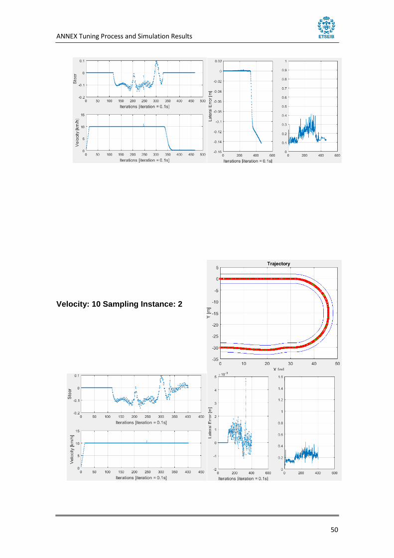
ANNEX Tuning Process and Simulation Results
50
Velocity: 10 Sampling Instance: 2

ANNEX Tuning Process and Simulation Results
51
Velocity: 10 Sampling Instance: 5
Velocity: 10 Sampling Instance: 6

ANNEX Tuning Process and Simulation Results
52
Velocity: 10 Sampling Instance: 1
Velocity: 10 Sampling Instance: 2

ANNEX Tuning Process and Simulation Results
53
Velocity: 10 Sampling Instance: 3
Velocity: 10 Sampling Instance: 4

ANNEX Tuning Process and Simulation Results
54
Velocity: 10 Sampling Instance: 5
Velocity: 10 Sampling Instance: 6

ANNEX Tuning Process and Simulation Results
55
The results are not as satisfactory as it was expected. Specially for a strange behaviour
in several results. Such as in simulations:
Track 1 V=10 SI=1
Track 1 V=10 SI=5
Track 2 V=10 SI=3
At the middle of the execution, the velocity starts to decrease its velocity even though
the AV is doing correctly the track. As it can see on the results this event has not
relationship with the sampling instance, it appears randomly.
The first though was related with the desired position that has to achieve. Probably it
tries to achieve desired points that are backward on its own position for that reason
start to decelerate. Apparently the program works correctly; it always searches a step
ahead point to achieve. It was integrated some exclusive solutions for this situation.
Firstly an increase on the desired point, in order to increment the position error; this
can encourage the system. Secondly a change on the step horizon, trying on those one
that this problem didn’t happen. All these solutions were a failure.
The second tough was related with the objective function weights. It was incremented
the velocity and the acceleration weights. This makes more expensive to not keep the
desired velocity and decelerate. After several trials changing these values it was not
possible to fix it, it seems that is not related with this concept.
Finally it was discovered that this issue wasn’t usual when the values were not
normalized. Maybe this operation give a resulting values that can make the MPC
controller get confused in several situation. So it was decided to eliminate this
normalization.
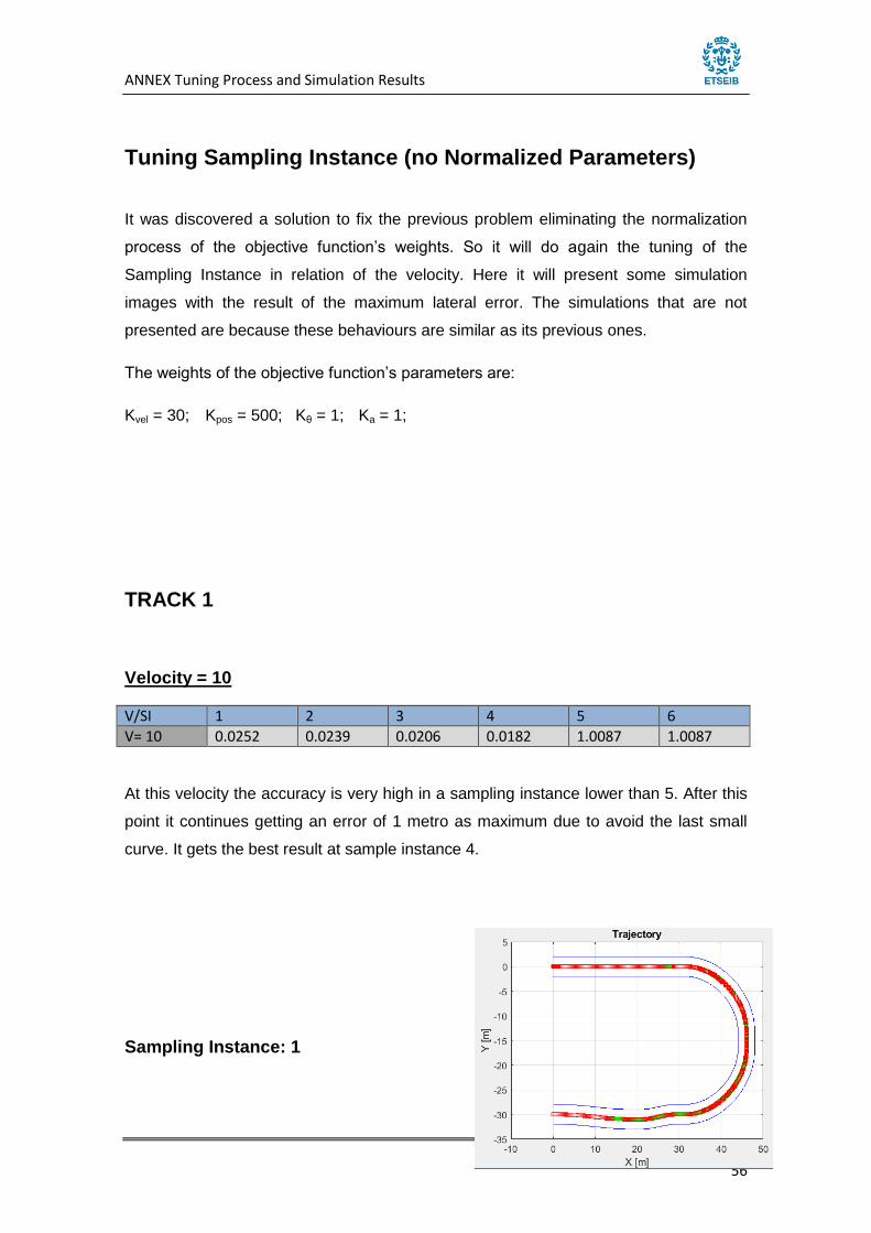
ANNEX Tuning Process and Simulation Results
56
Tuning Sampling Instance (no Normalized Parameters)
It was discovered a solution to fix the previous problem eliminating the normalization
process of the objective function’s weights. So it will do again the tuning of the
Sampling Instance in relation of the velocity. Here it will present some simulation
images with the result of the maximum lateral error. The simulations that are not
presented are because these behaviours are similar as its previous ones.
The weights of the objective function’s parameters are:
Kvel = 30; Kpos = 500; Kθ = 1; Ka = 1;
TRACK 1
Velocity = 10
V/SI 1 2 3 4 5 6
V= 10 0.0252 0.0239 0.0206 0.0182 1.0087 1.0087
At this velocity the accuracy is very high in a sampling instance lower than 5. After this
point it continues getting an error of 1 metro as maximum due to avoid the last small
curve. It gets the best result at sample instance 4.
Sampling Instance: 1

ANNEX Tuning Process and Simulation Results
57
Sampling Instance: 2
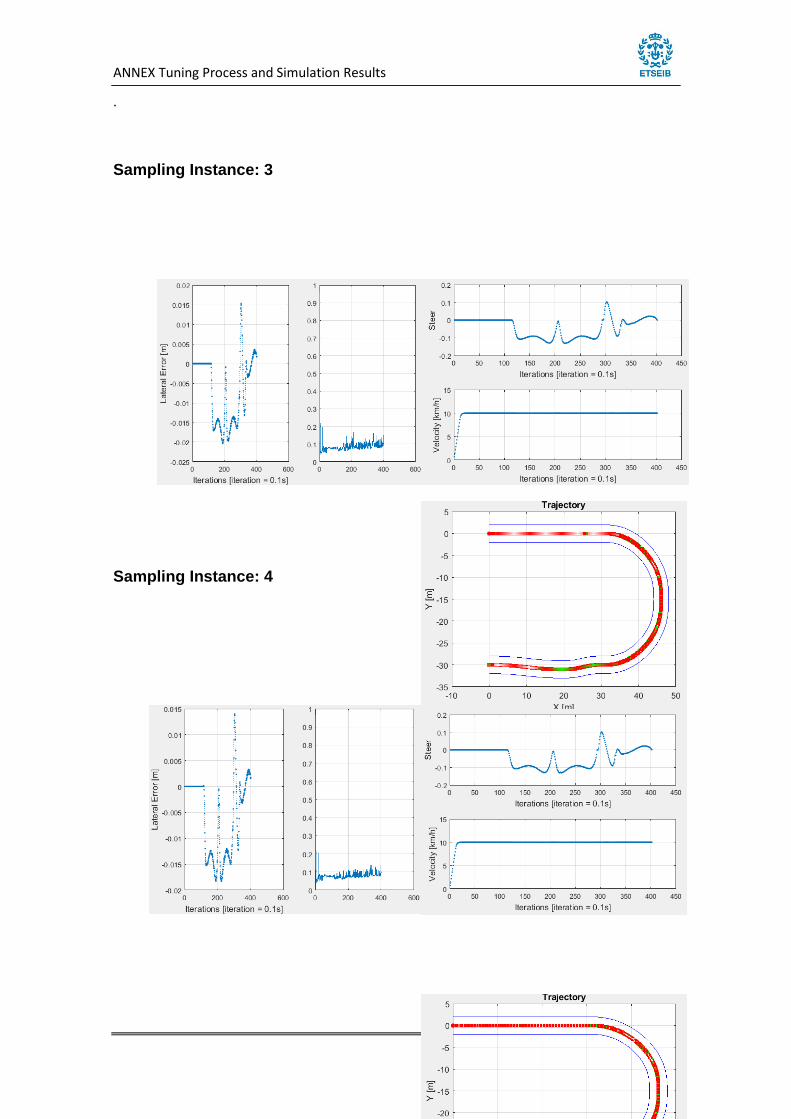
ANNEX Tuning Process and Simulation Results
58
.
Sampling Instance: 3
Sampling Instance: 4

ANNEX Tuning Process and Simulation Results
59
Sampling Instance: 5
Velocity = 15
V/SI 1 2 3 4 5 6 7 8
15 0.0618 0.0576 0.0532 0.0496 0.0462 0.0426 0.0407 0.9849
These simulations have very good results too. They have a good accuracy with a good
manoeuvrability until arriving to the SI 8. Since SI 8, the model starts to avoid the last
small curve getting a bigger lateral error on this moment
Sampling Instance: 1

ANNEX Tuning Process and Simulation Results
60
Sampling Instance: 2

ANNEX Tuning Process and Simulation Results
61
Sampling Instance: 8
Velocity = 20
V/SI 1 4 6 8 9 10 12 18 22 30 36
20 0.395 0.984 0.348 0.335 0.330 0.325 0.315 0.296 0.295 0.318 0.363
Velocity 20 has the most solid results. It has a good execution even though the
accuracy is not as good as the other ones. There is an exception with SI in 4. It was
concluded that MPC is very influenced on the chosen samples. This sample selection
can generate strange execution plans if does not represent correctly the reality of the
path. Surprisingly, the most accurate results are in SI 22. It is a bigger sampling
instance that it was thought.
Sampling Instance: 1

ANNEX Tuning Process and Simulation Results
62
Sampling Instance: 4

ANNEX Tuning Process and Simulation Results
63
Sampling Instance: 6
Sampling Instance: 8

ANNEX Tuning Process and Simulation Results
64
Sampling Instance: 10
Velocity = 30
V/SI 1 2 3 5 6 7 9 30 40
30 8.2375 8.2633 8.2421 8.2490 6.0435 6.7752 6.7347 9.1813 6.0076
With this velocity it hasn’t achieve any convincing results. All of them have a big lateral
error of several meters and didn’t finish on the goal position. The best result of all of
them is with a Sampling Instance of 40, but it cannot consider a good result either.
Sampling Instance: 1

ANNEX Tuning Process and Simulation Results
65
Sampling Instance: 6

ANNEX Tuning Process and Simulation Results
66
Sampling Instance: 30
Sampling Instance: 40

ANNEX Tuning Process and Simulation Results
67
VELOCITY = 40
At this velocity the planner was unable to develop a successful path. The velocity is too
high that make infeasible to execute this sharp curve. It was simulated with several
Sampling Instance but all the results were the almost the same. It gets lost when it
wasn’t able to do this track.
Sampling Instance: 4

ANNEX Tuning Process and Simulation Results
68
TRACK 2
Now it is going to test the MPC controller on a more complex track composed of
several curves. This it will guarantee which Sampling Instances are good for any other
trajectories. The order that is going to follow is:
Firstly, check the Sampling Instance that obtained the best results on the
previous simulations.
If the results are not convincing or it was estimate that with other sampling
instances it can get the same or best results they will be tried.
Due to the computational time of the simulation of the whole track is enormous (mainly
for the use of Matlab plots) in most of the cases are only simulated the first half of the
track. Assuming that the first half of the track is the more complex one, if the program
gets a good result, it will assume that it can finish the whole track with the same
behavior. Some of the results are incomplete because of the saturation of the Ram
made impossible to get the last graphs.
Velocity = 10

ANNEX Tuning Process and Simulation Results
69
Sampling Instance: 4
Sampling Instance: 3

ANNEX Tuning Process and Simulation Results
70
The first Sampling Instance that was tried is with the value 4. As it can see the results
seems good enough. The trajectory follows correctly the road. It will assume that it will
end the track correctly.
It was checked the possibility that with a different Sampling Instance it continues
getting good results. It was checked with S=3. That was the second best result of the
track 1. It will let until the end of the track to check if it can finish correctly. The results
were better than the first one. Finishing the full track and obtaining a lateral error lower.
Velocity 15
Sampling Instance: 7
Sampling Instance: 5

ANNEX Tuning Process and Simulation Results
71
With velocity of 15 the optimal is achieved on the sampling instance of 5 instead of 7.
Velocity = 20
Sampling Instance: 22
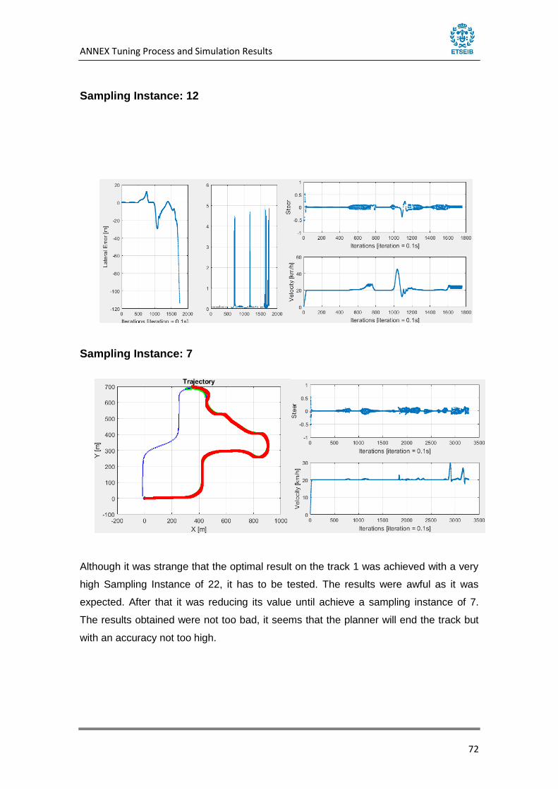
ANNEX Tuning Process and Simulation Results
72
Sampling Instance: 12
Sampling Instance: 7
Although it was strange that the optimal result on the track 1 was achieved with a very
high Sampling Instance of 22, it has to be tested. The results were awful as it was
expected. After that it was reducing its value until achieve a sampling instance of 7.
The results obtained were not too bad, it seems that the planner will end the track but
with an accuracy not too high.

ANNEX Tuning Process and Simulation Results
73
VELOCITY = 30
Sampling Instance: 7

ANNEX Tuning Process and Simulation Results
74
Sampling Instance: 9
As a result of the behaviour of the trials on the case of velocity is 20, it was discarded
the highest values of the Sampling Instance despite that they were the best ones on
the track 1. It was started with 7, because it was the best result obtained on the
previous simulations. The planner couldn’t end the track, so the sampling instance was
increased until 9.

11. Bibliography
75
11. Bibliography
[1] Robot Glob. Evolution of Self Driving Autonomous Car - Retrieved 2018-06-24 [2] Digital Trend. Sit back, relax, and enjoy a ride through the history of self-driving
cars - Retrieved 2018-06-24 [3] Waymo Journey. The Google self-driving car project began - Retrieved 2018-
06-24
[4] BI Intelligence. 10 million self-driving cars will be on the road by 2020 - Retrieved 2018-05-24
[5] Todd Litman. Autonomous Vehicle Implementation Predictions – Victoria
Transport Policy Institute April 2018 [6] Protivity Insights. The Evolution of Autonomous Vehicles –Retrived 2018-06-24 [7] VentureBeat. The Most Important Self-Driving Car Announcement Yet - 2018-
05-08. Retrieved 2018-05-24. [8] MIT News Self-driving cars for country roads May, 2018. Retrieved 2018-05-24

11. Bibliography
76
[9] Gonzalez D., Pérez. J., Milanes V. and Nashashibi. F A Review of Motion Planning Techniques for Automated Vehicles. November 2015
[10] S. M. LaValle, Planning algorithms. Cambridge university press, 2006.
[11] M. Likhachev and D. Ferguson, “Planning long dynamically feasible maneuvers
for autonomous vehicles,” The International Journal of Robotics Research, vol.
28, no. 8, pp. 933–945, 2009.
[12] M. Pivtoraiko and A. Kelly, “Efficient constrained path planning via search in
state lattices,” in International Symposium on Artificial Intelligence, Robotics,
and Automation in Space, 2005.
[13] M. Elbanhawi and M. Simic, “Sampling-based robot motion planning: A review,” Access, IEEE, vol. 2, pp. 56–77, 2014.
[14] M. Elbanhawi and M. Simic, “Sampling-based robot motion planning: A review,”
Access, IEEE, vol. 2, pp. 56–77, 2014.
[15] M. Brezak and I. Petrovic, “Real-time approximation of clothoids with bounded
error for path planning applications,” Robotics, IEEE
[16] D. Dolgov, S. Thrun, M. Montemerlo, and J. Diebel, “Path planning for
autonomous vehicles in unknown semi-structured environments,” The
International Journal of Robotics Research, vol. 29, no. 5, pp. 485–501, 2010.
[17] Marcus N., Marcel R., Torben S. and Markus M. Model Predictive Control Based Trajectory Generation for Autonomous Vehicles – An Architectural Approach
[18] Gerard F. Trajectory generation for Autonomous Highway Driving using Model
Predictive Control - September 2017 [19] Chang L., Seungho L., Scott V., H. Eric T. Path Planning for Autonomous
Vehicles using Model Predictive Control. 2017 IEEE Intelligent Vehicles Symposium (IV)
[20] RAJAMANI, R. Vehicle Dynamics and Control. Springer, 2012. [21] Dale E. Seborg Process Dynamics and Control Wiley (2010) [22] Johan LöfberG YALMIP : A toolbox for modeling and optimization in MATLAB -
October 2004
[23] Bart Demandt. Global car sales analysis 2017 Retrived 2018-06-11 [24] Spain DGT report on 2016 road fatalities- Tumbit Retrieved 2018-06-11

11. Bibliography
77