A visual navigation system for autonomous land vehicles
18
124 IEEE JOURNAL OF ROBOTICS AND AUTOMATION, VOL. RA-3, NO. 2, APRIL 1987 A Visual Navigation System for Autonomous Land Vehicles ALLEN M. WAXMAN, MEMBER, IEEE, JACQUELINE J. LEMOIGNE, LARRY S. DAVIS, MEMBER, IEEE, BABU SRINIVASAN, TODD R. KUSHNER, MEMBER, IEEE, ELI LIANG, AND THARAKESH SIDDALINGAIAH Abstract-A modular system architecture has been developed to support visual navigation by an autonomous land vehicle. The system consists of vision modules performing image processing, three-dimen- sional shape recovery, and geometric reasoning, as well as modules for planning, navigating, and piloting. The system runs in two distinct modes, bootstrap and feedforward. The bootstrap mode requires analysis of entire images to find and model the objects of interest in the scene (e.g., roads). In the feedforward mode (while the vehicle is moving), attention is focused on small parts of the visual field as determined by prior views of the scene, to continue to track and model the objects of interest. General navigational tasks are decomposed into three categories, all of which contribute to planning a vehicle path. They are called long-, intermediate-, and short-range navigation, reflecting the scale to which they apply. The system has been implemented as a set of concurrent communicating modules and used to drive a camera (carried by a robot arm) over a scale model road network on a terrain board. A large subset of the system has been reimplemented on a VICOM image processor and has driven the DARPA Autonomous Laud Vehicle (ALV) at Martin Marietta’s test site in Denver, CO. I. INTRODUCTION T HIS PAPER describes the organization of a system for visual navigation of roads and road networks. The objective is to endow a mobile robot vehicle with the intelligence requiredtosense and perceive that part of its surroundings necessary to support navigational tasks. The vehicle maintains continuous motion by alternatively “looking ahead” and then “driving blind” for a short distance before taking another view. While moving blindly, the accepted monocular image is processed to extract features which are then interpreted in three dimensions by a combination of “shapefromcontour” and geometricreasoning.This pro- vides the data required to form an object-centered representa- tionin the form of a local map. This map is used both for navigation and for focusing attention on selected parts of the visual field as the vehicle continues to move, accepting new images for processing. Though our domain of application has Manuscript received October 29, 1985; revised August 13, 1986. This work was supported in part by the Defense Advanced Research Projects Agency and the US Army Engineering Topographic Laboratories under Contract DACA76-84-C-0004. A. M. Waxrnan was with theComputer Vision Laboratory,Centerfor Automation Research, University of Maryland, College Park, MD, USA. He is now an Assistant Professor in the Department of Electrical, Computer & Systems Engineering, Boston University. 110 Cummington St., Boston, MA 02215, USA. J. J. LeMoigne, L. S. Davis, T. R. Kushner, E. Liang, and T. Siddalingaiah are with the Computer Vision Laboratory, Center for Automa- tion Research, University of Maryland, College Park, MD 20742, USA. B. Srinivasan was with the Computer Vision Laboratory, Center for Automation Research, University of Maryland, College Park, MD, USA. He is now with FMC Corporation, Central Engineering Laboratories, 1185 Coleman Avenue, Box 580, Santa Clara, CA 95052, USA. IEEE Log Number 8613005. been the visual navigation of roadways, we have attempted to derive some useful principles relevant to visual navigation systems in general. Our preliminary efforts on this work have been reported in [I]. A variety of design philosophies for mobile robot systems have been discussed in the literature [2]-[7], and our approach has some features in common with them. The guiding principles that have emerged from our research touch on three areas of design. The first concerns the modularity of the system architecture, in which a distinction is made between computational capabilities within modules, the nature of the representations that enter and leave these modules, and the flow of control through the system. The second deals with the nature of the focus of visual attention in the system. Thisleads to significant computational savings and greater vehicle speeds. The third is a decomposition of general navigation tasks into three categories which support navigation on three different scales. The construction of a modular system architecture is attractive for a variety of reasons. Individual modules can possess well-defined responsibilities and consist of several related computational capabilities. The behavior that the vehicle itself exhibits then reflects the “flow of control” through the modules of the system. This decomposition into modules also points to the importance of the interfaces that link modules, for it is across these interfaces that intermediate representations of the processed data travel as well as the control commands which govern the choice of computations within modules. Modularity also opens the door to distributed parallel processing, with various modules possibly running on dedicated hardware. For example, some of our image process- ing routines, developed on a VAX 11/785, have been adapted to run on a VICOM image processor [8]. We will describe the modules which comprise our system, their current and planned capabilities for .the future, and the flow of control which supports road following. We have found it useful to distinguish between two different modes of visual processing, and our system can switch between these modes when necessary. Generally, the system begins a task in the bootstrap mode which requires process- ing an entire scene, picking out the objects of interest such as roads or landmarks. Sometimes this modeof processing can be avoided ifthe system is provided with detailed data concerning the location of such objects, either from a map or from the analysis of previous sensed data. Once objects of interest are identified, the system switches to a prediction-verification mode called feedforward in which the location of an object as seen from a new vehicle position is estimated, thus focusing 0882-4967/87/0400-0124$01 .OO 0 1987 IEEE
-
Upload
independent -
Category
Documents
-
view
3 -
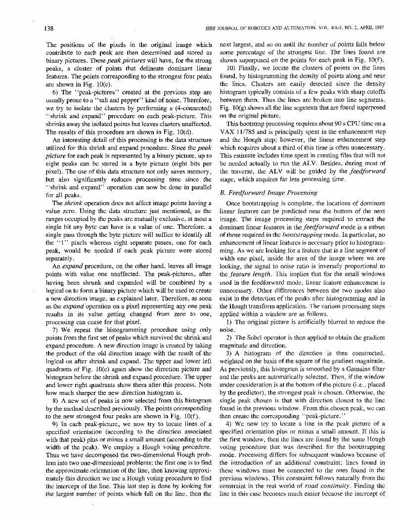
download
0
Transcript of A visual navigation system for autonomous land vehicles
124 IEEE JOURNAL OF ROBOTICS AND AUTOMATION, VOL. RA-3, NO. 2, APRIL 1987
A Visual Navigation System for Autonomous Land Vehicles
ALLEN M. WAXMAN, MEMBER, IEEE, JACQUELINE J. LEMOIGNE, LARRY S. DAVIS, MEMBER, IEEE, BABU SRINIVASAN, TODD R. KUSHNER, MEMBER, IEEE, ELI LIANG, AND
THARAKESH SIDDALINGAIAH
Abstract-A modular system architecture has been developed to support visual navigation by an autonomous land vehicle. The system consists of vision modules performing image processing, three-dimen- sional shape recovery, and geometric reasoning, as well as modules for planning, navigating, and piloting. The system runs in two distinct modes, bootstrap and feedforward. The bootstrap mode requires analysis of entire images to find and model the objects of interest in the scene (e.g., roads). In the feedforward mode (while the vehicle is moving), attention is focused on small parts of the visual field as determined by prior views of the scene, to continue to track and model the objects of interest. General navigational tasks are decomposed into three categories, all of which contribute to planning a vehicle path. They are called long-, intermediate-, and short-range navigation, reflecting the scale to which they apply. The system has been implemented as a set of concurrent communicating modules and used to drive a camera (carried by a robot arm) over a scale model road network on a terrain board. A large subset of the system has been reimplemented on a VICOM image processor and has driven the DARPA Autonomous Laud Vehicle (ALV) at Martin Marietta’s test site in Denver, CO.
I. INTRODUCTION
T HIS PAPER describes the organization of a system for visual navigation of roads and road networks. The
objective is to endow a mobile robot vehicle with the intelligence required to sense and perceive that part of its surroundings necessary to support navigational tasks. The vehicle maintains continuous motion by alternatively “looking ahead” and then “driving blind” for a short distance before taking another view. While moving blindly, the accepted monocular image is processed to extract features which are then interpreted in three dimensions by a combination of “shape from contour” and geometric reasoning. This pro- vides the data required to form an object-centered representa- tion in the form of a local map. This map is used both for navigation and for focusing attention on selected parts of the visual field as the vehicle continues to move, accepting new images for processing. Though our domain of application has
Manuscript received October 29, 1985; revised August 13, 1986. This work was supported in part by the Defense Advanced Research Projects Agency and the US Army Engineering Topographic Laboratories under Contract DACA76-84-C-0004.
A. M. Waxrnan was with the Computer Vision Laboratory, Center for Automation Research, University of Maryland, College Park, MD, USA. He is now an Assistant Professor in the Department of Electrical, Computer & Systems Engineering, Boston University. 110 Cummington St., Boston, MA 02215, USA.
J. J. LeMoigne, L. S. Davis, T. R. Kushner, E. Liang, and T. Siddalingaiah are with the Computer Vision Laboratory, Center for Automa- tion Research, University of Maryland, College Park, MD 20742, USA.
B. Srinivasan was with the Computer Vision Laboratory, Center for Automation Research, University of Maryland, College Park, MD, USA. He is now with FMC Corporation, Central Engineering Laboratories, 1185 Coleman Avenue, Box 580, Santa Clara, CA 95052, USA.
IEEE Log Number 8613005.
been the visual navigation of roadways, we have attempted to derive some useful principles relevant to visual navigation systems in general. Our preliminary efforts on this work have been reported in [I].
A variety of design philosophies for mobile robot systems have been discussed in the literature [2]-[7], and our approach has some features in common with them. The guiding principles that have emerged from our research touch on three areas of design. The first concerns the modularity of the system architecture, in which a distinction is made between computational capabilities within modules, the nature of the representations that enter and leave these modules, and the flow of control through the system. The second deals with the nature of the focus of visual attention in the system. This leads to significant computational savings and greater vehicle speeds. The third is a decomposition of general navigation tasks into three categories which support navigation on three different scales.
The construction of a modular system architecture is attractive for a variety of reasons. Individual modules can possess well-defined responsibilities and consist of several related computational capabilities. The behavior that the vehicle itself exhibits then reflects the “flow of control” through the modules of the system. This decomposition into modules also points to the importance of the interfaces that link modules, for it is across these interfaces that intermediate representations of the processed data travel as well as the control commands which govern the choice of computations within modules. Modularity also opens the door to distributed parallel processing, with various modules possibly running on dedicated hardware. For example, some of our image process- ing routines, developed on a VAX 11/785, have been adapted to run on a VICOM image processor [8]. We will describe the modules which comprise our system, their current and planned capabilities for .the future, and the flow of control which supports road following.
We have found it useful to distinguish between two different modes of visual processing, and our system can switch between these modes when necessary. Generally, the system begins a task in the bootstrap mode which requires process- ing an entire scene, picking out the objects of interest such as roads or landmarks. Sometimes this mode of processing can be avoided if the system is provided with detailed data concerning the location of such objects, either from a map or from the analysis of previous sensed data. Once objects of interest are identified, the system switches to a prediction-verification mode called feedforward in which the location of an object as seen from a new vehicle position is estimated, thus focusing
0882-4967/87/0400-0124$01 .OO 0 1987 IEEE
WAXMAN ef al.: VISUAL NAVIGATION SYSTEM FOR ALV 125
attention on a small part of the visual field. This feedforward The paths generated are then in the form of a ‘‘sequence of capability emerges from the interaction between vehicle dead- regions” (a long-range result), a directional heading or reckoning, three-dimensional world modeling, and vision. It “corridor of free space” connecting the current region with has been particularly useful for road following, leading to a the next region in the sequence (an intermediate-range result), computational saving of a factor of ten. However, it is a useful and finally a “track of safe passage” through the selected principle in general, and will be applicable to obstacle corridor while avoiding obstacles (a short-range result). avoidance as well.
(or levels) acting on different scales, and all three contribute to Long-range navigation the decomposition of the
types of tasks require their own visual and computational as uniform visibility of landmarks and navigability of the capabilities with supporting representations. These levels of terrain. On this scale, path planning amounts to establishing a navigation correspond to our decomposition and representa- sequence of regions through which the vehicle must move.
denote these three levels as long-range, intermediate-range, well as traversibility of terrain, must be made available to the and short-range navigation. Each deals with space on a system a priori; it may be obtained by aerial or ground different scale and for a different purpose. Thus long-range reconnaissance. This kind of information can reside in one or navigation deals with the decomposition of space into a set of databases within the system. For topography contiguous regions, each region possessing a certain uniform- data may be associated directly with the navigator module, ity of characteristics such as visibility of landmarks and whereas visual models of landmarks should reside in the traversibility. Intermediate-range navigation is responsible for knowledge base of the vision system. The location of known
short-range navigation must determine tracks of safe passage through a corridor of free space, avoiding obstacles that are visually sighting (and recognizing) a set of landmarks in a
way, gross positioning of the vehicle can be determined by
detected during the traverse. Related ideas in spatial reasoning variety of directions (cf. Llol). The uniform visibility of have been described in [9]-[I I]. landmarks in a given region ensures that a subset of the same
Navigational tasks have been categorized into three types A . Long-Range Navigation
the genera1 act of Path Planning for the three environment into regions which share common properties such
Of ‘pace through which the must navigate‘ We Information associated with landmarks and their locations, as
corridors Of free ’pace between regions. landmarks should be correlated with the terrain maps. In this
We have implemented our system as a set of concurrent landmarks can be used throughout that region. running On a time-sharing system Given terrain (or road) traversibility data and landmark
4*3) with the communicating through system visibility data, the navigator must be able to partition the “sockets.” The visual navigation system is used to drive a environment into regions of uniform traversibility,navigabil- robot arm carving a CCD (Our Over a ity. The regions can then be to nodes of a graph (or
provided us with an adequate and environment in along arcs connecting traversible neighboring regions. path ”‘ mode’ Of a road This has leaves of a quadtree), with distance between centroids encoded
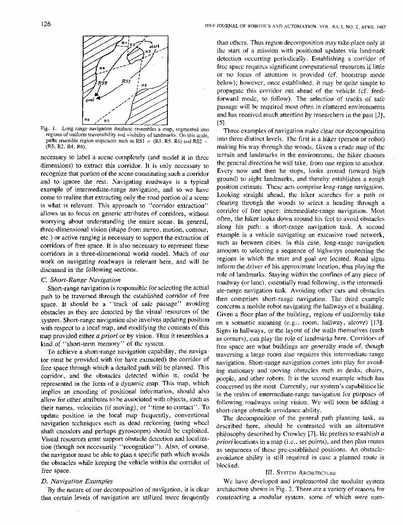
which to develop and test further navigational capabilities for planning at this level of resolution consists of establishing a autonomous vehicles. Experiments with parts of the system of which connect the and c4goal,, have been performed using the DARPA Autonomous regions. Thus the navigator must possess the computational Land Vehicle at Martin Marietta’s test site in Denver, CO. capabilities to construct such graphs and create region se-
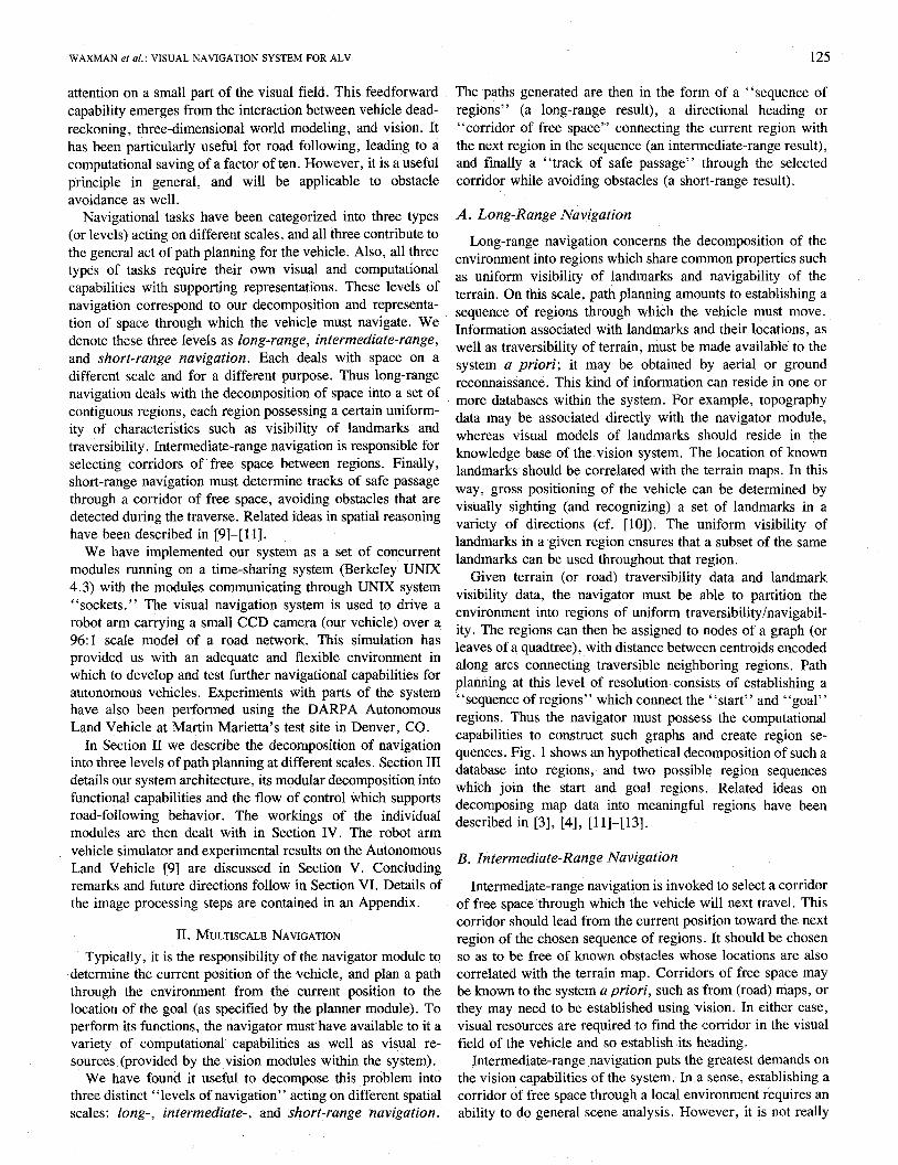
In Section I1 we describe the decomposition of navigation quences. Fig. shows an hypothetical decomposition of such a into three levels of path planning at different scales. Section 111 database into regions, and two possible region sequences details our system architecture, its modular decomposition into which join the start and goal regions. Related ideas on functional capabilities and the flow of control which supports decomposing map data into meaningful regions have been road-following behavior. The workings of the individual described in .[31, [41, [111-,131. modules are then dealt with in Section IV. The robot arm vehicle simulator and experimental results on the Autonomous Land Vehicle [9] are discussed in Section V. Concluding remarks and future directions follow in Section VI. Details of the image processing steps are contained in an Appendix.
II. MULTISCALE NAVIGATION Typically, it is the responsibility of the navigator module to
determine the current position of the vehicle, and plan a path through the environment from the current position to the location of the goal (as specified by the planner module). To perform its functions, the navigator must have available to it a variety of computational capabilities as well as visual re- sources (provided by the vision modules within the system).
We have found it useful to decompose this problem into three distinct “levels of navigation” acting on different spatial scales: long-, intermediate-, and short-range navigation.
B. Intermediate-Range Navigation
Intermediate-range navigation is invoked to select a corridor of free space through which the vehicle will next travel. This corridor should lead from the current position toward the next region of the chosen sequence of regions. It should be chosen so as to be free of known obstacles whose locations are also correlated with the terrain map. Corridors of free space may be known to the system apriori, such as from (road) maps, or they may need to be established using vision. In either case, visual resources are required to find the corridor in the visual field of the vehicle and so establish its heading.
Intermediate-range navigation puts the greatest demands on the vision capabilities of the system. In a sense, establishing a corridor of free space through a local environment requires an ability to do general scene analysis. However, it is not really
126 IEEE JOURNAL OF ROBOTICS AND AUTOMATION, VOL. RA-3, NO. 2. APRIL 1987
Fig. 1. Long-range navigation database resembles a map, segmented into regions of uniform traversibility and visibility of landmarks. On this scale, paths resemble region sequences such as RS1 = (R3, R5, R6) and RS2 = (R3, R2, R4, R6).
necessary to label a scene completely (and model it in three dimensions) to extract this corridor. It is only necessary to recognize that portion of the scene constituting such a corridor and to ignore the rest. Navigating roadways is a typical example of intermediate-range navigation, and so we have come to realize that extracting only the road portion of a scene is what is relevant. This approach to “corridor extraction” allows us to focus on generic attributes of corridors, without worrying about understanding the entire scene. In general, three-dimensional vision (shape from stereo, motion, contour, etc.) or active ranging is necessary to support the extraction of corridors of free space. It is also necessary to represent these corridors in a three-dimensional world model. Much of our work on navigating roadways is relevant here, and will be discussed in the following sections. C. Short-Range Navigation
Short-range navigation is responsible for selecting the actual path to be traversed through the established corridor of free space. It should be a “track of safe passage” avoiding obstacles as they are detected by the visual resources of the system. Short-range navigation also involves updating position with respect to a local map, and modifying the contents of this map provided either a priori or by vision. Thus it resembles a kind of “short-term memory” of the system.
To achieve a short-range navigation capability, the naviga- tor must be provided with (or have extracted) the corridor of free space through which a detailed path will be planned. This corridor, and the obstacles detected within it, could be represented in the form of a dynamic map. This map, which implies an encoding of positional information, should also allow for other attributes to be associated with objects, such as their names, velocities (if moving), or “time to contact”. TO update position in the local map frequently, conventional navigation techniques such as dead reckoning (using wheel shaft encoders and perhaps gyroscopes) should be exploited. Visual resources must support obstacle detection and localiza- tion (though not necessarily “recognition”). Also, of course, the navigator must be able to plan a specific path which avoids the obstacles while keeping the vehicle within the corridor of free space.
D. Navigation Examples By the nature of our decomposition of navigation, it is clear
that certain levels of navigation are utilized more frequently
than others. Thus region decomposition may take place only at the start of a mission with positional updates via landmark detection occurring periodically. Establishing a corridor of free space requires significant computational resources if little or no focus of attention is provided (cf. bootstrap mode below); however, once established, it may be quite simple to propagate this corridor out ahead of the vehicle (cf. feed- forward mode, to follow). The selection of tracks of safe passage will be required most often in cluttered environments and has received much attention by researchers in the past [2],
Three examples of navigation make clear our decomposition into three distinct levels. The first is a hiker (person or robot) making his way through the woods. Given a crude map of the terrain and landmarks in the environment, the hiker chooses the general direction he will take, from one region to another. Every now and then he stops, looks around (toward high ground) to sight landmarks, and thereby establishes a rough position estimate. These acts comprise long-range navigation. Looking straight ahead, the hiker searches for a path or clearing through the woods to select a heading through a corridor of free space: intermediate-range navigation. Most often, the hiker looks down around his feet to avoid obstacles along his path: a short-range navigation task. A second example is a vehicle navigating an extensive road network, such as between cities. In this case, long-range navigation amounts to selecting a sequence of highways connecting the regions in which the start and goal are located. Road signs inform the driver of his approximate location, thus playing the role of landmarks. Staying within the confines of any piece of roadway (or lane), essentially road following, is the intermedi- ate-range navigation task. Avoiding other cars and obstacles then comprises short-range navigation. The third example concerns a mobile robot navigating the hallways of a building. Given a floor plan of the building, regions of uniformity take on a semantic meaning (e.g., room, hallway, alcove) [131. Signs in hallways, or the layout of the walls themselves (such as corners), can play the role of landmarks here. Corridors of free space are what buildings are generally made of, though traversing a large room also requires this intermediate-range navigation. Short-range navigation comes into play for avoid- ing stationary and moving obstacles such as desks, chairs, people, and other robots. It is the second example which has concerned us the most. Currently, our system’s capabilities lie in the realm of intermediate-range navigation for purposes of following roadways using vision. We will soon be adding a short-range obstacle avoidance ability.
The decomposition of the general path planning task, as described here, should be contrasted with an alternative philosophy described by Crowley [7]. He prefers to establish a priori locations in a map (i.e., set points), and then plan routes as sequences of these pre-established positions. An obstacle- avoidance ability is still required in case a planned route is blocked.
111. SYSTEM ARCHITECTURE
PI.
We have developed and implemented the modular system architecture shown in Fig. 2. There are a variety of reasons for constructing a modular system, some of which were men-
WAXMAN et al.: VISUAL NAVIGATION SYSTEM FOR ALV
FEED-FORWARD MODES BOOTSTRAP AND.
ltnear features . gray segmentation . color analysis
127
I VISURL I RULES h MODELS road structures landmarks
GEOmETRY 3-0 SHAPE RECOVERY
contour / parallels . stereo monocular flow binocular flow active ranging
system control I 3-Dr.#.*
I I I 5 0 I 7 m n n m PILOT IlRVIGRTOR
goal speciftcation .I ”2~ +
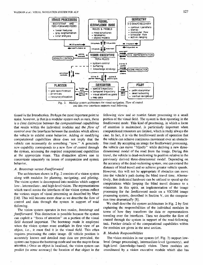
Fie. 2 . Modular system architecture for visual navigation. Flow of control
. inertial navigatlon map data resource allocation
. dead reckoning C . visual attentive goals +;:$= . priorltles
’lrn spatial trajectory temporal trajectory 4 I path Interpreter
* 0 \ I \
I
and dab over interfaces supports road following.
tioned in the Introduction. Perhaps the most important point to make, however, is that in a modular system such as ours, there is a clear distinction between the computational capabilities that reside within the individual modules and the flow of control over the interfaces between the modules which allows the vehicle to exhibit some behavior. Adding or modifying computational capabilities alone does not imply that the vehicle can necessarily do something “new.” A genuinely new capability corresponds to a new flow of control through the system, .accessing the required computational capabilities at the appropriate times. This distinction allows one to concentrate separately on issues of computation and system behavior.
A . Bootstrap versus Eeedforward The architecture shown in Fig. 2 consists of a vision system
along with modules for planning, navigating, and piloting. The vision system is decomposed into modules which support low-, intermediate-, and high-level vision. The representations which travel across the interfaces of the vision system reflect the various stages of visual processing as described by Marr [14]. This will become more clear as we describe the flow of control and data through the system in support of road following.
The vision system operates in two modes, bootstrap and feedforward. This distinction is possible because the system can exploit a ‘ ~ o c u s of attention” on a portion of the visual field deemed important. The bootstrap mode is employed when the vision system must establish its first view of an object, i.e., it must find it in the visual field. This often requires processing the entire image. (If vehicle position is accurately known and detailed map data are provided, the system can bypass the bootstrap mode and use the map to focus attention.) Once an object is localized, the vision system can predict (to some accuracy) the location of that object in the
foliowing view and so restrict future processing to a small poi-tion of the visual field. The system is then operating in the feedfonvard mode. This kind of processing, in which a focus of attention is maintained, is particularly important when computational resources are limited, which is really always the case. In fact, it is via the feedforward mode of operation that the vehicle can achieve continuous movement over an obstacle- free road. By accepting an image for feedfonvard processing, the vehicle can move “blindly” while deriving a new three- dimensional model of the road from the image, During this travel, the vehicle is dead-reckoning its position relative to the previously derived three-dimensional model. Depending on the accuracy of the dead-reckoning system, one can extend the distance of blind travel and so achieve greater vehicle speeds. However, this will not be appropriate if obstacles can move into the vehicle’s path during the blind travel time. Alterna- tively, fast dedicated hardware can be utilized to speed up the computations while keeping the blind travel distance to a minimum. In this spirit, an implementation of the image processing for the feedforward mode on a VICOM image processing system, described in Section V, cut the computa- tion time dramatically [SI.
We shall describe the system architecture in Fig. 2 by first explaining the responsibilities of the individual modules in terms of how they transform the data or representations traveling over the interfaces. Then we describe the flow of control through the system in support of the road-following task. Further details of the computational capabilities within the modules are given in the next section.
B. Module Responsibilities The vision modules in our system (cf. Fig. 2) support low-
level (image processing), intermediate-level (geometry), and high-level (knowledge-based) vision. These modules are coordinated by a vision executive module which also has
128 IEEE JOURNAL OF ROBOTICS AND AUTOMATION, VOL. RA-3, NO. 2, APRIL 1987
access to three-dimensional representation, scene prediction, and sensor control modules. The vision executive also supports interfaces to the planner and navigator modules. The pilot module communicates only with the navigator. These modules’ functional capabilities are listed inside each module in the diagram and are described in detail in the next subsection.
The vision system as a whole is responsible for perceiving objects of interest (e.g., roads and landmarks) and represent- ing them in an “object-centered’’ reference frame. The “image processing module” is responsible for extracting symbolic representations from the individual images. These image domain symbolics correspond to significant events in the signal data; they are general features which describe images (e.g., edges, lines, blobs). The transformation from TV signals to symbols represents an enormous reduction in data. This module constructs a representation akin to the “raw primal sketch” of Marr [14]. Extraction of symbols can be performed either on the entire image, or within a specified window. The module we call “visual knowledge base” has several responsibilities. Given the image domain symbolics extracted by the image processing module, the knowledge- based module tries to establish significant groupings of these symbols (e.g., pencils of lines). These groupings are global, corresponding to spatial organizations over large parts of the image, in contrast to the symbols themselves which are typically local groupings of events. This grouping process will then discard those symbols which are not found to belong to any group. This results in a representation similar to the “full primal sketch” of Marr [ 141. The visual knowledge base is also responsible for establishing meaningful groupings from three-dimensional representations provided by the ‘‘geometry module. ” Given the three-dimensional data, the knowledge- based module tries to recognize specific kinds of objects (e.g., roads), and so label important parts of the scene. The geometry module is responsible for three-dimensional shape recovery, converting the grouped symbolics (obtained earlier) into surface patches described in a viewer-centered reference frame, as in the “2.5-D sketch” of Marr [14]. The “vision executive” is the heart of the vision system; it maintains the “flow of control” through this part of the system, trying to meet the “attentive goals” (such as find road or find landmark or find obstacles) provided by the planner and navigator. It is this executive which triggers the mode of operation (bootstrap or feedforward). The vision executive is aided by several additional submodules which are also shown in Fig. 2 .
Once a three-dimensional model of the scene has been established in the viewer-centered coordinate system, it is converted to an object-centered representation by the “three- dimensional representation” module. This representation is more compact than the viewer-centered description, and corresponds to a world model organized around the static components of the scene which do, in fact, dominate the scene. In the case of “roads,” this is the representation passed to the navigator module for planning a path. This three- dimensional representation is also used by the “scene predic- tor” to focus attention on small areas of the visual field in
which important objects are located, even after the vehicle has traveled blind; it is the foundation upon which the feed- forward mode operates. Finally, the vision executive can control the pointing of the camera via a “sensor control” module. Thus, in seeking to find a landmark or road, for example, the executive establishes the visual field.
Three additional modules comprise our architecture as it currently stands. A “planner module” is responsible for establishing the overall goals of the system and assigning priorities to these goals. As we are concerned with navigation, these goals are typically location goals, either in a map or relative to something like a landmark located in a map. For “road following, ” a goal may be ‘‘move to point N on the road map.” It is also appropriate that the planner be responsible for overall resource allocation as this is where the “time sensitivity” of the system resides. Hence, priorities can be established and altered when deemed necessary. The “navigator module” is a special purpose planning module. It is responsible for generalizea path planning, as described in Section 11. The navigator must also track the position of the vehicle through the three-dimensional representation as it moves blindly, using “travel” data from the pilot. Once the navigator establishes a particular path for some short distance, it passes the path to the pilot module which interprets this path into steering and motion commands for the vehicle. The pilot is also responsible for monitoring the dead-reckoning (and inertial navigation) unit aboard the vehicle. It should convert wheel shaft encoder readings and gyroscope headings into directional travel since the last time “travel” was requested by the navigator.
C. Road-Following By accessing the computational capabilities which reside in
the modules in a particular order, the system can exhibit certain behaviors. Thus, in a modular system, the flow of control through the system plays a central role. In Fig. 2 we have indicated the flow of control between modules which supports the road-following task. Beginning with the vehicle at a standstill and the road somewhere in the visual field, the planner specifies the goal to reach some point or distance down the road. This location goal is passed to the navigator which must specify the visual attentive goal of “find the road in the field of view,” passing it to the vision executive. The vision system must first find the road and so the bootstrap mode of processing is selected, and an image is accepted into the image processing module. The executive also selects which image processing procedure should be utilized; we currently use ‘‘linear feature extraction,” cf. Appendix. Linear features which dominate the scene (are expected to reflect road boundaries and markings, and so on) comprise two-dimensional symbolics passed back to the executive in the form of endpoints of each feature. These symbols are then passed to the knowledge base where they are grouped into pencils of lines. A road with turns or changes in slope in the field of view will give rise to several pencils in the same image. The pencils are then returned to the executive where they are then interpreted one at a time, from bottom to top of the image (corresponding to “near to far” in the world). Each pencil is
WAXMAN et al.: VISUAL NAVIGATION SYSTEM FOR ALV 129
passed to the geometry module where it is given a three- dimensional shape interpretation in the form of parallel lines on a planar surface patch. This is essentially “shape from contour”; it is capable of recovering road geometry over rolling terrain (cf. Section IV). Thus the two-dimensional pencils of lines are converted to three-dimensional parallels which are relayed to the knowledge base via the executive. As each set of parallels arrives in the knowledge base, general knowledge about road structures is used to decide if the parallels and corresponding surface patch “make sense.” If not, alternate groupings of lines are considered. (A more mature system would utilize a variety of symbolic descrip- tions,, fusing them with knowledge to interpret the scene.) Each successive pencil, interpreted as parallels, is checked for consistency with already accepted parallels, thereby building up a viewer-centered three-dimensional description of the road. Parts of the road are labeled as “boundaries, center line, lane markers, or shoulder boundaries.” That is, the object “road” is recognized via its attributes in the world, particularly their spatial relations. This scene model is then passed to the three-dimensional representation module which converts the viewer-centered model of the road (consisting of a sequence of parallel lines in space relative to the camera) into a compact object-centered representation in which each planar patch is described relative to the previous patch, and the road width and number of lanes is specified. The vehicle is then located relative to the first planar patch. Before passing this represen- tation on to the navigator (the vehicle still has not moved), the executive uses the. scene predictor to select small windows near the bottom of the visual field inside of which the left and right road boundaries are located. The executive then utilizes the local image processing of the feedforwaid mode to refine the locations of the road boundaries (cf. Appendix). Once the road boundaries have been established, the system tries to continue to track them through the image domain, checking their three-dimensional interpretations for consistency with the rules. Once the road is extracted from the first image, and its boundaries have been refined giving rise to a more accurate three-dimensional representation, this representation is passed on to the navigator. (This road map can be pasted on to a map of a previous segment of road and passed to the planner for future use.) The navigator then plans a path down the road and passes segments of this path to the pilot. The pilot decomposes the path into motion commands, and the vehicle begins to move. Periodically, the pilot returns the distance and heading actudly traveled to the navigator. The navigator informs the vision executive of position and the executive requests that a new image be taken. The executive also passes this position to the scene predictor which, utilizing the previous three-dimen- sional representation, determines the appearance of the road boundaries from this new vantage point and selects new windows near the bottom of the new image inside of which the road boundaries are to be found. The new image is then processed in the feedforward mode and the system continues on in this way until instructed to stop. In this manner, the vehicle travels over road segments about 10 m long using a map it created from an image taken some 10 m ahead of that segment, maintaining a continuous motion.’
We should point out that the size of the visual field used for focusing attention in the feedforward mode reflects the uncertainty in the position and heading of the vehicle as determined by the dead-reckoning system as well as uncer- tainty in .camera pointing. Mainly, it must accommodate uncertainties in the visually constructed road map. A 5 O x 5 O window would be appropriate given a positional error of about 0.3 m and a pointing error of l o with respect to the road boundaries [ 11.
IV. COMPUTATIONAL CAPABILITIES OF MODULES Having described the nature of the responsibilities assigned
to the individual modules, as well as how they are linked by a flow of control to support the task of road-following, we now turn to the specific computations that take place within the modules. The nature of these computations is suggested by the points listed within the module boxes of Fig. 2. Some of the capabilities shown in the diagram are not yet installed in our system, though they are suggested by the modular decomposi- tion itself and their relation to currently existing capabilities. We consider each module separately.
A . Image Processing We have developed algorithms for the extraction of domi-
nant linear features from entire (gray level) images as well as gray and color segmentation routines. These analyses provide independent representations of the information contained in the images in the form of boundary-based and region-based descriptions, respectively. These routines are relevant to the bootstrap mode of processing described earlier. Related versions were also developed to support the feedforward mode. Examples of this processing on a road image are shown in Figs. 3 and 4. A detailed description of the image processing steps is included in the Appendix. The capabilities we have already installed combine low-level operations with certain grouping procedures to derive particular symbolic descriptors. Thus our linear feature detector relies on the grouping of pixels with similar gradient orientation, yielding a linear feature with global support (and poor localization) in the bootstrap mode and one with local support (and good localization) in the feedforward mode. The segmentation procedures are based on edge-preserving smoothing followed by a connected-components analysis. The color version of the segmentation procedure is far less sensitive to parameters than is the gray version. (It also provides the additional measure of “color” for each segment.) Linear feature extraction is completely automatic. Since the knowledge-based reasoning module in our system cannot currently fuse multiple sources of data (such as both linear features and regions), we utilize only the linear features when running the entire system. More details on the color segmentation algorithm can be found in [151.
B. Visual Knowledge Base This module implements two separate vision tasks-seeking
significant groupings of symbols derived from an image and checking consistency of three-dimensional shape recovery with generic models of objects (e.g. , roads). Many types of
130 IEEE JOURNAL OF ROBOTICS AND AUTOMATION, VOL. RA-3, NO. 2, APRIL 1987
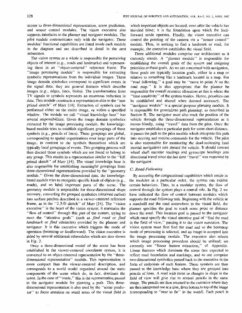
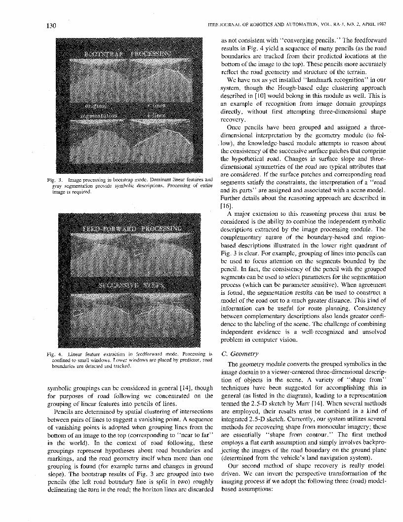
Fig. 3. Image processing in bootstrap mode. Dominant linear features and gray segmentation provide symbolic descriptions. Processing of entire image is required.
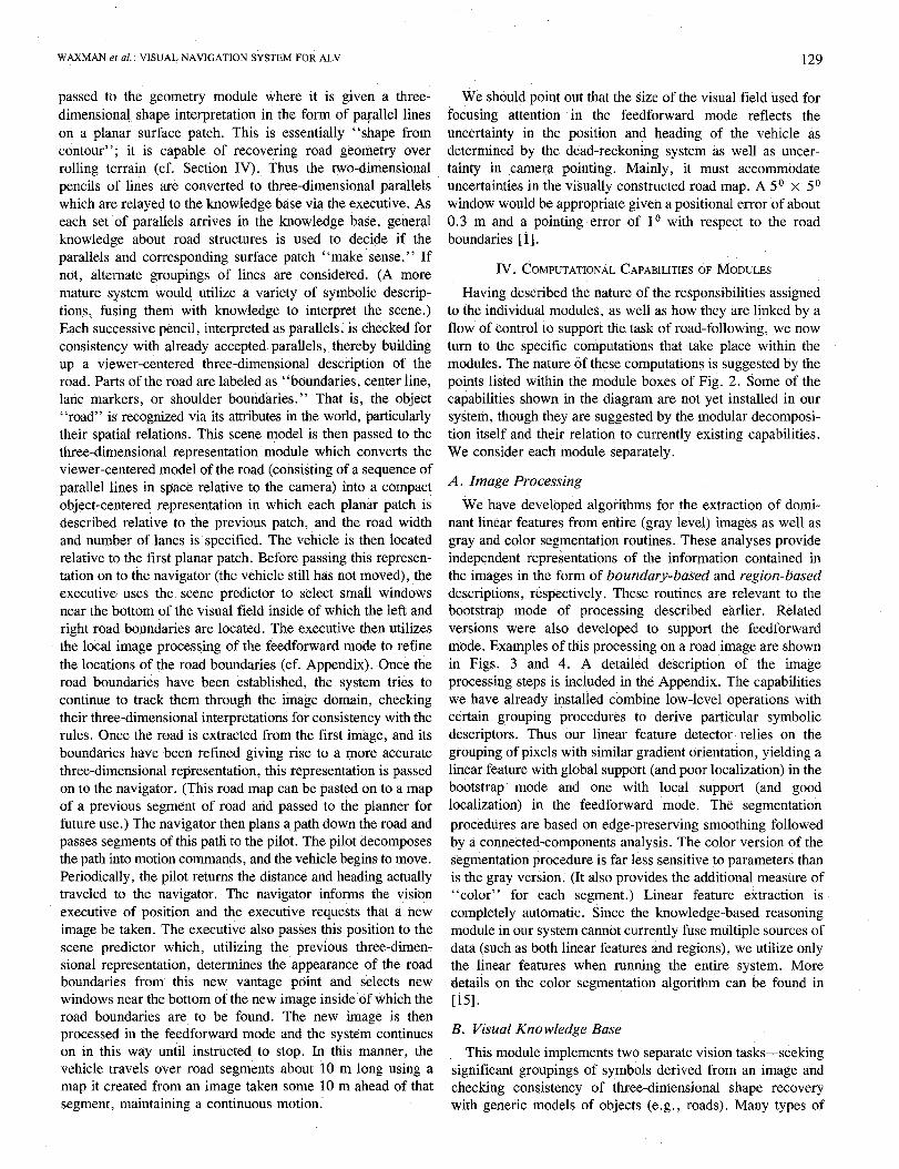
Fig. 4. Linear feature extraction in feedforward mode. Processing is confined to small windows. Lower windows are placed by predictor, road boundaries are detected and tracked.
symbolic groupings can be considered in general [ 141, though for purposes of road following we concentrated on the grouping of linear features into pencils of lines.
Pencils are determined by spatial clustering of intersections between pairs of lines to suggest a vanishing point. A sequence of vanishing points is adopted when grouping lines from the bottom of an image to the top (corresponding to “near to far” in the world). In the context of road following, these groupings represent hypotheses about road boundaries and markings, and the road geometry itself when more than one grouping is found (for example turns and changes in ground slope). The bootstrap results of Fig. 3 are grouped into two pencils (the left road boundary line is split in two) roughly delineating the turn in the road; the horizon lines are discarded
as not consistent with “converging pencils.” The feedforward results in Fig. 4 yield a sequence of many pencils (as the road boundaries are tracked from their predicted locations at the bottom of the image to the top). These pencils more accurately reflect the road geometry and structure of the terrain.
We have not as yet installed “landmark recognition” in our system, though the Hough-based edge clustering approach described in [lo] would belong in this module as well. This is an example of recognition from image domain groupings directly, without first attempting three-dimensional shape recovery.
Once pencils have been grouped and assigned a three- dimensional interpretation by the geometry module (to fol- low), the knowledge-based module attempts to reason about the consistency of the successive surface patches that comprise the hypothetical road. Changes in surface slope and three- dimensional symmetries of the road are typical attributes that are considered. If the surface patches and corresponding road segments satisfy the constraints, the interpretation of a “road and its parts” are assigned and associated with a scene model. Further details about the reasoning approach are described in U61.
A major extension to this reasoning process that must be considered is the ability to combine the independent symbolic descriptions extracted by the image processing module. The complementary nature of the boundary-based and region- based descriptions illustrated in the lower right quadrant of Fig. 3 is clear. For example, grouping of lines into pencils can be used to focus attention on the segments bounded by the pencil. In fact, the consistency of the pencil with the grouped segments can be used to select parameters for the segmentation process (which can be parameter sensitive). When agreement is found, the segmentation results can be used to construct a model of the road out to a much greater distance. This kind of information can be useful for route planning. Consistency between complementary descriptions also lends greater confi- dence to the labeling of the scene. The challenge of combining independent evidence is a well-recognized and unsolved problem in computer vision.
C. Geometry The geometry module converts the grouped symbolics in the
image domain to a viewer-centered three-dimensional descrip- tion of objects in the scene. A variety of “shape from” techniques have been suggested for accomplishing this in general (as listed in the diagram), leading to a representation termed the 2.5-D sketch by Marr [14]. When several methods are employed, their results must be combined in a kind of integrated 2.5-D sketch. Currently, our system utilizes several methods for recovering shape from monocular imagery; these are essentially “shape from contour.” The first method employs a flat earth assumption and simply involves backpro- jecting the images of the road boundary on the ground plane (determined from the vehicle’s land navigation system).
Our second method of shape recovery is really model- driven. We can invert the perspective transformation of the imaging process if we adopt the following three (road) model- based assumptions:
WAXMAN et al.: VISUAL NAVIGATION SYSTEM FOR ALV 131
1) pencils in the image domain correspond to planar
2) continuity in the image domain implies continuity in the
3) the camera sits above the first visible ground plane (at
parallels in the world;
world;
the bottom of the image).
Our three-dimensional reconstruction will then characterize a road of constant width, with turns and changes in slope and bank. The reconstruction process amounts to an integration out from beneath the vehicle off into the distance, along local parallels over topography modeled as a sequence of planar surface patches.
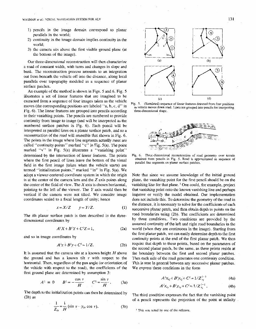
An example of the method is shown in Figs. 5 and 6. Fig. 5 illustrates a set of linear features that are imagined to be extracted from a sequence of four images taken as the vehicle moves (the corresponding positions are labeled “a, b, c, d” in Fig. 6 ) . The linear features are grouped into pencils according to their vanishing points. The pencils are numbered to provide continuity from image to image (and will be interpreted as the numbered surface patches in Fig. 6). Each pencil will be interpreted as parallel lines on a planar surface patch, and so a reconstruction of the road will resemble that shown in Fig. 6. The points in the image where line segments actually meet are called “continuity points” marked “c” in Fig. 5(a). The point marked “v” in Fig. 5(a) illustrates a “vanishing point” determined by the intersection of linear features. The points where the first pencil of lines leave the bottom of the visual field in the first image (taken when the vehicle starts) are termed “initialization points,” marked “in” in Fig. 5(a). We adopt a viewer-centered coordinate system in which the origin is at the center of the camera lens and the Z axis points along the center of the field of view. The X axis is chosen horizontal, pointing to the left of the viewer. The Y axis would then be vertical if the camera were not tilted. We consider image coordinates scaled to a focal length of unity; hence
x=x/z y = Y/Z. (1)
The ith planar surface patch is then described in the three- dimensional coordinates by
A’X+B’Y+C’Z= I , ( W
and so in image coordinates by
A‘xiB‘y+C’= 1/z. (2b)
It is assumed that the camera sits at a known height H above the ground and has a known tilt 7 with respect to the horizontal. Then, regardless of the pan angle (or orientation of the vehicle with respect to the road), the coefficients of the first ground plane are determined by assumption 3:
The depth to the initialization points can then be determined by (2b) as
Fig. 5 . (Simulated) sequence of linear features detected from four positions as vehicle moves down road. Lines are grouped into pencils for interpreting three-dimensional shape.
Fig. 6. Three-dimensional reconstruction of road geometry over terrain obtained from pencils in Fig. 5 . Road is approximated as sequence of parallel line segments on planar surface patches.
Note that since we assume knowledge of the initial ground plane, the vanishing point for the first pencil should be on the vanishing line for that plane. One could, for example, project that vanishing point onto the known vanishing line and perhaps improve or verify the model obtained. Our implementation does not include this. To determine the geometry of the road in the distance, it is necessary to solve for the coefficients of each successive planar patch, and then obtain depth to points on the road boundaries using (2b). The coefficients are determined by three conditions. Two conditions are provided by the assumed continuity of the left and right road boundaries in the world (when they are continuous in the image). Starting from the first planar patch, we can easily determine depth to the first continuity points at the end of the first planar patch. We then require that depth to these points, based on the parameters of the second planar patch, be the same, as these points reside at the boundary between the first and second planar patches. Thus each side of the road generates one continuity condition. This is true in general between any successive planar patches. We express these conditions in the form
The third condition expresses the fact that the vanishing point of a pencil represents the projection of the point at infinity
.,. ’ This was noted by one of the referees.
132 IEEE JOURNAL OF ROBOTICS AND AUTOMATION, VOL. RA-3, NO. 2, APRIL 1987
(i.e., Z a):
A iXUi + B’& + C‘= 0. (4c)
Equations (4a)-(4c) form a set of three linear equations in the three unknown coefficients describing the ith planar patch. Thus starting from the first ground plane, one works outward from the vehicle, building a model of the road topography in the viewer-centered coordinate system.
The geometry module can utilize this method of reconstruct- ing road topography. As each planar patch is recovered, the linear features are subdivided into segments which are physically opposite each other on the road in three dimensions. This simplifies the symmetry checks imposed by the visual knowledge base following shape recovery and is also required for the predictor. Clearly, this method of shape recovery is tightly coupled to the hypothesis that the pencils of lines correspond to road boundaries and markings. The hypothesis itself, however, is generated following the grouping operation. That is, the “shape from” process is being imposed with a particular generic object in mind.
However, we encountered some problems with this shape recovery algorithm. On curves in roads, for example, the linear segments extracted by the image processing do not correspond to parallel road segments, and the constructed road model was incorrect. An alternative, which our system currently employs, is to employ a flat earth model on curved road segments using the planar facet from the last straight segment to define the “flat earth.” We have also developed another monocular inverse perspective algorithm for constant- width zero-bank roads that appears to be very robust. See Dementhon [17] for a detailed description of this algorithm.
D. Vision Executive This module does not really perform any computations as
yet. It maintains the flow of control through the system to exhibit a behavior, such as road following. As the contents of the knowledge base are expanded to incorporate other object models, the vision executive will have to make decisions about what scene features to search for, which sensors to use in those searches, etc. Once the system modules are mapped to individual nodes of a multiprocessor such as the Butterfly, the vision executive will be required to buffer messages between modules as the computations are asynchronous.
E. Three-Dimensional Representation This module converts the three-dimensional viewer-cen-
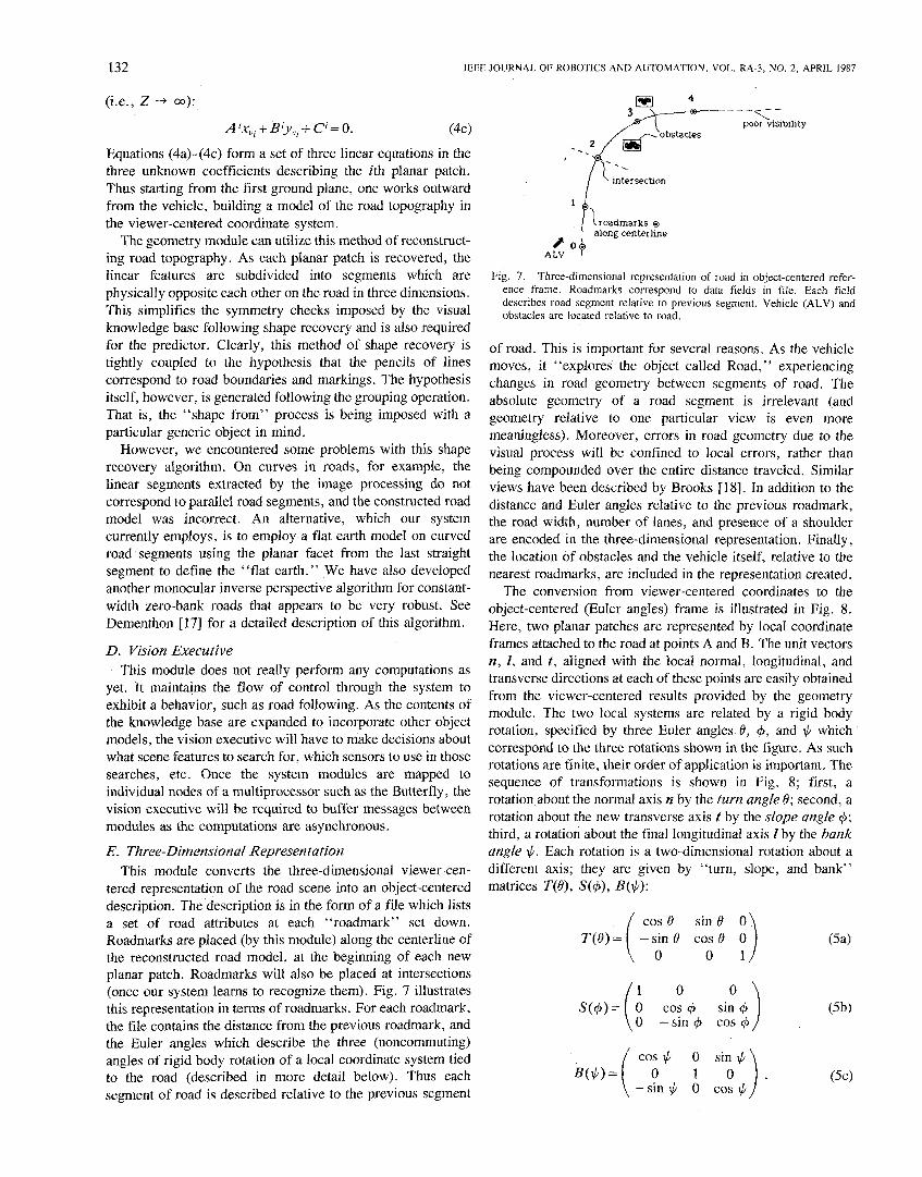
tered representation of the road scene into an object-centered description. The description is in the form of a file which lists a set of road attributes at each “roadmark” set down. Roadmarks are placed (by this module) along the centerline of the reconstructed road model, at the beginning of each new planar patch. Roadmarks will also be placed at intersections (once our system learns to recognize them). Fig. 7 illustrates this representation in terms of roadmarks. For each roadmark. the file contains the distance from the previous roadmark, and the Euler angles which describe the three (noncommuting) angles of rigid body rotation of a local coordinate system tied to the road (described in more detail below). Thus each segment of road is described relative to the previous segment
---x-- poor visiblllty
1
along centerline roadmarks o
A LV
Fig. 7. Three-dimensional representation of road in object-centered refer- ence frame. Roadmarks correspond to data fields in file. Each field describes road segment relative to previous segment. Vehicle (ALV) and obstacles are located relative to road.
of road. This is important for several reasons. As the vehicle moves, it “explores the object called Road,” experiencing changes in road geometry between segments of road. The absolute geometry of a road segment is irrelevant (and geometry relative to one particular view is even more meaningless). Moreover, errors in road geometry due to the visual process will be confined to local errors, rather than being compounded over the entire distance traveled. Similar views have been described by Brooks [18]. In addition to the distance and Euler angles relative to the previous roadmark, the road wi&ch, number of lanes, and presence of a shoulder are encoded in the three-dimensional representation. Finally, the location of obstacles and the vehicle itself, relative to the nearest roadmarks, are included in the representation created.
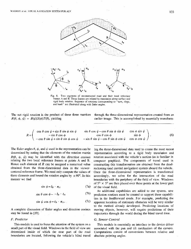
The conversion from viewer-centered coordinates to the object-centered (Euler angles) frame is illustrated in Fig. 8. Here, two planar patches are represented by local coordinate frames attached to the road at points A and B. The unit vectors n, I , and t , aligned with the local normal, longitudinal, and transverse directions at each of these points are easily obtained from the viewer-centered results provided by the geometry module. The two local systems are related by a rigid body rotation, specified by three Euler angles. 0, 4, and + which correspond to the three rotations shown in the figure. As such rotations are finite, their order of application is important. The sequence of transformations is shown in Fig. 8; first, a rotation about the normal axis n by the turn angle 0; second, a rotation about the new transverse axis t by the slope angle 4; third, a rotation about the final longitudinal axis I by the bank angle $. Each rotation is a two-dimensional rotation about a different axis; they are given by “turn, slope, and bank” matrices T(0), S ( 4 ) , B(#):
1 0 0 cos 4 sin 4 0 -sin r$ cos 4
COS $ 0 sin $
-sin $ 0 cos # i B(+)= 0 1
WAXMAN et al.: VISUAL NAVIGATION SYSTEM FOR ALV 133
Fig. 8. Two segments of reconstructed road and their local reference frames A and B. These frames are related by translation along surface and rigid body rotation. Sequence of rotations corresponding to “turn, slope, and bank” are illustrated along with Euler angles.
The net rigid rotation is the product of these three matrices through the three-dimensional representation created from an R(0, 9, $1 = B($)S(+)T(@, yielding earlier image. This is accomplished by essentially transform-
cos 0 cos $ + sin 0 sin + sin $ sin 0 cos $ - cos 0 sin + sin $ cos 4 sin $
-cos 0 sin $+sin 0 sin + cos $ -sin 0 sin $-cos 0 sin + cos $ cos + cos $ R = ( - sin 0 cos + cos 0 cos + sin 9 (6)
The Euler angles 0, 9, and $ used in the representation can be determined by noting that the elements of the rotation matrix R(0, +, $) may be identified with the direction cosines relating the two local reference frames at points A and B. Hence each element of R can be assigned a numerical value obtained from the three-dimensional data in the viewer- centered reference frame. We need only compute the values of three elements and bound the rotation angles by k 90°. In this manner we find
A complete discussion of Euler angles and direction cosines may be found in [ 191.
F. Predictor This module is used to focus the attention of the system on a
small part of the visual field. Windows in the field of view are determined inside of which the near part of the road boundaries are located, following the vehicle’s blind travel
ing the three-dimensional data used to create the most recent representation according to a rigid body translation and rotation associated with the vehicle’s motion (as is familiar in computer graphics). The components of travel used in constructing this transformation are obtained from the dead- reckoning (and inertial navigation) system aboard the vehicle. Once the three-dimensional representation is transformed accordingly, we solve for the intersection of the road boundaries with the periphery of the field of view. Windows of 5 O X S o are then placed over these points at the lower part of the visual field.
As additional capabilities are added to our system, new prediction routines must be created to support these capabili- ties in the feedforward mode. For example, predicting the apparent locations of stationary obstacles will be very similar to the method already developed. Predicting locations of moving objects, however, will require predictions of their trajectories through the world during the blind travel time.
G. Sensor Control This module is essentially an interface to the device driver
associated with the pan and tilt mechanism of the camera. Computations consist of conversions between relative and absolute pointing angles.
134 IEEE JOURNAL OF ROBOTICS AND AUTOMATION, VOL. RA-3, NO. 2, APRIL 1987
H. Navigator This module must provide computational capabilities in
support of generalized path planning, as described in Section 11. Thus it must be able to establish vehicle position from known landmarks sighted, generate region graphs from visibility/traversibility data, generate region sequences be- tween current position and goal, and plan paths down corridors of free space while avoiding obstacles. Our current navigator is specific to following obstacle-free roads (corri- dors), and so path planning consists of smoothly changing the heading of the vehicle in accordance with the three-dimen- ’ sional representation derived from the visual process. This is accomplished by computing cubic arcs as asymptotic paths. Given the current position and orientation of the vehicle, a cubic arc is derived which begins at the vehicle, slopes in the direction of vehicle heading, and terminates 13 m along the road centerline, in the direction of the centerline. This cubic arc is used as a path for the next 3 m (about one vehicle length) at which point a new cubic arc is derived which terminates another 13 m ahead. That is, the vehicle is always steered towards a point which is 13 m ahead of it, along the centerline. Thus the vehicle’s path will be asymptotic to the road centerline. (If the road has more than one lane, we displace the centerline to the middle of a lane.) This yields paths with smooth changes in heading. When obstacles are introduced onto the road, we must adjust the termination point of a cubic arc so that no part of the arc intersects an obstacle nor crosses the road boundary.
In addition to planning spatial trajectories, the navigator must plan temporal ones as well, essentially adjusting the speed of the vehicle in accordance with the upcoming demands of the road geometry. As our vision system generates a model of the road to quite far ahead of the vehicle, the navigator should be able to perform simple rule-based reasoning about speed. Thus the vehicle could speed up on straightaways, and slow down on turns. We currently operate at a single vehicle speed.
To support the focus of attention mechanism in the feedforward mode, the navigator must track vehicle position through the three-dimensional representation in response to. dead-reckoning data provided by the pilot. This information is made available to the vision executive at its request. This is currently implemented in our system. I. Pilot
This module converts the cubic arcs obtained from the navigator into a sequence of conventional steering commands used over the next 3 m. They decompose a curved >,ath into a set of short straight line segments. These motion commands must then interface to the motor controls of the vehicle. (In our case, the interface is to the motion control software of a robot arm, as described in the next section.) The pilot is also responsible for sending dead-reckoning data from the vehicle to the navigator. The pilot converts the raw data into measured travel and returns this information to the navigator several times per second. J. Planner
Our current planner is quite simple; it merely specifies a “distance goal,” e.g., move to the point 60 m further down
the road. A mature planning module could have arbitrary complexity, specifying high-level navigation goals, assigning priorities to these goals, monitoring progress as a function of time, and constructing contingency plans. It would also be responsible for allocating computational resources throughout the system. However, until the vehicle can exhibit a variety of behaviors, it seems rather premature to concentrate on issues of high-level planning.
v. LABORATORY SIMULATION AND EXPERIMENTS
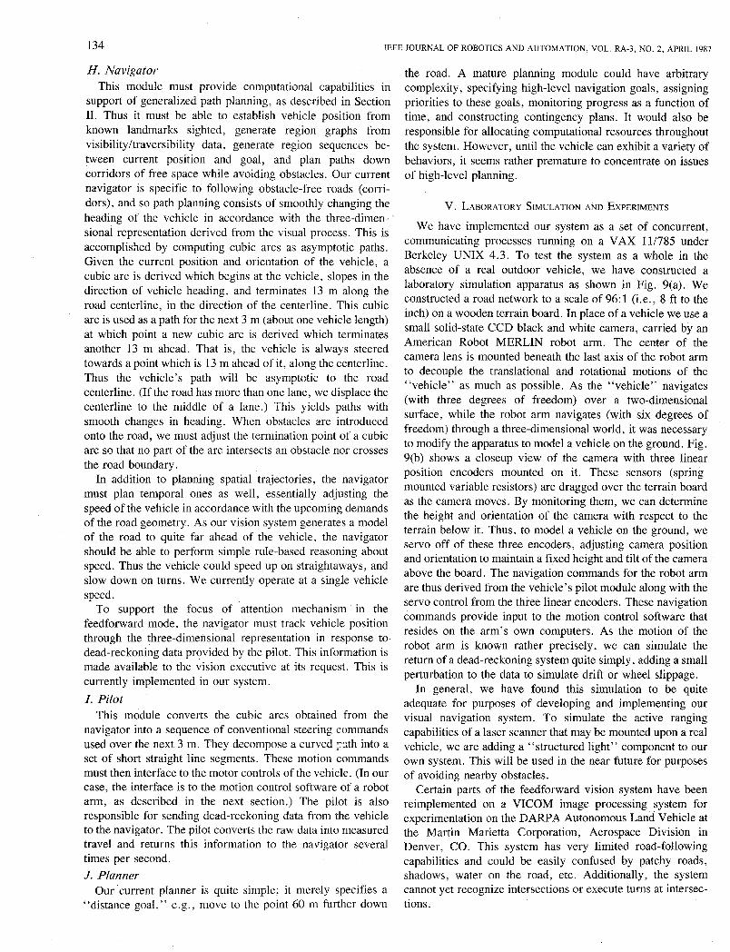
We have implemented our system as a set of concurrent, communicating processes running on a VAX 11 178.5 under Berkeley UNIX 4.3. To test the system as a whole in the absence of a real outdoor vehicle, we have constructed a laboratory simulation apparatus as shown in Fig. 9(a). We constructed a road network to a scale of 96:l (i.e., 8 ft to the inch) on a wooden terrain board. In place of a vehicle we use a small solid-state CCD black and white camera, carried by an American Robot MERLIN robot arm. The center of the camera lens is mounted beneath the last axis of the robot arm to decouple the translational and rotational motions of the “vehicle” as much as possible. As the “vehicle” navigates (with three degrees of freedom) over a two-dimensional surface, while the robot arm navigates (with six degrees of freedom) through a three-dimensional world, it was necessary to modify the apparatus to model a vehicle on the ground. Fig. 9(b) shows a closeup view of the camera with three linear position encoders mounted on it. These sensors (spring- mounted variable resistors) are dragged over the terrain board as the camera moves. By monitoring them, we can determine the height and orientation of the camera with respect to the terrain below it. Thus, to model a vehicle on the ground, we servo off of these three encoders, adjusting camera position and orientation to maintain a fixed height and tilt of the camera above the board. The navigation commands for the robot arm are thus derived from the vehicle’s pilot module along with the servo control from the three linear encoders. These navigation commands provide input to the motion control software that resides on the arm’s own computers. As the motion of the robot arm is known rather precisely, we can simulate the return of a dead-reckoning system quite simply, adding a small perturbation to the data to simulate drift or wheel slippage.
In general, we have found this simulation to be quite adequate for purposes of developing and implementing our visual navigation system. To simulate the active ranging capabilities of a laser scanner that may be mounted upon a real vehicle, we are adding a “structured light” component to our own system. This will be used in the near future for purposes of avoiding nearby obstacles.
Certain parts of the feedforward vision system have been reimplemented on a VICOM image processing system for experimentation on the DARPA Autonomous Land Vehicle at the Martin Marietta Corporation, Aerospace Division in Denver, CO. This system has very limited road-following capabilities and could be easily confused by patchy roads, shadows, water on the road, etc. Additionally, the system cannot yet recognize intersections or execute turns at intersec- tions.
WAXMAN et ai.: VISUAL NAVIGATION SYSTEM FOR ALV 135
(b) Fig. 9. ALV simulation apparatus. (a) Mini-CCD camera is carried over
terrain board by robot arm, road network is scaled by 96: 1. (b) Three linear position encoders are mounted to camera and touch board, they are used to adjust camera height and orientation.
Using 48-by-32 first windows and 32-by-32 subsequent windows on Denver test-track vehicle images, processing typically takes 6-7 s of microprocessor and pipelined-image- processor time, including approximately 2.5 s for the first two and 1.5 s for the subsequent windows’ processing time. This system was used to drive the ALV over several hundred meters of the Martin Marietta test track in November 1985 at a speed of 3 km/h. This involved computing sufficiently accurate road models from 20 consecutive frames. Note that neither the predictor nor the sensor control modules were included in this implementation. This not only reduced the speed at which the vehicle could operate (since the initial windows were unnecessarily large), but also reduced the overall reliability of the system. An additional set of experi- ments was conducted in August 1986 with a much more complete vision implementation.
VI. CONCLUDING REMARKS We have developed our first generation visual navigation
system capable of navigating on roadways at about 3 kmlh. Motivated by this application, a more general modular system architecture was created in which “computational capabili- ties” and “flow of control” play distinct roles. Our system runs as a set of concurrent processes communicating with each other in a manner that resembles distributed computing. Thus
it will be rather easy to map our system onto such multiproces- sors. We are, in fact, currently developing a version of our vision system on a 16 processor Butterfly parallel processing system [20]. Image preprocessing (smoothing, edge detection, etc.) is still performed on the VICOM, but the Hough transforms, predictor, window placement, and inverse per- spective modules will all run on the Butterfly. Puri and Davis [21] contains a detailed description of this system.
Many extensions are pianned for our system, such as stereo vision in the geometry module, reasoning about multiple sources of data (linear features and segmented regions) in the visual knowledge base, and planning paths around obstacles and through road networks in the navigator module. To support such extensions, we have built a structured light range sensor that mounts on the robot arm and can be carried across the terrain board, The design and construction of this sensor is described in Dementhon [22]. We have also developed a set of simple road obstacle detection algorithms for range data based on comparing observed derivatives of range data to expected derivatives of range data. These algorithms are discussed in Veatch and Davis [23].
A map of our terrain board has been constructed, and it will be used by the vision executive to predict important visual events such as road intersections and changes in structure, e.g., road width or road composition. This map will be similar in structure, scale, and content to the map developed by the Army’s Engineer Topographic Laboratory for the Martin Marietta test site. The modularity of our system should make the incorporation of such map information relatively straight- forward. The image processing module has been enhanced to include other road boundary detection algorithms. For exam- ple, we have recently had success with a local segmentation algorithm that adaptively thresholds each window, in the feedforward mode, based on sampling the road intensities in that window. Details of this algorithm and other modifications to the image processing module are presented in Kushner and Davis [24].
APPENDIX IMAGE PROCESSING ALGORITHMS
A . Bootstrap Image Processing When the ALV begins its road-following task, as no
information is usually available about where the vehicle is with respect to the road, it must process the entire image to construct a model of the visible portion of road, in the world domain. This is the bootstrap phase.
1) Linear Feature Extraction: We have developed image processing algorithms which extract the dominant linear features in the imagery under the assumption that roadways generate such features in a scene. We are not interested in all the linear features in a scene, only the dominant ones. These features are usually correlated with road boundaries, mark- ings, and shoulders, all of which are important for navigating on roads.
In both modes, bootstrap and feedforward, the extraction of linear features is the result of a sequence of image processing steps including smoothing, gradient, extraction of dominant directions, and Hough transformation to find the line segments
136 IEEE JOURNAL OF ROBOTICS AND AUTOMATION, VOL. RA-3, NO. 2, APRIL 1987
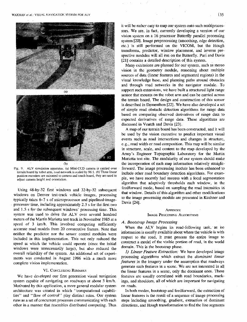
(c) (dl Fig. 10. Bootstrap image processing steps for linear feature extraction. (a) Original image. (b) Upper left: Sobel gradient
magnitude. Upper right: Sobel gradient direction. Lower left: results of linear enhancement. Lower right: weighted histogram of the direction image. (c) Points in original image corresponding to strongest four peaks. (d) Points which survived shrinking and expanding.
corresponding to these principal directions. For the bootstrap mode, we describe these steps in more detail in the context of the example, "bending road," as illustrated in Fig. 10.
The various processing steps applied over the image are as follows.
1) The original image is shown in Fig. 10(a). This is a 256 x 256 6-bit gray level image. The image is first blurred to reduce the noise, by performing a local average in a 5 X 5 neighborhood.
2) The Sobel operator is then applied to obtain the gradient magnitude and direction at each pixel. The magnitude of the gradient, encoded in gray, is shown in the upper left quadrant of Fig. 10(b). The upper right quadrant of the same picture shows the distribution of directions of the gradient vector (encoded in gray) wherever the magnitude exceeded a very low threshold (to remove regions of constant gray level from
consideration). Dominant linear features in the original corres- pond to long features of constant gray level in this direction picture.
3) The next step is to enhance the linear features in the image. Our enhancement method utilizes the gradient orienta- tion as the dominant measure. The strength of an edge depends upon the edge orientations of neighboring pixels: this is the notion of "local support." For a measure of this IocaI support, we first choose a neighborhood around the considered pixel: it is a rectangular window centered around this pixel, oriented approximately in the same direction as the center pixel gradient direction. A count is then calcuiated and assigned to the center pixel. Each pixel within the window contributes either a 0 or 1 to the count:
0 if the direction of an outer pixel is within 15" of the value
WAXMAN et ai.: VISUAL NAVIGATION SYSTEM FOR ALV
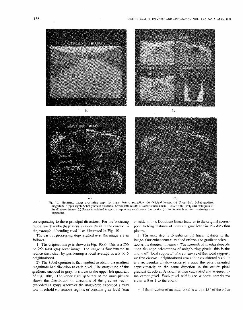
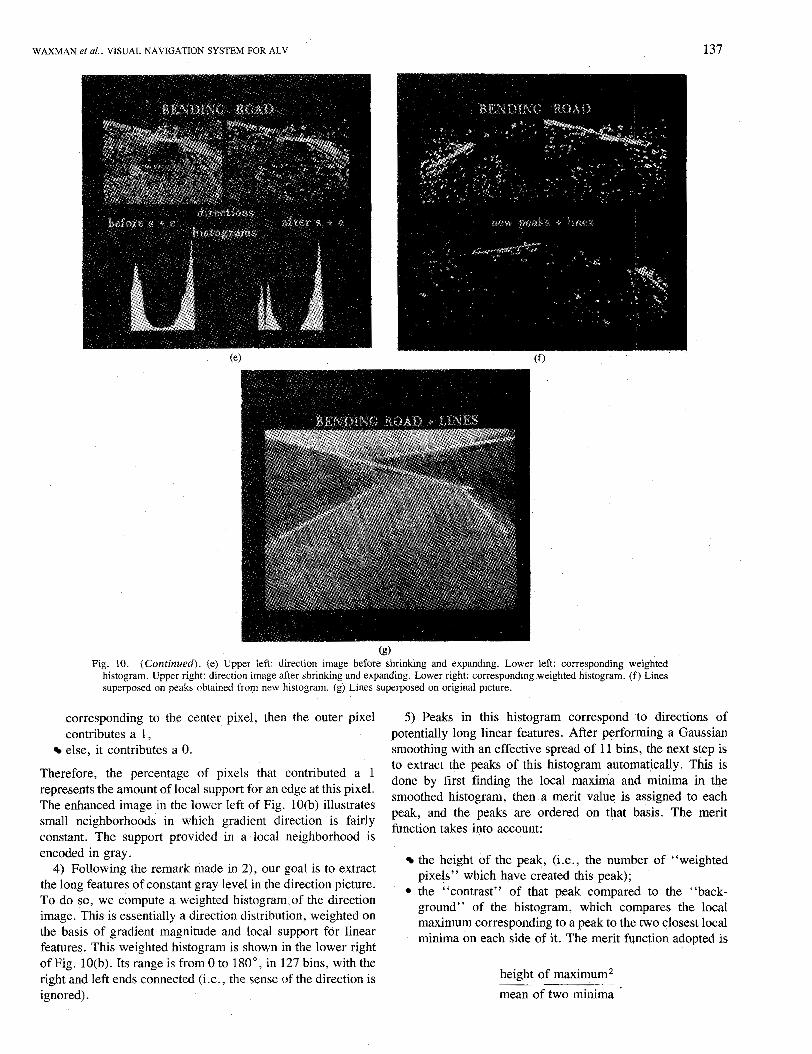
(g) Fig. 10. (Continued). (e) Upper left: direction image before shrinking and expanding. Lower left: corresponding weighted
histogram. Upper right: direction image after shrinking and expanding. Lower right: corresponding weighted histogram. (f) Lines superposed on peaks obtained from new histogram. (g) Lines superposed on original picture.
corresponding to the center pixel, then the outer pixel contributes a I , else, it contributes a 0.
Therefore, the percentage of pixels that contributed a 1 represents the amount of local support for an edge at this pixel. The enhanced image in the lower left of Fig. 10(b) illustrates small neighborhoods in which gradient direction is fairly constant. The support provided in a local neighborhood is encoded in gray. 4) Following the remark made in 2), our goal is to extract
the long features of constant gray level in the direction picture. To do so, we compute a weighted histogram.of the direction image. This is essentially a direction distribution, weighted on the basis of gradient magnitude and local support for linear features. This weighted histogram is shown in the lower right of Fig. 10(b). Its range is from 0 to 180”, in 127 bins, with the right and left ends connected (i.e., the sense of the direction is ignored).
137
5) Peaks in this histogram correspond to directions of potentially long linear features. After performing a Gaussian smoothing with an effective spread of 11 bins, the next step is to extract the peaks of this histogram automatically. This is done by first finding the local maxima and minima in the smoothed histogram, then a merit value is assigned to each peak, and the peaks are ordered on that basis. The merit function takes into account:
the height of the peak, (Le., the number of “weighted pixels” which have created this peak);
4 the “contrast” of that peak compared to the “back- ground” of the histogram, which compares the local maximum corresponding to a peak to the two closest local minima on each side of it. The merit function adopted is
height of maximum2 mean of two minima
138 IEEE JOURNAL OF ROBOTICS AND AUTOMATION, VOL. RA-3, NO. 2 , APRIL 1987
The positions of the pixels in the original image which contribute to each peak are then determined and stored as binary pictures. These peakpictures will have, for the strong peaks, a cluster of points that delineate dominant linear features. The points corresponding to the strongest four peaks are shown in Fig. lO(c).
6 ) The “peak-pictures” created at the previous step are usually prone to a “salt and pepper” kind of noise. Therefore, we try to isolate the clusters by performing a (4-connected) “shrink and expand” procedure on each peak-picture. This shrinks away the isolated points but leaves clusters unaffected. The results of this procedure are shown in Fig. 10(d).
An interesting detail of this processing is the data structure utilized for this shrink and expand procedure. Since the peak picture for each peak is represented by a binary picture, up to eight peaks can be stored in a byte picture (eight bits per pixel). The use of this data structure not only saves memory, but also significantly reduces processing time since the “shrink and expand” operation can now be done in parallel for all peaks.
The shrink operation does not affect image points having a value zero. Using the data structure just mentioned, as the ranges occupied by the peaks are mutually exclusive, at most a single bit any byte can have is a value of one. Therefore, a single pass through the byte picture will suffice to identify all the “ 1 ” pixels whereas eight separate passes, one for each peak, would be needed if each peak picture were stored separately.
An expand procedure, on the other hand, leaves all image points with value one unaffected. The peak-pictures, after having been shrunk and expanded will be combined by a logical OR to form a binary picture which will be used to create a new direction image, as explained later. Therefore, as soon as the expand operation on a pixel representing any one peak results in its value getting changed from zero to one, processing can cease for that pixel.
7) We repeat the histogramming procedure using only points from the &st set of peaks which survived the shrink and expand procedure. A new direction image is created by taking the product of the old direction image with the result of the logical OR after shrink and expand. The upper and lower left quadrants of Fig. 10(e) again show the direction picture and histogram before the shrink and expand procedure. The upper and lower right quadrants show them after this process. Note how much sharper the new direction histogram is.
8) A new set of peaks is now selected from this histogram by the method described previously. The points corresponding to the new strongest four peaks are shown in Fig. 10(f).
9) In each peak-picture, we now try to locate lines of a specified orientation (according to the direction associated with that peak) plus or minus a small amount (according to the width of the peak). We employ a Hough voting procedure. Thus we have .decomposed the two-dimensional Hough prob- lem into two one-dimensional problems: the first one is to find the approximate orientation of the line, then knowing approxi- mately this direction we use a Hough voting procedure to find the intercept of the line. This last step is done by looking for the largest number of points which fall on the line, then the
next largest, and so on until the number of points falls below some percentage of the strongest line. The lines found are shown superposed on the points for each peak in Fig. 10(f).
10) Finally, we locate the clusters of points on the lines found, by histogramming the density of points along and near the lines. Clusters are easily detected since the density histogram typically consists of a few peaks with sharp cutoffs between them. Thus the lines are broken into line segments. Fig. 1O(g) shows all the line segments that are found superposed on the original picture.
This bootstrap processing requires about 90 s CPU time on a VAX 11/785 and is principally spent in the enhancement step and the Hough step; however, the linear enhancement step which requires about a third of this time is often unnecessary. This estimate includes time spent in creating files that will not be needed actually to run the ALV. Besides, during most of the traverse, the ALV will be guided by the feedforward stage, which requires far less processing time.
B. Feedforward Image Processing Once bootstrapping is complete, the locations of dominant
linear features can be predicted near the bottom of the next image. The image processing steps required to extract the dominant linear features in the feedforward mode is a subset of those required in the bootstrapping mode. In particular, no enhancement of linear features is necessary prior to histogram- ming. As we are looking for a feature that is a line segment of width one pixel, inside the area of the image where we are looking, the signal to noise ratio is inversely proportional to the feature length. This implies that for the small windows used in the feedforward mode, linear feature enhancement is unnecessary. Other differences between the two modes also exist in the detection of the peaks after histogramming and in the Hough transform application. The various processing steps applied within a window are as follows.
1) The original picture is artificially blurred to reduce the noise.
2 ) The Sobel operator is then applied to obtain the gradient magnitude and direction.
3) A histogram of the direction is then constructed, weighted on the basis of the square of the gradient magnitude. As previously, this histogram is smoothed by a Gaussian filter and the peaks are automatically selected. Then, if the window under consideration is at the bottom of the picture (i.e., placed by the predictor), the strongest peak is chosen. Otherwise, the single peak chosen is that with direction closest to the line found in the previous window. From this chosen peak, we can then create the corresponding “peak-picture.”
4) We now try to locate a line in the peak picture of a specified orientation plus or minus a small amount. If this is the first window, then the lines are found by the same Hough voting procedure that was described for the bootstrapping mode. Processing differs for subsequent windows because of the introduction of an additional constraint; lines found in these windows must be connected to the ones found in the previous windows. This constraint follows naturally from the constraint in the real world of road continuity. Finding the line in this case becomes much easier because the intercept of
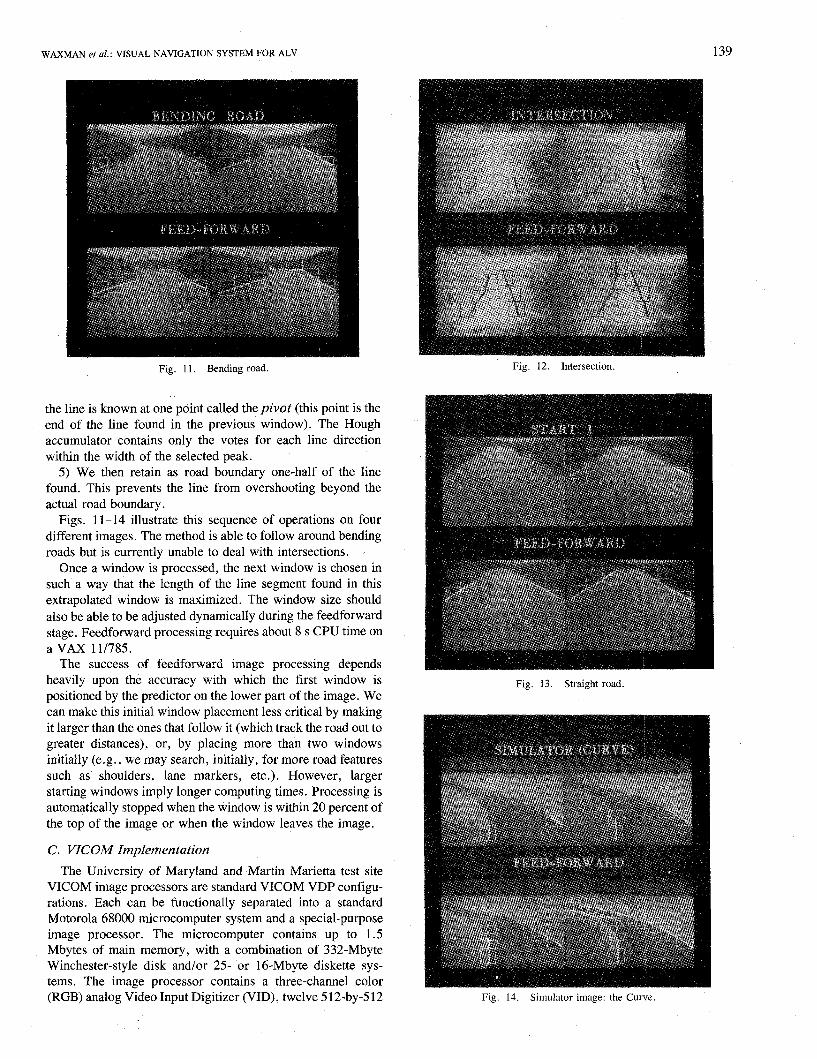
WAXMAN et al.: VISUAL NAVIGATION SYSTEM FOR ALV 139
Fig. 11. Bending road. Fig. 12. Intersection.
the line is known at one point called the pivot (this point is the end of the line found in the previous window). The Hough accumulator contains only the votes for each line direction within the width of the selected peak.
5 ) We then retain as road boundary one-half of the line found. This prevents the line from overshooting beyond the actual road boundary.
Figs. 11-14 illustrate this sequence of operations on four different images. The method is able to follow around bending roads but is currently unable to deal with intersections. '
Once a window is processed, the next window is chosen in such a way that the length of the line segment found in this extrapolated window is maximized. The window size should also be able to be adjusted dynamically during the feedforward stage. Feedforward processing requires about 8 s CPU time on a VAX 11/785.
The success of feedforward image processing depends heavily upon the accuracy with which the first window is positioned by the predictor on the lower part of the image. We can make this initial window placement less critical by making it larger than the ones that follow it (which track the road out to greater distances), or, by placing more than two windows initially (e.g., we may search, initially, for more road features such as shoulders, lane markers, etc.). However, larger starting windows imply longer computing times. Processing is automatically stopped when the window is within 20 percent of the top of the image ,or when the window leaves the image.
C. VICOM Implementation The University of Maryland and Martin Marietta test site
VICOM image processors are standard VICOM VDP configu- rations. Each can be functionally separated into a standard Motorola 68000 microcomputer system and a special-purpose image processor. The microcomputer contains up to 1.5 Mbytes of main memory, with a combination of 332-Mbyte Winchester-style disk andfor 25- or 16-Mbyte diskette sys- tems. The image processor contains a three-channel color
Fig. 13. Straight road
(RGB) analog Video Input Digitizer (VID), twelve 512-by-512 Fig. 14. Simulator image: the Curve.
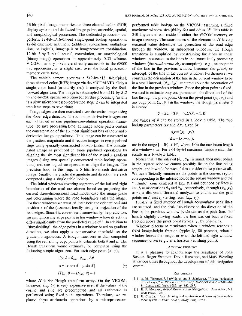
140 IEEE JOURNAL OF ROBOTICS AND AUTOMATION, VOL. RA-3, NO. 2, APRIL 1987
16-bit-pixel image memories, a three-channel color (RGB) display system, and dedicated image point, ensemble, spatial, and morphological processors. The dedicated processors can perform 12-bit-id16-bit-out single-point lookup operations, 12-bit ensemble arithmetic (addition, subtraction, multiplica- tion, or logical), image-pair or image/constant combination, 12-bit 3-by-3 pixel spatial convolution, or morphological (binary-image) operations in approximately 0.33 s/frame. VICOM memory pixels are directly accessible to the 68000 microprocessor, at a slight cost over the local processor- memory cycle time.
The vehicle camera acquires a 512-by-512, 8-bit/pixel, three-channel color (RGB) image via the VICOM VID. Only a single color band (ordinarily red) is analyzed by the feed- forward algorithm. The image is subsampled from 512-by-512 to 256-by-256 spatial resolution for further processing (as this is a slow microprocessor-performed step, it can be integrated into later steps to save time).
Image edges are then extracted over the entire image using the Sobel edge detector. The x- and y-derivative images are each obtained in one pipeline-convolution operation frame- time. To save processing time, an image whose pixels contain the concatenation of the six most significant bits of the x and y derivative image is produced. This image can be converted to the gradient magnitude and direction images in two pipelined steps using specially constructed lookup tables. The concate- nated image is produced in three pipelined operations by aligning the six most significant bits of the x and y gradient images (using two specially constructed table lookup opera- tions) and one logical OR operation to align the images. The precision loss, in this step, is 5 bits from each derivative image. Finally, the gradient magnitude and direction are each computed using a single table lookup.
The initial windows covering segments of the left and right boundaries of the road are chosen based on projecting the current three-dimensional road model onto the image plane and determining where the road boundaries enter the image. For these windows we must estimate both the orientation 8 and position p of the (assumed locally straight) projection of the road edges. Since 0 is constrained somewhat by the prediction, we can ignore any edge points in the window whose directions differ significantly from the predicted value of 8. In addition to “thresholding” the edge points in a window based on gradient direction, we also apply a conservative threshold on the gradient magnitudes. A Hough transform is then computed using the remaining edge points to estimate both 0 and p . The Hough transform would ordinarily be computed using the following simple algorithm. For each edge point (x, y ) ,
for 8 = Omin, Omax, A8
p = [x CQS 8 + y sin 81 (*I H ( P , 0) = ~ ( p , e ) + 1
where H is the Hough transform array. On the VICOM, however, step (*) is very expensive even if the values of the cosine and sine are precomputed and all arithmetic is performed using fixed-point operations. Therefore, we re- placed these arithmetic operations by a microprocessor-
performed table lookup on the VICOM, assuming a fixed maximum window size (64-by-64) and A8 = 3O. This table is 240 kbytes and can reside in either the VICOM memory or image memory. The coordinates of the element in H having maximal value determine the projection of the road edge through the window. In subsequent windows, the Hough transform is simplified by constraining the lines in these windows to connect to the lines in the immediately preceding windows (the road continuity assumption)-e.g., an endpoint of the line in the previous window becomes the pivot, or intercept, of the line in the current window. Furthermore, we constrain the orientation of the line in the current window to be in a small interval, [e,, O M ] , centered about the orientation of the line in the previous window. Since the pivot point is fixed, we need to estimate only one parameter-the direction 6’ of the line through the pivot point. Given the pivot point (xp, yp) and any edge point (x”, y,) in the window, the Hough parameter 8 is simply
8=tan-1((yu-yp)/(x,-xD)).
The values of 8 can be stored in a lookup table. The two lookup parameters Ay and Ax, given by
AY = ( Y , - Y p >
A X = ( X , - X ~ ) , are in the range [ - W, + W ] where Wis the maximum length of a window side. For a 64-by-64 maximum window size, this results in a 16-kbyte table.
Notice that if the interval [e,, O M ] is small, then most points in the square window cannot possibly lie on the line being sought, and it would be wasteful to consider those points at all. We can efficiently enumerate the points in the convex region corresponding to the intersection of the square window and the “infinite” cone centered at (xp, y p ) and bounded by lines 1, and l2 at orientations Om and O M , respectively, through (xp, y p ) using a discrete differential analyzer to enumerate the grid points on 1, and l2 starting from (xp, yp).
Finally, a fixed number of Hough accumulator peak lines are selected, and the peak line closest to the direction of the line in the previous window is chosen as the peak line. To handle slightly curving roads, the line was cut back a fixed fraction above the pivot point (typically, by one-half).
Window placement terminates when a window reaches a fixed image-height fraction (typically, 80 percent), when a window leaves the image, or when the left and right window sequences cross (e.g., at a horizon vanishing point).
ACKNOWLEDGMENT It is a pleasure to acknowledge the assistance of John
Bosque, Roger Eastman, David Harwood, and Mark Westling at various times throughout the development of this navigation system.
REFERENCES
[I] A. M. Waxman, J. LeMoigne, and B. Srinivasan, “Visual navigation of roadways,” in 1985 IEEE Int. Conf. Robotics and Automation, St. Louis, MO, Mar. 1985, pp. 862-867.
[2] H . P. Moravec, Robot Rover Visual Navigation. Ann Arbor, MI: UMI Press, 1981.
[3] R. Chatila, “Path planning and environmental learning in a mobile robot system,” Proc. ECAI, Orsay, Aug. 1982.
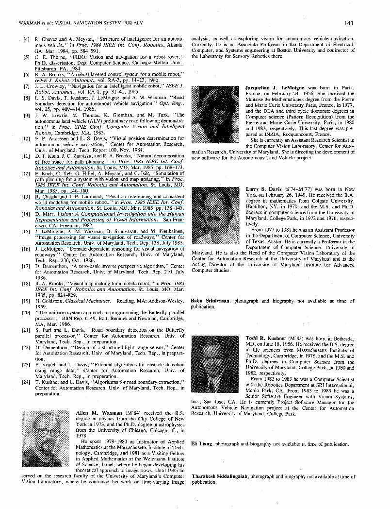
WAXMAN et al. : VISUAL NAVIGATION SYSTEM FOR ALV
R. Chavez and A. Meystel, “Structure of intelligence for an autono- mous vehicle,” in Proc. 1984 IEEE Int. Conf. Robotics, Atlanta, GA, Mar. 1984, pp. 584-591. C. E. Thorpe, “FIDO: Vision and navigation for a robot rover,” Ph.D. dissertation, Dep. Computer Science, Carnegie-Mellon Univ., Pittsburgh, PA, 1984. R. A. Brooks, “A robust layered control system for a mobile robot,” IEEE J. Robot. Automat., vol. RA-2, pp. 14-23, 1986. J. L. Crowley, “Navigation for an intelligent mobile robot,” IEEE J. Robot. Automat., vol. RA-1, pp. 31-41, 1985. L. S. Davis, T. Kushner, J. LeMoigne, and A. M. Waxman, “Road boundary detection for autonomous vehicle navigation,” Opt. Eng.,
J. W. Lowrie, M: Thomas, K. Gremban, and M. Turk, “The autonomous laud vehicle (ALV) preliminary road following demonstra- tion,” in Proc. SPIE Conf. Computer Vision and Intelligent Robots, Cambridge, MA, 1985. F. P. Andresen and L. S. Davis, “Visual position determination for autonomous vehicle navigation,” Center for Automation Research, Univ. of Maryland, Tech. Report 100, Nov.. 1984. D. T. Kuan, J. C. Zamiska, and R. A. Brooks, “Natural decomposition of free space for path planning,” in Proc. 1985 IEEE Int. Conf. Robotics and Automation, St. Louis, MO, Mar. 1985, pp. 168-173. E. Koch, C. Yeh, G. Hillel, A. Meystel, and C. Isik, “Simulation of path planning for a system with vision and map updating,” in Proc. 1985 IEEE Int. Conf. Robotics and Automation, St. Louis, MO, Mar. 1985, pp. 146-160. R. Chatila and J.-P. Laumond, “Position referencing and consistent world modeling for mobile robots,” in Proc. 1985 IEEE Int. Conf. Robotics andAutomation, St. Louis, MO, Mar. 1985, pp. 138-145. D. Marr, Vision: A Computational Investigation into the Human Representation and Processing of Visual Information. San Fran- cisco, CA: Freeman, 1982. J. LeMoigne, A. M. Waxman, B. Srinivasan, and M. Pietikainen, “Image processing for visual navigation of roadways,” Center for Automation Research, Univ. of Maryland, Tech. Rep. 138, July 1985. J. LeMoigne, “Domain-dependent reasoning for visual navigation of roadways,” Center for Automation Research, Univ. of Maryland, Tech. Rep. 230, Oct. 1986. D. Dementhon, “A zero-bank inverse perspective algorithm,” Center for Automation Research, Univ: of Maryland, Tech. Rep. 210, July 1986. R. A. Brooks, “Visual map making for a mobile robot,” in Proc. I985 IEEE Int. Conf. Robotics and Automation, St. Louis, MO, Mar.
H. Goldstein, ClassicalMechanics. Reading, MA: Addison-Wesley, 1959. “The uniform system approach to programming the Butterfly parallel processor,” BBN Rep. 6149, Bolt, Beranek and Newman, Cambridge, MA, Mar. 1986. S. Puri and L. Davis, “Road boundary detection on the Butterfly parallel processor,” Center for Automation Research, Univ. of Maryland, Tech. Rep., in preparation. D. Dementhon, “Design of a structured-light range sensor,” Center for Automation Research, Univ. of Maryland, Tech. Rep., in prepara- tion. P. Veatch and L. Davis, “Efficient algorithms for obstacle detection using range data,” Center for Automation Research, Univ. of Maryland, Tech. Rep., in preparation. T. Kushner and L. Davis, “Algorithms for road boundary extraction,” Center for Automation Research, Univ. of Maryland, Tech. Rep., in preparation.
V O ~ . 25, pp. 409-414, 1986.
1985, pp. 824-829.
141
analysis, as well as exploring vision for autonomous vehicle navigation. Currently, he is an Associate Professor in the Department of Electrical, Computer, and Systems engineering at Boston University and codirector of the Laboratory for Sensory Robotics there.
Jacqueline J. LeMoigne was born in Paris, France, on February 24, 1956. She received the Maitrise de Mathematiques degree from the Pierre and Marie Curie University Paris, France, in 1977, and the DEA and third cycle doctorate degrees in Computer science (Pattern Recognition) from the Pierre and Marie Curie University, Paris, in 1980 and 1983, respectively. This last degree was pre- pared at INRIA, Rocquencourt, France.
She is currently an Assistant Research Scientist in the Computer Vision Laboratory, Center for Auto-
mation Research, University of Maryland. She is directing the development of new software for the Autonomous Land Vehicle project.
Larry S. Davis (S’74-M’77) was born in New York on February 26, 1949. He received the B.A. degree in mathematics from Colgate University, Hamilton, NY, in 1970, and the M.S. and Ph.D. degrees in computer science from the University of Maryland, College Park, in 1972 and 1976, respec- tively.
From 1977 to 1981 he was an Assistant Professor in the Department of Computer Science, University of Texas, Austin. He is currently a Professor in the Department of Computer Science, University of
Maryland. He is also the Head of the Computer Vision Laboratory of the Center for Automation Research at the University of Maryland and is the Acting Director of the University of Maryland Institute for Advanced Computer Studies.
Babu Srinivasan, photograph and biography not available at time of publication.
Todd R. Kushner (”83) was born in Bethesda, MD, on June 18, 1956. He received the B.S. degree in life sciences from Massachusetts Institute of Technology, Cambridge, in 1976, and the M.S. and Ph.D. degrees in Computer Science from the University of Maryland, College Park, in 1980 and 1982, respectively.
From 1982 to 1983 he was a Computer Scientist with the Robotics Department at SRI International, Menlo Park, CA. From 1983 to 1985 he was a Senior Software Engineer with Vicom Systems,
Inc., San Jose, CA. He is currently Project Software Manager for the Autonomous Vehicle Navigation project at the Center for Automation Research, University of Maryland, College Park.
Eli Liang, photograph and biography not available at time of publication.
Tharakesh Siddalingaiah, photograph and biography not available at time of publication.