Integrated GPS/INS Navigation System Design for Autonomous Spacecraft Rendezvous

Copyright

by

David Edward Gaylor

2003

The Dissertation Committee for David Edward Gaylorcertifies that this is the approved version of the following dissertation:

Integrated GPS/INS Navigation System Design for

Autonomous Spacecraft Rendezvous

Committee:

E. Glenn Lightsey, Supervisor

Robert H. Bishop

Wallace T. Fowler

Bob E. Schutz

Kevin W. Key



by

David Edward Gaylor, B.S., M.S.

DISSERTATION

Presented to the Faculty of the Graduate School of

The University of Texas at Austin

in Partial Fulfillment

of the Requirements

for the Degree of

DOCTOR OF PHILOSOPHY

THE UNIVERSITY OF TEXAS AT AUSTIN

December 2003

Acknowledgments

I would like to thank my advisor, Dr. Glenn Lightsey, for his enthusias-

tic support and guidance throughout this research. I would also like to thank

my committee members: Dr. Robert Bishop, Dr. Wallace Fowler, and Dr.

Bob Schutz of the Aerospace Engineering Department, and Dr. Kevin Key of

Titan Corporation at the NASA Johnson Space Center, for their assistance in

the preparation of this manuscript.

This research was partially funded by the NSTL Relative Navigation

Support Grant (NAG9-1189) from the Navigation Systems and Technology

Laboratory at the NASA Johnson Space Center. I would like to thank Janet

Bell and Susan Gomez for supporting this research and Daniel Adamo, John

Goodman, and Tim Crain for their technical support.

This is the third in a series of dissertations on the topic of GPS navi-

gation for spacecraft rendezvous applications, so I would like to acknowledge

the work of Takuji Ebinuma and Jaeyong Um, which provided the foundation

for this research. I would also like to thank Oliver Montenbruck for allowing

me to translate his SAT_Lib software library to Java.

The results presented in this dissertation were produced using software

from the Java Astrodynamics Toolkit, an open source software library, which

can be found on the Internet at: http://jat.sourceforge.net.

iv



Publication No.

David Edward Gaylor, Ph.D.

The University of Texas at Austin, 2003

Supervisor: E. Glenn Lightsey

The goal of the NASA Space Launch Initiative (SLI) program is to

advance the technologies for the next generation reusable launch vehicle (RLV).

The SLI program has identified automated rendezvous and docking as an area

requiring further research and development. Currently, the Space Shuttle uses

a partially manual system for rendezvous, but a fully automated system could

be safer and more reliable.

Previous studies have shown that it is feasible to use the Global Po-

sitioning System (GPS) for spacecraft navigation during rendezvous with the

International Space Station (ISS). However, these studies have not accounted

for the effects of GPS signal blockage and multipath in the vicinity of the ISS,

which make a GPS-only navigation system less accurate and reliable.

One possible solution is to combine GPS with an inertial navigation

system (INS). The integration of GPS and INS can be achieved using a Kalman

v

filter. GPS/INS systems have been used in aircraft for many years and have

also been used in launch vehicles. However, the performance of GPS/INS

systems in orbit and during spacecraft rendezvous has not been characterized.

The primary objective of this research is to evaluate the ability of an

integrated GPS/INS to provide accurate navigation solutions during a ren-

dezvous scenario where the effects of ISS signal blockage, multipath and delta-v

maneuvers degrade GPS-only navigation. In order to accomplish this, GPS-

only and GPS/INS Kalman filters have been developed for both absolute and

relative navigation, as well as a new statistical multipath model for spacecraft

operating near the ISS.

Several factors that affect relative navigation performance were stud-

ied, including: filter tuning, GPS constellation geometry, rendezvous approach

direction, and inertial sensor performance. The results showed that each of

these factors has a large impact on relative navigation performance.

Finally, it has been demonstrated that a GPS/INS system based on

medium accuracy aircraft avionics-grade inertial sensors does not provide ad-

equate relative navigation performance for rendezvous with the ISS unless

accelerometer thresholding is used. However, the use of state-of-the-art iner-

tial navigation sensors provides relative position accuracy which is adequate

for rendezvous with ISS if an additional rendezvous sensor is included.

vi

Table of Contents

Acknowledgments iv

Abstract v

List of Tables xiii

List of Figures xv

Chapter 1. Introduction 1

1.1 Background . . . . . . . . . . . . . . . . . . . . . . . . . . . . 1

1.2 Previous Work . . . . . . . . . . . . . . . . . . . . . . . . . . . 5

1.3 Research Contributions . . . . . . . . . . . . . . . . . . . . . . 7

1.3.1 INS Error Model . . . . . . . . . . . . . . . . . . . . . . 7

1.3.2 ISS Signal Blockage Model . . . . . . . . . . . . . . . . 7

1.3.3 ISS Multipath Model . . . . . . . . . . . . . . . . . . . 8

1.3.4 GPS/INS Extended Kalman Filter Design and Analysis 8

1.3.5 Rendezvous Simulation and Navigation Design Tool . . 10

1.4 Overview . . . . . . . . . . . . . . . . . . . . . . . . . . . . . . 11

Chapter 2. Coordinate and Time Systems 12

2.1 Reference Frames . . . . . . . . . . . . . . . . . . . . . . . . . 12

2.1.1 Earth Centered Inertial (ECI) . . . . . . . . . . . . . . . 13

2.1.2 Earth Centered Earth Fixed (ECEF) . . . . . . . . . . . 13

2.1.3 Spacecraft Centered (UVW) . . . . . . . . . . . . . . . 13

2.1.4 Body Frame . . . . . . . . . . . . . . . . . . . . . . . . 14

2.1.5 Navigation Frame . . . . . . . . . . . . . . . . . . . . . 15

2.1.6 Coordinate Transformations . . . . . . . . . . . . . . . . 15

2.1.7 Quaternions . . . . . . . . . . . . . . . . . . . . . . . . 16

2.1.8 Small Angle Transformations . . . . . . . . . . . . . . . 18

vii

2.2 Time Systems . . . . . . . . . . . . . . . . . . . . . . . . . . . 18

2.2.1 Time Scales . . . . . . . . . . . . . . . . . . . . . . . . . 19

2.2.2 Time Formats . . . . . . . . . . . . . . . . . . . . . . . 20

Chapter 3. GPS Measurement Models 21

3.1 GPS Constellation Model . . . . . . . . . . . . . . . . . . . . . 22

3.1.1 GPS Ephemeris Parameters . . . . . . . . . . . . . . . . 22

3.1.2 GPS SV Position Equations . . . . . . . . . . . . . . . . 23

3.1.3 GPS SV Velocity Equations . . . . . . . . . . . . . . . . 26

3.2 GPS Measurement Equations . . . . . . . . . . . . . . . . . . . 27

3.2.1 Pseudorange Measurement . . . . . . . . . . . . . . . . 27

3.2.2 Range Rate Equation . . . . . . . . . . . . . . . . . . . 29

3.2.3 Carrier Phase Measurement . . . . . . . . . . . . . . . . 29

3.2.4 Satellite Motion During Signal Propagation . . . . . . . 30

3.3 GPS Measurement Error Models . . . . . . . . . . . . . . . . . 31

3.3.1 Pseudorange and Carrier Phase . . . . . . . . . . . . . . 31

3.3.2 Single Difference Carrier Phase . . . . . . . . . . . . . . 32

3.4 ISS Blockage and Multipath Models . . . . . . . . . . . . . . . 33

3.4.1 ISS Signal Blockage Model . . . . . . . . . . . . . . . . 33

3.4.2 ISS Multipath Model . . . . . . . . . . . . . . . . . . . 36

3.4.3 GPS Carrier Phase Measurement Errors . . . . . . . . . 39

3.4.4 GPS C/A Code Measurement Errors . . . . . . . . . . . 39

3.4.4.1 Conjectures . . . . . . . . . . . . . . . . . . . . 41

3.4.4.2 Multipath Model Algorithm . . . . . . . . . . . 45

3.5 ISS and Spacecraft Orbit Models . . . . . . . . . . . . . . . . . 46

3.6 ISS Blockage Study Results . . . . . . . . . . . . . . . . . . . . 46

3.7 Multipath Study Results . . . . . . . . . . . . . . . . . . . . . 48

3.7.1 Geometry Dependence . . . . . . . . . . . . . . . . . . . 48

3.7.2 Distance from ISS . . . . . . . . . . . . . . . . . . . . . 49

3.7.3 Number of Multipath Rays . . . . . . . . . . . . . . . . 50

3.7.4 ISS Radar Cross-sectional Area . . . . . . . . . . . . . . 51

3.7.5 Model Tuning and Validation . . . . . . . . . . . . . . . 54

viii

Chapter 4. Inertial Navigation 56

4.1 Fundamentals of Inertial Navigation . . . . . . . . . . . . . . . 56

4.2 INS Error Sources . . . . . . . . . . . . . . . . . . . . . . . . . 58

4.2.1 Initialization Errors . . . . . . . . . . . . . . . . . . . . 58

4.2.2 System Alignment Errors . . . . . . . . . . . . . . . . . 58

4.2.3 Sensor Errors . . . . . . . . . . . . . . . . . . . . . . . . 58

4.2.3.1 Gyro Measurement Noise . . . . . . . . . . . . 59

4.2.3.2 Gyro Drift (Bias) . . . . . . . . . . . . . . . . 59

4.2.3.3 Gyro Scale Factor . . . . . . . . . . . . . . . . . 59

4.2.3.4 Gyro Misalignments . . . . . . . . . . . . . . . 60

4.2.3.5 Gyro G-Sensitivity . . . . . . . . . . . . . . . . 60

4.2.3.6 Accelerometer Measurement Noise . . . . . . . 60

4.2.3.7 Accelerometer Bias . . . . . . . . . . . . . . . 60

4.2.3.8 Accelerometer Scale Factor . . . . . . . . . . . . 61

4.2.3.9 Accelerometer Misalignments . . . . . . . . . . 61

4.2.3.10 Accelerometer Non-linearity . . . . . . . . . . . 61

4.2.4 Gravity Model Errors . . . . . . . . . . . . . . . . . . . 61

4.2.5 Quantization and Computational Errors . . . . . . . . . 61

4.3 INS Error Model . . . . . . . . . . . . . . . . . . . . . . . . . 62

4.3.1 Derivation of INS Error Model . . . . . . . . . . . . . . 62

4.3.2 Sensor Error Models . . . . . . . . . . . . . . . . . . . . 65

4.3.2.1 Gyro Error Model . . . . . . . . . . . . . . . . 65

4.3.2.2 Accelerometer Error Model . . . . . . . . . . . 66

4.3.3 Augmented INS Error Model . . . . . . . . . . . . . . . 67

4.3.3.1 Adding Gyro and Accelerometer Bias States . . 68

Chapter 5. GPS/INS Integration and Simulation 70

5.1 GPS/INS Simulation Description . . . . . . . . . . . . . . . . 70

5.1.1 Rendezvous Trajectory Generation . . . . . . . . . . . . 70

5.1.1.1 Rendezvous Guidance . . . . . . . . . . . . . . 73

5.1.1.2 Intercept Equation . . . . . . . . . . . . . . . . 73

5.1.1.3 Glideslope Targeting . . . . . . . . . . . . . . . 74

ix

5.1.1.4 Converting Impulses to Finite Burns . . . . . . 76

5.1.1.5 Open Loop vs. Closed Loop Guidance . . . . . 77

5.1.1.6 R-bar Approach . . . . . . . . . . . . . . . . . . 78

5.1.1.7 V-bar Approach . . . . . . . . . . . . . . . . . . 81

5.1.2 Generation of Simulated INS Measurements . . . . . . . 84

5.1.3 GPS Measurement Generation . . . . . . . . . . . . . . 89

5.1.3.1 Pseudorange and Carrier Phase Measurements . 89

5.1.3.2 Single Difference Carrier Phase Measurements . 90

5.1.3.3 GPS Receiver Clock Model . . . . . . . . . . . 91

5.1.3.4 Ionospheric Delay . . . . . . . . . . . . . . . . . 92

5.1.3.5 SV Clock and Ephemeris Errors . . . . . . . . . 94

5.1.3.6 Integer Ambiguity . . . . . . . . . . . . . . . . 95

5.2 GPS/INS Integration . . . . . . . . . . . . . . . . . . . . . . . 95

5.2.1 Extended Kalman Filter Equations . . . . . . . . . . . . 97

5.2.2 Numerical Integration of INS Solution . . . . . . . . . . 98

5.2.2.1 Analysis of Integration Algorithm Accuracy . . 100

5.2.3 State Propagation Models . . . . . . . . . . . . . . . . . 101

5.2.3.1 Earth Gravity Model . . . . . . . . . . . . . . . 102

5.2.3.2 Atmospheric Drag Model . . . . . . . . . . . . . 102

5.2.3.3 Drag Coefficient Correction State . . . . . . . . 103

5.2.3.4 Gyro and Accelerometer Bias States . . . . . . 104

5.2.3.5 GPS Receiver Clock States . . . . . . . . . . . . 104

5.2.3.6 Ionospheric Delay State . . . . . . . . . . . . . 104

5.2.3.7 URE State . . . . . . . . . . . . . . . . . . . . . 105

5.2.3.8 Integer Ambiguity State . . . . . . . . . . . . . 105

5.2.4 Process Noise Covariance . . . . . . . . . . . . . . . . . 106

5.2.5 Measurement Models . . . . . . . . . . . . . . . . . . . 107

5.2.5.1 Measurement Noise Covariance . . . . . . . . . 108

5.2.6 GPS/INS Absolute Navigation Filter . . . . . . . . . . . 109

5.2.7 GPS/INS Relative Navigation Filter . . . . . . . . . . . 110

5.2.8 GPS-only Relative Navigation Filter . . . . . . . . . . . 111

x

Chapter 6. GPS/INS Simulation Results 112

6.1 Absolute Navigation . . . . . . . . . . . . . . . . . . . . . . . . 112

6.1.1 C/A Code vs. Carrier Phase Measurements . . . . . . . 112

6.1.2 Absolute Navigation Filter Results . . . . . . . . . . . . 115

6.2 Relative Navigation . . . . . . . . . . . . . . . . . . . . . . . . 125

6.2.1 State Vector vs. Measurement Differencing . . . . . . . 126

6.2.2 Addition of a Thrust Model in GPS-Only Filter . . . . . 129

6.2.3 Filter Tuning . . . . . . . . . . . . . . . . . . . . . . . . 132

6.2.3.1 GPS-Only Filter Tuning . . . . . . . . . . . . . 132

6.2.3.2 GPS/INS Filter Tuning . . . . . . . . . . . . . 142

6.2.3.3 Tuning Comparison . . . . . . . . . . . . . . . . 155

6.2.4 Constellation Geometry and Approach Directions . . . . 159

6.2.5 Accelerometer Thresholding . . . . . . . . . . . . . . . . 162

6.2.6 Improved Inertial Sensors . . . . . . . . . . . . . . . . . 163

6.2.7 Use of GPS Satellites Below the Horizon . . . . . . . . . 167

6.2.8 Gain Scheduling . . . . . . . . . . . . . . . . . . . . . . 169

6.2.9 Monte Carlo Study . . . . . . . . . . . . . . . . . . . . . 170

Chapter 7. Conclusions 175

7.1 Summary of Results . . . . . . . . . . . . . . . . . . . . . . . . 175

7.2 Future Work . . . . . . . . . . . . . . . . . . . . . . . . . . . . 181

Appendices 185

Appendix A. Unaided INS Simulation Results 186

A.1 Unforced Error Response . . . . . . . . . . . . . . . . . . . . . 187

A.1.1 Response to Initial Position Errors . . . . . . . . . . . . 188

A.1.2 Response to Initial Velocity Errors . . . . . . . . . . . . 190

A.1.3 Response to Initial Platform Tilts . . . . . . . . . . . . 192

A.2 Forced Error Response . . . . . . . . . . . . . . . . . . . . . . 194

A.2.1 Zero Specific Force Case . . . . . . . . . . . . . . . . . . 194

A.2.1.1 Response to Gyro Scale Factor Error and Mis-alignments . . . . . . . . . . . . . . . . . . . . . 194

xi

A.2.1.2 Response to Constant Gyro Biases . . . . . . . 196

A.2.1.3 Response to Gyro Measurement Noise . . . . . 197

A.2.2 Constant Specific Force Cases . . . . . . . . . . . . . . . 198

A.2.2.1 Response to Gyro Errors . . . . . . . . . . . . . 198

A.2.2.2 Response to Accelerometer Scale Factor Error . 205

A.2.2.3 Response to Accelerometer Misalignments . . . 208

A.2.2.4 Response to Constant Accelerometer Biases . . 212

A.2.2.5 Response to Accelerometer Measurement Noise 214

A.3 Conclusions . . . . . . . . . . . . . . . . . . . . . . . . . . . . 217

Appendix B. Stochastic Process Models 219

B.1 White Gaussian Noise . . . . . . . . . . . . . . . . . . . . . . . 219

B.2 Gaussian Random Constant . . . . . . . . . . . . . . . . . . . 219

B.3 Random Walk . . . . . . . . . . . . . . . . . . . . . . . . . . . 220

B.4 First Order Markov . . . . . . . . . . . . . . . . . . . . . . . . 220

B.5 Equivalent Discrete-Time Models . . . . . . . . . . . . . . . . 220

B.5.1 First Order Markov . . . . . . . . . . . . . . . . . . . . 222

B.5.2 Random Walk . . . . . . . . . . . . . . . . . . . . . . . 222

Bibliography 223

Vita 230

xii

List of Tables

1.1 Space Shuttle Navigation Sensors[18] . . . . . . . . . . . . . . 2

3.1 GPS Satellite Ephemeris Parameters [33] . . . . . . . . . . . . 23

3.2 ISS Orbit Elements. . . . . . . . . . . . . . . . . . . . . . . . . 46

3.3 GPS Signal Outage Statistics (All-In-View Receiver) . . . . . 47

5.1 Spacecraft Characteristics . . . . . . . . . . . . . . . . . . . . 72

5.2 Chaser Nominal Thrust for Each Maneuver Type . . . . . . . 76

5.3 Initial ISS Orbit Elements . . . . . . . . . . . . . . . . . . . . 78

5.4 R-bar Approach Guidance Targets . . . . . . . . . . . . . . . . 79

5.5 R-bar Approach Maneuvers . . . . . . . . . . . . . . . . . . . 79

5.6 V-bar Approach Guidance Targets . . . . . . . . . . . . . . . 82

5.7 V-bar Approach Maneuvers . . . . . . . . . . . . . . . . . . . 82

5.8 SIGI Sensor Characteristics [41] . . . . . . . . . . . . . . . . . 88

5.9 Observed Ephemeris and Clock Errors . . . . . . . . . . . . . 94

5.10 Exponential Atmospheric Model [42] . . . . . . . . . . . . . . 103

5.11 GPS/INS Absolute Navigation Filter States . . . . . . . . . . 109

5.12 GPS/INS Relative Navigation Filter States . . . . . . . . . . . 110

5.13 GPS-only Relative Navigation Filter States . . . . . . . . . . . 111

6.1 Multipath Model Parameters . . . . . . . . . . . . . . . . . . . 115

6.2 GPS/INS Absolute Navigation Filter Process Noise . . . . . . 117

6.3 GPS-Only Absolute Navigation Filter Process Noise . . . . . . 117

6.4 GPS/INS vs GPS-Only Absolute Navigation Comparison . . . 124

6.5 GPS-Only Relative Navigation Filter Process Noise . . . . . . 133

6.6 GPS/INS Relative Navigation Filter Process Noise . . . . . . 143

6.7 Relative Navigation Filter Tuning Comparison . . . . . . . . . 156

6.8 GPS-only Relative Navigation Performance . . . . . . . . . . . 161

xiii

6.9 GPS/INS Relative Navigation Performance . . . . . . . . . . . 162

6.10 GPS/INS Relative Navigation Performance, Accelerometer Thresh-olding . . . . . . . . . . . . . . . . . . . . . . . . . . . . . . . 163

6.11 SIMU Sensor Characteristics . . . . . . . . . . . . . . . . . . . 165

6.12 GPS/SIMU Relative Navigation Performance . . . . . . . . . 166

6.13 GPS-only Relative Navigation Performance, Relative Naviga-tion Tuning . . . . . . . . . . . . . . . . . . . . . . . . . . . . 168

6.14 GPS/SIMU Relative Navigation Performance, Relative Naviga-tion Tuning . . . . . . . . . . . . . . . . . . . . . . . . . . . . 168

6.15 Relative Navigation Gain Scheduling vs. Relative NavigationTuning Comparison . . . . . . . . . . . . . . . . . . . . . . . . 170

6.16 Monte Carlo Study Results . . . . . . . . . . . . . . . . . . . . 172

A.1 Simulation Orbit Parameters . . . . . . . . . . . . . . . . . . . 186

xiv

List of Figures

3.1 The ISS Blockage and Multipath Scenario . . . . . . . . . . . 33

3.2 Line of Sight Vector Definitions . . . . . . . . . . . . . . . . . 34

3.3 GPS Signal Blockage Model . . . . . . . . . . . . . . . . . . . 36

3.4 Range Errors and Direct Signal Elevation Angles . . . . . . . 49

3.5 Carrier Phase Range Errors at 50m, 100 m and 200 m Belowthe ISS . . . . . . . . . . . . . . . . . . . . . . . . . . . . . . . 50

3.6 C/A Code Range Errors at 50m, 100 m and 200 m Below the ISS 51

3.7 Carrier Phase Range Errors with Various Numbers of MultipathRays . . . . . . . . . . . . . . . . . . . . . . . . . . . . . . . . 52

3.8 C/A Code Range Errors with Various Numbers of MultipathRays . . . . . . . . . . . . . . . . . . . . . . . . . . . . . . . . 52

3.9 Carrier Phase Range Errors with Different ISS Radar Cross-sectional Areas . . . . . . . . . . . . . . . . . . . . . . . . . . 53

3.10 C/A Code Range Errors with Different ISS Radar Cross-sectionalAreas . . . . . . . . . . . . . . . . . . . . . . . . . . . . . . . . 53

3.11 Blockage and Multipath Simulation Flow Chart . . . . . . . . 55

5.1 R-bar Approach Trajectory . . . . . . . . . . . . . . . . . . . 80

5.2 R-bar Final Approach Trajectory . . . . . . . . . . . . . . . . 80

5.3 R-bar Glideslope Trajectory . . . . . . . . . . . . . . . . . . . 81

5.4 V-bar Approach Trajectory . . . . . . . . . . . . . . . . . . . 83

5.5 V-bar Final Approach Trajectory . . . . . . . . . . . . . . . . 83

5.6 GPS/INS Integration Architecture . . . . . . . . . . . . . . . 96

6.1 Rendezvous Trajectory . . . . . . . . . . . . . . . . . . . . . . 113

6.2 Comparision of Absolute Position Errors Using C/A Code andCarrier Phase Measurements . . . . . . . . . . . . . . . . . . . 114

6.3 Comparision of Absolute Velocity Errors Using C/A Code andCarrier Phase Measurements . . . . . . . . . . . . . . . . . . . 115

6.4 Number of Visible GPS SVs . . . . . . . . . . . . . . . . . . . 116

xv

6.5 Chaser Absolute Navigation Errors, GPS/INS . . . . . . . . . 118

6.6 Quaternion Estimation Errors, GPS/INS . . . . . . . . . . . . 118

6.7 Gyro Bias Estimation Errors, GPS/INS . . . . . . . . . . . . . 119

6.8 Accelerometer Bias Estimation Errors, GPS/INS . . . . . . . . 119

6.9 GPS Receiver Clock Estimation Errors, GPS/INS . . . . . . . 120

6.10 Ionospheric Delay Estimation Errors, GPS/INS . . . . . . . . 120

6.11 GPS SV Clock and Ephemeris Estimation Errors, GPS/INS . 121

6.12 Measurement Residuals, GPS/INS . . . . . . . . . . . . . . . . 121

6.13 Chaser Absolute Navigation Errors, GPS-Only . . . . . . . . . 122

6.14 GPS Receiver Clock Estimation Errors, GPS-Only . . . . . . . 122

6.15 Ionospheric Delay Estimation Errors, GPS-Only . . . . . . . . 123

6.16 GPS SV Clock and Ephemeris Estimation Errors, GPS-Only . 123

6.17 Measurement Residuals, GPS-Only . . . . . . . . . . . . . . . 124

6.18 Relative Position Errors Exchanging Absolute State Vectors . 127

6.19 Relative Velocity Errors Exchanging Absolute State Vectors . 127

6.20 Relative Position Errors Exchanging Measurements . . . . . . 128

6.21 Relative Velocity Errors Exchanging Measurements . . . . . . 128

6.22 GPS-only Relative Position Errors With and Without ThrusterModel . . . . . . . . . . . . . . . . . . . . . . . . . . . . . . . 131

6.23 GPS-only Relative Position Errors With and Without ThrusterModel . . . . . . . . . . . . . . . . . . . . . . . . . . . . . . . 131

6.24 Relative Position Errors, GPS-Only, Nominal Tuning . . . . . 133

6.25 Relative Velocity Errors, GPS-Only, Nominal Tuning . . . . . 134

6.26 Chaser Absolute Navigation Errors, GPS-Only, Nominal Tuning 134

6.27 ISS Absolute Navigation Errors, GPS-Only, Nominal Tuning . 135

6.28 GPS Receiver Clock Estimation Errors, GPS-Only, NominalTuning . . . . . . . . . . . . . . . . . . . . . . . . . . . . . . . 135

6.29 Ionospheric Delay Estimation Errors, GPS-Only, Nominal Tuning136

6.30 GPS SV Clock and Ephemeris Estimation Errors, GPS-Only,Nominal Tuning . . . . . . . . . . . . . . . . . . . . . . . . . . 136

6.31 Integer Ambiguity Estimation Errors, GPS-Only, Nominal Tuning137

6.32 Measurement Residuals, GPS-Only, Nominal Tuning . . . . . 137

6.33 Relative Position Errors, GPS-Only, Relative Navigation Tuning 138

xvi

6.34 Relative Velocity Errors, GPS-Only, Relative Navigation Tuning 138

6.35 Chaser Absolute Navigation Errors, GPS-Only, Relative Navi-gation Tuning . . . . . . . . . . . . . . . . . . . . . . . . . . . 139

6.36 ISS Absolute Navigation Errors, GPS-Only, Relative Naviga-tion Tuning . . . . . . . . . . . . . . . . . . . . . . . . . . . . 139

6.37 GPS Receiver Clock Estimation Errors, GPS-Only, RelativeNavigation Tuning . . . . . . . . . . . . . . . . . . . . . . . . 140

6.38 Ionospheric Delay Estimation Errors, GPS-Only, Relative Nav-igation Tuning . . . . . . . . . . . . . . . . . . . . . . . . . . . 140

6.39 GPS SV Clock and Ephemeris Estimation Errors, GPS-Only,Relative Navigation Tuning . . . . . . . . . . . . . . . . . . . 141

6.40 Integer Ambiguity Estimation Errors, GPS-Only, Relative Nav-igation Tuning . . . . . . . . . . . . . . . . . . . . . . . . . . . 141

6.41 Measurement Residuals, GPS-Only, Relative Navigation Tuning 142

6.42 Relative Position Errors, GPS/INS, Nominal Tuning . . . . . 143

6.43 Relative Velocity Errors, GPS/INS, Nominal Tuning . . . . . 144

6.44 Chaser Absolute Navigation Errors, GPS/INS, Nominal Tuning 144

6.45 ISS Absolute Navigation Errors, GPS/INS, Nominal Tuning . 145

6.46 Quaternion Estimation Errors, GPS/INS, Nominal Tuning . . 145

6.47 Gyro Bias Estimation Errors, GPS/INS, Nominal Tuning . . . 146

6.48 Accelerometer Bias Estimation Errors, GPS/INS, Nominal Tun-ing . . . . . . . . . . . . . . . . . . . . . . . . . . . . . . . . . 146

6.49 GPS Receiver Clock Estimation Errors, GPS/INS, Nominal Tun-ing . . . . . . . . . . . . . . . . . . . . . . . . . . . . . . . . . 147

6.50 Ionospheric Delay Estimation Errors, GPS/INS, Nominal Tuning147

6.51 GPS SV Clock and Ephemeris Estimation Errors, GPS/INS,Nominal Tuning . . . . . . . . . . . . . . . . . . . . . . . . . . 148

6.52 Integer Ambiguity Estimation Errors, GPS/INS, Nominal Tuning148

6.53 Measurement Residuals, GPS/INS, Nominal Tuning . . . . . . 149

6.54 Relative Position Errors, GPS/INS, Relative Navigation Tuning 149

6.55 Relative Velocity Errors, GPS/INS, Relative Navigation Tuning 150

6.56 Chaser Absolute Navigation Errors, GPS/INS, Relative Navi-gation Tuning . . . . . . . . . . . . . . . . . . . . . . . . . . . 150

6.57 ISS Absolute Navigation Errors, GPS/INS, Relative NavigationTuning . . . . . . . . . . . . . . . . . . . . . . . . . . . . . . . 151

xvii

6.58 Quaternion Estimation Errors, GPS/INS, Relative NavigationTuning . . . . . . . . . . . . . . . . . . . . . . . . . . . . . . . 151

6.59 Gyro Bias Estimation Errors, GPS/INS, Relative NavigationTuning . . . . . . . . . . . . . . . . . . . . . . . . . . . . . . . 152

6.60 Accelerometer Bias Estimation Errors, GPS/INS, Relative Nav-igation Tuning . . . . . . . . . . . . . . . . . . . . . . . . . . . 152

6.61 GPS Receiver Clock Estimation Errors, GPS/INS, Relative Nav-igation Tuning . . . . . . . . . . . . . . . . . . . . . . . . . . . 153

6.62 Ionospheric Delay Estimation Errors, GPS/INS, Relative Nav-igation Tuning . . . . . . . . . . . . . . . . . . . . . . . . . . . 153

6.63 GPS SV Clock and Ephemeris Estimation Errors, GPS/INS,Relative Navigation Tuning . . . . . . . . . . . . . . . . . . . 154

6.64 Integer Ambiguity Estimation Errors, GPS/INS, Relative Nav-igation Tuning . . . . . . . . . . . . . . . . . . . . . . . . . . . 154

6.65 Measurement Residuals, GPS/INS, Relative Navigation Tuning 155

6.66 Relative Position Error Comparison . . . . . . . . . . . . . . . 156

6.67 Relative Velocity Error Comparison . . . . . . . . . . . . . . . 157

6.68 Number of Visible GPS SVs vs. Time for Various ConstellationGeometry and Approach Directions . . . . . . . . . . . . . . . 160

6.69 GPS/SIMU Relative Position Error Sigmas During Final Ap-proach . . . . . . . . . . . . . . . . . . . . . . . . . . . . . . . 172

6.70 GPS/SIMU Relative Velocity Error Sigmas During Final Ap-proach . . . . . . . . . . . . . . . . . . . . . . . . . . . . . . . 173

6.71 GPS/SIMU Relative Position Error Sigmas During Filter Con-vergence . . . . . . . . . . . . . . . . . . . . . . . . . . . . . . 173

6.72 GPS/SIMU Relative Velocity Error Sigmas During Filter Con-vergence . . . . . . . . . . . . . . . . . . . . . . . . . . . . . . 174

A.1 Navigation Errors Due to an Initial Radial Position Error . . . 189

A.2 Navigation Errors Due to an Initial Along-track Position Error 189

A.3 Navigation Errors Due to an Initial Cross-track Position Error 190

A.4 Navigation Errors Due to an Initial Radial Velocity Error . . . 191

A.5 Navigation Errors Due to an Initial Along-track Velocity Error 192

A.6 Navigation Errors Due to an Initial Cross-track Velocity Error 193

A.7 Tilt Errors Due to Initial Tilt Errors . . . . . . . . . . . . . . 193

A.8 Tilt Errors Due to Gyro Scale Factor and Misalignments . . . 195

xviii

A.9 Tilt Errors Due to Constant Gyro Biases . . . . . . . . . . . . 196

A.10 Tilt Errors Due to Gyro Measurement Noise . . . . . . . . . . 197

A.11 Errors Due to Gyro Scale Factor Error with Along-Track Ac-celeration . . . . . . . . . . . . . . . . . . . . . . . . . . . . . 199

A.12 Errors Due to Constant Gyro Bias with Along-Track Acceleration200

A.13 Errors Due to Gyro Scale Factor Error with Radial Acceleration 201

A.14 Errors Due to Constant Gyro Bias with Radial Acceleration . 202

A.15 Errors Due to Gyro Misalignment with Cross-Track Acceleration203

A.16 Errors Due to Gyro Misalignment with Cross-Track Acceleration203

A.17 Errors Due to Constant Gyro Bias with Cross-Track Acceleration204

A.18 Errors Due to Constant Gyro Bias with Cross-Track Acceleration204

A.19 Errors Due to 350 ppm V-Accel Scale Factor Error with Along-Track Acceleration . . . . . . . . . . . . . . . . . . . . . . . . 206

A.20 Errors Due to 350 ppm U-Accel Scale Factor Error with RadialAcceleration . . . . . . . . . . . . . . . . . . . . . . . . . . . . 207

A.21 Errors Due to 350 ppm W-Accel Scale Factor Error with Cross-Track Acceleration . . . . . . . . . . . . . . . . . . . . . . . . 207

A.22 Errors Due to 20 arc-s U-Accel Misalignment about W withAlong-Track Acceleration . . . . . . . . . . . . . . . . . . . . . 208

A.23 Errors Due to 20 arc-s W-Accel Misalignment about U withAlong-Track Acceleration . . . . . . . . . . . . . . . . . . . . . 209

A.24 Errors Due to 20 arc-s V-Accel Misalignment about W withRadial Acceleration . . . . . . . . . . . . . . . . . . . . . . . . 210

A.25 Errors Due to 20 arc-s W-Accel Misalignment about V withRadial Acceleration . . . . . . . . . . . . . . . . . . . . . . . . 210

A.26 Errors Due to 20 arc-s U-Accel Misalignment about V withCross-Track Acceleration . . . . . . . . . . . . . . . . . . . . . 211

A.27 Errors Due to 20 arc-s V-Accel Misalignment about U withCross-Track Acceleration . . . . . . . . . . . . . . . . . . . . . 212

A.28 Errors Due to 0.1 mg Constant V-Accel Bias with Along-TrackAcceleration . . . . . . . . . . . . . . . . . . . . . . . . . . . . 213

A.29 Errors Due to 0.1 mg Constant U-Accel Bias with Radial Ac-celeration . . . . . . . . . . . . . . . . . . . . . . . . . . . . . 213

A.30 Errors Due to 0.1 mg Constant W-Accel Bias with Cross-TrackAcceleration . . . . . . . . . . . . . . . . . . . . . . . . . . . . 214

xix

A.31 Errors Due to 10 micro-g/rt-Hz V-Accel Measurement Noisewith Along-Track Acceleration . . . . . . . . . . . . . . . . . . 215

A.32 Errors Due to 10 micro-g/rt-Hz U-Accel Measurement Noisewith Radial Acceleration . . . . . . . . . . . . . . . . . . . . . 216

A.33 Errors Due to 10 micro-g/rt-Hz W-Accel Measurement Noisewith Cross-Track Acceleration . . . . . . . . . . . . . . . . . . 216

xx

Chapter 1

Introduction

1.1 Background

The goal of NASA’s Space Launch Initiative (SLI) program is to ad-

vance the technologies needed to develop a space transportation system that

is safer, more reliable and less expensive than today’s Space Shuttle. These

technologies will be incorporated in the next generation reusable launch vehi-

cle (RLV), which is planned to be operational some time in the next decade.

The design and development of a next-generation crew transport vehicle is one

of the objectives of the SLI. [9]

Automated rendezvous and docking has been identified by the SLI pro-

gram as an area requiring further research and development. Currently, the

Space Shuttle uses a partially manual system for rendezvous, but a fully au-

tomated system could be safer and more reliable. [27]

The Orbital Space Plane (OSP) is intended to provide crew rescue,

crew transport and limited cargo access to and from the International Space

Station (ISS). The OSP will initially serve as a crew rescue vehicle for the ISS,

enabling a crew of at least four to depart safely in the event of an emergency

or an injured or ill crewmember. In an emergency, the OSP will be required

1

to quickly separate from the ISS and return to Earth. [8]

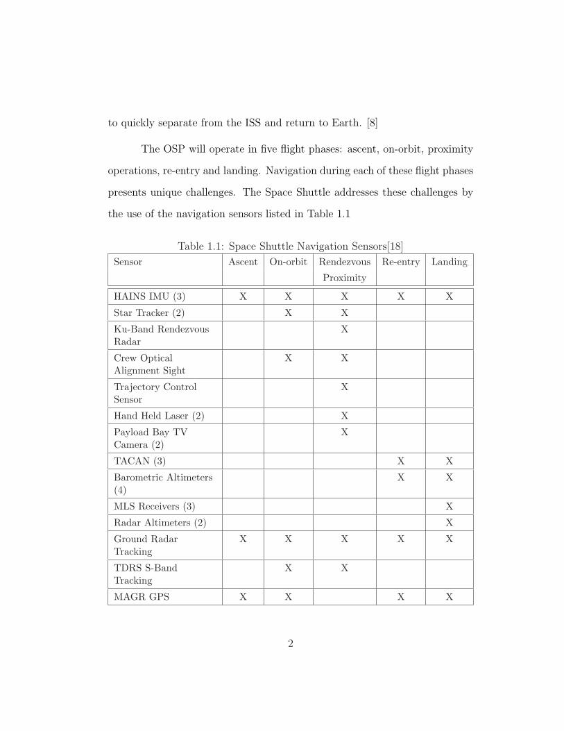
The OSP will operate in five flight phases: ascent, on-orbit, proximity

operations, re-entry and landing. Navigation during each of these flight phases

presents unique challenges. The Space Shuttle addresses these challenges by

the use of the navigation sensors listed in Table 1.1

Table 1.1: Space Shuttle Navigation Sensors[18]

Sensor Ascent On-orbit Rendezvous Re-entry Landing

Proximity

HAINS IMU (3) X X X X X

Star Tracker (2) X X

Ku-Band RendezvousRadar

X

Crew OpticalAlignment Sight

X X

Trajectory ControlSensor

X

Hand Held Laser (2) X

Payload Bay TVCamera (2)

X

TACAN (3) X X

Barometric Altimeters(4)

X X

MLS Receivers (3) X

Radar Altimeters (2) X

Ground RadarTracking

X X X X X

TDRS S-BandTracking

X X

MAGR GPS X X X X

2

Many of these sensors are used only during one or two flight phases.

The complexity, weight, reliability, and power consumption of this suite of

navigation sensors leads to the question: is it possible to design an all flight

phase navigation system with fewer sensors?

A GPS-only navigation system is not adequate because GPS is subject

to outages due to blockage, atmospheric ionization during re-entry, and delta-

v maneuvers. GPS is also subject to errors and integrity problems due to

multipath and other sources. For example, when a spacecraft approaches the

ISS to perform rendezvous and docking, the signals from the GPS satellites

may be blocked by the ISS or degraded by multipath signals reflected by the

ISS.

An unaided inertial navigation system (INS) is not adequate because

the navigation errors of an INS grow without bound over time. The errors

of even today’s most accurate INS systems would become unacceptably large

after several orbits, especially for rendezvous or re-entry.

One possible solution may be to combine GPS with an INS. GPS and

INS are complementary technologies. INS is accurate in the short-term and is

self-contained. GPS is accurate in the long-term but requires access to the GPS

signals. An integrated GPS/INS could take advantage of the strengths of both

systems while minimizing the impact of their weaknesses. The integration of

GPS and INS can be achieved using a Kalman filter, which attempts to find the

optimal navigation solution by proper weighting of the inputs from the GPS

and INS. The Kalman filter could be designed to recognize and adapt itself to

3

the current flight phase, therefore ensuring adequate performance during all

flight phases.

Integrated GPS/INS systems have been used in commercial launch ve-

hicles for the ascent phase. Their performance has been analyzed for the re-

entry and landing phases by Braden, Browning and Gelderloos.[5] GPS/INS

systems have been demonstrated to be capable of precision landing.[14] How-

ever, the performance of GPS/INS systems during remaining flight phases:

on-orbit and proximity operations, has not been completely characterized.

Therefore, the objective of this research is to determine if GPS/INS

navigation during a rendezvous with the ISS is feasible with existing inertial

sensor technology and if not, determine the requirements for future GPS and

inertial sensor technology to make it feasible.

A GPS/INS system is passive and self-contained, requiring only the

availability of GPS signals. Therefore, it can be used during all flight phases.

On the other hand, star trackers and TDRS can typically only be used during

the on-orbit flight phases. Furthermore, since GPS/INS is capable of support-

ing precision landing, it can replace TACAN, MLS receivers, and ground-based

radar, which require extensive support infrastructure on the ground. In ad-

dition to position and velocity information, GPS/INS can provide time and

attitude information. If GPS/INS can be shown to perform adequately for

rendezvous, it would provide a minimum set of sensors capable of navigating

during all mission phases.

4

1.2 Previous Work

The Space Integrated GPS/INS (SIGI) is an example of a spaceborne

integrated GPS/INS system. SIGI is a modified Honeywell H764G Embedded

GPS/INS system which is used on the ISS and was planned to be used on the

Crew Return Vehicle (CRV) before that program was cancelled.[47]

The SIGI flew on seven Space Shuttle missions from September 1997

to December 1999. ISS SIGIs were flown during STS-101 and STS-106 for

the SIGI Orbital Attitude Readiness (SOAR) experiment. The CRV SIGI

was flown on STS-100 and STS-108. The SIGI has been in operational use

on-board the ISS for position, velocity, and attitude since April 2002. How-

ever, the deactivation of Selective Availability and technical issues with the

GPS/INS filter has caused the ISS program to rely on the deterministic GPS-

only position and velocity solution from the embedded Force 19 GPS receiver.

[19]

During re-entry, GPS signals are not available during the “blackout re-

gion” because the air molecules around the vehicle become ionized, interfering

with radio signals. The SIGI was tested during the entire de-orbit and landing

on STS-100 and STS-108. During STS-100, the GPS receiver was not aided

and the GPS receiver dead-reckoned through the blackout region. The receiver

started tracking less than four GPS satellites at 240,000 feet and did not reac-

quire until 130,000 feet. The total time with less than four GPS satellites was

16 minutes. During STS-108, the GPS receiver was inertially aided and reac-

quired at 210,000 feet for a total time with less than four GPS satellites of six

5

minutes, demonstrating the benefit of integrating GPS and INS technology.

[17]

Much work has been done on integrated GPS/INS systems for aircraft

and missiles. There are many examples of these systems in operation today,

such as the Honeywell H764G Embedded GPS/INS, which is currently being

flown in several military aircraft and has been shown to be capable of precision

approach and landing by Elchynski.[14]

Ebinuma demonstrated the use of GPS-only navigation for rendezvous.

He developed an extended Kalman filter to perform real-time relative naviga-

tion and used a hardware-in-the-loop test facility, which integrates navigation

and guidance for rendezvous. However, his models assumed that GPS was

always available and did not include multipath or blockage of the GPS signals.

[13]

The recent research on navigation during proximity operations con-

ducted by Um examined spacecraft relative navigation using an integrated

GPS/INS in the vicinity of the ISS. [41] The GPS/INS was a loosely coupled

system, which included two Kalman filters, one to process the GPS measure-

ments and the other to combine the INS measurements with the output of the

GPS filter. The INS part of the system was simulated in software and the

GPS measurements were collected from a Mitel Architect GPS receiver being

stimulated by a Spirent STR4760 GPS simulator.

6

1.3 Research Contributions

The primary objective of this research is to evaluate the ability of an

integrated GPS/INS to provide accurate navigation solutions during a ren-

dezvous scenario where the effects of ISS signal blockage, multipath and delta-

v maneuvers degrade GPS navigation. In order to accomplish this, models for

an INS operating in orbit, ISS signal blockage and multipath have been devel-

oped and incorporated into a simulation of a GPS/INS during rendezvous.

1.3.1 INS Error Model

An error model for an INS operating in orbit has been developed. This

model has been used to provide the first known characterization of the behavior

on an INS in orbit, which is provided in Appendix A. This characterization can

be used to understand how inertial sensor errors affect navigation performance

in space.

Another contribution is the development of an algorithm for generating

simulated accelerometer and gyro measurements incorporating all significant

error sources. This is the first known publicly available description of such an

algorithm.

1.3.2 ISS Signal Blockage Model

This study is the first known analysis of the effects of the ISS blocking

GPS signals on GPS navigation near the ISS. The ISS is modelled as a sphere,

which given the receiver’s position at an instant of time, creates a cone where

7

GPS signals are blocked. While the ISS is not spherical and GPS signals are

expected to be received within the blockage cone, they may be so degraded by

multipath that it is prudent for GPS receivers to not use any measurements

coming from the area of the blockage cone.

1.3.3 ISS Multipath Model

A new statistical multipath model for spacecraft operating near the ISS

has been developed based on terrestrial urban and indoor multipath models.

The Friis transmission and bi-static radar equations have been used to estimate

parameters that normally are determined by experimental measurements of the

multipath environment. The model characterizes the multipath environment

in terms of the amplitudes, time delays and phases of the multipath signals,

which are used by the C/A code and carrier phase measurement error models

to determine the error in the GPS range measurements.

1.3.4 GPS/INS Extended Kalman Filter Design and Analysis

A complementary extended Kalman filter (EKF) for combining GPS

and INS measurements has been developed. The INS measurements provide

the reference trajectory for the EKF, which computes corrections to the ref-

erence trajectory. The reference trajectory is updated with these corrections

each filter cycle. Both absolute and relative navigation filters have been de-

veloped.

During the development of the absolute navigation filter, the navigation

8

results of using GPS C/A code measurements were compared to those resulting

from the use of GPS carrier phase measurements. For absolute navigation,

it was determined that while GPS carrier phase measurements were more

precise than C/A code measurements, the navigation accuracy was actually

better using C/A code measurements. The reason for this is that in the case

of absolute navigation, the filter was not able to adequately allocate errors

between ionospheric delay, GPS SV clock and ephemeris errors, and the integer

ambiguity.

One of the decisions to be made in the development of a GPS relative

navigation system is whether to exchange measurement data or processed state

data. In order to examine this issue, the absolute navigation filter was run

for both the chaser and ISS and their states were differenced to provide a

relative navigation state. These results were compared to the output of the

relative navigation filter which processed measurements from both the chaser

and ISS. The comparison showed about an order of magnitude improvement

in accuracy when using the relative navigation filter, demonstrating the value

of exchanging measurement data rather than processed state data for relative

navigation.

The inertial sensors come into play mostly during the final phase of

rendezvous, where GPS signals are blocked and are subject to multipath and

many small delta-v and attitude maneuvers that degrade the GPS navigation

performance. To demonstrate the value of the INS during this time, a high-

fidelity rendezvous simulation was developed which includes an algorithm for

9

computing delta-v maneuvers to create a decelerating glideslope trajectory.

The results of a GPS-only relative navigation filter, the GPS/INS relative

navigation filter with the SIGI inertial sensors, and the GPS/INS relative

navigation filter with improved inertial sensors were analyzed and compared.

1.3.5 Rendezvous Simulation and Navigation Design Tool

One of the contributions of this research is a high-fidelity GPS/INS

rendezvous simulator. This simulator provides an accurate simulation of a

Space Shuttle-ISS rendezvous scenario, including the effects of atmospheric

drag, gravity perturbations, and finite duration burns computed by a ren-

dezvous guidance algorithm. The GPS constellation and receiver models in-

clude all significant GPS errors sources for spacecraft in orbit in order to

generate pseudorange and carrier phase measurements. The INS error model

includes all significant INS error sources to generate accelerometer and gyro

measurements.

The simulation can be used to perform trade studies and design anal-

yses for many aspects of GPS and GPS/INS navigation for spacecraft, such

as GPS antenna location and field of view, rendezvous approach direction,

inertial sensor performance, multipath mitigation techniques, and navigation

algorithms.

The simulation is part of the Java Astrodynamics Toolkit (JAT), an

open source software project. Since JAT is licensed under the GNU General

Public License and there are a number of freely available Java development

10

environments, anyone with a computer and an Internet connection can access

the source code. The JAT project is located on the Internet at: http://jat.

sourceforge.net.

1.4 Overview

This section provides an overview of the remaining chapters of this

dissertation.

Chapter 2 describes the coordinate and time systems used in this re-

search and also describes how vectors are transformed from one coordinate

system into another.

Chapter 3 provides a description of the GPS measurement models, in-

cluding the ISS signal blockage and multipath models. The results of the

blockage and multipath simulations are also presented.

Chapter 4 provides a brief introduction into inertial navigation and

describes how the INS error model equations are derived.

Chapter 5 describes the GPS/INS integration architecture, Kalman

filter equations, filter models, and a description of the GPS/INS simulation

including the methods and models used to generate the true rendezvous tra-

jectories, the INS measurements and the GPS measurements.

Chapter 6 presents the results and analysis of the GPS/INS simulations.

Chapter 7 summarizes the research, states conclusions and lists topics

for possible future work.

11

Chapter 2

Coordinate and Time Systems

2.1 Reference Frames

According to Britting, navigation is the determination of a body’s po-

sition and velocity relative to a reference frame.[6] Therefore, the precise def-

inition of the reference frames to be used is fundamental to the navigation

process.

An inertial reference frame is one where Newton’s laws of motion apply.

The origin of such a reference frame must be non-accelerating and the frame

must be non-rotating. In practice, a truly inertial reference frame cannot be

defined in the vicinity of the solar system due to the gravitational fields of all

of the planets and other bodies orbiting the sun. However, it is possible to

define reference systems that are “inertial enough” so that the deviation of

the actual motion of an object from the motion predicted by Newton’s laws is

insignificant over the time span of interest.

Inertial and non-inertial reference frames will be used. The following

reference frames will be described in the next sections: Earth Centered Inertial,

Earth Centered Earth Fixed, Spacecraft Centered, the body frame, and the

navigation frame.

12

2.1.1 Earth Centered Inertial (ECI)

The origin of the ECI system is the center of mass of the Earth. The

fundamental plane is the Earth’s equator with the x-axis pointing towards the

vernal equinox, the y-axis is 90 degrees to the east in the equatorial plane and

the z-axis points to the North Pole. Since the location of the Earth’s equator

and the vernal equinox are time dependent, the ECI frame is not inertial unless

it is fixed at a specified time. The J2000 system represents the best realization

of an ideal, inertial frame at the J2000 epoch. The motion of the equator and

the equinox can be accounted for so inertial frames at other times defined by

the equator and equinox of date can be transformed to the J2000 ECI frame.

These other inertial frames are called true-of-date because they reference the

true equator and true equinox at a particular date. [42]

2.1.2 Earth Centered Earth Fixed (ECEF)

Like the ECI frame, the origin of the ECEF system is at the Earth’s

center of mass and its fundamental plane is the Earth’s equator. The differ-

ence is that it rotates with the Earth. The x-axis is always aligned with the

Greenwich meridian. [42]

2.1.3 Spacecraft Centered (UVW)

The origin of the UVW system is the center of mass of the spacecraft

and moves with the spacecraft. The U -axis lies along the position vector from

the center of mass of the Earth to the spacecraft (radial direction). The V -axis

13

is perpendicular to the x-axis and lies in the direction of motion (along-track

direction). The W -axis completes a right-handed reference system (cross-track

direction). [42]

The basis vectors for the UVW frame can be established at any point

in time by:

U =r

|r| , W =r× v

|r× v| , V = W × U (2.1)

Position vectors or position error vectors can be transformed from the UVW

(B) frame to the ECI (I) frame using the following transformation matrix:

CIB =

[U V W

](2.2)

Velocity vectors or velocity error vectors can be transformed from the ECI

frame to the UVW frame using the velocity rule:

d

dt(r)B =

d

dt(r)I − ωBI × rI (2.3)

where ωBI is the angular velocity of the UVW frame with respect to the ECI

frame.

2.1.4 Body Frame

The body frame is attached to the INS sensor cluster and rotates with it.

In this dissertation, the attitude of the chaser spacecraft and ISS are assumed

to be perfectly maintained so that their respective body frame axes are aligned

with the local UVW frame. The INS sensor cluster and phase center of the

14

GPS antenna are assumed to be located at the spacecraft center of mass. In

a real system, there would be some distance between the spacecraft center of

mass and each sensor, usually referred to as a lever arm. However, no lever

arms are modelled in this dissertation.

2.1.5 Navigation Frame

The navigation frame is the reference frame selected for performing

the inertial navigation computations. For most terrestrial and aircraft appli-

cations, a local geographic frame is selected, however, for an Earth orbiting

spacecraft, the Earth Centered Inertial (ECI) frame is the logical choice for

the navigation frame.

2.1.6 Coordinate Transformations

The transformation of vectors between coordinate systems can be rep-

resented by an orthonormal direction cosine matrix. The direction cosine ma-

trix representing the transformation from coordinate system A to coordinate

system B is denoted by CBA . Vector transformations can also be represented

by quaternions. Both direction cosine matrices and quaternions will be used

throughout this dissertation. The relationship between direction cosine matri-

ces and quaternions is discussed in the next section.

15

2.1.7 Quaternions

In this section, the important quaternion equations are summarized.

More detailed discussions of quaternions can be found in Farrell [15] and Wertz

[45].

A quaternion is a four-parameter set of numbers that can be used to

represent the orientation of a body or reference frame with respect to another

reference frame. Although Euler angles are more intuitively appealing, quater-

nions are free of singularities and are more computationally efficient than Euler

angles or direction cosine matrices. Therefore, strapdown inertial navigation

systems typically use quaternions.

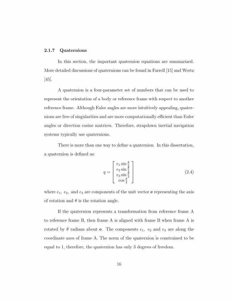
There is more than one way to define a quaternion. In this dissertation,

a quaternion is defined as:

q =

e1 sin θ2

e2 sin θ2

e3 sin θ2

cos θ2

(2.4)

where e1, e2, and e3 are components of the unit vector e representing the axis

of rotation and θ is the rotation angle.

If the quaternion represents a transformation from reference frame A

to reference frame B, then frame A is aligned with frame B when frame A is

rotated by θ radians about e. The components e1, e2 and e3 are along the

coordinate axes of frame A. The norm of the quaternion is constrained to be

equal to 1, therefore, the quaternion has only 3 degrees of freedom.

16

The time derivative of a quaternion can be shown to be: [45]

dq (t)

dt= Ω (ω (t)) q (t) (2.5)

where, ω1, ω2, and ω3 are the components of the instantaneous angular veloc-

ity vector and:

Ω (ω) =1

2

0 ω3 −ω2 ω1

−ω3 0 ω1 ω2

ω2 −ω1 0 ω3

−ω1 −ω2 −ω3 0

(2.6)

Equation (2.6) can also be written as:

dq (t)

dt= Q (q) ω (2.7)

where:

Q (q) =1

2

q4 −q3 q2

q3 q4 −q1

−q2 q1 q4

−q1 −q2 −q3

(2.8)

According to Farrell [15], the quaternion representing a transformation

can be obtained from a direction cosine matrix by the following equations:

q4 =1

2

√1 + C [1, 1] + C [2, 2] + C [3, 3] (2.9)

q =[

C[3,2]−C[2,3]4q4

C[3,2]−C[2,3]4q4

C[3,2]−C[2,3]4q4

q4

](2.10)

It should be noted that (2.10) can become ill-conditioned if q4 ≈ 0. The

equivalent direction cosine matrix can be obtained from a quaternion by the

17

following equation:

C (q) =

q21 − q2

2 − q23 + q2

4 2 (q1q2 − q3q4) 2 (q1q3 + q2q4)2 (q1q2 + q3q4) q2

2 + q24 − q2

1 − q23 2 (q2q3 − q1q4)

2 (q1q3 − q2q4) 2 (q2q3 + q1q4) q23 + q2

4 − q21 − q2

2

(2.11)

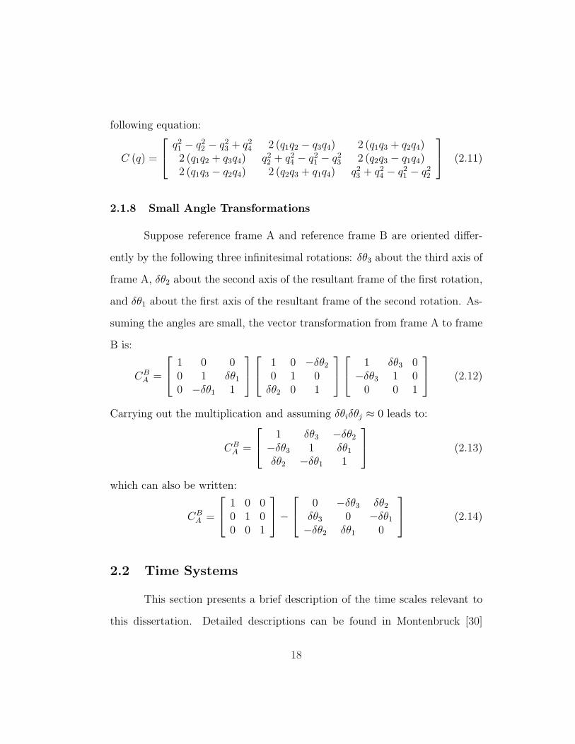
2.1.8 Small Angle Transformations

Suppose reference frame A and reference frame B are oriented differ-

ently by the following three infinitesimal rotations: δθ3 about the third axis of

frame A, δθ2 about the second axis of the resultant frame of the first rotation,

and δθ1 about the first axis of the resultant frame of the second rotation. As-

suming the angles are small, the vector transformation from frame A to frame

B is:

CBA =

1 0 00 1 δθ1

0 −δθ1 1

1 0 −δθ2

0 1 0δθ2 0 1

1 δθ3 0−δθ3 1 0

0 0 1

(2.12)

Carrying out the multiplication and assuming δθiδθj ≈ 0 leads to:

CBA =

1 δθ3 −δθ2

−δθ3 1 δθ1

δθ2 −δθ1 1

(2.13)

which can also be written:

CBA =

1 0 00 1 00 0 1

−

0 −δθ3 δθ2

δθ3 0 −δθ1

−δθ2 δθ1 0

(2.14)

2.2 Time Systems

This section presents a brief description of the time scales relevant to

this dissertation. Detailed descriptions can be found in Montenbruck [30]

18

or Vallado [42]. Relevant time scales include: Terrestrial Time (TT), Inter-

national Atomic Time (TAI), GPS Time, and Coordinated Universal Time

(UTC).

Time can be expressed using various formats such as Julian Date (JD),

Modified Julian Date (MJD), GPS Week Number, and Seconds of the Week.

2.2.1 Time Scales

The fundamental time unit in the International System of Units (SI) is

the SI second. The current definition of the second is based on the resonant

frequency of the cesium atom.

Terrestrial Time is a conceptually uniform time scale which is measured

in days of 86400 SI seconds and is the independent variable of geocentric

ephemerides.

TAI is the practical realization of a uniform time scale based on atomic

clocks and agrees with TT except for a constant offset of 32.184 seconds and

the imperfections of the atomic clocks, such that:

TT = TAI + 32.184 sec (2.15)

GPS Time is an atomic time scale used by the GPS system. It is a

continuous time scale which began at 0 hours on January 6, 1980. GPS Time

is maintained to nominally have a constant offset of 19 seconds from TAI, such

that:

TAI = GPS + 19.0 sec (2.16)

19

UTC is a non-uniform time scale, which is tied to TAI by an integer

number of seconds commonly known as leap seconds. It is updated periodically

to keep UTC in close agreement with mean solar time (UT1) due to variations

in the Earth’s rotation, such that:

TAI = UTC + leap (2.17)

where leap is the integer number of leap seconds between TAI and UTC.

Therefore, UTC is related to GPS Time by:

UTC = GPS + 19.0 sec− leap (2.18)

2.2.2 Time Formats

The Julian Date (JD) is the interval of time in days from noon, January

1, 4713 B.C. Since JD values are typically quite large and begin at noon, it is

convenient to use Modified Julian Date (MJD), which is calculated as follows:

MJD = JD − 2, 400, 000.5 (2.19)

GPS Time is commonly provided in GPS week number and and seconds

of the week. The GPS week number is the number of weeks since the zero

hour, January 6, 1980 GPS epoch, where the first week is assigned a GPS

week number of 0. The GPS week starts on Sunday at zero hours GPS Time.

Within a GPS week, time is given in seconds past the start of the week, yielding

a maximum of 604,800 seconds per week.

20

Chapter 3

GPS Measurement Models

This chapter presents the mathematical models used to simulate the

GPS constellation and to generate simulated GPS measurements. The follow-

ing assumptions are made throughout this dissertation regarding GPS naviga-

tion:

• The chaser spacecraft and ISS each have a single GPS antenna pointed

along the zenith (or radial) direction. The spacecraft is assumed to per-

fectly maintain this orientation and no attitude maneuvers are simulated.

• The GPS antenna fields of view are unobstructed except for the effect

of blockage on the chaser spacecraft due to the ISS and a 10-degree

minimum elevation horizon mask.

• The GPS receivers are either all-in-view receivers or 12-channel receivers

programmed to track the highest elevation GPS satellites.

• The GPS receivers are able to instantly acquire and lock on to new GPS

satellites as they become visible.

• The GPS receivers are L1 single frequency receivers.

21

3.1 GPS Constellation Model

The positions and velocities of the GPS satellites are required in order

to model the GPS measurements. This section presents a description of the

GPS constellation model used in this dissertation and the equations needed to

determine the GPS satellite positions and velocities.

The GPS constellation model was constructed from a daily global broad-

cast ephemeris file in the Receiver Independent Exchange (RINEX) format

obtained from the National Geodetic Survey (NGS) Continuously Operating

Reference Stations (CORS) website. This file contains the GPS broadcast

ephemeris parameters for each satellite in the constellation for March 1, 2001.

There were a total of 28 satellites in the active constellation. The ephemeris

parameters and the equations used to determine the positions of the GPS

satellites at a given time are described below. This GPS constellation model

was used for all simulations in this dissertation.

3.1.1 GPS Ephemeris Parameters

Table 3.1 presents a list of the GPS ephemeris parameters in the broad-

cast navigation message. These parameters can be used to determine the

position and velocity of a GPS satellite.

22

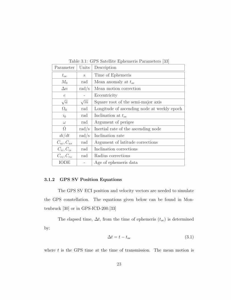
Table 3.1: GPS Satellite Ephemeris Parameters [33]

Parameter Units Description

toe s Time of Ephemeris

M0 rad Mean anomaly at toe

∆n rad/s Mean motion correction

e - Eccentricity√a

√m Square root of the semi-major axis

Ω0 rad Longitude of ascending node at weekly epoch

i0 rad Inclination at toe

ω rad Argument of perigee

Ω rad/s Inertial rate of the ascending node

di/dt rad/s Inclination rate

Cuc, Cus rad Argument of latitude corrections

Cic, Cis rad Inclination corrections

Crc, Crs rad Radius corrections

IODE - Age of ephemeris data

3.1.2 GPS SV Position Equations

The GPS SV ECI position and velocity vectors are needed to simulate

the GPS constellation. The equations given below can be found in Mon-

tenbruck [30] or in GPS-ICD-200.[33]

The elapsed time, ∆t, from the time of ephemeris (toe) is determined

by:

∆t = t− toe (3.1)

where t is the GPS time at the time of transmission. The mean motion is

23

computed using:

n =

√µ

a3+ ∆n (3.2)

where µ = 3.986005 × 1014 m3

s2as defined by the WGS-84 system. Then the

mean anomaly is given by:

M = M0 + n∆t (3.3)

The eccentric anomaly is computed by iteratively solving Kepler’s equation:

M = E − e sin E (3.4)

Kepler’s equation can be solved using the following Newton iteration equation:

En+1 = En +M −Mn

1− e cos En

(3.5)

where:

Mn = En − e sin En (3.6)

The iteration can be initialized by letting E0 = M and finished when M −Mn

becomes acceptably small. The true anomaly is computed by:

ν = tan−1

[sin E

√1− e2/(1− e cos E)

(cos E − e)/(1− e cos E)

](3.7)

The uncorrected argument of latitude is defined as:

u = ν + ω (3.8)

24

The periodic corrections to the radius, argument of latitude and the inclination

can be computed using the following equations:

δr = Crs sin 2u + Crc cos 2u

δu = Cus sin 2u + Cuc cos 2u

δi = Cis sin 2u + Cic cos 2u (3.9)

The corrected orbit elements can be computed using:

r = a(1− e cos E) + δr

u = u + δu

i = i0 + (di/dt)∆t + δi (3.10)

Since the simulation requires a representative GPS constellation and

not the actual GPS constellation at a particular time, the longitude of the

ascending node (measured with respect to the ECEF frame) is treated as

the right ascension of the ascending node (measured with respect to the ECI

frame). This eliminates the need to determine the ECEF to ECI transforma-

tion matrix for a particular date and time. Therefore, the following equation

for right ascension of the ascending node is used:

Ω = Ω0 + Ω∆t (3.11)

The position vector in an orbit frame whose x-axis is pointed toward

the equator is:

rPQW =

r cos ur sin u

0

(3.12)

25

To rotate the position vector into the ECI frame:

rECI = R3(−Ω)R1(−i)rPQW (3.13)

where R3(−Ω) is a rotation about the third axis through an angle of −Ω and

R1 is a rotation about the first axis through an angle of −i.

3.1.3 GPS SV Velocity Equations

The ECI velocity of the GPS SV is the time derivative of the ECI

position given in (3.13), which can be expressed as:

vECI = M(Ω, i)rPQW + M(Ω, i)rPQW (3.14)

where M(Ω, i) = R3(−Ω)R1(−i). Taking the time derivative of (3.12), the

velocity vector in the perifocal plane becomes:

rPQW =

r cos u− ru sin ur sin u + ru cos u

0

(3.15)

where:

r = ae sin EE + δr

δr = 2ν(Crs cos 2u− Crc sin 2u)

u = ν + ˙δu

˙δu = 2ν(Cus cos 2u− Cuc sin 2u) (3.16)

The time derivatives of the eccentric and true anomalies are given by:

E =n

1− e cos E(3.17)

26

and:

ν =n√

1− e2

1 + e cos ν

1− e cos E(3.18)

The time derivative of M is given by:

M(Ω, i) = Ω

− sin Ω − cos i cos Ω sin i cos Ωcos Ω − cos i sin Ω sin i sin Ω

0 0 0

+ (di/dt + δi)

0 sin i sin Ω cos i sin Ω0 − sin i cos Ω − cos i cos Ω0 cos i − sin i

(3.19)

where:

δi = 2ν(Cis cos 2u− Cic sin 2u) (3.20)

3.2 GPS Measurement Equations

This section contains the equations for the GPS pseudorange and carrier

phase measurements. Detailed discussions of the GPS measurement equations

can be found in Hofmann-Wellenhof [21] and Ebinuma [13].

3.2.1 Pseudorange Measurement

Let tS be the reading on the satellite clock at the time the signal is sent

and tR be the reading on the receiver clock at the time the signal is received.

Both clocks are in error with respect to GPS system time, so that:

tR = tR(GPS) + ∆tR (3.21)

tS = tS(GPS) + ∆tS (3.22)

27

where tR(GPS) and tS(GPS) are the true GPS system times of receipt and

transmission, and ∆tR and ∆tS are the receiver and GPS satellite clock errors,

respectively.

The measured pseudorange is given by:

P (tR) = c(tR − tS) (3.23)

where c is the speed of light. Substituting (3.21) and (3.22) into (3.23) for the

following expression yields the pseudorange equation:

P (tR) = c(tR(GPS)− tS(GPS))− c(∆tR −∆tS) (3.24)

The geometric distance the signal travelled from transmission at the GPS

satellite to reception at the receiver is:

ρ(tR(GPS)) = c(tR(GPS)− tS(GPS)) (3.25)

However, the receiver provides the pseudorange measurement at time tR, not

at tR(GPS). Since the true GPS system time is unknown, the geometric

distance is linearized about the known receiver measured time using a Taylor

series, such that:

ρ(tR(GPS)) = ρ(tR −∆tR) ≈ ρ(tR)− ρ(tR)∆tR (3.26)

where second order and higher terms are ignored. Substituting (3.26) into

(3.24) yields the pseudorange measurement equation:

P (tR) ≈ ρ(tR) + (c− ρ(tR))∆tR − c∆tS (3.27)

28

3.2.2 Range Rate Equation

According to Ebinuma, the range rate contributes less than 1 mm to

the range measurement for a stationary receiver on the ground with a receiver

clock bias less than 1 msec. [13] Therefore, this small contribution is generally

neglected for stationary terrestrial applications. However, this is not true for

spacecraft in low Earth orbit.

The line of sight vector from the receiver to the jth GPS satellite is

defined as:

ρj = rGPSj(tS)− r(tR) (3.28)

The relative velocity between the receiver and the jth GPS SV can be defined

as:

vrelj = vGPSj(tS)− v(tR) (3.29)

where vGPSjis the velocity of the GPS SV and v is the velocity of the receiver.

Then, the following equation for the instantaneous range rate of the jth GPS

SV can be used: [13]

ρj (tR) =ρj · vrelj

ρj (tR) + ρj · (vGPSj(tS)/c)

(3.30)

3.2.3 Carrier Phase Measurement

The GPS carrier phase measurement is somewhat similar to the pseu-

dorange measurement except that instead of measuring the time it takes for

the signal to travel from the GPS satellite to the receiver, the receiver measures

29

the difference in the carrier phase between the receiver and the phase of a ref-

erence carrier. The measurement contains no information about the number

of whole cycles. This is referred to as the integer ambiguity. The scaled carrier

phase measurement equation differs from the pseudorange equation only by

the integer ambiguity N multiplied by the GPS wavelength λ:

λΦ(tR) ≈ ρ(tR) + (c− ρ(tR))∆tR − c∆tS + λN (3.31)

3.2.4 Satellite Motion During Signal Propagation

The true distance from the GPS satellite at the time of transmission

to the receiver at the time of reception ρ(tR) is a function of two time epochs.

Therefore, the motion of the GPS satellite during the signal travel time must

be accounted for. An iterative scheme is used to solve for the time of signal

transmission. The iteration is initialized by:

tS0 = tR (3.32)

The equation for the next estimate of the time of transmission is:

tSn+1 = tR +

∥∥rGPS(tSn)− r(tR)∥∥

c(3.33)

where rGPS(tSn) is the GPS SV position vector computed using (3.13) for the

nth approximation tSn and r(tR) is the receiver position vector at tR. The

iteration is continued until:

∣∣tSn+1 − tSn∣∣ < ε (3.34)

30

where ε is a small error tolerance. The true geometric distance for the jth

GPS SV can then be computed by:

ρj(tR) =∥∥rGPSj

(tS)− r(tR)∥∥ (3.35)

3.3 GPS Measurement Error Models

The GPS measurement error models for pseudorange, carrier phase,

and single difference carrier phase measurements are presented in this section.

3.3.1 Pseudorange and Carrier Phase

Ideally, the GPS receiver would measure the true range to the GPS SV,

however, the pseudorange and carrier phase measurements are biased and noisy

measurements. The errors included in the GPS measurement model include:

receiver and SV clock biases, GPS SV ephemeris errors, ionospheric delays,

multipath errors and random measurement noise. Therefore, the pseudorange

and carrier phase measurements models can be expressed as:

P (t) = ρ + [c− ρ] ∆tR − c∆tS + ∆URE + ∆iono + ∆mp + εpr (3.36)

λΦ(t) = ρ + [c− ρ] ∆tR − c∆tS + ∆URE + ∆iono + ∆mp + λN + εcp

where:

∆URE = user range error

∆iono = ionospheric delay range error

∆mp = multipath range error

31

εpr = pseudorange measurement error

εcp = carrier phase range measurement error

The user range error is caused by errors in the broadcast ephemerides

and GPS SV clock corrections. Tropospheric delay is not included because

both the chaser spacecraft and ISS are assumed to be above the troposphere.

Also, since Selective Availability (SA) was turned off on May 1, 2000, SA clock

dither and ephemeris errors are not included.

3.3.2 Single Difference Carrier Phase

If two spacecraft are close enough that the signal path from each GPS

SV is almost the same, the GPS SV related errors such as ionospheric delay,

GPS SV clock, and ephemeris errors are cancelled out when the difference

between measurements from the two spacecraft is taken. If simultaneous mea-

surements from the two spacecraft (denoted by the subscripts A and B) with

the same GPS SV exist, then the single difference carrier phase measurement

for the j th GPS SV can be defined by:

λΦjAB = ρj

AB + ρjA∆tA − ρj

B∆tB + c(∆tB −∆tA) + λN jAB + εj

AB (3.37)

where ∗jAB = ∗j

B − ∗jA. If the measurements are statistically independent, the

variance of the measurement noise is doubled when taking the difference of

two carrier phase measurements.

The measurements from both vehicles are assumed to be taken simul-

taneously and instantly received by the chaser vehicle. In the real world, the

32

d i r e c ts i g n a l

r e f l e c t e dr a y s

b l o c k e ds i g n a l

Figure 3.1: The ISS Blockage and Multipath Scenario

difference between the measurement times and the transmission delay would

have to be accounted for. One means of assuring that the measurements are

taken simultaneously would be to steer the receiver clocks to track GPS time.

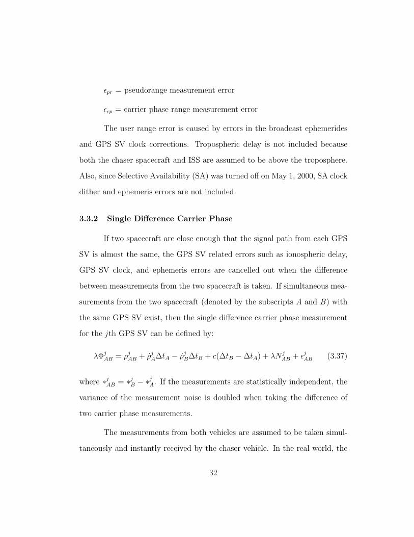
3.4 ISS Blockage and Multipath Models

For spacecraft operating in the vicinity of the ISS, GPS signals can

be blocked or degraded by multipath signals being reflected off of the ISS as

shown in Figure 3.1.

3.4.1 ISS Signal Blockage Model

It has been hypothesized that the ISS will block GPS signals needed

by other spacecraft to navigate during rendezvous operations. To analyze this

33

X

Y

Z

I S S

G P S

C H A S E R

r G P S

r

r j

r I S S

r I S S

r G PS /

I S S

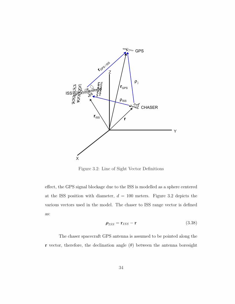
Figure 3.2: Line of Sight Vector Definitions

effect, the GPS signal blockage due to the ISS is modelled as a sphere centered

at the ISS position with diameter, d = 100 meters. Figure 3.2 depicts the

various vectors used in the model. The chaser to ISS range vector is defined

as:

ρISS = rISS − r (3.38)

The chaser spacecraft GPS antenna is assumed to be pointed along the

r vector, therefore, the declination angle (θ) between the antenna boresight

34

and the GPS line of sight vector can be found by:

cos θj =r · ρj

r ρj

(3.39)

where r = ‖r‖ and ρj = ‖ρj‖.

The region of GPS signal blockage is defined by a cone about the chaser

to ISS range vector. The central angle of the cone, γ, is determined by the

radius of the blockage sphere and the distance from the chaser to the ISS as

follows:

tan(γ) =d/2

ρISS

(3.40)

where ρISS = ‖ρISS‖.

The angle between the GPS line of sight vector and the chaser to ISS

range vector is found by:

cos χj =ρISS · ρj

ρISS ρj

(3.41)

If the angle χj is less than γ, the GPS signal would be within the

blockage cone and considered to be blocked. Additionally, any GPS signals

below a 10 minimum elevation angle from the horizonal plane, perpendicular

to the antenna boresight vector, are also considered to be blocked. A side view

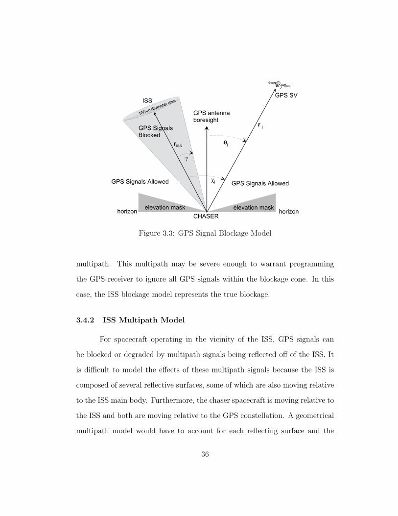
of the GPS signal blockage model is shown in Figure 3.3. The shaded areas

represent the regions where the GPS signals are blocked.

While the ISS is not actually a sphere and GPS signals will be received

from within the sphere, it is likely that those signals will be corrupted by

35

G P S a n t e n n ab o r e s i g h t

h o r i z o n h o r i z o ne l e v a t i o n m a s ke l e v a t i o n m a s k

G P S S i g n a l s A l l o w e dG P S S i g n a l s A l l o w e d

G P S S V

q j

G P S S i g n a l sB l o c k e d

r j

r I S S

g

c j

C H A S E R

I S S

Figure 3.3: GPS Signal Blockage Model

multipath. This multipath may be severe enough to warrant programming

the GPS receiver to ignore all GPS signals within the blockage cone. In this

case, the ISS blockage model represents the true blockage.

3.4.2 ISS Multipath Model

For spacecraft operating in the vicinity of the ISS, GPS signals can

be blocked or degraded by multipath signals being reflected off of the ISS. It

is difficult to model the effects of these multipath signals because the ISS is

composed of several reflective surfaces, some of which are also moving relative

to the ISS main body. Furthermore, the chaser spacecraft is moving relative to

the ISS and both are moving relative to the GPS constellation. A geometrical

multipath model would have to account for each reflecting surface and the

36

relative motion between the ISS, chaser spacecraft and GPS satellites. This

would be computationally intensive and not practical for some applications,

such as an integrated GPS/INS navigation simulation of a rendezvous scenario.

Therefore, a statistical multipath model was selected instead of a geometrical

multipath model.

The following assumptions are made in formulating this model:

1. If a GPS signal is not blocked by the ISS, it is subject to multipath.

2. For each GPS signal that is not blocked by the ISS, many reflections are

caused and there is no single dominant reflector.

3. The phases of the reflections are uniformly distributed over the angle [0,

2π). The rationale for this assumption is explained later in this chapter.

4. The relative velocity between the chaser spacecraft and the ISS is small,

so that there is no relative Doppler effect between the direct and reflected

signals.

According to Comp, an electromagnetic signal may reach an antenna by

a single direct path or indirectly through one or more reflected paths. Because

of the extra path length they travel, multipath signals usually arrive at the

antenna with a delay relative to the direct signal. For GPS carrier phase

measurements, multipath signals combine with the direct signal to distort the

received phase.[11] Assuming that there are multiple reflections, each reflected

path has an associated propagation delay and attenuation factor. Both the

37

propagation delays and attenuation factors are time varying due to the relative

motion and geometry of the vehicles.

Consider the transmission of an unmodulated carrier at frequency fc.

The transmitted signal can be expressed as:

x (t) = A0ej(2πfct) (3.42)

The multipath channel consists of multiple paths or rays that have real

positive gains βk, propagation delays τk and phase shifts θk, where k is the path

index and in principle ranges from 0 to ∞. The complex, low-pass channel

impulse response is given as:[35]

h (t) =∞∑

k=0

βk ejθkδ (t− τk) (3.43)

where δ (·) is the Dirac delta function. The composite received signal is the

time convolution of x (t)and h (t) and can be represented as:[35]

rc (t) =∞∑

k=0

A0 βk ej2π fc(t−τk)+θk (3.44)

If the direct path term is separated out and the range of k is limited to

a finite number N of multipath rays, the composite received signal becomes:

rc (t) = A0 β0 ej2π fct +N∑

k=1

A0 βk ej2π fc(t−τk)+θk (3.45)

If the direct signal phase is defined as φd = 2πfct and the multipath

relative phase shift of the kth ray is defined as ψk = 2πfcτk + θk, then the

38

composite received signal can be expressed as:

rc (t) = A0 β0 ej φd +N∑

k=1

A0 βk ej(φd+ψk) (3.46)

3.4.3 GPS Carrier Phase Measurement Errors

The error in the carrier phase measurement, δφ, due to multipath can

is given by:[1]

tan δφ =

N∑k=1

A0 βk sin ψk

A0 β0 +N∑

k=1

A0 βk cos ψk

(3.47)

where A0 represents the amplitude of the signal transmitted by the GPS satel-

lite. Factoring out A0 leaves:

tan δφ =

N∑k=1

βk sin ψk

β0 +N∑

k=1

βk cos ψk

(3.48)

3.4.4 GPS C/A Code Measurement Errors

The error due to multipath in GPS C/A code measurements for a non-

coherent GPS receiver has been derived by Braasch [4]. An approximation of

the code correlation function is:

R(τ) =

1− |τ |

T|τ | ≤ T

0 |τ | > T(3.49)

where T is the PRN code bit period. The normalized form of the discriminator

39

function with a single multipath ray is given by:[4]

D(τ) = R2(τ + τd)−R2(τ − τd)+

α2[R2(τ + τd + τm)−R2(τ − τd + τm)]+

2α cos(ψm)[R(τ + τd)R(τ + τd + τm)−

R(τ − τd)R(τ − τd + τm)] (3.50)

where τ is the delay lock loop (DLL) tracking error, α is the multipath relative

amplitude, τm is the multipath relative time delay and ψm is the multipath

relative phase angle. The τ corresponding to the zero-crossing of the discrim-

inator function is the DLL tracking error caused by multipath, which is equal

in magnitude but opposite in sign of the ranging error due to multipath.

Mora-Castro, et al, extended this equation to include the effects of

multiple multipath rays. In this case, the discriminator function is given by:[31]

D(τ) = R2(τ + τd)−R2(τ − τd)

+ 2N∑

k=1

αk cos(ψk)[R(τ + τd)R(τ + τd + τk)−R(τ − τd)R(τ − τd + τk)]

+N∑

k=1

N∑

l=1

αkαl cos(ψk−ψl)[R(τ+τd+τk)R(τ+τd+τl)−R(τ−τd+τk)R(τ−τd+τl)]

(3.51)

where:

αk =βk

β0

(3.52)

40

3.4.4.1 Conjectures

Some conjectures about the nature of multipath signals have been used

because there is limited spaceflight experiment data available. These conjec-

tures are based on terrestrial multipath models and measurements. Conjec-

tures about the relative phase shifts, relative amplitudes, the multipath power

delay profile and relative time delays are described in this section.

Phase Shifts. The multipath relative phase angle ψk changes by 2π when the

path length changes by one wavelength. For the GPS L1 signal, fc =1575.42

MHz, the wavelength is about 19 cm. This implies that small motions of the

reflector or receiver can cause ψk to change by 2π. The delays associated

with different paths are expected to change at different rates and in an unpre-

dictable or random manner. If one considers a fixed transmitter and a mobile

receiver, and imagines an ensemble of receiver positions spread over hundreds

or thousands of wavelengths, then the geometry of a single path with delay

τk will lead to a uniform distribution of phase for that path, while the ge-

ometrical relationship between separate paths with different delays will lead

to a uniform joint distribution of pairs of phases, thus the phases would be

independent. Therefore, the phase angles will be assumed to be statistically

independent random variables with a uniform distribution over the range [0,

2π). [35]

Amplitudes. The received multipath signals can be modelled as random

processes. When there are a large number of paths (in practice, greater than

6), the central limit theorem may be applied so that the received signal may

41

be modelled as a complex-valued Gaussian random process.[35]

The received signal can be broken down into in-phase and quadrature

components, I(t) and Q(t), which are independent Gaussian processes. This

means that they are completely characterized by their mean value and auto-

correlation function. I(t) and Q(t) have equal variance σ2 equal to the mean

square power. The total amplitude of the signal is the square root of the sum

of the squares of I(t) and Q(t), which are Gaussian. This leads to the con-

jecture that the amplitudes are Rayleigh distributed. Therefore, the βk’s are

Rayleigh distributed such that:

p(β2

k

)=

1

β2k

e−

(β2

k/β2k

)

(3.53)

where β2k= the average power gain at τk.[38]

Power Delay Profile. The multipath power-delay profile for a given en-

vironment is the expected power received as a function of delay. Numerous

measurements of the multipath power-delay profile for various environments

have been made, such as those by Van Rees[44] and Belloul[2]. Based on these

studies, a general model of the multipath average power delay profile can be

given as:[43]

P (τ) = P0 e−τ/τ (3.54)

where τ is the mean excess delay of the multipath reflections and P0 is the

total multipath power. The total multipath power is estimated by using the

42

bi-static radar equation:

P0 =ARCS λ2Gmp

r Pt Gt

(4π)3 ρISS2 r2

GPS/ISS

(3.55)

where ρISS is the distance from the chaser to the ISS, rGPS/ISS is the distance

from the ISS to the GPS satellite, ARCS is the radar cross sectional area of

the ISS, λ is the wavelength, Gmpr is the antenna gain of the receiver in the

direction of the multipath, and Pt Gt is the effective isotropic radiated power

from the GPS satellite.

The average power in each multipath signal is:

Pk =1

2A2

0 β2k (3.56)

Equating this with equation (3.54) and solving for β2k leads to:

β2k =

2P0

A20

e−τ/τ (3.57)

Substituting (3.55) into (3.57) and recognizing that A20 = 2Pt Gt results in the

following expression:

β2k (τ) =

ARCS λ2Gmpr

(4π)3 ρISS2 r2

GPS/ISS

e−τ/τ (3.58)

Since the multipath rays are being reflected off of the ISS, the mean excess

delay is approximated by:

τ =ρISS

c(3.59)

43

where c is the speed of light. The power of the direct signal is estimated by

using the Friis equation:

Pdirect =1

2A2

0 β20 =

λ2Gdirectr Pt Gt

(4πρj)2 (3.60)

Since A20 = 2Pt Gt,

β20 =

λ2Gdirectr(

4πrGPS/STS

)2 (3.61)

If a cardioid pattern antenna is used, then:

Gdirectr = 1 + cos θdirect (3.62)

where θdirect is the angle between the direct line of sight vector and the antenna

boresight vector. Substituting (3.62) into (3.61) leads to:

β0 =

√λ2 (1 + cos θdirect)

(4πρj)2 (3.63)

Delay Times. The mean excess delay and RMS delay spread are commonly

used to characterize multipath time delays. The parameters are determined

from a multipath power delay profile. The mean excess delay is the first

moment of the power delay profile and is defined to be:[36]

τ =

∑k

β2k τk

∑k

β2k

(3.64)

Turin, et al, proposed that the delay times form a Poisson sequence.[40]

The probability distribution of time delays is given by:[25]

p (τk) =1

τe−

τkτ (3.65)

44

3.4.4.2 Multipath Model Algorithm

This section describes how the multipath error for each GPS carrier

phase measurement is computed for the simulation. The algorithm is:

1. For each simulation time and each GPS satellite, compute: r, rGPS/ISS

and θdirect.

2. Compute β0 using (3.63) and τ using (3.59).

3. Given N , obtain the τk’s from the Poisson distribution given in (3.65).

4. For each τk:

• Given ARCS, compute β2k using (3.58).

• Obtain the βk’s from the Rayleigh distribution given in (3.53).

• Obtain the ψk’s from a uniform distribution over [0, 2π).

• Construct βk sin ψk and βk cos ψk

5. Determine the carrier phase range error from (3.48).

6. Determine the code range error from (3.51)

A flowchart of the combined ISS blockage and multipath models is

shown in Figure 3.11 which is located at the end of the chapter.

45

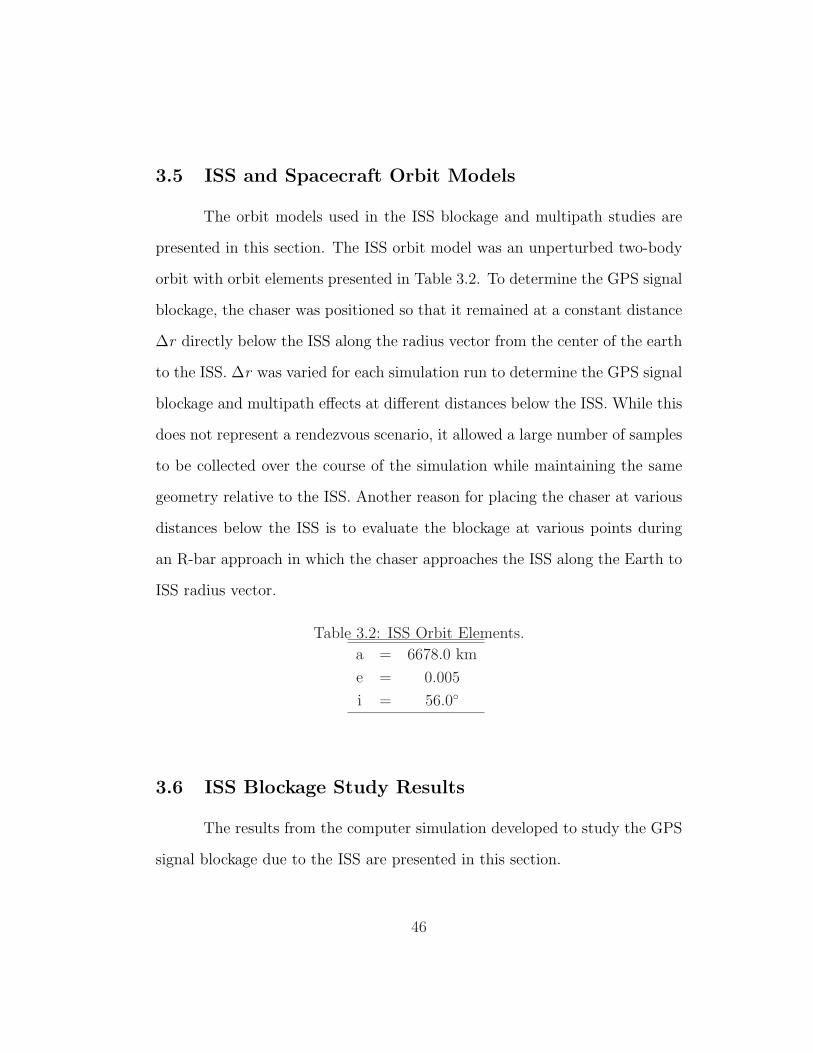
3.5 ISS and Spacecraft Orbit Models

The orbit models used in the ISS blockage and multipath studies are

presented in this section. The ISS orbit model was an unperturbed two-body

orbit with orbit elements presented in Table 3.2. To determine the GPS signal

blockage, the chaser was positioned so that it remained at a constant distance

∆r directly below the ISS along the radius vector from the center of the earth

to the ISS. ∆r was varied for each simulation run to determine the GPS signal

blockage and multipath effects at different distances below the ISS. While this

does not represent a rendezvous scenario, it allowed a large number of samples

to be collected over the course of the simulation while maintaining the same

geometry relative to the ISS. Another reason for placing the chaser at various

distances below the ISS is to evaluate the blockage at various points during

an R-bar approach in which the chaser approaches the ISS along the Earth to

ISS radius vector.

Table 3.2: ISS Orbit Elements.

a = 6678.0 km

e = 0.005

i = 56.0

3.6 ISS Blockage Study Results

The results from the computer simulation developed to study the GPS

signal blockage due to the ISS are presented in this section.

46

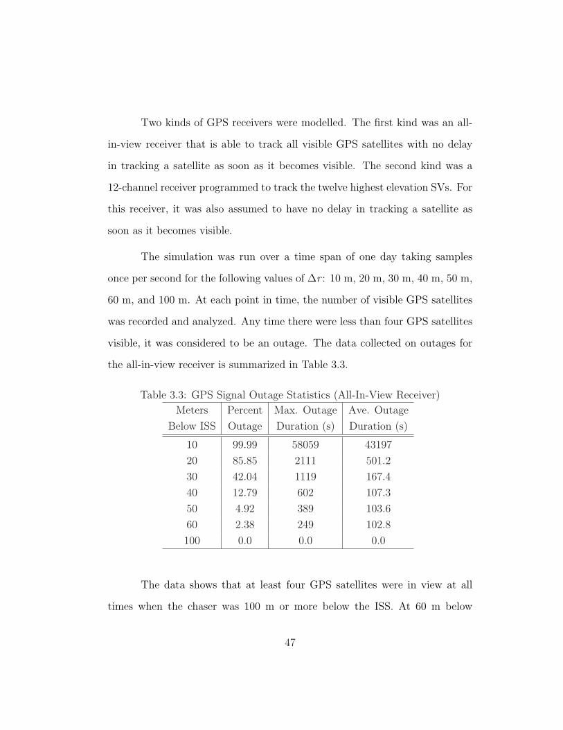
Two kinds of GPS receivers were modelled. The first kind was an all-

in-view receiver that is able to track all visible GPS satellites with no delay

in tracking a satellite as soon as it becomes visible. The second kind was a

12-channel receiver programmed to track the twelve highest elevation SVs. For

this receiver, it was also assumed to have no delay in tracking a satellite as

soon as it becomes visible.

The simulation was run over a time span of one day taking samples

once per second for the following values of ∆r : 10 m, 20 m, 30 m, 40 m, 50 m,

60 m, and 100 m. At each point in time, the number of visible GPS satellites

was recorded and analyzed. Any time there were less than four GPS satellites

visible, it was considered to be an outage. The data collected on outages for

the all-in-view receiver is summarized in Table 3.3.

Table 3.3: GPS Signal Outage Statistics (All-In-View Receiver)

Meters Percent Max. Outage Ave. Outage

Below ISS Outage Duration (s) Duration (s)

10 99.99 58059 43197

20 85.85 2111 501.2

30 42.04 1119 167.4

40 12.79 602 107.3

50 4.92 389 103.6

60 2.38 249 102.8

100 0.0 0.0 0.0

The data shows that at least four GPS satellites were in view at all

times when the chaser was 100 m or more below the ISS. At 60 m below

47

the ISS, there were less than four satellites in view for a small percentage of

the time but the average outage was over 102 seconds long. The amount of

blockage increases as the chaser is brought closer to the ISS. When it is 10 m

below the ISS, no GPS position fixing is possible. These results suggest that

aiding of GPS is required when a chaser spacecraft is within 60 m of the ISS.

The 12-channel receiver results were almost identical to the all-in-view

receiver results. The only difference was that the number of satellites below the

horizon mask was higher for the all-in-view receiver. Therefore, the number

of visible GPS satellites for a 12-channel receiver programmed to select the 12

highest elevation SVs was the same as an all-in-view receiver.

3.7 Multipath Study Results

The multipath model described in this paper was added to the ISS

signal blockage simulation. The carrier phase and code range errors for each

channel of an all-in-view GPS receiver were computed and converted to meters.

Time histories for the carrier phase and code range errors for a single channel

of this receiver were computed for various values of r to determine the behavior

as the chaser approaches the ISS. The values of N and ARCS were also varied

to determine the sensitivity to these two model tuning parameters.

3.7.1 Geometry Dependence

The errors due to multipath are dependent on the GPS satellite geom-

etry because a stronger direct signal is less susceptible to multipath. Higher

48

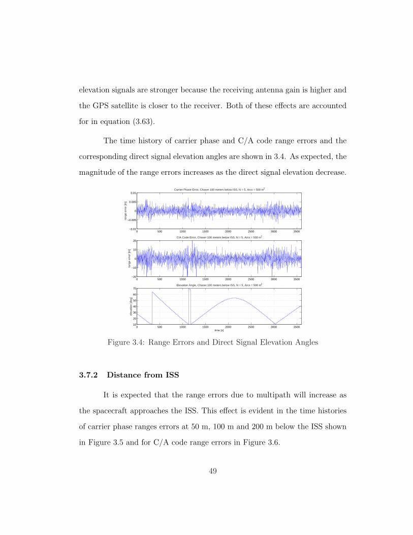
elevation signals are stronger because the receiving antenna gain is higher and

the GPS satellite is closer to the receiver. Both of these effects are accounted

for in equation (3.63).

The time history of carrier phase and C/A code range errors and the

corresponding direct signal elevation angles are shown in 3.4. As expected, the

magnitude of the range errors increases as the direct signal elevation decrease.

0 500 1000 1500 2000 2500 3000 3500−0.01

−0.005

0

0.005

0.01

rang

e er

ror

[m]

Carrier Phase Error, Chaser 100 meters below ISS, N = 5, Arcs = 500 m2

0 500 1000 1500 2000 2500 3000 3500−20

−10

0

10

20

rang

e er

ror

[m]

C/A Code Error, Chaser 100 meters below ISS, N = 5, Arcs = 500 m2

0 500 1000 1500 2000 2500 3000 350010

20

30

40

50

60

70

time [s]

elev

atio

n [d

eg]

Elevation Angle, Chaser 100 meters below ISS, N = 5, Arcs = 500 m2

Figure 3.4: Range Errors and Direct Signal Elevation Angles

3.7.2 Distance from ISS

It is expected that the range errors due to multipath will increase as

the spacecraft approaches the ISS. This effect is evident in the time histories

of carrier phase ranges errors at 50 m, 100 m and 200 m below the ISS shown

in Figure 3.5 and for C/A code range errors in Figure 3.6.

49

0 500 1000 1500 2000 2500 3000 3500−0.02

−0.01

0

0.01

0.02

rang

e er

ror

[m]


0 500 1000 1500 2000 2500 3000 3500−0.02

−0.01

0

0.01

0.02

rang

e er

ror

[m]

Carrier Phaser Error, Chaser 100 meters below ISS, N = 5, Arcs = 500 m2

0 500 1000 1500 2000 2500 3000 3500−0.02

−0.01

0

0.01

0.02

time [s]

rang

e er

ror

[m]


Figure 3.5: Carrier Phase Range Errors at 50m, 100 m and 200 m Below theISS

3.7.3 Number of Multipath Rays

One of the model parameters is the number of multipath rays per GPS

signal. The number of reflected rays would be expected to increase as more

modules, solar arrays and thermal radiators are added to the ISS. It is expected

that the range errors due to multipath will increase as the number of multipath

rays (N) increases. This trend is seen in the time histories of carrier phase

range errors at 100 m below the ISS shown in Figure 3.7 and in C/A code

range errors in Figure 3.8.

50

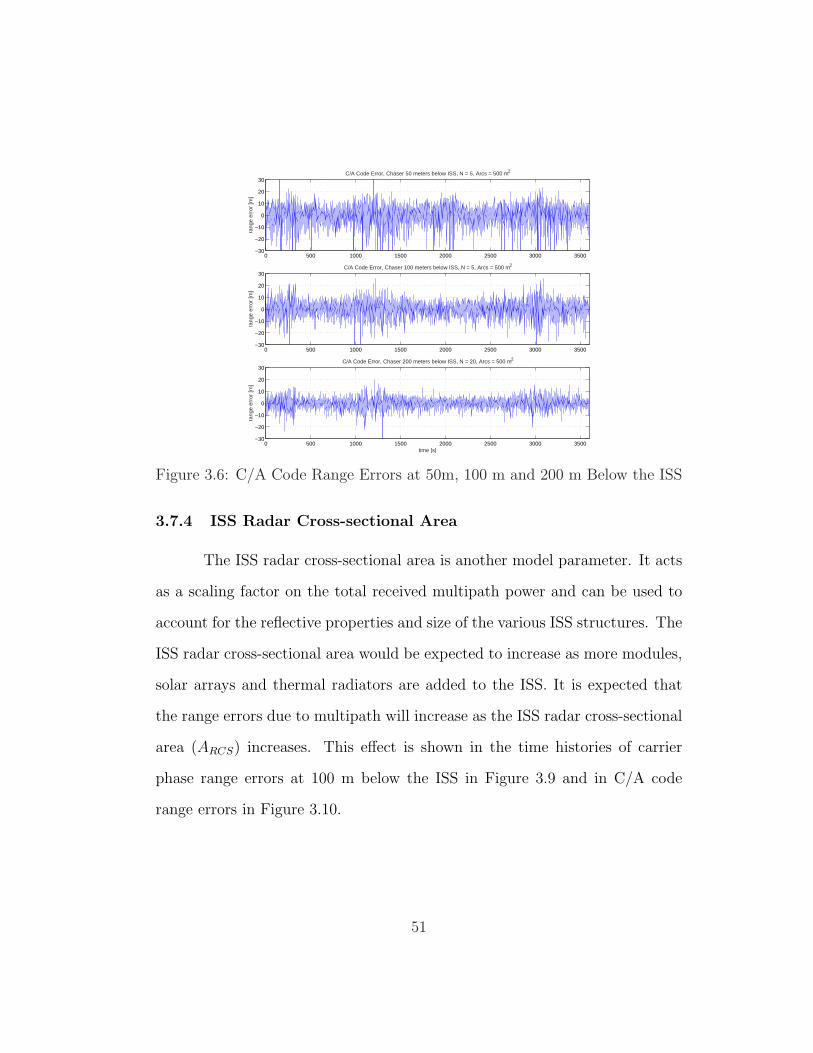
0 500 1000 1500 2000 2500 3000 3500−30

−20

−10

0

10

20

30

rang

e er

ror

[m]


0 500 1000 1500 2000 2500 3000 3500−30

−20

−10

0

10

20

30

rang

e er

ror

[m]


0 500 1000 1500 2000 2500 3000 3500−30

−20

−10

0

10

20

30

time [s]

rang

e er

ror

[m]


Figure 3.6: C/A Code Range Errors at 50m, 100 m and 200 m Below the ISS

3.7.4 ISS Radar Cross-sectional Area

The ISS radar cross-sectional area is another model parameter. It acts

as a scaling factor on the total received multipath power and can be used to

account for the reflective properties and size of the various ISS structures. The

ISS radar cross-sectional area would be expected to increase as more modules,

solar arrays and thermal radiators are added to the ISS. It is expected that

the range errors due to multipath will increase as the ISS radar cross-sectional

area (ARCS) increases. This effect is shown in the time histories of carrier

phase range errors at 100 m below the ISS in Figure 3.9 and in C/A code

range errors in Figure 3.10.

51

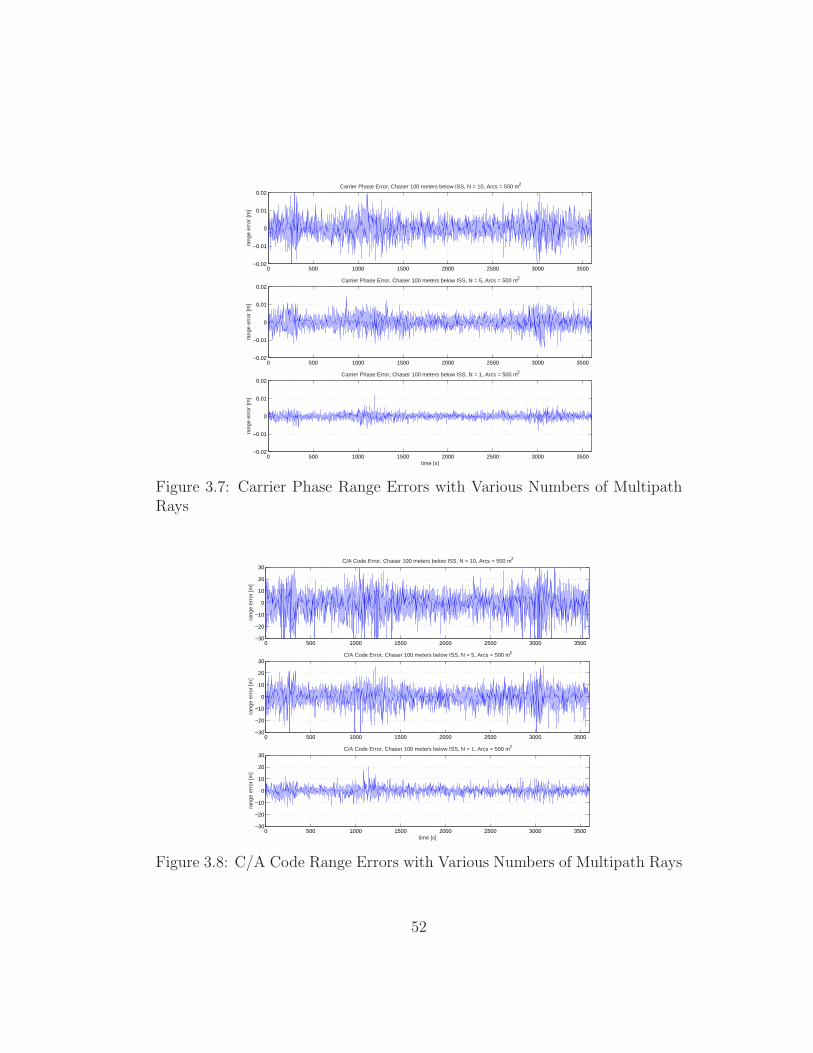
0 500 1000 1500 2000 2500 3000 3500−0.02

−0.01

0

0.01

0.02

rang

e er

ror

[m]


0 500 1000 1500 2000 2500 3000 3500−0.02

−0.01

0

0.01

0.02

rang

e er

ror

[m]


0 500 1000 1500 2000 2500 3000 3500−0.02

−0.01

0

0.01

0.02

time [s]

rang

e er

ror

[m]


Figure 3.7: Carrier Phase Range Errors with Various Numbers of MultipathRays

0 500 1000 1500 2000 2500 3000 3500−30

−20

−10

0

10

20

30

rang

e er

ror

[m]


0 500 1000 1500 2000 2500 3000 3500−30

−20

−10

0

10

20

30

rang

e er

ror

[m]


0 500 1000 1500 2000 2500 3000 3500−30

−20

−10

0

10

20

30

time [s]

rang

e er

ror

[m]


Figure 3.8: C/A Code Range Errors with Various Numbers of Multipath Rays

52

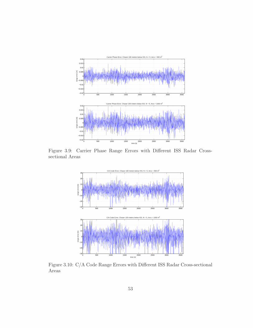
0 500 1000 1500 2000 2500 3000 3500−0.02

−0.015

−0.01

−0.005

0

0.005

0.01

0.015

0.02

rang

e er

ror

[m]


0 500 1000 1500 2000 2500 3000 3500−0.02

−0.015

−0.01

−0.005

0

0.005

0.01

0.015

0.02

time [s]

rang

e er

ror

[m]


Figure 3.9: Carrier Phase Range Errors with Different ISS Radar Cross-sectional Areas

0 500 1000 1500 2000 2500 3000 3500−30

−20

−10

0

10

20

30

rang

e er

ror

[m]


0 500 1000 1500 2000 2500 3000 3500−30

−20

−10

0

10

20

30

time [s]

rang

e er

ror

[m]


Figure 3.10: C/A Code Range Errors with Different ISS Radar Cross-sectionalAreas

53

3.7.5 Model Tuning and Validation

The following parameters can be used to tune the multipath model: the

ISS radar cross-sectional area, the number of multipath reflections per direct

signal, and the direct signal antenna gain.

As more modules, solar arrays and thermal radiators are added to the

ISS, its radar cross-sectional area and the number of multipath reflections are

expected to increase. Therefore, the multipath model can readily adjust to

the changing configuration of the ISS over time.

After consulting with engineers at the NASA Johnson Space Center, it

was determined that the data needed to validate the ISS blockage and mul-

tipath models does not currently exist. Therefore, the values of the tuning

parameters used in the multipath study were chosen based on anecdotal expe-

rience and not on empirical data.

Since engineers are currently designing autonomous rendezvous and

docking systems for the ISS using GPS, it is recommended that a flight ex-

periment to determine the levels of GPS signal blockage and multipath for

pseudorange and carrier phase measurements near the ISS be flown as soon as

possible.

54

!

" #

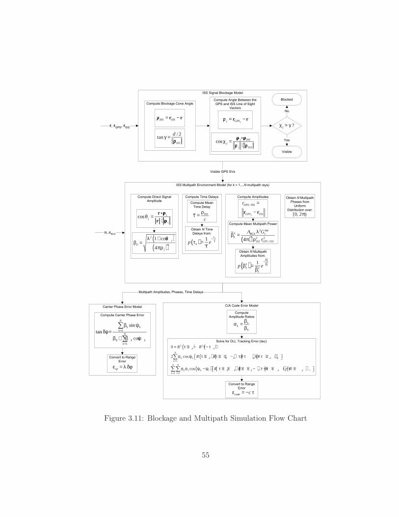
[0, 2 )π

$%

/

j

GPS ISS

GPS ISS

r =

−r r

$ &

( )2

23 2 2

/4

mpRCS r

k

ISS GPS ISS

A G

r

λβ =π ρ

%#

( )2

222

1 k

kk

k

p eβ−ββ =

β

$"'(

%

cos jj

j

θ =⋅

r

r

( )( )

2

0 2

1 cos

4

j

j

λ + θβ =

πρ

$)"

$

)"

ISS

c

ρτ =

)

" #

( ) 1 k

kp eτ−ττ =

τ

* *

( +', (

j ?χ > γ

*

+',

-

.

$+', ($%(

ISS ISS= − r r

/ 2tan

ISS

dγ =

$%(+&

/(

*'

jj GPS= − r r

cos j ISSj

j ISS

χ =⋅

0$

$

$0 (

cpε = λ δφ

$$

1

1

sintan

cos

N

k kk

N

k kk

=

0=

β ψδφ =

β + β ψ

% )"

$1%$

$

%0

0

kk

βα =β

"//) ',( #

( ) ( )

( ) ( ) ( ) ( )

( ) ( ) ( ) ( ) ( )

2 2

1

1 1

0

2 cos

cos

d d

N

k k d d k d d kk

N N

k l k l d k d l d k d lk l

R R

R R R R

R R R R

=

= =

= τ + τ − τ − τ +

α ψ τ + τ τ + τ + τ − τ − τ τ − τ + τ +

α α ψ − ψ τ + τ + τ τ + τ + τ − τ − τ + τ τ − τ + τ

$0 (

code cε = − τ

Figure 3.11: Blockage and Multipath Simulation Flow Chart

55

Chapter 4

Inertial Navigation

4.1 Fundamentals of Inertial Navigation

An INS processes measurements from sensors that sense specific forces

and inertial angular velocity. A specific force is the force per unit mass of

any non-gravitational force. A correctly initialized INS is able to determine

position and velocity without the use of external sensors or measurements. An

INS performs the following functions: [6]

• Instruments a reference frame.

• Measures specific forces.

• Models the gravitational field.

• Integrates the specific force data to obtain position and velocity.

The fundamental equation of inertial navigation comes directly from

Newton’s Second Law:

d2r

dt2= CI

BfB + g (4.1)

where r is the inertial position vector, CIB is the transformation from the INS

body frame to the inertial reference frame, fB is the total specific force vector

56

measured in the body frame, and g is the acceleration due to gravity. This

equation is integrated once to obtain velocity and a second time to obtain

position, both relative to the inertial reference frame. Accelerometers measure

the specific forces. Gyroscopes (gyros) measure the angular motion of the INS

body with respect to inertial space in order to compute CIB. An INS uses an

internal gravity model to estimate the acceleration due to gravity based on its

current estimate of position.

Inertial navigation systems can be classified into two categories: stable

platform or strapdown. Stable platform systems attempt to keep the physical

platform containing the accelerometers and gyros in a fixed orientation with

respect to the navigation frame.

In a strapdown system, the sensors are attached to the case of the INS

and remain fixed with respect to the body of the vehicle. The INS computer

uses the gyro measurements to keep track of the body’s attitude relative to

the navigation frame.

Sensors other than gyros could be used to provide attitude informa-

tion, however, an INS, by definition, uses gyroscopes because they are inertial

sensors that do not require external input.

Before the early 1980’s, gyroscopes could not measure high angular

rates and computers could not perform the strapdown computations fast enough

for strapdown systems to be practical. However, by the late 1980’s, strapdown

systems became prevalent and stable platform systems are much less common

57

today. Therefore, stable platform systems will not be discussed any further

and a strapdown system will be assumed.

4.2 INS Error Sources

The major sources of error in an INS include initialization errors, sys-

tem alignment errors, sensor errors, gravity model errors, quantization, and

computational errors.

4.2.1 Initialization Errors

An INS integrates sensed accelerations to propagate initial estimates of

position and velocity. Imperfections in the initial estimates will cause position

and velocity errors.

4.2.2 System Alignment Errors

In order to properly resolve the components of sensed acceleration in

the navigation frame, an INS must have knowledge of the orientation of the

accelerometers with respect to the navigation frame. Typically an INS will

perform an alignment process to determine the initial orientation. Errors in

the initial alignment will cause position and velocity errors.

4.2.3 Sensor Errors

Despite sensor calibration, it is not uncommon for sensor characteris-

tics to change over time and between turn-ons. These changes cannot all be

58

compensated for and result in position and velocity errors. Sources of gyro

and accelerometer errors include input axis misalignments, scale factor errors,

non-linearities, bias instability from turn-on to turn-on and bias drift after

turn-on.

4.2.3.1 Gyro Measurement Noise

Gyro measurement noise is caused by random errors in the angular

velocity measurement. This is usually the predominant error source in ring

laser and fiber optic gyros but is usually not included in error models for most

mechanical gyros. This error is modelled as zero-mean, white Gaussian noise

and causes angular random walk.

4.2.3.2 Gyro Drift (Bias)

There are two components in gyro drift. There is the gyro drift that

varies from turn-on to turn-on (also referred to as bias repeatability or bias

stability). This is modelled as a Gaussian random constant. The second part is

bias drift or variability after turn-on (sometimes referred to as in-run stability)

and is usually modelled as a random walk or first-order Markov process.

4.2.3.3 Gyro Scale Factor

Gyro scale factor error is an error in the calibrated scale factor of the

gyro. This is modelled as a Gaussian random constant for each axis.

59

4.2.3.4 Gyro Misalignments

Gyro misalignments are errors in the alignment of the gyro input (or

sensitive) axes from the orthogonal platform axes. This is modelled as a pair

of Gaussian random constants for each gyro.

4.2.3.5 Gyro G-Sensitivity

Mechanical gyros may exhibit drifts that are linear and quadratic func-

tions of acceleration. These drifts are usually not associated with ring laser or

fiber optic gyros and are modelled as Gaussian random constants.

4.2.3.6 Accelerometer Measurement Noise

Accelerometer measurement noise is caused by random errors in the

specific force measurement. This is modelled as white Gaussian noise and

causes velocity random walk.

4.2.3.7 Accelerometer Bias

There are two components in accelerometer bias error. There is the bias

repeatability that varies from turn-on to turn-on (also sometimes referred to

as bias stability). This is modelled as a random constant. The second part is

bias drift or variability after turn-on (sometimes referred to as in-run stability)

and is usually modelled as a random walk or first-order Markov process.

60

4.2.3.8 Accelerometer Scale Factor

Accelerometer scale factor error is an error in the calibrated scale factor

of the accelerometer. This is modelled as a Gaussian random constant for each

axis.

4.2.3.9 Accelerometer Misalignments

Accelerometer misalignments are errors in the alignment of the ac-

celerometer input (or sensitive) axes from the orthogonal platform axes. This

is modelled as a pair of Gaussian random constants for each accelerometer.

4.2.3.10 Accelerometer Non-linearity

Accelerometers may exhibit errors that are quadratic functions of ac-

celeration. This error source is modelled by six Gaussian random constants

for each axis.

4.2.4 Gravity Model Errors

The Earth’s gravity field cannot be modelled perfectly and so an INS

designer must choose a gravity field model that meets the accuracy require-

ments of the particular application.

4.2.5 Quantization and Computational Errors

The navigation equations are typically performed by a digital computer

where quantization, overflow and numeric errors can occur.

61

4.3 INS Error Model

The INS error model has a number of uses. During INS testing, optimal

estimation theory can be applied to process all of the available test data to

obtain the best possible estimates of the sources of error of the INS under

test. In an integrated GPS/INS, an error state space (indirect) Kalman filter

uses the INS error model in the propagation step to predict the errors at the

next measurement time. The INS error model is also used in the design of

the GPS/INS Kalman filter to determine which error sources are important to

include in the filter and which ones can be ignored.

The navigation errors committed by an inertial navigation system can

be modelled by a set of first order, linear ordinary differential equations. These

equations are derived using linear perturbation theory and allow the use of

optimal estimation theory to estimate and remove the errors.

4.3.1 Derivation of INS Error Model

The derivation of the error model for a strapdown INS using quater-

nions presented in this section is based on Friedland [16] and provides some of

the missing steps. The first step in deriving the INS error model is to define

the state vector x as:

x =

rvq

(4.2)

where r is the position vector, v is the velocity vector and q is the quaternion

representing the body to inertial reference frame transformation. The system

62

will be driven by the angular velocity sensed by the gyros and specific forces

sensed by the accelerometers, so the forcing function vector u is defined as

follows:

u =

[ωf

](4.3)

Using these definitions and equations (4.1) and (5.77), the fundamental

equations of inertial navigation can be expressed in first order form as:

x =

rvq

=

v (t)CI

B (q) f (t) + g (r)Ω (ω) q (t)

= Γ (x, u, t) (4.4)

Let δx represent the error in the INS-indicated position, velocity and

attitude such that:

xtrue = x + δx (4.5)

where x is the INS-indicated state. Taking the time derivative of this equation

and rearranging leads to:

δx = xtrue − ˙x (4.6)

Also, let δu represent the error in the measured angular velocity and specific

force vector such that:

utrue = u + δu (4.7)

Expanding equation (4.4) in a Taylor’s series about the INS-indicated

state results in:

xtrue = Γ (xtrue, t) = Γ (x, t) +[

∂Γ(x,u,t)∂x

]∗(xtrue − x)

+[

∂Γ(x,u,t)∂u

]∗(utrue − u) + · · ·

(4.8)

63

where []∗ indicates that the partial derivative is evaluated on the INS-indicated

solution. If second order and higher terms are neglected and the proper substi-

tutions from equations (4.5), (4.6), and (4.7) are made, the following equation

is obtained:

δx (t) =

[∂Γ (x, u, t)

∂x

]∗δx (t) +

[∂Γ (x, u, t)

∂u

]∗δu (t) (4.9)

Taking the indicated partial derivatives leads to the following set of

first order, linear ordinary differential equations for INS errors:

δrδvδq

=

03×3 I3×3 03×4

∂g(r)∂r

03×3∂CI

B

∂qf (t)

04×3 04×3 Ω (ω)

δrδvδq

+

03×3 03×3

03×3 CIB (q)

∂Ω∂ω

q 03×3

[δωδf

]

(4.10)

In order to simplify the expression∂CI

B

∂qδq f (t), it is convenient to define a

matrix D such that∂CI

B

∂qδq f (t) ≡ D

(q, f

)δq where:

DT = 2

q1f1 + q2f2 + q3f3 q2f1 − q1f2 − q4f3 q3f1 + q4f2 − q1f3

−q2f1 + q1f2 + q4f3 q1f1 + q2f2 + q3f3 −q4f1 + q3f2 − q2f3

−q3f1 − q4f2 + q1f3 q4f1 − q3f2 + q2f3 q1f1 + q2f2 + q3f3

q4f1 − q3f2 + q2f3 q3f1 + q4f2 − q1f3 −q2f1 + q1f2 + q4f3

(4.11)

With this definition and noting that ∂Ω∂ω

q = Q, where Q is defined in Section

2.1.7, (4.10) simplifies to:

δrδvδq

=

03×3 I3×3 03×4

∂g(r)∂r

03×3 D(q, f

)

04×3 04×3 Ω (ω)

δrδvδq

+

03×3 03×3

03×3 CIB (q)

Q (q) 03×3

[δωδf

]

(4.12)

64

where the gravity gradient matrix, ∂g(r)∂r

for a two-body gravity field is:

∂g

∂r=

3µx2

r5 − µr3

3µxyr5

3µxzr5

3µxyr5

3µy2

r5 − µr3

3µyzr5

3µxzr5

3µyzr5

3µz2

r5 − µr3

(4.13)

4.3.2 Sensor Error Models

The error models for gyros and accelerometers are described in this

section. The models described in this section serve two purposes. First, they

form the basis for the truth model needed for covariance analysis. Second,

when an error source is determined to have a significant effect on navigation

error, the variables associated with that error source can be added to the error

state vector and estimated by the GPS/INS Kalman filter. Since gyros and

accelerometers are subject to random errors, stochastic models are needed to

adequately characterize them.

4.3.2.1 Gyro Error Model

The purpose of the gyro error model is to provide the δω term in (4.12).

The specific details of any gyro error model depend on the type of gyro and

the characteristics of the errors found during testing. Gyro manufacturers

usually provide some specification numbers but do not publish the detailed

error models. Therefore, early in the navigation system design process, before

a particular gyro has been selected, simplified error models are used to perform

trade studies and requirements analysis.

The error model for a set of three orthogonal gyros can be defined

65

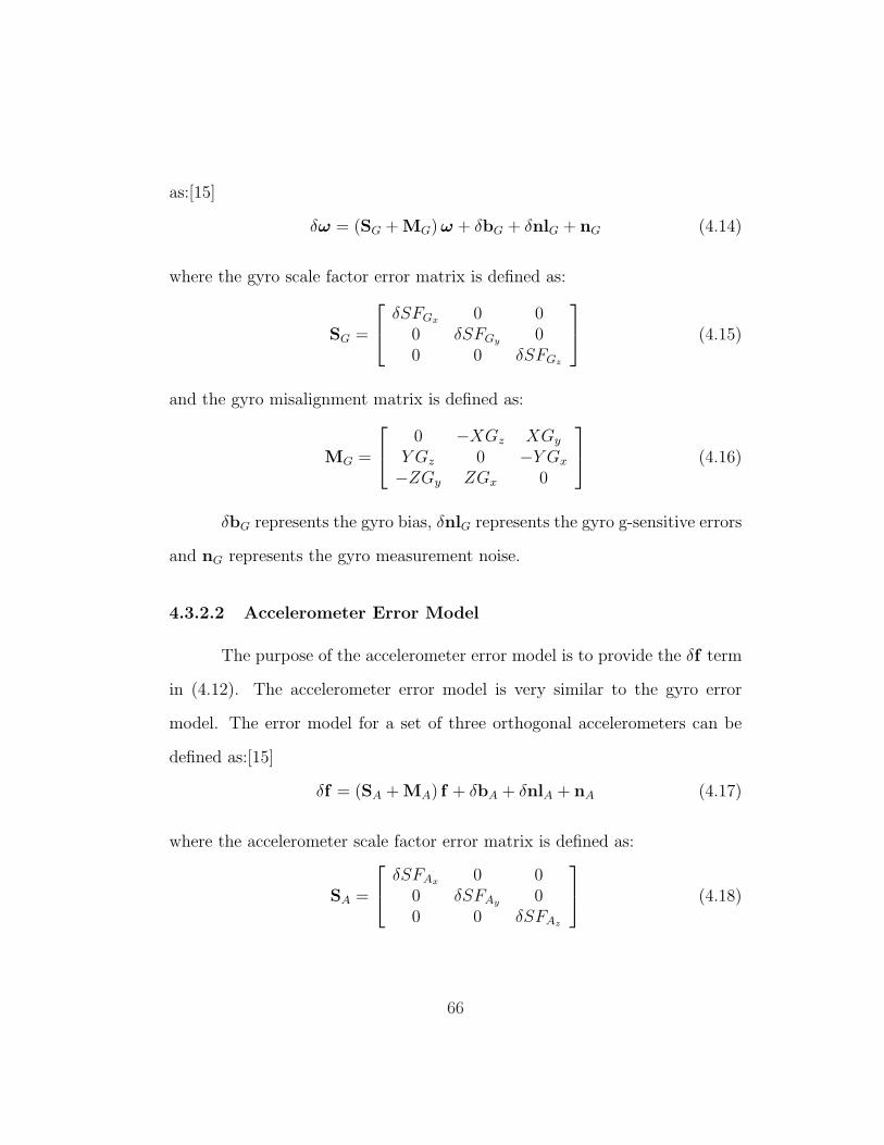
as:[15]

δω = (SG + MG) ω + δbG + δnlG + nG (4.14)

where the gyro scale factor error matrix is defined as:

SG =

δSFGx 0 00 δSFGy 00 0 δSFGz

(4.15)

and the gyro misalignment matrix is defined as:

MG =

0 −XGz XGy

Y Gz 0 −Y Gx

−ZGy ZGx 0

(4.16)

δbG represents the gyro bias, δnlG represents the gyro g-sensitive errors

and nG represents the gyro measurement noise.

4.3.2.2 Accelerometer Error Model

The purpose of the accelerometer error model is to provide the δf term

in (4.12). The accelerometer error model is very similar to the gyro error

model. The error model for a set of three orthogonal accelerometers can be

defined as:[15]

δf = (SA + MA) f + δbA + δnlA + nA (4.17)

where the accelerometer scale factor error matrix is defined as:

SA =

δSFAx 0 00 δSFAy 00 0 δSFAz

(4.18)

66

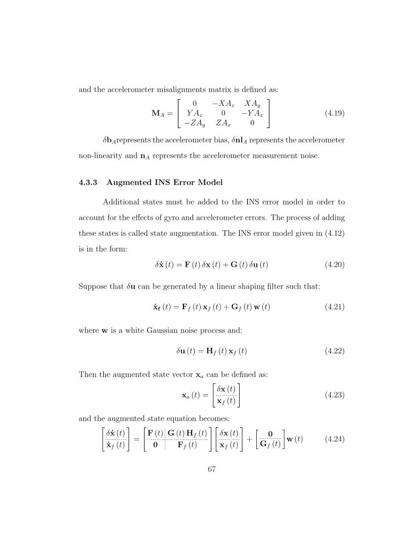
and the accelerometer misalignments matrix is defined as:

MA =

0 −XAz XAy

Y Az 0 −Y Ax

−ZAy ZAx 0

(4.19)

δbArepresents the accelerometer bias, δnlA represents the accelerometer

non-linearity and nA represents the accelerometer measurement noise.

4.3.3 Augmented INS Error Model

Additional states must be added to the INS error model in order to

account for the effects of gyro and accelerometer errors. The process of adding

these states is called state augmentation. The INS error model given in (4.12)

is in the form:

δx (t) = F (t) δx (t) + G (t) δu (t) (4.20)

Suppose that δu can be generated by a linear shaping filter such that:

xf (t) = Ff (t)xf (t) + Gf (t)w (t) (4.21)

where w is a white Gaussian noise process and:

δu (t) = Hf (t)xf (t) (4.22)

Then the augmented state vector xa can be defined as:

xa (t) =

[δx (t)

xf (t)

](4.23)

and the augmented state equation becomes:[δx (t)

xf (t)

]=

[F (t) G (t)Hf (t)

0 Ff (t)

][δx (t)

xf (t)

]+

[0

Gf (t)

]w (t) (4.24)

67

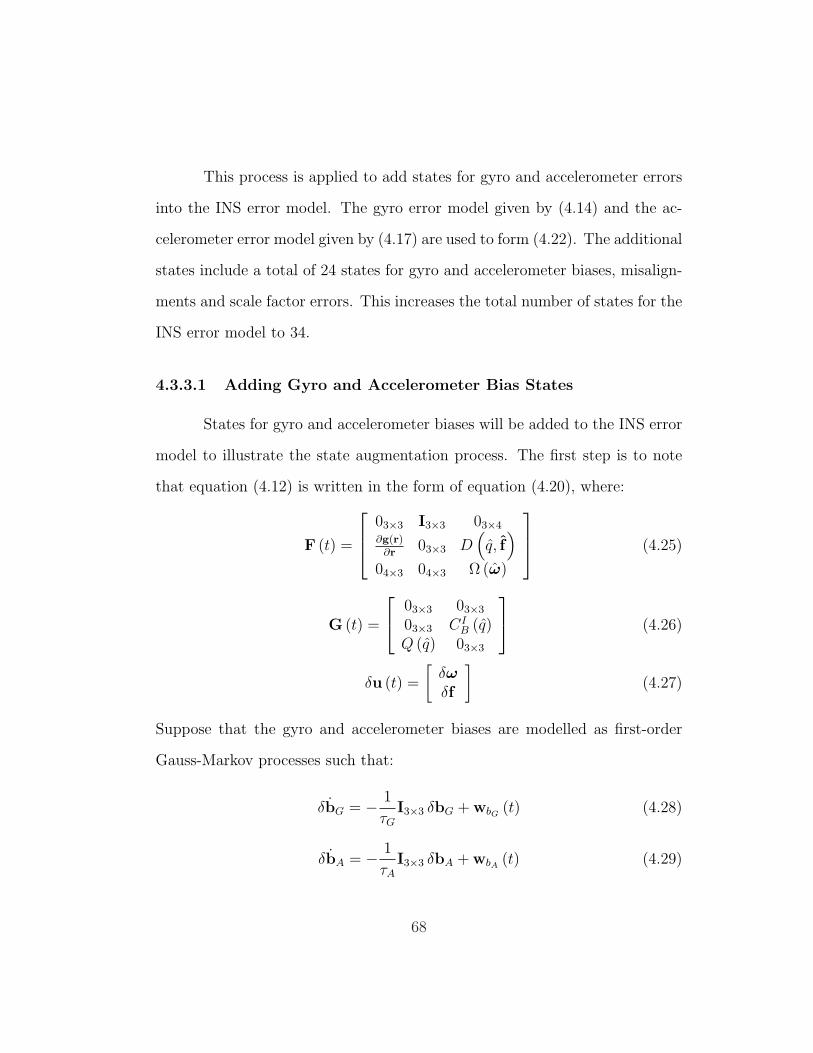
This process is applied to add states for gyro and accelerometer errors

into the INS error model. The gyro error model given by (4.14) and the ac-

celerometer error model given by (4.17) are used to form (4.22). The additional

states include a total of 24 states for gyro and accelerometer biases, misalign-

ments and scale factor errors. This increases the total number of states for the

INS error model to 34.

4.3.3.1 Adding Gyro and Accelerometer Bias States

States for gyro and accelerometer biases will be added to the INS error

model to illustrate the state augmentation process. The first step is to note

that equation (4.12) is written in the form of equation (4.20), where:

F (t) =

03×3 I3×3 03×4

∂g(r)∂r

03×3 D(q, f

)

04×3 04×3 Ω (ω)

(4.25)

G (t) =

03×3 03×3

03×3 CIB (q)

Q (q) 03×3

(4.26)

δu (t) =

[δωδf

](4.27)

Suppose that the gyro and accelerometer biases are modelled as first-order

Gauss-Markov processes such that:

δbG = − 1

τG

I3×3 δbG + wbG(t) (4.28)

δbA = − 1

τA

I3×3 δbA + wbA(t) (4.29)

68

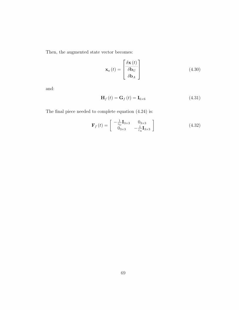
Then, the augmented state vector becomes:

xa (t) =

δx (t)

δbG

δbA

(4.30)

and:

Hf (t) = Gf (t) = I6×6 (4.31)

The final piece needed to complete equation (4.24) is:

Ff (t) =

[ − 1τG

I3×3 03×3

03×3 − 1τA

I3×3

](4.32)

69

Chapter 5

GPS/INS Integration and Simulation

The integration of GPS and INS is achieved using a Kalman filter.

This chapter describes the integration architecture, Kalman filter design and

the GPS/INS simulation.

5.1 GPS/INS Simulation Description

The processes used to generate the chaser and ISS true trajectories,

the accelerometer and gyro measurements, and the GPS measurements for

the GPS/INS simulation are described in this section.

5.1.1 Rendezvous Trajectory Generation

The GPS/INS simulation is driven by the true trajectories of the chaser

and ISS. In order to generate the true trajectories, the following equations of

motion are integrated using an eighth-order Runge-Kutta numerical integrator

with a fixed step size of 0.5 seconds:

d2r

dt2= fdrag + fthrust + g (5.1)

70

where the acceleration due to atmospheric drag, fdrag, is computed using:

fdrag = −1

2

CDA

mρV 2

rel

Vrel

‖Vrel‖ (5.2)

where CD is the drag coefficient, A is the reference surface area, m is the mass.

The atmospheric density, ρ, is computed using the Harris-Priester density

model, which is described in Montenbruck [30].

Thrust is applied to maneuver the chaser spacecraft towards the ISS.

The magnitude of the acceleration due to thrust is assumed to be constant

during a maneuver and the direction of the thrust acceleration is assumed to

be fixed in the body frame. The process used to calculate the thrust direction

and duration is described in the next section.

The acceleration due to gravity, g, resulting from a spherical harmonic

gravity field is given by the gradient of the geopotential function:

g = ∇U (5.3)

where the geopotential function is given by:

U =µ

r

N∑n=2

n∑m=0

(RE

r

)n

Pnm sin φ [Cnm cos(mλ) + Snm sin(mλ)] (5.4)

71

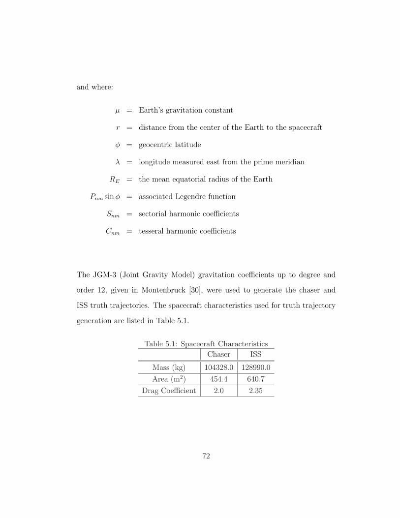
and where:

µ = Earth’s gravitation constant

r = distance from the center of the Earth to the spacecraft

φ = geocentric latitude

λ = longitude measured east from the prime meridian

RE = the mean equatorial radius of the Earth

Pnm sin φ = associated Legendre function

Snm = sectorial harmonic coefficients

Cnm = tesseral harmonic coefficients

The JGM-3 (Joint Gravity Model) gravitation coefficients up to degree and

order 12, given in Montenbruck [30], were used to generate the chaser and

ISS truth trajectories. The spacecraft characteristics used for truth trajectory

generation are listed in Table 5.1.

Table 5.1: Spacecraft Characteristics

Chaser ISS

Mass (kg) 104328.0 128990.0

Area (m2) 454.4 640.7

Drag Coefficient 2.0 2.35

72

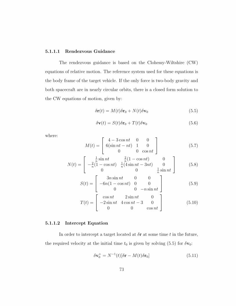
5.1.1.1 Rendezvous Guidance

The rendezvous guidance is based on the Clohessy-Wiltshire (CW)

equations of relative motion. The reference system used for these equations is

the body frame of the target vehicle. If the only force is two-body gravity and

both spacecraft are in nearly circular orbits, there is a closed form solution to

the CW equations of motion, given by:

δr(t) = M(t)δr0 + N(t)δv0 (5.5)

δv(t) = S(t)δr0 + T (t)δv0 (5.6)

where:

M(t) =

4− 3 cos nt 0 06(sin nt− nt) 1 0

0 0 cos nt

(5.7)

N(t) =

1n

sin nt 2n(1− cos nt) 0

− 2n(1− cos nt) 1

n(4 sin nt− 3nt) 0

0 0 1n

sin nt

(5.8)

S(t) =

3n sin nt 0 0−6n(1− cos nt) 0 0

0 0 −n sin nt

(5.9)

T (t) =

cos nt 2 sin nt 0−2 sin nt 4 cos nt− 3 0

0 0 cos nt

(5.10)

5.1.1.2 Intercept Equation

In order to intercept a target located at δr at some time t in the future,

the required velocity at the initial time t0 is given by solving (5.5) for δv0:

δv+0 = N−1(t)[δr−M(t)δr0] (5.11)

73

The required change in velocity needed to intercept the target is:

∆v0 = δv+0 − δv−0 (5.12)

where δv−0 is the relative velocity before the maneuver.

5.1.1.3 Glideslope Targeting

The glideslope targeting algorithm is described in Hablani [20] and

summarized here. At the initial time, the chaser vehicle is located at δr0 with

relative velocity equal to δv−0 . It is required to arrive at δr = δrT in a transfer

time of T .

A straight line from δr0 to δrT , which is the commanded path, is de-

noted by the vector ρ. The boundary conditions of ρ are ρ(t0) = δr0 − δrT

and ρ(T ) = 0.

The direction of the straight path is given by the unit vector uρ:

uρ =

x0−xT

ρ0y0−yT

ρ0z0−zT

ρ0

(5.13)

therefore, ρ(t) = ρuρ.

The glideslope guidance specifies the distance to go, ρ, as a function

of time so that the chaser is commanded to reach δrT in a period T with an

arrival velocity of ρTuρ, where ρT is a safe relative speed at the distance δrT

from the target.

74

As ρ diminishes, ρ must also diminish. The following linear relationship

is postulated:

ρ(t) = aρ(t) + ρT (5.14)

The boundary conditions on ρ and ρ at t0 are:

ρ(t0) = ρ0

ρ(t0) = ρ0 < 0 (5.15)

and at t = T :

ρ(T ) = 0

ρ(T ) = ρT < 0 (5.16)

The initial distance to go, ρ0, the initial commanded velocity, ρ0 and the final

commanded arrival velocity, ρT , are all known or specified. The slope, a is

given by:

a =ρ0 − ρT

ρ0

< 0 (5.17)

The solution to (5.14) with boundary conditions given by (5.15) and (5.16) is:

ρ(t) = ρ0eat +

ρT

a[eat − 1] (5.18)

and the transfer time is given by:

T =1

aln

ρT

ρ0

(5.19)

75

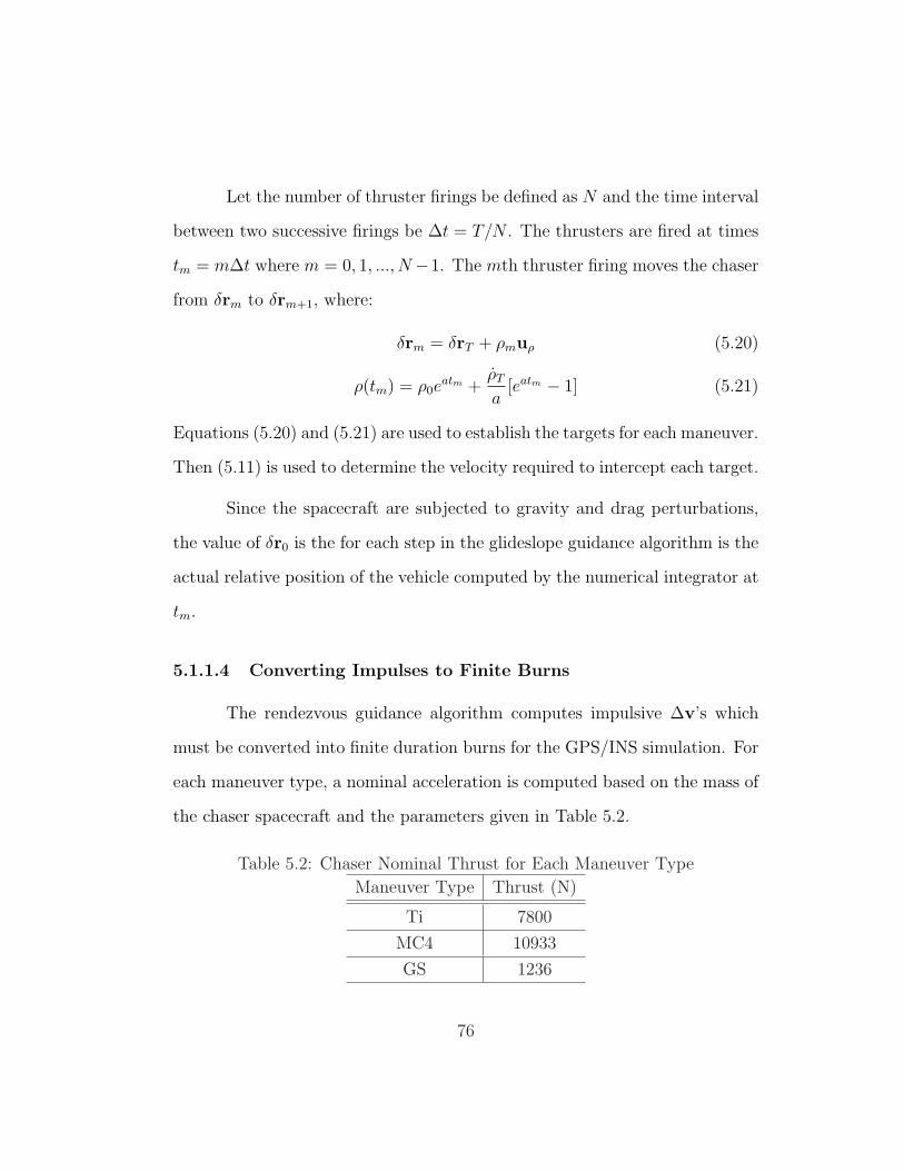
Let the number of thruster firings be defined as N and the time interval

between two successive firings be ∆t = T/N . The thrusters are fired at times

tm = m∆t where m = 0, 1, ..., N−1. The mth thruster firing moves the chaser

from δrm to δrm+1, where:

δrm = δrT + ρmuρ (5.20)

ρ(tm) = ρ0eatm +

ρT

a[eatm − 1] (5.21)

Equations (5.20) and (5.21) are used to establish the targets for each maneuver.

Then (5.11) is used to determine the velocity required to intercept each target.

Since the spacecraft are subjected to gravity and drag perturbations,

the value of δr0 is the for each step in the glideslope guidance algorithm is the

actual relative position of the vehicle computed by the numerical integrator at

tm.

5.1.1.4 Converting Impulses to Finite Burns

The rendezvous guidance algorithm computes impulsive ∆v’s which

must be converted into finite duration burns for the GPS/INS simulation. For

each maneuver type, a nominal acceleration is computed based on the mass of

the chaser spacecraft and the parameters given in Table 5.2.

Table 5.2: Chaser Nominal Thrust for Each Maneuver Type

Maneuver Type Thrust (N)

Ti 7800

MC4 10933

GS 1236

76

The magnitude of the thrust acceleration is given by:

athrust =thrust

mass(5.22)

The burn duration is computed by:

tburn =‖∆v‖athrust

(5.23)

Then the burn duration, tburn, is rounded up to the next even number of

seconds in order to start and stop the burns on integer seconds in simulation

time. The burn start time and stop times are computed by:

tstart = tm − tburn

2

tstop = tm +tburn

2

The thrust acceleration is then lowered to obtain the desired burn du-

ration. The direction of the thrust acceleration vector is held fixed in the

spacecraft body frame and is given by:

uthrust =∆v

‖∆v‖ (5.24)

5.1.1.5 Open Loop vs. Closed Loop Guidance

The true trajectory for the simulations in this dissertation are com-

puted and stored in a file before the measurement generation process is run.

Therefore, the output of the navigation process cannot be used to change

the true trajectory. So the guidance scheme used to generate the rendezvous

trajectories is not considered to be closed-loop.

77

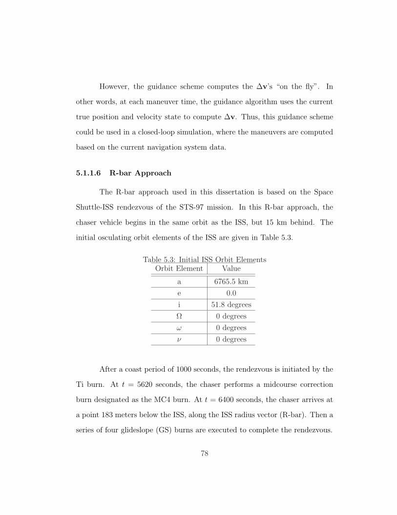
However, the guidance scheme computes the ∆v’s “on the fly”. In

other words, at each maneuver time, the guidance algorithm uses the current

true position and velocity state to compute ∆v. Thus, this guidance scheme

could be used in a closed-loop simulation, where the maneuvers are computed

based on the current navigation system data.

5.1.1.6 R-bar Approach

The R-bar approach used in this dissertation is based on the Space

Shuttle-ISS rendezvous of the STS-97 mission. In this R-bar approach, the

chaser vehicle begins in the same orbit as the ISS, but 15 km behind. The

initial osculating orbit elements of the ISS are given in Table 5.3.

Table 5.3: Initial ISS Orbit ElementsOrbit Element Value

a 6765.5 km

e 0.0

i 51.8 degrees

Ω 0 degrees

ω 0 degrees

ν 0 degrees

After a coast period of 1000 seconds, the rendezvous is initiated by the

Ti burn. At t = 5620 seconds, the chaser performs a midcourse correction

burn designated as the MC4 burn. At t = 6400 seconds, the chaser arrives at

a point 183 meters below the ISS, along the ISS radius vector (R-bar). Then a

series of four glideslope (GS) burns are executed to complete the rendezvous.

78

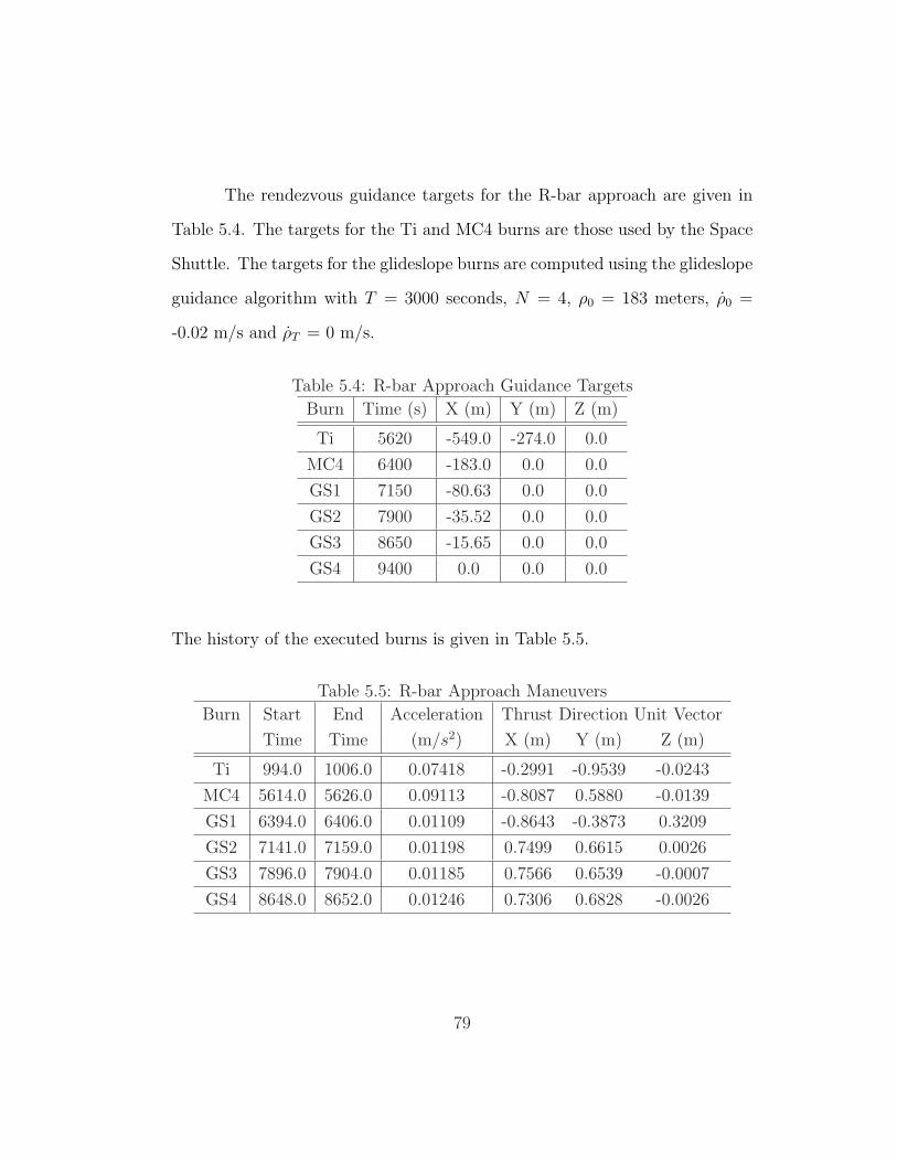
The rendezvous guidance targets for the R-bar approach are given in

Table 5.4. The targets for the Ti and MC4 burns are those used by the Space

Shuttle. The targets for the glideslope burns are computed using the glideslope

guidance algorithm with T = 3000 seconds, N = 4, ρ0 = 183 meters, ρ0 =

-0.02 m/s and ρT = 0 m/s.

Table 5.4: R-bar Approach Guidance Targets

Burn Time (s) X (m) Y (m) Z (m)

Ti 5620 -549.0 -274.0 0.0

MC4 6400 -183.0 0.0 0.0

GS1 7150 -80.63 0.0 0.0

GS2 7900 -35.52 0.0 0.0

GS3 8650 -15.65 0.0 0.0

GS4 9400 0.0 0.0 0.0

The history of the executed burns is given in Table 5.5.

Table 5.5: R-bar Approach Maneuvers

Burn Start End Acceleration Thrust Direction Unit Vector

Time Time (m/s2) X (m) Y (m) Z (m)

Ti 994.0 1006.0 0.07418 -0.2991 -0.9539 -0.0243

MC4 5614.0 5626.0 0.09113 -0.8087 0.5880 -0.0139

GS1 6394.0 6406.0 0.01109 -0.8643 -0.3873 0.3209

GS2 7141.0 7159.0 0.01198 0.7499 0.6615 0.0026

GS3 7896.0 7904.0 0.01185 0.7566 0.6539 -0.0007

GS4 8648.0 8652.0 0.01246 0.7306 0.6828 -0.0026

79

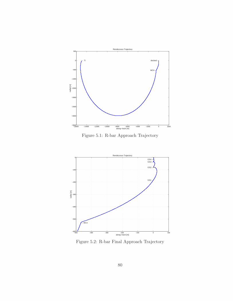
−16000 −14000 −12000 −10000 −8000 −6000 −4000 −2000 0 2000−3500

−3000

−2500

−2000

−1500

−1000

−500

0

500

along−track [m]

radi

al [m

]

← Ti docked→

MC4→

Rendezvous Trajectory

Figure 5.1: R-bar Approach Trajectory

−500 −400 −300 −200 −100 0 100−600

−500

−400

−300

−200

−100

0

along−track [m]

radi

al [m

]

← MC4

GS1→

GS2→

GS3→GS4→


Figure 5.2: R-bar Final Approach Trajectory

80

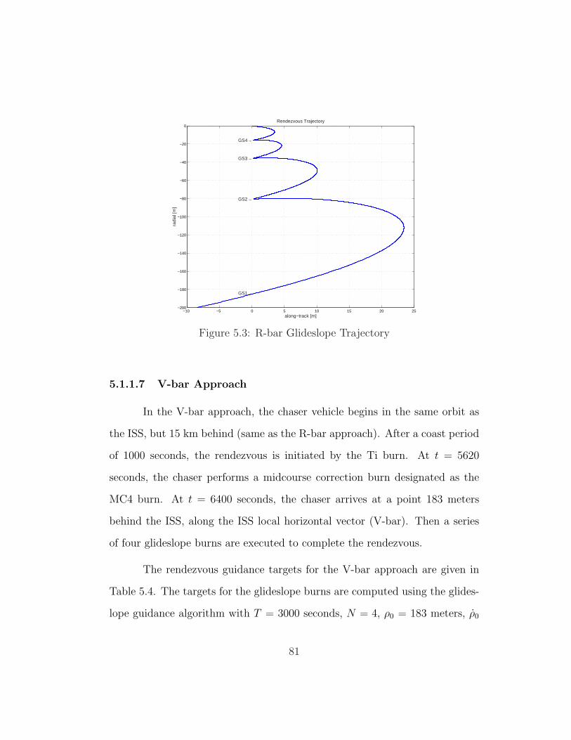
−10 −5 0 5 10 15 20 25−200

−180

−160

−140

−120

−100

−80

−60

−40

−20

0

along−track [m]

radi

al [m

]

GS1→

GS2→

GS3→

GS4→


Figure 5.3: R-bar Glideslope Trajectory

5.1.1.7 V-bar Approach

In the V-bar approach, the chaser vehicle begins in the same orbit as

the ISS, but 15 km behind (same as the R-bar approach). After a coast period

of 1000 seconds, the rendezvous is initiated by the Ti burn. At t = 5620

seconds, the chaser performs a midcourse correction burn designated as the

MC4 burn. At t = 6400 seconds, the chaser arrives at a point 183 meters

behind the ISS, along the ISS local horizontal vector (V-bar). Then a series

of four glideslope burns are executed to complete the rendezvous.

The rendezvous guidance targets for the V-bar approach are given in

Table 5.4. The targets for the glideslope burns are computed using the glides-

lope guidance algorithm with T = 3000 seconds, N = 4, ρ0 = 183 meters, ρ0

81

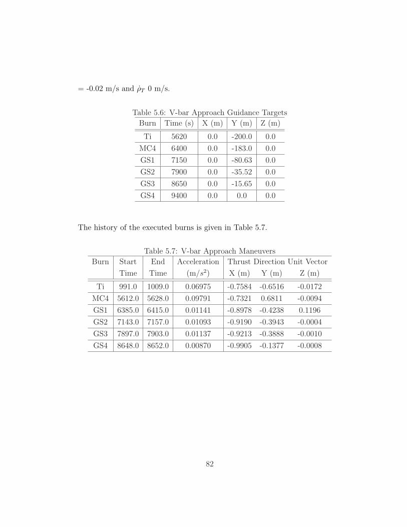
= -0.02 m/s and ρT 0 m/s.

Table 5.6: V-bar Approach Guidance Targets

Burn Time (s) X (m) Y (m) Z (m)

Ti 5620 0.0 -200.0 0.0

MC4 6400 0.0 -183.0 0.0

GS1 7150 0.0 -80.63 0.0

GS2 7900 0.0 -35.52 0.0

GS3 8650 0.0 -15.65 0.0

GS4 9400 0.0 0.0 0.0

The history of the executed burns is given in Table 5.7.

Table 5.7: V-bar Approach Maneuvers

Burn Start End Acceleration Thrust Direction Unit Vector

Time Time (m/s2) X (m) Y (m) Z (m)

Ti 991.0 1009.0 0.06975 -0.7584 -0.6516 -0.0172

MC4 5612.0 5628.0 0.09791 -0.7321 0.6811 -0.0094

GS1 6385.0 6415.0 0.01141 -0.8978 -0.4238 0.1196

GS2 7143.0 7157.0 0.01093 -0.9190 -0.3943 -0.0004

GS3 7897.0 7903.0 0.01137 -0.9213 -0.3888 -0.0010

GS4 8648.0 8652.0 0.00870 -0.9905 -0.1377 -0.0008

82

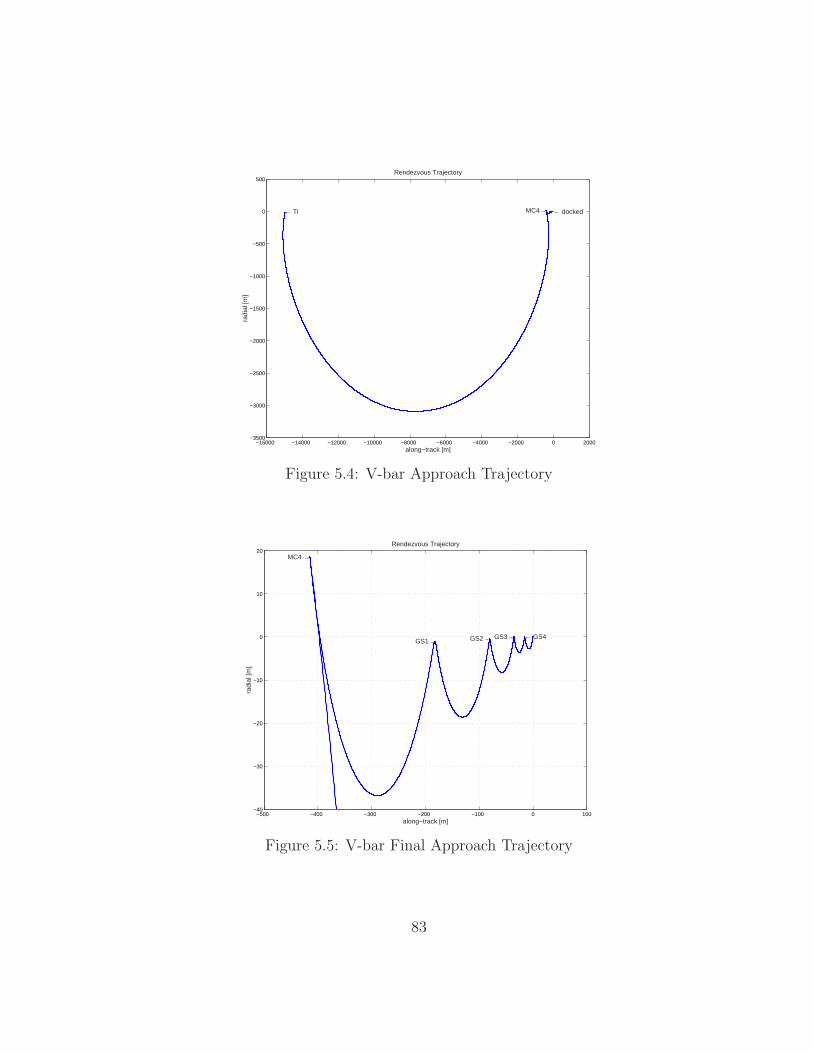
−16000 −14000 −12000 −10000 −8000 −6000 −4000 −2000 0 2000−3500

−3000

−2500

−2000

−1500

−1000

−500

0

500

along−track [m]

radi

al [m

]

← Ti ← dockedMC4→


Figure 5.4: V-bar Approach Trajectory

−500 −400 −300 −200 −100 0 100−40

−30

−20

−10

0

10

20

along−track [m]

radi

al [m

]

MC4 →

GS1→ GS2→ GS3→ ← GS4


Figure 5.5: V-bar Final Approach Trajectory

83

5.1.2 Generation of Simulated INS Measurements

The process used to generate simulated INS measurements is described

in this section. In modern digital systems, gyro and accelerometer outputs

are provided in the form of velocity and angle increments. The torques and

specific forces are summed over a short time interval, δt, referred to as the

sampling interval. This corresponds to the raw data rate of the IMU or some

multiple of it. The accumulated angle and velocity contains the high frequency

information of the dynamics even if δt is comparatively long. Typical values

for δt are 0.005 to 0.02 seconds for highly dynamic applications. For a space

application, the samples times can be much longer as shown in Section 5.2.2.1.

Let ∆θl be defined as a vector containing the angular increments from

all three gyros summed over the lth time increment, where the sampling in-

tervals, δt = tl − tl−1, are constant. The data received from the gyros can be

expressed as:

∆θl =

∫ tl

tl−1

ωBI (t) dt (5.25)

Similarly, let ∆vl be defined as a vector containing the velocity incre-

ments from all three accelerometers summed over the lth time increment. The

data received from the accelerometers can be expressed as:

∆vl =

∫ tl

tl−1

f (t) dt (5.26)

The gyro and accelerometer measurements can be represented by (5.25)

and (5.26) respectively. These equations can also be expressed as differential

84

equations over the sampling interval:

∆θl = ωBI (5.27)

∆vl = fB (5.28)

The measured quantities are equal to the true quantities minus the errors,

therefore:

∆θl = ωBItrue − δω (5.29)

∆vl = fBtrue − δf (5.30)

Substituting from the gyro and accelerometer error models, neglecting the

non-linearity terms, leads to the following:

∆θl = (I− SG −MG)3×3 ωBItrue − δbG − nG (5.31)

∆vl = (I− SA −MA)3×3 fBtrue − δbA − nA (5.32)

Since the scale factor and misalignment errors are modelled as random

constants, the first terms of these equations are deterministic after turn-on.

The gyro and accelerometer biases are modelled as first-order Gauss-Markov

processes for the SIGI sensors, therefore, the following additional equations

need to be integrated:

δbG = − 1

τG

I3×3 δbG + wbG(t) (5.33)

δbA = − 1

τA

I3×3 δbA + wbA(t) (5.34)

85

These equations can be written for the gyros and accelerometers in the follow-

ing form:

x (t) = F (t)x (t) + B (t)u (t) + G (t)w (t) (5.35)

The gyro equations can be written:

[δbG

∆θ

]=

[FbG

03×3

−I3×3 03×3

][δbG

∆θ

]+

[03×3 03×3

I− SG −MG 03×3

][03×1

ωBItrue

]

+

[I3×3 03×3

03×3 −I3×3

][wbG

nG

](5.36)

The accelerometer equations can be written:

[δbA

∆v

]=

[FbA

03×3

−I3×3 03×3

][δbA

∆v

]+

[03×3 03×3

I− SA −MA 03×3

][03×1

fBtrue

]

+

[I3×3 03×3

03×3 −I3×3

][wbA

nA

](5.37)

The contributions to the accumulated sensor measurements can be separated

into deterministic and stochastic parts. The middle terms of these equations

represent the deterministic contributions to the measurements and will be

handled separately. The stochastic equations then become:

[δbG

∆θ

]=

[FbG

03×3

−I3×3 03×3

][δbG

∆θ

]+

[I3×3 03×3

03×3 −I3×3

][wbG

nG

](5.38)

[δbA

∆v

]=

[FbA

03×3

−I3×3 03×3

][δbA

∆v

]+

[I3×3 03×3

03×3 −I3×3

][wbA

nA

](5.39)

86

The variables FbGand FbA

depend on the type of stochastic process used to

model the gyros and accelerometers. If gyro and accelerometer biases are

modelled as first order Gauss-Markov processes, then for three identical gyros

and three identical accelerometers:

FbG= − 1

τG

I3×3

FbA= − 1

τA

I3×3

where τG and τA are the gyro and accelerometer bias correlation times. For

details on stochastic process modelling, see Appendix B.

In order to generate the gyro and accelerometer measurements, these

differential equations are converted to equivalent stochastic difference equa-

tions of the following form:

x (ti+1) = Φ (ti+1, ti)x (ti) + wd (ti) (5.40)

The stochastic difference equations are then used to propagate the biases and

to accumulate the stochastic contribution to the sensor measurements. The

parameters presented in Table 5.8 were used to simulate the gyros and ac-

celerometers of the SIGI.

87

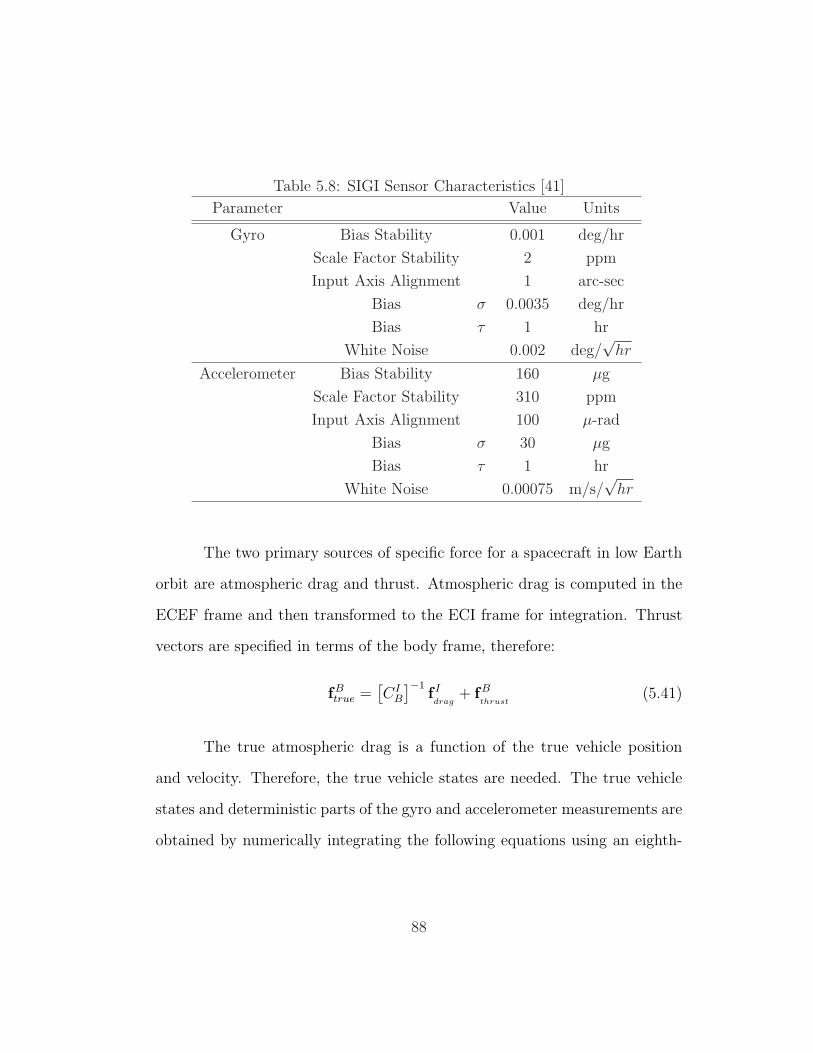
Table 5.8: SIGI Sensor Characteristics [41]

Parameter Value Units

Gyro Bias Stability 0.001 deg/hr

Scale Factor Stability 2 ppm

Input Axis Alignment 1 arc-sec

Bias σ 0.0035 deg/hr

Bias τ 1 hr

White Noise 0.002 deg/√

hr

Accelerometer Bias Stability 160 µg


Input Axis Alignment 100 µ-rad

Bias σ 30 µg

Bias τ 1 hr

White Noise 0.00075 m/s/√

hr

The two primary sources of specific force for a spacecraft in low Earth

orbit are atmospheric drag and thrust. Atmospheric drag is computed in the

ECEF frame and then transformed to the ECI frame for integration. Thrust

vectors are specified in terms of the body frame, therefore:

fBtrue =

[CI

B

]−1f I

drag+ fB

thrust(5.41)

The true atmospheric drag is a function of the true vehicle position

and velocity. Therefore, the true vehicle states are needed. The true vehicle

states and deterministic parts of the gyro and accelerometer measurements are

obtained by numerically integrating the following equations using an eighth-

88

order Runge-Kutta integrator:

rtrue

vtrue

qtrue

∆θ∆v

=

vtrue

CIBfB

true + gtrue

Ω (ωBItrue) qtrue

(I− SG −MG)ωBI

(I− SA −MA)fBtrue

(5.42)

Instead of carrying forward the ∆θ and ∆v states forward from one

integration step to the next, they are zeroed out after they are added to the

stochastic contributions and recorded at each sample time in order to simulate

the measurement accumulation process.

5.1.3 GPS Measurement Generation

This section describes the models used to generate simulated GPS mea-

surements for C/A code pseudorange and carrier phase measurements.

5.1.3.1 Pseudorange and Carrier Phase Measurements

The GPS pseudorange and carrier phase measurements are generated

at a once per second rate using the following equations:

P (t) = ρ + [c− ρ] ∆tR − c∆tS + ∆URE + ∆iono + ∆mp + εpr (5.43)

λΦ(t) = ρ + [c− ρ] ∆tR − c∆tS + ∆URE + ∆iono + ∆mp + λN + εcp

The pseudorange and carrier phase range measurement errors are as-

sumed to be zero-mean, white Gaussian random numbers with the following

89

standard deviations:

σεpr = 2.0 m (5.44)

σεcp = 0.02 m (5.45)

The multipath model is described in Chapter 3. The models used to

compute the GPS SV clock and ephemeris errors, and ionospheric delays are

described in the sections below.

5.1.3.2 Single Difference Carrier Phase Measurements

The single difference carrier phase measurements are generated for each

GPS SV as follows:

1. If the GPS SV is visible at the chaser, the carrier phase measurement

for the chaser is generated.

2. If the GPS SV is visible at the ISS, the carrier phase measurement for

the ISS is generated.

3. If the GPS SV is visible to both the chaser and ISS, the single difference

carrier phase measurement is generated by subtracting the ISS measure-

ment from the chaser measurement.

Each carrier phase measurement is generated with all appropriate error

sources included. When the single difference is formed, no assumption is made

about the cancellation of errors. Since the common errors between the chaser

90

and ISS are not exactly equal, there are small residual errors remaining in the

single difference carrier phase measurements sent to the Kalman filter.

5.1.3.3 GPS Receiver Clock Model

The GPS receiver clock model is described in Brown and Hwang [7] and

summarized in this section. Let bc denote the receiver clock bias converted to

meters, such that:

bc = c∆tR (5.46)

where c is the speed of light. The receiver clock bias and drift are modelled as

random-walk processes: [13]

bc = dc + wf + ch (5.47)

dc = wg (5.48)

where dc is the clock drift, h is the frequency correction due to relativistic

effects, and wf and wg are zero-mean white Gaussian variables with power

spectral amplitudes of Sf and Sg, respectively.

In near circular orbits, h can be approximated by: [13]

h =1

c2

(µ

RE

− µ

r− v2

2

)(5.49)

where r is the average distance of the the receiver from the center of the planet,

v is the average velocity in the inertial frame, and RE is the average radius of

91

the planet. For a spacecraft in the orbit defined in Table 5.3, the frequency

correction is:

h = −3.27× 10−10 (s/s) (5.50)

The discrete-time process noise covariance matrix is given by:

E[wbw

Tb

]=

Sf∆t + Sg∆t3

3Sg

∆t2

2

Sg∆t2

2Sg∆t

(5.51)

Typical values for temperature controlled crystal oscillators commonly used

on commercial GPS receivers are: [13]

Sf = 1.0c2 × 10−19(m2/s) (5.52)

Sg = 4.0c2π2 × 10−20(m2/s3) (5.53)

5.1.3.4 Ionospheric Delay

The ionosphere is an important source of errors for GPS receivers. The

ionospheric range error can vary from a few meters to tens of meters. Using a

first order approximation of the refractive index, the ionospheric range error

I can be written as: [34]

I =40.3

f 2

∫Ne ds (5.54)

where Ne is the number of electrons per cubic meter. The quantity∫

Ne ds is

the total electron content (TEC) integrated along the path from the receiver

to each GPS satellite. If the integration path is along the local vertical, the

92

total vertical electron content (TVEC) is: [13]

TVEC =

∫ h1

h0

Ne dh (5.55)

where h0 is the altitude of the GPS receiver and h1 is the altitude of the GPS

satellite. Then the ionospheric range error in meters for the L1 signal along

the local vertical is given by:

IV =40.3

f 2L1

TVEC (5.56)

where fL1 = 1575.42 × 106 Hz. The following simple model accounts for the

diurnal variation of TVEC: [13]

TVEC = TVECref [1 + 0.143 (usun · ur)]8 (5.57)

where usun is the unit vector pointing from the center of the Earth to the

Sun and uris the unit vector pointing from the center of the Earth to the

receiver.[2] For the GPS/INS simulation, the value of TVECref is a constant,

which is selectable by the user and set to 2.0× 1017 electrons/m2.

The ionospheric delay in meters for each GPS signal is computed using

the following obliquity equation:

∆iono =2.04 IV

sin E +√

sin2 E + 0.076(5.58)

where E is the elevation angle of the signal path with respect to the local

horizon. [13]

93

5.1.3.5 SV Clock and Ephemeris Errors

This section describes the model used to compute the range errors due

to GPS SV ephemeris and clock errors. Zumberge and Bertiger [34] studied

the accuracy of the ephemeris and clock corrections sent to users in the GPS

navigation message. Their study yielded standard deviations of the ephemeris

and clock correction errors, which are presented in Table 5.9.

Table 5.9: Observed Ephemeris and Clock Errors

Parameter Observed Standard Deviation

Radial (σr) 1.2 m

Cross-track (σc) 3.2 m

Along-track (σa) 4.5 m

Clock (no SA) (σt) 11.2 ns or 3.36 m

For each GPS SV, the ephemeris and clock errors are modelled as ran-

dom constants obtained from zero-mean, Gaussian distributions with standard

deviations given in Table 5.9. The radial, along-track and cross-track errors for

each GPS satellite form an ephemeris error vector in the UVW frame, centered

at the GPS SV position.

The ephemeris error vector is transformed to the ECI frame by:

εECI = CIB εUV W (5.59)

The range measurement error due to the ephemeris error is found by:

δρephem =εECI · ρj

ρj

(5.60)

94

The clock error is converted to meters and added to the ephemeris error

contribution to form the user range error (URE):

∆URE = δρephem + c∆tS (5.61)

5.1.3.6 Integer Ambiguity

The integer ambiguity is a bias error associated with each carrier phase

measurement. The integer ambiguity N for each receiver and GPS SV combina-

tion is obtained from a zero-mean, Gaussian random variable with a standard

deviation of 1×106 cycles and remains constant over the simulation. No cycle

slips are simulated.

5.2 GPS/INS Integration

The complementary filter method of integration with the INS provid-

ing the reference trajectory was chosen for a number of reasons. The INS was

chosen to provide the reference trajectory because it is self-contained, contin-

uous, and provides accurate position, velocity and attitude measurements in

the short term.

The complementary filter estimates the errors in the INS position, ve-

locity and attitude so that the linear INS error model can be used. It also

allows the addition of other sensors if needed. Finally, the complementary fil-

ter can be run at a lower update rate because the dynamics of the INS errors

have a much lower frequency than the dynamics of the total state variables.

95

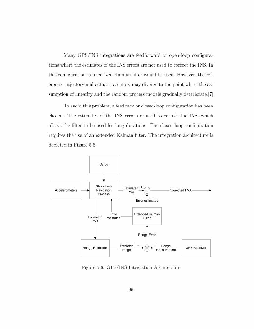
Many GPS/INS integrations are feedforward or open-loop configura-

tions where the estimates of the INS errors are not used to correct the INS. In

this configuration, a linearized Kalman filter would be used. However, the ref-

erence trajectory and actual trajectory may diverge to the point where the as-

sumption of linearity and the random process models gradually deteriorate.[7]

To avoid this problem, a feedback or closed-loop configuration has been

chosen. The estimates of the INS error are used to correct the INS, which

allows the filter to be used for long durations. The closed-loop configuration

requires the use of an extended Kalman filter. The integration architecture is

depicted in Figure 5.6.

Gyros

Accelerometers

Strapdown

Navigation

Process

Range Prediction GPS Receiver

Extended Kalman

FilterEstimated

PVA

Predicted

range

Range

measurement

Range Error

Estimated

PVA

Error

estimates

Error estimates

Corrected PVA

+-

+

+

Figure 5.6: GPS/INS Integration Architecture

96

One advantage of the closed-loop configuration is the ability to aid

the GPS tracking loops. This allows the GPS receiver to quickly re-acquire

satellites after loss of signal lock due to blockage, maneuvers or blackout during

re-entry.

In this dissertation, the GPS tracking loops are not simulated. The

simulated GPS receivers are able to acquire and track GPS SVs as soon as

they become visible. This would be the best case performance resulting from

aiding of the GPS tracking loops.

Three filters have been developed during this research: a GPS/INS

absolute navigation filter, a GPS/INS relative navigation filter, and a GPS-

only relative navigation filter. The details of these filters are described below.

5.2.1 Extended Kalman Filter Equations

The formulation of the extended Kalman filter equations is discussed

in detail in many textbooks, such as Brown and Hwang. [7] The equations are

summarized in this section. The general state and measurement models are

given by:

x(t) = f (x(t), t) + G (t)w (t) (5.62)

zk = h (xk) + vk (5.63)

where w (t) ∼ N (0, Q (t)) and vk ∼ N (0, Rk). In order to linearize the state

and measurement models, define the output and system matrices as:

Hk ≡ ∂h

∂x

∣∣∣∣x=x

F ≡ ∂f

∂x

∣∣∣∣x=x

(5.64)

97

The state and covariance propagation equations are:

x(t) = f (x(t), t) (5.65)

Φ (tk, tk−1) = F (tk−1) Φ (tk, tk−1) (5.66)

P−k = Φ (tk, tk−1) P+

k−1ΦT (tk, tk−1) + Qk (5.67)

The Kalman gain is computed by:

Kk = P−k HT

k

[HkP

−k HT

k + Rk

]−1(5.68)

The measurement update equations are:

x+k = x−k + Kk

[yk − h

(x−k

)](5.69)

P+k =

[I −KkHk

(x−k

)]P−

k (5.70)

5.2.2 Numerical Integration of INS Solution

In a complementary GPS/INS filter, the reference trajectory is sup-

plied by integrating the equations of motion using the gyro and accelerometer

measurements. The following classical fourth-order Runge-Kutta equation is

used in the EKF for this integration:

xi+1 = xi +∆t

6(k1 + 2k2 + 2k3 + k4) (5.71)

where:

k1 = f(ti,xi) (5.72)

k2 = f(ti +∆t

2,xi +

∆t

2k1) (5.73)

98

k3 = f(ti +∆t

2,xi +

∆t

2k2) (5.74)

k4 = f(ti + ∆t,xi + ∆tk3) (5.75)

This algorithm requires that the function being integrated be evaluated

at the ends of the integration interval and half way in between. Therefore, the

integration interval, ∆t, is defined to be twice the gyro and accelerometer

sampling interval:

∆t = 2δt (5.76)

In order to compute k1 through k4, the gyro measurements must be converted

to estimates of the angular velocity and the accelerometer measurements must

be converted to estimates of specific force at times tl−2, tl−1 and tl. This

process is discussed in detail in Jekeli [22] and summarized below.

For the gyro measurements, a Taylor series expansion of the angular

velocity vector about tl−2 yields:

ω (t) = ωl−2 + ωl−2 [t− tl−2] + O(∆t2

), |t− tl−2| ≤ ∆t (5.77)

Substituting (5.77) into (5.25) and assuming the angular velocity and

angular velocity rate are constant over the sampling interval yields:

δθl−1 = ωl−2δt +1

2ωl−2δt

2 + O(∆t3

)(5.78)

δθl = ωl−2δt +3

2ωl−2δt

2 + O(∆t3

)(5.79)

99

Ignoring the higher order terms and solving (5.78) and (5.79) for ωl−2 and

ωl−2 leads to:

ωl−2 =1

2δt(3δθl−1 − δθl) (5.80)

ωl−2 =1

δt2(δθl − δθl−1) (5.81)

Using (5.80) and (5.81) in (5.77) provides the following estimated quantities:

ωl−2 =3 δθl−1 − δθl

∆t(5.82)

ωl−1 =δθl−1 + δθl

∆t(5.83)

ωl =3 δθl − δθl−1

∆t(5.84)

Following the same procedure for the accelerometer measurements yields:

fl−2 ∆t = 3 δvl−1 − δvl (5.85)

fl−1 ∆t = δvl−1 + δvl (5.86)

fl ∆t = 3 δvl − δvl−1 (5.87)

5.2.2.1 Analysis of Integration Algorithm Accuracy

The algorithm errors are a function of the integration step size and ve-

hicle dynamics. It is desirable to choose an integration step size that results in

errors that are much smaller than the incoming measured data. The algorithm

errors for both the attitude and velocity integration algorithms are examined

in this section.

100

The angular error per unit time for the Runge-Kutta algorithm can be

approximated by: [22]

δω ≈ ωm+1 ∆tm+1

(m + 1)!(5.88)

where m is the order of the algorithm. At the ISS orbit, the angular rate of

the body frame with respect to the inertial frame is 0.0011 rad/s. With a ∆t=

1 s and a fourth-order algorithm, the angular rate error is 3.23×10−12 deg/hr,

which is well below the SIGI gyro bias of 0.0035 deg/hr.

The acceleration error for the integration algorithm can be approxi-

mated by: [22]

δa ≈ ωm a ∆tm

(m + 1)!(5.89)

During the rendezvous scenario, the largest non-gravitational acceler-

ation is due to thrust, which is about 0.1 m/s2. With a ∆t= 1 s and a

fourth-order algorithm, the acceleration error is 1.38 × 10−15 m/s2, which is

well below the SIGI accelerometer bias of 30 µg or 2.9×10−5 m/s2. Therefore,

an integration step size of one second is clearly adequate.

5.2.3 State Propagation Models

This section provides the mathematical models used to propagate the

states in the absolute and relative navigation filters.

101

5.2.3.1 Earth Gravity Model

The gravity model used in the absolute and relative navigation filters

includes the effects of the J2 zonal coefficient. Therefore, the gravitational

potential function is:

U =µ

r− µR2

EJ2

[3z2

2r5 − 12r3

](5.90)

and the acceleration due to gravity is given by:

∇U =

−µxr3

[1− 3

2

(µ

RE

)2

J2

(5z2

r2 − 1)]

−µyr3

[1− 3

2

(µ

RE

)2

J2

(5z2

r2 − 1)]

−µzr3

[1− 3

2

(µ

RE

)2

J2

(5z2

r2 − 3)]

(5.91)

5.2.3.2 Atmospheric Drag Model

In the GPS/INS relative navigation filter, it is assumed that the ISS

does not have an INS to measure the effects of atmospheric drag. In the GPS-

only relative navigation filter, neither vehicle can measure the effects of drag.

Therefore, an atmospheric drag model is required. The acceleration due to

atmospheric drag, fdrag, is computed using:

fdrag = −1

2

CDA

mρV 2

rel

Vrel

‖Vrel‖ (5.92)

where CD is the drag coefficient, A is the reference surface area, m is the mass.

The atmospheric density, ρ, is computed using an exponential atmospheric

density model, which is described in Vallado [42].

102

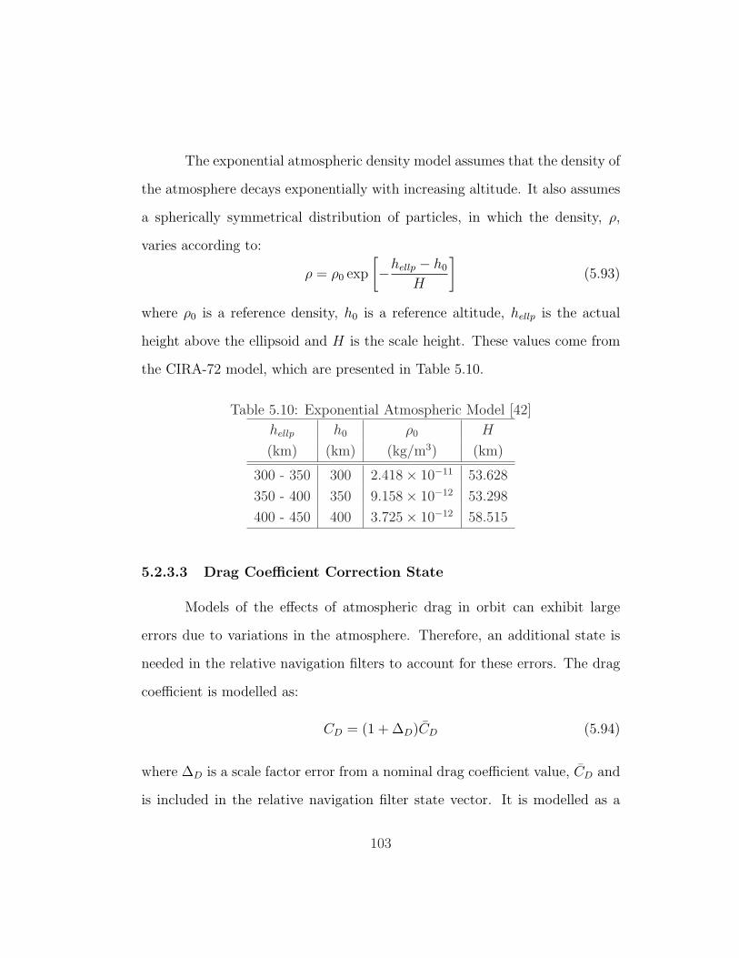
The exponential atmospheric density model assumes that the density of

the atmosphere decays exponentially with increasing altitude. It also assumes

a spherically symmetrical distribution of particles, in which the density, ρ,

varies according to:

ρ = ρ0 exp

[−hellp − h0

H

](5.93)

where ρ0 is a reference density, h0 is a reference altitude, hellp is the actual

height above the ellipsoid and H is the scale height. These values come from

the CIRA-72 model, which are presented in Table 5.10.

Table 5.10: Exponential Atmospheric Model [42]

hellp h0 ρ0 H

(km) (km) (kg/m3) (km)

300 - 350 300 2.418× 10−11 53.628

350 - 400 350 9.158× 10−12 53.298

400 - 450 400 3.725× 10−12 58.515

5.2.3.3 Drag Coefficient Correction State

Models of the effects of atmospheric drag in orbit can exhibit large

errors due to variations in the atmosphere. Therefore, an additional state is

needed in the relative navigation filters to account for these errors. The drag

coefficient is modelled as:

CD = (1 + ∆D)CD (5.94)

where ∆D is a scale factor error from a nominal drag coefficient value, CD and

is included in the relative navigation filter state vector. It is modelled as a

103

first-order Gauss-Markov process with the following time constant: [13]

τD = 180000 sec (5.95)

and standard deviation of:

σD = 0.5 (5.96)

5.2.3.4 Gyro and Accelerometer Bias States

The gyro and accelerometer bias states are modelled as first-order

Gauss-Markov processes. The parameters presented in Table 5.8 were used

for the SIGI cases.

5.2.3.5 GPS Receiver Clock States

The GPS receiver clock bias and drift model used in the filter is the

same model used to generate the GPS measurements, which is described in

Section 5.1.3.3.

5.2.3.6 Ionospheric Delay State

The state being estimated by the filter is the ionospheric scale factor,

denoted by ∆IV , where

IV = (1 + ∆IV ) IV (5.97)

and IV represents an average value of IV , whose value is recommended to be

5.2 m by Ebinuma. [13] The ionospheric scale factor state is modelled as a

104

first order Gauss-Markov process with a time constant of:

τIV = 2000 s (5.98)

and standard deviation of

σ∆IV= 0.82 (5.99)

5.2.3.7 URE State

The filter estimates the GPS user range error for each GPS SV. Usually

there would be one state per channel in the GPS receiver to save memory and

computation time, however, for this simulation, there is one state for each

GPS SV in the active constellation.

The user range error for each GPS SV is modelled as a first order

Gauss-Markov process with:

σURE =√

1.22 + 3.22 + 4.52 + 3.362 = 6.57 m (5.100)

and the recommended time constant from Ebinuma is: [13]

τURE = 7200 s (5.101)

5.2.3.8 Integer Ambiguity State

The single-difference integer ambiguity is estimated by the relative nav-

igation filters. Although the ambiguity is an integer, the filter estimates a real

number. Since the integer ambiguity is a fixed constant value while the carrier

105

phase is observed (if no cycle slip occurs), the single-difference integer ambi-

guity is also a fixed constant and is modelled as a random-walk process with

a standard deviation of:[13]

σλN = 0.0002 m (5.102)

A small amount of process noise is given to allow for innovations in the

estimate to occur over time.

5.2.4 Process Noise Covariance

The continuous time process noise covariance matrix is denoted by Q(t).

The values for Q(t) are provided in Chapter 6. The discrete equivalent of the

process noise covariance used in the discrete Kalman filter can be expressed

as:

Qk =

∫ tk+1

tk

Φ (tk+1, τ)G (τ)Q (τ)GT (τ) ΦT (tk+1, τ) dτ (5.103)

Since G(t) and Q(t) are constants and the dynamics are slowly varying,

the following approximation is used:

Qk ≈ Φ (tk+1, tk)GQGT ΦT (tk+1, tk) ∆t (5.104)

In the relative navigation filters, it is assumed that the two spacecraft

are orbiting near each other. Therefore the uncertainties in the spacecraft

dynamics are significantly correlated. If the matrix Qchaser represents the 6×6

covariance matrix for the position and velocity states for the chaser and QISS

106

represents the position and velocity covariance matrix for the ISS, then there

is an off-diagonal block matrix, QAB defined by:

QAB(k, l) = ρQ

√Qchaser(k, l)QISS(k, l) (5.105)

where Q(k, l) represents the kth row and lth column element of the matrix Q

and ρQ is the process noise correlation coefficient.

5.2.5 Measurement Models

The absolute navigation filter processes GPS C/A code pseudorange

measurements. The relative navigation filters process GPS C/A code pseu-

dorange measurements from the chaser and the ISS. The relative navigation

filters also process single difference carrier phase measurements formed by sub-

tracting carrier phase measurements from the ISS from measurements from the

chaser.

While many systems use double differenced measurements to remove

the GPS receiver clock bias, this would reduce the number of measurements

available to the filter. This is especially important when GPS signals can be

blocked. Fortunately, there is no need to use double difference measurements

because the filter can estimate the GPS receiver clock bias.

The measurement update processes a single measurement at a time as

they come in. If there is a carrier phase measurement from both vehicles with

the same time tag and using the same GPS SV, the single difference carrier

phase measurement is formed and processed. The relative navigation filters

107

do not enforce any common satellite requirement. Furthermore, it is assumed

that there is no delay in receiving or processing measurements from the ISS

by the chaser.

The measured range from the j th GPS satellite to the vehicle at time

tk can be represented by the following non-linear equation:

zj(tk) = hj(x, tk) + v(tk) (5.106)

where v(tk) is a zero-mean, white Gaussian noise process of strength R repre-

senting random range measurement noise. The linearized scalar measurements

presented to the filter are:

δzj(tk) = zj(tk)− hj(x, tk) (5.107)

The measurement model for C/A code pseudorange measurements is:

hj (x, tk) = ρ +

(1− ρ

c

)bc + ∆URE + ∆iono (5.108)

and for single difference carrier phase measurements is:

hj (x, tk) = ρ +

(1− ρchaser

c

)bcchaser

−(

1− ρISS

c

)bcISS

+ λN (5.109)

5.2.5.1 Measurement Noise Covariance

The C/A code pseudorange and carrier phase range measurement er-

rors are assumed to be zero-mean, white Gaussian random numbers with the

108

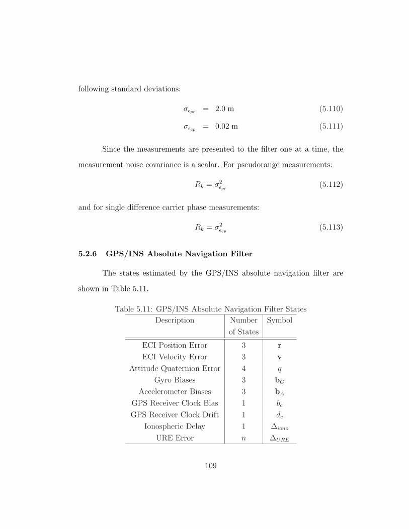
following standard deviations:

σεpr = 2.0 m (5.110)

σεcp = 0.02 m (5.111)

Since the measurements are presented to the filter one at a time, the

measurement noise covariance is a scalar. For pseudorange measurements:

Rk = σ2εpr

(5.112)

and for single difference carrier phase measurements:

Rk = σ2εcp

(5.113)

5.2.6 GPS/INS Absolute Navigation Filter

The states estimated by the GPS/INS absolute navigation filter are

shown in Table 5.11.

Table 5.11: GPS/INS Absolute Navigation Filter States

Description Number Symbol

of States

ECI Position Error 3 r

ECI Velocity Error 3 v

Attitude Quaternion Error 4 q

Gyro Biases 3 bG

Accelerometer Biases 3 bA

GPS Receiver Clock Bias 1 bc

GPS Receiver Clock Drift 1 dc

Ionospheric Delay 1 ∆iono

URE Error n ∆URE

109

5.2.7 GPS/INS Relative Navigation Filter

The states estimated by the GPS/INS relative navigation filter are


Table 5.12: GPS/INS Relative Navigation Filter States


of States

Chaser ECI Position Error 3 r

Chaser ECI Velocity Error 3 v

Attitude Quaternion Error 4 q

Gyro Biases 3 bG

Accelerometer Biases 3 bA

Chaser GPS Receiver Clock Bias 1 bc

Chaser GPS Receiver Clock Drift 1 dc


URE Error n ∆URE

ISS ECI Position Error 3 r

ISS ECI Velocity Error 3 v

ISS GPS Receiver Clock Bias 1 bc

ISS GPS Receiver Clock Drift 1 dc

ISS Drag Coefficient 1 ∆D

Integer Ambiguities n λN

110

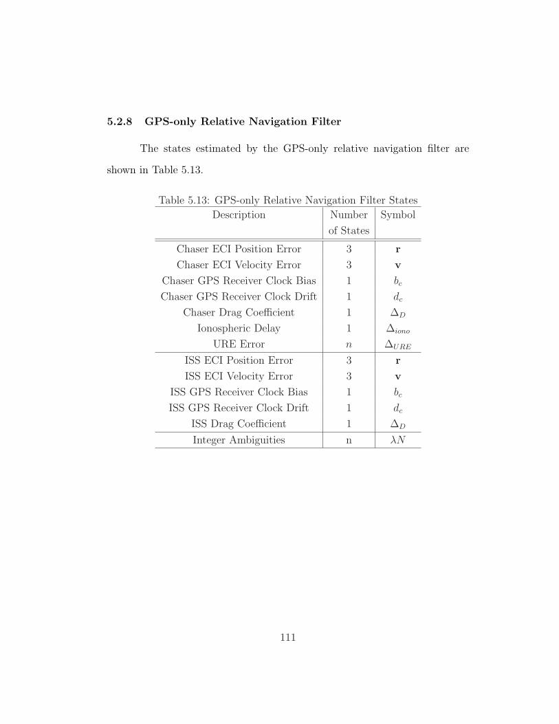
5.2.8 GPS-only Relative Navigation Filter

The states estimated by the GPS-only relative navigation filter are


Table 5.13: GPS-only Relative Navigation Filter States


of States

Chaser ECI Position Error 3 r

Chaser ECI Velocity Error 3 v

Chaser GPS Receiver Clock Bias 1 bc

Chaser GPS Receiver Clock Drift 1 dc

Chaser Drag Coefficient 1 ∆D


URE Error n ∆URE

ISS ECI Position Error 3 r

ISS ECI Velocity Error 3 v

ISS GPS Receiver Clock Bias 1 bc

ISS GPS Receiver Clock Drift 1 dc

ISS Drag Coefficient 1 ∆D

Integer Ambiguities n λN

111

Chapter 6

GPS/INS Simulation Results

The results of simulation runs using the absolute navigation filters and

relative navigation filters are discussed in this chapter.

6.1 Absolute Navigation

When a spacecraft is not in close proximity to any other spacecraft,

accurate absolute navigation may be required in order to perform a de-orbit

maneuver or to satisfy other mission objectives. Therefore, a brief discussion

of the results of the GPS/INS absolute navigation filter runs is presented in

this section.

6.1.1 C/A Code vs. Carrier Phase Measurements

The decision of whether to use C/A code or carrier phase measurements

was addressed early in the design process using a preliminary version of the

GPS/INS simulation. In this version, both the chaser and ISS are moving in

a two-body gravity field with no other forces acting. The chaser is initially

placed on a trajectory designed to rendezvous the ISS in a simple two-impulse

rendezvous scenario. The simulation begins just after the first impulse and

112

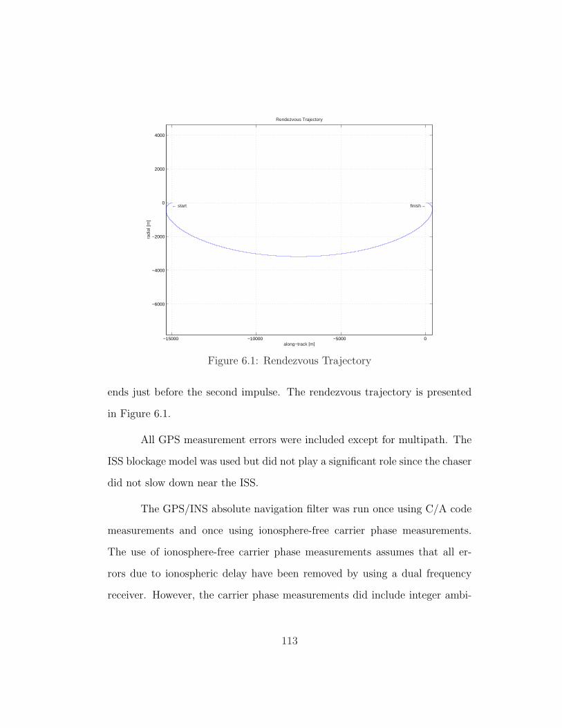
−15000 −10000 −5000 0

−6000

−4000

−2000

0

2000

4000

along−track [m]

radi

al [m

]

← start finish→


Figure 6.1: Rendezvous Trajectory

ends just before the second impulse. The rendezvous trajectory is presented

in Figure 6.1.

All GPS measurement errors were included except for multipath. The

ISS blockage model was used but did not play a significant role since the chaser

did not slow down near the ISS.

The GPS/INS absolute navigation filter was run once using C/A code

measurements and once using ionosphere-free carrier phase measurements.

The use of ionosphere-free carrier phase measurements assumes that all er-

rors due to ionospheric delay have been removed by using a dual frequency

receiver. However, the carrier phase measurements did include integer ambi-

113

guities, which were estimated by the modified GPS/INS absolute navigation

filter. The results of both runs are shown in Figures 6.2 and 6.3.

These runs show that although carrier phase measurements are more

precise than C/A code measurements, the GPS/INS filter is not able to esti-

mate the integers well enough to take advantage of the carrier phase measure-

ment precision. Therefore, the use of carrier phase measurements for absolute

navigation provides little additional information, since additional states are

required to estimate the integers. For this reason, the absolute navigation

filter was designed to use pseudorange measurements for this application.

0 1000 2000 3000 4000 5000 6000−10

−5

0

5

10

x er

ror

[m]

ECI Position Errors

C/A CodeCarrier Phase

0 1000 2000 3000 4000 5000 6000−10

−5

0

5

10

y er

ror

[m]

0 1000 2000 3000 4000 5000 6000−10

−5

0

5

10

time [s]

z er

ror

[m]

Figure 6.2: Comparision of Absolute Position Errors Using C/A Code andCarrier Phase Measurements

114

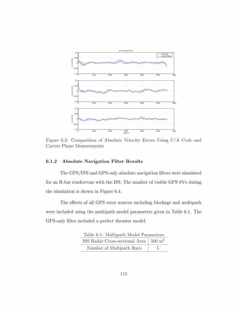
0 1000 2000 3000 4000 5000 6000−0.1

−0.05

0

0.05

0.1

v x err

or [m

/s]

ECI Velocity Errors

C/A CodeCarrier Phase

0 1000 2000 3000 4000 5000 6000−0.1

−0.05

0

0.05

0.1

v y err

or [m

/s]

0 1000 2000 3000 4000 5000 6000−0.1

−0.05

0

0.05

0.1

time [s]

v z err

or [m

]

Figure 6.3: Comparision of Absolute Velocity Errors Using C/A Code andCarrier Phase Measurements

6.1.2 Absolute Navigation Filter Results

The GPS/INS and GPS-only absolute navigation filters were simulated

for an R-bar rendezvous with the ISS. The number of visible GPS SVs during

the simulation is shown in Figure 6.4.

The effects of all GPS error sources including blockage and multipath

were included using the multipath model parameters given in Table 6.1. The

GPS-only filter included a perfect thruster model.

Table 6.1: Multipath Model Parameters

ISS Radar Cross-sectional Area 500 m2

Number of Multipath Rays 5

115

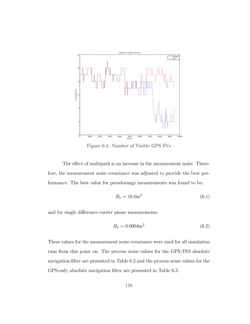
0 1000 2000 3000 4000 5000 6000 7000 8000 9000 100000

2

4

6

8

10

12

time [s]

# of

vis

ible

SV

s

Number of Visible GPS SVs

ChaserISS

Figure 6.4: Number of Visible GPS SVs

The effect of multipath is an increase in the measurement noise. There-

fore, the measurement noise covariance was adjusted to provide the best per-

formance. The best value for pseudorange measurements was found to be:

Rk = 16.0m2 (6.1)

and for single difference carrier phase measurements:

Rk = 0.0004m2 (6.2)

These values for the measurement noise covariance were used for all simulation

runs from this point on. The process noise values for the GPS/INS absolute

navigation filter are presented in Table 6.2 and the process noise values for the

GPS-only absolute navigation filter are presented in Table 6.3.

116

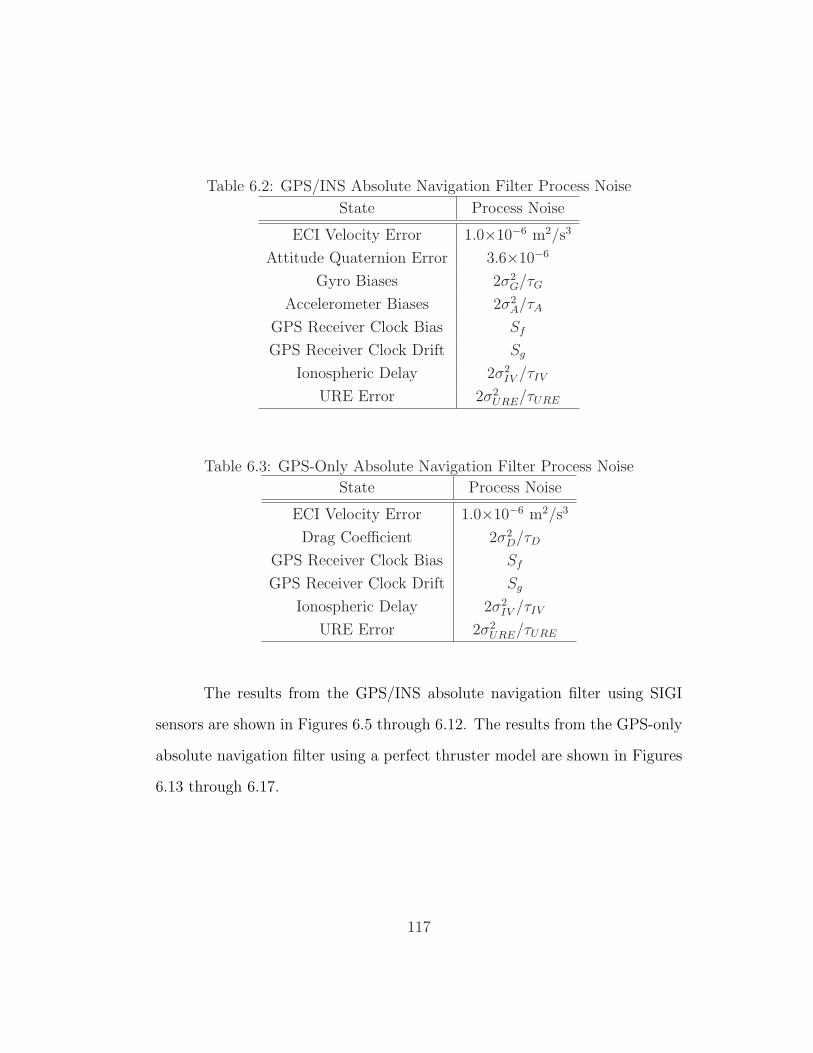
Table 6.2: GPS/INS Absolute Navigation Filter Process Noise

State Process Noise

ECI Velocity Error 1.0×10−6 m2/s3

Attitude Quaternion Error 3.6×10−6

Gyro Biases 2σ2G/τG

Accelerometer Biases 2σ2A/τA

GPS Receiver Clock Bias Sf

GPS Receiver Clock Drift Sg

Ionospheric Delay 2σ2IV /τIV

URE Error 2σ2URE/τURE

Table 6.3: GPS-Only Absolute Navigation Filter Process Noise

State Process Noise

ECI Velocity Error 1.0×10−6 m2/s3

Drag Coefficient 2σ2D/τD

GPS Receiver Clock Bias Sf

GPS Receiver Clock Drift Sg

Ionospheric Delay 2σ2IV /τIV

URE Error 2σ2URE/τURE

The results from the GPS/INS absolute navigation filter using SIGI

sensors are shown in Figures 6.5 through 6.12. The results from the GPS-only

absolute navigation filter using a perfect thruster model are shown in Figures

6.13 through 6.17.

117

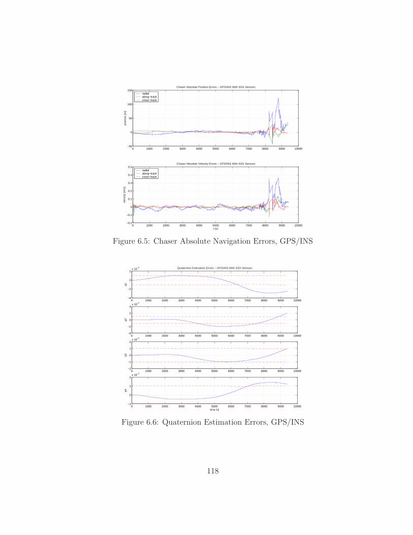
0 1000 2000 3000 4000 5000 6000 7000 8000 9000 10000−50

0

50

100

150

posi

tion

[m]

Chaser Absolute Position Errors − GPS/INS With SIGI Sensors

radialalong−trackcross−track

0 1000 2000 3000 4000 5000 6000 7000 8000 9000 10000−0.2

−0.1

0

0.1

0.2

0.3

0.4

0.5

t [s]

velo

city

[m/s

]

Chaser Absolute Velocity Errors − GPS/INS With SIGI Sensors


Figure 6.5: Chaser Absolute Navigation Errors, GPS/INS

0 1000 2000 3000 4000 5000 6000 7000 8000 9000 10000−4

−2

0

2x 10

−3

q1

Quaternion Estimation Errors − GPS/INS With SIGI Sensors

0 1000 2000 3000 4000 5000 6000 7000 8000 9000 10000−4

−2

0

2

4x 10

−3

q2

0 1000 2000 3000 4000 5000 6000 7000 8000 9000 10000−2

−1

0

1

2x 10

−3

q3

0 1000 2000 3000 4000 5000 6000 7000 8000 9000 10000−1

0

1

2x 10

−3

time [s]

q4

Figure 6.6: Quaternion Estimation Errors, GPS/INS

118

0 1000 2000 3000 4000 5000 6000 7000 8000 9000 10000−3

−2

−1

0

1

2x 10

−8

x gy

ro [r

ad/s

]

Gyro Bias Estimation Errors − GPS/INS With SIGI Sensors

0 1000 2000 3000 4000 5000 6000 7000 8000 9000 10000−2

0

2

4

6x 10

−8

y gy

ro [r

ad/s

]

0 1000 2000 3000 4000 5000 6000 7000 8000 9000 10000−2

0

2

4

6x 10

−8

time [s]

z gy

ro [r

ad/s

]

Figure 6.7: Gyro Bias Estimation Errors, GPS/INS

0 1000 2000 3000 4000 5000 6000 7000 8000 9000 10000

−2

−1

0

1

2

x 10−4

x ac

cel [

m/s

2 ]

Accelerometer Bias Estimation Errors − GPS/INS With SIGI Sensors

0 1000 2000 3000 4000 5000 6000 7000 8000 9000 10000

−2

−1

0

1

2

x 10−4

y ac

cel [

m/s

2 ]

0 1000 2000 3000 4000 5000 6000 7000 8000 9000 10000

−2

−1

0

1

2

3x 10

−4

time [s]

z ac

cel [

m/s

2 ]

Figure 6.8: Accelerometer Bias Estimation Errors, GPS/INS

119

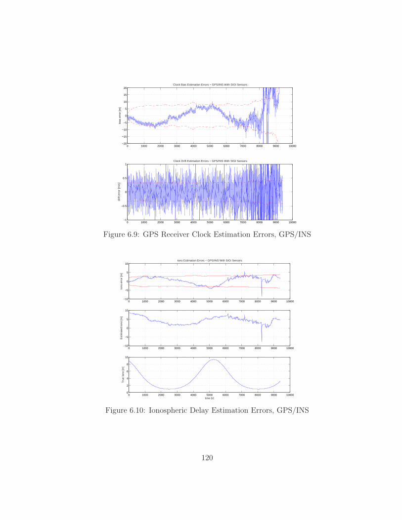
0 1000 2000 3000 4000 5000 6000 7000 8000 9000 10000−20

−15

−10

−5

0

5

10

15

20

bias

err

or [m

]

Clock Bias Estimation Errors − GPS/INS With SIGI Sensors

0 1000 2000 3000 4000 5000 6000 7000 8000 9000 10000−1

−0.5

0

0.5

1

drift

err

or [m

/s]

Clock Drift Estimation Errors − GPS/INS With SIGI Sensors

Figure 6.9: GPS Receiver Clock Estimation Errors, GPS/INS

0 1000 2000 3000 4000 5000 6000 7000 8000 9000 10000−10

−5

0

5

10

Iono

err

or [m

]

Iono Estimation Errors − GPS/INS With SIGI Sensors

0 1000 2000 3000 4000 5000 6000 7000 8000 9000 10000−10

−5

0

5

10

Est

imat

ed Io

no [m

]

0 1000 2000 3000 4000 5000 6000 7000 8000 9000 100000

2

4

6

8

10

time [s]

Tru

e Io

no [m

]

Figure 6.10: Ionospheric Delay Estimation Errors, GPS/INS

120

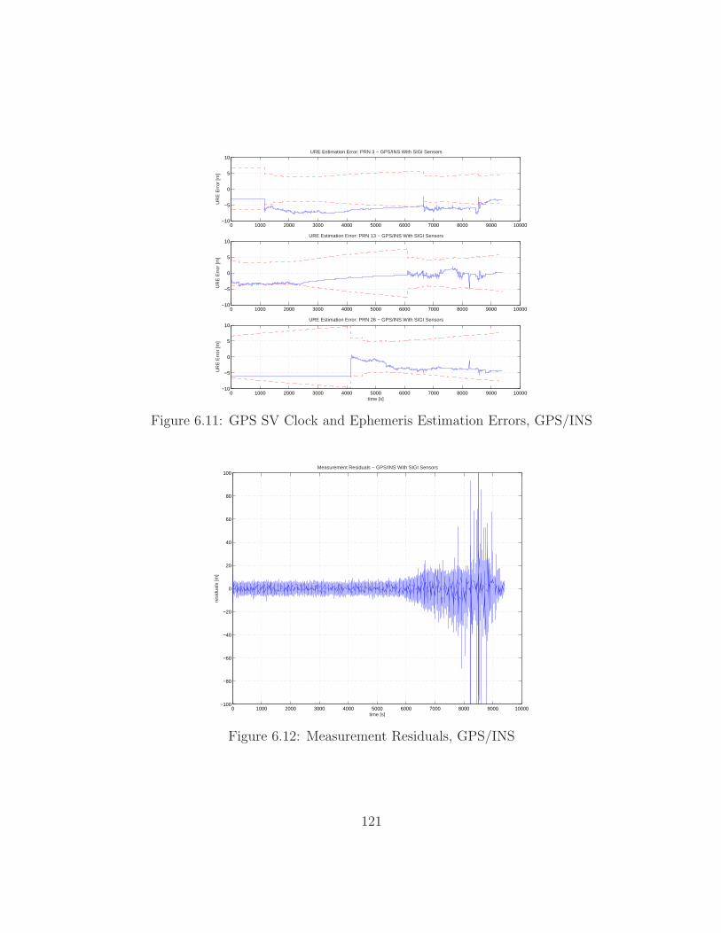
0 1000 2000 3000 4000 5000 6000 7000 8000 9000 10000−10

−5

0

5

10

UR

E E

rror

[m]

URE Estimation Error: PRN 3 − GPS/INS With SIGI Sensors

0 1000 2000 3000 4000 5000 6000 7000 8000 9000 10000−10

−5

0

5

10

UR

E E

rror

[m]


0 1000 2000 3000 4000 5000 6000 7000 8000 9000 10000−10

−5

0

5

10

time [s]

UR

E E

rror

[m]


Figure 6.11: GPS SV Clock and Ephemeris Estimation Errors, GPS/INS

0 1000 2000 3000 4000 5000 6000 7000 8000 9000 10000−100

−80

−60

−40

−20

0

20

40

60

80

100

time [s]

resi

dual

s [m

]

Measurement Residuals − GPS/INS With SIGI Sensors

Figure 6.12: Measurement Residuals, GPS/INS

121

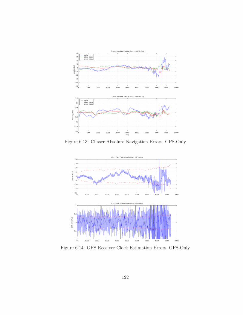
0 1000 2000 3000 4000 5000 6000 7000 8000 9000 10000−50

−40

−30

−20

−10

0

10

20

30

40

posi

tion

[m]

Chaser Absolute Position Errors − GPS−Only


0 1000 2000 3000 4000 5000 6000 7000 8000 9000 10000−0.2

−0.15

−0.1

−0.05

0

0.05

0.1

0.15

t [s]

velo

city

[m/s

]

Chaser Absolute Velocity Errors − GPS−Only


Figure 6.13: Chaser Absolute Navigation Errors, GPS-Only

0 1000 2000 3000 4000 5000 6000 7000 8000 9000 10000−20

−15

−10

−5

0

5

10

15

20

bias

err

or [m

]

Clock Bias Estimation Errors − GPS−Only

0 1000 2000 3000 4000 5000 6000 7000 8000 9000 10000−1

−0.5

0

0.5

1

drift

err

or [m

/s]

Clock Drift Estimation Errors − GPS−Only

Figure 6.14: GPS Receiver Clock Estimation Errors, GPS-Only

122

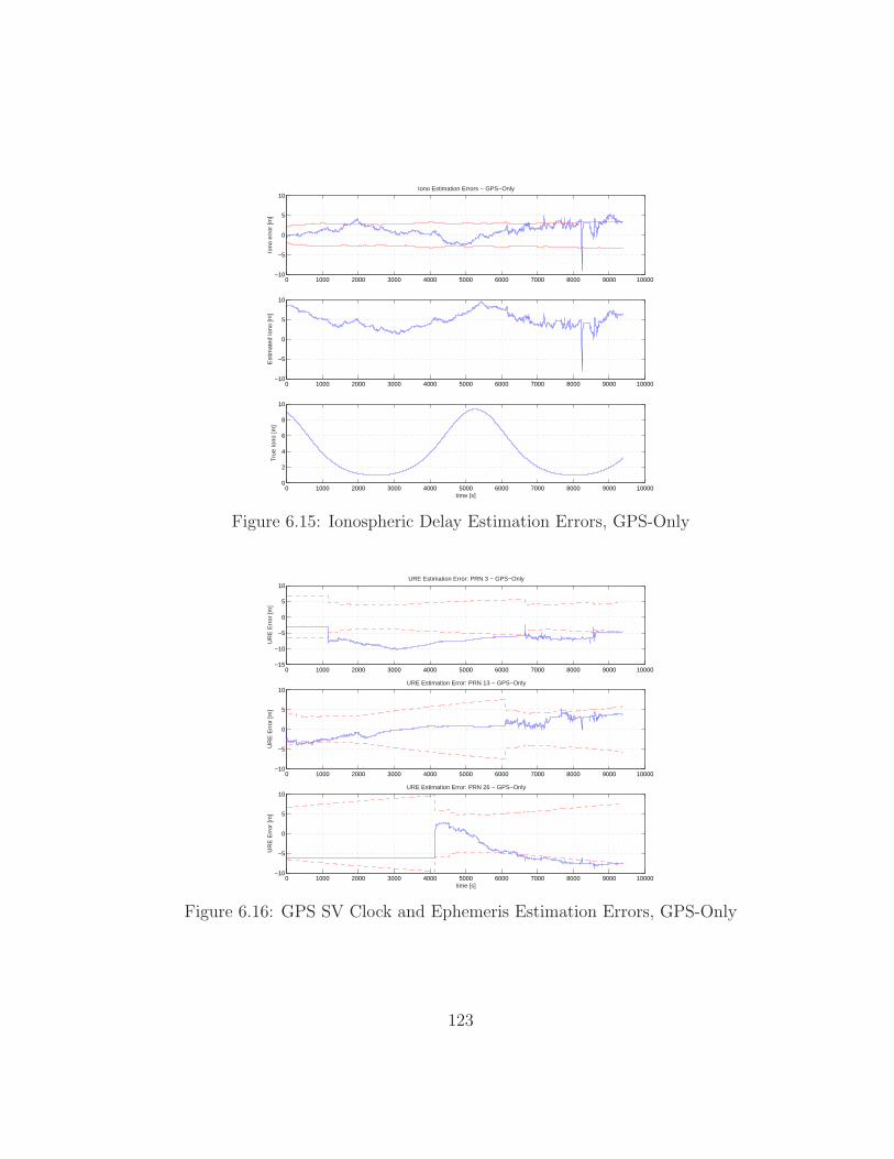
0 1000 2000 3000 4000 5000 6000 7000 8000 9000 10000−10

−5

0

5

10

Iono

err

or [m

]

Iono Estimation Errors − GPS−Only

0 1000 2000 3000 4000 5000 6000 7000 8000 9000 10000−10

−5

0

5

10

Est

imat

ed Io

no [m

]

0 1000 2000 3000 4000 5000 6000 7000 8000 9000 100000

2

4

6

8

10

time [s]

Tru

e Io

no [m

]

Figure 6.15: Ionospheric Delay Estimation Errors, GPS-Only

0 1000 2000 3000 4000 5000 6000 7000 8000 9000 10000−15

−10

−5

0

5

10

UR

E E

rror

[m]

URE Estimation Error: PRN 3 − GPS−Only

0 1000 2000 3000 4000 5000 6000 7000 8000 9000 10000−10

−5

0

5

10

UR

E E

rror

[m]


0 1000 2000 3000 4000 5000 6000 7000 8000 9000 10000−10

−5

0

5

10

time [s]

UR

E E

rror

[m]


Figure 6.16: GPS SV Clock and Ephemeris Estimation Errors, GPS-Only

123

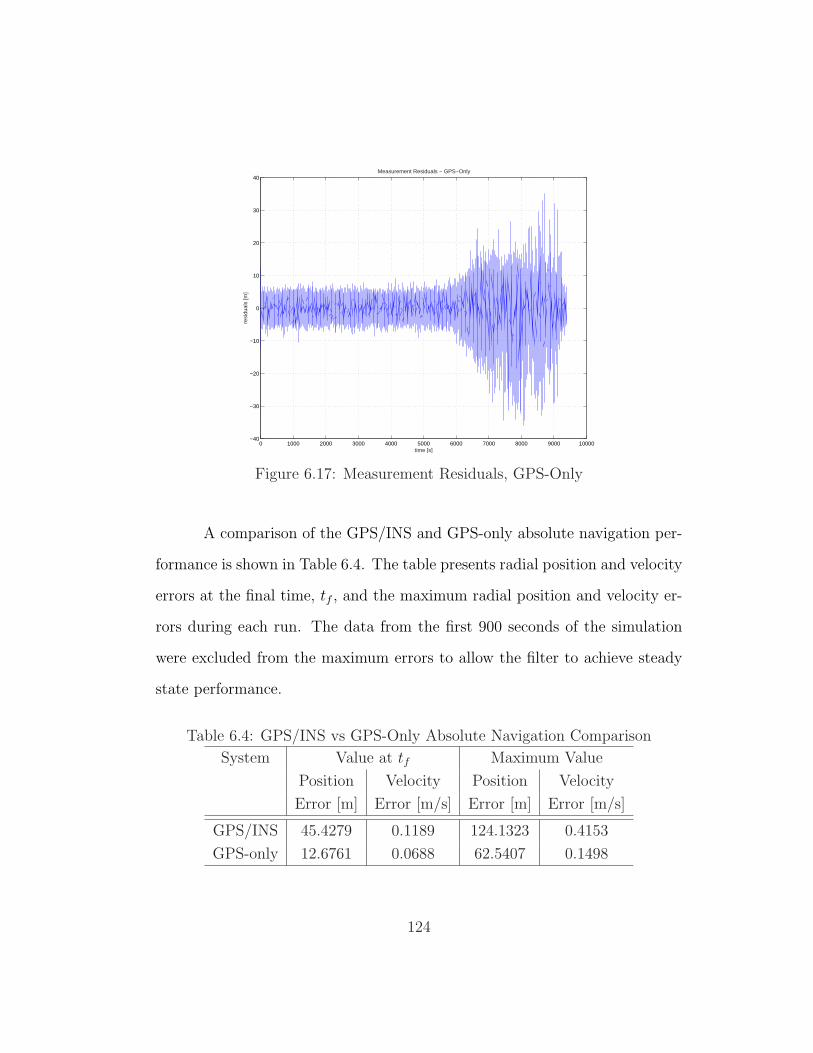
0 1000 2000 3000 4000 5000 6000 7000 8000 9000 10000−40

−30

−20

−10

0

10

20

30

40

time [s]

resi

dual

s [m

]

Measurement Residuals − GPS−Only

Figure 6.17: Measurement Residuals, GPS-Only

A comparison of the GPS/INS and GPS-only absolute navigation per-

formance is shown in Table 6.4. The table presents radial position and velocity

errors at the final time, tf , and the maximum radial position and velocity er-

rors during each run. The data from the first 900 seconds of the simulation

were excluded from the maximum errors to allow the filter to achieve steady

state performance.

Table 6.4: GPS/INS vs GPS-Only Absolute Navigation Comparison

System Value at tf Maximum Value

Position Velocity Position Velocity

Error [m] Error [m/s] Error [m] Error [m/s]

GPS/INS 45.4279 0.1189 124.1323 0.4153

GPS-only 12.6761 0.0688 62.5407 0.1498

124

The GPS-only filter with a perfect thruster model provided better ab-

solute navigation performance than the GPS/INS using SIGI sensors. In this

case, the dynamics model of the GPS-only filter provides a better reference

trajectory than the GPS/INS. One reason for this is the acceleration due to

atmospheric drag is lower than accelerometer sensor noise. Therefore, the ac-

celerometer is not able to accurately measure the acceleration due to drag.

Another reason is the accuracy of the accelerometer bias estimates in the

GPS/INS filter is only about 10−4 m/s2, which integrates into position and

velocity errors.

Relative navigation performance becomes more important than abso-

lute navigation performance during rendezvous. The GPS/INS and GPS-only

absolute navigation filters demonstrated 10-meter level absolute navigation

performance when there is no blockage or multipath from the ISS. This is

adequate for most on-orbit operations. Therefore, no further studies of the

absolute navigation filters were made.

6.2 Relative Navigation

During proximity operations, especially during rendezvous, accurate

relative navigation is required for safety and to minimize propellant use. There

are many factors which influence the accuracy of a GPS/INS-based relative

navigation system, including: what information is exchanged between vehicles,

the GPS constellation geometry, the rendezvous approach direction, thruster

model accuracy, filter tuning, accelerometer and gyroscope accuracy, level of

125

GPS multipath, and the GPS antenna field of view. The effect of each of these

factors is discussed in this section.

6.2.1 State Vector vs. Measurement Differencing

One of the first decisions to be made in designing a GPS relative navi-

gation system is whether to exchange state vector information or measurement

information. While it may be more convenient and efficient to exchange state

information, it may not provide the relative navigation accuracy required.

This decision was addressed using the preliminary version of the GPS/INS

simulation discussed in Section 6.1.1.

In order to simulate the state vector information exchange option, the

GPS/INS absolute navigation filter was run once for the chaser vehicle and

once for the ISS. The resulting absolute navigation states were differenced to

obtain a relative navigation state, which was compared to the true relative

navigation state. The results of this run are presented in Figures 6.18 and

6.19.

In order to simulate the measurement information exchange option, the

GPS/INS relative navigation filter was used to process C/A code from both

the chaser and ISS and single difference carrier phase measurements. The

GPS/INS relative navigation filter outputs the absolute navigation states of

the chaser and ISS, which were differenced to obtain a relative navigation state.

The relative navigation state was compared to the true relative navigation

state. The results of this run are presented in Figures 6.20 and 6.21.

126

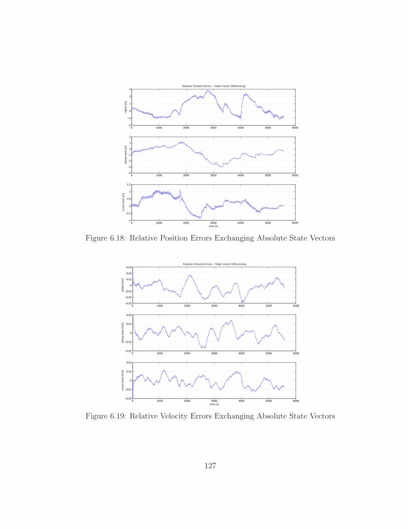
0 1000 2000 3000 4000 5000 6000−2

−1

0

1

2

3

radi

al [m

]

Relative Position Errors − State Vector Differencing

0 1000 2000 3000 4000 5000 6000−4

−3

−2

−1

0

1

2

alon

g tr

ack

[m]

0 1000 2000 3000 4000 5000 6000−1

−0.5

0

0.5

1

1.5

time [s]

cros

s tr

ack

[m]

Figure 6.18: Relative Position Errors Exchanging Absolute State Vectors

0 1000 2000 3000 4000 5000 6000−0.03

−0.02

−0.01

0

0.01

0.02

0.03

radi

al [m

/s]

Relative Velocity Errors − State Vector Differencing

0 1000 2000 3000 4000 5000 6000−0.02

−0.01

0

0.01

0.02

alon

g tr

ack

[m/s

]

0 1000 2000 3000 4000 5000 6000−0.02

−0.01

0

0.01

0.02

time [s]

cros

s tr

ack

[m/s

]

Figure 6.19: Relative Velocity Errors Exchanging Absolute State Vectors

127

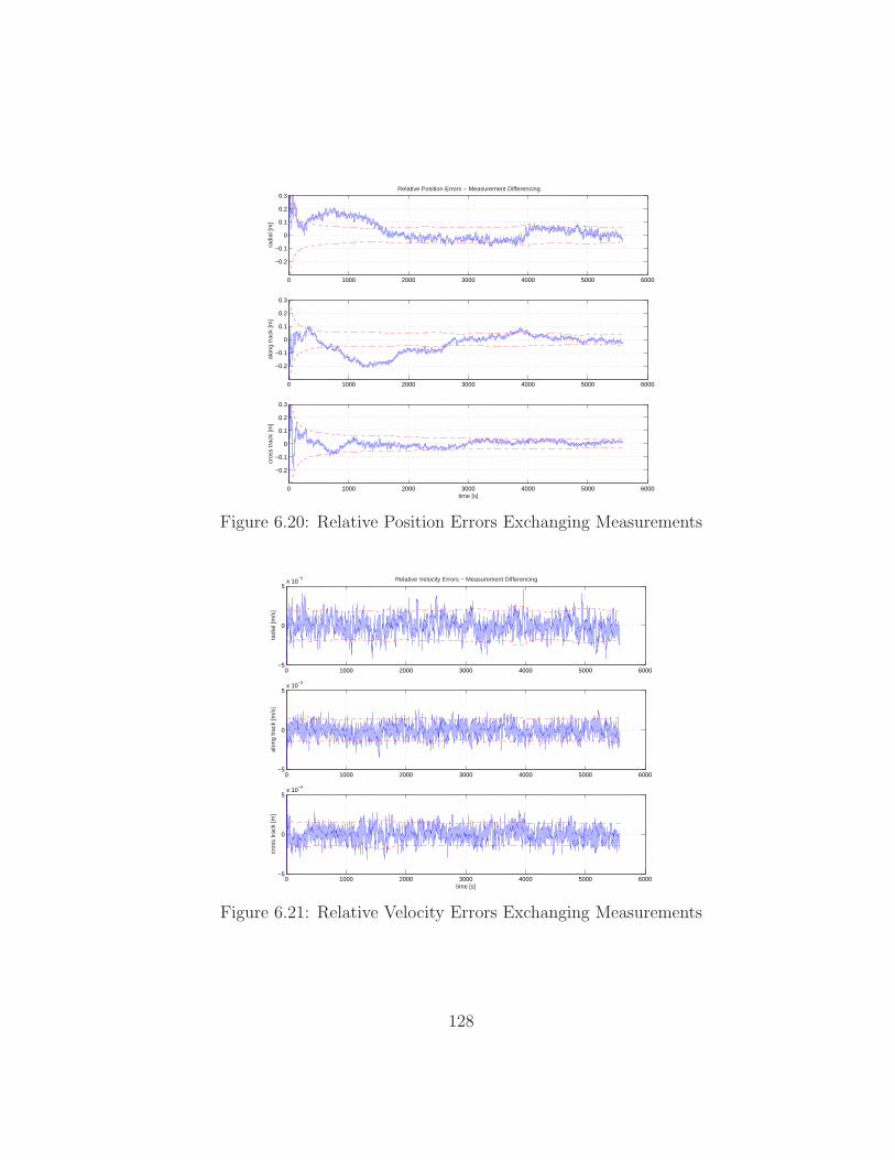
0 1000 2000 3000 4000 5000 6000

−0.2

−0.1

0

0.1

0.2

0.3

radi

al [m

]

Relative Position Errors − Measurement Differencing

0 1000 2000 3000 4000 5000 6000

−0.2

−0.1

0

0.1

0.2

0.3

alon

g tr

ack

[m]

0 1000 2000 3000 4000 5000 6000

−0.2

−0.1

0

0.1

0.2

0.3

time [s]

cros

s tr

ack

[m]

Figure 6.20: Relative Position Errors Exchanging Measurements

0 1000 2000 3000 4000 5000 6000−5

0

5x 10

−3

radi

al [m

/s]

Relative Velocity Errors − Measurement Differencing

0 1000 2000 3000 4000 5000 6000−5

0

5x 10

−3

alon

g tr

ack

[m/s

]

0 1000 2000 3000 4000 5000 6000−5

0

5x 10

−3

time [s]

cros

s tr

ack

[m]

Figure 6.21: Relative Velocity Errors Exchanging Measurements

128

By comparing the results shown in Figures 6.18 and 6.19 with those in

Figures 6.20 and 6.21, it can be seen that the measurement exchange approach

yields approximately an order of magnitude improvement in accuracy over the

state vector exchange approach. Since proximity operations require the highest

accuracy possible, the measurement exchange approach was selected.

The improved accuracy of the relative navigation state obtained using

the measurement exchange approach is achieved by processing single differ-

ence carrier phase measurements. These measurements provide very accurate

information on the relative position of the vehicles since the errors due to

ionospheric delay and GPS SV clock and ephemeris errors are removed in the

single difference process.

In both cases, there was no simulation of data dropouts or data trans-

mission delays. These issues would have to be addressed in the design of an

relative navigation system regardless of which information exchange approach

was chosen.

One benefit of scalar measurement processing used in the GPS/INS

and GPS-only relative navigation filters is that if there are data dropouts due

to communication link problems, the filter would continue to process the local

measurements to improve the absolute navigation state of the local vehicle.

6.2.2 Addition of a Thrust Model in GPS-Only Filter

The dynamics model of the GPS-only filter initially included the effects

of gravity including the J2 effect and atmospheric drag. Any thruster activity

129

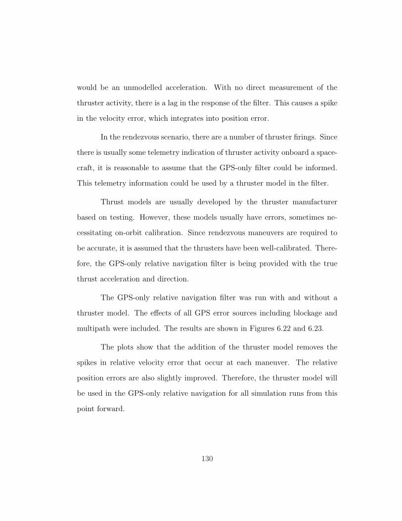
would be an unmodelled acceleration. With no direct measurement of the

thruster activity, there is a lag in the response of the filter. This causes a spike

in the velocity error, which integrates into position error.

In the rendezvous scenario, there are a number of thruster firings. Since

there is usually some telemetry indication of thruster activity onboard a space-

craft, it is reasonable to assume that the GPS-only filter could be informed.

This telemetry information could be used by a thruster model in the filter.

Thrust models are usually developed by the thruster manufacturer

based on testing. However, these models usually have errors, sometimes ne-

cessitating on-orbit calibration. Since rendezvous maneuvers are required to

be accurate, it is assumed that the thrusters have been well-calibrated. There-

fore, the GPS-only relative navigation filter is being provided with the true

thrust acceleration and direction.

The GPS-only relative navigation filter was run with and without a

thruster model. The effects of all GPS error sources including blockage and

multipath were included. The results are shown in Figures 6.22 and 6.23.

The plots show that the addition of the thruster model removes the

spikes in relative velocity error that occur at each maneuver. The relative

position errors are also slightly improved. Therefore, the thruster model will

be used in the GPS-only relative navigation for all simulation runs from this

point forward.

130

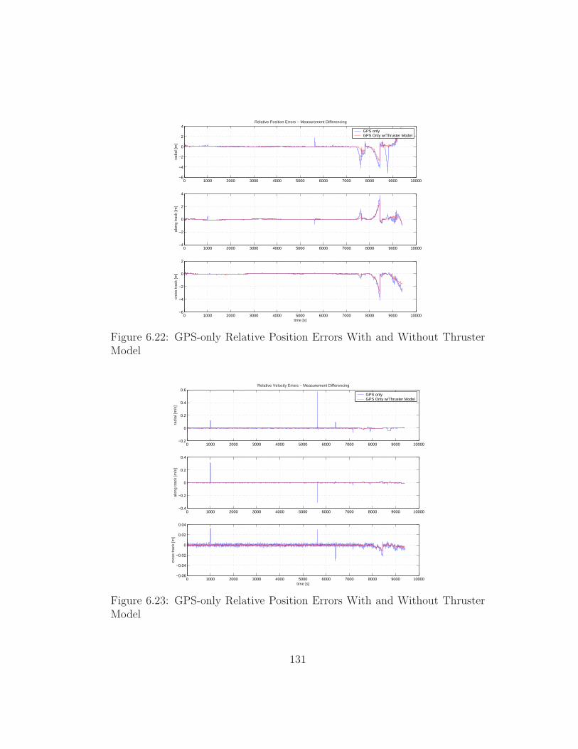
0 1000 2000 3000 4000 5000 6000 7000 8000 9000 10000−6

−4

−2

0

2

4

radi

al [m

]

Relative Position Errors − Measurement Differencing

GPS onlyGPS Only w/Thruster Model

0 1000 2000 3000 4000 5000 6000 7000 8000 9000 10000−4

−2

0

2

4

alon

g tr

ack

[m]

0 1000 2000 3000 4000 5000 6000 7000 8000 9000 10000−6

−4

−2

0

2

time [s]

cros

s tr

ack

[m]

Figure 6.22: GPS-only Relative Position Errors With and Without ThrusterModel

0 1000 2000 3000 4000 5000 6000 7000 8000 9000 10000−0.2

0

0.2

0.4

0.6

radi

al [m

/s]

Relative Velocity Errors − Measurement Differencing

GPS onlyGPS Only w/Thruster Model

0 1000 2000 3000 4000 5000 6000 7000 8000 9000 10000−0.4

−0.2

0

0.2

0.4

alon

g tr

ack

[m/s

]

0 1000 2000 3000 4000 5000 6000 7000 8000 9000 10000−0.06

−0.04

−0.02

0

0.02

0.04

time [s]

cros

s tr

ack

[m]

Figure 6.23: GPS-only Relative Position Errors With and Without ThrusterModel

131

6.2.3 Filter Tuning

The effects of filter tuning on the performance of the relative navigation

filters were studied. The results show that filter tuning has a large effect on

the relative navigation accuracy of both the GPS-only filter and the GPS/INS

filter.

6.2.3.1 GPS-Only Filter Tuning

The GPS-only filter was initially tuned using process noise values that

were used to generate the measurements. The spectral amplitude of the ve-

locity random process was adjusted so that the position and velocity standard

deviations matched the observed absolute position and velocity errors. This

will be referred to as “nominal tuning”.

The GPS-only filter then was tuned to optimize the relative navigation

performance during the final approach, when GPS signals are blocked by the

ISS. The spectral amplitude of the velocity random process was lowered and

noise values for the GPS receiver clock, ionospheric delay, and URE error

states were increased by a factor of ten. This will be referred to as “relative

navigation tuning”.

The process noise covariance values for the GPS-only relative naviga-

tion filter using nominal tuning and relative navigation tuning are presented in

Table 6.5. The value of the process noise correlation coefficient that provided

the best results was ρQ = 0.99, which was used for all GPS-only and GPS/INS

relative navigation filter runs.

132

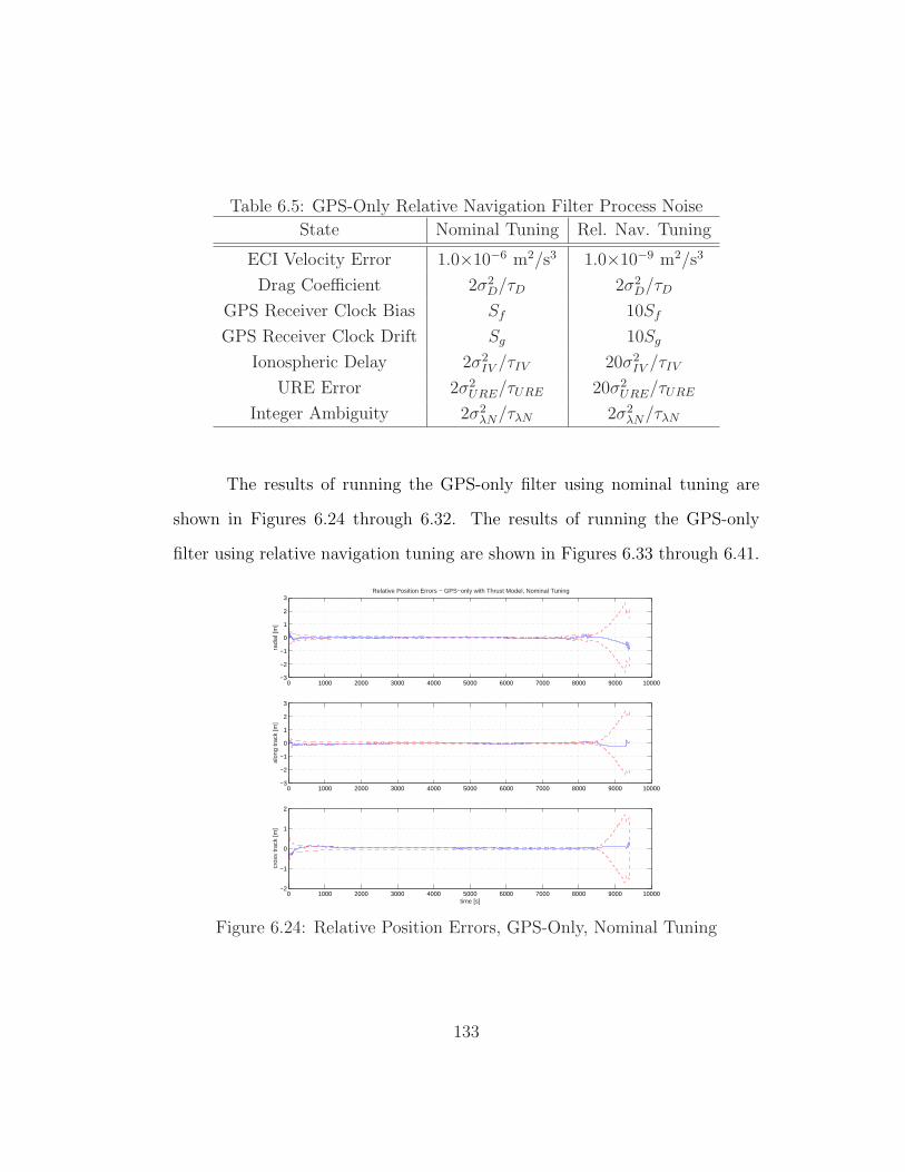
Table 6.5: GPS-Only Relative Navigation Filter Process Noise

State Nominal Tuning Rel. Nav. Tuning

ECI Velocity Error 1.0×10−6 m2/s3 1.0×10−9 m2/s3

Drag Coefficient 2σ2D/τD 2σ2

D/τD

GPS Receiver Clock Bias Sf 10Sf

GPS Receiver Clock Drift Sg 10Sg

Ionospheric Delay 2σ2IV /τIV 20σ2

IV /τIV

URE Error 2σ2URE/τURE 20σ2

URE/τURE

Integer Ambiguity 2σ2λN/τλN 2σ2

λN/τλN

The results of running the GPS-only filter using nominal tuning are

shown in Figures 6.24 through 6.32. The results of running the GPS-only

filter using relative navigation tuning are shown in Figures 6.33 through 6.41.

0 1000 2000 3000 4000 5000 6000 7000 8000 9000 10000−3

−2

−1

0

1

2

3

radi

al [m

]

Relative Position Errors − GPS−only with Thrust Model, Nominal Tuning

0 1000 2000 3000 4000 5000 6000 7000 8000 9000 10000−3

−2

−1

0

1

2

3

alon

g tr

ack

[m]

0 1000 2000 3000 4000 5000 6000 7000 8000 9000 10000−2

−1

0

1

2

time [s]

cros

s tr

ack

[m]

Figure 6.24: Relative Position Errors, GPS-Only, Nominal Tuning

133

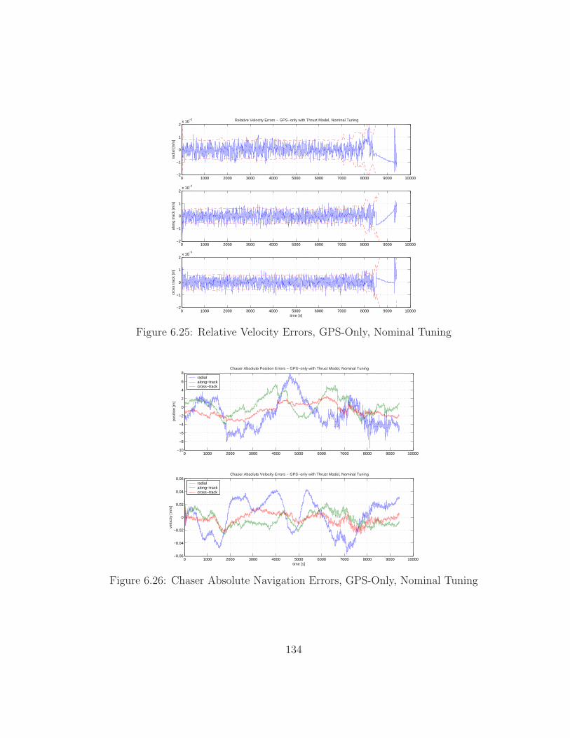
0 1000 2000 3000 4000 5000 6000 7000 8000 9000 10000−2

−1

0

1

2x 10

−3

radi

al [m

/s]

Relative Velocity Errors − GPS−only with Thrust Model, Nominal Tuning

0 1000 2000 3000 4000 5000 6000 7000 8000 9000 10000−2

−1

0

1

2x 10

−3

alon

g tr

ack

[m/s

]

0 1000 2000 3000 4000 5000 6000 7000 8000 9000 10000−2

−1

0

1

2x 10

−3

time [s]

cros

s tr

ack

[m]

Figure 6.25: Relative Velocity Errors, GPS-Only, Nominal Tuning

0 1000 2000 3000 4000 5000 6000 7000 8000 9000 10000−10

−8

−6

−4

−2

0

2

4

6

8

posi

tion

[m]

Chaser Absolute Position Errors − GPS−only with Thrust Model, Nominal Tuning


0 1000 2000 3000 4000 5000 6000 7000 8000 9000 10000−0.06

−0.04

−0.02

0

0.02

0.04

0.06

time [s]

velo

city

[m/s

]

Chaser Absolute Velocity Errors − GPS−only with Thrust Model, Nominal Tuning


Figure 6.26: Chaser Absolute Navigation Errors, GPS-Only, Nominal Tuning

134

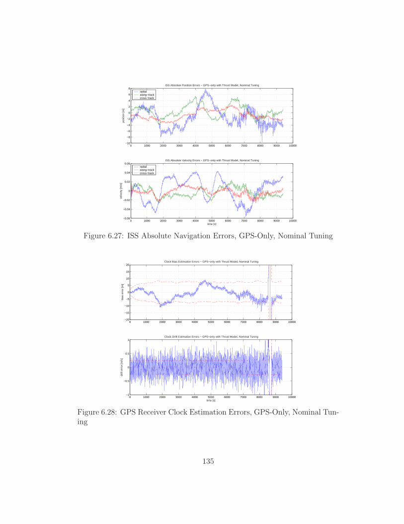
0 1000 2000 3000 4000 5000 6000 7000 8000 9000 10000−10

−8

−6

−4

−2

0

2

4

6

8

posi

tion

[m]

ISS Absolute Position Errors − GPS−only with Thrust Model, Nominal Tuning


0 1000 2000 3000 4000 5000 6000 7000 8000 9000 10000−0.06

−0.04

−0.02

0

0.02

0.04

0.06

time [s]

velo

city

[m/s

]

ISS Absolute Velocity Errors − GPS−only with Thrust Model, Nominal Tuning


Figure 6.27: ISS Absolute Navigation Errors, GPS-Only, Nominal Tuning

0 1000 2000 3000 4000 5000 6000 7000 8000 9000 10000−20

−15

−10

−5

0

5

10

15

20

bias

err

or [m

]

Clock Bias Estimation Errors − GPS−only with Thrust Model, Nominal Tuning

0 1000 2000 3000 4000 5000 6000 7000 8000 9000 10000−1

−0.5

0

0.5

1

time [s]

drift

err

or [m

/s]

Clock Drift Estimation Errors − GPS−only with Thrust Model, Nominal Tuning

Figure 6.28: GPS Receiver Clock Estimation Errors, GPS-Only, Nominal Tun-ing

135

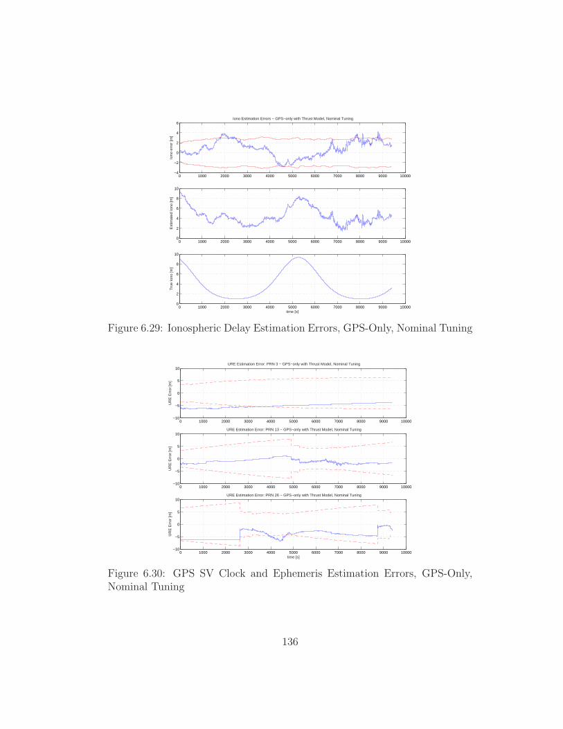
0 1000 2000 3000 4000 5000 6000 7000 8000 9000 10000−4

−2

0

2

4

6

Iono

err

or [m

]

Iono Estimation Errors − GPS−only with Thrust Model, Nominal Tuning

0 1000 2000 3000 4000 5000 6000 7000 8000 9000 100000

2

4

6

8

10

Est

imat

ed Io

no [m

]

0 1000 2000 3000 4000 5000 6000 7000 8000 9000 100000

2

4

6

8

10

time [s]

Tru

e Io

no [m

]

Figure 6.29: Ionospheric Delay Estimation Errors, GPS-Only, Nominal Tuning

0 1000 2000 3000 4000 5000 6000 7000 8000 9000 10000−10

−5

0

5

10

UR

E E

rror

[m]

URE Estimation Error: PRN 3 − GPS−only with Thrust Model, Nominal Tuning

0 1000 2000 3000 4000 5000 6000 7000 8000 9000 10000−10

−5

0

5

10

UR

E E

rror

[m]


0 1000 2000 3000 4000 5000 6000 7000 8000 9000 10000−10

−5

0

5

10

time [s]

UR

E E

rror

[m]


Figure 6.30: GPS SV Clock and Ephemeris Estimation Errors, GPS-Only,Nominal Tuning

136

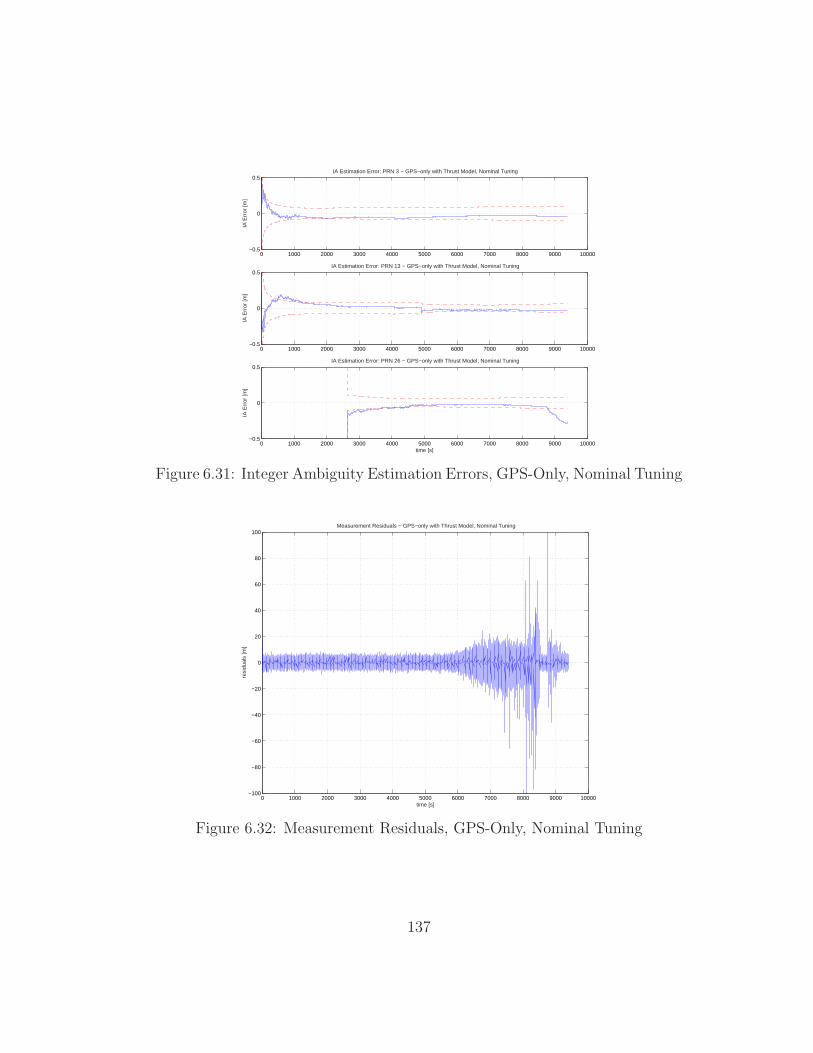
0 1000 2000 3000 4000 5000 6000 7000 8000 9000 10000−0.5

0

0.5

IA E

rror

[m]

IA Estimation Error: PRN 3 − GPS−only with Thrust Model, Nominal Tuning

0 1000 2000 3000 4000 5000 6000 7000 8000 9000 10000−0.5

0

0.5

IA E

rror

[m]


0 1000 2000 3000 4000 5000 6000 7000 8000 9000 10000−0.5

0

0.5

time [s]

IA E

rror

[m]


Figure 6.31: Integer Ambiguity Estimation Errors, GPS-Only, Nominal Tuning

0 1000 2000 3000 4000 5000 6000 7000 8000 9000 10000−100

−80

−60

−40

−20

0

20

40

60

80

100

time [s]

resi

dual

s [m

]

Measurement Residuals − GPS−only with Thrust Model, Nominal Tuning

Figure 6.32: Measurement Residuals, GPS-Only, Nominal Tuning

137

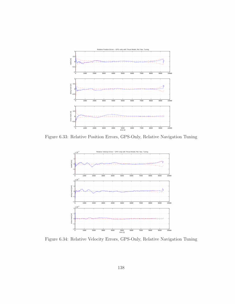
0 1000 2000 3000 4000 5000 6000 7000 8000 9000 10000−1

−0.5

0

0.5

1

radi

al [m

]

Relative Position Errors − GPS−only with Thrust Model, Rel. Nav. Tuning

0 1000 2000 3000 4000 5000 6000 7000 8000 9000 10000−1

−0.5

0

0.5

1

alon

g tr

ack

[m]

0 1000 2000 3000 4000 5000 6000 7000 8000 9000 10000−1

−0.5

0

0.5

1

time [s]

cros

s tr

ack

[m]

Figure 6.33: Relative Position Errors, GPS-Only, Relative Navigation Tuning

0 1000 2000 3000 4000 5000 6000 7000 8000 9000 10000−2

−1

0

1

2x 10

−3

radi

al [m

/s]

Relative Velocity Errors − GPS−only with Thrust Model, Rel. Nav. Tuning

0 1000 2000 3000 4000 5000 6000 7000 8000 9000 10000−2

−1

0

1

2x 10

−3

alon

g tr

ack

[m/s

]

0 1000 2000 3000 4000 5000 6000 7000 8000 9000 10000−2

−1

0

1

2x 10

−3

time [s]

cros

s tr

ack

[m]

Figure 6.34: Relative Velocity Errors, GPS-Only, Relative Navigation Tuning

138

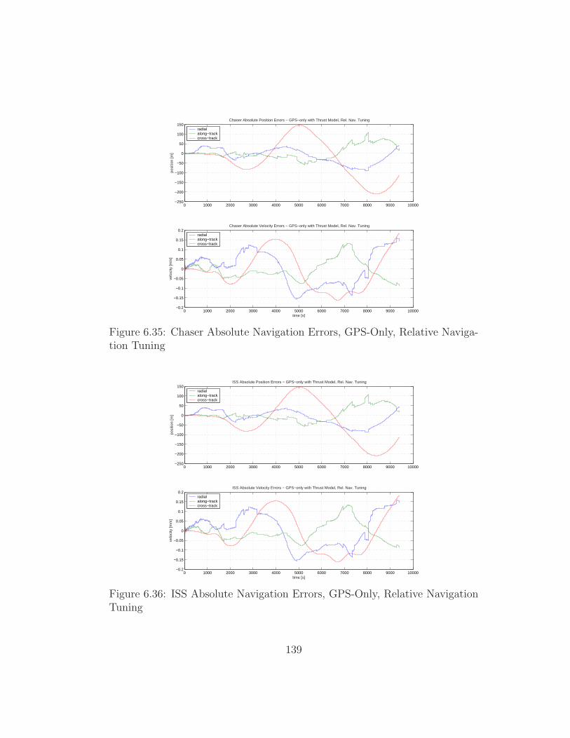
0 1000 2000 3000 4000 5000 6000 7000 8000 9000 10000−250

−200

−150

−100

−50

0

50

100

150

posi

tion

[m]

Chaser Absolute Position Errors − GPS−only with Thrust Model, Rel. Nav. Tuning


0 1000 2000 3000 4000 5000 6000 7000 8000 9000 10000−0.2

−0.15

−0.1

−0.05

0

0.05

0.1

0.15

0.2

time [s]

velo

city

[m/s

]

Chaser Absolute Velocity Errors − GPS−only with Thrust Model, Rel. Nav. Tuning


Figure 6.35: Chaser Absolute Navigation Errors, GPS-Only, Relative Naviga-tion Tuning

0 1000 2000 3000 4000 5000 6000 7000 8000 9000 10000−250

−200

−150

−100

−50

0

50

100

150

posi

tion

[m]

ISS Absolute Position Errors − GPS−only with Thrust Model, Rel. Nav. Tuning


0 1000 2000 3000 4000 5000 6000 7000 8000 9000 10000−0.2

−0.15

−0.1

−0.05

0

0.05

0.1

0.15

0.2

time [s]

velo

city

[m/s

]

ISS Absolute Velocity Errors − GPS−only with Thrust Model, Rel. Nav. Tuning


Figure 6.36: ISS Absolute Navigation Errors, GPS-Only, Relative NavigationTuning

139

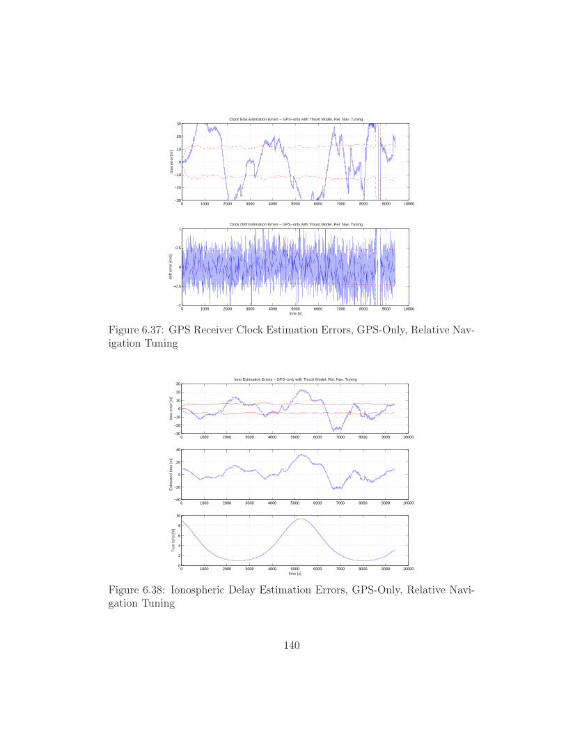
0 1000 2000 3000 4000 5000 6000 7000 8000 9000 10000−30

−20

−10

0

10

20

30

bias

err

or [m

]

Clock Bias Estimation Errors − GPS−only with Thrust Model, Rel. Nav. Tuning

0 1000 2000 3000 4000 5000 6000 7000 8000 9000 10000−1

−0.5

0

0.5

1

time [s]

drift

err

or [m

/s]

Clock Drift Estimation Errors − GPS−only with Thrust Model, Rel. Nav. Tuning

Figure 6.37: GPS Receiver Clock Estimation Errors, GPS-Only, Relative Nav-igation Tuning

0 1000 2000 3000 4000 5000 6000 7000 8000 9000 10000−30

−20

−10

0

10

20

30

Iono

err

or [m

]

Iono Estimation Errors − GPS−only with Thrust Model, Rel. Nav. Tuning

0 1000 2000 3000 4000 5000 6000 7000 8000 9000 10000−40

−20

0

20

40

Est

imat

ed Io

no [m

]

0 1000 2000 3000 4000 5000 6000 7000 8000 9000 100000

2

4

6

8

10

time [s]

Tru

e Io

no [m

]

Figure 6.38: Ionospheric Delay Estimation Errors, GPS-Only, Relative Navi-gation Tuning

140

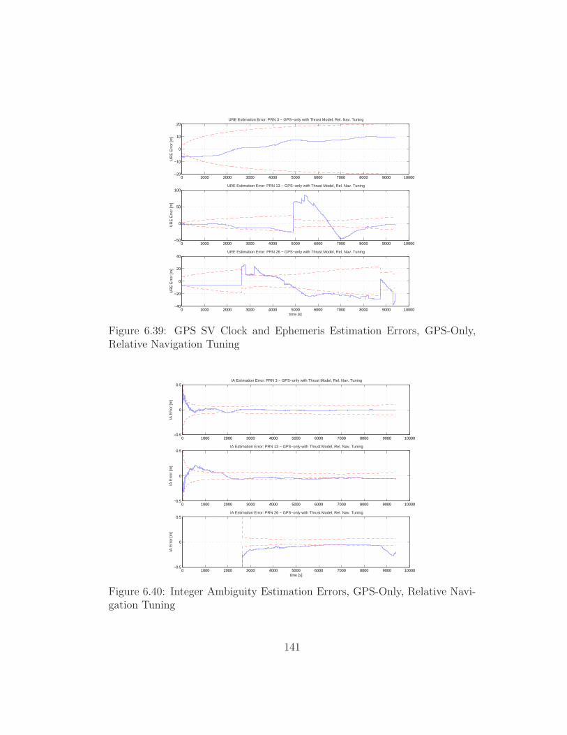
0 1000 2000 3000 4000 5000 6000 7000 8000 9000 10000−20

−10

0

10

20

UR

E E

rror

[m]

URE Estimation Error: PRN 3 − GPS−only with Thrust Model, Rel. Nav. Tuning

0 1000 2000 3000 4000 5000 6000 7000 8000 9000 10000−50

0

50

100

UR

E E

rror

[m]


0 1000 2000 3000 4000 5000 6000 7000 8000 9000 10000−40

−20

0

20

40

time [s]

UR

E E

rror

[m]


Figure 6.39: GPS SV Clock and Ephemeris Estimation Errors, GPS-Only,Relative Navigation Tuning

0 1000 2000 3000 4000 5000 6000 7000 8000 9000 10000−0.5

0

0.5

IA E

rror

[m]

IA Estimation Error: PRN 3 − GPS−only with Thrust Model, Rel. Nav. Tuning

0 1000 2000 3000 4000 5000 6000 7000 8000 9000 10000−0.5

0

0.5

IA E

rror

[m]


0 1000 2000 3000 4000 5000 6000 7000 8000 9000 10000−0.5

0

0.5

time [s]

IA E

rror

[m]


Figure 6.40: Integer Ambiguity Estimation Errors, GPS-Only, Relative Navi-gation Tuning

141

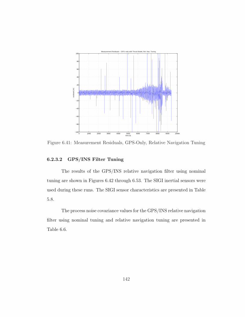
0 1000 2000 3000 4000 5000 6000 7000 8000 9000 10000−100

−80

−60

−40

−20

0

20

40

60

80

100

time [s]

resi

dual

s [m

]

Measurement Residuals − GPS−only with Thrust Model, Rel. Nav. Tuning

Figure 6.41: Measurement Residuals, GPS-Only, Relative Navigation Tuning

6.2.3.2 GPS/INS Filter Tuning

The results of the GPS/INS relative navigation filter using nominal

tuning are shown in Figures 6.42 through 6.53. The SIGI inertial sensors were

used during these runs. The SIGI sensor characteristics are presented in Table

5.8.

The process noise covariance values for the GPS/INS relative navigation

filter using nominal tuning and relative navigation tuning are presented in

Table 6.6.

142

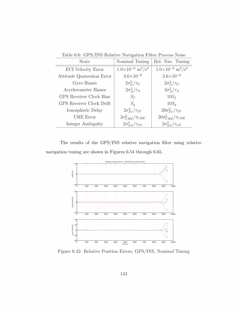
Table 6.6: GPS/INS Relative Navigation Filter Process Noise

State Nominal Tuning Rel. Nav. Tuning

ECI Velocity Error 1.0×10−6 m2/s3 1.0×10−9 m2/s3

Attitude Quaternion Error 3.6×10−6 3.6×10−6

Gyro Biases 2σ2G/τG 2σ2

G/τG

Accelerometer Biases 2σ2A/τA 2σ2

A/τA

GPS Receiver Clock Bias Sf 10Sf

GPS Receiver Clock Drift Sg 10Sg

Ionospheric Delay 2σ2IV /τIV 20σ2

IV /τIV

URE Error 2σ2URE/τURE 20σ2

URE/τURE

Integer Ambiguity 2σ2λN/τλN 2σ2

λN/τλN

The results of the GPS/INS relative navigation filter using relative

navigation tuning are shown in Figures 6.54 through 6.65.

0 1000 2000 3000 4000 5000 6000 7000 8000 9000 10000−50

0

50

radi

al [m

]

Relative Position Errors − GPS/INS with SIGI Sensors

0 1000 2000 3000 4000 5000 6000 7000 8000 9000 10000−50

0

50

alon

g tr

ack

[m]

0 1000 2000 3000 4000 5000 6000 7000 8000 9000 10000−40

−20

0

20

40

time [s]

cros

s tr

ack

[m]

Figure 6.42: Relative Position Errors, GPS/INS, Nominal Tuning

143

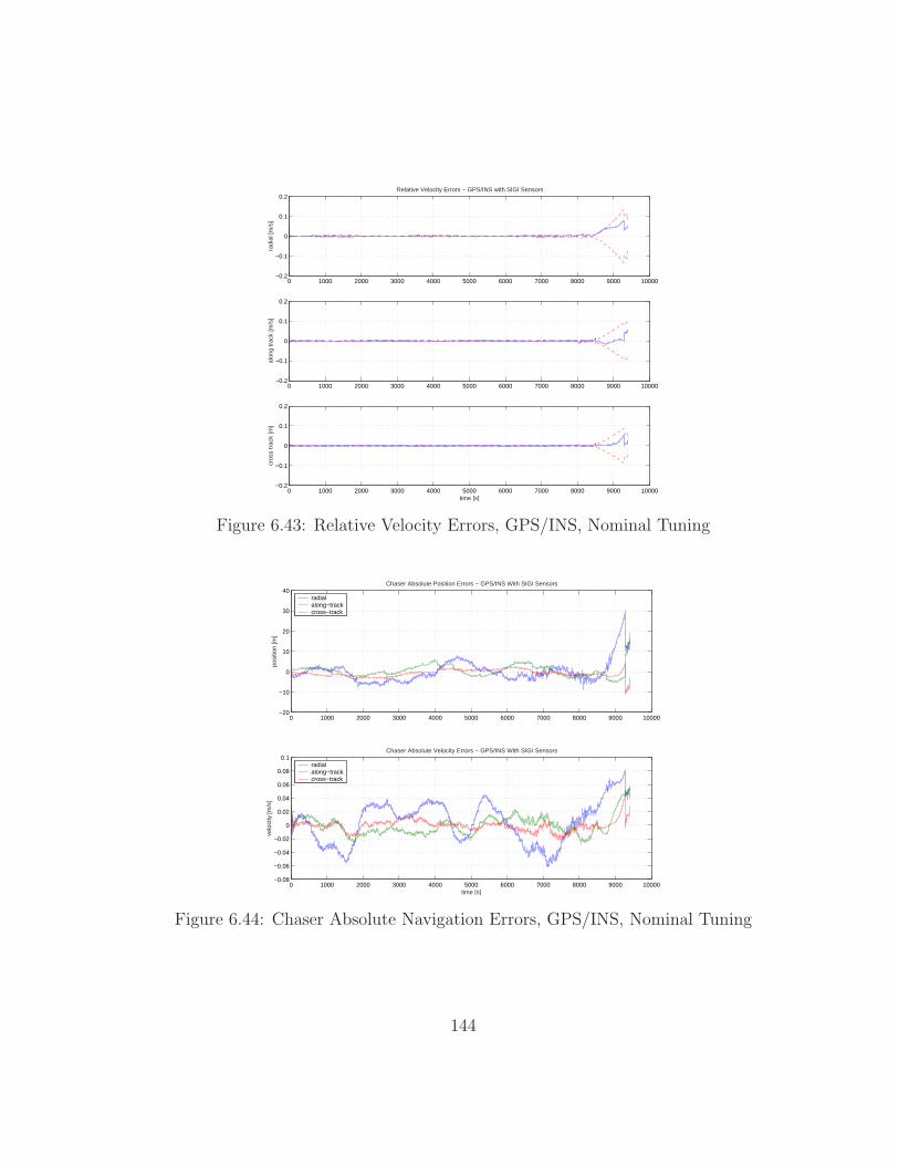
0 1000 2000 3000 4000 5000 6000 7000 8000 9000 10000−0.2

−0.1

0

0.1

0.2

radi

al [m

/s]

Relative Velocity Errors − GPS/INS with SIGI Sensors

0 1000 2000 3000 4000 5000 6000 7000 8000 9000 10000−0.2

−0.1

0

0.1

0.2

alon

g tr

ack

[m/s

]

0 1000 2000 3000 4000 5000 6000 7000 8000 9000 10000−0.2

−0.1

0

0.1

0.2

time [s]

cros

s tr

ack

[m]

Figure 6.43: Relative Velocity Errors, GPS/INS, Nominal Tuning

0 1000 2000 3000 4000 5000 6000 7000 8000 9000 10000−20

−10

0

10

20

30

40

posi

tion

[m]



0 1000 2000 3000 4000 5000 6000 7000 8000 9000 10000−0.08

−0.06

−0.04

−0.02

0

0.02

0.04

0.06

0.08

0.1

time [s]

velo

city

[m/s

]



Figure 6.44: Chaser Absolute Navigation Errors, GPS/INS, Nominal Tuning

144

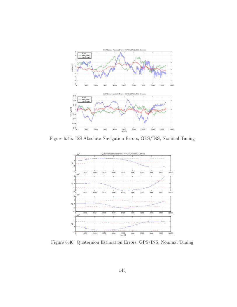
0 1000 2000 3000 4000 5000 6000 7000 8000 9000 10000−10

−8

−6

−4

−2

0

2

4

6

8

posi

tion

[m]

ISS Absolute Position Errors − GPS/INS With SIGI Sensors


0 1000 2000 3000 4000 5000 6000 7000 8000 9000 10000−0.08

−0.06

−0.04

−0.02

0

0.02

0.04

0.06

time [s]

velo

city

[m/s

]

ISS Absolute Velocity Errors − GPS/INS With SIGI Sensors


Figure 6.45: ISS Absolute Navigation Errors, GPS/INS, Nominal Tuning

0 1000 2000 3000 4000 5000 6000 7000 8000 9000 10000−4

−2

0

2x 10

−3

q1


0 1000 2000 3000 4000 5000 6000 7000 8000 9000 10000−2

−1

0

1

2x 10

−3

q2

0 1000 2000 3000 4000 5000 6000 7000 8000 9000 10000−2

−1

0

1

2x 10

−3

q3

0 1000 2000 3000 4000 5000 6000 7000 8000 9000 10000−1

0

1

2x 10

−3

time [s]

q4

Figure 6.46: Quaternion Estimation Errors, GPS/INS, Nominal Tuning

145

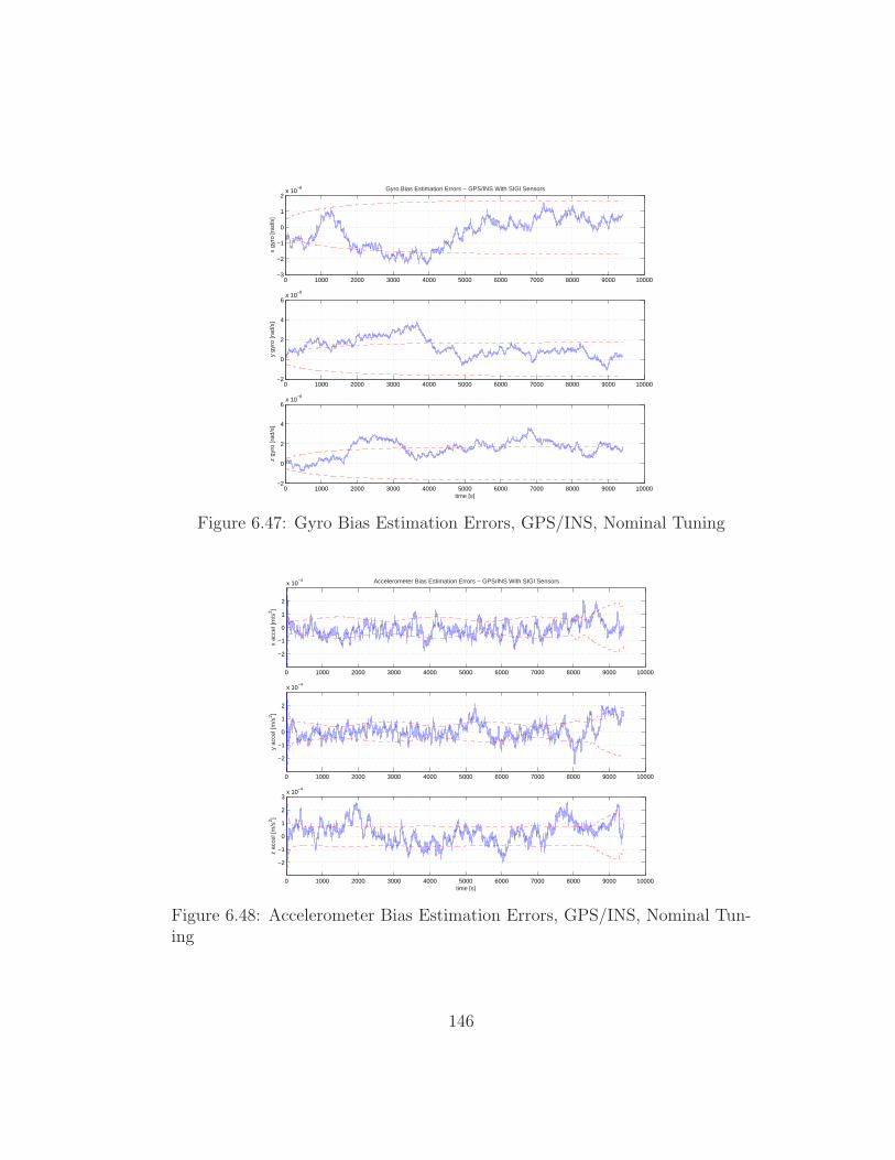
0 1000 2000 3000 4000 5000 6000 7000 8000 9000 10000−3

−2

−1

0

1

2x 10

−8

x gy

ro [r

ad/s

]


0 1000 2000 3000 4000 5000 6000 7000 8000 9000 10000−2

0

2

4

6x 10

−8

y gy

ro [r

ad/s

]

0 1000 2000 3000 4000 5000 6000 7000 8000 9000 10000−2

0

2

4

6x 10

−8

time [s]

z gy

ro [r

ad/s

]

Figure 6.47: Gyro Bias Estimation Errors, GPS/INS, Nominal Tuning

0 1000 2000 3000 4000 5000 6000 7000 8000 9000 10000

−2

−1

0

1

2

x 10−4

x ac

cel [

m/s

2 ]


0 1000 2000 3000 4000 5000 6000 7000 8000 9000 10000

−2

−1

0

1

2

x 10−4

y ac

cel [

m/s

2 ]

0 1000 2000 3000 4000 5000 6000 7000 8000 9000 10000

−2

−1

0

1

2

3x 10

−4

time [s]

z ac

cel [

m/s

2 ]

Figure 6.48: Accelerometer Bias Estimation Errors, GPS/INS, Nominal Tun-ing

146

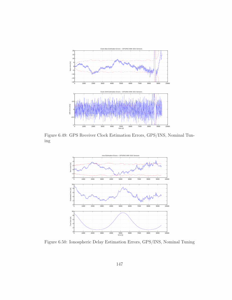
0 1000 2000 3000 4000 5000 6000 7000 8000 9000 10000−20

−15

−10

−5

0

5

10

15

20

bias

err

or [m

]


0 1000 2000 3000 4000 5000 6000 7000 8000 9000 10000−1

−0.5

0

0.5

1

time [s]

drift

err

or [m

/s]


Figure 6.49: GPS Receiver Clock Estimation Errors, GPS/INS, Nominal Tun-ing

0 1000 2000 3000 4000 5000 6000 7000 8000 9000 10000−4

−2

0

2

4

6

Iono

err

or [m

]


0 1000 2000 3000 4000 5000 6000 7000 8000 9000 100000

2

4

6

8

10

Est

imat

ed Io

no [m

]

0 1000 2000 3000 4000 5000 6000 7000 8000 9000 100000

2

4

6

8

10

time [s]

Tru

e Io

no [m

]

Figure 6.50: Ionospheric Delay Estimation Errors, GPS/INS, Nominal Tuning

147

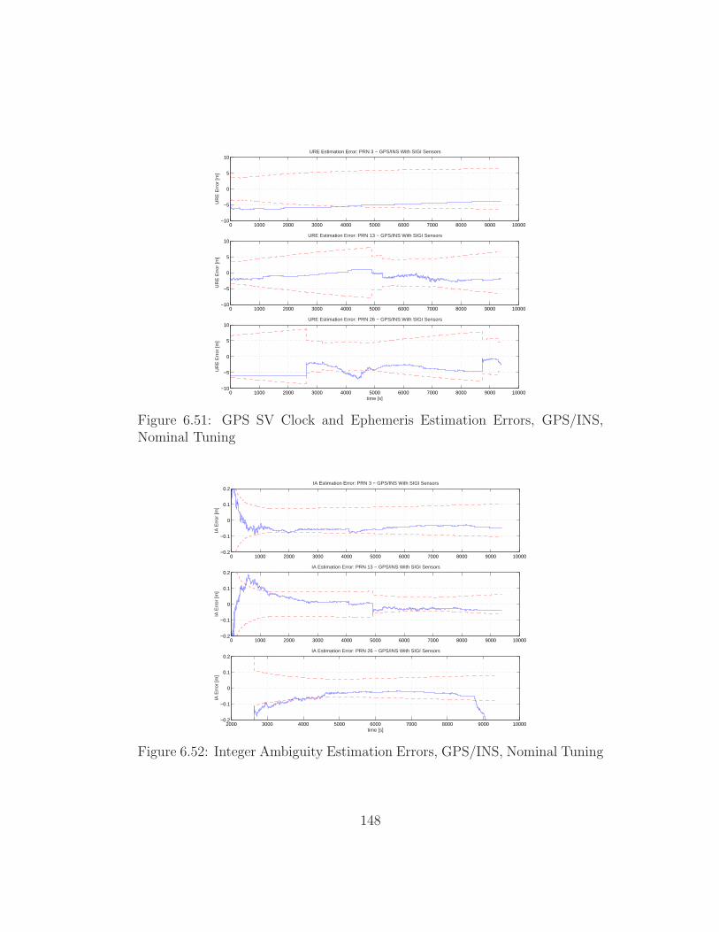
0 1000 2000 3000 4000 5000 6000 7000 8000 9000 10000−10

−5

0

5

10

UR

E E

rror

[m]


0 1000 2000 3000 4000 5000 6000 7000 8000 9000 10000−10

−5

0

5

10

UR

E E

rror

[m]


0 1000 2000 3000 4000 5000 6000 7000 8000 9000 10000−10

−5

0

5

10

time [s]

UR

E E

rror

[m]


Figure 6.51: GPS SV Clock and Ephemeris Estimation Errors, GPS/INS,Nominal Tuning

0 1000 2000 3000 4000 5000 6000 7000 8000 9000 10000−0.2

−0.1

0

0.1

0.2

IA E

rror

[m]

IA Estimation Error: PRN 3 − GPS/INS With SIGI Sensors

0 1000 2000 3000 4000 5000 6000 7000 8000 9000 10000−0.2

−0.1

0

0.1

0.2

IA E

rror

[m]


2000 3000 4000 5000 6000 7000 8000 9000 10000−0.2

−0.1

0

0.1

0.2

time [s]

IA E

rror

[m]


Figure 6.52: Integer Ambiguity Estimation Errors, GPS/INS, Nominal Tuning

148

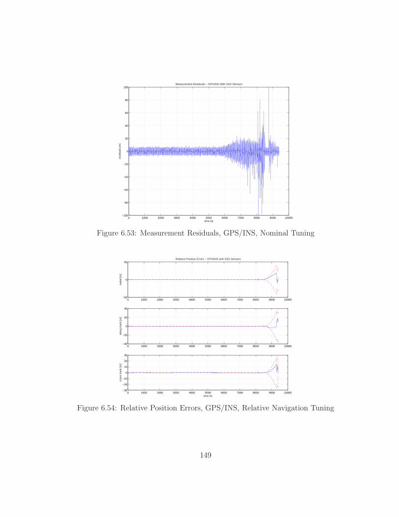
0 1000 2000 3000 4000 5000 6000 7000 8000 9000 10000−100

−80

−60

−40

−20

0

20

40

60

80

100

time [s]

resi

dual

s [m

]


Figure 6.53: Measurement Residuals, GPS/INS, Nominal Tuning

0 1000 2000 3000 4000 5000 6000 7000 8000 9000 10000−50

0

50

radi

al [m

]

Relative Position Errors − GPS/INS with SIGI Sensors

0 1000 2000 3000 4000 5000 6000 7000 8000 9000 10000−40

−20

0

20

40

alon

g tr

ack

[m]

0 1000 2000 3000 4000 5000 6000 7000 8000 9000 10000−30

−20

−10

0

10

20

30

time [s]

cros

s tr

ack

[m]

Figure 6.54: Relative Position Errors, GPS/INS, Relative Navigation Tuning

149

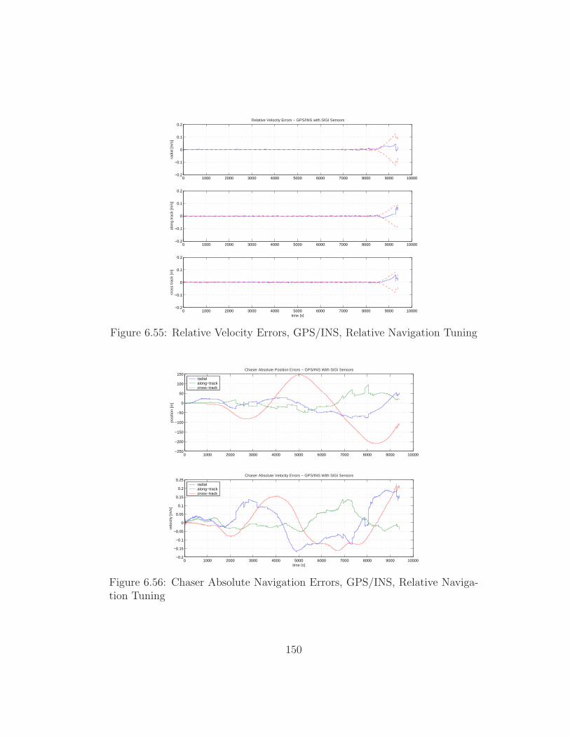
0 1000 2000 3000 4000 5000 6000 7000 8000 9000 10000−0.2

−0.1

0

0.1

0.2

radi

al [m

/s]

Relative Velocity Errors − GPS/INS with SIGI Sensors

0 1000 2000 3000 4000 5000 6000 7000 8000 9000 10000−0.2

−0.1

0

0.1

0.2

alon

g tr

ack

[m/s

]

0 1000 2000 3000 4000 5000 6000 7000 8000 9000 10000−0.2

−0.1

0

0.1

0.2

time [s]

cros

s tr

ack

[m]

Figure 6.55: Relative Velocity Errors, GPS/INS, Relative Navigation Tuning

0 1000 2000 3000 4000 5000 6000 7000 8000 9000 10000−250

−200

−150

−100

−50

0

50

100

150

posi

tion

[m]



0 1000 2000 3000 4000 5000 6000 7000 8000 9000 10000−0.2

−0.15

−0.1

−0.05

0

0.05

0.1

0.15

0.2

0.25

time [s]

velo

city

[m/s

]



Figure 6.56: Chaser Absolute Navigation Errors, GPS/INS, Relative Naviga-tion Tuning

150

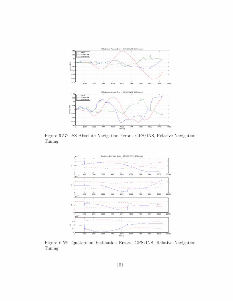
0 1000 2000 3000 4000 5000 6000 7000 8000 9000 10000−250

−200

−150

−100

−50

0

50

100

150

posi

tion

[m]

ISS Absolute Position Errors − GPS/INS With SIGI Sensors


0 1000 2000 3000 4000 5000 6000 7000 8000 9000 10000−0.2

−0.15

−0.1

−0.05

0

0.05

0.1

0.15

0.2

time [s]

velo

city

[m/s

]

ISS Absolute Velocity Errors − GPS/INS With SIGI Sensors


Figure 6.57: ISS Absolute Navigation Errors, GPS/INS, Relative NavigationTuning

0 1000 2000 3000 4000 5000 6000 7000 8000 9000 10000−2

−1

0

1

2x 10

−3

q1


0 1000 2000 3000 4000 5000 6000 7000 8000 9000 10000−2

−1

0

1

2x 10

−3

q2

0 1000 2000 3000 4000 5000 6000 7000 8000 9000 10000−2

−1

0

1

2x 10

−3

q3

0 1000 2000 3000 4000 5000 6000 7000 8000 9000 10000−1

−0.5

0

0.5

1x 10

−3

time [s]

q4

Figure 6.58: Quaternion Estimation Errors, GPS/INS, Relative NavigationTuning

151

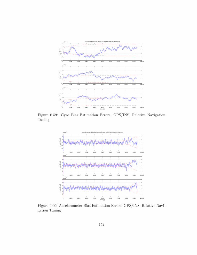
0 1000 2000 3000 4000 5000 6000 7000 8000 9000 10000−3

−2

−1

0

1

2x 10

−8

x gy

ro [r

ad/s

]


0 1000 2000 3000 4000 5000 6000 7000 8000 9000 10000−2

0

2

4

6x 10

−8

y gy

ro [r

ad/s

]

0 1000 2000 3000 4000 5000 6000 7000 8000 9000 10000−2

0

2

4

6x 10

−8

time [s]

z gy

ro [r

ad/s

]

Figure 6.59: Gyro Bias Estimation Errors, GPS/INS, Relative NavigationTuning

0 1000 2000 3000 4000 5000 6000 7000 8000 9000 10000

−2

−1

0

1

2

x 10−4

x ac

cel [

m/s

2 ]


0 1000 2000 3000 4000 5000 6000 7000 8000 9000 10000

−2

−1

0

1

2

x 10−4

y ac

cel [

m/s

2 ]

0 1000 2000 3000 4000 5000 6000 7000 8000 9000 10000

−2

−1

0

1

2

3x 10

−4

time [s]

z ac

cel [

m/s

2 ]

Figure 6.60: Accelerometer Bias Estimation Errors, GPS/INS, Relative Navi-gation Tuning

152

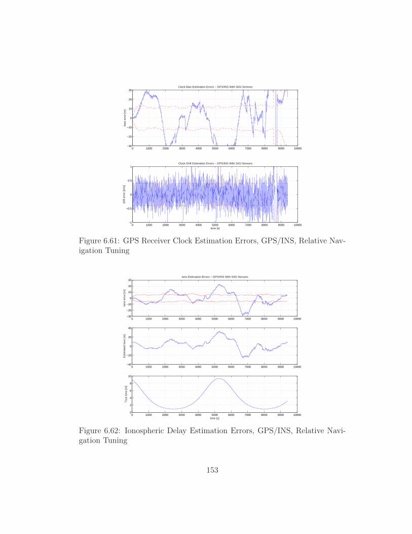
0 1000 2000 3000 4000 5000 6000 7000 8000 9000 10000−30

−20

−10

0

10

20

30

bias

err

or [m

]


0 1000 2000 3000 4000 5000 6000 7000 8000 9000 10000−1

−0.5

0

0.5

1

time [s]

drift

err

or [m

/s]


Figure 6.61: GPS Receiver Clock Estimation Errors, GPS/INS, Relative Nav-igation Tuning

0 1000 2000 3000 4000 5000 6000 7000 8000 9000 10000−30

−20

−10

0

10

20

30

Iono

err

or [m

]


0 1000 2000 3000 4000 5000 6000 7000 8000 9000 10000−40

−20

0

20

40

Est

imat

ed Io

no [m

]

0 1000 2000 3000 4000 5000 6000 7000 8000 9000 100000

2

4

6

8

10

time [s]

Tru

e Io

no [m

]

Figure 6.62: Ionospheric Delay Estimation Errors, GPS/INS, Relative Navi-gation Tuning

153

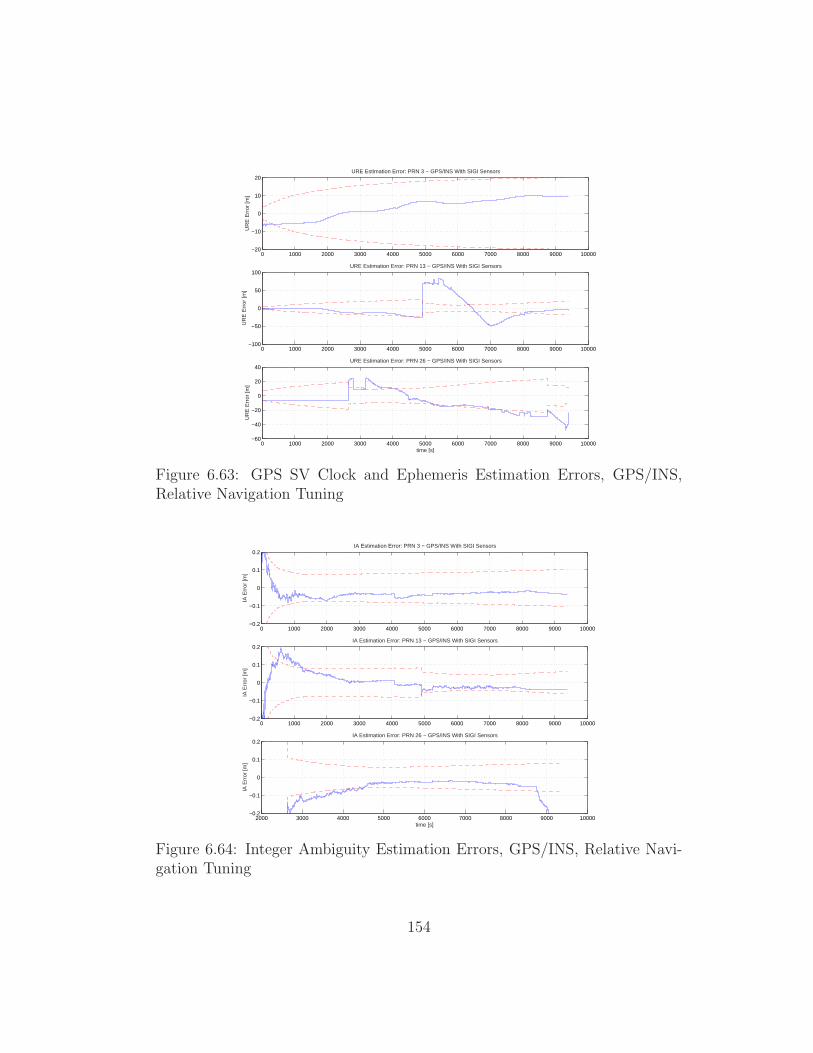
0 1000 2000 3000 4000 5000 6000 7000 8000 9000 10000−20

−10

0

10

20

UR

E E

rror

[m]


0 1000 2000 3000 4000 5000 6000 7000 8000 9000 10000−100

−50

0

50

100

UR

E E

rror

[m]


0 1000 2000 3000 4000 5000 6000 7000 8000 9000 10000−60

−40

−20

0

20

40

time [s]

UR

E E

rror

[m]


Figure 6.63: GPS SV Clock and Ephemeris Estimation Errors, GPS/INS,Relative Navigation Tuning

0 1000 2000 3000 4000 5000 6000 7000 8000 9000 10000−0.2

−0.1

0

0.1

0.2

IA E

rror

[m]


0 1000 2000 3000 4000 5000 6000 7000 8000 9000 10000−0.2

−0.1

0

0.1

0.2

IA E

rror

[m]


2000 3000 4000 5000 6000 7000 8000 9000 10000−0.2

−0.1

0

0.1

0.2

time [s]

IA E

rror

[m]


Figure 6.64: Integer Ambiguity Estimation Errors, GPS/INS, Relative Navi-gation Tuning

154

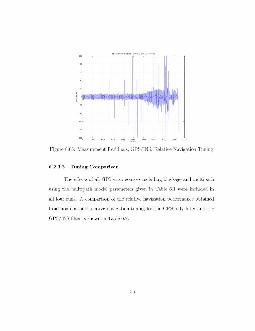
0 1000 2000 3000 4000 5000 6000 7000 8000 9000 10000−100

−80

−60

−40

−20

0

20

40

60

80

100

time [s]

resi

dual

s [m

]


Figure 6.65: Measurement Residuals, GPS/INS, Relative Navigation Tuning

6.2.3.3 Tuning Comparison

The effects of all GPS error sources including blockage and multipath

using the multipath model parameters given in Table 6.1 were included in

all four runs. A comparison of the relative navigation performance obtained

from nominal and relative navigation tuning for the GPS-only filter and the

GPS/INS filter is shown in Table 6.7.

155

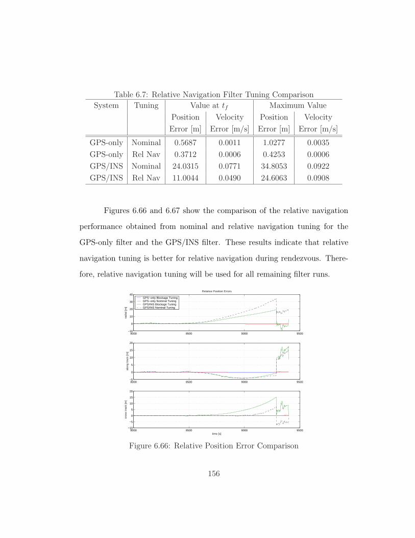
Table 6.7: Relative Navigation Filter Tuning Comparison

System Tuning Value at tf Maximum Value



GPS-only Nominal 0.5687 0.0011 1.0277 0.0035

GPS-only Rel Nav 0.3712 0.0006 0.4253 0.0006

GPS/INS Nominal 24.0315 0.0771 34.8053 0.0922

GPS/INS Rel Nav 11.0044 0.0490 24.6063 0.0908

Figures 6.66 and 6.67 show the comparison of the relative navigation

performance obtained from nominal and relative navigation tuning for the

GPS-only filter and the GPS/INS filter. These results indicate that relative

navigation tuning is better for relative navigation during rendezvous. There-

fore, relative navigation tuning will be used for all remaining filter runs.

8000 8500 9000 9500−10

0

10

20

30

40

radi

al [m

]

Relative Position Errors

GPS−only Blockage TuningGPS−only Nominal TuningGPS/INS Blockage TuningGPS/INS Nominal Tuning

8000 8500 9000 9500−5

0

5

10

15

20

alon

g tr

ack

[m]

8000 8500 9000 9500−10

−5

0

5

10

15

20

time [s]

cros

s tr

ack

[m]

Figure 6.66: Relative Position Error Comparison

156

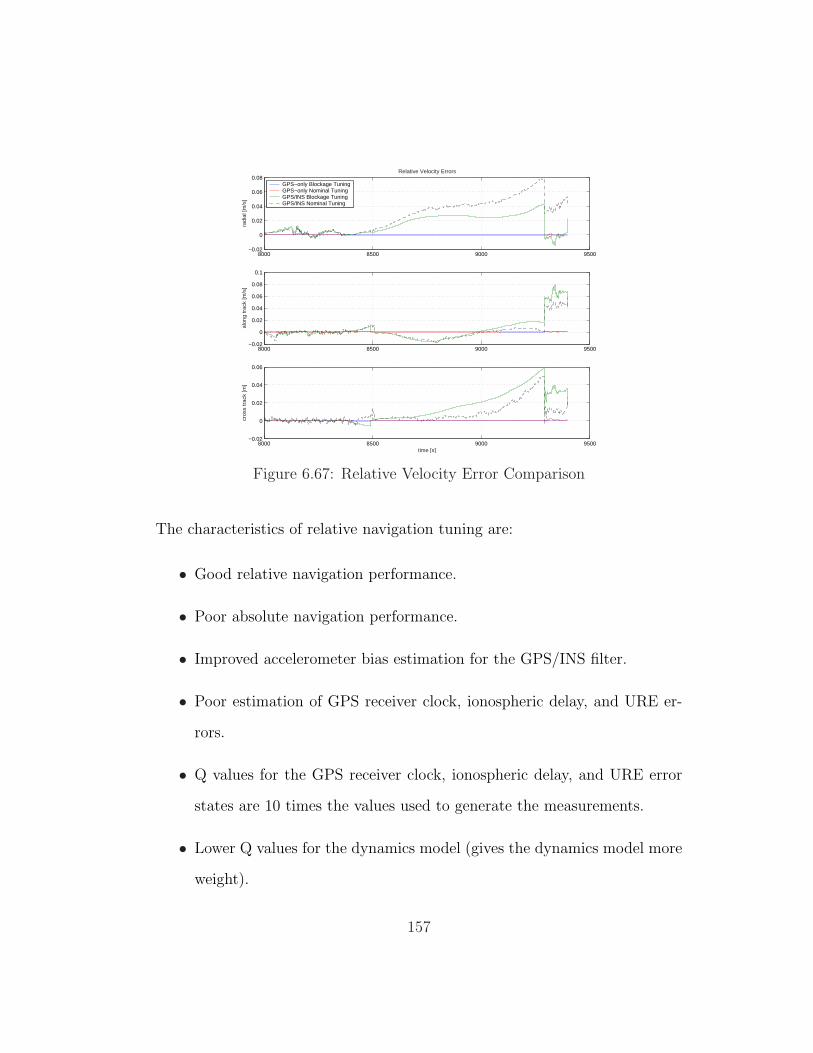
8000 8500 9000 9500−0.02

0

0.02

0.04

0.06

0.08

radi

al [m

/s]

Relative Velocity Errors

GPS−only Blockage TuningGPS−only Nominal TuningGPS/INS Blockage TuningGPS/INS Nominal Tuning

8000 8500 9000 9500−0.02

0

0.02

0.04

0.06

0.08

0.1

alon

g tr

ack

[m/s

]

8000 8500 9000 9500−0.02

0

0.02

0.04

0.06

time [s]

cros

s tr

ack

[m]

Figure 6.67: Relative Velocity Error Comparison

The characteristics of relative navigation tuning are:

• Good relative navigation performance.

• Poor absolute navigation performance.

• Improved accelerometer bias estimation for the GPS/INS filter.

• Poor estimation of GPS receiver clock, ionospheric delay, and URE er-

rors.

• Q values for the GPS receiver clock, ionospheric delay, and URE error

states are 10 times the values used to generate the measurements.

• Lower Q values for the dynamics model (gives the dynamics model more

weight).

157

The characteristics of nominal tuning are:

• Poor relative navigation performance.

• Good absolute navigation performance.

• Good estimation of GPS receiver clock, ionospheric delay, and URE er-

rors.

• Q values are set to the values used to generate the GPS measurements.

• Higher Q values for the dynamics model (gives the GPS measurements

more weight).

The navigation performance of the GPS/INS can be at least partially

explained by the filter’s ability to estimate the accelerometer biases to only

within about 1× 10−4 m/s2. If there is a constant 1× 10−4 m/s2 error in the

estimate in the accelerometer bias, it will integrate into a 50-meter position

error during a 1000-second GPS blockage. Given this analysis, the accelerom-

eter bias needs to be estimated within 2× 10−6 m/s2 per axis in order to limit

the position error to 1 meter per axis during a 1000-second GPS blockage.

Another contributing factor is the measurement of atmospheric drag

by the SIGI accelerometers. The magnitude of the specific force due to at-

mospheric drag on the chaser vehicle is approximately 1 µg. The white noise

specification of accelerometer is an indication of its sensitivity. Based on this

158

value for the SIGI accelerometer, it can be concluded that the SIGI accelerom-

eter is unable to adequately measure the effect of atmospheric drag because it

is below the SIGI accelerometer noise threshold.

The measurement of thrust by the SIGI accelerometers is also imper-

fect, even though the accelerations due to thrust are above the noise threshold.

Since the GPS-only filter was given a perfect thruster model, the GPS-only

filter is being provided better thrust information than any accelerometer could

provide. This is another contributing factor explaining the better navigation

performance of the GPS-only filter

6.2.4 Constellation Geometry and Approach Directions

The effects of GPS constellation geometry and the rendezvous approach

direction were studied. The GPS constellation was moved forward in time

to obtain four different geometrical configurations. The R-bar and V-bar

approaches were simulated with each GPS constellation configuration. The

number of visible GPS satellites at both the chaser and ISS for the eight com-

binations of constellation geometry and approach direction is shown in Figure

6.68.

159

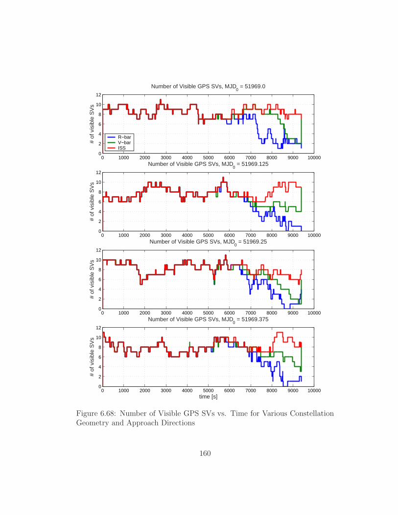
0 1000 2000 3000 4000 5000 6000 7000 8000 9000 100000

2

4

6

8

10

12#

of v

isib

le S

Vs

Number of Visible GPS SVs, MJD0 = 51969.0

R−barV−barISS

0 1000 2000 3000 4000 5000 6000 7000 8000 9000 100000

2

4

6

8

10

12

# of

vis

ible

SV

s


0 1000 2000 3000 4000 5000 6000 7000 8000 9000 100000

2

4

6

8

10

12

# of

vis

ible

SV

s


0 1000 2000 3000 4000 5000 6000 7000 8000 9000 100000

2

4

6

8

10

12

time [s]

# of

vis

ible

SV

s


Figure 6.68: Number of Visible GPS SVs vs. Time for Various ConstellationGeometry and Approach Directions

160

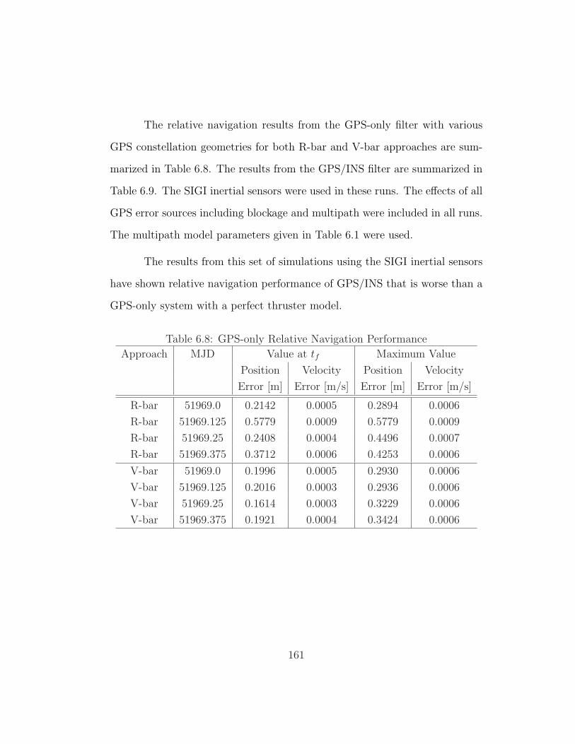
The relative navigation results from the GPS-only filter with various

GPS constellation geometries for both R-bar and V-bar approaches are sum-

marized in Table 6.8. The results from the GPS/INS filter are summarized in

Table 6.9. The SIGI inertial sensors were used in these runs. The effects of all

GPS error sources including blockage and multipath were included in all runs.

The multipath model parameters given in Table 6.1 were used.

The results from this set of simulations using the SIGI inertial sensors

have shown relative navigation performance of GPS/INS that is worse than a

GPS-only system with a perfect thruster model.

Table 6.8: GPS-only Relative Navigation Performance

Approach MJD Value at tf Maximum Value



R-bar 51969.0 0.2142 0.0005 0.2894 0.0006

R-bar 51969.125 0.5779 0.0009 0.5779 0.0009

R-bar 51969.25 0.2408 0.0004 0.4496 0.0007

R-bar 51969.375 0.3712 0.0006 0.4253 0.0006

V-bar 51969.0 0.1996 0.0005 0.2930 0.0006

V-bar 51969.125 0.2016 0.0003 0.2936 0.0006

V-bar 51969.25 0.1614 0.0003 0.3229 0.0006

V-bar 51969.375 0.1921 0.0004 0.3424 0.0006

161

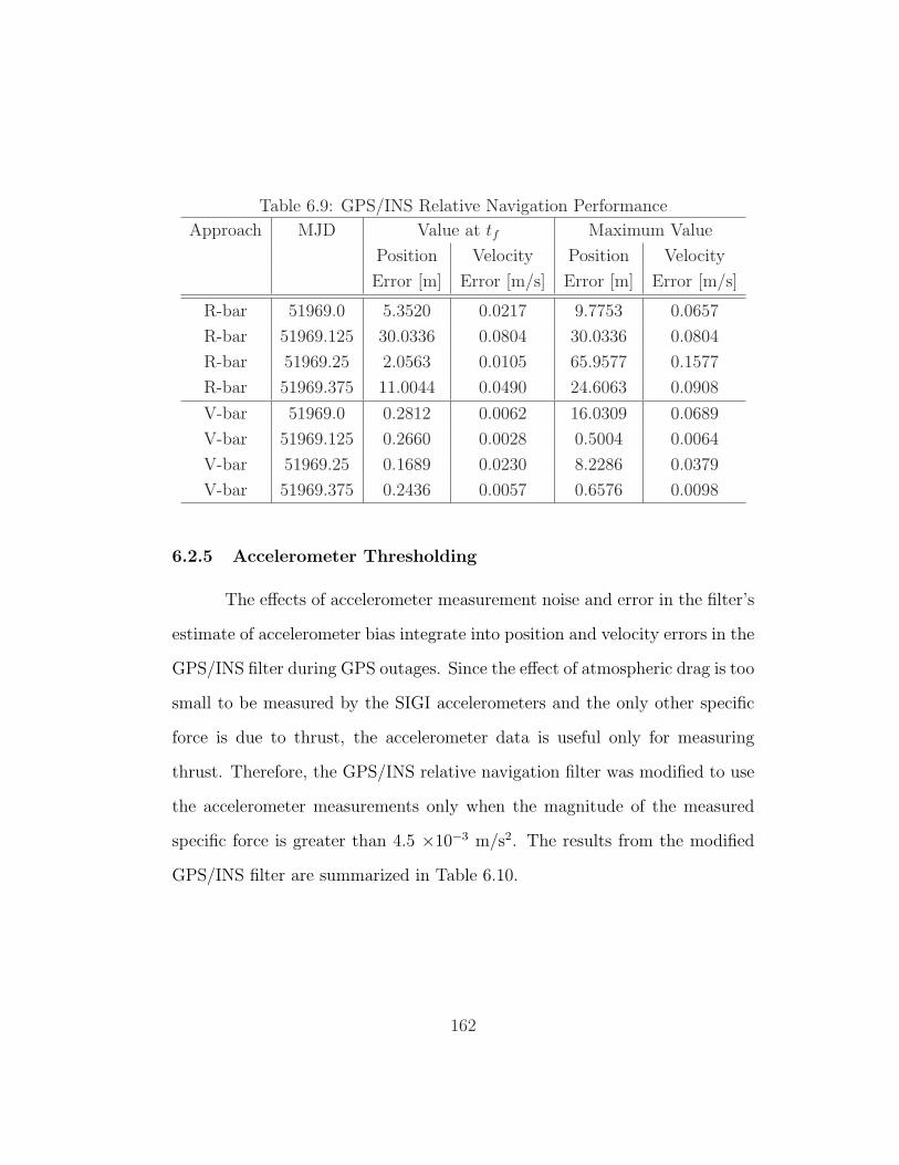
Table 6.9: GPS/INS Relative Navigation Performance




R-bar 51969.0 5.3520 0.0217 9.7753 0.0657

R-bar 51969.125 30.0336 0.0804 30.0336 0.0804

R-bar 51969.25 2.0563 0.0105 65.9577 0.1577

R-bar 51969.375 11.0044 0.0490 24.6063 0.0908

V-bar 51969.0 0.2812 0.0062 16.0309 0.0689

V-bar 51969.125 0.2660 0.0028 0.5004 0.0064

V-bar 51969.25 0.1689 0.0230 8.2286 0.0379

V-bar 51969.375 0.2436 0.0057 0.6576 0.0098

6.2.5 Accelerometer Thresholding

The effects of accelerometer measurement noise and error in the filter’s

estimate of accelerometer bias integrate into position and velocity errors in the

GPS/INS filter during GPS outages. Since the effect of atmospheric drag is too

small to be measured by the SIGI accelerometers and the only other specific

force is due to thrust, the accelerometer data is useful only for measuring

thrust. Therefore, the GPS/INS relative navigation filter was modified to use

the accelerometer measurements only when the magnitude of the measured

specific force is greater than 4.5 ×10−3 m/s2. The results from the modified

GPS/INS filter are summarized in Table 6.10.

162

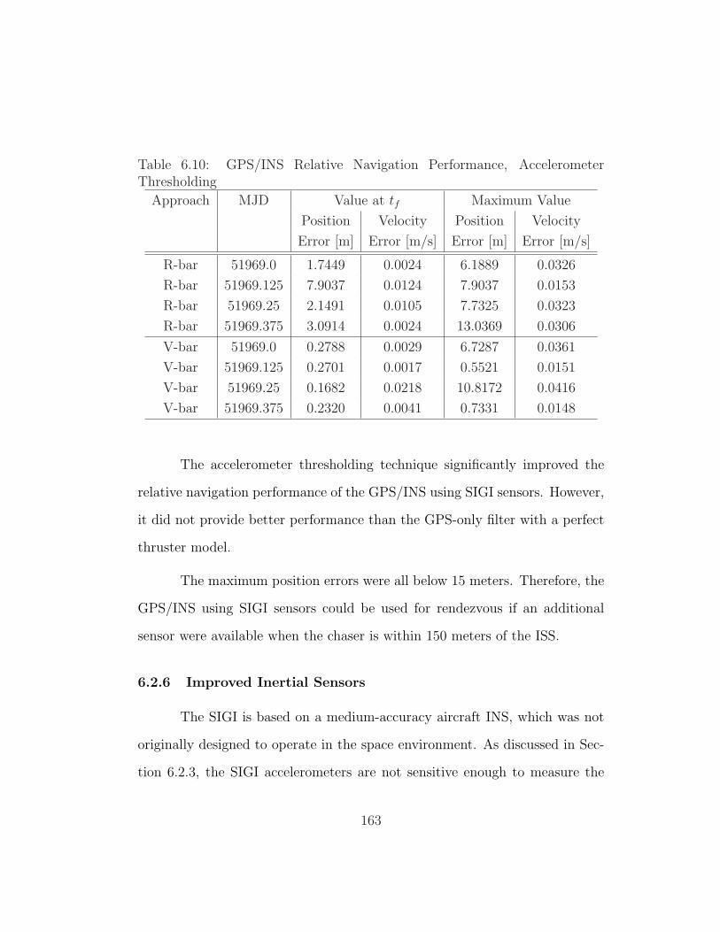
Table 6.10: GPS/INS Relative Navigation Performance, AccelerometerThresholding




R-bar 51969.0 1.7449 0.0024 6.1889 0.0326

R-bar 51969.125 7.9037 0.0124 7.9037 0.0153

R-bar 51969.25 2.1491 0.0105 7.7325 0.0323

R-bar 51969.375 3.0914 0.0024 13.0369 0.0306

V-bar 51969.0 0.2788 0.0029 6.7287 0.0361

V-bar 51969.125 0.2701 0.0017 0.5521 0.0151

V-bar 51969.25 0.1682 0.0218 10.8172 0.0416

V-bar 51969.375 0.2320 0.0041 0.7331 0.0148

The accelerometer thresholding technique significantly improved the

relative navigation performance of the GPS/INS using SIGI sensors. However,

it did not provide better performance than the GPS-only filter with a perfect

thruster model.

The maximum position errors were all below 15 meters. Therefore, the

GPS/INS using SIGI sensors could be used for rendezvous if an additional

sensor were available when the chaser is within 150 meters of the ISS.

6.2.6 Improved Inertial Sensors

The SIGI is based on a medium-accuracy aircraft INS, which was not

originally designed to operate in the space environment. As discussed in Sec-

tion 6.2.3, the SIGI accelerometers are not sensitive enough to measure the

163

effects of atmospheric drag.

The poor relative navigation performance by the GPS/INS shown in

the previous section does not mean that GPS/INS for rendezvous with the ISS

is not feasible with current technology since better gyros and accelerometers

are available. The results of simulations with these better sensors will be

supplied in this section.

A hypothetical set of inertial sensors, which will be referred to as the

Spacecraft Inertial Measurement Unit (SIMU), was modelled. The SIMU gyro

is based on the specifications of a Honeywell fiber optic gyro given in Sanders

[39]. The SIMU accelerometer is based on specifications from the accelerome-

ter used on the Gravity Recovery and Climate Experiment (GRACE) satellite.

This accelerometer has been specifically designed for measuring specific forces

in orbit and has a measurement noise specification of 1.0×10−10m/s2/rt-Hz.

Since the accelerometer bias, scale factor, and misalignment characteristics of

this accelerometer have not yet been published, the scale factor and misalign-

ment values are derived from a number of papers on MEMS micro-gravity

accelerometers, including Liu [28] and Roszhart [37]. The parameters pre-

sented in Table 6.11 were used to simulate the gyros and accelerometers of the

SIMU.

164

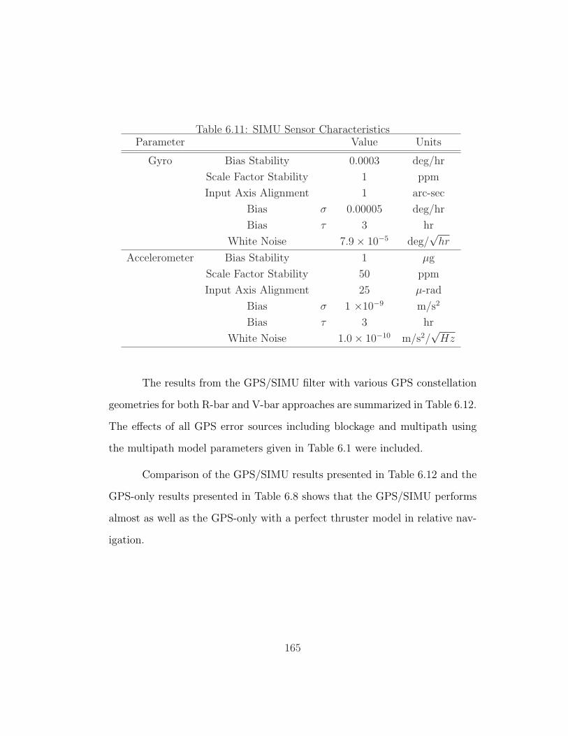
Table 6.11: SIMU Sensor CharacteristicsParameter Value Units

Gyro Bias Stability 0.0003 deg/hr


Input Axis Alignment 1 arc-sec

Bias σ 0.00005 deg/hr

Bias τ 3 hr

White Noise 7.9× 10−5 deg/√

hr

Accelerometer Bias Stability 1 µg


Input Axis Alignment 25 µ-rad

Bias σ 1 ×10−9 m/s2

Bias τ 3 hr

White Noise 1.0× 10−10 m/s2/√

Hz

The results from the GPS/SIMU filter with various GPS constellation

geometries for both R-bar and V-bar approaches are summarized in Table 6.12.

The effects of all GPS error sources including blockage and multipath using

the multipath model parameters given in Table 6.1 were included.

Comparison of the GPS/SIMU results presented in Table 6.12 and the

GPS-only results presented in Table 6.8 shows that the GPS/SIMU performs

almost as well as the GPS-only with a perfect thruster model in relative nav-

igation.

165

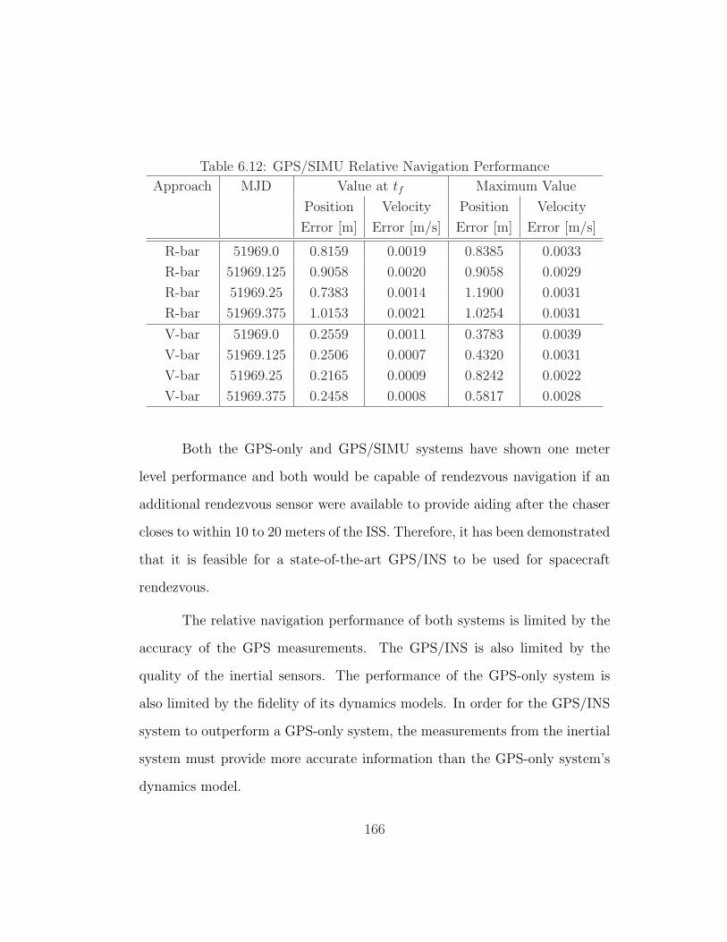
Table 6.12: GPS/SIMU Relative Navigation Performance




R-bar 51969.0 0.8159 0.0019 0.8385 0.0033

R-bar 51969.125 0.9058 0.0020 0.9058 0.0029

R-bar 51969.25 0.7383 0.0014 1.1900 0.0031

R-bar 51969.375 1.0153 0.0021 1.0254 0.0031

V-bar 51969.0 0.2559 0.0011 0.3783 0.0039

V-bar 51969.125 0.2506 0.0007 0.4320 0.0031

V-bar 51969.25 0.2165 0.0009 0.8242 0.0022

V-bar 51969.375 0.2458 0.0008 0.5817 0.0028

Both the GPS-only and GPS/SIMU systems have shown one meter

level performance and both would be capable of rendezvous navigation if an

additional rendezvous sensor were available to provide aiding after the chaser

closes to within 10 to 20 meters of the ISS. Therefore, it has been demonstrated

that it is feasible for a state-of-the-art GPS/INS to be used for spacecraft

rendezvous.

The relative navigation performance of both systems is limited by the

accuracy of the GPS measurements. The GPS/INS is also limited by the

quality of the inertial sensors. The performance of the GPS-only system is

also limited by the fidelity of its dynamics models. In order for the GPS/INS

system to outperform a GPS-only system, the measurements from the inertial

system must provide more accurate information than the GPS-only system’s

dynamics model.

166

6.2.7 Use of GPS Satellites Below the Horizon

It might be possible to improve relative navigation performance by al-

lowing the use of signals from GPS satellites below the horizon. In order

to investigate this possibility, the minimum elevation angle restriction was re-

placed with an Earth blockage cone in the blockage model. The Earth blockage

cone is defined by a sphere with a radius of 6478 km, which includes 100 km

for the atmosphere.

The blockage model for the chaser spacecraft included blockage cones

for the ISS and the Earth. The blockage model for the ISS included only an

Earth blockage cone. The results from the GPS-only filter are summarized

in Table 6.13 and the results from the GPS/INS filter using SIMU sensors

are summarized in Table 6.14. When these results are compared with those

presented in Tables 6.8 and 6.12, no consistent improvement in the relative

navigation performance is found. The additional GPS measurements did not

improve the relative navigation performance. This may be explained by the

fact that lower elevation signals are more susceptible to multipath.

167

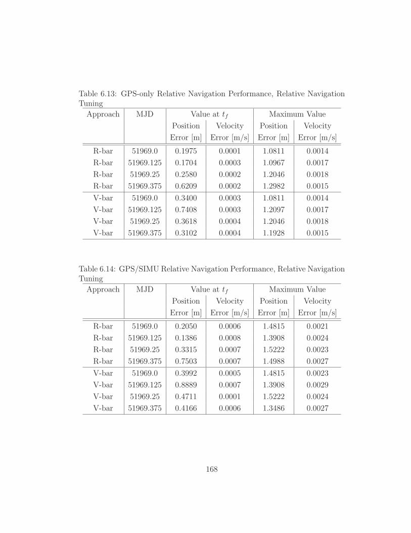
Table 6.13: GPS-only Relative Navigation Performance, Relative NavigationTuning




R-bar 51969.0 0.1975 0.0001 1.0811 0.0014

R-bar 51969.125 0.1704 0.0003 1.0967 0.0017

R-bar 51969.25 0.2580 0.0002 1.2046 0.0018

R-bar 51969.375 0.6209 0.0002 1.2982 0.0015

V-bar 51969.0 0.3400 0.0003 1.0811 0.0014

V-bar 51969.125 0.7408 0.0003 1.2097 0.0017

V-bar 51969.25 0.3618 0.0004 1.2046 0.0018

V-bar 51969.375 0.3102 0.0004 1.1928 0.0015

Table 6.14: GPS/SIMU Relative Navigation Performance, Relative NavigationTuning




R-bar 51969.0 0.2050 0.0006 1.4815 0.0021

R-bar 51969.125 0.1386 0.0008 1.3908 0.0024

R-bar 51969.25 0.3315 0.0007 1.5222 0.0023

R-bar 51969.375 0.7503 0.0007 1.4988 0.0027

V-bar 51969.0 0.3992 0.0005 1.4815 0.0023

V-bar 51969.125 0.8889 0.0007 1.3908 0.0029

V-bar 51969.25 0.4711 0.0001 1.5222 0.0024

V-bar 51969.375 0.4166 0.0006 1.3486 0.0027

168

6.2.8 Gain Scheduling

The results presented in Section 6.2.3 showed that relative navigation

performance during a rendezvous with the ISS can be improved by properly

tuning the dynamics noise. However, this improvement comes at the expense

of absolute navigation performance. It may be possible to minimize the loss

of absolute navigation performance while maintaining good relative naviga-

tion performance by changing the tuning parameters from nominal tuning to

relative navigation tuning at some point as the chaser approaches the ISS.

The GPS-only and GPS/INS filters were modified to switch from nomi-

nal tuning to relative navigation tuning two minutes before less than four GPS

SVs were visible at the chaser. The GPS-only filter used a perfect thruster

model and the GPS/INS filter used the SIMU sensors and all GPS and INS er-

ror sources were simulated for an R-bar approach. The results are summarized

in Table 6.15.

The results show improved relative navigation performance when using

gain scheduling instead of the relative navigation tuning. This suggests that

gain scheduling should be investigated further for this application.

169

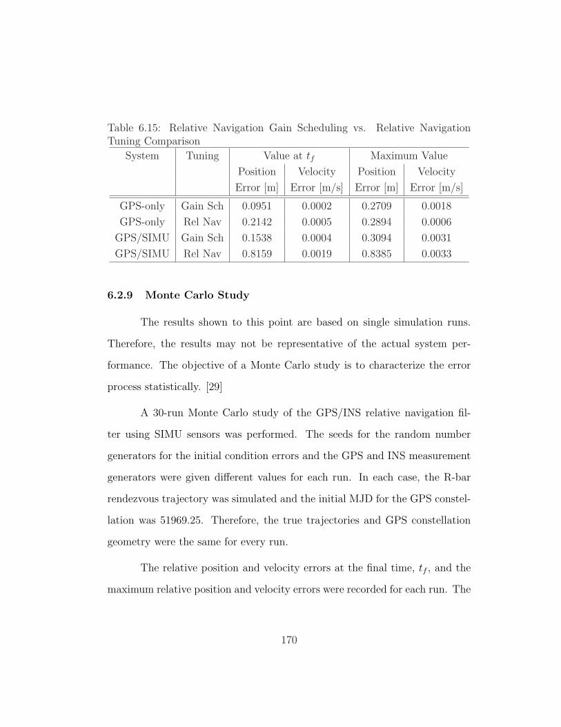
Table 6.15: Relative Navigation Gain Scheduling vs. Relative NavigationTuning Comparison

System Tuning Value at tf Maximum Value



GPS-only Gain Sch 0.0951 0.0002 0.2709 0.0018

GPS-only Rel Nav 0.2142 0.0005 0.2894 0.0006

GPS/SIMU Gain Sch 0.1538 0.0004 0.3094 0.0031

GPS/SIMU Rel Nav 0.8159 0.0019 0.8385 0.0033

6.2.9 Monte Carlo Study

The results shown to this point are based on single simulation runs.

Therefore, the results may not be representative of the actual system per-

formance. The objective of a Monte Carlo study is to characterize the error

process statistically. [29]

A 30-run Monte Carlo study of the GPS/INS relative navigation fil-

ter using SIMU sensors was performed. The seeds for the random number

generators for the initial condition errors and the GPS and INS measurement

generators were given different values for each run. In each case, the R-bar

rendezvous trajectory was simulated and the initial MJD for the GPS constel-

lation was 51969.25. Therefore, the true trajectories and GPS constellation

geometry were the same for every run.

The relative position and velocity errors at the final time, tf , and the

maximum relative position and velocity errors were recorded for each run. The

170

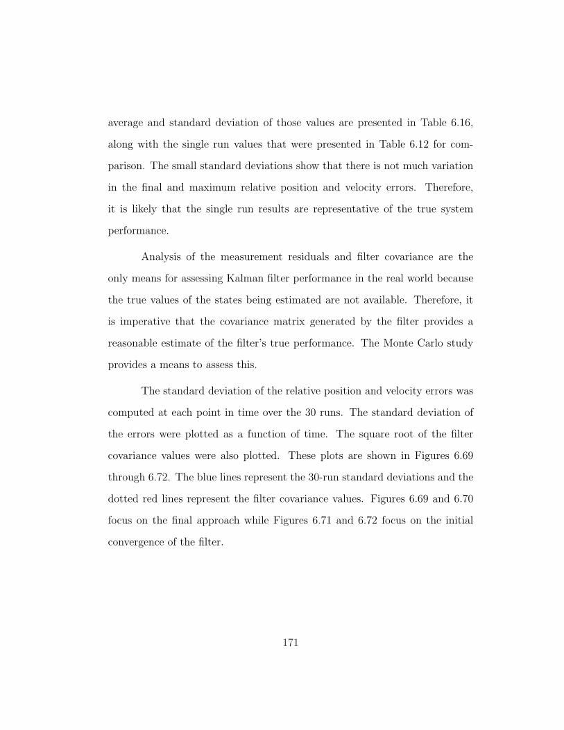
average and standard deviation of those values are presented in Table 6.16,

along with the single run values that were presented in Table 6.12 for com-

parison. The small standard deviations show that there is not much variation

in the final and maximum relative position and velocity errors. Therefore,

it is likely that the single run results are representative of the true system

performance.

Analysis of the measurement residuals and filter covariance are the

only means for assessing Kalman filter performance in the real world because

the true values of the states being estimated are not available. Therefore, it

is imperative that the covariance matrix generated by the filter provides a

reasonable estimate of the filter’s true performance. The Monte Carlo study

provides a means to assess this.

The standard deviation of the relative position and velocity errors was

computed at each point in time over the 30 runs. The standard deviation of

the errors were plotted as a function of time. The square root of the filter

covariance values were also plotted. These plots are shown in Figures 6.69

through 6.72. The blue lines represent the 30-run standard deviations and the

dotted red lines represent the filter covariance values. Figures 6.69 and 6.70

focus on the final approach while Figures 6.71 and 6.72 focus on the initial

convergence of the filter.

171

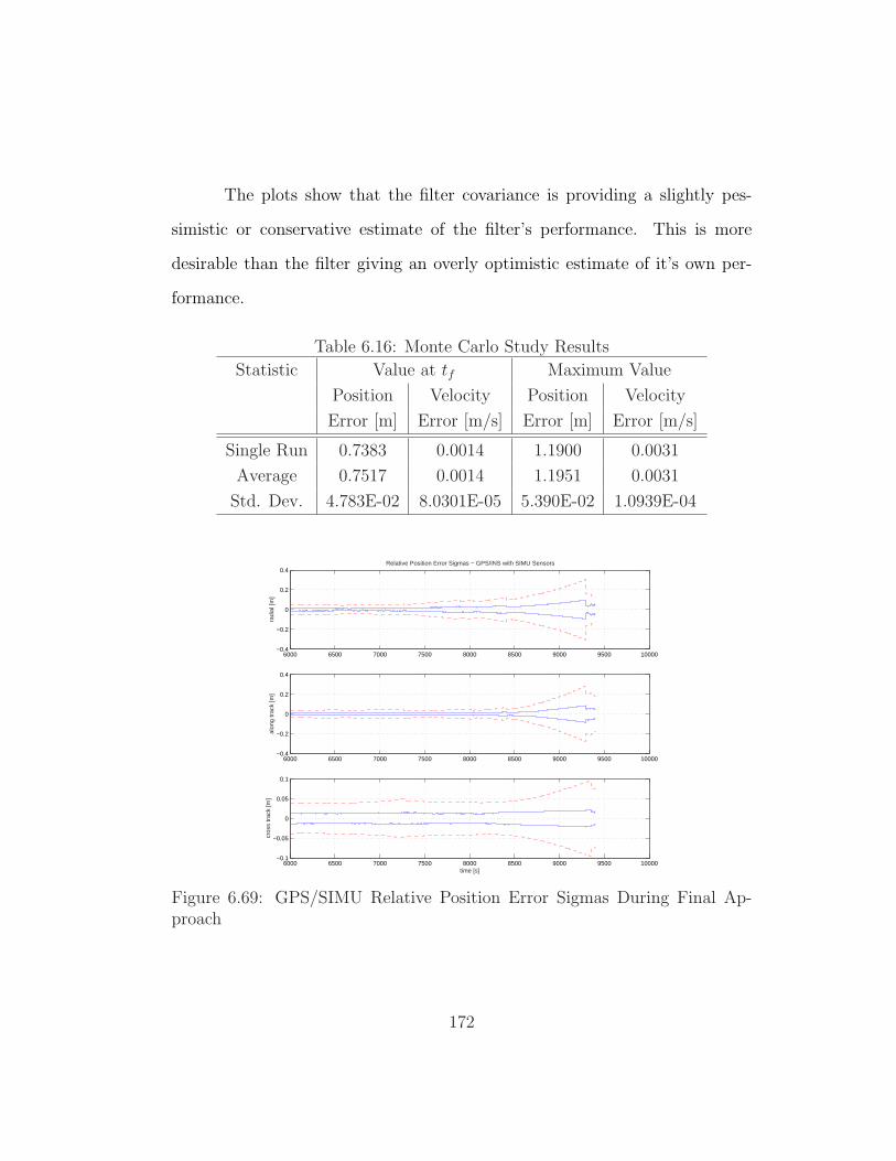
The plots show that the filter covariance is providing a slightly pes-

simistic or conservative estimate of the filter’s performance. This is more

desirable than the filter giving an overly optimistic estimate of it’s own per-

formance.

Table 6.16: Monte Carlo Study Results

Statistic Value at tf Maximum Value



Single Run 0.7383 0.0014 1.1900 0.0031

Average 0.7517 0.0014 1.1951 0.0031

Std. Dev. 4.783E-02 8.0301E-05 5.390E-02 1.0939E-04

6000 6500 7000 7500 8000 8500 9000 9500 10000−0.4

−0.2

0

0.2

0.4

radi

al [m

]

Relative Position Error Sigmas − GPS/INS with SIMU Sensors

6000 6500 7000 7500 8000 8500 9000 9500 10000−0.4

−0.2

0

0.2

0.4

alon

g tr

ack

[m]

6000 6500 7000 7500 8000 8500 9000 9500 10000−0.1

−0.05

0

0.05

0.1

time [s]

cros

s tr

ack

[m]

Figure 6.69: GPS/SIMU Relative Position Error Sigmas During Final Ap-proach

172

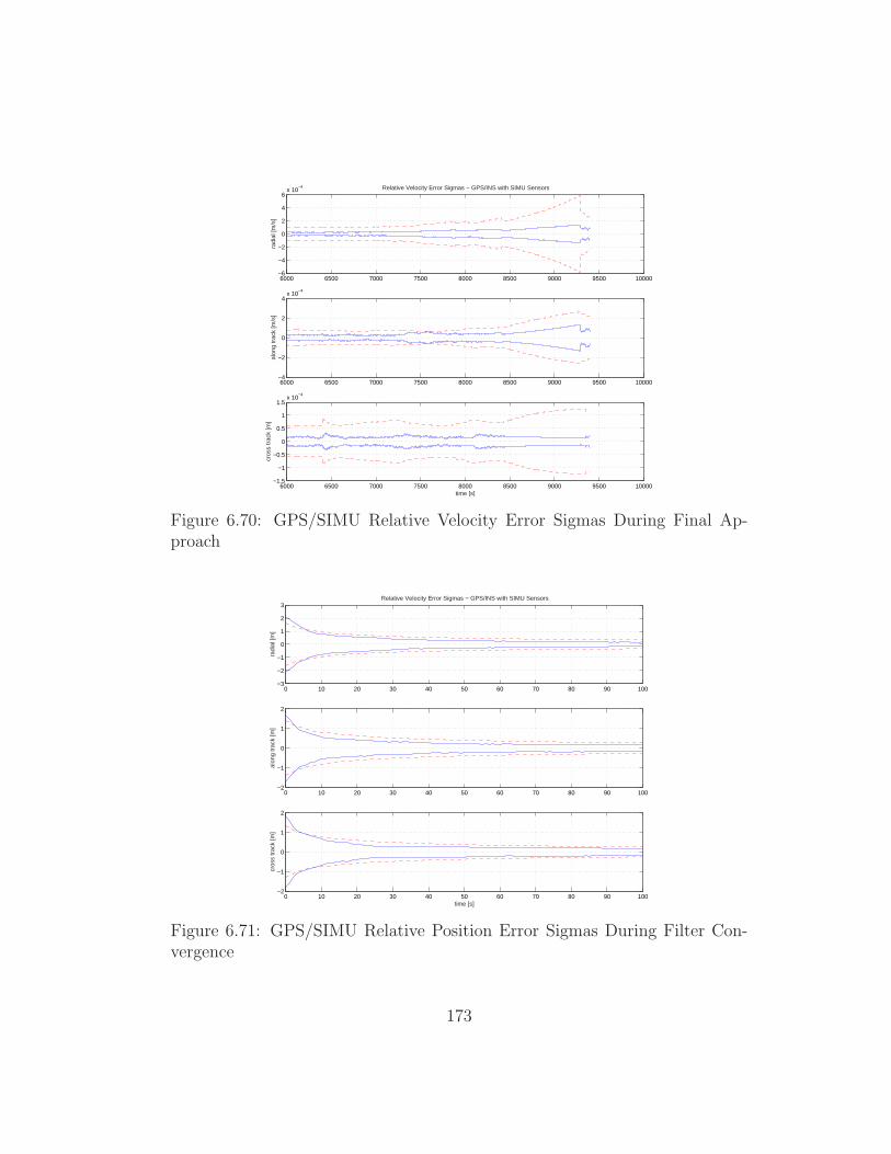
6000 6500 7000 7500 8000 8500 9000 9500 10000−6

−4

−2

0

2

4

6x 10

−4

radi

al [m

/s]

Relative Velocity Error Sigmas − GPS/INS with SIMU Sensors

6000 6500 7000 7500 8000 8500 9000 9500 10000−4

−2

0

2

4x 10

−4

alon

g tr

ack

[m/s

]

6000 6500 7000 7500 8000 8500 9000 9500 10000−1.5

−1

−0.5

0

0.5

1

1.5x 10

−4

time [s]

cros

s tr

ack

[m]

Figure 6.70: GPS/SIMU Relative Velocity Error Sigmas During Final Ap-proach

0 10 20 30 40 50 60 70 80 90 100−3

−2

−1

0

1

2

3

radi

al [m

]


0 10 20 30 40 50 60 70 80 90 100−2

−1

0

1

2

alon

g tr

ack

[m]

0 10 20 30 40 50 60 70 80 90 100−2

−1

0

1

2

time [s]

cros

s tr

ack

[m]

Figure 6.71: GPS/SIMU Relative Position Error Sigmas During Filter Con-vergence

173

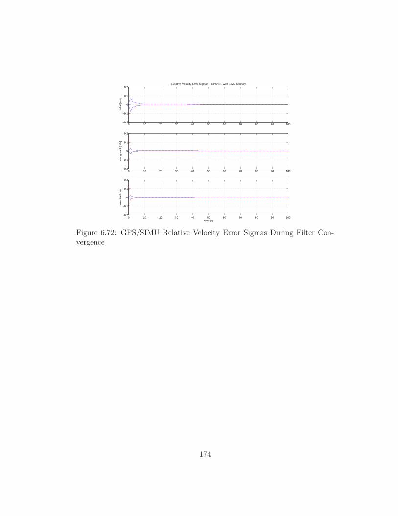
0 10 20 30 40 50 60 70 80 90 100−0.2

−0.1

0

0.1

0.2

radi

al [m

/s]


0 10 20 30 40 50 60 70 80 90 100−0.2

−0.1

0

0.1

0.2

alon

g tr

ack

[m/s

]

0 10 20 30 40 50 60 70 80 90 100−0.2

−0.1

0

0.1

0.2

time [s]

cros

s tr

ack

[m]

Figure 6.72: GPS/SIMU Relative Velocity Error Sigmas During Filter Con-vergence

174

Chapter 7

Conclusions

The objective of this research is to determine if GPS/INS navigation

during a rendezvous with the ISS is feasible with existing inertial sensor tech-

nology and if not, determine the requirements for future GPS and inertial

sensor technology to make it feasible. This chapter provides a summary of the

results and suggests topics for future research.

7.1 Summary of Results

The results of the relative navigation simulations demonstrate that both

the GPS-only and GPS/INS systems can achieve one meter level relative nav-

igation accuracy during rendezvous with the ISS. Therefore, it is feasible to

use GPS/INS for rendezvous with ISS if state-of-the-art inertial sensors are

used and if an additional rendezvous sensor were available to provide aiding

after the chaser closes to within 10 to 20 meters of the ISS. These simulations

included all significant GPS and INS error sources as well as a high-fidelity

representation of realistic ISS rendezvous trajectories. They also included re-

alistic models of GPS signal blockage and multipath near the ISS.

In order to obtain these results, an error model for an INS operating

175

in orbit has been developed. This model has been used to characterize the

behavior on an INS in orbit. This characterization can be used to understand

how accelerometer and gyro errors affect inertial navigation performance in

space.

A simple model of the blockage of GPS signals by the ISS has been

developed and the effect on GPS navigation near the ISS has been studied. The

blockage simulation showed that aiding of GPS is needed when the spacecraft

approaches within 60 meters the ISS. The multipath simulation results show

the expected trends in the range errors as a function of the GPS satellite

elevation angle, distance from the ISS, the number of multipath rays modelled,

and the radar cross-sectional area of the ISS. Both effects may significantly

degrade GPS navigation near the ISS. These models can be used to predict the

performance obtained by combining various sensors with GPS for navigation

or attitude determination for spacecraft operating near the ISS or other large

reflecting body.

A new statistical multipath model for spacecraft operating near the ISS

has been developed based on terrestrial urban and indoor multipath models.

The model characterizes the multipath environment in terms of the amplitudes,

time delays and phases of the multipath signals, which are used by the C/A

code and carrier phase measurement error models to determine the error in

GPS range measurements.

A complementary extended Kalman filter (EKF) for combining GPS

and INS measurements has been developed. The INS measurements provide

176

the reference trajectory for the EKF, which computes corrections to the ref-

erence trajectory. The reference trajectory is updated with these corrections

each filter cycle. Both absolute and relative navigation filters have been de-

veloped.

During the development of the absolute navigation filter, the navigation

results of GPS C/A code measurements were compared to those resulting

from the use of GPS carrier phase measurements. For absolute navigation,

it was determined that while GPS carrier phase measurements were more

precise than C/A code measurements, the navigation accuracy was actually

better using C/A code measurements. The reason for this is that in the case

of absolute navigation, the filter was not able to adequately allocate errors

between ionospheric delay, GPS SV clock and ephemeris errors, and the integer

ambiguity.

One of the decisions to be made in the development of a GPS relative

navigation system is whether to exchange measurement data or processed state

data. The simulation showed that processing measurements from both chaser

and target vehicles provides an order of magnitude improvement in relative

navigation accuracy over the the use of state vector differencing.

The inertial sensors come into play mostly during the final phase of

rendezvous, where GPS signals are blocked and are subject to multipath and

many small delta-v and attitude maneuvers that disturb the GPS tracking

loops. To demonstrate the value of the INS during this time, a realistic ren-

dezvous simulation was developed which includes the effects of gravity and

177

atmospheric drag perturbations as well as delta-v maneuvers planned to cre-

ate a decelerating glideslope trajectory. The results of a GPS-only relative

navigation filter, the GPS/INS relative navigation filter with the SIGI gyros

and accelerometers, and the GPS/INS relative navigation filter with improved

gyros and accelerometers were analyzed and compared.

The effects of filter tuning on the performance of the relative navigation

filters were studied. The results show that filter tuning has a large effect on

the relative navigation accuracy of both the GPS-only and GPS/INS filters.

The effects of GPS constellation geometry and the rendezvous approach

direction were studied. The GPS constellation was moved forward in time to

obtain four different geometrical configurations. The R-bar and V-bar ap-

proach were simulated with each GPS constellation configuration. The results

of this analysis showed that the relative navigation performance is highly de-

pendent on GPS constellation geometry and approach direction.

The results from the simulations using the SIGI sensors have shown that

relative navigation performance of the GPS/INS is not adequate for rendezvous

and is actually worse than a GPS-only system with a perfect thruster model.

The relative navigation performance of the GPS/INS filter during GPS

blockage is limited by the filter’s ability to estimate accelerometer bias. In

order to limit the position error to 1 meter per axis during a 1000-second GPS

blockage, the accelerometer bias needs to be estimated within 2× 10−6 m/s2.

The use of accelerometer thresholding was shown to significantly im-

178

prove the performance of the GPS/INS relative navigation filter using SIGI

sensors. In this case, the maximum relative position error was below 15 me-

ters. Therefore, it would be feasible to use the GPS/INS with SIGI sensors

if an additional rendezvous sensor were available to provide aiding after the

chaser closes to within 150 meters of the ISS.

Comparison of a GPS/INS using state-of-the-art inertial sensors with

a GPS-only filter with a perfect thruster model shows that the improved

GPS/INS performs almost as well as the GPS-only system in relative navi-

gation. Research on micromechanical accelerometers and fiber optic gyros is

likely to yield even better inertial sensors. With these sensors, a GPS/INS will

be able to outperform a GPS-only system in the future.

The accelerometer used on-orbit probably could not be used during the

other flight phases because highly sensitive accelerometers would not become

saturated at high levels of specific force. However, the mass penalty of carrying

two sets of accelerometers would be small if micromechanical accelerometers

are used.

The relative navigation performance of both GPS/INS and GPS-only

navigation systems is limited by the accuracy of the GPS measurements. The

GPS/INS is also limited by the accuracy of the inertial sensors. The perfor-

mance of the GPS-only system is also limited by the fidelity of its dynamics

models. In order for the GPS/INS system to outperform a GPS-only sys-

tem, the measurements from the inertial system must provide more accurate

information than the GPS-only system’s dynamics model.

179

The GPS-only system’s dynamics model for a spacecraft in orbit can be

very accurate if there are no unexpected forces acting on the spacecraft, such

as an unbalanced force due to attitude control thrusters. One of the benefits

of having inertial sensors onboard is that they would be able to sense the un-

expected forces and maintain accurate navigation. This makes the GPS/INS a

more robust solution than the GPS-only, which is needed for manned missions.

Two possible improvements to the relative navigation filters were also

investigated. The use of GPS satellites below the horizon was found not to pro-

vide any improvement to relative navigation performance during a rendezvous

with the ISS.

The other improvement was the use of gain scheduling, where the pro-

cess noise is switched during the flight. This was found to provide some im-

provement in relative navigation performance. Therefore, it is recommended

that gain scheduling be investigated in the future.

The effects of GPS signal blockage and multipath near the ISS on GPS

and GPS/INS navigation are the main focus of this research. However, many

of the results and lessons learned can be applied to other two spacecraft ren-

dezvous problems. For example, during a Hubble telescope servicing mission,

multipath signals reflected off of the telescope could be modelled using the ISS

multipath model.

180

7.2 Future Work

The results of the relative navigation filter simulations suggest that a

different filter formulation may potentially produce better relative navigation

results in periods of GPS blockage. The current filter formulation estimates

the absolute position and velocity of the chaser and target, however, a special

rendezvous filter that estimates the relative position and relative velocity may

be more ideally suited to this problem. But an absolute navigation filter would

still be required for some on-orbit operations.

Another possible approach would be to use a filter that varies the mea-

surement or process noise according to the number of GPS satellites in view.

When there are four or more GPS satellites in view, the filter solution would

put more weight on the measurements, when fewer than four GPS satellites

are in view, the filter would rely more on the dynamics model. Various switch-

ing criteria, such as number of visible GPS satellites and distance from ISS,

should be studied to determine the optimal switching criteria.

Standard avionics-grade accelerometers and gyros are not designed for

space applications, where specific forces are very small and attitude rates are

low. In order to increase the effectiveness of GPS/INS in space, accelerometers

and gyros need to be more sensitive (lower measurement noise) and have well

known and predictable run-to-run and in-run bias behavior. The unique sensor

requirements for accelerometers and gyros operating in space should be studied

and documented. The new sensor requirements will likely require new test

methods and equipment in order to verify on-orbit sensor performance. These

181

new test methods and equipment requirements may also necessitate further

research and development.

Another possible configuration that should be examined is a gyro-free

GPS/INS, where the GPS would be aided by accelerometers with attitude

provided by GPS or some other attitude sensor. This could potentially improve

performance or reduce cost, weight, and power requirements as well as increase

reliability.

In this dissertation, it was assumed that both the chaser and target

vehicle were each equipped with a single, zenith-pointed antenna and that the

spacecraft always maintained the zenith-pointed attitude. In a rendezvous

scenario, the attitude of the spacecraft is just as important as its position

and velocity. Therefore, the addition of spacecraft attitude modelling would

greatly enhance the value of the GPS/INS rendezvous simulation. Further-

more, the ability to study multiple GPS antennas and various GPS antenna

locations could potentially allow designers to minimize the effects of blockage

and multipath.

The GPS/INS simulation assumed that the GPS receiver is immediately

able to resume tracking satellites after an outage due to blockage, which is not

realistic. In a tightly integrated GPS/INS, the GPS receiver tracking loops

are aided by the INS so that it can recover faster. Therefore, a tracking loop

simulation capability should be added.

182

The incorporation of better models for the GPS SV clock and ephemeris

errors, ionospheric delays and the addition of cycle slips would improve the

fidelity of the simulation.

The blockage and multipath models presented in this dissertation are

theoretical and have not been validated with flight data. After numerous dis-

cussion with engineers at the NASA Johnson Space Center, it was determined

that the data needed to validate these models currently does not exist. With-

out this data, engineers are designing autonomous rendezvous systems “in the

blind.” Therefore, it is recommended that a flight experiment specifically de-

signed to collect GPS multipath and blockage information in the vicinity of

the ISS be performed as soon as possible.

Researchers have developed many ways to minimize the effects of mul-

tipath on GPS navigation. Some of these methods include special antennas,

correlators and processing software. For example, the filter could be modified

to increase the measurement noise as the chaser approaches the ISS. The ef-

fectiveness of these techniques in the rendezvous scenario could be evaluated

using this simulation.

The effects of signal blockage near the ISS could possibly be reduced by

the addition of measurements from GLONASS or Galileo in the future. The

GPS/INS simulation could also be used to study the addition of rendezvous

sensors such as pseudolites or optical sensors to mitigate the effects of blockage

and multipath.

183

Another possible way to improve the navigation performance near the

ISS might be to allow the use of GPS signals within the ISS blockage cone

since the ISS is not a solid spherical shape. One way to simulate this would be

to randomly allow a certain percentage of the signals within the ISS blockage

cone to be used.

Finally, this simulation could be used to study the emergency egress

from ISS scenario. In this case, the GPS/INS would be required to initialize

and align itself in flight. The GPS signal blockage due to the ISS could have a

significant impact on the time required to lock on to four GPS satellites. This

may impact the ability to perform the de-orbit maneuver in an accurate and

timely manner.

184

Appendices

185

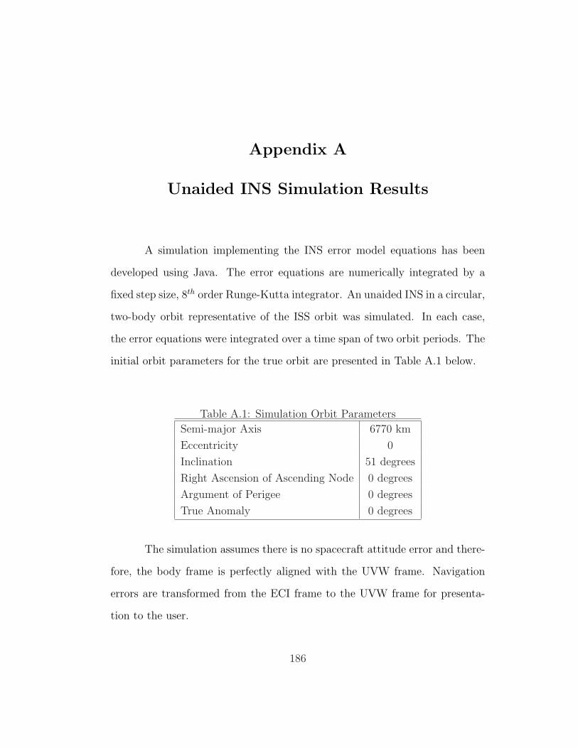
Appendix A

Unaided INS Simulation Results

A simulation implementing the INS error model equations has been

developed using Java. The error equations are numerically integrated by a

fixed step size, 8th order Runge-Kutta integrator. An unaided INS in a circular,

two-body orbit representative of the ISS orbit was simulated. In each case,

the error equations were integrated over a time span of two orbit periods. The

initial orbit parameters for the true orbit are presented in Table A.1 below.

Table A.1: Simulation Orbit Parameters

Semi-major Axis 6770 km

Eccentricity 0

Inclination 51 degrees

Right Ascension of Ascending Node 0 degrees

Argument of Perigee 0 degrees

True Anomaly 0 degrees

The simulation assumes there is no spacecraft attitude error and there-

fore, the body frame is perfectly aligned with the UVW frame. Navigation

errors are transformed from the ECI frame to the UVW frame for presenta-

tion to the user.

186

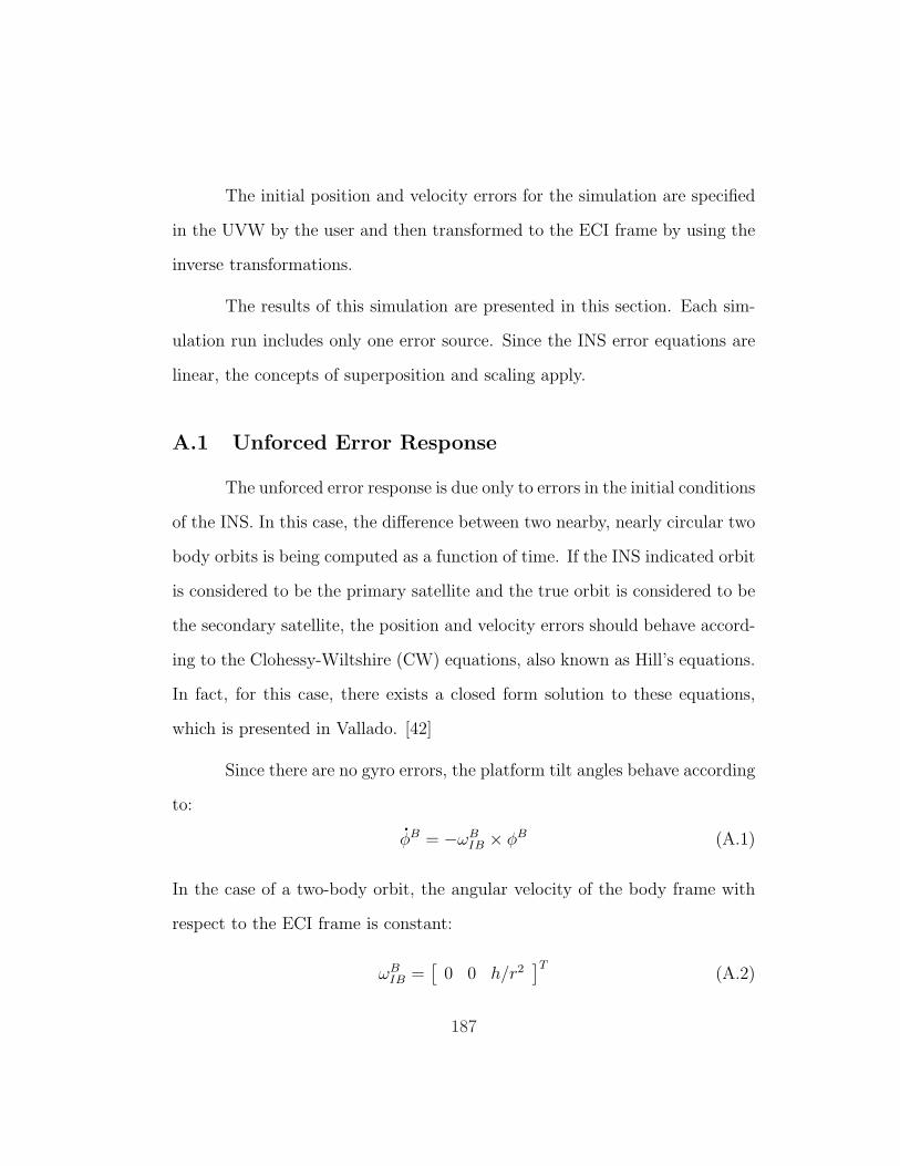
The initial position and velocity errors for the simulation are specified

in the UVW by the user and then transformed to the ECI frame by using the

inverse transformations.

The results of this simulation are presented in this section. Each sim-

ulation run includes only one error source. Since the INS error equations are

linear, the concepts of superposition and scaling apply.

A.1 Unforced Error Response

The unforced error response is due only to errors in the initial conditions

of the INS. In this case, the difference between two nearby, nearly circular two

body orbits is being computed as a function of time. If the INS indicated orbit

is considered to be the primary satellite and the true orbit is considered to be

the secondary satellite, the position and velocity errors should behave accord-

ing to the Clohessy-Wiltshire (CW) equations, also known as Hill’s equations.

In fact, for this case, there exists a closed form solution to these equations,

which is presented in Vallado. [42]

Since there are no gyro errors, the platform tilt angles behave according

to:

φB = −ωBIB × φB (A.1)

In the case of a two-body orbit, the angular velocity of the body frame with

respect to the ECI frame is constant:

ωBIB =

[0 0 h/r2

]T(A.2)

187

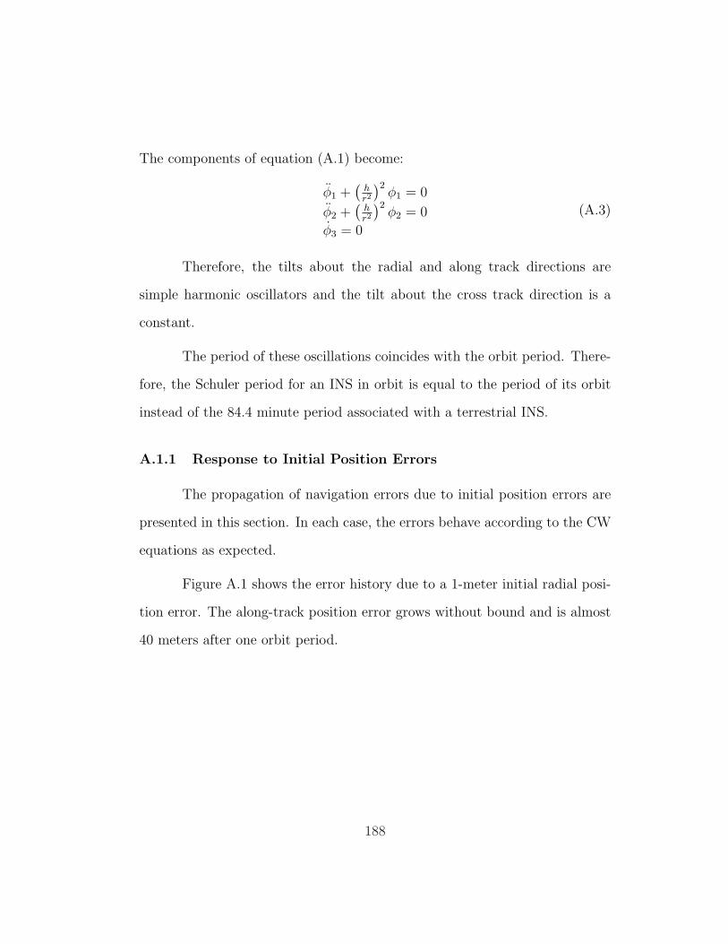
The components of equation (A.1) become:

φ1 +(

hr2

)2φ1 = 0

φ2 +(

hr2

)2φ2 = 0

φ3 = 0

(A.3)

Therefore, the tilts about the radial and along track directions are

simple harmonic oscillators and the tilt about the cross track direction is a

constant.

The period of these oscillations coincides with the orbit period. There-

fore, the Schuler period for an INS in orbit is equal to the period of its orbit

instead of the 84.4 minute period associated with a terrestrial INS.

A.1.1 Response to Initial Position Errors

The propagation of navigation errors due to initial position errors are

presented in this section. In each case, the errors behave according to the CW

equations as expected.

Figure A.1 shows the error history due to a 1-meter initial radial posi-

tion error. The along-track position error grows without bound and is almost

40 meters after one orbit period.

188

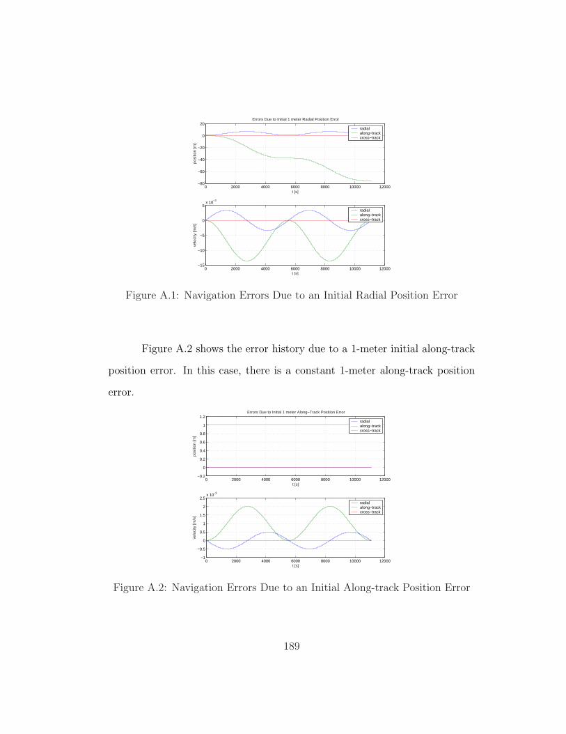
0 2000 4000 6000 8000 10000 12000−80

−60

−40

−20

0

20

t [s]po

sitio

n [m

]

Errors Due to Initial 1 meter Radial Position Error


0 2000 4000 6000 8000 10000 12000−15

−10

−5

0

5x 10

−3

t [s]

velo

city

[m/s

]


Figure A.1: Navigation Errors Due to an Initial Radial Position Error

Figure A.2 shows the error history due to a 1-meter initial along-track

position error. In this case, there is a constant 1-meter along-track position

error.

0 2000 4000 6000 8000 10000 12000−0.2

0

0.2

0.4

0.6

0.8

1

1.2

t [s]

posi

tion

[m]

Errors Due to Initial 1 meter Along−Track Position Error


0 2000 4000 6000 8000 10000 12000−1

−0.5

0

0.5

1

1.5

2

2.5x 10

−9

t [s]

velo

city

[m/s

]


Figure A.2: Navigation Errors Due to an Initial Along-track Position Error

189

Figure A.3 shows the error history due to a 1-meter initial cross-track

position error. In this case, the cross-track position error oscillates between

+1 and -1 meters with a period coincident with the orbit period. No radial or

along-track errors are induced because the cross-track direction is not coupled

with the other directions.

0 2000 4000 6000 8000 10000 12000−1

−0.5

0

0.5

1

t [s]

posi

tion

[m]

Errors Due to Initial 1 meter Cross−Track Position Error


0 2000 4000 6000 8000 10000 12000−1.5

−1

−0.5

0

0.5

1

1.5x 10

−3

t [s]

velo

city

[m/s

]


Figure A.3: Navigation Errors Due to an Initial Cross-track Position Error

A.1.2 Response to Initial Velocity Errors

The propagation of navigation errors due to initial velocity errors are

presented in this section. In each case, the errors behave according to the CW

equations as expected.

Figure A.4 shows the error history due to a 0.1-m/s initial radial ve-

locity error. In this case, large but stable position errors are observed. The

radial position error oscillates between +100 and -100 meters and the along-

190

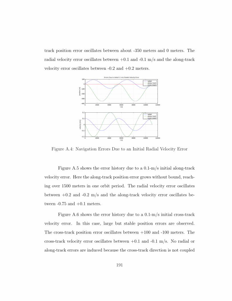
track position error oscillates between about -350 meters and 0 meters. The

radial velocity error oscillates between +0.1 and -0.1 m/s and the along-track

velocity error oscillates between -0.2 and +0.2 meters.

0 2000 4000 6000 8000 10000 12000−400

−300

−200

−100

0

100

t [s]

posi

tion

[m]

Errors Due to Initial 0.1 m/s Radial Velocity Error


0 2000 4000 6000 8000 10000 12000−0.2

−0.1

0

0.1

0.2

t [s]

velo

city

[m/s

]


Figure A.4: Navigation Errors Due to an Initial Radial Velocity Error

Figure A.5 shows the error history due to a 0.1-m/s initial along-track

velocity error. Here the along-track position error grows without bound, reach-

ing over 1500 meters in one orbit period. The radial velocity error oscillates

between +0.2 and -0.2 m/s and the along-track velocity error oscillates be-

tween -0.75 and +0.1 meters.

Figure A.6 shows the error history due to a 0.1-m/s initial cross-track

velocity error. In this case, large but stable position errors are observed.

The cross-track position error oscillates between +100 and -100 meters. The

cross-track velocity error oscillates between +0.1 and -0.1 m/s. No radial or

along-track errors are induced because the cross-track direction is not coupled

191

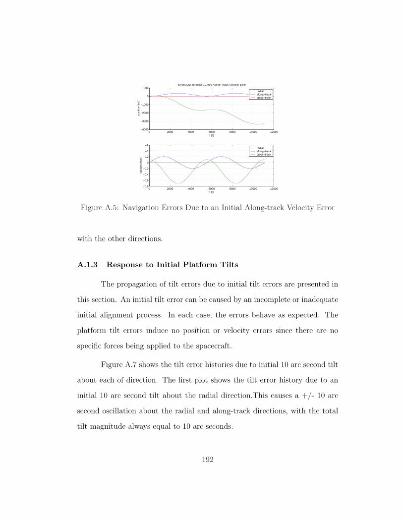
0 2000 4000 6000 8000 10000 12000−4000

−3000

−2000

−1000

0

1000

t [s]po

sitio

n [m

]

Errors Due to Initial 0.1 m/s Along−Track Velocity Error


0 2000 4000 6000 8000 10000 12000−0.8

−0.6

−0.4

−0.2

0

0.2

0.4

0.6

t [s]

velo

city

[m/s

]


Figure A.5: Navigation Errors Due to an Initial Along-track Velocity Error

with the other directions.

A.1.3 Response to Initial Platform Tilts

The propagation of tilt errors due to initial tilt errors are presented in

this section. An initial tilt error can be caused by an incomplete or inadequate

initial alignment process. In each case, the errors behave as expected. The

platform tilt errors induce no position or velocity errors since there are no

specific forces being applied to the spacecraft.

Figure A.7 shows the tilt error histories due to initial 10 arc second tilt

about each of direction. The first plot shows the tilt error history due to an

initial 10 arc second tilt about the radial direction.This causes a +/- 10 arc

second oscillation about the radial and along-track directions, with the total

tilt magnitude always equal to 10 arc seconds.

192

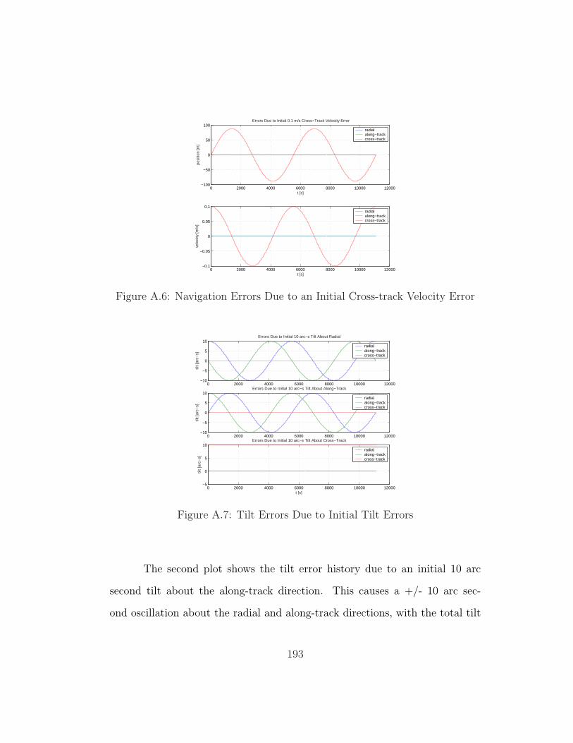
0 2000 4000 6000 8000 10000 12000−100

−50

0

50

100

t [s]po

sitio

n [m

]

Errors Due to Initial 0.1 m/s Cross−Track Velocity Error


0 2000 4000 6000 8000 10000 12000−0.1

−0.05

0

0.05

0.1

t [s]

velo

city

[m/s

]


Figure A.6: Navigation Errors Due to an Initial Cross-track Velocity Error

0 2000 4000 6000 8000 10000 12000−10

−5

0

5

10

tilt [

arc−

s]

Errors Due to Initial 10 arc−s Tilt About Radial


0 2000 4000 6000 8000 10000 12000−10

−5

0

5

10

tilt [

arc−

s]

Errors Due to Initial 10 arc−s Tilt About Along−Track


0 2000 4000 6000 8000 10000 12000−5

0

5

10

t [s]

tilt [

arc−

s]

Errors Due to Initial 10 arc−s Tilt About Cross−Track


Figure A.7: Tilt Errors Due to Initial Tilt Errors

The second plot shows the tilt error history due to an initial 10 arc

second tilt about the along-track direction. This causes a +/- 10 arc sec-

ond oscillation about the radial and along-track directions, with the total tilt

193

magnitude always equal to 10 arc seconds.

The third plot shows the tilt error history due to an initial 10 arc

second tilt about the cross-track direction. In this case, there is a constant 10

arc second tilt about the cross-track direction because tilts are constant in an

inertial reference frame and the cross-track direction is defined by the orbital

angular momentum vector, which is also fixed in inertial space.

A.2 Forced Error Response

The forced error response is due to imperfect gyro and accelerometer

measurements. Some gyro errors can be observed in the absence of specific

forces. Accelerometer errors are only observed when a specific force is applied

to the vehicle.

A.2.1 Zero Specific Force Case

Gyro errors cause tilt errors which are observable without any specific

forces acting on the vehicle. These errors are presented in this section.

A.2.1.1 Response to Gyro Scale Factor Error and Misalignments

Figure A.8 shows the tilt errors due to gyro scale factor and misalign-

ment errors. Since the angular velocity vector is aligned with the W-axis, only

the following scale factor and misalignment errors are observable: W-axis gyro

scale factor errors, U-axis gyro misalignment about the V-axis and V-axis gyro

misalignment about the U-axis.

194

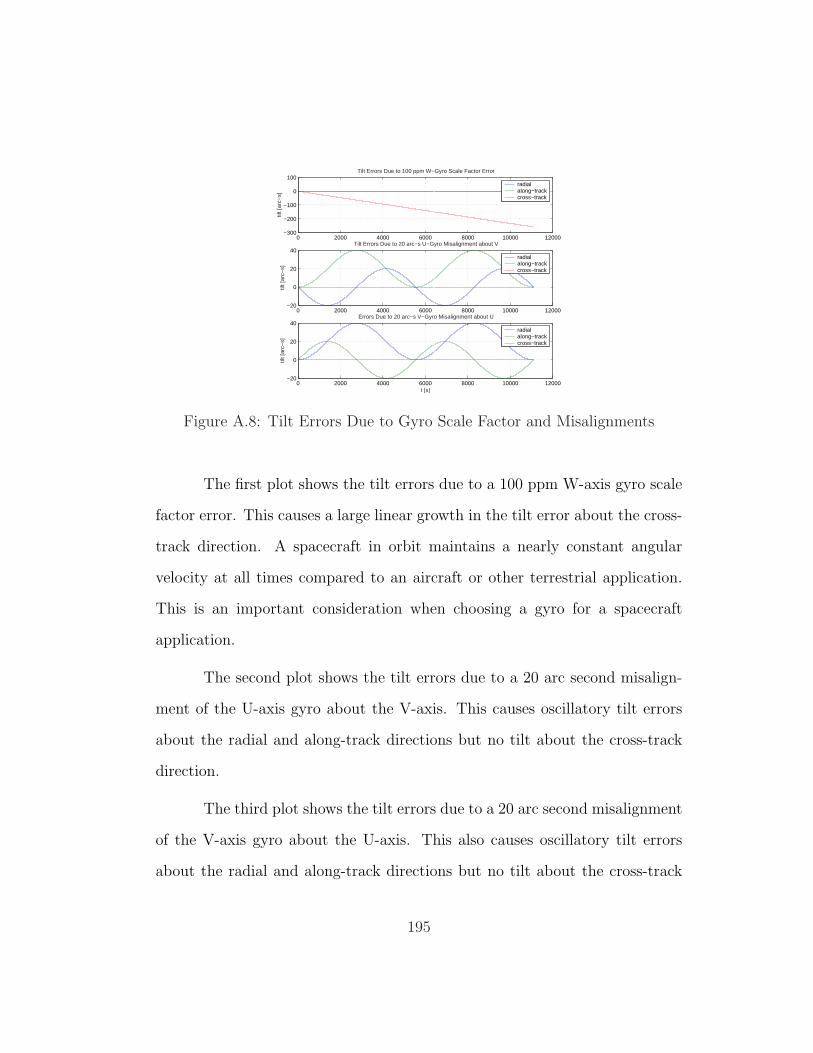
0 2000 4000 6000 8000 10000 12000−300

−200

−100

0

100

tilt [

arc−

s]

Tilt Errors Due to 100 ppm W−Gyro Scale Factor Error


0 2000 4000 6000 8000 10000 12000−20

0

20

40

tilt [

arc−

s]

Tilt Errors Due to 20 arc−s U−Gyro Misalignment about V


0 2000 4000 6000 8000 10000 12000−20

0

20

40

t [s]

tilt [

arc−

s]

Errors Due to 20 arc−s V−Gyro Misalignment about U


Figure A.8: Tilt Errors Due to Gyro Scale Factor and Misalignments

The first plot shows the tilt errors due to a 100 ppm W-axis gyro scale

factor error. This causes a large linear growth in the tilt error about the cross-

track direction. A spacecraft in orbit maintains a nearly constant angular

velocity at all times compared to an aircraft or other terrestrial application.

This is an important consideration when choosing a gyro for a spacecraft

application.

The second plot shows the tilt errors due to a 20 arc second misalign-

ment of the U-axis gyro about the V-axis. This causes oscillatory tilt errors

about the radial and along-track directions but no tilt about the cross-track

direction.

The third plot shows the tilt errors due to a 20 arc second misalignment

of the V-axis gyro about the U-axis. This also causes oscillatory tilt errors

about the radial and along-track directions but no tilt about the cross-track

195

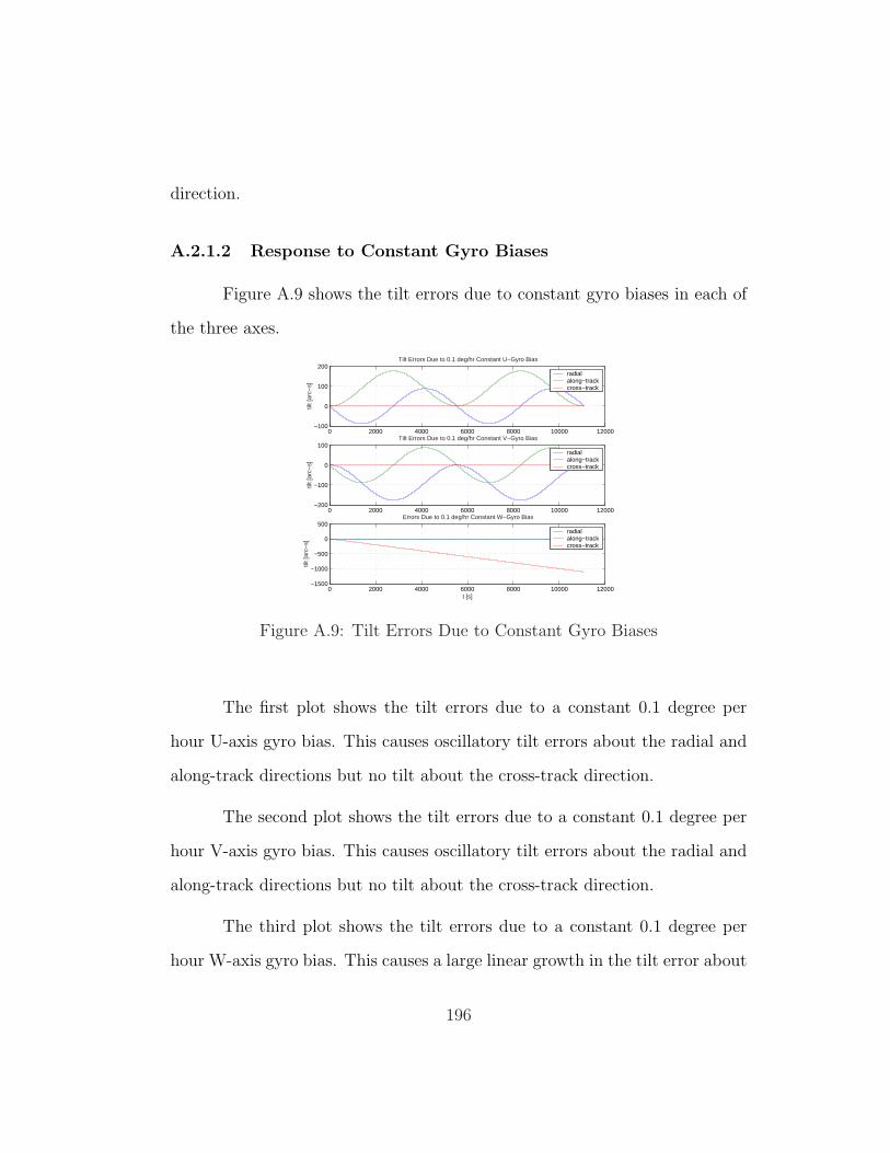
direction.

A.2.1.2 Response to Constant Gyro Biases

Figure A.9 shows the tilt errors due to constant gyro biases in each of

the three axes.

0 2000 4000 6000 8000 10000 12000−100

0

100

200

tilt [

arc−

s]

Tilt Errors Due to 0.1 deg/hr Constant U−Gyro Bias


0 2000 4000 6000 8000 10000 12000−200

−100

0

100

tilt [

arc−

s]

Tilt Errors Due to 0.1 deg/hr Constant V−Gyro Bias


0 2000 4000 6000 8000 10000 12000−1500

−1000

−500

0

500

t [s]

tilt [

arc−

s]

Errors Due to 0.1 deg/hr Constant W−Gyro Bias


Figure A.9: Tilt Errors Due to Constant Gyro Biases

The first plot shows the tilt errors due to a constant 0.1 degree per

hour U-axis gyro bias. This causes oscillatory tilt errors about the radial and

along-track directions but no tilt about the cross-track direction.

The second plot shows the tilt errors due to a constant 0.1 degree per

hour V-axis gyro bias. This causes oscillatory tilt errors about the radial and

along-track directions but no tilt about the cross-track direction.

The third plot shows the tilt errors due to a constant 0.1 degree per

hour W-axis gyro bias. This causes a large linear growth in the tilt error about

196

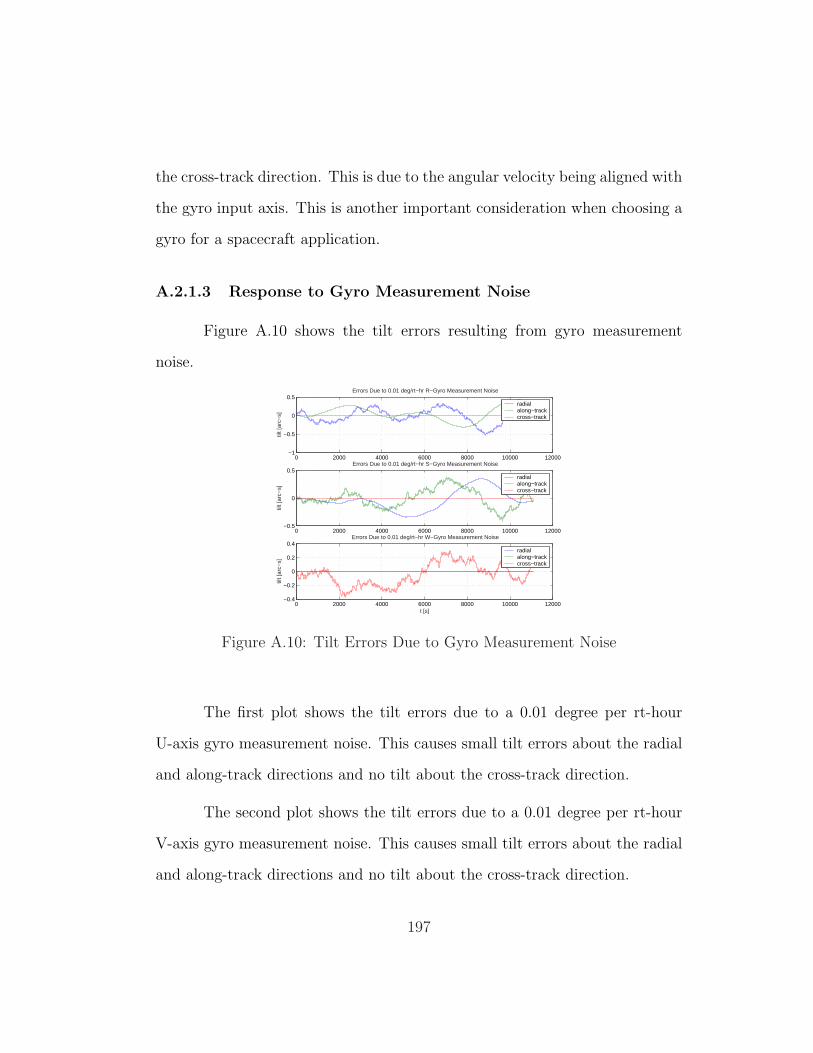
the cross-track direction. This is due to the angular velocity being aligned with

the gyro input axis. This is another important consideration when choosing a

gyro for a spacecraft application.

A.2.1.3 Response to Gyro Measurement Noise

Figure A.10 shows the tilt errors resulting from gyro measurement

noise.

0 2000 4000 6000 8000 10000 12000−1

−0.5

0

0.5

tilt [

arc−

s]

Errors Due to 0.01 deg/rt−hr R−Gyro Measurement Noise


0 2000 4000 6000 8000 10000 12000−0.5

0

0.5

tilt [

arc−

s]

Errors Due to 0.01 deg/rt−hr S−Gyro Measurement Noise


0 2000 4000 6000 8000 10000 12000−0.4

−0.2

0

0.2

0.4

t [s]

tilt [

arc−

s]

Errors Due to 0.01 deg/rt−hr W−Gyro Measurement Noise


Figure A.10: Tilt Errors Due to Gyro Measurement Noise

The first plot shows the tilt errors due to a 0.01 degree per rt-hour

U-axis gyro measurement noise. This causes small tilt errors about the radial

and along-track directions and no tilt about the cross-track direction.

The second plot shows the tilt errors due to a 0.01 degree per rt-hour

V-axis gyro measurement noise. This causes small tilt errors about the radial

and along-track directions and no tilt about the cross-track direction.

197

The third plot shows the tilt errors due to a 0.01 degree per rt-hour

W-axis gyro measurement noise. This causes small tilts about the cross-track

direction and no tilt errors about the radial or cross-track directions.

A.2.2 Constant Specific Force Cases

Accelerometer errors are only observable in the presence of specific

forces. In order to observe the position and velocity errors resulting from

imperfect gyros and accelerometers, a 100 µg constant specific force is applied

along one of the true UVW axes.

A.2.2.1 Response to Gyro Errors

The position and velocity errors due to imperfect gyros are presented

in this section. In each case, the platform tilt error caused by the gyro error

leads to an erroneous transformation of the specific force vector from the body

frame to the ECI frame, leading to increasing position and velocity errors.

Figure A.11 shows the errors due to a 100 ppm scale factor error in

the W-axis gyro when a constant specific force is applied in the along-track

direction. This causes a tilt about the cross-track direction which grows lin-

early with time. The tilt causes part of the along-track specific force to be

interpreted as a specific force in the radial direction. This causes position and

velocity errors in radial and along-track directions.

Figure A.12 shows the errors due to a 0.1 deg/hr constant bias in the W-

axis gyro when a constant specific force is applied in the along-track direction.

198

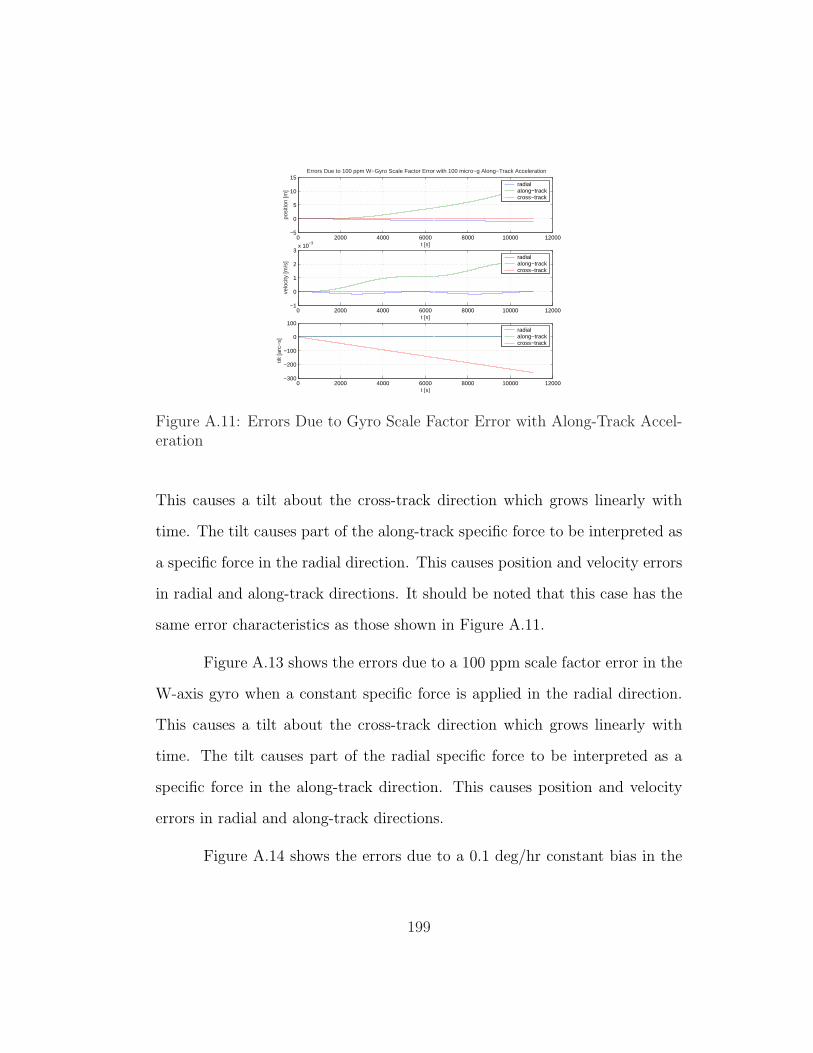
0 2000 4000 6000 8000 10000 12000−5

0

5

10

15

t [s]

posi

tion

[m]

Errors Due to 100 ppm W−Gyro Scale Factor Error with 100 micro−g Along−Track Acceleration


0 2000 4000 6000 8000 10000 12000−1

0

1

2

3x 10

−3

t [s]

velo

city

[m/s

]


0 2000 4000 6000 8000 10000 12000−300

−200

−100

0

100

t [s]

tilt [

arc−

s]


Figure A.11: Errors Due to Gyro Scale Factor Error with Along-Track Accel-eration

This causes a tilt about the cross-track direction which grows linearly with

time. The tilt causes part of the along-track specific force to be interpreted as

a specific force in the radial direction. This causes position and velocity errors

in radial and along-track directions. It should be noted that this case has the

same error characteristics as those shown in Figure A.11.

Figure A.13 shows the errors due to a 100 ppm scale factor error in the

W-axis gyro when a constant specific force is applied in the radial direction.


time. The tilt causes part of the radial specific force to be interpreted as a

specific force in the along-track direction. This causes position and velocity

errors in radial and along-track directions.

Figure A.14 shows the errors due to a 0.1 deg/hr constant bias in the

199

0 2000 4000 6000 8000 10000 12000−20

0

20

40

60

t [s]

posi

tion

[m]

Errors Due to 0.1 deg/hr Constant W−Gyro Bias with 100 micro−g Along−Track Acceleration


0 2000 4000 6000 8000 10000 12000−5

0

5

10x 10

−3

t [s]

velo

city

[m/s

]


0 2000 4000 6000 8000 10000 12000−1500

−1000

−500

0

500

t [s]

tilt [

arc−

s]


Figure A.12: Errors Due to Constant Gyro Bias with Along-Track Acceleration

W-axis gyro when a constant specific force is applied in the radial direction.


time. The tilt causes part of the radial specific force to be interpreted as a

specific force in the along-track direction. This causes position and velocity

errors in radial and along-track directions. It should be noted that this case

has the same error characteristics as those shown in Figure A.13.

Figure A.15 shows the errors due to a 20 arc-second misalignment of

the V-axis gyro about the U-axis when a constant specific force is applied

in the cross-track direction. This causes tilts about the radial and along-

track directions. The tilts cause part of the cross-track specific force to be

interpreted as a specific force in the radial and along-track directions. This

causes the position and velocity errors in the radial and along-track directions

as well as very small position and velocity errors in the cross-track direction,

200

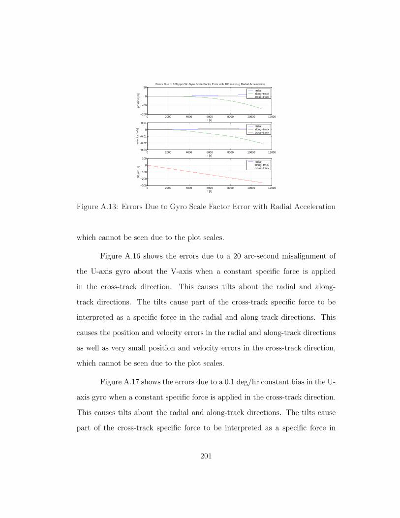
0 2000 4000 6000 8000 10000 12000−100

−50

0

50

t [s]

posi

tion

[m]

Errors Due to 100 ppm W−Gyro Scale Factor Error with 100 micro−g Radial Acceleration


0 2000 4000 6000 8000 10000 12000−0.03

−0.02

−0.01

0

0.01

t [s]

velo

city

[m/s

]


0 2000 4000 6000 8000 10000 12000−300

−200

−100

0

100

t [s]

tilt [

arc−

s]


Figure A.13: Errors Due to Gyro Scale Factor Error with Radial Acceleration

which cannot be seen due to the plot scales.

Figure A.16 shows the errors due to a 20 arc-second misalignment of

the U-axis gyro about the V-axis when a constant specific force is applied

in the cross-track direction. This causes tilts about the radial and along-

track directions. The tilts cause part of the cross-track specific force to be

interpreted as a specific force in the radial and along-track directions. This

causes the position and velocity errors in the radial and along-track directions

as well as very small position and velocity errors in the cross-track direction,

which cannot be seen due to the plot scales.

Figure A.17 shows the errors due to a 0.1 deg/hr constant bias in the U-

axis gyro when a constant specific force is applied in the cross-track direction.

This causes tilts about the radial and along-track directions. The tilts cause

part of the cross-track specific force to be interpreted as a specific force in

201

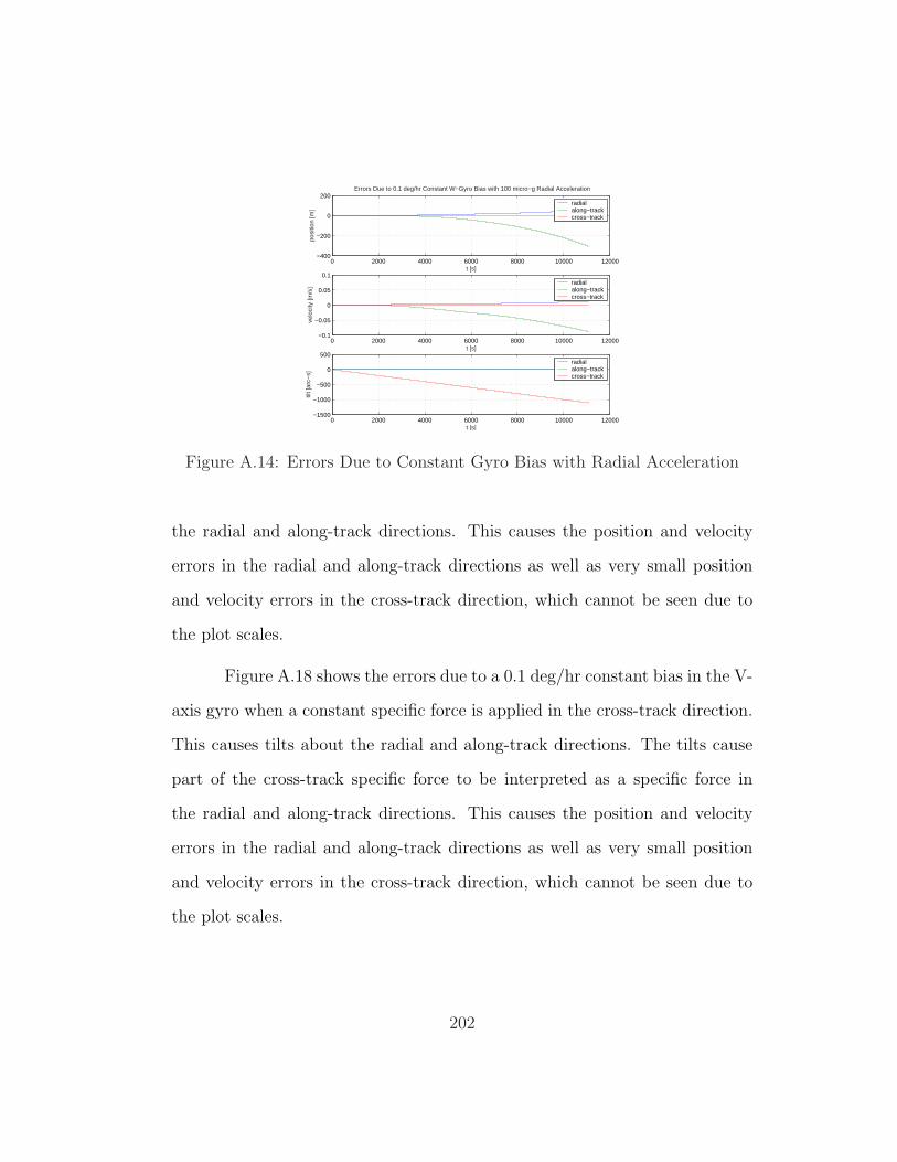
0 2000 4000 6000 8000 10000 12000−400

−200

0

200

t [s]

posi

tion

[m]

Errors Due to 0.1 deg/hr Constant W−Gyro Bias with 100 micro−g Radial Acceleration


0 2000 4000 6000 8000 10000 12000−0.1

−0.05

0

0.05

0.1

t [s]

velo

city

[m/s

]


0 2000 4000 6000 8000 10000 12000−1500

−1000

−500

0

500

t [s]

tilt [

arc−

s]


Figure A.14: Errors Due to Constant Gyro Bias with Radial Acceleration

the radial and along-track directions. This causes the position and velocity

errors in the radial and along-track directions as well as very small position

and velocity errors in the cross-track direction, which cannot be seen due to

the plot scales.

Figure A.18 shows the errors due to a 0.1 deg/hr constant bias in the V-

axis gyro when a constant specific force is applied in the cross-track direction.

This causes tilts about the radial and along-track directions. The tilts cause

part of the cross-track specific force to be interpreted as a specific force in

the radial and along-track directions. This causes the position and velocity

errors in the radial and along-track directions as well as very small position

and velocity errors in the cross-track direction, which cannot be seen due to

the plot scales.

202

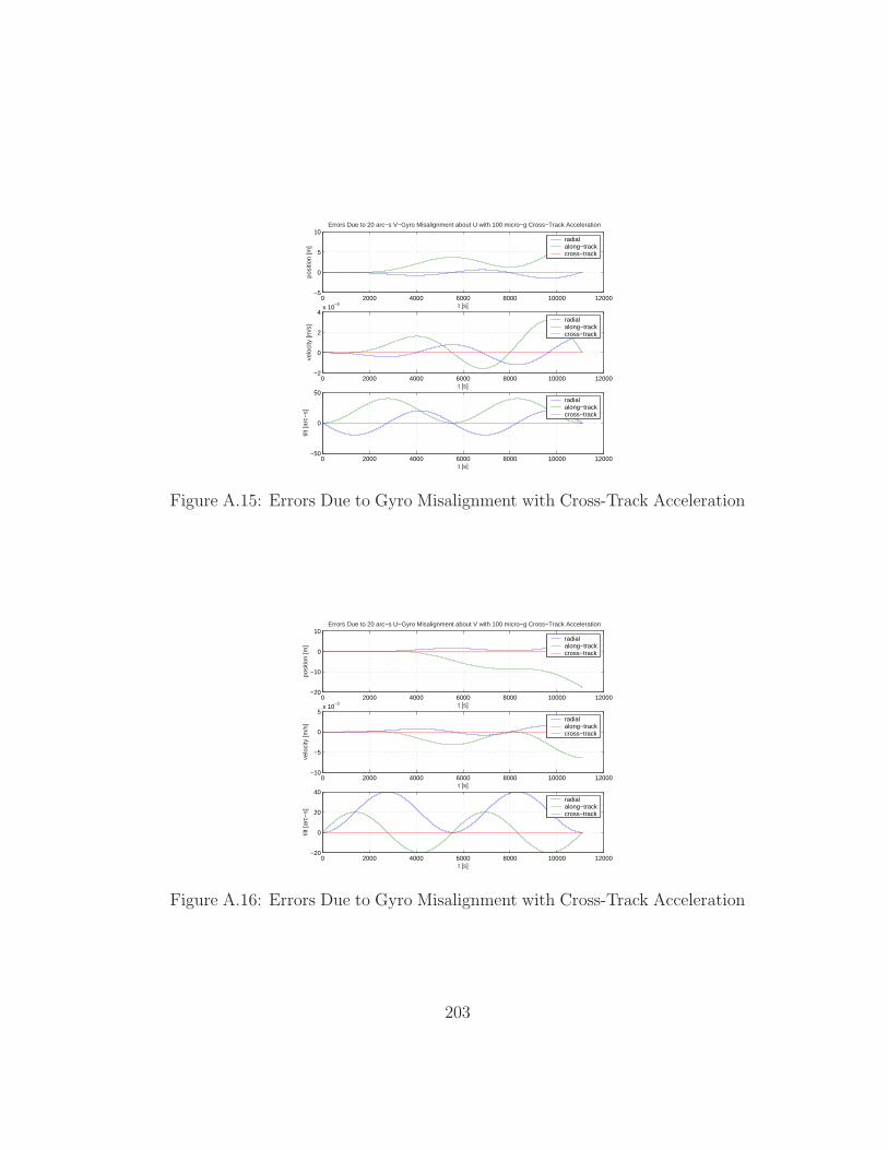
0 2000 4000 6000 8000 10000 12000−5

0

5

10

t [s]po

sitio

n [m

]

Errors Due to 20 arc−s V−Gyro Misalignment about U with 100 micro−g Cross−Track Acceleration


0 2000 4000 6000 8000 10000 12000−2

0

2

4x 10

−3

t [s]

velo

city

[m/s

]


0 2000 4000 6000 8000 10000 12000−50

0

50

t [s]

tilt [

arc−

s]


Figure A.15: Errors Due to Gyro Misalignment with Cross-Track Acceleration

0 2000 4000 6000 8000 10000 12000−20

−10

0

10

t [s]

posi

tion

[m]

Errors Due to 20 arc−s U−Gyro Misalignment about V with 100 micro−g Cross−Track Acceleration


0 2000 4000 6000 8000 10000 12000−10

−5

0

5x 10

−3

t [s]

velo

city

[m/s

]


0 2000 4000 6000 8000 10000 12000−20

0

20

40

t [s]

tilt [

arc−

s]


Figure A.16: Errors Due to Gyro Misalignment with Cross-Track Acceleration

203

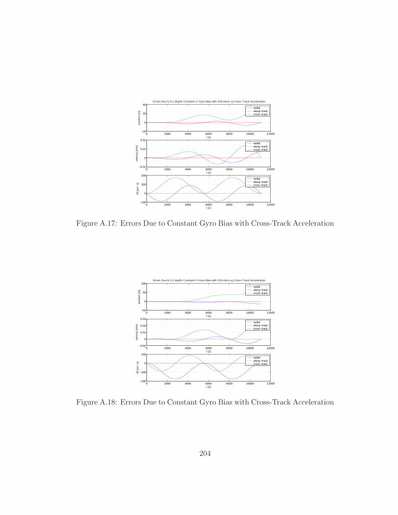
0 2000 4000 6000 8000 10000 12000−20

0

20

40

t [s]po

sitio

n [m

]

Errors Due to 0.1 deg/hr Constant U−Gyro Bias with 100 micro−g Cross−Track Acceleration


0 2000 4000 6000 8000 10000 12000−0.01

0

0.01

0.02

t [s]

velo

city

[m/s

]


0 2000 4000 6000 8000 10000 12000−100

0

100

200

t [s]

tilt [

arc−

s]


Figure A.17: Errors Due to Constant Gyro Bias with Cross-Track Acceleration

0 2000 4000 6000 8000 10000 12000−50

0

50

100

t [s]

posi

tion

[m]

Errors Due to 0.1 deg/hr Constant V−Gyro Bias with 100 micro−g Cross−Track Acceleration


0 2000 4000 6000 8000 10000 12000−0.01

0

0.01

0.02

0.03

t [s]

velo

city

[m/s

]


0 2000 4000 6000 8000 10000 12000−200

−100

0

100

t [s]

tilt [

arc−

s]


Figure A.18: Errors Due to Constant Gyro Bias with Cross-Track Acceleration

204

A.2.2.2 Response to Accelerometer Scale Factor Error

The navigation errors due to accelerometer scale factor errors are shown

in this section.

Figure A.19 shows the errors caused by a 350 ppm scale factor error

in the V-axis accelerometer when there is a constant specific force applied in

the along-track acceleration. The scale factor error causes the INS to mea-

sure less force than is actually being applied. Initially, this causes the actual

along-track velocity to be greater than the estimated along-track velocity. But

the along-track velocity error produces a radial velocity error due to the er-

ror in the estimation of semi-major axis. The semi-major axis of the actual

orbit increases faster than the estimated semi-major axis. After about 1000

seconds, the effects of underestimating the semi-major axis becomes dominant

and causes the estimated along-track velocity to exceed the actual along-track

velocity.

Figure A.20 shows the errors caused by a 350 ppm scale factor error

in the U-axis accelerometer when there is a constant specific force applied in

the radial acceleration. The scale factor error causes the INS to measure less

force than is actually being applied. After a complete orbit period, this error

produces no net radial position error because a each point in the orbit, the

erroneous force measurement has been cancelled out by the erroneous force

measured at a point 180 degrees in true anomaly away. This is indicated by

the radial velocity error which is a sine wave centered on zero whose period

is equal to one orbit period. However, during the course of an orbit period,

205

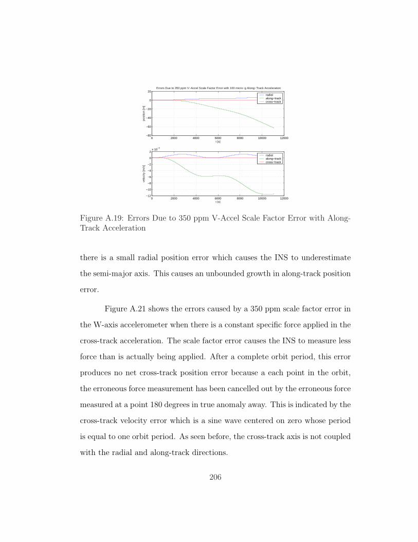
0 2000 4000 6000 8000 10000 12000−80

−60

−40

−20

0

20

t [s]po

sitio

n [m

]

Errors Due to 350 ppm V−Accel Scale Factor Error with 100 micro−g Along−Track Acceleration


0 2000 4000 6000 8000 10000 12000−12

−10

−8

−6

−4

−2

0

2x 10

−3

t [s]

velo

city

[m/s

]


Figure A.19: Errors Due to 350 ppm V-Accel Scale Factor Error with Along-Track Acceleration

there is a small radial position error which causes the INS to underestimate

the semi-major axis. This causes an unbounded growth in along-track position

error.

Figure A.21 shows the errors caused by a 350 ppm scale factor error in

the W-axis accelerometer when there is a constant specific force applied in the

cross-track acceleration. The scale factor error causes the INS to measure less

force than is actually being applied. After a complete orbit period, this error

produces no net cross-track position error because a each point in the orbit,

the erroneous force measurement has been cancelled out by the erroneous force

measured at a point 180 degrees in true anomaly away. This is indicated by the

cross-track velocity error which is a sine wave centered on zero whose period

is equal to one orbit period. As seen before, the cross-track axis is not coupled

with the radial and along-track directions.

206

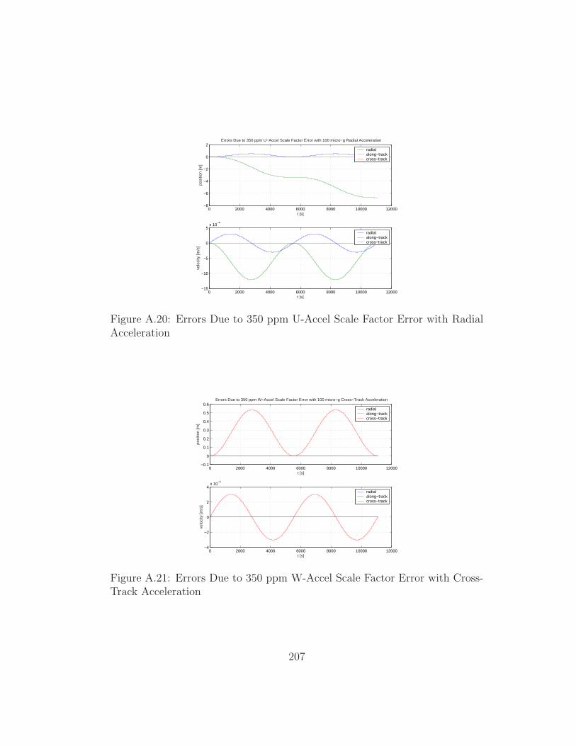
0 2000 4000 6000 8000 10000 12000−8

−6

−4

−2

0

2

t [s]

posi

tion

[m]

Errors Due to 350 ppm U−Accel Scale Factor Error with 100 micro−g Radial Acceleration


0 2000 4000 6000 8000 10000 12000−15

−10

−5

0

5x 10

−4

t [s]

velo

city

[m/s

]


Figure A.20: Errors Due to 350 ppm U-Accel Scale Factor Error with RadialAcceleration

0 2000 4000 6000 8000 10000 12000−0.1

0

0.1

0.2

0.3

0.4

0.5

0.6

t [s]

posi

tion

[m]

Errors Due to 350 ppm W−Accel Scale Factor Error with 100 micro−g Cross−Track Acceleration


0 2000 4000 6000 8000 10000 12000−4

−2

0

2

4x 10

−4

t [s]

velo

city

[m/s

]


Figure A.21: Errors Due to 350 ppm W-Accel Scale Factor Error with Cross-Track Acceleration

207

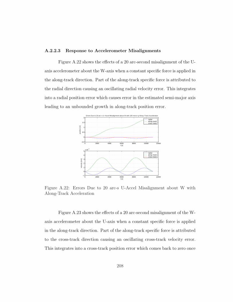
A.2.2.3 Response to Accelerometer Misalignments

Figure A.22 shows the effects of a 20 arc-second misalignment of the U-

axis accelerometer about the W-axis when a constant specific force is applied in

the along-track direction. Part of the along-track specific force is attributed to

the radial direction causing an oscillating radial velocity error. This integrates

into a radial position error which causes error in the estimated semi-major axis

leading to an unbounded growth in along-track position error.

0 2000 4000 6000 8000 10000 12000−0.5

0

0.5

1

1.5

2

t [s]

posi

tion

[m]

Errors Due to 20 arc−s U−Accel Misalignment about W with 100 micro−g Along−Track Acceleration


0 2000 4000 6000 8000 10000 12000−1

0

1

2

3

4

5x 10

−4

t [s]

velo

city

[m/s

]


Figure A.22: Errors Due to 20 arc-s U-Accel Misalignment about W withAlong-Track Acceleration

Figure A.23 shows the effects of a 20 arc-second misalignment of the W-

axis accelerometer about the U-axis when a constant specific force is applied

in the along-track direction. Part of the along-track specific force is attributed

to the cross-track direction causing an oscillating cross-track velocity error.

This integrates into a cross-track position error which comes back to zero once

208

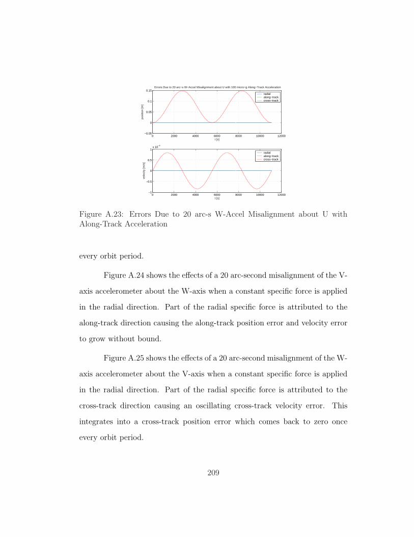
0 2000 4000 6000 8000 10000 12000−0.05

0

0.05

0.1

0.15

t [s]po

sitio

n [m

]

Errors Due to 20 arc−s W−Accel Misalignment about U with 100 micro−g Along−Track Acceleration


0 2000 4000 6000 8000 10000 12000−1

−0.5

0

0.5

1x 10

−4

t [s]

velo

city

[m/s

]


Figure A.23: Errors Due to 20 arc-s W-Accel Misalignment about U withAlong-Track Acceleration

every orbit period.

Figure A.24 shows the effects of a 20 arc-second misalignment of the V-

axis accelerometer about the W-axis when a constant specific force is applied

in the radial direction. Part of the radial specific force is attributed to the

along-track direction causing the along-track position error and velocity error

to grow without bound.

Figure A.25 shows the effects of a 20 arc-second misalignment of the W-

axis accelerometer about the V-axis when a constant specific force is applied

in the radial direction. Part of the radial specific force is attributed to the

cross-track direction causing an oscillating cross-track velocity error. This

integrates into a cross-track position error which comes back to zero once

every orbit period.

209

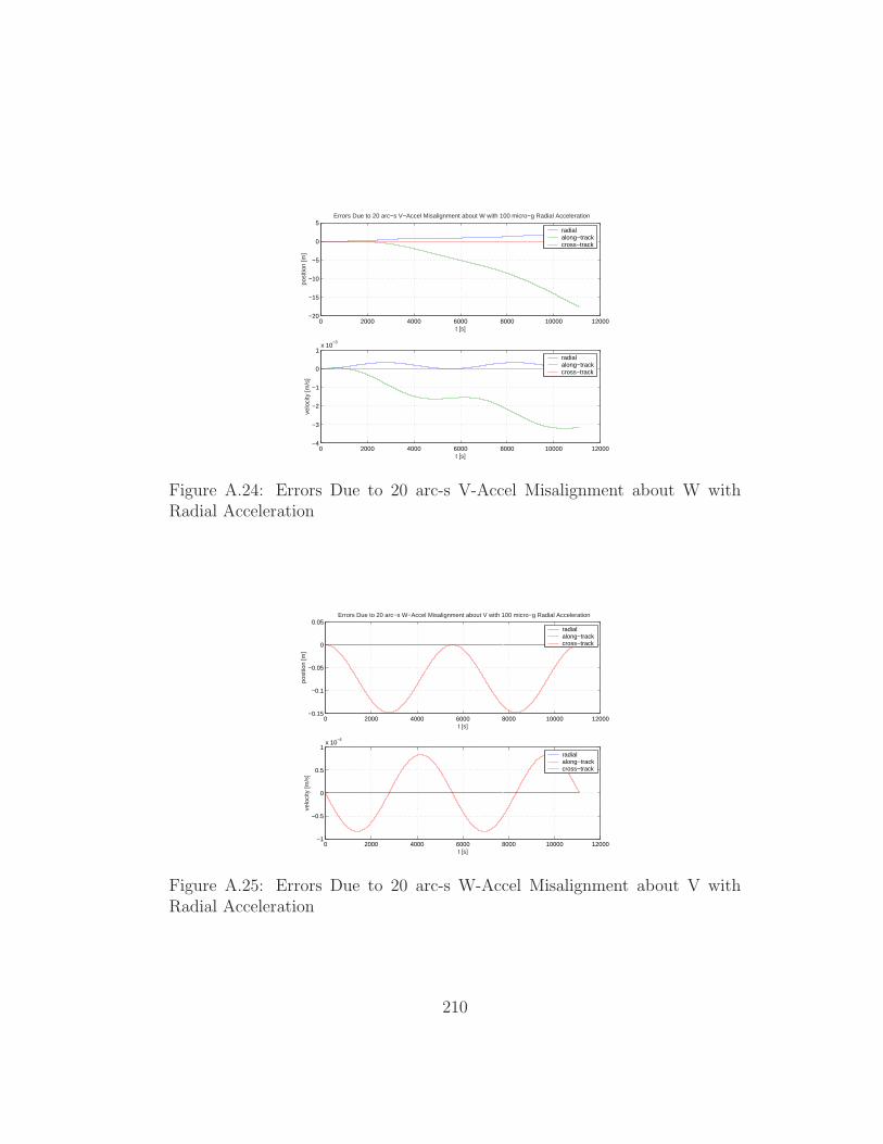
0 2000 4000 6000 8000 10000 12000−20

−15

−10

−5

0

5

t [s]

posi

tion

[m]

Errors Due to 20 arc−s V−Accel Misalignment about W with 100 micro−g Radial Acceleration


0 2000 4000 6000 8000 10000 12000−4

−3

−2

−1

0

1x 10

−3

t [s]

velo

city

[m/s

]


Figure A.24: Errors Due to 20 arc-s V-Accel Misalignment about W withRadial Acceleration

0 2000 4000 6000 8000 10000 12000−0.15

−0.1

−0.05

0

0.05

t [s]

posi

tion

[m]

Errors Due to 20 arc−s W−Accel Misalignment about V with 100 micro−g Radial Acceleration


0 2000 4000 6000 8000 10000 12000−1

−0.5

0

0.5

1x 10

−4

t [s]

velo

city

[m/s

]


Figure A.25: Errors Due to 20 arc-s W-Accel Misalignment about V withRadial Acceleration

210

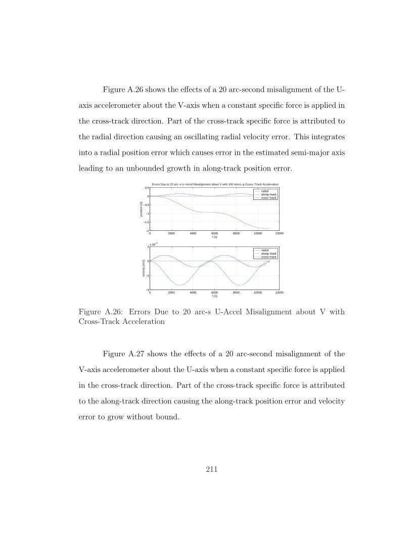
Figure A.26 shows the effects of a 20 arc-second misalignment of the U-

axis accelerometer about the V-axis when a constant specific force is applied in

the cross-track direction. Part of the cross-track specific force is attributed to

the radial direction causing an oscillating radial velocity error. This integrates

into a radial position error which causes error in the estimated semi-major axis

leading to an unbounded growth in along-track position error.

0 2000 4000 6000 8000 10000 12000−2

−1.5

−1

−0.5

0

0.5

t [s]

posi

tion

[m]

Errors Due to 20 arc−s U−Accel Misalignment about V with 100 micro−g Cross−Track Acceleration


0 2000 4000 6000 8000 10000 12000−4

−2

0

2x 10

−4

t [s]

velo

city

[m/s

]


Figure A.26: Errors Due to 20 arc-s U-Accel Misalignment about V withCross-Track Acceleration

Figure A.27 shows the effects of a 20 arc-second misalignment of the

V-axis accelerometer about the U-axis when a constant specific force is applied

in the cross-track direction. Part of the cross-track specific force is attributed

to the along-track direction causing the along-track position error and velocity

error to grow without bound.

211

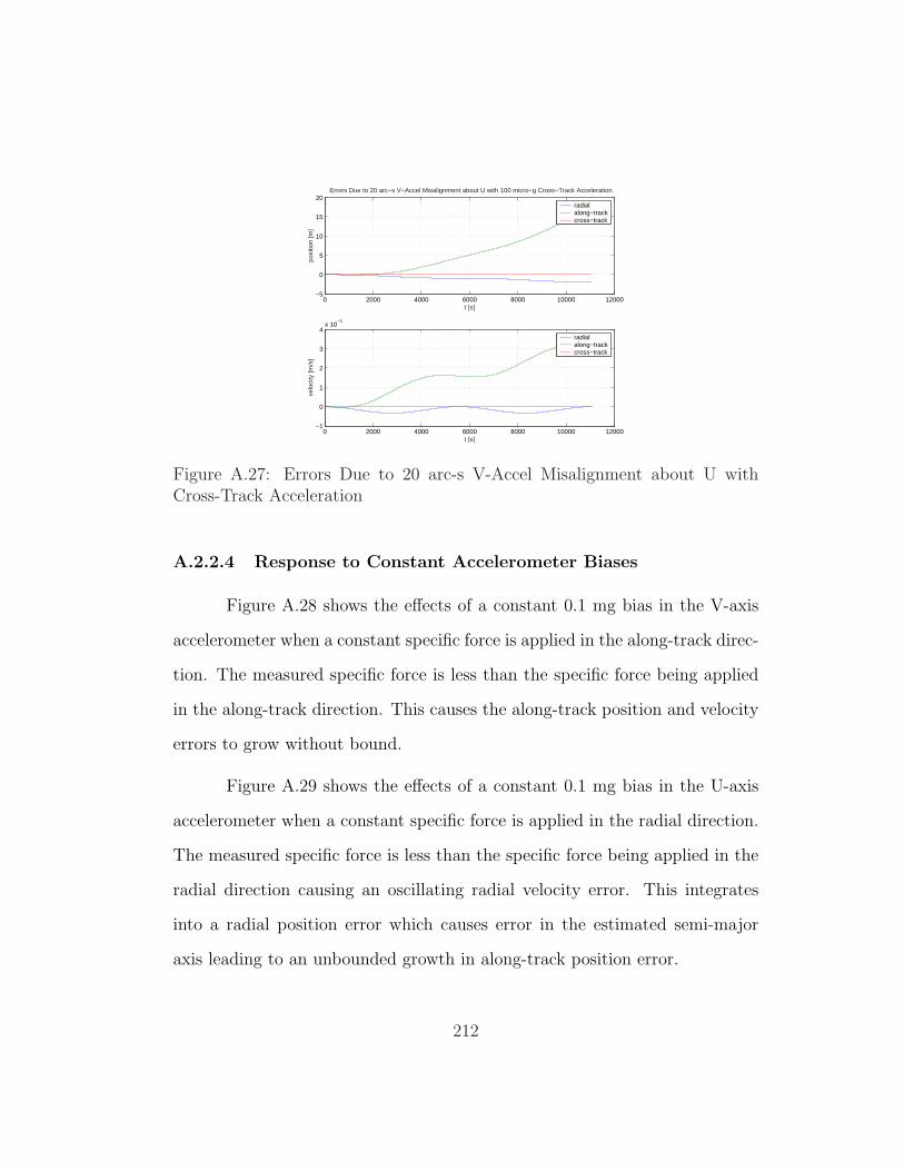
0 2000 4000 6000 8000 10000 12000−5

0

5

10

15

20

t [s]po

sitio

n [m

]

Errors Due to 20 arc−s V−Accel Misalignment about U with 100 micro−g Cross−Track Acceleration


0 2000 4000 6000 8000 10000 12000−1

0

1

2

3

4x 10

−3

t [s]

velo

city

[m/s

]


Figure A.27: Errors Due to 20 arc-s V-Accel Misalignment about U withCross-Track Acceleration

A.2.2.4 Response to Constant Accelerometer Biases

Figure A.28 shows the effects of a constant 0.1 mg bias in the V-axis

accelerometer when a constant specific force is applied in the along-track direc-

tion. The measured specific force is less than the specific force being applied

in the along-track direction. This causes the along-track position and velocity

errors to grow without bound.

Figure A.29 shows the effects of a constant 0.1 mg bias in the U-axis

accelerometer when a constant specific force is applied in the radial direction.

The measured specific force is less than the specific force being applied in the

radial direction causing an oscillating radial velocity error. This integrates

into a radial position error which causes error in the estimated semi-major

axis leading to an unbounded growth in along-track position error.

212

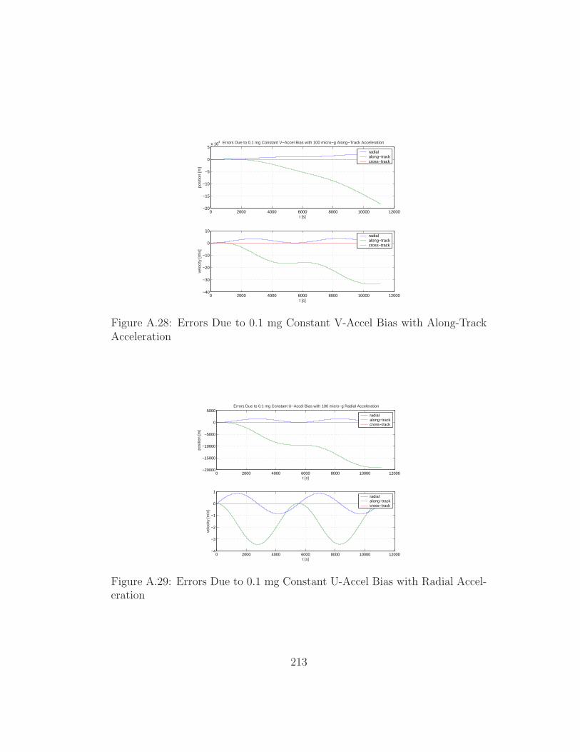
0 2000 4000 6000 8000 10000 12000−20

−15

−10

−5

0

5x 10

4

t [s]

posi

tion

[m]

Errors Due to 0.1 mg Constant V−Accel Bias with 100 micro−g Along−Track Acceleration


0 2000 4000 6000 8000 10000 12000−40

−30

−20

−10

0

10

t [s]

velo

city

[m/s

]


Figure A.28: Errors Due to 0.1 mg Constant V-Accel Bias with Along-TrackAcceleration

0 2000 4000 6000 8000 10000 12000−20000

−15000

−10000

−5000

0

5000

t [s]

posi

tion

[m]

Errors Due to 0.1 mg Constant U−Accel Bias with 100 micro−g Radial Acceleration


0 2000 4000 6000 8000 10000 12000−4

−3

−2

−1

0

1

t [s]

velo

city

[m/s

]


Figure A.29: Errors Due to 0.1 mg Constant U-Accel Bias with Radial Accel-eration

213

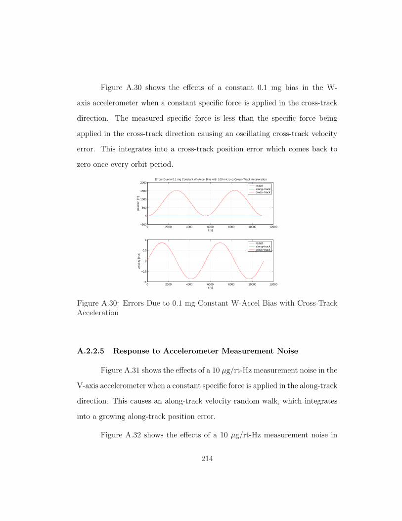
Figure A.30 shows the effects of a constant 0.1 mg bias in the W-

axis accelerometer when a constant specific force is applied in the cross-track

direction. The measured specific force is less than the specific force being

applied in the cross-track direction causing an oscillating cross-track velocity

error. This integrates into a cross-track position error which comes back to

zero once every orbit period.

0 2000 4000 6000 8000 10000 12000−500

0

500

1000

1500

2000

t [s]

posi

tion

[m]

Errors Due to 0.1 mg Constant W−Accel Bias with 100 micro−g Cross−Track Acceleration


0 2000 4000 6000 8000 10000 12000−1

−0.5

0

0.5

1

t [s]

velo

city

[m/s

]


Figure A.30: Errors Due to 0.1 mg Constant W-Accel Bias with Cross-TrackAcceleration

A.2.2.5 Response to Accelerometer Measurement Noise

Figure A.31 shows the effects of a 10 µg/rt-Hz measurement noise in the

V-axis accelerometer when a constant specific force is applied in the along-track

direction. This causes an along-track velocity random walk, which integrates

into a growing along-track position error.

Figure A.32 shows the effects of a 10 µg/rt-Hz measurement noise in

214

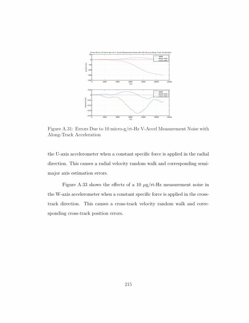
0 2000 4000 6000 8000 10000 12000−200

−150

−100

−50

0

50

t [s]po

sitio

n [m

]

Errors Due to 10 micro−g/rt−Hz V−Accel Measurement Noise with 100 micro−g Along−Track Acceleration


0 2000 4000 6000 8000 10000 12000−0.04

−0.03

−0.02

−0.01

0

0.01

t [s]

velo

city

[m/s

]


Figure A.31: Errors Due to 10 micro-g/rt-Hz V-Accel Measurement Noise withAlong-Track Acceleration

the U-axis accelerometer when a constant specific force is applied in the radial

direction. This causes a radial velocity random walk and corresponding semi-

major axis estimation errors.

Figure A.33 shows the effects of a 10 µg/rt-Hz measurement noise in

the W-axis accelerometer when a constant specific force is applied in the cross-

track direction. This causes a cross-track velocity random walk and corre-

sponding cross-track position errors.

215

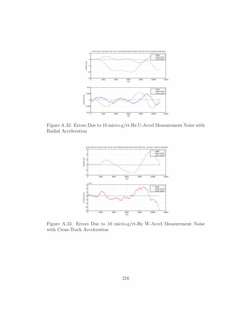
0 2000 4000 6000 8000 10000 12000−15

−10

−5

0

5

t [s]

posi

tion

[m]

Errors Due to 10 micro−g/rt−Hz U−Accel Measurement Noise with 100 micro−g Radial Acceleration


0 2000 4000 6000 8000 10000 12000−0.01

−0.005

0

0.005

0.01

t [s]

velo

city

[m/s

]


Figure A.32: Errors Due to 10 micro-g/rt-Hz U-Accel Measurement Noise withRadial Acceleration

0 2000 4000 6000 8000 10000 12000−4

−2

0

2

4

6

t [s]

posi

tion

[m]

Errors Due to 10 micro−g/rt−Hz W−Accel Measurement Noise with 100 micro−g Cross−Track Acceleration


0 2000 4000 6000 8000 10000 12000−8

−6

−4

−2

0

2

4

6x 10

−3

t [s]

velo

city

[m/s

]


Figure A.33: Errors Due to 10 micro-g/rt-Hz W-Accel Measurement Noisewith Cross-Track Acceleration

216

A.3 Conclusions

A linear INS error model for a spacecraft in orbit has been developed.

This error model was used to construct an orbital INS error simulator, which

computes the navigation and attitude errors committed by an unaided INS in

orbit. The following conclusions about unaided INS navigation can be drawn

from the simulation results:

1. The unforced errors behave according to the CW equations.

2. The Schuler period = the orbit period.

3. Initial radial position errors and along-track velocity errors cause un-

bounded position error growth. This is equivalent to an initial error in

the estimate of semi-major axis.

4. Radial and along-track errors are coupled because they both affect the

energy or semi-major axis of the estimated orbit.

5. Errors in the estimation of the semi-major axis lead to unbounded error

growth. Therefore, the ability to accurately estimate the semi-major

axis should be a key figure of merit for evaluating a spacecraft INS.

6. Cross-track errors are not coupled with the along-track or radial errors.

7. Unforced platform tilts are constant in inertial space.

217

8. Spacecraft have a constant, high angular rate due to orbital motion,

therefore an INS in orbit is sensitive to gyro scale factor and bias errors

about the angular momentum vector.

9. Unbounded along-track position errors result from: along-track accelerom-

eter scale factor or bias errors with along-track specific force, radial ac-

celerometer scale factor or bias errors with radial specific force, mis-

alignment of radial accelerometer with along-track or cross-track spe-

cific force, and misalignment of along-track accelerometer with radial or

cross-track specific force.

218

Appendix B

Stochastic Process Models

Maybeck [29] provides an excellent discussion of stochastic process mod-

els, which is summarized briefly in this section. The following stochastic pro-

cesses are used in INS error models: white Gaussian noise, Gaussian random

constants, random walks and first order Markov processes, whose characteris-

tics are described below.

B.1 White Gaussian Noise

A process x (· , ·) is a white Gaussian process if, for any choice of N

times, the N random vectors x (t1, ·) , . . . ,x (tN , ·) are independent Gaussian

random vectors. This implies:

Ex (ti)x

T (tj)

= Ψxx (ti) δ (ti − tj) (B.1)

B.2 Gaussian Random Constant

A random constant is modelled as a Gaussian random constant x (t0)

with a specified mean m0 and covariance P0 that behaves according to:

x (t) = 0 (B.2)

219

This model is used for bias stability for gyros and accelerometers, scale

factor errors and misalignments. The value can vary from one turn-on to the

next but remains constant while the instrument is turned on.

B.3 Random Walk

Random walk is the output generated by integrating white Gaussian

noise. If w (t)is zero-mean, white Gaussian noise process then:

x (t) = w (t) ; x (t0) ≡ 0 (B.3)

where E w (t) w (t + τ) = Qδ (τ) and E x2 (t) = Q [t− t0].

B.4 First Order Markov

A first order Markov process is a first order lag driven by zero-mean

white Gaussian noise of strength Q described by:

x (t) = − 1

Tx (t) + w (t) (B.4)

where E [x (t) x (t + τ)] = σ2e− |τ |/T and Q = 2σ2

/T .

B.5 Equivalent Discrete-Time Models

The implementation of stochastic process models on a digital computer

necessitates the development of discrete-time models that are equivalent to

the continuous-time models. This development presented in Maybeck [29] is

summarized below.

220

The general continuous-time differential equation is given by

x (t) = F (t)x (t) + B (t)u (t) + G (t)w (t) (B.5)

where u(t) is a vector of deterministic controls (or forcing functions) applied

at time t and w(t) is a zero-mean, white Gaussian noise vector of strength

Q(t). If u(t) is held constant over each sample period from sample time ti to

ti+1, at time ti+1, the solution to equation (B.5) can be written as:

x (ti+1) = Φ (ti+1, ti)x (ti) +[∫ ti+1

tiΦ (ti+1, τ)B (τ) dτ

]u (ti)

+[∫ ti+1

tiΦ (ti+1, τ)G (τ) dβ (τ)

] (B.6)

This can be written as an equivalent stochastic difference equation as:

x (ti+1) = Φ (ti+1, ti)x (ti) + Bd (ti)u (ti) + wd (ti) (B.7)

where:

Bd (ti) =

∫ ti+1

ti

Φ (ti+1, τ)B (τ) dτ (B.8)

and wd (ti) is a white Gaussian discrete-time stochastic process whose statistics

are equal to those of∫ ti+1

tiΦ (ti+1, τ)G (τ) dβ (τ) for all sample times, hence:

E wd (ti) = 0 (B.9)

Ewd (ti)w

Td (ti)

= Qd (B.10)

Qd =

∫ ti+1

ti

Φ (ti+1, τ)G (τ)Q (τ)GT (τ) ΦT (ti+1, τ) dτ (B.11)

Ewd (ti)w

Td (tj)

= 0 (B.12)

221

In the case of a time-invariant system with stationary noise inputs, and

a sample period that is short compared to the system’s natural transients, the

following first order approximations may be used:

Φ (ti+1, ti) ≈ I + F (ti) [ti+1 − ti] (B.13)

Bd (ti) ≈ B (ti) [ti+1 − ti] (B.14)

Qd (ti) ≈ G (ti)Q (ti) GT (ti) [ti+1 − ti] (B.15)

B.5.1 First Order Markov

For a scalar, first order Markov process with a fixed time interval be-

tween samples ∆t:

Φ (ti+1, ti) = e−1T

∆t; G = 1; Q =2σ2

T(B.16)

Substituting (B.16) into (B.11) leads to:

Qd = Q

∫ ti+1

ti

e−2T

(ti+1−τ)dτ =QT

2

[1− e−

2T

∆t]

= σ2[1− e−

2T

∆t]

(B.17)

B.5.2 Random Walk

For a random walk process with a fixed time interval between samples:

Φ (ti+1, ti) = 1; G = 1 (B.18)

therefore,

Qd = Q ∆t (B.19)

222

Bibliography

[1] Penina Axelrad, Christopher J. Comp, and Peter F. MacDoran. SNR-

Based Multipath Error Correction for GPS Differential Phase. IEEE

Transactions on Aerospace and Electronic Systems, 32(2), April 1996.

[2] B. Belloul, S.R. Saunders, M.A.N. Parks, and B.G. Evans. Measurement

and Modelling of Wideband Propagation at L- and S-bands Applicable to

the LMS Channel. IEEE Proceedings: Microwave Antenna Propagation,

147(2), April 2000.

[3] Donald O. Benson. A Comparison of Two Approaches to Pure-Inertial

and Doppler-Inertial Error Analysis. IEEE Transactions on Aerospace

and Electronic Systems, AES-11(4):447–455, July 1975.

[4] Michael S. Braasch. On the Characterization of Multipath Errors in

Satellite-Based Precision Approach and Landing Systems. PhD thesis,

Ohio University, June 1992.

[5] Kevin Braden, Clint Browning, and Hendrik Gelderloos. Integrated Iner-

tial Navigation System/Global Positioning System (INS/GPS) for Auto-

matic Space Return Vehicle. Proceedings of the IEEE/AIAA/NASA 9th

Digital Avionics Systems Conference, October 1990.

223

[6] Kenneth R. Britting. Inertial Navigation Systems Analysis. John Wiley

& Sons, Inc., New York, 1971.

[7] Robert Grover Brown and Patrick Y.C. Hwang. Introduction to Random

Signals and Applied Kalman Filtering. John Wiley & Sons, New York,

3rd edition, 1997.

[8] NASA Marshall Spaceflight Center. Beginning a New Era of Space Flight:

The Orbital Space Plane. NASA Fact Sheets, (FS-2003-05-64-MSFC),

May 2003.

[9] NASA Marshall Spaceflight Center. The Space Launch Initiative: Tech-

nology to Pioneer the Space Frontier. NASA Fact Sheets, (FS-2003-02-

28-MSFC), February 2003.

[10] Averil B. Chatfield. Fundamentals of High Accuracy Inertial Naviga-

tion. American Institute of Aeronautics and Astronautics, Inc., Reston,

Virginia, 1997.

[11] Christopher J. Comp. GPS Carrier Phase Multipath Characterization

and a Mitigation Technique Using the Signal-To-Noise Ratio. PhD thesis,

University of Colorado, July 1996.

[12] Timothy P. Crain and Robert H. Bishop. Mars Entry Navigation: Atmo-

spheric Interface Through Parachute Deploy. Proceedings of the AIAA

Atmospheric Flight Mechanics Conference, (AIAA Paper 2002-4501), Au-

gust 2002.

224

[13] Takuji Ebinuma. Precision Spacecraft Rendezvous Using Global Posi-

tioning System: An Integrated Hardware Approach. PhD thesis, The

University of Texas at Austin, August 2001.

[14] Joseph Elchynski, Jeff Kirkland, and Jim Conner. Development and

Test Results of a Precision Approach and Landing Capability for Military

Aircraft Using an Embedded GPS/INS (EGI) System. Proceedings of

IEEE Position Location and Navigation Symposium.

[15] Jay A. Farrell and Matthew Barth. The Global Positioning System and

Inertial Navigation. McGraw-Hill, New York, 1999.

[16] Bernard Friedland. Analysis of Strapdown Navigation Using Quater-

nions. IEEE Transactions on Aerospace and Electronic Systems, AES-

14(5):764–768, September 1978.

[17] Susan F. Gomez. Flying High: GPS on the International Space Station

and Crew Return Vehicle. GPS World, June 2002.

[18] John L. Goodman. Space Shuttle Navigation in the GPS Era. Proceed-

ings of the ION National Technical Meeting, January 2001.

[19] John L. Goodman. GPS in Earth Orbit - Experiences from the Space

Shuttle, International Space Station and Crew Return Vehicle Programs.

Proceedings of the Core Technologies for Space Systems Conference, Novem-

ber 2002. Available at: http://www.spacecoretech.org/.

225

[20] Hari B. Hablani, Myron L. Tapper, and David J. Dana-Bashian. Guid-

ance and Relative Navigation for Autonomous Rendezvous in a Circular

Orbit. Journal of Guidance, Control, and Dynamics, 25(3), May - June

2002.

[21] Bernhard Hoffman-Wellenhof, Herbert Lichtenegger, and James Collins.

Global Positioning System: Theory and Practice. Springer-Verlag/Wien,

New York, 5th edition, 2001.

[22] Christopher Jekeli. Inertial Navigations Systems with Geodetic Applica-

tions. Walter de Gruyter GmbH & Co., Berlin, Germany, 2000.

[23] Elliott D. (ed.) Kaplan. Understanding GPS: Principles and Applica-

tions. Artech House Publishers, Norwood, MA, 1996.

[24] Karl Kovach. New User Equivalent Range Error (UERE) Budget for the

Modernized Navstar Global Positioning System (GPS). Proceedings of

the ION National Technical Meeting, January 2000.

[25] William C.Y. Lee. Mobile Communications Design Fundamentals. Howard

W. Sams & Co., Indianapolis, IN, 1986.

[26] E. Glenn Lightsey. Development and Flight Demonstration of a GPS

Receiver for Space. PhD thesis, Stanford University, February 1997.

[27] E. Glenn Lightsey and Jaeyong Um. Autonomous Relative Navigation

Methods in the Proximity of the International Space Station. Proceedings

of the KIS-2001 Conference.

226

[28] Cheng-Hsien Liu and et al. Characterization of a High-Sensitivity Mi-

cromachined Tunneling Accelerometer with Micro-g Resolution. Journal

of Micromechanical Systems, 7(2), June 1998.

[29] Peter S. Maybeck. Stochastic Models, Estimation, and Control, volume 1.

Academic Press, Inc., Florida, 1997.

[30] Oliver Montenbruck and Eberhard Gill. Satellite Orbits: Models, Meth-

ods, and Applications. Springer-Verlag, Berlin, Germany, 2000.

[31] Emilio Mora-Castro, Carmelo Carrascosa-Sanz, and Guillermo Ortega.

Characterisation of the Multipath Effects on the GPS Pseudorange and

Carrier Phase Measurements. Proceedings of the ION-GPS 1998 Confer-

ence, 1998.

[32] NASA. Introduction to NASA’s Integrated Space Transportation Plan

and Space Launch Initiative. May 2001. http:\\www.nasa.gov.

[33] GPS Program Office. NAVSTAR GPS Space Segment/Navigation User

Interfaces. Technical Report ICD-GPS-200, ARINC Research Corp.,

Fountain Valley, CA, 1997.

[34] Bradford W. Parkinson and James J. Spilker, Jr, editors. Global Posi-

tioning System: Theory and Applications, volume 1 of Progress in Astro-

nautics and Aeronautics. American Institute of Aeronautics and Astro-

nautics, Inc., Washington, DC, 1996.

[35] J.G. Proakis. Digital Communications. Wiley & Sons, New York, 1989.

227

[36] Theodore S. Rappaport. Wireless Communications: Principles and Prac-

tice. Prentice-Hall, Inc., Upper Saddle River, NJ, 2nd edition, 2002.

[37] Terry V. Roszhart, Hal Jerman, Joe Drake, and Constant de Cotiis. An

Inertial-Grade, Micromachined Vibrating Beam Accelerometer. Proceed-

ings of Transducers ’95, June 1995.

[38] Adel A. M. Saleh and Reinaldo A. Valenzuela. A Statistical Model for

Indoor Multipath Propagation. IEEE Journal on Selected Areas in Com-

munications, SAC-5(2), February 1987.

[39] S.J. Sanders, L.K. Strandjord, and D. Mead. Fiber Optic Technology

Trends - A Honeywell Perspective. Optical Fiber Sensors Conference

Technical Digest, May 2002.

[40] G. L. Turin, F. D. Clapp, T. L. Johnston, S. B. Fine, and D. Lavry. A

Statistical Model of Urban Multipath Propagation. IEEE Transactions

on Vehicular Technology, VT-21(1), February 1972.

[41] Jayeong Um. Relative Navigation and Attitude Determination Using a

GPS/INS Integrated System Near the International Space Station. PhD

thesis, The University of Texas at Austin, December 2001.

[42] David A. Vallado. Fundamentals of Astrodynamics and Applications.

Microcosm Press, El Segundo, CA, 2nd edition, 2001.

[43] Richard D. J. Van Nee. Multipath Effects on GPS Code Phase Measure-

ments. Journal of The Institute of Navigation, 39(2), 1992.

228

[44] Jan Van Rees. Measurements of the Wide-Band Radio Channel Charac-

teristics for Rural, Residential and Suburban Areas. IEEE Transactions

on Vehicular Technology, VT-36, February 1987.

[45] James E. (ed.) Wertz. Spacecraft Attitude Determination and Control.

D. Reidel Publishing Company, Dordrecht, Holland, 1978.

[46] W. S. Widnall and P. A. Grundy. Inertial Navigation System Error Mod-

els. Technical Report Intermetrics TR-03-73, Intermetrics, Inc., Cam-

bridge, Massachusetts, May 1973.

[47] Bob Willms. Space Integrated GPS/INS (SIGI) Navigation System for

Space Shuttle. Proceedings of 18th IEEE Digital Avionics Systems Con-

ference, 2, October 1999.

229

Vita

David Edward Gaylor was born on November 15, 1962 in Lansing,

Michigan, the son of George and Toshiko Gaylor. He attended Oshkosh West

High School where he graduated with Highest Honors. He received a Bachelor

of Science in Astronautical Engineering from the U.S. Air Force Academy. He

was commissioned as an officer in the Air Force and stationed at the Central

Inertial Test Facility (CIGTF), Holloman AFB, NM, where he was an Inertial

Navigation Systems Analyst. He attended the Air Force Institute of Technol-

ogy and received a Master of Science in Astronautical Engineering. He was

stationed at the Consolidated Space Test Center, Onizuka, AFB, CA, where he

served as Satellite Operations Director for 3 Strategic Defense Initiative pro-

grams and Chief of Engineering for Mission Control Complex 6. After leaving

the Air Force, he has worked as a GPS Navigation System Analyst, a Mission

Analyst for the Globalstar satellite constellation, and a Systems Engineer for

the Iridium and Teledesic satellite constellations.

Permanent address: 1260 Greenfield TrailOshkosh, WI 54904Email: [email protected]

This dissertation was typeset with LATEX† by the author.

†LATEX is a document preparation system developed by Leslie Lamport as a specialversion of Donald Knuth’s TEX Program.

230

Integrated GPS/INS Navigation System Design for Autonomous Spacecraft Rendezvous

Documents

Transcript of Integrated GPS/INS Navigation System Design for Autonomous Spacecraft Rendezvous